Jet Reportsdownload.jetreports.com/Released/4.0.7/Jet Reports... · Web viewTo design reports that a Viewer can use, you must do one of two things: lock all worksheets that contain

Jet Reports User GuideVersion 4.0.7

Instant Jet ReportsFrom the Excel menu, choose Jet/Design. Expand a table and drag a field onto the workbook. Drag additional fields from the same table onto the same row.

Choose Jet/Report. The designer will close and you should have a list of data from the table and fields you selected. If you go back into design mode, you can format your column headers or change the names to something meaningful to you by using the Excel methods you already know.

Look in the Doc subdirectory of the Jet Reports program directory, which defaults to C:\Program Files\Jet Reports\Doc, and look at the Jet Reports Demo Script or open the example workbooks in the Reports subdirectory. Change a cell that contains a report parameter, like Date Filter and then from the Excel menu bar, choose Jet/Report to see updated results. Choose Jet/Design to see hidden formulas. Look at the formulas, follow the pattern and begin exploring.

Click on a cell with a simple NL or NF and from Excel’s Insert menu, choose Function to see the function parameters. If you choose a complex formula, you might not see function parameters. Try another cell.

To find table and field names, click on an empty cell and choose Jet/Design. Right click on a table or field and choose Send to type the value into Excel.

Example workbooks that start with words in all CAPS are for customized versions of Navision and might not work if you do not have the customizations. Customizations to your system could make the other examples not work too. If you see #VALUE, select the cell and choose Jet/Debug. You might get an explanation of the problem.

If any of this does not work for you, read the Installation Guide. After proper installation, read this User Guide.

Jet Reports 4.0.7 Page 1 of 6714 December 2005 Copyright Jet Reports, Inc.

All Rights Reserved

OverviewJet Reports integrates Microsoft Excel with Navision so you can create reports with simple worksheet functions. Instead of printing a report and re-entering data into worksheets, you can enter formulas that read directly from Navision. When you choose the Jet/Report menu option, Jet Reports refreshes the data.

Jet Reports adds three functions to Excel: NL, NF, and GL. NL stands for Navision Link and allows you to retrieve any field from any record in any table. You can set up to ten filters to define which record you want. If you are retrieving a calculated field, you can use the filters to define how the field is calculated. You can do everything in Jet Reports if you only learn the NL function.

The NF and GL functions are short cuts. You can define which record you want with the NL function and then you can retrieve multiple fields from that record with the NF (Navision Field) function. By using the NF function, you do not have to retype all the filters for each field you want to retrieve. The GL function combines multiple NL functions to make G/L reporting even easier.

Installation and SetupPlease refer to the accompanying installation guide listed on your Start Menu or in the Jet Reports Docs directory located by default at C:\Program Files\Jet Reports\Doc.

PrerequisitesTo use Jet Reports you should have at least a basic understanding of both Microsoft Excel and Navision. You should understand how to use worksheet formulas and have some experience building Excel worksheets.


All Rights Reserved

Table of Contents

Jet Reports User Guide...................................................................................................................................................1Instant Jet Reports.......................................................................................................................................................1Overview.....................................................................................................................................................................2Installation and Setup..................................................................................................................................................2Prerequisites................................................................................................................................................................2

Jet Reports Tutorial.........................................................................................................................................................6The Jet Menu Overview..............................................................................................................................................6Introducing the Designer............................................................................................................................................7

Return All................................................................................................................................................................7

Return Unique.........................................................................................................................................................7

Return One..............................................................................................................................................................8

Return Sum.............................................................................................................................................................8

Copy Rows, Columns, Sheets.................................................................................................................................8

Dragging and Dropping on Terminal Services/Citrix.............................................................................................8

Using the Designer to Create a Report...................................................................................................................8

Configuring Jet Reports Designer Features..........................................................................................................10

Using the Advanced Designer..................................................................................................................................12Captions................................................................................................................................................................12

Fields.....................................................................................................................................................................12

Keys......................................................................................................................................................................12

Properties..............................................................................................................................................................12

CalcFormula..........................................................................................................................................................13

Used Fields............................................................................................................................................................13

Related Tables.......................................................................................................................................................13

Navision Table and Field Help.............................................................................................................................13

Introducing the NL Function....................................................................................................................................13Introducing the NF function.....................................................................................................................................14Introducing Automatic Rows and Regions...............................................................................................................15Introducing Automatic Hidden Columns, Rows and Sheets....................................................................................16Introducing Automatic Column and Row Resizing..................................................................................................17Introducing Automatic Report Mode........................................................................................................................17Introducing Report Viewers......................................................................................................................................18

Introducing Locked Worksheets...........................................................................................................................18

Introducing Viewer Editable Worksheets.............................................................................................................18

Sharing Reports with Excel Users Who Don’t Have Jet Reports.........................................................................18

Introducing the GL Function....................................................................................................................................18Introducing the Paste Function Wizard....................................................................................................................19Using Paste Function with the GL Function.............................................................................................................19Using Navision to Find a Table or Field Name........................................................................................................22


All Rights Reserved

Jet Reports Function Reference....................................................................................................................................23The GL Function.......................................................................................................................................................23The NL Function.......................................................................................................................................................24The NF Function.......................................................................................................................................................26

Advanced NL Function Features..................................................................................................................................27Advanced Dimensions..............................................................................................................................................27Array Calculations....................................................................................................................................................27Filtering Based on Data from Another Table...........................................................................................................28

Using NL(“Filter”)................................................................................................................................................28

Using “Link=”.......................................................................................................................................................29

Blank Filters..............................................................................................................................................................29Calculating Date Filters............................................................................................................................................30Evaluating Formulas.................................................................................................................................................31

Faster Reports Using Formula Evaluation............................................................................................................31

Evaluating Excel formulas....................................................................................................................................31

Jet Report formulas that reference another worksheet..........................................................................................32

Using NL(“Sheets”) with NL(“Eval”)..................................................................................................................34

Excluding Closing Dates..........................................................................................................................................34Filtering a Query.......................................................................................................................................................34Limiting the Number of Records in a Query............................................................................................................37Loading Pictures.......................................................................................................................................................37Grouping Data Lists..................................................................................................................................................37

Grouping Data Example.......................................................................................................................................37

Multi-level Grouping............................................................................................................................................40

Sorting.......................................................................................................................................................................41Using Navision Keys to Optimize Sorting............................................................................................................42

Jet Reports Sorting vs. Navision Sorting..............................................................................................................42

Special Characters in a Filter....................................................................................................................................42Wild Card Filters......................................................................................................................................................43

Advanced Jet Reports Features.....................................................................................................................................43Aborting a Long Calculation....................................................................................................................................43Building a Report from Multiple Databases.............................................................................................................43Codes & Nos. with Special Characters.....................................................................................................................43Conditionally Hiding a Column, Row, or Sheet.......................................................................................................44Debug and Local Database Connections..................................................................................................................44Design Mode Calculations........................................................................................................................................44Drilldown..................................................................................................................................................................44Improving Report Performance................................................................................................................................45Jet Scheduler.............................................................................................................................................................45

Scheduling a Jet Reports Task..............................................................................................................................46

Launching Jet Reports from Navision......................................................................................................................48Launching Jet Reports from VBA............................................................................................................................49


All Rights Reserved

Moving a Workbook.................................................................................................................................................50Report Performance..................................................................................................................................................51Reverting to a Previous Report Version...................................................................................................................51Troubleshooting and Frequently Asked Questions...................................................................................................56Using Quantity in the GL Function..........................................................................................................................56

Useful Excel Features...................................................................................................................................................56Calculating Sums from Auto Rows and Columns....................................................................................................56Creating Charts with Auto Rows and Columns........................................................................................................56Date Functions..........................................................................................................................................................57Excel Addressing Modes..........................................................................................................................................57Excel Date Problems.................................................................................................................................................57Formatting a Cell as Text..........................................................................................................................................58Named Ranges..........................................................................................................................................................58Now() and Today()...................................................................................................................................................58Protected Worksheets...............................................................................................................................................58Using Filter Ranges in Excel....................................................................................................................................58Using Navision Ranges in Excel..............................................................................................................................59Avoiding Unwanted Excel AutoCorrection..............................................................................................................59

Publishing with AutoPilot.............................................................................................................................................60Overview...................................................................................................................................................................60Command Line Parameters.......................................................................................................................................60/X..............................................................................................................................................................................60/E...............................................................................................................................................................................61AutoPilot Mode.........................................................................................................................................................61Updating Report Options..........................................................................................................................................61Command Line Substitutions....................................................................................................................................61Using Windows Task Scheduler...............................................................................................................................62AutoPilot Security.....................................................................................................................................................62Testing......................................................................................................................................................................62Workbook Setup for AutoPilot.................................................................................................................................62Web Page Creation Format.......................................................................................................................................62User Access to Created Web Pages..........................................................................................................................63

Version Change History................................................................................................................................................64


All Rights Reserved

Jet Reports Tutorial

The Jet Menu OverviewThe following Tutorial assumes that you have already configured Jet Reports to connect to your database. The screen shots are from the Cronus database that ships with Navision 3.60. If you want your screen to match the tutorial, configure a Jet Reports Connection to work with the Cronus database that shipped with your copy of Navision.

Jet Reports adds a new menu selection to the main Excel menu.

With the menu, you can choose between Design and Report mode. Design mode is used to create a report layout. Report mode is the result of running the report template against your database. In Design mode, the Jet Reports Designer window pops up, all rows and columns marked “Hide” are visible (“Hide” is a Jet Reports keyword that will automatically hide a row or column when a report is run.) and any rows that the NL function has automatically created are deleted, allowing you to easily work on the design of your report. In Report mode, the Designer is hidden, automatic rows are created and rows and columns that are marked “Hide” are hidden. Although many reports can be created without hidden or automatic rows and columns, these modes add power and convenience to Jet Reports.

Schedule allows you to schedule a report or a batch of reports to be run at a future time. Please see ‘The Jet Scheduler’ for more details.

Revert allows you to go back to a previous version of your report. Please see ‘Reverting to a Report Version’ for details.

Debug helps diagnose problems. If you make a mistake in entering a Jet Reports formula, you may see “#VALUE” as the result. Select the cell showing “#VALUE” and choose Debug. If Jet Reports can identify the problem in your formula, it displays a message.

The Tools options provide you with assistance in developing reports. Drilldown opens a window in Navision and displays the records used to calculate the formula in the active cell. To use drilldown, select a cell containing an NL, GL, or NF function, then select Drilldown from the menu. When you design reports, you can use Drilldown to make sure you are selecting the correct Navision records. In report mode, Drilldown is a powerful data analysis tool.

You can use Tools/Designer to open the Jet Designer while in Report Mode.

Tools/Unhide makes all hidden rows and columns in all worksheets of the current workbook visible. This can help diagnose problems in Report mode by showing the results of calculations that are in hidden rows and columns. Unhide will not work if the worksheet is locked so use Tools/Unlock first if you have Auto+Hide+Lock in cell A1.


All Rights Reserved

Tools/Unlock will unprotect all worksheets and restores locked Jet Formulas without reverting to Design mode and losing the values on the report. This is helpful if you are using Auto+Hide+Lock to lock a worksheet and have a problem that you need to diagnose.

The Tools/Publish menu is for compatibility with earlier version of Jet Reports and is not recommend for current users.

The Tools/Formula menu allows you to build embedded functions quickly and easily. Using the Quote option, you can convert the format of a formula in a cell to a format that can be used as an embedded formula.

Options allows you to change Jet Reports options. See installation guide for more info.

About shows you the current version of Jet Reports.

Introducing the DesignerThe Jet Designer makes your reports easier and faster to design. It allows you to scroll through the tables and fields available in your database and look at values for each field, or drilldown on the entire table. It also allows you to drag and drop fields onto your report to create several types of formulas automatically. By default, the Jet Designer will expand the table list for the connection that you have set as the Default Connection. You can scroll up and down through the list of tables and expand any table to get a list of fields, then expand a field to get a list of values. If you drag one of the fields onto your report, the Jet Designer will put a formula on your report based on the setting you have selected for “Return” and “Copy”. At the end of the list of Connections, the designer also has a list of Jet Reports functions, their parameters, and a list of possible entries for each parameter.

Return AllIf you selected the Return “All” option, you will get an NL function that returns all of the records in the table along with an NF function that will give you the field specific you requested. The NL “What” parameter will always be set to “Rows” and Jet Reports will automatically hide the column with the NL command if there is nothing else in that column. If you drag another field from the table into the same row, you will get just an NF function that uses the existing record key. An example application of this feature is to list all employees from the Employees table along with their detail information like first name, last name, social security number, date of hire, etc.

Return UniqueIf you selected the Return “Unique” option, you will get an NL function that returns the field you have selected (see below for NL). When you run the report, the NL formula will generate a list of the unique values for the field you have selected, even if there are multiple records for each unique value. If you wanted to find out which customers have bought something, you could select the Return “Unique” option, and then drag the “Sell-to Customer No.” field onto your report from the “Sales Invoice Header” table. When you ran the report, the resulting list would have one row, column or sheet (depending on your Copy option setting) for each Sell-to Customer No. even if there were


All Rights Reserved

more than one invoice per Sell-to Customer No.. You can manually add filters to the resulting NL command such as a range of Posting Dates to the NL command to narrow down your list.

Return OneIf you select the Return “One” option, you will get an NL function that returns one value in the table for the field you have selected (see below for NL). You will always get the first record in the table unless you add some filters to the NL command. If you wanted to print the social security no. of employee number AH, select the Return “One” option, then drag the “Social Security No.” field onto your report out of the “Employee” table. When you ran the report, the resulting NL function would list the social security number for first employee in the “Employee” table. To get the social security number of employee number AH, you would edit the NL command and change FilterField1 to “No.”, and put “AH” into Filter1. Run the report again to get the social security number for employee number AH.

Return SumIf you have selected the Return “Sum” option, you will get an NL function that returns a sum of the field you have selected (see below for NL) and has its “What” parameter set to “Sum”. The field you are trying to sum must be a numeric field. If you accidentally try to sum a non-numeric field, like “Description”, Jet Reports will return a #Value. Again, the NL function will not have any filters set so you will get a sum of all of the entries in the table for that field.

Copy Rows, Columns, SheetsIf you have decided you want to return unique values, you can also select how Jet Reports will place the data on the report with the Copy option. If you want to copy rows for the values in a field, you can select the Rows option. In Report mode, Jet Reports will make a copy of the entire row for each value of the field you have selected. If you want to copy columns for the values in a field, you can select the Columns option. In Report mode, Jet Reports will make a copy of the entire column for each value of the field you have selected. If you want to copy whole Worksheet using values in a field in the database, you can use the Copy “Sheets” option. Jet Reports will copy everything on the worksheet you drag the field onto for each value in the field, and name the new worksheet after the value of the field.

Dragging and Dropping on Terminal Services/CitrixFor Terminal server and Citrix users, drag and drop can be somewhat unpredictable unless you click in the upper left corner of the field name that you want to drag and drop. If you do not click in the upper left corner of the field name, sometimes you will not get a drag icon and you will not be able to drop into Excel. This is due to a bug in Microsoft’s COMCTL32.DLL system file which we have not yet found a to bypass.

Using the Designer to Create a ReportAn example report that uses many of the Designer features is a report that shows a list of customers grouped by country with a separate sheet for each country. This data is all in the Customer table so you can use the Copy “Sheets” option to list the country codes across sheets, and Copy “Rows” option to create the list of customer information down rows.


All Rights Reserved

Select the Return “Unique” option, as well as the Copy “Sheets” option and drag the Country Code field onto the spreadsheet from the Customer Table. You will get a blank cell since there are some blank country codes in the Customer table. We do not want this NL formula to create a sheet with a blank name, so we are going to add a filter to it to exclude the blank country codes. Click on the cell with the formula in it, and then click on the Excel Insert Function button. For Excel XP and 2003 users, this is the button titled “fx” next to your formula bar at the top of the screen. For Excel 2000 users, the button is labeled with an equals sign (“=”). In the editor screen that pops up, click on the box titled “FilterField1”, then right click on the Country Code in the Designer window to get the menu shown below.

The “Send” option allows you to send a value to the Excel screen so click “Send”. FilterField1should now be filled in with “Country Code”. Click on Filter1 and enter the following filter: <>’’. The characters at the end of the filter are two single quote characters, not one double quote character. This is the Navision filter for “Not Blank”. Click OK, and you will have the country code for the first customer instead of a blank.

Next select the Return “All” option and the Copy “Rows” option and drag the No., Name, City, Debt Amount and Sales ($) or Sales (LCY) fields onto the spreadsheet so that they populate a single row. The end result will look something like the picture below.

Note that you have an extra column (D in the picture above) that has “Hide” at the top. This column is explained below in the NF section.

After widening out columns B and C so the text fits nicely, you can run the report and it will expand as shown below. Note that Jet Reports copied all of Sheet1 for each Country Code it found in the database, including the formulas that list the customers. Also note that we have the same list of customers for each Country Code worksheet. We need to add a filter to the formula that creates the customer list so that it will only list customers with the correct country code for each sheet. Click Jet/Design to get back to design mode, since you should never modify the report in Report mode. Click on the formula under the “Customer” header (Cell D5 in the picture


All Rights Reserved

above). Next, click on the FilterField1 box, then right-click on the Country Code field in the Designer and select “Send”. Your NL function should now look like the one below.

Next click on the Filter1 box, and click on the worksheet cell that has the Country Code in it. You should see the correct country code show up to the right of the Filter1 entry box. What you have just done is associated the two formulas via a cell reference so that the list of customers is now dependent on the output of the NL function that lists country codes. The same technique would work if you were retrieving data from two separate tables, or even two separate databases, as long as there is a common field that links the tables, or databases.

Rerun the report and it should look similar to the one below with a worksheet for each country and only customers in the correct country on each worksheet.

Configuring Jet Reports Designer FeaturesWhen you are using the Designer, you can configure several features of the Designer from the Tools/Options screen. The changes you make to the options in the Designer window will be the same for all databases.


All Rights Reserved

Designer OpenThis option allows you to change what happens when the Designer window opens. You can choose to expand the default connection, or simply leave all connections collapsed. Most users who only have one connection prefer to expand the default connection since they will always be working in that connection. Users who have multiple connections, from either multiple databases or multiple companies within a single database, often choose the option of starting with the nodes collapsed.

Send FormatNavision tables and fields have names that are displayed in the Designer, but they also have numbers. There are several circumstances where you might need to use table numbers instead of table names or in addition to table names. The most common circumstance is if you have tables or fields that start with numbers. The Navision standard for table and field names does not allow them to start with numbers, nor does it allow the use of special characters like @, (, ), etc. Unfortunately, as of version 3.7, Navision Object Designer will allow you to enter invalid table and field names. If you have used an invalid table or field name, you will need to change the Send format to Number, or Number+Name to be able to access the tables. You can mix and match formats at will while you are designing a report, so if only one table or field has a name problem, you can set change your send format to work with that table, then change it back for the other tables or fields.

Max. Values ReturnedThe Max.Values Returned option allows you to select the maximum number of sample data items that you would like to display when expanding a field in the Designer window.

Max Records ScannedThis option allows you to set the maximum number of records that Jet Reports will scan to find unique values to display when you expand a field. This option can have confusing side effects. If you set the Max Records Scanned value to 100, Jet Reports will only scan the first hundred records in the table for unique values to display. If you have set Max Values Returned to 10, Jet Reports will only display 10 values if you have 10 unique values in the first 100 records in the database. You also need to know that Jet Reports will sort the values that the designer is returning so the first value in one field does not necessarily match the first value in another field in the same table.

Designer Window Always On TopThis option makes the designer window float on top of your Excel window. When you click on windows other than Excel, the Designer window will drop behind the window that you just clicked on.

Make Designer Window TransparentThis option allows you to set the Designer window to be transparent so you can see Excel behind the Designer window. When you click on the Designer window, it will become less transparent. When you click on Excel, or any other window the Designer will become more transparent. This option is most useful to people with small screens or low screen resolution since it effectively decreases the screen area that the Designer occupies. This option is only available if you have Windows 2002 or later. It can cause the Designer window to flash oddly if you are running software in the background that forces the screen to refreshes regularly. The only example we know of software that causes problems is a web-based stock ticker display. The ticker updated roughly every second so every second the Designer window would flash as it changed transparency.

Advanced DesignerThis option enables the use of the additional Designer features for all Navision connections that have been properly configured (please refer to the JetReports Installation Guide for configuration details). The Advanced Designer is a tool for advanced users to see the details surrounding their Navision objects, including some or all of the following: Table and Field Captions, Table Properties, Keys, SumIndexFields, Related Tables and Fields, Field Types, Field


All Rights Reserved

CalcFormulae, and FlowFilters. It also enables the use of Navision Table and Field Help from within the designer, and includes a “GoTo” drop-down feature for easier navigation.

Using the Advanced Designer*Note: To use this feature you must configure your Jet Reports connection appropriately. Please consult the section entitled ‘Configuring the Advanced Designer’ in the Jet Reports Installation Guide for details.

As described above, the Advanced Designer allows for a much more detailed view into your Navision database. Once you select the ‘Advanced Designer’ option, all connections that you configure to do so will contain additional information underneath each table and field . The pictures below display all of the possible options, some of which may or may not be displayed depending on the object definition within the database.

CaptionsExpanding the ‘Captions’ node displays the table or field captions for each language that is defined in the exported Navision object file, i.e. ‘ENU: Customer’.

FieldsExpanding the ‘Fields’ node displays the current table’s field list with each field’s name (or caption) and field type. Expanding a Field node displays the selected field’s advanced nodes (i.e. ‘CalcFormula’, ‘Related Tables’, etc.) as seen above.

KeysThe ‘Keys’ node displays all of the keys for the selected table, i.e. ‘No.’ for the Customer table. If the key contains SumIndexFields, the node can be expanded to display them.

PropertiesExpanding the ‘Properties’ node displays the various properties of the selected table, i.e. Time, Date, and Version.


All Rights Reserved

CalcFormulaExpanding the ‘CalcFormula’ node displays the CalcFormula for the selected field. Since a field can only have one CalcFormula, each subnode represents a single line in the formula. This node will only be displayed beneath those fields that are of the field class ‘FlowField’.

Used FieldsExpanding the ‘Used Fields’ node displays the other fields that the selected FlowField uses in order to obtain its value. If one of these fields is a FlowFilter, this will be indicated by the text ‘[FlowFilter]’ following the used field name.

Related TablesExpanding the ‘Related Tables’ node will display all of the tables that have a direct relation to the selected table or field. For instance, the Country Code field in the Customer table has a direct relation to the Country table, as seen below (Left). Expanding the related table ‘Country’ will gives us ‘Code’, the related field in the table (Right). Note that a single field can be related to more than one field in another table.

Once you have located a related field, it is a likely possibility that you will then want to investigate the details of that field. Naturally, one option is to manually search for the table, expand it, then go find the field. This, however, is a rather cumbersome process. A much better option is to use the ‘GoTo…’ drop-down menu item, which will take you directly to the selected table or field.

Navision Table and Field HelpAnother very useful feature of the Advanced Designer is the built-in Navision Help for tables and fields. You can access the help page by right-clicking on any table, field, related table, or related field and selecting ‘Define…’. Note that for this menu option to be active you must be using Navision Client 3.01 or later.

Introducing the NL FunctionJet Reports adds the NL (Navision Link) worksheet function to Excel. This function retrieves data from your database based on the function parameters that you set. Here is an example of an NL Formula to retrieve the balance of a customer “10000”:


All Rights Reserved

=NL(,”Customer”,”Balance”,”No.”,”10000”)

The formula tells Jet Reports to return the Balance field in the Customer table for the record that has a customer No. of “10000.” In this example, the first parameter is not used, so you just enter a comma to move to the second parameter, which is the name of the table. The third parameter is the name of the field to return. The fourth is the name of the first filter field and the last parameter is the value of the filter. The easiest way to get this formula is to use the Designer to drag the “Balance” field out of the “Customer” table with the Designer’s Return option set to “One”. You now have an NL formula without the filters. You can add the filters using the Excel Insert Function window as described in the previous section.

Since the Customer table contains only one record that has a customer number of 10000, Jet Reports knows exactly what to return. What do you think the following formula would return?

=NL(,”Customer”,”Balance”,”State”,”GA”)

Since you might have more than one customer in the state of Georgia, Jet Reports will return the balance of the first customer it finds in Georgia. If you omit the first parameter, NL always returns the field of the first record it finds that matches the filters. Returning the first record is usually used when the filters specify exactly one record.

How would you get the sum of the balances for all customers in Georgia? Here is the formula:

=NL(“Sum”,”Customer”,”Balance”,”State”,”GA”)

This formula will find all customers in Georgia and return the sum of their balances. If you only wanted customers in Atlanta, you could use

=NL(“Sum”,”Customer”,”Balance”,”City”,”Atlanta”)

Can you guess how to write the formula for the sum of all positive balances?

=NL(“Sum”,”Customer”,”Balance”,”Balance”,”>0”)

You can specify up to ten filters. If you wanted the sum of the balances of all customers with positive balances in Atlanta, GA, you could use

=NL(“Sum”,”Customer”,”Balance”,”Balance”,”>0”,”City”,”Atlanta”,”State”,”GA”)

If you wanted to know how many customers had positive balances in Atlanta, GA you could use

=NL(“Count”,”Customer”,”Balance”,”Balance”,”>0”,”City”,”Atlanta”,”State”,”GA”)

That is all you need to know to use the basic functionality of the NL formula.

The first three parameters specify what to retrieve, the table, and the field. The fourth, fifth and following parameters specify the filters. For each filter, you include two parameters. The first parameter is the filter field and the second is the filter value.

If the first parameter or the “what” parameter is blank, Jet retrieves the first record that matches the filters. You can also use “Sum” or “Count” in the first parameter.

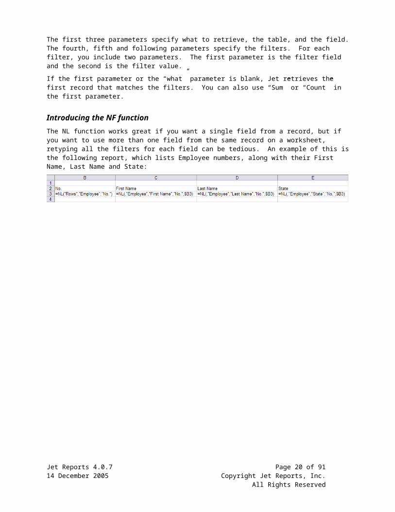
Introducing the NF functionThe NL function works great if you want a single field from a record, but if you want to use more than one field from the same record on a worksheet, retyping all the filters for each field can be tedious. An example of this is the following report, which lists Employee numbers, along with their First Name, Last Name and State:


All Rights Reserved

The employee No. uniquely identifies each employee, so we make a list of Nos., and then use it as a filter to get the names and state for each employee. A sample of the output of the report is listed below.

The NF function is a short cut that will return the value of a field in a record. One or more NF functions can be used with a single NL function with the field parameter left blank. The report listed above can be created with much less typing by using the NL and NF combined. The simpler version of the report is shown below.

As you can see, the second version requires much less typing. The output of the new report is shown below.

The new column does not contain information that you want to see on the report so we can hide this column (see Automatic Hidden Columns and Rows below).

If you drag and drop fields from the Designer with the Return “All” option selected, Jet Reports will create the appropriate NL and NF formulas for you.

Introducing Automatic Rows and RegionsThe NL function can create a copy of everything in a region of cells for each record in a group of records. The first parameter of the NL command specifies the region to copy and the filters select the group of records. When you run the report, NL expands, inserting a new copy of everything in the region, including functions and formatting, into the worksheet for each record in the group. This feature is useful for making lists of data.

To make a simple Customer phone list using the Jet Designer, you can drag the Name and Phone fields from Customer table in the Jet Designer to cells C4 and D4 respectively. Make sure that you have the Return “All” option checked at the bottom of the Designer window.

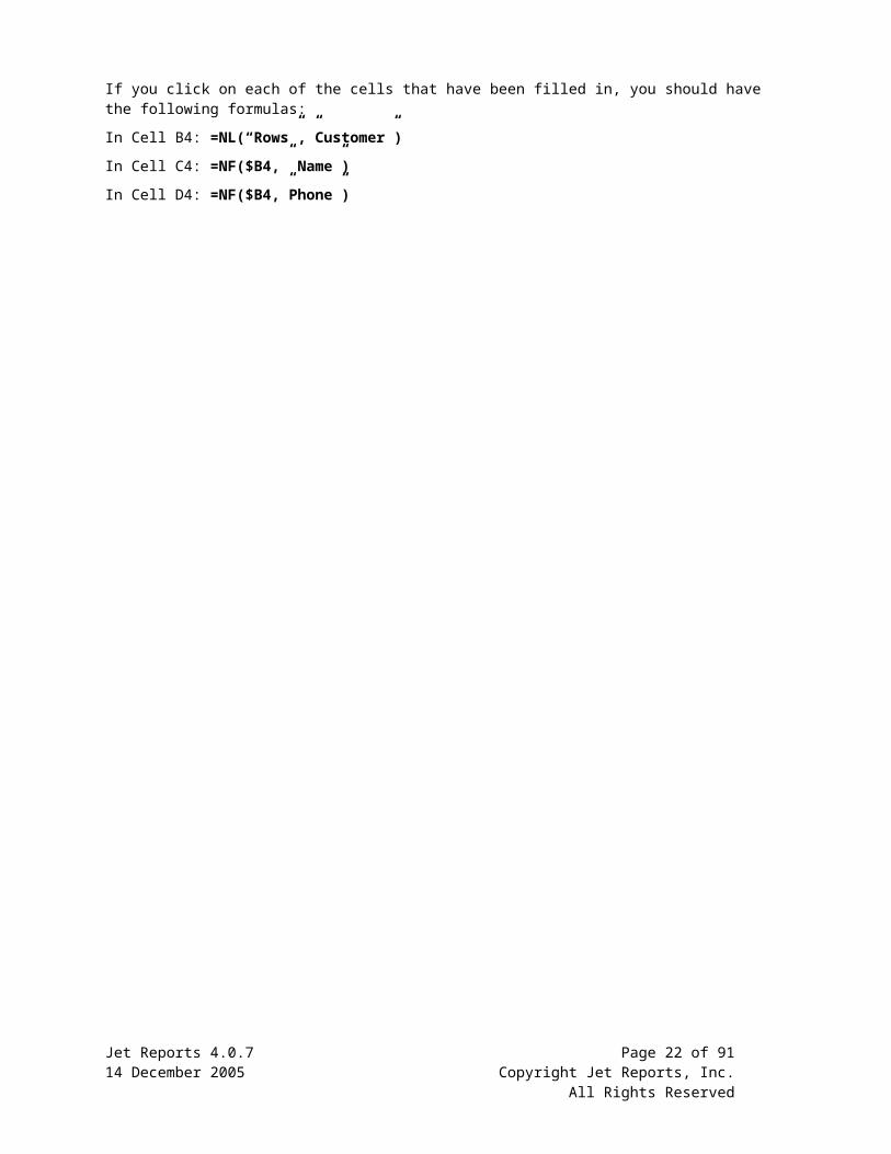
If you click on each of the cells that have been filled in, you should have the following formulas:

In Cell B4: =NL(“Rows”,”Customer”)

In Cell C4: =NF($B4,” Name”)

In Cell D4: =NF($B4,”Phone”)


All Rights Reserved

When you put Jet into report mode by choosing the menu selection Jet/Report, you will see something like the following:

When you put Jet into Report mode, the region of the NL formula is “Rows,” so Jet creates of copy of the row for each record that matches the filters. In this case, there were no filters, so Jet created a row for each customer in the Customer table. The NF functions in C and D were copied since they were inside the region, and used the record key returned by the NL function in each row. To see the NL function output in column B, you can use the Jet/Tools/Unhide menu.

You may have noticed that when you dragged and dropped the Fields into Excel, cell A1 changed to “Auto+Hide”. Jet Reports reserves Row 1 and Column A to use for marking automatically generated rows and columns, and allowing you to mark rows and columns you want to hide. Any row or column that an NL function automatically inserted will have “Auto” in column “A” or row “1” respectively. You can see the markings by using the Jet/Tools/Unhide feature as shown above. When you switch back to Design Mode, by choosing Design from the Jet menu, you will see that Jet has deleted all the rows and columns with “Auto” at the head. If you accidentally enter “Auto” in Row 1 or Column A other than in cell A1, the entire row or column will be deleted when you change from Design mode to Report mode and back.

Introducing Automatic Hidden Columns, Rows and SheetsIn the previous section, Jet Reports automatically added the key work “Hide” to the top of column B. The NF function uses the record key to retrieve fields but the record key itself does not display useful information on the report so the Jet Designer hides the record key column for you. You can use the “Hide” key word in Row 1 of any column you do not want displayed, or in column A of any row you do not want displayed. To automatically hide whole sheets, you can add the “HideSheet” key word to cell A1 of a worksheet. When you run the report Jet Reports will hide the rows, columns or sheets that you have marked with key words.

Often reports are built using calculations that are not shown on the report. Automatically hidden rows, columns and sheets provide an easy way to hide these calculations on the final report. In Design Mode, the hidden rows, columns and sheets are visible so you can make changes to the report structure.

To conditionally hide a column, put “Hide+?” in cell A2, and use a formula to return “Hide” in row 2 of the column for any column you want hidden. To conditionally hide a row, put “Hide+?” in cell B1, and use a formula to return


All Rights Reserved

“Hide” in Column B of any row that you want hidden. Formulas that conditionally hide rows or columns typically use IF functions, for example:

=IF(B4=0,”Hide”,”Show”)

Introducing Automatic Column and Row ResizingSome data values, such as customer names, are of variable length so when you load them into a worksheet cell, you do not know how wide the column should be before you run the report. If the column is not wide enough to hold the data, Excel will either display ######## in the cell, or it will only show the section of data that will fit in the cell. Jet Reports can automatically format a column or a row for the widest piece of data that you want to display. This operation is very similar to the manual sequence of selecting a column, clicking on Excel’s Format menu, then selecting Autofit Selection. The whole column will resize to fit the widest cell. If you want to resize a whole column, you can put the keyword “Fit” at the top of the column. For example if you had a list of Customer Names in column C, you would put “Fit” in cell C1 to automatically resize the column for the longest customer name. If you want to resize the height on a row, you can put “Fit” in Column A of that row.

Introducing Automatic Report ModeWhen you open a worksheet, Excel automatically recalculates all formulas, which causes all Jet Reports formulas to refresh any values obtained from Navision. However, opening a worksheet will not regenerate automatic rows or columns so if a new record was added to Navision, it will not appear in the worksheet when you open it. If you want to regenerate automatic rows and columns when the worksheet is open, you can put “Auto+Hide+Report” in cell A1 of the first worksheet in the workbook.

When you open the worksheet, Jet Reports will automatically refresh all values and regenerate all automatic rows and columns. New records added to Navision that match the filters will be included in the worksheet.

The only reason you need to use this feature is if you have automatic rows or columns created by NL functions with “Rows” or “Columns” in the first parameter.


All Rights Reserved

Introducing Report ViewersA report Viewer is an Excel user that has Jet Reports installed but is not licensed to design reports. A report Viewer is allowed to change report options and use Jet/Report but may not use any other Jet Reports features. A report Viewer may not enter Jet Functions into cell formulas or make any changes to the report design.

To design reports that a Viewer can use, you must do one of two things: lock all worksheets that contain Jet formulas, or convert the Jet Reports formulas to values.

Introducing Locked WorksheetsLocking a worksheet prevents Viewers from accidentally changing the formulas. When you select Report mode in a workbook with locked sheets, Jet saves all formulas to a hidden worksheet and does not recalculate them when the workbook opens. You create a locked worksheet by entering “Auto+Hide+Lock” in cell A1. The worksheet will be locked after the report is generated with Jet/Report and can be unlocked with Jet/Design.

If you want to create a report that Viewers can use, you should create an Options worksheet that is not locked. The Options worksheet should be used for all the reports options, such as the dates, that might change. The actual report should be on other worksheets which must have “Auto+Hide+Lock” in cell A1. You must choose Jet/Report to lock the formulas and then save the workbook.

Introducing Viewer Editable WorksheetsIf you would like to design a report that Viewers can use without locking any of the worksheets, you can instead convert the workbook to values. You do this by placing “Auto+Hide+Values” in cell A1 of any worksheet. Upon doing this, all Jet Reports formulas will be converted to values while all other Excel formulas will remain intact. The Jet Reports formulas can be restored by selecting Jet/Design. Please note that this is only applicable if you are using Excel 2003 or later.

We designed most of the sample workbooks for use by report Viewers so you can see examples of how to do this.

Sharing Reports with Excel Users Who Don’t Have Jet ReportsIn the previous two sections we introduced the +Lock and +Values keywords, which allow Jet Reports Viewers to use your reports. Both of these features are also useful for allowing people who use Excel and don’t have Jet Reports but there are several advantages to using +Values. The first advantage is that +Values does not lock the report so the person receiving the report can edit it. The second advantage is that using +Values eliminates any link to the Jet Reports add-in so Excel will not display a warning message asking the user if they want to update data from external sources. This message can be confusing to the person who receives your report. To ensure that Excel will not display the warning message, you should save the report in report mode before clicking on any Jet Reports functions. Clicking on a Jet Reports function when you have Jet Reports installed activates the drilldown button, which is a link to Jet Reports and will cause Excel to display the confusing message.

Introducing the GL FunctionReports based on the G/L are easy with the GL Formula. For example, to retrieve the balance of G/L Account 1210:

=GL(“Balance”,”1210”)

If you want to know the net change of account 1210 from 1/1/2002 thru 1/31/2002:

=GL(“Balance”,”1210”,”1/1/02”,”1/31/02”)

You can filter on three dimensions for G/L Balances. One of these dimensions is called Business Unit. The other two are Department and Project in Navision versions prior to 3.0. With Navision version 3.0 and later, the names of the dimensions can be changed, but they are generally called Global Dimension 1 and Global Dimension 2. For the balance of account “40100” with Global Dimension 1 of “USA”, Global Dim 2 of “COPPER”, and Business Unit of “US MINING” you can use the following formula:

=GL(“Balance”,”40100”,,,,”USA”,”COPPER”,,,”US MINING”)Jet Reports 4.0.7 Page 18 of 6714 December 2005 Copyright Jet Reports, Inc.

All Rights Reserved

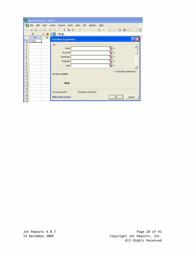
The GL Formula has many parameters so the Paste Function wizard is a convenient tool to enter the GL Function.

Introducing the Paste Function WizardJet Reports functions work with the standard Excel Function Wizard. To select a function, click on a blank cell and select menu Insert/Function or click on the Paste Function button.

The Jet Reports functions are listed under the User Defined category. Scroll to the bottom of the function category list and select User Defined. You will see the Jet Reports functions on the right.

Using Paste Function with the GL FunctionOnce you select the GL Function from the paste function wizard and click OK, you can see the available parameters for the GL Function. The window shows five parameters at a time.


All Rights Reserved


All Rights Reserved

You can scroll to see all of the parameters.


All Rights Reserved

Using Navision to Find a Table or Field Name Jet Reports adds the Jet menu to Excel but makes no modification to Navision so if you are not already familiar with the structure of Navision, you can use the Navision tools that you probably already know.

First, find the information that you want to report on in Navision, and then open Zoom from the Tools menu. Navision will display the name of the table that information is in, as well as all the fields associated with that table. The Zoom for the Customer table is below.


All Rights Reserved

Jet Reports Function Reference

The GL Function

=GL(What,Account,StartDate,EndDate,View,Dim1,Dim2,Dim3,Dim3,BusinessUnit,Budget,Company,Connection)

Purpose: Returns the budget, balance, net change, quantity, debits, or credits of a G/L Account of a given company based on filters.

Parameter Description

What Determines what the G/L functions returns: Balance, Budget, Quantity, Credits, or Debits.

Account G/L Account Number, Filter, or Range. If you specify a single totaling account, you will get totals. If you specify multiple accounts or a range of accounts, totaling accounts will not be included in the returned number.

StartDate Specify the starting date of transactions to include. If you are interested in the balance of an account on a given date, leave StartDate blank. If you are interested in the net change of an account, use Balance and specify both the StartDate and EndDate.

EndDate Specify the ending date of transactions to include.

View The G/L Analysis View to use. Leave this blank to use balances from the G/L directly. Analysis Views are available in Navision version 3 and later. This field should be blank if you are using objects from an earlier version of Navision.

Dim1 Filter for the first dimension of the analysis view. If View is blank, this is the filter for Global Dimension 1. Dimension totaling is handled the same way as Account totaling. In Navision versions before 3.0, Dim1 is used as the Department filter.

Dim2 Filter for the second dimension of the analysis view. If View is blank, this is the filter for Global Dimension 2. In versions before 3, this is the Project filter.

Dim3 Filter for the third dimension of the analysis view.

Dim4 Filter for the fourth dimension of the analysis view.

BusinessUnit Filter for the business unit.

Budget Budget filter. This is unused unless returning budgets.

Company Navision Company Name. This must be spelled the same as it appears in Navision, including case, spaces, and punctuation. If this parameter is empty (““), the company in the Jet Reports Configuration Screen is used.

Connection Connection Name as defined in Jet/Options. If this parameter is empty, the default connection is used.

ExcludeClose If you want to exclude closing dates from your GL query, enter True. If this parameter is empty, entries that were posted on the closing dates are used.

Examples:

=GL(“Balance”,”1120”)

=GL(“Quantity”,”4410”,”1/1/01”,”1/31/01”,”OCC”,”SEATTLE”)

=GL(“Budget”,”5010”,”1/1/01”,”12/31/01”,,,,,,,”2001”)


All Rights Reserved

The NL Function

=NL(What,Table,Field,FilterField1,Filter1,FilterField2,Filter2,…FilterField10,Filter10)

Purpose: Returns fields or record keys from a table based on filters and duplicates report templates.

Note: If the NL function is making copies of a template, it must be the only function in the cell. The functions =-NL(“Rows”…) and =NL(“Rows”…)*-1 are not valid functions.


What Determines what is returned.

What Description

Blank or omitted Returns the Field or record key from the first record that matches the filters.

“Sum” Returns the sum of the Field for all records that match the filters. To use Sum, the field type must be numeric.

“Count” Returns the count of all records that match the filters. Field is ignored.

“Rows” When Jet is put into Report Mode, the current row and all of its contents is copied for each unique value of Field in the records that match the filter. The values returned are sorted. To copy more than one row, put “Rows=n” where n is the number of rows to copy. For example, to copy the current row and the next two rows use “Rows=3”.

“Columns” Just like “Rows” but makes copies of columns.

“Sheets” Like “Rows” and “Columns” but the current worksheet is copied. “Sheets=n” is not supported. Only the current worksheet can be copied. The name of the sheet is set to the value returned. If the worksheet is locked, the name is limited to 22 characters. If the worksheet is not locked, the limit is 31 characters. If the values returned exceed these limits, the NL function will truncate the long names.

Positive Number 1 returns Field from the first record that matches the filter, 2 returns Field from the second record, etc.

Negative Number -1 returns Field from the last record that matches the filter, -2 returns Field from the second to last record, etc.

“Picture” Jet Reports will load a bitmap image (bmp) from a file, or from a BLOB in Navision.

“AllUnique” Returns an array of unique values of the field. If you are using Excel 2000, array size is limited. In our experience, arrays up to 5,000 elements seem to work fine. Larger arrays can cause unpredictable results. Excel 2002 or later is highly recommend if you are going to use large arrays.

“Eval” Evaluate the formula in the “Table” parameter. The formula must be enclosed in quotes and will be evaluated once when the report refreshes.

“Intersect” Returns the intersection of two arrays. See Array Calculations below.

“Difference” Returns the difference of two arrays. See Array Calculations below.

“Union” Returns the Union of two arrays. See Array Calculations below.

“DateFilter” Jet Reports will calculate a date filter using the start date and end date specified.

“Join” Join the elements of the array in the “Table” argument together into a single


All Rights Reserved

string separated by the contents of the “Field” argument.

“Split” Split the string in the “Table” argument into an array of values. The splitting is delimited by the contents of the “Field” argument.

“Filter” Returns a string value that can be used as a filter in another NL function, intended for filtering the contents of one table based on the contents of another.


Table The name or number of the table. If you want to load a picture from a file, leave the table blank.

When the “What” argument is “Rows”, “Columns”, or “Sheets”, you can use an array in the Table argument. This will cause rows, columns, or sheets to be created for each element of the array.

When the “What” argument is “Difference”, “Union” or “Intersect” this is the first array to do the calculation on.

When the “What” argument is “DateFilter”, this parameter becomes the Start Date for the filter.

Field The name or number of the field that will be returned. To return a record key, leave the Field blank. See Advanced NL Features below for Advanced Dimensions.

If you want to load a picture file, enter the full path for the file.

When the “What” argument is “Difference”, “Union” or “Intersect” this is the second array.

When the “What” argument is “DateFilter”, this parameter becomes the End Date for the filter.

FilterField1 The name of the first field by which to filter. Put “0” in a FilterField to override the default Navision Company. Put “Connection=“ in a FilterField to override the default connection. You can use multiple server database connections and a single local database connection in the same workbook.

See Advanced NL Features below for Limit=, Advanced Dimensions, and Arrays.

Filter1 The value of the filter to apply to FilterField1. If “0” is in the corresponding FilterField, put the company name here. If “Connection=“ is in the corresponding FilterField, put the connection name as defined in Jet/Options here.

FieldFieldN Same as FilterField1. Up to 10 field and filter pairs can be specified. If you specify multiple filters, they combine in a logical AND just like in Navision.

FilterN Same as Filter1.

NL Function Examples:

An NL that will return the record keys for all of the customers in the Customer table who are in the City of Boston with a Balance less than zero:

=NL(“Rows”,”Customer”,,”Balance”,”<0”,”City”,”Boston”)

An NL that returns the Customer Name from sales quote number 10000. This NL can only return one record so we left the “What” blank.

=NL(,”Sales Header”,”Name”,”No.”,”10000”,”Document Type”,”Quote”)

An NL function that returns information for a company other than the one in the Options screen:

=NL(“Rows”,”Customer”,,”0”,”CRONUS USA, Inc.”)


All Rights Reserved

An NL function that returns information for a company other than the one in the Options screen, and using a connection other than the default:

=NL(“Rows”,”Customer”,,”0”,”CRONUS USA, Inc.”,”Connection=”,2)

Create sheets called “US”,”CANADA”,”MEXICO” using an array in the table field:

=NL(“Sheets”,{“US”,”CANADA”,”MEXICO”})

Create a date filter for the month of June for 2003 if the Windows date format is set to mm/dd/yyyy – it will return “6/1/2003..6/30/2003”:

=NL(“DateFilter”,“6/1/2003”,”6/30/2003”)

This NL creates a date filter for all dates up to and including May 15, 2004 if the Windows date format is set to dd/mm/yyyy – it will return “..15/5/2004”:

=NL(“DateFilter”,,”15/5/2004”)

The NF Function

=NF(Key,Field,FlowfilterField1,Filter1,FlowfieldField2,Filter2,…,FlowFilterField9,Filter9)

Purpose: Returns a field based on a record key. Record keys can be generated with the NL function. If the field to return is a Flow Field, it is calculated based on the Flow filters.

Note: When an NL function returns a record key, Flow filters in the NL function are ignored since the record key is not a flow field. The Flow Filters from the NL function are not used to calculate the return value of the NF function.


Key Specifies the Company, Table, and Record. A Key is returned by the NL function when the Field parameter is blank.

Field Name of the field to return.

FlowfilterField1 The name of a flow filter to use in calculating the value to return. Flow filters are only used if Field is a flow field.

Filter1 The value of the filter for FlowFilterField1.

FlowfilterFieldN Same as FlowfilterField1. Up to 9 pairs of Flow filter Field and Filter pairs can be included in an NF Function.

FilterN Same as Filter1.

Examples:

=NF(A3,”Net Change”,”Date Filter”,”1/1/2002..1/31/2002”)

=NF(B3,”Name”)

=NF(B3,”City”)


All Rights Reserved

Advanced NL Function Features

Advanced DimensionsIf you have the Navision Advanced Dimensions granule, you can use a dimension code in the Field or FilterField arguments of the NL function with tables that have advanced dimensions. Jet Reports creates “virtual fields” for each of the dimension codes.

Since advanced dimensions are stored in secondary tables, this feature greatly simplifies writing reports with Advanced Dimensions. Because the data must be retrieved from two tables, using Advanced Dimensions might take longer than using fields that are in the same table.

Jet Reports will add virtual fields for dimension codes to custom tables if the custom tables are designed just like the standard tables using the same secondary tables to store advanced dimensions and the same field numbers and key structures.

Virtual fields for dimension codes will not be visible in the Designer table and field lists.

If you have created an Advanced Dimension with the same name as a field in the table from which you are pulling data, Jet Reports will use the field in the table rather than the Advanced Dimension. An example of this occurs in the Cronus database that ships with Navision. In the Sales Line table (Table 37) there is a field named Area (Field 82). In the same database, there is an Advanced Dimension named Area. If you use “Area” in an NL or NF function that references the Sales Line table, Jet Reports will use the Area Field from the Sales Line table rather than the Advanced Dimension named Area. The simplest fix for this problem is to rename the Advanced Dimension. If you do not want to rename the Advanced Dimension, you will need to pull the data out of the table that stores the Dimension Entries instead.

Array CalculationsArrays are lists of data values that you can obtain using “AllUnique” as the What parameter in an NL function. The resulting array might be a list of Customers, or a list of Invoice Document numbers, or any other list of data that match a set of filters. The array calculation operations allow you to find different combinations of two arrays. An example of when you would need an array calculation is listing the Invoice document numbers where the Type on an Invoice Line is Item for all item numbers, or a Type is G/L Account and the account number is 300. Both the Item numbers and the G/L Account numbers are stored in the same “No.” field, so there is no single set of filters that will create the list of document numbers.

The array operations available in the NL function are “Difference”, “Union” and “Intersect”. The difference between two arrays consists of all of the elements that are in the first array but are not in the second. The union of two arrays consists of a single copy of all of the elements in both arrays with any duplicates eliminated. The intersect of two arrays is the set of elements that are common to both arrays. An example of the results of the array operations are listed in the table below.

Array1: {100, 200, 300, 400, 500} Array2: {400, 500, 900, 1000, 2000}

Difference {100, 200, 300}

Union {100, 200, 300, 400, 500, 900, 1000, 2000}

Intersect {400, 500}

Example 1: This formula creates a list down rows of the union of all of the customers whose names start with A, and all the customers whose names start with B.

=NL(“Rows”, NL(“Union”, NL(“AllUnique”,”Customer”,”No.”,”Name”,”A*”),

NL(“AllUnique”,”Customer”,”No.”,”Name”,”B*”)))

Note that you could do the same operation with the following simple formula:


All Rights Reserved

=NL(“Rows”,”Customer”,”No.”,”Name”,”A*|B*”)

Example 2: This formula creates a list down rows of the document numbers of all of the invoices where the Type field is either Item, or it is G/L Account and the No. field equals 2000.

=NL(“Rows”, NL(“Union”, NL(“AllUnique”,”Sales Invoice Line”,”Document No.”,”Type”,”Item”),

NL(“AllUnique”,”Sales Invoice Line”,”Document No.”,”Type”,”G/L Account”,”No.”,2000)))

You should be cautious using arrays because they are often not the easiest, or the fastest way to solve a problem. Example 1 is a good example of a query that does not require arrays, and will run much slower if you use them.

There are two more array operations that behave a bit differently than those listed above, "Split" and "Join". "Split" will take two text strings and split the first string based on the second, resulting in an array. For instance, let's say that we would like to create a list of account numbers based on the string "1000+2000+3000". The formula would look like the following:

=NL("Split","1000+2000+3000","+")

The result would be the array {"1000","2000","3000"}.

Now, let's say we have the opposite scenario. We have an array, but would like to create a text string by joining each element of that array based on a given character. For this we would use the "Join" operation. Using the same array, we'll create a filter using the "|" character with the following formula:

=NL("Join",{"1000","2000","3000"},"|")

The result would be the text string "1000|2000|3000", which is a valid filter that we can pass into another NL function.

For each of these functions, the second argument of the NL function is the value we would like to manipulate and the third argument is the character by which we would like to join or split the value. If you experiment with these operations you will find that you have an amazing level flexibility, especially when used in conjunction with the other array calculation formulas listed above.

Filtering Based on Data from Another TableSometimes you will want to filter one table based on data that is located in a related table. Jet Reports has two mechanisms to help you do this, NL(“Filter” and “Link=”. While both mechanisms will give you the same result, which one you choose should depend on what tables you are using. NL(“Filter” should be used in situations where the primary table is larger than (or of equivalent size of) the secondary table (i.e. the Sales Line table filtered off of the Sales Header). “Link=”, on the other hand, will greatly increase performance when the primary table is smaller than the secondary table (i.e. the Dimension table filtered off the G/L Entry). Please see the sections below for examples.

When performing cross-table filtering you may not be able to drilldown on the cell. That is because Navision will not accept a list as a filter, so Jet Reports attempts to create a set of filters that will uniquely select the exact same records. This is often possible when there are only a few records selected. However, if there are too many records, Jet Reports will report that drilldown is not possible.

Using NL(“Filter”)As stated above, NL(“Filter” should be used when you would like to filter one table based on data from another table that is smaller or of equivalent size (if this is not the case, please see the section below on “Link=”). For example, the Sales Line table is generally larger than the Sales Header since each Document can have several lines associated with it. The Sales Line table does not have the Posting Date in it, but the Sales Header does. The Document Number is common to both tables, so if you wanted to list Sales Lines based on a Posting Date, you would start out with an NL formula like the following:

=NL(“Rows”,”Sales Line”, ,“Document No.”,{List of Document Nos. with Posting Dates 1/1/02..1/31/02})


All Rights Reserved

We need to replace the English description of the list in the formula above with an NL formula. The field in the Sales Header that holds the document number is “No.”, so the NL formula that generates a document number filter is below:

NL(“Filter”, ”Sales Header”, ”No.”, ”Posting Date”, ”1/1/02..1/31/02”)

Finally, we need to replace the English description in the first formula with the second formula as shown below:

=NL(“Rows”,”Sales Line”, ,“Document No.”,NL(“Filter”,”Sales Header”,”No.”,”Posting Date”, ”1/1/02..1/31/02”))

There is one NL function inside another. The inner NL function returns the Document No. filter that is then used in the Sale Line table.

Using “Link=”As stated above, “Link=” is another mechanism that can be used to filter data in one table based on data in a related table. Specifically, “Link=” should be used when the primary table is smaller than the secondary table. For example, let us say you would like to create a list of invoice numbers that contain item sales. You can list the invoice numbers from the Sales Invoice Header table, but will need to use the Sales Invoice Line table to ensure that each invoice contains an item sale. Since all you would like to do is create a list of invoice numbers, you do not need a complete list of Sales Lines for each invoice. Rather, all you want to know is whether an entry containing an item sale exists. To do this, your formula would look something like the following:

=NL(“Rows”,”Sales Invoice Header”,”No.”,“Posting Date”,”7/1/05..7/31/05”,”Link=”,”Sales Invoice Line”,”Document No.”,“=No.”,”Type”,”Item”)

Note that the first argument after the “Link=” is the name of the secondary table. The successive arguments thereafter represent FilterField/Filter pairs that will be applied to this table (i.e. “Document No.” and “Type” are fields in the Sales Invoice Line table, not the Sales Invoice Header). Filter values with an equals sign (‘=’) pre-pended to them represent the linking fields from the primary table. In the above example, the NL function will examine the value of the No. field for each record in the Sales Invoice Header table and will only include the record if a corresponding record exists in the Sales Invoice Line table where the “Type” field is “Item” and the “Document No.” field is equivalent. Note that there can be multiple linking fields.

Blank FiltersSometimes you want to filter an NL function based on the output of another NL function which could return a blank value. The NL function does not allow you to use blank filters, and you will get a #Value error message if you fill in a FilterField parameter and leave the corresponding Filter blank. A good example of this would be in the case of retrieving an Item Description based on the output of an NL that listed Item Nos from Sales Invoices. You could have Sales Invoices that do not have item numbers so the NL command would return a blank value. This is where you need to use Excel’s IF function. Assume that an NL function that lists item numbers is in cell C4. If cell C4 is blank, we want cell D4 to be blank too. Otherwise, we want to filter an NL in D4 based on the contents of C4.

The first step is to test cell C4 to see if it is blank. Excel will do that for you using the following formula:

C4=””

The formula above uses two double quote characters to represent a blank cell and gives you a True/False response.

The NL function to retrieve the Item Description looks like this:

NL (1,”Item”,”Description”,”No.”,C4)

Combining the two functions above into an IF function looks like this:

=IF(C4=””,””,NL (1,”Item”,”Description”,”No.”,C4) )


All Rights Reserved

The spreadsheet below has the results of each of the formulas described above:

The example above assumes that blank values are not something you would want to find. Sometimes you want to find all records that have a blank value. If you simply want to find all of the blanks, then you can use the Navision filter for blank, which is two single quotes (‘’). In the above example, if C4 could be blank and we want to use it as a filter anyway, we can use the following formula:

=NL (1,”Item”,”Description”,”No.”,”’”&C4&”’”)

Although this formula is a little hard to read, it is putting a single quote character (‘) on either side of the C4 reference. The & function is an Excel function that combines two bits of text into one so the result of this formula will be adding a single quote character on either side of the value in cell C4. If C4 contains the Item No. of Shampoo1, the resulting filter will be ‘Shampoo1’. If C4 is blank, the result is ‘’ (two single quotes), which is a valid Navision filter for blank.

An easier to read variation on the filter for blanks above is to put “@@” in front of the value in C4. The function becomes:

=NL (1,”Item”,”Description”,”No.”,”@@”&C4)

Please refer to the “Filtering a Query” and “Special Characters in a Filter” sections below for more information.

Calculating Date FiltersThere are many times when you want to make your report very easy for the end user to work with, but need to use variable date ranges to retrieve the data for the report. An example of this would be a report that can list the sales activity for the month, the year to date and the previous year for the sake of comparison. Instead of requiring the user to enter all of the date filters that the report needs, you can calculate the date ranges based on a single start date. The formulas for calculating various dates relative to a start date are detailed below in the Excel section.

Assuming that D4 contains the first of the month, the formula for calculating the filter for the whole month is listed below:

=NL (“DateFilter”,D4, Date(Year(D4), MONTH(D4)+1, 1)-1)

If D4 equaled 2/1/2003, the result of the formula would be 2/1/2003..2/28/2003

The formula for calculating the filter for the year to date for the month in cell D4 is listed below:

=NL (“DateFilter”, Date(Year(D4), 1, 1), Date(Year(D4), MONTH(D4)+1, 1)-1)

If D4 equaled 2/1/2000, the result of the formula would be 1/1/2000..2/29/2000. Note that Excel will take care of leap years for you.

The formula for calculating the filter for the same month last year for the month in cell D4 is listed below:

=NL (“DateFilter”, Date(Year(D4)-1, Month(D4), 1), Date(Year(D4)-1, MONTH(D4)+1, 1)-1)

If D4 equaled 5/1/2004, the result of the formula would be 5/1/2004..5/31/2004.


All Rights Reserved

Evaluating FormulasThere are some cases where you will want to evaluate a formula only once for each time you run your report. A good example of this is the Now() function. You generally want the Now() function to run once when you update the report, and otherwise remain inert. You can use the NL formula to control when a formula updates by putting “Eval” in the What parameter. The formula you want to evaluate goes in the “Table” parameter of the NL function and it must be in quotes. If you are evaluating a formula that already has quotes inside the formula, then Excel requires you to use two sets of quotes instead of one. Some examples are listed below.

This function will calculate Now once each time the report updates:

=NL(“Eval”,”=Now()”)

If you wanted to calculate a date filter for the current month, you could start with this formula:

=NL(“Datefilter”,Date(Year(Now()),Month(Now()),1),Date(Year(Now()),Month(Now())+1,1)-1)

The formula above uses the Today function liberally, so you should put it inside an NL(“Eval”…) formula, and change “Datefilter” to “”Datefilter”” with two sets of quotes:

=NL(“Eval”,“=NL(“”Datefilter””,Date(Year(Now()),Month(Now()),1),Date(Year(Now()),Month(Now())+1,1)-1)”)

Note that you must place any volatile Excel function (i.e. NOW() and TODAY()) directly inside the NL(“Eval”) to avoid constant recalculation, even if the volatile function has no other dependant cells. A cell reference is not sufficient. For instance:

=NL(“Eval”,”=NOW()”)

will only be calculated once with each run of the report, whereas,

=NL(“Eval”,”=B4”), where B4 contains a volatile function, will be constantly recalculated. This will result in a major performance hit and should be avoided.

Faster Reports Using Formula Evaluation Another extremely useful application of the NL(“Eval” …) function will improve your report execution time if you have an Options page and you have cell references to filters on the Options page. When your report runs, Excel tries to recalculate any formula on each page where the cell references have changed. Unfortunately, when you have cell references that extend outside the page where the formula is located, Excel does not know when that external reference may have changed so it will recalculate the formula any time the current worksheet changes. As you may have noticed, Jet Reports changes worksheets many times over the course of evaluating a report so Excel reacts by forcing recalculation of any formula that has off-sheet cell references. You can eliminate this unnecessary recalcuation by using the NL(“Eval”…) function to bring the values from any off-sheet reference onto the local worksheet, then change your cell references to only use the local cell where you have the NL(“Eval”…) function. For example, if you had a Profit and Loss report, you would probably have a changeable Start Date and End Date on the Options page with cell references on a Detail page and a Summary page. Instead of having many cell references to the Start Date and End Date, you can name the cells StartDate and EndDate respectively (see Useful Excel Features section for information on Named Ranges), and use the following two formulas to bring the data in the two cells onto the Detail and Summary page:

=NL(“Eval”,”=StartDate”)

=NL(“Eval”,”=EndDate”)

If you put these two formulas in cells B2 and B3 respectively, you can then use local cell references for your filters, eliminating a large amount of Excel calculation overhead.

Evaluating Excel formulasThe NL(“Eval”) function will evaluate any Excel function including cell references. Simply enter “Eval” as the “What” of your NL function and your desired Excel formula, including the “=” sign, as the “Table” argument. (Be sure to put quotation marks around your formula.) Your formula should look something like this: =NL(“Eval”,”=C5”). This will display the value in cell C5.


All Rights Reserved

Sometimes you need to reference cells on other worksheets inside of your workbook. Usually, this occurs when you have provided an “Options” sheet for your users which many of your Jet Reports formulas reference. This gives users the ability to update reports based on new filter criteria. You can accomplish this by using the same formula as before only including the worksheet name followed by an “!” as part of your cell reference. =NL(“Eval”,”=Options!C5”) will display the value from C5 of the worksheet named “Options”.

In Jet Reports versions prior to 3.7.2 you will need to add the Workbook name as part of the cell reference to prevent Excel from displaying the “Update Values” window (pictured below) when calculating your NL(“Eval”,”=Options!C5”) formula. When you include the Workbook name as part of your cell reference you need to put the Workbook name in brackets “[]”. The resulting formula should look like: =NL(“Eval”,”=[Book1]Options!C5”) and will give you the value from C5 on the “Options” worksheet from “Book1”. In Jet Reports version 3.7.2 and later you do not need to include the Workbook name as part of your cell reference.

If the cell you are trying to reference is on a worksheet that has a space in its name you will need to wrap the worksheet name in apostrophes as in the following formula:

=NL(“Eval”,”=’Options Page’!C5)

To add the workbook name to the cell reference you will need to place the workbook name inside of the apostrophes as well as in the follow formula:

=NL(“Eval”,”=’[Book1]Options Page’!C5”)

Named ranges with NL(“Eval”)NL(“Eval”) can be used with named ranges as well as cell references. So, assuming you named cell C5 on your “Options” worksheet “DateFilter” you can use the cell’s name as if it were a normal cell reference. =NL(“Eval”,”=DateFilter”) will give you the value of cell C5 on your “Options” worksheet. You do not want to include the Worksheet name or the Workbook name with the named range.

Jet Report formulas that reference another worksheetOnce you have the NL(“Eval”) formula working correctly you can then have the rest of your Jet Reports formulas reference the cell with this formula instead of your “Options” worksheet. If you have multiple filters on your “Options” worksheet you write one NL(“Eval”) formula for each filter. Then have your Jet Reports formulas reference the relevant NL(“Eval”) formula.


All Rights Reserved

Example:

If your NL(“Eval”) formula is in cell E3 then your Jet Reports formulas would look like this: =NL(“Rows”,”Customer”,”Name”,”City”,E3). See Fig. 2 through 4 on the following pages.

Fig 2 “Options” worksheet

Fig. 3 NL(“Eval”) that references the “Options” worksheet. Workbook name included.


All Rights Reserved

Fig. 4 Jet Reports formula with reference to the NL(“Eval”) formula.

Using NL(“Sheets”) with NL(“Eval”)There is one exception to the information presented above regarding NL(“Eval”). If you have an NL(“Sheets”) function on the same worksheet as NL(“Eval”), you cannot use cell references on another worksheet directly in the NL(“Eval”) function. You need to first use a cell reference in an another cell to copy the value you are interested in to the current sheet, then use NL(“Eval”) to evaluate the local cell reference. For example, if you have a Profit and Loss report that is creating a worksheet per department, you probably also have a Posting Date filter that you use in each department sheet. If the posting date filter is in a cell named DateRange, you could put the following formula in cell C3 of the department worksheet:

=DateRange

You could then put the following formula in cell D5:

=NL(“Eval”,”C5”)

All of the functions that need to use the date filter can use cell D5 on the report page to access the DateRange cell.

Excluding Closing DatesYou can exclude posting dates from your query when you are using date filters by putting <>C& in front of your date filter and you will no longer include the closing date. The example below is using the Cronus US database, which has a closing date of C12/31/99.

=NL(“Sum”,”G/L Entry”,”Amount”,”Posting Date”,”<>C&12/31/99..1/1/01”,”G/L Account No.”,54701)

Filtering a QueryWhen you enter criteria, you can use all the numbers and letters that you can normally use in the field. In addition, you can use some special symbols or mathematical expressions. Here are the available formats:

Meaning Sample Expression Records Displayed


All Rights Reserved

Equal to 377

BLUE

Number 377

Those with the BLUE code, for example, the BLUE warehouse code

Interval 1100..2100

..2500

..12/31/2000

8..

Numbers 1100 through 2100

Up to and including 2500

Dates up to and including 12/31/2000

Everything after 8.

Either/or 1200|1300 Those with number 1200 OR 1300

And <2000&>1000 Numbers that are less than 2000 AND greater than 1000.

The & sign must be used with a range because no single record can have two values. An example of an invalid use of & is A&B because no records can be equal to A AND equal to B. An example of a valid use of & is A*&*B, which means find all records that start with A AND end with B.

Different from <>0 All numbers except 0

Greater than >1200 Numbers greater than 1200

Greater than or equal to >=1200 Numbers greater than or equal to 1200

Less than <1200 Numbers less than 1200

Less than or equal to <=1200 Numbers less than or equal to 1200

An indefinite number of unknown characters

*Co*

*Co

Co*

Text that contains "Co"

Text that ends with "Co"

Text that begins with "Co"

See “Wildcard Filters” section below.

One unknown character Hans?n Text such as Hansen or Hanson

See “Wildcard Filters” section below.

Calculate first 30|(>=10&<=20) Number 30 OR with a number from 10 through 20 (the result of the calculation within the parentheses)

Ignore special characters

Special Character List:

@@A&B Those equal to “A&B” – the & is a part of the value instead of being interpreted as an AND operator.


All Rights Reserved

&, @, |, (, ), =, ?, >, <

Two periods in a filter also constitute a special character

‘A&B’|’M&M’ Those equal to “A&B” OR those equal to “M&M”. The | is interpreted as a logical operator as described above.

If you need to combine two filters that both have special characters, you can enclose your filters in single quotes.

Check Special Characters in a Filter section below for examples.

“@@”&C3

Or

“’”&C3&”’”

Or

“’”&C3&”’|’” &C4&”’

Where C3 and C4 could contain blank or special characters like the following:

John(Huston)

Ben & Jerrys

Use “@@” & <Cell Reference> if the cell reference could be blank and you want to filter for blank field values.

Use the ‘ character in double quotes added before and after a cell reference to always have a safe filter from the cell reference.

The two methods listed above are equivalent for a single filter. If you want to combine two cells with filters in them, you must use ‘ as in the bottom example.

Ignore case (either uppercase or lowercase allowed)

@location Text such as LOCATION, location or LocatioN

You can also combine the various filter expressions (See Also “Wildcard Filters” below):

5999|8100..8490 Include any records with the number 5999 OR a number from the interval 8100 through 8490.

..1299|1400.. Include records with a number less than or equal to 1299 OR a number equal to 1400 or greater (all numbers except 1300 through 1399).

>50&<100 Include records with numbers that are greater than 50 AND less than 100 (numbers 51 through 99).

*C*&*D* Text containing both C AND D.

@*co?* Text containing co, CO, Co, cO, such as cot, cope and incorporated.

CO, cO, Co or co must be present, followed by at least one character, but there can be an indefinite number of characters before and after these, and case is unimportant.

Note:

It is important that you enter only meaningful filters. For example, it is possible to specify a posting date range that does not have any records in it, and Jet Reports cannot check this for you.


All Rights Reserved

Limiting the Number of Records in a QueryYou can place a limit on the number of records that NL will return by entering “Limit=“ in one of the FilterField parameters and entering a maximum number in the corresponding Filter parameter.

The following example will print the Customers with the ten largest sales.

=NL(“Rows”,”Customer”,”Name”,”-Sales ($)”,”*”,”Limit=”,10)

Loading PicturesTo load a bitmap from a file, leave the table blank, and put the file name in the Field parameter. To use a picture that is stored as a BLOB in Navision, enter the Table, Field and Filter parameters that will select the correct BLOB. You can enter “Height=” and “Width=” in the FilterFields to set the height and width of the picture and, in the corresponding Filter, you can enter the height and width number. If you do not enter sizing specifications, Excel will choose a default size for the picture.

An NL function that will display a picture from the database for Item 10000:

=NL(“Picture”,”Item”,”Picture”,”No.”,10000)

An NL function that will display a picture from a file with the height and width specified:

=NL(“Picture”,,”C:\testdb\picture.bmp”,”Height=”,25,Width=”30”)

Look at the Inventory with Pictures sample report for an example of this.

Grouping Data ListsSince you can create a dynamic list using an NL function, the next logical step is to group the items in the list. The mechanism for grouping is nesting NL functions. When one NL is inside the region of another, the NL functions are nested. The outer NL function lists the grouping criteria, and then the inner NL can use the results of the outer NL as a filter. When you select report mode, the outer NL will evaluate first, inserting copies of its region for each record and filling in its data values. Once the outer NL has expanded, the inner NL will expand, making copies of its own region. Jet Reports evaluates the NL functions from left to right, and top to bottom so if you have put one NL function that acts on rows in cell D4, and one that acts on columns in cell B5, Jet Reports will evaluate cell B5 first.

Grouping Data ExampleA simple example of a grouped list is listing Customers who have sales along with their sales grouped by state and subtotaled. Since we are listing Customers, one good place to start is the Customer table. We want to first list customers who have sales, then we can worry about the grouping later. The Sales ($) flow field works well as a filter field for our purpose. If we drag and drop the Name, State and Sales ($) field out of the Designer, then edit the resulting NL to filter for Sales ($) <> 0, we will end up with something resembling the picture below.

If we run the report we will get a complete list of customers, who have sales. The next step is to group the customers by State. The overall idea is that we want to list unique states that have customers with sales, then use that list as a series of filters for the existing NL that lists customers. To achieve this goal, select Unique in the designer, then drag and drop the state field into the cell that is one row up and one column to the left of the existing Jet Reports 4.0.7 Page 37 of 6714 December 2005 Copyright Jet Reports, Inc.

All Rights Reserved

NL command. In the picture above, the cell you should be dropping into is cell C3. Next we can add the same filter field, filter pair as the previous NL command for Sales ($) <> 0. If we run the report, we will get a list of state names, then a list of customers as shown below.

Note that the column headers of Name, State and Sales ($) all got copied in the region of the NL command. Also note that the first customer State is blank. In this case, the customers outside the US have a blank state so it is a valid value that we should preserve.


All Rights Reserved

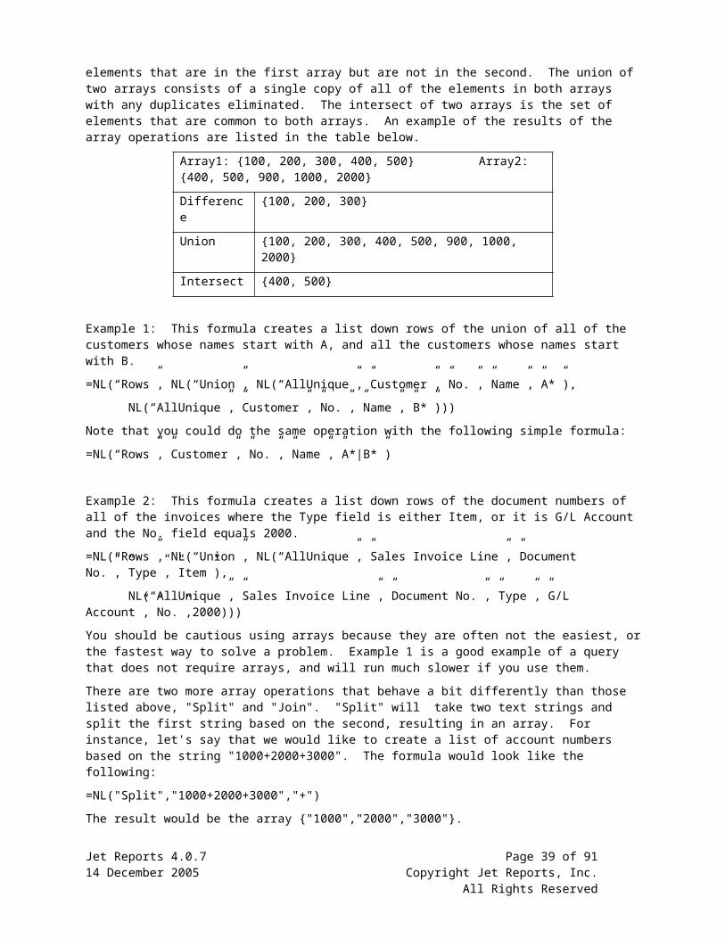
The next step is to change the NL command listing States in C3 from “Rows” to “Rows=2”, which will nest the two NL commands as described above. Now when the report runs, Jet Reports will copy rows 3 and 4 for each state, including the customer list. Finally, we can add a filter to the NL listing customers to filter by the state cell. Since we could have blank states, we need to pre-pend “@@” to the beginning of the filter so the formula will look like the picture below.

If we run the report, we will get a list of states, then a list of customers under each state. The final task is to add a subtotal by state for the Sales ($) field. This can be a simple Sum function if you don’t want a grand total, or a Subtotal function if you do want a grand total. For the sake of the complete example, we will calculate subtotals and a grand total. The first Subtotal function goes one row below the NL listing Customers. For a complete explanation on the relative location of the subtotal function, refer to Useful Excel Features below. The function should look like the one pictured below.

Note that both rows 4 and 5 are included in the range of the Subtotal function. Next, we need to expand the Rows=2 of the NL that lists States to include rows 3-6 so our new subtotal command will fall into the region that gets copied. For asthetics, we can include row 7 so we have a blank line between states. The “Rows=2” becomes “Rows=5”. Now we need to add our Grand Total. Since we have 5 rows in the region on the State replicator, we need to skip row 8 and put our grand total on row 9 as shown below.

Finally, we can run the report and get a complete list of customers who have sales, grouped and subtotaled by state.


All Rights Reserved

Multi-level GroupingIt is often the case that we want our report to contain more than one level of grouping. For instance, let’s say we want to add more detail to the above example by not only grouping the customers by state but by city as well. The result would be a list of customers grouped by city, grouped by state. The first thing we need to do is to create room for this intermediate level of grouping by inserting a column between C and D, and a row between 3 and 4. We can also move our column headings down to the newly inserted row 4, as shown in the picture below.

The next thing we need to do is add the formula to insert our list of cities. Open the Customer table in the Jet Designer, select the Unique return option, and drag the City field into cell D4. Note the stair-step pattern of the three NL functions, which is the standard format for grouped reports. Just as we did in the previous example, we must link our list (cities, in this case) to the grouping criteria (the state) using a filter, as shown below.

Just as we did before, we will we have to adjust the size of the replicator regions to account for the new level of grouping (in effect, nesting the NL functions). In order to do this, we have to change the What argument in the newly added NL function from “Rows” to “Rows=2” and in the NL function listing states from “Rows=5” to “Rows=6”. We do not need to adjust the subtotal (we will still do a subtotal by state) by since we have increased the size of the outermost region we will have to move our grand total down one row. This will allow for the anchor row, as shown in the picture below.


All Rights Reserved

If we run the report as is we see that the first city under each state is the only one for which the customer list does not return an error. In order to see the source of the error we select Jet/Tools/Unhide, select cell E9, and press the F2 key. This highlights the cell references that the formula is making and indicates to us that we’re attempting to use a blank filter (selecting Jet/Debug will give us an error message that confirms this). This is a standard problem when doing a multi-level grouping. What we need to do to resolve it is to copy the value from cell C3 over into column B and down, filling the 6-row region of our replicator, as shown below.

Note that we do not want to copy and paste the formula from cell C3, but rather set each cell equal to the adjacent cell (in cell B3 we have “=C3”, in cell B4 we have “=B3”, etc.). Next, we need to adjust the filter in cell E5 to refer to the value (state) that is on the same row to ensure we do not lose the cell reference. Finally, we add a filter to the NL formula in E5 to group the customer lists by not only the state but the newly inserted city as well. See the example below.

If we run the report seen above we will obtain a list of customers grouped by state, grouped by city as stated in the goal. Note that we can add as many levels of grouping as deemed necessary (for instance, we could further expand this example by adding order details by customer).

SortingNormally, sorting is in ascending order based on the Field values returned; however, you can override the normal sorting and sort in ascending order or descending order based on any field in the table you are using. If you want to sort ascending, put a “+” followed by the field name in the FilterField parameters. To sort descending, put a “-” followed by the field name in the FilterField parameters. The filtering properties of the FilterField remain intact so you can enter a filter in the Filter parameter. If you want to sort on a field without a filter, put a “*” in the corresponding filter since blank filters are not allowed.

Examples of sorting using FilterFields:

An NL function that sorts by Search Name while filtering for Search Name starting with B:

=NL(“Rows”,”Customer”,,”+Search Name”,”B*”,”Sales ($)”,”<>0”)

An NL function that sorts Customer Names by state (in ascending order) then by the sales (in descending order) in each state:

=NL(“Rows”,”Customer”,”Name”,”+State”,”*”,”-Sales ($)”,”<>0”)


All Rights Reserved

Using Navision Keys to Optimize SortingJet Reports can sort on any Field but if you are sorting in ascending order, you can easily improve the performance of the report by adding a Navision Key to the table that you are searching. To maximize performance, the key should have all of the fields you are sorting on, in the same order as they appear in your NL function. If you do not know how to add a key in Navision, contact your Navision Solutions Center for assistance. If you are returning a field with the NL command, this field also needs to be included in the key to optimize speed.

Jet Reports Sorting vs. Navision SortingBy default, Jet Reports will allow Navision to perform all sorting. This is generally preferred because Navision uses keys to sort and is very fast as a result. If a key that matches the filters exactly is not found, however, Jet Reports will sort the resulting data list internally. The following examples illustrate the fields needed in a key to guarantee that a Code field is sorted the same as Navision:

An NL that sorts by state, then by Customer No.

=NL(“Rows”,”Customer”,”:No.”,”+State”,”*”,”Sales ($)”,”<>0”)

The key that will sort correctly needs to start as follows:

State, No.,…

This can be followed by other fields. Since No. is the primary key, it is included automatically at the end of the key so the key of State would suffice.

In some situations, allowing Jet Reports to perform the sort may result in a sort order that seems inconsistent, especially in the case of Code fields. Code fields (i.e. “No.” in the “Customer” table) can contain both numbers and letters, and they sort differently depending on whether you are using a native Navision Server or a Navision SQL Server (please see the Navision Help C/Side Reference Guide for details). Jet Reports’ internal sorting mechanism, on the other hand, will sort everything textually, i.e. “10” < “100” < “20”. Items in a textual sort are compared on a character-by-character basis. If you would like to force a textual sort but are using filters that match a key in Navision, you can do so by simply switching the order of two of the filters or adding an extraneous filter at the end of the formula

Special Characters in a FilterCharacters such as |><=.()&@ are considered special characters by Jet Reports. If you need to include any of these characters as part of filter value then you need to precede the filter with “@@”. The “@@” will pass the filter in as a literal string and be evaluated properly. If you have two periods (.) in a filter string, i.e. “A.M.” the filter includes special characters.

Example:

If you need to filter by a Customer named “John(Houston)” you will need to place the “@@” in front of “John(Houston)”. The resulting formula would look like this:

=NL(“Rows”,”Sales Invoice”,”No.”,”Customer”,”@@John(Houston)”)

Since the name John(Huston) would often be located in an adjacent cell, this is the equivalent formula using a cell reference instead:

=NL(“Rows”,”Sales Invoice”,”No.”,”Customer”,”@@”&C3)

If you need to combine several filters together that all include special characters you need to enclose each filter item in single quote characters (‘) instead.

Example:

If you need to filter by Customers named “John A.M.” or “Ben & Jerry’s”, you will need to use the verticle bar (|) to be a logical OR. If there were no special characters, your filter would look like the following:

=NL(“Rows”,”Customer”,”Name”,”Name”,”John|Ben”)


All Rights Reserved

Since we have two names that both contain special characters, we cannot use the @@ since we still need the | to evaluate as a logical OR, instead of a special character. The following formula shows the proper (if a bit hard to read) method of constructing the filter:

=NL(“Rows”,”Sales Invoice”,”No.”,”Customer”,”’John A.M’|’Ben & Jerry’s’”)

Again, these names could be coming from cell references, so the equivalent formula with cell references is beow:

=NL(“Rows”,”Sales Invoice”,”No.”,”Customer”,”’”&C3&”’|’”&C4&”’”)

Check the table in “Filter a Query” above for more syntax examples.

Wild Card FiltersThe * and ? are wild card filters. Wild card filters cannot be used as part of a range filter when you are trying to exclude the elements of the range. This means that filters, such as: <>A*..C* are not allowed. Likewise, <>A?..B? is not a valid filter. If you want to create a filter that will exclude everything starting with A through C, you need to think of the filter as including everything except the things starting with A through C. When you think of the filter as including values, then D.. is the filter you would use. Note that for this example, <>A*&<>B*&<>C* would also work since there are no ranges involved.

Advanced Jet Reports Features

Aborting a Long CalculationIf a worksheet calculation takes longer than two seconds, Jet Reports will display a status window with calculation information in it. If you want to abort the current calculation, you can click the Cancel button. If Excel is in the middle of a calculation, the cancel button can be slow to respond, but when Excel is finished with the calculation, the report will stop refreshing and the uncalculated cells will display #VALUE.

Building a Report from Multiple DatabasesIf you want to build a report that uses multiple databases of any type, you need to create a connection for each database. Check the installation manual to find information on configuring connections. Once you have your connections configured, you can specify separate connections in both the NL and the GL function. You can change the connection that the NL command uses by specifying “Connection=” as a Filter Field and the connection name as a Filter. The Jet Designer will do this automatically if you are dragging and dropping from a connection that is not the default connection. The GL command has a separate parameter that will accept the connection name. You can find more information on the syntax of these commands in the Reference section above. An example of a report summing the amounts from Purchase Invoice number 1000 from a Navision database and a Northwind Access database might use the following formula:

=NL(1,”Purch. Inv. Header”, “Amount”, ”No.”, ”1000”, ”Connection=”, ”Navision370”)

+NL(1,”Orders”,”Amount”,”OrderID”,”1000”,”Connection=”,”NorthWind”)

In this example, we have a connection named Navision370 that connects to a Navision database and a connection named NorthWind that connects to the NorthWind Access database. An important point to notice is that if you and a colleague were both going to use the same report, you would need to have your connections named the same.

Codes & Nos. with Special CharactersCharacters used in Navision filters like “&”,”|”, and “..” should not be used in Codes or Nos. In addition, you should not use blank Codes or Nos. Using blanks and these characters in your Navision data will cause problem with reporting and filtering in both Navision and Jet Reports. Fortunately, it is rare to find blank Codes and Nos. or to use special characters in Codes and Nos.


All Rights Reserved

When Field Values contain filter characters like “&,” you must put the field values in single quotes to use them in a filter. For example, if customer IDs have embedded “&” you can filter on the customer ID as follows:

B2=NL(“Rows”,”Customer”,”No.”)B3=NL(,”Customer”,”Name”,”No.”,”'“&B2&”'“)

Note the customer number is in a formula that surrounds it with single quotes: “'“&B2&”'“. This causes Navision to consider any embedded special characters as part of the field value and not as special characters.

Conditionally Hiding a Column, Row, or SheetTo conditionally hide a row, put “Hide+?” in cell B1, and use a formula to return “Hide” in Column B of any row that you want hidden. You can conditionally hide a column by entering “Hide+?” in cell A2, and using a formula to return “Hide” in row 2 of the columns you want hidden. Similarly, with “Hide+?” in cell A2 you can place a formula in cell B2 that conditionally returns “HideSheet” in order to hide the entire worksheet. Formulas that conditionally hide rows, columns, or sheets are typically IF formulas, for example:

=IF(C4=0,”Hide”,”Show”)

Debug and Local Database ConnectionsIf you attempt to use more than one local database connection in a workbook, you will see #VALUE for the results of one of them. When you use Jet/Debug, the function may calculate correctly. This is because when you run Debug, Jet closes all other local database connections to analyze the cell you have selected. The #VALUE occurs because each workbook can only have a single local database connection open at a time, so you can only include data from a single local database in a workbook. You can include data from multiple server database connections on the same workbook with no problems.

Design Mode CalculationsSome functions return different values in design mode than in report mode. In design mode, the first record that matches the filter is returned. In report mode, if a function requires a sort, the first record based on the sort is returned. This makes design mode calculations faster while still generating accurate reports.

DrilldownWhenever you make a change to the worksheet, the drilldown button is turned off. This is because displaying the drilldown button removes the ability to undo changes. To perform a drilldown when the drilldown button is not displayed, use the menu option Jet/Tools/Drilldown. After choosing Jet/Tools/Drilldown from the menu, the drilldown button will remain enabled until the next change is made to the worksheet.

You can put multiple NL, GL, or NF functions in a cell, but only one is used for the drilldown. If there are multiple functions in one cell, the function that Jet Reports will use for drilldown is unpredictable, so if you want a predictable drilldown, put only one NL, GL, or NF function in each cell.

The value reached by the drilldown could be different from the value displayed in the cell if the database has changed since you last refreshed the workbook.

Drilling down from a formula with an NL function that contains “Rows”,”Columns” or “Sheets” in the first argument may not return the expected result. These formulas return multiple values and the drilldown result is unpredictable. Usually, these formulas are in hidden rows or columns so this is generally not a problem.

If you use Array Filters, you may not be able to drilldown on the cell. That is because Navision will not accept an array as a filter, so Jet Reports attempts to create a set of filters that will uniquely select exactly the same records as the array filters. This is often possible when there are only a few records selected. But if there are too many records, Jet Reports will report that drilldown is not possible.

The drilldown form displayed in Navision depends on the table in the function. Some tables contain values that are derived from other tables. For example, the Sales ($) field in the Customer table is derived from the Cust. Ledger


All Rights Reserved

Entry table. If you want a drilldown that shows the records in the Ledger table, you need to use a sum formula on that table instead of using Sales ($) from the Customer table.

If Navision is already open but you have minimized its window, you must manually switch the Navision window to see the drilldown results. If the window is not minimized, Navision will automatically become the foreground application.

Improving Report PerformanceIn order to speed up the run-time of your reports, do your best to follow these guidelines:

Apply filters in Jet Reports that will match a key that is already in your Navision Database. Also, if you are applying sorts in your formulas, make sure the order of the sort fields are in the same order as a Navision key. (also see “Sorting”,)

Whenever possible, use NL functions to retrieve record keys rather than unique values, then use the NF function to obtain field values from them. An NF function does not have to make a request to the database, while an NL function does. (also see “Jet Reports Function Reference”)

When you would like to retrieve a single piece of data that is in a row or column that already contains a replicator, use a Data Retrieval NL function with a “1” as the “What” parameter. (also see “The NL Function”)

When filtering across tables, be sure to choose either NL(“Filter”) or “Link=” appropriately. (also see “Filtering Based On Data from Another Table”)

Avoid bringing large amounts of data into the spreadsheet and using conditional hide to eliminate the data you do not want to see. In many cases, using an appropriate filter from another table will eliminate the data you do not want to see. (also see “Filtering Based On Data from Another Table”)

Avoid making frequent off sheet cell references. If you find yourself doing this, bring the value over to the current sheet using NL(“Eval”…) and refer your Jet formulas to the copied value instead. (also see “Evaluating Formulas”)

Avoid using volatile Excel function like NOW() and TODAY(). If you do use them, make sure they are “wrapped” inside an NL(“Eval”) function, i.e. =NL(“Eval”,”=NOW()”). This will avoid constant recalculation. (also see “Evaluating Formulas”)

Avoid inserting manual page breaks into your reports.

Avoid using Excel “Grouping” (also known as “Outline”) functionality.

Jet SchedulerThe Jet Scheduler allows you to schedule batches of reports to run at a later time. The Scheduled Reports window allows you to view all of the Jet Reports tasks that are scheduled on the current computer. It provides details including the name of the task, the schedule (the times at which the task is scheduled to run), the next and last run times, the task’s current status and the user name of the task creator. From this window you can create a new task or edit an existing one. You can also run a task (regardless of the schedule) or end a task that is currently running. Additionally, you can disable tasks that are no longer needed or delete them completely. Below is an example of what the Scheduled Reports window may look like.


All Rights Reserved

As you can see, you can access most of the actions associated with a task through the drop-down menu. Please note that in order to create or edit tasks you must have permissions to do so on the specified computer.

Scheduling a Jet Reports TaskIn order to create a new task, either select ‘New’ from the drop-down menu or simply click the ‘New Task’ button. If you have workbooks open in Excel, the Reports tab will be populated with the appropriate information according to the active workbook. Otherwise, it will look similar to the picture below.

Jet Reports uses the Autopilot application to run the reports, so if you are familiar with Autopilot you may recognize the input parameters as seen above (for more information regarding the specifics of the Autopilot application please see the section entitled ‘Publishing Reports with Autopilot’).

In order for Autopilot to run successfully you must specify an input path (either an entire directory or a single file) and an output folder. It is also recommended that you provide a descriptive task name and verify that user name in the ‘Run As’ text box is correct. You will be required to enter the password associated with the specified user name in order to save a task to the system.

The next step is to move to the Schedule tab where you will specify the times at which you would like your report(s) to run. Similar to the Windows Task Scheduler, you can choose to run your tasks once, daily, weekly, monthly, at startup or logon, or when the computer has been idle for a given period.


All Rights Reserved

You should also supply the start time of the task, if necessary, and whether or not you would like the task to be enabled. Based on the frequency that you select in the drop-down list you may also have to provide additional information. For instance, if you select ‘Monthly’ you may choose to run the task on the last Friday of every month or at the end of every quarter.

Next you can move to the Options tab in order to supply additional options to Autopilot.

Here you can choose the output format of the report (either an Excel Workbook or HTML) and whether or not you would like to output debug messages to a log file. If you would like the resulting report to have no Jet Reports formulas so non-Jet Reports users can view it, you should use +Values in cell A1. Please see

Finally, move to the Advanced tab to specify advanced options such as automatic emailing of the completed reports. If you want to automatically email the reports, you can supply the name of a range in one of the input workbooks that contains the list of email addresses or supply the list of email addresses in the text box as seen below. Note that if on the Options tab you choose to output the workbooks in HTML format the ‘Email Reports’ option will not be available.


All Rights Reserved

The Advanced tab also provides the capability of populating the named ranges in the workbooks with potential filter values for the report. Note that if you change the set of input reports on the Reports tab, the Scheduler will restore any Filter Values that you have specified to their respective values from the workbook. To edit the filter values and their Update status, double click a filter and the Edit Filter box show below will appear. When you edit the value of the filter, Scheduler will automatically check the “Update this parameter…” option. There are many instances where you do not want to edit the filter and do not want the Update option checked. An example of this is if you had a cell named “DateToday” and had the formula =Today() in the cell. If you have the Update option turned on for this filter, you will overwrite the correct value of =Today() with the value from the Filter Value column and your report will not work as you intended.

The ‘Batch File Generation’ section of the advanced tab uses the ‘/X’ capability of Autopilot, please see the Autopilot documentation as mentioned above for details.

At this point you are ready to schedule the task. Select ‘Run Now’ to run the task immediately (note that this will NOT save the task to the machine) or select ‘Schedule’ to save the task for future execution.

Launching Jet Reports from NavisionIf you are a Navision developer and have appropriate development granules you can launch Excel from Navision, update report options, refresh the report, and print. You must have the OCX granule and either Application Builder or Report Designer. Below is a code-unit example of how to do this. The same code could be written inside a form or a Navision report.

Documentation()

Example: Run A Jet Report from within NavisionSteps:1) Start Excel, make it visible and interactive2) Open the Jet Reports Add-in3) Open a Workbook4) Update Options5) Run Jet/ReportJet Reports 4.0.7 Page 48 of 6714 December 2005 Copyright Jet Reports, Inc.

All Rights Reserved

6) PrintPreview the Worksheet that contains the report7) Close Excel

Global Variables (For Excel 2000, the subtype is slightly different.):Name DataType SubtypeXL Automation 'Microsoft Excel 10.0 Object Library'.ApplicationWorkbook Automation 'Microsoft Excel 10.0 Object Library'.WorkbookWorksheet Automation 'Microsoft Excel 10.0 Object Library'.Worksheet

OnRun()

{To reuse existing instances of Excel, use CREATE(XL)}IF CREATE(XL, TRUE) THEN BEGIN {Workbooks don't necessarily start visible or interactive. Since the user will interact with the workbook, we need to set the below values.} XL.Interactive := TRUE; XL.Visible := TRUE;

{Add-ins do not automatically open when using automation, so the Jet Reports add-in must be opened below. You must also open any other add-ins that are needed.} XL.Workbooks.Open('C:\Program Files\JetReports\JetReports.xla');

{Open the report workbook} Workbook := XL.Workbooks.Open('C:\Program Files\JetReports\Reports\Finance Graph.xls');

{Update the report options. The option values are in single cell named ranges.} Workbook.Names.Item('PeriodType').RefersToRange.Value := 'Week'; Workbook.Names.Item('DateFilter').RefersToRange.Value := '1/1/01..3/31/01';

{Run the jet report. IMPORTANT NOTE: Jet Reports intends to make the below command work in future versions of Jet Reports. All other menu commands might change. They might work now, but could break in future version. Please do not use any other Jet Reports commands in your software.} XL.Run('JetMenu','Report'); XL.Run('Events');

{In some cases all the below steps may not be desired. Perhaps the user wants to drilldown and examine the report in Excel.}

{Choose a worksheet and launch print preview. The user can cause the report to print if desired.} Worksheet := Workbook.Worksheets.Item('Report'); Worksheet.PrintPreview;

{Avoid the message asking if the workbook should be saved by marking it as already saved. Be careful with this. We assume that the workbook does not need to be saved since it is a report template.} Workbook.Saved := TRUE;

{Close Excel} XL.Quit;END;


All Rights Reserved

Launching Jet Reports from VBAIf you write macros in Excel, or want to launch Jet Reports from another application, you can launch Excel, update report options, refresh the report, and print. Below is some sample code that demonstrates how to do this.

Steps implemented in code:1) Start Excel, make it visible and interactive2) Open the Jet Reports Add-in3) Open a Workbook4) Update Options5) Run Jet/Report6) Print the Worksheet that contains the report7) Close Excel

Sub JetUpdate()

Dim XLApp as ObjectSet XLApp = New Excel.Application

‘Workbooks don't necessarily start visible or interactive. ‘If the user will interact with the workbook, we need to set the following two values.

XLApp.Visible = TrueXLApp.Interactive = True

‘Add-ins do not automatically open when using automation, so the Jet Reports add-in ‘must be opened below. You must also open any other add-ins that are needed.

XLApp.Application.Workbooks.Open ("C:\program files\JetReports\jetreports.xla") ‘Open the report workbook

XLApp.Application.Workbooks.Open (“ReportName.xls”)‘Update the report options. The option values are in single cell named ranges.

XLApp.Application.Workbooks(“ReportName.xls”).Names.Item(“DateFilter”).RefersToRange.Value = _“1/1/2004..3/31/2004”

‘Run the jet report. ‘IMPORTANT NOTE: Jet Reports intends to make the below command work in future versions ‘of Jet Reports. All other menu commands might change. They might work now, but could ‘break in future version. Please do not use any other Jet Reports commands in your software.

XLApp.Application.Run "JetReports.xla!JetMenu", "Report"‘In some cases all the below steps may not be desired.‘Choose a worksheet and launch print preview. The user can cause the report to print if desired.

XLApp.Application.Workbooks(“ReportName.xls”).PrintPreview‘Avoid the message asking if the workbook should be saved by marking it as already saved.‘Be careful with this. We assume that the workbook does not need to be saved since it is a report template.

XLApp.Application.Workbooks(“ReportName.xls”).Saved = TRUE ‘Close Excel

XLApp.QuitEnd Sub

Moving a WorkbookIf you open a workbook on a computer that has Jet Reports installed in a different directory than on the computer where the workbook was created, a window may open with “File Not Found” as the title and JetReports.xla in a File Name box. See below for an example of what the window might look like. You will see this window when you first open the workbook.


All Rights Reserved

Click Cancel and Jet Reports will attempt to automatically update the link. If you see this box more than once, click Cancel each time the box appears.

Jet Reports can usually update the links automatically, but if for some reason this does not work, you can update the link manually. From the Excel menu, choose Edit/Links and then click Change Source. Choose JetReports.xla from the JetReports installation directory, which is C:\Program Files\JetReports by default, for the new source.

To avoid this problem, Jet Reports does not give the user a choice about where to install. Jet Reports will automatically be installed in the main program directory, which is almost always C:\Program Files\JetReports. However, some computers can have the main program directory on a different drive, so you may experience this problem.

If you are having trouble moving reports between computers, read the section on “Sharing Reports with Excel Users Who Don’t Have Jet Reports.” You can use the same technique to transfer reports between Jet Reports users without getting the warning message from Excel. The report recipient can simply open the report and use it as they are accustomed.

Report PerformanceJet Reports uses available keys to speed calculations however, some calculations can be time consuming. One solution to slow calculations is to use AutoPilot to build reports automatically in the background. Another is to add keys, sum indexes and flow fields to your tables in Navision. A third is to use alternative formulas.

Using the NL function for “Rows” or “Columns” and specifying a Field can be very slow when working with large tables. Jet Reports must examine every record that matches the filter to find the unique values. If there is a table that holds unique values of the field you are interested in, it is sometimes better to use that table. Then you can conditionally hide rows and columns you do not want. This option is not available for “Sheets.”

You should also use a single NL function and several NF functions to load a series of data points that all come from the same record. An example of this is loading Invoice Header data. If you wanted to load the Bill-to Customer No., the Posting Date, the Sell-To Customer No. and invoice No. all from the same invoice, you should use four NF commands and a single NL command. This combination will only access the database once for each record. If you retrieved the same set of data with four NL commands, Jet Reports would have to access the database four times which will be slower than the first method.

Reverting to a Previous Report VersionEvery time Jet/Report or Jet/Design is clicked, a snapshot of the report is taken. This snapshot will be saved so you can “Revert” to it later. Clicking Revert will open a window with a list of all the snapshots from which to choose.


All Rights Reserved

Choose the version to which you would like to Revert and your snapshot will open. These snapshots will only be deleted when you close Excel. If Excel closes unexpectedly, your snapshots will be saved for Revert when Excel is re-opened.

Imagine you have just run a report. The report looks good but you want to run some scenarios on the report data. You add a few sums to the report, make a mental note of the results, and then re-run your report. After looking at the refreshed report you realize you would like to see the original report with your added scenario but the scenario is not part of the refreshed report since it was not in the original report design. To get back to the original report with your scenario you can click Jet/Revert and choose the version of the report that was saved prior to clicking Jet/Report. You are now looking at your original report with your scenario.


All Rights Reserved

Run a report.

Make changes to the report.


All Rights Reserved

Refresh the report.

Revert to previous report state.


All Rights Reserved

Choose the version of the report to Revert to.

You have now reverted to the previous version of the report.


All Rights Reserved

Troubleshooting and Frequently Asked QuestionsIf you see a “#VALUE” in a cell containing a Jet Reports formula it means there is a problem. Select the cell and then choose the Jet/Debug menu selection. You might get a useful message that helps explain the problem.

If you see “#NAME” in a cell containing a Jet Reports formula, Jet Reports may not be properly installed or the link source for the worksheet may need to be changed. See Moving a Worksheet above.

If you are trying to create sub-totals on your report, and you are only getting the total for the first value, you might not have an anchor row (or column) in your subtotal formula. See the Calculating Sums from Auto Rows and Columns topic in the Useful Excel Features section.

You cannot open a local Navision database both with the Navision client program and with Jet Reports at the same time. You may get an error message complaining that a file cannot be created if you attempt this.

As long as you have sufficient concurrent users in your license file, you can open a database that is on a server by Navision clients and Jet Reports at the same time.

Using Quantity in the GL FunctionIn order to use Quantity in the “What” parameter of the GL function, you must update your Navision objects. See the installation guide for more info.

Useful Excel Features

Calculating Sums from Auto Rows and ColumnsTo compute a sum of a column for rows that are automatically inserted by an NL(“Rows”,…), you should use the =SUM(<Sum Range>) worksheet function. The sum range should include the rows that the NL formula will copy plus one extra row. Excel will automatically expand the sum function’s range to include all the inserted rows. For example if the NL(“Rows”,…) formula is on row 10 and you wanted to sum column D, you could put a sum formula in D12 of =SUM(D10:D11). If you do not want the extra row to show on the report, you can use the Hide feature.

To sum values added by an NL(“Columns”,…), the sum range should include the columns that NL formula will copy plus one extra column. For example, if the NL(“Columns”,…) function is in column E and you wanted to sum the values in row 12, you could put a sum formula in column G of =SUM(E12:F12). Again, if you do not want the extra column to show, you can hide it.

When using nested NL functions to group information, you can compute the subtotals and grandtotal of a column using a SUBTOTAL function. The same sum range rules detailed above should be used for each of the nested SUBTOTAL functions. There are two parameters to the SUBTOTAL function, the first is the function number and the second is the range to use for calculation. The SUBTOTAL function can calculate the average, count, max, min, product, standard deviation, sum and variance of the calculation range so you can put a number into the first parameter to tell SUBTOTAL which operation to perform. The most common use is calculating a sum, which is function number 9. The formula for calculating a sum of cells B5 through B10 is shown below:

=SUBTOTAL(9,B5:B10)

The Excel Help has the rest of the details for the SUBTOTAL function.

Creating Charts with Auto Rows and ColumnsMake the range for the chart one row or column larger than the row or column containing the NL(“Rows…) or NL(“Columns...) function and hide the extra row or column. For some types of charts, it is easier to put some sort of dummy label and value in the hidden row or column. “Graph Anchor” is a good dummy label and zeros are good dummy values. Most charts will not include data from hidden rows or columns. See the Customer Sales Report example workbook for a sample of charts with Auto Rows and Columns.


All Rights Reserved

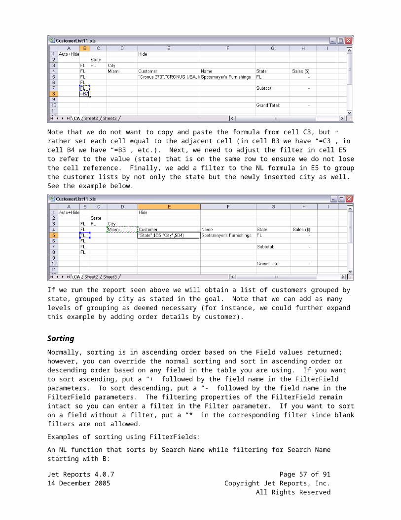
Date FunctionsFive date related functions in Excel make working with dates much easier. The functions are:

=Date(Year, Month, Day)

=Day(Date)

=Month(Date)

=Year(Date)

=Text(date, format)

To find the first day of the month from a date entered in D4, you could enter the following formula:

=Date(Year(D4), MONTH(D4), 1)

Since dates are stored in Excel as integers, you can find the last day of the month from a date entered in D4 with the following formula:

=Date(Year(D4), MONTH(D4)+1, 1)-1

Since you can disassemble a date easily into the Year, the Month and the Day, it is also easy to calculate the start of the year for the date in D4 with the following formula:

=Date(Year(D4), 1, 1)

If your fiscal year started in July instead of January, the formula is similar. The IF formula in the Year parameter determines if the start of the fiscal year is the same as the calendar year (i.e. Sept 6, 2003 is in the 2003 Fiscal Year), or if you need to subtract 1 from the calendar year (May 15, 2003 is in the 2002 Fiscal Year):

=Date(If(Month(D4)<7,Year(D4)-1, Year(D4)),7, 1)

To build a date range from two dates, use the NL function. If the start of the month was in cell D4 and you wanted to calculate a filter for the whole month, the formula for the date range would be:

=NL (“DateFilter”,D4, Date(Year(D4), MONTH(D4)+1, 1)-1)

The function above looks complicated, but it is just an NL function, with the end of month formula listed above.

Excel Addressing ModesExcel has three addressing modes: relative, absolute and mixed. Absolute addresses will reference the same cell no matter where the reference is moved or copied in a worksheet. For example, when you copy the formula =$A$3 from B3 to C5, it will still read =$A$3. A relative address will reference the same cell in relation to any cell where it is copied. For example cell B3 is one cell to the right of A3, so when you copy the formula =A3 from B3 to C5, it will now read =B5. Mixed mode addressing contains one relative coordinate and one absolute coordinate, for example $A3 or A$3. Mixed mode addressing is extremely useful for quickly generating reports using NL and NF functions. There are several examples of the use of mixed mode addresses in the Spread Company Income Statement report that comes with Jet Reports.

Excel Date ProblemsIf Jet Reports is returning dates (i.e. Posting Dates or Period Start dates) four years ahead of the year that you are filtering for, you may have your workbook set to use the 1904 date system. In Office 2000 and XP, you can change the date setting in the Tools/Options/Calculation menu. Turn off the check box next to the “1904 date system” setting.

If you have your Windows Regional Settings configured to treat dates as MM/DD/YYYY and you are using dates in Jet Reports as DD/MM/YYYY, you will either get unexpected results, or you will get #VALUE, depending on which dates you are specifying. You can create the same sort of problem with some database servers that have a built in date formula specification. For some database servers, the date format can be configured independently from Windows, so you need to know what date format the server is set to.


All Rights Reserved

Formatting a Cell as TextIn the current version of Jet Reports, setting the Number format of a cell to Text can cause problems. When you format a cell as Text, the formula itself becomes the value of the cell and Excel does not evaluate it. Since Jet Reports assumes that Excel will evaluate any formula entered into a cell, this can be a problem. It is best not to set the Number format of a Cell as Text.

Named RangesAny range in Excel can be associated with a name that can be used to reference that range anywhere in the workbook. Naming ranges is particularly useful if you are referencing a particular cell, such as a Start Date on the Options sheet, in several worksheets. Entering a name like “StartDate” in the Name Box in the upper left corner of the Excel screen makes referencing the date cell much easier as you design the rest of the report. You must press Enter after typing in the name, or Excel will not save it. There is one caveat to using Named Ranges which occurs when you are nesting formulas as parameters for other formulas. An example of this is the If statement below that outputs “More” if the sum of B5:B10 is greater than 10 and “Less” otherwise:

=If(Sum(B5:B10)>10,”More”,”Less”)

The cell references in the above formula cannot be named ranges, they have to be cell references like they are now since the Sum formula is nested in the If formula.

Now() and Today()The Now() and Today() functions are called volatile functions and can cause problems in Jet Reports because they recalculate each time there is a change in the worksheet. Jet Reports makes large numbers of changes to the workbook while it runs and each of those changes can cause a recalculation of the entire worksheet if you have a volatile function on the same worksheet. To avoid issues with volatile functions use the NL command with the Eval option. Please see the NL reference section above.

Protected WorksheetsIf you protect a worksheet in a workbook using the Excel “Protect Sheet” feature, Jet Reports will not be able to generate a report. Jet Reports will automatically protect locked worksheets (worksheets that have “Auto+Report+Lock” in cell A1) after a report is generated and will automatically unprotect locked worksheets with Jet/Design.

Using Filter Ranges in ExcelAlways enclose in quotes any ranges containing “..” that you type directly into a formula or into a parameter with the Excel function wizard. Without quotes, Excel may interpret your range as a set of values from the worksheet. For example, if you enter “49950..59950” including the quotes, Excel will interpret the filter as a simple text string. Without the quotes, 49950..59950 means all the values in rows 49950 through 59950. Since each row has 256 cells, this is an array of 2,560,000 cells. In this example, if you omit the quotes, Excel will go into a very long calculation. Usually the only way to stop this calculation is to end the process. Consult your IT expert for instruction on how to end a process on your computer.

This functionality of Excel has nothing to do with Jet Reports. However, Jet Reports users are more likely to accidentally enter a range that causes Excel to perform a long calculation because of the way ranges of values are entered using “..” as a range. Since the range calculations are a basic feature of Excel and there is no way for Jet Reports to change this behavior.

If a formula references a cell that contains a range with “..” you do not need to type the quotes into the cell. The quote are only required when you put the range directly into a function parameter.


All Rights Reserved

Using Navision Ranges in ExcelAlways enclose in quotes any ranges containing “..” that you type directly into a formula or into a parameter with the Excel function wizard. Without quotes, Excel may interpret your range as a set of values from the worksheet. For example, if you enter “49950..59950” including the quotes, Excel will interpret the filter as a simple text string. Without the quotes, 49950..59950 means all the values in rows 49950 through 59950. Since each row has 256 cells, this is an array of 2,560,000 cells. In this example, if you omit the quotes, Excel will go into a very long calculation. Usually the only way to stop this calculation is to end the process. Consult your IT expert for instruction on how to end a process on your computer.

This functionality of Excel has nothing to do with Jet Reports. However, Jet Reports users are more likely to accidentally enter a range that causes Excel to perform a long calculation because of the way ranges of values are entered using “..” in Navision. Since the range calculations are a basic feature of Excel and there is no way for Jet Reports to change this behavior.

If a formula references a cell that contains a range with “..” you do not need to type the quotes into the cell. The quote are only required when you put the range directly into a function parameter.

Avoiding Unwanted Excel AutoCorrectionThough Excel’s AutoCorrect feature can be very helpful at times, it can also be a bit of a nuisance when it comes to formatting. For instance, let us assume that cell B2 is formatted as Currency and B3 is formatted as a Percentage. In cell B4 we type ‘=B2*B3’ in order to obtain the product of the two values. With Excel AutoCorrection turned on, the cell is automatically formatted as Currency. Though this may typically be what we want, let us say that in this instance we would like to apply the Accounting format to the product. Excel will allow us to do this until the cell is recalculated. This becomes a problem, for instance, when a Replicator expands, because during the expansion a recalculation occurs throughout the entire workbook. This may cause you to think that Jet Reports is reformatting you workbook, while in fact it is an Excel feature that is causing the grief.

If you find yourself in this situation, you can attempt to turn off this feature by selecting ‘Tools/AutoCorrect Options’ in Excel. Select the ‘AutoFormat As You Type’ tab and make sure the ‘Include new rows and columns in list’ check box is deselected. Please note that for certain types of formatting there is nothing that can be done about Excel reformatting.


All Rights Reserved

Publishing with AutoPilot

OverviewAutoPilot allows workbooks saved in an input directory to be refreshed and saved to an output directory. The workbooks can be saved as converted workbooks or as web pages. By using Windows Task Scheduler, AutoPilot can automatically create updated workbook and web pages. When AutoPilot runs, it opens each workbook in the input directory. Depending on the mode specified on the command line, either it saves refreshed and converted workbooks to the output directory, or it saves Web Pages to the output directory.

Command Line ParametersAutoPilot determines what action to take based on command line parameters. The parameters follow the program name. AutoPilot recognizes the following command line parameters: /M, /I, /O, /D, /E, /X, and /P.

Parameter Action

/M Sets the mode. (VALUES, UPDATE,…)

/I Specifies the input directory or a particular report.

/O Specifies the output directory where the report(s) will be saved.

/D Turns on debug mode. You must specify a text file where the debug file will be saved. When AutoPilot runs Excel will open and errors and status will be stored in the debug file.

/E Emails the report(s) to the email addresses in the specified Excel range or a semicolon separated list of email addresses. Does not work with in SIMPLEWEB mode.

/X Creates and runs a batch file from the specified Excel range.

/P Starts the list of named range replacements. This must be last in the command line.

Here is how to setup the command line:

AutoPilot /M <Mode> /I <Input Directory> /O <Output Directory> /D <Debug File Path> /E <Range or list of email addresses> /X <Range> /P <Range1> <Value1> <Range2> <Value2> …

There must be a space between each command line item above: before and after /M, /I, /O, /D, /E, /X, and /P. If the input or output directory or any Range or Value has a space, it must be enclosed in quotes. The /P parameter must be last.

/XOften times when running AutoPilot you wish to update the batch file dynamically. This is not always easily done using DOS commands. However, dynamically updating Excel spreadsheets is much easier. /X allows you to write your batch files in Excel so you can use the power of Jet Reports and Excel functions instead of DOS commands to dynamically update your batch files.

When using /X, AutoPilot will run your report as normal. The “/X” parameter will then create and execute a temporary batch file from the specified named range in Excel. Each row in the named range will be a single line in the batch file. The columns in the range will be concatenated (separated by a space) to construct a line in the batch file.

This temporary batch file can be used to run another Jet Report via AutoPilot. If the specified named range does not exist in the report or reports specified in the input directory then a batch file will not be created or executed.


All Rights Reserved

/E/E automates the email distribution of your Jet Reports. When using /E, Autopilot will run your report as normal. It will then email the finished report to all of the specified email addresses. You can specify the list of email addresses on the command line in two ways.

First, you can specify an Excel named range that contains them. The named range can be any number of cells but must only contain one email address per cell. In this case, since the report is run prior to sending the email, the list of email addresses can be created using Jet Reports formulas giving you the ability to email the report based on a condition within the report. For example, you could conditionally hide or show an email address based on a G/L account balance in the report. If the balance of the account balance fell below a certain amount, the report would then be emailed to the CFO.

Alternatively, you can specify a semi-colon delineated list of email addresses on the command line itself. Please note that JetReports does not have the capability to check the validity of each address, so you will want to be careful to enter them correctly.

AutoPilot ModeMode Action

UPDATE Open workbook; Jet/Report; Save workbook in Output folder.

CONVERT Open workbook, Jet/Report; Jet/Publish/Convert Jet Formulas to Values (which saves the formula in the cell command and creates a drilldown hyperlink whenever “drilldown” is in the cell comment); Save workbook in Output folder.

This mode was originally provided to allow non-designers to view Jet Reports and is included for prior version compatibility. In the current version, the recommended way to allow non-designers to view Jet Reports is to design the report for Report Viewers and use the UPDATE mode. The VALUES mode is another good alternative.

SIMPLEWEB Open workbook; Jet/Report; Jet/Publish/Convert Jet Formulas to Values (which creates a drilldown hyperlink whenever “drilldown” is in the cell comment); Create subfolder in Output folder with workbook name; In this subfolder, save an html file for each sheet in the workbook.

VALUES Open workbook, run the report then convert all formulas to values and save workbook in Output folder. We recommend that you use +Values in cell A1 and the Update mode to achieve the same results.

Updating Report OptionsIf the workbook has single cell named ranges, AutoPilot can replace the contents of the named range. This allows AutoPilot to update report options. Follow the /P parameter with <Named Range> <New Value> pairs. Put a space between the Named Range and the New Value. If either includes spaces, enclose in quotes. You can include as many pairs as needed. If the named range does not exist in a workbook, it is ignored. Below are some example AutoPilot command lines:

AutoPilot /M UPDATE /I “C:\Input” /O “C:\Output” /P “DateFilter” “9/1/02..9/30/02” “Sales” “10000..”

AutoPilot /M SIMPLEWEB /I “C:\Daily Reports” /O “C:\Inetpub\Intranet\Daily Reports”

AutoPilot /M VALUES /I “C:\My Documents\Monthly” /O “C:\My Document\Monthly\ValuesOnly”

Command Line SubstitutionsThe input and output directories can contain date and time tags that will be replaced with current date and time elements. The follow tags are available:


All Rights Reserved

Tag Result

%YEAR% Current year, four digit

%MONTH% Current month, two digits

%DAY% Current day of the month, two digits

%HOUR% Current hour, 2 digits, 24 hour clock

%MINUTE% Current minute, 2 digits.

Note: If you are using the command line substitutions listed above in a batch file, you will have to use %% instead of % on either side of the tag. The %% is necessary because %NAME% in a batch file is also used for substitution, so %YEAR% will be evaluated by command.com before Autopilot ever runs.

The date and time substitutions are based on the date and time that AutoPilot starts. For example,

AutoPilot /M SIMPLEWEB /I “C:\Statistics” /O “C:\InetPub\%Year%-%Month%-%Day% %Hour%”

If the AutoPilot started at 10PM on July 23, 2003 the output directory from the above command line would be “C:\InetPub\2003-07-23 10”.

Using Windows Task SchedulerTo run AutoPilot on a schedule, use the Windows task scheduler. You need to use Windows 2000 or Windows XP Professional. You must set AutoPilot to “Run As” a user that has Excel and Jet Reports installed and properly configured. If you are not using Windows Authentication, the user name and password for Navision must be saved in the options. For better security, Windows Authentication is recommended.

AutoPilot SecurityYou should use Windows security to properly secure both the input and the output directories used with AutoPilot. Users that do not have at least the same permission or higher as the user in the “Run As” of the AutoPilot task scheduler should not be allowed to save workbooks to the input directory. Users that are not permitted to see the results should not be able to read files from the output directory.

TestingBefore saving a worksheet in the AutoPilot input directory, you should login as the user specified in the “Run As” of the task scheduler, open the workbook from the input directory, and choose Publish, Convert. Then use Save As to save the file to the output directory. If this is successful, AutoPilot should be able to create the output files. If you have trouble with a workbook, you should try this test to diagnose the problem.

Workbook Setup for AutoPilotWorkbooks in the Input directory should contain Jet Formulas. If you convert the Jet Formulas to values for workbooks in the Input directory, the worksheet will not refresh. If cell A1 of the first worksheet in the workbook does not contain “Report”, AutoPilot will automatically call Jet/Report.

AutoPilot will run faster if the workbook is saved in Design mode. This is automatic when “Report” is in cell A1 of the first worksheet. However, “Report” in cell A1 will also start a complete refresh when the workbook is opened. This makes opening the workbook to make changes to the report design slower.

Web Page Creation FormatWhen AutoPilot runs in SIMPLEWEB mode, a new directory is created for each workbook in the input directory. The name of the directory is the same as the name of the workbook. For each sheet in the workbook, an HTM file is created in the workbook directory. The filename is the same as the name of the sheet.


All Rights Reserved

If you want a drilldown hyperlink on the web page for a cell, put “drilldown” in the cell comment. To use the hyperlink, the user must have Navision installed on their computer and they must be able to access the Navision server.

User Access to Created Web PagesYou can setup navigational pages so users can more easily find the web pages created by AutoPilot or users can just use Windows explorer to find the HTM files and open them. If users have Navision access, they can click on the drilldown to Navision hyperlinks and Navision will automatically open to display the source of the information on the web page.


All Rights Reserved

Version Change HistoryChanges in Version 4.0.X

Major speed improvements.

Added the Jet Toolbar.

Added the Jet Scheduler.

o Schedule reports directly from Excel.

o Email reports to one or more users.

o Send alerts via email based on report results.

o Optionally extract recipient email addresses from database.

Added ability to convert Jet Reports to simple workbooks.

o Convert Jet formulas to values.

o Preserve all other Excel formulas.

o Create unprotected, editable reports.

o Preserves hidden rows, columns, sheets so report can be refreshed.

o Provide Revert ability to restore changes accidentally lost by report refresh.

o Designers simply put “Auto+Hide+Values” in cell A1 to turn on this ability.

Introduced the Advanced Designer for all Navision versions 2.60 and later.

o Provides additional schema related information such as table/field relationships and CalcFormulas for FlowFields.

o Provides direct access to Navision Help for all available tables and fields.

Improved ability to summarize and structure reports by collapsing all Excel Data Groups after report run.

Compensated for various stability issues related to Excel 2000.

Simplified Progress Window to improve speed.

Added support for Slovenian and Spanish.

Added array manipulation features to the NL function.

Improved sorting speed.

Modified sorting so that the sort order matches Navision in most cases.

Added a new, faster method of filtering data across tables.

Improved filtering one table based on values in another table with “Filter” as a “What” argument of the NL function.

Disabled Navision’s field and table name auto-completion

Minor menu adjustments and bug fixes

Changes in Version 3.7.4

Added cross reference sheet for all supported languages

Minor bug fixes


Increased speed for Advanced Dimensions


All Rights Reserved

Minor bug fixes


Increased overall speed and stability

Added support for Navision 4.0

Added support for Turkish language

Minor bug fixes


Added new options to the Jet Designer including whether or not the Designer is displayed upon selecting Jet/Design, the option to have the Designer window stay on top of the Excel window, and the option of having the Designer window be transparent.

Added a ‘fit’ tag, which will automatically fit the specified column or row based on the largest item that it contains

Added upgrade functionality to the installer. You no longer need to remove an old version of Jet Reports to upgrade to a new version.


Added the Jet Designer which replaces the Jet Wizard. To see it, just choose Jet/Design. You can drag fields into Excel to automatically insert retrieval formulas. You can right click on a name and Send it to Excel just as if you had typed it. You can use the Designer to find tables, fields, values, and function options while you are in the middle of entering formulas or using the Excel Paste Function wizard.

Added an Auto Debug option, which automatically selects the first cell with #VALUE and shows the Jet/Debug message after a report is generated. You can disable this feature.

The limit of four decimal places for Navision numeric fields has been removed for executable versions 2.60e or later. Jet Reports now returns all the decimal places stored in Navision.


Added Advanced Dimensions as Virtual Fields to tables that have Advanced Dimensions. This allows very easy filtering on and retrieval of Advanced Dimension values. Just treat the Advanced Dimension code as if it were a field.

Enhanced the NL function to accept an array in the Table argument when the “What” argument is “Rows”, “Columns” or “Sheets”. A row, column, or sheet is created for each element of the array.

Added the ability to use an array for a Filter. A record is selected if any element of the array matches. Of course, all the other “non-array” filters have to match too. See details below under Array Filters.

Added “AllUnique” as a “What” argument of the NL function which allows the NL function to generate array filters. See details below under Array Filters.


Added 14 new example reports including Summary Customer and Vendor Aging, Pareto Chart, and Item Sales List by Date

Significantly enhanced performance for reports with nested replicators

Corrected issued in 3.5.1 that caused Jet Reports to fail to recognize when sum index would improve calculation speed.

Enhanced AutoPilot to allow a file name in the /I argument. To specify a file, just add the name of the file after the path. Wildcard characters “*” and “?” are allowed.

AutoPilot now creates entries in the application log

Added a “Values” mode to AutoPilot which converts all formulas to values before the workbook is saved

Minor enhancements and bug fixesJet Reports 4.0.7 Page 65 of 6714 December 2005 Copyright Jet Reports, Inc.

All Rights Reserved


Added support for a single report to pull data from selected multiple versions of Navision at the same time. This feature requires Windows 2000, Windows XP, or later. Version 3.5.1 can support the currently installed version plus versions 2.6e, 2.6f, 3.01b, 3.10a, and 3.60.

Added Fast Columns support. Removed option for Fast Rows. Now Fast Rows and Fast Columns are always on. Enhanced ability to interrupt a report during calculation.

Added support for Navision captions. To use captions, the user must export the language module and then enter the path for the language module in Jet/Options. Jet Reports 3.5.1 will do internal sorts based on the active language’s locale settings. See notes in installation documentation.

Enhanced AutoPilot to add a debug mode and to properly handle relative paths. In debug mode, report generation is visible and error messages are sent to the screen.

Enhanced NL function to insert pictures into a report. Pictures can come from a file or from the Navision database. The picture to insert and the picture size can be calculated.

Added ascending and descending sorting by multiple fields (without required a Navision database key). When the NL function is returning unique values, the default sort can be changed.

Added ability to exclude Closing Dates. Just prefix the date filter with “<>C&” and closing dates will be excluded. Added an ExcludeClose parameter to the GL Function.

Added ability to automatically ignore all special filter characters and search for an exact match of the contents in the filter. Just prefix the filter with “@@”.

Added a special FilterField value “LIMIT=“. Put the maximum number of records in the Filter. When used in conjunction with sorting, you can create Top X lists like Top 10 Customers by Sales.

Added Jet Reports license expiration warning. This is primarily for dealers. End user licenses do not normally expire. Jet Reports 3.5.1 will now work with a Navision license file that is issuing a License expiring soon warning.

Corrected problem that occurs when the Regional Setting for the list separator is a semicolon instead of a comma

Page breaks that occur with the copied region of an NL function are now copied too.

Corrected problems with merged cells, which now expand “logically” when rows or columns are copied

Minor bug fixes and menu adjustments


Added support for a single report to pull data from more than one Navision database or server. Default connection is specified in Jet/Options. Added Connection field to the GL function. To override the default connection in an NL function, put “Connection=“ in a FilterField and the connection name as defined in Jet/Options in the corresponding Filter. Multiple server connections and a single local database can be use on the same report.

Added new Options including a Fast Row Option for faster reports with less frequent screen updates

Jet Options can be stored in an external file so that multiple users can share the same options. Options and Jet License files can be stored on a shared network folder. A custom installation can be defined with custom default options. See Installation Guide for details.

AutoPilot enhanced to update report options. New mode added to simply update report

Added documentation on how to launch Jet Reports from Navision

Changes in Version 3.4

Added support for “Auto+Hide+Lock” tag in cell A1 of a worksheet which causes the formulas to be locked after Jet/Report is finished updating the report. Worksheets with this tag are automatically protected to prevent accidental changes. A worksheet that is locked does not contain any formulas so it can be opened


All Rights Reserved

by Excel users without Jet Reports installed. Locked worksheets open fast because there are no formulas to evaluate.

Added support for Viewers. A report Viewer can change report options and update the report using Jet/Report but can not use any other features of Jet Reports. Viewers may not enter Jet formulas into worksheet cells. When Viewers design reports for use, all worksheets must be locked except worksheets that contain report options.

Improve speed and diagnostic error messages


Changes in Version 3.3

Enhanced NL function. Added ability to automatically create worksheets, copy multiple columns or rows at a time, and return sorted, unique values for a field.

Added compatibility with Navision version 1.2 and later. Drilldown still requires 3.01b executables.

Added Publishing support. Jet Formulas can be converted to values. Drilldown can be retained after conversion by putting “Drilldown” in cell comment. Converted Jet Formulas can be restored. Excel users without Jet Reports can view converted worksheets and still use drilldown.

Added AutoPilot program to support scheduled Excel and Web publishing. Using Windows Scheduled Tasks, AutoPilot can automatically create converted Excel worksheet and Web pages. Drilldown can be made available from Web pages.

Added conditional row and column hiding

Add rule that filters may not be blank. Use “*” to indicate any value is allowed. This may impact reports where previously a blank was use in a report option to indicate all. This change allows Jet Reports to improve calculation speed for some reports.

Change function wizard to defer calculation until the entire formula is entered and accepted. Before, partially entered functions trigged slow calculations in some cases.

Increase speed of some NL function calculations by as much as 20x

Changed NL function calculation in Design mode to return first record found. Properly sorted values are returned in report mode. This speeds responsiveness in Design mode.



All Rights Reserved