Embed Size (px)
Citation preview

Jersey Calf Management, Mortality, and Body Composition.
Scott Shelton Bascom
Dissertation submitted to the Faculty of Virginia Polytechnic State
Institute and State University for partial fulfillment of the requirements
for the degree of
Doctor of Philosophy
in
Animal Sciences
Robert E. James, Chair
Ernest P. Hovingh
Michael L. McGilliard
Carl E. Polan
John C. Wilk
November 18, 2002
Blacksburg, VA
Copyright 2002, Scott S. Bascom
(Keywords: Calves, Survey, Body Composition, Milk Replacer,
Mortality)

(Abstract) Jersey Calf Management, Mortality, and Body Composition.
Scott S. Bascom
In experiment one, week old Jersey bull calves (n=39) were assigned to one of four
diets: 21/21 (n=8), 27/33 (n=8), 29/16 (n=9), MILK; or a baseline sacrifice group
(n=6). Diets 21/21, 27/33, and 29/16 were milk replacers containing 21, 27, or 29%
CP, and 21, 33, and 16% fat, respectively. Diet 21/21 was fed at 15% of BW. Diets
27/33, 29/16, and MILK supplied 180g CP/d. Calves were fed 4 wk. Weight, hip
height, wither height, heart girth, and body length were measured weekly. Weekly
plasma samples were analyzed for PUN, NEFA, and glucose. Calves were processed
to estimate body composition. Feed efficiency and ADG were greatest for calves fed
MILK, least for calves fed 21/21, and intermediate for calves fed 29/16 and 27/33.
Calves fed 27/33 or MILK had the greatest gains of fat and percentage fat in the empty
body. Body fat percentage of calves fed 29/16 or 21/21 was not changed by diet.
Performance of calves fed 27/33 and 29/16 was similar except that calves fed 29/16
were leaner and calves fed 27/33 had a propensity for elevated NEFA. Feeding 180g
of CP in the MR was beneficial to calf performance compared with diet 21/21.
In experiment two, tissues from a subset of calves [21/21 (n=4), 27/33 (n=5), 29/16
(n=5), MILK (n=3), baseline (n=2)] were scanned using dual energy x-ray
absorptiometry to estimate mass, fat, CP, and ash. Liver, organ, and carcass mass by
DXA were correlated to scale weights (R2= 0.99, 0.62, and 0.79, respectively). DXA
was a poor predictor of percentage fat, CP, and ash (adjusted R2 <0.10).
Experiment three determined level of calf mortality in the United States; and identified
opportunities to reduce mortality. Herds (n=88) were representative of the US Jersey
population. Production averaged 7180 ±757 kg milk annually. Herds averaged 199
births annually. Mortality was 5.0% from birth to 24 h (M24) of life and 6.7% from
24 h to 3 mo of life (M3). Level of mortality (M24) was highest in herds that calved
on pasture. Lower levels of mortality (M3) were associated with use or maternity pens
and earlier weaning

iii
Acknowledgements The author would like to thank Kristin Burkholder, Autumn “Dee” Guyton, C. Shai
Huffard, Coleen Jones, Peter Jobst, Beth Keene, and Leanne Wester for their help with
the calf feeding trial. I am grateful to Harold Nester, Chuck Miller, Curtis Caldwell,
and the Virginia Tech farm crew for their assistance. I appreciate the help and
assistance I received from Charles “Chip” Aardema, Jr. and the Virginia Maryland
School of Veterinary Medicine in processing my calves.
Thanks to Wendy Wark, Patricia Boyle, and Laura Coffey for providing assistance in
conducting my laboratory work. Phoebe Peterson went beyond the call of duty in
helping process my paper work and keeping Dr James straight!
I am grateful to Dr Michael Van Amburgh, Debbie Ross, Matt Meyer, Dr “Denny”
Shaw, and the staff at Cornell University for their assistance in processing, analyzing,
and determining the composition of my calves.
This project would not have been possible without the financial support of Land
O’Lakes and the American Jersey Cattle Association. The author is particularly
grateful to Dr Mike Fowler at Land O’Lakes for his technical expertise. Cari Wolfe,
Neal Smith, and Erick Metzger provided support and expertise in collecting the Jersey
calf management data.
I also would like to express my gratitude to the numerous Jersey breeders who
provided data for the calf management survey. Thanks to James Huffard, and the
staff at Huffard Dairy farms for providing Jersey bull calves.
Thanks to Dr James, Dr Hovingh, Dr Polan, Dr Wilk, and Dr McGillard for serving as
my advisory committee and training me as a scientist.

iv Last but certainly not least, I would like to express my sincere gratitude to Stacy
Wampler for the many hours of assistance she provided in numerous aspects of this
project. Few students are more devoted and dedicated than Stacy, and it was a
pleasure working with you.

v Table of Contents (Abstract) ....................................................................................................................... ii Acknowledgements....................................................................................................... iii Table of Contents............................................................................................................v List of Tables .............................................................................................................. viii List of Figures .................................................................................................................x List of Appendices ....................................................................................................... xii Chapter One ....................................................................................................................1 Introduction.....................................................................................................................1 Chapter Two....................................................................................................................5
DIETS FOR PREWEANED CALVES .....................................................................5 Growth and development ........................................................................................5 Milk composition as a means of estimating nutrient requirements of the neonate.6 Digestive anatomy and physiology of the preweaned calf....................................12 Estimates of the nutrient requirements of calves ..................................................13 Energy requirements and the role of dietary fat...................................................13 Protein requirements in the calf and the role of dietary protein ..........................17 Development and history of milk replacers ..........................................................19 Intensified rearing of calves..................................................................................23 Rapid growth and heifer development ..................................................................29 Rapid growth and future milk yield ......................................................................30 Body composition analysis....................................................................................31 Whole body analysis of composition....................................................................31 Multi-compartment models of analysis.................................................................32 Common methods of analyzing body composition................................................34 Dilution .................................................................................................................34 Bioelectrical impedance........................................................................................35 Dual x-ray absorptiometry analysis of body composition ....................................37 What is the ideal body composition? ....................................................................40 Objectives..............................................................................................................42
Chapter Three................................................................................................................43 CALF MORTALITY SURVEYS..........................................................................43
Introduction...........................................................................................................43 Management factors..............................................................................................45 Colostrum and management of the newborn ........................................................46 Calf mortality and disease ....................................................................................47 Feeds and feeding .................................................................................................48 Housing .................................................................................................................50 Other considerations.............................................................................................51 Justification...........................................................................................................51 Objectives..............................................................................................................52
Chapter Four .................................................................................................................53 MATERIALS AND METHODS...........................................................................53

vi
CALF FEEDING TRIAL ....................................................................................53 Experimental procedure: ......................................................................................53 Animals: ................................................................................................................53 Diets:.....................................................................................................................55 Digestibility study: ................................................................................................57 Weekly measurements:..........................................................................................58 Blood samples:......................................................................................................58 Environmental conditions:....................................................................................58 Sacrifice procedure and body composition: .........................................................58 Analysis of tissue samples:....................................................................................59 Calculations ..........................................................................................................60 Statistical design and analysis:.............................................................................61
CALF MANAGEMENT SURVEY ........................................................................63 Herd selection .......................................................................................................63 Survey design and implementation .......................................................................64 Statistical analysis ................................................................................................64
Chapter Five..................................................................................................................65 INFLUENCE OF DIETARY FAT AND PROTEIN RATIOS ON BODY COMPOSITION OF JERSEY BULL CALVES. .......................................................65
Results and Discussion .........................................................................................65 Conclusions...........................................................................................................70
Chapter Six....................................................................................................................97 USEFULNESS OF DUAL X-RAY ABSORPTIOMETRY FOR ANALYZING COMPOSITION OF CALF TISSUES....................................................................97
Results and Discussion .........................................................................................97 Conclusions...........................................................................................................98
Chapter Seven .............................................................................................................111 JERSEY CALF MANAGEMENT PRACTICES IN THE UNITED STATES .................111
Results and Discussion .......................................................................................111 Conclusions.........................................................................................................120
Chapter Eight ..............................................................................................................129 CONCLUSIONS .............................................................................................129
Conclusions.........................................................................................................129 Synthesis..............................................................................................................130
REFERENCES................................................................................................132 Appendix A.................................................................................................................147 Assignment to Treatments ..........................................................................................147 Appendix B .................................................................................................................148 Sample Body Composition Calculation......................................................................148 Appendix C .................................................................................................................152 Jersey Calf Management Survey ................................................................................152 Appendix D.................................................................................................................160 Statistical Models........................................................................................................160

vii Appendix E .................................................................................................................171 Development of a milk replacer for Jersey calves ......................................................171 Vita..............................................................................................................................177

viii List of Tables
Table 2.1. Composition of milk of various species………………………………..8
Table 2.2. Composition of milks of five breeds of dairy cattle……………………9
Table 2.3. Effect of dry matter composition and feeding method on milk replacer
consumption and body weight gain in calves………………………...11
Table 2.4. Effect of fat level in a 22% protein milk replacer on growth, feed
conversion and fecal score…………………………………………....16
Table 2.5. Energy and Protein allowable gains for a 22.7 kg calf fed…………...19
Table 2.6. Chemical composition of milk byproducts…………………………...21
Table 2.7. Crude protein digestibility of milk replacers containing various protein
sources………………………………………………………………...22
Table 2.8. The effect of varying the level of intake and crude protein on feed
efficiency and body fat deposition……………………………………27
Table 2.9. The influence of protein levels in milk replacers on growth and
performance of male Holstein calves…………………………………27
Table 2.10. Content of the gross chemical components and energy in the digesta-
free body weight gains according to dietary protein concentration…..29
Table 3.1. Causes of death in preweaned calves…………………………………44
Table 3.2. Factors associate with mortality in preweaned calves………………..49
Table 4.1 Diet specifications…………………………………………………….56
Table 5.1. Diet specifications………………………………………………….…73
Table 5.2. Total nutrient intake and performance of calves by diet……………...74
Table 5.3. Weekly heart girth, hip height, and weight…………………………...75
Table 5.4. Weekly body length and wither heights………………………………75
Table 5.5. Nutrient retention and digestion………………………………………76
Table 5.6. Weekly water intake…………………………………………………..76
Table 5.7. Gross energy content of body components…………………...….…..77
Table 5.8. Composition of empty body…………………………………………..77
Table 5.9. Changes in body composition………………………………………...78

ix Table 6.1. Diet specifications………………………………………………….....99
Table 6.2. Total nutrient intake and performance of calves………………….....100
Table 6.3. Composition of tissues as estimated by DXA……………………….100
Table 6.4. Composition of tissues estimated by DXA or chemical analysis…...100
Table 7.1. Characteristics of the herds surveyed by region of country…………122
Table 7.2. Calf mortality and management of newborns……………………….123
Table 7.3. Correlations between management and calf mortality………………124
Table 7.4. Summary of nutrition and feeding management…………………….124
Table 7.5. Summary of health and reproductive management………………….125
Table 7.6. Primary calf feeder…………………………………………………..126
Table 7.7. Coefficients to predict calf mortality in the first 24 hours of life…...127
Table 7.8. Coefficients to predict calf mortality in the first 3 months of life…..127

x
List of Figures
Figure 2.1. Steps in processing the associated byproducts used in manufacture of
milk replacers…………………………………………………………21
Figure 2.2. Body weight on day 1 to 29 of Holstein and Jersey calves…………...24
Figure 2.3. Efficiency of feed conversion………………………………………...25
Figure 2.4. Models of body composition………………………………………….33
Figure 5.1. Average daily weight gain by diet……………………………………79
Figure 5.2. Total weight gained by diet…………………………………………...80
Figure 5.3. Weekly weight by diet………………………………………………..81
Figure 5.4. Weekly hip heights by diet……………………………………………82
Figure 5.5. Weekly body length by diet…………………………………………..83
Figure 5.6. Weekly wither heights by diet………………………………………..84
Figure 5.7. Weekly heart girths by diet…………………………………………...85
Figure 5.8. Weekly plasma urea nitrogen by diet…………………………….…...86
Figure 5.9. Weekly blood glucose by diet………………………………………...87
Figure 5.10. Weekly NEFA by diet………………………………………………...88
Figure 5.11. Percent fat in empty body by diet……………………………….……89
Figure 5.12. Composition of empty body weight gain……………………………..90
Figure 5.13. Empty body composition by diet……………………………………..91
Figure 5.14. Weekly average fecal score by diet…………………………………..92
Figure 5.15. Distribution of medication days by diet………………………………93
Figure 6.1. Chemical analysis of ash in carcass versus DXA bone mineral
content……………………………………………………………….102
Figure 6.2. Chemical analysis of protein in carcass versus DXA lean tissue……103
Figure 6.3. Chemical analysis of water in carcass versus DXA lean tissue……..104
Figure 6.4. Chemical analysis of fat in carcass versus DXA fat……………...…105

xi Figure 6.5. Chemical analysis of water in blood and organs versus DXA lean
tissue…………………………………………………………………106
Figure 6.6. Chemical analysis of protein in blood and organs versus DXA lean
tissue…………………………………………………………………107
Figure 6.7. Organ mass versus DXA estimate of organ mass…………………...108
Figure 6.8. Liver mass versus DXA estimate of liver mass……………………..109
Figure 6.9. Carcass mass versus DXA estimate of carcass mass………………..110
Figure 7.1. Interaction between volume of colostrum fed in first feeding and the
age calf starter was offered………………………………………….111

xii
List of Appendices Appendix A Assignment of calves to treatments....................................................147
Appendix B Sample body composition calculations……………………………...148
Appendix C Jersey calf management survey……………………………………...152
Appendix D Statistical models……………………………………………………160
Appendix E The development of a milk replacer for Jersey calves……………....171

1
Chapter One
Introduction
Interest in Jerseys and Jersey calves appears to be increasing. The American Jersey
Cattle Association (AJCA) has reported a record high number of registrations; more
than 70,000/yr, over the last 2 yr indicating an increase in participation in Jersey breed
programs. Participation in breed programs serves as an indirect indicator of a strong
demand for Jersey cattle, which increases the market value of Jersey calves.
Therefore, as demand for Jersey cattle increases more emphasis is placed on practices
that enhance calf performance and/or reduce calf mortality.
In 1992 and 1996, the National Animal Health Monitoring Service (NAHMS) released
the results of national surveys of calf management practices and mortality. The mean
death loss of calves between birth and weaning was reported to be 8.4 and 11.4% in
1993 and 1996, respectively. These surveys were comprehensive and represented
78% of the dairy herds in the US but only 2.4% of the herds surveyed were Jersey
herds. The Jersey calf is unique due to its smaller frame size, lighter birth weight, and
genetics. Therefore, the NAHMS surveys do not necessarily represent reliable
information on Jersey calves, and surveying management practice in Jersey herds is
merited.
In addition to surveying management practices, intensive feeding trials designed to
elucidate the specific nutrient requirements of Jersey calves might yield information
that could be used to design feeding programs specifically for Jersey calves. Recently,
intensified calf feeding programs have been developed for Holstein calves. These
programs are designed to improve feed efficiency, ADG, and promote lean tissue
growth. Calves fed intensive feeding programs are often encouraged to consume milk
replacer at 15% of their body weight. Feeding calves aggressively may result in
improvements in future milk yield. Researchers in Israel and Denmark reported

2 feeding black and white (Holstein or Holstein crosses) calves at or near ad lib intake
during the first 6 wk of life increased first lactation milk yield, decreased age at first
calving, and increased BW at calving. The mechanisms by which feeding calves
more liberally improves their lactation potential are unclear but may be related to
changes in mammary tissue development and lean frame size. The results of these
studies have led researchers to reconsider conventional calf feeding programs that
limit-feed milk to calves.
Special milk replacers formulations have been developed for use in intensified feeding
programs. These milk replacers are typically 28 to 30% CP and 16 to 20% fat.
Whole cows milk typically contains 25 to 30% CP on a DM basis. The nutrient
composition of these diets is designed to promote efficient gains in lean body tissue.
Therefore, the higher level of CP in milk replacers that are fed near ad lib intake
would appear to have merit. However, these programs may not be applicable to Jersey
calves due to breed differences in BW, frame size, and metabolic BW.
Objectives:
The objectives of the experiments described in this work were:
1) To examine the relationship between dietary protein and energy and growth,
body composition, protein retention, energy utilization, and feed efficiency in
Jersey bull calves.
2) To investigated the potential usefulness of dual energy X-ray absorptiometry to
estimate body composition.
3) To characterize management practices associated with calf mortality.
4) To identify differences in heifer management practices by level of milk
production.
5) To assess the relationship between region of the country, herd size, level of
production, and other management practices with calf mortality.
3
6) To identify opportunities for improvements in Jersey calf and heifer
management.
Organization
The first experiment was designed to address objectives that focused on the impact of
nutrition on body composition and growth. The second experiment was designed to
evaluate the effectiveness of DXA in evaluating body composition. The final study
was designed to focus on objectives that dealt with Jersey calf management and
mortality.
Chapter 2 is a discussion of the literature related to calf nutrition, body composition,
the impact of nutrition on body composition, and methods of evaluating body
composition in calves.
Chapter 3 contains a review of survey data that was collected to evaluate management,
nutrition, mortality, and other calf management practices on dairy farms in the United
States.
Chapter 4 is organized in two sections. The first section reviews the materials and
methods utilized in experiments 1 and 2 to evaluate growth and body composition of
calves fed differ levels of fat and protein. The second section details the materials
and methods used in surveying Jersey herds in the US to collect data on calf
management, nutrition, and mortality.
Chapter 5 discusses the influence of dietary fat and protein on body composition.
Chapter 6 examines the usefulness of DXA for evaluating composition in calves.
Chapter 7 describes the management of Jersey calves in the United States.

4
Chapter 8 summarizes the key findings in all experiments.

5
Chapter Two
Diets for Preweaned Calves
Growth and development
Growth and development are complex phenomena that begin at conception and
continue until maturation and are unique but interrelated. Batt (1980) defined growth
as quantitative changes in the body while development expresses qualitative changes.
More specifically, growth involves an increase in body size including increases in
BW, heart girth, volume, or stature. Development encompasses changes in shape,
conformation, or function of tissues. In a review of growth and development of
ruminants, Owens et al. (1993) explained the primary mechanisms of growth as 1)
hyperplasia, the accumulation of new cells; and 2) hypertrophy, the enlargement of
cells. Growth and development can be categorized into several unique periods
including prenatal, neonatal, prepubertal, pubertal, and post pubertal. Each of these
phases is distinct and involve metabolic processes that vary considerably as the animal
moves through these stages.
During prenatal development, all of the organism’s cells grow by hyperplasia, but
post-natally, the majority of growth occurs by hypertrophy (Owens et al., 1993). In
humans, cells divide 42 times before birth, but only five times from birth to maturity
(Batt, 1980). A similar observation has been made in rats. In late gestation, the
prenatal rat may increase the number of new cells produced by as much as 60% per
day; just prior to birth, the rate of new cells produced drops to 20%, and at puberty the
rate of new cell production is only 2% per day (Hafez and Dyer, 1969). The function
of cell division in adults is considerably different from prenates; in the mature animal
new cells are produced at a steady but slow rate to maintain cell numbers by replacing
cells that are lost (Hafez and Dyer, 1969).

6
The literature is replete with information regarding growth in various stages of life of
the bovine. However, the remainder of this treatise will focus primarily on nutritional
and management factors, and their effect on growth and development in the calf. The
definitions of growth provided previously explain this phenomenon in a broad sense,
but the following explanation of growth is narrower and more directly applicable;
“Growth and development occur in the neonate when the input of nutrients to the
organism is more than enough to make good the losses incurred in the dissipation
process. This excess fills out the organism through the building up of an elaborate
internal organization composed of cellular subunits. Materials and energy made
available for growth are used to produce new cells, to fill out old cells or to create
extracellular material like fat.” (Calow, 1978).
Milk composition as a means of estimating nutrient requirements of the neonate
All neonatal mammals depend on their dams to ingest and convert nutrients that are
not readily digestible by the neonate to a highly digestible source of nutrients, i.e.,
milk. The degree of reliance on lactation to provide nutrients varies considerably
from species to species. For example, the American Association of Pediatrics (1997)
discouraged weaning breast-fed human infants before 12 mo of age; on the other hand,
calves can be weaned successfully as early as 6 wk of age (Davis and Drackley,1998).
The difference in weaning age between species is related to the species ability to
consume nutrients from sources other than milk (Jenness, 1985). Studying the
nutrient composition of milk can provide valuable insight into the nutrient
requirements of the neonate during the period of its life when the dam’s milk is the
primary source of nutrition.
Jenness (1985) stated, “The biological function of milk is to supply nutrition and
immunological protection to the young mammal.” Therefore, understanding the
composition of milk is a logical starting point to understanding the nutrient needs of
the neonate. The composition of milk from several different species is shown in

7 Table 2.1. Species such as the dolphin, fur seal, and bear produce milk with a high
caloric density, which is achieved by synthesizing milk that contains a high
concentration of fat and a low concentration of lactose. These species live in habitats
that require them to expend a great deal of energy for maintenance. Maintenance
energy requirements are influenced by the physiological stage at birth, i.e., species
where the neonate becomes ambulatory soon after birth are less dependent on their
dams than species where the neonate does not become ambulatory soon after birth. In
the case of the dolphin and the seal, a high proportion of the neonate’s caloric intake is
expended to maintain a constant body temperature. On the other hand, species such
as the horse and the red kangaroo produce milk with relatively low caloric density, and
their milk has a low concentration of fat but a high concentration of lactose. The foal
is able to begin consuming roughages soon after birth and is less dependent on milk to
provide its caloric needs. The red kangaroo lives in a warm habitat, resides in its
dam’s pouch, and requires less energy for thermoregulation. Milk composition also
varies within a species (Table 2.2). Possibly, intra-species variation in milk indicates
differences in neonatal nutrient requirements of for different breeds. For example,
Jersey and Guernsey calves may have higher maintenance energy requirements and
thus require a more energy-dense diet than calves of the Holstein or Ayrshire breed, as
indicated by the breed differences in milk composition.

8
Table 2.1. Composition of milk of various species.
Percentage by weight
Species Water Fat Casein Whey Protein Lactose Ash Energy
(kcal/100g)
Red kangaroo 80.0 3.4 2.3 2.3 6.7 1.4 76
Human 87.1 4.5 0.4 0.5 7.1 0.2 72
Rabbit 67.2 15.3 9.3 4.6 2.1 1.8 202
Gray squirrel 60.4 24.7 5.0 2.4 3.7 1.0 267
Rat 79.0 10.3 6.4 2.0 2.6 1.3 137
Dolphin 58.3 33.0 3.9 2.9 1.1 0.7 329
Black bear 55.5 24.5 8.8 5.7 0.4 1.8 280
Fur seal 34.6 53.3 4.6 4.3 0.1 0.5 516
Indian elephant 78.1 11.6 1.9 3.0 4.7 0.7 143
Horse 88.8 1.9 1.3 1.2 6.2 0.5 52
Pig 81.2 6.8 2.8 2.0 5.5 1.0 102
Camel 86.5 4.0 2.7 0.9 5.0 0.8 70
Reindeer 66.7 18.0 8.6 1.5 2.8 1.5 214
Cow (bos taurus) 87.3 3.9 2.6 0.6 4.6 0.7 66
Cow (bos indicus) 86.5 4.7 2.6 0.6 4.7 0.7 74
Water buffalo 82.8 7.4 3.2 0.6 4.3 0.8 70
Goat 86.7 4.5 2.6 0.6 4.3 0.8 70
Sheep 82.0 7.2 3.9 0.7 4.8 0.9 102
Adapted from Jenness (1985).
While species and breeds vary in the concentration of many nutrients in their milk the
osmolality of milk is almost always maintained at 0.3 M, regardless of species or
breed (Jenness, 1985). The osmolality of blood is also 0.3 M. Similarities in the
osmolality of blood and milk are not coincidental. If a difference existed between the
osmolality of milk and blood, then an osmotic gradient would be created during
digestion and fluid would tend to flow between blood and milk in an attempt to
achieve equilibrium. If the osmolality of milk favored the flow of water from blood to
milk, then the electrolyte balance might be upset, which could result in dehydration.

9 However, the similar osmolality of blood and milk prevents the flow of fluid from
capillaries to the lumen of the intestine and thus prevents dehydration.
Table 2.2. Composition of milks of five breeds of dairy cattle.
Mean percentage by weight
Breed Total solids Fat Casein Whey protein Lactose Ash
Ayrshire 12.69 3.97 2.68 0.60 4.63 0.72
Brown Swiss 12.69 3.80 2.63 0.55 4.80 0.72
Guernsey 13.69 4.58 2.88 0.61 4.78 0.75
Holstein 11.91 3.56 2.49 0.53 4.61 0.73
Jersey 14.15 4.97 3.02 0.63 4.70 0.77
(Reinart and Nesbitt, 1956) as sited by Larson (1985).
Understanding the composition of milk allows one to make a qualitative assessment of
the nutrient needs of the neonate. Based on the composition of cow’s milk, we can
infer that calves require a diet that has approximately 3.9 to 5.0% fat, 3.2% CP, 4.6%
lactose, and less than 1% mineral on an as fed basis. However, one needs to consider
both the qualitative and quantitative aspects of neonatal nutrition when determining
the nutrient requirements of the neonatal calf. If a calf were nursing its dam, the
composition and the quantity of milk produced would provide the essential nutrients
that the calf requires to maintain its body and grow. Thus, examining the composition
of milk without considering the quantity of milk that the suckling calf consumes has
some shortcomings in defining the specific nutrient requirements of the calf.
Two factors determine the intake of milk in suckling animals: 1) level of milk
production of their dam; and 2) the ability of the neonate to consume milk. Milk
production of a cow is dictated by a wide variety of factors including her plane of
nutrition, environmental conditions, and genetics. Advances in nutrition,
management, and genetics allow most dairy cows to produce far more milk than their
calves can consume. Therefore, the ability of the calf to consume milk would be the
limiting factor if dairy calves were allowed to suckle their dams. Bar-Peled et al.

10 (1997) allowed Holstein calves to suckle their dams for 15 min twice per day until
they were 6 wk old; these calves had an average intake of 17 L/calf per day.
Lineweaver and Hafez (1969) fed Holstein and Hereford calves a milk replacer (MR)
that was reconstituted to either 6.5 or 19.5% solids. Milk replacer was delivered using
an automated nursing station, and calves were fed 4 times daily or allowed ad lib
intake. Calves allowed ad lib intake of the MR reconstituted to 19.5% solids had the
greatest DMI (3.25%) as a percentage of BW, greatest ADG, ADG as a percentage of
initial BW, and the greatest feed efficiency (Table 2.3). There is considerable debate
in the contemporary literature over the appropriate level of intake for dairy calves
which are raised as replacement heifers. Traditionally, dairy calves have been limit
fed the liquid portion of their diet to encourage the intake of dry calf starter. However,
more recently it has been suggested that preweaned calves may benefit by consuming
liquid at near ad lib intake (Drackley, 2001).
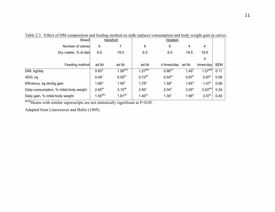
11 Table 2.3. Effect of DM composition and feeding method on milk replacer consumption and body weight gain in calves.
Breed Hereford Holstein
Number of calves 6 7 6 6 4 4
Dry matter, % of diet 6.5 19.5 6.5 6.5 19.5 19.5
Feeding method ad lib ad lib ad lib 4 times/day ad lib
4
times/day SEM
DMI, kg/day 0.83d 1.06bcd 1.27abc 0.86cd 1.45a 1.27abc 0.11
ADG, kg 0.49c 0.55bc 0.72ab 0.54bc 0.87a 0.87a 0.06
Efficiency, kg dm/kg gain 1.68a 1.90a 1.78a 1.58a 1.65a 1.47a 0.06
Daily consumption, % initial body weight 2.60bc 3.10ab 2.50c 2.04d 3.25a 3.03abc 0.34
Daily gain, % initial body weight 1.55abc 1.61ab 1.40bc 1.30c 1.96a 2.07a 0.40 abcdMeans with similar superscripts are not statistically significant at P<0.05.
Adapted from Lineweaver and Hafez (1969).

12
Digestive anatomy and physiology of the preweaned calf
Understanding the basic digestive anatomy and physiology of the calf is indispensable to
understanding the nutrient requirements of the calf. The anatomy and physiology of the
digestive system of the newborn calf differs from mature ruminants.
Digestion in the young calf is more like that of a monogastric than a ruminant. The
young calf requires more digestible diets than mature ruminants because the young calf
lacks the digestive apparatus required for digestion of forages and roughages. The
rumen is the dominant compartment of the stomach and the abomasum makes up less
than 12% of the weight in the mature animal, but the abomasum accounts for 50% of the
weight of the newborn calf’s stomach tissue. Consumption of dry feed with a high
potential for fermentation to volatile fatty acids (VFA) encourages an increase in volume
of the forestomach of neonates with a corresponding increase in tissue weight,
musculature, and absorptive capacity (Brownlee, 1956; Warner and Flat, 1965; Warner et
al., 1956; Huber, 1969).
A calf experiences three distinct phases in digestive tract development (NRC, 1989).
Phase one is the preruminant phase. During this phase, the calf’s diet consists of highly
digestible liquid feeds. The preruminant calf can digest energy in the form of fat and
lactose but is not capable of digesting starch, cellulose, or hemicellulose, and the calf
requires a high quality protein source. Milk protein sources are optimum. The second
phase of rumen development is a transitional phase in which the calf is consuming both
liquid and dry feeds and the beginning to digest plant proteins, starch, cellulose,
hemicellulose, and to synthesize B-complex and K vitamins. However, in this phase the
calf still requires a highly digestible liquid source of nutrients until its rumen becomes
fully developed and efficient at digesting fiber, starch, cellulose, and hemicellulose. The
final phase is the ruminant phase in which the rumen is fully developed and capable of
digesting roughages.
13
Estimates of the nutrient requirements of calves
A combined understanding of the bovine digestive anatomy and physiology of the calf
and the composition of milk are helpful in understanding the precepts of dairy calf
nutrition. However, a much more detailed description of nutritional requirements of the
calf can be found in the Nutrient Requirements of Dairy Cattle (NRC) (1989, 2001)
recommendations for feeding dairy cattle as well as the NRC (2000) recommendations
for feeding beef cattle. In the sections that follow, the NRC recommendations for feeding
dairy calves and the foundations on which these recommendations are built will be
discussed and evaluated.
Energy requirements and the role of dietary fat
Energy requirements of the calf are not easily established. The calf partitions energy in
the diet into that used for maintenance and growth. Brody (1945) reported that fasting
metabolism must be measured to determine energy required for maintenance. To
measure fasting metabolism, the animal is fasted 15 h, housed in a thermoneutral
environment, and physical activity is limited. When these conditions are met, then the
heat production of the animal can be measured and quantity of heat produced by the
animal is indicative of maintenance cost of the animal (Davis and Drackley, 1998). The
heat produced by the fasting animal represents the energy expended for maintenance,
which includes energy required to support circulation, respiration, excretion, and muscle
tension (Brody, 1964). Dietary energy in excess of the calf’s maintenance energy
expenditure is available for growth. Energy used for growth is utilized in synthesis of
protein, fat, or bone mineral tissue. Estimates of energy used for growth can be obtained
by measuring growth in the animal and composition of tissue gained. Determining
composition of gain requires accurate estimates of body composition of the animal.
Determining how the animal partitions energy can be difficult, but determining the
quantity of energy available in a feedstuff can be equally difficult. The Dairy NRC
(2001) and the Beef NRC (2000) express the energy requirements of the calf in terms of
ME; however, net energy for gain (NEg) and maintenance (NEm) are given in the tables.

14 The equations used to calculate the daily energy requirements for calves fed milk or MR
are shown below:
NEm (Mcal)= 0.086 LW0.75
where LW = live weight in kg. (1)
NEg (Mcal) = (0.84 LW0.355 x LWG1.2) x 0.69
where LWG = live weight gain in kg. (2)
ME (Mcal) = 0.1 LW0.75 + (0.84 LW0.355 x LWG1.2) (3)
DE (Mcal) = ME/0.96 (4).
Equation (1) assumes that the fasting calf produces heat that is equivalent to 86 kcal/kg of
metabolic BW. This equation was adopted by the Dairy NRC (1989, 2001) and has
validated by several researchers (Roy et al., 1957; Johnson and Elliot, 1972; Scharma,
1993; Holmes and Davey, 1976). Equation (2) contains the portion of the Toullec (1989)
equation, i.e. equation (3), which accounts for growth and assumes an efficiency of
metabolizable energy (ME) used for growth of 69%. Equation (3) accounts for both
maintenance and gain. The efficiency of use of ME from milk or MR is 86%, therefore
the portion of equation (3) that accounts for maintenance energy is equally to equation (1)
divided by 0.86. The second portion of equation (3) determines the energy required for
growth in terms of live weight (LW) and live weight gain (LWG). Equation (4)
assumes the conversion of digestible energy (DE) to ME is 96% efficient.
These equations are the basis for establishing the required caloric intake of a calf at a
given weight and a given target rate of gain when the calf is housed in a thermoneutral
environment. The thermoneutral zone is the range of temperatures in which the heat
production of the calf is relatively constant (Davis and Drackley, 1998). When ambient
temperature falls below a lower critical temperature, then the calf’s maintenance energy
requirements increase as the calf must increase its expenditure of dietary energy to
maintain body temperature. Thermoneutral zone for calves is reported to be 15-25°C for
young calves, but older calves have a lower critical temperature between –5 to –10°C
(NRC, 2001). However, the critical lower temperature can be more accurately calculated
using the equation Gonzalez-Jimenez and Blaxter (1962) developed:

15 T (°C) = 13.7 – 0.315 (age in d)2 (5)
Equation (5) indicates that the calf’s lower critical temperature is a function of age.
When ambient temperature falls below this lower critical temperature then average daily
gain (ADG) will decline unless the caloric intake is increased by increasing level of
intake or supplementing the diet with additional fat.
The appropriate level of dietary fat for young calves is a subject of debate. Scibilia et al.
(1986) assigned 36 Holstein bull calves to a 2 (-4°C or 10°C ambient temperature) x 3
(10, 17.5, 25% fat MR) factorial design experiment. Calves assigned to the -4°C
treatments had significantly lower ADG than calves assigned to the 10°C treatments but
calves fed higher fat MR increased ADG. However, at 10°C, ADG was not different for
the calves fed 17.5% fat and 25% fat diets, indicating that there is little benefit in weight
gain of feeding Holstein bull calves MR with more than 17.5% fat.
Jaster et al. (1990) fed calves liquid diets at 9% of BW. The diets were whole milk,
whole milk plus 113g of fat supplement, MR, or MR plus 113g of fat supplement.
Calves were born between December and April when average minimum daily
temperature ranged from -8.6°C in January to 4.7°C in April. The milk was 25.2% CP
and 27.6% fat on a DM basis. Milk replacers contained 21% CP and 20% fat on DM
basis. The fat supplement contained 7% CP and 60% fat on a DM basis. Calves fed the
diets containing supplemental fat had greater gains from d 3 to 28 and consumed more
solids than calves that were not supplemented with fat, indicating that the increasing the
fat content of the diet is beneficial in cold weather.
The increased nutrient requirements of calves in cold environments can also be met by
increasing DMI. Schingoethe et al., (1986) fed Holstein calves born between October
and March and housed in calf hutches 3.6 kg/d of whole milk (0.45 kg of solids), 3.6 kg/d
of whole milk plus 113g of a whey-fat blend (0.56 kg of solids), or 4.5 kg/d of whole
milk (0.56 kg of solids). Diets were fed in either one or two feedings daily. Average
minimum temperature during the experiment was -18°C. Composition of milk fed was
16 26.3% CP and 32.5% fat on a DM basis. The whey-fat blend was 8.5% CP and 25% fat
on a DM basis. Calves were weaned at 6 wk of age. Calves fed 0.56 kg of solids per d
had greater weight gains than calves fed 0.46 kg of solids per d. Calves fed twice daily
had superior weight gains to calves fed once daily. The researchers concluded that
feeding higher levels of DM during cold weather was essential for optimum growth.
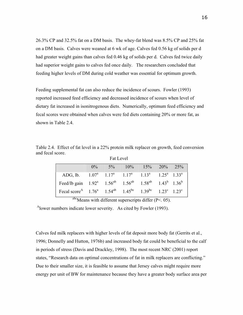
Feeding supplemental fat can also reduce the incidence of scours. Fowler (1993)
reported increased feed efficiency and decreased incidence of scours when level of
dietary fat increased in isonitrogenous diets. Numerically, optimum feed efficiency and
fecal scores were obtained when calves were fed diets containing 20% or more fat, as
shown in Table 2.4.
Table 2.4. Effect of fat level in a 22% protein milk replacer on growth, feed conversion and fecal score.
Fat Level
0% 5% 10% 15% 20% 25%
ADG, lb. 1.07a 1.17a 1.17a 1.13a 1.25a 1.33a
Feed/lb gain 1.92a 1.56ab 1.56ab 1.58ab 1.43b 1.36b
Fecal scoreA 1.76a 1.54ab 1.45bc 1.39bc 1.23c 1.23c abcMeans with different superscripts differ (P<. 05).
Alower numbers indicate lower severity. As cited by Fowler (1993).
Calves fed milk replacers with higher levels of fat deposit more body fat (Gerrits et al.,
1996; Donnelly and Hutton, 1976b) and increased body fat could be beneficial to the calf
in periods of stress (Davis and Drackley, 1998). The most recent NRC (2001) report
states, “Research data on optimal concentrations of fat in milk replacers are conflicting.”
Due to their smaller size, it is feasible to assume that Jersey calves might require more
energy per unit of BW for maintenance because they have a greater body surface area per
17 unit of BW, as indicated by their metabolic bodyweight, and thus are likely to use more
energy to maintain body temperature.
Protein requirements in the calf and the role of dietary protein
Protein is a critical component of the diet of the young calf. Amino acid requirements of
the calf are not well defined and are expressed in terms of nitrogen (Davis and Drackley,
1998). Level of CP in milk or MR, containing proteins derived from milk can be
calculated by multiplying the level of nitrogen (N) in the diet by 6.38 (NRC, 2001).
The Dairy NRC (2001) adopted the apparent digestible protein system (ADP) for
estimating the calf’s requirement for dietary protein developed by Roy (1970) and
calculated using the factorial method of Blaxter and Mitchell (1948).
ADP (g/d) = 6.25 [1/BV (E + G + M x D) – M x D]
where BV = the biological value of the protein;
E = endogenous urinary N;
G= N in gain;
M = fecal N;
and D = DM intake. (6)
The Dairy NRC (2001) sets BV at 80% for milk derived proteins, E is set at 0.2 g/kg of
metabolic BW, G is set at 30 g N/kg of LWG, M is set at 1.9 g/kg dm, and D is DM
intake in kg. The estimate of BV is based on the assumption that efficiency of N use for
growth above maintenance is 80% when the milk proteins are the source of N in the diet
(Donnelly and Hutton, 1976b). Estimates of urinary nitrogen and nitrogen in gain are in
agreement with values reported in the literature by (Blaxter and Wood, 1951; Roy, 1970).
Estimates of metabolic fecal nitrogen are based on the work of Roy (1980).
While components of the ADP equation (6) seem complex, the equation effectively
partitions dietary intake protein into maintenance or gain. This system of evaluating
protein requirements for the calf is more useful than the CP requirements recommended

18 by the 1989 Dairy NRC, which expresses the calf’s requirement for protein as CP but
does not attempt to estimate the portion of dietary protein that is utilized for maintenance
and gain. Developing a system for accurately estimating the requirement of amino acids
for calves would be an improvement over the ADP system. However, it is likely that the
calf’s requirement for amino acids is very similar to the amino acid profile in milk
proteins. Therefore, if the calf is fed a diet in which the protein sources are milk proteins,
milk proteins derivatives, or from other protein sources that have an amino acid profile
similar to milk then the ADP system is an adequate system for indirectly estimating the
amino acid requirements of the calf.
Dietary protein is essential for growth and development of a wide variety of tissues.
Several researchers (Diaz et al., 2001; Gerrits et al., 1996; Donnelly and Hutton, 1976b)
have demonstrated that level of dietary protein significantly impacts body composition.
Altering the ratio of protein to energy in the diet influences body composition of
preweaned calves. Davis and Drackley (1998) recommend that MR powder contain
between 18 and 24% CP. However, the appropriate level of CP in the diet depends on
the level of intake and energy supplied (Davis and Drackley, 1998). Calves consuming
high levels of DM (as a % of BW) or high-energy diets require more dietary protein for
lean tissue growth than calves on low energy or restricted levels of intake. This concept
is demonstrated in Table 2.5. At low levels of intake, a MR with 20% CP and 20% fat
supplies enough energy and protein to support similar rates of daily gain. At higher levels
of feeding, the energy supplied will support a greater rate of gain than the protein,
indicating that higher levels of protein in the milk replacer would improve rates of gain.
Therefore, it is important to balance or couple the calf’s protein and energy requirements.
Calves consuming milk or MR at or near ad lib intake require a higher level of protein
relative to energy than calves fed a restricted level of milk or MR.

19
Table 2.5. Energy and Protein allowable gains for a 22.7 kg calf fed a 20% fat, 20%
protein milk replacer at ambient temperature of 20°C .
DM fed Intake Allowable gain, kg %CP
kg % BW Energy ADP Required in MR
0.30 10 0.21 0.16 23.5
0.34 12 0.29 0.20 28.5
0.40 14 0.41 0.24 32.0
0.45 16 0.5 0.28 34.0
0.51 18 0.6 0.33 36.0
Values calculated using NRC (2001).
Development and history of milk replacers
Milk replacers were first manufactured in 1951. Development of MR occured primarily
for economic reasons; prior to 1951 calves were fed whole milk but the increasing market
value of milk created a market for lower cost ‘milk substitutes,’ i.e., milk replacers
(Fowler, 1993). Considerable research has been devoted to determining the most
nutritionally desirable and economical formulation for MR. Manufacturers of MR face
the constant challenge of providing a product to promote growth indistinguishable from
whole milk and yet be an economical alternative to whole milk.
Manufacturers of MR have considered digestibility of a wide variety of ingredients in
MR formulations. Butterfat, casein, and whey protein are the sources of fat and protein
in milk. These ingredients can be used in a MR formula; however, the cost of these
ingredients is generally too high to make a MR that is an economical alternative to whole
milk. Therefore, much research has been conducted on byproducts that can be used to
replace some or all of the butterfat, casein, and whey protein in milk replacer formulas.
Figure 2.1 outlines the process by which byproducts are derived from the processing of
milk. Nutrient composition of these byproducts is outlined in Table 2.6. These products
are often utilized in the formulation of MR because they are readily digestible and

20 economic alternatives to milk protein and yet have amino acid profiles that are similar to
milk protein.

21
Figure 2.1 . Steps in processing the associated byproducts used in manufacture of milk
replacers (Tomkins and Jaster, 1991) as cited by Davis and Drackely (1998).
Table 2.6. Chemical composition of milk byproducts (% of DM). Ingredient Dry Matter Crude Protein Crude Fat Lactose AshDried skim milk 98 34 0.1 54 5.6Whey protein concentrate 98 34 3.5 52 6.0Dried whey 98 12 0.2 74 8.5Delactosed whey 98 23 1.5 55 16.0Sodium caseinate 96 85 0.5 - 2.5 Adapted from (Davis and Drackley, 1998)
Non-milk sources of protein considered in the formulation of milk replacers include
wheat protein, potato protein concentrate, soy protein concentrate, soy flour, meat

22 solubles, fish protein concentrate, sprayed dried red blood cells, and animal plasma.
However, digestibilities of these alternative protein sources are inferior to skim milk
(Table 2.7). Reasons for inferior digestibility of non-milk protein sources are largely due
to differences in the amino acid profile of these proteins. Many of these proteins have
anti-nutritional factors. Soy proteins contain protease inhibitors that interfere with the
ability of digestive enzymes including trypsin and chymotrypsin to digest proteins. In
addition, soy proteins contain antigenic proteins that result in allergic reactions in young
calves (Davis and Drackley, 1998). Other proteins, for example wheat proteins, have
lower digestibilities in the young calf but improved digestibility in older calves (Davis
and Drackley, 1998). More recently, proteins from blood sources, e.g. plasma and red
blood cells, have been consider for use in MR. Quigley et al. (2000) evaluated red blood
cell protein in MR and was able to replace up to 43% of the protein in the MR without
affecting weight gain, feed efficiency, starter intake, fecal scores or d scouring, indicating
that the red blood cell protein could be an alternative source of protein for use in MR.
Table 2.7. Crude protein digestibility of milk replacers containing various protein
sources.
Percent of milk CP digestibilityProtein source protein replaced %
Skim milk - 97.0Whey protein concentrate 100 90.2Whey proteins 100 89.9Soluble wheat protein 20 94.9Modified soy flour 50 72.1Heated soy flour 50 64.1Soy protein concentrate 75 58.7Soy flour 75 54.8Meat solubles 33 54.8Fish flour 67 83.7Fish protein concentrate 100 53.8
Adapted from (Davis and Drackley, 1998).

23 Butterfat is highly digestible but is also very expensive. However, other saturated fats
including tallow, choice white grease, and lard are very digestible and acceptable for use
in MR formulation. Unsaturated fats such as, most vegetable oils, are generally
unsatisfactory in MR because they have lower digestiblities and cause diarrhea in calves
(Jenkins et al., 1985). However, coconut and palm oils may be used in combination with
animal fats in MR, these oils are more digestible (92-96%) than most vegetable oils
(Toullec et al., 1980).
Intensified rearing of calves
Liquid feeding schemes have been suggested to promote rapid growth of calves. Calves
fed conventional liquid feeding schemes, i.e. 8 to 10% of BW, gain little during the first
weeks of life, later increasing to rates rarely exceeding 250 to 400 g/d. Mowrey (2001)
fed Jersey and Holstein calves MR (20% fat and 20% CP) reconstituted to 12.5% solids
at a rate of 31% of metabolic BW. Sufficient energy was provided for 227 g ADG
according to NRC (2001). Figure 2.2, demonstrates the lack of BW gain during the 1st
two weeks of life and indicates that feeding calves a 20/20 MR at 31% of metabolic
weight provides only enough energy to maintain BW. Jersey calves showed little or no
increase in BW from birth to 22 d. However, BW began to increase in Holstein calves
after d 15. The diets were designed to support 227 g of ADG and calves should have
gained more than 8 kg BW over the duration of the experiment but the Jersey calves
gained less than 5 kg BW. This indicates maintenance energy requirement of Jersey
calves may have been higher per unit of metabolic BW than Holstein calves and that
NRC (2001) equations for maintenance energy may not be appropriate for Jersey calves.
Increasing the feeding rate and/or increasing the caloric content of the liquid diet may
improve the growth of young calves and this maybe particularly important in Jersey
calves.
Feeding schemes designed to promote higher ADG and feed efficiency by allowing
calves to consume more MR than 8 to 10% of BW are referred to as ‘intensified’ feeding
schemes. Generally, these schemes are designed to provide enough nutrients in the liquid

24 diet to support ADG of 1000 g or more in Holstein calves (Drackley, 2001). Intensified
feeding programs promote rapid growth and are associated with improvements in feed
efficiency because as the level of DMI increases, a smaller fraction of the DM consumed
is required for maintenance and more energy is available to support growth. The feed
efficiency of lambs and piglets is generally much higher than that of calves because these
animals consume more DM per unit of metabolic BW (Figure 2.3). A calf fed liquid
feed at 8 to 10% BW consumes approximately 2.7 units of feed DM per unit of gain but
lambs and piglets allowed ad lib intake of milk often achieve feed efficiencies of less
than 1.5 units of feed per unit of gain. Theoretically, calves can gain at similar levels of
feed efficiency when fed similar levels of DM per unit of metabolic BW.
20
25
30
35
40
45
50
55
0 8 15 22 29Time (d)
Bod
y W
eigh
t (kg
)
Significant cubic effect (P < .01)Significant quadradtic effect (P < .01)Significannt linear effect (P < .01)
SE ~ 1.47
Figure 2.2. BW (kg) on d 1 to d 29 of Holstein females (♦), Holstein males ( ), Jersey
females ( ), and Jersey males (×). Significant breed by time interaction; differences
detected on all d. (Mowrey, 2001).

25
Figure 2.3. Efficiency of feed conversion. Adapted from (Davis and Drackley, 1998).
Increased weight gain has resulted from feeding MR with increased nutrient density or
increasing the amount of DM fed each d. Khouri and Pickering (1968) fed calves
reconstituted whole milk at 11.3, 13.9, 15.9 and 19.4% of BW. Average BW gain
increased from 410 to 940 g/d and feed efficiency increased, particularly between the two
intermediate levels of intake.
Bartlett (2001) varied both rate of feeding and level of CP in diets fed to Holstein calves
in a series of experiments. In one experiment, MR (reconstituted to 12.5% DM) was fed
at 10% or 14% of BW and CP in the MR varied from 14% to 26%. In another
experiment, calves were fed milk at either 8.32% or 11.65% of BW or MR with similar
nutrient density to milk at 11.65% of BW. The results are reported in Table 2.8.
Increasing rate of feeding resulted in increased feed efficiency and an increase in body fat
%. Increasing level of CP in the diet also increased the level of feed efficiency but
0.61
1.41.82.22.6
33.43.84.24.6
10 30 50 70 90
Dry Matter Intake
Feed
con
vers
ion
(kg
feed
/kg
gain
)
(g/kg BW.75)
CalfLamb
Piglet

26 decreased body fat %. Calves fed milk and a MR with similar nutrient density to milk had
similar feed efficiencies and body fat %.
There appears to be a significant role of dietary protein in the intensified calf feeding
schemes. Tomkins and Sowinski (1995) fed calves isocaloric diets with varying levels of
CP. Average daily gain increased as dietary protein increased with the highest ADG
from birth to 42 d in calves fed a MR containing 24% CP and 18.5% fat (Table 2.9).
The g of ADP required to support a target rate of gain for a calf of a given BW can be
determined using equation (6), and then ADP can be converted to CP based on the
digestibility of the protein source in the diet. Finally, the CP concentration required in
the MR can be determined by dividing the g of CP required by the estimated DMI of the
calf. Some examples of CP levels for a calf weighing 22.7 kg are shown in Table 2.5.
(Davis and Drackley, 1998) calculated that a calf weighing 45.4 kg and gaining 1134 g/d
requires a MR that contains 27.2% CP. Therefore, the theoretical level of CP in a MR
designed for intensified feeding programs is somewhere between 27% and 30% CP.

27 Table 2.8. The effect of varying the level of intake and crude protein on feed efficiency
and body fat deposition.
Feeding Rate CP Fat Feed efficiency Fat% of bw % of DM % of DM gain/unit of feed % in body
10.0 14.0 22.0 0.40 6.810.0 18.0 20.7 0.48 5.910.0 22.0 19.4 0.55 5.610.0 26.0 18.1 0.61 5.114.0 14.0 22.0 0.52 8.814.0 18.0 20.7 0.59 8.114.0 22.0 19.4 0.72 7.114.0 26.0 18.1 0.71 6.6
8.32m 25.4 27.1 0.49 5.4 11.65m 25.4 27.1 0.72 6.711.65 26.0 28.0 0.65 4.1
mWhole milk.
(Bartlett., 2001)
Table 2.9. The influence of protein levels in milk replacers on growth and performance.
of Holstein male calves fed isocaloric diets to 42 days of age.
Treatment 1 2 3 4 5 6 MR
fed g/d Crude protein% 14 16 18 20 22 24 Crude fat % 22.0 21.3 20.6 20.0 19.2 18.5
ADG g
D 1-7 -45a 45ab 91b 64b 104b 18ab 454
D 8-14 32a 77a 109ab 86ab 91ab 163b 567
D 15-21 449a 485a 499ab 481a 567bc 603bc 680
D 1-42 322a 376b 386b 404bc 422bc 440d 737 abcdMeans with different subscripts differ (P<0.05).
(Tomkins and Sowinski, 1995) as cited by Davis and Drackley (1998).
Gerrits et al. (1996) conducted two experiments using Holstein Friesian x Dutch Friesian
calves by varying the ratio of protein to energy (g digestible protein/MJ protein free
energy) from 8.5 to 20.0 and from 6.0 to 18.5 in experiments one and two, respectively.

28 Calves in experiment one were reared from 80 kg to 160 kg and were fed either 663 or
851 kJ of protein-free energy per kg of metabolic BW. In experiment two, calves were
fed either 564 or 752 kJ of protein-free energy per kg of metabolic BW. Protein
digestibility increased as intake of protein increased in both experiments. Increased
protein intake resulted in an increased deposition of both protein and fat. Daily intakes of
244 g of protein resulted in maximum protein deposition. However, as the level of
dietary protein increased, only 30% of the extra protein in the diet was deposited as tissue
protein.
Donnelly and Hutton (1976a, 1976b) fed Friesian bull calves MR that ranged from 15.7
to 29.6% CP. Calves were fed for target ADG of 610 or 830 g. Body composition was
altered as level of protein in the diet changed. Calves fed a MR containing 29.6% CP had
the greatest digesta-free body protein % and the lowest proportion of energy gain as fat.
Conversely, calves fed a MR containing 15.7% CP had the lowest digesta-free body
protein % , highest % body fat, and the highest proportion of gain as fat (Table 2.10).
Calves fed diets containing higher levels of protein had a reduction in body fat and an
increase in digesta-free body protein.
In a similar experiment, Diaz et al. (1998) adjusted intake of a MR in an attempt to
achieve target ADG of 500 g, 950 g, or 1400 g. A 30% CP MR was selected so that
protein would not limit growth. Feed efficiency (gain/feed) increased from 0.64 to 0.74
between the extremes of the diets. Calves fed for a target gain of 1400g/d per d
deposited more body fat and less protein than the calves fed for 500g ADG.

29
Table 2.10. Content of the gross chemical components and energy in digesta free body
weight gains.
Dietary crude protein (%) 15.7 18.1 21.8 25.4 29.6 31.5
Component
Water (%) 58.9 59.9 61.7 62.3 62.8 64.5
Fat (%) 22.3 20.0 18.4 15.3 11.7 11.8
Protein (%) 16.6 17.2 17.3 19.0 21.5 19.6
Ash (%) 2.3 2.6 2.7 3.3 3.8 4.1
Energy (MJ/kg) 12.4 11.9 11.2 10.7 9.5 9.3
Proportion of energy gain as fat 0.70 0.66 0.64 0.58 0.47 0.51 From Donnelly and Hutton (1976b).
The research clearly demonstrated that calves fed intensified feeding programs require
higher levels of CP for lean growth (Bartlett, 2001; Gerrits et al., 1996; Donnelly and
Hutton, 1976a; Donnelly and Hutton, 1976b; Diaz et al., 2001). Increasing the rate of
feeding of MR increases ADG and feed efficiency regardless of the level of CP in the diet
but feeding low CP MR results in a composition of gain that has more fat and less protein
than higher CP MR.
Rapid growth and heifer development
Few research trials have examined long-term effects of accelerated growth in the
preweaned calf on mammary development and milk production. Previous work (Sejrsen
et al., 1982; Swanson, 1954; Swanson, 1960; Capuco et al., 2000) demonstrated that
rapid growth (ADG >1 kg) in heifers between 3 mo of age and puberty can be detrimental
to mammary development and future milk production. At least three theories exist for
the negative relationship between rapid growth and mammary development. The first
theory involves growth and development of the mammary gland. The mammary gland
grows more rapidly than the animal from approximately 3 mo of age to puberty. Heifers

30 that grow rapidly during this period of time deposit a disproportionately high amount of
fat in the mammary gland. Swanson, (1960) proposed that deposition of fat in the
mammary gland led to reduced milk production in the mature animal. The second theory
is an endocrine theory; rapid weight gains in prepubertal heifers result in shifts in
hormonal concentrations. Sejrsen et al., (1983) suggested that shifts in growth hormone
or other hormones in heifers that were growing rapidly during the prepubertal period
resulted in a reduction in parenchymal tissue development. More recently, a third theory
has been proposed by VandeHaar and Silva, (2002). The new theory suggests that
adipose tissue in the mammary gland may secrete compounds and/or hormones that
interfere with the synthesis of parenchymal tissue. However, not all experiments have
shown a negative relationship between rapid rates of growth during the prepubertal
period and future milk yield (Sejrsen, 1997) indicating that the relationship between
growth and mammary gland development is very complex.
Few studies have examined the influence of gains in the preweaned calf on body
composition and mammary development. In one such study, Sejrsen et al. (1998) fed
preweaned calves MR with 58 g or 73 g CP/Mcal ME from 5 to 42 d of age and
demonstrated that rate of gain in the preweaned calf did not affect mammary tissue
development. Diets resulted in ADG ranging from 632 to 895 g from d 5 to 42. Calves
were sacrificed when their BW reached 250 kg. There was no difference in amount of
parenchymal tissue between treatments indicating that rapid growth from 5 to 42 d of age
was not detrimental to mammary development.
Rapid growth and future milk yield
Assessing, parenchymal tissue development provides an indirect estimate of future milk
yield. However, conventional methods of measuring parenchymal tissue involves
removal of the mammary gland thus preventing lactation. Few studies have examined the
relationship between pre-weaning diet and future milk yield in young calves. Bar-Peled
et al. (1997) fed Holstein calves either MR (control) or allowed calves to suckle their
dams for 15 min twice per d. Control calves consumed 3.33 L of MR (3.0% fat and 4.6%

31 CP, as fed) per day, while intake of suckled calves averaged 16.9 kg/d of milk (3.12% fat
and 3.28% CP). Calves that were suckled had gained nearly 300 g more per d from birth
to 6 wk of age. They were 30 d younger when they conceived, 5.3 cm taller and 37 kg
heavier at calving, and produced 453 kg (P<0.08) more milk in their first lactation. In a
similar experiment, Danish researchers (Foldager et al., 1997) fed Danish Black and
White calves from 5 to 42 d of age 4.6 kg/d of whole milk or allowed calves to consume
milk ad libitum from their dams or from an open bucket. Ad libitum intake of milk
increased ADG by approximately 200 g/d from birth to 42 d of age. Calves that
consumed milk ad lib produced 1.6 kg more milk/d in their first lactation, gained 16.4 kg
more BW in the first 250 d of lactation, and tended to consume more dm (0.6 kg/d)
during their first lactation. No difference was detected in milk production between calves
that suckled or consumed milk ad libitum, indicating that level of milk intake and not
presence of the dam resulted in higher levels of production.
Body composition analysis
Growth can be measured as an increase in BW or an increase in frame size. However,
these measures ignore composition of gain. It is likely that there is an optimum
composition of gain in calves. Diet and rate of gain have an influence on composition of
gain. Several researchers suggest that maximizing protein content of gain is optimum in
the young calf (Diaz et al., 2001; Davis and Drackley, 1998; Gerrits et al., 1996;
Donnelly and Hutton, 1976b). However, few if any long-term studies have been
conducted relating composition of gain in young calves to future milk production and
performance.
Whole body analysis of composition
Body composition of animals has been of interest to scientists for well over 100 years.
(Reid et al., 1955) reviewed the history of body composition analysis in farm animals and
noted that in the late 1800’s, German researchers including von Berzold, (1881), von
Hosslin (1881), and Pfeiffer, (1886) published results of studies that evaluated the
composition of animals. German researchers developed a methodology for evaluating
body composition and studied mammals, birds, amphibians, and fish. These researchers
32 found that morphologically similar animals had similar body compositions.
Methodology of determining composition has been refined since these early experiments.
Powell and Huffman (1968) reported that the most accurate method of assessing carcass
composition required animal sacrifice and chemical analysis. Contemporary researchers
(Diaz et al., 2001; Bartlett, 2001; Tikofsky et al., 2001; Donnelly and Hutton, 1976b;
Gerrits et al., 1996) have analyzed body composition of calves by sacrificing the animal
and conducting chemical analysis of the body. The methodology varies between
researchers but the general principal involves sacrifice and dividing the animal into three
or four components. These components are then homogenized in a grinder and sub-
sampled to permit analysis to determine their composition and a weighted average is
calculated to estimate empty body composition of the animal.
Multi-compartment models of analysis
Composition of an animal can be broken down into many different levels including the
atomic, molecular, cellular, and tissue (Heymsfield and Wang, 1997). At the atomic level,
the composition of the animal can be described in terms of the elements that make up the
animal. At the molecular level, the body can be broken down into lipids, water, proteins,
carbohydrates, and minerals (Wang et al., 2002). At the cellular level, body composition
can be described in terms of cell mass, extracellular fluid, and extracellular solids.
Theoretically, body composition could be measured on the sub-atomic level, however,
the usefulness and practicality of measuring composition at the sub-atomic level is
questionable. Measuring body composition at the tissue level is generally the most
useful in humans and animals as body fat % and bone mineral density are frequently
associated with performance, disease, and health. At the tissue level, the body can be
described as adipose tissue, visceral tissues, skeletal muscle, bone, and brain (Heymsfield
and Wang, 1997).

33 In cattle, the most common model of body composition is the molecular model of body
composition because researchers are most interested in determining the level of fat,
protein, and ash in the body. In beef cattle, deposition of body fat in the tissue is related
to market value, and analyzing the body composition of the live animal provides an
assessment of market value of the animal. The molecular model of body composition is a
multi-component model of body composition with five to six components: fat, water,
protein, glycogen, bone mineral, and non-bone mineral. This model is often modified
into simpler models with fewer components (Figure 2.4). The five component (5-C)
model of body composition is often reduced into two component (2-C) models of body
composition such as fat and fat free components, or bone mineral and soft tissue (Buzzell
and Pintauro, 2001). In many cases, only a few of the five components of body
composition are of interest and the reduced models are more practical than the 5-C
model.
Figure 2.4. Models of body composition. On the left is a two component (2-C) model of body composition showing fat and fat free mass. On the right is a six component (6-C) model of body composition showing fat, water, protein, glycogen, non-bone mineral, and bone mineral. Courtesy of Buzzel and Pintauro (2001).

34
Common methods of analyzing body composition
Methods of analyzing body composition can be divided into two broad categories.
Invasive methods of measuring body composition involve subjecting the animal to
procedures that cause some degree of pain and/or discomfort for the animal, and in some
cases may interfere with organ function. The most invasive methods of analysis require
sacrificing the animal. Non-invasive methods of analysis cause little pain or discomfort
to the animal, but in many cases, these methods provide estimates of composition that are
less reliable than invasive measures of composition.
Dilution
Dilution techniques have been used to evaluate body composition of animals in vivo.
Dilution techniques utilize the relationship between body water and other components. A
reduction in water content accompanies an increase in body fat (Moulton, 1923; Powell
and Huffman, 1968). As percentage fat in an animal increases, the concentration of
water, protein, and ash in the empty body are diluted (Moulton, 1923). Body fat
percentage can be estimated indirectly from measurements of body water in an animal.
Urea space (US) is one such technique. Bartle et al. (1987) used the following technique
to determine US in Hereford x Angus and Chiania steers. Blood samples were drawn
before and 12 min following infusion of a saline solution (0.66 ml/kg live weight)
containing 20% urea. Then US was estimated using the following equation
US = mg urea-infused/(change in PUN x Live weight x 10)
where PUN was expressed as mg urea-N/100ml (7)
Steers were then slaughtered and the right half of the carcass and all of the internal
components were analyzed to determine fat, nitrogen, and water content of the empty
body (EB). The cattle ranged between 6.5 and 38% body fat. Equations were developed
to predict water %, fat %, and nitrogen % in EB based on US and live weight. These
equations were correlated to chemical composition (r2 =0.67). Hammond et al. (1990)

35 evaluated US with Holstein steers and developed equations to predict empty body fat,
protein, and water that were correlated to chemical analysis (r2 = 0.95, 0.95, 0.83,
respectively). Hammond et al., (1988) suggested that repeated measurements of US
throughout a feeding trial provided a better estimate of body composition than a single
measurement due to inconsistency in estimates of US. Dilution techniques provide
reasonable estimates of EB composition in animals that are chemically mature. In cattle,
body water content decreases in fat-free mass from conception until chemical maturity at
5-10 months of age. Chemically maturity can by defined as the point in time when the
animal’s body water remains relatively constant; cattle remain ‘immature’ to
approximately 200 d of age and from 200 to 500 d of age, they are in a transition until
chemical maturity is reached at approximately 500 d of age (Reid et al., 1955).
Estimates of body composition based on US in young animals that are not yet chemically
mature may be inaccurate.
Bioelectrical impedance
Bioelectrical impedance analysis (BIA) is frequently used to evaluate body composition
in human subjects. This technique is based on the ability of tissues to conduct an
electrical current. Aqueous tissues conduct electricity due to dissolved electrolytes.
Impedance is the resistance of a biological conductor to the flow of alternating current
(Brodie et al., 1998). Impedance of tissue is affected by the volume of the conductor
(i.e., the volume of the subject), length of the conductor (i.e., the height of the subject),
and presence of dissolved electrolytes. Adipose tissue and bone mineral are poor
conductors i.e., have a high degree of impedance. On the other hand, soft lean tissues are
good conductors of electricity due to the presence of dissolved electrolytes. Differences
in electrical conductivity in bone mineral, adipose tissue, and lean soft tissue can be used
to estimate body composition (Ellis, 2000). Zack (2002) evaluated body composition of
human subjects (average age 22.7 yr) with both BIA and dual energy x-ray
absorptiometry (DXA) and reported a high correlation between BIA and DXA (r= 0.998)
for estimates of body fat %, lean body mass, and fat mass, indicating that BIA is an
appropriate method of evaluating the body composition of human subjects.

36
Human subjects are frequently evaluated with BIA because it is safe, measures body
composition rapidly, noninvasive, inexpensive, portable. However, the theory behind
BIA assumes an object is a perfect cylinder with uniform cross-sectional area. Humans
and animals do not fit this description, and inaccuracy in estimation of body composition
is likely to result (Zack, 2002). Factors other than body composition can affect
conductivity of a human subject including differences in gender, age, ingestion of a meal
prior to measurement, muscle mass, physical activity, menstrual cycle, degree of
hydration, and position of electrodes (Brodie et al., 1998). It is unlikely that BIA is
appropriate for assessing body composition in calves because of these variables. In
particular, the level of hydration or dehydration in a calf is an area of concern. Diarrhea
is common in calves and results in varying degrees of dehydration and electrolyte
balance.
Another method that is frequently used to evaluate body composition in humans is
underwater weighing (UWW). This is a 2-C model of body composition (fat and lean
tissue) and is often considered the gold standard for evaluating body composition in
humans. Lean tissue is denser than fat, thus the density of a human can be used to
estimate their body composition (Ellis, 2000). Archimedes principle states that an object
will displace a volume of water equal to its volume when submersed in water; UWW
utilizes this principal to determine the density of the body (Buzzell and Pintauro, 2001).
Body composition is determined by comparing the volume of water displaced and/or the
subject’s weight, when they are submersed in a tank of water, to their BW. A few
technical adjustments must be made to account for the air volume of the lungs because
the presence of air in the lungs will alter the volume of water displaced by an individual.
Ellis (2000) reported that every 100-ml error in estimation of lung volume results in an
increased uncertainty of measurement of body fat of ~1%. In humans, lung volume is
determined and accounted for in the equations used to estimate body fat. Determining
lung volume in animals is difficult. However, this method has been used to evaluate the
body fat in animal carcasses. In one such study, (Elowsson et al., 1998) reported a
37 correlation of (r = 0.77) between UWW and chemical analysis in estimation of body fat
mass in pig carcasses.
Dual x-ray absorptiometry analysis of body composition
Dual-Energy X-ray absorptiometry (DXA) was first introduced in 1987 for use in
evaluating bone mineral density in human subjects (Zack, 2002). Recent estimates by
the National Osteoporosis Foundation indicate that 89% of bone mineral density tests
performed in the United States utilize DXA (Smith and Shoukri, 2000). This technology
has gained widespread acceptance because of its accuracy, precision, fast scanning time,
and non-invasive nature (Heymsfield et al., 1989; Ellis, 2000; Hansen et al., 1990; Zack,
2002). There are three manufacturers of DXA equipment: Hologic, Lunar, and
Nordland. The basic components of the DXA instrument manufactured by Hologic are
an X-ray generator and tube that produces a fan shaped beam at 2 energies, 100 kVp and
140 kVp, and a cadmium tungstate detector (Zack, 2002). A computer and software
package also are required for interpreting the readings detected by the DXA instrument.
Available software packages available allow the estimation of bone mineral density and
body composition.
Body composition is estimated by DXA utilizing a three-component model of body
composition (i.e., fat, lean, and bone mineral mass). Ellis (2000) explained the principle
of DXA in the following way, “When an x-ray or photon source is placed on one side of
an object, the intensity of the beam on the opposite side of the object is related to its
thickness, density, and chemical composition.” The difference between the initial
intensity and the final intensity of the x-ray that was passed through an absorber (e.g.,
tissue) is called attenuation. The ratio of attenuation in the high energy and low energy
beam are referred to as an attenuation ratio (Rst) in soft tissue. Svendsen et al. (1993)
reported that Rst and fat % are inversely and linearly related, which allows fat % in soft
tissue to be calculated based on its Rst. Using the Rst, DXA can distinguish between

38 adipose tissue and lean tissue; this is a 2-C model of body composition. In a similar
manner, DXA is also capable of distinguishing between bone mineral tissue and soft
tissue, which is another 2-C model of body composition. Therefore, DXA
simultaneously measures two 2-C models of body composition. Bone mineral does not
contain any fat; therefore, when DXA has distinguished between the bone mineral and
the soft tissue, then the estimates of fat and lean tissue can be applied to the soft tissue.
The result is a 3-C model of body composition that yields bone mineral mass, fat mass,
and lean tissue (excluding bone mineral) mass.
In addition, DXA has also been utilized to evaluate body composition of pigs (Elowsson
et al., 1998; Mitchell et al., 1998a; Mitchell et al., 1998b; Mitchell et al., 1996) and
chickens (Mitchell et al., 1997). In early studies, pigs were used to evaluate and
calibrate DXA for measuring body composition in human infants and small children
(Ellis, 2000). More recently, DXA has been evaluated as a method of measuring body
composition in live pigs to provide information on body composition that could be useful
in determining market value of the carcass in the live animal.
In a study with eight,12-wk old Swedish Landrace x Yorkshire piglets (15-22 kg),
Elowsson et al. (1998) compared DXA, underwater weighing (UWW), and chemical
analysis as measures of body composition. Pigs were euthanized, and head, thoracic
organs, abdominal organs were removed. Each carcass was scanned three times with
DXA (DPX-L, Lunar, Madison, WI) and body composition was estimated using a
pediatric software package (Pediatric, 1.5b, DPX-L, Lunar). Following DXA analysis
carcasses were analyzed using UWW. The carcasses were weighed first in air and then in
water. Carcass density was calculated as:
CD = [(weight in air)/(weight in air – weight water)]/density of water (7)
Fat free mass was calculated as:
% fat = (a/CD – b) x 100; where a and b are constants for density of fat and fat
free mass, respectively. (8)

39 Finally, the carcasses were divided along the midline and the right half was dissected into
forelimb, hind limb, and remainder of the carcass was separated into muscle, fat, and
bone. These components were homogenized and analyzed for fat and bone mineral.
Chemical analysis of body composition was taken as the most accurate measure of
composition and DXA estimates and UWW were compared with values derived using
chemical analysis. Correlations between DXA and chemical analysis for body
composition were highly correlated (r = 0.90 – 1.0). However, DXA overestimated bone
mineral mass, lean mass, total weight, and underestimated fat mass. Even so, DXA was
a better predictor of fat mass than UWW (r = 0.77), which also overestimated fat mass.
In studies using similar methodology as Elowsson et al. (1998), Mitchell et al (1998b)
examined composition of pigs. They reported a high correlation (R2 = 0.97) between
DXA measurement of lean tissue mass (total mass – fat and bone mass) and carcass
protein in pigs weighing 10 to 61 kg (Mitchell et al., 1998b). In a study with small pigs
(5-27 kg), Mitchell et al. (1998a) developed an equation that regresses DXA on carcass
protein. The resulting equation accurately predicted carcass protein (R2 = 0.92). In the
same study, DXA estimated bone mineral content within 2% of estimates of BMC from
total body ash.
The usefulness of DXA has been evaluated in estimating whole body composition of pigs
and DXA may be useful for evaluating body composition of calves. Generally, invasive
methods of body composition analysis are applied to calves requiring sacrifice of the
animal. These methods do not allow body composition in individual animals to be
measured at different points in growth and development. Nor do current methods of
body composition analysis in calves allow for body composition of individual animals to
be related to future performance. Researchers have reported a relationship between the
rate of growth in young calves and future milk performance including milk yield (Bar-
Peled et al., 1997; Foldager et al., 1997). Changes in body composition of young calves
due to diet may explain the differences in future performance, but the invasive measure
of body composition that are commonly used to evaluate calves make it difficult to test

40 this hypothesis. Non-invasive measures of body composition like DXA would be useful
in testing this hypothesis.
What is the ideal body composition?
Considerable time and effort have been devoted in this treatise and others to consider
alterations in body composition and methods of determining body composition of calves.
However, a question that begs to be asked is, “What is the ideal body composition of a
dairy replacement heifer?” As stated previously, the literature indicates that in the
prepubertal heifer (>3 mo. of age to puberty), growth rates in excess of 1 kg/d result in
reduced first lactation milk yield (Swanson, 1960). However, few if any studies relating
growth rate of prepubertal dairy heifers and future milk yield have evaluated body
composition of these animals. Therefore, the relationship between body composition
and future milk yield in prepubertal heifers is difficult to elucidate. Limited research has
been conducted that assesses the relationship between growth and body composition of
young calves and future milk yield. As stated previously, (Sejrsen et al., 1998) reported a
positive relationship between growth and mammary and parenchymal development when
calves were fed for rapid gains from birth to 6 wk of age but a negative relationship after
six weeks of age. In a similar study, Foldager et al. (1997) reported ad lib feeding from
birth to 6 wk of age improved first lactation milk yield by 1.6 kg/d compared to
conventional feeding (MR fed at 10% of BW). Ad lib feeding from birth to 12 wk of age
resulted in a 3.6 kg/d reduction in milk yield compared with conventional feeding.
Theoretically, calves fed ad lib deposit more adipose tissue and have a higher percentage
body fat than calves that are limit-fed. Even though body composition was not measured
by Foldager et al. (1997), or Bar-Peled et al. (1997), it is reasonable to conclude that the
calves fed ad lib diets had higher levels of body fat than calves fed the control diets. If
this is true, then it would appear to be advantageous to feed calves from birth to 6 wk for
rapid growth and deposition of fat. Results of Sejrsen et al. (1998) and Foldager et al.
(1997), would indicate that deposition of body fat from 6 to12 wk of age is detrimental to
future milk production. These hypotheses should be tested directly.

41 The relationship between body composition and future performance has been measured
in other species. Several such studies have been conducted with poultry. Yannakopoulos
et al., (1995) reported that increased carcass fat in Japanese quail resulted in an earlier
age at first lay and determined age at onset of sexual maturity. Similar results have been
reported with broilers (Robbins et al., 1988) dwarf and normal chickens (Brody et al.,
1984), and white turkey hens (Renema et al., 1994). Zelenka et al., (1984) found that
body composition affected early maturing and late maturing quail differently. In the
early maturing quail the first lay was a function of chronological age and % body lipid,
but in late maturing quail a critical lean weight and/or skeletal development determine
sexual maturity. Renema et al., (1994) fed male line large white turkey hens from wk 4
to 28 either full feed or diets that were restricted so that BW was either 10 or 20% less
than full fed controls. The birds fed for a 20% reduction in weight had less breast muscle
and abdominal fat early in lay, and sexual maturity was delayed, but the birds fed
restricted diets had an increase in settable egg production. Therefore, diet restriction is
desirable in breeder hens even though sexual maturity is delayed. Moran et al., (1983)
also found that decreased fat accretion early in sexual maturity improved reproductive
capacity apart from an alteration of BW in small white breeder toms. In poultry nutrition,
restricting the diet and reducing fat accretion may improve reproductive performance in
breeders. However, age at sexual maturity and/or age at first lay is reduced by increasing
body fat deposition. It is important to note that poultry differ from other species of
production. Poultry have been genetically selected for very rapid rates of gain and rapid
deposition of body fat. Broilers are capable of reaching market weight by 7 wk of age
(Cheeke, 1999). However, rapid rate of gain does not favor reproduction and the ability
of broilers to gain weight and deposit fat can result in leg problems and reduced egg
production. Thus, broiler breeders are typically fed diets that restrict levels of energy to
slow rate of growth and improve reproduction. Poultry are very different than cattle and
other mammals physiologically, and chicks have a very different diet than neonatal
mammals.

42 In mammals, sexual maturity and body composition do not appear to be as closely related
as in poultry. Rozeboom et al. (1995) reported that age at puberty is not related to body
composition in gilts. The relationship between body composition and sexual maturity has
been considered in cattle. The plane of nutrition, particularly level of energy in the diet,
is inversely related to age at puberty in cattle (Greer et al., 1983; Buskirk et al., 1995;
(Maas, 1987). Simpson et al. (1998) tested the hypothesis that a critical body fat % must
be reached in cattle to initiate puberty; they reported body fat % didn’t significantly affect
variation in age at first conception in beef heifers but a combination of BW, body
condition score, BW gain, and age may initiate the onset of puberty in heifers. The
results of Simpson et al. (1998) led to the conclusion that body composition alone
doesn’t determine the onset of puberty.
The ‘ideal’ body composition of a dairy replacement heifer in terms of future
composition is not known. Some researchers (Van Amburgh, 2002; Drackley, 2001)
suggest that the goal of calf rearing is to maximize the rate of lean tissue growth. On the
other hand the work of Swanson (1954, 1960, 1967), Serjsen et al. (1982), Sejrsen et al.,
(1983) Sejrsen et al., (1998), Sejrsen et al., (2000), Sejrsen, (1997), and several others
using older prepubertal heifers would lead us to believe that slower rates of gains might
favor lifetime performance.
Objectives
Recent studies have indicated a possible relationship between calf feeding programs and
growth and development of the heifer after weaning. Ratios of energy to protein in MR
influence composition of BW gain
Therefore, the objectives of this study are to examine the relationship between dietary
protein and energy on ADG, empty body weight gain, wither height, heart girth, body
length, hip height, body composition, protein retention, efficiency of energy utilization,
feed efficiency, and health in Jersey bull calves. We will also compare dual energy X-ray
absorptiometry estimates of body composition to chemical measures.

43
Chapter Three
Calf Mortality Surveys
Introduction
Calf mortality has a significant economic impact on the dairy industry. In recent years,
the price of replacement dairy heifers has increased, indicating that heifers are in short
supply. The USDA sponsored the National Dairy Heifer Evaluation Project (NDHEP) as
a part of the National Animal Health Monitoring System (NAHMS). The NAHMS
reported a mean death loss between birth and weaning of 8.4 and 11.4% in 1993 and
1996, respectively. The increase in calf mortality between 1993 and 1996 indicates that
supply of dairy heifers may be declining due to an increase in calf mortality.
The purpose of NDHEP was to collect information on health and management
characteristics that could be related to the long-term health and economic performance of
heifers (Losinger and Heinrichs, 1997). Data were collected from 1685 dairy operations
during 1991 and 1992. Participating herds were representative of 78% of the dairy herds
in the United States (Heinrichs et al., 1994). These herds reported 47,057 births and 4427
deaths (9.4%) in preweaned calves (Losinger and Heinrichs, 1997). Average herd size
was 86 mature cows and 66 heifers (Losinger and Heinrichs, 1997). However, the
majority of herds, 94.9%, were Holstein herds, and only 2.4% of herds surveyed were
Jersey herds (Heinrichs et al., 1994).
Calf mortality as reported by NDHEP (NAHMS, 1993) is broken down by cause in Table
3.1. Several studies have shown that calf mortality is related to a variety of management
factors and/or factors that are indicative of the level of herd management. Table 3.2 lists
major risk factors associated with calf mortality. Health, management, and feeding
practices associated with calf mortality will be discussed in detail in the following
sections of this treatise.

44
Table 3.1. Causes of death in preweaned calves
Cause of death % Death loss SE
Scours, diarrhea 4.4 ±0.4
Respiratory problems 1.8 ±0.1
Joint or navel problems 0.2 ±0.1
Trauma 0.2 ±0.1
Other 1.0 ±0.2
Unknown 0.8 ±0.1
(Heinrichs et al., 1994; NAHMS, 1993)
Table 3.2. Factors associated with mortality in preweaned calves as determined by
several regional and national surveys.
Risk Factor Relationship
Region of the country Higher mortality in western herds
Rolling herd average for milk Lower mortality in high producing herds
Grouping calves prior to weaning Higher mortality when calves are grouped
Primary calf feeder Lower mortality with female calf feeder
First roughage before 20 d of age Lower mortality when roughage fed
Calves fed mastitic milk Higher mortality
Calves fed whole milk or colostrum Lower mortality
Herd size Lower mortality in smaller herds
Housing Lower mortality with easy observation of calves
Adapted from,(Heinrichs et al., 1994; James et al., 1984; Losinger and A.J.Heinrichs,
1997; Winston, 1998)

45
Management factors
It is logical to assume that well managed herds have lower levels of calf mortality.
However, defining ‘superior’ management is more difficult and is somewhat subjective.
Jordan and Fourdraine (1993) utilized the dairy records processing centers to identify 128
herds with the highest rolling herd average for milk production in the United States. A
survey was mailed to these herds, and 61 herds responded. The objective was to
characterize management practices in high producing herds. High producing herds had a
low incidence of metabolic disorders, made aggressive use of AI to breed cows and
heifers, aggressively managed udder health, and vaccinated both the milking herd and
replacement herd to prevent disease. While these are indirect measures of management,
they can be useful in establishing benchmarks for superior herd management.
Level of milk production may be an indicator of level of management. Herds with higher
levels of milk production are likely to implement aggressive management practices with
the milking herd probably also manage the heifers and calves aggressively. Several
researchers report lower levels of calf mortality in herds with high levels of milk
production, which indicates that high producing herds also have superior calf
management (James et al., 1984; Losinger and Heinrichs, 1997). These researchers also
identified lower levels of calf mortality in small herds, implying that smaller herds
manage calves intensively. However, Jenny et al. (1981) reported higher levels of calf
mortality in smaller herds. In this data set, larger herds also were higher producing herds,
indicating that herd size and level of production could be confounded.
Management factors may be confounded by multiple factors. For example, Losinger and
Heinrichs (1997) determined that calf mortality was higher in the Western region of the
United States than in other regions of the country. They suggest that location and herd
size may be confounded because herds located in the Western region of the United States
tend to be larger than herds located in other regions. Large herds are more likely to
utilize hired help to feed and manage calves. Hartman et al. (1974) reported lower calf
46 mortality when calves were fed by the herd owner than when calves were fed by hired
help. Hired help may manage calves less intensively because they have less stake in the
performance of calves. Another possibility is that hired help used on the farms surveyed
by Hartman et al (1974) had very diverse responsibilities and did not have as much skill
in feeding calves as the herd owner.
Level of management is related to calf performance and mortality but it can be difficult to
categorize herds by level of management. Therefore, indirect measures of management
such as milk production, herd size, and other measurements of herd performance are
utilized to categorize herd management. These categories can then be used to assess the
relationship between overall herd management and calf mortality.
Colostrum and management of the newborn
The newborn calf is faced with a dramatic transition as it adjusts to living outside of the
uterus. The neonatal calf must initiate breathing and respiration, maintain and regulate
its acid/base balance, engage its metabolic machinery to accommodate digestion of milk,
and develop the ability to regulate its body temperature (Davis and Drackley, 1998).
The newborn calf is born with a naive immune system that has limited function. For
these reasons, the calving environment may play a critical role in calf health and
performance. A clean, dry, well-ventilated calving environment may benefit calves as
they make the dramatic transition to extrauterine life without encountering major
environmental stress. However, calves born in dirty, wet, and poorly ventilated
environments may face considerable added stress due to their environment. Therefore,
calving environment can dramatically affect calf mortality and morbidity.
In addition to providing a good environment for calving, the survival and performance of
the newborn calf is affected by colostrum intake. Colostrum is rich in large molecules
such as IgG, proteins, and a wide variety of other compounds that can pass the small
intestine of the newborn calf and provide passive transfer of immunity to the newborn
calf (Davis and Drackley, 1998). Heinrichs and Swartz, (1990) recommended newborn

47 calves receive a minimum of 3.8 L of colostrum per d during the first 3 d of life. Stott et
al. (1979) demonstrated that colostrum should be fed within a few h after birth because
the efficiency of Ig absorption declines rapidly during the first 12 h of life. Therefore,
feeding calves an adequate quantity (2 L) of high quality colostrum, i.e., >50 g IgG/ml,
soon after birth is essential to developing passive immunity in the calf and increases the
calf’s likelihood of survival. Overall, producers are doing a reasonably good job of
colostrum management. Recent estimates show that 69% of producers feed colostrum
within 6 h after birth and 43% feed between 2 and 4 L of colostrum at the first feeding
(NAHMS, 1996b).
Calf mortality and disease
The 1996 NDHEP survey indicated that 60.5% of deaths in preweaned calves were due to
scours and diarrhea. Scours and diarrhea result when the calf is subjected to nutritional
stress that upset the delicate balance between the animal, its environment, and etiological
agents (McGuirk, 1992). Davis and Drackley (1998) list 5 major stressors that may
result in scours: 1) birthing in an unsanitary environment; 2) inadequate colostrum intake;
3) poor colostrum quality; 4) overfeeding or feeding a poor quality MR; and 5) housing
in unsanitary, overcrowded, and poorly ventilated conditions. Reducing these stresses
may reduce the risk of calf mortality considerably.
The NAHMS (1996b) reported that 24.5% of deaths were the result of respiratory
disease. One of the greatest risk factors associated with respiratory disease is housing
(Davis and Drackley, 1998). In particular, proper ventilation that allows adequate
airflow through calf housing is critical in preventing respiratory disease. Otterby and Lin
(1981) demonstrated that calves need four complete air changes per hour to remove
humidity and stale air from the environment. Therefore, proper calf housing is a critical
component in reducing the risk of mortality.

48
Feeds and feeding
Herds that feed calves whole milk after their initial feedings of colostrum reported a
lower level of calf mortality (Losinger and Heinrichs, 1997). Intake of the newborn calf
is limited, and young calves require a nutrient dense diet to meet their requirements for
maintenance and growth. Whole milk has a greater nutrient density than MR, which may
explain the improved survival ability of calves that are fed whole milk after their initial
feeding of colostrum. However, there is considerable variation between farms in liquid
diets offered to preweaned calves. The NAHMS (1993) study revealed that 32.7% of
farms fed whole milk, 52% fed transition milk, i.e., 2nd and 3rd milking colostrum, 38%
fed unsalable milk from treated cows, and about 60% fed MR.
Colostrum and transition milk are non-saleable and often fed to calves. These feeds are
economical alternatives to saleable milk and milk replacers. A mixture of colostrum and
transition milk contains between 16 and 18% total solids, but first milking colostrum can
be as high as 24% and transition milk can be as low as 13.6% solids (Foley and Otterby,
1978). According to the NAHMS survey (1993), feeding transition milk and colostrum
has fallen out of favor with producers. There are several challenges associated with
feeding calves these feeds, which may discourage their use. Considerable variation in the
composition of colostrum and transition milk can present some challenges because it is
difficult to maintain consistency in the diet when fed to calves. Another challenge in
using colostrum and transition milk as a feed is storage and preservation. Foley and
Otterby (1978) summarized several different methods of preservation including cold
storage, freezing, bacterial inoculation, and fermentation at ambient temperature. All of
these methods of storage can be effective, but the practicality of many of these methods is
questionable.
In the United States, whole milk, on average, contains about 12.5% solids and on a DM
basis, 25.6% CP, 29% fat, 40% lactose and 5.6% ash (Brown, 2001). The typical
composition of Jersey milk (14.5 % solids) is 26% protein, 34.5% fat, 34.5% lactose and
4.8% ash. In contrast, a standard 20:20 MR is about 95% DM and contains about 22.2%

49 protein and a similar amount of fat. Given the difference in nutrient density between
whole milk and MR, it is reasonable to expect calves fed whole milk to grow better than
those fed an equivalent amount of DM from MR; this may be particularly true with the
young Jersey calves.
One of the concerns with feeding waste milk to calves is transmission of disease. Whole
milk may contain pathogenic organisms including Salmonella spp., Staphlococcus
aureus, Streptococcus spp., Klebsiella spp., Mycoplasma spp., Listeria monoctyogenes,
Aeromonas spp., Pseudomonas spp., and Escheria coli (Cullor, 2000). The use of on-
farm pastuerizers may reduce risk of transmission of disease to calves fed waste milk.
However, to date, few research trials have been conducted to determine the effectiveness
of these systems. There are conflicting reports on effectiveness of pasteurization in
killing Mycobacterium paratuberculosis. Stabel (2000) reported that pasteurization
effectively killed the M. paratuberculosis organism. However, Millar et al. (1996)
reported finding M. paratuberculosis DNA in pasteurized milk available for retail
purchase in the United Kingdom. Differences in methods of pasteurization utilized in
Europe and the high temperature short time method used by Stabel (2000) may account
for differing results.
Another concern with feeding waste milk is the likelihood that antibiotics are present.
Selim and Cullor (1997) tested 189 samples of milk offered to calves on 12 different
dairy farms for presence of ß-lactams and tetracycline. Sixty-three percent of these
samples were positive for antibiotics. Antibiotic contaminated milk may alter gut
microflora of calves and result in digestive upsets. Selim and Cullor (1997) reported that
Escheria coli cultured from waste milk samples was resistant to antibiotics with less than
one third of the samples being sensitive to tetracycline or ampicillin. Wray (1990)
reported that milk containing antibiotics was less palatable, and that calves fed antibiotic
milk had reduced rates of gain. Possible reasons for reduced rates of gain include
interference with rumen microflora, presence of pathogens, and decreased intake of milk
DM. However, in a short-term study, Wray (1990) found no evidence of increased

50 antibiotic resistance of the gut micro flora in calves fed milk containing antibiotics.
Even so, producers should use waste milk as a calf feed with caution given the possible
risk of digestive upsets due to presence of pathogens and antibiotics.
Concerns with safety of feeding waste milk and economics of feeding saleable milk are
likely reasons why MR is fed. Over 60% of the herds in the NAHMS (1996a) surveys
reported using MR as a feed for calves. Earlier in this treatise, an extensive discussion
has been presented on the formulation, protein source, energy source, and feeding of milk
replacers as it relates to calf performance and health; these topics will not be discussed
here. However, data presented by NAHMS (1996a) indicate that MR is a very effective
feed for young calves.
Although, feeding roughages in the first 20 d of a calf’s life reduces risk of disease
(Losinger and Heinrichs, 1997). It is unclear why calves fed roughages in early life were
at a decreased risk of mortality in the NDHEP. From a physiological standpoint, feeding
roughages to young calves is detrimental because these feeds have a lower energy density
than liquid feed or calf starter. There is a positive correlation between intake of calf
starter and rumen development (Warner et al., 1956). One would expect consumption
of hay in young calves to be detrimental to their health and result in increased mortality
and morbidity, but results of the NDHEP indicate that the opposite is true. Therefore, the
relationship between calf mortality and early intake of roughage should be examined in
more depth.
Housing
Hartman (1974) found a relationship between calf housing and mortality. Calves that
were housed in elevated pens had lower mortality than calves raised in pens. They
concluded that facilities that allow closer observation of calves allow early detection and
treatment of disease. However, James et al. (1984) found no relationship between calf
housing and mortality in Virginia herds. Between 1974 and 1984, the use of calf hutches
for calf housing increased. Calf hutches provide an environment that is more conducive
to respiratory health, and may explain the different conclusions that James et al. (1984)

51 and Hartman (1974) found regarding the relationship between housing and mortality.
Heinrichs (1993) reported that stress factors related to calf housing environment have an
impact on incidence of disease. This hypothesis was supported by the increased level of
mortality that was observed in calves housed in groups before weaning (NAHMS,
1996a). Calves fed in groups before weaning are more likely to transmit disease by calf-
to-calf contact. Miller (1980) reported that respiratory disease was clustered within calf
crops, indicating that calf-to-calf contact may play a role in spreading respiratory
infections. If one calf in the group develops an infectious disease, then the other calves
in the group are at an increased risk of infection, morbidity, and mortality.
Other considerations
Inbreeding is also becoming a concern in Jerseys. The average degree of inbreeding for
Jersey calves registered in 1999 approached 6% (Wolfe, 2001a). Inbreeding has a
negative impact on milk production (Miglior et al., 1992) and on reproductive
performance (Hermas et al., 1987). However, few researchers have attempted to
determine the impact of inbreeding on calf survival rates in Jersey herds. Young et al.
(1969) summarized research from several university herds with lines of inbred and
outbred cattle. Calves produced by mating parents from related genetic lines had lower
birth weights and a lower survival rate than calves produced by mating parents from
unrelated genetic lines. It is logical to assume that inbreeding would have a similar effect
in Jersey calves.
Justification
The NAHMS (1993) and (1996a) collected data on management characteristics
associated with the long-term performance of dairy calves. The objective of this
NAHMS survey was to establish benchmarks for health and management of the United
States dairy calf and heifer population. The NDHEP survey on calf mortality represented
78% of the national dairy cow population. However, only 2.4% of the herds surveyed
were Jersey herds (Heinrichs et al., 1994). Table 3.1 summarizes management practices
associated with calf mortality. It is likely that similar factors and management practices

52 (i.e., herd size, rolling herd average, feeding practices, calf housing, and the gender of the
primary calf feeder) influence mortality in Jersey calves. Jersey calves are unique due to
their lighter BW and smaller frame-size. Therefore, the risk factors associated with
mortality in Jersey calves may differ from those associated with mortality in Holstein
calves. Very few researchers have attempted to characterize the relationship between
management practices and Jersey calf mortality. A better understanding of the
relationship between calf mortality and management practices in Jersey herds will lead to
a reduction in calf mortality.
Objectives
Our objectives were to determine the level of Jersey calf mortality in the United States;
characterize management practices associated with calf mortality; identify differences in
heifer management practices by level of milk production; assess the relationship between
region of the country, herd size, level of production, and other management practices
with calf mortality; and to identify opportunities for improvements in Jersey calf and
heifer management.

53
Chapter Four
Materials and Methods
Calf Feeding Trial
Experimental procedure:
Thirty-three Jersey bull calves were assigned to four diets in a randomized complete
block design. An additional 6 calves were assigned sacrificed at seven d of age to
establish baseline composition. Calves were blocked by farm of origin. Calves were fed
for four wk. In the 4th wk of treatment, calves were placed in metabolism crates for total
collection of urine and feces. At the end of the 4th week, calves were sacrificed to enable
body composition analysis.
Animals:
The experimental protocol was approved by the Virginia Tech Animal Care and Use
Committee. Male Jersey calves were acquired from one of two sources: the Virginia
Tech Dairy herd (n=10) or a Jersey breeder (n=32) located 100 km from the University.
At birth, all calves were each fed 1 L pooled colostrum obtained from cows in the
Virginia Tech Dairy herd and 1 L of high quality colostrum from the farm of origin.
Colostrum from cows in the Virginia Tech dairy herd was collected and frozen (-20°C).
Prior to the study the colostrum was thawed and warmed to 20°C. A colostrometer was
used to determine specific gravity of colostrum and make an indirect assessment of
immunoglobulin concentration as described by Fleenor and Stott (1980). Colostrum with
a high immunoglobulin concentration (>50 mg/ml) was mixed in a clean, sanitized 189 L
container and then transferred to 1 L bags and frozen (-20°C). Calves were fed an

54 additional 2 L of colostrum from the farm of origin at 12 h of age. From d 2 to 4, calves
were fed a 21/21 MR at 10% of birthweight as fed. Three of the purchased calves died
after being transported but before being assigned to treatment and were not replaced due
to limited supply of Jersey bull calves.
At birth, vaccinations were administered for bovine rhinotracheitis and parainfluenza 3
(TSV-2, Pfizer Animal Health, Exton, PA), and rota- and corona virus (Calf Guard,
Pfizer Animal Health), and five clostridial diseases with a toxoid (Vision Seven, Bayer
Corp.). Calves received 1 ml of BoSe s.c. (.5 mg of selenium, 34 IU of vitamin E;
Schering-Plough Animal Health Corp., Union, NJ), and Vitamin A and D (250,000 IU
vitamin A, 37,500 IU vitamin D; Phoenix Pharmaceutical, Inc., St. Joseph, MO).
Calves were housed in separate location from the Virginia Tech dairy herd in an attempt
to maintain biosecurity. All calves were fed a 20% CP, 20% fat, milk replacer (MR)
(Dairy Partners, Winchester, TN) reconstituted to 12.5% DM from arrival until
assignment to treatment. This adjustment period allowed the calves to be trained to drink
from an open bucket. The first 15 calves received were fed 454g of MR (Dairy Partners,
Winchester, TN) reconstituted to 12.5% powder at 06:00 and 16:00 h. Calves with a
fecal score >2 were administered 1 L/d electrolytes (Entrolyte H.E, Pfizer Animal Health,
Exton, PA). Calves were assigned to their treatment diets 5 d after arrival. The protocol
for handling calves from arrival until assignment to treatment was later modified due to
higher than acceptable death loss (3 out of 15) in calves between arrival and assignment
to treatment. In the modified policy, calves were fed 1 L of oral electrolytes (Blue
Ribbon ElectrolyteTM, Merricks, Middletown, WI) prior to being transported. Calves
were fed MR twice daily for 5 d after arrival, 1 tablet of Sulfa-Max III (Agri-Labs) was
dissolved in their MR. All calves were offered 1 L of oral electrolytes (Blue Ribbon
ElectrolyteTM, Merricks, Middletown, WI) at 22:00 h until assignment to treatment.
Calf health was monitored daily. Fecal scores (1 to 4; 1=firm and 4= watery) were scored
using the method of Diaz et al. (2001) and recorded daily. Body temperature was

55 recorded daily for the first 7 d after arrival and thereafter on Fridays. Respiratory scores
were recorded daily (1 to 3; 1=health, 2=abnormal breathing but no fever, and 3 = fever,
temp >39.8°C).
The following scour treatment protocol was used. When fecal score exceeded 2, or
calves were off feed 50cc, of GastrocoteTM (Butler, Dublin, OH) was added to milk or
MR for five consecutive feedings and calves received 1 L oral electrolytes (Blue Ribbon
ElectrolyteTM, Merricks, Middletown, WI) in an open bucket at 22:00 h. If calves had a
fecal score greater than 3 they recieved an additional 1 L of electrolytes at 13:00 h.
Calves that had 2 consecutive d of fecal scores >3 were fed 20 g GammulinTM (American
Proteins Corporation, Ames IA) for 6 consecutive feedings. Regardless of fecal score the
amount of MR and milk offered was not reduced. One calf (calf #18, diet 21/21) became
weak and could not stand without assistance. He was treated with 1 L of warm (39°C)
lactate ringers solution administered in 4 locations s.c., within 12 h he appeared to be
thrifty.
Diets:
Thirty-nine calves were assigned randomly among four treatments at 4 to 7 d of age. Six
calves were sacrificed 4 d after arrival to establish baseline body composition. Eight
calves were assigned to milk; these calves were fed whole milk. Milk from two Jersey
cows and bulk tank milk were blended to make a blend of milk that contained
approximately 4.7% fat and 3.2% true protein. Nine calves were assigned to diet 29/16;
these calves were fed a 28.5%, CP 16.4% fat MR. Eight calves were assigned to diet
27/33 and were fed a 27.3% CP 33.4% fat MR. Eight calves were fed a 20.6% CP,
20.6% fat MR (diet 21/21). Table 4.1 shows nutrient content of diets fed.

56
Table 4.1. Diet specifications on a powder basis. 21/21 27/33 29/16 Milk MilkC
DM, % 97.3 97.3 97.3 14.0A 97.3
Crude protein, % 20.6 27.3 28.5 3.5 24.3
Crude fat, % 20.6 33.4 16.4 4.8 33.4
Lactose+ash, % 58.8B 39.3B 55.1B 5.7B 39.6
Gross Energy, kcal/g 5427 6228 5357 848 5815
Crude fiber, % 0.15 0.15 0.15
Calcium, % 0.90 0.90 0.90 1.00
Phosphorus, % 0.70 0.70 0.70 0.75
Iron, ppm 100 100 100 3.00
Copper, ppm 10 10 10 1.10
Cobalt, ppm 0.1 0.1 0.1 0.01
Zinc, ppm 40 40 40 38.00
Manganese, ppm 40 40 40 0.40
Iodine, ppm 1.02 1.02 1.02 0.20
Selenium, ppm 0.30 0.30 0.30 0.15
Vitamin A, IU/kg 9091 9091 9091 11500
Vitamin D3, IU/kg 2273 2273 2273 307
Vitamin E, IU/kg 45 45 45
Thiamine, mg/kg 6.61 6.61 6.61 3.30
Riboflavin, mg/kg 6.61 6.61 6.61 12.20
Niacin, mg/kg 2.64 2.64 2.64 9.50
d-Pantothenic Acid, mg/kg 13.22 13.22 13.22 25.90
Biotin, mg/kg 0.11 0.11 0.11 0.03
Ascorbic Acid, mg/kg 110 110 110 120
Pyridoxine Hydrochloride, mg/kg 6.61 6.61 6.61 4.40
Folic Acid, mg/kg 0.55 0.55 0.55 0.60
Vitamin B12, mg/kg 0.07 0.07 0.07 0.05
Choline Chloride, mg/kg 1322 1322 1322 1080 AEstimated. BLactose+Ash determined by difference. CMinerals and vitamin values adapted from (Toullec, 1989) values expressed on a 97.3% DM basis.

57 Target daily level of intakes for milk, 29/16, and 27/33, provided sufficient CP to support
maintenance, plus 650g ADG. The level of intake was adjusted weekly based on change
in BW from the previous wk for each calf. Diets were adjusted using the method
suggested by (Blaxter and Mitchell, 1948) as adapted by NRC (2001), e.g., a 30-kg calf
gaining 650g/d requires 181g of crude protein. Calves fed 21/21 served as a control and
were fed MR at 15% of BW, readjusted weekly.
After the initial pretreatment adjustment period, calves were fed 3 times per d (0600,
1200, and 1800 h). Milk or MR was offered in an individual open bucket and calves.
Refusals were recorded 30 min after the meal was offered. Fresh water was available ad
lib and intake was recorded once daily. No dry feed was offered. Calves were housed in
calf hutches located on a bed of coarse gravel.
Digestibility study:
During the 4th week of treatment, calves were housed in metabolism crates (75 cm by 150
cm) for 5 d [29/16 (n=6), 27/33 (n=6), 21/21 (n=5), and milk (n=5)]. The first 2 d of the
collection period allowed the calves to adapt to the crate. Diets were fed at 06:00, 12:00,
and 16:00 h. Fresh water was available at all times. Calves were monitored frequently,
and total collection of feces and urine was conducted on d 4 and 5 of the collection
period. Urine was weighed at 6-h intervals, acidified (22 ml of 6N HCl/kg of urine),
pooled, subsampled after 24 h, and stored frozen for later analysis. Feces were collected
in palpation sleeves attached to the calves using velcroTM. Feces were weighed once
daily and frozen for later analysis. Milk and MR were sampled once during each
collection week. Calves consumed all of the milk or MR offered with no refusal. Fecal
samples were composited and a subsample was air dried at 80°C in a Wisconsin drying
oven for 7 d to >90% DM and ground for later analysis. Fecal Samples were ashed at
600°C for 14 h. Dry matter, kjeldahl, and ether extract analysis on fecal samples and
kjeldahl analysis on urine were conducted by the Virginia Tech Forage testing lab.

58
Weekly measurements:
Calves were weighed, and measured for hip height, wither height, heart girth, and body
length, and blood samples were obtained, at 14:00 h Friday following arrival and then
weekly each Friday thereafter.
Blood samples:
Two blood samples were taken by jugular venipuncture. One sample was collected in a
vacutainer (Becton Dickinson, Franklin Lakes, MN) treated with Potassium EDTA and
the second sample was collected in a heparinized vacutainer (Becton Dickinson, Franklin
Lakes, MN). Whole blood was centrifuged for 5 min at 13,700 x g (Autocrit Ultra3,
Clay Adams) to determine packed cell volume. Calves with packed cell volumes >30
were considered dehydrated and were monitored closely for changes in fecal scores.
Plasma was isolated by centrifugation at 3200 x g for 20 min, and stored frozen for later
analysis. Samples were analyzed for plasma glucose (Glucose kit procedure No. 510,
Sigma Diagnostics, St Louis, MO) and NEFA (NEFA C kit, Wako Chemicals GmbH,
Neuss, Germany). Samples were analyzed for PUN using the urease and indophenol
reaction (Chaney and Marbach, 1962; Weatherburn, 1967). Absorbance of samples was
read on a Microplate Autoreader (Bio-tek instruments, Fredrick, MD) at dual
wavelengths of 405 nm and 625 nm.
Environmental conditions:
Daily temperatures averaged 20°C in August, 17°C in September, and 11°C in October at
the Blacksburg, VA (Latitude 37 11N Longitude 080 25W) National Weather Station.
Average precipitation was 8 to 9 cm/mo from August to October. Therefore, we
concluded that environmental conditions did not increase maintenance energy
requirements due to cold stress.
Sacrifice procedure and body composition:

59 Baseline calves (n=6) were sacrificed at 5 to 7 d of age. Six of the 9 calves assigned to
each of the other diets 29/16 (n=7), 27/33 (n=6), 21/21 (n=6), and milk (n=5) were
sacrificed at the end of the 4th week of treatment. By design, 2 of the calves sacrificed
per diet were to be from the Virginia Tech herd, inadvertently, all of the calves sacrificed
on 21/21 were purchased calves. Two or three of the calves sacrificed from each diet,
29/16 (n=2), 27/33 (n=2), 21/21 (n=3), and Milk (n=3), were placed in metabolism crates
for 5 d prior to slaughter and the remaining calves were housed in hutches until sacrifice.
Body composition of calves housed in hutches or metabolism crates for 5 d prior to
slaughter was evaluated. Calves were slaughtered by captive bolt and exsanguination in
the necropsy room of the Virginia-Maryland Regional College of Veterinary Medicine.
Blood was collected into a tared plastic bag. The gastrointestinal tract was removed,
weighed, stripped of its contents, and reweighed. The calf was separated into the
following components: 1) head, hide, feet, and tail (HHFT); 2) internal organs and blood
(BO); and 3) carcass (CAR). The carcass fraction was divided and the left half was
discarded. Each component was weighed, bagged, frozen (-20°C) and later transported
to Cornell University for further processing. Each component was ground seven times in
a grinder (Model 8016, Autio Co., Astoria, OR, 10 mm screen). Grab samples of each
component from each animal slaughtered were collected, bulked, subsampled, weighed,
and refrozen at (-20°C) for later analysis of DM, CP, fat, ash, and gross energy (GE).
Analysis of tissue samples:
Samples were freeze dried for 72 h with shelf temperature set at 24°C (VirTus 20 SRC-
X; The VirTus Co., Inc., Gardiner, NY). Samples were turned after 24 h to ensure drying
in 72 h. This procedure dried samples to >90% DM.
Crude protein (N), ash, and ether extract were analyzed by Cumberland Valley Analytical
Services, Hagerstown, MD. To determine N, 0.08g of pelleted tissue was analyzed
(Nitrogen Combustion Analyzer, Leco FP-528. Leco, 3000 Lakeview Avenue, St. Joseph,
MI) according to AOAC, (1990) standards. Ash was determined by placing 0.5 g of
material in a furnace at 550°C for 2 h according AOAC, (1990). Ether extract analysis

60 was conducted by extracting 1g of material with anhydrous ether in Soxtet unit for 45
min according to AOAC, (1990) standards. Moisture was analyzed according to AOAC,
(1990), approximately 1g of sample was dried at 135°C for 2 h. Gross Energy (GE) was
determined by bomb calorimetry (Parr Model 1281, Parr Inc, Moline, IL).
Calculations
Empty body composition (EBW) was calculated for each individual as: EBWi = CARi + HHFTi + BOi (1)
Empty BW gain (EBG) was calculated for each individual as:
EBGi = EBWi – [initial live BWi * RLBW]
where RLBW is the ratio of live EBW to BW in baseline calves.
(2)
Empty body composition in terms of quantity of fat, CP, ash, and water was calculated
for each individual as:
grams of componenti= [(grams of CARi)* (% component in CARi)] + [(grams of
HHFTi) * (% component in HHFTi)] + [(grams of BOi) * (% component in BOi)]. (3)
Body composition as a % was calculated for individual animals as:
% component in EBW(i) = component(x)/EBW(i) (4)
Digestibility of nutrients (fat, CP, and GE) was calculated for individual animals as:
digestibility of nutrienti= (intake of nutrienti – fecal output of nutrienti)/intake of nutrienti (5)
Apparent partial efficiency (APE) of use of nutrients (fat, CP, and GE) was calculated for
each individual as:
APE of nutrienti= EBG of nutrienti/[total intake of nutrienti* digestibility of nutrient] (6)

61
Retention of N was calculated for individual animals as:
digestibility of nutrienti = [intake of nutrienti– fecal output of nutrienti - urinary output of
nutrienti]/intake of nutrienti (7)
Statistical design and analysis:
Calves were assigned to treatment in a randomized complete block design where farms
were blocks. Calves were also blocked by whether or not they were placed in a
metabolism crate. However, no differences were detected due to this blocking factor so it
was not included in the model. Initial measurements, i.e. BW, girth, wither height, hip
height, PUN, NEFA, or glucose, were used as a covariate.
For weekly measurements the following model statement was:
Yijkl = υ + Di + Fj + DFij + C(ij)k + Β1 (Ā k – Ā.) + Wl + WDil + WDFijl + Εijkl Where: Β1 (Āk – Ā.) = the covariate term for measurement at time 0
D = diet (i =1…4); fixed effect
F = farm (j = 1, 2); random effect W = week (l=1…4); fixed effect
C = calf (k=1…8); (total of 33 calves); random effect
Ε = residual.
The main effect was tested using the diet by farm interaction (DFij) as the error term.
Significance was declared at P < 0.05. Means were separated using a Tukey test.
For variables that were only measured once during the experiment:
Yijk = υ + Di + Fj + DFij + Εijk Where:
62
D = diet (i = 1…4); fixed effect
F = farm (j = 1, 2); random effect
Ε = residual; (k = 1…33, 1…10)
The interaction between diet and farm (DFij ) was not included for analysis of body
composition because all of the calves fed diet 21/21 were purchased.
Data measured daily or weekly was analyzed using Proc GLM with repeated measures
(SAS, 2002). Data measured only one time during the experiment was analyzed using
Proc GLM (SAS, 2002). Health and fecal scores were analyzed using the Proc Freq
(SAS, 2002).

63
Calf management survey
Jersey herds were selected from 622 herds participating in the American Jersey Cattle
Associations (AJCA) performance programs in 1999. These herds ranged from 1 to 1267
completed lactations for a total of 43,271 lactations.
Herd selection
From the list of 622 herds provided by the AJCA, 181 herds with fewer than 20
completed lactations were deleted from the list. They represented 1626 completed
lactations, or 3.8% of the total. Herds with more than 20 completed lactations (n=442)
located in AZ, CA, ID, IN, PA, OH, OR, NC, NH, NY, KY, SC, TN, VA, VT, WA, and
WI were used as the pool from which survey participants were selected. These states
were selected because they represented 30,798 completed lactations (71.2%) of the
Jerseys enrolled in performance programs. These states also were selected due to
proximity of herds to each other in regions. They were grouped into the five regions:
SEAST (KY, TN, VA, NC, and SC); PAOHIN: ( PA, OH, and IN); NEAST: (NH, VT,
and NY); WIS: (WI); and WEST: (AZ, CA, OR, WA, and ID).
Within each of these regions, herds were stratified by rolling herd average milk
production, and herd size. Herds invited to participate were randomly selected by region,
with-in each herd size and milk production stratification. Eighty-eight herds participated
in the survey divided across regions, SEAST (n=16), PAOHIN (n=25), NEAST (n=17),
WIS (n=8), and WEST (n=22).
Herds selected to participate were mailed a copy of the survey (see Appendix C) and
asked if they would participate. If a herd refused to participate then an alternate herd was
selected. Reasons for refusal included: no response to initial mailing and follow-up
phone calls, herd dispersal, or lack of interest.

64 Each survey was conducted by face-to-face interview by one of two persons. Data was
collected from December 2000 to June 2001.
Survey design and implementation
The survey was modeled after a survey conducted by Winston in1998 as part of a NC-
119 project (Appendix C). Questions in the survey covered nutrition and care of the dam
prior to calving, calving location and facilities, colostrum feeding, nutrition of preweaned
calves, management of preweaned calves, housing of preweaned calves, replacement
herd health, and records.
Statistical analysis
The Proc Corr procedure in SAS (2002) was used to detect significant (P<0.10)
correlations between mortality and management factors. The Proc Univariate procedure
in SAS (2002) was used to test the distribution of mortality from 1 day of life to 3 mo
(M3) and mortality in the first 24 h, including stillbirths (M24) for normality. The
Cramer-Von Misses statistic (SAS, 2002) indicated that neither M3 nor M24 were
normally distributed. Therefore, the data were transformed as follows: NlogM3=
nlog(M3+1) and NlogM24 = nlog(M24+1). The transformed data had a more normal
distribution according to the Cramer-Von Misses statistic and the transformed data were
analyzed with Proc Reg. Variables that were correlated to mortality with a p<0.30
(NlogM3 and NlogM24) were analyzed with Proc Reg in SAS using the stepwise
elimination so that variables entered the model if P<0.50 and stayed if P<0.05. Outliers
were identified by regressing M3 and M24 and selecting residuals (observed mortality
minus predicted) that exceeded 3.5 times root MSE (Gill, 1978). After the outliers were
removed, the stepwise regression procedure on the transformed data was repeated to
identify prediction equations for Nlog(M3+1) and Nlog(M24=1). The predictor variables
identified were analyzed using Proc Reg to determine appropriate coefficients for both
M3 and M24.

65
Chapter Five
Influence of Dietary Fat and Protein Ratios on Body Composition of
Jersey Bull calves. Results and Discussion
Diets
The nutrient content of diets fed is detailed in Table 5.1. The experiment was designed to
deliver equivalent amounts of protein to calves fed MILK, 27/33, or 29/16 and to deliver
equivalent amounts of fat to calves fed MILK or 27/33. However, calves fed MILK
consumed approximately 10% more fat than calves fed 27/33 (Table 5.2).
Growth
Calves fed MILK had higher ADG, BW gain, and feed efficiency than calves fed other
diets (Figures 5.1 and 5.2, and Table 5.2, respectively). Calves fed 21/21 had the lowest
ADG, weight gain, and feed efficiency, whereas calves fed 29/16 and 27/33 were
intermediate. Calves fed 27/33 consumed more energy than calves fed 29/16, but ADG,
total weight gained, and feed efficiency were not different. Calves fed MILK consumed
similar grams of protein to calves fed 27/33 or 29/16 and consumed more fat, had greater
ADG, greater total weight gains, and more efficiently converted feed to gain than calves
on other treatments. Given that calves fed MILK and 27/33 consumed similar grams of
protein, and that calves on both diets consumed more grams of fat than calves fed 29/16,
it seems reasonable to expect growth of calves fed 27/33 would exceed calves fed 29/16
and be similar to the patterns of growth of calves fed MILK. The MR formulations were
similar to whole MILK in nutrient content (Table 5.1) and the MR met or exceeded NRC
(2001) requirements. Perhaps MILK contains unidentified growth factors not present in
the MR fed or perhaps the metabolism of fat in the 27/33 is different than in MILK.

66 In wk 3 and 4, calves fed 21/21 were lighter than the calves fed the other diets (Figure 5.3
and Table 5.3). Over time, the difference in weight between calves fed 21/21 and other
diets increased. These calves gained 110 g per day, indicating that feeding Jersey bull
calves a 21/21 MR at 15% of BW is adequate to maintain BW but supports only a modest
rate of gain. Feeding MR at 8 to 10% of BW is a common recommendation (Davis and
Drackley J.K., 1998). Calves were not offered starter, which could account at least
partially for the low rates of gain of calves fed 21/21. Mowrey (2001) fed Jersey calves
MR (20% CP, 20% fat) at 31% of metabolic weight (about 10% of BW as fed). By
design, the Jersey calves should have gained >7 kg from birth to 30 d of age but these
calves only gained 3 kg. Results reported by Mowery indicate that feeding Jersey calves
a 20% CP, 20% fat MR at 8 to 10% of BW supports only modest rates of ADG.
Therefore, the current recommendation for feeding Jersey calves 8-10% of BW should be
reconsidered and/or nutrient concentration of feeds offered should be increased.
No significant differences in hip height were detected between diets (Figure 5.4 and
Table 5.3). However, calves fed MILK or 29/16 were taller than calves fed other diets.
Diet of the preweaned calf might affect rate of growth after weaning. Following growth
of calves fed these diets after weaning might enhance our understanding of the impact of
protein and fat in the preweaned calf’s diet on growth and development.
Calves had similar body lengths, wither heights, and heart girths across diets (Figures 5.5
to 5.7 and Table 5.3 and 5.4). A significant week by diet interaction was detected in
wither height (Figure 5.6). Calves fed 21/21 appear to have had a slower rate of gain in
wither height between wk 2 and 3 and then gain at a faster rate after wk 3. Body length,
wither height, and heart girth are not particularly useful indicators of growth in calves
due to the lack of precision in measuring these parameters, which leads to large standard
errors.
Plasma indications of protein and energy metabolism

67 Feeding a MR that supplies more protein than the calf can utilize could result in elevated
PUN. Calves fed 29/16 had PUN similar to other diets in wk 1 to 4 (Figure 5.8),
indicating that feeding 180 g CP/day did not greatly exceed the calve’s ability to utilize
protein. Calves fed 21/21 showed a propensity toward lower PUN in wk 1 to 3, which
would be expected since these calves were only fed 90 g CP/day. Few differences in
blood glucose were detected, but calves fed 21/21 had lower levels of blood glucose at
wk 4 than calves fed other diets (Figure 5.9). Diets varied in the amount of lactose fed
(Table 5.1) but the similar level of blood glucose among diets indicates that blood
glucose is tightly regulated in individual calves even though there is considerable
variation between calves.
Calves fed 27/33 showed a propensity toward elevated NEFA (Figure 5.10). The
increased NEFA in calves fed 27/33 is perplexing and indicates calves were mobilizing
stores of body fat. However, these calves were gaining BW and depositing body fat
similarly to calves fed MILK (Figure 5.11 and Figure 5.13). The source of fat in the MR
was edible lard. Butterfat has a slightly higher digestibility than edible lard (Toullec et
al., 1980), which may be due to the greater percentage of medium and short chained fatty
acids in butter fat (Raven, 1970). Short and medium chain fatty acids (<C16:0) make up
approximately 35% of the fatty acids in butterfat (Jenness, 1985), whereas less than 2%
of the fatty acids in the edible lard in the MR fed were shorter than C16:0 (Fowler, 2002).
However, digestibility of 27/33 and MILK were not different (Table 5.5) in this
experiment. Tikofsky (2001) and Bartlett (2001) also reported elevated NEFA when
Holstein bull calves were fed high fat MR. Similar observations have been made in
lactating cows fed diets containing supplemental fat (Palmquist and Conrad, 1978).
Elevation in NEFA accompanied with deposition of fat associated with feeding high fat
MR to calves indicated that adipose tissue was turned over. However, when calves were
fed a high fat diet in the form of whole milk (MILK), NEFA was not elevated. More
research needs to be conducted to elucidate the mechanisms that elevate NEFA in calves
fed high fat MR.

68
Health and water intake
Water intake varied considerably but few significant differences among diets were
detected (Table 5.2 and Table 5.6). However, in wk 4 calves fed 29/16 consumed more
water than calves fed 27/33 or MILK, and calves fed 27/33 tended to consume more
water than calves fed 21/21 (p=0.10) (Table 5.6). It is unclear why calves fed 29/16 had
greater water intake than the other diets in wk 4. Perhaps the higher level of lactose and
ash in the diet resulted in an increase in osmolality thus promoting water intake but if this
were the case one would expect the greater water intake in wk 1 to 3 (Table 5.6).
Average days scouring (days when calves had a fecal score that exceeded 2) were highest
for calves fed 29/16 (6.1 d) and 27/33 (5.8 d) and were lowest for 21/21 (4.1 d).
However, when fecal scores were averaged by week, the interaction between diet and
week was significant (p<0.01) indicating that in wk 3 and 4, calves fed MILK had an
increase in fecal score, while calves fed the other diets had a slightly decreased fecal
score (Figure 5.14). Calves fed MILK tended to have a higher average fecal score in wk 4
than calves fed 21/21, 27/33, or 29/16 (P<0.10) but no other differences were detected.
However, the average fecal score for calves fed MILK was less than 2 in wk 4, indicating
that the calves had looser feces but were not scouring. A medication day was defined as
any day that a calf received electrolytes or antibiotics. No differences were detected
between treatments in days medicated as shown in Figure 5.15. Overall, health of the
calves was similar among diets.
Digestibility and apparent efficiency of gain
Differences in digestion of N or fat were not observed among diets. Retention of N was
similar among treatments with no differences observed in grams of dietary N/kg of gain
(Table 5.5). These data indicate that digestibly of fat and N were similar among diets,
and that digestibilities of fat and N in MILK were similar to the digestibility of these
nutrients in other diets. Diaz et al. (2001) reported digestibilities of 93% for protein and
94% for fat in Holstein calves gaining 1100 g/day. Digestibilities for N were similar in
69 the current study but the total tract digestibility of fat was higher than reported by Diaz et
al. (2001).
Apparent partial efficiency (APE) of use of fat, protein, and energy was calculated for
each of the diets fed. Total amount of fat, protein, or energy in empty body weight gain
(EBG) was divided by the total dietary intake of apparently digestible fat, protein, or
energy, respectively. No differences were observed in APE of protein or energy among
diets. However, the APE for fat was lower for calves fed 21/21 (Table 5.5). Tikofsky et
al. (2001) fed Holstein calves isocaloric and isonitrogenous diets of MR containing 14.8,
21.6, or 30.6% fat on a DM basis. The APE for protein and energy were similar to the
current study, but the APE of fat was 45 to 51% in Holstein calves, whereas the APE for
fat was less than 40%. The lower APE for fat in Jersey calves may indicate that Jersey
calves have a higher maintenance energy requirement than Holstein calves per unit of
metabolic weight.
Body Composition
Composition of carcass (CAR); head, hide, feet and tail (HHFT); blood and organs (BO);
and empty body (EB) are shown in Table 5.7. The CAR as a percentage of EBW was
similar for calves on all diets and baseline calves, but calves fed MILK had more gross
energy (GE) per gram of carcass than baseline calves and calves fed 21/21. Energy
density of BO did not differ among diets or baseline calves but the BO as % of EBW was
greater for calves fed 27/33 than for baseline calves. The difference in metabolic BW
between calves fed 29/16, 27/33, or MILK and baseline calves or calves fed 21/21
indicate that baseline calves and calves fed 21/21 had a greater surface area than calves
fed the other diets. A greater surface area per unit of BW would also explain the
difference in HHFT as percentage of the EBW between baseline calves and calves fed
27/33, 29/16, or MILK (Table 5.7). Calves fed MILK had a greater energy density in the
HHFT than baseline calves or calves fed 21/21. Calves fed MILK or 27/33 had more GE
in the EB after 4 wk of treatment than calves fed other diets (Table 5.8). Calves fed
21/21 gained less GE in their EB than calves fed other diets. Calves fed 27/33 and MILK

70 had the greatest caloric content and greatest GE gains (numerically). Tikofsky et al.,
(2001) observed similar results in Holstein calves fed isocaloric diets; these calves gained
more GE as the proportion of energy in the diet from fat increased.
While energy gains were not significantly different in calves fed 29/16, MILK or 27/33,
fat % in EB was higher in calves fed high fat diets (Table 5.8, Figure 5.11 and 5.12). No
other differences were detected in composition of gain. However, the higher percentage
body fat in calves fed MILK or 27/33 indicates that increasing the fat percentage in the
diet of Jersey bull calves resulted in an increased deposition of body fat. It is important
to note that calves fed 29/16 or 21/21 had similar body fat percentage as baseline calves,
indicating that these calves did not have any more body fat reserves after 4 wk of
treatment than they did on the first d of treatment. Scibilia et al. (1986) reported that
calves housed in environments below -4°C had lower ADG and required higher fat diets
to maintain the same rates of gain as calves housed in warmer environments. Calves on
this trial were not subjected to temperatures below -4°C, but if they had been, then the
performance of the calves fed 29/16 or 21/21 may have been affected negatively.
Quigley (1991 and 1996) reported that calves have elevated NEFA at weaning due to
stress of weaning, which results in mobilization of body fat. Therefore, the low body fat
percentage of calves fed 29/16 or 21/21 is a concern. More research needs to be
conducted to determine the optimum body fat percentage of the preweaned calf.
Composition of EBG is shown in Figure 5.12 and Table 5.9. Differences in the
composition of EBG, as a percentage of EBG, were not detected, but calves fed higher fat
diets gained more fat (Table 5.9). Calves fed 21/21 had modest gains in BW (3.4 kg) and
it is possible that our test lacked the necessary power to detect differences in composition
of gain when EBG is modest.
Conclusions
Calves fed MILK showed superior performance (i.e. feed efficiency, ADG, and total
weight gain) compared to other diets. Calves fed 29/16 and 27/33 showed similar
71 performance but calves fed 29/16 did not increase body fat percentage. Optimum
percentage fat in a MR for Jersey calves fed 660 g of powder per day is greater than 16%
but less than 33%. Feeding Jersey bull calves a 21/21 MR at 15% of BW is not
advisable given that these calves were inferior to the other diets in feed efficiency, ADG,
and total weight gain.


73 Table 5.1. Diet specifications on an as fed (powder) basis. Variable 21/21 27/33 29/16 MILK MilkC DM, % 97.3 97.3 97.3 14.0A 97.3 Crude protein, % 20.6 27.3 28.5 3.5 24.3 Crude fat, % 20.6 33.4 16.4 4.8 33.4 Lactose+ash, % 58.8B 39.3B 55.1B 5.7B 39.6 Gross Energy, kcal/g 5427 6228 5357 848 5815 Crude fiber, % 0.15 0.15 0.15 Calcium, % 0.90 0.90 0.90 1.00 Phosphorus, % 0.70 0.70 0.70 0.75 Iron, ppm 100 100 100 3.00 Copper, ppm 10 10 10 1.10 Cobalt, ppm 0.1 0.1 0.1 0.01 Zinc, ppm 40 40 40 38.00 Manganese, ppm 40 40 40 0.40 Iodine, ppm 1.02 1.02 1.02 0.20 Selenium, ppm 0.30 0.30 0.30 0.15 Vitamin A, IU/kg 9091 9091 9091 11500 Vitamin D3, IU/kg 2273 2273 2273 307.00 Vitamin E, IU/kg 45 45 45 Thiamine, mg/kg 6.61 6.61 6.61 3.30 Riboflavin, mg/kg 6.61 6.61 6.61 12.20 Niacin, mg/kg 2.64 2.64 2.64 9.50 d-Pantothenic acid, mg/kg 13.22 13.22 13.22 25.90 Biotin, mg/kg 0.11 0.11 0.11 0.03 Ascorbic acid, mg/kg 110 110 110 120 Pyridoxine hydrochloride, mg/kg 6.61 6.61 6.61 4.40 Folic acid, mg/kg 0.55 0.55 0.55 0.60 Vitamin B12, mg/kg 0.07 0.07 0.07 0.05 Choline chloride, mg/kg 1322 1322 1322 1080 AEstimated. BLactose+Ash determined by difference. CMinerals and vitamin values adapted from (Toullec, 1989) values expressed on a 97.3% DM basis.

74
Table 5.2. Total nutrient intake and performance of calves to day 26. Variable 21/21 27/33 29/16 MILK SE Number of calves 8 8 9 8 Liquid fed, kg 88.1a 145.8b 144b 138.6c 1.9 DM fed, kg 11.0a 18.2b 18.0b 19.4c 0.3 Average daily DM intake, kgA 0.42a 0.70b 0.69b 0.75c Protein fed, kg 2.26a 4.97b 5.13bc 4.90b 0.10 Fat fed, kg 2.27a 6.09b 2.95b 6.68c 0.10 Water intake, L 7.1a 13.4ab 16.4b 11.3ab 3.0 Average daily gain, g 110a 357b 368b 496c 26.0 Weight gained, kg 3.1a 10b 10.3b 13.9c 0.7 Feed efficiency (kg feed dm/kg gain) 0.282a 0.549b 0.567b 0.721c 0.041 a, b, c Values in a row with similar superscripts do not differ (P<0.05). ACalculated as DM fed/26.
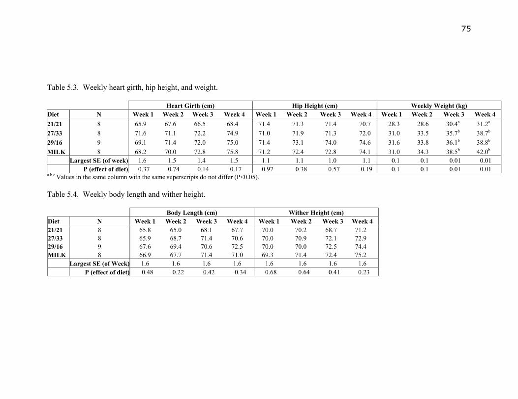
75
Table 5.3. Weekly heart girth, hip height, and weight. Heart Girth (cm) Hip Height (cm) Weekly Weight (kg) Diet N Week 1 Week 2 Week 3 Week 4 Week 1 Week 2 Week 3 Week 4 Week 1 Week 2 Week 3 Week 4 21/21 8 65.9 67.6 66.5 68.4 71.4 71.3 71.4 70.7 28.3 28.6 30.4a 31.2a 27/33 8 71.6 71.1 72.2 74.9 71.0 71.9 71.3 72.0 31.0 33.5 35.7b 38.7b 29/16 9 69.1 71.4 72.0 75.0 71.4 73.1 74.0 74.6 31.6 33.8 36.1b 38.8b MILK 8 68.2 70.0 72.8 75.8 71.2 72.4 72.8 74.1 31.0 34.3 38.5b 42.0b Largest SE (of week) 1.6 1.5 1.4 1.5 1.1 1.1 1.0 1.1 0.1 0.1 0.01 0.01 P (effect of diet) 0.37 0.74 0.14 0.17 0.97 0.38 0.57 0.19 0.1 0.1 0.01 0.01 a.b.c Values in the same column with the same superscripts do not differ (P<0.05). Table 5.4. Weekly body length and wither height. Body Length (cm) Wither Height (cm) Diet N Week 1 Week 2 Week 3 Week 4 Week 1 Week 2 Week 3 Week 4 21/21 8 65.8 65.0 68.1 67.7 70.0 70.2 68.7 71.2 27/33 8 65.9 68.7 71.4 70.6 70.0 70.9 72.1 72.9 29/16 9 67.6 69.4 70.6 72.5 70.0 70.0 72.5 74.4 MILK 8 66.9 67.7 71.4 71.0 69.3 71.4 72.4 75.2 Largest SE (of Week) 1.6 1.6 1.6 1.6 1.6 1.6 1.6 1.6 P (effect of diet) 0.48 0.22 0.42 0.34 0.68 0.64 0.41 0.23
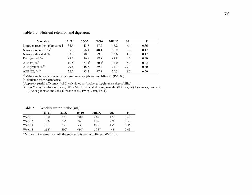
76 Table 5.5. Nutrient retention and digestion.
Variable 21/21 27/33 29/16 MILK SE P
Nitrogen retention, g/kg gained 33.4 43.8 47.9 46.2 6.4 0.36 Nitrogen retained, %A 39.1 56.1 40.4 56.9 5.3 0.12 Nitrogen digested, % 83.2 90.0 89.6 92.6 1.3 0.12 Fat digested, % 97.3 96.9 98.8 97.8 0.6 0.20 APE fat, %B 10.8a 27.1b 30.3b 37.0b 5.7 0.02 APE protein, %B 79.6 48.5 59.1 71.7 27.3 0.80 APE GE, %B,C 22.7 32.2 37.3 30.3 8.5 0.56 a,bValues in the same row with the same superscripts are not different (P<0.05). ACalculated from balance trial. BApparent partial efficiency (APE) calculated as (intake-gain)/(intake x digestibility). CGE in MR by bomb calorimeter, GE in MILK calculated using formula: (9.21 x g fat) + (5.86 x g protein) + (3.95 x g lactose and ash) (Brisson et al., 1957; Lister, 1971).
Table 5.6. Weekly water intake (ml). 21/21 27/33 29/16 MILK SE P
Week 1 310 573 380 234 170 0.60 Week 2 218 835 567 414 274 0.53 Week 3 313 539 733 603 138 0.35 Week 4 256a 492b 610b 274ab 46 0.03 abValues in the same row with the superscripts are not different (P<0.10).

77 Table 5.7. Gross energy content of body components.
Variable Baseline 21/21 27/33 29/16 MILK SE P CAR, %EBW 30.0 31.1 31.4 31.3 31.9 1.5 0.89 GE CAR, kcal/g 4.3a 4.5a 4.8ac 4.7ac 5.1bc 0.2 0.01 BO, %EBW 16.6a 18.6ab 20.8b 19.3ab 20.4ab 1.1 0.07 GE BO, kcal/g 5.3 5.2 6.0 5.3 5.2 0.3 0.07 HHFT, %EBW 53.4a 50.2ab 47.8b 49.4b 47.7b 1.0 <0.01 GE HHFT, kcal/g 4.0a 4.0a 4.5ab 4.4ab 4.9b 0.1 <0.01 a,b,cValues in the same row with the same superscripts are not different ( P<0.05). Carcass (CAR), Blood and organs (BO), Head, hide, feet, and tail (HHFT). Table 5.8. Composition of the empty body.
Variable Baseline 21/21 27/33 29/16 MILKA SE P Water, %EBW 65.4 58.4 58.8 58.7 57.6 3.6 0.44 Crude protein, %EBW 24.5 27.5 24.2 25.8 24.2 2.7 0.85 Ether extract, %EBW 2.8a 3.6a 6.8b 4.7a 8.2b 0.6 <0.01 Crude ash, % EBW 6.0 7.0 6.3 6.1 5.4 0.6 0.45 EBW, kg 24.9a 29.3b 37.1c 35.8c 35.5c 1.2 <0.01 GE EB initial, Mcal 37.5 40.2 41.9 40.5 36.0 2.0 0.19 GE EB final, Mcal 45.8a 66.6b 59.6a 69. 0b 5.9 0.02 GE gained, Mcal 6.9a 25.6b 20.1b 33.3b 5.9 0.02 a,bValues in the same row with the same superscripts are not different (P<0.05). A for MILK GE calculated; GE = (9.21 x g fat) + (5.86 x g protein) + (3.95 x g lactose and ash) (Brisson et al., 1957; Lister, 1971).

78
Table 5.9. Changes in body composition. Variable 21/21 27/33 29/16 MILK SEM P
Water gained, kg 1.32 4.37 4.75 5.48 1.53 0.16 Protein gained, kg 1.43 1.98 2.54 2.93 1.06 0.69 Fat gained, kg 0.16a 1.69b 0.83a 2.38b 0.24 <0.01 Ash gained, kg 0.46 0.62 0.57 0.54 0.23 0.95 a,bValues in the same row with the same superscripts are not different (P<0.05).

79
Average Daily Gain
0.110
0.496
0.3680.357
0.00
0.05
0.10
0.15
0.20
0.25
0.30
0.35
0.40
0.45
0.50
0.55
20/20 27/33 29/16 Milk
Diet
AD
G (k
g)
Figure 5.1. Average daily gains.

80

81
Weight Gained
13.9
10.310
3.1
0
2
4
6
8
10
12
14
16
20/20 27/33 29/16 Milk
Diet
Wei
ght g
aine
d (k
g)
Figure 5.2. Total weight gained by diet.

82
Weekly Weight
0
5
10
15
20
25
30
35
40
45
50
1 2 3 4
Week
Wei
ght,
kg
20/20
27/33
29/16
Milk
Figure 5.3. Weekly weight.
Linear effect of diet P<0.0001

83
Weekly Hip Heights
64
66
68
70
72
74
76
78
1 2 3 4
Week
Hei
ght,
cm
20/20
27/33
29/16
Milk
Figure 5.4. Weekly hip height.

84
Weekly Body Length
58
60
62
64
66
68
70
72
74
76
1 2 3 4Week
Leng
th, c
m
20/20
27/33
29/16
Milk
Figure 5.5. Weekly body length.

85
W eeky W ither Heights
62.0
64.0
66.0
68.0
70.0
72.0
74.0
76.0
78.0
1 2 3 4
W eek
Hei
ght,
cm
20/20
27/33
29/16
Milk
Figure 5.6. Weekly wither height.
The week by diet interaction was significant (P<0.04).

86
Weekly Heart Girth
40
45
50
55
60
65
70
75
80
1 2 3 4
Week
Hei
ght,
cm
20/20
27/33
29/16
Milk
Figure 5.7. Weekly hearth girth.
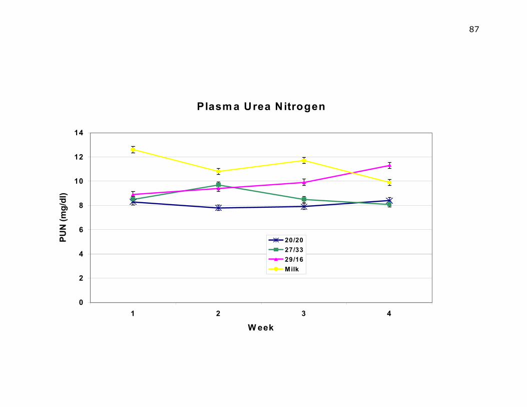
87
Plasm a Urea Nitrogen
0
2
4
6
8
10
12
14
1 2 3 4
W eek
PUN
(mg/
dl)
20/2027/3329/16Milk

88 Figure 5.8. Weekly plasma urea nitrogen.
Plasma Glucose
80
85
90
95
100
105
110
115
120
125
130
1 2 3 4
Week
Glu
cose
(mg/
dl)
20/2027/3329/16Milk
Figure 5.9. Weekly plasma glucose.

89

90
NEFA
0
100
200
300
400
500
600
700
800
1 2 3 4Week
NEF
A (m
Eq/l)
20/2027/3329/16milk
Figure 5.10. Weekly NEFA.

91
��������������������������������������������������������������������������������������������������������������������������������������������������������������������
�������������������������������������������������������������������������������������������������������������������������������������������������������������������������������������������������������������������������������������������������������������������������
����������������������������������������������������������������������������������������������������������������������������������������������������������������������������������������������������������������������������������������������������������������������������������������������������������������������������������������������������������������������������������������������������������������������������������������������������������������������������������������������������������
����������������������������������������������������������������������������������������������������������������������������������������� �������������������������������������������������������������������� ���������������������������������������������������������������������������������������������������������������������������������������
���������������������������������������������������������������������������������������������������������������������������������������������������������������������������������������������������������������������������������������������������������������������������������������������������������������������������������������������������������������� �����������������������������������������������������������������������������������������������������������������������������������������������������������������������������������������������������������������������������������������
Percentage Fat in Empty Body
0.0%
1.0%
2.0%
3.0%
4.0%
5.0%
6.0%
7.0%
8.0%
9.0%
10.0%
Baseline 20/20 27/33 29/16 MilkDiet
Fat
(%)
a
a
a
b
b
Figure 5.11. Percentage fat in empty body.

92

93
������������������������������������������������������������������������������������������������������������������������������������������������������������������������������������������������������������������
������������������������������������������������������������������������������������������������������
������������������������������������
���������������������������������������������������������������������������������������
���������������������������������������������������������������������� �����������������������������������������������������������������������������������������������������������������������������������������
���������������������������������������������������������������������������������������������������������������������������������������������
������������������������������������
������������������������������������������������
������������������������������������������������������������������������������������������������������������������������������������������������������������������������������������������������������������
���������������������������������������������������������������������������������������������������������������
������������������������
���������������������������������������������������������������������������������������������
Com position of Em pty Body W eight Gain
-0.1
0.1
0.3
0.5
0.7
0.9
%water %protein %ash %fat
% o
f em
pty
body
gai
n
20/20
������ 27/33
����� 29/16������ M ilk
Figure 5.12. Composition of empty body weight gain.

94
�������� ������� ������������������������������������������������������������������������������������������������������������������������������������������������������������������������ ���������������������������� ��������������������� �������������
������������������������������������������������������������������������������������������������������������������������������������������������������������������������������������������������
������������������������������������������������������������������������������������������������������������������������������������������������������������������������������������������������
������������������������������������������������������������������������������������������������������������������������������������������������������������������������������������������������
������������������������������������������������������������������������������������������������������������������������������������������������������������������������������������������������
������������������������������������������������������������������������������������
������������������������������������������������������������������������������������������
������������������������������������������������������������������������������������
������������������������������������ ��������������������� ��������������������� ���������������������������
����������������������������� ��������������������� ��������������������� ���������������������������
������������������������
������������������������������
����������������������������
������������������������
������������������������
���������������������
���������������������
������������������������������
������������������������
������������������������������������
Empty Body Composition
65.0%
58.0%
59.0%
59.0%
58.0%
24.0%
27.0%
24.0%
26.0%
24.0%
6.0%
7.0%
6.0%
6.0%
6.0%
3.7%
2.9%
8.3%
4.8%
6.9%
0.0% 10.0% 20.0% 30.0% 40.0% 50.0% 60.0% 70.0% 80.0%
Baseline
20/20
27/33
29/16
Milk
% of Body
���������� Water
���������� Protein
���������� Ash���������� Fat
Figure 5.13. Empty body composition.

95
Weekly Fecal Scores
0
0.5
1
1.5
2
2.5
3
1 2 3 4
Week
Ave
rage
Wee
kly
Feca
l Sco
re
20/20
27/33
29/16
Milk

96 Figure 5.14. Weekly fecal scores.
1 2 3 4 5 6 7 8 9
������������������������������������������������������������������������������������������������������������������������������������������������������������������������������������������������������������������������������������������������������������������������������������������������������������������������������������������������������
������
���������
����������������������������������������������������������������������������������������������
��������� ����������������������������������������������������������������������������������������������
��������� �������������������������������������������������������������������������������������������������
��������� �������������������������������������������������������������������������������������������������
���������
������
����������������������������������������������������������������������������
����
���������
��������������������������������������������������������������������������������������������������������������������������������������������������������������������������
������
��������� ��������� ���������
�����������������������������������������������������������������������������������������
���������
�����������������������������������������������������������������������������������������������������������������������������������������������������������������������������
������ �������������������������������������������������������������������������������������������������������������������������������������
����
����������������������������������������������������������������������������������������������
��������� �����������������������������������������������������������������������������������������
���������
�������� ��������� ���������
��������������������������������������������������������������������������������������������������������������������������������������������������������������������������������������������������������������������������������������������������������������������������������������������������������
������
���������
��������������������������������������������������������������������������������������������������������������������������������������������������������������������������������������������������������������������������������������������������������������������������������������������������������������������������������������������������������������������������������������������������������������������
����
������ ���������
�������������������������������������������������������������������������������
������
�������������������������������������������������������������������������������������������������������������������������������������������������������������������������������������������������������������������������������������������������������
��������� �������������������������������������������������������������������������������������������������������������������������������������������������������������������������������������������������������������������������������������������������������
���������
�������� ��������� ����
��������
���������������������������������������������������������������������������������������������������������
��������� ��������������������������������������������������������������������������������������������������������������
��������� ����������������������������������������������������������������������������������������������������������
��������� ��������������������������������������������������������������������������������������������������������������
���������
0 .0 %
5 .0 %
1 0 .0 %
1 5 .0 %
2 0 .0 %
2 5 .0 %
3 0 .0 %
3 5 .0 %
4 0 .0 %
4 5 .0 %
5 0 .0 %
% o
f cal
ves
M e d ic a tio n d a ys
D is tr ib u tio n o f M e d ic a tio n D a ys b y D ie t
���������� 20 /20
�������� 27 /33
���������� 29 /16
�������� M ilk
Figure 5.15. Distribution of medication days.
On the x-axis the total number of days of medication or electrolyte therapy are shown. On the y-axis the the % of calves per diet are
shown.

97
Chapter Six
Usefulness of Dual X-ray Absorptiometry for Analyzing Composition of
Calf Tissues.
Results and Discussion
Table 6.1 details the nutrient concentration of diets fed. Table 6.2 summarizes total
nutrient intake of calves during the 26-d feeding period. Dual energy x-ray absorptiometry
(DXA) detected differences in body composition (Table 6.3). According to DXA
estimates, percentage bone mineral content (BMC) in the carcass (CAR) was greater in
MILK than 21/21 and 29/16. Calves fed MILK and baseline had the lowest percentage
lean in CAR. Percentage fat in the blood and organs (BO) was least in calves fed 21/21 or
29/16. No differences in BMC, percentage lean tissue, or percentage fat, due to diet were
detected by DXA in the liver.
Correlations between body composition as predicted by DXA and chemical analysis
(CHEM) are shown in Figures 6.1 to 6.6. Estimates of body composition by DXA were
poorly correlated to CHEM (adjust R-square <0.1). The reasons for the inaccurate
estimates of composition by DXA are not clear. This technology has been used
successfully to estimate the composition of pigs. Mitchell et al. (1998a) reported higher
correlations between DXA and CHEM estimates of percentage fat (r=0.89) and grams of
fat (r=0.96) in the eviscerated body of pigs weighing between 5 and 27 kg.
Estimates of tissue mass, i.e., weight by DXA were more accurate than estimates of
composition. Figures 6.7 to 6.9 show the relationship between DXA estimates of mass
and mass as measured by a scale. In particular, the DXA estimate of liver mass was very
close to the scale weight (adjust. R-square= 0.99). The DXA estimates of mass, i.e.,
weight, of calf tissues are in agreement with values reported for pigs. Mitchell et al.
(1998b) reported a high correlation (r > 0.99) between DXA estimates of mean carcass
weight in pigs and the scale weight of carcasses.

98
Differences in body composition due to diet as detected by DXA and CHEM varied (Table
6.4). According to DXA, percentage fat in CAR was highest in baseline calves and calves
fed MILK. However, CHEM detected a much lower percentage fat in CAR of baseline
calves than DXA. Chemical analysis indicated that MILK and 27/33 had greatest
percentage fat in CAR and baseline calves had the lowest. In the blood and organs, both
CHEM and DXA detected greatest percentage fat in calves fed 27/33 and MILK.
However, DXA estimates indicated that baseline calves had a similar percentage fat in the
BO as calves fed 27/33 and MILK but CHEM had a considerably lower estimate of fat in
baseline calves than DXA. Estimates of percentage fat in the BO and CAR baseline calves
and calves fed 21/21 were higher than CHEM and may indicate that DXA overestimates
percentage fat in lean animals (Table 6.4). Research with pigs has shown that DXA
significantly underestimates the percentage fat in the carcass by up to 28% (Mitchell et al.,
1998b). The reasons for discrepancies between CHEM and DXA in detection of body
composition of tissue from baseline calves may have been the small sample size (n=2) or
the smaller mass of tissues from baseline calves, or may be related to limitations of the
DXA equipment. More research with a larger sample size should be conducted to
determine the accuracy of DXA in estimating body composition in live calves.
Conclusions
DXA accurately estimated the mass of tissues from calves but was a poor predictor of body
composition. However, refinements in the procedure, calibration, and technique may
allow DXA estimates to more closely approach CHEM measurements of body composition
in calves. Additional studies of accuracy using DXA to estimate body composition in
calves are merited.

99 Table 6.1. Diet specifications on an as fed (powder) basis.
Variable 21/21 27/33 29/16 MILK
DM, % 97.3 97.3 97.3 14.0A Crude protein, % 20.6 27.3 28.5 3.5 Crude fat, % 20.6 33.4 16.4 4.8 Lactose+ash, % 58.8B 39.3B 55.1B 5.7B Crude fiber, % 0.15 0.15 0.15 Calcium, % 0.90 0.90 0.90 Phosphorus, % 0.70 0.70 0.70 Iron, ppm 100 100 100 Copper, ppm 10 10 10 Cobalt, ppm 0.1 0.1 0.1 Zinc, ppm 40 40 40 Manganese, ppm 40 40 40 Iodine, ppm 1.02 1.02 1.02 Selenium, ppm 0.30 0.30 0.30 Vitamin A, IU/kg 9091 9091 9091 Vitamin D3, IU/kg 2273 2273 2273 Vitamin E, IU/kg 45 45 45 Thiamine, mg/kg 6.61 6.61 6.61 Riboflavin, mg/kg 6.61 6.61 6.61 Niacin, mg/kg 2.64 2.64 2.64 d-Pantothenic Acid, mg/kg 13.22 13.22 13.22 Biotin, mg/kg 0.11 0.11 0.11 Ascorbic Acid, mg/kg 110.00 110.00 110.00 Pyridoxine Hydrochloride, mg/kg 6.61 6.61 6.61 Folic Acid, mg/kg 0.55 0.55 0.55 Vitamin B12, mg/kg 0.07 0.07 0.07 Choline Chloride, mg/kg 1322.0 1322.0 1322.0 AEstimated. BLactose + Ash determined by difference.

100
Table 6.2. Total nutrient intake and performance of calves by diet.
Variable 21/21 27/33 29/16 MILK SE Number of calves 5 5 4 3 Liquid fed, kg 88.1a 145.8b 144.0b 138.6c 1.9 DM fed, kg 11.0a 18.2b 18.0b 19.4c 2.5 Protein fed, g 2264a 4973b 5132bc 4904b 61.1 Fat fed, g 2272a 6089a 2954d 6683c 71.0 a,b,c,dValues in the same row with similar superscripts do not differ at p<0.05.
Table 6.3 Composition of tissues as estimated by DXA. Variable Baseline 21/21 27/33 29/16 MILK SE
DXA %BMC CAR 0.44ab 0.27a 0.46ab 0.26a 0.67b 0.01 DXA %Lean CAR 79.3a 87.0b 85.5b 86.9b 84.1a 1.3 DXA % fat CAR 20.8a 12.8b 13.9b 12.6b 15.8ab 1.4 DXA %fat BO 15.4a 13.0b 14.8a 13.7b 15.4a 0.8
abValues in the same row with similar superscripts do not differ at p=0.05 Table 6.4 Composition of tissues estimated by DXA or CHEM.
Variable Baseline 21/21 27/33 29/16 MILK SE DXA CAR %fat 20.8a 12.8b 13.9b 12.6b 15.8ab 1.4 CHEM CAR %fat 4.0a 9.2ac 22.5b 13.9c 22.4b 2.1 DXA BO %fat 15.4a 13.0b 14.8a 13.7b 15.4a 0.8 CHEM BO %fat 7.6a 11.0a 27.0b 15.9a 28.4b 2.9
abValues in the same row with similar superscripts do not differ at p=0.05


102 Figure 6.1 Chemical analysis of percentage ash in the carcass versus DXA estimates of percentage bone mineral content.
Legend: A = 1 obs, B = 2 obs, etc. ‚ Ch Carash = 0.571 0.02602 DXA_half_BMC adjust. R-square =-0.056 0.8 ˆ ‚ ‚ A ‚ 0.7 ˆ A A ‚ A c ‚ A h ‚ B _ 0.6 ˆ A A c ‚ a ‚ A r ‚ A a 0.5 ˆ A A s ‚ A A h ‚ A A ‚ A 0.4 ˆ A ‚ ‚ ‚ 0.3 ˆ ‚ Šƒƒˆƒƒƒƒƒƒƒƒˆƒƒƒƒƒƒƒƒˆƒƒƒƒƒƒƒƒˆƒƒƒƒƒƒƒƒˆƒƒƒƒƒƒƒƒˆƒƒƒƒƒƒƒƒˆƒƒƒƒƒƒƒƒˆƒƒƒƒƒƒƒƒˆƒƒƒƒƒƒƒƒˆƒƒ 0.0 0.1 0.2 0.3 0.4 0.5 0.6 0.7 0.8 0.9 DXA_half_BMC

103
Figure 6.2 Chemical analysis of carcass percentage protein versus DXA estimates of percentage lean tissue in carcass.
Legend: A = 1 obs, B = 2 obs, etc. ‚ Ch carprotein = 69.30 + 1.61 DXA_h_lean adjust R-square = -0.044 300 ˆ ‚ ‚ ‚ c ‚ A A A h 250 ˆ A A _ ‚ A c ‚ a ‚ A A r ‚ A A A p 200 ˆ r ‚ A A A o ‚ A t ‚ A e ‚ A i 150 ˆ n ‚ A A ‚ ‚ ‚ 100 ˆ ‚ Šƒƒˆƒƒƒƒƒƒƒƒƒƒƒˆƒƒƒƒƒƒƒƒƒƒƒˆƒƒƒƒƒƒƒƒƒƒƒˆƒƒƒƒƒƒƒƒƒƒƒˆƒƒƒƒƒƒƒƒƒƒƒˆƒƒƒƒƒƒƒƒƒƒƒˆƒƒƒƒƒƒƒƒƒƒƒˆƒƒ 76 78 80 82 84 86 88 90 DXA_h_Lean

104 Figure 6.3 Chemical analysis of percentage water in carcass versus DXA estimate of percentage lean tissue.
Legend: A = 1 obs, B = 2 obs, etc. ‚ Ch_carwater = 7.82 - 0.009DXA_h_lean Adjust. R-square = -0.058 9 ˆ ‚ ‚ A ‚ A A 8 ˆ A A c ‚ A AA h ‚ A _ ‚ A A c 7 ˆ A A a ‚ r ‚ A A w ‚ a 6 ˆ A t ‚ e ‚ r ‚ 5 ˆ A A ‚ A ‚ ‚ 4 ˆ ‚ Šƒƒˆƒƒƒƒƒƒƒƒƒƒƒˆƒƒƒƒƒƒƒƒƒƒƒˆƒƒƒƒƒƒƒƒƒƒƒˆƒƒƒƒƒƒƒƒƒƒƒˆƒƒƒƒƒƒƒƒƒƒƒˆƒƒƒƒƒƒƒƒƒƒƒˆƒƒƒƒƒƒƒƒƒƒƒˆƒƒ 76 78 80 82 84 86 88 90 DXA_h_Lean

105 Figure 6.4 Chemical estimate of percentage fat in carcass versus DXA estimate of %fat.
Legend: A = 1 obs, B = 2 obs, etc. ‚ Ch_pct_fat = 12.01 + 0.225DXA_h_Fat Adjust R-square = -0.052 30 ˆ ‚ A ‚ c ‚ h ‚ A A A _ ‚ p ‚ c 20 ˆ A A A t ‚ A A _ ‚ f ‚ a ‚ A t ‚ A _ ‚ c 10 ˆ A A A a ‚ A A r ‚ A ‚ ‚ A A ‚ ‚ 0 ˆ Šƒƒˆƒƒƒƒƒƒƒƒƒƒƒƒƒˆƒƒƒƒƒƒƒƒƒƒƒƒƒˆƒƒƒƒƒƒƒƒƒƒƒƒƒˆƒƒƒƒƒƒƒƒƒƒƒƒƒˆƒƒƒƒƒƒƒƒƒƒƒƒƒˆƒƒƒƒƒƒƒƒƒƒƒƒƒˆƒƒ 10 12 14 16 18 20 22 DXA_h_Fat

106 Figure 6.5 Chemical analysis of percentage water in blood and organs versus DXA estimate of percentage lean.
Legend: A = 1 obs, B = 2 obs, etc. ‚ Ch_pct_water_bo = 438.6 -4.43dxa_o_lean Adjust. R-Square = 0.06 100 ˆ ‚ ‚ c ‚ h ‚ A A _ 80 ˆ A A A A p ‚ c ‚ t ‚ A _ ‚ w 60 ˆ A A a ‚ A A t ‚ e ‚ r ‚ A A A A _ 40 ˆ A A b ‚ A A o ‚ ‚ ‚ 20 ˆ ‚ Šƒƒˆƒƒƒƒƒƒƒƒƒƒƒƒƒˆƒƒƒƒƒƒƒƒƒƒƒƒƒˆƒƒƒƒƒƒƒƒƒƒƒƒƒˆƒƒƒƒƒƒƒƒƒƒƒƒƒˆƒƒƒƒƒƒƒƒƒƒƒƒƒˆƒƒƒƒƒƒƒƒƒƒƒƒƒˆƒƒ 82 83 84 85 86 87 88 dxa_o_lean

107 Figure 6.6 Chemical analysis of percentage protein in blood and organs versus DXA estimate of percentage lean.
Legend: A = 1 obs, B = 2 obs, etc. ‚ Ch_pct_pro = 34.7 +.81dxa_o_lean Adjust R-square = 0.042 90 ˆ ‚ ‚ A A ‚ c ‚ A A A h 80 ˆ A A _ ‚ A A p ‚ c ‚ t ‚ _ 70 ˆ A A A p ‚ A A r ‚ A o ‚ A _ ‚ A A b 60 ˆ o ‚ ‚ A ‚ ‚ 50 ˆ ‚ Šƒƒˆƒƒƒƒƒƒƒƒƒƒƒƒƒˆƒƒƒƒƒƒƒƒƒƒƒƒƒˆƒƒƒƒƒƒƒƒƒƒƒƒƒˆƒƒƒƒƒƒƒƒƒƒƒƒƒˆƒƒƒƒƒƒƒƒƒƒƒƒƒˆƒƒƒƒƒƒƒƒƒƒƒƒƒˆƒƒ 82 83 84 85 86 87 88 dxa_o_lean

108 Figure 6.7 Organ mass versus DXA estimate of organ mass.
Legend: A = 1 obs, B = 2 obs, etc. ‚ O_chemass = 753.5 + 1.36 O_dxamass adjust. R-square = 0.62 10000 ˆ ‚ ‚ ‚ A ‚ ‚ A o ‚ _ 8000 ˆ c ‚ h ‚ A e ‚ A m ‚ A A A A A a ‚ A s ‚ s 6000 ˆ A ‚ A ‚ A A ‚ A A ‚ ‚ B ‚ A 4000 ˆ Šƒˆƒƒƒƒƒƒƒƒƒƒƒˆƒƒƒƒƒƒƒƒƒƒƒˆƒƒƒƒƒƒƒƒƒƒƒˆƒƒƒƒƒƒƒƒƒƒƒˆƒƒƒƒƒƒƒƒƒƒƒˆƒƒƒƒƒƒƒƒƒƒƒˆƒƒƒƒƒƒƒƒƒƒƒˆƒ 2500 3000 3500 4000 4500 5000 5500 6000 o_dxamass

109 Figure 6.8 Liver mass versus DXA estimate of liver mass.
Legend: A = 1 obs, B = 2 obs, etc. ‚ L_chemass = -2.82 + 0.98L_dxamass Adjust R-square = 0.99 1000 ˆ ‚ A ‚ A ‚ A ‚ A A ‚ A A l ‚ A A _ 800 ˆ A c ‚ h ‚ A e ‚ A m ‚ A a ‚ A s ‚ A s 600 ˆ ‚ ‚ A ‚ A ‚ A ‚ A ‚ 400 ˆ Šƒˆƒƒƒƒƒƒƒƒƒƒƒƒƒˆƒƒƒƒƒƒƒƒƒƒƒƒƒˆƒƒƒƒƒƒƒƒƒƒƒƒƒˆƒƒƒƒƒƒƒƒƒƒƒƒƒˆƒƒƒƒƒƒƒƒƒƒƒƒƒˆƒƒƒƒƒƒƒƒƒƒƒƒƒˆƒƒ 400 500 600 700 800 900 1000 l_dxamass
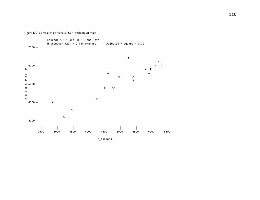
110 Figure 6.9 Carcass mass versus DXA estimate of mass.
Legend: A = 1 obs, B = 2 obs, etc. ‚ H_chemass= 1297 + 0.78h_dxamass Adjusted R-square = 0.79 7000 ˆ ‚ ‚ ‚ A ‚ A 6000 ˆ A A h ‚ A A _ ‚ A A c ‚ A A h ‚ A e 5000 ˆ m ‚ B AA a ‚ s ‚ s ‚ A 4000 ˆ A ‚ ‚ A ‚ ‚ A 3000 ˆ ‚ Šƒƒˆƒƒƒƒƒƒƒƒƒˆƒƒƒƒƒƒƒƒƒˆƒƒƒƒƒƒƒƒƒˆƒƒƒƒƒƒƒƒƒˆƒƒƒƒƒƒƒƒƒˆƒƒƒƒƒƒƒƒƒˆƒƒƒƒƒƒƒƒƒˆƒƒƒƒƒƒƒƒƒˆƒƒ 2500 3000 3500 4000 4500 5000 5500 6000 6500 h_dxamass
111
Chapter Seven
Jersey calf management practices in the United States
Results and Discussion
Characteristics of herds Herds surveyed reported 20,806 births in the 12 mo prior to the survey, of these 19,303
were Jersey calves. Only three of the herds survey reported less than 50% of births on
their farm as Jersey calves. Jersey herds enrolled in American Jersey Cattle Association
(AJCA) performance programs averaged 7023 kg of milk, 323 kg fat, and 251 kg of
protein, actual production in 2001 (Wolfe, 2001b). Herds surveyed were representative of
the US population in terms or production, averaging 7180 ±757 kg of milk, 331 ±37 kg of
fat, and 256 ± 29 kg of protein, actual production. Table 7.1 summarizes the
characteristics of all herds surveyed, the top ten percent of herds, and herds by region. The
difference between the average and the top 10% of herds in each category indicates that the
herds were diverse. Culling rate averaged 27.5 ±12.5% but herds in the tenth percentile for
culling rate culled less than 11%. Over half (56%) of herds sold cows for dairy purposes.
Herds surveyed sold an average of 7.8 ±12.0% of the herd for dairy purposes while the
tenth percentile sold over 21%. Calving interval averaged 13.0 ±0.7 mo. and somatic cell
count (1000s) averaged 232 ±111. The top herds had a calving interval of 12.2 mo and
herds and the top 10% of herds had an average SCC of less than 78,000. Herds reported
an average of 199 calves born while herds in the 90th percentile averaged 430 births.
Herds surveyed had similar milk production, culling rate, and calving interval, and SCC
regardless of region. However, herds in the WEST had the most births (582) and the
highest level of milk production (7530 kg). Herds in the NEAST had the fewest births
(70). Herd size differences due to region were similar to those reported by NAHMS,
(1996a).

112 Calf mortality in the first 24 hours of life including stillbriths (M24) averaged 5.0% with
the highest in PAOHIN (5.9%) and the lowest in NEAST (3.9%). The majority of herds
in the NEAST utilized maternity pens for calving cows (Table 7.2), which may indicate
prepartum cows, and newborn calves are managed more intensively due to their close
proximity to the milking herd. The level of early calf mortality in the US Jersey
population appears to be lower than the Holstein population. Adamec, (2002) reported calf
mortality from birth to 48 h of age, including stillbirths, in the US Holstein population
exceeds 7%. Winston, (1998) reported 7.1% early calf mortality (calves born dead or that
died soon after birth) in PA Jersey herds, which was slightly more than observed in the
current survey for PAOHIN and for the United States and may indicate a slight decline in
early calf mortality in Jersey herds.
Mortality between 24 h of age and 3 mo (M3) averaged 6.7% (Table 7.2) which is lower
than reported by Winston (1998) in PA Jersey herds (8.1%) or NAHMS (1996b) (11.0%).
The NAHMS, (1996b) data was predominantly from Holstein herds (93% of the data).
Level of mortality in the United States increased from 8.4% in 1992 to 11.0% in 1996
(NAHMS, 1996b). However, the current level of Jersey calf mortality appears to be
decreasing when compared to the data reported by Winston, (1998). This could indicate
that Jersey breeders are making improvements in the management and care of calves and
may indicate that Jersey breeders are more aggressive managers of calves than the typical
United States dairy herd.
Mortality after 3 mo of age averaged 1.3% and was slightly higher than the 0.5% reported
by Winston (1998). Mortality was highest in the SEAST was (2.3%) and may reflect a
less intensive system of managing heifers that utilizes more pasture and less confinement
for rearing heifers after 3 mo of age. Mortality in NEAST was lower than average (0.7%).
Calving location is another important factor in calf management. Calving location varied
considerably within region and by region (Table 7.2). The majority of respondents used
more than one location to calve cows, depending on the season of the year and the number

113 of cows calving. Only 46% of respondents allowed cows to calve in a pasture but the
variation was considerable with only 17% of the respondents in the NEAST utilizing
pasture and 69% of respondents in the SEAST utilizing pasture. Regional variation in
housing for maternity cows varied considerably across regions; 43% in SEAST to 74.5%
in WIS used maternity pens as a location to calve cows. Loose housing barns were only
used in the WEST and in PAOHIN as a calving location.
Management of newborns
Feeding an adequate amount of high quality colostrum to the newborn calf is critical to
successful calf rearing. Colostrum should be fed soon after birth and then 12 h later. At
least 1.9 L of colostrum should be fed per feeding (Roy, 1980). Overall, respondents
delivered an adequate quantity of colostrum in a timely matter (Table 7.2). Average time
to first colostrum feeding was 3.8 h after birth and on average 1.9 L of colostrum was fed
at the first feeding. Respondents reported feeding 3.8 L of colostrum in the first 24 h of
life. Timing of first colostrum feeding was comparable to NAHMS (1993), which reported
68.6% of herds fed the first feeding of colostrum in the first 6 h of life. Only 11% of
producers depended on nursing for colostrum delivery. Nursing was most often used as a
method of colostrum delivery in the SEAST where 31% of producer reported allowing
calves to nurse. The higher level of nursing in the SEAST is likely related to extensive use
of pasture as a calving location. The NAHMS (1996b) survey reported 33.5% of dairy
producers relied on the calf to nurse for first feeding of colostrum, which is higher than
observed among Jersey breeders.
Calf nutrition and management
Calf nutrition and management practices are summarized in Table 7.3. Respondents fed a
variety of liquid diets to preweaned calves and 15% of respondents fed more than one
source of liquid to calves. Producers may have changed source of liquid feed depending
on season of year, others may have transitioned individual calves from one source of liquid
to another, and others may have switched from one source of liquid to another based on

114 price and availability. The majority (57%) of respondents fed MR, 25% of respondents fed
waste milk, and 47% of respondents fed salable milk. Feeding raw milk is a concern due
to the risk of disease transmission (Cullor, 2000) and the presence of antibiotics in waste
milk (Selim and Cullor, 1997). Use of milk and waste milk as calf feeds indicates that
Jersey breeders are willing to assume risks associated with feeding waste milk, are
unaware of these risks, and/or they perceive benefits from feeding these feeds.
Transmission of Johne’s disease in raw milk is also a concern and pasteurization has been
recommended as a method of reducing the risk of transmitting Johne’s disease in milk
(Stabel, 2000). Only producers in the WEST fed pasteurized milk. Producers that fed milk
reported feeding 3.1 kg of milk/calf/d while producers that fed MR reported feeding 440g
of powder/calf/d. For a 27 kg calf, this is an as fed feeding rate of approximately 12% of
BW. Larger frame calves are typically fed liquid at 8 to 10% of BW (Davis and Drackley,
1998). In addition to being fed more liquid, Jersey calves were weaned one week later
than reported by NAHMS (1996b), i.e. 9.4 versus 8.4 wk. However, average age at
weaning varied 3 wk by region with the lowest at 7.8 weeks in WIS and the greatest was
10.8 wk in WEST. Average age for weaning is considerably higher than the 35 d
suggested by Quigley (1996) indicating that Jersey breeders could wean calves sooner.
Water is an important component of the calf’s diet. Average age water was first offered to
calves, among herds that offered water, was 9.8 d. Only 73% of respondents offered water
to calves before weaning. Davis and Drackley (1998) recommended preweaned calves
have fresh water available at all times. Herds in the SEAST were least likely to offer
water supplied to preweaned calves while 100% of the herds in WIS offered water to
calves. Producers may be reluctant to offer water to calves due to effort involved in
keeping clean fresh water to calves or producers may not be aware of the importance of
offering water to calves. When calves begin to scour, water intake increases (Kertz et al.,
1984). Given the importance of water intake to the preweaned calf and relative ease of
implementing this practice one would expect nearly 100% of producers would offer water
to calves before weaning. However, only 73% of producers offering water to calves
indicates this is an area where calf management could be improved.

115
Intake of calf starter is critical for rumen development (Warner et al., 1956). Calf starter
was offered to calves at an average age of less than 8 d (Table 7.3). The variation between
regions was small. Herds in NEAST offered starter to calves at an earlier age (6.5 d) than
other regions while herds in the SEAST waited the longest to offer calf starter (9.8 d).
Herds reported an average starter intake of 1.5 kg/d at weaning with little variation
between region indicating that calves should have had well-developed rumens when they
were weaned. Overall, Jersey breeders do an adequate job with calf starter management.
In addition to feeding liquid and calf starter to calves, over 50% of the herds offered some
type of forage prior to weaning (Table 7.3). Herds located in PAINOH and the SEAST
were least likely to feed forage before weaning and herds in NEAST and WEST were
more likely to feed forage before weaning. Herds in NEAST and WEST also had a higher
average age at weaning. These herds may use a more gradual method of weaning calves
that includes feeding forage a week or so before weaning and could partially account for
the higher rate of forage feeding prior to weaning.
Health and reproduction
The majority of respondents had a routine herd health program with their veterinarian
(Table 7.4). Vaccination and disease prevention were a priority with 90% of herds
reporting some type of vaccination program for the milking herd and 85% of herds
vaccinated heifers. However, there was considerable variation in the vaccinations used.
Only 42% of the herds surveyed dewormed the milking herd but 66% of herds dewormed
heifers. Regional variation in deworming was considerable and was probably related to the
use of pasture in each region. The majority of herds (90%) used some form of coccidia
control. Respondents were aggressive in breeding heifers and reported a goal for average
age at first calving of less than 23 mo. In the WEST, the goal for age at first calving was
less than 22 mo.
Characteristics of primary calf feeder

116
The majority, 81% of respondents listed the owner (48%) or spouse (33%) as the primary
calf feeder (Table 7.5). In previous studies, lower calf mortality was observed when the
primary calf feeder was a female or the herd owner (Hartman et al., 1974; James et al.,
1984). However, the relationship between primary calf feeder and mortality was negligible
except that in herds where a child was the primary calf feeder, the incidence of mortality
(M24) was increased (Table 7.6). This may indicate that more emphasis is placed on calf
rearing than in the past. Perhaps the primary calf feeder has more skill, education, and
dedication to calf rearing than in the past. Some farms, particularly larger farms, may
have an employee whose primary responsibility is managing calves. Future studies should
further examine the characteristics including education and job responsibilities of the
primary calf feeder.
Mortality in the first 24 hours of life
Calving location is correlated with mortality (M24) (Table 7.6). Herds that utilize pasture
as a calving location had a higher incidence of mortality (M24). The higher level of
mortality in these herds may have been do to less intensive management of the maternity
cows. Herds that used a bedding material other than sawdust or straw in the maternity
area had a lower incidence of mortality (M24). These herds varied considerably in the
source of bedding used but the low level of mortality indicates these herds provided a
superior environment for the newborn calf. The higher incidence of mortality when
heifers calve in tie stalls indicates that tie stalls are a less than ideal form of housing for
heifers.
In addition to providing a superior calving environment herds with lower levels of
mortality (M24) fed more milk to calves, used BovatecTM to control coccidiosis, balanced
rations for dry cows, had a lower goal for age at first calving, and had higher rolling herd
average for milk production (Table 7.6). These factors are indicators of level of herd
management as is level of calf mortality (M24).
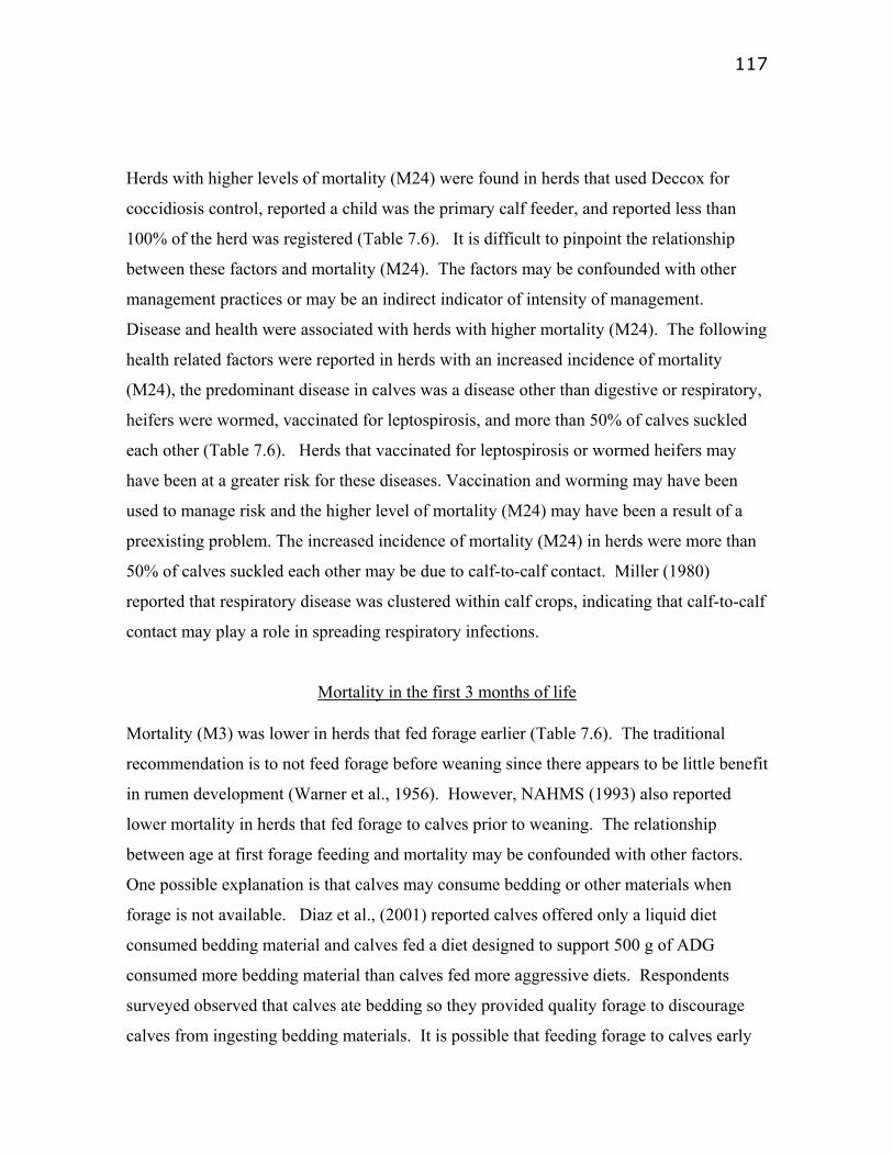
117
Herds with higher levels of mortality (M24) were found in herds that used Deccox for
coccidiosis control, reported a child was the primary calf feeder, and reported less than
100% of the herd was registered (Table 7.6). It is difficult to pinpoint the relationship
between these factors and mortality (M24). The factors may be confounded with other
management practices or may be an indirect indicator of intensity of management.
Disease and health were associated with herds with higher mortality (M24). The following
health related factors were reported in herds with an increased incidence of mortality
(M24), the predominant disease in calves was a disease other than digestive or respiratory,
heifers were wormed, vaccinated for leptospirosis, and more than 50% of calves suckled
each other (Table 7.6). Herds that vaccinated for leptospirosis or wormed heifers may
have been at a greater risk for these diseases. Vaccination and worming may have been
used to manage risk and the higher level of mortality (M24) may have been a result of a
preexisting problem. The increased incidence of mortality (M24) in herds were more than
50% of calves suckled each other may be due to calf-to-calf contact. Miller (1980)
reported that respiratory disease was clustered within calf crops, indicating that calf-to-calf
contact may play a role in spreading respiratory infections.
Mortality in the first 3 months of life
Mortality (M3) was lower in herds that fed forage earlier (Table 7.6). The traditional
recommendation is to not feed forage before weaning since there appears to be little benefit
in rumen development (Warner et al., 1956). However, NAHMS (1993) also reported
lower mortality in herds that fed forage to calves prior to weaning. The relationship
between age at first forage feeding and mortality may be confounded with other factors.
One possible explanation is that calves may consume bedding or other materials when
forage is not available. Diaz et al., (2001) reported calves offered only a liquid diet
consumed bedding material and calves fed a diet designed to support 500 g of ADG
consumed more bedding material than calves fed more aggressive diets. Respondents
surveyed observed that calves ate bedding so they provided quality forage to discourage
calves from ingesting bedding materials. It is possible that feeding forage to calves early

118 in life reduces the consumption of pathogenic organisms that could be present in the
bedding material.
Other factors associated with herds reporting lower mortality (M3) include a older age at
weaning, cows and heifers calving in maternity pens, and 100% of heifers bred with AI
(Table 7.6). These factors indicate higher levels of management as does lower mortality
(M3). The relationship between calving location and mortality was similar for both M3
and M24 indicating that the calving location is a critical in calf management. Herds that
fed more colostrum in the first 24 h of life or used colostrum supplements reported a
higher incidence of mortality. Herds that fed more colostrum or used a supplement may
have used these practices in an attempt to reduce calf mortality that was the result of other
factors. It is possible that respondents that used colostrum supplements had poor
colostrum management and the higher incidence of mortality (M24) was related to
management and not the colostrum supplement. Some colostrum supplements have been
shown to provide similar levels of immunity to calves as colostrum (Mowrey, 2001) but
others have been shown to be inferior to colostrum (Zaremba et al., 1993) . The results
reported here indicate that the colostrum supplements used were inferior to colostrum as
measured by calf mortality.
Interpreting Correlations
It is important to note that the correlations between mortality and management factors are
not always a cause-effect relationship. For example, the use of BovatecTM to control
coccidiosis is correlated with lower M24 but it is not likely that the use of BovatecTM
directly lowers calf mortality because this additive is used in preweaned calves and heifers
but not routinely used in dry cows. Therefore, the proper interpretation of this correlation
is that herds that feed BovatecTM are more likely to utilize management practices that
reduce the incidence of calf mortality.
On the other hand, some of the correlations between mortality and management factors
may be directly related. For example, calving location and the use of bedding in the

119 calving area are correlated to mortality. Several researchers noted the importance of the
calving location and environment in promoting health in both the newborn calf and her
dam (Davis and Drackley, 1998; Donovan, 1992; Crowley et al., 1991).
Regression equations to predict mortality
In addition to correlations, regression equations were developed to predict M3 and the
natural log transformation of M3 [nlog(M3+1)] (Table 7.7) and M24 and the natural log
transformation of M24 [nlogM(24+1)] (Table 7.8). The equations to predict nlog(M3+1)
and M3 had R2 of 0.17 and .10, respectively. The equation to predict nlog(M24+1) and
M24 had R2 of 0.26 and 0.19, respectively. These equations predict calf mortality in a
herd, based on a selected group of management factors but the R2 of these equations are
low indicating variation in calf mortality between herds is only partially explained by these
factors.
Table 7.7 shows the equations to predict M3 and nlog(M3+1). The interaction between
volume of colostrum fed in the first feeding and the age calf starter was first offered is
shown in Figure 7.1. As the volume of colostrum fed increased and the age when calf
starter was first offered increased the incidence of mortality (M3) increased. When calves
are limit fed milk or milk replacer, calf starter provides nutrients so that the calf can
maintain itself and grow. When calf starter was first offered at 7 d of age or less, as
volume of colostrum fed in the first feeding increased from 1.0 L to 3.0 L, the incidence of
mortality increased by less than 1% but when starter was first offered at 20 d of age the
incidence of mortality increased by more than 3% (Figure 7.1). This relationship
illustrates the importance of offering calf starter to calves in the first 7 d of life and shows
that increasing the volume of colostrum fed in the first feeding was not adequate to offset
the increase in mortality associated with delayed calf starter feeding. The relationship
between increased level of colostrum feeding and increased mortality runs contrary to

120 conventional wisdom, which suggests feeding more colostrum in the first feeding is
optimum for the calf. Herds that are experiencing high levels of calf mortality may feed
more colostrum in an attempt to reduce mortality and thus explain the relationship between
higher mortality and increased colostrum feeding.
The prediction equation for M24 showed that herds with the lowest mortality registered
100% of animals with the AJCA, had a lower goal for age at fist calving, did not need to
vaccinate heifers for leptospirosis, and housed calves in the winter is housing other than
calf hutches (Table 7.8). Vaccinating against leptospirosis probably does not increase calf
mortality. However, herds that vaccinate against leptospirosis may be at an increased risk
of this disease and implement this practice in an attempt to prevent the disease. Herds that
have lower ages at first calving and register 100% of their calves may take a greater
interest in their calves due to the value of these calves and execute practices to reduce
mortality. The relationship between the winter calf housing and mortality is more difficult
to interpret. Perhaps the use of calf hutches in the winter is confounded with one or more
other factors that influences calf mortality.
The usefulness of the regression equations is that they identify groups of factors that
collectively are associated with herds that have lower levels of mortality. However, like
the correlation coefficients, these factors do not necessarily have a direct relationship to
calf mortality.
Conclusions
Jersey calf mortality is lower than what has been previously reported for the United States
calf population. This may be due in part to the superior colostrum management and
nutritional practices on Jersey herds. Calving location influences mortality, herds that take
utilize maternity pens to deliver calves have lower levels of mortality. Herds that register
100% of their calves and have a lower goal for age at first calving report lower levels of

121 mortality indicating these herds manage calves more aggressively. Opportunities for
improvements in management calf management include offering calf starter and water to
calves at an early age, and use of well-managed maternity pens.

122 Table 7.1. Characteristics of the herds surveyed by region of country.
US South East PAOHINB
North East Wisconsin West
Mean Top 10%A Mean Mean Mean Mean Mean General Info Number of herds 88 16 25 17 8 22 Completed Lactations 153 284 102 93 54 102 410 Milk, lactation average, kg 7180 8197 7110 7070 7085 7107 7530 Fat, lactation average, kg 331 376 327 329 329 338 339 Protein, lactation average, kg 256 295 249 252 253 254 272 Left herd, % 27.5 10.6 33.7 31.1 28.1 28.8 25.3 Left herd for dairy, % 7.8 21.4 12 8.9 7.9 7 6.5 Calving Interval, mo 13.0 12.2 13.4 13.6 13.2 13 13.3 Somatic Cell Score, 1000 232 77.6 313 231 230 307 227 Calves born 199 430 139 134 70 154 582 Mortality <24h 5.0 1.0 4.8 5.9 3.9 4.7 5.0 24h - 3 mo 6.7 0.0 5.0 6.9 3.5 9.5 7.7 >3 mo 1.3 0.0 2.3 1.7 0.7 1.1 1.0 AThe 90th percentile for complete lactations, production, left for dairy, and calves born and the 10th percentile for left herd, calving interval, and somatic cell score. BHerds located in PA, OH, and IN.

123
Table 7.2. Calf mortality and management of newborn calves.
US South East PAOHINA
North East Wisconsin West
Calving location Pasture, % of herds 46 69 25 17 50 22 Maternity pen (milking barn), % of herds 33 6 32 53 62 18 Maternity pen separate barn, % of herds 29 37 32 12 12.5 59 Loose housing, % of herds 25 - 32 - - 9
Colostrum feeding Nurse, % of herds 11 31 - 12 - 4.5 Assist in nursing, % of herds 3 6 - 6 - - Bottle feed, % of herds 89 75 87.5 94 92 95 Tube feed, % of herds 14 25 25 9 14 Age at first feeding, hours 3.8 5.3 3.7 3.1 2.8 3.5 Volume at first feeding, L 1.9 1.8 1.8 1.7 2.1 2.3 Volume fed in first 24 h, L 3.8 3.8 3.5 3.6 4.1 4.2
AHerds located in PA, OH, and IN.

124 Table 7.3. Nutrition and feeding management.
Calf nutrition US South East PAOHINA
North East Wisconsin West
Liquid diet Whole milk, % of farms 48 62 40 53 50 36 Waste milk, % of farms 25 44 24 12 - 45
Pasteurized milk, % of farms 6 - - - - 23 Milk Replacer, % of farms 57 38 60 65 88 45
Feeding program Milk fed/d, kg 3.1 2.8 2.7 2.9 2.7 3.1
Milk replacer powder fed/d, kg 0.4 0.4 0.4 0.4 0.5 0.4 Calf starter consumed/d at weaning, kg 1.5 1.5 1.4 1.3 1.3 1.5
Calf nutrition Age starter offered, d 7.9 9.8 7.4 6.5 6.9 9
Forage fed before weaning, % of herds 52 38 36 71 50 59 Water before weaning, % of herds 73 68 72 71 100 87
Age at weaning, wks 9.4 9 8.6 9.8 7.8 10.8 AHerds located in PA, OH, and IN.
Table 7.4. Health and reproductive management.
US South East PAOHINA
North East Wisconsin West
Health Programs Routine Veterinarian visit, % of herds 80 50 84 82 100 77 Deworm milking herd, % of herds 42 50 32 38 88 32 Deworm heifer herd, % of herds 66 88 60 59 100 50 Use Coccidia control, % of herds 90 88 96 82 100 82 Reproductive management Age at 1st calving, mo 22.7 22.8 22.9 23.0 23.5 21.5 Natural service only on heifers, % of herds 9.0 6.0 16 0.0 12.5 4.5
AHerds located in PA, OH, and IN.

125 Table 7.5. Primary calf feeder
US South East PAOHINA North East Wisconsin West
Primary calf feeder Owner, % of herds 48 56 68 59 12.5 32 Spouse, % of herds 33 25 24 47 75 18 Child, % of herds 9 6 8 6 25 18 Herdsman, % of herds 5 - 8 - - 9 Hired help, % of herds 16 25 24 6 0 23
AHerds located in PA, OH, and IN.

126 Table 7.6. Correlations between management and calf mortality.
Mortality in the first 24 hours of life Correlation MeanA
Volume of Milk fed/day -0.32 1.9 L Use Bovatec for coccidiosis control -0.22 40% Use Deccox for coccidiosis control 0.20 33% Child is primary calf feeder 0.20 11% Rolling herd average for milk -0.25 7181 kg Balance Dry cow rations -0.24 57% Cows calve on pasture 0.33 45% Heifers calve on pasture 0.30 55% Heifers calve in tie stalls 0.19 7% Maternity area bedded with bedding other than straw, shavings, or sawdust -0.22 10% Predominant calf disease not digestive or respiratory 0.28 6% Goal for age at first calving 0.26 22.7 mo Heifers vaccinated against Leptospirosis 0.19 82% Heifers wormed 0.19 66% More than 50% of calves suckle each other 0.33 10% More than 50% but less than 100% registered 0.23 14%
Mortality in first 3 months of life Correlation MeanA Age forage first offered 0.33 17 d Age calves are weaned -0.20 9.4 wk Cows calve in maternity pen in milking herd barn -0.21 31% Heifers calve in maternity pen in milking herd barn -0.22 30% Heifers place in precalving group 0.19 68% Heifers calve in loose housing 0.26 23% Volume of colostrum fed in first 24 hours 0.20 3.8 L Use colostrum supplement 0.21 27% Heifers bred 100% AI -0.22 55% AMean or percent of herds reporting Significant correlations (P<0.10) between management and calf mortality.

127 Table 7.7. Coefficients to predict mortality in first 3 months.
Mortality in the first 3 months of life M3A NlogM3B
Intercept 3.89 1.04 Interaction of volume of colostrum fed in first feeding and age starter offered 0.06 0.03 Separate calves at birth before nursing 1.31 0.39 Breed heifers only with AI -1.98 -0.44 R-square 0.10 0.17 AMortality in the first 3 months of life BNatural Log of (Mortality +1) in the first 3 months of life
Table 7.8 Coefficients to predict mortality in first 24 hours of life. Mortality in the first 24 hours of life
M24 NlogM24 Intercept -12.76 -2.59 Vaccinate heifers for Leptosporisis 2.06 0.28 Use hutches for housing in winter 1.51 0.52 Goal for age at first calving 0.70 0.17 100% of herd registered -1.57 -0.33 R-square 0.19 0.26 AMortality in the first 24 hours of life BNatural Log of (Mortality +1) in the first 24 hours of life

128
0
1
2
3
4
5
6
7
8
0 2 4 6 8 10 12 14 16 18 20Age in Days Starter First Offered
Pred
icte
d %
Mor
talit
y (M
24)
1.0 L Colostrum2.0 L Colstrum2.5 L Colostrum3.0 L Colostrum
Figure 7.1. The interaction between volume of colostrum fed in first feeding and age calf
starter first offered.

129
Chapter Eight
Conclusions
Conclusions
Overall, calves fed MILK showed superior performance, i.e., feed efficiency, ADG, total
weight gain, and increase in hip height. These calves also deposited more body fat than
calves fed 29/16 or 21/21. Feeding Jersey bull calves a 21/21 MR at 15% of BW is not
advisable given that the calves fed 21/21 were inferior to the other diets in feed efficiency,
ADG, and total BW gain. When Jersey bull calves were fed at or near ad libitum levels
there was no advantage in feeding a 27/33 MR over feeding a 29/16 MR in feed efficiency,
ADG, or total BW gain. However, calves fed 29/16 had no more body fat % than baseline
calves indicating that higher levels of fat may be beneficial to Jersey bull calves
particularly during environmental or weaning stress.
The metabolism of high fat MR in calves needs to be examined in future studies to identify
the mechanisms that results in elevated NEFA when high fat MR are fed.
Optimum body composition of Jersey bull calves is not clear. In older pre-pubertal heifers,
lean growth is desired because of the positive relationship between lean growth and
mammary development. Often it is assumed that lean gains are desirable in young calves
for similar reasons. However, the relationship between body composition and mammary
development in neonatal calves is not well established. Neonatal calves have relatively
low body fat stores. During prolonged periods of stress due to disease, weaning, or
environmental conditions intake of dietary energy may be insufficient to maintain the calf
and support growth. Therefore, a moderate level of body fat may be desirable in the young
calf. Longer-term studies should be conducted to determine optimum body composition

130 in the preweaned calf for future performance and profitability. Non-invasive methods to
estimate body composition, like DXA, would be useful in assessing the impact of body
composition in the young calf and on lactation potential. However, refinements in the
DXA techniques used in this experiment are needed so that DXA estimates of composition
more closely approach CHEM measurements of body composition in calves. Mass of
tissues was accurately estimated by DXA. However, DXA was a poor predictor of body
composition. Additional studies using DXA to estimate body composition in calves are
merited.
Jersey calf mortality is lower than what has been previously reported for the US calf
population. This maybe in part due to the superior colostrum management and nutritional
practices on Jersey herds. Herds with the lowest level of mortality use maternity pens to
calve cows and heifers, feed more milk to calves, offer calf starter to calves in the first
week of life, have a lower goal for age at first calving, and register 100% of calves.
Synthesis
Jersey breeders feed calves milk and milk replacer at more than 8 to 10% of BW. Feeding
Jersey calves a 21% CP and 21% fat milk replacer supports only modest weight gains,
does not increase the deposition of body fat, and feed efficiency is marginal even when fed
at 15% of BW. Therefore, Jersey calves would benefit from feeding a milk replacer with a
different nutrient profile than 21% CP and 21% fat. Feeding Jersey calves at or near ad lib
intake a 27 to 29% CP milk replacer appeared to provide sufficient CP to support growth.
However, neither a 16% fat nor a 33% fat milk replacer were satisfactory. The 16% fat
milk replacer did not increase body fat percentage above baseline calves or calves fed a
21% CP, 21% fat milk replacer. While feeding the 33% fat milk replacer resulted in an
increase in body fat percentage rate of weight gain and feed efficiency was not different
from calves fed 16% fat and calves fed 33% fat had elevated NEFA. We also observed
that calves fed 33% fat MR were a bit reluctant to consume it and suspect that palatability
could be an issue with high fat MR. We surmise that a 28 to 29% CP and 25% fat milk

131 replacer would be the optimum formulation for feeding Jersey calves fed an intensified
program. Appendix E shows the development of the logic for this formulation.

132
References
Adamec, V. 2002. The Effect of Maternal and Fetal Inbreeding on Dystocia, Calf Survival,
Days to First Service and Non-Return Performance in U.S. Dairy Cattle. Ph.D.
Diss.,Virginia Polytechnic Institute and State University.
Akers, R. M. 2002. Personal Communication
American Association of Pediatrics. 1997. Breastfeeding and the use of human milk.
Pediatrics 100:1035-1039.
Association of Official Analytical Chemists. 1990. Official methods of anlaysis. Vol I (or
Vol II.) 15th ed. AOAC, Arlington, VA.
Bar-Peled, U., B. Robinzon, E. Maltz, H. Tagari, Y. Folman, I. Bruckental, H. Voet, H.
Gacitua, and A. R. Lehrer. 1997. Increased weight gain and effects on production
parameters of Holstein heifer calves that were allowed to suckle from birth to six
weeks of age. J. Dairy Sci. 80:2523-2528.
Bartle, J. S., S. W. Kock, R. L. Preston, T. L. Wheeler, and G. W. Davis. 1987. Validation
of urea dilution to estimate in vivo body composition in cattle. J. Anim. Sci. 64:
1024-1030.
Bartlett, K. S. 2001. Effects of feeding rate and protein concentration in milk replacers on
growth and body composition of Holstein calves. M.S. Thesis. University of
Illinois. Urbana, IL.
Batt, R. A. L. 1980. Studies in Biology No. 116; Influences on Animal Growth and
Development. Camelot Press, London.

133 Blaxter, K. L. and H. H. Mitchell. 1948. The factorization of the protein requirements of
ruminants and of the protein value of feeds, with particular reference to the
significance of the metabolic fecal nitrogen. J. Anim. Sci. 7:351-372.
Blaxter, K. L. and W. A. Wood. 1951. The nutrition of the young Ayrshire calf. 4. Some
factors affecting the biological value of protein determined by nitrogen balance
methods. Brit. J. Nutr. 5:55-67.
Brisson, G. J., H. M. Cunningham, and S. R. Haskell. 1957. The protein and energy
requirements of young calves. Can. J. Anim. Sci. 37:157-167.
Brodie, D., V. Moscrip, and R. Hutcheon. 1998. Body composition measurement: a review
of hydrodensitometry, anthropometry, and impedance methods. Nutrition 14:296-310.
Brody, S. 1945. Bioentergetics and Growth. Haffner Publishing Co, New York.
Brody, S. 1964. Bioenergetics and Growth: With Special Reference to the Efficiency
Complex in Domestic Animals. Haffner Publishing Company, New York, NY.
Brody, T. B., P. B. Siegel, and J. A. Cherry. 1984. Age, body weight and body
composition requirements for the onset of sexual maturity of dwarf and normal
chickens. Br. Poult. Sci. 2:245-252.
Brown, M. National All-Jersey. 2001. Personal Communication
Brownlee, A. 1956. The development of rumen papillae in cattle fed on different diets.
Brit. J. Nutr. 112:369-375.
Buskirk, D. D., D.B. Faulkner, and F.A. Ireland. 1995. Increased postweaning gain on beef
heifers enhances fertility and milk production. J. Anim. Sci. 73:937-946.
Buzzell P. and S. Pintauro. Human body composition.
http://nutrition.uvm.edu/bodycomp/. Accessed Aug. 30, 2002.

134 Calow, P. 1978. Life Cycles:An Evolutionary Approach to the Physiology of
Reproduction, Development and Aging. Chapman and Hall, London.
Capuco, A. V., J. J. Smith, D. R. Waldo, and C.E. Rexroad, Jr. 2000. Influence of
prepubertal dietary regimen on mammary development growth of Holstein heifers.
J. Dairy Sci. 78:2709-2725.
Chaney, A. L. and E. P. Marbach. 1962. Modified reagents for determination of urea and
ammonia. Clin. Chem. 8:130-132..
Cheeke, P.R. 1999. Applied Animal Nutrition Feeds and Feeding. Prentice Hall, Upper
Saddle River.
Crowley, J. W., N. Jorgensen, T. Howard, P. Hoffman, and R. D. Shaver. 1991. Raising
Dairy Replacements. North Central Regional Extension Publication #205.
University of Wisconsin. Madison, WI.
Cullor, J. S. 2000. Feeding waste milk. Dairy InfoBase. 4.
Davis, C. L. and J. K. Drackley. 1998. The Development, Nutrition, and Management of
the Young Calf. Iowa State University Press, Ames, Iowa.
Diaz, M. C., J. M. Smith, and M. E. Van Amburgh. 1998. Nutrient requirements and
management of the milk fed calf. Proc. Cornell Nutrition Conf. p 130-141.
Rochester, NY.
Diaz, M. C., M. E. Van Amburgh, J. M. Smith, J. M. Kelsey, and E. L. Hutten. 2001.
Composition of growth of Holstein calves fed milk replacer from birth to 105-
kilogram body weight. J. Dairy Sci. 84:830-842.
Donnelly, P. E. and J.B. Hutton. 1976a. Effects of dietary protein and energy on the
growth of Friesan bull calves. N.Z. Journal of Ag. Res. 19:409-414.

135 Donnelly, P. E. and J. B. Hutton. 1976b. Effects of dietary protein and energy on the
growth of Friesian bull calves. I. Food intake, growth, and protein requirements.
N.Z. Journal of Ag. Res. 19:289-297.
Donovan, G. A. 1992. Management of the cow and newborn calf at calving. In: H.
H.Vanhorn and C. J.Wilcox (Eds.) Large Dairy Herd Management. American
Dairy Science Association, Champaign, IL.
Drackley J. K. 2001. Influence of early nutrition on growth and body composition of dairy
calves. Proc. Cornell Nutrition Conf. p 25-36. Rochester, NY.
Ellis, K. J. 2000. Human body composition: in vivo methods. Physiological Reviews
80:649-679.
Elowsson, P., A. H. Forslund, H. Mallmin, U. Feuk, I. Hansson, and J. Carlsten. 1998. An
evaluation of dual-energy x-ray absorptiometry and underwater weighing to
estimate body composition by means of carcass analysis in piglets. J. Nutr.
128:1543-1549.
Fleenor, W. A., and G. H. Stott. 1980. Hydrometer test for estimation of immunoglobulin
concentration in bovine colostrum. J. Dairy Sci. 63:973-977.
Foldager, J., C. C. Krohn, and L. Mogensen. 1997. Level of milk for female calves affects
their milk production in first lactation. Paper no. C 3.77. p1-5. 48th Ann. Meeting
of the European Association for Animal Production.
Foley, J. A. and D. E. Otterby. 1978. Availability, storage, treatment, composition, and
feeding value of surplus colostrum: A review. J. Dairy Sci. 61:1033-1060.
Fowler, M. 1993. Calf milk replacers and early rumen development. Proc. Cornell Heifer
Conf. p 28-36. Ithaca, NY.
Fowler, M. 2002. Personal Communication

136 Gill, J. L. 1978. Design and Analysis of Experiments. Volume 1. The Iowa State
University Press, Ames, IA.
Gerrits, W. J. J., G. H. Tolman, S. Schrama, S. Tamminga, M. W. Bosch, and W. A.
Verstegen. 1996. Effect of protein and protein-free energy intake on protein and fat
deposition rates in pre-ruminant calves of 80 to 240 kg live weight. J. Anim. Sci.
74:2129-2139.
Gonzale-Jimenez, E. and K. L. Blaxter. 1962. The metabolism and thermal regulation of
calves in the first month of life. Brit. J. Nutr. 16:199-212.
Greer, R. C., R. W. Whitman, R. B. Staigmiller, and D. C. Anderson. 1983. Estimating the
impact of management decisions on the occurence of puberty in beef heifers. J.
Anim. Sci. 56:30-39.
Hafez, E. S. E. and I. A. Dyer. 1969. Animal Growth and Nutrition. Lea and Febiger,
Philadelphia.
Hammond, A. C., D. R. Waldo, and T. S. Ramsey. 1990. Prediction of body composition
in Holstein steers using urea space. J. Dairy Sci. 73:3141-3145.
Hammond, A. C., T. S. Ramsey, and G. L. Haaland. 1988. Prediction of empty body
composition in steers by urea dilution. J. Anim. Sci. 66:354-360. 1988.
Hansen, R. D., C. Raja, A. Aslani, R. C. Smith, and B. J. Allen. 1990. Determination of
skeletal muscle and fat-free mass by nuclear and dual-energy x-ray absorptiometry
methods in men and women aged 51-84y. Am. J. Clin. Nutr. 70:228-233.
Hartman, D. A., R. W. Everett, S. T. Slack, and R. G. Warner. 1974. Calf Mortality. J.
Dairy Res. 57:576-578.
Heinrichs, A. J. 1993. Raising dairy replacements to meet the needs of the 21st century. J.
Dairy Sci. 76:3179-3187.

137 Heinrichs, A. J. and L. A. Swartz. 1990. Management of dairy heifers. Ext. Circ. 385,
Pennsylvania State University, University Park.
Heinrichs, A. J., S. J. Wells, H. S. Hurd, G.W. Hill, and D. A. Dargatz. 1994. The national
dairy heifer evaluation project: A profile of heifer management practices in the
United States. J. Dairy Sci. 77:1548-1555.
Hermas, S. A., C. W. Young, and J. W. Rust. 1987. Effects of milk inbreeding on
productive and reproductive performance of Guernsey cattle. J. Dairy Sci. 70:712-
715.
Heymsfield, S. B., J. Wang, S. Hesjka, J. J. Kehayias, and R. N. Pierson. 1989. Dual-
photon absorptiometry: comparison of bone mineral and soft tissue mass
measurements in vivo with established methods. Am. J. Clin. Nutr. 49:1283.
Heymsfield, S. B. and Z. Wang. 1997. Human body composition: Advances in models and
methods. Ann. Rev. Nutr. 17:527-558.
Holmes, C. W. and A. W. F. Davey. 1976. The energy metabolism of young Jersey and
Friesian calves fed fresh milk. Anim. Prod. 23:43-53.
Huber, J. T. 1969. Development of the digestive and metabolic apparatus of the calf. J.
Dairy Sci. 52:1303-1315.
James, R. E., M. L. McGilliard, and D. A. Hartman. 1984. Calf mortality in Virginia Dairy
Herd Improvement Herds. J. Dairy Sci. 67: 908-911.
Jenkins, K. J., J. K. G.Kramer, F. D. Sauer, and D. B. Emmons. 1985. Influence of
triglycerides and free fatty acids in milk replacers on calf performance, blood
plasma, and adipose lipids. J. Dairy Sci. 68:669-680.
Jenness, R. 1985. Lactation. The Iowa State University Press, Ames, Iowa.

138 Jenny, B. F., G. E.Gramling, and T. E. Glaze. 1981. Management factors associated with
calf mortality in South Carolina dairy herds. J. Dairy Sci. 64:2284-2289.
Johnson, P. T. C. and R. C. Elliot. 1972. Dietary energy intake and utilization by young
Friesland calves. 3. The utilization by calves of energy in whole milk. Rhod. J.
Agric. Res. 10:135-142.
Jordan, E. R. and R. H. Fourdraine. 1993. Characterization of the management practices of
the top milk producing herds in the country. J. Dairy Sci. 76:3247-3256.
Kertz, A. F., L. F. Reutzel, and J. H. Mahoney. 1984. Ad lib water intake by neonatal
calves and its relationship to calf starter intake, weight gain, feces score, and
season. J. Dairy Sci. 67:2964-2969.
Khouri, R. H. and F. S. Pickering. 1968. Nutrition of the milk fed calf I. Performance of
calves on different levels of whole milk relative to body weight. N. Z. Journal of
Ag. Res. 11:227-236.
Lineweaver, J. A. and E. S. E. Hafez. 1969. Feed Intake and performance in calves fed ad
libitum and four times daily. J. Dairy Sci. 52:2001-2006.
Lister, E. E. 1971. Effects of heat treatment of skim-milk powder and levels of fat and
protein in milk replacer diets on growth of calves. Can. J. Anim. Sci. 51:735-742.
Losinger, W. C. and A. J. Heinrichs. 1997. Management practices associated with high
mortality among preweaned dairy heifers. J. Dairy Res. 64:1-11.
Maas, J. 1987. Relationship between nutrition and reproduction in beef cattle. Vet. Clin.
North Am. Food Anim. Pract. 3:633-646.
McGuirk, S. M. 1992. New approach to electrolyte therapy. 2, 182-186. Proc. 17th World
Buiatrics Congress and 25th American Association Bovine Practioners
Conference, vol. 2, p 182-186American Association of Bovine Practitioners. West
Lafayette, IN.

139 Miglior, F., B. Szkotnicki, and E. B. Burnside. 1992. Analysis of levels of inbreeding and
inbreeding depression in Jersey cattle. J. Dairy Sci. 75:1112-1118.
Millar, D., J. Ford, J. Sanderson S. Withey, M. Tizzard, T. Doran, and J. Herman-Taylor.
1996. IS900 PCR to detect Mycobacterium paratuberculosis in retail supplies of
whole pastuerized cows milk in England and Wales. Appl. Environ. Microbiol.
62:3446-2452.
Miller, M. W., J. W. Harkness, M. S. Richards, and D.G. Pritchard. 1980. Epidemiological
studies of calf respiratory disease in a large commercial veal unit. Res. Vet. Sci.
28:267-274.
Mitchell, A. D., A. M. Scholz, and J. M. Conway. 1998a. Body composition analysis of
small pigs by dual-energy x-ray absorptiometry. J. Anim. Sci. 76:2392-2398.
Mitchell, A. D., A. M. Scholz, V. G. Pursel, and C. M. Evock-Clover. 1998b. Composition
analysis of pork carcasses by dual-energy x-ray absorptiometry. J. Anim. Sci.
76:2104-2114.
Mitchell, A. D., J. M. Conway, and W. J. E. Potts. 1996. Body composition analysis of
pigs by dual-energy x-ray absorptiometry. J. Anim. Sci. 74:2663-2671.
Mitchell, A. D., R. W. Rosebrough, and J. M. Conway. 1997. Body composition analysis
of chickens by dual energy x-ray absorptiometry. J. Poult. Sci. 76:1746-1752.
Moran, J. E. T., P. R. Ferket, R. J. Etches, and J.R.Blackman. 1983. Influence of a low
plane of nutrition during sexual development on subsequent reproductive
performances of small white breeder toms. J. Poult. Sci. 62:1093-1100.
Moulton, C. R. 1923. Age and chemical dependent development in mammals.
J.Biol.Chem 57:79.

140 Mowrey, C. M. 2001. Influence of Feeding Pooled Colostrum or Colostrum Replacement
on IgG Levels and Evaluation of Animal Plasma as a Milk Replacer Protein
Source. M.S. thesis. Virginia Polytechnic Institute and State University,
Blacksburg, VA.
National Animal Health Monitoring System. 1993. Dairy Herd Management Practices
Focusing on Preweaned Heifers. USDA:APHIS:VS, Ft. Collins, CO.
National Animal Health Monitoring System. 1996a. Part I: Reference of 1996 Dairy
Management Practices. Fort Collins, CO., USDA:APHIS:VS.
National Animal Health Monitoring System. 1996b. Part II: Changes in the U.S. Dairy
Industry. Fort Collins, CO., USDA:APHIS:VS.
National Research Council. 1989. Nutrient Requirements of Dairy Cattle. 6th edition.
National Academy Press, Washington, D.C.
National Research Council. 2000. Nutrient requirements of beef cattle, update 2000.
National Academy of Science, Washington, D.C.
National Research Council. 2001. Nutrient Requirements of Dairy Cattle. 7th edition. Natl.
Acad. Sci., Washington, DC.
Otterby, D. E. and J. G. Lin. 1981. Advances in nutrition and management of calves and
heifers. J. Dairy Sci. 64:1365-1377.
Owens, F. N., P. Dubeski, and C. F. Hanson. 1993. Factors that alter growth and
development of ruminants. J. Anim. Sci. 71:3138-3150.
Palmquist, D. L. and H. R. Conrad. 1978. High fat rations for dairy cows. Effects on feed
intake, milk and fat production, and plasma metabolites. J. Dairy Sci. 61:890-901.
Pfeiffer, L. 1886. Uber den Fettgehalr des Korpers und verschiedener Theile desselben bei
mageren unf fetten Thieren. Thieren.Z.Biol. 23:340. See Reid 1955.

141 Powell, W. E. and D. L. Huffman. 1968. An evaluation of quantitative estimates of beef
carcass composition. J. Anim. Sci. 27:1554.
Quigley, III. J. D. 1996. Influence of weaning method on growth, intake and selected blood
metabolites in Jersey calves. J. Dairy Sci. 79:2255-2260.
Quigley, III. J. D., C. A. Jaynes, M. L. Miller, E. Schanus, H. Chester-Jones, G. D. Marx,
and D. M. Allen. 2000. Effects of hydrolyzed spray dried red blood cells in milk
replacer on calf intake, body weight gain, and efficiency. J. Dairy Sci. 83:603-608.
Quigley, III. J. D., G. D. Sinks, L. A. Caldwell, and R. N. Heitmann. 1991. Changes in
blood glucose, nonesterified fatty acids, and ketones in response to weaning and
feed intake in young calves. J. Dairy Sci. 74:250-257.
Raven, A. M. 1970. Fat in milk replacers for calves. J. Sci. Food Agric. 21:352-359.
Reid, J. T., G. H. Wellington, and H. O. Dunn. 1955. Some relationships among major
chemical components of the bovine body and their application to nutritional
investigations. J. Dairy Sci. 12:1344-1359.
Reinart, A. and J. M. Nesbitt. 1956. The composition of milk in Manitoba. Proc. 14th Int.
Dairy Congr. 1:946. See Larson 1985.
Renema, R. A., F. E. Robinson, V. L. Melnychuk, R. T. Hardin, L. G. Bagley, D.A.
Emmerson, and J. R. Blackman. 1994. The use of feed restriction for improving
reproductive traits in male-line large white turkey hens. 1. Growth and carcass
characteristics. J. Poult. Sci. 73:1724-1738.
Robbins, K. R., S. F. Chin, G. C. McGhee, and K. D. Roberson. 1988. Effects of ad libitum
versus restricted feeding on body composition and egg production of broiler
breeders. J. Poult. Sci. 67:835-844.
Roy, J. H. B. 1970. Protein in milk replacers for calves. J. Sci. Food Agric. 21:346-351.

142 Roy, J. H. B. 1980. The Calf. Butterworths, Boston.
Roy, J. H. B., C. F. Huffman, and E. P. Reineke. 1957. The basal metabolism of the
newborn calf. Brit. J. Nutr. 11:373-381.
Rozeboom, D. W., J. E. Petigrew, R. L. Moser, S. G. Cornelius, and S. M. El Kandelgy.
1995. Body composition of gilts at puberty. J. Anim. Sci. 73:2524-2531.
SAS. 2002. SAS System for Windows, release 8.2. SAS Institute Inc., Cary, NC.
Scharma, J. W. 1993. Energy Metabolism of Young Unadapted Calves. Ph.D. Diss.,
Wageningen Agricultural University, Wageningen, The Netherlands.
Schingoethe, D. J., D. P. Casper, J. K. Drackley, and F. C. Ludens. 1986. Increased solids
intake and feeding frequency for calves in hutches during cold weather. J. Dairy
Sci. 69:1063-1069.
Scibilia, L. S., L. D. Muller, R. S. Kensinger, T. F. Sweeney, and P. R. Shellenberger.
1986. Effect of environmental temperature and dietary fat on growth and
physiological response of newborn calves. J. Dairy Sci. 70:1426-1433.
Sejrsen, K., J. T. Huber, and H. A. Tucker. 1983. Influence of amount fed on hormone
concentrations and their relationship to mammary growth in heifers. J. Dairy Sci.
66:845-855.
Sejrsen, K., J. T. Huber, H. A. Tucker, and R. M. Akers. 1982. Influence of nutrition on
mammary development in pre- and postpubertal heifers. J. Dairy Sci. 65:793-800.
Sejrsen, K., S. Purup, H. Martinussen, and M. Vestergaard. 1998. Effect of feeding level
on mammary growth in calves and prepubertal heifers. J. Dairy Sci. 81(Suppl.
1):1471. (Abstr.).
Sejrsen, K. and P. S. 1997. Influence of prepubertal feeding level on milk yield potential of
dairy heifers: A review. J. Anim. Sci. 75:828-835.

143 Sejrsen, K., P. S, M. Vestergaard, and J. Foldager. 2000. High body weight gain and
reduced bovine mammary growth: physiological basis and implications for milk
yield potential. Domestic Animal Endocrinology 19:93-104.
Selim, S. A. and J. S. Cullor. 1997. Number of viable bacteria and presumptive antibiotics
in milk fed to calves on commercial dairies. J. Amer. Vet. Med. Assn. 211:1029-
1035.
Simpson, R. B., J. C. C. Chase, A. C. Hammond, M. J. Williams, and T. A. Olson. 1998.
Average daily gain, blood metabolites, and body composition, of heifers at first
conception in Hereford, Senepol, and reciprocal cross bred heifers on two levels of
winter nutrition and summer grazing treatments. J. Anim. Sci. 76:396-403.
Smith, J. and K. Shoukri. 2000. Diagnosis of Osteoporosis. Clin. Cornerstone 2:22-33.
Stabel, J. R. 2000. Johne's disease and milk: Do consumers need to worry? J. Dairy Sci.
83:1659-1663.
Stott, G. H., D. B. Marx, B. E. Menefee, and G. T. Nightengale. 1979. Colostral
immunoglobulin transfer in calves I. Period of absorption. J. Dairy Sci. 62:1632-
1638.
Svendson, O. L., C. Hassager, V. Skodt, and C. Christiansen. 1993. Accuracy of
measurements of body composition by dual-energy x-ray absorptiometry in vivo.
Am. J. Clin. Nutr. 57:605-608.
Swanson, E. W. 1954. The effect of fattening dairy heifers upon their growth and lactation.
J. Dairy Sci. 40:611.
Swanson, E. W. 1960. Effect of rapid growth with fattening of dairy heifers on their
lactational ability. J. Dairy Sci. 46:377-387.
Swanson, E. W. 1967. Optimum growth patterns for dairy cattle. J. Dairy Sci. 50:244-252.

144 Tikofsky, J. N., M. E. Van Amburgh, and D. A. Ross. 2001. Effect of varying
carbohydrate and fat content of milk replacer on body composition of calves. J.
Anim. Sci. 79:2260-2267.
Tomkins, T. and E. H. Jaster. 1991. Preruminant calf nutrition. Vet. Clin. North Am. Food
Anim. Pract. 7:557-576.
Tomkins, T. and J. S. Sowinski. 1995. The influence of protein levels in milk replacers on
growth and performance of male Holstein calves I: All milk protein replacer as the
sole source of nutrients. J. Dairy Sci. 78(Suppl. 1):244(Abstr).
Toullec.R. 1989. Veal Calves. In: R. Jarrige (Ed.) Ruminant Nutrition Recommended
Allowances and Feed Tables. pp. 109-120. John Libbey, London.
Toullec. R, M. Theriez, and P. Thivend. 1980. Milk replacers for calves and lambs. World
Anim. Rev. 33:32-42.
Van Amburgh, M. E. 2002. Personal Communication.
VandeHaar, M. J. and L. F. P. Silva. 2002. Feeding dairy heifers for optimal growth and
mammary development. p 55-64. Savoy, IL, Professional Dairy Heifer Growers
Association.
von Berzold, A. 1857. Untersuchungen uber die Vertheilung von Wasser organischer
Materia und anorganischen Verbindugen in Thierreiche. Z. Wiss. Zool., 8:487. See
Reid 1955.
von Hosslin, R. 1881. Uber den Wasser-und Fettgehalt der ortane bei vershiedenen
pathologischen Zuatanden.. Inauguraldissertion, S. 3 u. 4. See Reid 1955.
Wang, Z. M., R. N. P. S. Heshka, Jr., and S. B. Heymsfield. 2002. The five component
model: a new approach to organizing body composition. Am.J.Clin.Nutr. 56:19-28.

145 Warner, R. G. and W. P. Flatt. 1965. Physiology of Digestion in the Ruminant.
Butterworths, Washington, DC.
Warner, R. G., W. P. Flat, and J. K. Loosli. 1956. Dietary factors influencing the
development of the ruminant stomach. Agricultural Food Chemistry 4:788-792.
Weatherburn, M. W. 1967. Phenol-hypochlorite reaction for determination of ammonia.
Anal. Chem. 39:971-974.
Winston, D. R. 1998. A five state survey of heifer management practices on dairy farms
and Virginia custom dairy heifer growing operations. M. S. Thesis. Virginia
Polytechnic Institute and State University. Blacksburg, VA.
Wolfe, C. 2001a. Personal Communication.
Wolfe, C. 2001b. Personal Communication.
Wray, C. S., S. Furniss, and C. L. Benham. 1990. Feeding antibiotic-contaminated waste
milk to calves-effects on physical performance and antibiotic sensitivity of gut
flora. British Veterinary Journal 146:80-87.
Yannakopoulos, A. L., E. Christaki, and P.Florou-Paneri. 1995. Effect of age and carcass
composition on the onset of sexual maturity in quail under normal feeding
regimens. Br. Poult. Sci. 36:771-777.
Young, C. W., W. J. Tyler, A. E. Freeman, H. H. Voelker, L. D. McGilliard, and T. M.
Ludwick. 1969. Inbreeding investigations with dairy cattle in the North Central
region of the United States. Agric. Exp. Stn. University of Minnesota, St. Paul.
Zack, M. K. 2002. Reliability and validity of body composition and bone mineral density
measurements by DXA. M.S. Thesis. Virginia Polytechnic Institute and State
University. Blacksburg, VA.

146 Zaremba.W, W. M. Guterbok, and C. A. Holmberg. 1993. Efficacy of a dried colostrum
powder in the prevention of disease in neonatal Holstein calves. J. Dairy Sci. 76:
831-836.
Zelenka, D. J., J. A. Cherry, and P. B. Siegel. 1984. Body weight and composition of
Japanese quail (Coturnix coturnix japonica) at sexual maturity. Growth 48:16-24.

147
Appendix A
Assignment to Treatments Calf ID Treatment Farm Sacrificed Crate DXA Date of Birth
3 21/21 A 1 1 0 12-Aug-01 14 21/21 A 1 0 1 30-Sep-01 18 21/21 A 1 0 1 24-Sep-01 23 21/21 A 1 1 1 7-Sep-01 27 21/21 A 1 0 0 13-Sep-01 30 21/21 A 1 1 1 17-Sep-01 37 21/21 VPI 0 1 0 8-Sep-01 39 21/21 VPI 0 1 0 15-Sep-01 7 27/33 A 1 1 0 21-Aug-01 13 27/33 A 0 1 0 29-Sep-01 17 27/33 A 1 0 1 24-Sep-01 21 27/33 A 1 0 1 1-Sep-01 26 27/33 A 1 1 1 10-Sep-01 32 27/33 A 1 1 1 21-Sep-01 36 27/33 VPI 1 1 1 21-Aug-01 41 27/33 VPI 0 1 0 18-Sep-01 2 29/16 A 1 0 0 11-Aug-01 8 29/16 A 1 0 0 22-Aug-01 11 29/16 A 1 1 1 5-Oct-01 16 29/16 A 1 1 1 26-Sep-01 22 29/16 A 1 0 1 12-Sep-01 28 29/16 A 0 1 1 13-Sep-01 31 29/16 A 1 1 1 18-Sep-01 34 29/16 VPI 1 1 0 10-Aug-01 42 29/16 VPI 0 1 0 19-Sep-01 5 baseline A 1 0 0 18-Aug-01 10 baseline A 1 0 1 5-Oct-01 20 baseline A 1 0 0 28-Aug-01 25 baseline A 1 0 1 13-Sep-01 35 baseline VPI 1 0 0 11-Aug-01 40 baseline VPI 1 0 0 17-Sep-01 4 DIED A - - - 14-Aug-01 6 DIED A - - - 18-Aug-01 9 DIED A - - - 24-Aug-01 1 milk A 1 1 0 11-Aug-01 12 milk A 0 1 0 6-Oct-01 15 milk A 1 0 1 26-Sep-01 19 milk A 0 1 0 28-Aug-01 24 milk A 1 0 1 9-Sep-01 29 milk A 0 1 0 13-Sep-01 33 milk VPI 1 1 0 7-Aug-01

148
38 milk VPI 1 0 1 10-Sep-01
Appendix B Sample Body Composition Calculation


150
Initial BW Final BW BO HHFT CAR EBW(A) Gut fill EBW/BW (B)
Weight, kg 26.0 41.0 8.3 18.9 11.5 38.8 0.9 96.9%
BO HHFT CAR% water 39.2 69.3 66.5DM, g (C) 5063 5815 3869Ether extract, % DM 31.2 18.4 21CP, % DM 59.6 63 66Ash, % DM 6.9 18.5 14.2GE kcal/g, DM 5.79 4.86 5.32 Total %EBWWater, g (D) 3265 13126 7680 24070 62.0Ether extract, g (D) 1580 1070 812 3462 8.9 CP, g (D) 3018 3663 2553 9234 23.8Ash, g (D) 349 1076 549 1974 5.1GE, mcals (E) 29.3 28.3 20.6 78.2
GE, mcal/kg Water, % Ether Extract, % CP, % Ash, % Gut fill, kg EBW/BW (A)
1.44 66.94 2.90 24.77 5.99 0.594 98.5%
Estimated EBW(F) Water, g (G) Ether extract, g (G) CP, g (G) Ash, g (G) GE, mcals (G)
25.0 16752 725 6199 1499 36.0
EBG, kg Water, kg Ether extract, kg CP, kg Ash, kg GE, mcals Gain (H) 13.6 7.3 2.7 3.0 0.5 42.1comp of gain, % (I) 53.9 20.2 22.4 3.5
Change in Body Composition
Composition
Sample Calculation of CompositionCalf # 33, diet milk
Estimated Initial Composition of Calf #33
Baseline Calf Average

151
(A) EBW = BO + HHFT + CAR
(B) EBW/(Live BW-Gut fill)
(C) DM(x) = Weight fraction(x) * (1- % Water(x)); where (x) is BO, HHFT, or CAR
(D) C(x) = DM fraction(x) * % C(x) in fraction(x); where (x) is BO, HHFT, or CAR
(E) GE(x) = DM fraction(x) * % GE in fraction(x); where (x) is BO, HHFT, or CAR
(F) Estimated initial EBW = (Initial BW – gut fillbaseline) * EBW/BWbaseline
(G) C’= Estimated initial EBW * % C in baseline
(H) Gain = final composition – estimated initial composition
(I) Comp of Gain = C’/EBG
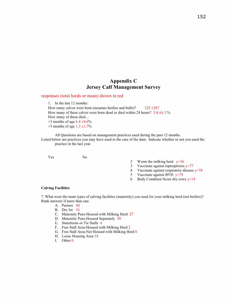
152
Appendix C Jersey Calf Management Survey
responses (total herds or mean) shown in red 1. In the last 12 months: How many calves were born (assumes heifers and bulls)? 225 ±287 How many of these calves were born dead or died within 24 hours? 5.0 ±6.3 % How many of these died.... <3 months of age 6.4 ±8.6% >3 months of age 1.3 ±1.7%
All Questions are based on management practices used during the past 12 months. Listed below are practices you may have used in the care of the dam. Indicate whether or not you used the
practice in the last year.
Yes No
2 Worm the milking herd y=36 3 Vaccinate against leptospirosis y=77 4 Vaccinate against respiratory disease y=78 5 Vaccinate against BVD y=79 6 Body Condition Score dry cows y=14
Calving Facilities 7. What were the main types of calving facilities (maternity) you used for your milking herd (not heifers)? Rank answers if more than one.
A. Pasture 40 B. Dry lot 10 C. Maternity Pens-Housed with Milking Herd 27 D. Maternity Pens-Housed Separately 30 E. Stanchions or Tie Stalls 4 F. Free Stall Area-Housed with Milking Herd 2 G. Free Stall Area-Not Housed with Milking Herd 0 H. Loose Housing Area 18 I. Other 0

153 8. What types of bedding did you use in the maternity area? Rank answers if more than one.
A. Straw 54 B. Hay 7 C. Sawdust-wet 11 D. Sawdust-kiln dry 16 E. None 4 F. Other 9
Colostrum Feeding 9. Did you wash the cows udder after calving? (before calf nursed or colostrum was milked)
A. Allow calf to nurse dam 10 B. Assist calf feeding from dam 2 C. Feed from open or nipple bucket or bottle (not allow calf to nurse dam) 79 D. Esophagael feeder 11 E. Other 0
10. Did you usually wash the cow’s udder after calving? (before calf nursed or colostrum was fed) A. No 22 B. Yes 66
11. When did calves first receive colostrum? (what is normal, not the exception) 3.8 ± 3.0 hours 12. How much colostrum did you normally feed the calf at the first feeding? 2.0 ± 0.6 quarts 13. How much colostrum did you normally feed the calf in the first d of life? 3.8 ± 1.2 quarts 14. Did you use any frozen colostrum supplement for newborn calves?
A. No 30 B. Yes 58
if yes, A. Problem cases only (included pre-partum milking) 42 B. Offspring of all first calf heifers 12 C. All calves 5
15. Did you use a colostrum supplement for newborn calves?
A. Yes 24 B. No 60
16. When did you usually separate the calf from its dam?
A. At birth before nursing 65 B. Following one nursing 15 C. Following ____ d of age. 9
17. At what age did you start feeding grain (starter or other grain) to calves? 8 ±5.9 d

154 18. Did you feed forage to calves before weaning?
A. No 44 B. Yes 44 if yes, what age 11 ± 17 d
19. Did calves have access to drinking water before weaning? A. No 20 B. Yes 67 if yes, at what age did you start? 9.8 ± 14.3 d.
Other Aspects of Raising Young (Pre-Weaned calves) 20. What are the major types of pre-weaned calf raising facilitity(s) that you used in the winter and the summer of last year? (Check appropriate ones) Rank answers if more than one. Winter Summer Hutches (individual) 45 41 Group pens (outdoors) 0 0 Group pens (indoors, in dairy barns) 6 5 Group pens (outdoors, in separate barns) 6 5 Elevated stalls – wood (in dairy barns) 0 0 Elevated stalls – wood (in separate barns) 1 1 Elevated stalls – metal (in dairy barns) 0 0 Elevated stalls – metal (in separate barns) 2 2 Individual pens (in dairy barns) 14 17 Individual pens (in separate barns) 18 22 Tied 7 8 Other 1 1 21. What are the primary types of bedding used in your calf raising facility (where applicapable)?
Rank answers A. Straw/hay 56 B. Sand 2 C. Sawdust/wood shavings 41 D. Newspaper 2 E. Corn cobbs/stalks 0 F. Other 10
22. How old are calves when you usually wean them? 9.4 ± 3.2 weeks 23. How do you decide when to wean calves? List primary criterion.
A. Size 17 B. Age 55 C. Grain intake 28 D. Other (specify) 11

155 Replacement Herd Health 24. What is the predominant disease problem with calves less than 3 months of age in your herd?
A. Digestive 63 B. Respiratory 24 C. Other (specify) 5
25. What is the source of liquid feed fed to preweaned calves?
A. Whole milk 41 B. Waste milk 25 C. Pastuerized milk 5 D. Fermented colostrum 3 E. Milk Replacer 49
26. Does the liquid diet contain any additive?
A. Antibiotics 33 B. Decox 10 C. Rumensin 2 D. Bovatec 1 E. Other (specify) 7
27. Do you feed a probiotic to preweaned calves?
A. No 58 B. Yes 29
28. Listed below are some vaccinations you might have used with your calves and heifers in the past year. For each measure, check the appropriate box. Yes No frequency before calving Brucellosis 86 IBR 75 BVD 74 PI3 74 BRSV 70 Leptospirosis 72 Virus calf scours 29 Other 33 29. Did you worm heifers during the past year?
A. No 29 B. Yes 58
30. Do you use a coccidiostat or coccidocide for coccidosis control?
A. No 10 B. Yes 78
31. If yes, what product do you use?
A. Bovatec 35 B. Corrid 14 C. Deccox 29

156
D. Other 16 Reproductive Management 32. What is your goal for age at first calving? 22.7 ± 0.5 months 33. What is the determing factor for when you decide a heifer is ready to be bred for the first time?
A. Age 22 B. Weight 11 C. Both age and weight 54 D. Other 2
34. What method of breeding heifers do you use?
A. AI only 48 B. AI first time, then bull 7 C. AI first and second time, then bull 27 D. Other (specify) 1
35. What types of bulls are used for heifers?
A. Dairy-same breed as cows? 87 B. Dairy-different breed as cows? 2 C. Beef 0
36. Did you use estrus synchronization in heifers in the past year?
A. No 50 B. Yes 36 if yes, what product did you use?
A. Prostaglandin 29 B. Synchro-mate B 3 C. Other 4
37. Do you routinely check heifers prior to breeding for reproductive infection?
A. No 76 B. Yes 11 if yes, what age 10.3 mo
38. Where did your heifers calve (check all that apply) Rank if more than one response.
A. Pasture 48 B. Dry lot 10 C. Maternity Pens-Housed with Milking Herd 26 D. Maternity Pens-Housed Separately 26 E. Stanchions or Tie Stalls 6 F. Free Stall Area-Housed with Milking Herd 0 G. Free Stall Area-Not Housed with Milking Herd 0 H. Loose Housing Area 20 I. Other 1
39. Are heifers placed in a pre-calving group prior to calving?
A. No 28 B. Yes 60

157 40. Are your first calf heifers grouped by themselves in the milking herd?
A. No 68 B. Yes 13
Do you allow first calf heifers a longer d to first breeding than older cows?
A. No 50 B. Yes 16 If yes, how much longer? 19.4 d
Milking Management and Mastitis Prevention 41. Did calves suckle each other prior to weaning?
A. No 77 B. Yes (>5%) 9
42. Did heifers have access to a pond or lagoon?
A. No 72 B. Yes 16
43. Have any heifers been milked pre-partum during the past 12 months?
A. No 47 B. Yes, what % 41, 7.9%
44. During the past twelve months, did you routinely treat heifers with antibiotics for mastitis prevention prior to calving?
A. No 66 B. Yes 20
If yes, what type of product did you use? A. Lactating 11 B. Non-Lactating product 11 How long before expected calving were heifers treated? ___weeks
Replacement Herd Culling Practices 45. What percentage of heifers were sold
A. For extra income _11.5__ % B. For beef __0.3__%
46. Which of the following most closely describes replacement culling practices in your herd?
A. No culling-all replacements raised and entered the milking herd. 38 B. Excess heifers were sold as baby calves 9 C. Excess heifers were sold as open heifers 25 D. Excess heifers were as springers 13
47. Which of the following most closely describes your milking herd size within the past twelve months. A. Increased by more than 5% 31

158
B. Decreased by more than 5% 9 C. Stayed with in +/- 5% 46
48. What was the criteria used to make heifer culling decisions.
A. Heifers ETA (Estimated Transmitting Ability) 12 B. Heifer’s Type 9 C. Dam’s performance in herd 12 D. Sire’s PTA (Predicted Transmitting Ability) 5 E. Other (specify) 15 F. No culling was done 39
Records 49. Is the herd currently enrolled in DHI’s Heifer Management Option?
A. No 46 B. Yes 30
50. What percentage of the herd is registered?
A. 0% 0 B. 1-49% 3 C. 50-99% 12 D. 100% 73
Nutrition Pre-weaned Calves 51. Feed
A. Lbs milk fed per d 6.6 ±2.0 B. Lbs milk replacer fed per d 0.96±.35 C. Lbs calf starter consumed at weaning 3.1±1.6 D. Lbs forage consumed at weaning 2.5±2.2
52.Who is primarily responsible for feeding baby cavles?
A. Owner 41 B. Spouse 28 C. Child 10 D. Herdsman 4 E. Hired help 16 F. Other 3
Other 53. Do you have a routine herd health prog with your Veterinarian?
A. No 19 B. Yes 69
if yes, frequency A. Weekly 3 B. Bi-weekly 17 C. Monthly 41 D. Other, specify 10
54. Do you have a routine vaccination program for the lactating herd?

159
A. No 10 B. Yes 77
55. Do you have a routine vaccination prog for the dry cows?
A. No 26 B. Yes 55
56. Do you work with a Nutritionist or Nutritional Consultant?
A. No 18 B. Yes 70
if yes, who provides the service A. Private consultant 21 B. Feed company 48 C. Veterinarian 7 D. Other, specify 3
57. Do you balance rations for dry cows?
A. No 34 B. Yes 50
58. Do you balance rations for dry cows in the first 60 d of their Dry Period?
A. No 35 B. Yes 47
59. Do you feed a different ration in the last 2 to 3 weeks of their dry period?
A. No 47 B. Yes 34
60. If yes, Do you have a separate ration for these cows?
A. No 52 B. Yes 33
61. Do you feed anionic salts or BioChlor or SoyChlor
A. No 49 B. Yes 32

160
Appendix D
Statistical Models
Glucose
Source DF Type III SS Mean Square F Value Pr > F
glucose0 1 2937.622641 2937.622641 6.62 0.0198
farm 1 24.005850 24.005850 0.05 0.8189
diet 3 838.918110 279.639370 0.63 0.6055
diet*farm 3 2206.010639 735.336880 1.66 0.2138
Error 17 7544.828791 443.813458
Source DF Type III SS Mean Square F Value
week 3 2198.27186 732.75729 2.63
week*glucose0 3 2317.53646 772.51215 2.77
week*farm 3 384.95233 128.31744 0.46
week*diet 9 3583.86581 398.20731 1.43
week*diet*farm 9 2337.11734 259.67970 0.93
Error(week) 51 14213.30632 278.69228
Tests of Hypotheses Using the Type III MS for trt*farm as an Error Term
Dependent Variable: glucose1
Source DF Type III SS Mean Square F Value Pr > F
diet 3 1406.452064 468.817355 0.64 0.6382
Dependent Variable: glucose2
diet 3 329.2460262 109.7486754 0.16 0.9180
Dependent Variable: glucose3
diet 3 154.7335434 51.5778478 0.94 0.5202
Dependent Variable: glucose4
diet 3 2532.352289 844.117430 24.99 0.0127
PUN
Source DF Type III SS Mean Square F Value Pr > F
pun0 1 75.6274916 75.6274916 4.28 0.0499
diet 3 140.9303684 46.9767895 2.66 0.0720
farm 1 0.1298195 0.1298195 0.01 0.9324
diet*farm 3 7.7356261 2.5785420 0.15 0.9311
Error 23 405.9680621 17.6507853
Source DF Type III SS Mean Square F Value
week 3 6.9501698 2.3167233 0.26
week*pun0 3 9.0909303 3.0303101 0.34
week*diet 9 47.7246465 5.3027385 0.59
week*farm 3 8.7471050 2.9157017 0.33
week*diet*farm 9 50.0725671 5.5636186 0.62
Error(week) 69 617.2337636 8.9454169
Tests of Hypotheses Using the Type III MS for diet*farm as an Error Term
Dependent Variable: pun1
Source DF Type III SS Mean Square F Value Pr > F

161 diet 3 72.62153644 24.20717881 10.43 0.0428
Dependent Variable: pun2
diet 3 27.46615480 9.15538493 25.89 0.0120
Dependent Variable: pun3
diet 3 51.62573050 17.20857683 38.21 0.0069
Dependent Variable: pun4
diet 3 36.94159324 12.31386441 0.76 0.5854
NEFA
Source DF Type III SS Mean Square F Value Pr > F
nefa0 1 4661.6169 4661.6169 0.22 0.6449
diet 3 813007.3868 271002.4623 12.69 <.0001
farm 1 53990.8782 53990.8782 2.53 0.1260
diet*farm 3 44020.3294 14673.4431 0.69 0.5694
Error 22 469670.3747 21348.6534
Source DF Type III SS Mean Square F Value
week 3 3405.556 1135.185 0.06
week*nefa0 3 14635.923 4878.641 0.25
week*diet 9 133538.066 14837.563 0.77
week*farm 3 15819.515 5273.172 0.27
week*diet*farm 9 88286.330 9809.592 0.51
Error(week) 66 1267557.622 19205.419
Tests of Hypotheses Using the Type III MS for diet*farm as an Error Term
Dependent Variable: nefa1
Source DF Type III SS Mean Square F Value Pr > F
diet 3 235099.0999 78366.3666 9.22 0.0504
Dependent Variable: nefa2
diet 3 277392.8637 92464.2879 10.13 0.0445
Dependent Variable: nefa3
diet 3 401210.9615 133736.9872 6.96 0.0726
Dependent Variable: nefa4
diet 3 32842.52740 10947.50913 1.51 0.3722
MR Fed, kg
Dependent Variable: kgfed kgfed
Sum of
Source DF Squares Mean Square F Value Pr > F
Diet 3 18372.10947 6124.03649 222.32 <.0001
Error 29 798.83306 27.54597
Corrected Total 32 19170.94253
Protein Fed, g
Dependent Variable: gpro gpro
Sum of
Source DF Squares Mean Square F Value Pr > F
Diet 3 45879942.65 15293314.22 511.77 <.0001
Error 29 866616.17 29883.32
Corrected Total 32 46746558.82
Fat Fed,g
Dependent Variable: gfat gfat
Sum of
Source DF Squares Mean Square F Value Pr > F

162 Diet 3 119459575.0 39819858.3 986.87 <.0001
Error 29 1170139.9 40349.7
Corrected Total 32 120629714.9
DM Fed, g
Dependent Variable: gdm gdm
Sum of
Source DF Squares Mean Square F Value Pr > F
Model 3 353127102.3 117709034.1 243.26 <.0001
Error 29 14032372.5 483874.9
Corrected Total 32 367159474.9
Gain to Feed ratio
Dependent Variable: gain_feed gain_feed
Sum of
Source DF Squares Mean Square F Value Pr > F
diet 3 0.59593017 0.19864339 18.39 <.0001
farm 1 0.00245313 0.00245313 0.23 0.6378
diet*farm 3 0.02609428 0.00869809 0.81 0.5028
Error 25 0.27001451 0.01080058
Corrected Total 32 0.95590155
BW Gained, kg
Dependent Variable: kggained kggained
Source DF Type I SS Mean Square F Value Pr > F
diet 3 440.6461490 146.8820497 45.65 <.0001
farm 1 0.8884111 0.8884111 0.28 0.6039
diet*farm 3 7.5704183 2.5234728 0.78 0.5140
Error 25 80.4404762 3.2176190
Corrected Total 32 529.5454545
Water intake, l
Dependent Variable: ctotal ctotal
Sum of
Source DF Squares Mean Square F Value Pr > F
Diet 3 386274440.0 128758146.7 2.00 0.1368
farm 1 401770950.0 401770950.0 6.24 0.0186
Error 28 1802459287 64373546
Corrected Total 32 2608168380
Average Daily Gain
Dependent Variable: ADG ADG
Sum of
Source DF Squares Mean Square F Value Pr > F
diet 3 0.46767548 0.15589183 37.98 <.0001
farm 1 0.00105171 0.00105171 0.26 0.6171
diet*farm 3 0.00965615 0.00321872 0.78 0.5140
Error 25 0.10260265 0.00410411
Corrected Total 32 0.67544063
Weekly Water Intake
Source DF Type III SS Mean Square F Value Pr > F
Diet 3 1828169.513 609389.838 1.57 0.2213
farm 1 2419121.451 2419121.451 6.24 0.0195
Diet*farm 3 1279951.992 426650.664 1.10 0.3677
Error 25 9698738.376 387949.535

163
Source DF Type III SS Mean Square F Value Pr > F
week 3 485201.96 161733.99 1.20 0.3173
week*Diet 9 877381.98 97486.89 0.72 0.6885
week*farm 3 170310.13 56770.04 0.42 0.7394
week*Diet*farm 9 975397.14 108377.46 0.80 0.6164
Error(week) 75 10146157.40 135282.10
Tests of Hypotheses Using the Type III MS for Diet*farm as an Error Term
Source DF Type III SS Mean Square F Value Pr > F
Dependent Variable: water1
Diet 3 378640.5647 126213.5216 0.73 0.5988
Dependent Variable: water2
Diet 3 1219482.594 406494.198 0.90 0.5336
Dependent Variable: water3
Diet 3 563374.3458 187791.4486 1.64 0.3478
Dependent Variable: water4
Diet 3 544053.9922 181351.3307 14.52 0.0272
Girth
Source DF Type III SS Mean Square F Value Pr > F
girth0 1 64.4585992 64.4585992 2.60 0.1206
diet 3 240.0925904 80.0308635 3.23 0.0412
farm 1 8.7063442 8.7063442 0.35 0.5593
diet*farm 3 65.1978079 21.7326026 0.88 0.4679
Error 23 570.5247699 24.8054248
Source DF Type III SS Mean Square F Value Pr > F
week 3 33.0463535 11.0154512 1.28 0.2877
week*girth0 3 30.4302981 10.1434327 1.18 0.3239
week*diet 9 65.9778807 7.3308756 0.85 0.5711
week*farm 3 9.5294439 3.1764813 0.37 0.7753
week*diet*farm 9 101.1941068 11.2437896 1.31 0.2490
Error(week) 69 593.2627710 8.5980112
Tests of Hypotheses Using the Type III MS for diet*farm as an Error Term
Source DF Type III SS Mean Square F Value Pr > F
Dependent Variable: girth1
diet 3 64.05176697 21.35058899 1.53 0.3682
Dependent Variable: girth2
diet 3 28.81792507 9.60597502 0.44 0.7403
Dependent Variable: girth3
diet 3 89.28069756 29.76023252 3.84 0.1492
Dependent Variable: girth4
diet 3 123.9200815 41.3066938 3.45 0.1681
Hip Height
Source DF Type III SS Mean Square F Value Pr > F
hip0 1 73.1119173 73.1119173 6.26 0.0196
diet 3 67.4673975 22.4891325 1.92 0.1526
farm 1 0.3149834 0.3149834 0.03 0.8710
diet*farm 3 47.6748691 15.8916230 1.36 0.2789
Error 24 280.5044069 11.6876836
Source DF Type III SS Mean Square F Value

164 week 3 7.0829711 2.3609904 1.16
week*hip0 3 6.1438113 2.0479371 1.00
week*diet 9 34.6320435 3.8480048 1.88
week*farm 3 13.3118555 4.4372852 2.17
week*diet*farm 9 26.5337368 2.9481930 1.44
Error(week) 72 147.1224912 2.0433679
Tests of Hypotheses Using the Type III MS for diet*farm as an Error Term
Source DF Type III SS Mean Square F Value Pr > F
Dependent Variable: hip1
diet 3 0.65159428 0.21719809 0.07 0.9711
Dependent Variable: hip2
diet 3 11.53035219 3.84345073 1.45 0.3827
Dependent Variable: hip3
diet 3 29.79777305 9.93259102 0.80 0.5712
Dependent Variable: hip4
diet 3 60.11972154 20.03990718 3.02 0.1941
Wither Height
Source DF Type III SS Mean Square F Value Pr > F
wither0 1 93.3443365 93.3443365 15.96 0.0005
diet 3 72.1207415 24.0402472 4.11 0.0173
farm 1 6.2705665 6.2705665 1.07 0.3107
diet*farm 3 61.7843191 20.5947730 3.52 0.0302
Error 24 140.3418896 5.8475787
Source DF Type III SS Mean Square F Value Pr > F
week 3 0.4549750 0.1516583 0.05 0.9857
week*wither0 3 0.4130819 0.1376940 0.04 0.9876
week*diet 9 59.9429368 6.6603263 2.13 0.0372
week*farm 3 14.4759707 4.8253236 1.55 0.2099
week*diet*farm 9 29.0310483 3.2256720 1.03 0.4222
Error(week) 72 224.6757344 3.1204963
Tests of Hypotheses Using the Type III MS for diet*farm as an Error Term
Source DF Type III SS Mean Square F Value Pr > F
Dependent Variable: wither1
diet 3 2.54883642 0.84961214 0.55 0.6801
Dependent Variable: wither2
diet 3 12.06290265 4.02096755 0.63 0.6411
Dependent Variable: wither3
diet 3 59.90645237 19.96881746 1.34 0.4070
Dependent Variable: wither4
diet 3 57.54548683 19.18182894 2.54 0.2317
Weekly weight
Source DF Type III SS Mean Square F Value Pr > F
wt0 1 471.7243760 471.7243760 50.47 <.0001
diet 3 627.3554946 209.1184982 22.37 <.0001
farm 1 2.0418482 2.0418482 0.22 0.6444
diet*farm 3 34.9392979 11.6464326 1.25 0.3150
Error 24 224.3128264 9.3463678
Source DF Type III SS Mean Square F Value Pr > F
week 3 5.3277254 1.7759085 1.49 0.2235
week*wt0 3 4.4762506 1.4920835 1.26 0.2963

165 week*diet 9 110.5591575 12.2843508 10.33 <.0001
week*farm 3 0.0968679 0.0322893 0.03 0.9939
week*diet*farm 9 5.3919777 0.5991086 0.50 0.8670
Error(week) 72 85.5877375 1.1887186
Tests of Hypotheses Using the Type III MS for diet*farm as an Error Term
Source DF Type III SS Mean Square F Value Pr > F
Dependent Variable: weight1
diet 3 35.57547910 11.85849303 7.08 0.0711
Dependent Variable: weight2
diet 3 119.8226893 39.9408964 6.50 0.0792
Dependent Variable: weight3
diet 3 211.1876646 70.3958882 30.71 0.0094
Dependent Variable: weight4
diet 3 371.3288190 123.7762730 37.11 0.0072
Body Length
Source DF Type III SS Mean Square F Value Pr > F
length0 1 150.5803600 150.5803600 7.19 0.0130
diet 3 158.6979582 52.8993194 2.53 0.0814
farm 1 4.3043833 4.3043833 0.21 0.6543
diet*farm 3 39.2588138 13.0862713 0.63 0.6058
Error 24 502.5121318 20.9380055
Source DF Type III SS Mean Square F Value Pr > F
week 3 4.9199939 1.6399980 0.14 0.9356
week*length0 3 4.3225925 1.4408642 0.12 0.9462
week*diet 9 43.4573442 4.8285938 0.41 0.9245
week*farm 3 32.9608454 10.9869485 0.94 0.4265
week*diet*farm 9 78.5623719 8.7291524 0.75 0.6658
Error(week) 72 842.6299186 11.7031933
Tests of Hypotheses Using the Type III MS for diet*farm as an Error Term
Source DF Type III SS Mean Square F Value Pr > F
Dependent Variable: length1
diet 3 13.81594791 4.60531597 1.07 0.4781
Dependent Variable: length2
diet 3 69.99442169 23.33147390 2.63 0.2241
Dependent Variable: length3
diet 3 43.55087116 14.51695705 1.28 0.4217
Dependent Variable: length4
diet 3 74.79406168 24.93135389 1.69 0.3389
% N retained
Sum of
Source DF Squares Mean Square F Value Pr > F
diet 3 0.12943247 0.04314416 3.74 0.0366
farm 1 0.00803656 0.00803656 0.70 0.4181
diet*farm 3 0.02727766 0.00909255 0.79 0.5206
Error 14 0.16161973 0.01154427
Corrected Total 21 0.32615540
Tests of Hypotheses Using the Type III MS for diet*farm as an Error Term
Source DF Type III SS Mean Square F Value Pr > F
diet 3 0.12943247 0.04314416 4.74 0.1166
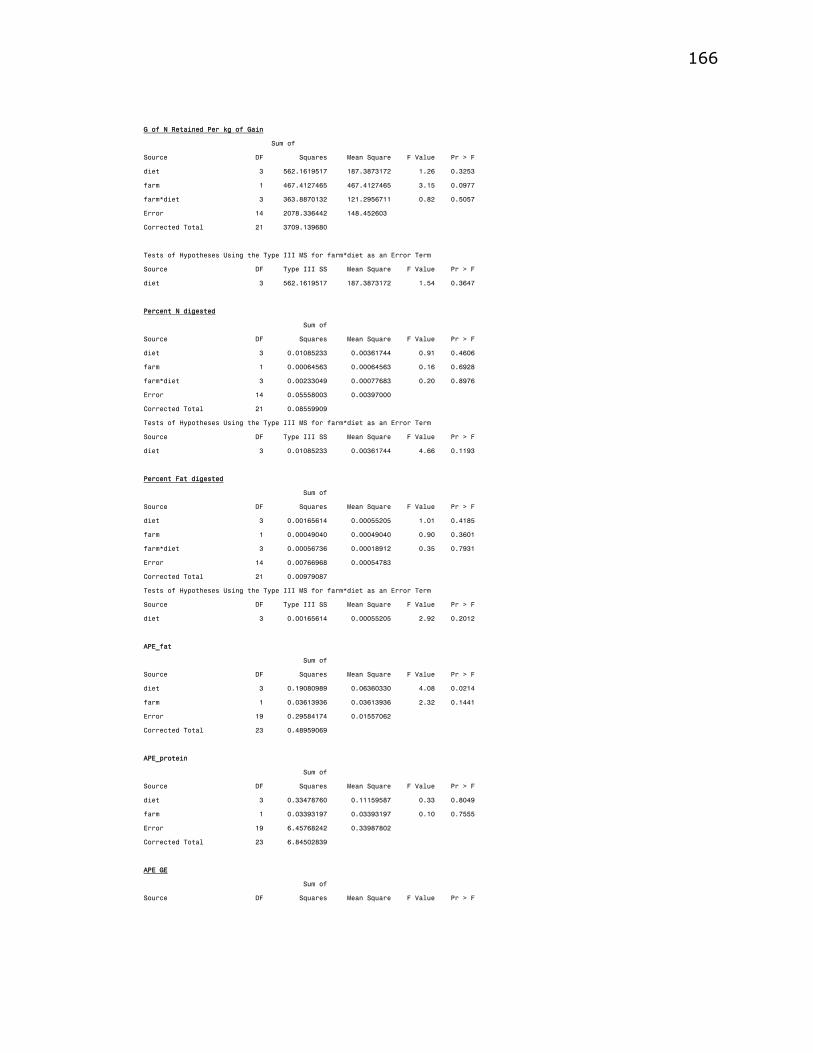
166 G of N Retained Per kg of Gain
Sum of
Source DF Squares Mean Square F Value Pr > F
diet 3 562.1619517 187.3873172 1.26 0.3253
farm 1 467.4127465 467.4127465 3.15 0.0977
farm*diet 3 363.8870132 121.2956711 0.82 0.5057
Error 14 2078.336442 148.452603
Corrected Total 21 3709.139680
Tests of Hypotheses Using the Type III MS for farm*diet as an Error Term
Source DF Type III SS Mean Square F Value Pr > F
diet 3 562.1619517 187.3873172 1.54 0.3647
Percent N digested
Sum of
Source DF Squares Mean Square F Value Pr > F
diet 3 0.01085233 0.00361744 0.91 0.4606
farm 1 0.00064563 0.00064563 0.16 0.6928
farm*diet 3 0.00233049 0.00077683 0.20 0.8976
Error 14 0.05558003 0.00397000
Corrected Total 21 0.08559909
Tests of Hypotheses Using the Type III MS for farm*diet as an Error Term
Source DF Type III SS Mean Square F Value Pr > F
diet 3 0.01085233 0.00361744 4.66 0.1193
Percent Fat digested
Sum of
Source DF Squares Mean Square F Value Pr > F
diet 3 0.00165614 0.00055205 1.01 0.4185
farm 1 0.00049040 0.00049040 0.90 0.3601
farm*diet 3 0.00056736 0.00018912 0.35 0.7931
Error 14 0.00766968 0.00054783
Corrected Total 21 0.00979087
Tests of Hypotheses Using the Type III MS for farm*diet as an Error Term
Source DF Type III SS Mean Square F Value Pr > F
diet 3 0.00165614 0.00055205 2.92 0.2012
APE_fat
Sum of
Source DF Squares Mean Square F Value Pr > F
diet 3 0.19080989 0.06360330 4.08 0.0214
farm 1 0.03613936 0.03613936 2.32 0.1441
Error 19 0.29584174 0.01557062
Corrected Total 23 0.48959069
APE_protein
Sum of
Source DF Squares Mean Square F Value Pr > F
diet 3 0.33478760 0.11159587 0.33 0.8049
farm 1 0.03393197 0.03393197 0.10 0.7555
Error 19 6.45768242 0.33987802
Corrected Total 23 6.84502839
APE GE
Sum of
Source DF Squares Mean Square F Value Pr > F
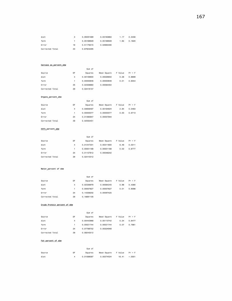
167 diet 3 0.09491589 0.03163863 1.17 0.3456
farm 1 0.05168949 0.05168949 1.92 0.1820
Error 19 0.51176315 0.02693490
Corrected Total 23 0.67923295
Carcass as_percent_ebw
Sum of
Source DF Squares Mean Square F Value Pr > F
diet 4 0.00106600 0.00026650 0.28 0.8899
farm 1 0.00000646 0.00000646 0.01 0.9354
Error 25 0.02308860 0.00092354
Corrected Total 29 0.02416157
Organs_percent_ebw
Sum of
Source DF Squares Mean Square F Value Pr > F
diet 4 0.00658497 0.00164624 2.84 0.0463
farm 1 0.00000077 0.00000077 0.00 0.9713
Error 24 0.01390647 0.00057944
Corrected Total 29 0.02050451
hhft_percent_ebw
Sum of
Source DF Squares Mean Square F Value Pr > F
diet 4 0.01247201 0.00311800 6.46 0.0011
farm 1 0.00001168 0.00001168 0.02 0.8777
Error 24 0.01157812 0.00048242
Corrected Total 29 0.02410312
Water_percent of ebw
Sum of
Source DF Squares Mean Square F Value Pr > F
diet 4 0.02336979 0.00584245 0.98 0.4380
farm 1 0.00007827 0.00007827 0.01 0.9098
Error 24 0.14338202 0.00597425
Corrected Total 29 0.16691105
Crude Protein percent of ebw
Sum of
Source DF Squares Mean Square F Value Pr > F
diet 4 0.00442968 0.00110742 0.34 0.8477
farm 1 0.00021744 0.00021744 0.07 0.7981
Error 24 0.07798752 0.00324948
Corrected Total 29 0.08243512
Fat percent of ebw
Sum of
Source DF Squares Mean Square F Value Pr > F
diet 4 0.01098097 0.00274524 18.41 <.0001
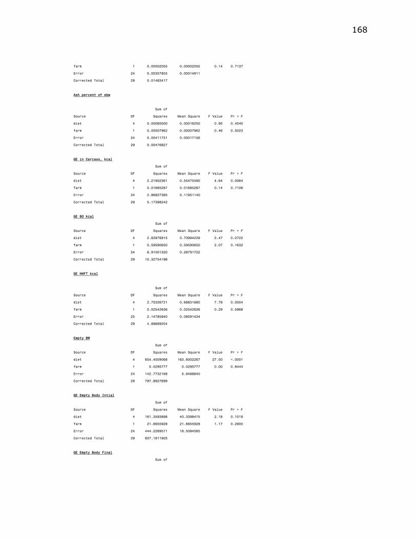
168 farm 1 0.00002055 0.00002055 0.14 0.7137
Error 24 0.00357855 0.00014911
Corrected Total 29 0.01463417
Ash percent of ebw
Sum of
Source DF Squares Mean Square F Value Pr > F
diet 4 0.00065000 0.00016250 0.95 0.4540
farm 1 0.00007962 0.00007962 0.46 0.5023
Error 24 0.00411751 0.00017156
Corrected Total 29 0.00476827
GE in Carcass, kcal
Sum of
Source DF Squares Mean Square F Value Pr > F
diet 4 2.21902361 0.55475590 4.64 0.0064
farm 1 0.01685287 0.01685287 0.14 0.7106
Error 24 2.86827365 0.11951140
Corrected Total 29 5.17398242
GE BO kcal
Sum of
Source DF Squares Mean Square F Value Pr > F
diet 4 2.83976915 0.70994229 2.47 0.0722
farm 1 0.59590650 0.59590650 2.07 0.1632
Error 24 6.91001320 0.28791722
Corrected Total 29 10.32754196
GE HHFT kcal
Sum of
Source DF Squares Mean Square F Value Pr > F
diet 4 2.75326721 0.68831680 7.78 0.0004
farm 1 0.02542636 0.02542636 0.29 0.5968
Error 25 2.14785840 0.08591434
Corrected Total 29 4.88689204
Empty BW
Sum of
Source DF Squares Mean Square F Value Pr > F
diet 4 654.4009068 163.6002267 27.50 <.0001
farm 1 0.0295777 0.0295777 0.00 0.9444
Error 24 142.7732168 5.9488840
Corrected Total 29 797.8927699
GE Empty Body Intial
Sum of
Source DF Squares Mean Square F Value Pr > F
diet 4 161.3593898 40.3398475 2.18 0.1019
farm 1 21.6655928 21.6655928 1.17 0.2900
Error 24 444.2269571 18.5094565
Corrected Total 29 607.1811905
GE Empty Body Final
Sum of

169 Source DF Squares Mean Square F Value Pr > F
diet 3 1446.593852 482.197951 1.94 0.1569
farm 1 382.959773 382.959773 1.54 0.2292
Error 19 4714.345305 248.123437
Corrected Total 23 6367.276491
GE gained
Sum of
Source DF Squares Mean Square F Value Pr > F
diet 3 1236.808122 412.269374 1.97 0.1524
farm 1 357.902757 357.902757 1.71 0.2064
Error 19 3972.548309 209.081490
Corrected Total 23 5341.288890
Fat gained
Sum of
Source DF Squares Mean Square F Value Pr > F
diet 3 14.02449501 4.67483167 21.10 <.0001
farm 1 0.53411349 0.53411349 2.41 0.1370
Error 19 4.21052343 0.22160650
Corrected Total 23 18.56350866
Ash gained
Sum of
Source DF Squares Mean Square F Value Pr > F
diet 3 0.07833784 0.02611261 0.12 0.9458
farm 1 0.00656494 0.00656494 0.03 0.8626
Error 19 4.05480157 0.21341061
Corrected Total 23 4.13512682
Water gained
Sum of
Source DF Squares Mean Square F Value Pr > F
diet 3 53.28404987 17.76134996 1.93 0.1585
farm 1 20.45738404 20.45738404 2.23 0.1521
Error 19 174.5910388 9.1890020
Corrected Total 23 279.7582604
Protein gained
Sum of
Source DF Squares Mean Square F Value Pr > F
diet 3 6.61733924 2.20577975 0.50 0.6897
farm 1 1.07725707 1.07725707 0.24 0.6284
Error 19 84.57898621 4.45152559
Corrected Total 23 91.26102017
Weekly Average Fecal Score
Source DF Type III SS Mean Square F Value Pr > F
Diet 3 1.25811073 0.41937024 2.25 0.1071
farm 1 0.17390773 0.17390773 0.93 0.3431
Diet*farm 3 0.84602909 0.28200970 1.51 0.2352
Error 25 4.65607264 0.18624291
Source DF Type III SS Mean Square F Value Pr > F
week 3 9.61244872 3.20414957 15.87 <.0001
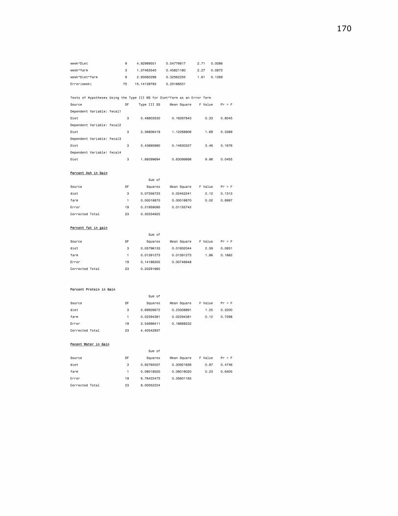
170 week*Diet 9 4.92989551 0.54776617 2.71 0.0086
week*farm 3 1.37463540 0.45821180 2.27 0.0873
week*Diet*farm 9 2.93060298 0.32562255 1.61 0.1269
Error(week) 75 15.14139793 0.20188531
Tests of Hypotheses Using the Type III MS for Diet*farm as an Error Term
Source DF Type III SS Mean Square F Value Pr > F
Dependent Variable: fecal1
Diet 3 0.48803530 0.16267843 0.33 0.8045
Dependent Variable: fecal2
Diet 3 3.36806419 1.12268806 1.69 0.3389
Dependent Variable: fecal3
Diet 3 0.43890980 0.14630327 3.46 0.1676
Dependent Variable: fecal4
Diet 3 1.89299694 0.63099898 9.96 0.0455
Percent Ash in Gain
Sum of
Source DF Squares Mean Square F Value Pr > F
diet 3 0.07356723 0.02452241 2.12 0.1312
farm 1 0.00018870 0.00018870 0.02 0.8997
Error 19 0.21959095 0.01155742
Corrected Total 23 0.30334925
Percent fat in gain
Sum of
Source DF Squares Mean Square F Value Pr > F
diet 3 0.05796133 0.01932044 2.59 0.0831
farm 1 0.01391273 0.01391273 1.86 0.1882
Error 19 0.14186305 0.00746648
Corrected Total 23 0.20291665
Percent Protein in Gain
Sum of
Source DF Squares Mean Square F Value Pr > F
diet 3 0.69926672 0.23308891 1.25 0.3200
farm 1 0.02294381 0.02294381 0.12 0.7298
Error 19 3.54696411 0.18668232
Corrected Total 23 4.40542937
Pecent Water in Gain
Sum of
Source DF Squares Mean Square F Value Pr > F
diet 3 0.92765507 0.30921836 0.87 0.4746
farm 1 0.08018020 0.08018020 0.23 0.6405
Error 19 6.76422475 0.35601183
Corrected Total 23 8.00052224

171
Appendix E
Development of a milk replacer for Jersey calves
Assumptions:
◊ Calves fed whole milk (4.7% fat, 3.5% protein) attained an ADG of 496 g/day.
This provides a realistic estimate of ADG Jersey calves on intensified diets can
obtain. Therefore, we assumed that Jersey calves fed ‘intensified’ milk replacer
programs would attain ADG of no more than 500g/day.
◊ We assumed that 28% CP in the MR is the appropriate level of protein to support
rapid growth. Recent work from lab supports this assumption (Diaz et al., 2001;
Bartlett, 2001).
◊ We also assumed that our calves were housed in an environment that was within
their thermal-neutral zone and that their maintenance energy requirement was not
influenced by environmental factors
Observations:
Refer to Table E.1
◊ The total GE intake of our calves was calculated by multiplying the total intake of
dietary fat, protein, and lactose by 9.21, 5.86, and 3.95 Mcals/g, respectively
(Brisson et al., 1957; Lister, 1971). Gross energy was multipled by 0.79 to
convert to NE (NRC 2001). This method was used to arrive at the “VPI high
estimate of NEm.”

172
◊ GE in the MR fed was also determined by bomb calorimetry. Gross energy was
multiplied by 0.79 to convert to NE (NRC 2001). This method was used to arrive
at the “VPI low estimate of NEm.”
◊ The Dairy NRC (2000) equations for NEm and NEg were applied to our data to
estimate total energy intake of our calves. However, the total intake of NE of our
calves exceeded the NRC estimate of NEm + NEg indicating that Jersey calves
have a greater requirement for NE than estimated by NRC. This is further
explained when we compare the target ADG of 650 g with the actual gains of the
calves. Our calves were fed for a target ADG of 650 g but calves fed milk,
29/16, and 27/33 had observed ADG of 457, 368, 357 g, respectively..
◊ We made the assumption Jersey calves had a much higher requirement for
maintenance energy than reported by NRC but we assumed the equation adopted
by NRC (i.e. Toullec equation) is accurate for Jersey calves. The NEm equation
used by NRC assumes that calves require 0.100 Mcal/kg of metabolic body
weight.
◊ We ‘back calculated’ to determine the maintenance energy requirement in Jersey
calves using the following equation: (equation 1) NEintake – NEm + NEg = 0.
The Toullec equation was used to calculate NEg and NEg and Neintake were
used to estimate NEm. Then the following equation (equation 2) NEm = A *
BW.75 was solved by adjusting the value of A until the average of for all calves
on our trial equaled = Neintake – NEm + Neg = 0. We determined that A= 0.139
for the “VPI high estimate of NEm” and A= 0.121 for the “VPI low estimate of
NEm.” Our new equation for maintenance energy: VPI High NEm = .139 *

173
BW.75 and VPI Low NEm = 0.121 * BW.75 . Therefore, we estimate Jersey
calves require 21 to 39% more energy for maintenance than indicated by NRC.
Development of a ‘Jersey’ Milk Replacer
Nutrient densities
◊ We assumed the following nutrient densities for GE energy in milk replacer:
3.95, 5.86, and 9.21 per g of lactose, protein, and fat, respectively. Gross Energy
was converted to NE using the following formula: NE = .79 * GE
◊ We set CP to 28% based on work by Diaz (2001) and Bartlett (2001).
1. Lactose was calculated with the following equation: lactose=100-(CP +
Fat), we ignored ash in our calculations for simplicity.
Calf parameters
◊ Used a ‘model’ Jersey with the following assumptions
30 kg of weight.
Target ADG of 500 g.
Environmental factors were in it’s thermal neutral zone.
Model
◊ Calf values were entered into Toullec equation and in the VPI NEm equation.
◊ Back calculated to get adequate fat level in milk replacer to support 500g ADG,
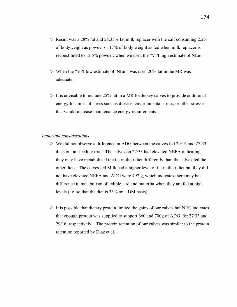
174
◊ Result was a 28% fat and 25.35% fat milk replacer with the calf consuming 2.2%
of bodyweight as powder or 17% of body weight as fed when milk replacer is
reconstituted to 12.5% powder, when we used the “VPI high estimate of NEm”
◊ When the “VPI low estimate of NEm” was used 20% fat in the MR was
adequate.
◊ It is advisable to include 25% fat in a MR for Jersey calves to provide additional
energy for times of stress such as disease, environmental stress, or other stresses
that would increase maintenance energy requirements.
Important considerations
◊ We did not observe a difference in ADG between the calves fed 29/16 and 27/33
diets on our feeding trial. The calves on 27/33 had elevated NEFA indicating
they may have metabolized the fat in their diet differently than the calves fed the
other diets. The calves fed Milk had a higher level of fat in their diet but they did
not have elevated NEFA and ADG were 497 g, which indicates there may be a
difference in metabolism of edible lard and butterfat when they are fed at high
levels (i.e. so that the diet is 33% on a DM basis).
◊ It is possible that dietary protein limited the gains of our calves but NRC indicates
that enough protein was supplied to support 660 and 700g of ADG for 27/33 and
29/16, respectively. The protein retention of our calves was similar to the protein
retention reported by Diaz et al.

175
◊ Our assumption of high NEm requirements for Jersey is calculated very
indirectly. Measuring fasting heat production of these calves would provide a
much more accurate indication of maintenance requirements.
Retained Protein
-100
-50
0
50
100
150
200
250
300
Calf
Ret
ain
Prot
ein,
g/d
ay
ObservedDiaz
Figure E.1. Protein retention of Jersey calves. Comparison of the actual protein
retention and the predicted protein retention using the Diaz equation.
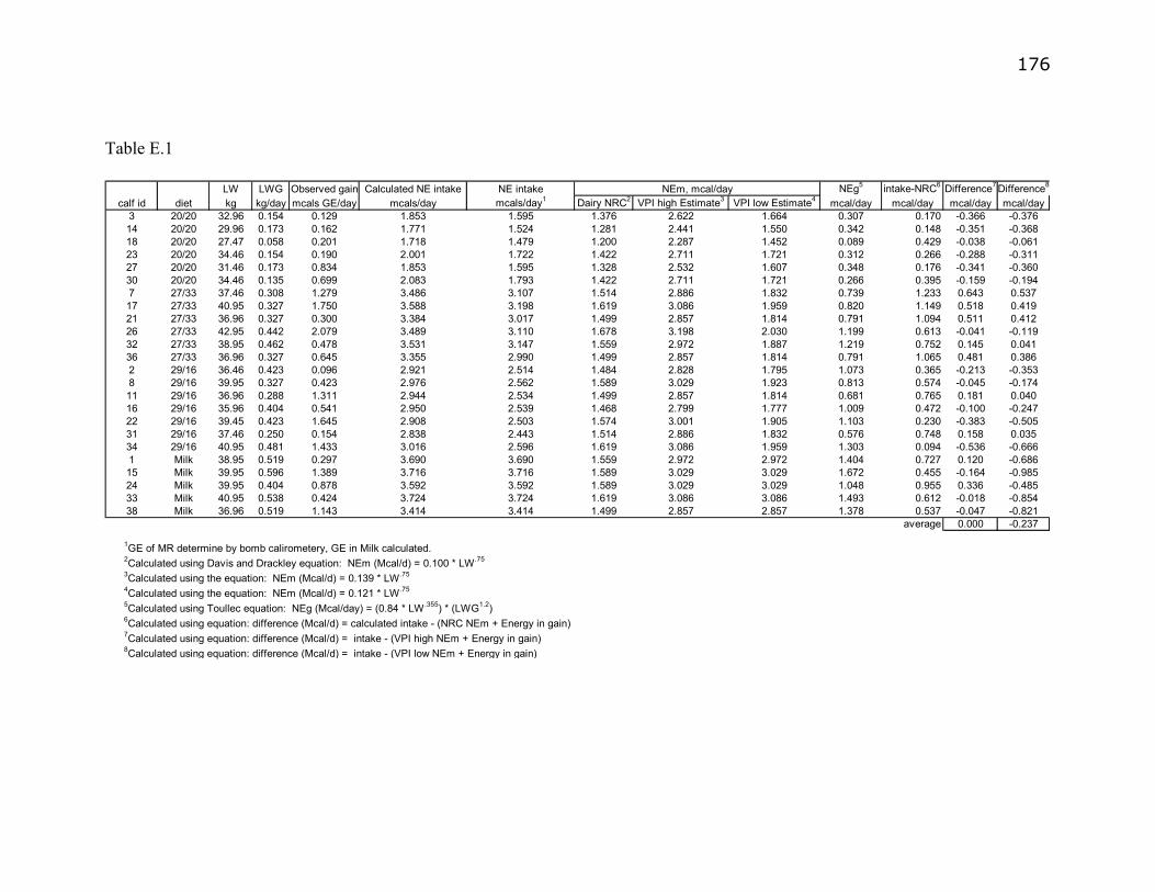
176 Table E.1
LW LWG Observed gain Calculated NE intake NE intake NEg5 intake-NRC6 Difference7 Difference8
calf id diet kg kg/day mcals GE/day mcals/day mcals/day1 Dairy NRC2 VPI high Estimate3 VPI low Estimate4 mcal/day mcal/day mcal/day mcal/day3 20/20 32.96 0.154 0.129 1.853 1.595 1.376 2.622 1.664 0.307 0.170 -0.366 -0.37614 20/20 29.96 0.173 0.162 1.771 1.524 1.281 2.441 1.550 0.342 0.148 -0.351 -0.36818 20/20 27.47 0.058 0.201 1.718 1.479 1.200 2.287 1.452 0.089 0.429 -0.038 -0.06123 20/20 34.46 0.154 0.190 2.001 1.722 1.422 2.711 1.721 0.312 0.266 -0.288 -0.31127 20/20 31.46 0.173 0.834 1.853 1.595 1.328 2.532 1.607 0.348 0.176 -0.341 -0.36030 20/20 34.46 0.135 0.699 2.083 1.793 1.422 2.711 1.721 0.266 0.395 -0.159 -0.1947 27/33 37.46 0.308 1.279 3.486 3.107 1.514 2.886 1.832 0.739 1.233 0.643 0.53717 27/33 40.95 0.327 1.750 3.588 3.198 1.619 3.086 1.959 0.820 1.149 0.518 0.41921 27/33 36.96 0.327 0.300 3.384 3.017 1.499 2.857 1.814 0.791 1.094 0.511 0.41226 27/33 42.95 0.442 2.079 3.489 3.110 1.678 3.198 2.030 1.199 0.613 -0.041 -0.11932 27/33 38.95 0.462 0.478 3.531 3.147 1.559 2.972 1.887 1.219 0.752 0.145 0.04136 27/33 36.96 0.327 0.645 3.355 2.990 1.499 2.857 1.814 0.791 1.065 0.481 0.3862 29/16 36.46 0.423 0.096 2.921 2.514 1.484 2.828 1.795 1.073 0.365 -0.213 -0.3538 29/16 39.95 0.327 0.423 2.976 2.562 1.589 3.029 1.923 0.813 0.574 -0.045 -0.17411 29/16 36.96 0.288 1.311 2.944 2.534 1.499 2.857 1.814 0.681 0.765 0.181 0.04016 29/16 35.96 0.404 0.541 2.950 2.539 1.468 2.799 1.777 1.009 0.472 -0.100 -0.24722 29/16 39.45 0.423 1.645 2.908 2.503 1.574 3.001 1.905 1.103 0.230 -0.383 -0.50531 29/16 37.46 0.250 0.154 2.838 2.443 1.514 2.886 1.832 0.576 0.748 0.158 0.03534 29/16 40.95 0.481 1.433 3.016 2.596 1.619 3.086 1.959 1.303 0.094 -0.536 -0.6661 Milk 38.95 0.519 0.297 3.690 3.690 1.559 2.972 2.972 1.404 0.727 0.120 -0.68615 Milk 39.95 0.596 1.389 3.716 3.716 1.589 3.029 3.029 1.672 0.455 -0.164 -0.98524 Milk 39.95 0.404 0.878 3.592 3.592 1.589 3.029 3.029 1.048 0.955 0.336 -0.48533 Milk 40.95 0.538 0.424 3.724 3.724 1.619 3.086 3.086 1.493 0.612 -0.018 -0.85438 Milk 36.96 0.519 1.143 3.414 3.414 1.499 2.857 2.857 1.378 0.537 -0.047 -0.821
average 0.000 -0.237
NEm, mcal/day
1GE of MR determine by bomb calirometery, GE in Milk calculated.2Calculated using Davis and Drackley equation: NEm (Mcal/d) = 0.100 * LW.75
3Calculated using the equation: NEm (Mcal/d) = 0.139 * LW.75
4Calculated using the equation: NEm (Mcal/d) = 0.121 * LW.75
5Calculated using Toullec equation: NEg (Mcal/day) = (0.84 * LW.355) * (LWG1.2) 6Calculated using equation: difference (Mcal/d) = calculated intake - (NRC NEm + Energy in gain)7Calculated using equation: difference (Mcal/d) = intake - (VPI high NEm + Energy in gain)8Calculated using equation: difference (Mcal/d) = intake - (VPI low NEm + Energy in gain)

177
Vita
Name:
Scott Shelton Bascom
Birthplace:
Springfield, Vermont – April 17, 1971
Education:
Virginia Polytechnic Institute and State University
Blacksburg, VA
Bachelor of Science 1988-1992
Major in Dairy Science
University of New Hampshire
Durham, NH
Master of Science 1994-1996
Major in Animal and Nutritional Sciences
Professional Organizations:
American Animal Science Association
American Dairy Science Association
American Jersey Cattle Association
Dairy Shrine
Virginia Tech Dairy Science Alumni Association

178


