Magnetic Targeted Drug Delivery

By

Jeffrey H. Leach

Thesis submitted to the Faculty of the

Virginia Polytechnic Institute and State University

in partial fulfillment of the requirements for the degree of

Master of Science

In

Electrical Engineering

Dr. Richard Claus, Chairman

Dr. Bradley Davis

Dr. Robert Hendricks

February 2003

Blacksburg, VA

Keywords: nanomagnetism, targeted drug delivery, magnetic microspheres,

magnetic stereotaxis system

Supported by Air Force Grant number #F49620-01-1-0407

Copyright 2003, Jeffrey H. Leach

Magnetic Targeted Drug Delivery

By

Jeffrey H. Leach

Abstract

Methods of guiding magnetic particles in a controlled fashion through the arterial system

in vivo using external magnetic fields are explored. Included are discussions of

applications, magnetic field properties needed to allow guiding based on particle

characteristics, hemodynamic forces, the uniformity of field and gradients, variable tissue

characteristics, and imaging techniques employed to view these particles while in

transport. These factors influence the type of magnetic guidance system that is needed

for an effective drug delivery system.

This thesis reviews past magnetic drug delivery work, variables, and concepts that needed

to be understood for the development of an in vivo magnetic drug delivery system. The

results of this thesis are the concise study and review of present methods for guided

magnetic particles, aggregate theoretical work to allow proper hypotheses and

extrapolations to be made, and experimental applications of these hypotheses to a

working magnetic guidance system. The design and characterization of a magnetic

guidance system was discussed and built. The restraint for this system that balanced

multiple competing variables was primarily an active volume of 0.64 cm3, a workspace

clearance of at least an inch on every side, a field of 0.3T, and a local axial gradient of 13

T/m. 3D electromagnetic finite element analysis modeling was performed and compared

with experimental results. Drug delivery vehicles, a series of magnetic seeds, were

successfully characterized using a vibrating sample magnetometer. Next, the magnetic

seed was investigated under various flow conditions in vitro to analyze the effectiveness

of the drug delivery system. Finally, the drug delivery system was successfully

demonstrated under limiting assumptions of a specific magnetic field and gradient, seed

material, a low fluid flow, and a small volume.

iii

Acknowledgments

I wish to acknowledge at Virginia Tech the support of my friends and co-workers at the

Fiber and Electro-Optic Research Center, the Optical Sciences and Engineering Research

Center, and Dr. Judy Riffle’s group. The professors and researchers at this school have

always made the time to answer questions and work through problems together. I am

honored to have worked with such bold and intellectual people. I specifically wish to

thank my advisor, Dr. Richard O. Claus, for his endless support in my research and life at

Virginia Tech. I also would like to show my appreciation to Stereotaxis, Inc. and their

staff, specifically Dr. Rogers Ritter and Dr. Duke Creighton. The Cleveland Clinic staff

has also been very receptive and I would like to particularly thank Dr. Urs Hafeli for his

support there. In addition I could have not done this without the continued love of God,

friends, and family.

iv

Table of Contents Chapter 1: Overview....................................................................................... 1

1.1 Introduction......................................................................................................... 1

1.2 Background and Motivation ............................................................................... 1

Chapter 2: Past Design Strategies................................................................... 8 2.1 Introduction......................................................................................................... 8

2.2 Stereotaxis, Inc.’s Delivery Strategy ................................................................ 21

2.3 FeRx Inc.’s Delivery Strategy........................................................................... 23

Chapter 3: Modeling ..................................................................................... 26 3.1 Blood Properties................................................................................................ 26

3.2 Hemodynamic Flow Conditions ....................................................................... 28

3.3 Comparison of Hemodynamic Forces with Magnetic Forces........................... 29

3.4 Other Mechanical Effects ................................................................................. 36

Chapter 4: Experimental ............................................................................... 39 4.1 Design and Construction of a Magnetic Microsphere Guidance System ......... 39

4.2 Characterization of Field and Gradient............................................................. 45

4.3 Characterization of Magnetic Microspheres..................................................... 57

4.4 Characterization of Microspheres Under Flow Conditions .............................. 61

Chapter 5: Conclusion .................................................................................. 71 Chapter 6: Future Work ................................................................................ 72 Appendix A: Magnetic Variables in CGI and SI Units ................................ 75 Vita................................................................................................................ 76

v

List of Figures

Figure 1. Example of a magnetic field distribution. .......................................................... 3

Figure 2. Preservation of single domains.......................................................................... 7

Figure 3. Stereotaxis’s TELSTAR Multi-Purpose Investigational Workstation ............ 22

Figure 4. Next Generation of MSS being developed by Stereotaxis, Inc104 ................... 23

Figure 5. Permanent Magnet and application of magnet used by FeRx ......................... 24

Figure 6. Blood viscosity for men and women with a +/- one standard deviation ......... 27

Figure 7. Comparison of plug vs parabolic flow of blood in large and small vessels,

respectively. .............................................................................................................. 28

Figure 8. Blood flow in a human carotid artery. ............................................................ 28

Figure 9. Magnetic and hemodynamic drag forces as a function of particle radius ....... 35

Figure 10. 6-coil super-conducting MSS built by Wang NMR, Inc................................ 37

Figure 11. Calculated field and gradients along the axis for (a) x or y-axis coil, and (b) z-

axis coil for 6-coil superconducting system. The arrows indicate the edge of a 20-cm

diameter spherecentered in the region where a head can be located. ...................... 38

Figure 12. Variable magnetic field and gradient test system........................................... 40

Figure 13. Wiesel Powerline WM60 Actuator. The actuator consists of a sliding

carriage(1), scraper brushes(2), tubular section with sliding bars(3), ball screw(4),

guideway for screw supports(5), guideways(6), covering strip(7), ball-bearing

guided carriage(8), ball nut unit(10), bearing housing and fixed bearing(11).......... 41

Figure 14. Diagram of Goldline XT MT(B)304 Motor. .................................................. 42

Figure 15. Servostar brushless servo amplifier with integrated power supply. ................ 43

Figure 16. Kollmorgen’s Servostar Motionlink software. ............................................... 43

Figure 17. Various grades of NdFeB. ............................................................................... 44

Figure 18. The THM 7025 3-Axis Hall Teslameter ........................................................ 45

Figure 19. Side view of the right field magnet and the corresponding traces made in Z-Y

plane.......................................................................................................................... 46

Figure 20. Theoretical field strengths predicted using ANSOFT’s 3D Maxwell Equation

Finite Element Analysis Software compared to measured values. ........................... 47

Figure 21. Total X-Component of B Field....................................................................... 48

vi

Figure 22. Total Y-Component of B Field........................................................................ 49

Figure 23. Total Z-Component of B Field. ....................................................................... 50

Figure 24. Total X-Component Gradient of B Field......................................................... 51

Figure 25. Total Y-Component Gradient of B Field......................................................... 52

Figure 26. Total Z-Component Gradient of B Field. ........................................................ 53

Figure 27. Total X-Component Gradient of B Field * X-Component of B Field. ........... 54

Figure 28. Total Y-Component Gradient of B Field * Y-Component of B Field. ........... 55

Figure 29. Total Z-Component Gradient of B Field * Z-Component of B Field. ............ 56

Figure 30. Composite View. From left to right: (a)Magnitude of Field in the x-plane, y-

plane, and z-plane. (b) Gradient in the x-plane, y-plane, and z-plane. (c) Field-

Gradient product in the x-plane, y-plane and z-plane............................................... 57

Figure 31. The LakeShore 7300 Vibrating Sample Magnetometer. ................................. 58

Figure 32. Flowchart of VSM operations. ....................................................................... 59

Figure 33. VSM Characterization of Dynabeads Product Number 142.04. .................... 60

Figure 34. VSM Characterization of Multi-Domain Samarium-Iron-Nitride. ................ 61

Figure 35. Manipulation of a ferrofluid with electromagnets (Arrows depict current

direction). .................................................................................................................. 62

Figure 36. Experimental setup for load testing of microspheres. ..................................... 63

Figure 37. Suspended solution of Dynabeads product 142.04 under static flow conditions.

................................................................................................................................... 63

Figure 38. Suspended solution of Dynabeads product 142.04 under dynamic flow

conditions.................................................................................................................. 64

Figure 39. Suspended solution of Dynabead’s product 142.04 under variable

static/dynamic flow conditions. ................................................................................ 65

Figure 40. Suspended solution of Dynabead’s product 142.04 under dynamic flow

conditions with higher field-gradient, smaller tubing size, and slower flow

conditions.................................................................................................................. 66

Figure 41. Characteristic 281 micron MnZn sample. ....................................................... 67

Figure 42. VSM Characterization of MnZn...................................................................... 67

Figure 43. Suspended solution of MnZn under dynamic flow conditions with higher

field-gradient, smaller tubing size, and slower flow conditions. .............................. 68

vii

Figure 44. (a.) Suspended solution of MnZn (b.) Outer field magnets moved 1 inch

away from the center field magnet, unsuspending particles (c.) Outer field magnets

moved 1 inch inward and along direction of tubing to resuspend particles.............. 69

Figure 45. Zoom 160 Optical System modified with non-ferric components capable of

micrometer resolution within the magnetic workspace. ........................................... 72

Figure 46. Platform grouping of microspheres. ................................................................ 73

List of Tables

Table 1. Typical B field values in selected applications., ................................................. 4

Table 2. Design and performance characteristics of selected ophthalmic magnetic

manipulation systems used since the 1950s................................................................ 9

Table 3. Design and performance characteristics of selected cardio/endovascular

magnetic manipulation systems used since the 1950s. ............................................. 11

Table 4. Design and performance characteristics of selected gastroenterology magnetic

manipulation systems used since the 1950s. magnetic manipulation systems used

since the 1950s.......................................................................................................... 13

Table 5. Design and performance characteristics of selected nonstereotactic

neurosurgical magnetic manipulation system used since the 1960s to guide catheters

or concentrate ferromagnetic slurries........................................................................ 16

Table 6. Design and performance characteristics of selected magnetic manipulation

systems used in orthopedic, urological, and pulmonary applications since the 1960s.

................................................................................................................................... 18

Table 7. Design and performance characteristics of various exploratory magnetic

manipulation systems that are either functionally stereotactic or that employ

stereotactic instrumentation in their operation.......................................................... 20

Table 8. MSS magnetic manipulation systems used to date. .......................................... 22

Table 9. Properties of N48M. ........................................................................................... 44

Table 10. Physical Characteristics of Dynabeads M-280 Magnetic Microspheres. ......... 60

1

Chapter 1: Overview

1.1 Introduction

The purpose of this thesis is to consider how externally applied magnetic fields can be

used to guide materials internal to the body. The primary concern will be to examine

current and prior attempts to discover a fusion of past designs that allow the guidance of

magnetic microspheres. It is hypothesized that control of magnetic microspheres in vivo

is feasible given a strong magnetic field and gradient space superpositioned on an arterial

system. This work is fueled by the general nanotechnology initiative and the general

desire for less invasive surgery using electromagnetic field-directed nanoparticles. The

current nanotechnology initiatives are motivated by the added functionality derived from

reducing the overall size of working systems. A general overview of the most important

variables of concern and background is presented in the first section. Next, a review of

prior and present magnetic field-based delivery systems will be explored. Modeling the

controlling variables and their interactions are described in closer detail in the third

section. Finally, in the fourth section, first-order experimental verification is performed

to ensure the accuracy of the modeling. The end discussion summarizes results and

provides recommendations for future research.

1.2 Background and Motivation

Magnetic microspheres have potential use as magnetic seeds for drug delivery. Such

microspheres are paramagnetic and have been made to range in size from approximately

one micron to greater then 600 microns. To control the motion of such microspheres

within the body, a magnetic force due to an externally applied magnetic field and a

hemodynamic drag force due to blood flow combine to create a total vector force on the

spheres. In order to effectively overcome the influence of blood flow, and in order to

achieve desired external magnetic field-controlled guidance, the magnetic force due to

the external field must be larger than the drag force.

2

To a first approximation, the magnetic force on the microsphere is governed by

( ), [Newtons]oF m B= ∇ • (1)

where F is the magnetic force, m is the total magnetic moment of the material in the

microsphere, ∇ is the gradient, assumed in our modeling to be derived from

characteristics of the B field alone, and B is the magnetic flux density, also known simply

as the B field. Each of these quantities thus influences the degree to which an external

magnetic field may be used to guide internal microspheres. The del operator, ∇, is

defined as

x y zˆ ˆ ˆa a ax y z∂ ∂ ∂

∇ ≡ + +∂ ∂ ∂

(2)1

in rectangular coordinates. It is noted that the gradient of a scalar function at any point is

the maximum spatial change of the magnetic field at any point. The B field tends to align

the net magnetic moment of the particle in a fixed direction while the gradient leads to a

force that may move the particle. An extended analysis of magnetically-induced forces

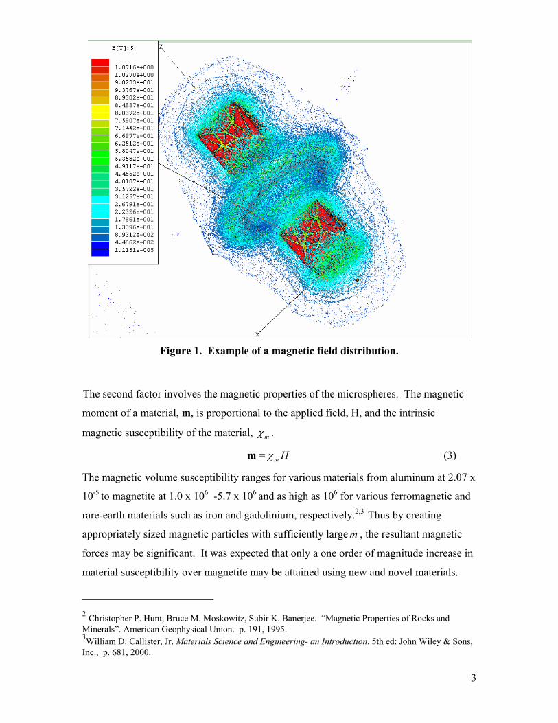
on magnetic materials is considered in Section 3.3 below. Figure 1 depicts an example

magnetic field that would act on a magnetic particle.

Similar to rolling down a steep hill, the steeper the gradient is, the more total force will

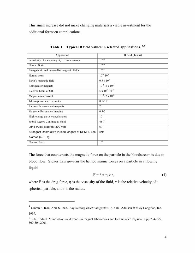
be placed on the particle. Table 1 gives typical B field values found in the universe and

gives a sense of what values are realizable for a working magnetically controlled

microsphere guidance system. Please refer to Appendix A for additional reference

information of other magnetic variables and their corresponding units. The most

challenging aspect of manipulating magnetic microspheres in vivo is the fact that the

magnetic field and gradients weaken as 1/r3, so large fields are required for human

patient-sized systems.

1 Umran S. Inan, Aziz S. Inan. Engineering Electromagnetics. p. 277. Addison Wesley Longman, Inc.

1999.

3

Figure 1. Example of a magnetic field distribution.

The second factor involves the magnetic properties of the microspheres. The magnetic

moment of a material, m, is proportional to the applied field, H, and the intrinsic

magnetic susceptibility of the material, mχ .

m = mχ H (3)

The magnetic volume susceptibility ranges for various materials from aluminum at 2.07 x

10-5 to magnetite at 1.0 x 106 -5.7 x 106 and as high as 106 for various ferromagnetic and

rare-earth materials such as iron and gadolinium, respectively.2,3 Thus by creating

appropriately sized magnetic particles with sufficiently large m , the resultant magnetic

forces may be significant. It was expected that only a one order of magnitude increase in

material susceptibility over magnetite may be attained using new and novel materials.

2 Christopher P. Hunt, Bruce M. Moskowitz, Subir K. Banerjee. “Magnetic Properties of Rocks and Minerals”. American Geophysical Union. p. 191, 1995. 3William D. Callister, Jr. Materials Science and Engineering- an Introduction. 5th ed: John Wiley & Sons, Inc., p. 681, 2000.

4

This small increase did not make changing materials a viable investment for the

additional foreseen complications.

Table 1. Typical B field values in selected applications. 4,5

Application B field (Teslas)

Sensitivity of a scanning SQUID microscope 10-16

Human Brain 10-13

Intergalactic and interstellar magnetic fields 10-11

Human heart 10-9-10-8

Earth’s magnetic field 0.5 x 10-5

Refrigerator magnets 10-4- 8 x 10-3

Electron beam of CRT 5 x 10-4-10-3

Magnetic read switch 10-3- 2 x 10-3

1-horsepower electric motor 0.1-0.2

Rare-earth permanent magnets 2

Magnetic Resonance Imaging 0.5-5

High-energy particle accelerators 10

World Record Continuous Field 45 T

Long-Pulse Magnet (800 ms) 60

Strongest Destructive Pulsed Magnet at NHMFL-Los

Alamos (4-8 µs)

850

Neutron Stars 108

The force that counteracts the magnetic force on the particle in the bloodstream is due to

blood flow. Stokes Law governs the hemodynamic forces on a particle in a flowing

liquid.

F = 6 π η v r, (4)

where F is the drag force, η is the viscosity of the fluid, v is the relative velocity of a

spherical particle, and r is the radius.

4 Umran S. Inan, Aziz S. Inan. Engineering Electromagnetics. p. 448. Addison Wesley Longman, Inc.

1999. 5 Fritz Herlach. “Innovations and trends in magnet laboratories and techniques.” Physica B. pp.294-295, 500-504.2001.

5

Other variables of concern internal to the body are tissue porosity to microspheres of

certain size (and resulting m ), and allowable cell damage caused by incompatible

microsphere sizes and forces. A highly porous tissue allows small microspheres to be

easily manipulated out of the bloodstream and into the tissue. However, a relatively tight

tissue structure would require more magnetic field-induced force to pull the microspheres

out of the bloodstream and such interfacial transport could cause damage to the tissue.

Therefore, the microsphere size and forces needed for effective microsphere

manipulation are highly dependent on the area in which drug delivery is to be performed.

The motivation for this project comes from the numerous potential applications for a

magnetic field-controlled drug delivery system. Targeted microsphere delivery platforms

have the ability to deliver simultaneous medical applications of gene therapy6, destroy

built up plaque in arteries, image and extract foreign metallic and ferric objects from the

body, and affect cancer therapies of in-vitro vesicular blockage7, targeted radiation

therapy8, and hyperthermia9.

Drug targeting would allow a lower whole body dosage of medicines and treatments that

otherwise would not be a viable solution to a problem due to the toxicity of higher doses.

An example of this is Dr. Kurt Hofer’s work with hyperthermia10. Hofer was able to

make cancerous cells more susceptible to heat compared to normal cells by introducing

6C. Plank, F. Scherer, U. Schillinger, M. Anton, C. Bergemann. “Magnetofection: Enhancing and

Targeting Gene Delivery by Magnetic Force.” Fourth International Conference on the Scientific and

Clinical Applications of Magnetic Carriers. 67-70, 2002. 7 G.A. Flores and J. Liu. “In-vitro blockage of a simulated vascular system using magnetorheological

fluids as a cancer therapy.” Fourth International Conference on the Scientific and Clinical Applications of

Magnetic Carriers. 19-21, 2002. 8 Hafeli, U., Pauer, G., Failing, S., Tapolsky, G. “Radiolabeling of Magnetic Particles with Rhenium188

for Cancer Therapy”, Journal of Magnetism and Magnetic Materials. Vol. 225 p.73-78, 2001. 9 Kurt Hofer. “Hyperthermia and Cancer.” Fourth International Conference on the Scientific and Clinical

Applications of Magnetic Carriers. 78-80, 2002. 10 Kurt Hofer. “Hyperthermia and Cancer.” Fourth International Conference on the Scientific and Clinical

Applications of Magnetic Carriers. 78-80, 2002.

6

misonidazole, which takes advantage of the observation that cancerous cells use more

oxygen than normal cells. The cancerous cells absorbed misonidazole more than normal

cells, thus making the cancerous cells more susceptible to heat. When heat was applied

to the area, the cancer cells died faster then the surrounding normal cells. This was a

faster method of curing cancer compared to the routine multifraction radiotherapy. The

major problem with this treatment is that buildup in the brain of this drug causes

neuropathy 10-12 months later. Careful delivery and removal of toxins for such local site

activation could be accomplished with magnetic drug delivery.

Analysis of development of magnetically targeted drug delivery systems.

The first step in the design of such a system is to choose a seed material. For

experimental work discussed below ferromagnetic magnetite (Fe3O4) was chosen due to

its relatively high magnetic moment in reasonably sized particles and because of the

amount of work that has be done to demonstrate its relatively low toxicity in the body

when encapsulated in a protective protein cage. 11

The next design step is to incorporate this magnetic seed with different drugs.

Encapsulation of the drugs with magnetite shells or attaching the drugs to a

functionalized outer coating may be performed. Functionalized outer coatings of

microspheres are a well-established procedure.12 Such modified magnetic microspheres

may then be delivered to the target cells, where the microspheres will decompose due to

their poly-lactic acid or other degradable coating, and the drug will be delivered.

11 Linda A. Harris. “Polymer Stabilized Magnetite Nanoparticles and Poly(propylene oxide) Modified

Styrene-Dimethacrylate Networks.” Dissertation Submitted to Virginia Polytechnic Institute and State

University, April 19, 2002. 12 Tech Notes. Bang Labs, Inc. http://www.bangslabs.com/support/index.php

7

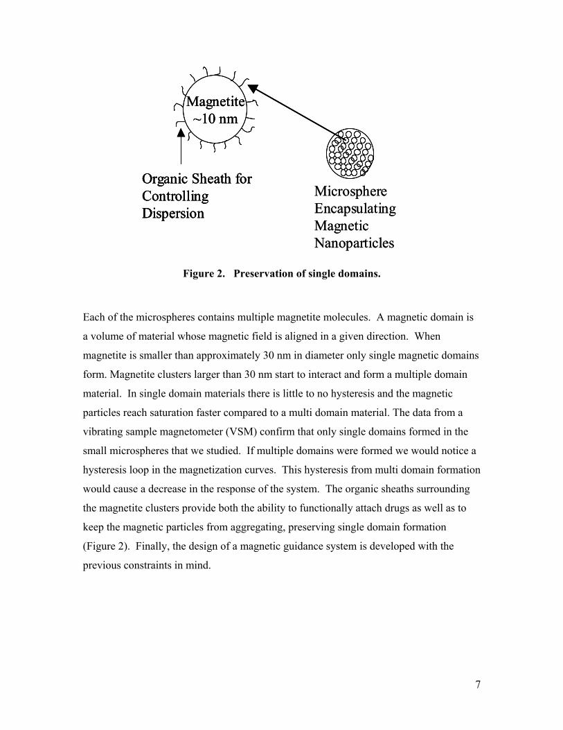
Magnetite~10 nm

Organic Sheath for Controlling Dispersion

Microsphere Encapsulating MagneticNanoparticles

Magnetite~10 nm

Organic Sheath for Controlling Dispersion

Magnetite~10 nm

Organic Sheath for Controlling Dispersion

Microsphere Encapsulating MagneticNanoparticles

Figure 2. Preservation of single domains.

Each of the microspheres contains multiple magnetite molecules. A magnetic domain is

a volume of material whose magnetic field is aligned in a given direction. When

magnetite is smaller than approximately 30 nm in diameter only single magnetic domains

form. Magnetite clusters larger than 30 nm start to interact and form a multiple domain

material. In single domain materials there is little to no hysteresis and the magnetic

particles reach saturation faster compared to a multi domain material. The data from a

vibrating sample magnetometer (VSM) confirm that only single domains formed in the

small microspheres that we studied. If multiple domains were formed we would notice a

hysteresis loop in the magnetization curves. This hysteresis from multi domain formation

would cause a decrease in the response of the system. The organic sheaths surrounding

the magnetite clusters provide both the ability to functionally attach drugs as well as to

keep the magnetic particles from aggregating, preserving single domain formation

(Figure 2). Finally, the design of a magnetic guidance system is developed with the

previous constraints in mind.

8

Chapter 2: Past Design Strategies

2.1 Introduction

There have been many attempts in the past to create platform technologies that can guide

and deliver drugs, make repairs, and essentially give one’s hands the dexterity to

seamlessly manipulate nature from macro and micro sizes to the nanometer scale. This

range of maneuverability and control over matter allows noninvasive surgery and the

ability to pass through tissue and even cell walls instead of cutting or lysing them to

obtain internal access to a material or body. D. Montgomery et al. conceived the first

multicoil superconducting magnetic manipulator in 196913. Commercially it appears that

only Stereotaxis, Inc. and FeRx Inc. are working on FDA approval for various magnetic

targeted drug delivery methods.

One large commercial area of magnetic manipulation that has been completed is in the

use of magnets to manipulate and retrieve foreign ferric objects in the eye. Examining

Table 2 we take note of the various magnet designs and their applications. Some of these

applications also include retinal tear repair and cataract emulsification.

Another extensive area that has been investigated is the use of magnetic manipulation to

perform noninvasive surgery on the cardiologic and endovascular systems. These

systems represent a significant percentage of the human body and further demonstrate the

wide range of applications that can be performed with magnetic targeting. The

experiments documented in Table 3 demonstrate angiography, stripping varicose veins,

removing plaque deposits, chemotherapy and aneurysm embolization.

13 D Montgomery, R.J. Weggel, M.J. Leupol, S.B. Yodh, and R.K. Wright. J.Appl. Phys. 40, 2129 (1969).

9

Table 2. Design and performance characteristics of selected ophthalmic magnetic

manipulation systems used since the 1950s.14

Authors Apparatus/ Method Application Design Features Results Year

M.F.McCasli

n15

Pulsed-field, high-

gradient electro-magnet

Removal of

intraocular foreign

bodies (non-specific

injuries)

50% Fe – 50% Co core,

34 cm long x 7.4 cm

diam., 120° pole-place

tip angle

Maximum

gradient = 650

T/m within 1 cm

of probe tip

1958

N.R. Bronson

II16

Storz-Atlas (S-A)

magnet, Bronson-

Magnion pulsed

magned

Comparison of

pulling force vs. tip

geometry and

temperature

Solid-state Hall-effect

transducers used to map

the tip’s field gradient

B-H magnet has

pulling force = 7x

that of S*A

magnet (@50%

duty cycle)

1968

R.J.

AmaLong17

Lancaster-Geiger

magnet, Bronson-

Magnion magnet

Removal of

intraocular foreign

bodies (shrapnel

injuries)

Hand-held magnets

used in conjunction

with cryothermic

wound closure

Foreign objects >

3mm may detach

retine unless

approached

posterioly

1970

G. Landwehr

et al. 18

Pulsed-field, hand-held

magnet, and axial inner-

pole magnet

Improved-control

method for extracting

intraocular foreign

bodies

10-ms pulse sequence

used a 50% duty cycle,

test particle mass =

0.043g

Oscillatory

relaxtion time –

100ms, object

moved in steps of

= 0.4

mm./sequence

1977

G.M.

Stephens et

al. 19

Standard ophthalmic

hand manget, curved

and straight tips

Measurement of the

distribution of

magnetic flux

surrounding tip

Magnet operated at 120

V over a current range

of 100 – 400mA

1 mg object must

be < 8mm from

magnet tip to

move in vitreous

@ 400 mA

1977

D. Lobel et

al20

Magnetically guided

intraocular sphere,

(Teflon coated)

Unfolding of

overlapped retina

followed, by repair of

retinal tear

Sphere diam. Range-

0.5 to 6.0 mm; magnet-

tipped diathermy probe

guides sphere

In vivo studies

showed no retinal

bleeding, but some

flattening and

1978

14 G.T. Gillies, R.C. Ritter, W.C. Broaddus, M.S. Grady, M.A. Howard III, R.G. McNeil. “Magnetic Manipulation Instrumentation for Medical Physics Research” Rev. Sci.Instrum. 65 (3), March 1994. 15 M F. McCaslin, Trans. Am. Ophthalmol. Sot. 56, 571 (1958). 16 N. R. Bronson II, Arch. Ophthal. 79, 22 (1968). 17 R. J. Amalong, Am. J. Ophthal. 70, 10 (1970). 18 G. Landwehr, K. Dietrich, H. Weber, W. Bushmann, and H. Neubauer,Ophthalmic Res. 9, 308 (1977). 19 G. M. Stephens, A. A. Cinotti, A. R. Caputo, E. P. Veltri, and A. A. Vigorito, in Proceedings of the San Diego Biomedical Symposium, edited by J. I. Martin (Academic, New York, 1977), Vol. 16, pp. 387-390.

10

Authors Apparatus/ Method Application Design Features Results Year

compression

D. J.

Coleman21

Bronson-Magnion

pulsed magnet with

customized tips

Comparison of

pulling force vs. tip

geometry

Tip extension improves

the access to foreign

body and minimizes

extraction damage

Coleman

“straight” tip and

Bronson “long” tip

produce B= 2,000

G at 2 cm from tip.

1982

A.

Schumann,

Inc. 22

High-field giant magnet

with conical coil and

iron core

Explosion-proof

system for removal on

intraocular foreign

bodies

Five-step power

regulating switch

thermostatic shutoff to

prevent overheating

Field strength of

1.3 T at tip, 0.5 T

at 1 cm, and 0.3 T

at 2 cm

1982

H. Weber et

al23,24

Magnetically driven

introcular oscillator

(two external coils)

Determination of the

compliance and

damping of the

vitreous

Spheres of 0.5 to 1.0

mm diam. Driven at 1

to 60 Hz by two pulsed

coils

7.6 x 104 H*m-3 =

spring constant per

unit area of in

vitro human

vitreous

1982

D.R. May et

al. 25

Modified 20-gauge tip

for Bronson intraocular

electromagnet

Extraction of foreign

bodies by insertion of

tip through pers plana

Standard Bronson acorn

tip machine down to

cyline 20-gauge diam.

X 5 mm long

Apparatus has

been used

successfully in ~

10 human-clinical

trials

1989

Aura

Systems, Inc.

26

Computer-aided, multi-

coil magnetic

manipulation

(“KELMAST”)

Cataract

emulsification via

high-speed rotation of

an implanted object

Currents in four conical

coils controlled by

surgeon via joystick

“magnabit”

inserted through 1-

mm incision;

feedback cancels

vibrational effects

1992

20 D. Lobel, J. R. Hale, and D. B. Montgomery, Am. J. Ophthalmol. 85,699 ( 1978). 21 D. J. Coleman, Am. J. Ophthalmol. 85, 256 ( 1978). 22 Schumann GM3F & GM3FEX Giant Eye Magnets” (A. Schumann,Inc., West Concord, Massachusetts, August, 1982), 4 pp. 23 H. Weber and G. Landwehr, Ophthalmic Res. 14, 326 (1982). 24 H Weber, G. Landwehr, H. Kilp, and H. Neubauer, Ophthalmic Res. 14, 335 (1982). 25 D. R. May, F. G. Noll, and R. Munoz, Arch. Ophthalmol. 107, 281(1989). 26 S. Burke, B. Laufer, E. Leibzon, A. Schwartz, M. Strugach, R. Van Allen, and C. Warren, Magnetically Assisted Cataract Surgery: Overview (Aura Systems, Inc., El Segundo, California, October 27, 1992), 2 pp.

11

Table 3. Design and performance characteristics of selected cardio/endovascular

magnetic manipulation systems used since the 1950s. 27

Authors Apparatus/ Method Application Design Features Results Year

H.

Tillander28,29,

30

Permanent-magnet-

tipped catheter guided

by electromagnet

Selective angiography

of canine

pancreaticoduodentre

nal artery

Multi-magnet catheter

tip, made of Platinax-II

cylinders, max. diam. =

2.1 mm

x-ray image

intensifier required

screening with 2

layers of 2-mm

Mumetal

1951

H.T. Modny

et al. 31

Transvenous plumb-line

navigated through the

vein by external magnet

Minimally invasive

technique used for

stripping varicose

veins

Magnetically attracted

probe mass draws

stripping cord through

the vein.

Only two incisions

needed to facilitate

entrance, exit and

guidance of cord

1958

E.H. Frei et

al. 32,33,34

Para-operational device

(“POD”), vix., magnet-

tipped catheter

Placement of

intravascular

transducers, drug

delivery and biopsy

Permanent magnet tip ~

1 mm diam. X 5 mm

long with soft rubber

sheath as cover

Several different

versions of device

built and used in

human clinical

trials

1963

S.B. Yodh et

al. 35

Catheter guidance via

two goniometer-

mounted 2.5 kW

electromagnets

Delivery of contrast

agents, chemotherapy,

aneurysm

embolization

Pt-Co magnet-tips, 1.3

mm diam., with heat-

soluble paraffin link to

catheter

> 90° turn-angle

achieved during in

vivo study in

rabbit renal-vein

system

1968

J. A. Taren

and T.O.

Gabrielsen36,

37

Transvascular magnetic

electrode catheter, ac-dc

guide magnet

RF-lesioning of extra-

cranial arteriovenous

malformations

(humans)

Sm-Co magnet, .5 mm

diam. X 1.5 mm long

on coiled electrode

inside catheter

Guidance range ~

12 cm, 3-mm

thrombi produced

via RF heating of

catheter tip

1970

27 G.T. Gillies, R.C. Ritter, W.C. Broaddus, M.S. Grady, M.A. Howard III, R.G. McNeil. “Magnetic Manipulation Instrumentation for Medical Physics Research” Rev. Sci.Instrum. 65 (3), March 1994. 28H. Tillander, Acta Radiol. 35, 62 (1951). 29 H. Tillander, Acta Radiol. 45, 21 (1956). 30 H. Tillander, IEEE Trans. Magn. MAC-4 355 (1970). 31 M. T. Modny, G. Ridge, and J. P. Bambara, U.S. Patent No. 2 863 458 (9 December 1958). 32 E. H. Frei, S. H. Leibinsohn, H. N. Heufeld, and H. N. Askenasy, in Proceedings.of the 16th Annual Conference on Engineering in Medicine and Biology, edited by D. A. Robinson (Harry S. Scott, Inc., Baltimore, MD, 1963), Vol. 5, pp. 156-157. 33 E. H. Frei, J. Driller, H. N. Neufeld, I. Barr, L. Bleiden, and H. M. Askenasy, Med. Res. Eng. 5, 11 (1966). 34 ME. H. Frei and S. Leibmsohn, U.S. Patent No. 3 358 676 (19 December 1967). 35 B. Yodh, N. T. Pierce, R. J. Weggel, and D. B. Montgomery, Med. Biol. Eng. 6, 143 (1968). 36 J. A. Taren and T. 0. Gabrielsen, Science 168, 138 ( 1970).

12

Authors Apparatus/ Method Application Design Features Results Year

J.H.

Sobiepanek38

Magnetically-guided

catheter with cibrating

plunger in tip

Percussive destruction

of blockages in the

coronary arteries

Externally-applied,

pulsed magnetic field

causes the plunger to

reciprocate

Design studies

showed that

probes 2.3 mm

diam x 15 mm

long were feasible

1970

D.B.

Montgomery

et al. 39

Catheter guidance via

one goniometer-

mounted 2.5 kw

electromagnet

Catherization of

internal carotid artery

and its divisions

0.5 mm SilasticTM

catheter with 0.9 mm

diam. Pt-Co tip

monitored by

fluroscope

Catheter has

reached the

anterior

communicating

junction oin four

human trials

1970

D.H.

Ledermen et

al. 40

Intravascular magnetic

suspension of test

objects in pulsatile flow

In vivo assessment of

hemocompatbiliity of

prosthetic materials

Test device ~ 5 mm

diam x 50 mm long;

Hall probes sense test

device position

Feasibility of non-

contact suspension

demonstrated in

canine aorta (in

vivo)

1977

W. Ram and

H. Meyer41

Permanent-magnet

tipped polyurethane

angiography catheter

Intraventricular

catheteriation in heart

of neonate

1.2 mm diam x 8 mm

long magnetic tip in

4.7F catheter; x-ray

visualization

Catheter steerable

up to 40 mm from

external magnet,

no complications

during use

1991

Further, gastro-intestinal track magnetic manipulation, such as the prior work indicated in

Table 4, demonstrates the feasibility of guidance under different flow conditions and size

restrictions. Demonstrated applications include resolving intestinal obstructions, tissue

biopsies, increased visualization with magnetic contrasts, and repositioning of tissue for

radiation treatment.

37 J. A. Taren and T. 0. Gabrielsen, IEEE Trans. Magn. MAC-C, 358 (1970). 38 J. M. Sobiepanek, IEEE Trans. Magn. MAC-6, 361 (1970). 39 D. B. Montgomery, J. R. Hale, N. T. Pierce, and S. B. Yodh, IEEE Trans. Magn. MAGQ 374 (1970). 40 D. M. Lederman, R. D. Gumming, H. E. Petschek, T.-H. Chiu, E. Nyilas, and E. W. Salzman, AM Acad. Sci. (N.Y.) 283, 524 (1977). 41 W. Ram and H. Meyer, Cathet. Cardiovas. Diag. 22, 3 17 ( 1991).

13

Table 4. Design and performance characteristics of selected gastroenterology

magnetic manipulation systems used since the 1950s. magnetic

manipulation systems used since the 1950s. 42

Authors Apparatus/ Method Application Design Features Results Year

J.W. Devine

and J.W.

Deine, Jr. 43

Magnetic guidance of

flexible tube with high

permeability tip

Duodenal intubation

for emergency

surgery or intensinal

obstruction

Fluoroscopic

visualization of probe

manipulation via

external Alinico 5

magnet

Human clinical

trials established

tube controllability

in stomach

1953

H.F. McCarthy

et al. 44,45,46

Magnetic guidance of

flexible tube with

permanent magnet tip

Gastral intubation

through the pylorus

into the duodenum

Alinico-5 tip in Cantor,

MillerAbbot or Levin

tube steered by external

dc coil

Human clinical

trials demonstrated

guidance range of

20 cm

1961

F.E. Luborsky

et al. 47

Steerable spring-loaded

magnetic probe for

control of field strength

Magnetotractive

endoscopy for

retrieval of foreign

objects

Shielded 6-mm diam.

Alinico-5 magnet

contacts soft iron pole

tip to attract target

“on-off” control of

field enables

selective

actuation; stray

flux < 4% when

“off”

1964

J. Driller and

G. Neumann48

Electronically drive,

magnetically activated

biopsy device

Acquisition and

removal of 2-mm

diameter tissue

samples from GI tract

Alinico magnet with

attached cutting ring is

plunger for remotely

close relay

Vacuum aspiration

controls sample

size; SCR closure

pulse duration ~

15 ms.

1967

E.H. Frei et al.

49,50

Magnetic manipulation

of ferromagnetic

contrast agents

x-ray screening and

visualization of the

stomach and

intestines

Solid solution of

magnesium ferrites and

oxides manipulated by

Alinico-5 magnet

Human trials

demonstrated

useful control and

imaging of

stomach and

intenstine

1968

42 G.T. Gillies, R.C. Ritter, W.C. Broaddus, M.S. Grady, M.A. Howard III, R.G. McNeil. “Magnetic Manipulation Instrumentation for Medical Physics Research” Rev. Sci.Instrum. 65 (3), March 1994. 43 J. W. Devine and J. W. De&e, Jr., Surgery 33, 513 (1953). 44H. F. McCarthy, H. P. Hovnanian, T. A. Bremran, P. Brand, and T. J. Cummings, in Digest of the I961 International Conference on Medical Electronics, edited by P. L. Frommer (McGregor & Werner, Washington, DC, 1961), p. 134. 45H. F. McCarthy, H. P. Hovnanian, T. A. Brennan, and P. L. Gagner, Surgery 50, 740 ( 1961). 46H. F. McCarthy, U.S. Patent No. 3 043 309 (10 July 1962). 47F. E. Luborsky, B. J. Drummond, and A. Q. Penta, Am. J. Roentgenol. 92, 1021 (1964). 48J. Driller and G. Neumann, IEEE Trans. Biomed. Eng. BME-14, 52.(1967). 49E. H. Frei, E. Gunders, M. Pajewsky, W. J. Alkan, and J. Eshchar, J. Appl. Phys. 39, 999 (1968).

14

Authors Apparatus/ Method Application Design Features Results Year

F.C. Izsak et al.

51

Magnetic manipulation

of iron pellets in the

bowel by external field

Reposition of small

bowel during

radiation treatment of

cancer

Pellet location in bowel

monitored by x-rays for

12-hour period

Human trial

demonstrated

ability of external

field to manipulate

bowel loops

1974

E. Frei and S.

Yerushaimi52

Magnetic manipulation

of GI catheter that

contains iron beads

Repositioning of

small bowel during

radiation treatment of

cancer

Catheter length was ~

1m; outer diameter ~ 3

to 7 mm; field strength

~ 6 kOe

Human trial

demonstrated

ability of external

field to manipulate

bowel loops

1975

W. H. Hendren

and J.R.

Hale53,54

Magnetic attraction of

tethered gastroimplants

via air-core solenoid

Treatment of

esophageal atresia by

stretching the

separated tissues

20-kW dc

electromanget attracts

two 9-mm diam. X 20-

mm long

gastroimplants

Throat and tissue

pouches stretched

until they meet,

then surgically

joined

1975

R.B. Jaffe and

H.H Corneli55

Magnet-tipped

orogastric tube and

Foley catheter

Retrieval of foreign

objects ingested by

children

SilasticTM orogastric

tube ~ 4 mm diam.;

magnetic tip ~ 5 mm

diam. X 25 mm long

Tube/magnet

passed into the

stomach; x-ray

views aid

engagement of

target object

1984

E. Volle et al. 56,57

FE-EX OGTM

catheter with cylindrical

permanent magnet

Intubation of the

esophagus for

retrieval of foreign

objects

Sm-Co Vacomax 200

magnet and 50-cm

catheter used in the

original studies

Commercial-grade

apparatus used in

thirteen cases;

length of

procedure < 3 min

1989

50 M. Pajewsky, J. Eshchar, W. J. Alkan, S. Yerushalmi, and E. H. Frei, IEEE Trans. Magn. MAG-6, 350 (1970). IEEE Trans. Magn. MAG-6, 350 (1970). 51F. C. I&k, H. J. Brenner, J. Tugendreich, S. Yerushalmi, and E. H. Frei, IEEE Trans. Magn. MAG-6, 350 (1970). 52 E. H. Frei and S. Yerushalmi, U.S. Patent No. 3 794 041 (26 February 1974). 53J. R. Hale, IEEE Trans. Magn. MAG-11, 1405 (1975). 54W. H. Hendren and J. R. Hale, N. Engl. J. Med. 293, 428 (1975). 55 R. B. Jaffe and H. M. Comeli, Radiology 150, 585 (1984). 56 E. Voile, D. Hanel, P. Beyer, and H. J. Kaufmann, Radiology 160, 407.(1986). 57 E Volle, P. Beyer, and H. J. Kaufmann, Pediatr. Radiology 19, 114(1989).

15

Authors Apparatus/ Method Application Design Features Results Year

R.B. Towbin et

al. 58

High durability, distally

curved Medi-tech

magnetic catheter

Intubation of the

esophagus for

retrieval of oreign

objects

Nylon-reinforced poly

ethylene catheter with

stainless steel housing

for magnet

Magnetic hold

force > 30 g;

Foley catheter not

needed to pass

cricopharyngeus

muscle

1990

Table 5 gives a detailed comparison of prior magnetic system designs that do not employ

stereotactic manipulation (the manipulation of an object to an externally fixed reference

frame). These methods have advantages in that they can quickly retrieve and use

magnetic objects without expensive bio-imaging techniques, however they have limited

areas of use in the body that do not require open surgery. One noteworthy point is the

manipulation by S.K. Hilal in 1969 using a gradient of 0.275 T/m. The delivery of a

ferrofluid consisting of multiple magnetic microspheres is of direct concern with these

designs. Also, of worthy note is the successful suspension and aneurysm occlusion by

D.A. Roth in 1969.

The pulmonary system has its own unique challenges and obstacles. Typically the chest

is one of the largest cavities in the body and therefore it represents one of the most

difficult areas for an external magnetic field and gradient to manipulate a ferric object

due to the distance/field tradeoff indicated above. Of additional importance is that lung

cancer is the leading cause of death from all cancer sites59, so magnetic-directed therapies

are attractive alternatives to conventional methods. Highlighted applications

demonstrated include biopsy, stretching of tissues, and the manipulation of a probe for

better lung monitoring.

58 R. B. Towbin, J. S. Dunbar, and S. Rice, AJR 154, 149 (1990). 59 Cancer Facts & Figures 2002. American Cancer Society. http://www.cancer.org

16

Table 5. Design and performance characteristics of selected nonstereotactic

neurosurgical magnetic manipulation system used since the 1960s to

guide catheters or concentrate ferromagnetic slurries. 60

Authors Apparatus/ Method Application Design Features Results Year

J.F. Alkane et al.

61

Magnetically

controlled

intracranial

thrombosis with iron

powders

Obliteration of

intracranial

aneurysms (to prevent

rupture)

Alinico V permanent

magnet implanted in

contact with aneurysm

to create thrombus

Three human

clinical trials

carried out with

burr-hole entrance

for implanted

magnet.

1966

J.F. Alksne62 Magnetically

controlled

intravasculat

catheter

Obliteration of

intracranial

aneurysms and

selective angiography

C-shaped electromagnet

with 10-cm gap used to

guide iron-tipped

catheter tube

30 A in coil

needed for 103

cc/minute flow; in

vivo canine trials

successful

1968

D.A. Roth63 Magnetically

controlled

intracranial

thrombosis with iron

microspheres

Obliteration of

intracranial

aneurysms (to prevent

rupture)

Two conically tipped,

3-mm diameter Alnico

V magnet attract the

iron particles

50 cc suspension

of microspheres

injected in human

trial; aneurysm

occluded

1969

S.K. Hilal et al.

64,65,66

POD catheter guided

by external magnetic

fields

Exploration of small

vessels and aneurysm

obliteration

Catheter with Alinico

tip, 0.7 x 3.0 mm,

guided by field gradient

of 27. 5 G/cm

Selective

catherization of

middle cerebral

artery in man via

arotid-artery entry

1969

J.Holcho et al.

67,68

POD catheter guided

by external magnetic

fields

Delivery of crytoxic

materials to brain

tumors

SCR-inverter-based

square wave power

supply used to coil

power manipulation

coil

Methotrexate

sodium placed in

tumors via middle

cerebral artery in 3

human trials

1970

60 G.T. Gillies, R.C. Ritter, W.C. Broaddus, M.S. Grady, M.A. Howard III, R.G. McNeil. “Magnetic Manipulation Instrumentation for Medical Physics Research” Rev. Sci.Instrum. 65 (3), March 1994. 61 J. F. Alksne, A. G. Fingerhut, and R. W. Rand, Surgery 60, 212.(1966). 62 J. F. Alksne, Surgery 64, 339 ( 1968). 63 D. A. Roth, J. Appl. Phys. 40, 1044 (1969). 64S. K. Hilal, W. J. Michelsen, and J. Driller, J. Appl. Phys. 40, 1046. (1969). 65J. Driller, S. K. Hilal, W. J. Michelsen, B. Sollish, L. Katz, and W. Konig, Jr., Med. Res. Eng. 8, 11 (1969). 66OS. K. Hilal, J. Driller, and W. J. Michelsen, Invest. Radiol. 4, 406. (1969). 67Molcho, H. Z. Kamy, E. H. Frei, and H. M. Askenasy, IEEE Trans. Biomed. Eng. BME-17, 134 (1970).

17

Authors Apparatus/ Method Application Design Features Results Year

J. Driller et al. 69 POD-like catheter

guided by external

magnetic fields

Embolization of

AVMs by silastic-

coated magnet that

“pops-off”

DOW 602-105 tubing

used as distel catheter

tip coated with DOW

Type A Silasticia

Human trials

carried out of

AVM fed by

lenticulostriate

arteries

1972

H. L. Cares et al.

70

Magnetically guided

“macroballoon”

released by RF

induction heating

Obliteration of

intrcranial aneurysms

and selective

angiography

380-kHz RF field used

to heat catheter tip, thus

sealing latex balloon

Technique used on

aneurysms created

in canines,

balloons filled via

25% serum

albumin

1973

T. Kusunoki et

al. 71

Magnetically

controlled catheter

with “intra-cranial

balloon”

Obliteration of

intracranial

aneurysms via guided

balloon

Room-temperature coil

used; 300 turns of 0.8

mm wire on 42-mm

dimater iron rod

Guidance achieved

in pulsed water

flow and in canine

trial of vein pouch

aneurysm

1982

A. Gaston et al. 72 Catheter guidance

via superconducting

coil on articulated

arm

Treatment of

arteriovenous fistulae

and vascular

aneurysms

0.2 mm diam x 1.5 mm

long Sm-Co magnetic

tip. coil gradient ~ 10

T/m @ 10 cm

Catheter -guided

balloons used to

occlude aneurysms

in canine in vivo

studies

1988

The investigation of exploratory magnetic manipulation systems is important since they

can be used in conjunction with an untethered magnetic drug delivery system to further

localize usage of a drug. Of most noteworthy concern is the detailed engineering and

design study D. Montgomery et. al performed. This study was the basis for the fifth

generation magnetic stereotaxis system (MSS) that was developed in cooperation with

Stereotaxis, Inc.

68H. M. Askenasy, H. Z. Kamy, E. H. Frei, and J. Molcho, IEEE Trans. Vol. 6, p. 89. Magn. MAG-6, 375 (1970). 69 J. Driller, S. K. Hilal, W. J. Michelsen, and R. D. Penn, in Proceedings of the 25th Annual Conference on Engineering in Medicine and Biology, edited by S. P. Asper (McGregor $ Werner, Washington, D.C., 1972), Vol. 14, p. 306. 70 L. Cares, J. R. Hale, D. B. Montgomery, H. A. Richter, and W. H. Sweet, J. Neurosurg. 38, 145 (1973). 71 14T. Kusunoki, S. Noda, N. Tamaki, S. Matsumoto, H. Nakatani, Y. Tada, and H. Segudhi, Neuroradiol. 24, 127 (1982). 72 A. Gaston, C. Marsault, A. Lacaze, P. Gianese, J. P. Nguyen, Y. Keravel, A. L. Benabid, P. Aussage, and J. P. Benoit, J. Neuroradiol. 15, 137 (1988).

18

Table 6. Design and performance characteristics of selected magnetic manipulation

systems used in orthopedic, urological, and pulmonary applications since

the 1960s.73

Authors Apparatus/ Method Application Design Features Results Year

D. Grob and

P. Steign74

Electromagnetic field

acting on probe

masses fixed to

internal organ

Restoration of bladder

function via

controlled

compression

8-kw electromagnet

used to generate a field

of 0.17 T and gradient

of 11.0 T/m

Canine trials

demonstrated

magnetically

driven voiding rate

of 1.3 cc/s

1969

W.J. Casarella

et al. 75

Modified POD-style

bronchial catheter

Selective

catherization of

pulmonary bronchial

segments

Polyethylene tubing

with silicone-rubber

distal eng and Alnico V

magnetic tip

Selective

bronchography

carried out in two

human clinical

trials

1969

J. Driller et al.

76,77

Modified POD –style

bronchial catheter

Guidance of bronchial

biopsy devices and

medication delivery

Gas-sterilized POD

assembly with Alnico V

magnetic tip and

pressure relief valve

Dental-broach-

tipped biopsy wire

used in human

trials to obtain

lesion tissue

1970

D. Grob and

P. Stein78

Externally mounted

magnetically palpebral

eyelid prosthesis

Correction of ptosis

due to muscle disease

of congenital causes

1 x 2 x 2-mm Sm-Co

magnets embedded in a

polyurethane arc; mass

of assembly ~ 1g

Magnetic arc on

upper eyelid

attracts ferrous

strip on lower;

tested on patients

1971

D. Grob and

P. Stein79,80

Magnetically

controlled U-shaped

spring-clamp

prosthesis

Management of

urinary incontinence

and bladder

dysfunctions

Clamp is 3 cm long, 1.5

cm wide, with 2.2g soft

steel closure mass on

one leaf

Field of 0.05 T

and gradient of 2.5

T/m opened clamp

for micturition in

canine trials

1971

73 G.T. Gillies, R.C. Ritter, W.C. Broaddus, M.S. Grady, M.A. Howard III, R.G. McNeil. “Magnetic Manipulation Instrumentation for Medical Physics Research” Rev. Sci.Instrum. 65 (3), March 1994. 74 D. Grob and P. Stein, J. Anal. Phvs. 40. 1042 (1969). 75W. J. Casarella, J. Driller, &d S. K. Hilal, Radiblogy’93, 930 (1969). 76 J Driller, W. J. Casarella, T.Asch, and S. K. Hilal, IEEE Trans. Magn. MAGQ, 353 (1970). 77 J. Driller, W. J. Casarella, T. Asch, and S. K. Hilal, Med. Biol. Eng. 8, 15 (1970). 78 D. Grob and P. Stein, J. Appl. Phys. 42, 1318 (1971). 79 D. Grob and P. Stein, J. Appl.. Phys. 42, 1331 (1971). 80 D. Grob and P. Stein, IEEE Trans. Magn. MAG-8, 413 (1972).

19

Authors Apparatus/ Method Application Design Features Results Year

D.J. Cullen et

al. 81

Differential mutual

inductance sensor

monitors susceptible

mass

Controlled placement

of endotracheal tubes

in anesthetized

patients

3-mm wide, 25 µm

thick Mu-Metal band

fused on tube; location

displayed by LEDs

Average

uncertainty in tube

location < 7.5 mm;

maximum

uncertainty < 13

mm

1975

J. Engel and J.

Dagan82

Soft tissue stretching

via magnetic attraction

of a permeable implant

Accommodate bone

grafts in

reconstruction of

congenital deformities

Sm-Co magnet with

surface area – 2 cm2

acts on 1.3 cm diameter

steel-ball implant

Skin elongation

rate in canine tests

was ~ 2.5 mm per

day at force of 7 N

1978

J.R. Wolpaw

et al. 83,84,85

Muscle stretching via

electromagnetic action

on a permeable

implant

Assessment of skilled

motor activity via

muscle stimulation

493-turn coil driven

with 0.1 and 3.6 s

pulses acts on

implanted iron slug

Primate trials

demonstrated that

muscle stretch

affects cortical

motor control

1978

A.D.

Gruneberger

et al. 86,87

Passive, retropubic

magnetic implant

closure system

Controlled urethral

closure to overcome

inconstancy

16-gram, Sm-Co

magnet acts to attract

auxiliary Sm-Co

magnet in a clamping

scheme

Animal testing

demonstrated

incontinence over

periods from 10 to

33 weeks.

1983

R.G. Bresier88 Magnetic field-based

proximity probe with

audible signaling

Controlled placement

of endotracheal tubes

in anesthetized

patients

Two field-sensing coils

and a differential

amplifier form detector

input stage

Probe used to

monitor

endotracheal tube

to prevent

blockage of

bronchial tree

1984

81 D. J. Cullen, R. S. Newbower, and M. Gemer, Anesthesiology 43, 596(1975). 82 J. Engel and J. Dagan, The Hand 10, 312 (1978). 83 J. R. Wolpaw and T. R. Colbum, Brain Res. 141, 193 (1978). 84 J. R. Wolnaw, Science 203. 465 ( 1979). 85 T. R. C&urn; W. Vaughn; J. L. Christensen, and J. R. Wolpaw, Med. Biol. Eng. Comput. 18, 145 (1980). 86 A. D. Griineberger and G. R. Hennig, J. Urol. 130, 798 (1983). 87 A. D. Griineberger, G. R. Hennig, and F. Bullemer, J. Biomed. Eng. 6, 102 (1984). 88 R. G. Bresler, U.S. Patent No. 4 445 501 (1 May 1984).

20

Table 7. Design and performance characteristics of various exploratory magnetic

manipulation systems that are either functionally stereotactic or that

employ stereotactic instrumentation in their operation. 89

Authors Apparatus/ Method Application Manipulated Implant Results Year

H.L.

Rosomoff90

Macpherson stereotacic

frame with #15 needle

housing magnetic probe

“stereomagnetic”

occlusion of

intracranial

aneurysms

250 mg of particulate

iron infused via catheter

over a 20-min period

60 min. required

for thrombosis

1966

Montgomery

et. Al. 91,92

3 orthogonal pairs of

superconducting

magnets with air core

imaging ports

Blockage of vascular

malformations,

chemotherapy

delivery

0.6-mm Silastic

catheter with either Pt-

co or iron tip and

detachable balloon

Engineering and

design study

1969

J.F. Alksne93,94 Rand-Wells steotactic

frame with a 6-mm

diameter permanent –

magnet probe

Thrombosis of

intracranial

aneurysms

Carbonyl iron powder

in 25% human serum

albumin, passed via the

probe into aneurysm

41 patients treated 1972

S.K. Hilal et.

Al. 95,96

Hand-held, 0.4-H, air

core ac solenoid for

proulsion with bar-

magnet steering

Intracranial recording

of EEGs,

electrothrombosis of

aneurysms

Silkastic-tube catheter

of ~ 1-mm diam.,

tipped with radio-

opaque Pt-Co magnet

Very strong EEG

signals obtained

1974

M.S. Grady et.

Al. 97,98

Manally controlled,

water cooled dc

electromagnet on 5-axis

goniometric mount

Movement of seed

along nonlinear paths

for forcal RF

hyperthermia

Cylindrical Nd-B-Fe

magnet 5-mm diam. X

5-mm long, with

hemispherical endcaps

Accuracy = ±2

mm in canine

brain

1990

R.C. Ritter et.

Al. 99,100

Superconducting multi-

coil manipulator,

calibration via BRW

stereotactic frame

Delivery of various

therapies to focal

neurological disorders

Nd-B-Fe seed, 3-mm

maximum dimension,

to tow (eg.) a drug

delivery catheter

Apparatus built,

testing underway

1992

89 G.T. Gillies, R.C. Ritter, W.C. Broaddus, M.S. Grady, M.A. Howard III, R.G. McNeil. “Magnetic Manipulation Instrumentation for Medical Physics Research” Rev. Sci.Instrum. 65 (3), March 1994. 90 H. L. Rosomoff, Trans. Am,Neurol. Assoc. 91, 330 (1966). 91 B. Montgomery, R. J. Weggel, M. J. Leupold, S. B. Yodh, and R. L. Wright, J. Appl. Phys. 40, 2129 (1969). 92 D. B. Montgomery, J. R. Hale, N. T. Pierce, and S. B. Yodh, IEEE Trans. Magn. MAGQ 374 (1970). 93 J. F. Alksne, N. Engl. J. Med. 284, 171 (1971). 94 J. F. Alksne, Confin. Neurol. 34, 368 (1972). 95 R. D. Penn, S. K. Hilal, W. J. Michelsen, E. S. Goldensohn, and J. Driller, J. Neurosurg. 38, 239 (1973). 96 S. K. Hilal, W. J. Michelsen, J. Driller, and E. Leonard, Radiology 113, 529 (1974). 97M. S. Grady, M. A. Howard III, W. C. Broaddus, J. A. Molloy, R. C. Ritter, E. G. Quate, and G. T. Gillies, Neurosurg. 27, 1010 (1990). 98 M. S. Grady, M. A. Howard III, J. A. Molloy, R. C. Ritter, E. G. Quate, and G. T. Gillies, Med. Phys. 17, 405 (1990).

21

L. Chin101 Pairs of coils moved

around patient’s head,

coordinates determined

via CRW frame

Delivery of various

therapies to focal

neurological disorders

Seed designs presently

under development

Concept being

evaluated

1992

2.2 Stereotaxis, Inc.’s Delivery Strategy

Stereotaxis, Inc. is the leading commercial developer of magnetic stereotaxis systems

(MSS) for the medical industry. Examination of their work is important to designing a

magnetic guidance system for an untethered magnetic seed and to facilitate knowledge

transfer to industry. Table 8 gives an overview of the past generations of MSS reviewed

by Stereotaxis. However, discussion in this section will be limited to the most recent

generations of MSS.

The first prototype magnetic guidance system was a 6-coil superconducting multicoil

helmet built by Wang NMR as a fifth generation device. This device was built for the

University of Virginia by Wang NMR and in 1994 characterization of the system was

underway in preparation for experimental studies. It was subsequently sold to Stereotaxis

Inc. where it developed a leak in 1998, and it is currently warehoused with an estimated

cost of approximately $200,000 to fix.102 Based in part on this prior Wang design,

Stereotaxis’s primary product is the “TELSTAR” which is shown in Figure 3. It

represents the sixth generation of MSS. It uses a 3-coil superconducting system to guide a

magnetic tipped catheter throughout the arterial system. There are four current

installations for these multi-purpose investigational workstations, which are at

Washington University, University of Iowa, Rush-Presbyterian-St. Luke’s Medical

Center and the University of Oklahoma.

99 M. A. Howard III, M. Mayberg, M. S. Grady, R. C. Ritter, and G. T. Gillies, U.S. Patent No. 5 125 888 (30 June 1992). 100 R C Ritter, M. S. Grady M. A. Howard III, and G. T. Gillies, Innov. . . Tech. Biol. Med. 13, 437 (1992). 101 L. Chin, G. Tang, E. Tang, and M. L. J. Apuzzo, in Scientific Program of the American Association of Neurological Surgeons I992 Annual Meeting, edited by D. 0. Quest (American Association of Neurological Surgeons, Park Ridge, Illinois, 1992), pp. 295-296. 102 Private telephone communication between the author and Wang NMR.

22

Table 8. MSS magnetic manipulation systems used to date. 103

MSS Coil

Generation

1 2 3 4 5 6

Coil Type Wire-wound

“Neck-Loop”

Circular Cross-

Section Copper-

Tubing

Square Cross-

Section Copper-

Tubing

Superconducting 6-coil

Superconducting

System

3-coil

Superconduc

ting System

Power Supply Hewlet-Packard

643B (2 each)

Lincwelder DC-

250-MK Motor-

Generator

Cableform MK-

10 Pulse-

Modulating

Controller and

Deep Cycle

Batteries

Electronic

Measurements

EMP-100-200-

1211 with Static

Bypass Switch

Electronic

Measurements

EMP-100-200-1211

with Switching

Contactors and

Supply Drivers

Proprietary

Ramp-Time to

Full Current

< 1 s < 1 s < 1 s 10 s 300 s Proprietary

Mounting

System

Two-degree

Goniometer

(Manual)

Hand-Adjustable

Cradle

Five-degree

Goniometer

(Manual)

Four-degree

Goniometer

(Computerized)

Static Floor-

Mounted

Static Floor-

Mounted

Protocol for Use Brain Phantom

Gelatin

In vivo In vivo Brain Phantom

Gelatin

Primates, Human

Trials

Human

Trials

Dates of

Operation

1/87 to 9/87 11/87 7/88 to 8/88 4/90 to 8/90 6/91 to ~95 98-Present

Figure 3. Stereotaxis’s TELSTAR Multi-Purpose Investigational Workstation104

103 R.C. Ritter, M.S. Grady, M.D., M.A. Howard III M.D., G.T. Gillies. 'Magnetic stereotaxis: Computer-

assisted, image-guided remote movement of implants in the brain'. Innovation et technologie en biologie et

mâedecine : Vol. 12, no. 4, p. 444, 1992.

23

The next generation system that Stereotaxis is focusing on is a more compact and cost

effective system, shown in Figure 4, utilizing permanent instead of superconducting

magnets. The position of the permanent magnets will be mechanically moved instead of

varying current to alter the force on the magnetic tipped catheter.

Figure 4. Next Generation of MSS being developed by Stereotaxis, Inc104

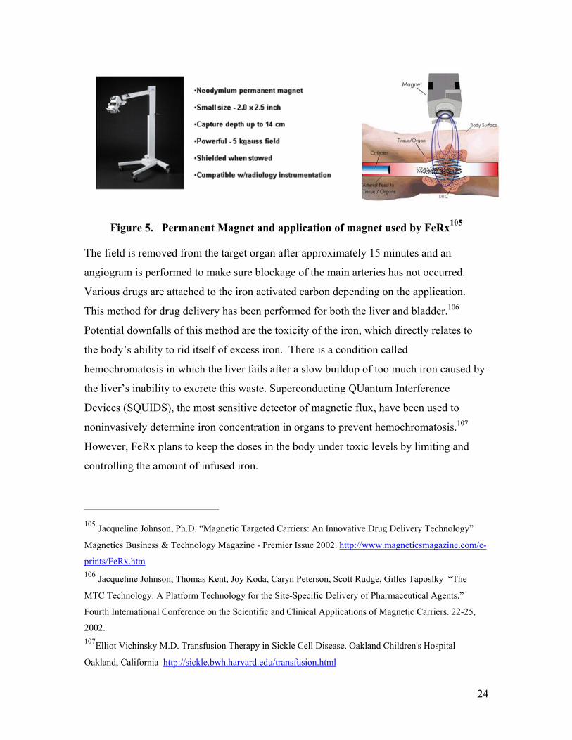
2.3 FeRx Inc.’s Delivery Strategy

In comparison, FeRx has focused on the use of external permanent magnets and particle

transport through tissue. FeRx’s strategy has been to use milled 1 µm iron-activated

carbon which has a much higher magnetic moment when compared to magnetite. Iron is

injected into blood vessels near the target organ and then a single external permanent

magnet pulls the particles out of the bloodstream and into the epithelium layers of the

organ.

104 Stereotaxis, Inc. http://www.stereotaxis.com, 2002.

24

Figure 5. Permanent Magnet and application of magnet used by FeRx105

The field is removed from the target organ after approximately 15 minutes and an

angiogram is performed to make sure blockage of the main arteries has not occurred.

Various drugs are attached to the iron activated carbon depending on the application.

This method for drug delivery has been performed for both the liver and bladder.106

Potential downfalls of this method are the toxicity of the iron, which directly relates to

the body’s ability to rid itself of excess iron. There is a condition called

hemochromatosis in which the liver fails after a slow buildup of too much iron caused by

the liver’s inability to excrete this waste. Superconducting QUantum Interference

Devices (SQUIDS), the most sensitive detector of magnetic flux, have been used to

noninvasively determine iron concentration in organs to prevent hemochromatosis.107

However, FeRx plans to keep the doses in the body under toxic levels by limiting and

controlling the amount of infused iron.

105 Jacqueline Johnson, Ph.D. “Magnetic Targeted Carriers: An Innovative Drug Delivery Technology”

Magnetics Business & Technology Magazine - Premier Issue 2002. http://www.magneticsmagazine.com/e-

prints/FeRx.htm 106 Jacqueline Johnson, Thomas Kent, Joy Koda, Caryn Peterson, Scott Rudge, Gilles Taposlky “The

MTC Technology: A Platform Technology for the Site-Specific Delivery of Pharmaceutical Agents.”

Fourth International Conference on the Scientific and Clinical Applications of Magnetic Carriers. 22-25,

2002. 107Elliot Vichinsky M.D. Transfusion Therapy in Sickle Cell Disease. Oakland Children's Hospital

Oakland, California http://sickle.bwh.harvard.edu/transfusion.html

25

In summary, there have been many uses of magnetic particle manipulation in the human

body. However, a single system has yet to emerge that combines the techniques

presented into a simple tool with a wide range of applications extensively used by the

medical community.

26

Chapter 3: Modeling

This section describes the controlling variables and their interactions in closer detail.

Assumptions about the blood properties, hemodynamic flow conditions, and other

mechanical effects are made here in order to simplify the analysis of in vivo magnetic

guidance.

3.1 Blood Properties

It is important to closely model blood and blood flow in order to engineer an effective

magnetic targeted drug delivery system. Blood consists of plasma, which normally

occupies approximately 55% by volume of the blood, red cells, white cells and platelets.

The red cells are the most numerous and largest, therefore dominating the mechanical

properties of blood. They are flexible disks of approximately 8 µm diameter with a

thickness ranging from 1-3 µm. White cells are similar in size, but are less abundant

compared to the red cells (i.e. 1-2 per 1000 red cells), and they are therefore dynamically

negligible. Platelets number 80-100 per 1000 red cells but are small, round cells with

diameters of 2-4 µm. The platelets’ effects are negligible due to their size and density in

the blood. The plasma consists of a solution of larger molecules, but on the scales of

motion and at the rates of shear normally encountered in the blood vessels, it can be

regarded as a homogeneous Newtonian fluid108 of viscosity109 0.0012-0.0016 kg/(m•s) at

37 °C.

Whole blood cannot be regarded as a Newtonian fluid in blood vessels smaller than 100

µm. Blood also behaves as a shear-thinning fluid whose viscosity varies as a function of 108 A Newtonian fluid is one in which the viscosity coefficient (v) is independent of the

velocity gradient 109 T.J. Pedley, “The fluid mechanics of large blood vessels,” Cambridge University

Press, Cambridge, 1980.

27

shear rate. It is suggested by T.J. Pedley that blood can be considered as a Newtonian

fluid when the shear rate S is greater than 100 s-1 (i.e. the viscosity is independent of the

shear rate). Blood viscosity as a function of shear rate is relatively constant at this limit

as illustrated by Figure 6.

Figure 6. Blood viscosity for men and women with a +/- one standard deviation 110•

This is, however, only true in the regions of the vessel close to the walls. This is in

contrast to the central portion of larger vessels where the velocity profile is nearly

uniform and the shear rate is low. Flow in larger blood vessels is more uniform, termed

“plug” flow, while in smaller blood vessels the flow front shape is more parabolic (Figure

7).

110 Rheologics, Inc. 2001. http://www.rheologics.com/charts.htm

• Note: Viscosity has units of mass/length-time. Poise is the cgs unit of absolute viscosity in g/cm-sec.

To convert from poise to kg/m-sec, divide by 10.

28

Figure 7. Comparison of plug vs parabolic flow of blood in large and small vessels,

respectively.

3.2 Hemodynamic Flow Conditions

Considering the constraints at hand, the calculations that follow are only valid down to

vessels with internal diameters smaller than the carotid artery (approximately 0.6 cm) but

greater than the arteriole system (approximately 10µm-80 µm). If we consider the worst

case (i.e., in the carotid), the mean lumen diameter (internal diameter of the blood vessel)

is 0.6 cm and a measured velocity profile with time is illustrated in Figure 8. Here we see

that the velocity ranges from about 10 to 65 cm/s.

Figure 8. Blood flow in a human carotid artery. 111

111 Jane F. Utting. Measurement of Regional Cerebral Blood Flow

using MRI. University College London. Department of Medical Physics & Bioengineering.

http://www.medphys.ucl.ac.uk/posters99/jfupstr/sld007.htm

29

When the particle size is less then 100 µm and flow velocities are on the order of µm/s or

less, the Reynolds number (Re)112,113 is often less then one. Here,

Re ,Udρµ

= (5)

where ρ is the density of the fluid, U is the free stream velocity, µ is the absolute or

dynamic viscosity, and d is the diameter of the sphere. When the Reynolds number is this

low, forces experienced by the particle are governed primarily by inertial forces. Under

such conditions, the viscous force at low Reynolds numbers is governed by Stokes Law,

F = 6 π η v r, (6)

where η is the viscosity of blood, about 0.004 kg/(m*s), v is the relative velocity of the

fluid, and r is the radius. The flow force is non-stationary (Figure 8), so in general is

more complicated than the simple model shown. However, this model holds at low flow

rates, e.g. in the capillaries.

3.3 Comparison of Hemodynamic Forces with Magnetic Forces

The magnetic force exerted on the microsphere is governed by electromagnetic field and

constitutive relationships. Maxwell’s four equations describe most electromagnetic

phenomenon. They are composed of Faraday’s law, Gauss’s law, a generalization of

Ampère’s law, and a statement of the nonexistence of magnetic monopoles.

Faraday’s law is based on the experimental determination that a time-changing magnetic

flux induces an electromotive force.

S

l xC

d dst tβ βξ ξ∂ ∂

• = − • ∇ = −∂ ∂∫ ∫ (7)

112 E.M. Purcell. “Life at Low Reynolds Number” Lyman Laboratory, Harvard University, Cambridge,

Mass 02138. June 1976. http://brodylab.eng.uci.edu/~jpbrody/reynolds/lowpurcell.html 113 Brody, Austin, Goldstein, & Yager. “Biotechnology at Low Reynolds Numbers”

Biophysical Journal, Dec 1996. http://publish.aps.org/eprint/gateway/eplist/aps1996jul26_001

30

where curve C encloses surface S.

Gauss’s law is based upon Coulomb’s law and experimental determination that electric

charges attract or repel one another with a force inversely proportional to the square of

the distance between them.

dv , DS V

D ds ρ ρ• = ∇• =∫ ∫ (8)

where surface S encloses the volume V.

Ampère’s law states that the line integral of the magnetic field over any closed curve

must equal the total current enclosed by that curve and that the time-varying electric

fields produce magnetic fields.

, x C S S

D DH dl J ds ds H Jt t

∂ ∂• = • + • ∇ = +

∂ ∂∫ ∫ ∫ (9)

where curve C encloses surface S.

Maxwell’s final equation states that no magnetic monopoles exist and that all magnetic

field lines always close on themselves.

0 , 0S

B ds B• = ∇• =∫ (10)

where the surface S encloses a volume V.

The force due to a gradient in a magnetic field is a reduction of the Lorentz force.114 The

Lorentz force )( x )( rBrJdvF ∫= for the case that magnetic flux density B varies

slowly over the extent of the current. We can then expand

( ) (0) ( ) ... ,i i i r oB r B r B == + • ∇ + (11)

114 Discussion with David de Wolf. Electrical and Computer Engineering Department of Virginia Tech.

2002.

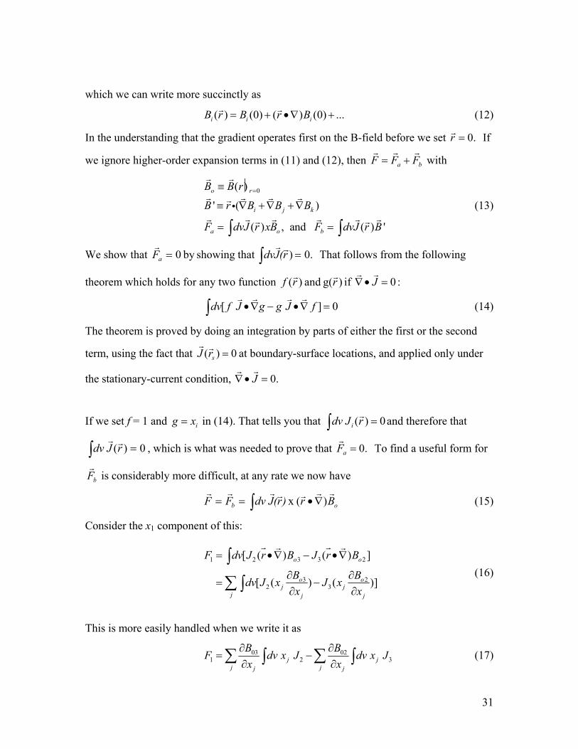
31

which we can write more succinctly as

( ) (0) ( ) (0) ...i i iB r B r B= + •∇ + (12)

In the understanding that the gradient operates first on the B-field before we set .0=r If

we ignore higher-order expansion terms in (11) and (12), then ba FFF += with

0( )

' ( )

( ) , and ( ) '

o r

i j k

a o b

B B r

B r B B B

F dvJ r xB F dvJ r B

=≡

≡ ∇ +∇ +∇

= =∫ ∫i (13)

We show that ∫ == 0. ) that showingby 0 r(JdvFa That follows from the following

theorem which holds for any two function )g( and )( rrf if 0J∇• = :

[ ] 0dv f J g g J f•∇ − •∇ =∫ (14)

The theorem is proved by doing an integration by parts of either the first or the second

term, using the fact that 0)( =srJ at boundary-surface locations, and applied only under

the stationary-current condition, .0=•∇ J

If we set f = 1 and ixg = in (14). That tells you that 0)( =∫ rJdv i and therefore that

0)( =∫ rJdv , which is what was needed to prove that .0=aF To find a useful form for

bF is considerably more difficult, at any rate we now have

ob Br)r(JdvFF )( x ∇•== ∫ (15)

Consider the x1 component of this:

1 2 3 3 2

3 22 3

[ ( ) ( ) ]

[ ( ) ( )]

o o

o oj j

j j j

F dv J r B J r B

B Bdv J x J xx x

= •∇ − •∇

∂ ∂= −

∂ ∂

∫∑∫

(16)

This is more easily handled when we write it as

03 021 2 3 j j

j jj j

B BF dv x J dv x Jx x

∂ ∂= −

∂ ∂∑ ∑∫ ∫ (17)

32

To make this into a form into which we can introduce the magnetic dipole moment

1 ( )2

m dv r J r≡ ×∫ (18)

we make the replacement

1 1 ( ) ( )2 2j k j k k j j k k jdv x J dv x J x J dv x J x J= + + −∫ ∫ ∫ (19)

noting that the first integral is zero, as follows from (14) by setting jf x= and kg x= so

that

1 1 ( ) ( )2 2j k j k k j idv x J dv x J x J dv r J= − = ± ×∫ ∫ ∫ (20)

where i,j,k is either a right-handed (+ sign) or a left handed (- sign) permutation of 1, 2, 3.

Equation (17) now becomes

03 021 2 2 3 3

1 ( ) ( )2 j j j j

j jj j

B BF dv x J x J dv x J x Jx x

∂ ∂= − − −

∂ ∂∑ ∑∫ ∫ (21)

Completing the sum over all possible j we get 4 terms:

03 03 02 021 3 1 2 1

1 3 1 2

1 1( ) ( ) ( ) ( )2 2

B B B BF dv r J dv r J dv r J dv r Jx x x x

∂ ∂ ∂ ∂= × − × + × − ×

∂ ∂ ∂ ∂∫ ∫ ∫ ∫ (22)

or, in terms of components of the magnetic dipole moment:

03 03 02 021 3 1 2 1

1 3 1 2

B B B BF m m m mx x x x

∂ ∂ ∂ ∂= − + −

∂ ∂ ∂ ∂ (23)

which is more succinctly written as

1 2 03 3 02 1( ) ( ) [( ) ]oF m B m B m B= ×∇ − ×∇ = ×∇ × (24)

Doing the same for the other two components of F we find

( ) oF m B= ×∇ × (25)

This can be simplified because m is a constant vector. In simplified derivative notation:

1 3 1 1 3 03 1 2 2 1 02

3 1 03 1 3 03 1 2 02 2 1 02

1 1

( ) ( )( ) ( )

F m m B m m Bm B m B m B m B

m B m B

= ∂ − ∂ − ∂ − ∂= ∂ − ∂ − ∂ − ∂

= •∂ − ∇•

(26)

The last term is zero (Maxwell’s equation). Hence also 3

1

ˆ ( )oi

i i

BF x mx=

∂= •

∂∑ (27)

33

or, using the fact that m is a constant,

( )oF m B= ∇ • (28)

As before, the derivative at r needs to be taken first before setting 0.r =

As a check we consider a current loop in the 0z = plane. The magnetic dipole moment

here is 2 ˆ( ) if m I r z rπ= is the radius of the loop. The Lorentz force is now

F I dl B= ×∫ (29)

so that the gradient force is

( )b oF F I dl r B= = × •∇∫ (30)

with the auxiliary definitions:

ˆ( )

ˆ ˆcos sinˆ ˆ ˆsin cos

dl rd

r x yx y

ϕ ϕ

ϕ ϕϕ ϕ ϕ

=

= += − +

(31)

This transforms into 2

20

0

2

3

1

ˆ ˆ( sin cos ) (cos sin )

ˆ ˆ( )[ ]

ˆ ˆˆ ˆ[ ]

ˆ

y xz z

zi

i i

B BF Ir d x yx y

B BI r x yy x

B BB Bm z y z xy y x xBm x m Bx

π

ϕ ϕ ϕ ϕ ϕ

π

=

∂ ∂= − + × +

∂ ∂

∂ ∂= − × + ×

∂ ∂∂ ∂∂ ∂

= − + − +∂ ∂ ∂ ∂

∂= − ∇•

∂

∫

∑

(32)

Again, the last term is zero (Maxwell’s equation) so that as in (27) and (28) we again find 3 3

1 1

ˆ ˆ ( )ozi i

i ii i

BBF m x x mx x= =

∂∂= = •

∂ ∂∑ ∑ (33)

We will use this result to model the force experienced by magnetic microspheres

synthesized by Dr. Judy Riffle’s research group. In order to calculate the moment of the

magnetic microspheres we will examine the present experimental results obtained by Dr.

Judy Riffle’s research group in the Department of Chemistry at Virginia Tech. They

have successfully synthesized magnetite nanoparticles in 2000 and 5000 g/mol

34

polyethylene oxide. The saturation magnetization of the samples is approximately 20

emu/g (per gram of sample, not per gram of magnetite). It is assumed this can be

increased to at least 30 emu/g and that polylactide can be used as the stabilizer. This

would yield 2 µm polylactide microspheres with a maximum saturation magnetization of

about 30 emu/g. For our field design, if we assume the density of magnetite is 5 g/cm3

and the density of PEO is 1 g/cm3, then at 30 emu/g of material, this is approximately 45

weight percent nanomagnetite. Then if we have 45 g magnetite at a density of 5 g/cm3 it

has a volume of 9 cm3. Thus 55 g PEO at 1 g/cm3 is 55 cm3 of PEO. Therefore, we have

(45 + 55)g/(9 + 55)cm3 which equals an overall particle density of 1.56 g/cm3.

Multiplying the 30 emu/g saturation magnetization by the 1.56g/cm3 density gives 47

emu/cm3 (at saturation) in Gaussian units. Multiplying by 1000 converts the

magnetization to SI units, 47000 A/m. We then calculate the volume for a sphere of 2

µm diameter.

34V=3

rπ (34)

This gives a volume of 3.35 x 10-17 m3 and multiplying this by the moment of the particle

is (47000 A/m)(3.35 x 10-17 m3) = 1.57 x 10-12 A-m2.

For a source magnet having a field of 0.5 T, these particles will be essentially saturated,

i.e. completely aligned, at body temperature. Therefore, in a gradient of 1 Tesla/meter,

the moment is multiplied by the gradient for the magnetic force, which is in the direction

of the field.

A magnetic force of 1.57 x 10-12 A-m2 * 1 T/m = 1.51 x 10-12 N. ¥

¥ 1 Tesla = 1 kg/A-sec2 and 1 Newton = 1 kg-m/sec2

35

It is assumed that the particle should be held stationary in the flow. Using Stokes Law

the maximum drag force is calculated to be 0.00001 m/s and 0.000002 m/s for a viscosity

of 0.004 and 0.02 kg/(m•s), respectively.

The magnetic force is a function of the volume (r3) of the particle and the hemodynamic

drag force is a function the radius (r1). If the magnetic force on the particle is balanced

with the hemodynamic drag force as a function of particle radius at various free stream

velocities U, the crossovers correspond to points of force equilibrium. These conditions

are located at 4.5, 6.4 and 15 µm at velocities of 0.00005, 0.0001, and 0.0005 m/s (Figure

9) for a viscosity of 0.004 kg/(m•s). This calculation provides additional information for

selecting field gradients, particle size, and the required magnetic moments of the

particles.

Viscous and Magnetic Forces Vs. Radii

0.00E+005.00E-111.00E-101.50E-102.00E-102.50E-103.00E-103.50E-104.00E-10

0 2 4 6 8 10

Particle radius (µm)

Forc

e (N

ewto

ns)

Magnetic forceU=0.000005 m/sU=0.00001 m/sU=0.00005 m/sU=0.0001 m/sU=0.0005 m/s

Figure 9. Magnetic and hemodynamic drag forces as a function of particle

radius115

115 Courtesy of Dr. Jack Lesko, ESM Department of Virginia Tech.

36

The capillary flow is approximately 0.00047 m/s116 and their size decreases to ~15 µm.

Therefore an approximately 15 µm diameter magnetite microsphere would be able to

maneuver around most of the capillaries. For the worst case scenario of the full systolic

flow in the artery at 0.7 m/s a 600 µm particle would be needed for stopping the particle

in flow. Comparing different materials gives an additional feel for which parameters

should be most closely controlled. The increase of the moment of the magnetic seed

decreases the needed particle size of the particle to resist the same flow. Therefore, an

increase of moment to 300 emu/g gives a minimum particle size of 5 µm compared to a

15 µm microsphere of magnetite at 0.0005 m/s (flow experienced in the capillaries).

3.4 Other Mechanical Effects

Other mechanical effects also affect guidance. These include tissue porosity and the

allowable cell damage for a given procedure. The amount of magnetic force needed to

pull a particle out of flow can be significantly less then the magnetic force needed to

counteract the drag forces in a stream. FeRx, Inc. is exclusively basing their delivery

strategy on this effect.

116 M. Stücker, V. Baier, T.Reuther, K. Hoffmann, K. Kellam and P. Altmayer, “Capillary Blood Cell

Velocity in Human Skin Capillaries Located Perpendiculary to the Skin Surface: Measured by a new Laser

Doppler Anemometer,” Microvascular Research 52, 188-192 (1996).

(http://www.lawrenz.com/cam1lit2.htm)

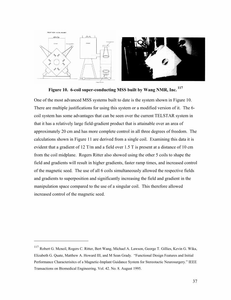
37

Figure 10. 6-coil super-conducting MSS built by Wang NMR, Inc. 117

One of the most advanced MSS systems built to date is the system shown in Figure 10.

There are multiple justifications for using this system or a modified version of it. The 6-

coil system has some advantages that can be seen over the current TELSTAR system in

that it has a relatively large field-gradient product that is attainable over an area of

approximately 20 cm and has more complete control in all three degrees of freedom. The

calculations shown in Figure 11 are derived from a single coil. Examining this data it is

evident that a gradient of 12 T/m and a field over 1.5 T is present at a distance of 10 cm

from the coil midplane. Rogers Ritter also showed using the other 5 coils to shape the

field and gradients will result in higher gradients, faster ramp times, and increased control

of the magnetic seed. The use of all 6 coils simultaneously allowed the respective fields

and gradients to superposition and significantly increasing the field and gradient in the

manipulation space compared to the use of a singular coil. This therefore allowed

increased control of the magnetic seed.

117 Robert G. Mcneil, Rogers C. Ritter, Bert Wang, Michael A. Lawson, George T. Gillies, Kevin G. Wika,

Elizabeth G. Quate, Matthew A. Howard III, and M Sean Grady. “Functional Design Features and Initial

Performance Characterisitcs of a Magnetic-Implant Guidance System for Stereotactic Neurosurgery.” IEEE

Transactions on Biomedical Engineering. Vol. 42. No. 8. August 1995.

38

Figure 11. Calculated field and gradients along the axis for (a) x or y-axis coil, and

(b) z-axis coil for 6-coil superconducting system. The arrows indicate the edge of a

20-cm diameter sphere centered in the region where a head can be located. 117

Using the 6-coil MSS system we will assume we are operating at a 10 T/m gradient and

that the material is in saturation. Only a 200 µm magnetite microsphere is needed to

counteract the full arterial flow at 0.7 m/s and a 4.6 um particle for capillary flow at

0.0005 m/s.

Specifically the assumptions made in this section are the simplification of blood to an

average viscosity, a stationary flow force, and low flow rates such as found in the

capillaries. Other assumptions that are made are the maximum field and gradient that can

be obtained due to cost restraints.

39

Chapter 4: Experimental

This section discusses the design and construction of a magnetic particle guidance

system. The maximum fields and gradients for this system and thus its overall design

were restricted primarily by cost restraints. This system was then modeled using

Ansoft’s 3D Electromagnetic Finite Element Analysis software and compared to

measured values from a Hall probe. The drug delivery vehicle, a magnetic seed, was

characterized using a vibrating sample magnetometer in order to predict a desired

response. Finally, the magnetic seed was investigated under various flow conditions in

vitro to analyze the effectiveness of the drug delivery system.

4.1 Design and Construction of a Magnetic Microsphere Guidance

System

A system was designed for laboratory analysis of magnetic particle guidance. Design

assistance was obtained from Dr. Rogers Ritter and Dr. Duke Creighton at Stereotaxis

Inc. to build a system with a variable field and gradient. Magnet Sales & Manufacturing

Inc. was contracted to construct a variable field and gradient NdFeB permanent magnet

system to the designed specifications.

Integrated Motion was contracted to build in parallel a non-ferric frame, motors, and

controllers to vary the field and gradient over a set area. The motors were designed to

withstand non-linear forces experienced by the magnets with a calculated maximum pull

of 500 lbs per magnet. A minimum separation of 0.5 inches was ensured between the

field magnets. The system had a variable field and gradient from 0-0.5T and 0-13 T/m

respectively over a range of volumes.

Design and construction of an improved magnetic microsphere investigation system was

completed (Figure 12). The frame was made of extruded aluminum and bolted to a lab

bench for structural stability. The actuators used were WM60 Precision Technology

40

Figure 12. Variable magnetic field and gradient test system.

ServosController

Field Magnets

Gradient Magnet

Motors

Actuators

X

Z

Y

Z

Y

X

41

Figure 13. Wiesel Powerline WM60 Actuator. The actuator consists of a sliding

carriage(1), scraper brushes(2), tubular section with sliding bars(3), ball screw(4),

guideway for screw supports(5), guideways(6), covering strip(7), ball-bearing guided

carriage(8), ball nut unit(10), bearing housing and fixed bearing(11).118

Wiesel Powerline that had a 100 mm travel with a 650 mm total length (Figure 13). The

motors used were Goldline XT with 1.81 lb-ft continuous torque at stall, 4.35 lb-ft peak

torque at stall, maximum speed of 6000 rpm, brushless servo motors with single speed

resolver (Figure 14). The servos used were a Servostar brushless servo amplifier with

integrated power supply rated at 3 amps continuous power (Figure 15).

The original system’s magnets that Stereotaxis used were relatively free moving

compared with the improved system. This allowed a maximum field of 0.1T and a

gradient of 1 T/m. In the original system developed at Stereotaxis if the end field

magnets were moved closer together in order to increase the field and gradient, also

118 Wiesel Powerline Product Literature. NEFF Antriebstechnik Automation GmbH. April 1, 2002.

42

decreasing the available workspace, the magnets would overcome the small frictional

forces that were present and become lodged together. A higher field and gradient with

the addition of motors and actuators allowed the magnets to be moved closer together and

resist the attractive forces of the magnet. The variable magnetic field and gradient test

system allows us to achieve high fields and gradients with a large workspace. The large

magnetic workspace also allows us to in the future visually monitor the microspheres

using a microscope equipped with long working distance objectives.

Figure 14. Diagram of Goldline XT MT(B)304 Motor.119

119 Kollmorgen GOLDLINETM XT Brushless Series Motors -30 Frame Size. Product Literature. 2002.

43

Figure 15. Servostar brushless servo amplifier with integrated power supply.

A laptop was used as a controller interfaced by a RS-232 port to the system’s actuators.

Kollmorgen’s Servostar software running on the laptop was used to program the

actuators. The field magnets position, velocity, and the timing of their movement can be

controlled directly through the software (Figure 16).

Figure 16. Kollmorgen’s Servostar Motionlink software.

44

Figure 17. Various grades of NdFeB. 120

The grade of NdFeB used to construct the magnets was 48M. This grade is one of the highest performance NdFeB available (Figure 17). N48M has the following characteristics: Relative permeability (Mu) 1.45

Conductivity 6.2 S/m

Coercitivity (Hc) 14000 kA/m

Remanence (Br) 1.36-1.41 T

Maximum Energy Product (BH)max 358-390-kJ/m^3

Table 9. Properties of N48M.

These characteristics were used later in the electromagnetic finite element analysis.

120Shin-Etsu Magnetics Inc.

http://www.shinetsumagnetics.com/n_series_magnetic_performance_di.htm

45

4.2 Characterization of Field and Gradient

A THM 7025 3-Axis Hall Teslameter was used to accurately measure and spatially map

the field and gradient of the system. Three Hall elements are used in this device to

measure the different components of the B field. The elements that measure Bx, By and

Bz are located within a 3mm diameter sphere at the end of the probe. One can assume

that the center of this sphere is approximately the center of the active sensor volume with

a range of 0.01 mT- 2 T (Figure 18).

Figure 18. The THM 7025 3-Axis Hall Teslameter121

121 MetroLab THM 7025 Users Manual. Version 2.01. Revision 1.4. September 1997.

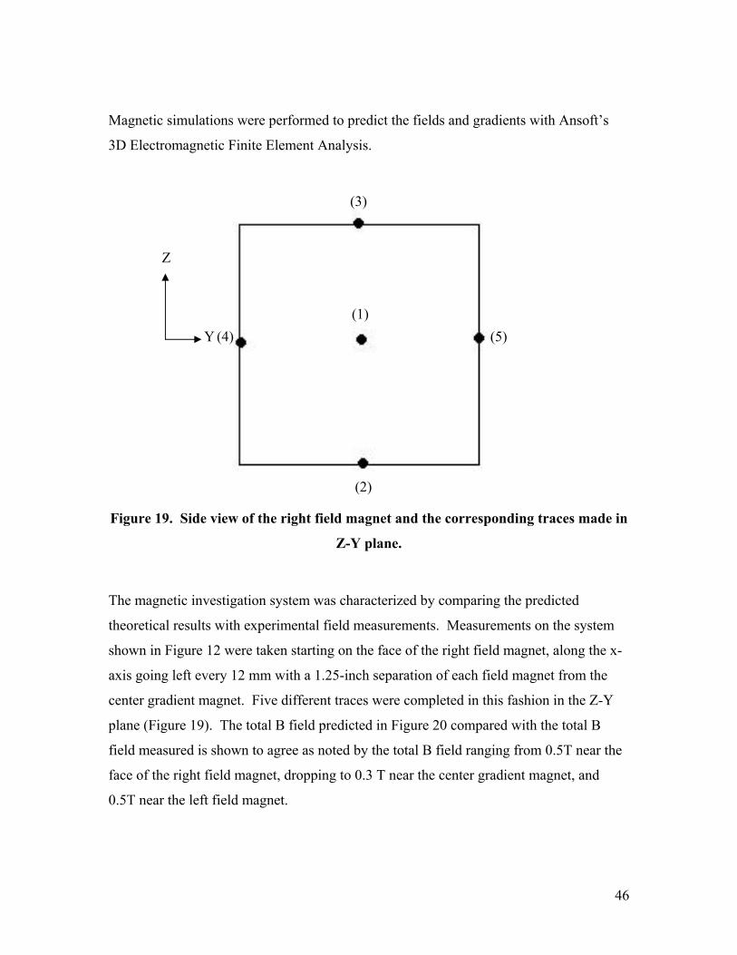
46

Magnetic simulations were performed to predict the fields and gradients with Ansoft’s

3D Electromagnetic Finite Element Analysis.

Figure 19. Side view of the right field magnet and the corresponding traces made in

Z-Y plane.

The magnetic investigation system was characterized by comparing the predicted

theoretical results with experimental field measurements. Measurements on the system

shown in Figure 12 were taken starting on the face of the right field magnet, along the x-

axis going left every 12 mm with a 1.25-inch separation of each field magnet from the

center gradient magnet. Five different traces were completed in this fashion in the Z-Y

plane (Figure 19). The total B field predicted in Figure 20 compared with the total B

field measured is shown to agree as noted by the total B field ranging from 0.5T near the

face of the right field magnet, dropping to 0.3 T near the center gradient magnet, and

0.5T near the left field magnet.

Z

Y (1)

(2)

(3)

(4) (5)

47

TOTAL MEASURED B FIELD

CENTERLINE (1) BOTTOM (2) TOP (3) FAR (4) NEAR (5)

0.548 0.48 0.571 0.514 0.546

0.464 0.356 0.418 0.371 0.523

0.368 0.298 0.267 0.263 0.284

0.314 0.272 0.186 0.196 0.118

0.387 0.315 0.342 0.378 0.324

0.44 0.372 0.45 0.444 0.4

0.587 0.565 0.669 0.635 0.534

Figure 20. Theoretical field strengths predicted using ANSOFT’s 3D Maxwell

Equation Finite Element Analysis Software compared to measured values.

48

TOTAL X -COMPONENT OF B FIELD

CENTERLINE (1) BOTTOM (2) TOP (3) FAR (4) NEAR (5)

-0.55 -0.252 -0.478 -0.417 -0.421

-0.481 -0.268 -0.365 -0.324 -0.252

-0.376 -0.227 -0.264 -0.312 -0.27

-0.292 -0.1609 -0.197 -0.1609 -0.1094

-0.407 -0.271 -0.24 -0.312 -0.261

-0.462 -0.262 -0.257 -0.36 -0.277

-0.594 -0.496 -0.508 -0.433 -0.445

Figure 21. Total X-Component of B Field.

The total x-component of the B field predicted in Figure 21 compared with the total x-

component of the B field measured is shown to agree as noted by the B field ranging

from 0.5T near the face of the right field magnet, dropping to 0.3 T near the center

gradient magnet, and 0.5T near the left field magnet.

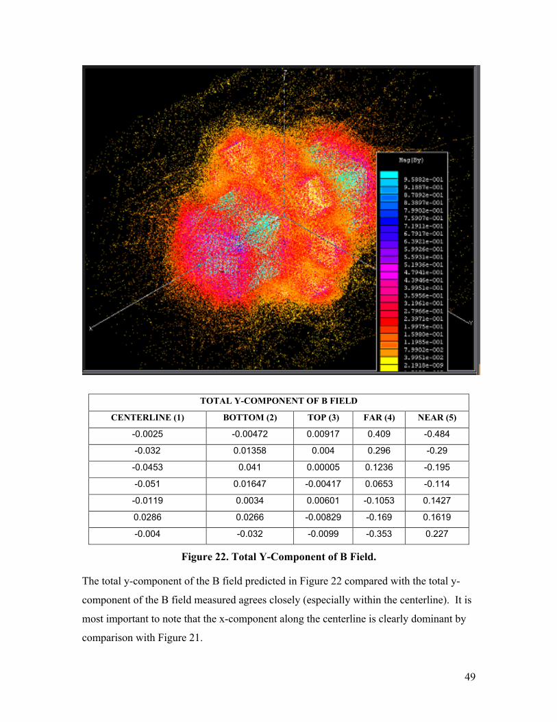
49

TOTAL Y-COMPONENT OF B FIELD

CENTERLINE (1) BOTTOM (2) TOP (3) FAR (4) NEAR (5)

-0.0025 -0.00472 0.00917 0.409 -0.484

-0.032 0.01358 0.004 0.296 -0.29

-0.0453 0.041 0.00005 0.1236 -0.195

-0.051 0.01647 -0.00417 0.0653 -0.114

-0.0119 0.0034 0.00601 -0.1053 0.1427

0.0286 0.0266 -0.00829 -0.169 0.1619

-0.004 -0.032 -0.0099 -0.353 0.227

Figure 22. Total Y-Component of B Field.

The total y-component of the B field predicted in Figure 22 compared with the total y-

component of the B field measured agrees closely (especially within the centerline). It is

most important to note that the x-component along the centerline is clearly dominant by

comparison with Figure 21.

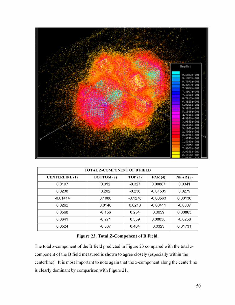
50

TOTAL Z-COMPONENT OF B FIELD

CENTERLINE (1) BOTTOM (2) TOP (3) FAR (4) NEAR (5)

0.0197 0.312 -0.327 0.00887 0.0341

0.0238 0.202 -0.236 -0.01535 0.0279

-0.01414 0.1086 -0.1276 -0.00563 0.00136

0.0262 0.0146 0.0213 -0.00411 -0.0007

0.0568 -0.156 0.254 0.0059 0.00863

0.0641 -0.271 0.339 0.00038 -0.0258

0.0524 -0.367 0.404 0.0323 0.01731

Figure 23. Total Z-Component of B Field.

The total z-component of the B field predicted in Figure 23 compared with the total z-

component of the B field measured is shown to agree closely (especially within the

centerline). It is most important to note again that the x-component along the centerline

is clearly dominant by comparison with Figure 21.

51

TOTAL X-COMPONENT GRADIENT OF B FIELD

CENTERLINE (1) BOTTOM (2) TOP (3) FAR (4) NEAR (5)

-5.7500 1.3333 -9.4167 -7.7500 -14.0833

-8.7500 -3.4167 -8.4167 -1.0000 1.5000

-7.0000 -5.5083 -5.5833 -12.5917 -13.3833

9.5833 9.1750 3.5833 12.5917 12.6333

4.5833 -0.7500 1.4167 4.0000 1.3333

11.0000 19.5000 20.9167 6.0833 14.0000

Figure 24. Total X-Component Gradient of B Field.

The total x-component gradient of the B field predicted in Figure 24 compared with the

total x-component of the B field measured is shown to agree closely (especially along the

centerline).

52

TOTAL Y-COMPONENT GRADIENT OF B FIELD

CENTERLINE (1) BOTTOM (2) TOP (3) FAR (4) NEAR (5)

2.4583 -1.5250 0.4308 9.4167 -16.1667

1.1083 -2.2850 0.3292 14.3667 -7.9167

0.4750 2.0442 0.3517 4.8583 -6.7500

-3.2583 1.0892 -0.8483 14.2167 -21.3917

-3.3750 -1.9333 1.1917 5.3083 -1.6000

2.7167 4.8833 0.1342 15.3333 -5.4250

Figure 25. Total Y-Component Gradient of B Field.

The total y-component gradient of the B field predicted in Figure 25 compared with the

total z-component of the B field measured agree closely (especially within the

centerline). It is most important to note again that the y-component along the centerline

is dominant by comparison with Figure 24 and the higher variance shown in the values of

Figure 25.

53

TOTAL Z-COMPONENT GRADIENT OF B FIELD

CENTERLINE (1) BOTTOM (2) TOP (3) FAR (4) NEAR (5)

-0.3417 9.1667 -7.5833 2.0183 0.5167

3.1617 7.7833 -9.0333 -0.8100 2.2117

-3.3617 7.8333 -12.4083 -0.1267 0.1717

-2.5500 14.2167 -19.3917 -0.8342 -0.7775

-0.6083 9.5833 -7.0833 0.4600 2.8692

0.9750 8.0000 -5.4167 -2.6600 -3.5925

Figure 26. Total Z-Component Gradient of B Field.

The total z-component gradient of the B field predicted in Figure 26 compared with the

total z-component of the B field measured tend to agree (especially within the centerline).

It is most important to note again that the z-component along the centerline is dominant

by comparison with Figure 24 and the higher variance shown in the values of Figure 25.

54

TOTAL X-COMPONENT GRADIENT OF B FIELD * X-COMPONENT OF B FIELD

CENTERLINE (1) BOTTOM (2) TOP (3) FAR (4) NEAR (5)

3.1625 -0.3360 4.5012 3.2318 5.9291

4.2088 0.9157 3.0721 0.3240 -0.3780

2.6320 1.2504 1.4740 3.9286 3.6135

-2.7983 -1.4763 -0.7059 -2.0260 -1.3821

-1.8654 0.2033 -0.3400 -1.2480 -0.3480

-5.0820 -5.1090 -5.3756 -2.1900 -3.8780

Figure 27. Total X-Component Gradient of B Field * X-Component of B Field.

The total product of the x-component gradient and the x-component of the B field

predicted in Figure 27 compared with the product of the x-component gradient and the x-

component of the B field measured is shown to agree as noted by values ranging close to

one within the predicted and experimental values.

55

TOTAL Y-COMPONENT GRADIENT OF B FIELD * Y-COMPONENT OF B FIELD

CENTERLINE (1) BOTTOM (2) TOP (3) FAR (4) NEAR (5)

-0.0061 0.0072 0.0040 3.8514 7.8247

-0.0355 -0.0310 0.0013 4.2525 2.2958

-0.0215 0.0838 0.0000 0.6005 1.3163

0.1662 0.0179 0.0035 0.9283 2.4387

0.0402 -0.0066 0.0072 -0.5590 -0.2283

0.0777 0.1299 -0.0011 -2.5913 -0.8783

Figure 28. Total Y-Component Gradient of B Field * Y-Component of B Field.

The total product of the y-component gradient and the y-component of the B field

predicted in Figure 28 compared with the product of the y-component gradient and the y-

component measured it is important to note the lower magnitude and higher variance to

that of the total product of the x-component gradient and the x-component of the B field.

56

TOTAL Z-COMPONENT GRADIENT OF B FIELD * Z-COMPONENT OF B FIELD

CENTERLINE (1) BOTTOM (2) TOP (3) FAR (4) NEAR (5)

-0.0067 2.8600 2.4798 0.0179 0.0176

0.0752 1.5722 2.1319 0.0124 0.0617

0.0475 0.8507 1.5833 0.0007 0.0002

-0.0668 0.2076 -0.4130 0.0034 0.0005

-0.0346 -1.4950 -1.7992 0.0027 0.0248

0.0625 -2.1680 -1.8363 -0.0010 0.0927

Figure 29. Total Z-Component Gradient of B Field * Z-Component of B Field.

The total product of the z-component gradient and the z-component of the B field

predicted in Figure 29 compared with the product of the z-component gradient and the z-

component measured it is important to note the lower magnitude and higher variance to

that of the total product of the x-component gradient and the x-component of the B field.

57

Figure 30. Composite View. From left to right: (a)Magnitude of Field in the x-

plane, y-plane, and z-plane. (b) Gradient in the x-plane, y-plane, and z-plane. (c)

Field-Gradient product in the x-plane, y-plane and z-plane.

The constituent analysis of the field and gradient in every direction and volume was

performed to characterize the workspace between the magnets. Since the field and

gradient varied over the entire workspace volume, we needed to find the volume elements

with the highest field and gradient with the smallest amount of variation in a given

volume. The chosen experimental volume of 0.64 cm3 meeting these criteria is located

on the right face of the center gradient magnet (offset from the geometric center of the

circular gradient magnet).

4.3 Characterization of Magnetic Microspheres

Magnetic properties of microspheres containing magnetite nanoparticles were

characterized via vibrating sample magnetometry (Figure 31). The vibrating sample

magnetometer operates on the principle that when a sample material is placed in a

(a)

(b)

(c)

58

uniform magnetic field, a dipole moment proportional to the product of the sample

susceptibility times the applied field is induced in the sample. A sample also undergoing

sinusoidal motion induces an electrical signal in a set of stationary pick-up coils. This

signal is proportional to the magnetic moment, vibration amplitude, and vibration

frequency.

Figure 31. The LakeShore 7300 Vibrating Sample Magnetometer.

The material under study is contained in a sample holder, which is centered in the region

between the pole pieces of an electromagnet. A vertical sample rod connects the sample

holder with a transducer assembly located above the magnet, which supports the

transducer assembly with sturdy, adjustable support rods. The transducer then converts a

sinusoidal AC drive signal, provided by a circuit located in the console, into a sinusoidal

vertical vibration of the sample rod, and the sample thus undergoes a sinusoidal motion in

a uniform magnetic field. Coils mounted on the pole pieces of the magnet pick up the

signal resulting from the sample motion. This AC signal at the vibration frequency is

proportional to the magnitude of the moment induced in the sample, vibration amplitude

and frequency. A servo system maintains constancy in the drive amplitude and frequency

so that the output accurately tracks the moment level without degradation due to

variations in the amplitude and frequency of vibration. The complete system operation is

summarized in Figure 32.

59

Figure 32. Flowchart of VSM operations.122

The samples can be characterized by weight or volume. Dry microsphere samples were

weighed and fluids were injected into the sample holder (0.05 mL). The VSM was

ramped to full field and the highest sensitivity allowed for the selected material. The

field was ramped from 0.8 T to –0.8T and back to 0.8 T over a period of 30 minutes. An

exemplary magnetic response for Dynabeads Product 142.04 (Table 10), is provided in

Figure 33. This material was in the form of uniform, superparamagnetic, polystyrene

beads coated with a polyurethane layer. The data confirmed that these microspheres did

not exhibit hysteresis as in (Figure 34).

122 User’s Manual. Lakeshore 7300 Series. VSM System. February 2001.

60

Physical characteristics

Diameter 2.8 µm ± 0.2 µm (C.V. max 5%)

Surface area 4-8 m2/g

Active chemical functionality 50-70 µmol/g Dynabeads

Density 1.3 g/cm3

Iron content approx. 12%

Magnetic mass susceptibility 100 ± 25 x 10-6 m3/kg

Concentration 2 x 109 beads/ml (approx. 30 mg/ml)

Table 10. Physical Characteristics of Dynabeads M-280 Magnetic Microspheres.123

Magnetic Response of Dynabeads-Prod 142.04

-0.30

-0.20

-0.10

0.00

0.10

0.20

0.30

-8000 -6000 -4000 -2000 0 2000 4000 6000 8000

Field (Gauss)

Mom

ent (

emu/

g)

Figure 33. VSM Characterization of Dynabeads Product Number 142.04.

123 Product Literature for Dynal Biotech Product Number 142.04. 2001.

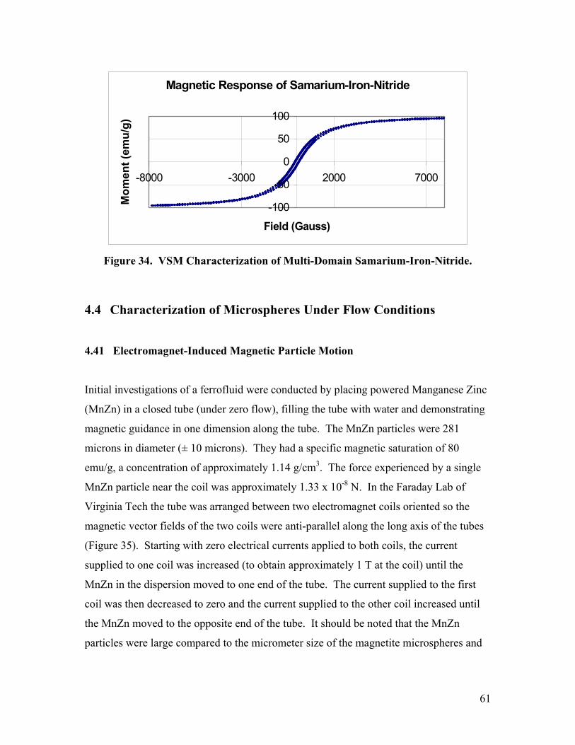
61

Figure 34. VSM Characterization of Multi-Domain Samarium-Iron-Nitride.

4.4 Characterization of Microspheres Under Flow Conditions

4.41 Electromagnet-Induced Magnetic Particle Motion

Initial investigations of a ferrofluid were conducted by placing powered Manganese Zinc

(MnZn) in a closed tube (under zero flow), filling the tube with water and demonstrating

magnetic guidance in one dimension along the tube. The MnZn particles were 281

microns in diameter (± 10 microns). They had a specific magnetic saturation of 80

emu/g, a concentration of approximately 1.14 g/cm3. The force experienced by a single

MnZn particle near the coil was approximately 1.33 x 10-8 N. In the Faraday Lab of

Virginia Tech the tube was arranged between two electromagnet coils oriented so the

magnetic vector fields of the two coils were anti-parallel along the long axis of the tubes

(Figure 35). Starting with zero electrical currents applied to both coils, the current

supplied to one coil was increased (to obtain approximately 1 T at the coil) until the

MnZn in the dispersion moved to one end of the tube. The current supplied to the first

coil was then decreased to zero and the current supplied to the other coil increased until

the MnZn moved to the opposite end of the tube. It should be noted that the MnZn

particles were large compared to the micrometer size of the magnetite microspheres and

Magnetic Response of Samarium-Iron-Nitride

-100

-50

0

50

100

-8000 -3000 2000 7000

Field (Gauss)

Mom

ent (

emu/

g)

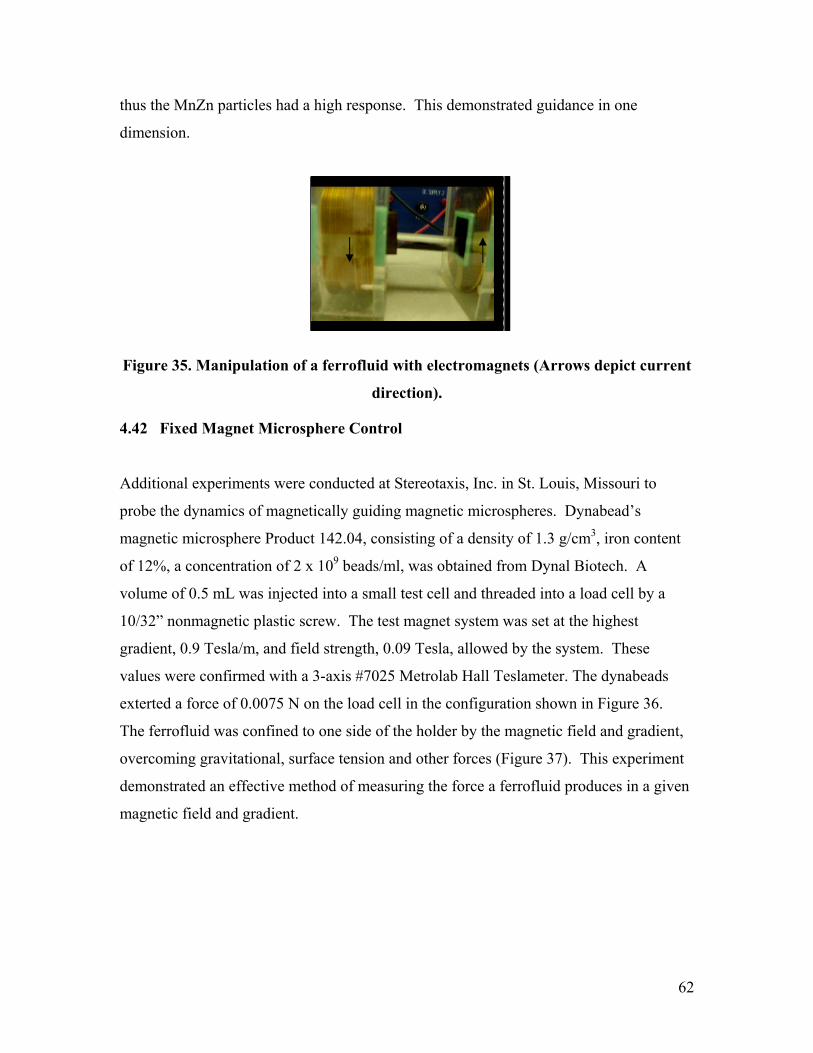
62

thus the MnZn particles had a high response. This demonstrated guidance in one

dimension.

Figure 35. Manipulation of a ferrofluid with electromagnets (Arrows depict current

direction).

4.42 Fixed Magnet Microsphere Control

Additional experiments were conducted at Stereotaxis, Inc. in St. Louis, Missouri to

probe the dynamics of magnetically guiding magnetic microspheres. Dynabead’s

magnetic microsphere Product 142.04, consisting of a density of 1.3 g/cm3, iron content

of 12%, a concentration of 2 x 109 beads/ml, was obtained from Dynal Biotech. A

volume of 0.5 mL was injected into a small test cell and threaded into a load cell by a

10/32” nonmagnetic plastic screw. The test magnet system was set at the highest

gradient, 0.9 Tesla/m, and field strength, 0.09 Tesla, allowed by the system. These

values were confirmed with a 3-axis #7025 Metrolab Hall Teslameter. The dynabeads

exterted a force of 0.0075 N on the load cell in the configuration shown in Figure 36.

The ferrofluid was confined to one side of the holder by the magnetic field and gradient,

overcoming gravitational, surface tension and other forces (Figure 37). This experiment

demonstrated an effective method of measuring the force a ferrofluid produces in a given

magnetic field and gradient.

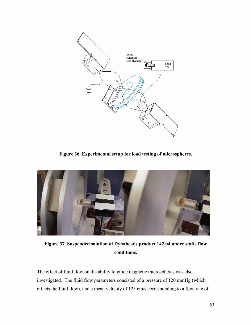
63

Figure 36. Experimental setup for load testing of microspheres.

Figure 37. Suspended solution of Dynabeads product 142.04 under static flow

conditions.

The effect of fluid flow on the ability to guide magnetic microspheres was also

investigated. The fluid flow parameters consisted of a pressure of 120 mmHg (which

effects the fluid flow), and a mean velocity of 125 cm/s corresponding to a flow rate of

64

1.9 liters/minute. A fluid consisting of 5% glycerol and 95% water was used to simulate

the viscosity of blood. The fluid flowed through a 0.4 cm (~3/16”) inner diameter tube

pumped by a Cole-Parmer SY-07554-90 Masterflex L/S Economy Drive Pump with SY-

2201-62 Easy-Load Pump Head. This was considered a challenging set of conditions

where guidance and control of the magnetic particles was needed.

The 5% glycerol (26 mL), 95% water (500mL), and 0.4mL of the dynabead solution was

mixed in a Nalgene bottle to give a brownish dispersion. All fields and gradients were

kept identical to the previous experiment while 3/16” inner diameter Nalgene tubing was

fed through the center of the magnet (Figure 38). The pump flow was varied from zero

flow to the full flow, 125 cm/s. It was observed that the dynabeads remained dispersed in

the solution and did not congregate in the magnetic field. This was due to an insufficient

magnetic force to counteract the drag force due to a high stream velocity.

Figure 38. Suspended solution of Dynabeads product 142.04 under dynamic flow

conditions.

The dynabeads were also injected directly into the tubing within the magnetic field at

zero flow (Figure 39). This approach kept the dynabeads from dispersing in the solution.

The field and gradient were sufficient to hold the particles in place with relatively no

flow. However, there was not sufficient strength to hold the ferro-fluid in place at 1/10

the fluid flow, 12.5 cm/s, that would be experienced in the main arteries. This however

does suggest that guidance is possible in a static or low velocity system where the blood

flow is temporarily reduced.

65

Figure 39. Suspended solution of Dynabead’s product 142.04 under variable

static/dynamic flow conditions.

4.43 Magnetic Guidance Using Permanent Magnet System at Virginia Tech

Additional experiments with smaller tubing, lower velocities and flow rates, and a higher

field-gradient in the new magnetic investigation system were conducted with the

objective of confining a group of magnetic microspheres to one side of the tubing during

fluid flow (Figure 40). Silicone tubing (Cole Parmer with a 0.64 mm inner diameter) was

filled with water using a BD disposable syringe equipped with a Leur-Lok 23 gauge

needle.

Magnetic

microspheres

66

Figure 40. Suspended solution of Dynabead’s product 142.04 under dynamic flow

conditions with higher field-gradient, smaller tubing size, and slower flow

conditions.

Five mL of Dynabead’s magnetic microsphere Product 142.04 was injected into the water

filled tubing at a rate of approximately 1 ml/min (0.05 cm/s). The tubing was placed in

an axial field of 0.3T and a gradient of 13 T/m. The field and gradient component in the

other two lines of space was significantly lower compared to the axial direction.

Agglomeration of the microspheres or a shift to one side of the tube was not witnessed in

this experiment and it appeared that the governing force on microsphere guidance was the

fluid flow at 1 ml/min. The magnetic force was expected to be insufficient to hold the

Dynabeads stationary in the center of the fluid flow, however it was theorized that

frictional forces pushing the Dynabeads against the side of the tubing may allow for

agglomeration. Agglomeration of the microspheres may be witnessed with better

visualization tools.

Calculations discussed in Section 3.3 indicated that using a 0.3T field and a gradient of

13 T/m, there would be enough magnetic force to manipulate a particle with larger mass

at a flow rate of 1 mL/min. An Olympus AX-70 Confocal microscope was used to

measure the particle size of a sample of MnZn. Examination of 5 MnZn particles

displayed a uniform size of 281 ± 10 microns (Figure 41) and was found to have a

magnetic moment of 80 emu/g (Figure 42).

Direction of

Magnetic

Force

67

Figure 41. Characteristic 281 micron MnZn sample.

Magnetic Response of MnZn Sample

-100

-50

0

50

100

-10000 -5000 0 5000 10000

Field (Gauss)

Mag

netic

Mom

ent

(em

u/g)

Figure 42. VSM Characterization of MnZn.

This hypothesis held true when tested (Figure 43). 1 cc MnZn powder was mixed with 20

cc of deionized water, and injected through tubing at a rate of 1 mL/min. It was observed

that the MnZn was suspended against the side of the tubing while deionized water flowed

past.

68

MnZn particles suspended during flow

Figure 43. Suspended solution of MnZn under dynamic flow conditions with higher

field-gradient, smaller tubing size, and slower flow conditions.

Additional experiments with dynamic field and gradient conditions with flow needed to

be conducted to further demonstrate magnetic guidance. In this series of experiments the

magnets were moved both away and in parallel to the tubing to vary the magnetic force.

Silicone tubing (Cole Parmer with a 0.64 mm inner diameter) was filled with water using

a BD disposable syringe equipped with a Leur-Lok 23 gauge needle. 1 cc MnZn powder

was mixed with 20 cc of deionized water, and injected through tubing at a rate of 1

mL/min. The tubing was placed in an axial field of 0.3T and a gradient of 13 T/m,

parallel to the lab bench. It was again observed that the MnZn was suspended against the

side of the tubing while deionized water flowed (Figure 44.a) past since the field and

gradient component in the other two lines of space were a couple of degrees of magnitude

lower compared to the axial direction as discussed in section 4.2.

Direction of

Magnetic

Force

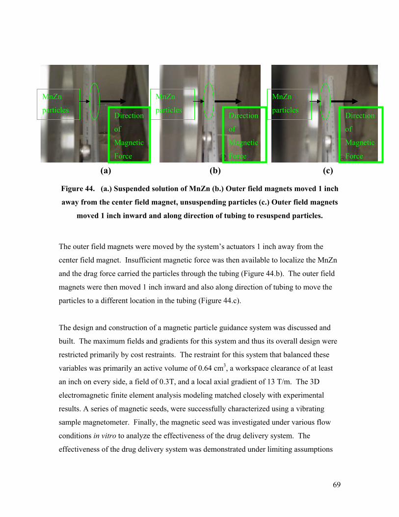
69

Figure 44. (a.) Suspended solution of MnZn (b.) Outer field magnets moved 1 inch

away from the center field magnet, unsuspending particles (c.) Outer field magnets

moved 1 inch inward and along direction of tubing to resuspend particles.

The outer field magnets were moved by the system’s actuators 1 inch away from the

center field magnet. Insufficient magnetic force was then available to localize the MnZn

and the drag force carried the particles through the tubing (Figure 44.b). The outer field

magnets were then moved 1 inch inward and also along direction of tubing to move the

particles to a different location in the tubing (Figure 44.c).

The design and construction of a magnetic particle guidance system was discussed and

built. The maximum fields and gradients for this system and thus its overall design were

restricted primarily by cost restraints. The restraint for this system that balanced these

variables was primarily an active volume of 0.64 cm3, a workspace clearance of at least

an inch on every side, a field of 0.3T, and a local axial gradient of 13 T/m. The 3D

electromagnetic finite element analysis modeling matched closely with experimental

results. A series of magnetic seeds, were successfully characterized using a vibrating

sample magnetometer. Finally, the magnetic seed was investigated under various flow

conditions in vitro to analyze the effectiveness of the drug delivery system. The

effectiveness of the drug delivery system was demonstrated under limiting assumptions

(a) (b) (c)

MnZn

particles Direction

of

Magnetic

Force

MnZn

particles Direction

of

Magnetic

Force

MnZn

particles Direction

of

Magnetic

Force

70

of a specific magnetic field and gradient, seed material, a low fluid flow, and a small

volume.

71

Chapter 5: Conclusion

This thesis reviewed past magnetic drug delivery work, variables, and concepts that

needed to be understood for the development of an in vivo magnetic drug delivery

system. The results of this thesis are the concise study and review of present methods for

guided magnetic particles, aggregate theoretical work to allow proper hypotheses and

extrapolations to be made, and experimental applications of these hypotheses to a

working magnetic guidance system. There have been many uses of magnetic particle

manipulation in the human body. However, a single system has yet to emerge that

combines those techniques into a simple tool with a wide range of applications

extensively used by the medical community.

Specifically the assumptions made in this thesis are the simplification of blood to an

average viscosity, a stationary flow force, and low flow rates such as found in the

capillaries. Other assumptions that are made are the maximum field and gradient that can

be obtained due to cost restraints.

The design and construction of a magnetic particle guidance system was discussed and

built. The restraint for this system that balanced multiple competing variables was

primarily an active volume of 0.64 cm3, a workspace clearance of at least an inch on

every side, a field of 0.3T, and a local axial gradient of 13 T/m. The 3D electromagnetic

finite element analysis modeling performed matched closely with experimental results. A

series of magnetic seeds, were successfully characterized using a vibrating sample

magnetometer. Finally, the magnetic seed was investigated under various flow

conditions in vitro to analyze the effectiveness of the drug delivery system. The

effectiveness of the drug delivery system was demonstrated under limiting assumptions

of a specific magnetic field and gradient, seed material, a low fluid flow, and a small

volume. The conclusions of this thesis are that magnetic targeted drug delivery is a

viable technology and is still in its infancy and there is still much work to be completed

before a clinical solution will fully emerge.

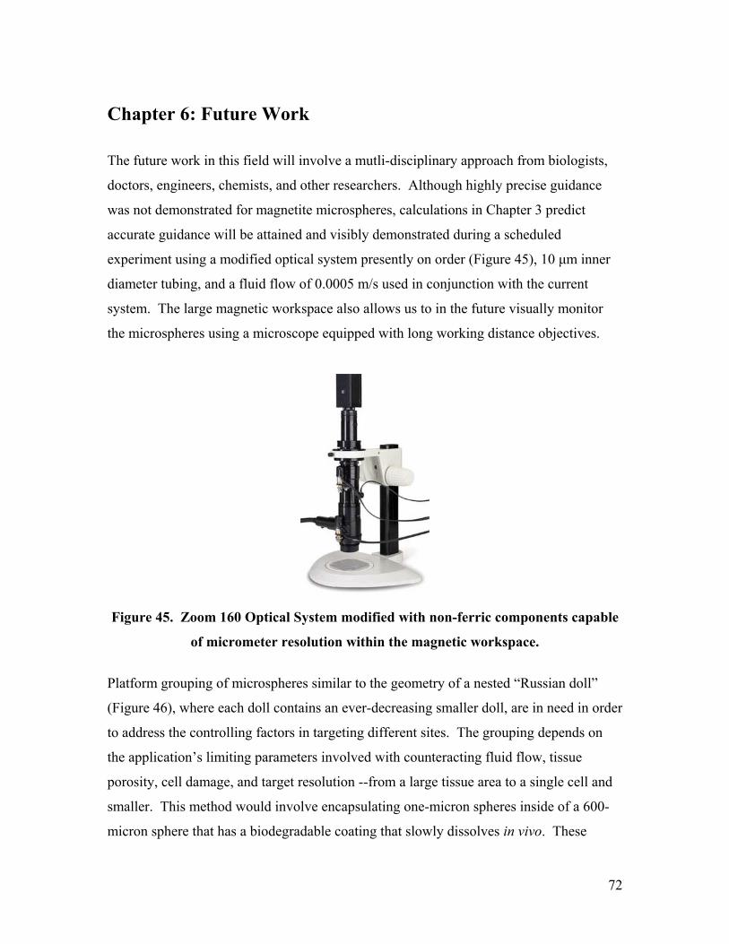
72

Chapter 6: Future Work

The future work in this field will involve a mutli-disciplinary approach from biologists,

doctors, engineers, chemists, and other researchers. Although highly precise guidance

was not demonstrated for magnetite microspheres, calculations in Chapter 3 predict

accurate guidance will be attained and visibly demonstrated during a scheduled

experiment using a modified optical system presently on order (Figure 45), 10 µm inner

diameter tubing, and a fluid flow of 0.0005 m/s used in conjunction with the current

system. The large magnetic workspace also allows us to in the future visually monitor

the microspheres using a microscope equipped with long working distance objectives.

Figure 45. Zoom 160 Optical System modified with non-ferric components capable

of micrometer resolution within the magnetic workspace.

Platform grouping of microspheres similar to the geometry of a nested “Russian doll”

(Figure 46), where each doll contains an ever-decreasing smaller doll, are in need in order

to address the controlling factors in targeting different sites. The grouping depends on

the application’s limiting parameters involved with counteracting fluid flow, tissue

porosity, cell damage, and target resolution --from a large tissue area to a single cell and

smaller. This method would involve encapsulating one-micron spheres inside of a 600-

micron sphere that has a biodegradable coating that slowly dissolves in vivo. These

73

coatings generally take from hours to days to dissolve and release the smaller inner

spheres. It has also been suggested that using multiple hydrogen bonding will give a

similar fast unraveling capability that DNA does at 105°F. RF induction heating is one

method that could give localized heating to break up the larger volume of magnetic

microspheres into smaller more maneuverable spheres. This heating will take place when

the carriers attempt to maneuver into smaller passageways and need the advantages that a

smaller transport offers. These factors on the chemistry side of the magnetic drug

delivery system need to be realized in order to maximize the targeting resolution of the

magnetic stereotactic system.

Figure 46. Platform grouping of microspheres.

A more compact and efficient design then the 5th generation MSS, 6-coil superconducting

system could be implemented using MRI technology. The RF coils would take much less

room then the fluoroscope hardware and would allow for larger fields/gradients since not

all of the coils would have to be open bore to allow for imaging. The current procedure

that Stereotaxis uses is to place the patient in a commercial MRI to get a roadmap of the

pathway of interest and to update the position of the magnetic seed on that roadmap with

data derived from the fluoroscope. The incorporation of MRI into the stereotaxis device

will shorten and simplify the procedure that Stereotaxis, Inc. has followed in its current

use of the TELSTAR to guide magnet tip catheters through the brain. The

implementation of MRI with the fifth generation MSS is realizable since the practicality

of low field MRI has been demonstrated for fields as low as the Earth’s magnetic Field (5

74

x 10-7T).124 The 6-coil superconducting system offers advantages over other systems in

that 4 of the coils may be operated as a quadruple magnet offering a higher gradient then

the 12 T/m gradient calculated in the literature. Quadruple magnet configurations offer

some of the highest gradients found to date.

The use of pulse magnets in combination with the above system may also be used when

the target site limits the volume of the magnetic sphere. Pulse magnets would give a very

high field and gradient and effectively will give a final hard push of the seed into the

target location.

Other options less mature for targeted drug delivery are the further development of Micro

Electronic Mechanical Systems (MEMS). MEMS devices have decreased the size of

motors to the equivalence in size of smaller parasite and bacteria, enabling them to

manipulate the body in similar ways that these creatures already possess. In order to

conserve space and make these seeds smaller, one can have the power source be external

to the machine. Having an external power source and coupling the energy into the

system in much the same way that a crystal radio works allows the machine to have

significant power available to it while keeping the overall size of the machine small. In

effect, locally powered smart dust consisting of MEMS motors and actuators moving

through the body in a remote controlled mini submarine.

The contributions to science given by this thesis are a literature review of prior and

current magnetic guidance systems, electromagnetic analysis of the force anticipated on

magnetic microspheres due to external magnetic fields and gradients, initial experimental

results using electromagnets and fixed magnet systems to demonstrate magnetic

microsphere clustering and controlled motion. It is the hope that careful review of this

paper would further the necessary information background to bring the science fiction of

manipulating the micrometer and nanometer scale with the same ease in which we

manipulate the centimeter and millimeter scale with our fingers.

124C.L. Partain, R.R. Price, J.A. Patton, M.V. Kulkarni, A.E. James. Magnetic Resonance Imaging, ed.,

Saunders, Philadelphia, 1988.

75

Appendix A: Magnetic Variables in CGI and SI Units125

125 User’s Manual. Lakeshore 7300 Series. VSM System. February 2001.

76

Vita

Jeffrey Leach was born in Midlothian, VA on July 20, 1979. After finishing high

school in Midlothian, VA he went to Virginia Tech in Blacksburg, VA to study

electrical engineering. He completed a one-year co-op with Virginia Power at the

North Anna Nuclear Power Plant during his undergraduate curriculum.

Immediately after receiving his undergraduate degree in Electrical Engineering,

he started work as a Graduate Research Assistant with Dr. Richard O. Claus at the

Fiber and Electro-Optics Research Center. He also has become an avid caver

(NSS-50977), amateur radio operator (KG4SUB), scuba diver, skydiver

(A-41629), and pilot (FF0524272).

Jeffrey Harold Leach