JDEP 384H: Numerical Methods in Business - …tshores1/Public/JDEP384... · BT 8.1: Pricing a Barrier Option yb the Monte Carlo Methods Instructor: Thomas Shores Department of Mathematics

Chapter 4: Numerical Integration: Deterministic and Monte Carlo MethodsChapter 8: Option Pricing by Monte Carlo MethodsSection 8.1: Path Generation

NT: Decision Analysis and Game Theory

JDEP 384H: Numerical Methods in Business

Instructor: Thomas ShoresDepartment of Mathematics

Lecture 24, April 12, 2007110 Kaufmann Center

Instructor: Thomas Shores Department of Mathematics JDEP 384H: Numerical Methods in Business



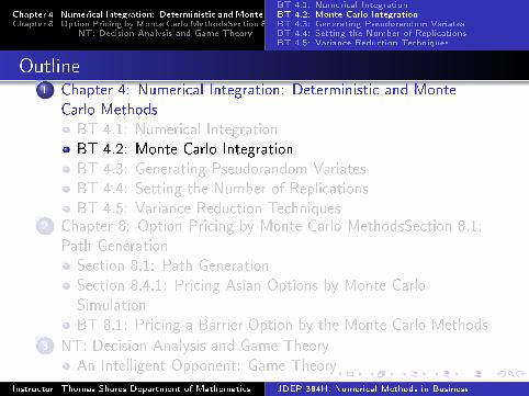
Outline1 Chapter 4: Numerical Integration: Deterministic and Monte

Carlo MethodsBT 4.1: Numerical IntegrationBT 4.2: Monte Carlo IntegrationBT 4.3: Generating Pseudorandom VariatesBT 4.4: Setting the Number of ReplicationsBT 4.5: Variance Reduction Techniques

2 Chapter 8: Option Pricing by Monte Carlo MethodsSection 8.1:Path GenerationSection 8.1: Path GenerationSection 8.4.1: Pricing Asian Options by Monte CarloSimulationBT 8.1: Pricing a Barrier Option by the Monte Carlo Methods

3 NT: Decision Analysis and Game TheoryAn Intelligent Opponent: Game Theory




BT 4.1: Numerical IntegrationBT 4.2: Monte Carlo IntegrationBT 4.3: Generating Pseudorandom VariatesBT 4.4: Setting the Number of ReplicationsBT 4.5: Variance Reduction Techniques








































Section 8.1: Path GenerationSection 8.4.1: Pricing Asian Options by Monte Carlo SimulationBT 8.1: Pricing a Barrier Option by the Monte Carlo Methods








3 NT: Decision Analysis and Game TheoryAn Intelligent Opponent: Game TheoryInstructor: Thomas Shores Department of Mathematics JDEP 384H: Numerical Methods in Business









De�nition of An Asian Option:

Here is one type of Asian (call) option, where a daily average of thestock is computed over the life of the option. Instead of using priceS(T ) of the option, one uses the average value of the option in thepayo� formula.

Result: the payo� curve gives

fT = max

{0,

1

N

N∑i=1

S (ti )− K

}where K is the strike price

and T consists of N days.

Thus the actual path of a particular daily history of the stockprice in�uences the payo� and hence the price of the option.To estimate the price f discount the average of the computedvalues fT over various stock paths.

Control variates can be helpful. Use C =N∑i=1

S (ti ) as control.

Compute expected value by discounting each term to expiry T .




fT = max

{0,

1

N

N∑i=1

S (ti )− K





S (ti ) as control.





fT = max

{0,

1

N

N∑i=1

S (ti )− K





S (ti ) as control.





fT = max

{0,

1

N

N∑i=1

S (ti )− K





S (ti ) as control.


Example Calculations

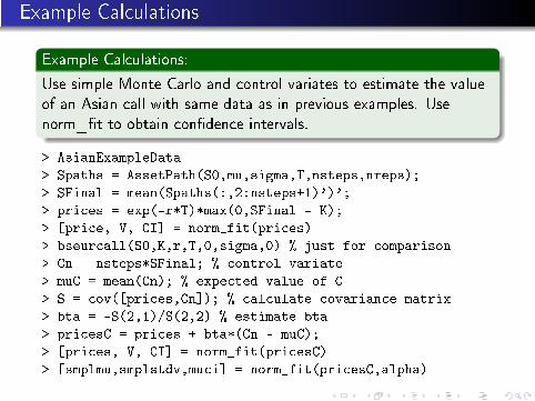
Example Calculations:

Use simple Monte Carlo and control variates to estimate the valueof an Asian call with same data as in previous examples. Usenorm_�t to obtain con�dence intervals.

> AsianExampleData

> Spaths = AssetPath(S0,mu,sigma,T,nsteps,nreps);

> SFinal = mean(Spaths(:,2:nsteps+1)')';

> prices = exp(-r*T)*max(0,SFinal - K);

> [price, V, CI] = norm_fit(prices)

> bseurcall(S0,K,r,T,0,sigma,0) % just for comparison

> Cn = nsteps*SFinal; % control variate

> muC = mean(Cn); % expected value of C

> S = cov([prices,Cn]); % calculate covariance matrix

> bta = -S(2,1)/S(2,2) % estimate bta

> pricesC = prices + bta*(Cn - muC);

> [prices, V, CI] = norm_fit(pricesC)

> [smplmu,smplstdv,muci] = norm_fit(pricesC,alpha)












Barrier Options

What They Are:

Option in which there is an agreed barrier Sb, which may or maynot be reached by the price S of the stock in question.

Knock-out option: contract is voided if the barrier value isreached at any time during the whole life of option.

Knock-in option: option is activated only if the barrier isreached.

S > Sb: a down option.

S < Sb: an up option.

Analytic formulas are known for certain barrier options,including a down-and-out put.





Barrier Options

What They Are:











Barrier Options

What They Are:











Barrier Options

What They Are:











Barrier Options

What They Are:











Barrier Options

What They Are:








Pricing a Barrier Option by Monte Carlo Methods

How It's Done:

Given a random walk of S of length N with S (tN) = T , thepayo� curve gives fT = max {0, (S (tN)− K ) I (S)} where K isthe strike price and the indicator function I (S) is zero if anyS (tj) < Sb and one otherwise.

Of course, fT is a r.v. But the drift for this asset should be therisk-free rate r . So all we have to do is average the payo�sover various stock price paths to time T , then discount theaverage to obtain an approximation for f0.


How It's Done:




How It's Done:



Example Calculations

Example Calculations:

Use simple Monte Carlo to estimate the value of a down-and-output with same data as in previous examples and Sb = 80. Usenorm_�t to obtain con�dence intervals.

> Sb = 80

> truemean = DownOutPut(S0,K,r,T,0,sigma,Sb)

> bseurput(S0,K,r,T,0,sigma,0) % just for comparison

> randn('state',0)

> Spaths = AssetPath(S0,mu,sigma,T,nsteps,nreps);

> SFinal = Spaths(:,nsteps+1);

> Indicator = (sum((Spaths<Sb)')')==0;

> prices = exp(-r*T)*max(0,(K-SFinal).*Indicator);

> [smplmu,smplvar,muci,varci] = norm_fit(prices,alpha)

> % now lower the barrier and see what happens


NT: Decision Analysis and Game TheoryAn Intelligent Opponent: Game Theory








A Model Problem

Business Competition as a Game:

Two companies compete for the bulk of a shared market for acertain product and plan to execute one of three strategies. Bothmarketing departments analyzed them and have arrived atessentially the same �gures for outcomes.

The three strategies are:

Better packaging.An advertising campaign.Slight price reduction.

We assume:

Payo�s for this competition (game) are known to all.Players are rational players who play to win.Neither side has advance knowledge of the opponent's play.Whatever one side gains, the other loses (zero-sum game.)




A Model Problem





We assume:





A Model Problem





We assume:



The Numbers

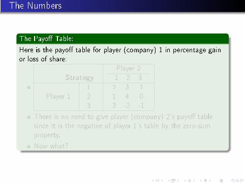
The Payo� Table:

Here is the payo� table for player (company) 1 in percentage gainor loss of share:

Strategy

Player 2

1 2 3

Player 1123

2 3 11 4 03 -2 -1

There is no need to give player (company) 2's payo� tablesince it is the negative of player 1's table by the zero-sumproperty.

Now what?

The Numbers

The Payo� Table:


Strategy

Player 2

1 2 3

Player 1123

2 3 11 4 03 -2 -1


Now what?

The Numbers

The Payo� Table:


Strategy

Player 2

1 2 3

Player 1123

2 3 11 4 03 -2 -1


Now what?

The Numbers

The Payo� Table:


Strategy

Player 2

1 2 3

Player 1123

2 3 11 4 03 -2 -1


Now what?

Stragegies

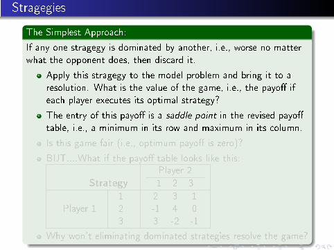
The Simplest Approach:

If any one stragegy is dominated by another, i.e., worse no matterwhat the opponent does, then discard it.

Apply this stragegy to the model problem and bring it to aresolution. What is the value of the game, i.e., the payo� ifeach player executes its optimal strategy?

The entry of this payo� is a saddle point in the revised payo�table, i.e., a minimum in its row and maximum in its column.

Is this game fair (i.e., optimum payo� is zero)?

BUT....What if the payo� table looks like this:

Strategy

Player 2

1 2 3

Player 1123

2 3 1-1 4 03 -2 -1

Why won't eliminating dominated strategies resolve the game?

Stragegies







Strategy

Player 2

1 2 3

Player 1123

2 3 1-1 4 03 -2 -1


Stragegies







Strategy

Player 2

1 2 3

Player 1123

2 3 1-1 4 03 -2 -1


Stragegies







Strategy

Player 2

1 2 3

Player 1123

2 3 1-1 4 03 -2 -1


Stragegies







Strategy

Player 2

1 2 3

Player 1123

2 3 1-1 4 03 -2 -1


Stragegies







Strategy

Player 2

1 2 3

Player 1123

2 3 1-1 4 03 -2 -1


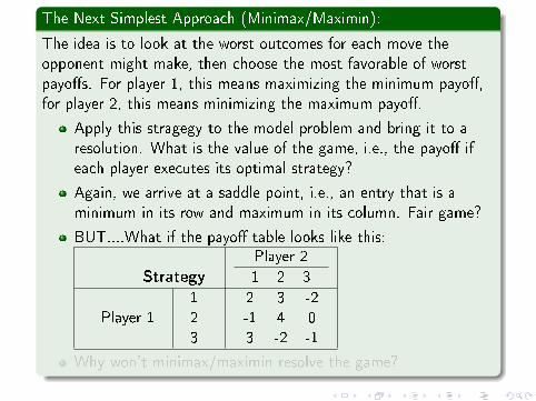
The Next Simplest Approach (Minimax/Maximin):

The idea is to look at the worst outcomes for each move theopponent might make, then choose the most favorable of worstpayo�s. For player 1, this means maximizing the minimum payo�,for player 2, this means minimizing the maximum payo�.


Again, we arrive at a saddle point, i.e., an entry that is aminimum in its row and maximum in its column. Fair game?


Strategy

Player 2

1 2 3

Player 1123

2 3 -2-1 4 03 -2 -1

Why won't minimax/maximin resolve the game?






Strategy

Player 2

1 2 3

Player 1123

2 3 -2-1 4 03 -2 -1







Strategy

Player 2

1 2 3

Player 1123

2 3 -2-1 4 03 -2 -1







Strategy

Player 2

1 2 3

Player 1123

2 3 -2-1 4 03 -2 -1







Strategy

Player 2

1 2 3

Player 1123

2 3 -2-1 4 03 -2 -1


Stragegies

The Least Simple Approach:

Use mixed strategies instead of pure strategies, i.e., a probabilityvector (x1, x2, x3) for player 1 (y = (y1, y2, y3) for player 2) thatmaximizes (minimizes) the payo� for all possible plays by theopponent.

If the payo� table is converted into a matrix A (m × n ingeneral), then the payo� for any pair of mixed strategies is

p = Σmi=1Σ

nj=1aijxiyj = xTAy

Player 1's goal: Find probability vector x solvingmaxx

miny

xTAy.

Player 2's goal: Find probability vector y solvingminy

maxx

xTAy.

Stragegies




p = Σmi=1Σ

nj=1aijxiyj = xTAy


miny

xTAy.


maxx

xTAy.

Stragegies




p = Σmi=1Σ

nj=1aijxiyj = xTAy


miny

xTAy.


maxx

xTAy.

Stragegies




p = Σmi=1Σ

nj=1aijxiyj = xTAy


miny

xTAy.


maxx

xTAy.

Documents

JDEP 384H: Numerical Methods in Business - …tshores1/Public/JDEP384... · BT 8.1: Pricing a Barrier Option yb the Monte Carlo Methods Instructor: Thomas Shores Department of Mathematics