MEMORANDUM

UNITED STATES ENVIRONMENTAL PROTECTION AGENCY

RESEARCH TRIANGLE PARK, NC 27711

JAN Z Z 2015 OFFICE OF AIR QUALITY PLANNING

AND STANDARDS

SUBJECT: Information on the Interstate Transport "Good Neighbor" Provision for the 2008 Ozone National Ambient Air Quality Standards (NAAQS) under Clean Air Act (CAA) Section 110(a)(2)(D)(i )

FROM: Stephen D. Pag Director

TO: Regional Air Division Directors, Regions 1 - 10

The purpose of this memorandum is to provide information to states regarding state implementation plans (SIPs) to address the interstate transport "Good Neighbor" Provision of the Clean Air Act (CAA) as it pertains to the 2008 ozone National Ambient Air Quality Standards (NAAQS). This information consists of:

• Discussion of elements that have been used previously to address interstate transport, and • The EPA' s preliminary air quality modeling data for ozone for the year 2018.

The EPA anticipates that this information, together with additional steps described below, will be helpful to states developing "Good Neighbor" SIPs for the 2008 ozone NAAQS. The EPA and states are behind schedule in addressing the "Good Neighbor" Provision for the 2008 ozone standards, due to factors such as the EPA' s reconsideration of the standards and protracted litigation related to previous actions [most recently the Cross-State Air Pollution Rule (CSAPR)] under the "Good Neighbor" Provision. This document is part of the process of working with states to offer support and information to enable the EPA and states to move forward to address the requirements of the "Good Neighbor" Provision for this NAAQS as soon as possible.

In addition to the information being shared today, the EPA will hold a webinar in early February and a workshop in the spring of2015. The webinar will focus on the content of this memo and the attached preliminary air quality modeling data. For the workshop, the EPA plans to facilitate discussions with states on: (1) available emission controls; (2) potential state-by-state electric generating unit (EGU) nitrogen oxides (NOx) reductions based on those controls; and (3) potential EGU emissions budgets informed by those reductions. More information on the webinar and workshop will be forthcoming.

The EPA's goal is to provide information and to initiate discussions that will inform state development and EPA review of "Good Neighbor" SIPs, and, where appropriate, to facilitate state efforts to supplement or resubmit their "Good Neighbor" SIPs. At this time, there are a number of states that may not have submitted "Good Neighbor" SIPs for the 2008 ozone NAAQS. In addition, there are a number

Internet Address (URL) • http://www.epa.gov Recycled/Recyclable •Printed with Vegetable 011 Based Inks on Recycled Paper (Minimum 25% Postconsumer)

of pending "Good Neighbor" SIPs for the 2008 ozone NAAQS that the EPA will review and take action on. While our goal is to facilitate SIP development, the EPA also recognizes its backstop role in the SIP development process-that is, our obligation to develop and promulgate federal imp~ementation plans, as appropriate. We plan to take this action, if necessary. It is our intention that any federal rule developed to satisfy this obligation would provide ample opportunity for states to pursue alternatives.

The "Good Neighbor" Provision

Under CAA sections 1 IO(a)(l) and 110(a)(2), each state1 is required to submit a SIP2 that provides for the implementation, maintenance and enforcement of each primary or secondary NAAQS. Moreover, section 11 O(a)(l) requires each state to make this new SIP submission within 3 years after promulgation of a new or revised NAAQS. 3 This type of SIP submission is commonly referred to as an "infrastructure SIP." The conceptual purpose of an infrastructure SIP submission is to assure that the state's SIP contains the necessary structural requirements for the implementation of the new or revised NAAQS, whether by establishing that the SIP already contains or sufficiently addresses the necessary provisions, or by making a substantive SIP revision to update the SIP.

CAA section 110(a)(2)(D)(i)(I) requires each state in its SIP to prohibit emissions that will significantly contribute to nonattainment of a NAAQS, or interfere with maintenance of a NAAQS, in a downwind state. Under section 110( a)(2)(D)(i)(I), each state is required to submit to the EPA new or revised SIPs that "contain adequate provisions - prohibiting, consistent with the provisions of this subchapter, any source or other type of emissions activity within the state from emitting any air pollutant in amounts which will . .. contribute significantly to nonattainment in, or interfere with maintenance by, any other state with respect to any such national primary or secondary ambient air quality standard." For purposes of this document, we refer to section 110(a)(2)(D)(i)(I) as the "Good Neighbor Provision" and to SIP revisions addressing this requirement as "Good Neighbor SIPs."

Elements That Have Been Used Previously to Address the' Good Neighbor" Provision

The EPA notes that a consistent framework for addressing transport for certain NAAQS, involving a number of basic steps, has been developed in several previous federal rulemakings.4 These basic steps include: (1) identifying downwind air quality problems, (2) identifying upwind states that contribute enough to those downwind air quality problems to warrant further review and analysis, (3) identifying

1 The term "state" as used in this memorandum has the same meaning as provided in CAA section 302(d). These CAA sections and this information may also apply, as appropriate under the Tribal Authority Rule (TAR) in 40 CFR part 49, to an Indian tribe that receives a determination of eligibility for treatment in a similar manner as a state for purposes of administering a tribal air quality management program under section 1 lO(a}l>fthe CAA. Tribes should look to the TAR and engage their respective EPA regional offices in discussing how this information may impact the development and approvability of their tribal implementation plans (TIPs). We encourage states to provide outreach and engage in discussions with tribes about their SIPs as they are being developed. · 2 In the CAA and in this memorandum, "plan," "SIP" and "TIP" may, depending on context, refer either to (i) all or part of the existing state (or tribal) implementation plan (i.e., the collection of all submissions previously approved by the EPA as meeting CAA requirements) or (ii) a submission that adds to or modifies the existing plan as directed by section l lO(a)(l). 3 The Administrator may specify a shorter period. 4 See for example, Finding of Significant Contribution and Rulemaking for Certain States in the Ozone Transport Assessment Group Region for Purposes of Reducing Regional Transport of Ozone. 63 FR 57356 (October 27, 1998); Clean Air Interstate Rule (CAIR) Final Rule. 70 FR 25162 (May 12, 2005); CSAPR Final Rule. 76 FR 48208 (August 8, 2011).

2

the emissions reductions necessary to prevent an identified upwind state from contributing significantly to those downwind air quality problems and ( 4) adoption of permanent and enforceable measures needed to achieve those emissions reductions.

Efforts to address ozone transport by the EPA and states under the "Good Neighbor" Provision have focused on reductions of NOx as the precursor pollutant for which emissions in upwind states have the greatest impacts on transported ozone. 5

In CSAPR, downwind air quality problems were assessed based on modeled future air quality concentrations for a year aligned with attainment deadlines for a particular NAAQS. The assessment of future air quality conditions generally accounted for on-the-books emissions reductions6 and the most up-to-date forecast of future baseline emissions. The locations of downwind air quality problems were identified as those receptors that were projected to be unable to attain or maintain the standard. More detail on the methods for identifying problem receptors in CSAPR is contained in the attachment.

CSAPR used a screening threshold (1 percent of the NAAQS) to identify contributing upwind states warranting further review and analysis. States whose air quality impact7 to at least one downwind problem receptor was greater than or equal to the threshold were identified as needing further evaluation for actions to address transport. States whose air quality impacts to all downwind problem receptors were below this threshold were identified as states not requiring further evaluation for actions to address transport-that is, these states had no emissions reduction obligation under the "Good Neighbor" Provision.

In order to quantify emissions reductions needed to eliminate significant contributions to a downwind air quality problem, CSAPR's apportionment ofresponsibility evaluated air quality and included consideration of cost, an approach that was recently upheld by the U.S. Supreme Court. 8 The selection of cost criteria was informed by air quality considerations. For example, the approach in CSAPR for sulfur dioxide contributions to fine particulate matter (PM2.s) placed states into two groups based on differing air quality considerations at downwind receptors. For states within each group, however, a uniform cost level was used to determine needed emissions reductions.

The EPA's preliminary air quality modeling analysis (see attachment and the Air Quality Modeling Technical Support Document for the 2008 Ozone NAAQS Transport Assessment located at www.epa.gov/airtransport) applies the CSAPR approach to the 2008 ozone NAAQS, including the approach for identifying nonattainment and maintenance receptors and for identifying upwind states that contribute to these receptors based on the 1 percent screening threshold. Following the CSAPR approach, a state could either demonstrate that its contribution is below the screening threshold, or it could evaluate the scope of its transport obligation and identify measures to achieve any needed emissions reductions. The discussions at the spring 2015 workshop are intended to help states with their evaluation of such emissions reductions.

5 See discussion in preamble to the CSAPR Final Rule. 76 FR 48222 (August 8, 2011). 6 The exception being CAIR, which CSAPR was designed to replace and therefore was not considered on-the-books. 7 For ozone the impacts would include those from volatile organic compounds (VOC) and NOx, and from all sectors. 8 EPA v. EME Homer City Generation, L.P., 134 S. Ct. 1584, 1606-07 (2014).

3

CSAPR and its predecessor transport rules, the NOx SIP Call and CAIR, were designed to address the collective contributions from the 37 states in the Eastern U.S. and were not formally evaluated for applicability to the 11 states in the Western U.S.9 The EPA's preliminary modeling indicates that most western states contribute less than 1 percent to downwind nonattainment or maintenance receptors, a level the EPA considered to not need further evaluation for actions to address transport in CSAPR. There are a few receptors in the West where 1 to 3 western states may contribute amounts potentially exceeding the 1 percent threshold (See Technical Support Document). Due to the possibility that additional considerations may impact the EPA's and state's evaluation of transport from these potentially linked states in the Western U.S., we expect that the EPA and states will continue to evaluate these western transport linkages (not included in the attachment) on a case-by-case basis. We recommend that states consult with their EPA regional offices regarding these specific situations.

For Further Information

If you have any questions concerning this information, please contact Tim Smith, at (919) 541-4718, smith.tim@epa.gov, or Gobeail McKinley, at (919) 541-5246, mckinley.gobeail@epa.gov.

Attachment

9 For the purposes of this information document, we include the 37 states and the District of Columbia in the region from Texas northward to North Dakota and eastward to the East Coast as comprising the Eastern U.S. The Western U.S. refers to the 11 states in the contiguous U.S. west of those states (AZ, CA, CO, ID, MT, NM, NV, OR, UT, WA and WY).

4

Attachment

Air Quality Modeling Results

A. Background

The EPA performed photochemical air quality modeling to project ozone concentrations at air

quality monitoring sites to 2018, the moderate area attainment date for the 2008 ozone National Ambient

Air Quality Standards (NAAQS), and to estimate state-by-state contributions to those 2018

concentrations. We then used the air quality modeling results, and the methods we used for Cross-State

Air Pollution Rule (CSAPR), to identify ozone monitoring sites expected to be nonattainment or

maintenance receptors for the 2008 ozone NAAQS in 2018. We used the contribution information to

quantify projected interstate contributions from emissions in each upwind state to ozone concentrations

at each identified 2018 nonattainment and maintenance receptor in downwind states. The EPA' s air

quality modeling used the 2011-based air quality modeling platform. This platform includes emissions

for a 2011 base year and a 2018 future base case as well as meteorology for 2011. The 2011

meteorology was used in air quality model simulations for both 2011 and 2018. We selected 2011 as the

base year because it reflected the most current National Emissions Inventory (NEI) available. Details on

the construct and evaluation of the 2011-based air quality modeling platform are provided in the Air

Quality Modeling Technical Support Document for the 2008 Ozone NAAQS Transport Assessment

(AQMTSD).

The 2011 base year emissions in the 2011-based air quality modeling platform were derived

from the 2011 NEI, as described in the Technical Support Document: Preparation of Emissions

Inventories for the Version 6.0, 2011 Emissions Modeling Platform. 10 This document also describes the

control and growth assumptions by source type that were used to create the 2018 base case emissions

inventory. 11 The EPA released the 2011 and 2018 emissions inventory for public review on

10 Available on the EPA's website at: http://www.epa.gov/ttnchiel/emch. 11 For electric generating units (EGUs), the 2018 base case emissions were obtained from the Integrated Planning Model (IPM version 5.13, http://www.epa.gov/powersectormodeling/BaseCasev513. html). The 2018 base case EGU projections include the Acid Rain Program, Clean Air Interstate Rule (CAIR), and Mercury and Air Toxics Standards. The base case does not include CSAPR, the proposed Clean Power Plan or the proposed 2015 ozone NAAQS, because of the time the projections were developed.

1

November 27, 2013 (78 FR 70935), and January 14, 2014 (79 FR 2437), respectively. The air quality

modeling presented in this transport information document pre-dated, and therefore does not reflect,

comments received from this public review process of the 2011 and 2018 emissions inventories. We

note that the EPA plans to re-model 2011and2018 to provide updated projections of2018 design values

and contributions, using revised inventories created in response to comments on this public review

process and other emissions updates.

The EPA used the Comprehensive Air Quality Model with Extensions (CAMx version 6.10)12

for modeling the 2011 base year and 2018 base case emissions scenarios to identify sites with projected

nonattainment and maintenance problems in 2018. As shown in Figure 1, the air quality model runs

were performed for a modeling domain that covers the 48 states in the contiguous U.S. along with

adjacent portions of Canada and Mexico. The spatial resolution (i.e., grid size) for this modeling domain

is 12 km x 12 km. The 2011 and 2018 scenarios were also both modeled for the full year with 2011

meteorology.

12 Environ, April 4, 2014 (http://www.camx.com).

2

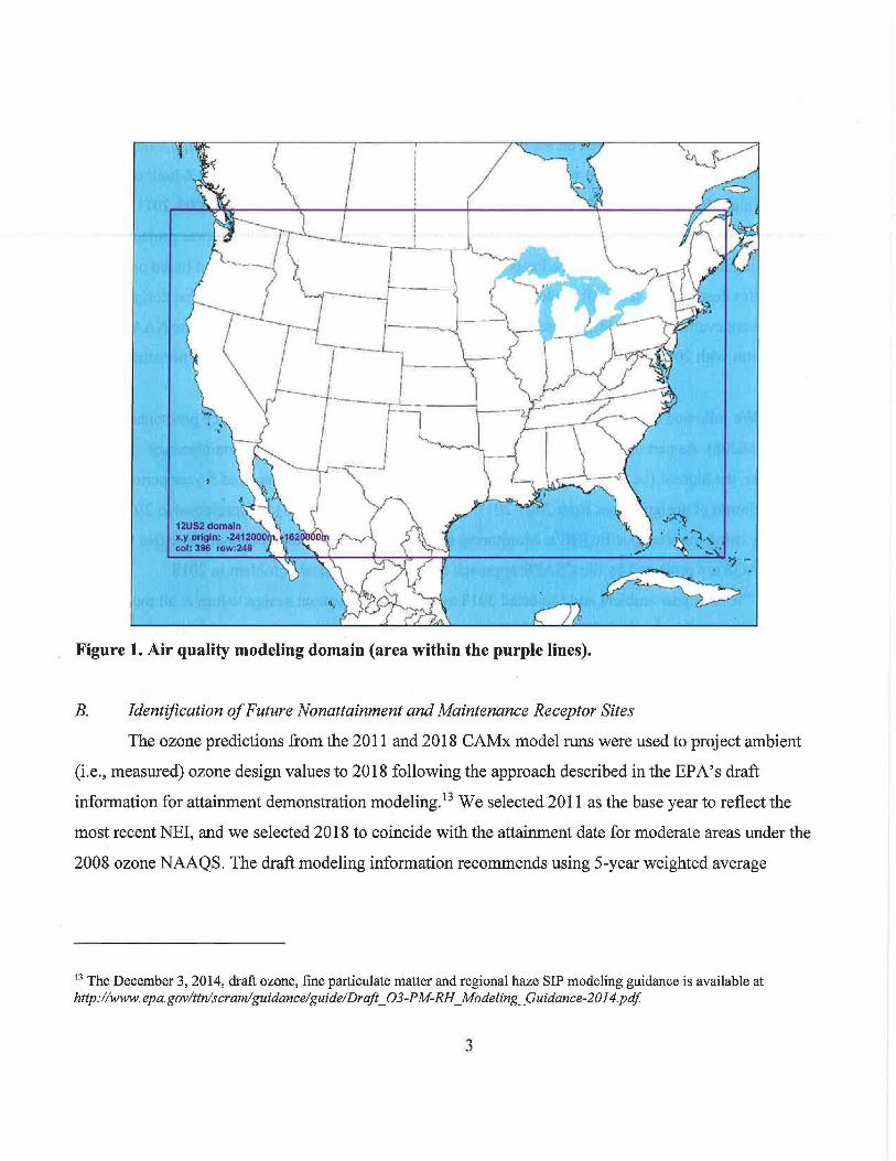
Figure 1. Air quality modeling domain (area within the purple lines).

B. Identification of Future Nonattainment and Maintenance Receptor Sites

~ : . ")_,

..... .. ... . .,, -

The ozone predictions from the 2011and2018 CAMx model runs were used to project ambient

(i.e., measured) ozone design values to 2018 following the approach described in the EPA' s draft

information for attainment demonstration modeling. 13 We selected 2011 as the base year to reflect the

most recent NEI, and we selected 2018 to coincide with the attainment date for moderate areas under the

2008 ozone NAAQS. The draft modeling information recommends using 5-year weighted average

13 The December 3, 2014, draft ozone, fine particulate matter and regional haze SIP modeling guidance is available at http://www.epa.gov/ttnlscramlguidance/guide/Draft _ 03-P M-RH _Modeling_ Guidance-2014.pdf

3

ambient design values14 centered on the base year as the starting point for projecting design values to the

future. Because 2011 is the base year of emissions, we started with the average ambient 8-hour ozone

design values for the period 2009 through 2013 (i.e., the average of design values for 2009-2011, 2010-

2012 and 2011-2013). The 5-year weighted average ambient design value at each site was projected to

2018 using model-predicted Relative Response Factors (RRFs) 15 which were calculated based on

procedures described in the draft modeling information. The 2018 projected average ozone design

values were evaluated to identify those sites with design values that exceed the 2008 ozone NAAQS. 16

Those sites with 2018 average design values that exceed the NAAQS are projected to be nonattainment

in 2018.

We followed the CS APR approach to identify sites with projected maintenance problems in 2018

(76 FR 48208). As part of the approach for identifying sites with projected future maintenance

problems, the highest (i.e., maximum) ambient design value from the 2011-centered 5-year period (i.e.,

the maximum of design values from 2009-2011, 2010-2012 and 2011-2013) was projected to 2018 for

each site using the site-specific RRFs. Monitoring sites with a 2018 maximum design value that exceeds

the NAAQS are projected by the CSAPR approach to have a maintenance problem in 2018.

The base year ambient and projected 2018 average and maximum design values at all monitoring

sites are provided in the AQMTSD. In 2018 there are 11 projected nonattainment sites and 18 projected

maintenance sites in the East (See Table 1). These are the sites that are indicated from the EPA's

preliminary modeling as warranting the evaluation of contributions from upwind states. T?e projected

2018 nonattainment sites in the East are located in four nonattainment areas: Baltimore, MD; New York

City, NY (sites in both NY and CT); Dallas, TX; and Houston, TX. Note that several of these

nonattainment areas also contain additional sites that are projected as maintenance receptors. Also, there

are several projected maintenance-only areas in the East: Holland, MI; Louisville, KY; Philadelphia, PA

(including sites in both NJ and PA); St. Louis, MO; and Sheboygan, WI (See Table 2).

14 The air quality design value for a site is the 3-year average annual fourth-highest daily maximum 8-hour average ozone concentration. 15 In brief, the RRF for a particular location is the ratio of the 2018 ozone model prediction to the 2011 ozone model prediction. The RRFs were calculated using model outputs for the May through September period. 16 In determining compliance with the NAAQS, ozone design values are truncated to integer values. For example, a design value of75.9 ppb is truncated to 75 ppb which is attainment. In this manner, design values at or above 76.0 ppb are considered nonattainment.

4

Table 1. Ambient and 2018 projected average and maximum 8-hour ozone design values (DVs) at 2018 nonattainment receptors in the East (nonattainment receptors have a 2018 average design value of:=: 76.0 ppb). Units are ppb.

2009- 2009-2013Avg 2013 Max 2018Avg 2018 Max

State County Site ID DVs DVs DVs DVs

Connecticut Fairfield 90013007 84.3 89.0 76.7 81.0

Connecticut Fairfield 90019003 83.7 87.0 77.5 80.6

Marv land Harford 240251001 90.0 93.0 79.4 82.1

New York Suffolk 361030002 83.3 85.0 78.2 79.8

Texas Brazoria 480391004 88.0 89.0 80.5 81.4

Texas Denton 481210034 84.3 87.0 77.0 79.5

Texas Harris 482010024 80.3 83.0 76.4 79.0

Texas Harris 482011034 81.0 82.0 76.6 77.6

Texas Harris 4820 11039 82.0 84.0 77.7 79.6

Texas Tarrant 484392003 87.3 90.0 79.7 82.2

Texas Tarrant 484393009 86.0 86.0 78.3 78.3

Table 2. Ambient and 2018 projected average and maximum 8-hour ozone design values (DVs) at 2018 maintenance receptors in the East (maintenance receptors have a 2018 maximum design value of:=: 76.0 ppb). Units are ppb.

2009- 2009-2013 Avg 2013 Max 2018 Avg 2018 Max

State County Site ID DVs DVs DVs DVs

Connecticut Fairfield 90010017 80.3 83.0 74.1 76.6

Connecticut New Haven 90099002 85.7 89.0 75.8 78.8

Kentuckv Jefferson 211110067 82.0 85.0 73 .7 76.4

Michigan Allegan 260050003 82.7 86.0 74.5 77.5

Missouri Saint Charles 291831002 82.3 86.0 74.1 77.4

New Jersey Camden 340071001 82.7 87.0 72.3 76.0

New Jersey Gloucester 340150002 84.3 87.0 74.0 76.3

New York Richmond 360850067 81.3 83.0 74.6 76.2

Pennsylvania Philadelphia 421010024 83.3 87.0 74.7 78.0

Texas Collin 480850005 82.7 84.0 75.0 76.2

Texas Dallas 481130069 79.7 84.0 73.7 77.7

Texas Dallas 481130075 82.0 83.0 75.2 76.I

Texas Denton 481211032 82.7 84.0 75.1 76.3

5

2009 - 2009 -2013 Avg 2013 Max 2018 Avg 2018 Max

State County Site ID DVs DVs DVs DVs

Texas Harris 482010029 83.0 84.0 75.4 76.3

Texas Harris 482010055 81.3 83.0 75.0 76.6

Texas Tarrant 484390075 82.0 83.0 75.5 76.4

Texas Tarrant 484393011 80.7 83.0 74.2 76.3

Wisconsin Sheboygan 551170006 84.3 87.0 75.4 77.8

C. Quantification of Interstate Ozone Contributions

The EPA performed nationwide,17 state-level ozone source apportionment modeling using the

CAMx Ozone Source Apportionment Technology/ Anthropogenic Precursor Culpability Analysis

(OSAT/APCA) technique18 to quantify the contribution of2018 base case nitrogen oxides (NOx) and

volatile organic compound (VOC) emissions from all sources in each state to projected 2018 ozone

concentrations at air quality monitoring sites. In the source apportionment model run, we tracked the

ozone formed from each of the following contribution categories (i.e., "tags"):

• States - anthropogenic NOx and VOC emissions from each state tracked individually (emissions

from all anthropogenic sectors in a given state were combined),

• Biogenics - biogenic NOx and VOC emissions domainwide (i.e. , not by state),

• Boundary Concentrations - concentrations transported into the nationwide modeling domain,

• Tribes - the aggregate of emissions from those tribal lands for which we have point source

inventory data in the 2011 NEI (i.e., we did not model the contributions from individual tribes),

and

• Other - combined emissions from wild and prescribed fires, offshore emissions from marine

vessels, offshore drilling platforms and anthropogenic emissions from the portions of Canada

and Mexico within the modeling domain.

17 As shown in Figure I, the EPA's nationwide modeling includes the 48 contiguous states. 18 As part of this technique, ozone formed from reactions between biogenic voe and NOx with anthropogenic NOx and voe are assigned to the anthropogenic emissions.

6

The CAMx OSAT/APCA model run was performed for the period May 1 through September 30

using the projected 2018 base case emissions and 2011 meteorology for this time period. The hourly

contributions19 from each tag were processed to obtain the 8-hour average contributions corresponding

to the time period of the 8-hour daily maximum concentration on each day in the 2018 model

simulation. This step was performed for those model grid cells containing monitoring sites in order to

obtain 8-hour average contributions for each day at the location of each site. The model-predicted

contributions were then applied in a relative sense to quantify the contributions to the 2018 average

design value at each site. First, the daily 8-hour contributions were averaged across the subset of days

with 2018 model predictions exceeding the 2008 ozone NAAQS (i.e., 8-hr daily maximum~ 76 ppb).

For those sites with fewer than 5 predicted exceedance days in 2018, we averaged the contributions for

the top five concentrations days.2° For each site, the multi-day average contribution from each tag was

normalized by the sum of the contribution from all tags, combined. The resulting fractional contributions

at each site were then applied to the 2018 average design value to quantify (i.e., "apportion") the design

value into contributions from each tag. This process was performed for each monitoring site with a

projected 2018 design value. Additional details on the source apportionment modeling and the

calculation of contributions can be found in the AQMTSD. The resulting 2018 contributions from each

tag to each monitoring site are provided in the AQMTSD. The largest contributions from each state to

2018 downwind nonattainment receptors and to downwind maintenance receptors are provided in

Table 3.

19 Contributions from anthropogenic emissions under "NOx-limited" and "VOC-limited" chemical regimes were combined to obtain the net contribution from NOx and VOC anthropogenic emissions in each state. 20 If a site did not have at least 5 days with a modeled 2018 8-hour daily maximum concentration:::: 60 ppb, then contributions were not calculated at the monitor.

7

Table 3. Largest ozone contributions from each state to downwind 2018 projected nonattainment and to 2018 projected maintenance receptors. Units are ppb.

Largest Contribution to Largest Contribution to a 2018 Nonattainment a 2018 Maintenance

Site in Downwind Site in Downwind Upwind State States States

Alabama 1.06 1.39 Arizona l.47a 0.44 Arkansas 1.25 2.19 California 0.23 1.16a Colorado 0.35 0.33 Connecticut 0.41 0.08 Delaware 0.63 2.46 District of Columbia 0.69 0.29 Florida 0.87 1.05 Georgia 0.71 0.73 Idaho 0.09 0.22 Illinois 0.87 22.29 Indiana 1.93 11.41 Iowa 0.62 0.89 Kansas 0.70 1.15 Kentucky 1.94 2.40 Louisiana 3.38 4.37 Maine 0.01 0.00 Maryland 2.59 6.96 Massachusetts 0.21 0.12 Michigan 1.48 3.63 Minnesota 0.43 0.34 Mississippi 0.83 1.52 Missouri 1.53 4.12 Montana 0.14 0.17 Nebraska 0.36 0.56 Nevada 0.70 0.44 New Hampshire 0.03 0.02 New Jersey 9.21 9.95 New Mexico 0.26 0.20 New York 16.05 16.14 North Carolina 0.57 0.55 North Dakota 0.13 0.19 Ohio 4.06 4.41 Oklahoma 1.50 2.59 Oregon 0.69 0.73 Pennsylvania 9.85 18.76 Rhode Island 0.04 0.03

8

Largest Contribution to Largest Contribution to a 2018 Nonattainment a 2018 Maintenance

Site in Downwind Site in Downwind Upwind State States States

South Carolina 0.36 0.35 South Dakota 0.09 0.12 Tennessee 0.69 0.99 Texas 0.92 2.74 Utah 0.29 l.43a Vermont 0.02 0.02 Virginia 4.42 3.27 Washington 0.21 0.13 West Virginia 2.79 2.88 Wisconsin 0.34 2.49 Wyoming 0.37 l.29a

a These four western states (i.e., AZ, CA, UT, and WY) contribute above the 1 percent threshold to projected 2018 nonattainment or maintenance sites in the West, as identified in the AQMTSD.

Table 4 indicates the projected state "linkages" to downwind 2018 nonattainment receptors in the

Eastern U.S.21 identified in the air quality modeling using a threshold of 1 percent of the 2008 ozone

NAAQS (0.76 ppb), consistent with CSAPR. Table 5 provides the same information for states that

contribute at or above the 1 percent threshold to identified 2018 maintenance receptors in the Eastern

U.S. (States in the Eastern U.S. that are not listed in these tables contribute below 1 percent at all

receptors).

21 For the purposes of this information document, we include the 37 states and the District of Columbia in the region from Texas northward to North Dakota and eastward to the East Coast as comprising the Eastern U.S. The Western U.S. refers to the 11 states in the contiguous U.S. west of those states (AZ, CA, CO, ID, MT, NM, NV, OR, UT, WA and WY).

9

Table 4. Ozone contributions at or above a 1 percent threshold from upwind states to 2018 nonattainment receptors in the Eastern U.S. Units are ppb.

2018 N onattainment Upwind States - Part 1 (AL through MS)

Receptors County Site ID AL AR FL IL IN KY LA MD MI MS

Fairfield, CT 90013007 2.11 0.93 Fairfield, CT 90019003 2.60 Harford, MD 240251001 1.93 1.95 0.86 Suffolk, NY 361030002 0.79 1.02 1.50 1.49 Brazoria, TX 480391004 1.00 0.88 3.25 0.81 Denton, TX 481210034 1.06 0.95 3.13 Harris, TX 482010024 0.87 2.24 Harris, TX 482011034 1.06 0.81 3.39 Harris, TX 482011039 1.25 2.93 0.84 Tarrant, TX 484392003 0.82 0.97 2.94 Tarrant, TX 484393009 1.19 2.29

Number of Linkages=> 2 6 1 3 2 1 7 3 3 2

2018 Nonattainment Upwind States - Part 2 (MO through WV)

Receptors County Site ID MO NJ NY OH OK PA TX VA WV

Fairfield, CT 90013007 6.72 15.58 1.92 9.86 1.92 0.97 Fairfield, CT 90019003 8.17 16.06 1.50 9.30 2.17 0.89 Harford, MD 240251001 4.07 6.93 0.92 4.43 2.80 Suffolk, NY 361030002 9.21 2.52 9.79 0.80 1.72 0.99 Brazoria, TX 480391004 1.20 0.77 Denton, TX 481210034 1.12 Harris, TX 482010024 Harris, TX 482011034 1.53 1.51 Harris, TX 482011039 1.06 0.99 Tarrant, TX 484392003 1.22 Tarrant, TX 484393009 1.25

Number of Linkages => 3 3 2 4 6 4 2 4 4

10

Table 5. Ozone contributions at or above a 1 percent threshold from upwind states to 2018 maintenance receptors in the Eastern U.S. Units are ppb.

2018 Maintenance Receptors Upwind States - Part 1 (AL through LA)

County Site ID AL AR DE FL IL IN IA KS KY LA

Fairfield, CT 90010017 0.79 1.04

New Haven, CT 90099002 0.81 Jefferson, KY 211110067 1.09 11.42 Allegan, MI 260050003 2.19 22.30 8.17 0.89 1.15 Saint Charles, MO 291831002 0.87 1.53 7.07 0.78 Camden, NJ 340071001 1.85 1.33 1.66 0.87 Gloucester, NJ 340150002 2.47 0.86 1.01 1.22 Richmond, NY 360850067 1.14 0.90 1.21 Philadelphia, PA 421010024 1.36 0.78 2.01 2.41 Collin, TX 480850005 1.06 1.91

Dallas, TX 481130069 1.07 1.55 Dallas, TX 481130075 1.13 1.55 Denton, TX 481211032 1.40 3.05 Harris, TX 482010029 0.77 1.05 4.32

Harris, TX 482010055 1.40 0.82 4.37 Tarrant, TX 484390075 0.94 1.03 2.33 Tarrant, TX 484393011 1.87 0.99 2.55 Shebovgan, WI 551170006 15.87 7.92 0.88 1.12

Number of Linkages => 3 9 4 1 8 9 l 4 4 10

2018 Maintenance Receptors Upwind States - Part 2 (MD through TN) County Site ID MD MI MS MO NJ NY OH OK PA TN

Fairfield CT 90010017 2.01 7.64 15.49 1.93 9.28 New Haven, CT 90099002 1.74 5.58 16.15 1.86 8.70 Jefferson, KY 211110067 1.23 3.93 Allegan, MI 260050003 4.13 1.70 Saint Charles, MO 291831002 0.89 0.77

Camden, NJ 340071001 1.58 0.95 1.54 4.42 18.76 Gloucester, NJ 340150002 6.97 1.03 1.34 3.71 16.20 Richmond, NY 360850067 3.59 9.95 2.10 16.19 Philadelphia, PA 421010024 5.14 1.38 3.84 1.00 Collin, TX 480850005 0.91 Dallas, TX 481130069 1.06 Dallas, TX 481130075 1.07

11

2018 Maintenance Receptors Upwind States - Part 2 (MD through TN) County Site ID MD MI MS MO NJ NY OH OK PA TN

Denton, TX 481211032 1.22 Harris, TX 482010029 0.79 Harris, TX 482010055 1.52 0.95 Tarrant, TX 484390075 2.59 Tarrant, TX 484393011 0.81 2.55 Sheboygan, WI 551170006 3.64 1.81 1.64

Number of Linkages=> 5 4 2 5 4 4 7 9 5 2

2018 Maintenance Receptors Upwind States -Part 3

TX through WI County Site ID TX VA WV WI

Fairfield, CT 90010017 1.88 0.87 New Haven, CT 90099002 1.39 0.83 Jefferson, KY 211110067 Allegan, MI 260050003 2.75 2.49 Saint Charles, MO 291831002 2.38 Camden, NJ 340071001 1.45 1.17 Gloucester, NJ 340150002 0.97 2.95 2.23 Richmond, NY 360850067 3.28 2.03 Philadelphia, PA 421010024 1.01 2.39 2.88 Collin, TX 480850005 Dallas, TX 481130069 Dallas, TX 481130075 Denton, TX 481211032 Harris, TX 482010029 Harris, TX 482010055 Tarrant, TX 484390075 Tarrant, TX 484393011 Sheboygan, WI 551170006 2.26

Number of Linkages => 6 5 6 1

12