1

KWAME NKRUMAH UNIVERSITY OF SCIENCE AND

TECHNOLOGY

QUEUING SYSTEM IN BANKS

A CASE STUDY AT GHANA COMMERCIAL BANK,

HARPER ROAD, KUMASI

BY

JAMES NII BOYE BANNERMAN

A THESIS SUBMITED TO THE DEPARTMENT OF

MATHEMATICS INSTITUTE OF DISTANCE LEARNING

KWAME NKRUMAH UNIVERSITY OF SCIENCE AND

TECHNOLOGY

IN PARTIAL FULFILLMENT OF THE REQUIREMENTS FOR THE

DEGREE

OF

MASTER OF SCIENCE

INDUSTRIAL MATHEMATICS

JUNE 2014

i

Declaration

I hereby declare that this submission is my own work towards the MSc and that, to the

best of my knowledge, it contains no material previously published by another person,

nor material, which has been accepted for the award of any other degree of university,

except where due acknowledgement has been made in the text

JAMES NII BOYE BANNERMAN: …....………. ........................

(PG631711) Signature Date

(Student‘s Name and ID)

MR. KWAKU DARKWAH: …………………. ………..……..

(Supervisor) Signature Date

Certified By

PROF. S. K. AMPONSAH: ………………..………….

......…...………….

(Head of Department) Signature Date

Certified By

PROF. I.K. DONTWI: ….……………. ………..…….

(Dean, IDL) Signature Date

ii

ABSTRACT

The study of ―Queuing model as a Technique of Queue solution in Banking Industry‖

was carried out in Ghana Commercial Bank, Harper Road Branch

The obvious cost implications of customers waiting range from idle time spent when

queue builds up, which results in man-hour loss, to loss of goodwill, which may occur

when customers are dissatisfied with a system.

However, in a bid to increase service rate, extra hands are required which implies cost to

management. The onus is then on the management to strike a balance between the

provision of a satisfactory and reasonable quick service and minimizing the cost of such

service. Thus, the management should evaluate performance of different queuing

structures and strike a middle ground between cost on one hand and benefits of improved

service on the other hand, which is the main thrust of this study. Therefore, this study

attempts to look at the problem of long queues in banks, why bank managers find it

difficult to eliminate queues and the effect of queuing model as a technique of queue

solution in Banking Industry. The variables measured include arrival rate (𝜆) and service

rate (μ). They were analyzed for simultaneous efficiency in customer satisfaction and cost

minimization through the use of a multichannel queuing model, which were compared for

a number of queue performances such as; the average number of customers in the queue

and in the system, average time each customer spends in the queue and in the system and

the probability of the system being idle. It was discovered that, using a three-server

system was better than a 2-server or 4-server systems in terms of the performance criteria

used and the study inter-alia recommended that, the management should adopt a three-

server model to reduce total expected costs and increase customer satisfaction.

iii

TABLE OF CONTENT

DECLARATION………………………………………………………………………..ii

ABSTRACT……………………………………………………………………………..iii

DEDICATION………………………………………………………………………….iv

ACKNOWLEDGEMENT………………………………………………………………v

CHAPTER ONE 1

1.0 INTRODUCTION 1

1.1 BACKGROUND OF THE STUDY……………………………………………..1

1.2 STATEMENT OF THE PROBLEM…………………………………………….10

1.3 OBJECTIVES OF THE STUDY………………………………………………...11

1.4 METHODOLOGY ……………………………………………………………..12

1.5 JUSTIFICATION……………………………………………………………….12

1.6 ORGANIZATION OF THE STUDY…………………………………………..13

CHAPTER TWO 14

LITERATURE REVIEW 14

2.0 INTRODUCTION……………………………………………………………….14

2.1 THE HISTORY OF QUEUING…………………………………………………14

2.2 QUEUES…………………………………………………………………………16

2.3 QUEUING THEORY ……………………………………………………………17

2.4 QUEUING MODELS ……………………………………………………………19

2.5 EFFECTS OF QUEUING……………………………………………………….22

iv

2.6 QUEUING MANAGEMENT………………………………………………...…25

2.7 METHODS OF SOLUTION AND ILLUSTRATIVE WORKS………………..27

CHAPTER THREE 32

3.0 METHODOLOGY 32

3.1.0 GENERAL OVERVIEW OF QUEUING SYSTEM…………………….……..32

3.1.1 ARRIVAL PROCESS…………………………………………………………..33

3.1.2 SERVICE MECHANISM ……………………………………………...………33

3.1.3 QUEUE DISCIPLINE …………………………………………………………..33

3.2.0 TYPES OF QUEUES AND THEIR STRUCTURES IN THE BANKS………...34

3.2.1 SINGLE QUEUE AND SINGLE SERVER (TELLER)………………………...35

3.2.2 SINGLE QUEUE AND MULTIPLE SERVERS (TELLERS)………………….35

3.2.3 MULTIPLE QUEUE AND MULTIPLE SERVERS (TELLERS)……...………36

3.3 MEASURES OF PERFORMANCE FOR QUEUING SYSTEMS...…………...37

3.4 BASIC QUEUING THEORY RELATIONS…………………………..………39

3.5 PROBABILITY DISTRIBUTION………..…………………………………….40

3.5.1 POISSON DISTRIBUTION…………………………………………………….41

3.5.2 EXPONENTIAL DISTRIBUTION …………………………………………….43

3.5.3 GEOMETRIC DISTRIBUTION ……………………………………….………44

3.6 SERVER (TELLER) UTILIZATION FACTOR ( ……………….…………..45

3.7 LITTLE‘S LAW…………….…………………………………………………..46

3.8 NOTATION FOR QUEUES…………………………………………….……..48

3.8.1 MODEL…………………………………….…………………………49

v

3.8.2 MODEL…………………………………………………………….…56

CHAPTER FOUR 63

DATA ANALYSIS AND DISCUSSION OF RESULTS 63

4.0 INTRODUCTION………………………………………………………………63

4.1 SOURCE OF DATA…………………………...……………………………….64

4.2 DESCRIPTIVE ANALYSIS OF DATA………………………………………...65

4.3 PARAMETERS FROM DATA………………………………………………….66

4.3.1 FROM TABLE 4.1, ON THE 14TH

OF JAN THE DATA COMPUTATION…..67

4.4 COMPUTATIONAL PROCEDURE……………………………………………68

4.5 RESULTS………………………………………………………………………..68

4.5.1 RESULTS SUMMARY…………………………………………………………70

4.5.2 RESULTS FOR AVERAGE DATA…………………………………………….71

4.6 EFFECT OF UTILIZATION FACTOR………………………………………...74

4.7 THE PROBABILITY OF THE SYSTEM BEING EMPTY….............................75

4.8 RELATIONSHIP BETWEEN HIGHEST AND THE LEAST……………..…...75

NUMBER OF CUSTOMERS ARRIVAL

4.9 PROJECTIONS USING 28TH

FEBRUARY 2013……………………………..76

4.10 DISCUSSION …………………………………………………………………..77

CHAPTER FIVE 79

CONCLUSION AND RECOMMENDATION 79

5.1 CONCLUSION ………………………………………………………………….79

vi

5.2 RECOMMENDATIONS………………………………………………………..80

REFERENCES…………………………………………………………………………81

APPENDICES…………………………………………………………………………..87

vii

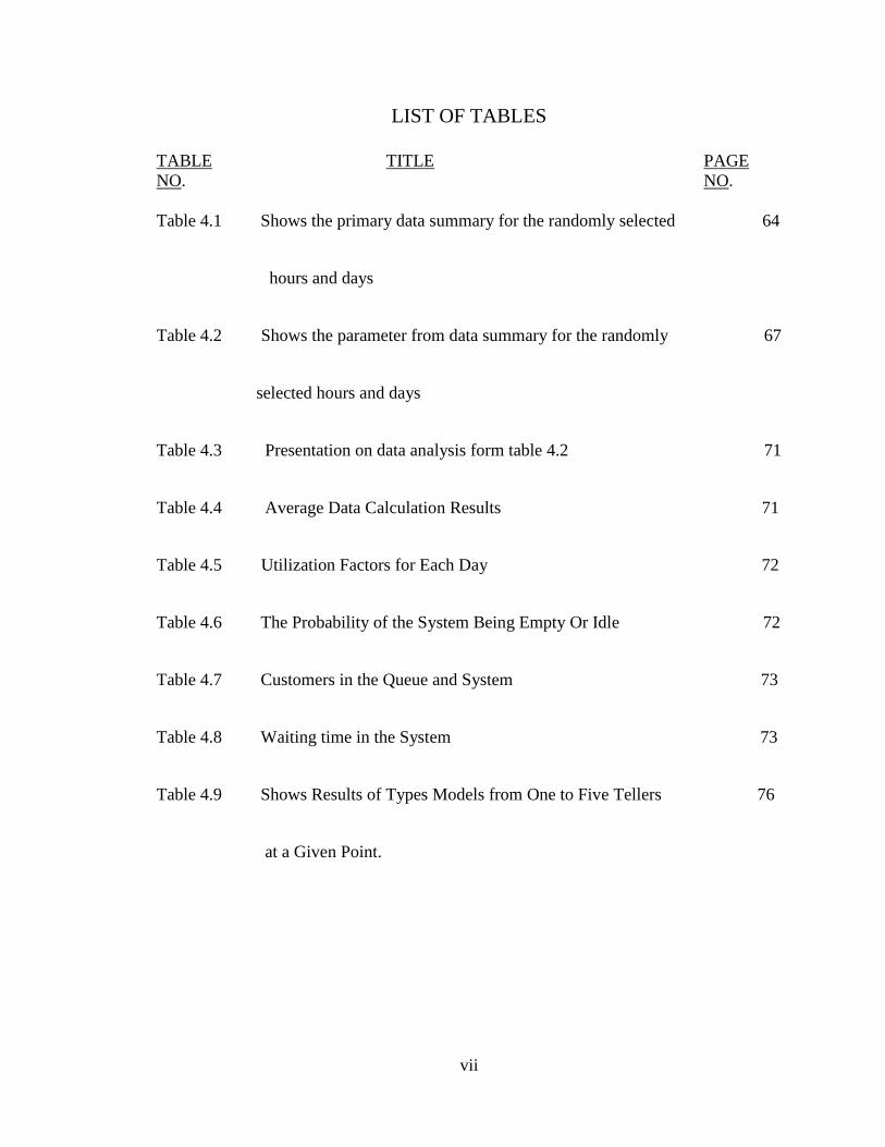
LIST OF TABLES

TABLE TITLE PAGE

NO. NO.

Table 4.1 Shows the primary data summary for the randomly selected 64

hours and days

Table 4.2 Shows the parameter from data summary for the randomly 67

selected hours and days

Table 4.3 Presentation on data analysis form table 4.2 71

Table 4.4 Average Data Calculation Results 71

Table 4.5 Utilization Factors for Each Day 72

Table 4.6 The Probability of the System Being Empty Or Idle 72

Table 4.7 Customers in the Queue and System 73

Table 4.8 Waiting time in the System 73

Table 4.9 Shows Results of Types Models from One to Five Tellers 76

at a Given Point.

viii

LIST OF FIGURES

FIGURE TITLE PAGE

NO. NO.

Figure 3.1 A Queuing System in the Banks. 32

Figure 3.2 Single Queue Single Server Diagram 35

Figure 3.3 Single Queue Multiple Servers Diagram 36

Figure 3.4 Multiple Queues Multiple Servers 37

Figure 3.5 Inter – arrivals and time at which the customer arrives 41

Figure 3.6 State Transitional rate diagrams for a single server 50

Figure 3.7 State Transitional Rate diagram for a multiple 56

Figure 4.1 A Graph Show the Arrival of Customers 66

ix

Dedication

This study is dedicated to Almighty God, Bannerman‘s family and my wife Enyonam

x

ACKNOWLEDGEMENTS

First and foremost, I thank God the Almighty for given me this opportunity and carrying

me through this thesis successfully. This thesis could not have been completed without

the support and encouragement from several people.

I am deeply indebted to my supervisor, Mr. Kwaku Dakwah, for his excellent direction,

invaluable feedback, his constructive suggestions, detailed corrections, support and

encouragement played enormous role resulted in this successful project.

I would like to extend my gratitude to all the academic and administrative staff of the

department of mathematics of KNUST.

I also own thanks and appreciate to the entire Bannerman‘s family for their

encouragement and support.

I thank the Managers of Ghana Commercial Bank, Harper Road, Kumasi for allowing the

collection of data for the study. Finally, this effort would not be possible without my wife

and brothers; their efforts and sacrifices have been of great helped towards the

completion of this thesis.

1

CHAPTER ONE

1.0 INTRODUCTION

This part consists of the background study of queuing, statement of problem, objective,

methodology, justification and organization of thesis.

1.1 BACKGROUND OF THE STUDY

In other to achieve serenity and discipline at service centers, queues are employed to

achieve these purposes. The act of queuing is associated with waiting, which is an

inevitable part of modern life. These actions range from waiting to be served at grocery

stores, banks and post offices to having to wait for an operator on a telephone call.

Furthermore, we often wait for a bus on our way to the work place, traffic lights to turn

green and lift at our office premises.

Non-familiar examples include broken down machines waiting for repairs, workmen

waiting for tools and goods in production shops waiting to be lifted by cranes. Even

situations of inventory may also be regarded as queues, in the sense that listed goods are

usually stored to await consumption.

All the above examples have one common feature i.e. customers arrive at service centers

and wait to be served. The arrival of customers is not necessarily regular and so the time

taken for service is not uniform. Queues build up during hours of demand and disappear

during the lull period.

Service rendered to customers almost always demand that they form queues. It is a

normal phenomenon for people to spend a great deal of time in queues or in waiting lines.

2

Queues run through all walks of life; be it academic, social and religious For example

queues are formed in banking halls, boarding of a bus to school, work or the hospital.

Activities in households are not to be left out i.e. queues are formed when it‘s time for

bathing and visiting the toilet. The trail is really endless and most often the experience

can be frustrating and costly.

Queues are present in a lot of service areas, from supermarkets, bus stops, taxi ranks, post

offices to video cinemas. Queues are associated with order and chaos usually erupts

whenever people try to jump queues. The experiences people go through in queuing at

service centres leaves much to be desired. These experiences sometimes culminate into

insults and in extreme cases fighting.

In general, there are two main types of queues, namely: physical queues and virtual

queues. Physical queues are organized queue areas commonly found at amusement parks

in which the rides have a fixed number of guests that can be served at any given time.

There has to be some control over additional guests who are waiting, leading to the

development of formalized queue areas. The areas in which people wait to board rides are

organized by barriers, and may be given shelter from roofs over their heads, inside a

climate-controlled building or with fans and misting devices. In some amusement parks,

queue areas are elaborately decorated, with various holding areas fostering anticipation,

thus, potentially shortening the perceived wait for some people in the queue. This

provides an interesting distraction to customers as they wait for their turn. There is a

perception that once customers are intrigued by the huge artifacts and designs, they serve

as a threshold of attraction as they wait. A prime example is the Walt Disney World in

USA.

3

Queues are generally found at transportation terminals where security screenings are

conducted. Sometimes there are separate queues for getting to service points. Large stores

and supermarkets usually have dozens of separate queues, but this can cause frustration

as different waiting lines tend to be handled at different speeds causing some people to be

served quickly, while others may wait for longer periods of time. Often times when two

people are in different queues immediately one realizes that the other queue moves faster,

the person quickly joins the other. A better arrangement, is for everyone one to wait in a

single queue and leave each time a service point opens up. This is commonly found in

several banking halls.

Physical queuing is sometimes replaced by virtual queuing. In a waiting room there may

be a system installed whereby a customer requests for his place in a queue or reports to a

desk and signs in, or takes a ticket with a number from an automated machine. These

queues are typically found in doctors' offices, hospitals, town halls, social security

offices, labour exchanges, department of motor vehicles, banks and post offices.

Currently in Ghana, tickets are now taken to form a virtual queue in several banking

halls. Some restaurants have also employed virtual queuing techniques with the

availability of application-specific pagers. This alerts customers in waiting to be seated.

Another option is to assign customers, a confirmed return time to serve as a reservation

issued on arrival.

It is evident in our everyday activities that there is a high probability for one to queue

before a service is rendered. Queues per say, are not a problem but if not managed well,

become a nuisance. The task, as a statistician, is to use existing theory of queuing systems

and statistical computing to see how best queues may be reduced or eliminated. It would

4

be of interest if mathematical models could be developed for the average queuing system

quantities, for example, waiting times, and using models to forecast by simulation any

situation in a particular system so as to ensure efficiency at service facilities. This will

cause great reduction or elimination in queues at automated service facilities. In the next

section, the objectives of the research are discussed.

In commercial or industrial sectors, it may not be economical to have waiting lines but

not feasible to totally avoid queues. An executive dealing with this system is to find the

optimal facilities provided. This is prudent because, banking is a commercial institution

and queues cannot be excluded from its operations.

A bank is generally understood as an institution which provides fundamental banking

services such as accepting deposits, cash management services for customers, reporting

transactions of their accounts and provision of loans. There are also nonbanking

institutions that provide certain banking services without meeting the legal definition of a

bank. Banks are a subset of the financial services industry. The banking system in Ghana

should not only be hassle free but be able to meet the new challenges posed by

technology other external and internal factors.

The history of banks in Ghana dates back to 1886 and 1917 when the first two banks

were established. These are the Bank of British West Africa, now Standard Chartered

Bank and Dominion, Colonial and Overseas now Barclays Banks of Ghana which were

established in 1886 and 1917 respectively as stated by Ankaah (1995). He also stated that

5

on the eve of independence, the banking industry had only one indigenous bank, called

Bank of Gold Coast now called Ghana Commercial Bank, established in 1953.

Ghana Commercial Bank Limited was established as a result of the need to provide

financial services to the indigenes of the then Gold Coast. Consequently, an ordinance for

the establishment of a native bank called Bank of Gold Coast was passed in October

1952. The bank of Gold Coast started operation in 1953. After Ghana‘s independence in

1957, the Bank of Gold Coast was renamed Ghana Commercial Bank. It has been

reported that the bank has fulfilled its mandate and continues to achieve remarkable

productivity in its area of operations (GCB Annual Report, 2010). As at today, the

government ownership stand at 26.14% while institutional and individual holding add up

to 73.86% of which SSNIT is the majority shareholder (GCB Annual Report, 2010)

From the start of one branch in the 1950, GCB Ltd now has 157 branches, l05 ATMs and

15 agencies (GCB Diary, 2008). GCB is endowed with high quality human resource

which stands at 2185. This is remarkable when one consider that the bank started with

staff strength of 27 and as branches increased so did the staff. Currently there are

professionals of various disciplines who work in tandem to achieve the objectives of the

bank.

The bank has grown through this divesture era and has several branches across the

breadth of the country and almost operates in every district of the country. The bank is

now listed on the Ghana stock exchange market in 1996. The growth of the bank has

been synonymous with its customer base, performance, innovative product and services,

6

profitability and corporate social responsibility. GCB has taken advantage of enhance

information technology system and introduced internet banking, royal banking, mobile

banking, smart pay system and international remittance like money gram. GCB Ltd is the

widest networked bank in Ghana. All these have been done to increase profit and enhance

shareholders value. (GCB Limited Diary (2008) and GCB Limited Annual Report, 2010).

The necessity of a controlling or regulating agency or institution was naturally felt. So

after independence the Bank of Ghana (BOG) was established in 1957, so as to check and

control the banking institutions.

The competition in the banking sector is getting more intense, partly due to regulatory

imperatives of universal banking and also due to customers‘ awareness of their rights.

Bank customers have become increasingly demanding, as they require high quality, low

priced and immediate service delivery. They want additional improvement of value from

their chosen banks (Olaniyi, 2004). Service delivery in banks is personal, customers are

either served immediately or join a queue (waiting line) if the system is busy. A queue

occurs where facilities are limited and cannot satisfy demand made against them at a

particular period. However, most customers are not comfortable with waiting or queuing

(Olaniyi, 2004). The danger of keeping customers in a queue is that their waiting time

could become a cost to them. According to Elegalam (1978), customers are prepared not

to spend more cost of queuing. The time wasted on the queue would have been

judiciously utilized elsewhere (the opportunity cost of time spent in queuing).

There have been immense developments in Ghana‘s banking sector since the period of

financial sector reforms. A key development was the entry of private banks into the

7

market and the expansion of branches of existing banks. This was followed by

development of new technologies to deliver financial services, such as Automated Teller

Machines (ATMs), Electronic Funds, Transfer at Point of Sale (EFTPOS) and other

stored value cards. These cost-effective innovations and products have the purpose of

reducing the pressure on over-the-counter services to bank customers. According to Abor

(2004), arguably the most revolutionary electronic innovation in Ghana and the world

over has been the introduction of ATM‘s. Another technological innovation in Ghanaian

banking is the various electronic cards, which the banks have developed over the years.

Banks as financial intermediaries provide convenience and liquidity for their clients. The

technological wave across the globe, especially the use of information and

communication technologies (ICT) has affected the conduct of business generally as

stated by Marfo - Yiadom (2012).

These long queues can be analyzed as results of the following characteristics in queuing

systems. These characteristics are grouped into problems for the queuing processes. This

provides an adequate description of the queuing system i.e. arrival problems of

customers, behavioural problems, statistical problems and operational problems. The

objective analysis of queuing systems is to understand the behaviour of their underlying

processes so that informed and intelligent decisions can be made in their management.

These types of problems can be identified by the following processes:

Arrival process (or pattern) of customers to the service system is classified into two

categories, namely static and dynamic process. These two are further classified based on

the nature of arrival rate and the control that can be exercised on the arrival process.

8

In static arrival process, the control depends on the nature of arrival rate (random or

constant). Random arrivals are either at a constant rate or varying with time. Thus to

analyze the queuing system, it is necessary to attempt to describe the probability

distribution of arrivals.

From such distributions we obtain average time between successive arrivals, also called

inter-arrival time (time between two consecutive arrivals), and the average arrival rate

(i.e. number of customers arriving per unit of time at the service system). The dynamic

arrival process is controlled by both service facility and customers. The service facility

adjusts its capacity to match changes in the demand intensity, by varying the staffing

levels at different timings of service, varying service charges such as telephone call

charges at different hours of the day or week, or allowing entry with appointments.

Frequently in queuing problems, the number of arrivals per unit of time can be estimated

by a probability distribution known as the Poisson distribution, as it adequately supports

many real world situations

Behavioral problem involves the study of queuing system that is intended to understand

how it behaves under various conditions. The bulk of results in queuing theory are based

on research on behavioral problems. Mathematical models for the probability

relationships among the various elements of the underlying process are used in the

analysis. A collection or a sequence of random variables that are indexed by a parameter

such as time is known as a stochastic process e.g. a timely record of the number of people

who enter the bank. In the context of a queuing system the number of customers with

time as a parameter is known as a stochastic process. Let Q (t) be the number of

9

customers in a system at time t. This number is the difference between number of arrivals

and departures during (0, t). Let A (t) and D (t), respectively, be these numbers. A simple

relationship would then be Q(t)=A(t)−D(t). In order to manage the system efficiently one

has to understand how the process (t) behaves over time. Since the process Q(t) is

dependent on A(t) and D(t), both of which are also stochastic processes, their properties

and dependence characteristics between the two should also be understood. All these are

idealized models to varied degrees of realism. As done in many other branches of

science, they are studied analytically with the hope that the information obtained from

such study will be useful in the decision making process. In addition to the number of

customers in the system, known as the queue length, the time a new arrival has to wait till

its service begins, which we call the waiting time, and the length of time the server is

continuously busy, which we call the busy period, are major characteristics are of

interest. It should be noted that the queue length and the waiting time are stochastic

Processes and the busy period is a random variable. Distribution characteristics of the

stochastic processes and random variables are needed to understand their behavior. Since

time is a factor, the analysis has to make a distinction between the time dependent, also

known as transient, and the limiting, also known as the long term, behavior. Under

certain conditions a stochastic process may settle down to what is commonly called a

steady state or a state of equilibrium, in which its distribution properties are independent

of time.

Statistical problems include the analysis of empirical data in order to identify the correct

mathematical model, and validation methods to determine whether the proposed model is

appropriate. For an insight into the selection of the correct mathematical model, which

10

could be used to derive its properties, a statistical study is fundamental. In the course of

modeling we make several assumptions reading the basic elements of the model.

Naturally, there should be a mechanism by which these assumptions could be verified.

Starting with testing the goodness of fit for the arrival and service distributions, one

would need to estimate the parameters of the model and/or test hypotheses concerning the

parameters or behavior of the system. Other important questions where statistical

procedures play a part are in the determination of the inherent dependencies among

elements and dependence of the system on time.

Operational problems are inherent in the operation of queuing systems. Example of such

problem is statistical in nature. Others are related to the design, control, and the

measurement of effectiveness of the system.

All these innovations are adapted to reduce queues in banking halls but sometimes there

are interestingly good electronic innovations found in these places. Notwithstanding the

use of technologies, branches that are being opened day in day out still experiences great

queues in their various baking halls. The queuing system in banking halls need to be

analyzed well so as to prevent the increase in waste of time and idleness of customers.

1.2 STATEMENT OF THE PROBLEM

It is not desirable to have long queues due to time and money constraints; however

queues seem so alive in our day-to-day activities. In Ghana Commercial Bank, the

existent problem of long queues in the banking halls for hours causes loss of precious

time, limits productivity and makes patronage more tedious. In view of the vital role that

11

banks play in the economy of a country, a slight decline in performance may largely have

an adverse effect on the country‘s economy. Queuing in banking halls has great negative

consequences apart from leading to chaos and loss of man hours per day. Performing

these financial activities could be time consuming and tedious because of the inherent

traditional methods of banking. During the analysis of an informal survey carried out on

some customers at GCB Harper Road Branch, it was revealed that majority of customers

complained about the amount of time spent in queues before they are attended to by a

teller. Owing to these complains it has become prudent to use a mathematical model to

check the queuing system at Ghana Commercial Bank Harper Road, Kumasi.

1.3 OBJECTIVES OF THE STUDY

The ultimate objective of this study is to analyze queuing systems at Ghana Commercial

Bank in other to understand the behaviour of their underlying processes for informed

decisions to be taken by management.

Subsequently, an attempt is made to achieve the following specific objectives:

• To use a mathematical model for the determination of waiting time in a queue.

• How waiting time will be affected, if there are alterations in the facilities

available.

12

1.4 METHODOLOGY

In a business, time is an essential commodity and need not to be wasted, for this reason

the problem of wasting much time whiles in a queue will be modelled. Analysis on

waiting time in banking halls will be done using the developed model. This will be based

on a simple markovian model for data collection and analysis.

The source of primary data will be collected at Ghana Commercial Bank, Harper Road,

(Kumasi) for the analysis. It will be collected during two different sessions that is peak

days and non-peak days. In addition, other sources of information for this study are the

internet, KNUST library, past research works, articles and journals for relevant literature.

1.5 JUSTIFICATION

Queuing systems primarily involve the provision of services. These systems involve the

arrival and departure of customers at service centres in search of efficient services.

Queuing system extend beyond waiting lines in banking halls and the usual phenomenon

of delay caused by busy servers. The systematic study of queuing system may be useful

in contributing towards other areas in the society such as:

Analysis of reducing waiting time in banking halls and other areas

Recommending to institutions after the research.

Serves as statistical science that has too much to offer in many fields of human

activity

13

Reductions of queues in banking halls help attract more customers to join their

services.

1.6 ORGANIZATION OF THE STUDY

The study is organized into five chapters. Chapter one talks about the introduction of the

study.

This includes the background of the study, problem statement, significance and

objectives of the study, research questions, methodology, limitations and organization of

the study.

In chapter two, pertinent literature in the area on queuing systems or models shall be

reviewed. The profile of GCB and the detailed methodology used in this study shall be

presented in chapter three. Chapter four is solely for data collection and analysis. The

final chapter which is chapter five concludes the study with the summary of major

findings, conclusion and recommendations.

14

CHAPTER TWO

LITERATURE REVIEW

2.0 INTRODUCTION

This chapter gives adequate and relevant literature on queuing systems in the banking

industry, modelling of the queuing theory, queuing theory, effects of queuing, queuing

managements, methods and illustrative examples of queuing systems, empirical and

theoretical review of queuing systems in the banking industry and the importance and

disadvantages of queuing systems are presented.

2.1 THE HISTORY OF QUEUING

Queuing has existed through centuries and time in memorial, but still leaves some of its

technique and history more never-ending than the creatures of geology. It has been one of

the primitive ways of optimizing some real life problems up to date. The major reason for

using a queue in all areas is to provide fair service to customers. In addition, experimental

psychology studies show how fair scheduling in queuing systems is indeed highly

important to humans.

According the web (askville) the concept of lining up dates to the Bible, at least "Queue"

from Latin to French to English. 1837 is conventional date. For the invention of the

concept of the queue, here‘s the first historical reference. According to Bible in Genesis

7:8, it reads "Of clean beasts, and of beasts that are not clean, and of fowls, and of

everything that creepeth upon the earth, There went in two and two unto Noah into the

ark, the male and the female, as God had commanded Noah." i.e. they lined up two by

15

two, a very orderly British sort of thing to do. You would too, if God was calling the

shots. Of course, they didn‘t call it a queue, but from then on the question is what to call a

line of people. The earliest written use I could find of queue meaning a line was the

Bayou Queue de Tortue, a part of Louisiana with that name purchased in 1801 by an

American. At that time, the meaning was "line of turtles", so we therefore have a French

word in use with the "line" meaning by Americans back at least to 1801 (yes, I‘m

stretching, but isn‘t that part of the fun - maybe to discover something new?).

The conventional story on the origin is that it is French (out of Latin coda), from the

French cue, a word originally meaning "tail", but evolving over time by the 1700s at least

in French to also Bhat (2008) states that the study of the history of queuing theory dates

back to over a century, the first paper on the subject seems to be Johannsen‘s paper

"Waiting Times and Number of Calls" (an article published in 1907 and reprinted in the

Post Office Electrical Engineers Journal, London, October, 1910). From the point of view

of an exact treatment, the method used in the paper was not mathematically exact and

therefore, the paper that has historical importance is Erlang‘s (1909), "The Theory of

Probabilities and Telephone Conversations", which contains some of the most important

techniques and concepts in queuing theory; for instance the notion of statistical

equilibrium and the method of formulating the balance of state equations (later called

Chapman-Kolmogorov equations)

16

2.2 QUEUES

Several definitions have been given to queues by different scholars. According to Black

(2006), a queue is a collection of items in which only the earliest added item may be

accessed. Basic operations are add (to the tail) or enqueue and delete (from the head) or

dequeue. Delete returns the item removed. This is also known as "first-in, first-out" or

FIFO‖ This type of queue is a buffer abstract data structure. Wikipedia also gives the

meaning of a queue as a line of people or vehicles waiting for something.

With the data structure meaning of queue, the most well-known operation of the queue is

the First-In-First-Out (FIFO) queue process. In a FIFO queue, the first element in the

queue will be the first one out; this is equivalent to the requirement that whenever an

element is added, all elements that were added before have to be removed before the new

element can be invoked. Unless otherwise specified, the remainder of the article will refer

to FIFO queues in Wikipedia (2012).

Hongna and Zhenwei (2010) stated that queuing in a bank is a common phenomenon

and also a knotty problem. Their paper first processes collected line data of banks, gets

distribution and parameters on customers arriving and the service time interval, then take

a simulation by witness and put forward optimization measures. The assessments of two

queuing strategies, taking the average length of staying and the average time of queuing

in system as indexes, can play a role in the choice of the queuing way of multi-desks

servers, at the same time, show it is one of effective measures, to improve efficiency of

bank server system, that the calling number machine changed from multi queues and

multi desks to single queue and multi desks system.

17

According to Zhou and Soman (2003) queues are a ubiquitous phenomenon. The research

investigates consumers‘ affective experiences in a queue and their decisions to leave the

queue after having spent some time in it (reneging). In particular, they found in their first

two studies that, as the number of people behind increases, the consumer is in a relatively

more positive affective state and the likelihood of reneging is lower. While a number of

explanations may account for this effect, they focused on the role of social comparisons.

In particular, they expected consumers in a queue to make downward comparisons with

the less fortunate others behind them. And also proposed that three types of factors

influence the degree of social comparisons made and thus moderate the effect of the

number behind: (a) queue factors that influence the ease with which social comparisons

can be made, (b) individual factors that determine the personal tendency to make social

comparisons, and (c) situational factors that influence the degree of social comparisons

through the generation of counterfactuals. Across three studies, they found support for

each moderating effect and concluded with a discussion on theoretical implications and

limitations, and we propose avenues for future research.

2.3 QUEUING THEORY

Wikipedia defines queuing theory as, ―the mathematical study of waiting lines (or

queues)‖. These theories allows for the mathematical analysis of several related

processes, including entering the queue, waiting in the queue and exiting the queue. It

continues to state that, ―The theory permits the derivation and calculation of several

performance measures including the average waiting time in the queue or the system, the

expected number waiting or receiving service and the probability of encountering the

18

system in certain states, such as empty, full, having an available server or having to wait

a certain time to be served‖. Mandia (2006) also defines queuing theory as being

essentially the study of a queue through the use of mathematical modeling to evaluate the

efficiency of queues. It is the basis to finding the optimal solution to queue management.

Consistent with Wikipedia contributors three types of queues are identified that are

widely used involving queue theory. They include First In First Out, Last In First Out and

Processor Sharing. In First In First Out, the item in the queue that has been in the queue

the longest would be the first to be removed from the queue. In First In Last Out, the item

in the queue for the shortest amount of time would be the first to exit the queue. The

Processor Sharing discipline serves all the items in the queue equally.

Queuing theory provides long-run steady state performance measures and is thus a good

fit for making long-term strategic decisions. Crowley et al (1995) present a queuing

analysis performed during the initial design of a production facility for electromechanical

devices. The procedure, described as flow ratio analysis, is based on Jackson queuing

networks and provides an early estimate for labor and resource requirements before the

construction of a more detailed simulation model.

In addition queuing theory as said by Vasumathi and Dhanavanthan (2010)

has been applied to a variety of business situations such as banks, transportation areas,

hospitals and all situations are related to customer involvement.

Generally, the customer expects a certain level of service, whereas the firm provides

service facility and tries to keep the costs minimum while proving the

19

required service. This is widely used in manufacturing units to help in reducing the

overhead charges and the overall cost of manufacture. Also used to know is the unit

arrive, at regular or irregular interval of time at a given point called the service.

2.4 QUEUING MODELS

As said by Prikryl and Kocijan (2012), Mathematical modeling is an inevitable part of

system analysis and design in science and engineering. When a parametric mathematical

description is used, the issue of the parameter estimation accuracy arises. Models with

uncertain parameter values can be evaluated using various methods and computer

simulation is among the most popular in the engineering community. Nevertheless, an

exhaustive numerical analysis of models with numerous uncertain parameters requires a

substantial computational effort. The purpose of the paper is to show how the

computation can be accelerated using a parallel configuration of graphics processing

units (GPU). The assessment of the computational speedup is illustrated with a case

study. The case study is a simulation of Highway Capacity Manual 2000 Queue Model

with selected uncertain parameters. The computational results show that the parallel

computation solution is efficient for a larger amount of samples when the initial and

communication overhead of parallel computation becomes a sufficiently small part of the

whole process

In a study by Brown (2012), queuing models can help managers to understand and

control the effects of rework, but often this tool is overlooked in part because of concerns

over accuracy in complex environments and/or the need for limiting assumptions. One of

20

the aims of his work is to increase understanding of system variables on the accuracy of

simple queuing models. A queuing model is proposed that combines G/G/1 modeling

techniques for rework with effective processing time techniques for machine availability

and the accuracy of this model is tested under varying levels of rework, external arrival

variability, and machine availability. Results show that the model performs best under

exponential arrival patterns and can perform well even under high rework conditions.

Generalizations are made with regards to the use of this tool for allocation of jobs to

specific workers and/or machines based on known rework rates with the ultimate aim of

queue time minimization

Khalaf (2012) in his work ascertained that during the next two decades several

mathematicians became interested in these problems and developed general models

which could be used in more complex situations. The first use of the term "queuing

system" occurred in 1951 in the Journal of the Royal Statistical Society, when D.C.

Kendall published his article "Some Problems in the Theory of Queues". Of course, there

were a huge number of articles on the subject much earlier (some used the word "queue"

but not the word "queuing").

Nosek and Wilson (2001) stated that queuing theory utilizes mathematical models and

performance measures to assess and hopefully improve the flow of customers through a

queuing system. Queuing theory has many applications and has been used extensively by

the service industries. Queuing theory has been used in the past to assess such things as

staff schedules, working environment, productivity, customer waiting time, and customer

waiting environment.

21

A queuing system or waiting line phenomenon consists essentially of six major

components: the populations, the arrival, queues itself, queue discipline, service

mechanism and the departure or exit.

Udayabhanu et al (2010) established that congestion in queuing systems has serious

consequences, so that it is never optimal to operate at 100% utilization levels. We

develop an expression for the optimal utilization level for an M/D/1 queue, and

demonstrate its similarity to the EOQ model of the inventory literature. The model can be

used to achieve an optimal mean arrival rate, or to appropriately adjust the available

capacity so that the desired utilization level is attained.

Gurumurthi and Benjaafar consider queuing systems with multiple classes of customers

and heterogeneous servers where customers have the flexibility of being processed by

more than one server and servers possess the capability of processing more than one

customer class. They provided a unified framework for the modeling and analysis of

these systems under arbitrary customer and server flexibility and for a rich set of control

policies that includes customer/server-specific priority schemes for server and customer

selection. They used their models to generate several insights into the effect of system

configuration and control policies. In particular, the model examines the relationship

between flexibility, control policies and throughput under varying assumptions for

system parameters.

22

Rouba and Ward (2009) in their used heavy – traffic limits and computer simulation to

study the performance of alternative real – time delay estimators in the overloaded GI/GI/

s+ GI multi server queuing model, allowing customer abandonment. These delay

estimates may be used to make delay announcements in call centers and related service

systems. They characterized the performance of the system by the expected mean squared

error in steady state. In addition they established approximations for performance

measures with a non-exponential abandonment-time distribution to obtain new delay

estimators that effectively cope with non-exponential abandonment-time distributions

2.5 EFFECTS OF QUEUING

Bank et al (2001),they concluded that delays and queuing problems are most common

features not only in our daily-life situations such as at a bank or postal office, at a

ticketing office, in public transportation or in a traffic jam but also in more technical

environments, such as in manufacturing, computer networking and telecommunications.

They play an essential role for business process re-engineering purposes in administrative

tasks. ―Queuing models provide the analyst with a powerful tool for designing and

evaluating the performance of queuing systems.‖

According to Sokefun (2011), Customer satisfaction is derived largely from the quality

and reliability of products and services. However, almost every Nigerian bank encounters

similar problems in meeting customer‘s expectation of services and customer satisfaction.

For example, the issue of money transfer in banks is one major problem that customers of

certain banks have been made to experience. In most cases the customer hardly receives

23

the payment of the money transferred into account immediately. The long queues and

huge crowds in the banking halls can be highly devastating and discouraging most times,

especially when the weekend is near. Most times, this long queues are as a result of the

breakdown of the computers used by these cashiers, sometimes it occurs as a result of the

cashiers, pushing duty to one another as to who is to attend to the customers or not.

On the word of Zeithaml (2000), the major problems in measuring the relationship are;

the time lags between measuring customer satisfaction and profit improvement, the

number of other variables influencing performance such as pricing, convenience,

transaction methods and system, customer care and so on should be included in the

relationship because they explain the causality between satisfaction and result.

However, the problems faced by banks in delivering effective services to customers

include; insufficient legal system, high provisions for non-performing loans, high lending

rates, poor management, political instability, high pricing of financial services, higher

risks and low profitability. These have in turn affected their quality of service offered.

Most times, these negative effects limit the number of prospective customers who

patronize banking services. This is because a customer who has once been disappointed

by a bank‘s services decides to tell others not to use that same service.

According to Larson, (1987), once banks have cut waiting lines, such acts cease to be

customer services. Furthermore, waiting time from the viewpoint of service industry has

effect of the number of customers that are willing to patronize a particular bank. In other

to build a cordial and lasting relationship with the customers, the bank must supply the

24

best service to maximize customer satisfaction and increase service efficiency by

providing prompt or timely service. Waiting for service is typically a negative consumer

experience and cause unhappiness, frustration, and anxiety by consumer. Due this there

must be ways in which queues must be reduced so as to make consumers patronized

banking services

Even at the hospital, people queue to be talking care of in which the effect of queuing

during hospital visits in relation to the time spent for patients to access treatment in

hospitals is increasingly becoming a major source of concern to a modern society that is

currently exposed to great strides in technological advancement and speed according to

Stakutis and Boyle, (2009)

Customer service is the provision of service to customers before, during and after a

purchase. Along with Turban et al. (2002), ―customer service is a series of activities

designed to enhance the level of customer satisfaction- that is, the feeling that a product

or service has met the customer expectation.‖ Customer service may be provided by a

person (e.g., sales and service representative), or by automated means called self-service.

Customer service is normally an integral part of a company‘s customer value proposition.

From the point of view of an overall sales process engineering effort, customer service

plays an important role in an organization‘s ability to generate income and revenue. From

that perspective, customer service should be included as part of an overall approach to

systematic improvement. A customer service experience can change the entire perception

a customer has of the organization.

25

According to Osuagwu (2002), Customer service is concerned establishing, maintaining

and enhancing relationships between and/or among relevant business parties in order to

achieve the objective of the relevant parties. Such parties are usually, but not necessarily

always, long-term oriented. He explains customer service as a situation where every

customer is considered as an individual, activities of the organization or institution

directed towards existing customers based on interaction and dialogue with relevant

parties achieving set organizational goals and objective.

In relation to Lucas (2005), customer service is defined as the ability of knowledgeable,

capable and enthusiastic employees to deliver products and services to their internal and

external customers in a manner that satisfies identified and unidentified needs and

ultimately result in positive word-of-mouth publicity and return business

2.6 QUEUING MANAGEMENT

The first step in active queue management is determining the offered load. In particular,

we must detect high-bandwidth flows and estimate their sending rates. In their work, we

apply the sample-and-hold technique proposed by Estan and Varghese (2002)

Gosha (2007) talks of Queue Management as being a problem for many years in many

domains including the Financial Services, Health Care, Public and Retail Sectors. In this

age of technology it is not only important to organize the existing queue, but to gather

statistics about the queue in order to identify trends that could be anticipated. For many

barbershops, these needs are not addressed in a sophisticated manner. The study suggests

that a Queue Management System such as Queue Administration will improve the

satisfaction of a shop‘s customers as well as their barbers. The tool used in the study,

26

Queue Administration, is a database driven, online application to manage the different

waiting list of a barbershop.

AL-Jumaily and AL-Jobori (2011) cited that their paper focuses on the banks lines

system, the different queuing algorithms that are used in banks to serve the customers,

and the average waiting time. The aim of their paper was to build automatic queuing

system for organizing the banks queuing system that can analyses the queue status and

take decision which customer to serve. The new queuing architecture model can switch

between different scheduling algorithms according to the testing results and the factor of

the average waiting time. The main innovation of their work concerns the modeling of

the average waiting time is taken into processing, in addition with the process of

switching to the scheduling algorithm that gives the best average waiting time.

In relation to Jong-hwan et al (2011) two major goals of queue management are flow

fairness and queue-length stability However, most prior works dealt with these goals

independently. In the paper, they shown that both goals can be effectively achieved at the

same time and proposed a novel scheme that realizes flow fairness and queue-length

stability. In the proposed scheme, high-bandwidth flows are identified via a multilevel

caching technique. Then, they calculated the base drop probability for resolving

congestion with a stable queue, and apply it to individual flows differently depending on

their sending rates. Via extensive simulations, they shown that the proposed scheme

effectively realizes flow fairness between unresponsive and TCP flows, and among

heterogeneous TCP flows, while maintaining a stable queue.

27

Sohraby et al (2004), stated in their work that Active queue management (AQM) is an

effective method to enhance congestion control, and to achieve tradeoff between link

utilization and delay. The de facto standard, random early detection (RED), and most of

its variants use queue length as a congestion indicator to trigger packet dropping. The

proportional-integral (PI), use both queue length and traffic input rate as congestion

indicators; effective stability model and practical design rules built on the TCP control

model and abstracted AQM model reveal that such schemes enhance the stability of a

system. They proposed an AQM scheme with fast response time, yet good robustness.

The scheme, called loss ratio based RED (LRED), measures the latest packet loss ratio,

and uses it as a complement to queue length in order to dynamically adjust packet drop

probability. Employing the closed-form relationship between packet loss ratio and the

number of TCP flows, this scheme is responsive even if the number of TCP flows varies

significantly. They also provide the design rules for this scheme based on the well-known

TCP control model. This scheme's performance is examined under various network

configurations, and compared to existing AQM schemes, including PI, random

exponentially marking (REM), and adaptive virtual queue (AVQ). Our simulation results

show that, with comparable complexity', this scheme has short response time, better

robustness, and more desirable tradeoff than PI, REM, and AQV, especially under highly

dynamic network and heavy traffic load.

2.7 METHODS OF SOLUTION AND ILLUSTRATIVE WORKS

The present study concerns single – server queues where the inter arrival times and the

service times depend on a common discrete time Markov Chain; i.e. the so – called semi

– Markov queues. As such, the model under consideration is a generalization of the

28

MAP/G/1 queue, by also allowing dependencies between successive service times and

between interval times and services times.

In order to service the customers at faster rates, there must be good customer advisors,

faster computers and better networks provided the computers are networked to avoid

queuing or jamming networks. The need to analyze service mechanism in the rapidly

growing computer and communication industry is the primary reason for strengthening of

queuing theory after the 1960‘s. Research on queuing networks and books as Coffman

and Deming, 1973; Kleinrock, 1976 laid the foundation for a vigorous growth of the

subject. In tracking this growth, one may cite the following survey type articles from the

journal Queuing Systems: Coffman and Hoffri, 1986, describing importance of computer

devices and the queuing models used in analyzing their performance.

Filipowicz and Kwiecien (2008) stated in their article by describing queuing systems and

queuing networks as successfully used for performance analysis of different systems such

as computer, communications, banking halls, transportation networks and manufacturing.

It incorporates classical Markovian systems with exponential service times and a Poisson

arrival process, and queuing systems with individual service. Oscillating queuing systems

and queuing systems with Cox and Weibull service time distribution is an example of

non-Markovian systems.

Usmanov and Jarsky (2009) stated in their work that queues theory examines systems

with operating channels, where the process of queues formation takes place and

subsequent servicing of the customers by servicing centers. The main objective of the

29

queues theory is to determine the laws under which the system works, and further to

create the most accurate mathematical model that takes into account various stochastic

influences on the process. The entire construction process can be examined from the

point of view of a customer who is waiting in the queue and is interested primarily in the

waiting time, as well as from the point of view of servicing centers. A waiting element

decides if you join the queue, or to go to another system entirely. In terms of servicing

centers, the priority is to determine the occupancy of the channel and the probability of

failure, including the time of repair. A servicing center should also reliably identify the

time per customer service, taking into account the current construction task

According to Jean-Marie and Hyon (2009), they consider a single server queue in discrete

time, in which customers must be served before some limit sojourn time of geometrical

distribution. A customer who is not served before this limit leaves the system: it is

impatient. The fact of serving customers and the fact of losing them due to impatience

induce costs. The purpose is to decide when to serve the customers so as to minimize

costs. They use a Markov Decision Process with infinite horizon and discounted cost.

They established the structural properties of the stochastic dynamic programming

operator and deduced that the optimal policy is of threshold type. In addition, they

compared and analyzed two threshold policies, which were able to compute explicitly the

optimal value of this threshold according to their parameters of the problem.

Nafees (2007), in his paper stated that analysis of Queuing systems for the empirical data

of supermarket checkout service unit as an example. One of the expected gains from

studying queuing systems is to review the efficiency of the models in terms of utilization

30

and waiting length, hence increasing the number of queues so customers will not have to

wait longer when servers are too busy. In other words, trying to estimate the waiting time

and length of queue(s), is the aim of his research paper. Use queuing simulation to obtain

a sample performance result and we are more interested in obtaining estimated solutions

for multiple queuing models.

According to Majakwara (2009), his thesis dealt mainly with the general M / GI / k

model with abandonment. The arrival process conforms to a Poisson process; service

durations are independent and identically distributed with a general distribution, there are

k servers, and independent and identically distributed customer abandoning times with a

general distribution. The thesis will endeavour to analyze call centers using M / GI / k

model with abandonment and the data to be used will be simulated using EZSIM –

software.

Mickevicius and Valakevicius (2006) stated that the purpose of their paper is to suggest a

method and software for evaluating queuing approximations. A numerical queuing model

with priorities is used to explore the behaviour of exponential phase-type approximation

of service-time distribution. The performance of queuing systems described in the event

language is used for generating the set of states and transition matrix between them. Two

examples of numerical models are presented – a queuing system model with priorities

and a queuing system model with quality control

31

Tabari et al (2012) in their work concluded that multi-server queuing analysis can be used

to estimate the average waiting time, queue lengths, number of servers and service rates.

These queuing models approximate the performance of queuing systems with multiple

queues. In their paper, they use the queuing theory to recognize the optimal number of

required human resources in an educational institution carried out in Iran. The queue

analysis is performed for different numbers of staff members. Finally, the result of their

study shows that the staff members in this department should be reduced.

32

CHAPTER THREE

3.0 METHODOLOGY

3.1.0 GENERAL OVERVIEW OF QUEUING SYSTEM

The queuing system consists essentially of three major components: (1) the source

population and the way customers arrive at the system, (2) the servicing system, and (3)

the condition of the customers exiting the system (back to source population or not?). The

system consist of more servers, an arrival pattern of customer, service pattern, queue

discipline, the order in which services is provided and customer behavior. There are

several everyday examples that can be described as queuing systems, such as bank-teller

service, computer systems, manufacturing systems, maintenance systems, communication

systems and so on. The following sections discuss each of these areas

Served

Customers

Leaving

Queuing

Capacity

Discouraged customers

leaving

Figure 3.1 A Queuing System in the Banks.

Service

Mechanism

s

Queue Customer

Serving

Customers

Calling

Population

Arrival

Process

Queuing discipline

33

3.1.1 ARRIVAL PROCESS

Arrivals may originate from one or several sources referred to as the calling population.

The calling population can be limited or 'unlimited'. An example of a limited calling

population may be that of a fixed number of machines that fail randomly. The arrival

process consists of describing how customers arrive to the system.

If is the inter-arrival time between the arrivals of customers,

we shall denote the mean (or expected) inter-arrival time by

and 𝜆 is the arrival frequency.

3.1.2 SERVICE MECHANISM

The service mechanism of a queuing system is specified by the number of servers

(denoted by s), each server having its own queue or a common queue and the probability

distribution of customer's service time.

Let be the service time of the ith customer, we shall denote the mean service time of a

customer by E(S) and the service rate of a server.

3.1.3 QUEUE DISCIPLINE

Discipline of a queuing system means the rule that a server uses to choose the next

customer from the queue (if any) when the server completes the service of the current

customer. Commonly used queue disciplines are:

FIFO - Customers are served on a first-in first-out basis.

34

LIFO - Customers are served in a last-in first-out manner.

Priority - Customers are served in order of their importance on the basis of their service

requirements.

In the system customers behaves in the following ways

Balking: some customers show reluctance for waiting in the queue. They do not

join the queue at their correct position and attempt to jump the queue and reach

the service centre by passing others ahead of them

Reneging: some customers after waiting sometime in the queue leave the queue

without getting the service due to impatience.

Collusion: some of the customers join together and only one of them will be in

the queue, instead of all staying in the queue. However, when their turn comes

for service, all the customers who were in collusion demand for service.

Jockeying: in case there is more than one queue for similar type of service, some

customers keep on shifting from one queue to another queue to improve their

position and to get immediate service.

3.2.0 TYPES OF QUEUES AND THEIR STRUCTURES IN THE BANKS

There are different types of queues and some examples are simple queue (first come first

out), circular queue, priority queue and de – queue (double ended queue). System in the

banking hall which is most frequently used is the simple queue which involves multiple

queues and single queues. In addition to that the servers (tellers) also determine how long

someone can be at the banking hall.

35

3.2.1 SINGLE QUEUE AND SINGLE SERVER (TELLER)

In this type of queuing system if server becomes idle a customer moves to the teller to be

served immediately, if not an arriving customer joins a queue and when the server has

completed serving a customer, the customer leaves the system. If there are customers

waiting in a queue, one is immediately dispatched to the server for transactions.

This type of queue is practices at the areas where customers follow that queue to make

enquires, check balance and open new accounts.

3.2.2 SINGLE QUEUE AND MULTIPLE SERVERS (TELLERS)

This type of system shows a multiple servers with all sharing a common queue. This is

the type of queue used in Ghana Commercial Bank, Harper Road Branch as shown in the

Arrival Point

Queue

Departure

Server

Figure 3.2 Single Queue Single Server Diagram

Single Queue Single Server

36

figure 3.3. If a customer arrives and at least a teller is available, then the customer will be

served immediately. It is assumed that all the servers are identical and thus if more than

one server is available, it makes no difference which server is chosen for the customer to

be served. If all the servers are occupied, a queue begins to form. As soon as one server

becomes free, a customer is asked to come so that the customer to be served.

3.2.3 MULTIPLE QUEUE AND MULTIPLE SERVERS (TELLERS)

This can also be called Single Stag Queue in Parallel as described in Figure 3.4. It is

similar to that of Single Queue – Server Queue, only that there are many servers (tellers)

Arrival Point

Queue

Departure

Departure

Single Queue Multiple Servers

Figure 3.3 Single Queue Multiple Servers Diagram

Servers

37

performing the same task with each having a queue to be served. This type of queue is

practiced in other branches of Ghana Commercial Bank as well as other banks.

3.3 MEASURES OF PERFORMANCE FOR QUEUING SYSTEMS:

Relevant performance measures in the analysis of queuing models are:

The distribution of the waiting time and the sojourn time of a customer. The

sojourn time is the waiting time plus the service time.

The distribution of the number of customers in the system (including or excluding

the one or those in service).

Multiple Queues Multiple Servers

Departure

Departure

Arrival Point

Queues

Figure 3.4 Multiple Queues Multiple Servers

Servers

38

The distribution of the amount of work in the system. That is the sum of service

times of the waiting customers and the residual service time of the customer in

service.

The distribution of the busy period of the server. This is a period of time during

which the server is working continuously.

In particular, performance measures such as the mean waiting time and the mean sojourn

time.

Now consider the G/G/c queue. Let the random variable L(t) denote the number of

customers in the system at time t, and let denote the sojourn time of the nth customer

in the system. Under the assumption that the occupation rate per server is less than one, it

can be shown that these random variables have a limiting distribution as and

. These distributions are independent of the initial condition of the system.

Let the random variable and have limiting distribution of and respectively so

It implies that the probability can be explained as the fraction of time that k customers

are in the system.

In addition gives the probability that the sojourn time for an arbitrary customer

entering the system is not greater than units of time and are the time each customer

spend in the system.

It further holds that with probability that

39

∫

∑

So the long-run average number of customers in the system and the long-run average

sojourn time are equal to and , respectively.

Other performance measures are:

the probability that any delay will occur

the probability that the total delay will be greater than some pre-determined value

that probability that all service facilities will be idle

the expected idle time of the total facility

the probability of turn-away, due to insufficient waiting accommodation and the

others are discussed as follows

3.4 BASIC QUEUING THEORY RELATIONS

Assume that, the inter–arrival time distribution, service time distribution, number of

tellers, system capacity and service discipline are given, we now describe some parameter

and measures of performance.

Assume that customers that enter the queuing system are assigned numbers with the

arriving customer called customer – j.

Let denote the time when customer arrives and thereby an inter-arrival

time.

Let be the service time for the customer.

Let be the time when the customer departs.

40

Let be a possible number of customers.

We denote as the number of customers in the system at time , as the number of

customers in the system just after customer departs.

The waiting time is the time that a customer spends in a queue waiting to be served.

We also denote as the waiting time of the customer and

as the total time it would take to serve all the customers in the waiting queue at

time (the total remaining workload at time ).

Let 𝜆 be the expected number of customers per whatever unit of time (average)

𝜆 is the average number of customer arrivals during t amount of time

Let be the average number of customers a server can handle per unit time.

3.5 PROBABILITY DISTRIBUTION

Probability of the number of customers in the system is often used to describe the

behavior of a queuing system by means of estimating the probability distribution or

pattern of the arrival times between successive customer arrivals (inter arrival times).

There are many well-known probability distributions which are of great importance in the

world of probability such as Poisson, exponential, binomial, uniform, Gaussian and

41

geometric distribution. However we will discuss the important distributions which have

been found useful for our study

3.5.1 POISSON DISTRIBUTION

The Poisson distribution is used to determine the probability of a certain number of

arrivals occurring at a given time with the simple model assumes that the number of

arrivals occurring within a given interval of time t, follows a Poisson distribution with

parameter 𝜆 . This parameter 𝜆 is the average number of arrivals in time t which is also

the variance of the distribution. If n denotes the number of arrivals within a time interval

t, then the probability function is given by,

𝜆

Where

This arrival process is called Poisson input.

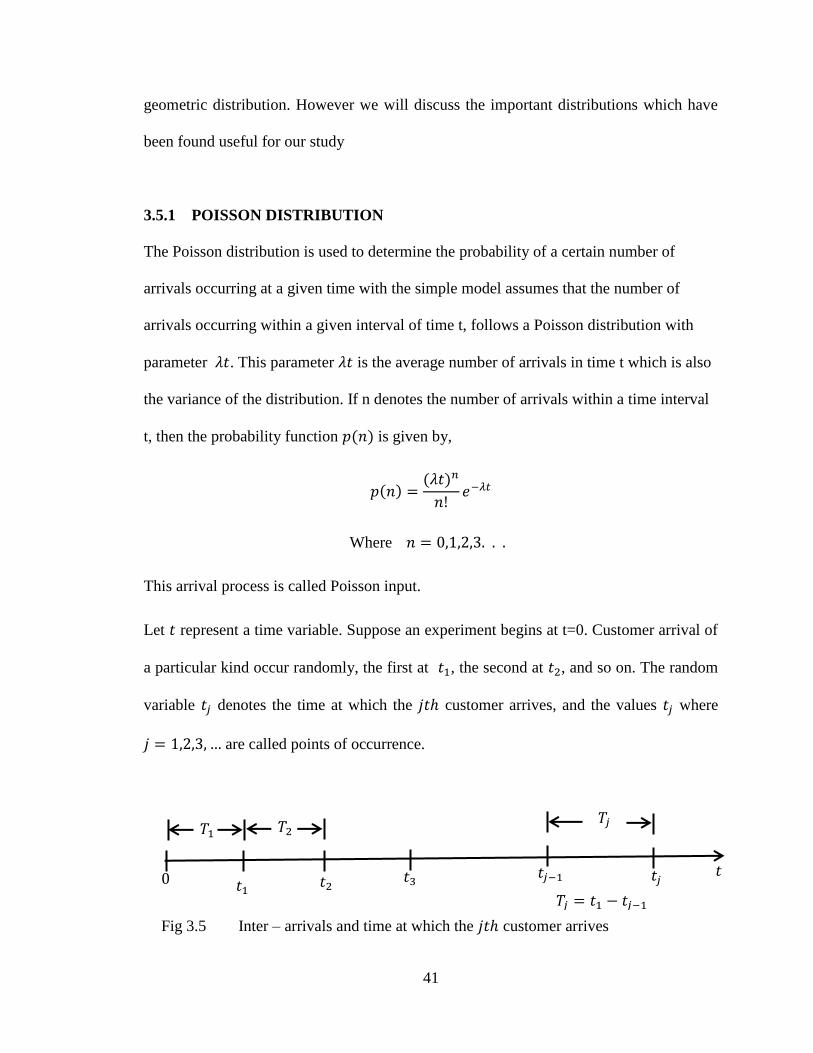
Let represent a time variable. Suppose an experiment begins at t=0. Customer arrival of

a particular kind occur randomly, the first at , the second at , and so on. The random

variable denotes the time at which the customer arrives, and the values where

are called points of occurrence.

Fig 3.5 Inter – arrivals and time at which the customer arrives

42

Let . For let donate the time between the and arrival. The

sequence of ordered random variables { } is called an inter arrival process as

shown in Fig 3.5

A stochastic process is a collection of random arrival times that describes the evolution of

some system over time. This process ( ), is said to be a counting process if

represents the total number of customer arrivals that have occurred up to time

. A counting process must satisfy:

a. ( ) and

b. is the integer valued

c. If then where is the time until the next arrival

d. For , the number of arrivals that have occurred

in the interval .

A counting process is said to have independent increments if the number of arrivals that

occur in disjoint time intervals are independent. For example and ( )

( ) are independent

A counting process ( ) is said to a Poisson process having random selection

of interval arrival time, T in a time interval , T from the

probability of having n points with an arrival rate 𝜆, 𝜆 , if

a. i.e. when arrival enters an empty queue

b. The process has independent increments.

43

c. The number of arrivals in any interval of length is Poisson distributed with mean

𝜆 . That is for all .

Then the probability of non (zero) arrival in the interval [0, t] is,

[ ]

Also, [ ]

From this it can be shown that the probability density function of the inter-arrival times

is given by,

This called the negative exponential distribution with parameter λ or simply

exponential distribution. The mean inter-arrival time and standard deviation of this

distribution are both 𝜆 where, 𝜆 is the arrival rate.

i.e.

Thus, the mean inter arrival time t is the reciprocal of the arrival rate.

3.5.2 EXPONENTIAL DISTRIBUTION

The most commonly used queuing models are based on the assumption of exponentially

distributed service times and inter arrival times.

The exponential distribution with parameter is given by for . If T is a

random variable that represents inter-service times with exponential distribution,

then

44

The cumulative distribution function of T is

The density function of inter – arrival times is

{

The expected time of inter – arrival is given by

∫

∫

By using integration by parts

[

|

∫

]

*

|

*

+

+

[

]

[

]

The exponential distribution has the interesting property that its mean is equal to its

standard deviation

3.5.3 GEOMETRIC DISTRIBUTION

The geometric (p) is used to indicate that the random variable X has the geometric

distribution with real parameter p satisfying 0 < p < 1. A geometric random variable X

with parameter p has probability mass function f (x) = p(1− p)x x = 0,1,2, . . . .

45

The geometric distribution can be used to model the number of failures before the first

success in repeated mutually independent Bernoulli trials, each with probability of

success p. The geometric distribution is the only discrete distribution with the

memoryless property. The only continuous distribution with the memoryless property is

the exponential distribution.

3.6 SERVER (TELLER) UTILIZATION FACTOR (

If the queuing system consists of a single server then, the utilization or the steady state

is the fraction of the time in which the server is busy that is occupied to the arrival. In

case when the source is infinite and there is no limit on the number of customer in the

single server (teller) queue, the server utilization is given by:

The steady state of a system with multiple servers is the mean fraction active servers. In

the above mention case since the number of servers is multiple, and then is the overall

services rate which implies

and can be used to formulate the condition for

stationary behaviour mentioned previously. The condition for stability is always between

zero and one. . If the utilization exceeds this range then the situation is

unstable and would need additional server(s). That is on the average the number of

customers that arrive in a unit of time must be less than the number of customers that can

be processed.

46

3.7 LITTLE’S LAW

According to Little (1961), The long-term average number of customers in a stable

system L, is equal to the long-term average arrival rate, 𝜆, multiplied by the long-term

average time a customer spends in the system, W; i.e. 𝜆

The relation between L and W is given by Little‘s Law. Let L be the average number of

customers in the system at any moment of time assuming that the steady – state has been

reached.

Consider a system from to the indefinite future and the values of the various

quantities of interest as time progresses which has a connection between average and

typical with the number of customers in the system, the customers delay and so on.

Let

= Number of customers in the system at time t

𝜆 = Number of customers who arrived in the interval [0, t]

= Time spent in the system by the arriving customer our intuitive notion of the

"typical" number of customers in the system observed up to time t is

∫

Where time average of up to time t. Naturally, changes with the time t, but in

many systems of interest, tends to a steady-state L as t increases, that is,

In this case, L the steady-state time average (or simply time average) of ).

It is also natural to view

𝜆

47

as the time average arrival rate over the interval [0,t] The steady-state arrival rate is

defined as

𝜆

𝜆

(Assuming that the limit exists) The time average of the customer delay up to time t is

similarly defined as

∑

that is, the average time spent in the system per customer up to time t. The steady-state

time average customer delay is defined as

(Assuming that the limit exists)

It turns out that the quantities L, 𝜆, and W above are related by a simple formula that

makes it possible to determine one given the other. This result, known as Little's

Theorem, has the form

𝜆

Little's Theorem expresses the natural idea that crowded systems (large W) are associated

with long customer delays (large W) and reversely. For example, on a rainy day, traffic

on a rush hour moves slower than average (large W), while the streets are more crowded

(large L). Similarly, a fast-food restaurant (small W) needs a smaller waiting room (small

L) than a regular restaurant for the same customer arrival rate.

In addition for the average number of customers in the queue at time t is given by

𝜆

and the average number of customers in the service at time t

48

𝜆

3.8 NOTATION FOR QUEUES.

Since all queues are characterized by arrival, service and queue and its discipline, the

queue system is usually described in shorten form by using these characteristics. The

general notation is:

[ ]

Where,

A = Probability distribution of the arrivals

B = Probability distribution of the departures

s = Number of servers (channels)

d = The capacity of the queue(s)

e = The size of the calling population

f = Queue ranking rule (Ordering of the queue)

There are some special notation that has been developed for various probability

distributions describing the arrivals and departures. Some examples are arrival or

departure distribution that is a Poisson process, Erlang distribution, General distribution,

General independent distribution etc.

Thus for example, the [M/M/1]:{infinity/infinity/FCFS} system is one where the arrivals

and departures are a Poisson distribution with a single server, infinite queue length,

calling population infinite and the queue discipline is FCFS. This is the simplest queue

49

system that can be studied mathematically. This queue system is also simply referred to

as the M/M/1 queue. Banking queues possess the Markovian Memoryless properties,

therefore in this study the focus will be on and to estimate the number

of servers needed during each time interval.

As we have stated earlier about the three main queuing systems in the case of study, that

is Single Server with Single Queue, Multiple Server with Single Queue, and Multiple

Single Server with Single Queue in Parallel, with models of the queues using

and . In these models an arrival occurs according to Poisson process in which the

input implies that arrivals are independent of one another or the state of the system. The

probability of an arrival in any interval of time does not depend on the starting point of

the arrival or on the specific history of arrivals preceding it, but depends only on the

length which is the property of Stationarity and Lack of Memory. These two assumptions

are often called Markovian, hence the use of the two ― ‖ in the notation used for the

models.

3.8.1 MODEL

It is the simplest realistic queue which assumes the arrival rate follows a Poisson

distribution and the time between arrivals follows an exponential distribution, has only

one server, with infinite system capacity and population, and with First-In, First –Out

(FIFO) as its queuing discipline.

Consider a single stage queuing system where the arrivals are according to a Poisson

Process with average arrival rate 𝜆 per unit time. That is, the time between arrivals is

according to an exponential distribution with mean

.

50

For this system the service times are exponentially distributed with mean

and there is a

single teller. The service rate must be greater than the arrival rate, that is 𝜆. If

λ, the queue would eventually grow infinitely large.

Considering the arrival and departure time in the system which can be applied in a variety

of areas, as ―birth‖ refers to the arrival of a customer while ―death‖ refers to the departure

of a customer called Birth and Death Process.

In this case both the inter-arrival times and the service times are assumed to be negative

exponential distribution with parameters λ and μ. As with Markovian process, the steady

state probability is the probability that in the long run there will be exactly j customers

in the system and how is determined for an arbitrary birth – death process.

The key is a small change using the analogy of Markov chains in

obtaining the flow balance equation or the conservation of flow equations for the birth –

death process (Winston 1994).

Consider figure 3.5 showing a state transitional rate diagram for single teller possessing a

model.

1

2

3

0

1

2

0 1 2

0

2

j+1

1

2

3

1

j-1 j

Figure 3.6 State Transitional rate diagrams for a single server

possessing

51

It follows that for equilibrium, the expected number of departures from the state j is equal

to the expected number of entrances into state j.

Thus, Expected rate in (arrivals)= Expected rate out (departures) principle …...(3.8.1-1)

Assuming the system settles down into the steady state, the system spends a fraction

of its time in state j. For , a customer can only leave state by going to state

or , so for , to get

𝜆 ………….……. (3.8.1-2)

Since for , a customer can only enter state then,

𝜆 (3.8.1-3)

By substituting equation ( 2 ) and ( 3) into equation ( 1 ),

it implies that

(𝜆 ) 𝜆

But for it implies that

Then it implies 𝜆

Steady state probability of being in state is

𝜆

𝜆 𝜆

𝜆 𝜆

𝜆 𝜆

𝜆 𝜆

52

Putting all together

𝜆 , 𝜆 , . . ., 𝜆 and

, (

)

. . ., (

)

Since the sum of all probabilities is equal to one, it implies

∑

⇒ ∑ (𝜆

)

⇒

∑ (𝜆 )

𝜆

∑ (

𝜆

)

∑

Therefore, the probability of any given number of customers being in the system is

∑

And is the steady state probability of state .

If , then it must be that 𝜆 and if the arrival is greater than the service rate, then

the state of the system will grow without end

With the steady-state probability for this system calculated, L can now be solved. If L is

the average number of customers present in the system, waiting to be served.

This is represented by the formula,

∑

∑

∑

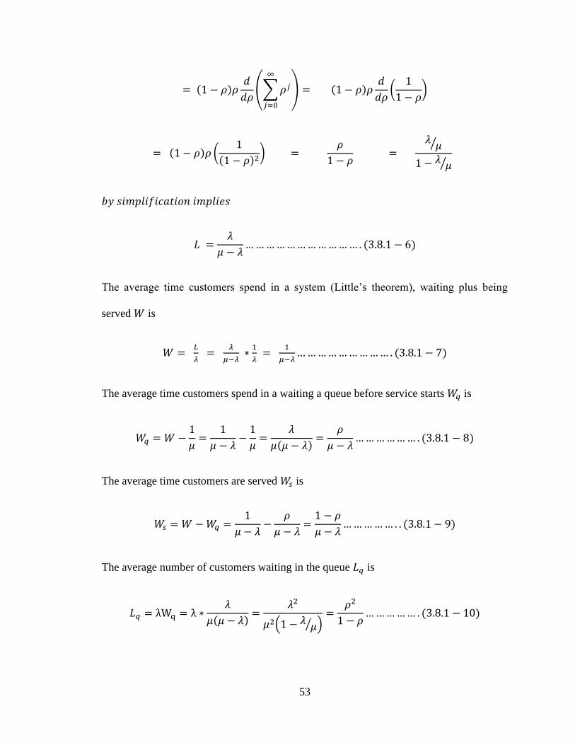
53

(∑

)

(

)

(

)

𝜆 ⁄

𝜆 ⁄

𝜆

𝜆

The average time customers spend in a system (Little‘s theorem), waiting plus being

served is

The average time customers spend in a waiting a queue before service starts is

𝜆

𝜆

𝜆

𝜆

The average time customers are served is

𝜆

𝜆

𝜆

The average number of customers waiting in the queue is

𝜆

𝜆

𝜆

( 𝜆 ⁄ )

54

To solve for , the number of customers that are in the service at any given moment is

determined. In this particular system, there will be one customer in service except for

when there are no customers in the systems. Thus, it can be calculated as follows

From these formulas one can conclude how busy the server is, by just watching the length

of the queue.

Illustrative example

A bank consisting of only on window, a solitary employee performs all the service

required and the window remains continuously open from 7am to 1pm. It has been

discovered that an average number of clients are 54 during the day and the average

service time is 5mins / person. Then the following can be known, the utilization factor,

average number of clients in the system, average waiting time etc.

Average number of client (arrival) = 54

Average service time per person = 5 minutes

Time ( 7am to 1pm) = 6 hours

Implies that the mean arrival rate 𝜆

and mean service rate

The utilization factor

It implies 𝜆 and

Average number of customer in the system

55

𝜆

𝜆

𝜆

𝜆

𝜆

𝜆

Average waiting time in a queue

𝜆

𝜆

𝜆

𝜆 𝜆

Average waiting time in a system

Average time customers are served

𝜆

The number of customers in the system at any given moment

𝜆

56

3.8.2 MODEL

The description of a queue is similar to that of the classic queue with the

exception that there are servers. When , all the results for the queue can

be obtained. The number of customers in the system at time , in the queue

can be modelled as a continuous Times Markov Chain.

The condition for stability is

where is called the service utilization factor,

the proportion of time on average that each server is busy. The total service rate must be

greater than the arrival rate, that is 𝜆, and if 𝜆 the queue would eventually

grow infinitely large.

Consider figure 3.6 showing a state transitional rate diagram for a multiple server

possessing a model.

Thus, Expected rate in (arrivals) = Expected rate out (departures) principle…...(3.8.2-1)

Assuming the system settles down into the steady state, the system spends a fraction

of its time in state j. For , a customer can only leave state by going to state

or , so for , to get

𝜆 …………….

Figure 3.7 State Transitional Rate diagram for a multiple

server possessing

3

1

2

(j-1)

3

2

0

1 2

0

2

j+1

j j j

1

j-1 j

0

1

0

57

Since for , a customer can only enter state then,

𝜆 ………………………………………

By substituting equation ( 2 ) and ( 3) into equation ( 1 ),

it implies that

(𝜆 ) 𝜆

But for it implies that

Then it implies 𝜆

Steady state probability of being in state is

𝜆

𝜆 𝜆

𝜆 𝜆

𝜆 𝜆

𝜆 𝜆

Putting all together

𝜆 , 𝜆 , 𝜆 , . . ., 𝜆

,

. . .,

58

,

(

)

(

) . . .,

…

,

(

)

(

)

. . .,

(

)

,

….,

(

)

where

And in general,

(

)

Since

∑

⇒ ∑

(𝜆

)

⇒

∑ (

𝜆 )

𝜆

∑

(

𝜆

)

∑

If there are more customers in the system, all the servers ―s‖ remain busy and

each is of the mean , and hence the mean service rate is . On the other hand, if there

are fewer customer than ―s‘ in the system, , only of the servers are busy and thus

the mean rat is . Hence {

The probability that at any given time there are customers in the system at any given

time from

(

) , then the steady solution is

59

{

(𝜆

)

(𝜆

)

The probability of any given number of customers being in the system is given

follows from normalization, yielding

(∑

𝜆

)

𝜆

⁄

⁄ 𝜆

⁄

(∑

)

The probability that at any given time there are no customers waiting or being served at

steady state

(∑

)

The expression for the average waiting time and queue lengths are fairly complicated and

depend on the probability of the average number of customers waiting in queue to be

served

∑

60

∑

𝜆 ⁄

𝜆 ⁄

∑

(𝜆 ⁄ )

(𝜆 ⁄ )

(

𝜆 ⁄ )

𝜆

The average number of customers in service

∑ ∑

Now, the average number of customers in the system becomes

𝜆

The average time customer spend in waiting in queue before service starts is

𝜆

The average time customer spend in the system, waiting plus being served is

𝜆

𝜆

𝜆

𝜆

The average time customers are served (

)

61

Illustrative example

A commercial bank has 3 servers assisting customers and the customers are found to

arrive in a Poisson distribution at an average of 6 customers per hour for the business

transaction. The service time is found to have an exponential distribution with mean of 18

minutes. The customers are processed on FCFS. In this situation the average queue length

, the average number of customers in the queue , the average time a customer spends

in the queue , and the average number of customers in the serves can be known.

It implies that 𝜆 and

Service utilization factor

For The probability that at any given time there are no customers waiting

(∑

)

(∑

)

(

)

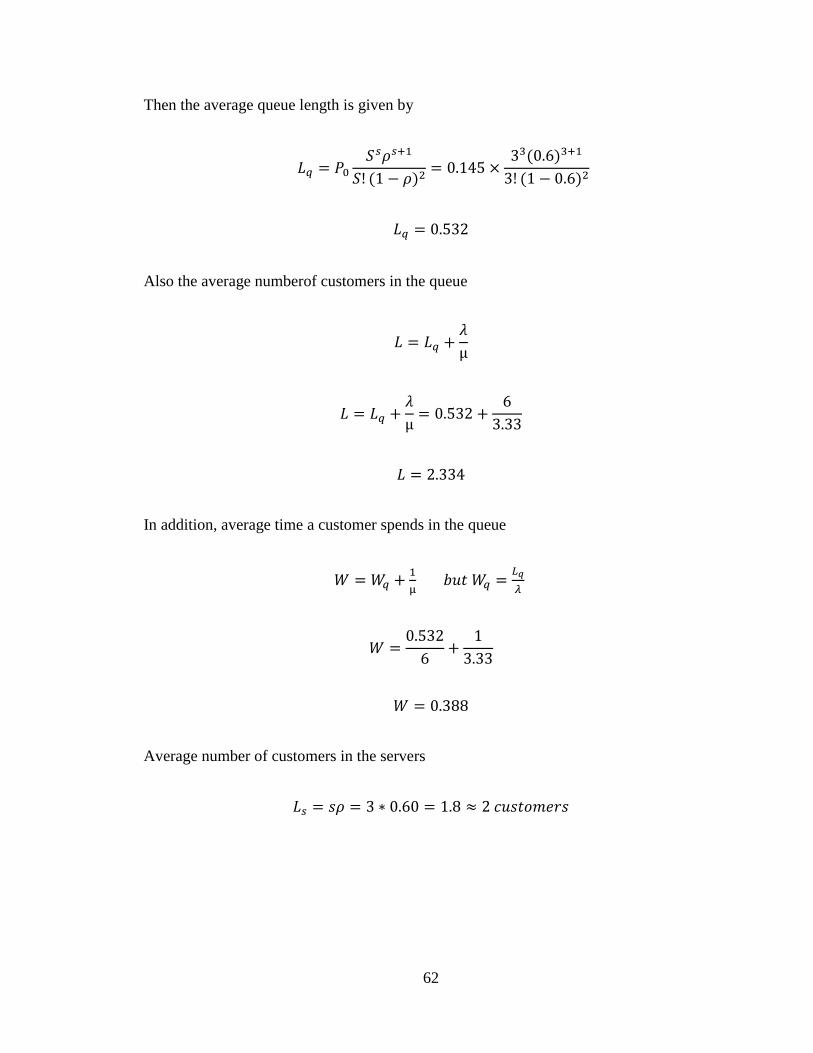
62

Then the average queue length is given by

Also the average numberof customers in the queue

𝜆

𝜆

In addition, average time a customer spends in the queue

Average number of customers in the servers

63

CHAPTER FOUR

DATA ANALYSIS AND DISCUSSION OF RESULTS

4.0 INTRODUCTION

This chapter introduces the analysis of the model and discussion of findings. Preliminary

analysis, summary of results and snapshot of the data will also be presented and

discussed.

The queuing model used in the analysis is which involves a single-line with

multiple servers in the system.

The following assumptions are made:

1. The customers face balking, reneging, or jockeying and come from a population that

can be considered as infinite.

2. Customer arrivals are described by a Poisson distribution with a mean arrival rate of 𝜆

(lambda). This means that the time between successive customer arrivals follows an

exponential distribution with an average of 𝜆.

3. The customer service rate is described by a Poisson distribution with a mean service

rate of µ (mu). This means that the service time for one customer follows an exponential

distribution with an average of 1/µ.

4. The waiting line priority rule used is first-come, first-served.

Using these assumptions, we can calculate the operating characteristics of a waiting line

system.

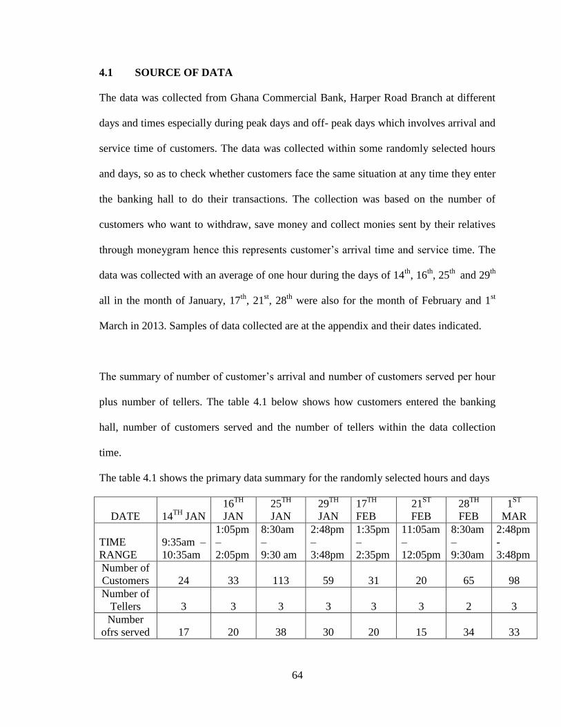
64

4.1 SOURCE OF DATA

The data was collected from Ghana Commercial Bank, Harper Road Branch at different

days and times especially during peak days and off- peak days which involves arrival and

service time of customers. The data was collected within some randomly selected hours

and days, so as to check whether customers face the same situation at any time they enter

the banking hall to do their transactions. The collection was based on the number of

customers who want to withdraw, save money and collect monies sent by their relatives

through moneygram hence this represents customer‘s arrival time and service time. The

data was collected with an average of one hour during the days of 14th

, 16th

, 25th

and 29th

all in the month of January, 17th

, 21st, 28

th were also for the month of February and 1

st

March in 2013. Samples of data collected are at the appendix and their dates indicated.

The summary of number of customer‘s arrival and number of customers served per hour

plus number of tellers. The table 4.1 below shows how customers entered the banking

hall, number of customers served and the number of tellers within the data collection

time.

The table 4.1 shows the primary data summary for the randomly selected hours and days

DATE 14TH

JAN

16TH

JAN

25TH

JAN

29TH

JAN

17TH

FEB

21ST

FEB

28TH

FEB

1ST

MAR

TIME

RANGE

9:35am –

10:35am

1:05pm

–

2:05pm

8:30am

–

9:30 am

2:48pm

–

3:48pm

1:35pm

–

2:35pm

11:05am

–

12:05pm

8:30am

–

9:30am

2:48pm

-

3:48pm

Number of

Customers 24 33 113 59 31 20 65 98

Number of

Tellers 3 3 3 3 3 3 2 3

Number

ofrs served 17 20 38 30 20 15 34 33

65

The table above summarizes all data collected. The collection of data was done within an

hour. During the peak days, that is on the 25th

, 29th

of January and the 28th

and 1st of

March saw many customers arrive at the banking hall. Due to the payment of salaries and

other transactions around these times of the month, a lot of customers troop into the

banking halls to collect their salaries and other services. Consequently, pressure is

exerted on the network servers culminating into breakdown of services due to the

unstable nature of the network. Customers therefore, complain bitterly about the service

operations of the bank during these peak periods. On the other hand, there is less pressure

on the network during the off peak days due to minimal arrival of customers into the

banking hall. Hence network problems were rarely experienced during these periods.

4.2 DESCRIPTIVE ANALYSIS OF DATA

During the collection of the data it was found out that customers entered the banking hall

frequently on specific dates and less frequently on some other dates within the month. A

graph which depicts sample of the arrival time of both peak and off-peak days was

plotted with number of customers against arrival time. From the graph customers‘

number begins from 0 to j, which means that during peak periods customers come to the

banking hall frequently as compared to the off-peak days. Figure 4.1 shows a graph of the

number of customers arriving at a banking hall against their respective arrival time.

Arrival of Customers and Time on Peak days (25th and 29th) and off-peak (14th and

15th), from figure 4.1 it can be seen that on the 25th and 29th more customers trooped

into the banking hall for payment of salaries, school fees and money transfer as it‘s a

normal practice around that time of the month.

66

Figure 4.1 A Graph Show the Arrival of Customers

In addition, during the peak period‘s customers were confronted with jockeying,

reneging or balking due to the long queues, long wait, network problems, slowness of a

teller and bad attitude on the side of a staff. It was also noticed some customers were

irritated due to fact that others were attended to without joining the queue by virtue of

them being friends of the tellers. Some tellers practically vacated their cubicles leading to

customers complaining as their waiting time kept rising higher than they anticipated

because they assume that their waiting time was higher than expected.

4.3 PARAMETERS FROM DATA

Throughout the analysis, an hour (01:00:00) will be taking as 1.00, in order to have

simple average calculations. The rate of customer arrival at the banks fluctuates

0:00:00

0:07:12

0:14:24

0:21:36

0:28:48

0:36:00

0:43:12

0:50:24

0:57:36

1:04:48

1 6

11

16

21

26

31

36

41

46

51

56

61

66

71

76

81

86

91

96

10

1

10

6

11

1

Arr

ival

Tim

e

Number of Customers arriving

14th Jan

16th Jan

25thJan

29th Jan

67

throughout the day and there might be differences in arrival from day to day but we

assume that they are independent and identically distributed.

4.3.1 FROM TABLE 4.1, ON THE 14TH

OF JANUARY THE DATA

COMPUTATION

The number of customers entering the bank (Arrival rate) = 24

The number of customers served within 9:35am – 10:35am (service rate ) = 17

The number of tellers = 3

Total time spent in hours = 1 hr

Mean arrival rate 𝜆

Mean service rate

The summary of parameters from data that was used in the analysis, the table consists of

mean arrival rate, mean service rate, number of tellers and total time spent.

The table 4.2 shows the parameter from data summary for the randomly selected hours

and days

DATE

14TH

JAN

16TH

JAN

25TH

JAN

29TH

JAN

17TH

FEB

21ST

FEB

28TH

FEB

1ST

MAR

Total Time 1 1 1 1 1 1 1 1

Mean

Arrival Rate 24 33 113 59 31 20 65 98

Mean

Service Rate 17 20 38 30 20 15 34 33

Number of

Tellers 3 3 3 3 3 3 2 3

Summary of Data Collected

68

4.4 COMPUTATIONAL PROCEDURE

A Core i5 Toshiba Satellite S855 – S5369 laptop was used for the data computation. The

model was Inter ® Core ™ i5 CPU with a speed of 6 gigabytes. It has a hard disk size of

640 gigabytes with Random Access Memory of 4 gigabytes.

An excel solver was used to for the computation.

4.5 RESULTS

Results for sample computation are shown below for the data of 14th

January, 2013. The

results for other dates follow similar calculations using excel solver.

1. Utilization factor for 14th

January is given by:

2. The probability that at any given time the system will be idle (there are no customers

waiting).

(∑

)

(∑

)

(

)

69

3. Probability of an average number of customers waiting in queue to be served

4. The average number of customers in the system

𝜆

5. The average time customer spend in waiting in queue before service starts is

𝜆

6. The average time customer spend in the system, waiting plus being served is

70

7. The average time customers are served

The results show that the server would be busy 47.06% of the time and idle 23.29% of

the time. Also, the average number of customers in the waiting queue is 0.1834 and the

average number of customers waiting in the system is 1.5882. More so, the average time

a customer spends in the queue is 0.0076 hours and average a customer spends in the

system is 0.05882 hours.

4.5.1 RESULTS SUMMARY

From table 4.1 the data was analysis by the use of excel as shown in the appendix with its

formulas in which the results show the dates in which the data was collected, inputs,

intermediate calculation and performance measures. The results are as follows in the

table below

71

Table 4.3. Presentation on data analysis form table 4.2

BANK GHANA COMMERCIAL BANK, HARPER ROAD, KUMASI

DATE 14TH JAN 16TH JAN 25TH JAN 29TH JAN 17TH FEB 21ST FEB 28TH FEB 1ST MAR

UNITS INPUTS

Total Time Involved (t) 1.00 1.00 1.00 1.00 1.00 1.00 1.00 1.00 hours

Number of Customers Arrived 24 33 113 59 31 20 65 98 Customers

Number of Customers Served 17 20 38 30 20 16 34 33 Customers

Number of Servers 3 3 3 3 3 3 2 3 Servers

Model Type M/M/3 M/M/3 M/M/3 M/M/3 M/M/3 M/M/3 M/M/2 M/M/3

Intermediate Calculations

Average Arrival Rate 0.0417 0.0303 0.0088 0.0169 0.0323 0.0500 0.0154 0.0102

Average Serve Rate 0.0588 0.0500 0.0263 0.0333 0.0500 0.0625 0.0294 0.0303

Performance Measures

Rho(average server utilization) 0.4705 0.5500 0.9912 0.6555 0.5167 0.4167 0.9559 0.9899

Probability of System empty 0.2329 0.1762 0.00197 0.1165 0.1986 0.2786 0.0226 0.0023

Average Customers in the sys. L 1.5951 2.0083 114.1063 2.7830 1.8226 1.3611 22.1554 99.1056

Average Customers waiting in a

queue Lq 0.1843 0.3583 111.1326 0.8163 0.2726 0.1111 20.2436 96.1359

Average customer‘s wait in the

System Ls 1.3333 1.6500 2.9737 1.9667 1.5500 1.2500 1.9118 2.9697

Average time in the system, W 0.0664 0.0609 1.0098 0.0472 0.0588 0.0681 0.3409 1.0113

Average time in the queue, Wq 0.0076 0.0109 0.93835 0.0138 0.0088 0.0056 0.3114 0.9810

Average time a Customer is

served, Ws 0.05882 0.0500 0.0263 0.0333 0.0500 0.0625 0.0294 0.0303

72

4.5.2 RESULTS FOR AVERAGE DATA

The total number of customers observed was 443, out of that 208 was served and it a total

of 8 hours with a maximum of 3 tellers or servers. The table below shows the

intermediate calculations and performances measures.

Table 4.4 Average Data Calculation Results

INPUTS

Total Time Involved (t) 8 hours

Number of Customers Arrived 443

Number of Customers Served 208

Number of Servers 3

Model Type m/m/3

Intermediate Calculations

Average Arrival Rate 0.002257

Average Serve Rate 0.004808

Performance Measures

Rho(average server utilization) 0.6933

Probability of System empty 0.1287

Average Customers in the sys. L 30.6180

Average Customers waiting in a queue Lq 25.4727

Average customer‘s wait in the System Ls 1.9507

Average time in the system, W 0.3329

Average time in the queue, Wq 0.2847

Average time a Customer is served, Ws 0.4257

The results show that the server would be busy 69.33% of the time and idle 12.87% of

the time. Also, the average number of customers in the waiting queue is 25.47 and the

average number of customers waiting in the system is 30.612. More so, the average time

a customer spends in the queue is 0.2847 hours and average a customer spends in the

system is 0.3329 hours.

Analysis of results generated from the excel solver is presented in table 4.4; the data

analysis is as follows:

73

Utilization factor helps to determine how busy the tellers or servers are as shown

in the table below

From Table 4.5, the busiest of all the days is 25th

of January. Its utilization factor is

99.12% followed by 1st March with a utilization factor of 98.99%. On the 21

st of

February recorded the least of 41.67%. On the average, the utilization factor for all the

days was 69.33% from table 4.4. The days with higher utilization factor recorded a high

turnout of customers and vice versa.

Probability of the system being empty is the relative frequency with which the

service system is empty or idle. Idle time is directly related to cost.

From table 4.6, the probability of the system being empty implies that no customer will

be in the system to be served. The greater the probability the faster the system will

become empty. On the average, the probability of the system is 0.12871 from table 4.4.

And the greater the probability for which the system will be is 0.2786 which occurred on

Table 4.5 Utilization Factors For Each Day

DATE 14TH

JAN 16TH

JAN 25TH

JAN

29TH

JAN 17TH

FEB 21ST

FEB 28TH

FEB 1ST

MAR

Rho(average server

utilization) 0.4705 0.5500 0.9912 0.6555 0.5167 0.4167 0.9559 0.9899

Table 4.6 The Probability of the System Being Empty Or Idle

DATE 14TH

JAN 16TH

JAN 25TH

JAN

29TH

JAN 17TH

FEB 21ST

FEB 28TH

FEB 1ST

MAR

Probability of

System empty 0.2329 0.1762 0.0020 0.1165 0.1986 0.2786 0.0226 0.0023

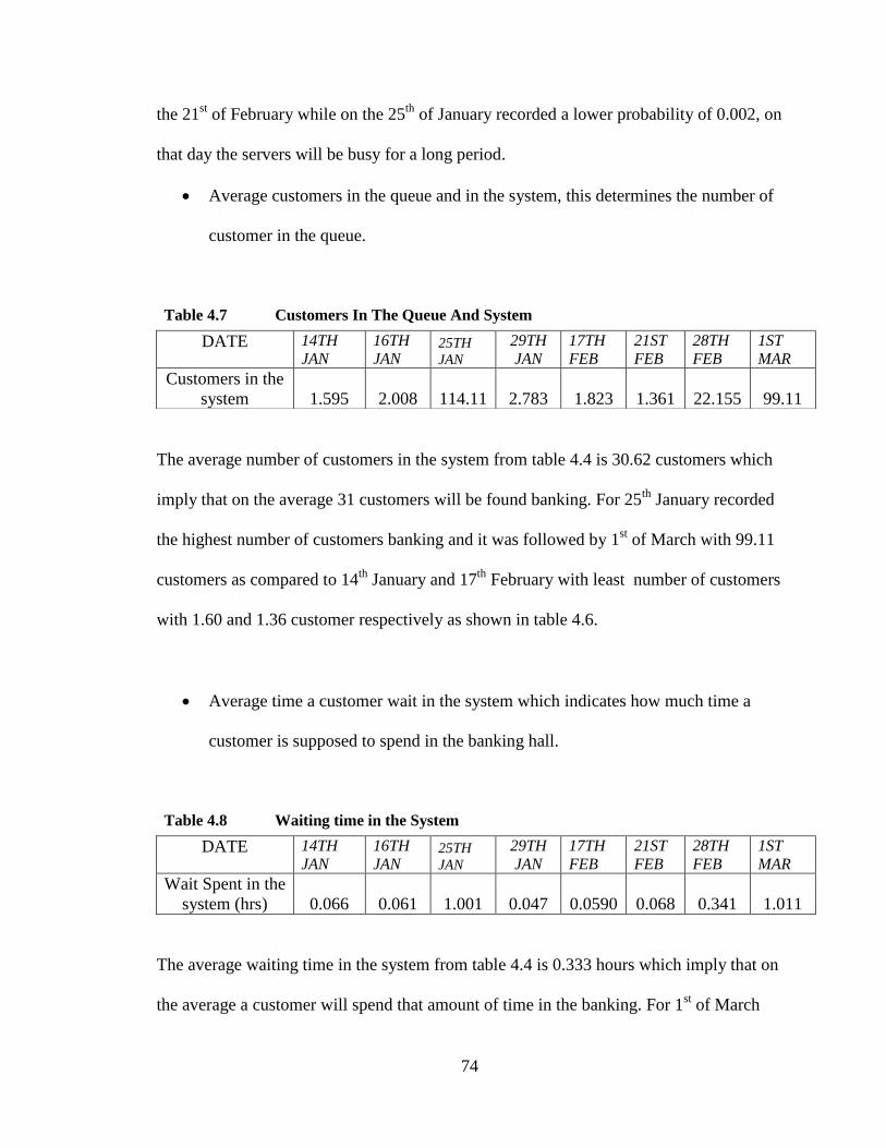
74

the 21st of February while on the 25

th of January recorded a lower probability of 0.002, on

that day the servers will be busy for a long period.

Average customers in the queue and in the system, this determines the number of

customer in the queue.

The average number of customers in the system from table 4.4 is 30.62 customers which

imply that on the average 31 customers will be found banking. For 25th

January recorded

the highest number of customers banking and it was followed by 1st of March with 99.11

customers as compared to 14th

January and 17th

February with least number of customers

with 1.60 and 1.36 customer respectively as shown in table 4.6.

Average time a customer wait in the system which indicates how much time a

customer is supposed to spend in the banking hall.

The average waiting time in the system from table 4.4 is 0.333 hours which imply that on

the average a customer will spend that amount of time in the banking. For 1st of March

Table 4.7 Customers In The Queue And System

DATE 14TH

JAN 16TH

JAN 25TH

JAN

29TH

JAN 17TH

FEB 21ST

FEB 28TH

FEB 1ST

MAR

Customers in the

system 1.595 2.008 114.11 2.783 1.823 1.361 22.155 99.11

Table 4.8 Waiting time in the System

DATE 14TH

JAN 16TH

JAN 25TH

JAN

29TH

JAN 17TH

FEB 21ST

FEB 28TH

FEB 1ST

MAR

Wait Spent in the

system (hrs) 0.066 0.061 1.001 0.047 0.0590 0.068 0.341 1.011

75

recorded the highest waiting time spent in the banking hall with 1.011 and it was

followed by 25th

January with 1.001 customers as compared to 29th

and 16th

all in

January had the least waiting time in the system with 0.047 and 0.061 hours respectively

as shown in table 4.7.

4.6 EFFECT OF UTILIZATION FACTOR

The entire utilization factors for the data are stable, utilization factor how much time the

tellers are busy or working and the waiting time that is how long do customers wait

before services? These two items are conflicted that is as utilization ( decreases,

waiting time also decreases and as it increases waiting time also increases. The average

of the utilization factor for all the dates that is 0.6933The highest utilization factor was

0.99122 on the 25th

of January, which is followed by 0.9898 also on the 1st of March and

0.95588 also on the 28th

of February all happen during the peak days. We noticed that

these entire high utilization factors also recorded a high waiting time during those periods

which are 1.0097905, 1.011281557 and 0.34085213 respectively.

Considering the data collected and through observation at the bank all the average

arriving rates are greater the average service rate, it was also noticed that the closer the

average service rate to the average arriving rate, the smaller utilization factor becomes

and the least waiting time. As the tellers were dispensing their duties, it was found out

that on the 21ST

of February, 2013 was at its best when it recorded a lowest capacity

utilization of 0.4167 with its arrival rate of 20 customers and out of that 16 customers

were served. On the 25th

of January, 2013 also recorded the highest capacity of utilization

76

of 0.9912 with an arrival of 113 customers and out of that 33 were served at the time all

the tellers were available with the hours the data was collected. This implies that the

tellers were on their best on that day and managed to serve many customers as possible

and when the number of tellers decreases, the higher the utilization factor gets closer to

one.

4.7 THE PROBABILITY OF THE SYSTEM BEING EMPTY

The probability of the system being empty is characterized by how busy the tellers are

working, the Table 4.3 shows the highest and lowest probability of the system being

empty, the utilization factor and the length of the queue as well their following dates

during the period of data collection.

The smaller the probability of the system being empty, the greater capacity of utilization

factor or increases, and the higher the probability of the system being empty and the

smaller the utilization factor and the number of customers in the entire queuing system

approaches zero. The highest probability for the system to be empty occurred on the 21ST

of February which is 0.27860 and on the 25th

of January recorded the lowest probability

of the system being empty which is 0.00196,

4.8 RELATIONSHIP BETWEEN HIGHEST AND THE LEAST NUMBER OF

CUSTOMERS ARRIVAL

Considering the highest arrival number of customers (113 customers) that was on the 25th

of January and the least arrival number of customers (20 customers) that was on the 21ST

of February the for peak and off – peak day respectfully. We observe that there is huge

77

difference between their capacity utilization factor the two is 0.99123 and 0.41667 and

the probability of the number of customers in the system to be empty is 0.00197 and

0.27861 respectively. This means that, there will be 114.1063 and 1.36105 average

number of customers in the system and would take 1.00979 and 0.06805 hour(s) average

time to be in the system respectively

4.9 PROJECTIONS USING 28TH

FEBRUARY 2013

Now let us consider one of the days in which the banking industry having recorded

capacity utilization closer to total average server utilization and total average customers

in the systems. Studying the performance analysis assuming there is one teller, two

tellers, three tellers, two tellers and five tellers and compare their results to make policy

recommendation. Taking an average arrival rate, 𝜆 and service rate, on the

28th

February was used for this analysis. The table 4.8 presents the results for considering

one to five tellers at a given time using the inputs obtained on the 28th

February, 2013.

Table 4.9 Shows Results of Types Models from One to Five Tellers at a Given Point.

TYPES OF MODEL M/M/1 M/M/2 M/M/3 M/M/4 M/M/5

Performance Measures

Rho(average server utilization) 1.91176 0.95588 0.63725 0.47794 0.38235

Probability of System empty -0.91176 0.02256 0.12579 0.14348 0.14695

Average Customers in the system L -2.09677 22.15539 2.62121 2.05180 1.94311

Average Customers waiting in the queue

Lq -4.00854 20.24362 0.70945 0.14004 0.03134

Average customers waiting in the System

Ls 1.91176 1.91176 1.91176 1.91176 1.91176

Average time in the system, W -0.03226 0.34085 0.04033 0.03157 0.02989

Average time in the queue, Wq -0.06167 0.31144 0.01091 0.00215 0.00048

Average time a Customer is served, Ws 0.02941 0.02941 0.02941 0.02941 0.02941

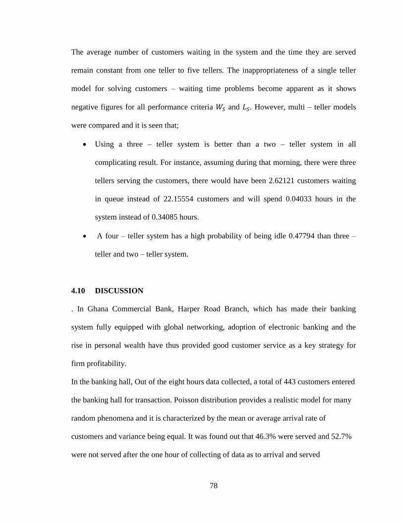
78

The average number of customers waiting in the system and the time they are served

remain constant from one teller to five tellers. The inappropriateness of a single teller

model for solving customers – waiting time problems become apparent as it shows

negative figures for all performance criteria and . However, multi – teller models

were compared and it is seen that;

Using a three – teller system is better than a two – teller system in all

complicating result. For instance, assuming during that morning, there were three

tellers serving the customers, there would have been 2.62121 customers waiting

in queue instead of 22.15554 customers and will spend 0.04033 hours in the

system instead of 0.34085 hours.

A four – teller system has a high probability of being idle 0.47794 than three –

teller and two – teller system.

4.10 DISCUSSION

. In Ghana Commercial Bank, Harper Road Branch, which has made their banking

system fully equipped with global networking, adoption of electronic banking and the

rise in personal wealth have thus provided good customer service as a key strategy for

firm profitability.

In the banking hall, Out of the eight hours data collected, a total of 443 customers entered

the banking hall for transaction. Poisson distribution provides a realistic model for many

random phenomena and it is characterized by the mean or average arrival rate of

customers and variance being equal. It was found out that 46.3% were served and 52.7%

were not served after the one hour of collecting of data as to arrival and served

79

customers. The average number of customers in an hour per the four days off – peak days

is 27 customers, and an average number of customers in an hour per day during a peak

day are 84 customers. It was equally observed that while some customers had to wait for

as much as two hours before service, some spent only two minutes. Introduction of an

additional server is capable of reducing loss of customers by 60% by other staffs who are

less busy becoming servers to help reduce the queue and get back to their work when the

length of the queue reduces. It was also noticed that friends of cashiers received quicker

service, at the expense of others and teller points were opened and closed at will leading

to customers confusion and complaints because their waiting time was higher than

expected. A four – teller system would be preferable than three and three and two – teller

system.

80

CHAPTER FIVE

CONCLUSION AND RECOMMENDATION

5.1 CONCLUSION

The objective of this study was to determine the amount of waiting time a customer is

likely to experience and how it will be affected if there are alterations in the facilities.

The study uncovered the applicability and extent of usage of queuing models in achieving

customer satisfaction at the lowest cost as well as permitting us to make better decisions

relating to tellers and potential waiting times for customers.

It is determined that customers spent more time at the banking hall of Ghana

Commercial Bank, Harper Road, Kumasi on peak day that is 1.0113 hours and on an off

peak day customers spend a minimum of 0.0472 hours. On the average day a customer

spends 0.3329 hours.

The average time a customer spends in the system for two servers is 0.34085 and 0.24033

hours for three servers. An increased in service unit to four servers would reduce the

average waiting time in the system drastically to 0.03157 hours. There should be more

tellers available to help ease build up queues since the banking hall has extra teller space

to avoid long queues at that period.

Loss of goodwill and withdrawal of accounts on the part of customers because of long

queues compensate for the cost of extra hand to be hired.

81

5.2 RECOMMENDATIONS

Based on the summary and conclusion of this study, the following recommendations

were made for efficient and quality service to customers of Ghana Commercial Bank, of

Harper Road-Kumasi.

1. The management should adopt a four - teller or five - teller model to reduce

waiting time at the banking hall during peak periods in other to increase customer

satisfaction.

2. A reduction in the number of tellers exerts unnecessary pressure at the banking

hall and the entire queuing system. Hence, increases the capacity of utilization on

the banking facilities. Whenever a teller is on break or leaves for other

transactions, especially at a peak period, the managers should replace them to

avoid time delays due to long queue of customers.

82

REFERENCES

1. Abor, J. (2004). Technological innovations and banking in Ghana: An evaluation of

customers‘ perceptions. American Academy of Financial Management, 1, 1-16. [Online]

Available: http://www.financialcertified.com/armstrong.html

2. Ankaah, K. N. (1995), Banks as providers of funds for building business,‖ The Ghanaian

Banker, Journal of the chartered Institute of Bankers Ghana. pp6

3. Agbadudu, A.B. (1996), Elementary Operation Research. Vol. I: Benin City, A.B. Mudiaga

Limited.

4. Alain Jean-Marie and Emmanuel Hyon, (2009). Scheduling in a queuing system with

impatience and setup costs, Theme COM – Systemes communicants Equipe-Projet Maestro,

Rapport de recherché 6881—Mars 2009—16 pages

5. Bhat, U. N.(2008) An Introduction to Queuing Theory: Modelling and Analysis in

Application (Statistics for Industry and Technology).

6. Bunday, B.D. (1996), An Introduction to Queuing Theory: New York: Halsted Press.

7. Chonggang Wang Bin Li ; Thomas Hou, Y. ; Kazem Sohraby and Yu Lin,( 2004). A

Robust Active Queue Management Scheme Based On Packet Loss Ratio infocom. Twenty-

third Annual Joint Conference of the IEEE Computer and Communications Societies.

Conference Publications

8. Coffman, E. G. Jr. and Hofri, M. (1986). ―Queueing models of secondary storage devices‖,

Queueing Systems, 1, 129-168.

9. Coffman, E. G. Jr. and Donning, P. J. (1973). Operating Systems Theory, Prentice Hall,

Englewood Cliffs, N.J.

10. Crowley, D., Bard, J., Jensen, P., (1995), Using flow ratio analysis and discrete event

simulation to design a medium volume production facility, Computers and Engineering

28(2): 379-397

83

11. Elegalam (1978) ―Customer retention versus cost reduction technique‖ a paper presented at

the Bankers forum held at Lagos, pg.9-10.

12. Estan, C and G. Varghese (2002), ―New directions in traffic measurement and accounting,‖ in

Proc. Acm Sigcomm, pp. 323–336

13. Filipowicz, B. and Kwiecień, J.(2008), Queueing systems and networks. Models and

applications Department of Automatics, AGH University of Science and Technology, 30

Mickiewicza Ave., 30-059 Kraków, Polan

14. Ghana Commercial Bank Limited Annual Report, 2010

15. Ghana Commercial Bank Limited Diary, 2008.

16. Giedrius M and Eimutis V. (2006), Modelling of Non-Markovian Queuing Systems; Dept of

Mathematical Research in Systems, Kaunas University of Technology, Studentų g. 50, 51368

Kaunas, Lithuania, accepted 20 November 2006

17. Gross, D. and Harris C.M. (1998), Fundamentals of Queuing Theory. New York: John Wiley

and Sons

18. Gurumurthi and Benjaafar (2004), Modeling and Analysis of Flexible Queuing Systems

Naval Research Logistics, Vol. 51 (2004), Wiley Periodicals, Inc.

19. Jacob M. (2009), Application of Multiserver Queuing To Call Centers a thesis submitted in

partial fulfilment of the requirements For Master of Science in mathematical statistics degree

in the faculty of science, Rhodes University Faculty of science Department of statistics.

20. Kinnis K. Gosha (2007), The Effects Of An Advance Queue Management System On

Barbershop Administration, Master of Science, May 10, 2007, Albany State University.

21. Kleinrock, L. (1976). Queueing Systems, Vol. II: Com-puter Applications. John Wiley, New

York.

84

22. Jong-hwan K., Hyunsoo Y., Ikjun Y. (2011), "Active Queue Management for Flow Fairness

and Stable Queue Length," IEEE Transactions on Parallel and Distributed Systems, vol. 22,

no. 4, pp. 571-579, April, 2011.

23. Kotler, P. (1999), Marketing Management, The New Millennium Edition.

24. Larson, R.C (1987), Perspectives on queues: social justice and the psychology of queuing.

Journal of Operation Research, 35, 895–905.

25. Lucas R. W. (2005), Customer Service ―Building Successful Skills for the Twenty-First

Century‖.Spain, Mc Graw-Hill Publishers.

26. Mandia S. (2006), Design of Queuing System ,Department of Mechanical and Industrial

Engineering

27. Marfo-Yiadom, E and Abraham (2012), A. Customers‘ Perception of Innovative Banking

Products in Cape Coast Metropolis, Ghana School of Business, University of Cape Coast

Cape Coast, Ghana

28. Michael, K. (2001), "Service on Call" in Banking Technology News Service Network,

http/www.fineos.com/documentation/features/bankreach.com.

29. Nafees A. (2007) Queuing Theory and its Application: Analysis of The Sales Checkout

Operation in ICA Supermarket , A ‗D level‘ essay in Statistics submitted in partial

fulfillment of the requirements for the degree of M. Sc. Department of Economics and

Society June 2007

30. Nosek, Jr., R. A. and Wilson, J. P. (2001) Queuing theory and customer satisfaction: a review

of terminology, trends, and applications to pharmacy practice. Hospital Pharmacy, 36, 275-

279

31. Olaniyi T.A. (2004) An appraisal of Techniques for minimizing cost of customers waiting in

first bank of Nigeria Plc Ilorin (An M.Sc. Seminars presentation to the Department of

Accounting & Finance Unilorin).

85

32. Osuagwu, L. (2002). Marketing Principle and Management. (2 nd edition) Lagos, Grey

Resource Ltd.

33. Paul E. Black,(2006) ―Queues‖ in dictionary of Algorithms and data structure, U.S National

Institute of Standars and Technology ,

34. Prabhu, N.U. (1997), Foundations of Queuing Theory: Ithaco, NY: Khuwar Academic

Publishers.

35. Prikryl J. and Kocijan J (2012), Stochastic Analysis of a Queue Length Model Using a

Graphics Processing Unit, Transactions On Transport Sciences Number 2, Volume 5 2012,

DOI: 10.2478/V10158-012-0007-2

36. Ronald A. N. and Wilson J. P, (2001) Queuing Theory and Customer Satisfaction: A Review

of Terminology, Trends, and Applications to Pharmacy Practice, Hospital Pharmacy Volume

36, Number 3, pp 275–279

37. Rongrong Z. and Dilip S (2003), Looking Back: Exploring the Psychology of Queuing and

the Effect of the Number of People Behind, 2003 by Journal of Consumer Research, Inc. ●

Vol. 29 ● March 2003, all rights reserved. 0093-5301/2003/2904-0005

38. Rouba I. and Ward W. (2009), Real-Time Delay Estimation in Overloaded Multiserver

Queues with Abandonments Management Science 2009 55:1729-1742; published online

before print July 20, 2009, doi:10.1287/mnsc.1090.1041

39. Stakutis C. and Boyle T. (2009). Your health, your way: Human-enabled health care. CA

Emerging Technologies, pp. 1-10.

40. Sokefun A. O,(2001). Customer Service and Its Effect on the Banking Business in Nigeria,

Redeemer‘s University Mowe, Ogun State. Department Of Financial Studies JORIND 9(2)

December, 2011. ISSN 1596 – 8308.

86

41. Tabari M, Gholipour-Kanani Y., Seifi-Divkolaii M. and Tavakkoli-Moghaddam R (2012).

Application of the Queuing Theory to Human Resource Management, World Applied

Sciences Journal 17 (9): 1211-1218, 2012, ISSN 1818-4952 © IDOSI Publications,

42. Turban, E., King D., Lee J., Warkentin M., and Chung H.M., (2002). Electronic Commerce:

A Managerial Perspective. New York, Prentice Hall

43. Udayabhanu, V, Sunder K. and Kannan S. (2010), Optimizing Capacity Utilization in

Queuing Systems: Parallels with the EOQ Model, California Journal of Operations

Management, Volume 8, Number 1, February 2010 CSU-POM

44. Vasumathi .A and Dhanavanthan P (2010)Application of Simulation Technique in Queuing

Model for ATM Facility International Journal Of Applied

Engineering Research, Dindigul Volume 1 , No 3, 2010 .

45. Vjacheslav Usmanov and Cenek Jarsky (2009); Application of queuing theory in construction

industry, Department of Construction Technology, FCE, CTU Prague, Czech Republic

46. Winston, W. L. (1994). Operations research: applications and algorithms. 3rd

ed. Duxbury

Press Belmont, Califonia. pp 1117-1121.

47. Zeithaml, V. (2000). Service Quality, Profitability and the Economic Worth of Customers:

What we Know and What we Need to Learn. Journal of Academy of Marketing Science,

28(1), 67. http://www.investopedia.com/terms/b/bank.asp#ixzz2A9byIi4N

87

APPENDICES

A.1.0 SAMPLE OF MICROSOFT OFFICE EXCEL SPREADSHEET

88

A.2.0 MICROSOFT OFFICE EXCEL SPREADSHEET FORMULAS

B 12 =1/B7

B 13 =1/B8

B 14 =B9*B8

B 17 =B7/B14

B 18 =POWER(INDEX(H8:H108,B9)+(((POWER(F$4,B9)/F5)*((1)/(1-

B17)))),(-1))

B 19 =B7*B21

B20 =(B18*(POWER(F$4,B$9))*B17)/(INDEX(G8:G108,B9+1)*POWER(1-

B$17,2))

B 21 =B22+(1/B8)

B 22 =B20/B7

89

A.3.0 SAMPLES OF DATA COLLECTED

DATA SOURCE: GHANA COMMERCIAL BANK, HARPER ROAD, ADUM - KUMASI.

QUEUING SYSTEM : MULTIPLE SEVERS

14th JANUARY,2013 9:35am - 10:35am

NO. OF CUST ARRIVAL IN MINUTES Sever 1 Sever 2 Sever 3

1 0:00:47 0:01:38

2 0:01:51 0:03:47

3 0:02:41 0:07:22

4 0:04:11 0:11:49

5 0:04:46 0:17:06

6 0:09:10 0:19:09 0:20:51

7 0:10:53 0:23:56

8 0:11:00 0:27:50

9 0:18:47 0:33:20

10 0:21:02 0:38:37

11 0:21:36 0:42:14

12 0:26:11 0:44:48

13 0:27:45 0:48:59

14 0:35:50 0:50:40

15 0:40:54 6:14:24

16 0:43:46 0:52:38

17 0:45:37 0:59:27

18 0:46:59

19 0:48:32

20 0:49:38

21 0:50:21

22 0:54:09

23 0:54:28

24 0:57:41

90

DATA SOURCE : GHANA COMMERCIAL BANK, HARP ROAD, ADUM - KUMASI.

QUEUING SYSTEM : MULTIPLE SEVERS

16TH JANUARY, 2013 1:05pm -2:05pm

NO. OF CUST. ARRIVAL IN MINUTES SEVER #1 SEVER #2 SEVER #3

1 0:01:17 0:00:10

2 0:02:05 0:01:20

3 0:04:07 0:02:42

4 0:04:50 0:06:17

5 0:06:45 0:09:10

6 0:07:22 0:10:02

7 0:08:52 0:13:23

8 0:09:28 0:15:14

9 0:11:58 0:17:18

10 0:13:59 0:18:38

11 0:14:56 0:20:53

12 0:17:24 0:24:51

13 0:18:26 0:27:57

14 0:20:52 0:29:54

15 0:22:50 0:38:09

16 0:23:55 0:42:54

17 0:24:17 0:45:25

18 0:26:30 0:48:19

19 0:27:10 0:50:29

20 0:28:31 0:55:41

21 0:30:53

22 0:36:31

23 0:37:17

24 0:37:17

25 0:39:16

26 0:41:59

27 0:42:34

28 0:48:09

29 0:55:59

30 0:56:44

31 0:57:23

91

DATA SOURCE : GHANA COMMERCIAL BANK, HARPER ROAD, ADUM - KUMASI

QUEUING SYSTEM : MULTIPLE SEVERS

25th Jan 2013 8:30am - 9:30am

NO. OF CUST. ARRIVAL IN MINUTES SEVER #1 SEVER #2 SEVER #3

1 0:00:15

2 0:00:25 0:01:17

3 0:00:30 0:02:05

4 0:01:35 0:04:07

5 0:01:54 0:05:30

6 0:02:01 0:07:22

7 0:02:51 0:08:52

8 0:03:12 0:09:20

9 0:03:21 0:09:28

10 0:03:25 0:11:58

11 0:04:19 0:13:59

12 0:05:12 0:14:56

13 0:05:30 0:15:48

14 0:05:54 0:15:56

15 0:06:10 0:17:24

16 0:06:23 0:18:26

17 0:06:58 0:20:32

18 0:07:01 0:22:50

19 0:07:17 0:23:55

20 0:07:20 0:24:45

21 0:07:29 0:26:30

22 0:07:42 0:28:52

23 0:07:57 0:30:58

24 0:08:38 0:31:44

25 0:09:39 0:32:14

26 0:09:45 0:34:35

27 0:10:19 0:36:31

28 0:10:54 0:37:29

29 0:11:38 0:44:48

30 0:11:40 0:46:59

31 0:11:44 0:48:59 0:53:30

32 0:12:24 0:54:57

33 0:12:36 0:55:59

34 0:14:08 0:56

35 0:14:09 0:57:41

36 0:15:28 0:58:35

92

37 0:15:55

38 0:16:15 0:59:39

39 0:16:27

40 0:16:41

41 0:16:49

42 0:17:41

43 0:18:12

44 0:19:57

45 0:20:28

46 0:20:41

47 0:20:42

48 0:20:53

49 0:23:57

50 0:24:05

51 0:24:15

52 0:24:49

53 0:25:55

54 0:27:11

55 0:27:24

56 0:27:25

57 0:27:37

58 0:28:14

59 0:28:22

60 0:29:17

61 0:30:09

62 0:30:19

63 0:30:30

64 0:31:17

65 0:31:20

66 0:32:12

67 0:33:40

68 0:33:53

69 0:34:41

70 0:34:50

71 0:35:22

72 0:36:09

73 0:36:39

74 0:36:54

75 0:37:15

76 0:37:29

77 0:38:12

93

78 0:39:45

79 0:39:51

80 0:40:23

81 0:41:25

82 0:42:13

83 0:42:32

84 0:43:12

85 0:43:27

86 0:43:56

87 0:44:25

88 0:44:51

89 0:45:01

90 0:45:05

91 0:45:36

92 0:46:10

93 0:47:17

94 0:47:44

95 0:48:04

96 0:49:09

97 0:49:11

98 0:49:51

99 0:50:11

100 0:51:07

101 0:51:53

102 0:52:15

103 0:53:35

104 0:54:29

105 0:55:30

106 0:55:45

107 0:56:26

108 0:56:51

109 0:57:31

110 0:57:54

111 0:58:15

112 0:58:56

113 0:59:34

94

DATA SOURCE: GHANA COMMERCIAL BANK, HARP ROAD, ADUM - KUMASI.

QUEUING SYSTEM : MULTIPLE SEVERS

29TH JANUARY, 2013 2:48pm -3:48pm

NO. OF CUST. ARRIVAL IN MINUTES SEVER #1 SEVER #2 SEVER #3

1 0:00:01 0:02:05

2 0:00:15 0:04:07

3 0:01:15 0:06:45

4 0:02:14 0:07:22

5 0:02:59 0:08:52

6 0:03:51 0:09:28

7 0:04:46 0:11:58

8 0:06:06 0:13:59

9 0:06:27 0:14:56

10 0:06:47 0:17:24

11 0:08:25 0:18:26

12 0:09:10 0:20:52

13 0:10:21 0:22:50

14 0:10:41 0:23:55

15 0:10:53 0:24:17

16 0:11:00 0:27:10

17 0:12:16 0:30:53

18 0:14:01 0:36:31

19 0:14:12 0:39:16

20 0:16:34 0:41:59

21 0:16:54 0:42:34

22 0:17:21 0:48:09

23 0:18:04 0:53:30

24 0:18:47 0:55:59

25 0:21:02 0:56:44

26 0:24:27 0:57:45

27 0:25:12 0:58:42

28 0:26:13 0:58:55

29 0:26:47 0:59:38

30 0:27:49

31 0:28:30

32 0:29:55

33 0:30:03

34 0:30:53

35 0:31:58

36 0:33:03

95

37 0:34:27

38 0:35:11

39 0:36:24

40 0:39:28

41 0:39:30

42 0:39:35

43 0:43:41

44 0:43:54

45 0:43:57

46 0:45:03

47 0:46:39

48 0:49:01

49 0:49:10

50 0:51:18

51 0:52:58

52 0:53:45

53 0:54:09

54 0:54:34

55 0:54:59

56 0:56:23

57 0:58:09

58 0:59:37