Embed Size (px)
Citation preview

Use R !
James E. Monogan III
Political Analysis Using R

Use R!
Series Editors:Robert Gentleman Kurt Hornik Giovanni Parmigiani
More information about this series at http://www.springer.com/series/6991


James E. Monogan III
Political Analysis Using R
123

James E. Monogan IIIDepartment of Political ScienceUniversity of GeorgiaAthens, GA, USA
ISSN 2197-5736 ISSN 2197-5744 (electronic)Use R!ISBN 978-3-319-23445-8 ISBN 978-3-319-23446-5 (eBook)DOI 10.1007/978-3-319-23446-5
Library of Congress Control Number: 2015955143
Springer Cham Heidelberg New York Dordrecht London© Springer International Publishing Switzerland 2015This work is subject to copyright. All rights are reserved by the Publisher, whether the whole or part ofthe material is concerned, specifically the rights of translation, reprinting, reuse of illustrations, recitation,broadcasting, reproduction on microfilms or in any other physical way, and transmission or informationstorage and retrieval, electronic adaptation, computer software, or by similar or dissimilar methodologynow known or hereafter developed.The use of general descriptive names, registered names, trademarks, service marks, etc. in this publicationdoes not imply, even in the absence of a specific statement, that such names are exempt from the relevantprotective laws and regulations and therefore free for general use.The publisher, the authors and the editors are safe to assume that the advice and information in this bookare believed to be true and accurate at the date of publication. Neither the publisher nor the authors orthe editors give a warranty, express or implied, with respect to the material contained herein or for anyerrors or omissions that may have been made.
Printed on acid-free paper
Springer International Publishing AG Switzerland is part of Springer Science+Business Media (www.springer.com)

This book is dedicated to my father andmother, two of the finest programmers I know.

Preface
The purpose of this volume is twofold: to help readers who are new to politicalresearch to learn the basics of how to use R and to provide details to intermediateR users about techniques they may not have used before. R has become prominentin political research because it is free, easily incorporates user-written packages,and offers user flexibility in creating unique solutions to complex problems. All ofthe examples in this book are drawn from various subfields in Political Science, withdata drawn from American politics, comparative politics, international relations, andpublic policy. The datasets come from the types of sources common to political andsocial research, such as surveys, election returns, legislative roll call votes, nonprofitorganizations’ assessments of practices across countries, and field experiments. Ofcourse, while the examples are drawn from Political Science, all of the techniquesdescribed are valid for any discipline. Therefore, this book is appropriate for anyonewho wants to use R for social or political research.
All of the example and homework data, as well as copies of all of the examplecode in the chapters, are available through the Harvard Dataverse: http://dx.doi.org/10.7910/DVN/ARKOTI. As an overview of the examples, the followinglist itemizes the data used in this book and the chapters in which the data arereferenced:
• 113th U.S. Senate roll call data (Poole et al. 2011). Chapter 8• American National Election Study, 2004 subset used by Hanmer and Kalkan
(2013). Chapters 2 and 7• Comparative Study of Electoral Systems, 30-election subset analyzed in Singh
(2014a), 60-election subset analyzed in Singh (2014b), and 77-election subsetanalyzed in Singh (2015). Chapters 7 and 8
• Democratization and international border settlements data, 200 countries from1918–2007 (Owsiak 2013). Chapter 6
• Drug policy monthly TV news coverage (Peake and Eshbaugh-Soha 2008).Chapters 3, 4, and 7
• Energy policy monthly TV news coverage (Peake and Eshbaugh-Soha 2008).Chapters 3, 7, 8, and 9
vii

viii Preface
• Health lobbying data from the U.S. states (Lowery et al. 2008). Chapter 3• Japanese monthly electricity consumption by sector and policy action (Wakiyama
et al. 2014). Chapter 9• Kansas Event Data System, weekly actions from 1979–2003 in the Israeli-
Palestinian conflict (Brandt and Freeman 2006). Chapter 9• Monte Carlo analysis of strategic multinomial probit of international strategic
deterrence model (Signorino 1999). Chapter 11• National Supported Work Demonstration, as analyzed by LaLonde (1986).
Chapters 4, 5, and 8• National Survey of High School Biology Teachers, as analyzed by Berkman and
Plutzer (2010). Chapters 6 and 8• Nineteenth century militarized interstate disputes data, drawn from Bueno de
Mesquita and Lalman (1992) and Jones et al. (1996). Example applies the methodof Signorino (1999). Chapter 11
• Optimizing an insoluble party electoral competition game (Monogan 2013b).Chapter 11
• Political Terror Scale data on human rights, 1993–1995 waves (Poe and Tate1994; Poe et al. 1999). Chapter 2
• Quarterly U.S. monetary policy and economic data from 1959–2001 (Enders2009). Chapter 9
• Salta, Argentina field experiment on e-voting versus traditional voting (Alvarezet al. 2013). Chapters 5 and 8
• United Nations roll call data from 1946–1949 (Poole et al. 2011). Chapter 8• U.S. House of Representatives elections in 2010 for Arizona and Tennessee (Mono-
gan 2013a). Chapter 10
Like many other statistical software books, each chapter contains example codethat the reader can use to practice using the commands with real data. The examplesin each chapter are written as if the reader will work through all of the code inone chapter in a single session. Therefore, a line of code may depend on priorlines of code within the chapter. However, no chapter will assume that any codefrom previous chapters has been run during the current session. Additionally, todistinguish ideas clearly, the book uses fonts and colors to help distinguish inputcode, output printouts, variable names, concepts, and definitions. Please see Sect. 1.2on p. 4 for a description of how these fonts are used.
To the reader, are you a beginning or intermediate user? To the course instructor,in what level of class are you assigning this text? This book offers informationat a variety of levels. The first few chapters are intended for beginners, while thelater chapters introduce progressively more advanced topics. The chapters can beapproximately divided into three levels of difficulty, so various chapters can beintroduced in different types of courses or read based on readers’ needs:
• The book begins with basic information—in fact Chap. 1 assumes that the readerhas never installed R or done any substantial data analysis. Chapter 2 continuesby describing how to input, clean, and export data in R. Chapters 3–5 describegraphing techniques and basic inferences, offering a description of the techniques

Preface ix
as well as code for implementing them R. The content in the first five chaptersshould be accessible to undergraduate students taking a quantitative methodsclass, or could be used as a supplement when introducing these concepts in afirst-semester graduate methods class.
• Afterward, the book turns to content that is more commonly taught at thegraduate level: Chap. 6 focuses on linear regression and its diagnostics, thoughthis material is sometimes taught to undergraduates. Chapter 7 offers codefor generalized linear models—models like logit, ordered logit, and countmodels that are often taught in a course on maximum likelihood estimation.Chapter 8 introduces students to the concept of using packages in R to applyadvanced methods, so this could be worthwhile in the final required course of agraduate methods sequence or in any upper-level course. Specific topics that aresampled in Chap. 8 are multilevel modeling, simple Bayesian statistics, matchingmethods, and measurement with roll call data. Chapter 9 introduces a varietyof models for time series analysis, so it would be useful as a supplement in acourse on that topic, or perhaps even an advanced regression course that wantedto introduce time series.
• The last two chapters, Chaps. 10 and 11, offer an introduction to R programming.Chapter 10 focuses specifically on matrix-based math in R. This chapter actuallycould be useful in a math for social science class, if students should learnhow to conduct linear algebra using software. Chapter 11 introduces a varietyof concepts important to writing programs in R: functions, loops, branching,simulation, and optimization.
As a final word, there are several people I wish to thank for help throughout thewriting process. For encouragement and putting me into contact with Springer toproduce this book, I thank Keith L. Dougherty. For helpful advice and assistancealong the way, I thank Lorraine Klimowich, Jon Gurstelle, Eric D. Lawrence, KeithT. Poole, Jeff Gill, Patrick T. Brandt, David Armstrong, Ryan Bakker, Philip Durbin,Thomas Leeper, Kerem Ozan Kalkan, Kathleen M. Donovan, Richard G. Gardiner,Gregory N. Hawrelak, students in several of my graduate methods classes, andseveral anonymous reviewers. The content of this book draws from past shortcourses I have taught on R. These courses in turn drew from short courses taughtby Luke J. Keele, Evan Parker-Stephen, William G. Jacoby, Xun Pang, and JeffGill. My thanks to Luke, Evan, Bill, Xun, and Jeff for sharing this information. Forsharing data that were used in the examples in this book, I thank R. Michael Alvarez,Ryan Bakker, Michael B. Berkman, Linda Cornett, Matthew Eshbaugh-Soha, BrianJ. Fogarty, Mark Gibney, Virginia H. Gray, Michael J. Hanmer, Peter Haschke,Kerem Ozan Kalkan, Luke J. Keele, Linda Camp Keith, Gary King, Marcelo Leiras,Ines Levin, Jeffrey B. Lewis, David Lowery, Andrew P. Owsiak, Jeffrey S. Peake,Eric Plutzer, Steven C. Poe, Julia Sofía Pomares, Keith T. Poole, Curtis S. Signorino,Shane P. Singh, C. Neal Tate, Takako Wakiyama, Reed M. Wood, and Eric Zusman.
Athens, GA, USA James E. Monogan IIINovember 22, 2015


Contents
1 Obtaining R and Downloading Packages . . . . . . . . . . . . . . . . . . . . . . . . . . . . . . . 11.1 Background and Installation . . . . . . . . . . . . . . . . . . . . . . . . . . . . . . . . . . . . . . . . . 1
1.1.1 Where Can I Get R? . . . . . . . . . . . . . . . . . . . . . . . . . . . . . . . . . . . . . . . . 21.2 Getting Started: A First Session in R . . . . . . . . . . . . . . . . . . . . . . . . . . . . . . . . 31.3 Saving Input and Output . . . . . . . . . . . . . . . . . . . . . . . . . . . . . . . . . . . . . . . . . . . . . 71.4 Work Session Management . . . . . . . . . . . . . . . . . . . . . . . . . . . . . . . . . . . . . . . . . . 91.5 Resources . . . . . . . . . . . . . . . . . . . . . . . . . . . . . . . . . . . . . . . . . . . . . . . . . . . . . . . . . . . . . 101.6 Practice Problems . . . . . . . . . . . . . . . . . . . . . . . . . . . . . . . . . . . . . . . . . . . . . . . . . . . . 11
2 Loading and Manipulating Data . . . . . . . . . . . . . . . . . . . . . . . . . . . . . . . . . . . . . . . . . 132.1 Reading in Data . . . . . . . . . . . . . . . . . . . . . . . . . . . . . . . . . . . . . . . . . . . . . . . . . . . . . . 14
2.1.1 Reading Data from Other Programs . . . . . . . . . . . . . . . . . . . . . . . 172.1.2 Data Frames in R . . . . . . . . . . . . . . . . . . . . . . . . . . . . . . . . . . . . . . . . . . . 172.1.3 Writing Out Data . . . . . . . . . . . . . . . . . . . . . . . . . . . . . . . . . . . . . . . . . . . 18
2.2 Viewing Attributes of the Data . . . . . . . . . . . . . . . . . . . . . . . . . . . . . . . . . . . . . . 192.3 Logical Statements and Variable Generation . . . . . . . . . . . . . . . . . . . . . . . 202.4 Cleaning Data . . . . . . . . . . . . . . . . . . . . . . . . . . . . . . . . . . . . . . . . . . . . . . . . . . . . . . . . 22
2.4.1 Subsetting Data . . . . . . . . . . . . . . . . . . . . . . . . . . . . . . . . . . . . . . . . . . . . . 232.4.2 Recoding Variables . . . . . . . . . . . . . . . . . . . . . . . . . . . . . . . . . . . . . . . . . 24
2.5 Merging and Reshaping Data . . . . . . . . . . . . . . . . . . . . . . . . . . . . . . . . . . . . . . . . 262.6 Practice Problems . . . . . . . . . . . . . . . . . . . . . . . . . . . . . . . . . . . . . . . . . . . . . . . . . . . . 31
3 Visualizing Data . . . . . . . . . . . . . . . . . . . . . . . . . . . . . . . . . . . . . . . . . . . . . . . . . . . . . . . . . . . . 333.1 Univariate Graphs in the base Package . . . . . . . . . . . . . . . . . . . . . . . . . . . . 35
3.1.1 Bar Graphs . . . . . . . . . . . . . . . . . . . . . . . . . . . . . . . . . . . . . . . . . . . . . . . . . . 383.2 The plot Function . . . . . . . . . . . . . . . . . . . . . . . . . . . . . . . . . . . . . . . . . . . . . . . . . . 40
3.2.1 Line Graphs with plot . . . . . . . . . . . . . . . . . . . . . . . . . . . . . . . . . . . . 433.2.2 Figure Construction with plot: Additional Details . . . . . . 453.2.3 Add-On Functions . . . . . . . . . . . . . . . . . . . . . . . . . . . . . . . . . . . . . . . . . . 46
3.3 Using lattice Graphics in R . . . . . . . . . . . . . . . . . . . . . . . . . . . . . . . . . . . . . 473.4 Graphic Output . . . . . . . . . . . . . . . . . . . . . . . . . . . . . . . . . . . . . . . . . . . . . . . . . . . . . . . 493.5 Practice Problems . . . . . . . . . . . . . . . . . . . . . . . . . . . . . . . . . . . . . . . . . . . . . . . . . . . . 50
xi

xii Contents
4 Descriptive Statistics . . . . . . . . . . . . . . . . . . . . . . . . . . . . . . . . . . . . . . . . . . . . . . . . . . . . . . . 534.1 Measures of Central Tendency. . . . . . . . . . . . . . . . . . . . . . . . . . . . . . . . . . . . . . . 54
4.1.1 Frequency Tables . . . . . . . . . . . . . . . . . . . . . . . . . . . . . . . . . . . . . . . . . . . 574.2 Measures of Dispersion . . . . . . . . . . . . . . . . . . . . . . . . . . . . . . . . . . . . . . . . . . . . . . 60
4.2.1 Quantiles and Percentiles. . . . . . . . . . . . . . . . . . . . . . . . . . . . . . . . . . . 614.3 Practice Problems . . . . . . . . . . . . . . . . . . . . . . . . . . . . . . . . . . . . . . . . . . . . . . . . . . . . 62
5 Basic Inferences and Bivariate Association . . . . . . . . . . . . . . . . . . . . . . . . . . . . . . 635.1 Significance Tests for Means . . . . . . . . . . . . . . . . . . . . . . . . . . . . . . . . . . . . . . . . 64
5.1.1 Two-Sample Difference of Means Test,Independent Samples . . . . . . . . . . . . . . . . . . . . . . . . . . . . . . . . . . . . . . . 66
5.1.2 Comparing Means with Dependent Samples . . . . . . . . . . . . . . 695.2 Cross-Tabulations . . . . . . . . . . . . . . . . . . . . . . . . . . . . . . . . . . . . . . . . . . . . . . . . . . . . 715.3 Correlation Coefficients . . . . . . . . . . . . . . . . . . . . . . . . . . . . . . . . . . . . . . . . . . . . . . 745.4 Practice Problems . . . . . . . . . . . . . . . . . . . . . . . . . . . . . . . . . . . . . . . . . . . . . . . . . . . . 76
6 Linear Models and Regression Diagnostics . . . . . . . . . . . . . . . . . . . . . . . . . . . . . . 796.1 Estimation with Ordinary Least Squares . . . . . . . . . . . . . . . . . . . . . . . . . . . . 806.2 Regression Diagnostics . . . . . . . . . . . . . . . . . . . . . . . . . . . . . . . . . . . . . . . . . . . . . . 84
6.2.1 Functional Form . . . . . . . . . . . . . . . . . . . . . . . . . . . . . . . . . . . . . . . . . . . . 856.2.2 Heteroscedasticity . . . . . . . . . . . . . . . . . . . . . . . . . . . . . . . . . . . . . . . . . . 896.2.3 Normality . . . . . . . . . . . . . . . . . . . . . . . . . . . . . . . . . . . . . . . . . . . . . . . . . . . 906.2.4 Multicollinearity . . . . . . . . . . . . . . . . . . . . . . . . . . . . . . . . . . . . . . . . . . . . 936.2.5 Outliers, Leverage, and Influential Data Points . . . . . . . . . . . 94
6.3 Practice Problems . . . . . . . . . . . . . . . . . . . . . . . . . . . . . . . . . . . . . . . . . . . . . . . . . . . . 96
7 Generalized Linear Models . . . . . . . . . . . . . . . . . . . . . . . . . . . . . . . . . . . . . . . . . . . . . . . . 997.1 Binary Outcomes . . . . . . . . . . . . . . . . . . . . . . . . . . . . . . . . . . . . . . . . . . . . . . . . . . . . . 100
7.1.1 Logit Models . . . . . . . . . . . . . . . . . . . . . . . . . . . . . . . . . . . . . . . . . . . . . . . . 1017.1.2 Probit Models . . . . . . . . . . . . . . . . . . . . . . . . . . . . . . . . . . . . . . . . . . . . . . . 1047.1.3 Interpreting Logit and Probit Results . . . . . . . . . . . . . . . . . . . . . . 105
7.2 Ordinal Outcomes . . . . . . . . . . . . . . . . . . . . . . . . . . . . . . . . . . . . . . . . . . . . . . . . . . . . 1107.3 Event Counts . . . . . . . . . . . . . . . . . . . . . . . . . . . . . . . . . . . . . . . . . . . . . . . . . . . . . . . . . 116
7.3.1 Poisson Regression . . . . . . . . . . . . . . . . . . . . . . . . . . . . . . . . . . . . . . . . . 1177.3.2 Negative Binomial Regression . . . . . . . . . . . . . . . . . . . . . . . . . . . . . 1197.3.3 Plotting Predicted Counts . . . . . . . . . . . . . . . . . . . . . . . . . . . . . . . . . . 121
7.4 Practice Problems . . . . . . . . . . . . . . . . . . . . . . . . . . . . . . . . . . . . . . . . . . . . . . . . . . . . 123
8 Using Packages to Apply Advanced Models . . . . . . . . . . . . . . . . . . . . . . . . . . . . . 1278.1 Multilevel Models with lme4 . . . . . . . . . . . . . . . . . . . . . . . . . . . . . . . . . . . . . . . 128
8.1.1 Multilevel Linear Regression . . . . . . . . . . . . . . . . . . . . . . . . . . . . . . 1288.1.2 Multilevel Logistic Regression . . . . . . . . . . . . . . . . . . . . . . . . . . . . 131
8.2 Bayesian Methods Using MCMCpack. . . . . . . . . . . . . . . . . . . . . . . . . . . . . . . 1348.2.1 Bayesian Linear Regression. . . . . . . . . . . . . . . . . . . . . . . . . . . . . . . . 1348.2.2 Bayesian Logistic Regression . . . . . . . . . . . . . . . . . . . . . . . . . . . . . . 138
Contents xiii
8.3 Causal Inference with cem . . . . . . . . . . . . . . . . . . . . . . . . . . . . . . . . . . . . . . . . . . 1408.3.1 Covariate Imbalance, Implementing CEM,
and the ATT . . . . . . . . . . . . . . . . . . . . . . . . . . . . . . . . . . . . . . . . . . . . . . . . . 1418.3.2 Exploring Different CEM Solutions . . . . . . . . . . . . . . . . . . . . . . . 145
8.4 Legislative Roll Call Analysis with wnominate . . . . . . . . . . . . . . . . . . 1478.5 Practice Problems . . . . . . . . . . . . . . . . . . . . . . . . . . . . . . . . . . . . . . . . . . . . . . . . . . . . 153
9 Time Series Analysis . . . . . . . . . . . . . . . . . . . . . . . . . . . . . . . . . . . . . . . . . . . . . . . . . . . . . . . 1579.1 The Box–Jenkins Method . . . . . . . . . . . . . . . . . . . . . . . . . . . . . . . . . . . . . . . . . . . . 158
9.1.1 Transfer Functions Versus Static Models . . . . . . . . . . . . . . . . . . 1639.2 Extensions to Least Squares Linear Regression Models . . . . . . . . . . . 1679.3 Vector Autoregression. . . . . . . . . . . . . . . . . . . . . . . . . . . . . . . . . . . . . . . . . . . . . . . . 1759.4 Further Reading About Time Series Analysis . . . . . . . . . . . . . . . . . . . . . . 1819.5 Alternative Time Series Code. . . . . . . . . . . . . . . . . . . . . . . . . . . . . . . . . . . . . . . . 1839.6 Practice Problems . . . . . . . . . . . . . . . . . . . . . . . . . . . . . . . . . . . . . . . . . . . . . . . . . . . . 185
10 Linear Algebra with Programming Applications . . . . . . . . . . . . . . . . . . . . . . . 18710.1 Creating Vectors and Matrices . . . . . . . . . . . . . . . . . . . . . . . . . . . . . . . . . . . . . . . 188
10.1.1 Creating Matrices . . . . . . . . . . . . . . . . . . . . . . . . . . . . . . . . . . . . . . . . . . . 18910.1.2 Converting Matrices and Data Frames. . . . . . . . . . . . . . . . . . . . . 19210.1.3 Subscripting . . . . . . . . . . . . . . . . . . . . . . . . . . . . . . . . . . . . . . . . . . . . . . . . . 193
10.2 Vector and Matrix Commands . . . . . . . . . . . . . . . . . . . . . . . . . . . . . . . . . . . . . . . 19410.2.1 Matrix Algebra. . . . . . . . . . . . . . . . . . . . . . . . . . . . . . . . . . . . . . . . . . . . . . 195
10.3 Applied Example: Programming OLS Regression . . . . . . . . . . . . . . . . . 19810.3.1 Calculating OLS by Hand . . . . . . . . . . . . . . . . . . . . . . . . . . . . . . . . . . 19810.3.2 Writing An OLS Estimator in R . . . . . . . . . . . . . . . . . . . . . . . . . . . 20110.3.3 Other Applications. . . . . . . . . . . . . . . . . . . . . . . . . . . . . . . . . . . . . . . . . . 202
10.4 Practice Problems . . . . . . . . . . . . . . . . . . . . . . . . . . . . . . . . . . . . . . . . . . . . . . . . . . . . 202
11 Additional Programming Tools . . . . . . . . . . . . . . . . . . . . . . . . . . . . . . . . . . . . . . . . . . . 20511.1 Probability Distributions . . . . . . . . . . . . . . . . . . . . . . . . . . . . . . . . . . . . . . . . . . . . . 20611.2 Functions . . . . . . . . . . . . . . . . . . . . . . . . . . . . . . . . . . . . . . . . . . . . . . . . . . . . . . . . . . . . . 20711.3 Loops . . . . . . . . . . . . . . . . . . . . . . . . . . . . . . . . . . . . . . . . . . . . . . . . . . . . . . . . . . . . . . . . . 21011.4 Branching . . . . . . . . . . . . . . . . . . . . . . . . . . . . . . . . . . . . . . . . . . . . . . . . . . . . . . . . . . . . . 21211.5 Optimization and Maximum Likelihood Estimation . . . . . . . . . . . . . . . 21511.6 Object-Oriented Programming . . . . . . . . . . . . . . . . . . . . . . . . . . . . . . . . . . . . . . 217
11.6.1 Simulating a Game . . . . . . . . . . . . . . . . . . . . . . . . . . . . . . . . . . . . . . . . . 21911.7 Monte Carlo Analysis: An Applied Example . . . . . . . . . . . . . . . . . . . . . . . 223
11.7.1 Strategic Deterrence Log-Likelihood Function . . . . . . . . . . . 22511.7.2 Evaluating the Estimator . . . . . . . . . . . . . . . . . . . . . . . . . . . . . . . . . . . 227
11.8 Practice Problems . . . . . . . . . . . . . . . . . . . . . . . . . . . . . . . . . . . . . . . . . . . . . . . . . . . . 230
References . . . . . . . . . . . . . . . . . . . . . . . . . . . . . . . . . . . . . . . . . . . . . . . . . . . . . . . . . . . . . . . . . . . . . . . . . 233
Index . . . . . . . . . . . . . . . . . . . . . . . . . . . . . . . . . . . . . . . . . . . . . . . . . . . . . . . . . . . . . . . . . . . . . . . . . . . . . . . 237
Chapter 1Obtaining R and Downloading Packages
This chapter is written for the user who has never downloaded R onto his or hercomputer, much less opened the program. The chapter offers some brief backgroundon what the program is, then proceeds to describe how R can be downloaded andinstalled completely free of charge. Additionally, the chapter lists some internet-based resources on R that users may wish to consult whenever they have questionsnot addressed in this book.
1.1 Background and Installation
R is a platform for the object-oriented statistical programming language S. S wasinitially developed by John Chambers at Bell Labs, while R was created by RossIhaka and Robert Gentleman. R is widely used in statistics and has become quitepopular in Political Science over the last decade. The program also has become morewidely used in the business world and in government work, so training as an R userhas become a marketable skill. R, which is shareware, is similar to S-plus, which isthe commercial platform for S. Essentially R can be used as either a matrix-basedprogramming language or as a standard statistical package that operates much likethe commercially sold programs Stata, SAS, and SPSS.
Electronic supplementary material: The online version of this chapter(doi: 10.1007/978-3-319-23446-5_1) contains supplementary material, which is available toauthorized users.
© Springer International Publishing Switzerland 2015J.E. Monogan III, Political Analysis Using R, Use R!,DOI 10.1007/978-3-319-23446-5_1
1

2 1 Obtaining R and Downloading Packages
Fig. 1.1 The comprehensive R archive network (CRAN) homepage. The top box, “Download andInstall R,” offers installation links for the three major operating systems
1.1.1 Where Can I Get R?
The beauty of R is that it is shareware, so it is free to anyone. To obtain Rfor Windows, Mac, or Linux, simply visit the comprehensive R archive network(CRAN) at http://www.cran.r-project.org/. Figure 1.1 shows the homepage of thiswebsite. As can be seen, at the top of the page is an inset labeled Download andInstall R. Within this are links for installation using the Linux, Mac OS X, andWindows operating systems. In the case of Mac, clicking the link will bring upa downloadable file with the pkg suffix that will install the latest version. ForWindows, a link named base will be presented, which leads to an exe file for

1.2 Getting Started: A First Session in R 3
download and installation. In each operating system, opening the respective file willguide the user through the automated installation process.1 In this simple procedure,a user can install R on his or her personal machine within five minutes.
As months and years pass, users will observe the release of new versions of R.There are not update patches for R, so as new versions are released, you mustcompletely install a new version whenever you would like to upgrade to the latestedition. Users need not reinstall every single version that is released. However, astime passes, add-on libraries (discussed later in this chapter) will cease to supportolder versions of R. One potential guide on this point is to upgrade to the newestversion whenever a library of interest cannot be installed due to lack of support.The only major inconvenience that complete reinstallation poses is that user-createdadd-on libraries will have to be reinstalled, but this can be done on an as-neededbasis.
1.2 Getting Started: A First Session in R
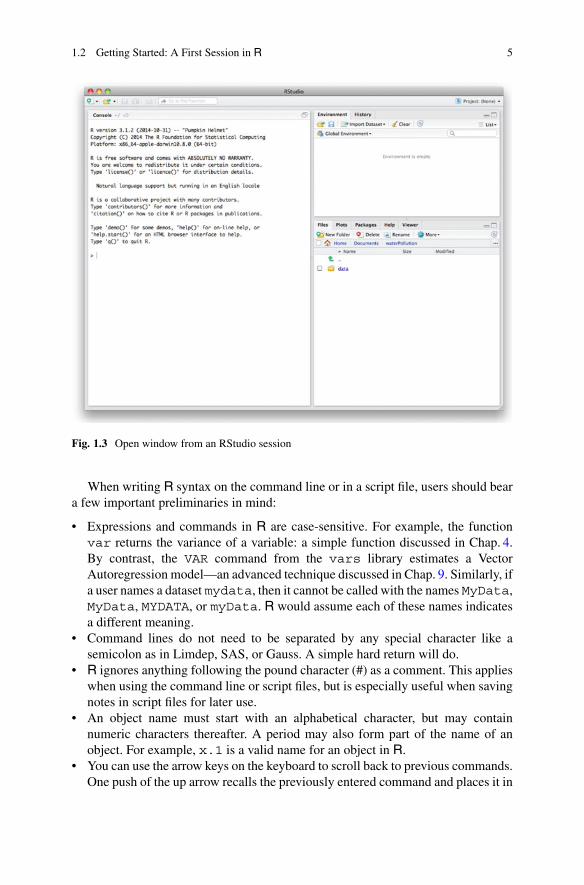
Once you have installed R, there will be an icon either under the WindowsStart menu (with an option of placing a shortcut on the Desktop) or in the MacApplications folder (with an option of keeping an icon in the workspace Dock).Clicking or double-clicking the icon will start R. Figure 1.2 shows the windowassociated with the Mac version of the software. You will notice that R does havea few push-button options at the top of the window. Within Mac, the menu bar atthe top of the workspace will also feature a few pull-down menus. In Windows,pull down menus also will be presented within the R window. With only a handfulof menus and buttons, however, commands in R are entered primarily through usercode. Users desiring the fallback option of having more menus and buttons availablemay wish to install RStudio or a similar program that adds a point-and-click frontend to R, but a knowledge of the syntax is essential. Figure 1.3 shows the windowassociated with the Mac version of RStudio.2
Users can submit their code either through script files (the recommended choice,described in Sect. 1.3) or on the command line displayed at the bottom of the Rconsole. In Fig. 1.2, the prompt looks like this:
>
1The names of these files change as new versions of R are released. As of this printing,the respective files are R-3.1.2-snowleopard.pkg or R-3.1.2-mavericks.pkg forvarious versions of Mac OS X and R-3.1.2-win.exe for Windows. Linux users will find iteasier to install from a terminal. Terminal code is available by following the Download R forLinux link on the CRAN page, then choosing a Linux distribution on the next page, and using theterminal code listed on the resulting page. At the time of printing, Debian, various forms of RedHat, OpenSUSE, and Ubuntu are all supported.2RStudio is available at http://www.rstudio.com.

4 1 Obtaining R and Downloading Packages
Fig. 1.2 R Console for a new session
Whenever typing code directly into the command prompt, if a user types a singlecommand that spans multiple lines, then the command prompt turns into a plus sign(+) to indicate that the command is not complete. The plus sign does not indicateany problem or error, but just reminds the user that the previous command is notyet complete. The cursor automatically places itself there so the user can entercommands.
In the electronic edition of this book, input syntax and output printouts from Rwill be color coded to help distinguish what the user should type in a script file fromwhat results to expect. Input code will be written in blue teletype font.R output will be written in black teletype font. Error messages that Rreturns will be written in red teletype font. These colors correspond tothe color coding R uses for input and output text. While the colors may not bevisible in the print edition, the book’s text also will distinguish inputs from outputs.Additionally, names of variables will be written in bold. Conceptual keywords fromstatistics and programming, as well as emphasized text, will be written in italics.Finally, when the meaning of a command is not readily apparent, identifying initialswill be underlined and bolded in the text. For instance, the lm command stands forlinear model.
1.2 Getting Started: A First Session in R 5
Fig. 1.3 Open window from an RStudio session
When writing R syntax on the command line or in a script file, users should beara few important preliminaries in mind:
• Expressions and commands in R are case-sensitive. For example, the functionvar returns the variance of a variable: a simple function discussed in Chap. 4.By contrast, the VAR command from the vars library estimates a VectorAutoregression model—an advanced technique discussed in Chap. 9. Similarly, ifa user names a dataset mydata, then it cannot be called with the names MyData,MyData, MYDATA, or myData. R would assume each of these names indicatesa different meaning.
• Command lines do not need to be separated by any special character like asemicolon as in Limdep, SAS, or Gauss. A simple hard return will do.
• R ignores anything following the pound character (#) as a comment. This applieswhen using the command line or script files, but is especially useful when savingnotes in script files for later use.
• An object name must start with an alphabetical character, but may containnumeric characters thereafter. A period may also form part of the name of anobject. For example, x.1 is a valid name for an object in R.
• You can use the arrow keys on the keyboard to scroll back to previous commands.One push of the up arrow recalls the previously entered command and places it in

6 1 Obtaining R and Downloading Packages
the command line. Each additional push of the arrow moves to a command priorto the one listed in the command line, while the down arrow calls the commandfollowing the one listed in the command line.
Aside from this handful of important rules, the command prompt in R tendsto behave in an intuitive way, returning responses to input commands that couldbe easily guessed. For instance, at its most basic level R functions as a high-endcalculator. Some of the key arithmetic commands are: addition (+), subtraction(-), multiplication (*), division (/), exponentiation (^ ), the modulo function (%%),and integer division (%/%). Parentheses ( ) specify the order of operations. Forexample, if we type the following input:
(3+5/78)^3*7
Then R prints the following output:
[1] 201.3761
As another example, we could ask R what the remainder is when dividing 89 by 13using the modulo function:
89%%13
R then provides the following answer:
[1] 11
If we wanted R to perform integer division, we could type:
89%/%13
Our output answer to this is:
[1] 6
The options command allows the user to tweak attributes of the output. Forexample, the digits argument offers the option to adjust how many digits aredisplayed. This is useful, for instance, when considering how precisely you wish topresent results on a table. Other useful built-in functions from algebra and trigonom-etry include: sin(x), cos(x), tan(x), exp(x), log(x), sqrt(x), and pi.To apply a few of these functions, first we can expand the number of digits printedout, and then ask for the value of the constant � :
options(digits=16)pi
R accordingly prints out the value of � to 16 digits:
[1] 3.141592653589793
We also may use commands such as pi to insert the value of such a constant intoa function. For example, if we wanted to compute the sine of a �
2radians (or 90ı)
angle, we could type:
sin(pi/2)
R correctly prints that sin. �2/ D 1:
[1] 1

1.3 Saving Input and Output 7
1.3 Saving Input and Output
When analyzing data or programming in R, a user will never get into serious troubleprovided he or she follows two basic rules:
1. Always leave the original datafiles intact. Any revised version of data should bewritten into a new file. If you are working with a particularly large and unwieldydataset, then write a short program that winnows-down to what you need, savethe cleaned file separately, and then write code that works with the new file.
2. Write all input code in a script that is saved. Users should usually avoid writingcode directly into the console. This includes code for cleaning, recoding, andreshaping data as well as for conducting analysis or developing new programs.
If these two rules are followed, then the user can always recover his or her work up tothe point of some error or omission. So even if, in data management, some essentialinformation is dropped or lost, or even if a journal reviewer names a predictor thata model should add, the user can always retrace his or her steps. By calling theoriginal dataset with the saved program, the user can make minor tweaks to thecode to incorporate a new feature of analysis or recover some lost information. Bycontrast, if the original data are overwritten or the input code is not saved, then theuser likely will have to restart the whole project from the beginning, which is a wasteof time.
A script file in R is simply plain text, usually saved with the suffix .R. To createa new script file in R, simply choose File!New Document in the drop down menuto open the document. Alternatively, the console window shown in Fig. 1.2 showsan icon that looks like a blank page at the top of the screen (second icon from theright). Clicking on this will also create a new R script file. Once open, the normalSave and Save As commands from the File menu apply. To open an existing R script,choose File!Open Document in the drop down menu, or click the icon at the topof the screen that looks like a page with writing on it (third icon from the right inFig. 1.2). When working with a script file, any code within the file can be executedin the console by simply highlighting the code of interest, and typing the keyboardshortcut Ctrl+R in Windows or Cmd+Return in Mac. Besides the default scriptfile editor, more sophisticated text editors such as Emacs and RWinEdt also areavailable.
The product of any R session is saved in the working directory. The workingdirectory is the default file path for all files the user wants to read in or write outto. The command getwd (meaning get working directory) will print R’s currentworking directory, while setwd (set working directory) allows you to change theworking directory as desired. Within a Windows machine the syntax for checking,and then setting, the working directory would look like this:
getwd()setwd("C:/temp/")

8 1 Obtaining R and Downloading Packages
This now writes any output files, be they data sets, figures, or printed output to thefolder temp in the C: drive. Observe that R expects forward slashes to designatesubdirectories, which contrasts from Windows’s typical use of backslashes. Hence,specifying C:/temp/ as the working directory points to C:\temp\ in normalWindows syntax. Meanwhile for Mac or Unix, setting a working directory would besimilar, and the path directory is printed exactly as these operating systems designatethem with forward slashes:
setwd("/Volumes/flashdisk/temp")
Note that setwd can be called multiple times in a session, as needed. Also,specifying the full path for any file overrides the working directory.
To save output from your session in R, try the sink command. As a generalcomputing term, a sink is an output point for a program where data or results arewritten out. In R, this term accordingly refers to a file that records all of our printedoutput. To save your session’s ouput to the file Rintro.txt within the workingdirectory type:
sink("Rintro.txt")
Alternatively, if we wanted to override the working directory, in Windows forinstance, we could have instead typed:
sink("C:/myproject/code/Rintro.txt")
Now that we have created an output file, any output that normally would print tothe console will instead print to the file Rintro.txt. (For this reason, in a firstrun of new code, it is usually advisable to allow output to print to the screen and thenrerun the code later to print to a file.) The print command is useful for creatingoutput that can be easily followed. For instance, the command:
print("The mean of variable x is...")
will print the following in the file Rintro.txt:
[1] "The mean of variable x is..."
Another useful printing command is the cat command (short for catenate, toconnect things together), which lets you mix objects in R with text. As a preview ofsimulation tools described in Chap. 11, let us create a variable named x by means ofsimulation:
x <- rnorm(1000)
By way of explanation: this syntax draws randomly 1000 times from a standardnormal distribution and assigns the values to the vector x. Observe the arrow (<-),formed with a less than sign and a hyphen, which is R’s assignment operator. Anytime we assign something with the arrow (<-) the name on the left (x in thiscase) allows us to recall the result of the operation on the right (rnorm(1000)

1.4 Work Session Management 9
in this case).3 Now we can print the mean of these 1000 draws (which should beclose to 0 in this case) to our output file as follows:
cat("The mean of variable x is...", mean(x), "\n")
With this syntax, objects from R can be embedded into the statement you print. Thecharacter \n puts in a carriage return. You also can print any statistical output usingthe either print or cat commands. Remember, your output does not go to the logfile unless you use one of the print commands. Another option is to simply copy andpaste results from the R console window into Word or a text editor. To turn off thesink command, simply type:
sink()
1.4 Work Session Management
A key feature of R is that it is an object-oriented programming language. Variables,data frames, models, and outputs are all stored in memory as objects, or identified(and named) locations in memory with defined features. R stores in workingmemory any object you create using the name you define whenever you load datainto memory or estimate a model. To list the objects you have created in a sessionuse either of the following commands:
objects()ls()
To remove all the objects in R type:
rm(list=ls(all=TRUE))
As a rule, it is a good idea to use the rm command at the start of any new program.If the previous user saved his or her workspace, then they may have used objectssharing the same name as yours, which can create confusion.
To quit R either close the console window or type:
q()
At this point, R will ask if you wish to save the workspace image. Generally, it isadvisable not to do this, as starting with a clean slate in each session is more likelyto prevent programming errors or confusion on the versions of objects loaded inmemory.
Finally, in many R sessions, we will need to load packages, or batches ofcode and data offering additional functionality not written in R’s base code.Throughout this book we will load several packages, particularly in Chap. 8, where
3The arrow (<-) is the traditional assignment operator, though a single equals sign (=) also canserve for assignments.
10 1 Obtaining R and Downloading Packages
our focus will be on example packages written by prominent Political Scientists toimplement cutting-edge methods. The necessary commands to load packages areinstall.packages, a command that automatically downloads and installs apackage on a user’s copy of R, and library, a command that loads the packagein a given session. Suppose we wanted to install the package MCMCpack. Thispackage provides tools for Bayesian modeling that we will use in Chap. 8. The formof the syntax for these commands is:
install.packages("MCMCpack")library(MCMCpack)
Package installation is case and spelling sensitive. R will likely prompt you at thispoint to choose one of the CRAN mirrors from which to download this package: Forfaster downloading, users typically choose the mirror that is most geographicallyproximate. The install.packages command only needs to be run once per Rinstallation for a particular package to be available on a machine. The librarycommand needs to be run for every session that a user wishes to use the package.Hence, in the next session that we want to use MCMCpack, we need only type:library(MCMCpack).
1.5 Resources
Given the wide array of base functions that are available in R, much less the evenwider array of functionality created by R packages, a book such as this cannotpossibly address everything R is capable of doing. This book should serve as aresource introducing how a researcher can use R as a basic statistics program andoffer some general pointers about the usage of packages and programming features.As questions emerge about topics not covered in this space, there are several otherresources that may be of use:
• Within R, the Help pull down menu (also available by typing help.start()in the console) offers several manuals of use, including an “Introduction to R”and “Writing R Extensions.” This also opens an HTML-based search engine ofthe help files.
• UCLA’s Institute for Digital Research and Education offers several nice tutorials(http://www.ats.ucla.edu/stat/r/). The CRAN website also includes a variety ofonline manuals (http://www.cran.r-project.org/other-docs.html).
• Some nice interactive tutorials include swirl, which is a package you install inyour own copy of R (more information: http://www.swirlstats.com/), and Try R,which is completed online (http://tryr.codeschool.com/).
• Within the R console, the commands ?, help(), and help.search() allserve to find documentation. For instance, ?lm would find the documenta-tion for the linear model command. Alternatively, help.search("linearmodel") would search the documentation for a phrase.

1.6 Practice Problems 11
• To search the internet for information, Rseek (http://www.rseek.org/, powered byGoogle) is a worthwhile search engine that searches only over websites focusedon R.
• Finally, Twitter users reference R through the hashtag #rstats.
At this point, users should now have R installed on their machine, hold a basicsense of how commands are entered and output is generated, and recognize whereto find the vast resources available for R users. In the next six chapters, we will seehow R can be used to fill the role of a statistical analysis or econometrics softwareprogram.
1.6 Practice Problems
Each chapter will end with a few practice problems. If you have tested all of thecode from the in-chapter examples, you should be able to complete these on yourown. If you have not done so already, go ahead and install R on your machine forfree and try the in-chapter code. Then try the following questions.
1. Compute the following in R:
(a) �7 � 23
(b) 882C1
(c) cos �
(d)p
81
(e) ln e4
2. What does the command cor do? Find documentation about it and describe whatthe function does.
3. What does the command runif do? Find documentation about it and describewhat the function does.
4. Create a vector named x that consists of 1000 draws from a standard normaldistribution, using code just like you see in Sect. 1.3. Create a second vectornamed y in the same way. Compute the correlation coefficient between the twovectors. What result do you get, and why do you get this result?
5. Get a feel for how to decide when add-on packages might be useful for you.Log in to http://www.rseek.org and look up what the stringr package does.What kinds of functionality does this package give you? When might you wantto use it?

Chapter 2Loading and Manipulating Data
We now turn to using R to conduct data analysis. Our first basic steps are simplyto load data into R and to clean the data to suit our purposes. Data cleaning andrecoding are an often tedious task of data analysis, but nevertheless are essentialbecause miscoded data will yield erroneous results when a model is estimated usingthem. (In other words, garbage in, garbage out.) In this chapter, we will load varioustypes of data using differing commands, view our data to understand their features,practice recoding data in order to clean them as we need to, merge data sets, andreshape data sets.
Our working example in this chapter will be a subset of Poe et al.’s (1999)Political Terror Scale data on human rights, which is an update of the data in Poeand Tate (1994). Whereas their complete data cover 1976–1993, we focus solely onthe year 1993. The eight variables this dataset contains are:
country: A character variable listing the country by name.democ: The country’s score on the Polity III democracy scale. Scores range from 0
(least democratic) to 10 (most democratic).sdnew: The U.S. State Department scale of political terror. Scores range from
1 (low state terrorism, fewest violations of personal integrity) to 5 (highestviolations of personal integrity).
military: A dummy variable coded 1 for a military regime, 0 otherwise.gnpcats: Level of per capita GNP in five categories: 1 = under $1000, 2 = $1000–
$1999, 3 = $2000–$2999, 4 = $3000–$3999, 5 = over $4000.lpop: Logarithm of national population.civ_war: A dummy variable coded 1 if involved in a civil war, 0 otherwise.int_war: A dummy variable coded 1 if involved in an international war, 0 otherwise.
Electronic supplementary material: The online version of this chapter(doi: 10.1007/978-3-319-23446-5_2) contains supplementary material, which is available toauthorized users.
© Springer International Publishing Switzerland 2015J.E. Monogan III, Political Analysis Using R, Use R!,DOI 10.1007/978-3-319-23446-5_2
13

14 2 Loading and Manipulating Data
2.1 Reading in Data
Getting data into R is quite easy. There are three primary ways to import data:Inputting the data manually (perhaps written in a script file), reading data froma text-formatted file, and importing data from another program. Since it is a bitless common in Political Science, inputting data manually is illustrated in theexamples of Chap. 10, in the context of creating vectors, matrices, and data frames.In this section, we focus on importing data from saved files.
First, we consider how to read in a delimited text file with the read.tablecommand. R will read in a variety of delimited files. (For all the options associatedwith this command type ?read.table in R.) In text-based data, typically eachline represents a unique observation and some designated delimiter separates eachvariable on the line. The default for read.table is a space-delimited file whereinany blank space designates differing variables. Since our Poe et al. data file,named hmnrghts.txt, is space-separated, we can read our file into R using thefollowing line of code. This data file is available from the Dataverse named on pagevii or the chapter content link on page 13. You may need to use setwd commandintroduced in Chap. 1 to point R to the folder where you have saved the data. Afterthis, run the following code:
hmnrghts<-read.table("hmnrghts.txt",header=TRUE, na="NA")
Note: As was mentioned in the previous chapter, R allows the user to split a singlecommand across multiple lines, which we have done here. Throughout this book,commands that span multiple lines will be distinguished with hanging indentation.Moving to the code itself, observe a few features: One, as was noted in the previouschapter, the left arrow symbol (<-) assigns our input file to an object. Hence,hmnrghts is the name we allocated to our data file, but we could have called itany number of things. Second, the first argument of the read.table commandcalls the name of the text file hmnrghts.txt. We could have preceded thisargument with the file= option—and we would have needed to do so if we hadnot listed this as the first argument—but R recognizes that the file itself is normallythe first argument this command takes. Third, we specified header=TRUE, whichconveys that the first row of our text file lists the names of our variables. It isessential that this argument be correctly identified, or else variable names may beerroneously assigned as data or data as variable names.1 Finally, within the text file,the characters NA are written whenever an observation of a variable is missing. Theoption na="NA" conveys to R that this is the data set’s symbol for a missing value.(Other common symbols of missingness are a period (.) or the number -9999.)
The command read.table also has other important options. If your text fileuses a delimiter other than a space, then this can be conveyed to R using the sepoption. For instance, including sep="\t" in the previous command would have
1A closer look at the file itself will show that our header line of variable names actually has onefewer element than each line of data. When this is the case, R assumes that the first item on eachline is an observation index. Since that is true in this case, our data are read correctly.

2.1 Reading in Data 15
allowed us to read in a tab-separated text file, while sep=","would have allowed acomma-separated file. The commands read.csv and read.delim are alternateversions of read.table that merely have differing default values. (Particularly,read.csv is geared to read comma-separated values files and read.delimis geared to read tab-delimited files, though a few other defaults also change.)Another important option for these commands is quote. The defaults vary acrossthese commands for which characters designate string-based variables that usealphabetic text as values, such as the name of the observation (e.g., country, state,candidate). The read.table command, by default, uses either single or doublequotation marks around the entry in the text file. This would be a problem ifdouble quotes were used to designate text, but apostrophes were in the text. Tocompensate, simply specify the option quote = "\"" to only allow doublequotes. (Notice the backslash to designate that the double-quote is an argument.)Alternatively, read.csv and read.delim both only allow double quotes bydefault, so specifying quote = "\"’" would allow either single or doublequotes, or quote = "\’"would switch to single quotes. Authors also can specifyother characters in this option, if need be.
Once you download a file, you have the option of specifying the full pathdirectory in the command to open the file. Suppose we had saved hmnrghts.txtinto the path directory C:/temp/, then we could load the file as follows:
hmnrghts <- read.table("C:/temp/hmnrghts.txt",header=TRUE, na="NA")
As was mentioned when we first loaded the file, another option would have been touse the setwd command to set the working directory, meaning we would not haveto list the entire file path in the call to read.table. (If we do this, all input andoutput files will go to this directory, unless we specify otherwise.) Finally, in anyGUI-based system (e.g., non-terminal), we could instead type:
hmnrghts<-read.table(file.choose(),header=TRUE,na="NA")
The file.choose() option will open a file browser allowing the user to locateand select the desired data file, which R will then assign to the named object inmemory (hmnrghts in this case). This browser option is useful in interactiveanalysis, but less useful for automated programs.
Another format of text-based data is a fixed width file. Files of this format do notuse a character to delimit variables within an observation. Instead, certain columnsof text are consistently dedicated to a variable. Thus, R needs to know whichcolumns define each variable to read in the data. The command for reading a fixedwidth file is read.fwf. As a quick illustration of how to load this kind of data, wewill load a different dataset—roll call votes from the 113th United States Senate, theterm running from 2013 to 2015.2 This dataset will be revisited in a practice problem
2These data were gathered by Jeff Lewis and Keith Poole. For more information, see http://www.voteview.com/senate113.htm.

16 2 Loading and Manipulating Data
in Chap. 8. To open these data, start by downloading the file sen113kh.ord fromthe Dataverse listed on page vii or the chapter content link on page 13. Then type:
senate.113<-read.fwf("sen113kh.ord",widths=c(3,5,2,2,8,3,1,1,11,rep(1,657)))
The first argument of read.fwf is the name of the file, which we draw froma URL. (The file extension is .ord, but the format is plain text. Try openingthe file in Notepad or TextEdit just to get a feel for the formatting.) The secondargument, widths, is essential. For each variable, we must enter the number ofcharacters allocated to that variable. In other words, the first variable has threecharacters, the second has five characters, and so on. This procedure should makeit clear that we must have a codebook for a fixed width file, or inputting the datais a hopeless endeavor. Notice that the last component in the widths argumentis rep(1,657). This means that our data set ends with 657 variables that areone character long. These are the 657 votes that the Senate cast during that term ofCongress, with each variable recording whether each senator voted yea, nay, present,or did not vote.
With any kind of data file, including fixed width, if the file itself does not havenames of the variables, we can add these in R. (Again, a good codebook is usefulhere.) The commands read.table, read.csv, and read.fwf all include anoption called col.names that allows the user to name every variable in the datasetwhen reading in the file. In the case of the Senate roll calls, though, it is easier forus to name the variables afterwards as follows:
colnames(senate.113)[1:9]<-c("congress","icpsr","state.code","cd","state.name","party","occupancy","attaining","name")
for(i in 1:657){colnames(senate.113)[i+9]<-paste("RC",i,sep="")}
In this case, we use the colnames command to set the names of the variables. Tothe left of the arrow, by specifying [1:9], we indicate that we are only naming thefirst nine variables. To the right of the arrow, we use one of the most fundamentalcommands in R: the combine command (c), which combines several elements intoa vector. In this case, our vector includes the names of the variables in text. On thesecond line, we proceed to name the 657 roll call votes RC1, RC2, . . . , RC657.To save typing we make this assignment using a for loop, which is described inmore detail in Chap. 11. Within the for loop, we use the paste command, whichsimply prints our text ("RC") and the index number i, separated by nothing (hencethe empty quotes at the end). Of course, by default, R assigns generic variable names(V1, V2, etc.), so a reader who is content to use generic names can skip this step,if preferred. (Bear in mind, though, that if we name the first nine variables like wedid, the first roll call vote would be named V10 without our applying a new name.)

2.1 Reading in Data 17
2.1.1 Reading Data from Other Programs
Turning back to our human rights example, you also can import data from manyother statistical programs. One of the most important libraries in R is the foreignpackage, which makes it very easy to bring in data from other statistical packages,such as SPSS, Stata, and Minitab.3 As an alternative to the text version of the humanrights data, we also could load a Stata-formatted data file, hmnrghts.dta.
Stata files generally have a file extension of dta, which is what the read.dtacommand refers to. (Similarly, read.spss will read an SPSS-formatted file withthe .sav file extension.) To open our data in Stata format, we need to download thefile hmnrghts.dta from the Dataverse linked on page vii or the chapter contentlinked on page 13. Once we save it to our hard drive, we can either set our workingdirectory, list the full file path, or use the file.choose() command to access ourdata . For example, if we downloaded the file, which is named hmnrghts.dta,into our C:\temp\ folder, we could open it by typing:
library(foreign)setwd("C:/temp/")hmnrghts.2 <- read.dta("hmnrghts.dta")
Any data in Stata format that you select will be converted to R format. One word ofwarning, by default if there are value labels on Stata-formatted data, R will importthe labels as a string-formatted variable. If this is an issue for you, try importingthe data without value labels to save the variables using the numeric codes. See thebeginning of Chap. 7 for an example of the convert.factors=FALSE option.(One option for data sets that are not excessively large is to load two copies of aStata dataset—one with the labels as text to serve as a codebook and another withnumerical codes for analysis.) It is always good to see exactly how the data areformatted by inspecting the spreadsheet after importing with the tools described inSect. 2.2.
2.1.2 Data Frames in R
R distinguishes between vectors, lists, data frames, and matrices. Each of theseis an object of a different class in R. Vectors are indexed by length, and matricesare indexed by rows and columns. Lists are not pervasive to basic analyses, butare handy for complex storage and are often thought of as generic vectors whereeach element can be any class of object. (For example, a list could be a vector of
3The foreign package is so commonly used that it now downloads with any new R installation.In the unlikely event, though, that the package will not load with the library command,simply type install.packages("foreign") in the command prompt to download it.Alternatively, for users wishing to import data from Excel, two options are present: One is tosave the Excel file in comma-separated values format and then use the read.csv command. Theother is to install the XLConnect library and use the readWorksheetFromFile command.

18 2 Loading and Manipulating Data
model results, or a mix of data frames and maps.) A data frame is a matrix thatR designates as a data set. With a data frame, the columns of the matrix can bereferred to as variables. After reading in a data set, R will treat your data as a dataframe, which means that you can refer to any variable within a data frame by adding$VARIABLENAME to the name of the data frame.4 For example, in our human rightsdata we can print out the variable country in order to see which countries are inthe dataset:
hmnrghts$country
Another option for calling variables, though an inadvisable one, is to use theattach command. R allows the user to load multiple data sets at once (in contrastto some of the commercially available data analysis programs). The attachcommand places one dataset at the forefront and allows the user to call directly thenames of the variables without referring the name of the data frame. For example:
attach(hmnrghts)country
With this code, R would recognize country in isolation as part of the attacheddataset and print it just as in the prior example. The problem with this approach isthat R may store objects in memory with the same name as some of the variables inthe dataset. In fact, when recoding data the user should always refer to the data frameby name, otherwise R confusingly will create a copy of the variable in memory thatis distinct from the copy in the data frame. For this reason, I generally recommendagainst attaching data. If, for some circumstance, a user feels attaching a data frameis unavoidable, then the user can conduct what needs to be done with the attacheddata and then use the detach command as soon as possible. This command worksas would be expected, removing the designation of a working data frame and nolonger allowing the user to call variables in isolation:
detach(hmnrghts)
2.1.3 Writing Out Data
To export data you are using in R to a text file, use the functions write.table orwrite.csv. Within the foreign library, write.dta allows the user to writeout a Stata-formatted file. As a simple example, we can generate a matrix with fourobservations and six variables, counting from 1 to 24. Then we can write this to acomma-separated values file, a space-delimited text file, and a Stata file:
x <- matrix(1:24, nrow=4)write.csv(x, file="sample.csv")write.table(x, file="sample.txt")write.dta(as.data.frame(x), file="sample.dta")
4More technically, data frames are objects of the S3 class. For all S3 objects, attributes of theobject (such as variables) can be called with the dollar sign ($).

2.2 Viewing Attributes of the Data 19
Note that the command as.data.frame converts matrices to data frames, adistinction described in the prior section. The command write.dta expects theobject to be of the data.frame class. Making this conversion is unnecessary ifthe object is already formatted as data, rather than a matrix. To check your effort insaving the files, try removing x from memory with the command rm(x) and thenrestoring the data from one of the saved files.
To keep up with where the saved data files are going, the files we write out willbe saved in our working directory. To get the working directory (that is, have Rtell us what it is), simply type: getwd(). To change the working directory whereoutput files will be written, we can set the working directory, using the same setwdcommand that we considered when opening files earlier. All subsequently saved fileswill be output into the specified directory, unless R is explicitly told otherwise.
2.2 Viewing Attributes of the Data
Once data are input into R, the first task should be to inspect the data and make surethey have loaded properly. With a relatively small dataset, we can simply print thewhole data frame to the screen:
hmnrghts
Printing the entire dataset, of course, is not recommended or useful with largedatasets. Another option is to look at the names of the variables and the first fewlines of data to see if the data are structured correctly through a few observations.This is done with the head command:
head(hmnrghts)
For a quick list of the names of the variables in our dataset (which can also be usefulif exact spelling or capitalization of variable names is forgotten) type:
names(hmnrghts)
A route to getting a comprehensive look at the data is to use the fix command:
fix(hmnrghts)
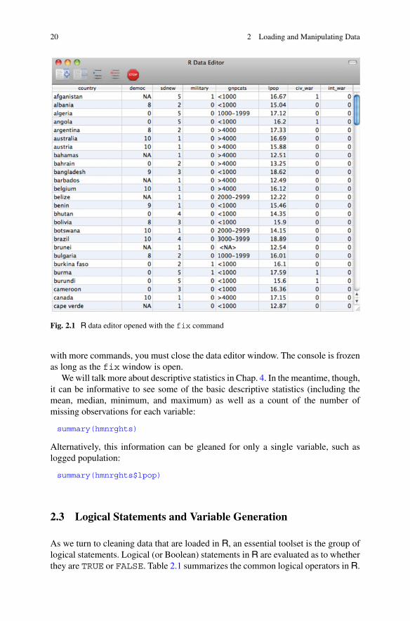
This presents the data in a spreadsheet allowing for a quick view of observations orvariables of interest, as well as a chance to see that the data matrix loaded properly.An example of this data editor window that fix opens is presented in Fig. 2.1. Theuser has the option of editing data within the spreadsheet window that fix creates,though unless the revised data are written to a new file, there will be no permanentrecord of these changes.5 Also, it is key to note that before continuing an R session
5The View command is similar to fix, but does not allow editing of observations. If you prefer toonly be able to see the data without editing values (perhaps even by accidentally leaning on yourkeyboard), then View might be preferable.
20 2 Loading and Manipulating Data
Fig. 2.1 R data editor opened with the fix command
with more commands, you must close the data editor window. The console is frozenas long as the fix window is open.
We will talk more about descriptive statistics in Chap. 4. In the meantime, though,it can be informative to see some of the basic descriptive statistics (including themean, median, minimum, and maximum) as well as a count of the number ofmissing observations for each variable:
summary(hmnrghts)
Alternatively, this information can be gleaned for only a single variable, such aslogged population:
summary(hmnrghts$lpop)
2.3 Logical Statements and Variable Generation
As we turn to cleaning data that are loaded in R, an essential toolset is the group oflogical statements. Logical (or Boolean) statements in R are evaluated as to whetherthey are TRUE or FALSE. Table 2.1 summarizes the common logical operators in R.

2.3 Logical Statements and Variable Generation 21
Table 2.1 Logical operators in ROperator Means< Less than<= Less than or equal to> Greater than>= Greater than or equal to== Equal to!= Not equal to& And| Or
Note that the Boolean statement “is equal to” is designated by two equals signs (==),whereas a single equals sign (=) instead serves as an assignment operator.
To apply some of these Boolean operators from Table 2.1 in practice, suppose, forexample, we wanted to know which countries were in a civil war and had an aboveaverage democracy score in 1993. We could generate a new variable in our workingdataset, which I will call dem.civ (though the user may choose the name). Thenwe can view a table of our new variable and list all of the countries that fit thesecriteria:
hmnrghts$dem.civ <- as.numeric(hmnrghts$civ_war==1 &hmnrghts$democ>5.3)
table(hmnrghts$dem.civ)hmnrghts$country[hmnrghts$dem.civ==1]
On the first line, hmnrghts$dem.civ defines our new variable within the humanrights dataset.6 On the right, we have a two-part Boolean statement: The first askswhether the country is in a civil war, and the second asks if the country’s democracyscore is higher than the average of 5.3. The ampersand (&) requires that bothstatements must simultaneously be true for the whole statement to be true. All ofthis is embedded within the as.numeric command, which encodes our Booleanoutput as a numeric variable. Specifically, all values of TRUE are set to 1 andFALSE values are set to 0. Such a coding is usually more convenient for modelingpurposes. The next line gives us a table of the relative frequencies of 0s and 1s.It turns out that only four countries had above-average democracy levels and wereinvolved in a civil war in 1993. To see which countries, the last line asks R to printthe names of countries, but the square braces following the vector indicate whichobservations to print: Only those scoring 1 on this new variable.7
6Note, though, that any new variables we create, observations we drop, or variables we recode onlychange the data in working memory. Hence, our original data file on disk remains unchanged andtherefore safe for recovery. Again, we must use one of the commands from Sect. 2.1.3 if we wantto save a second copy of the data including all of our changes.7The output prints the four country names, and four values of NA. This means in four cases, one ofthe two component statements was TRUE but the other statement could not be evaluated becausethe variable was missing.

22 2 Loading and Manipulating Data
Another sort of logical statement in R that can be useful is the is statement.These statements ask whether an observation or object meets some criterion. Forexample, is.na is a special case that asks whether an observation is missing or not.Alternatively, statements such as is.matrix or is.data.frame ask whetheran object is of a certain class. Consider three examples:
table(is.na(hmnrghts$democ))is.matrix(hmnrghts)is.data.frame(hmnrghts)
The first statement asks for each observation whether the value of democracy ismissing. The table command then aggregates this and informs us that 31 observa-tions are missing. The next two statements ask whether our dataset hmnrghtsis saved as a matrix, then as a data frame. The is.matrix statement returnsFALSE, indicating that matrix-based commands will not work on our data, and theis.data.frame statement returns TRUE, which indicates that it is stored as adata frame. With a sense of logical statements in R, we can now apply these to thetask of cleaning data.
2.4 Cleaning Data
One of the first tasks of data cleaning is deciding how to deal with missing data. Rdesignates missing values with NA. It translates missing values from other statisticspackages into the NA missing format. However a scholar deals with missing data,it is important to be mindful of the relative proportion of unobserved values in thedata and what information may be lost. One (somewhat crude) option to deal withmissingness would be to prune the dataset through listwise deletion, or removingevery observation for which a single variable is not recorded. To create a new dataset that prunes in this way, type:
hmnrghts.trim <- na.omit(hmnrghts)
This diminishes the number of observations from 158 to 127, so a tangible amountof information has been lost.
Most modeling commands in R give users the option of estimating the modelover complete observations only, implementing listwise deletion on the fly. As awarning, listwise deletion is actually the default in the base commands for linearand generalized linear models, so data loss can fly under the radar if the user isnot careful. Users with a solid background on regression-based modeling are urgedto consider alternative methods for dealing with missing data that are superior tolistwise deletion. In particular, the mice and Amelia libraries implement theuseful technique of multiple imputation (for more information see King et al. 2001;Little and Rubin 1987; Rubin 1987).
If, for some reason, the user needs to redesignate missing values as havingsome numeric value, the is.na command can be useful. For example, if it werebeneficial to list missing values as �9999, then these could be coded as:
hmnrghts$democ[is.na(hmnrghts$democ)]<- -9999

2.4 Cleaning Data 23
In other words, all values of democracy for which the value is missing will takeon the value of �9999. Be careful, though, as R and all of its modeling commandswill now regard the formerly missing value as a valid observation and will insertthe misleading value of �9999 into any analysis. This sort of action should only betaken if it is required for data management, a special kind of model where strangevalues can be dummied-out, or the rare case where a missing observation actuallycan take on a meaningful value (e.g., a budget dataset where missing items representa $0 expenditure).
2.4.1 Subsetting Data
In many cases, it is convenient to subset our data. This may mean that we only wantobservations of a certain type, or it may mean we wish to winnow-down the numberof variables in the data frame, perhaps because the data include many variables thatare of no interest. If, in our human rights data, we only wanted to focus on countriesthat had a democracy score from 6–10, we could call this subset dem.rights andcreate it as follows:
dem.rights <- subset(hmnrghts, subset=democ>5)
This creates a 73 observation subset of our original data. Note that observationswith a missing (NA) value of democ will not be included in the subset. Missingobservations also would be excluded if we made a greater than or equal tostatement.8
As an example of variable selection, if we wanted to focus only on democracyand wealth, we could keep only these two variables and an index for all observations:
dem.wealth<-subset(hmnrghts,select=c(country, democ, gnpcats))
An alternative means of selecting which variables we wish to keep is to use aminus sign after the select option and list only the columns we wish to drop. Forexample, if we wanted all variables except the two indicators of whether a countrywas at war, we could write:
no.war <- subset(hmnrghts,select=-c(civ_war,int_war))
Additionally, users have the option of calling both the subset and selectoptions if they wish to choose a subset of variables over a specific set ofobservations.
8This contrasts from programs like Stata, which treat missing values as positive infinity. In Stata,whether missing observations are included depends on the kind of Boolean statement being made.R is more consistent in that missing cases are always excluded.

24 2 Loading and Manipulating Data
2.4.2 Recoding Variables
A final aspect of data cleaning that often arises is the need to recode variables. Thismay emerge because the functional form of a model requires a transformation of avariable, such as a logarithm or square. Alternately, some of the values of the datamay be misleading and thereby need to be recoded as missing or another value. Yetanother possibility is that the variables from two datasets need to be coded on thesame scale: For instance, if an analyst fits a model with survey data and then makesforecasts using Census data, then the survey and Census variables need to be codedthe same way.
For mathematical transformations of variables, the syntax is straightforward andfollows the form of the example below. Suppose we want the actual population ofeach country instead of its logarithm:
hmnrghts$pop <- exp(hmnrghts$lpop)
Quite simply, we are applying the exponential function (exp) to a logged value torecover the original value. Yet any type of mathematical operator could be sub-stituted in for exp. A variable could be squared (ˆ2), logged (log()), havethe square root taken (sqrt()), etc. Addition, subtraction, multiplication, anddivision are also valid—either with a scalar of interest or with another variable.Suppose we wanted to create an ordinal variable coded 2 if a country was in both acivil war and an international war, 1 if it was involved in either, and 0 if it was notinvolved in any wars. We could create this by adding the civil war and internationalwar variables:
hmnrghts$war.ord<-hmnrghts$civ_war+hmnrghts$int_war
A quick table of our new variable, however, reveals that no nations had both kindsof conflict going in 1993.
Another common issue to address is when data are presented in an undesirableformat. Our variable gnpcats is actually coded as a text variable. However, wemay wish to recode this as a numeric ordinal variable. There are two means ofaccomplishing this. The first, though taking several lines of code, can be completedquickly with a fair amount of copy-and-paste:
hmnrghts$gnp.ord <- NAhmnrghts$gnp.ord[hmnrghts$gnpcats=="<1000"]<-1hmnrghts$gnp.ord[hmnrghts$gnpcats=="1000-1999"]<-2hmnrghts$gnp.ord[hmnrghts$gnpcats=="2000-2999"]<-3hmnrghts$gnp.ord[hmnrghts$gnpcats=="3000-3999"]<-4hmnrghts$gnp.ord[hmnrghts$gnpcats==">4000"]<-5
Here, a blank variable was created, and then the values of the new variable filled-incontingent on the values of the old using Boolean statements.
A second option for recoding the GNP data can be accomplished through JohnFox’s companion to applied regression (car) library. As a user-written library, wemust download and install it before the first use. The installation of a library isstraightforward. First, type:
install.packages("car")

2.4 Cleaning Data 25
Once the library is installed (again, a step which need not be repeated unless R isreinstalled), the following lines will generate our recoded per capita GNP measure:
library(car)hmnrghts$gnp.ord.2<-recode(hmnrghts$gnpcats,’"<1000"=1;
"1000-1999"=2;"2000-2999"=3;"3000-3999"=4;">4000"=5’)
Be careful that the recode command is delicate. Between the apostrophes, allof the reassignments from old values to new are defined separated by semicolons.A single space between the apostrophes will generate an error. Despite this,recode can save users substantial time on data cleaning. The basic syntax ofrecode, of course, could be used to create dummy variables, ordinal variables,or a variety of other recoded variables. So now two methods have created a newvariable, each coded 1 to 5, with 5 representing the highest per capita GNP.
Another standard type of recoding we might want to do is to create a dummyvariable that is coded as 1 if the observation meets certain conditions and 0otherwise. For example, suppose instead of having categories of GNP, we just wantto compare the highest category of GNP to all the others:
hmnrghts$gnp.dummy<-as.numeric(hmnrghts$gnpcats==">4000")
As with our earlier example of finding democracies involved in a civil war, here weuse a logical statement and modify it with the as.numeric statement, which turnseach TRUE into a 1 and each FALSE into a 0.
Categorical variables in R can be given a special designation as factors. If youdesignate a categorical variable as a factor, R will treat it as such in statisticaloperation and create dummy variables for each level when it is used in a regression.If you import a variable with no numeric coding, R will automatically call thevariable a character vector, and convert the character vector into a factor in mostanalysis commands. If we prefer, though, we can designate that a variable is a factorahead of time and open up a variety of useful commands. For example, we candesignate country as a factor:
hmnrghts$country <- as.factor(hmnrghts$country)levels(hmnrghts$country)
Notice that R allows the user to put the same quantity (in this case, the variablecountry) on both sides of an assignment operator. This recursive assignment takesthe old values of a quantity, makes the right-hand side change, and then replaces thenew values into the same place in memory. The levels command reveals to us thedifferent recorded values of the factor.
To change which level is the first level (e.g., to change which category R willuse as the reference category in a regression) use the relevel command. Thefollowing code sets “united states” as the reference category for country:
hmnrghts$country<-relevel(hmnrghts$country,"united states")levels(hmnrghts$country)
Now when we view the levels of the factor, “united states” is listed as the first level,and the first level is always our reference group.
26 2 Loading and Manipulating Data
2.5 Merging and Reshaping Data
Two final tasks that are common to data management are merging data sets andreshaping panel data. As we consider examples of these two tasks, let us consider anupdate of Poe et al.’s (1999) data: Specifically, Gibney et al. (2013) have continuedto code data for the Political Terror Scale. We will use the 1994 and 1995 waves ofthe updated data. The variables in these waves are:
Country: A character variable listing the country by name.COWAlpha: Three-character country abbreviation from the Correlates of War
dataset.COW: Numeric country identification variable from the Correlates of War dataset.WorldBank: Three-character country abbreviation used by the World Bank.Amnesty.1994/Amnesty.1995: Amnesty International’s scale of political terror.
Scores range from 1 (low state terrorism, fewest violations of personal integrity)to 5 (highest violations of personal integrity).
StateDept.1994/StateDept.1995: The U.S. State Department scale of politicalterror. Scores range from 1 (low state terrorism, fewest violations of personalintegrity) to 5 (highest violations of personal integrity).
For the last two variables, the name of the variable depends on which wave of datais being studied, with the suffix indicating the year. Notice that these data have fouridentification variables: This is designed explicitly to make these data easier forresearchers to use. Each index makes it easy for a researcher to link these politicalterror measures to information provided by either the World Bank or the Correlatesof War dataset. This should show how ubiquitous the act of merging data is toPolitical Science research.
To this end, let us practice merging data. In general, merging data is usefulwhen the analyst has two separate data frames that contain information about thesame observations. For example, if a Political Scientist had one data frame witheconomic data by country and a second data frame containing election returns bycountry, the scholar might want to merge the two data sets to link economic andpolitical factors within each country. In our case, suppose we simply wanted tolink each country’s political terror score from 1994 to its political terror score from1995. First, download the data sets pts1994.csv and pts1995.csv from theDataverse on page vii or the chapter content link on page 13. As before, you mayneed to use setwd to point R to the folder where you have saved the data. Afterthis, run the following code to load the relevant data:
hmnrghts.94<-read.csv("pts1994.csv")hmnrghts.95<-read.csv("pts1995.csv")
These data are comma separated, so read.csv is the best command in this case.If we wanted to take a look at the first few observations of our 1994 wave, we
could type head(hmnrghts.94). This will print the following:

2.5 Merging and Reshaping Data 27
Country COWAlpha COW WorldBank1 United States USA 2 USA2 Canada CAN 20 CAN3 Bahamas BHM 31 BHS4 Cuba CUB 40 CUB5 Haiti HAI 41 HTI6 Dominican Republic DOM 42 DOM
Amnesty.1994 StateDept.19941 1 NA2 1 13 1 24 3 35 5 46 2 2
Similarly, head(hmnrghts.95) will print the first few observations of our 1995wave:
Country COWAlpha COW WorldBank1 United States USA 2 USA2 Canada CAN 20 CAN3 Bahamas BHM 31 BHS4 Cuba CUB 40 CUB5 Haiti HAI 41 HTI6 Dominican Republic DOM 42 DOM
Amnesty.1995 StateDept.19951 1 NA2 NA 13 1 14 4 35 2 36 2 2
As we can see from our look at the top of each data frame, the data are orderedsimilarly in each case, and our four index variables have the same name in eachrespective data set. We only need one index to merge our data, and the other threeare redundant. For this reason, we can drop three of the index variables from the1995 data:hmnrghts.95<-subset(hmnrghts.95,
select=c(COW,Amnesty.1995,StateDept.1995))
We opted to delete the three text indices in order to merge on a numeric index.This choice is arbitrary, however, because R has no problem merging on a charactervariable either. (Try replicating this exercise by merging on COWAlpha, forexample.)

28 2 Loading and Manipulating Data
To combine our 1994 and 1995 data, we now turn to the merge command.9
We type:
hmnrghts.wide<-merge(x=hmnrghts.94,y=hmnrghts.95,by=c("COW"))
Within this command, the option x refers to one dataset, while y is the other. Nextto the by option, we name an identification variable that uniquely identifies eachobservation. The by command actually allows users to name multiple variablesif several are needed to uniquely identify each observation: For example, if aresearcher was merging data where the unit of analysis was a country-year, a countryvariable and a year variable might be essential to identify each row uniquely. In sucha case the syntax might read, by=c("COW","year"). As yet another option,if the two datasets had the same index, but the variables were named differently,R allows syntax such as, by.x=c("COW"), by.y=c("cowCode"), whichconveys that the differently named index variables are the name.
Once we have merged our data, we can preview the finished product by typinghead(hmnrghts.wide). This prints:
COW Country COWAlpha WorldBank Amnesty.19941 2 United States USA USA 12 20 Canada CAN CAN 13 31 Bahamas BHM BHS 14 40 Cuba CUB CUB 35 41 Haiti HAI HTI 56 42 Dominican Republic DOM DOM 2
StateDept.1994 Amnesty.1995 StateDept.19951 NA 1 NA2 1 NA 13 2 1 14 3 4 35 4 2 36 2 2 2
As we can see, the 1994 and 1995 scores for Amnesty and StateDept are recordedin one place for each country. Hence, our merge was successful. By default, Rexcludes any observation from either dataset that does not have a linked observation(e.g., equivalent value) from the other data set. So if you use the defaults and the newdataset includes the same number of rows as the two old datasets, then all observationswere linked and included. For instance, we could type:
dim(hmnrghts.94); dim(hmnrghts.95); dim(hmnrghts.wide)
This would quickly tell us that we have 179 observations in both of the inputs, as wellas the output dataset, showing we did not lose any observations. Other options withinmerge are all.x, all.y, and all, which allow you to specify whether to force
9Besides the merge, the dplyr package offers several data-joining commands that you also mayfind of use, depending on your needs.

2.5 Merging and Reshaping Data 29
the inclusion of all observations from the dataset x, the dataset y, and from eitherdataset, respectively. In this case, R would encode NA values for observations that didnot have a linked case in the other dataset.
As a final point of data management, sometimes we need to reshape our data. Inthe case of our merged data set, hmnrghts.wide, we have created a panel data set(e.g., a data set consisting of repeated observations of the same individuals) that is inwide format. Wide format means that each row in our data defines an individual ofstudy (a country) while our repeated observations are stored in separate variables (e.g.,Amnesty.1994 and Amnesty.1995 record Amnesty International scores for twoseparate years). In most models of panel data, we need our data to be in long format,or stacked format. Long format means that we need two index variables to identifyeach row, one for the individual (e.g., country) and one for time of observation (e.g.,year). Meanwhile, each variable (e.g., Amnesty) will only use one column. R allowsus to reshape our data from wide to long, or from long to wide. Hence, whatever theformat of our data, we can reshape it to our needs.
To reshape our political terror data from wide format to long, we use the reshapecommand:
hmnrghts.long<-reshape(hmnrghts.wide,varying=c("Amnesty.1994","StateDept.1994","Amnesty.1995","StateDept.1995"),timevar="year",idvar="COW",direction="long",sep=".")
Within the command, the first argument is the name of the data frame we wishto reshape. The varying term lists all of the variables that represent repeatedobservations over time. Tip: Be sure that repeated observations of the same variablehave the same prefix name (e.g., Amnesty or StateDept) and then the suffix(e.g., 1994 or 1995) consistently reports time. The timevar term allows us tospecify the name of our new time index, which we call year. The idvar termlists the variable that uniquely identifies individuals (countries, in our case). Withdirection we specify that we want to convert our data into long format. Lastly,the sep command offers R a cue of what character separates our prefixes and suffixesin the repeated observation variables: Since a period (.) separates these terms in eachof our Amnesty and StateDept variables, we denote that here.
A preview of the result can be seen by typing head(hmnrghts.long). Thisprints:
COW Country COWAlpha WorldBank year2.1994 2 United States USA USA 199420.1994 20 Canada CAN CAN 199431.1994 31 Bahamas BHM BHS 199440.1994 40 Cuba CUB CUB 199441.1994 41 Haiti HAI HTI 199442.1994 42 Dominican Republic DOM DOM 1994
Amnesty StateDept2.1994 1 NA20.1994 1 1

30 2 Loading and Manipulating Data
31.1994 1 240.1994 3 341.1994 5 442.1994 2 2
Notice that we now have only one variable for Amnesty and one forStateDept. We now have a new variable named year, so between COWand year, each row uniquely identifies each country-year. Since the dataare naturally sorted, the top of our data only show 1994 observations.Typing head(hmnrghts.long[hmnrghts.long$year==1995,]) showsus the first few 1995 observations:
COW Country COWAlpha WorldBank year2.1995 2 United States USA USA 199520.1995 20 Canada CAN CAN 199531.1995 31 Bahamas BHM BHS 199540.1995 40 Cuba CUB CUB 199541.1995 41 Haiti HAI HTI 199542.1995 42 Dominican Republic DOM DOM 1995
Amnesty StateDept2.1995 1 NA20.1995 NA 131.1995 1 140.1995 4 341.1995 2 342.1995 2 2
As we can see, all of the information is preserved, now in long (or stacked) format.As a final illustration, suppose we had started with a data set that was in long format
and wanted one in wide format. To try this, we will reshape hmnrghts.long andtry to recreate our original wide data set. To do this, we type:
hmnrghts.wide.2<-reshape(hmnrghts.long,v.names=c("Amnesty","StateDept"),timevar="year",idvar="COW",direction="wide",sep=".")
A few options have now changed: We now use the v.names command to indicatethe variables that include repeated observations. The timevar parameter now needsto be a variable within the dataset, just as idvar is, in order to separate individualsfrom repeated time points. Our direction term is now wide because we wantto convert these data into wide format. Lastly, the sep command specifies thecharacter that R will use to separate prefixes from suffixes in the final form. Bytyping head(hmnrghts.wide.2) into the console, you will now see that thisnew dataset recreates the original wide dataset.
This chapter has covered the variety of means of importing and exporting data inR. It also has discussed data management issues such as missing values, subsetting,recoding data, merging data, and reshaping data. With the capacity to clean andmanage data, we now are ready to start analyzing our data. We next proceed to datavisualization.

2.6 Practice Problems 31
2.6 Practice Problems
As a practice dataset, we will download and open a subset of the 2004 AmericanNational Election Study used by Hanmer and Kalkan (2013). This dataset is namedhanmerKalkanANES.dta, and it is available from the Dataverse referenced onpage vii or in the chapter content link on page 13. These data are in Stata format, sobe sure to load the correct library and use the correct command when opening. (Hint:When using the proper command, be sure to specify the convert.factors=Foption within it to get an easier-to-read output.) The variables in this dataset allrelate to the 2004 U.S. presidential election, and they are: a respondent identificationnumber (caseid), retrospective economic evaluations (retecon), assessment of GeorgeW. Bush’s handling of the war in Iraq (bushiraq), an indicator for whether therespondent voted for Bush (presvote), partisanship on a seven-point scale (partyid),ideology on a seven-point scale (ideol7b), an indicator of whether the respondent iswhite (white), an indicator of whether the respondent is female (female), age of therespondent (age), level of education on a seven-point scale (educ1_7), and income ona 23-point scale (income). (The variable exptrnout2 can be ignored.)
1. Once you have loaded the data, do the following to check your work:
(a) If you ask R to return the variable names, what does the list say? Is it correct?(b) Using the head command, what do the first few lines look like?(c) If you use the fix command, do the data look like an appropriate spreadsheet?
2. Use the summary command on the whole data set. What can you learn immedi-ately? How many missing observations do you have?
3. Try subsetting the data in a few ways:
(a) Create a copy of the dataset that removes all missing observations with listwisedeletion. How many observations remain in this version?
(b) Create a second copy that only includes the respondent identification number,retrospective economic evaluations, and evaluation of Bush’s handling of Iraq.
4. Create a few new variables:
(a) The seven-point partisanship scale (partyid) is coded as follows: 0 = StrongDemocrat, 1 = Weak Democrat, 2 = Independent Leaning Democrat, 3 =Independent No Leaning, 4 = Independent Leaning Republican, 5 = WeakRepublican, and 6 = Strong Republican. Create two new indicator variables.The first should be coded 1 if the person identifies as Democrat in any way(including independents who lean Democratic), and 0 otherwise. The secondnew variable should be coded 1 if the person identifies as Republican in anyway (including independents who lean Republican), and 0 otherwise. For eachof these two new variables, what does the summary command return forthem?
(b) Create a new variable that is the squared value of the respondent’s age in years.What does the summary command return for this new variable?
(c) Create a new version of the income variable that has only four categories.The first category should include all values of income than range from 1–12,

32 2 Loading and Manipulating Data
the second from 13–17, the third from 18–20, and the last from 21–23.Use the table command to see the frequency of each category.
(d) Bonus: Use the table command to compare the 23-category version ofincome to the four-category version of income. Did you code the new versioncorrectly?

Chapter 3Visualizing Data
Visually presenting data and the results of models has become a centerpieceof modern political analysis. Many of Political Science’s top journals, includingthe American Journal of Political Science, now ask for figures in lieu of tableswhenever both can convey the same information. In fact, Kastellec and Leoni(2007) make the case that figures convey empirical results better than tables.Cleveland (1993) and Tufte (2001) wrote two of the leading volumes that describethe elements of good quantitative visualization, and Yau (2011) has produced amore recent take on graphing. Essentially these works serve as style manuals forgraphics.1 Beyond the suggestions these scholars offer for the sake of readers,viewing one’s own data visually conveys substantial information about the data’sunivariate, bivariate, and multivariate features: Does a variable appear skewed?Do two variables substantively appear to correlate? What is the proper functionalrelationship between variables? How does a variable change over space or time?Answering these questions for oneself as an analyst and for the reader generally canraise the quality of analysis presented to the discipline.
On the edge of this graphical movement in quantitative analysis, R offersstate-of-the-art data and model visualization. Many of the commercial statisticalprograms have tried for years to catch up to R’s graphical capacities. This chaptershowcases these capabilities, turning first to the plot function that is automaticallyavailable as part of the base package. Second, we discuss some of the other graph-ing commands offered in the base library. Finally, we turn to the lattice library,which allows the user to create Trellis Graphics—a framework for visualization
Electronic supplementary material: The online version of this chapter(doi: 10.1007/978-3-319-23446-5_3) contains supplementary material, which is available toauthorized users.1Other particularly key historical figures in the development of graphical measures include Halley(1686), Playfair (1786/2005), and Tukey (1977). A more comprehensive history is presented byBeniger and Robyn (1978).
© Springer International Publishing Switzerland 2015J.E. Monogan III, Political Analysis Using R, Use R!,DOI 10.1007/978-3-319-23446-5_3
33

34 3 Visualizing Data
developed by Becker, Cleveland, and others to put Cleveland’s (1993) suggestionsinto practice. Although space does not permit it here, users are also encouraged tolook up the ggplot2 packages, which offers additional graphing options. Chang(2013), in particular, offers several examples of graphing with ggplot2.
In this chapter, we work with two example datasets. The first is on healthlobbying in the 50 American states, with a specific focus on the proportion of firmsfrom the health finance industry that are registered to lobby (Lowery et al. 2008).A key predictor variable is the total number of health finance firms open for business,which includes organizations that provide health plans, business services, employerhealth coalitions, and insurance. The dataset also includes the lobby participationrate by state, or number of lobbyists as a proportion of the number of firms, not onlyin health finance but for all health-related firms and in six other subareas. These arecross-sectional data from the year 1997. The complete variable list is as follows:
stno: Numeric index from 1–50 that orders the states alphabetically.raneyfolded97: Folded Ranney Index of state two-party competition in 1997.2
healthagenda97: Number of bills related to health considered by the state legisla-ture in 1997.
supplybusiness: Number of health finance establishments.businesssupplysq: Squared number of health finance establishments.partratebusness: Lobby participation rate for health finance—number of registra-
tions as a percentage of the number of establishments.predictbuspartrate: Prediction of health finance participation rate as a quadratic
function of number of health finance establishments. (No control variables in theprediction.)
partratetotalhealth: Lobby participation rate for all of health care (including sevensubareas).
partratedpc: Lobby participation rate for direct patient care.partratepharmprod: Lobby participation rate for drugs and health products.partrateprofessionals: Lobby participation rate for health professionals.partrateadvo: Lobby participation rate for health advocacy.partrategov: Lobby participation rate for local government.rnmedschoolpartrate: Lobby participation rate for health education.
Second, we analyze Peake and Eshbaugh-Soha’s (2008) data on the number oftelevision news stories related to energy policy in a given month. In this data frame,the variables are:
Date: Character vector of the month and year observed.Energy: Number of energy-related stories broadcast on nightly television news by
month.Unemploy: The unemployment rate by month.Approval: Presidential approval by month.oilc: Price of oil per barrel.
2Nebraska and North Carolina are each missing observations of the Ranney index.

3.1 Univariate Graphs in the base Package 35
freeze1: An indicator variable coded 1 during the months of August–November1971, when wage and price freezes were imposed. Coded 0 otherwise.
freeze2: An indicator variable coded 1 during the months of June–July 1973, whenprice wage and price freezes were imposed. Coded 0 otherwise.
embargo: An indicator variable coded 1 during the months of October 1973–March1974, during the Arab oil embargo. Coded 0 otherwise.
hostages: An indicator variable coded 1 during the months of November 1979–January 1981, during the Iran hostage crisis. Coded 0 otherwise.
Presidential speeches: Additional indicators are coded as 1 during the month apresident delivered a major address on energy policy, and 0 otherwise. Theindicators for the respective speeches are called: rmn1173, rmn1173a, grf0175,grf575, grf575a, jec477, jec1177, jec479, grf0175s, jec479s, and jec477s.
3.1 Univariate Graphs in the base Package
As a first look at our data, displaying a single variable graphically can convey a senseof the distribution of the data, including its mode, dispersion, skew, and kurtosis. Thelattice library actually offers a few more commands for univariate visualizationthan base does, but we start with the major built-in univariate commands. Mostgraphing commands in the base package call the plot function, but hist andboxplot are noteworthy exceptions.
The hist command is useful to simply gain an idea of the relative frequencyof several common values. We start by loading our data on energy policy televisionnews coverage. Then we create a histogram of this time series of monthly storycounts with the hist command. First, download Peake and Eshbaugh-Soha’s dataon energy policy coverage, the file named PESenergy.csv. The file is availablefrom the Dataverse named on page vii or the chapter content link on page 33. Youmay need to use setwd to point R to the folder where you have saved the data.After this, run the following code:
pres.energy<-read.csv("PESenergy.csv")hist(pres.energyEnergy,xlab="Television Stories",main="")abline(h=0,col=’gray60’)box()
The result this code produces is presented in Fig. 3.1. In this code, we begin byreading Peake and Eshbaugh-Soha’s (2008) data. The data file itself is a comma-separated values file with a header row of variable names, so the defaults ofread.csv suit our purposes. Once the data are loaded, we plot a histogram ofour variable of interest using the hist command: pres.energy$Energy callsthe variable of interest from its data frame. We use the xlab option, which allows usto define the label R prints on the horizontal axis. Since this axis shows us the valuesof the variable, we simply wish to see the phrase “Television Stories,” describing inbrief what these numbers mean. The main option defines a title printed over the topof the figure. In this case, the only way to impose a blank title is to include quoteswith no content between them. A neat feature of plotting in the base package is

36 3 Visualizing Data
Television Stories
Fre
quen
cy
80
60
40
20
0
0 50 100 150 200
Fig. 3.1 Histogram of the monthly count of television news stories related to energy
that a few commands can add additional information to a plot that has already beendrawn. The abline command is a flexible and useful tool. (The name a-b linerefers to the linear formula y D a C bx. Hence, this command can draw lines with aslope and intercept, or it can draw a horizontal or vertical line.) In this case, ablineadds a horizontal line along the 0 point on the vertical axis, hence h=0. This is addedto clarify where the base of the bars in the figure is. Finally, the box() commandencloses the whole figure in a box, often useful in printed articles for clarifyingwhere graphing space ends and other white space begins. As the histogram shows,there is a strong concentration of observations at and just above 0, and a clearpositive skew to the distribution. (In fact, these data are reanalyzed in Fogarty andMonogan (2014) precisely to address some of these data features and discuss usefulmeans of analyzing time-dependent media counts.)
Another univariate graph is a box-and-whisker plot. R allows us to obtain thissolely for the single variable, or for a subset of the variable based on some otheravailable measure. First drawing this for a single variable:
boxplot(pres.energy$Energy,ylab="Television Stories")
The result of this is presented in panel (a) of Fig. 3.2. In this case, the values of themonthly counts are on the vertical axis; hence, we use the ylab option to label thevertical axis (or y-axis label) appropriately. In the figure, the bottom of the boxrepresents the first quartile value (25th percentile), the large solid line inside the boxrepresents the median value (second quartile, 50th percentile), and the top of thebox represents the third quartile value (75th percentile). The whiskers, by default,extend to the lowest and highest values of the variable that are no more than 1.5times the interquartile range (or difference between third and first quartiles) away

3.1 Univariate Graphs in the base Package 37
from the box. The purpose of the whiskers is to convey the range over which thebulk of the data fall. Data falling outside of this range are portrayed as dots at theirrespective values. This boxplot fits our conclusion from the histogram: small valuesincluding 0 are common, and the data have a positive skew.
Box-and-whisker plots also can serve to offer a sense of the conditionaldistribution of a variable. For our time series of energy policy coverage, the firstmajor event we observe is Nixon’s November 1973 speech on the subject. Hence,we might create a simple indicator where the first 58 months of the series (throughOctober 1973) are coded 0, and the remaining 122 months of the series (November1973 onward) are coded 1. Once we do this, the boxplot command allows us tocondition on a variable:
pres.energy$post.nixon<-c(rep(0,58),rep(1,122))boxplot(pres.energy$Energy~pres.energy$post.nixon,
axes=F,ylab="Television Stories")axis(1,at=c(1,2),labels=c("Before Nov. 1973",
"After Nov. 1973"))axis(2)box()
This output is presented in panel (b) of Fig. 3.2. The first line of code defines ourpre v. post November 1973 variable. Notice here that we again define a vectorwith c. Within c, we use the rep command (for repeat). So rep(0,58) produces58 zeroes, and rep(1,122) produces 122 ones. The second line draws ourboxplots, but we add two important caveats relative to our last call to boxplot:First, we list pres.energy$Energy˜pres.energy$post.nixon as ourdata argument. The argument before the tilde (~) is the variable for which we wantthe distribution, and the argument afterward is the conditioning variable. Second,we add the axes=F command. (We also could write axes=FALSE, but R acceptsF as an abbreviation.) This gives us more control over how the horizontal and
0
Tel
evis
ion
Sto
ries
a) Complete Distribution
Before Nov. 1973
b) Pre v. Post Nov.1973
5010
015
020
0
0
Tel
evis
ion
Sto
ries
5010
015
020
0
After Nov. 1973
Fig. 3.2 Box-and-whisker plots of the distribution of the monthly count of television new storiesrelated to energy. Panel (a) shows the complete distribution, and panel (b) shows the distributionsfor the subsets before and after November 1973

38 3 Visualizing Data
vertical axes are presented. In the subsequent command, we add axis 1 (the bottomhorizontal axis), adding text labels at the tick marks of 1 and 2 to describe the valuesof the conditioning variable. Afterward, we add axis 2 (the left vertical axis), and abox around the whole figure. Panel (b) of Fig. 3.2 shows that the distribution beforeand after this date is fundamentally different. Much smaller values persist beforeNixon’s speech, while there is a larger mean and a greater spread in values afterward.Of course, this is only a first look and the effect of Nixon’s speech is confoundedwith a variety of factors—such as the price of oil, presidential approval, and theunemployment rate—that contribute to this difference.
3.1.1 Bar Graphs
Bar graphs can be useful whenever we wish to illustrate the value some statistictakes for a variety of groups as well as for visualizing the relative proportions ofnominal or ordinally measured data. For an example of barplots, we turn now tothe other example data set from this chapter, on health lobbying in the 50 Americanstates. Lowery et al. offer a bar graph of the means across all states of the lobbyingparticipation rate—or number of lobbyists as a percentage of number of firms—for all health lobbyists and for seven subgroups of health lobbyists (2008, Fig. 3).We can recreate that figure in R by taking the means of these eight variables andthen applying the barplot function to the set of means. First we must loadthe data. To do this, download Lowery et al.’s data on lobbying, the file namedconstructionData.dta. The file is available from the Dataverse named onpage vii or the chapter content link on page 33. Again, you may need to use setwdto point R to the folder where you have saved the data. Since these data are in Stataformat, we must use the foreign library and then the read.dta command:
library(foreign)health.fin<-read.dta("constructionData.dta")
To create the actual figure itself, we can create a subset of our data that onlyincludes the eight predictors of interest and then use the apply function to obtainthe mean of each variable.
part.rates<-subset(health.fin,select=c(partratetotalhealth,partratedpc,partratepharmprod,partrateprofessionals,partrateadvo,partratebusness,partrategov,rnmedschoolpartrate))
lobby.means<-apply(part.rates,2,mean)names(lobby.means)<-c("Total Health Care",
"Direct Patient Care","Drugs/Health Products","Health Professionals","Health Advocacy","Health Finance","Local Government","Health Education")
In this case, part.rates is our subsetted data frame that only includes the eightlobby participation rates of interest. On the last line, the apply command allowsus to take a matrix or data frame (part.rates) and apply a function of interest(mean) to either the rows or the columns of the data frame. We want the mean of

3.1 Univariate Graphs in the base Package 39
each variable, and the columns of our data set represent the variables. The 2 that isthe second component of this command therefore tells apply that we want to applymean to the columns of our data. (By contrast, an argument of 1 would apply to therows. Row-based computations would be handy if we needed to compute some newquantity for each of the 50 states.) If we simply type lobby.means into the Rconsole now, it will print the eight means of interest for us. To set up our figurein advance, we can attach an English-language name to each quantity that will bereported in our figure’s margin. We do this with the names command, and thenassign a vector with a name for each quantity.
To actually draw our bar graph, we use the following code:
par(mar=c(5.1, 10 ,4.1 ,2.1))barplot(lobby.means,xlab="Percent Lobby Registration",
xlim=c(0,26),horiz=T,cex.names=.8,las=1)text(x=lobby.means,y=c(.75,1.75,3,4.25,5.5,6.75,8,9),
labels=paste(round(lobby.means,2)),pos=4)box()
The results are plotted in Fig. 3.3. The first line calls the par command, whichallows the user to change a wide array of defaults in the graphing space. In our
Total Health Care
Direct Patient Care
Drugs/Health Products
Health Professionals
Health Advocacy
Health Finance
Local Government
Health Education
Percent Lobby Registration
1.67
0.84
13.38
0.01
22.95
18.05
8.25
11
0 5 10 15 20 25
Fig. 3.3 Bar graph of the mean lobbying participation rate in health care and in seven sub-guildsacross the 50 U.S. states, 1997
40 3 Visualizing Data
case, we need a bigger left margin, so we used the mar option to change this,setting the second value to the relatively large value of 10. (In general, the marginsare listed as bottom, left, top, then right.) Anything adjusted with par is reset tothe defaults after the plotting window (or device, if writing directly to a file) isclosed. Next, we actually use the barplot command. The main argument islobby.means, which is the vector of variable means. The default for barplot isto draw a graph with vertical lines. In this case, though, we set the option horiz=Tto get horizontal bars. We also use the options cex.names (character expansionfor axis names) and las=1 (label axis style) to shrink our bar labels to 80 % of theirdefault size and force them to print horizontally, respectively.3 The xlab commandallows us to describe the variable for which we are showing the means, and thexlim (x-axis limits) command allows us to set the space of our horizontal axis.Finally, we use the text command to print the mean for each lobby registration rateat the end of the bar. The text command is useful any time we wish to add text toa graph, be these numeric values or text labels. This command takes x coordinatesfor its position along the horizontal axis, y coordinates for its position along thevertical axis, and labels values for the text to print at each spot. The pos=4option specifies to print the text to the right of the given point (alternatively 1, 2,and 3 would specify below, left, and above, respectively), so that our text does notoverlap with the bar.
3.2 The plot Function
We turn now to plot, the workhorse graphical function in the base package. Theplot command lends itself naturally to bivariate plots. To see the total sum ofarguments that one can call using plot, type args(plot.default), whichreturns the following:
function (x, y=NULL, type="p", xlim=NULL, ylim=NULL,log="", main=NULL, sub=NULL, xlab=NULL, ylab=NULL,ann=par("ann"), axes=TRUE, frame.plot=axes,panel.first=NULL, panel.last=NULL, asp=NA, ...)
Obviously there is a lot going on underneath the generic plot function. For thepurpose of getting started with figure creation in R we want to ask what is essential.The answer is straightforward: one variable x must be specified. Everything elsehas either a default value or is not essential. To start experimenting with plot, wecontinue to use the 1997 state health lobbying data loaded in Sect. 3.1.1.
With plot, we can plot the variables separately with the commandplot(varname), though this is definitively less informative than the kinds of
3The default las value is 0, which prints labels parallel to the axis. 1, our choice here, prints themhorizontally. 2 prints perpendicular to the axis, and 3 prints them vertically.

3.2 The plot Function 41
0 10 20 30 40 50 0 50 100 150 200 250 300
0
a) Index
Lobb
y P
artic
ipat
ion
Rat
e
b) Number of Health Establishments
1020
3040
50
0
Lobb
y P
artic
ipat
ion
Rat
e
1020
3040
50
Fig. 3.4 Lobby participation rate of the health finance industry alone and against the number ofhealth finance business establishments. (a) Index. (b) Number of Health Establishments
graphs just presented in Sect. 3.1. That said, if we simply wanted to see all of theobserved values of the lobby participation rate by state of health finance firms(partratebusness), we simply type:
plot(health.fin$partratebusness,ylab="Lobby Participation Rate")
Figure 3.4a is returned in the R graphics interface. Note that this figure plotsthe lobby participation rate against the row number in the data frame: Withcross-sectional data this index is essentially meaningless. By contrast, if we werestudying time series data, and the data were sorted on time, then we couldobserve how the series evolves over time. Note that we use the ylab optionbecause otherwise the default will label our vertical axis with the tacky-lookinghealth.fin$partratebusness. (Try it, and ask yourself what a journaleditor would think of how the output looks.)
Of course, we are more often interested in bivariate relationships. We canexplore these easily by incorporating a variable x on the horizontal axis (usuallyan independent variable) and a variable y on the vertical axis (usually a dependentvariable) in the call to plot:
plot(y=health.fin$partratebusness,x=health.fin$supplybusiness,ylab="Lobby Participation Rate",xlab="Number of Health Establishments")
This produces Fig. 3.4b, where our horizontal axis is defined by the number of healthfinance firms in a state, and the vertical axis is defined by the lobby participation rateof these firms in the respective state. This graph shows what appears to be a decreasein the participation rate as the number of firms rises, perhaps in a curvilinearrelationship.
One useful tool is to plot the functional form of a bivariate model onto thescatterplot of the two variables. In the case of Fig. 3.4b, we may want to compare

42 3 Visualizing Data
how a linear function versus a quadratic, or squared, function of the number offirms fits the outcome of lobby participation rate. To do this, we can fit two linearregression models, one that includes a linear function of number of firms, and theother that includes a quadratic function. Additional details on regression models arediscussed later on in Chap. 6. Our two models in this case are:
finance.linear<-lm(partratebusness~supplybusiness,data=health.fin)
summary(finance.linear)finance.quadratic<-lm(partratebusness~supplybusiness+
I(supplybusiness^2),data=health.fin)summary(finance.quadratic)
The lm (linear model) command fits our models, and the summary commandsummarizes our results. Again, details of lm will be discussed in Chap. 6. Withthe model that is a linear function of number of firms, we can simply feed the nameof our fitted model (finance.linear) into the command abline in order toadd our fitted regression line to the plot:
plot(y=health.fin$partratebusness,x=health.fin$supplybusiness,ylab="Lobby Participation Rate",xlab="Number of Health Establishments")
abline(finance.linear)
As mentioned before, the abline command is particularly flexible. A user canspecify a as the intercept of a line and b as the slope. A user can specify h as thevertical-axis value where a horizontal line is drawn, or v as the horizontal-axis valuewhere a vertical line is drawn. Or, in this case, a regression model with one predictorcan be inserted to draw the best-fitting regression line. The results are presented inFig. 3.5a.
Alternatively, we could redraw this plot with the quadratic relationship sketchedon it. Unfortunately, despite abline’s flexibility, it cannot draw a quadratic
0 50 100 150 200 250 300 0 50 100 150 200 250 300
010
2030
4050
a) Number of Health Establishments
Lobb
y P
artic
ipat
ion
Rat
e
010
2030
4050
Lobb
y P
artic
ipat
ion
Rat
e
b) Number of Health Establishments
Fig. 3.5 Lobby participation rate of the health finance industry against the number of healthestablishments, linear and quadratic models. (a) Linear function. (b) Quadratic function

3.2 The plot Function 43
relationship by default. The easiest way to plot a complex functional form is tosave the predicted values from the model, reorder the data based on the predictorof interest, and then use the lines function to add a connected line of all of thepredictions. Be sure the data are properly ordered on the predictor, otherwise theline will appear as a jumbled mess. The code in this case is:
plot(y=health.fin$partratebusness,x=health.fin$supplybusiness,ylab="Lobby Participation Rate",xlab="Number of Health Establishments")
finance.quadratic<-lm(partratebusness~supplybusiness+I(supplybusiness^2), data=health.fin)
health.fin$quad.fit<-finance.quadratic$fitted.valueshealth.fin<-health.fin[order(health.fin$supplybusiness),]lines(y=health.fin$quad.fit,x=health.fin$supplybusiness)
This outcome is presented in Fig. 3.5b. While we will not get into lm’s details yet,notice that I(supplybusiness^2) is used as a predictor. I means “as is”, so itallows us to compute a mathematical formula on the fly. After redrawing our originalscatterplot, we estimate our quadratic model and save the fitted values to our dataframe as the variable quad.fit. On the fourth line, we reorder our data framehealth.fin according to the values of our input variable supplybusiness.This is done by using the order command, which lists vector indices in orderof increasing value. Finally, the lines command takes our predicted values asthe vertical coordinates (y) and our values of the number of firms as the horizontalcoordinates (x). This adds the line to the plot showing our quadratic functional form.
3.2.1 Line Graphs with plot
So far, our analyses have relied on the plot default of drawing a scatterplot. Intime series analysis, though, a line plot over time is often useful for observing theproperties of the series and how it changes over time. (Further information on thisis available in Chap. 9.) Returning to the data on television news coverage of energypolicy first raised in Sect. 3.1, let us visualize the outcome of energy policy coverageand an input of oil price.
Starting with number of energy stories by month, we create this plot as follows:
plot(x=pres.energy$Energy,type="l",axes=F,xlab="Month", ylab="Television Stories on Energy")
axis(1,at=c(1,37,73,109,145),labels=c("Jan. 1969","Jan. 1972","Jan. 1975","Jan. 1978","Jan. 1981"),cex.axis=.7)
axis(2)abline(h=0,col="gray60")box()
This produces Fig. 3.6a. In this case, our data are already sorted by month, so ifwe only specify x with no y, R will show all of the values in correct temporal

44 3 Visualizing Data
a) Month
Tel
evis
ion
Sto
ries
on E
nerg
y
Jan. 1969
050
100
150
200
Jan. 1981Jan. 1972 Jan. 1975 Jan. 1978
Cos
t of O
il
3234
3638
4042
b) Month
Jan. 1969 Jan. 1981Jan. 1972 Jan. 1975 Jan. 1978
Fig. 3.6 Number of television news stories on energy policy and the price of oil per barrel,respectively, by month. (a) News coverage. (b) Oil price
order.4 To designate that we want a line plot instead of a scatterplot of points, weinsert the letter l in the type="l" option. In this case, we have turned off the axesbecause the default tick marks for month are not particularly meaningful. Instead,we use the axis command to insert a label for the first month of the year every 3years, offering a better sense of real time. Notice that in our first call to axis, we usethe cex.axis option to shrink our labels to 70 % size. This allows all five labels tofit in the graph. (By trial and error, you will see that R drops axis labels that will notfit rather than overprint text.) Finally, we use abline to show the zero point on thevertical axis, since this is a meaningful number that reflects the complete absence ofenergy policy coverage in television news. As our earlier figures demonstrated, wesee much more variability and a higher mean after the first 4 years. The figure of theprice of oil per barrel can be created in a similar way:
plot(x=pres.energy$oilc,type="l",axes=F,xlab="Month",ylab="Cost of Oil")
axis(1,at=c(1,37,73,109,145),labels=c("Jan. 1969","Jan. 1972","Jan. 1975","Jan. 1978","Jan. 1981"),cex.axis=.7)
axis(2)box()
Again, the data are sorted, so only one variable is necessary. Figure 3.6b presentsthis graph.
4Alternatively, though, if a user had some time index in the data frame, a similar plotcould be produced by typing something to the effect of: pres.energy$Time<-1:180;plot(y=pres.energy$Energy,x=pres.energy$Time,type="l").
3.2 The plot Function 45
3.2.2 Figure Construction with plot: Additional Details
Having tried our hand with plots from the base package, we will now itemize indetail the basic functions and options that bring considerable flexibility to creatingfigures in R. Bear in mind that R actually offers the useful option of beginning witha blank slate and adding items to the graph bit-by-bit.
The Coordinate System: In Fig. 3.4, we were not worried about establishing thecoordinate system because the data effectively did this for us. But often, youwill want to establish the dimensions of the figure before plotting anything—especially if you are building up from the blank canvas. The most important pointhere is that your x and y must be of the same length. This is perhaps obvious,but missing data can create difficulties that will lead R to balk.
Plot Types: We now want to plot these series, but the plot function allows fordifferent types of plots. The different types that one can include within thegeneric plot function include:
• type="p" This is the default and it plots the x and y coordinates as points.• type="l" This plots the x and y coordinates as lines.• type="n" This plots the x and y coordinates as nothing (it sets up the
coordinate space only).• type="o" This plots the x and y coordinates as points and lines overlaid
(i.e., it “overplots”).• type="h" This plots the x and y coordinates as histogram-like vertical lines.
(Also called a spike plot.)• type="s" This plots the x and y coordinates as stair-step like lines.
Axes: It is possible to turn off the axes, to adjust the coordinate space by using thexlim and ylim options, and to create your own labels for the axes.
axes= Allows you to control whether the axes appear in the figure or not. Ifyou have strong preferences about how your axes are created, you may turnthem off by selecting axes=F within plot and then create your own labelsusing the separate axis command:
• axis(side=1,at=c(2,4,6,8,10,12),labels=c("Feb","Apr","June","Aug","Oct","Dec"))
xlim=, ylim= For example, if we wanted to expand the space from the Rdefault, we could enter:
• plot(x=ind.var, y=dep.var, type="o", xlim=c(-5,17),ylim=c(-5, 15))
xlab="", ylab="" Creates labels for the x- and y-axis.
Style: There are a number of options to adjust the style in the figure, includingchanges in the line type, line weight, color, point style, and more. Some commoncommands include:

46 3 Visualizing Data
asp= Defines the aspect ratio of the plot. Setting asp=1 is a powerful anduseful option that allows the user to declare that the two axes are measuredon the same scale. See Fig. 5.1 on page 76 and Fig. 8.4 on page 153 as twoexamples of this option.
lty= Selects the type of line (solid, dashed, short-long dash, etc.).lwd= Selects the line width (fat or skinny lines).pch= Selects the plotting symbol, can either be a numbered symbol (pch=1)
or a letter (pch="D").col= Selects the color of the lines or points in the figure.cex= Character expansion factor that adjusts the size of the text and symbols
in the figure. Similarly, cex.axis adjusts axis annotation size, cex.labadjusts font size for axis labels, cex.main adjusts the font size of the title,and cex.sub adjusts subtitle font size.
Graphing Parameters: The par function brings added functionality to plottingin R by giving the user control over the graphing parameters. One noteworthyfeature of par is that it allows you to plot multiple calls to plot in a singlegraphic. This is accomplished by selecting par(new=T) while a plot window(or device) is still open and before the next call to plot. Be careful, though. Anytime you use this strategy, include the xlim and ylim commands in each call tomake sure the graphing space stays the same. Also be careful that graph marginsare not changing from one call to the next.
3.2.3 Add-On Functions
There are also a number of add-on functions that one can use once the basiccoordinate system has been created using plot. These include:
arrows(x1, y1, x2, y2) Create arrows within the plot (useful for label-ing particular data points, series, etc.).
text(x1, x2, "text") Create text within the plot (modify size of textusing the character expansion option cex).
lines(x, y) Create a plot that connects lines.points(x, y) Create a plot of points.polygon() Create a polygon of any shape (rectangles, triangles, etc.).legend(x, y, at = c("", ""), labels=c("", "")) Create a
legend to identify the components in the figure.axis(side) Add an axis with default or customized labels to one of the sides
of a plot. Set the side to 1 for bottom, 2 for left, 3 for top, and 4 for right.mtext(text, side) Command to add margin text. This lets you add an axis
label to one of the sides with more control over how the label is presented. Seethe code that produces Fig. 7.1 on page 108 for an example of this.
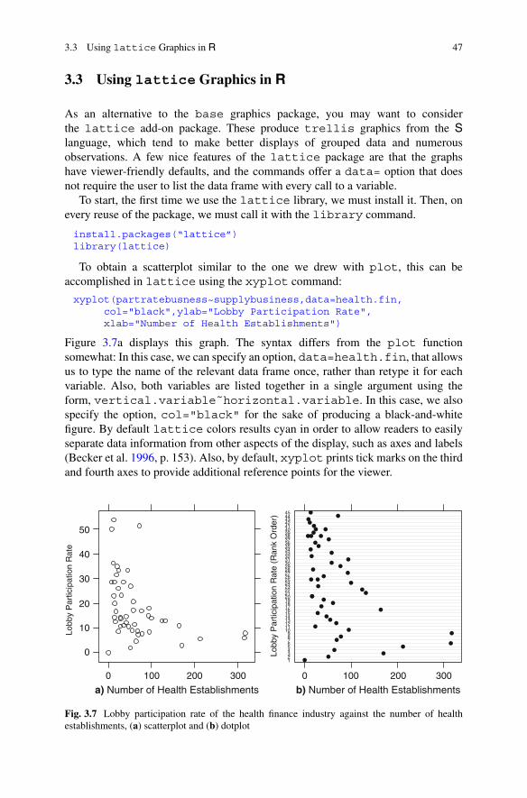
3.3 Using lattice Graphics in R 47
3.3 Using lattice Graphics in R
As an alternative to the base graphics package, you may want to considerthe lattice add-on package. These produce trellis graphics from the Slanguage, which tend to make better displays of grouped data and numerousobservations. A few nice features of the lattice package are that the graphshave viewer-friendly defaults, and the commands offer a data= option that doesnot require the user to list the data frame with every call to a variable.
To start, the first time we use the lattice library, we must install it. Then, onevery reuse of the package, we must call it with the library command.
install.packages(“lattice”)library(lattice)
To obtain a scatterplot similar to the one we drew with plot, this can beaccomplished in lattice using the xyplot command:
xyplot(partratebusness~supplybusiness,data=health.fin,col="black",ylab="Lobby Participation Rate",xlab="Number of Health Establishments")
Figure 3.7a displays this graph. The syntax differs from the plot functionsomewhat: In this case, we can specify an option, data=health.fin, that allowsus to type the name of the relevant data frame once, rather than retype it for eachvariable. Also, both variables are listed together in a single argument using theform, vertical.variable˜horizontal.variable. In this case, we alsospecify the option, col="black" for the sake of producing a black-and-whitefigure. By default lattice colors results cyan in order to allow readers to easilyseparate data information from other aspects of the display, such as axes and labels(Becker et al. 1996, p. 153). Also, by default, xyplot prints tick marks on the thirdand fourth axes to provide additional reference points for the viewer.
a) Number of Health Establishments
Lobb
y P
artic
ipat
ion
Rat
e
0
10
20
30
40
50
0
b) Number of Health Establishments
Lobb
y P
artic
ipat
ion
Rat
e (R
ank
Ord
er)
123456789
101112131415161718192021222324252627282930313233343536373839404142434445
300100 200 0 300100 200
Fig. 3.7 Lobby participation rate of the health finance industry against the number of healthestablishments, (a) scatterplot and (b) dotplot

48 3 Visualizing Data
Television Stories
Den
sity
0.000
0.005
0.010
0.015
0
a) Density plotP
erce
nt o
f Tot
al
0
10
20
30
40
b) Histogram
50 100 150 200 250Television Stories
0 50 100 150 200 250
Fig. 3.8 (a) Density plot and (b) histogram showing the univariate distribution of the monthlycount of television news stories related to energy
The lattice package also contains functions that draw graphs that are similarto a scatterplot, but instead use a rank-ordering of the vertical axis variable. This ishow the stripplot and dotplot commands work, and they offer another viewof a relationship and its robustness. The dotplot command may be somewhatmore desirable as it also displays a line for each rank-ordered value, offering a sensethat the scale is different. The dotplot syntax looks like this:
dotplot(partratebusness~supplybusiness,data=health.fin,col="black",ylab="Lobby Participation Rate (Rank Order)",xlab="Number of Health Establishments")
Figure 3.7b displays this result. The stripplot function uses similar syntax.Lastly, the lattice library again gives us an option to look at the distribution
of a single variable by plotting either a histogram or a density plot. Returning to thepresidential time series data we first loaded in Sect. 3.1, we can now draw a densityplot using the following line of code:
densityplot(~Energy,data=pres.energy,xlab="Television Stories",col="black")
This is presented in Fig. 3.8a. This output shows points scattered along the base,each representing the value of an observation. The smoothed line across the graphrepresents the estimated relative density of the variable’s values.
Alternatively, a histogram in lattice can be drawn with the histogramfunction:
histogram(~Energy, data=pres.energy,xlab="Television Stories", col="gray60")
This is printed in Fig. 3.8b. In this case, color is set to col="gray60".The default again is for cyan-colored bars. For a good grayscale option in

3.4 Graphic Output 49
this case, a medium gray still allows each bar to be clearly distinguished.A final interesting feature of histogram is left to the reader: The func-tion will draw conditional histogram distributions. If you still have thepost.nixon variable available that we created earlier, you might try typinghistogram(˜Energy|post.nixon,data=pres.energy), where thevertical pipe (|) is followed by the conditioning variable.
3.4 Graphic Output
A final essential point is a word on how users can export their R graphs into adesired word processor or desktop publisher. The first option is to save the screenoutput of a figure. On Mac machines, user may select the figure output windowand then use the dropdown menu File!Save As. . . to save the figure as a PDF file.On Windows machines, a user can simply right-click on the figure output windowitself and then choose to save the figure as either a metafile (which can be used inprograms such as Word) or as a postscript file (for use in LATEX). Also by right-clicking in Windows, users may copy the image and paste it into Word, PowerPoint,or a graphics program.
A second option allows users more precision over the final product. Specifically,the user can write the graph to a graphics device, of which there are several options.For example, in writing this book, I exported Fig. 3.5a by typing:
postscript("lin.partrate.eps",horizontal=FALSE,width=3,height=3,onefile=FALSE,paper="special",pointsize=7)
plot(y=health.fin$partratebusness,x=health.fin$supplybusiness,ylab="Lobby Participation Rate",xlab="Number of Health Establishments")
abline(finance.linear)dev.off()
The first line calls the postscript command, which created a file calledlin.partrate.eps that I saved the graph as. Among the key options in thiscommand are width and height, each of which I set to three inches. Thepointsize command shrank the text and symbols to neatly fit into the spaceI allocated. The horizontal command changes the orientation of the graphicfrom landscape to portrait orientation on the page. Change it to TRUE to have thegraphic adopt a landscape orientation. Once postscript was called, all graphingcommands wrote to the file and not to the graphing window. Hence, it is typically agood idea to perfect a graph before writing it to a graphics device. Thus, the plotand abline commands served to write all of the output to the file. Once I wasfinished writing to the file, the dev.off() command closed the file so that noother graphing commands would write to it.
Of course postscript graphics are most frequently used by writers who use thedesktop publishing language of LATEX. Writers who use more traditional wordprocessors such as Word or Pages will want to use other graphics devices. The
50 3 Visualizing Data
available options include: jpeg, pdf, png, and tiff.5 To use any of these fourgraphics devices, substitute a call for the relevant function where postscriptis in the previous code. Be sure to type ?png to get a feel for the syntax of thesealternative devices, though, as each of the five has a slightly different syntax.
As a special circumstance, graphs drawn from the lattice package use adifferent graphics device, called trellis.device. It is technically possible touse the other graphics devices to write to a file, but unadvisable because the deviceoptions (e.g., size of graph or font size) will not be passed to the graph. In the caseof Fig. 3.7b, I generated the output using the following code:
trellis.device("postscript",file="dotplot.partrate.eps",theme=list(fontsize=list(text=7,points=7)),horizontal=FALSE,width=3,height=3,onefile=FALSE,paper="special")
dotplot(partratebusness~supplybusiness,data=health.fin,col=’black’,ylab="Lobby Participation Rate (Rank Order)",xlab="Number of Health Establishments")
dev.off()
The first argument of the trellis.device command declares which driver theauthor wishes to use. Besides postscript, the author can use jpeg, pdf, orpng. The second argument lists the file to write to. Font and character size mustbe set through the theme option, and the remaining arguments declare the otherpreferences about the output.
This chapter has covered univariate and bivariate graphing functions in R.Several commands from both the base and lattice packages have beenaddressed. This is far from an exhaustive list of R’s graphing capabilities, andusers are encouraged to learn more about the available options. This primer should,however, serve to introduce users to various means by which data can be visualizedin R. With a good sense of how to get a feel for our data’s attributes visually, thenext chapter turns to numerical summaries of our data gathered through descriptivestatistics.
3.5 Practice Problems
In addition to their analysis of energy policy coverage introduced in this chapter,Peake and Eshbaugh-Soha (2008) also study drug policy coverage. These datasimilarly count the number of nightly television news stories in a month focusingon drugs, from January 1977 to December 1992. Their data is saved in comma-separated format in the file named drugCoverage.csv. Download their datafrom the Dataverse named on page vii or the chapter content link on page 33. Thevariables in this data set are: a character-based time index showing month and year
5My personal experience indicates that png often looks pretty clear and is versatile.

3.5 Practice Problems 51
(Year), news coverage of drugs (drugsmedia), an indicator for a speech on drugsthat Ronald Reagan gave in September 1986 (rwr86), an indicator for a speechGeorge H.W. Bush gave in September 1989 (ghwb89), the president’s approvalrating (approval), and the unemployment rate (unemploy).
1. Draw a histogram of the monthly count of drug-related stories. You may useeither of the histogram commands described in the chapter.
2. Draw two boxplots: One of drug-related stories and another of presidentialapproval. How do these figures differ and what does that tell you about thecontrast between the variables?
3. Draw two scatterplots:
(a) In the first, represent the number of drug-related stories on the vertical axis,and place the unemployment rate on the horizontal axis.
(b) In the second, represent the number of drug-related stories on the verticalaxis, and place presidential approval on the horizontal axis.
(c) How do the graphs differ? What do they tell you about the data?(d) Bonus: Add a linear regression line to each of the scatterplots.
4. Draw two line graphs:
(a) In the first, draw the number of drug-related stories by month over time.(b) In the second, draw presidential approval by month over time.(c) What can you learn from these graphs?
5. Load the lattice library and draw a density plot of the number of drug-relatedstories by month.
6. Bonus: Draw a bar graph of the frequency of observed unemployment rates.(Hint: Try using the table command to create the object you will graph.) Canyou go one step further and draw a bar graph of the percentage of time each valueis observed?

Chapter 4Descriptive Statistics
Before developing any models with or attempting to draw any inferences from adata set, the user should first get a sense of the features of the data. This can beaccomplished through the data visualization methods described in Chap. 3, as wellas through descriptive statistics of a variable’s central tendency and dispersion,described in this chapter. Ideally, the user will perform both tasks, regardlessof whether the results become part of the final published product. A traditionalrecommendation to analysts who estimate functions such as regression models isthat the first table of the article ought to describe the descriptive statistics of allinput variables and the outcome variable. While some journals have now turnedaway from using scarce print space on tables of descriptive statistics, a good dataanalyst will always create this table for him or herself. Frequently this informationcan at least be reported in online appendices, if not in the printed version of thearticle.
As we work through descriptive statistics, the working example in this chapterwill be policy-focused data from LaLonde’s (1986) analysis of the National Sup-ported Work Demonstration, a 1970s program that helped long-term unemployedindividuals find private sector jobs and covered the labor costs of their employmentfor a year. The variables in this data frame are:
treated: Indicator variable for whether the participant received the treatment.age: Measured in years.education: Years of education.black: Indicator variable for whether the participant is African-American.married: Indicator variable for whether the participant is married.nodegree: Indicator variable for not possessing a high school diploma.
Electronic supplementary material: The online version of this chapter(doi: 10.1007/978-3-319-23446-5_4) contains supplementary material, which is available toauthorized users.
© Springer International Publishing Switzerland 2015J.E. Monogan III, Political Analysis Using R, Use R!,DOI 10.1007/978-3-319-23446-5_4
53

54 4 Descriptive Statistics
re74: Real earnings in 1974.re75: Real earnings in 1975.re78: Real earnings in 1978.hispanic: Indicator variable for whether the participant is Hispanic.u74: Indicator variable for unemployed in 1974.u75: Indicator variable for unemployed in 1975.
4.1 Measures of Central Tendency
Our first task will be to calculate centrality measures, which give us a sense of atypical value of a distribution. The most common measures of central tendency arethe mean, median, and mode. The inter-quartile range, offering the middle 50 %of the data, is also informative. To begin with some example calculations, we firstmust load LaLonde’s data (named LL). These are available as part of the CoarsenedExact Matching package (cem), which we will discuss at greater length in Chap. 8.As with any other user-defined package, our first task is to install the package:
install.packages("cem")library(cem)data(LL)
After installing the package, we load the library, as we will have to do in everysession in which we use the package. Once the library is loaded, we can load thedata simply by calling the data command, which loads this saved data frame fromthe cem package into working memory. We conveniently can refer to the data frameby the name LL1.
For all of the measures of central tendency that we compute, suppose we havea single variable x, with n different values: x1; x2; x3; : : : ; xn. We also could sort thevalues from smallest to largest, which is designated differently with order statisticsas: x.1/; x.2/; x.3/; : : : x.n/. In other words, if someone asked you for the second orderstatistic, you would tell them the value of x.2/, the second smallest value of thevariable.
With a variable like this, the most commonly used measure of centrality is thesample mean. Mathematically, we compute this as the average of the observedvalues:
Nx D x1 C x2 C � � � C xn
nD 1
n
nX
iD1
xi (4.1)
Within R, we can apply Eq. (4.1)’s formula using the mean function. So if x in thiscase was the income participants in the National Supported Work Demonstrationearned in 1974, we would apply the function to the variable re74:
1These data also are available in comma-separated format in the file named LL.csv. This data filecan be downloaded from the Dataverse on page vii or the chapter content link on page 53.

4.1 Measures of Central Tendency 55
0 10000 20000
Income in 1974
N = 722 Bandwidth = 938.5
Den
sity
0.00
000
0.00
005
0.00
010
0.00
015
0.00
020
30000 40000
Fig. 4.1 Density plot of real earnings in 1974 from the National Supported Work Demonstrationdata
mean(LL$re74)
R responds by printing [1] 3630.738, so we can report the sample mean asNx D 3630:738.
Of course, it is advisable to continue to visualize the data using the tools fromChap. 3. Besides computing the mean of real earnings in 1974, we also can learna lot just from drawing a density plot. We could do this using the lattice codedescribed in the last chapter or with a little more user control as follows:
dens.74<-density(LL$re74,from=0)plot(dens.74,main="Income in 1974")abline(v=mean(LL$re74),col="red")
On the first line, the density command allows us to compute the density ofobservations at each value of income. With the from option, we can specify thatthe minimum possible value of income is 0 (and the to option would have let us seta maximum). On the second line, we simply plot this density object. Lastly, we useabline to add a vertical line where our computed mean of $3,630.74 is located.
The resulting graph is shown in Fig. 4.1. This figure is revealing: The bulk ofthe data fall below the mean. The mean is as high as it is because a handful of verylarge incomes (shown in the long right tail of the graph) are drawing it upward. Withthe picture, we quickly get a sense of the overall distribution of the data.
Turning back to statistical representations, another common measure of centraltendency is the sample median. One advantage of computing a median is that it ismore robust to extreme values than the mean. Imagine if our sample had somehowincluded Warren Buffett—our estimate of mean income would have increased

56 4 Descriptive Statistics
substantially just with one observation. The median, by contrast, would move verylittle in response to such an extreme observation. Our formula for computing amedian with observed data turns to the order statistics we defined above:
Qx D8<
:x�
nC12
� where n is odd
12
�x. n
2 / C x.1C n2 /
�where n is even
(4.2)
Note that notation for the median is somewhat scattered, and Qx is one of the severalcommonly used symbols. Formally, whenever we have an odd number of values, wesimply take the middle order statistic (or middle value when the data are sorted fromsmallest to largest). Whenever we have an even number of values, we take the twomiddle order statistics and average between them. (E.g., for ten observations, splitthe difference between x.5/ and x.6/ to get the median.) R will order our data, findthe middle values, and take any averages to report the median if we simply type:
median(LL$re74)
In this case, R prints [1] 823.8215, so we can report Qx D 823:8215 as themedian income for program participants in 1974. Observe that the median value ismuch lower than the mean value, $2,806.92 lower, to be exact. This is consistentwith what we saw in Fig. 4.1: We have a positive skew to our data, with someextreme values pulling the mean up somewhat. Later, we will further verify thisby looking at quantiles of our distribution.
A third useful measure of central tendency reports a range of central values.The inter-quartile range is the middle 50 % of the data. Using order statistics, wecompute the lower and upper bounds of this quantity as:
IQRx Dhx. n
4 /; x. 3n4 /
i(4.3)
The two quantities reported are called the first and third quartiles. The first quartileis a value for which 25 % of the data are less than or equal to the value. Similarly,75 % of the data are less than or equal to the third quartile. In this way, the middle50 % of the data falls between these two values. In R, there are two commands wecan type to get information on the inter-quartile range:
summary(LL$re74)IQR(LL$re74)
The summary command is useful because it presents the median and mean of thevariable in one place, along with the minimum, maximum, first quartile, and thirdquartile. Our output from R looks like this:
Min. 1st Qu. Median Mean 3rd Qu. Max.0.0 0.0 823.8 3631.0 5212.0 39570.0
This is handy for getting three measures of central tendency at once, though notethat the values of the mean and median by default are rounded to fewer digits that theseparate commands reported. Meanwhile, the interquartile range can be read from

4.1 Measures of Central Tendency 57
the printed output as IQRx D Œ0; 5212�. Normally, we would say that at least 50 % ofparticipants had an income between $0 and $5212. In this case, though, we know noone earned a negative income, so 75 % of respondents fell into this range. Finally,the IQR command reports the difference between the third and first quartiles, in thiscase printing: [1] 5211.795. This command, then, simply reports the spreadbetween the bottom and top of the interquartile range, again with less rounding thatwe would have gotten by using the numbers reported by summary.
In most circumstances, rounding and the slight differences in outputs that thesecommands produce pose little issue. However, if more digits are desired, the usercan control a variety of global options that shape the way R presents results withthe options command that was mentioned in Chap. 1. The digits argumentspecifically shapes the number of digits presented. So, for example, we could type:
options(digits=9)summary(LL$re74)
Our output would then look like this:
Min. 1st Qu. Median Mean 3rd Qu. Max.0.000 0.000 823.822 3630.740 5211.790 39570.700
Hence, we can see that discrepancies are a function of rounding. Bear in mind,though, that changes with the options command apply to all outputs in thesession. For instance, it turns out that if we re-ran the mean command the outputwould now show even more digits than we had before.
We also could get a general summary of all variables in a data set at once just bytyping the name of the data frame alone into the summary command:
summary(LL)
This reports the same descriptive statistics as before, but for all variables at once. Ifany observations are missing a value for a variable, this command will print thenumber of NA values for the variable. Beware, though, not all of the quantitiesreported in this table are meaningful. For indicator variables such as treated, black,married, nodegree, hispanic, u74, and u75, remember that the variables are notcontinuous. The mean essentially reports the proportion of respondents receiving a1 rather than a 0, and the count of any missing values is useful. However, the otherinformation is not particularly informative.
4.1.1 Frequency Tables
For variables that are measured nominally or ordinally, the best summary ofinformation is often a simple table showing the frequency of each value. In R,the table command reports this for us. For instance, our data include a simpleindicator coded 1 if the respondent is African-American and 0 otherwise. To get therelative frequencies of this variable, we type:

58 4 Descriptive Statistics
table(LL$black)
This prints the output:
0 1144 578
Hence, 144 respondents are not African-American, and 578 respondents areAfrican-American. With a nominal indicator such as this, the only valid measureof central tendency is the mode, which is the most common value a variable takeson. In this case, the most frequent value is a 1, so we could say that the mode isAfrican-American.
As another example, these data measure education in years. Measured in thisway, we could think of this as a continuous variable. Yet, the number of values thisvariable takes on is somewhat limited, as no one in the sample has fewer than threeor more than 16 years of education. We therefore may wish to look at a frequencytable for this variable as well. Also, even if the mean and the median are informativevalues, we may wish to compute the mode to know what the most common numberof years of education is in these data. To compute the frequency table and to have Rautomatically return the mode, we type:
table(LL$education)which.max(table(LL$education))
The table we see is:
3 4 5 6 7 8 9 10 11 12 13 14 15 161 6 5 7 15 62 110 162 195 122 23 11 2 1
At a glance, few respondents never went to high school at all, and only a handfulhave more than a high school education. We also could scan the table to observethat the mode is 11 years of education, which describes 195 respondents. However,if we have many more categories than we do for education, doing this will becomedifficult. Hence, feeding our table into the which.max command returns whichlabel in the table that has the maximum frequency. Our resulting printout is:
119
The first line, 11, prints the value label of the cell with the highest frequency—thisis our mode. The second line adds the additional detail that the value of 11 is theninth cell of the table (a detail we usually can ignore).
Another way we could present our frequencies is in a bar plot based on the abovetable. We could do this with the following code:
barplot(table(LL$education),xlab="Years of Education",ylab="Frequency",cex.axis=.9,cex.names=.9,ylim=c(0,200))
abline(h=0,col=’gray60’)box()
On the first line, we specify that we are drawing a bar plot of table(LL$education). Notice that we use cex.axis and cex.names to reduce the size
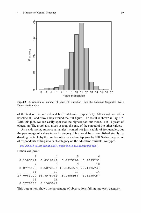
4.1 Measures of Central Tendency 59
Years of Education3 4 5 7 8 9 10 11 12 13 14 15 16 176
Fre
quen
cy
150
100
200
500
Fig. 4.2 Distribution of number of years of education from the National Supported WorkDemonstration data
of the text on the vertical and horizontal axis, respectively. Afterward, we add abaseline at 0 and draw a box around the full figure. The result is shown in Fig. 4.2.With this plot, we can easily spot that the highest bar, our mode, is at 11 years ofeducation. The graph also gives us a quick sense of the spread of the other values.
As a side point, suppose an analyst wanted not just a table of frequencies, butthe percentage of values in each category. This could be accomplished simply bydividing the table by the number of cases and multiplying by 100. So for the percentof respondents falling into each category on the education variable, we type:
100*table(LL$education)/sum(table(LL$education))
R then will print:
3 4 5 60.1385042 0.8310249 0.6925208 0.9695291
7 8 9 102.0775623 8.5872576 15.2354571 22.4376731
11 12 13 1427.0083102 16.8975069 3.1855956 1.5235457
15 160.2770083 0.1385042
This output now shows the percentage of observations falling into each category.

60 4 Descriptive Statistics
4.2 Measures of Dispersion
Besides getting a sense of the center of our variable, we also would like to knowhow spread out our observations are. The most common measures of this are thevariance and standard deviation, though we also will discuss the median averagedeviation as an alternative measure. Starting with the sample variance, our formulafor this quantity is:
Var.x/ D s2x D .x1 � Nx/2 C .x2 � Nx/2 C � � � C .xn � Nx/2
n � 1D 1
n � 1
nX
iD1
.xi � Nx/2
(4.4)
In R, we obtain this quantity with the function var. For income in 1974, we type:
var(LL$re74)
This prints the value: [1] 38696328. Hence, we can write Var.x/ D 38696328.Of course, the variance is in a squared metric. Since we may not want to think ofthe spread in terms of “38.7 million squared dollars,” we will turn to alternativemeasures of dispersion as well. That said, the variance is an essential quantity thatfeeds into a variety of other calculations of interest.
The standard deviation is simply the square root of the variance:
SD.x/ D sx Dp
Var.x/ Dvuut 1
n � 1
nX
iD1
.xi � Nx/2 (4.5)
This simple transformation of the variance has the nice property of putting ourmeasure of dispersion back onto the original scale. We could either take the squareroot of a computed variance, or allow R to do all steps of the calculation for us:
sd(LL$re74)
In this case, R prints: [1] 6220.637. Hence, sx D 6220:637. When a variableis shaped like a normal distribution (which our income variable is not), a usefulapproximation is the 68-95-99.7 rule. This means that approximately 68 % of ourdata fall within one standard deviation of the mean, 95 % within two standarddeviations, and 99.7 % within three standard deviations. For income in 1974, a heavyconcentration of incomes at $0 throws this rule off, but with many other variables itwill observationally hold.
A very different measure of dispersion is the median absolute deviation. Wedefine this as:
MAD.x/ D median.jxi � median.x/j/ (4.6)
In this case, we use the median as our measure of centrality, rather than the mean.Then we compute the absolute difference between each observation and the median.Lastly, we compute the median of the deviations. This offers us a sense of a typicaldeviation from the median. In R the command is typed:
mad(LL$re74)

4.2 Measures of Dispersion 61
Here, R returns a value of 1221.398. Like the standard deviation, this is on thescale of the original variable, in dollars. Unlike the standard deviation, this statisticturns out to be much smaller in this case. Again, extreme values can really run-up variances and standard deviations, just as they can distort a mean. The medianabsolute deviation, by contrast, is less sensitive to extreme values.
4.2.1 Quantiles and Percentiles
As a final topic, quantiles and percentiles allow us to gain a sense of a variable’soverall distribution. Quantiles are the relative placement of data values in a sortedlist, scaled Œ0; 1�. For a value q the quantile for that value would be the orderstatistic x.q�n/. Percentiles are the same thing, scaled Œ0; 100�, so for a value p thepth percentile would be x. p�n
100 /. Hence, the median is the 0.5 quantile and the 50thpercentile. Special cases of quantiles include the previously introduced quartiles(dividing the data into four groups), quintiles (dividing into five groups), and deciles(dividing into ten groups).
In R, the command quantile can give us any quantile we wish. By default,R prints the quantiles for q 2 f0:00; 0:25; 0:50; 0:75; 1:00g. We have the option ofspecifying whichever quantiles we want, though. The syntax is:
quantile(LL$re74)quantile(LL$re74, c(0,.1,.2,.3,.4,.5,.6,.7,.8,.9,1))
The first command prints our default quantiles, though it reports them with therescaled percentile labels:
0% 25% 50% 75% 100%0.0000 0.0000 823.8215 5211.7946 39570.6797
Essentially, this information repeats the quartile information that summary pro-vided us earlier. On our second line of code, we add a vector of 11 quantiles ofinterest to request deciles, which give us the cut points for each additional 10 % ofthe data. This result is:
0% 10% 20% 30%0.0000 0.0000 0.0000 0.0000
40% 50% 60% 70%0.0000 823.8215 1837.2208 3343.5705
80% 90% 100%6651.6747 10393.2177 39570.6797
This is revealing as it shows that at least 40 % of our respondents had an incomeof $0 in 1974. Further, going from the 90th percentile to the 100th percentile(or maximum), we see a jump from $10,393 to $39,570, suggesting that someparticularly extreme values are in the top 10 % of our data. Hence, these data do
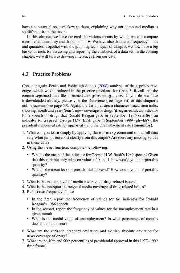
62 4 Descriptive Statistics
have a substantial positive skew to them, explaining why our computed median isso different from the mean.
In this chapter, we have covered the various means by which we can computemeasures of centrality and dispersion in R. We have also discussed frequency tablesand quantiles. Together with the graphing techniques of Chap. 3, we now have a bigbasket of tools for assessing and reporting the attributes of a data set. In the comingchapter, we will turn to drawing inferences from our data.
4.3 Practice Problems
Consider again Peake and Eshbaugh-Soha’s (2008) analysis of drug policy cov-erage, which was introduced in the practice problems for Chap. 3. Recall that thecomma-separated data file is named drugCoverage.csv. If you do not haveit downloaded already, please visit the Dataverse (see page vii) or this chapter’sonline content (see page 53). Again, the variables are: a character-based time indexshowing month and year (Year), news coverage of drugs (drugsmedia), an indicatorfor a speech on drugs that Ronald Reagan gave in September 1986 (rwr86), anindicator for a speech George H.W. Bush gave in September 1989 (ghwb89), thepresident’s approval rating (approval), and the unemployment rate (unemploy).
1. What can you learn simply by applying the summary command to the full dataset? What jumps out most clearly from this output? Are there any missing valuesin these data?
2. Using the mean function, compute the following:
• What is the mean of the indicator for George H.W. Bush’s 1989 speech? Giventhat this variable only takes on values of 0 and 1, how would you interpret thisquantity?
• What is the mean level of presidential approval? How would you interpret thisquantity?
3. What is the median level of media coverage of drug-related issues?4. What is the interquartile range of media coverage of drug-related issues?5. Report two frequency tables:
• In the first, report the frequency of values for the indicator for RonaldReagan’s 1986 speech.
• In the second, report the frequency of values for the unemployment rate in agiven month.
• What is the modal value of unemployment? In what percentage of monthsdoes the mode occur?
6. What are the variance, standard deviation, and median absolute deviation fornews coverage of drugs?
7. What are the 10th and 90th percentiles of presidential approval in this 1977–1992time frame?

Chapter 5Basic Inferences and Bivariate Association
In this chapter, we begin to use inferential statistics and bivariate statistics.In Chap. 4, we were content simply to characterize the properties of a single variablein the sample at hand. Usually in Political Science, though, our motivation asresearchers will be to argue whether a claim can be generalized. Hence, inferentialstatistics are designed to draw inferences about a broader population. Further, wefrequently want to measure the level of association between variables, and bivariatestatistics serve as measures of the degree to which two variables are associated witheach other.
In later chapters, linear regression models, generalized linear models, timeseries models, and other models that we estimate offer the opportunity to drawan inference about a broader population. They also allow us to evaluate bivariateor multivariate relationships among variables. For now, we focus on a handful ofstepping stone inferential and bivariate statistics: Tests about means, associationsbetween two categorical variables (via cross-tabulations), and correlations betweentwo continuous variables.
In this chapter, our working example data will be the same data from LaLonde’s(1986) analysis of the National Supported Work Demonstration. Information aboutthe features of these data can be reviewed at the start of Chap. 4. In this case,every member of our sample is someone who was long-term unemployed. Hence, aswe draw inferences, it would not be fair to try to conclude something about the entirepopulation of the USA in the mid-1970s because these data do not compose a sampleof that population. For the purposes of our working example, we will attempt to drawconclusions about the population of long-term unemployed persons in the USA.More information on how this sample was drawn is available in LaLonde (1986),
Electronic supplementary material: The online version of this chapter(doi: 10.1007/978-3-319-23446-5_5) contains supplementary material, which is available toauthorized users.
© Springer International Publishing Switzerland 2015J.E. Monogan III, Political Analysis Using R, Use R!,DOI 10.1007/978-3-319-23446-5_5
63

64 5 Basic Inferences and Bivariate Association
and the reader is urged to read about random sampling if more information is desiredabout the theory of statistical inference.
5.1 Significance Tests for Means
Before computing any inferential statistics, we must load LaLonde’s data onceagain. Users who have already installed the cem library can simply type:
library(cem)data(LL)
Users who did not install cem in Chap. 4 will need to type install.packages("cem") before the two preceding lines of code will work properly. Once thesedata are loaded in memory, again by the name LL, we can turn to applied analysis1.
We begin by testing hypotheses about the mean of a population (or multiplepopulations). We first consider the case where we want to test whether the meanof some population of interest differs from some value of interest. To conduct thissignificance test, we need: (1) our estimate of the sample mean, (2) the standarderror of our mean estimate, and (3) a null and alternative hypothesis. The samplemean is defined earlier in Eq. (4.1), and the standard error of our estimate is simplythe standard deviation of the variable [defined in Eq. (4.5)] divided by the squareroot of our sample size, sx=
pn.
When defining our null and alternative hypotheses, we define the null hypothesisbased on some value of interest that we would like to rule out as a possible value ofthe population parameter. Hence, if we say:
H0 W � D �0
This means that our null hypothesis (H0) is that the population mean (�) is equalto some numeric value we set (�0). Our research hypothesis is the alternativehypothesis we would like to reject this null in favor of. We have three choices forpotential research hypotheses:
HA W � > �0
HA W � < �0
HA W � ¤ �0
The first two are called one-tailed tests and indicate that we believe the populationmean should be, respectively, greater than or less than the proposed value �0. Mostresearch hypotheses should be considered as one of the one-tailed tests, thoughoccasionally the analyst does not have a strong expectation on whether the mean
1As before, these data also are available in comma-separated format in the file named LL.csv.This data file can be downloaded from the Dataverse on page vii or the chapter content link onpage 63.

5.1 Significance Tests for Means 65
should be bigger or smaller. The third alternative listed defines the two-tailed test,which asks whether the mean is simply different from (or not equal to) the value �0.
Once we have formulated our hypothesis, we compute a t-ratio as our test statisticfor the hypothesis. Our test statistic includes the sample mean, standard error, andthe population mean defined by the null hypothesis (�0). This formula is:
t D Nx � �0
SE.NxjH0/D Nx � �0
sx=p
n(5.1)
This is distributed Student’s-t with n � 1 degrees of freedom under the null(and asymptotically normal).2 Once we have this test statistic, we compute ourp-value as follows:
p � value D
8ˆ<
ˆ:
P.t� � tjH0/ HA W � < �0
P.t� � tjH0/ HA W � > �0
P.jt� � �0j � jt � �0jjH0/ HA W � ¤ �0
In this case, assume t� is the actual value of our statistic that we compute. Thetypical action in this case is to have a pre-defined confidence level and decidewhether to reject the null hypothesis or not based on whether the p-value indicatesthat rejection can be done with that level of confidence. For instance, if an analystwas willing to reject a null hypothesis if he or she could do so with 90 % confidence,then if p < 0:10, he or she would reject the null and conclude that the researchhypothesis is correct. Many users also proceed to report the p-value so that readerscan draw conclusions about significance themselves.
R makes all of these calculations very straightforward, doing all of this in a singleline of user code. Suppose that we had a hypothesis that, in 1974, the population oflong-term unemployed Americans had a lower income than $6,059, a governmentestimate of the mean income for the overall population of Americans. In this case,our hypothesis is:
H0 W � D 6059
HA W � < 6059
This is a one-tailed test because we do not even entertain the idea that the long-termunemployed could have an on-average higher income than the general population.Rather, we simply ask whether the mean of our population of interest is discerniblylower than $6,059 or not. To test this hypothesis in R, we type:
t.test(LL$re74, mu=6059, alternative="less")
2This statistic has a t distribution because the sample mean has a normally distributed samplingdistribution and the sample standard error has a �2 sampling distribution with n � 1 degrees offreedom. The ratio of these two distributions yields a t distribution.
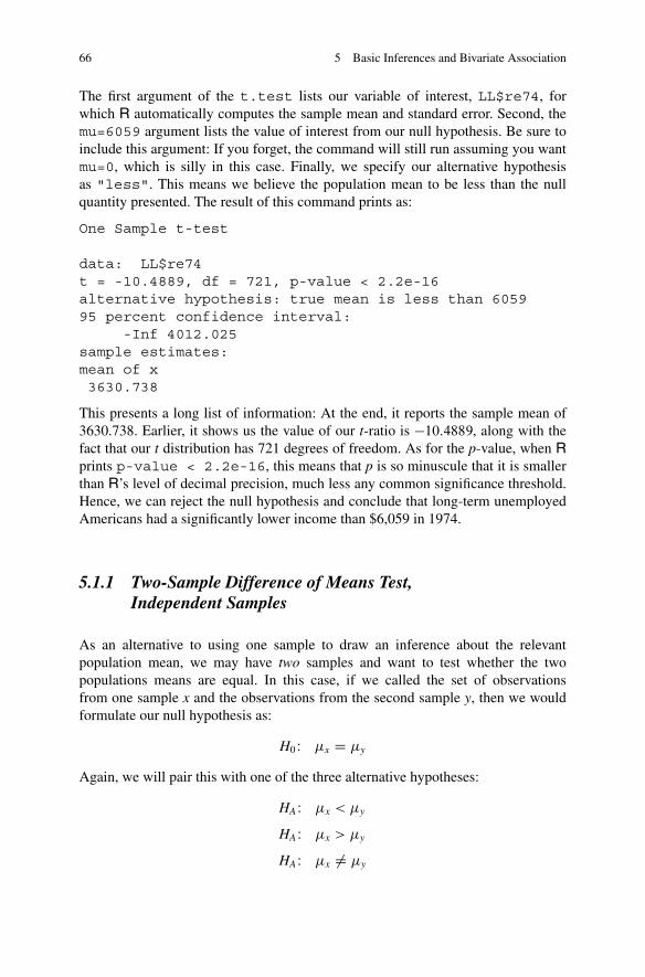
66 5 Basic Inferences and Bivariate Association
The first argument of the t.test lists our variable of interest, LL$re74, forwhich R automatically computes the sample mean and standard error. Second, themu=6059 argument lists the value of interest from our null hypothesis. Be sure toinclude this argument: If you forget, the command will still run assuming you wantmu=0, which is silly in this case. Finally, we specify our alternative hypothesisas "less". This means we believe the population mean to be less than the nullquantity presented. The result of this command prints as:
One Sample t-test
data: LL$re74t = -10.4889, df = 721, p-value < 2.2e-16alternative hypothesis: true mean is less than 605995 percent confidence interval:
-Inf 4012.025sample estimates:mean of x3630.738
This presents a long list of information: At the end, it reports the sample mean of3630.738. Earlier, it shows us the value of our t-ratio is �10:4889, along with thefact that our t distribution has 721 degrees of freedom. As for the p-value, when Rprints p-value < 2.2e-16, this means that p is so minuscule that it is smallerthan R’s level of decimal precision, much less any common significance threshold.Hence, we can reject the null hypothesis and conclude that long-term unemployedAmericans had a significantly lower income than $6,059 in 1974.
5.1.1 Two-Sample Difference of Means Test,Independent Samples
As an alternative to using one sample to draw an inference about the relevantpopulation mean, we may have two samples and want to test whether the twopopulations means are equal. In this case, if we called the set of observationsfrom one sample x and the observations from the second sample y, then we wouldformulate our null hypothesis as:
H0 W �x D �y
Again, we will pair this with one of the three alternative hypotheses:
HA W �x < �y
HA W �x > �y
HA W �x ¤ �y

5.1 Significance Tests for Means 67
Again, the first two possible alternative hypotheses are one-tailed tests where wehave a clear expectation as to which population’s mean should be bigger. Thethird possible alternative simply evaluates whether the means are different. Whenbuilding our test statistic from this null hypothesis, we rely on the fact that H0 alsoimplies �x � �y D 0. Using this fact, we construct our t-ratio as:
t D .Nx � Ny/ � .�x � �y/
SE.Nx � NyjH0/(5.2)
The last question is how we calculate the standard error. Our calculation dependson whether we are willing to assume that the variance is the same in each population.Under the assumption of unequal variance, we compute the standard error as:
SE.Nx � NyjH0/ Ds
s2x
nxC s2
y
ny(5.3)
Under the assumption of equal variance, we have:
SE.Nx � NyjH0/ Ds
.nx � 1/s2x C .ny � 1/s2
y
nx C ny � 2
s1
nxC 1
ny(5.4)
As an example, we can conduct a test with the last observation of income in theNational Supported Work Demonstration, which was measured in 1978. Supposeour hypothesis is that income in 1978 was higher among individuals who receivedthe treatment of participating in the program (y) than it was among those who werecontrol observations and did not get to participate in the program (x). Our hypothesisin this case is:
H0 W �x D �y
HA W �x < �y
Again, this is a one-tailed test because we are not entertaining the idea thatthe treatment could have reduced long-term income. Rather, the treatment eitherincreased income relative to the control observations, or it had no discernibleeffect. R allows us to conduct this two-sample t-test using either assumption. Thecommands for unequal and equal variances, respectively, are:
t.test(re78~treated,data=LL,alternative="less",var.equal=F)t.test(re78~treated,data=LL,alternative="less",var.equal=T)
The first argument, re78˜treated, is in functional notation and indicates thatincome in 1978 is being separated based on values of the treatment indicator.The data option allows us to name the dataset so that we do not have to callit for each variable. When we state alternative="less", we are declaringour alternative hypothesis to mean that the average income for the lower value of

68 5 Basic Inferences and Bivariate Association
treated (group 0, the control) should be lower than the average for the higher valueof treated (group 1, the treated group). The only difference between the commandsis that the first sets var.equal=F so that variances are assumed unequal, and thesecond sets var.equal=T so that variances are assumed equal.
The results print as follows. For the assumption of unequal variances, we see:
Welch Two Sample t-test
data: re78 by treatedt = -1.8154, df = 557.062, p-value = 0.035alternative hypothesis: true difference in means is less
than 095 percent confidence interval:
-Inf -81.94117sample estimates:mean in group 0 mean in group 1
5090.048 5976.352
Meanwhile for the equal variance assumption, we see:
Two Sample t-test
data: re78 by treatedt = -1.8774, df = 720, p-value = 0.03043alternative hypothesis: true difference in means is less
than 095 percent confidence interval:
-Inf -108.7906sample estimates:mean in group 0 mean in group 1
5090.048 5976.352
The results are pretty similar, as would be expected. Both report the same estimatesof the means for the control group (5090.048) and treated group (5976.352).However, because the standard error is computed differently, we get slightlydifferent t values in each case (and a differently calculated degrees of freedomfor the unequal variances). The p-value is slightly larger when assuming unequalvariances, but in this case either option yields a similar conclusion. Hence, in eithercase, we reject the null hypothesis at the 95 % confidence level and conclude thatfor the treated group income was higher in 1978 than for the control group. It shouldbe noted that one limitation of a test like this is that we have not controlled for anyof the other variables known to influence income, and the treatment assignment wasnot random in this case. Chapters 6–8 offer several examples of methods designedto control statistically for other predictors. Specifically, in Sect. 8.3 we revisit thisexact example with a more advanced technique.

5.1 Significance Tests for Means 69
5.1.2 Comparing Means with Dependent Samples
A third mean-related test statistic we may want to compute is a difference ofmeans with a dependent sample (e.g., comparing matched samples). In other words,suppose we have a situation in which each observation in sample 1 matches with anobservation in sample 2. This could mean we are studying the same person beforeand after an event, a person doing the same task with different treatments, usinga twin study, or using matching methods to pair treated observations to controlobservations. In this case, we should no longer treat each sample as independent,but compute differences for each pairing and analyze the differences. An easy wayto think of this would be to create a new variable, wi D xi � yi where x and y arematched for each case i. In this case, our null hypothesis is H0 W �w D 0, and ouralternative hypothesis can be any of the three choices:
HA W �w < 0
HA W �w > 0
HA W �w ¤ 0
The test statistic in this case is given by Eq. (5.5), computed for the new variable w.
t D Nw � 0
SE. NwjH0/D Nw
sw=p
n(5.5)
As can be seen, this is effectively the same test statistic as in Eq. (5.1) with w asthe variable of interest and 0 as the null value. The user technically could createthe w variable him or herself and then simply apply the code for a single-samplesignificance test for a mean.
More quickly, though, this procedure could be automated by inserting twoseparate variables for the linked observations into the t-test command. Suppose,for instance, that we wanted to know if our control observations saw a rise intheir income from 1974 to 1978. It is possible that wages may not increase overthis time because these numbers are recorded in real terms. However, if wages didincrease, then observing how they changed for the control group can serve as a goodbaseline for comparing change in the treated group’s wages in the same time frame.To conduct this paired sample t-test for our control observations, we type:
LL.0<-subset(LL,treated==0)t.test(LL.0$re74,LL.0$re78,paired=T,alternative="less")
In the first line we create a subset only of our control observations. In the secondline, our first argument is the measure of income in 1974, and the second is incomein 1978. Third, we specify the option paired=T: This is critical, otherwise R willassume each variable forms an independent sample, but in our case this is a pairedsample where each individual has been observed twice. (To this end, by typingpaired=F instead, this gives us the syntax for a two-sample t-test if our separate

70 5 Basic Inferences and Bivariate Association
samples are in differing columns of data.) Finally, alternative="less"meansthat we expect the mean of the first observation, in 1974, to be lower than the meanof the second, in 1978. Our results are:
Paired t-test
data: LL.0$re74 and LL.0$re78t = -3.8458, df = 424, p-value = 6.93e-05alternative hypothesis: true difference in means isless than 095 percent confidence interval:
-Inf -809.946sample estimates:mean of the differences
-1417.563
This output tells us that earnings were on average $1,417.56 lower in 1974 than in1978. Our t-ratio is t D �3:8458, and the corresponding p-value is p D 0:00007.Hence at any common confidence threshold, we can reject the null hypothesisand conclude that incomes were higher in 1978 than in 1974 among long-termunemployed who did not receive the treatment.
Just as a final comparison, we could compute the same sort of test on the treatedgroup as follows:
LL.1<-subset(LL,treated==1)t.test(LL.1$re74,LL.1$re78,paired=T,alternative="less")
The results are somewhat similar:
Paired t-test
data: LL.1$re74 and LL.1$re78t = -4.7241, df = 296, p-value = 1.788e-06alternative hypothesis: true difference in means isless than 095 percent confidence interval:
-Inf -1565.224sample estimates:mean of the differences
-2405.353
We observe a bigger growth of $2,405.35 among the treated observations, and thisresult is also statistically discernible. This larger growth rate is encouraging forthe long-term earnings potential of the program. For bonus points, the reader isencouraged to look up difference-in-differences techniques and consider how theymight apply to studies with a design such as this.

5.2 Cross-Tabulations 71
5.2 Cross-Tabulations
In situations where we want to analyze the association between two nominal orordinal variables, a cross-tabulation is often a good tool for inference. A crosstabulation tests the hypothesis that an independent categorical variable affectsthe conditional distribution of a dependent categorical variable. The researcherasks: Will certain values of the dependent variable be noticeably more or lessfrequent when moving from one category of an independent variable to another? Inassessing this effect, the analyst should always break down relative percentages ofcategories of the dependent variable within categories of the independent variable.Many people make a mistake by breaking down percentages within categories ofthe dependent variable; such a mistake prevents a researcher from substantivelyevaluating the stated hypothesis that the independent variable causes the dependentvariable and not the reverse. The results of a cross-tabulation substantively comparethe percentages of the same value of the dependent variable across categories of theindependent variable.
Some common mistakes to avoid: First, once again, avoid breaking down per-centages by the dependent variable. Second, avoid comparing the largest percentagein each category of an independent variable. The hypothesis states that the frequencyof the dependent variable will vary by value of the independent variable; it does notargue what value of the dependent variable will be most frequent. Lastly, avoiddrawing inferences based on the pure magnitude of percentages; the researcher’stask is to look at differences in the distribution. For example, if vote choice is thedependent variable, and 66 % of Republicans support the Democratic candidate,while 94 % of Democrats support the Democratic candidate, the researcher shouldnot focus on majority support from both parties. Instead, the researcher shouldobserve that a 28 percentage point difference implies that partisanship has animportant effect on how individuals vote.
Consider two examples from the LaLonde dataset. First, we can simply askwhether being unemployed in 1974 (u74) served as a good predictor of beingunemployed in 1975 (u75). We would have to think that an individual’s prior workstatus shapes current work status. To build a cross-tabulation in R we need to installthe gmodels package and then load the library. Once we have done this, we canuse the CrossTable function:
install.packages(”gmodels”)library(gmodels)CrossTable(y=LL$u75,x=LL$u74,prop.c=F,prop.t=F,
prop.chisq=F,chisq=T,format="SPSS")
In this code, y specifies the column variable, and x specifies the row variable. Thismeans our dependent variable makes up the columns and the independent makes upthe rows. Because we want the conditional distribution of the dependent variablefor each given value of the independent variable, the options prop.c, prop.t,and prop.chisq are all set to FALSE (referring to proportion of the column,total sample, and contribution to the chisquare statistic). This means that each cell

72 5 Basic Inferences and Bivariate Association
only contains the raw frequency and the row-percentage, which corresponds to thedistribution conditional on the independent variable. The option chisq=T reportsPearson’s Chi-squared (�2) test. Under this test, the null hypothesis is that the twovariables are independent of each other. The alternative hypothesis is that knowingthe value of one variable changes the expected distribution of the other.3 By settingthe format option to SPSS, rather than SAS, we are presented with percentagesin our cells, rather than proportions.
The results of this command are printed below:
Cell Contents|-------------------------|| Count || Row Percent ||-------------------------|
Total Observations in Table: 722
| LL$u75LL$u74 | 0 | 1 | Row Total |
-------------|-----------|-----------|-----------|0 | 386 | 9 | 395 |
| 97.722% | 2.278% | 54.709% |-------------|-----------|-----------|-----------|
1 | 47 | 280 | 327 || 14.373% | 85.627% | 45.291% |
-------------|-----------|-----------|-----------|Column Total | 433 | 289 | 722 |-------------|-----------|-----------|-----------|
Statistics for All Table Factors
Pearson’s Chi-squared test-------------------------------------------------------Chi^2 = 517.7155 d.f. = 1 p = 1.329138e-114
Pearson’s Chi-squared test with Yates’ continuitycorrection-------------------------------------------------------Chi^2 = 514.2493 d.f. = 1 p = 7.545799e-114
Minimum expected frequency: 130.8906
3Note that this is a symmetric test of association. The test itself has no notion of which is thedependent or independent variable.

5.2 Cross-Tabulations 73
As we can see, among those who were employed in 1974 (u74=0), 97.7 % wereemployed in 1975. Among those who were unemployed in 1974 (u75=1), 14.4 %were employed in 1975.4 This corresponds to an 83.3 percentage point differencebetween the categories. This vast effect indicates that employment status in 1year does, in fact, beget employment status in the following year. Further, ourtest statistic is �2
1df D 517:7155 with a minuscule corresponding p-value. Hence,we reject the null hypothesis that employment status in 1974 is independent fromemployment status in 1975 and conclude that employment status in 1974 conditionsthe distribution of employment status in 1975.
As a more interesting question, we might ask whether receiving the treatmentfrom the National Supported Work Demonstration shapes employment status in1975. We would test this hypothesis with the code:
CrossTable(y=LL$u75,x=LL$treated,prop.c=F,prop.t=F,prop.chisq=F,chisq=T,format="SPSS")
The output from this command is:
Cell Contents|-------------------------|| Count || Row Percent ||-------------------------|
Total Observations in Table: 722
| LL$u75LL$treated | 0 | 1 | Row Total |
-------------|-----------|-----------|-----------|0 | 247 | 178 | 425 |
| 58.118% | 41.882% | 58.864% |-------------|-----------|-----------|-----------|
1 | 186 | 111 | 297 || 62.626% | 37.374% | 41.136% |
-------------|-----------|-----------|-----------|Column Total | 433 | 289 | 722 |-------------|-----------|-----------|-----------|
Statistics for All Table Factors
4To get more meaningful levels than 0 and 1 in this case, we would need to create copies of thevariables u74 and u75 that recorded each value as text (e.g., “Unemployed” and “Employed”). Therecode command from the car library offers a straightforward way of doing this, if desired.

74 5 Basic Inferences and Bivariate Association
Pearson’s Chi-squared test-------------------------------------------------------Chi^2 = 1.480414 d.f. = 1 p = 0.2237097
Pearson’s Chi-squared test with Yates’ continuitycorrection-------------------------------------------------------Chi^2 = 1.298555 d.f. = 1 p = 0.2544773
Minimum expected frequency: 118.8823
Substantively, the effects are in the expected direction. Among control observa-tions (treated=0), 58.1 % were employed in 1975. Among treated observations(treated=1), 62.6 % were employed in 1975. Hence we see a 4.5 percentagepoint bump in employment among treated observations over control observations.However, our test statistic is �2
1df D 1:4804. The corresponding p-value is p D0:2237. Hence, if we set our confidence threshold at 90 % or anything higher, wewould fail to reject the null hypothesis and conclude that there was no discerniblerelationship between the treatment and employment status.
5.3 Correlation Coefficients
As a preview to the next chapter, we conclude our look at bivariate statistics byshowing how to calculate a correlation coefficient in R. Correlation coefficients arecalculated as a measure of association between two continuous variables. We specif-ically focus on Pearson’s r, the correlation coefficient for a linear relationship.This value shows how well the independent variable linearly predicts the dependentvariable. This measure will range between �1 and 1. A correlation coefficient of 0suggests the absence of any linear relationship between the two variables. (Though,importantly, a nonlinear relationship also might yield r D 0 and some erroneousconclusions.) A value of 1 would imply a perfect positive relationship, and a valueof �1 would indicate a perfect negative relationship. The square of a Pearson’s r(r2) calculates the amount of variance explained by the predictor.
The formula for a Pearson correlation coefficient is essentially the covariance oftwo variables, x and y, divided by the standard deviation of each variable:
r DPn
iD1.xi � Nx/.yi � Ny/pPn
iD1.xi � Nx/pPn
iD1.yi � Ny/(5.6)

5.3 Correlation Coefficients 75
Within R, this quantity is computed with the cor command.5
Suppose we wanted to evaluate whether the number of years of education servedas a good predictor of our first measure of income, in 1974. We could type:
cor(LL$education,LL$re74)cor(LL$education,LL$re74)^2
The first line computes the actual correlation coefficient itself. R returns a printoutof: [1] 0.08916458. Hence, our correlation coefficient is r D 0:0892. Thesecond line recalculates the correlation and squares the result for us all at once.This tells us that r2 D 0:0080. The implication of this finding is that by knowing arespondent’s number of years of education, we could explain 0.8 % of the variancein 1974 income. On its face, this seems somewhat weak, but as a general word ofadvice always gauge r2 (or multiple R2, in the next chapter) values by comparingthem with other findings in the same area. Some sorts of models will routinelyexplain 90 % of the variance, while others do well to explain 5 % of the variance.
As a final example, we can consider the idea that income begets income. Considerhow well income in 1975 correlates with income in 1978. We compute this bytyping:
cor(LL$re75,LL$re78)cor(LL$re75,LL$re78)^2
The first line returns the correlation coefficient between these two variables,printing: [1] 0.1548982. Our estimate of r D 0:1549 indicates that high valuesof income in 1975 do generally correspond to high values of income in 1978. In thiscase, the second line returns r2 D 0:0240. This means we can explain 2.4 % of thevariance of income in 1978 by knowing what someone earned in 1975.
Remember that the graphing tools from Chap. 3 can help us understand our data,including any results that we quantify such as correlation coefficients. If we arewondering why earlier income does not do a better job of predicting later income,we could draw a scatterplot as follows:
plot(x=LL$re75,y=LL$re78,xlab="1975 Income",ylab="1978 Income",asp=1,xlim=c(0,60000),ylim=c(0,60000),pch=".")
Notice that we have used the asp=1 option to set the aspect ratio of the two axesat 1. This guarantees that the scale of the two axes is held to be the same—whichis appropriate since both variables in the figure are measured in inflation-adjusteddollars. The output is reported in Fig. 5.1. As can be seen, many of the observationscluster at zero in one or both of the years, so there is a limited degree to which alinear relationship characterizes these data.
We now have several basic inferences in hand: t-tests on means and �2 testsfor cross-tabulations. Difference in means tests, cross-tabulations, and correlation
5The cor command also provides a method option for which available arguments are pearson,kendall (which computes Kendall’s � , a rank correlation), and spearman (which computesSpearman’s �, another rank correlation). Users are encouraged to read about the alternate methodsbefore using them. Here, we focus on the default Pearson method.

76 5 Basic Inferences and Bivariate Association
0
0
1975 Income
1978
Inco
me
1000
020
000
3000
040
000
5000
060
000
10000 20000 30000 40000 50000 60000
Fig. 5.1 Scatterplot of income in 1975 and 1978 from National Supported Work Demonstrationdata
coefficients have also given us a good sense of evaluating bivariate relationships.In the next chapter, we turn to multivariate statistics, specifically using linearregression methods. This will build on the linear techniques that correlationcoefficients use and allow us to introduce the concept of statistical control.
5.4 Practice Problems
Please load the foreign library and download Alvarez et al.’s (2013) data, whichare saved in the Stata-formatted file alpl2013.dta. This file is available fromthe Dataverse named on page vii or the chapter content named on page 63. Thesedata are from a field experiment in Salta, Argentina in which some voters castballots through e-voting, and others voted in the traditional setting. The variablesare: an indictor for whether the voter used e-voting or traditional voting (EV), agegroup (age_group), education (educ), white collar worker (white_collar), not afull time worker (not_full_time), male (male), a count variable for number of sixpossible technological devices used (tech), an ordinal scale for political knowledge

5.4 Practice Problems 77
(pol_info), a character vector naming the polling place (polling_place), whether therespondent thinks poll workers are qualified (capable_auth), whether the voter eval-uated the voting experience positively (eval_voting), whether the voter evaluatedthe speed of voting as quick (speed), whether the voter is sure his or her vote is beingcounted (sure_counted), whether the voter thought voting was easy (easy_voting),whether the voter is confident in ballot secrecy (conf_secret), whether the voterthinks Salta’s elections are clean (how_clean), whether the voter thinks e-votingshould replace traditional voting (agree_evoting), and whether the voter prefersselecting candidates from different parties electronically (eselect_cand).
1. Consider the number of technological devices. Test the hypothesis that theaverage Salta voter has used more than three of these six devices. (Formally:H0 W � D 3I HA W � > 3.)
2. Conduct two independent sample difference of means tests:
a. Is there any difference between men and women in how many technologicaldevices they have used?
b. Is there any difference in how positively voters view the voting experience(eval_voting) based on whether they used e-voting or traditional voting (EV)?
3. Construct two cross-tabulations:
a. Construct a cross-tabulation where the dependent variable is how positivelyvoters view the voting experience (eval_voting) and the independent variableis whether they used e-voting or traditional voting (EV). Does the distributionof voting evaluation depend on whether the voter used e-voting? This cross-tabulation addressed the same question as is raised in #2.b. Which approachis more appropriate here?
b. Construct a cross-tabulation where the dependent variable is how positivelyvoters view the voting experience (eval_voting) and the independent variableis the ordinal scale of political knowledge (pol_info). Does the distribution ofvoting evaluation change with the voter’s level of political knowledge?
4. Consider the correlation between level of education (educ) and political knowl-edge (pol_info):
a. Compute Pearson’s r between these two variables.b. Many argue that, with two ordinal variables, a more appropriate correlation
measure is Spearman’s �, which is a rank correlation. Compute � and contrastthe results from r.

Chapter 6Linear Models and Regression Diagnostics
The linear regression model estimated with ordinary least squares (OLS) is aworkhorse model in Political Science. Even when a scholar uses a more advancedmethod that may make more accurate assumptions about his or her data—such asprobit regression, a count model, or even a uniquely crafted Bayesian model—the researcher often draws from the basic form of a model that is linear in theparameters. By a similar token, many of the R commands for these more advancedtechniques use functional syntax that resembles the code for estimating a linearregression. Therefore, an understanding of how to use R to estimate, interpret, anddiagnose the properties of a linear model lends itself to sophisticated use of modelswith a similar structure.
This chapter proceeds by describing the lm (linear model) command in R, whichestimates a linear regression model with OLS, and the command’s various options.Then, the chapter describes how to conduct regression diagnostics of a linear model.These diagnostics serve to evaluate whether critical assumptions of OLS estimationhold up, or if our results may be subject to bias or inefficiency.
Throughout the chapter, the working example is an analysis of the number ofhours high school biology teachers spend teaching evolution. The model replicateswork by Berkman and Plutzer (2010, Table 7.2), who argue that this policy outcomeis affected by state-level factors (such as curriculum standards) and teacher attributes(such as training). The data are from the National Survey of High School BiologyTeachers and consist of 854 observations of high school biology teachers who weresurveyed in the spring of 2007. The outcome of interest is the number of hours ateacher devotes to human and general evolution in his or her high school biologyclass (hrs_allev), and the twelve input variables are as follows:
Electronic supplementary material: The online version of this chapter(doi: 10.1007/978-3-319-23446-5_6) contains supplementary material, which is available toauthorized users.
© Springer International Publishing Switzerland 2015J.E. Monogan III, Political Analysis Using R, Use R!,DOI 10.1007/978-3-319-23446-5_6
79

80 6 Linear Models and Regression Diagnostics
phase1: An index of the rigor of ninth & tenth grade evolution standards in 2007for the state the teacher works in. This variable is coded on a standardized scalewith mean 0 and standard deviation 1.
senior_c: An ordinal variable for the seniority of the teacher. Coded �3 for 1–2years experience, �2 for 3–5 years, �1 for 6–10 years, 0 for 11–20 years, and 1for 21+ years.
ph_senior: An interaction between standards and seniority.notest_p: An indicator variable coded 1 if the teacher reports that the state does
not have an assessment test for high school biology, 0 if the state does have sucha test.
ph_notest_p: An interaction between standards and no state test.female: An indicator variable coded 1 if the teacher is female, 0 if male. Missing
values are coded 9.biocred3: An ordinal variable for how many biology credit hours the teacher has
(both graduate and undergraduate). Coded 0 for 24 hours or less, 1 for 25–40 hours, and 2 for 40+ hours.
degr3: The number of science degrees the teacher holds, from 0 to 2.evol_course: An indicator variable coded 1 if the instructor took a specific college-
level course on evolution, 0 otherwise.certified: An indicator coded 1 if the teacher has normal state certification, 0
otherwise.idsci_trans: A composite measure, ranging from 0 to 1, of the degree to which the
teacher thinks of him or herself as a scientist.confident: Self-rated expertise on evolutionary theory. Coded �1 for “less” than
many other teachers, 0 for “typical” of most teachers, 1 for “very good”compared to most high school biology teachers, and 2 for “exceptional” and onpar with college-level instructors.
6.1 Estimation with Ordinary Least Squares
To start, we need to load the survey data, which we will name evolution. Inthis example, we load a Stata-formatted data set. This is easily possible through theforeign library, which provides us with the read.dta command:1
rm(list=ls())library(foreign)evolution<-read.dta("BPchap7.dta",convert.factors=FALSE)
1Berkman and Plutzer’s data file, named BPchap7.dta, is available from the Dataverse linkedon page vii or the chapter content linked on page 79. Remember that you may need to use thesetwd command to point to where you have saved the data.

6.1 Estimation with Ordinary Least Squares 81
As a rule, we want to start by viewing the descriptive statistics from our dataset. At minimum, use the summary command, and perhaps some of the othercommands described in Chaps. 3 and 4:
summary(evolution)
In addition to the descriptive statistics summary gives us, it will also list the numberof missing observations we have on a given variable (under NA’s), if any aremissing. The default condition for most modeling commands in R is to delete anycase that is missing an observation on any variable in a model. Hence, the researcherneeds to be aware not only of variation in relevant variables, but also how manycases lack an observation.2 Additionally, researchers should be careful to noticeanything in the descriptive statistics that deviates from a variable’s values that arelisted in the codebook. For example, in this case the variable female has a maximumvalue of 9. If we know from our codebook that 0 and 1 are the only valid observedvalues of this variable, then we know that anything else is either a miscode or (in thiscase) a missing value.
Before proceeding, we need to reclassify the missing observations of female:
evolution$female[evolution$female==9]<-NAsummary(evolution)evolution<-subset(evolution,!is.na(female))
This command recodes only the values of female coded as a 9 as missing. As thesubsequent call to summary shows, the 13 values coded as a 9 are now listed asmissing, so they will automatically be omitted in our subsequent analysis. To makesure any computations we make focus only on the observations over which we fitthe model, we subset our data to exclude the missing observations. As an alternativeto using subset here, if we had missing values on multiple variables, we insteadmay have wanted to type: evolution<-na.omit(evolution).
Having cleaned our data, we now turn to the model of hours spent teachingevolution described at the start of the chapter. We estimate our linear modelusing OLS:
mod.hours<-lm(hrs_allev~phase1*senior_c+phase1*notest_p+female+biocred3+degr3+evol_course+certified+idsci_trans+confident,data=evolution)
summary(mod.hours)
The standard syntax for specifying the formula for a model is to list theoutcome variable to the left of the tilde (~), and the input variables on theright-hand side separated by plus signs. Notice that we did include two specialterms: phase1*senior_c and phase1*notest_p. Considering the first,phase1*senior_c, this interactive notation adds three terms to our model:phase1, senior_c, and the product of the two. Such interactive models allow for
2A theoretically attractive alternative to listwise deletion as a means of handling missing data ismultiple imputation. See Little and Rubin (1987), Rubin (1987), and King et al. (2001) for moredetails.

82 6 Linear Models and Regression Diagnostics
conditional effects of a variable.3 The data option of lm allows us to call variablesfrom the same dataset without having to refer to the dataset’s name with eachvariable. Other prominent options for the lm command include subset, whichallows the user to analyze only a portion of a dataset, and weights, which allowsthe user to estimate a linear model with weighted least squares (WLS). Observe thatwe had to name our model upon estimation, calling it mod.hours by choice, andto obtain the results of our estimation, we need to call our model with the summarycommand. The output of summary(mod.hours) looks like this:
Call:lm(formula=hrs_allev~phase1*senior_c+phase1*notest_p+
female+biocred3+degr3+evol_course+certified+idsci_trans+
confident,data=evolution)
Residuals:Min 1Q Median 3Q Max
-20.378 -6.148 -1.314 4.744 32.148
Coefficients:Estimate Std. Error t value Pr(>|t|)
(Intercept) 10.2313 1.1905 8.594 < 2e-16 ***phase1 0.6285 0.3331 1.886 0.0596 .senior_c -0.5813 0.3130 -1.857 0.0636 .notest_p 0.4852 0.7222 0.672 0.5019female -1.3546 0.6016 -2.252 0.0246 *biocred3 0.5559 0.5072 1.096 0.2734degr3 -0.4003 0.3922 -1.021 0.3077evol_course 2.5108 0.6300 3.985 7.33e-05 ***certified -0.4446 0.7212 -0.617 0.5377idsci_trans 1.8549 1.1255 1.648 0.0997 .confident 2.6262 0.4501 5.835 7.71e-09 ***phase1:senior_c -0.5112 0.2717 -1.881 0.0603 .phase1:notest_p -0.5362 0.6233 -0.860 0.3899---Signif. codes: 0 *** 0.001 ** 0.01 * 0.05 . 0.1 1
Residual standard error: 8.397 on 828 degrees of freedomMultiple R-squared: 0.1226,Adjusted R-squared: 0.1099F-statistic: 9.641 on 12 and 828 DF, p-value: < 2.2e-16
3See Brambor et al. (2006) for further details on interaction terms. Also, note thatan equivalent specification of this model could be achieved by replacing phase1*senior_c and phase1*notest_p with the terms phase1+senior_c+ph_senior+notest_p+ph_notest_p. We are simply introducing each of the terms separately in this way.

6.1 Estimation with Ordinary Least Squares 83
Table 6.1 Linear model of hours of class time spent teaching evolution by highschool biology teachers (OLS estimates)
Predictor Estimate Std. Error t value Pr(> jtj)Intercept 10:2313 1.1905 8:59 0.0000
Standards index 2007 0:6285 0.3331 1:89 0.0596
Seniority (centered) �0:5813 0.3130 �1:86 0.0636
Standards � seniority �0:5112 0.2717 �1:88 0.0603
Believes there is no test 0:4852 0.7222 0:67 0.5019
Standards � believes no test �0:5362 0.6233 �0:86 0.3899
Teacher is female �1:3546 0.6016 �2:25 0.0246
Credits earned in biology (0–2) 0:5559 0.5072 1:10 0.2734
Science degrees (0–2) �0:4003 0.3922 �1:02 0.3077
Completed evolution class 2:5108 0.6300 3:99 0.0001
Has normal certification �0:4446 0.7212 �0:62 0.5377
Identifies as scientist 1:8549 1.1255 1:65 0.0997
Self-rated expertise (�1 to +2) 2:6262 0.4501 5:84 0.0000
Notes: N D 841. R2 D 0:1226. F12;828 D 9:641 (p < 0:001). Data fromBerkman and Plutzer (2010)
The top of the printout repeats the user-specified model command and thenprovides some descriptive statistics for the residuals. The table that follows presentsthe results of primary interest: The first column lists every predictor in the model,including an intercept. The second column presents the OLS estimate of the partialregression coefficient. The third column presents the t-ratio for a null hypothesisthat the partial regression coefficient is zero, and the fourth column presents a two-tailed p-value for the t-ratio. Finally, the table prints dots and stars based on thethresholds that the two-tailed p-value crosses.4 Below the table, several fit statisticsare reported: The standard error of regression (or residual standard error), the R2
and adjusted R2 values, and the F-test for whether the model as a whole explainsa significant portion of variance. The results of this model also are presented moreformally in Table 6.1.5
4Users are reminded that for one-tailed tests, in which the user wishes to test that the partialcoefficient specifically is either greater than or less than zero, the p-value will differ. If the sign ofthe coefficient matches the alternative hypothesis, then the corresponding p-value is half of what isreported. (Naturally, if the sign of the coefficient is opposite the sign of the alternative hypothesis,the data do not fit with the researcher’s hypothesis.) Additionally, researchers may want to test ahypothesis in which the null hypothesis is something other than zero: In this case, the user canconstruct the correct t-ratio using the reported estimate and standard error.5Researchers who write their documents with LATEX can easily transfer the results of a linearmodel from R to a table using the xtable library. (HTML is also supported by xtable.)On first use, install with: install.packages("xtable"). Once installed, simply enteringlibrary(xtable); xtable(mod.hours) would produce LATEX-ready code for a tablethat is similar to Table 6.1. As another option for outputting results, see the rtf package abouthow to output results into Rich Text Format.

84 6 Linear Models and Regression Diagnostics
Many researchers, rather than reporting the t-ratios and p-values presented inthe default output of lm will instead report confidence intervals of their estimates.One must be careful in the interpretation of confidence intervals, so readersunfamiliar with these are urged to consult a statistics or econometrics textbook formore information (such as Gujarati and Porter 2009, pp. 108–109). To constructsuch a confidence interval in R, the user must choose a confidence level and use theconfint command:
confint(mod.hours,level=0.90)
The level option is where the user specifies the confidence level. 0.90 corre-sponds to 90 % confidence, while level=0.99, for instance, would produce a99 % confidence interval. The results of our 90 % confidence interval are reportedas follows:
5 % 95 %(Intercept) 8.27092375 12.19176909phase1 0.07987796 1.17702352senior_c -1.09665413 -0.06587642notest_p -0.70400967 1.67437410female -2.34534464 -0.36388231biocred3 -0.27927088 1.39099719degr3 -1.04614354 0.24552777evol_course 1.47336072 3.54819493certified -1.63229086 0.74299337idsci_trans 0.00154974 3.70834835confident 1.88506881 3.36729476phase1:senior_c -0.95856134 -0.06377716phase1:notest_p -1.56260919 0.49020149
Among other features, one useful attribute of these is that a reader can examine a90 % (for instance) confidence interval and reject any null hypothesis that proposesa value outside of the interval’s range for a two-tailed test. For example, the intervalfor the variable confident does not include zero, so we can conclude with 90 %confidence that the partial coefficient for this variable is different from zero.6
6.2 Regression Diagnostics
We are only content to use OLS to estimate a linear model if it is the Best LinearUnbiased Estimator (BLUE). In other words, we want to obtain estimates thaton average yield the true population parameter (unbiased), and among unbiased
6In fact, we also could conclude that the coefficient is greater than zero at the 95 % confidencelevel. For more on how confidence intervals can be useful for one-tailed tests as well, see Gujaratiand Porter (2009, p. 115).

6.2 Regression Diagnostics 85
estimators we want the estimator that minimizes the error variance of our estimates(best or efficient). Under the Gauss–Markov theorem, OLS is BLUE and valid forinferences if four assumptions hold:
1. Fixed or exogenous input values. In other words the predictors (X) must be inde-pendent of the error term. Cov.X2i; ui/ D Cov.X3i; ui/ D � � � D Cov.Xki; ui/ D 0.
2. Correct functional form. In other words, the conditional mean of the disturbancemust be zero.
E.uijX2i; X3i; : : : ; Xki/ D 0.3. Homoscedasticity or constant variance of the disturbances (ui). Var.ui/ D �2.4. There is no autocorrelation between disturbances. Cov.ui; uj/ D 0 for i ¤ j.
While we never observe the values of disturbances, as these are population terms,we can predict residuals (Ou) after estimating a linear model. Hence, we typically willuse residuals in order to assess whether we are willing to make the Gauss–Markovassumptions. In the following subsections, we conduct regression diagnostics toassess the various assumptions and describe how we might conduct remedialmeasures in R to correct for apparent violations of the Gauss–Markov assumptions.The one exception is that we do not test the assumption of no autocorrelationbecause we cannot reference our example data by time or space. See Chap. 9 forexamples of autocorrelation tests and corrections. Additionally, we describe howto diagnose whether the errors have a normal distribution, which is essential forstatistical inference. Finally, we consider the presence of two notable data features—multicollinearity and outlier observations—that are not part of the Gauss–Markovassumptions but nevertheless are worth checking for.
6.2.1 Functional Form
It is critical to have the correct functional form in a linear model; otherwise, itsresults will be biased. Therefore, upon estimating a linear model we need to assesswhether we have specified the model correctly, or whether we need to includenonlinear aspects of our predictors (such as logarithms, square roots, squares, cubes,or splines). As a rule, an essential diagnostic for any linear model is to do ascatterplot of the residuals (Ou). These plots ought to be done against both the fittedvalues ( OY) and against the predictors (X). To construct a plot of residuals againstfitted values, we would simply reference attributes of the model we estimated in acall to the plot command:
plot(y=mod.hours$residuals,x=mod.hours$fitted.values,xlab="Fitted Values",ylab="Residuals")
Notice that mod.hours$residuals allowed us to reference the model’sresiduals (Ou), and mod.hours$fitted.values allowed us to call the predictedvalues ( OY). We can reference many features with the dollar sign ($). Typenames(mod.hours) to see everything that is saved. Turning to our outputplot, it is presented in Fig. 6.1. As analysts, we should check this plot for a fewfeatures: Does the local average of the residuals tend to stay around zero? If the

86 6 Linear Models and Regression Diagnostics
10 15 205
−20
−10
010
2030
Fitted Values
Res
idua
ls
Fig. 6.1 Scatterplot of residuals against fitted values from model of hours of teaching evolution
residuals show a clear pattern of rising or falling over any range, then the functionalform of some variable may be wrong. Does the spread of the residuals differ at anyportion in the graph? If so, there may be a heteroscedasticity issue. One apparentfeature of Fig. 6.1 is that the residuals appear to hit a diagonal “floor” near thebottom of the cloud. This emerges because a teacher cannot spend fewer than zerohours teaching evolution. Hence, this natural floor reflects a limit in the dependentvariable. A functional form limitation such as this is often best addressed within theGeneralized Linear Model framework, which will be considered in the next chapter.
Another useful tool is to draw figures of the residuals against one or morepredictors. Figure 6.2 shows two plots of the residuals from our model against thecomposite scale of the degree to which the teacher self-identifies as a scientist.Figure 6.2a shows the basic plot using the raw data, which a researcher shouldalways look at. In this case, the predictor of interest takes on 82 unique values,but many observations take on the same values, particularly at the upper end of thescale. In cases like this, many points on the plot will be superimposed on each other.By jittering the values of idsci_trans, or adding a small randomly drawn number,it becomes easier to see where a preponderance of the data are. Figure 6.2b showsa revised plot that jitters the predictor. The risk of the jittered figure is that movingthe data can distort a true pattern between the predictor and residuals. However,in a case of an ordinal (or perhaps semi-ordinal) input variable, the two subfigures

6.2 Regression Diagnostics 87
0.0 0.2 0.4 0.6 0.8 1.0 0.0 0.2 0.4 0.6 0.8 1.0
−20
−10
010
2030
Identifies as Scientist
Res
idua
ls
−20
−10
010
2030
Res
idua
ls
a) Raw Data
Identifies as Scientist (Jittered)
b) Jittered Data
Fig. 6.2 Scatterplot of residuals against the degree to which a teacher identifies as a scientist.(a) Raw data. (b) Jittered data
can complement each other to offer the fullest possible picture. The two scatterplotsfrom Fig. 6.2 are produced as follows:
plot(y=mod.hours$residuals,x=evolution$idsci_trans,xlab="Identifies as Scientist",ylab="Residuals")
plot(y=mod.hours$residuals,x=jitter(evolution$idsci_trans,amount=.01),xlab="Identifies as Scientist (Jittered)",ylab="Residuals")
Much like the residual-to-fitted value plot of Fig. 6.1, we examine the residual-to-predictor plots of Fig. 6.2 for changes in the local mean as well as differences in thespread of the residuals, each contingent on the predictor value. On functional form,there is little to suggest that the running mean is changing markedly across values.Hence, as with the residual-to-fitted plot, we see little need to respecify our modelwith a nonlinear version of this predictor. However, the spread of the residuals looksa bit concerning, so we will revisit this issue in the next section.
In addition to graphical methods, one common test statistic for diagnosing amisspecified functional form is Ramsey’s RESET test (regression specification errortest). This test proceeds by reestimating the original model, but this time includingthe fitted values from the original model in some nonlinear form (such as a quadraticor cubic formula). Using an F-ratio to assess whether the new model explainssignificantly more variance than the old model serves as a test of whether a differentform of one or more predictors should be included in the model. We can conductthis test for a potential cubic functional form as follows:
evolution$fit<-mod.hours$fitted.valuesreset.mod<-lm(hrs_allev~phase1*senior_c+phase1*notest_p+
female+biocred3+degr3+evol_course+certified+idsci_trans+confident+I(fit^2)+I(fit^3), data=evolution)
anova(mod.hours, reset.mod)

88 6 Linear Models and Regression Diagnostics
The first line of code saves the fitted values from the original model as a variable inthe data frame. The second line adds squared and cubed forms of the fitted valuesinto the regression model. By embedding these terms within the I function (againmeaning, “as is”), we can algebraically transform the input variable on the fly as weestimate the model. Third, the anova command (for analysis of variance) presentsthe results of an F-test that compares the original model to the model includinga quadratic and cubic form of the fitted values. In this case, we get a result ofF2826 D 2:5626, with a p-value of p D 0:07772. This indicates that the modelwith the cubic polynomial of fitted values does fit significantly better at the 90 %level, implying another functional form would be better.
To determine which predictor could be the culprit of the misspecified functionalform, we can conduct Durbin–Watson tests on the residuals, sorting on the predictorthat may be problematic. (Note that traditionally Durbin–Watson tests sort on timeto test for temporal autocorrelation. This idea is revisited in Chap. 9.) A discernibleresult indicates that residuals take similar values at similar values of the input—asign that the predictor needs to be respecified. The lmtest library (users will needto install with install.packages the first time) provides commands for severaldiagnostic tests, including the Durbin–Watson test. Sorting the residuals on the rigorof evolution standards (phase1), we run the test:
install.packages("lmtest")library(lmtest)dwtest(mod.hours, order.by=evolution$phase1)
This yields a statistic of d D 1:8519 with an approximate p-value of p D0:01368, indicating that the residuals are similar based on the value of the covariate.Therefore, we might proceed to respecify our functional form by adding polynomialterms for phase1:
mod.cubic<-lm(hrs_allev~phase1*senior_c+phase1*notest_p+female+biocred3+degr3+evol_course+certified+idsci_trans+confident+I(phase1^2)*senior_c+I(phase1^3)*senior_c+I(phase1^2)*notest_p+I(phase1^3)*notest_p,data=evolution)
As with the RESET test itself, our new model (mod.cubic) illustrates how we canuse additional features of the lm command. Again, by using the I function, we canperform algebra on any input variable within the model command. As before, thecaret (^) raises a variable to a power, allowing our polynomial function. Again, forinteraction terms, simply multiplying two variables with an asterisk (*) ensures thatthe main effects and product terms of all variables in the interaction are included.Hence, we allow seniority and whether there is no assessment test each to interactwith the full polynomial form of evolution standards.

6.2 Regression Diagnostics 89
6.2.2 Heteroscedasticity
When the error variance in the residuals is not uniform across all observations,a model has heteroscedastic error variance, the estimates are inefficient, andthe standard errors are biased to be too small. The first tool we use to assesswhether the error variance is homoscedastic (or constant for all observations)versus heteroscedastic is a simple scatterplot of the residuals. Figure 6.1 offeredus the plot of our residuals against the fitted values, and Fig. 6.2 offers an exampleplot of the residuals against a predictor. Besides studying the running mean toevaluate functional form, we also assess the spread of residuals. If the dispersionof the residuals is a constant band around zero, then we may use this as a visualconfirmation of homoscedasticity. However, in the two panels of Fig. 6.2, we cansee that the preponderance of residuals is more narrowly concentrated close to zerofor teachers who are less inclined to self-identify as a scientist, while the residualsare more spread-out among those who are more inclined to identify as a scientist.(The extreme residuals are about the same for all values of X, making this somewhattougher to spot, but the spread of concentrated data points in the middle expands athigher values.) All of this suggests that self-identification as a scientist correspondswith heteroscedasticity for this model.
Besides visual methods, we also have the option of using a test statistic ina Breusch–Pagan test. Using the lmtest library (which we loaded earlier), thesyntax is as follows:
bptest(mod.hours, studentize=FALSE)
The default of bptest is to use Koenker’s studentized version of this test. Hence,the studentize=FALSE option gives the user the choice of using the originalversion of the Breusch–Pagan test. The null hypothesis in this chi-squared test ishomoscedasticity. In this case, our test statistic is �2
12df D 51:7389 (p < 0:0001).Hence, we reject the null hypothesis and conclude that the residuals are nothomoscedastic.
Without homoscedasticity, our results are not efficient, so how might we correctfor this? Perhaps the most common solution to this issue is to use Huber–Whiterobust standard errors, or sandwich standard errors (Huber 1967; White 1980). Thedownside of this method is that it ignores the inefficiency of the OLS estimates andcontinues to report these as the parameter estimates. The upside, however, is thatalthough OLS estimates are inefficient under heteroscedasticity, they are unbiased.Since the standard errors are biased, correcting them fixes the biggest problemheteroscedasticity presents us. Computing Huber–White standard errors can beaccomplished using the sandwich (needing a first-time install) and lmtestlibraries:
install.packages("sandwich")library(sandwich)coeftest(mod.hours,vcov=vcovHC)

90 6 Linear Models and Regression Diagnostics
The lmtest library makes the coeftest command available, and thesandwich library makes the variance-covariance matrix vcovHC available withinthis. (Both libraries require installation on first use.) The coeftest command willnow present the results of mod.hours again, with the same OLS estimates asbefore, the new Huber–White standard errors, and values of t and p that correspondto the new standard errors.
Finally, we also have the option to reestimate our model using WLS. To do this,the analyst must construct a model of the squared residuals as a way of forecastingthe heteroscedastic error variance for each observation. While there are a few waysto do this effectively, here is the code for one plan. First, we save the squaredresiduals and fit an auxiliary model of the logarithm of these squared residuals:
evolution$resid2<-mod.hours$residuals^2weight.reg<-lm(log(resid2)~phase1*senior_c+phase1*notest_p+
female+biocred3+degr3+evol_course+certified+idsci_trans+confident, data=evolution)
A key caveat of WLS is that all weights must be nonnegative. To guarantee this, thecode here models the logarithm of the squared residuals; therefore, the exponentialof the fitted values from this auxiliary regression serve as positive predictions ofthe squared residuals. (Other solutions to this issue exist as well.) The auxiliaryregression simply includes all of the predictors from the original regression intheir linear form, but the user is not tied to this assumption. In fact, WLS offersthe BLUE under heteroscedasticity, but only if the researcher properly models theerror variance. Hence, proper specification of the auxiliary regression is essential. InWLS, we essentially want to highly weight values with a low error variance and givelittle weight to those with a high error variance. Hence, for our final WLS regression,the weights command takes the reciprocal of the predicted values (exponentiatedto be on the original scale of the squared residuals):
wls.mod<-lm(hrs_allev~phase1*senior_c+phase1*notest_p+female+biocred3+degr3+evol_course+certified+idsci_trans+confident,data=evolution,weights=I(1/exp(weight.reg$fitted.values)))
summary(wls.mod)
This presents us with a set of estimates that accounts for heteroscedasticity in theresiduals.
6.2.3 Normality
While not part of the Gauss–Markov theorem, an important assumption that wemake with linear regression models is that the disturbances are normally distributed.If this assumption is not true, then OLS actually is still BLUE. The normalityassumption is, however, essential for our usual inferential statistics to be accurate.Hence, we test this assumption by examining the empirical distribution of the

6.2 Regression Diagnostics 91
Residuals
Fre
quen
cy
−20 −10 0 10 20 30
050
100
150
200
Fig. 6.3 Histogram of residuals from model of hours teaching evolution
predicted residuals. An easy first place to start is to examine a histogram ofthe residuals.
hist(mod.hours$residuals,xlab="Residuals",main="")
This histogram is reported in Fig. 6.3. Generally, we would like a symmetric bellcurve that is neither excessively flat nor peaked. If both skew (referring to whetherthe distribution is symmetric or if the tails are even) and kurtosis (referring to thedistribution’s peakedness) are similar to a normal distribution, we may use thisfigure in favor of our assumption. In this case, the residuals appear to be right-skewed, suggesting that normality is not a safe assumption in this case.
A slightly more complex figure (albeit potentially more informative) is calleda quantile–quantile plot. In this figure, the quantiles of the empirical values ofthe residuals are plotted against the quantiles of a theoretical normal distribution.The less these quantities correspond, the less reasonable it is to assume the residualsare distributed normally. Such a figure is constructed in R as follows:
qqnorm(mod.hours$residuals)qqline(mod.hours$residuals,col="red")
The first line of code (qqnorm) actually creates the quantile–quantile plot. Thesecond line (qqline) adds a guide line to the existing plot. The complete graph islocated in Fig. 6.4. As can be seen, at lower and higher quantiles, the sample values

92 6 Linear Models and Regression Diagnostics
−3 −2 −1 0 1 2 3
−20
−10
010
2030
Normal Q−Q Plot
Theoretical Quantiles
Sam
ple
Qua
ntile
s
Fig. 6.4 Normal quantile–quantile plot for residuals from model of hours of teaching evolution
deviate substantially from the theoretical values. Again, the assumption of normalityis questioned by this figure.
Besides these substantively focused assessments of the empirical distribution,researchers also can use test statistics. The most commonly used test statistic in thiscase is the Jarque–Bera test, which is based on the skew and kurtosis of the residuals’empirical distribution. This test uses the null hypothesis that the residuals arenormally distributed and the alternative hypothesis that they are not.7 The tserieslibrary can calculate this statistic, which we install on first use:
install.packages("tseries")library(tseries)jarque.bera.test(mod.hours$residuals)
In our case, �2 D 191:5709, so we reject the null hypothesis and conclude that theresiduals are not normally distributed. Like diagnostics for heteroscedasticity, wewould prefer a null result since we prefer not to reject the assumption.
All three diagnostics indicate a violation of the normality assumption, so howmight we respond to this violation? In many cases, the best answer probably liesin the next chapter on Generalized Linear Models (GLMs). Under this framework,we can assume a wider range of distributions for the outcome variable, and wealso can transform the outcome variable through a link function. Another somewhat
7In other words, if we fail to reject the null hypothesis for a Jarque–Bera test, then we concludethat there is not significant evidence of non-normality. Note that this is different from concludingthat we do have normality. However, this is the strongest conclusion we can draw with this teststatistic.

6.2 Regression Diagnostics 93
similar option would be to transform the dependent variable somehow. In the caseof our running example on hours spent on evolution, our outcome variable cannotbe negative, so we might add 1 to each teacher’s response and take the logarithmof our dependent variable. Bear in mind, though, that this has a bigger impact onthe model’s functional form (see Gujarati and Porter 2009, pp. 162–164), and wehave to assume that the disturbances of the model with a logged dependent variableare normally distributed for inferential purposes.
6.2.4 Multicollinearity
Although it is not a statistical assumption of the linear model, we now turn todiagnosing the presence of multicollinearity among predictors. Multicollinearitymeans that a predictor is a function of one or more other predictors. If a predictor isan exact function of other predictors, then there is perfect multicollinearity in the setof regressors. Under perfect multicollinearity, the model cannot be estimated as isand must be respecified. For example, if a researcher included both “year of birth”and “age” of a survey respondent in a cross-sectional analysis, one variable wouldbe a perfect function of the other and therefore the model would not be estimable.
A common situation is for a predictor to have high, but not perfect, multi-collinearity. The issue that emerges is that standard errors for regression coefficientswill start to become large. Importantly, though, OLS is still BLUE in the case of highbut imperfect multicollinearity. In other words, the large standard errors are accurateand still reflective of the most efficient estimator that is possible. Nevertheless, it isoften a good idea to get a sense of whether multicollinearity is present in a regressionmodel.
The general approach for assessing multicollinearity relies on auxiliary regres-sions of predictors. Among the summary measures of these results is the varianceinflation factor (VIF). For each predictor, the VIF gives us some idea of thedegree to which common variance among predictors increases the standard errorof the predictor’s coefficient. VIFs can take any non-negative value, and smallervalues are more desirable. A common rule of thumb is that whenever a VIF exceeds10, it can be concluded that multicollinearity is shaping the results.8
In R, VIFs can be computed for all coefficients using the car library, installedin Chap. 2:
library(car)vif(mod.hours)
8A VIF of 10 means that 90 % of the variance in a predictor can be explained by the otherpredictors, which in most contexts can be regarded as a large degree of common variance.Unlike other diagnostic tests, though, this rule of thumb should not be regarded as a test statistic.Ultimately the researcher must draw a substantive conclusion from the results.

94 6 Linear Models and Regression Diagnostics
Table 6.2 Variance inflationfactors for predictors of hoursspent teaching evolution
Predictor VIF
Standards index 2007 1.53
Seniority (centered) 1.12
Standards � seniority 1.10
Believes there is no test 1.12
Standards � believes no test 1.63
Teacher is female 1.08
Credits earned in biology (0–2) 1.15
Science degrees (0–2) 1.11
Completed evolution class 1.17
Has normal certification 1.03
Identifies as scientist 1.12
Self-rated expertise (�1 to +2) 1.20
The VIFs calculated in this way are presented in Table 6.2. As can be seen in thetable, all of the VIFs are small, implying that multicollinearity is not a major issuein this model. In situations where multicollinearity does emerge, though, sometimesthe best advice is to do nothing. For a discussion of how to decide whether doingnothing is the best approach or another solution would work better, see Gujarati andPorter (2009, pp. 342–346).
6.2.5 Outliers, Leverage, and Influential Data Points
As a final diagnostic, it is a good idea to determine whether any observationsare exerting excessive influence on the results of a linear model. If one or twoobservations drive an entire result that otherwise would not emerge, then a modelincluding these observations may be misleading. We consider three types ofproblematic data points: outliers (for which the residual is exceedingly large),leverage points (which take a value of a predictor that is disproportionately distantfrom other values), and influence points (outliers with a lot of leverage). The mostproblematic of these are influence points because they have the greatest ability todistort partial regression coefficients.
A simple diagnostic for these features of observations again is to simply examinescatterplots of residuals, such as those reported in Figs. 6.1 and 6.2. If an observationstands out on the predictor’s scale then it has leverage. If it stands out on theresidual scale then it is an outlier. If it stands out on both dimensions, then it is aninfluence point. Neither of the figures for this model show any warning signs in thisrespect. Another option for assessing these attributes for observations is to calculatethe quantities of Studentized residuals to detect outliers, hat values to detect leveragepoints, and Cook’s distances to detect influential data points. The car library againoffers a simple way to view these quantities for all observations.

6.2 Regression Diagnostics 95
Coo
k’s
dist
ance
201 300171
125 211
Stu
dent
ized
res
idua
ls
171 628 824201 300
hat−
valu
es
400 600 8002000
577211
182
120 185
Index
−2
−1
01
23
40.
010.
030.
050.
070.
000
0.00
50.
010
0.01
50.
020
Fig. 6.5 Cook’s distances, Studentized residuals, and hat values from model of hours teachingevolution
influenceIndexPlot(mod.hours,vars=c("Cook","Studentized","hat"),id.n=5)
The values of these three quantities are reported in Fig. 6.5, which shows Cook’sdistances, Studentized residuals, and hat values, respectively. In any of theseplots, an extreme value relative to the others indicates that an observation maybe particularly problematic. In this figure, none of the observations stand outparticularly, and none of the values of Cook’s distance are remotely close to 1(which is a common rule-of-thumb threshold for this quantity). Hence, none of theobservations appear to be particularly problematic for this model. In an instancewhere some observations do appear to exert influence on the results, the researchermust decide whether it is reasonable to keep the observations in the analysis or ifany of them ought to be removed. Removing data from a linear model can easily beaccomplished with the subset option of lm.

96 6 Linear Models and Regression Diagnostics
We now have considered how to fit linear models in R and how to conduct severaldiagnostics to determine whether OLS presents us with the BLUE. While this is acommon model in Political Science, researchers frequently need to model limiteddependent variables in the study of politics. To address dependent variables of thisnature, we turn in the next chapter to GLMs. These models build on the linear modelframework but allow outcome variables that are bounded or categorical in nature.
6.3 Practice Problems
This set of practice problems will draw from Owsiak’s (2013) work on democrati-zation, in which he shows that states that settle all of their international borders tendto become more democratic. Please load the foreign library and then download asubset of Owsiak’s data, saved in the Stata-formatted file owsiakJOP2013.dta.This file can be downloaded from the Dataverse linked on page vii or the chaptercontent linked on page 79. These are panel data that include observations for 200countries from 1918 to 2007, with a total of 10,434 country-years forming the data.The countries in these data change over time (just as they changed in your historybook) making this what we call an unbalanced panel. Hence, our subsequent modelincludes lagged values of several variables, or values from the previous year. SeeChap. 8 for more about nested data, and Chap. 9 for more about temporal data. Forthis exercise, our standard OLS tools will work well.
1. Start by using the na.omit command, described on page 81, to eliminatemissing observations from these data. Then compute the descriptive statisticsfor the variables in this data set.
2. To replicate Model 2 from Owsiak (2013), estimate a linear regression withOLS using the following specification (with variable names in parentheses): Thedependent variable is Polity score (polity2), and the predictors are an indicatorfor having all borders settled (allsettle), lagged GDP (laggdpam), lagged changein GDP (laggdpchg), lagged trade openness (lagtradeopen), lagged militarypersonnel (lagmilper), lagged urban population (lagupop), lagged pervious non-democratic movement (lagsumdown), and lagged Polity score (lagpolity).
3. Plot the residuals against the fitted values.4. Is there heteroscedasticity in the residuals? Based on scatterplots and a Breusch–
Pagan test, what do you conclude?
a. Estimate Huber–White standard errors for this model with the sandwichlibrary and coeftest command.
b. For bonus credit, you can reproduce Owsiak’s (2013) results exactly bycomputing clustered standard errors, clustering on country (variable name:ccode). You can do this in three steps: First, install the multiwayvcovlibrary. Second, define an error variance-covariance matrix using thecluster.vcov command. Third, use that error variance-covariance matrixas an argument in the coeftest command from the lmtest library.

6.3 Practice Problems 97
5. Determine whether multicollinearity is a concern by calculating the VIFs for thepredictors in this model.
6. Are the residuals of this model normally distributed? Use any of the discussedmethods to draw a conclusion.
7. For bonus credit, you can evaluate whether there is autocorrelation in theresiduals, as will be discussed further in Chap. 9. To to this, first install the plmlibrary. Second, refit your model using the plm command. (Be sure to specifymodel="pooling" as an option in the command to estimate with OLS.)Third, use the pbgtest to conduct a panel Breusch–Godfrey test to evaluatewhether there is serial correlation in the residuals. What conclusion do you draw?

Chapter 7Generalized Linear Models
While the linear regression model is common to Political Science, many of theoutcome measures researchers wish to study are binary, ordinal, nominal, or countvariables. When we study these limited dependent variables, we turn to techniquessuch as logistic regression, probit regression, ordered logit (and probit) regression,multinomial logit (and probit) regression, Poisson regression, and negative binomialregression. A review of these and several other methods can be seen in volumes suchas King (1989) and Long (1997).
In fact, all of these techniques can be thought of as special cases of thegeneralized linear model, or GLM (Gill 2001). The GLM approach in brief is totransform the mean of our outcome in some way so that we can apply the usual logicof linear regression modeling to the transformed mean. This way, we can modela broad class of dependent variables for which the distribution of the disturbanceterms violates the normality assumption from the Gauss–Markov theorem. Further,in many cases, the outcome is bounded, so the link function we use to transformthe mean of the outcome may reflect a more realistic functional form (Gill 2001,pp. 31–32).
The glm command in R is flexible enough to allow the user to specify many ofthe most commonly used GLMs, such as logistic and Poisson regression. A handfulof models that get somewhat regular usage, such as ordered logit and negativebinomial regression, actually require unique commands that we also will cover. Ingeneral, though, the glm command is a good place to look first when a researcherhas a limited dependent variable. In fact, the glm command takes an argumentcalled family that allows the user to specify what kind of model he or she wishesto estimate. By typing ?family into the R console, the user can get a quickoverview of which models the glm command can estimate.
Electronic supplementary material: The online version of this chapter(doi: 10.1007/978-3-319-23446-5_7) contains supplementary material, which is available toauthorized users.
© Springer International Publishing Switzerland 2015J.E. Monogan III, Political Analysis Using R, Use R!,DOI 10.1007/978-3-319-23446-5_7
99

100 7 Generalized Linear Models
This chapter proceeds by illustrating examples with binary outcomes, ordinaloutcomes, and count outcomes. Each of these sections uses a different example dataset in order to consider dependent variables of each type. Each section will introduceits example data in turn.
7.1 Binary Outcomes
We first consider binary outcome variables, or variables that take only two possiblevalues. Usually these outcomes are coded 0 or 1 for simplicity of interpreta-tion. As our example in this section, we use survey data from the ComparativeStudy of Electoral Systems (CSES). Singh (2014a) studies a subset of these datathat consists of 44,897 survey respondents from 30 elections. These electionsoccurred between the years of 1996–2006 in the countries of Canada, the CzechRepublic, Denmark, Finland, Germany, Hungary, Iceland, Ireland, Israel, Italy, theNetherlands, New Zealand, Norway, Poland, Portugal, Slovenia, Spain, Sweden,Switzerland, and the United Kingdom.
Singh uses these data to assess how ideological distance shapes individuals’ votechoice and willingness to vote in the first place. Building on the spatial model ofpolitics advanced by Hotelling (1929), Black (1948), Downs (1957), and others, thearticle shows that linear differences in ideology do a better job of explaining voterbehavior than squared differences. The variables in the data set are as follows:
voted: Indicator coded 1 if the respondent voted, 0 if not.votedinc: Indicator coded 1 if the respondent voted for the incumbent party, 0 if he
or she voted for another party. (Non-voters are missing.)cntryyear: A character variable listing the country and year of the election.cntryyearnum: A numeric index identifying the country-year of the election.distanceinc: Distance between the survey respondent and the incumbent party on
a 0–10 ideology scale.distanceincsq: Squared distance between the voter and incumbent party.distanceweighted: Distance between the survey respondent and the most similar
political party on a 0–10 ideology scale, weighted by the competitiveness of theelection.
distancesqweighted: Squared weighted distance between the voter and mostsimilar ideological party.
The data are saved in Stata format, so we will need to load the foreign library.Download the file SinghJTP.dta from the Dataverse linked on page vii or thechapter content linked on page 97. Then open the data as follows:
library(foreign)voting<-read.dta("SinghJTP.dta",convert.factors=FALSE)
A good immediate step here would be to use commands such as summary as wellas graphs to get a feel for the descriptive attributes of the data. This is left for thereader.
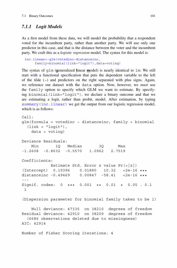
7.1 Binary Outcomes 101
7.1.1 Logit Models
As a first model from these data, we will model the probability that a respondentvoted for the incumbent party, rather than another party. We will use only onepredictor in this case, and that is the distance between the voter and the incumbentparty. We craft this as a logistic regression model. The syntax for this model is:
inc.linear<-glm(votedinc~distanceinc,family=binomial(link="logit"),data=voting)
The syntax of glm (generalized linear model) is nearly identical to lm: We stillstart with a functional specification that puts the dependent variable to the leftof the tilde (~) and predictors on the right separated with plus signs. Again,we reference our dataset with the data option. Now, however, we must usethe family option to specify which GLM we want to estimate. By specify-ing binomial(link="logit"), we declare a binary outcome and that weare estimating a logit, rather than probit, model. After estimation, by typingsummary(inc.linear) we get the output from our logistic regression model,which is as follows:
Call:glm(formula = votedinc ~ distanceinc, family = binomial
(link = "logit"),data = voting)
Deviance Residuals:Min 1Q Median 3Q Max
-1.2608 -0.8632 -0.5570 1.0962 2.7519
Coefficients:Estimate Std. Error z value Pr(>|z|)
(Intercept) 0.19396 0.01880 10.32 <2e-16 ***distanceinc -0.49469 0.00847 -58.41 <2e-16 ***---Signif. codes: 0 *** 0.001 ** 0.01 * 0.05 . 0.11
(Dispersion parameter for binomial family taken to be 1)
Null deviance: 47335 on 38210 degrees of freedomResidual deviance: 42910 on 38209 degrees of freedom
(6686 observations deleted due to missingness)AIC: 42914
Number of Fisher Scoring iterations: 4

102 7 Generalized Linear Models
Table 7.1 Logit model ofprobability of voting forincumbent party, 30cross-national elections
Predictor Estimate Std. error z value Pr(> jzj)Intercept 0.1940 0.0188 10.32 0.0000
Distance �0.4947 0.0085 �58.41 0.0000
Notes: N D 38;211. AIC D 42;914. 69 % correctlypredicted. Data from Singh (2014a)
The printout looks similar to the printout of the linear model we estimated inChap. 6.1 A more formal presentation of our results can be found in Table 7.1.2
Comparing these results to the linear model, however, a few differences areimportant to note. First, the coefficient estimates themselves are not as meaningfulas those of the linear model. A logit model transforms our outcome of interest, theprobability of voting for the incumbent party, because it is bounded between 0 and 1.The logit transform is worthwhile because it allows us to use a linear predictionframework, but it calls for an added step of effort for interpretation. (See Sect. 7.1.3for more on this.) A second difference in the output is that it reports z ratios insteadof t ratios: Just as before, these are computed around the null hypothesis that thecoefficient is zero, and the formula for the ratio uses the estimate and standarderror in the same way. Yet, we now need to assume these statistics follow a normaldistribution, rather than a t distribution.3 Third, different fit statistics are presented:deviance scores and the Akaike information criterion (AIC).4
In Table 7.1, we report the coefficients, standard errors, and inferential infor-mation. We also report the AIC, which is a good fit index and has the feature ofpenalizing for the number of parameters. Unlike R2 in linear regression, though,the AIC has no natural metric that gives an absolute sense of model fit. Rather, itworks better as a means of comparing models, with lower values indicating a betterpenalized fit. To include a measure of fit that does have a natural scale to it, we alsoreport what percentage of responses our model correctly predicts. To compute this,all we need to do is determine whether the model would predict a vote for theincumbent party and compare this to how the respondent actually voted. In R,we can roll our own computation:
1In this case, the coefficient estimates we obtain are similar to those reported by Singh (2014a).However, our standard errors are smaller (and hence z and p values are bigger) because Singhclusters the standard errors. This is a useful idea because the respondents are nested withinelections, though multilevel models (which Singh also reports) address this issue as well—seeSect. 8.1.2LATEX users can create a table similar to this quickly by typing: library(xtable);xtable(inc.linear).3An explanation of how the inferential properties of this model are derived can be found in Eliason(1993, pp. 26–27).4Deviance is calculated as �2 times the logged ratio of the fitted likelihood to the saturatedlikelihood. Formally, �2 log L1
L2, where L1 is the fitted likelihood and L2 is the saturated likelihood.
R reports two quantities: the null deviance computes this for an intercept-only model that alwayspredicts the modal value, and the residual deviance calculates this for the reported model.

7.1 Binary Outcomes 103
predicted<-as.numeric(predict.glm(inc.linear,type="response")>.5)
true<-voting$votedinc[voting$voted==1]correct<-as.numeric(predicted==true)100*table(correct)/sum(table(correct))
On the first line, we create a vector of the predictions from the model. Thecode uses the predict.glm command, which usefully can forecast from anymodel estimated with the glm command. By specifying type="response" weclarify that we want our predictions to be on the probability scale (instead of thedefault scale of latent utility). We then ask if each probability is greater than 0.5.By wrapping all of this in the as.numeric command, we count all probabilitiesabove 0.5 as predicted values of 1 (for the incumbent) and all that are less than 0.5as predicted values of 0 (against the incumbent). On the second line, we simplysubset the original vector of the outcome from the original data to those that votedand hence were included in the model. This subsetting step is essential because theglm command automatically deletes missing data from estimation. Hence, withoutsubsetting, our predicted and true values would not properly link together. On thethird line, we create a vector coded 1 if the predicted value matches the true value,and on the fourth line we create a table of this vector. The printout is:
correct0 1
30.99108 69.00892
Hence, we know that the model correctly predicts 69 % of the outcome values,which we report in Table 7.1.
As one more example of logistic regression, Singh (2014a) compares a modelwith linear ideological distances to one with squared ideological distances. To fitthis alternative model, we type:
inc.squared<-glm(votedinc~distanceincsq,family=binomial(link="logit"),data=voting)
summary(inc.squared)
The output of the summary command on the second line is:
Call:glm(formula = votedinc ~ distanceincsq, family = binomial(link = "logit"),
data = voting)
Deviance Residuals:Min 1Q Median 3Q Max
-1.1020 -0.9407 -0.5519 1.2547 3.6552
Coefficients:Estimate Std. Error z value Pr(>|z|)
(Intercept) -0.179971 0.014803 -12.16 <2e-16 ***

104 7 Generalized Linear Models
distanceincsq -0.101549 0.002075 -48.94 <2e-16 ***---Signif. codes: 0 *** 0.001 ** 0.01 * 0.05 .0.1 1
(Dispersion parameter for binomial family taken to be 1)
Null deviance: 47335 on 38210 degrees of freedomResidual deviance: 43087 on 38209 degrees of freedom
(6686 observations deleted due to missingness)AIC: 43091
Number of Fisher Scoring iterations:}5
With this second model we can see how the AIC can be useful: With a higher valueof 43,091 in the quadratic model, we conclude that the model with linear ideologicaldistance fits better with an AIC of 42,914. This corresponds to the original article’sconclusion that the linear form of the variable fits better.
7.1.2 Probit Models
Logit models have gained traction over the years for the sake of simplicity incomputation and interpretation. (For instance, logit models can be interpreted withodds ratios.) However, a key assumption of logit models is that the error term inthe latent variable model (or the latent utility) has a logistic distribution. We maybe more content to assume that the error term of our model is normally distributed,given the prevalence of this distribution in nature and in asymptotic results.5 Probitregression allows us to fit a model with a binary outcome variable with a normallydistributed error term in the latent variable model.
To show how this alternative model of a binary outcome works, we turn to amodel of the probability a survey respondent voted at all. Singh (2014a) modelsthis as a function of the ideological proximity to the nearest party weighted by thecompetitiveness of the election. The theory here is that individuals with a relativelyproximate alternative in a competitive election are more likely to find it worthwhileto vote. We fit this model as follows:
turnout.linear<-glm(voted~distanceweighted,family=binomial(link="probit"),data=voting)
summary(turnout.linear)
5Additionally, in advanced settings for which we need to develop a multivariate distribution formultiple outcome variables, the normal distribution is relatively easy to work with.

7.1 Binary Outcomes 105
The output of our summary command is:
Call:glm(formula = voted ~ distanceweighted, family = binomial(link = "probit"),
data = voting)
Deviance Residuals:Min 1Q Median 3Q Max
-1.9732 0.5550 0.5550 0.5776 0.6644
Coefficients:Estimate Std. Error z value Pr(>|z|)
(Intercept) 1.068134 0.009293 114.942 < 2e-16
***distanceweighted -0.055074 0.011724 -4.698 2.63e-06
***---Signif. codes: 0 *** 0.001 ** 0.01 * 0.05 .0.1 1
(Dispersion parameter for binomial family taken tobe 1)
Null deviance: 37788 on 44896 degrees of freedomResidual deviance: 37766 on 44895 degrees of freedomAIC: 37770
Number of Fisher Scoring iterations: 4
The layout of these probit model results look similar to the results of the logit model.Note, though, that changing the distribution of the latent error term to a normaldistribution changes the scale of the coefficients, so the values will be differentbetween logit and probit models. The substantive implications typically are similarbetween the models, so the user must decide which model works best in terms ofassumptions and interpretation for the data at hand.
7.1.3 Interpreting Logit and Probit Results
An important feature of GLMs is that the use of a link function makes thecoefficients more difficult to interpret. With a linear regression model, as estimatedin Chap. 6, we could simply interpret the coefficient in terms of change in theexpected value of the outcome itself, holding the other variables equal. With a GLM,though, the mean of the outcome has been transformed, and the coefficient speaksto change in the transformed mean. Hence, for analyses like logit and probit models,

106 7 Generalized Linear Models
we need to take additional steps in order to interpret the effect an input has on theoutcome of interest.
For a logistic regression model, the analyst can quickly calculate the odds ratiofor each coefficient simply by taking the exponential of the coefficient.6 Recall thatthe odds of an event is the ratio of the probability the event occurs to the probabilityit does not occur: p
1�p . The odds ratio tells us the multiplicative factor by which theodds will change for a unit increase in the predictor. Within R, if we want the oddsratio for our distance coefficient in Table 7.1, we simply type:
exp(inc.linear$coefficients[-1])
This syntax will take the exponential of every coefficient estimate from our model,no matter the number of covariates. The [-1] omits the intercept, for which anodds ratio would be meaningless. Having only one predictor, the printout in thiscase is:
distanceinc0.6097611
We need to be careful when interpreting the meaning of odds ratios. In this case,for a one point increase in distance from the incumbent party on the ideology scale,the odds that a respondent will vote for the incumbent party diminish by a factor of0.61. (With multiple predictors, we would need to add the ceteris paribus caveat.)If, instead of interpreting as a multiplicative factor, the analyst preferred to discusschange in percentage terms, type:
100*(exp(inc.linear$coefficients[-1])-1)
In this case a value of �39.02389 is returned. Hence, we can say: for a one pointincrease in distance from the incumbent party on the ideology scale, the odds that arespondent will vote for the incumbent party diminish by 39 %. Remember, though,that all of these statements relate specifically to odds, so in this case we are referringto a 39 % decrease in the ratio of the probability of voting for the incumbent to theprobability of voting for any other party.
An alternative interpretation that often is easier to explain in text is to reportpredicted probabilities from a model. For a logistic regression model, inputting thepredictions from the linear function (the latent utilities) into the logistic cumulativedistribution function produces the predicted probability that the outcome takes avalue of 1. A simple approach to intuitively illustrate the effect of a predictor isto plot the predicted probabilities at every value that a predictor can take, whichshows how the probability changes in a nonlinear way as the predictor changes.We proceed first by creating our predicted probabilities:
distances<-seq(0,10,by=.1)inputs<-cbind(1,distances)colnames(inputs)<-c("constant","distanceinc")inputs<-as.data.frame(inputs)
6This is because the logit link function is the log-odds, or logarithm of the odds of the event.
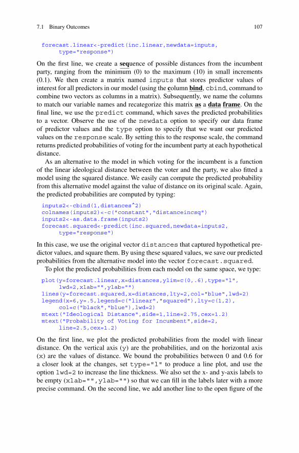
7.1 Binary Outcomes 107
forecast.linear<-predict(inc.linear,newdata=inputs,type="response")
On the first line, we create a sequence of possible distances from the incumbentparty, ranging from the minimum (0) to the maximum (10) in small increments(0.1). We then create a matrix named inputs that stores predictor values ofinterest for all predictors in our model (using the column bind, cbind, command tocombine two vectors as columns in a matrix). Subsequently, we name the columnsto match our variable names and recategorize this matrix as a data frame. On thefinal line, we use the predict command, which saves the predicted probabilitiesto a vector. Observe the use of the newdata option to specify our data frameof predictor values and the type option to specify that we want our predictedvalues on the response scale. By setting this to the response scale, the commandreturns predicted probabilities of voting for the incumbent party at each hypotheticaldistance.
As an alternative to the model in which voting for the incumbent is a functionof the linear ideological distance between the voter and the party, we also fitted amodel using the squared distance. We easily can compute the predicted probabilityfrom this alternative model against the value of distance on its original scale. Again,the predicted probabilities are computed by typing:
inputs2<-cbind(1,distances^2)colnames(inputs2)<-c("constant","distanceincsq")inputs2<-as.data.frame(inputs2)forecast.squared<-predict(inc.squared,newdata=inputs2,
type="response")
In this case, we use the original vector distances that captured hypothetical pre-dictor values, and square them. By using these squared values, we save our predictedprobabilities from the alternative model into the vector forecast.squared.
To plot the predicted probabilities from each model on the same space, we type:
plot(y=forecast.linear,x=distances,ylim=c(0,.6),type="l",lwd=2,xlab="",ylab="")
lines(y=forecast.squared,x=distances,lty=2,col="blue",lwd=2)legend(x=6,y=.5,legend=c("linear","squared"),lty=c(1,2),
col=c("black","blue"),lwd=2)mtext("Ideological Distance",side=1,line=2.75,cex=1.2)mtext("Probability of Voting for Incumbent",side=2,
line=2.5,cex=1.2)
On the first line, we plot the predicted probabilities from the model with lineardistance. On the vertical axis (y) are the probabilities, and on the horizontal axis(x) are the values of distance. We bound the probabilities between 0 and 0.6 fora closer look at the changes, set type="l" to produce a line plot, and use theoption lwd=2 to increase the line thickness. We also set the x- and y-axis labels tobe empty (xlab="",ylab="") so that we can fill in the labels later with a moreprecise command. On the second line, we add another line to the open figure of the

108 7 Generalized Linear Models
Fig. 7.1 Predictedprobability of voting for theincumbent party as a functionof ideological distance fromthe incumbents, based on alinear and a quadraticfunctional form
0 2 4 6 8 10
linearsquared
Ideological Distance
Pro
babi
lity
of V
otin
g fo
r In
cum
bent
0.0
0.1
0.2
0.3
0.4
0.5
0.6
predicted probabilities from the model with squared distance. This time, we colorthe line blue and make it dashed (lty=2) to distinguish it from the other model’spredicted probabilities. On the third line, we add a legend to the plot, located at thecoordinates where x=6 and y=0.5, that distinguishes the lines based on the linearand squared distances. Finally, on the last two lines we add axis labels using themtext command: The side option lets us declare which axis we are writing on,the line command determines how far away from the axis the label is printed, andthe cex command allows us to expand the font size (to 120 % in this case). Thefull results are presented in Fig. 7.1. As the figure shows, the model with squareddistance is more responsive at middle values, with a flatter response at extremes.Hence, Singh’s (2014a) conclusion that linear distance fits better has substantiveimplications for voter behavior.
As one final example of reporting predicted probabilities, we turn to an examplefrom the probit model we estimated of turnout. Predicted probabilities are computedin a similar way for probit models, except that the linear predictions (or utilities) arenow input into a normal cumulative distribution function. In this example, we willadd to our presentation of predicted probabilities by including confidence intervalsaround our predictions, which convey to the reader the level of uncertainty in ourforecast. We begin as we did in the last example, by creating a data frame ofhypothetical data values and producing predicted probabilities with them:
wght.dist<-seq(0,4,by=.1)inputs.3<-cbind(1,wght.dist)colnames(inputs.3)<-c("constant","distanceweighted")inputs.3<-as.data.frame(inputs.3)forecast.probit<-predict(turnout.linear,newdata=inputs.3,
type="link",se.fit=TRUE)

7.1 Binary Outcomes 109
In this case, weighted ideological distance from the nearest ideological party is ourone predictor. This predictor ranges from approximately 0–4, so we create a vectorspanning those values. On the last line of the above code, we have changed twofeatures: First, we have specified type="link". This means that our predictionsare now linear predictions of the latent utility, and not the probabilities in whichwe are interested. (This will be corrected in a moment.) Second, we have addedthe option se.fit=TRUE, which provides us with a standard error of each linearprediction. Our output object, forecast.probit now contains both the linearforecasts and the standard errors.
The reason we saved the linear utilities instead of the probabilities is that doingso will make it easier for us to compute confidence intervals that stay within theprobability limits of 0 and 1. To do this, we first compute the confidence intervalsof the linear predictions. For the 95 % confidence level, we type:
lower.ci<-forecast.probit$fit-1.95996399*forecast.probit$se.fitupper.ci<-forecast.probit$fit+1.95996399*forecast.probit$se.fit
Notice that by calling forecast.probit$fit we obtain the linear predictionsof utilities, and by calling forecast.probit$se.fit we call the standarderrors of our forecast. 1.95996399 is the two-tailed 95 % critical value from anormal distribution. Now that we have vectors of the lower and upper bounds ofthe confidence interval, we can insert these into the normal cumulative distributionfunction to put the bounds on the predicted probability scale.
We can now plot the predicted probabilities with confidence intervals as follows:
plot(y=pnorm(forecast.probit$fit),x=wght.dist,ylim=c(.7,.9),type="l",lwd=2,xlab="Weighted Ideological Distance",ylab="Probability of Turnout")
lines(y=pnorm(lower.ci),x=wght.dist,lty=3,col="red",lwd=2)lines(y=pnorm(upper.ci),x=wght.dist,lty=3,col="red",lwd=2)
In the first line, we plot the predicted probabilities themselves. To obtain the proba-bilities for the vertical axis, we type y=pnorm(forecast.probit$fit). Thepnorm function is the normal cumulative distribution function, so this convertsour linear utility predictions into actual probabilities. Meanwhile, x=wght.distplaces the possible values of weighted distance to the nearest party on the horizontalaxis. On the second line, we plot the lower bound of the 95 % confidence intervalof predicted probabilities. Here, pnorm(lower.ci) converts the confidenceinterval forecast onto the probability scale. Finally, we repeat the process on linethree to plot the upper bound of the confidence interval. The full output can be seenin Fig. 7.2. A noteworthy feature of this plot is that the confidence interval becomesnoticeably wide for the larger values of weighted distance. This is because the meanof the variable is low and there are few observations at these higher values.
The predicted probabilities in both of these cases were simple because theyincluded only one predictor. For any GLM, including a logit or probit model,predicted probabilities and their level of responsiveness depend on the value ofall covariates. Whenever a researcher has multiple predictors in a GLM model,

110 7 Generalized Linear Models
0 1 2 3 4
Weighted Ideological Distance
Pro
babi
lity
of T
urno
ut
0.70
0.75
0.80
0.85
0.90
Fig. 7.2 Predicted probability of turning out to vote as a function of weighted ideological distancefrom the nearest party, with 95 % confidence intervals
reasonable values of the control variables must be included in the forecasts. SeeSect. 7.3.3 for an example of using the predict function for a GLM that includesmultiple predictors.
7.2 Ordinal Outcomes
We now turn to ordinal outcome measures. Ordinal variables have multiple cate-gories as responses that can be ranked from lowest to highest, but other than therankings the numeric values have no inherent meaning. As an example of an ordinaloutcome variable, we again use survey data from the CSES, this time from Singh’s(2014b) study of satisfaction with democracy. Relative to the previous example,these data have a wider scope, including 66,908 respondents from 62 elections. Thevariables in this data set are as follows:
satisfaction: Respondent’s level of satisfaction with democracy. Ordinal scalecoded 1 (not at all satisfied), 2 (not very satisfied), 3 (fairly satisfied), or 4(very satisfied).
cntryyear: A character variable listing the country and year of the election.cntryyearnum: A numeric index identifying the country-year of the election.freedom: Freedom House scores for a country’s level of freedom. Scores range
from �5.5 (least free) to �1 (most free).gdpgrowth: Percentage growth in Gross Domestic Product (GDP).

7.2 Ordinal Outcomes 111
gdppercapPPP: GDP per capita, computed using purchasing price parity (PPP),chained to 2000 international dollars, in thousands of dollars.
CPI: Corruption Perceptions Index. Scores range from 0 (least corrupt) to 7.6(most corrupt).
efficacy: Respondent thinks that voting can make a difference. Ordinal scale from1 (disagree) to 5 (agree).
educ: Indicator coded 1 if the respondent graduated from college, 0 if not.abstained: Indicator coded 1 if the respondent abstained from voting, 0 if the
respondent voted.prez: Indicator coded 1 if the country has a presidential system, 0 if not.majoritarian_prez: Indicator coded 1 if the country has a majoritarian system, 0
if not.winner: Indicator coded 1 if the respondent voted for the winning party, 0 if not.voted_ID: Indicator coded 1 if the respondent voted for the party he or she
identifies with, 0 if not.voted_affect: Indicator coded 1 if the respondent voted for the party he or she
rated highest, 0 if not.voted_ideo: Indicator coded 1 if the respondent voted for the most similar party
on ideology, 0 if not.optimality: Vote optimality scale ranging from 0 to 3, coded by adding voted_ID,
voted_affect, and voted_ideo.winnerXvoted_ID: Interaction term between voting for the winner and voting by
party identification.winnerXvoted_affect: Interaction term between voting for the winner and voting
for the highest-rated party.winnerXvoted_ideo: Interaction term between voting for the winner and voting
by ideological similarity.winnerXoptimality: Interaction term between voting for the winner and the vote
optimality scale.
These data are also in Stata format, so if the foreign library is notalready loaded, it will need to be called. To load our data, download the fileSinghEJPR.dta from the Dataverse linked on page vii or the chapter contentlinked on page 97. Then type:
library(foreign)satisfaction<-read.dta("SinghEJPR.dta")
In this example, we wish to model each respondent’s level of satisfaction withdemocracy. This variable takes on the values 1, 2, 3, and 4, and we can only makestatements about which values reflect higher levels of satisfaction. In other words,we can say that a value of 4 (“very satisfied") reflects higher satisfaction than avalue of 3 (“fairly satisfied"), a value of 3 is more than 2 (“not very satisfied”),and therefore a value of 4 is higher than a value of 2. We cannot, however, say howmuch more satisfaction one value reflects relative to another, as the numbers have noinherent meaning other than providing a rank order of satisfaction. To do so would

112 7 Generalized Linear Models
require us to quantify adjectives such as “very” and “fairly.” Hence, an ordered logitor ordered probit model is going to be appropriate for this analysis.
As our first example, Singh (2014b, Table SM2) fits a model in which satisfactionin democracy is based on whether the respondent voted for the candidate mostideologically proximate, whether the candidate voted for the winner, and theinteraction between these two variables.7 The most important of these terms is theinteraction, as it tests the hypothesis that individuals who were on the winningside and voted for the most similar party ideologically will express the greatestsatisfaction.
Turning to specifics, for ordinal regression models we actually must use thespecial command polr (short for proportional odds logistic regression), which ispart of the MASS package. Most R distributions automatically install MASS, thoughwe still need to load it with the library command.8 In order to load the MASSpackage and then estimate an ordered logit model with these data, we would type:
library(MASS)satisfaction$satisfaction<-ordered(as.factor(
satisfaction$satisfaction))ideol.satisfaction<-polr(satisfaction~voted_ideo*winner+
abstained+educ+efficacy+majoritarian_prez+freedom+gdppercapPPP+gdpgrowth+CPI+prez,method="logistic",data=satisfaction)
summary(ideol.satisfaction)
Observe that we recode our dependent variable, satisfaction, using theas.factor command that was introduced in Sect. 2.4.2. We further embedthis within the ordered command to convey that the factor can be orderednumerically. We had to recode in this way because the model command polrrequires the outcome to be saved as a vector of class factor. Meanwhile, theright-hand side of the model resembles all other models we have estimated so farby separating variable names by plus signs. Notice that we use interactive notationwith voted_ideo*winner, in order to include both terms plus the product.9
All together, we have modeled satisfaction as a function of whether the votervoted for the most ideologically similar party, voted for the winner, an interactionterm between the two, and several other individual-level and country-level controlvariables. Within the command, the option method="logistic" specifies thatwe wish to estimate an ordered logit model rather than use another link function.At the end of the line, we specify our data option as usual to point to our data setof interest.
7This and the next example do not exactly replicate the original results, which also include randomeffects by country-year. Also, the next example illustrates ordered probit regression, instead of theordered logistic model from the original article. Both of the examples are based on models foundin the online supporting material at the European Journal of Political Research website.8If a user does need to install the package, install.packages("MASS") will do the job.9An equivalent specification would have been to include voted_ideo+winner+winnerXvoted_ideo as three separate terms from the data.
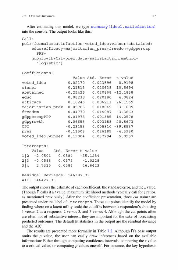
7.2 Ordinal Outcomes 113
After estimating this model, we type summary(ideol.satisfaction)into the console. The output looks like this:
Call:polr(formula=satisfaction~voted_ideo*winner+abstained+
educ+efficacy+majoritarian_prez+freedom+gdppercapPPP+
gdpgrowth+CPI+prez,data=satisfaction,method="logistic")
Coefficients:Value Std. Error t value
voted_ideo -0.02170 0.023596 -0.9198winner 0.21813 0.020638 10.5694abstained -0.25425 0.020868 -12.1838educ 0.08238 0.020180 4.0824efficacy 0.16246 0.006211 26.1569majoritarian_prez 0.05705 0.018049 3.1609freedom 0.04770 0.014087 3.3863gdppercapPPP 0.01975 0.001385 14.2578gdpgrowth 0.06653 0.003188 20.8673CPI -0.23153 0.005810 -39.8537prez -0.11503 0.026185 -4.3930voted_ideo:winner 0.19004 0.037294 5.0957
Intercepts:Value Std. Error t value
1|2 -2.0501 0.0584 -35.12842|3 -0.0588 0.0575 -1.02283|4 2.7315 0.0586 46.6423
Residual Deviance: 146397.33AIC: 146427.33
The output shows the estimate of each coefficient, the standard error, and the z value.(Though R calls it a t value, maximum likelihood methods typically call for z ratios,as mentioned previously.) After the coefficient presentation, three cut points arepresented under the label of Intercepts. These cut points identify the model byfinding where on a latent utility scale the cutoff is between a respondent’s choosing1 versus 2 as a response, 2 versus 3, and 3 versus 4. Although the cut points oftenare often not of substantive interest, they are important for the sake of forecastingpredicted outcomes. The default fit statistics in the output are the residual devianceand the AIC.
The results are presented more formally in Table 7.2. Although R’s base outputomits the p value, the user can easily draw inferences based on the availableinformation: Either through computing confidence intervals, comparing the z valueto a critical value, or computing p values oneself. For instance, the key hypothesis

114 7 Generalized Linear Models
Table 7.2 Ordered logit model of satisfaction with democracy, 62 cross-national elections
Predictor Estimate Std. error z value Pr(> jzj)Voted for proximate party �0:0217 0.0236 �0:9198 0.3577
Voted for winner 0:2181 0.0206 10:5694 0.0000
Voted proximate�winner 0:1900 0.0373 5:0957 0.0000
Abstained �0:2542 0.0209 �12:1838 0.0000
College graduate 0:0824 0.0202 4:0824 0.0000
Efficacy 0:1625 0.0062 26:1569 0.0000
Majoritarian system 0:0571 0.0180 3:1609 0.0016
Freedom 0:0477 0.0141 3:3863 0.0007
Economic development 0:0197 0.0014 14:2578 0.0000
Economic growth 0:0665 0.0032 20:8673 0.0000
Corruption �0:2315 0.0058 �39:8537 0.0000
Presidential system �0:1150 0.0262 �4:3930 0.0000
�1 �2:0501 0.0584 �35:1284 0.0000
�2 �0:0588 0.0575 �1:0228 0.3064
�3 2:7315 0.0586 46:6423 0.0000
Notes: N D 66;908. AIC D 146;427. Data from Singh (2014b)
here is for the interaction term to be positive. Hence, we can obtain our one-tailed pvalue by typing:
1-pnorm(5.0957)
R prints out 1.737275e-07, which in scientific notation means p D 0:00000017.Therefore, we will conclude with 99.9 % confidence that the coefficient on theinteraction term is discernibly greater than zero. In Table 7.2, we have opted toreport the two-tailed p values.10
A nice feature of using the logit link function, is that the results can be interpretedin terms of odds ratios. Odds ratios need to be computed and interpreted a bitdifferently for an ordinal model, though. See Long (1997, pp. 138–140) for a fullexplanation. For ordered logit models, we must exponentiate the negative value of acoefficient and interpret the odds of being in lower groups relative to higher groups.By way of example, the odds ratios for our coefficients from Table 7.2, along withthe percentage changes in odds, can be produced at once:
10Unfortunately the xtable command does not produce ready-made LATEX tables for results frompolr. By creating a matrix with the relevant results, though, LATEX users can produce a table fasterthan hand coding, though some revisions of the final product are necessary. Try the following:coef<-c(ideol.satisfaction$coefficients,ideol.satisfaction$zeta)se<-sqrt(diag(vcov(ideol.satisfaction)))z<-coef/sep<-2*(1-pnorm(abs(z)))xtable(cbind(coef,se,z,p),digits=4)

7.2 Ordinal Outcomes 115
exp(-ideol.satisfaction$coefficients)100*(exp(-ideol.satisfaction$coefficients)-1)
The resulting printout from the second line is:
voted_ideo winner abstained2.194186 -19.597657 28.949139
educ efficacy majoritarian_prez-7.908003 -14.994659 -5.545347freedom gdppercapPPP gdpgrowth
-4.658313 -1.955471 -6.436961CPI prez voted_ideo:winner
26.053177 12.190773 -17.307376
If we wanted to interpret the effect of efficacy, then, we could say for a one pointincrease on a five-point efficacy scale, the odds a respondent will report that they are“not at all satisfied” with democracy relative to any of the three higher categoriesdecrease by 15 %, ceteris paribus. Also, the odds that a respondent will report “notat all satisfied” or “not very satisfied” relative to the two higher categories alsodecrease by 15 %, all else equal. Further still, the odds that a respondent will reportone of the bottom three satisfaction levels relative to the highest category of “verysatisfied” diminish by 15 %, holding the other predictors constant. In general, then,we can interpret an odds ratio for an ordered logit as shaping the odds of all optionsbelow a threshold relative to all options above a threshold.
As a second example, we turn now to a model of voter satisfaction that focusesnot on the role of ideological proximity in vote choice, but instead on which party thevoter evaluated the most highly when asked to rate the parties. Again, the interactionbetween voting for the highest-rated party and also voting for the winning party isthe primary coefficient of interest. This time, we will also try a different link functionand estimate an ordered probit model instead of an ordered logit model. In this casewe will type:
affect.satisfaction<-polr(satisfaction~voted_affect*winner+abstained+educ+efficacy+majoritarian_prez+freedom+gdppercapPPP+gdpgrowth+CPI+prez,method="probit",data=satisfaction)
Besides changing one of the interacted variables, the only difference between thiscode and the prior command for the ordered logit command is the specification ofmethod="probit". This changes the scale of our coefficients somewhat, but thesubstantive implications of results are generally similar regardless of this choice.By typing summary(affect.satisfaction), we obtain the output:
Call:polr(formula = satisfaction ~ voted_affect * winner +abstained +
educ + efficacy + majoritarian_prez + freedom +gdppercapPPP +

116 7 Generalized Linear Models
gdpgrowth + CPI + prez, data = satisfaction, method= "probit")
Coefficients:Value Std. Error t value
voted_affect 0.03543 0.0158421 2.237winner 0.04531 0.0245471 1.846abstained -0.11307 0.0170080 -6.648educ 0.05168 0.0115189 4.487efficacy 0.09014 0.0035177 25.625majoritarian_prez 0.03359 0.0101787 3.300freedom 0.03648 0.0082013 4.448gdppercapPPP 0.01071 0.0007906 13.546gdpgrowth 0.04007 0.0018376 21.803CPI -0.12897 0.0033005 -39.075prez -0.03751 0.0147650 -2.540voted_affect:winner 0.14278 0.0267728 5.333
Intercepts:Value Std. Error t value
1|2 -1.1559 0.0342 -33.75152|3 -0.0326 0.0340 -0.95863|4 1.6041 0.0344 46.6565
Residual Deviance: 146698.25AIC: 146728.25
Once again, our hypothesis of interest is supported by the results, with a positiveand discernible effect on the interaction between voting for the winning party andvoting for the highest-rated party.
7.3 Event Counts
As a third type of GLM, we turn to models of event counts. Whenever our dependentvariable is the number of events that occurs within a defined period of time, thevariable will have the feature that it can never be negative and must take on adiscrete value (e.g., 0,1,2,3,4, . . . ). Count outcomes therefore tend to have a strongright skew and a discrete probability distribution such as the Poisson or negativebinomial distribution.
As an example of count data, we now return to Peake and Eshbaugh-Soha’s(2008) data that were previously discussed in Chap. 3. Recall that the outcomevariable in this case is the number of television news stories related to energy policyin a given month. (See Chap. 3 for additional details on the data.) The number ofnews stories in a month certainly is an event count. However, note that because

7.3 Event Counts 117
these are monthly data, they are time dependent, which is a feature we ignore at thistime. In Chap. 9 we revisit this issue and consider models that account for time. Fornow, though, this illustrates how we usually fit count models in R.
First, we load the data again:11
pres.energy<-read.csv("PESenergy.csv")
After viewing the descriptive statistics on our variables and visualizing the data aswe did in Chap. 3, we can now turn to fitting a model.
7.3.1 Poisson Regression
The simplest count model we can fit is a Poisson model. If we were to type:
energy.poisson<-glm(Energy~rmn1173+grf0175+grf575+jec477+jec1177+jec479+embargo+hostages+oilc+Approval+Unemploy,family=poisson(link=log),data=pres.energy)
This will fit a Poisson regression model in which TV coverage of energypolicy is a function of six terms for presidential speeches, an indicator forthe Arab oil embargo, an indicator for the Iran hostage crisis, the priceof oil, presidential approval, and the unemployment rate.12 Notice that thistime, we set family=poisson(link=log), declaring the distribution ofthe outcome as Poisson and specifying our log link function. If we typesummary(energy.poisson) into the console, R returns the following output:
Call:
glm(formula = Energy ~ rmn1173 + grf0175 + grf575 +
jec477 +
jec1177 + jec479 + embargo + hostages + oilc +
Approval +
Unemploy, family = poisson(link = log), data = pres.
energy)
Deviance Residuals:
Min 1Q Median 3Q Max
-8.383 -2.994 -1.054 1.536 11.399
Coefficients:
Estimate Std. Error z value Pr(>|z|)
(Intercept) 13.250093 0.329121 40.259 < 2e-16 ***rmn1173 0.694714 0.077009 9.021 < 2e-16 ***
11The footnote should read: "For users who do not have the file handy from Chapter 3, pleasedownload the file from the Dataverse linked on page vii or the chapter content linked on page 97.12Note that the presidential speech terms are coded 1 only in the month of the speech, and 0 in allother months. The terms for the oil embargo and hostage crisis were coded 1 while these eventswere ongoing and 0 otherwise.

118 7 Generalized Linear Models
grf0175 0.468294 0.096169 4.870 1.12e-06 ***grf575 -0.130568 0.162191 -0.805 0.420806
jec477 1.108520 0.122211 9.071 < 2e-16 ***jec1177 0.576779 0.155511 3.709 0.000208 ***jec479 1.076455 0.095066 11.323 < 2e-16 ***embargo 0.937796 0.051110 18.349 < 2e-16 ***hostages -0.094507 0.046166 -2.047 0.040647 *oilc -0.213498 0.008052 -26.515 < 2e-16 ***Approval -0.034096 0.001386 -24.599 < 2e-16 ***Unemploy -0.090204 0.009678 -9.321 < 2e-16 ***---
Signif. codes: 0 *** 0.001 ** 0.01 * 0.05 . 0.1 1
(Dispersion parameter for poisson family taken to be 1)
Null deviance: 6009.0 on 179 degrees of freedom
Residual deviance: 2598.8 on 168 degrees of freedom
AIC: 3488.3
Number of Fisher Scoring iterations: 5
The format of the output—coefficient estimates, standard errors, z, and p—should be very familiar by now, as are the deviance and AIC scores. In this casethe link function is simply a logarithm, so although the coefficients themselvesare not very meaningful, interpretation is still simple. As one option, if we take theexponential of a coefficient, this offers us a count ratio, which allows us to deducethe percentage change in the expected count for a change in the input variable. Forinstance, if we wanted to interpret the effect of presidential approval, we could type:
exp(-.034096)
Here, we simply inserted the estimated coefficient from the printed output. Theresult gives us a count ratio of 0.9664787. We could interpret this as meaning fora percentage point increase in the president’s approval rating, coverage of energypolicy diminishes by 3.4 % on average and holding all other predictors equal. Asa quick way to get the count ratio and percentage change for every coefficient, wecould type:
exp(energy.poisson$coefficients[-1])100*(exp(energy.poisson$coefficients[-1])-1)
In both lines the [-1] index for the coefficient vector throws away the interceptterm, for which we do not want a count ratio. The printout from the second linereads:
rmn1173 grf0175 grf575 jec477 jec1177100.313518 59.726654 -12.240295 202.987027 78.029428
jec479 embargo hostages oilc Approval193.425875 155.434606 -9.017887 -19.224639 -3.352127
Unemploy-8.625516

7.3 Event Counts 119
From this list, we can simply read-off the percentage changes for a one-unit increasein the input, holding the other inputs equal. For a graphical means of interpretation,see Sect. 7.3.3.
7.3.2 Negative Binomial Regression
An intriguing feature of the Poisson distribution is that the variance is the same asthe mean. Hence, when we model the logarithm of the mean, our model is simul-taneously modeling the variance. Often, however, we find that the variance of ourcount variable is wider than we would expect given the covariates—a phenomenoncalled overdispersion. Negative binomial regression offers a solution to this problemby estimating an extra dispersion parameter that allows the conditional variance todiffer from the conditional mean.
In R, negative binomial regression models actually require a special commandfrom the MASS library called glm.nb. If the MASS library is not loaded, be sureto type library(MASS) first. Then, we can fit the negative binomial model bytyping:
energy.nb<-glm.nb(Energy~rmn1173+grf0175+grf575+jec477+jec1177+jec479+embargo+hostages+oilc+Approval+Unemploy,data=pres.energy)
Notice that the syntax is similar to the glm command, but there is no familyoption since the command itself specifies that. By typing summary(energy.nb)the following results print:
Call:glm.nb(formula = Energy ~ rmn1173 + grf0175 + grf575 +
jec477 +jec1177 + jec479 + embargo + hostages + oilc +Approval +
Unemploy, data = pres.energy, init.theta =2.149960724, link = log)
Deviance Residuals:Min 1Q Median 3Q Max
-2.7702 -0.9635 -0.2624 0.3569 2.2034
Coefficients:Estimate Std. Error z value Pr(>|z|)
(Intercept) 15.299318 1.291013 11.851 < 2e-16 ***rmn1173 0.722292 0.752005 0.960 0.33681grf0175 0.288242 0.700429 0.412 0.68069grf575 -0.227584 0.707969 -0.321 0.74786jec477 0.965964 0.703611 1.373 0.16979

120 7 Generalized Linear Models
jec1177 0.573210 0.702534 0.816 0.41455jec479 1.141528 0.694927 1.643 0.10045embargo 1.140854 0.350077 3.259 0.00112 **hostages 0.089438 0.197520 0.453 0.65069oilc -0.276592 0.030104 -9.188 < 2e-16 ***Approval -0.032082 0.005796 -5.536 3.1e-08 ***Unemploy -0.077013 0.037630 -2.047 0.04070 *---Signif. codes: 0 *** 0.001 ** 0.01 * 0.05 . 0.1 1
(Dispersion parameter for Negative Binomial(2.15) familytaken
to be 1)
Null deviance: 393.02 on 179 degrees of freedomResidual deviance: 194.74 on 168 degrees of freedomAIC: 1526.4
Number of Fisher Scoring iterations: 1
Theta: 2.150Std. Err.: 0.242
2 x log-likelihood: -1500.427
The coefficients reported in this output can be interpreted in the same way thatcoefficients from a Poisson model are interpreted because both model the logarithmof the mean. The key addition, reported at the end of the printout, is the dispersionparameter . In this case, our estimate is O D 2:15, and with a standard errorof 0.242 the result is discernible. This indicates that overdispersion is present inthis model. In fact, many of the inferences drawn vary between the Poisson andnegative binomial models. The two models are presented side by side in Table 7.3.As the results show, many of the discernible results from the Poisson model are notdiscernible in the negative binomial model. Further, the AIC is substantially lowerfor the negative binomial model, indicating a better fit even when penalizing for theextra overdispersion parameter.

7.3 Event Counts 121
7.3.3 Plotting Predicted Counts
While count ratios are certainly a simple way to interpret coefficients from countmodels, we have the option of graphing our results as well. In this case, we modelthe logarithm of our mean parameter, so we must exponentiate our linear predictionto predict the expected count given our covariates. As with logit and probit models,for count outcomes the predict command makes forecasting easy.
Suppose we wanted to plot the effect of presidential approval on the number ofTV news stories on energy, based on the two models of Table 7.3. This situationcontrasts a bit from the graphs we created in Sect. 7.1.3. In all of the logit and probitexamples, we only had one predictor. By contrast, in this case we have severalother predictors, so we have to set those to plausible alternative values. For thisexample, we will set the value of all dummy variable predictors to their modal valueof zero, while the price of oil and unemployment are set to their mean. If we failto insert reasonable values for the covariates, the predicted counts will not resemblethe actual mean and the size of the effect will not be reasonable.13 In this example,the way in which we use the predict command to forecast average counts withmultiple predictors can be used in exactly the same way for a logit or probit modelto forecast predicted probabilities with multiple predictors.
Table 7.3 Two count models of monthly TV new stories on energy policy, 1969–1983
Poisson Negative binomial
Parameter Estimate Std. error Pr(> jzj) Estimate Std. error Pr(> jzj)Intercept 13.2501 0.3291 0.0000 15.2993 1.2910 0.0000
Nixon 11/73 0.6947 0.0770 0.0000 0.7223 0.7520 0.3368
Ford 1/75 0.4683 0.0962 0.0000 0.2882 0.7004 0.6807
Ford 5/75 �0.1306 0.1622 0.4208 �0.2276 0.7080 0.7479
Carter 4/77 1.1085 0.1222 0.0000 0.9660 0.7036 0.1698
Carter 11/77 0.5768 0.1555 0.0002 0.5732 0.7025 0.4145
Carter 4/79 1.0765 0.0951 0.0000 1.1415 0.6949 0.1005
Arab oil embargo 0.9378 0.0511 0.0000 1.1409 0.3501 0.0011
Iran hostage crisis �0.0945 0.0462 0.0406 0.0894 0.1975 0.6507
Price of oil �0.2135 0.0081 0.0000 �0.2766 0.0301 0.0000
Presidential approval �0.0341 0.0014 0.0000 �0.0321 0.0058 0.0000
Unemployment �0.0902 0.0097 0.0000 �0.0770 0.0376 0.0407
— 2.1500 0.2419 0.0000
AIC 3488.2830 1526.4272
Notes: N D 180. Data from Peake and Eshbaugh-Soha (2008)
13Besides this approach of making predictions using central values of control variables, Hanmerand Kalkan (2013) make the case that forecasting outcomes based on the observed values of controlvariables in the data set is preferable. Readers are encouraged to consult their article for furtheradvice on this issue.

122 7 Generalized Linear Models
Turning to specifics, in our data the variable approve ranges from 24%approval to 72.3%. Thus, we construct a vector that includes the full range ofapproval as well as plausible values of all of the other predictors:
approval<-seq(24,72.3,by=.1)inputs.4<-cbind(1,0,0,0,0,0,0,0,0,mean(pres.energy$oilc),
approval,mean(pres.energy$Unemploy))colnames(inputs.4)<-c("constant","rmn1173","grf0175",
"grf575","jec477","jec1177","jec479","embargo","hostages","oilc","Approval","Unemploy")
inputs.4<-as.data.frame(inputs.4)
The first line above creates the vector of hypothetical values of our predictor ofinterest. The second line creates a matrix of hypothetical data values—setting theindicator variables to zero, the continuous variables to their means, and approvalto its range of hypothetical values. The third line names the columns of the matrixafter the variables in our model. On the last line, the matrix of predictor values isconverted to a data frame.
Once we have the data frame of predictors in place, we can use the predictcommand to forecast the expected counts for the Poisson and negative binomialmodels:
forecast.poisson<-predict(energy.poisson,newdata=inputs.4,type="response")
forecast.nb<-predict(energy.nb,newdata=inputs.4,type="response")
These two lines only differ in the model from which they draw coefficient estimatesfor the forecast.14 In both cases, we specify type="response" to obtainpredictions on the count scale.
To graph our forecasts from each model, we can type:
plot(y=forecast.poisson,x=approval,type="l",lwd=2,ylim=c(0,60),xlab="Presidential Approval",ylab="Predicted Count of Energy Policy Stories")
lines(y=forecast.nb,x=approval,lty=2,col="blue",lwd=2)legend(x=50,y=50,legend=c("Poisson","Negative Binomial"),
lty=c(1,2),col=c("black","blue"),lwd=2)
The first line plots the Poisson predictions as a line with the type="l" option.The second line adds the negative binomial predictions, coloring the line blueand dashing it with lty=2. Finally, the legend command allows us to quicklydistinguish which line represents which model. The full output is presented inFig. 7.3. The predictions from the two models are similar and show a similarnegative effect of approval. The negative binomial model has a slightly lowerforecast at low values of approval and a slightly shallower effect of approval, suchthat the predicted counts overlap at high values of approval.
14As a side note, by using R’s matrix algebra commands, described furtherin Chap. 10, the user can compute predicted counts easily with alternatesyntax. For instance, for the negative binomial model, we could have typed:forecast.nb<-exp(as.matrix(inputs.4)%*%energy.nb$coefficients).

7.4 Practice Problems 123
30 40 50 60 70
010
2030
4050
60
Presidential Approval
Pre
dict
ed C
ount
of E
nerg
y P
olic
y S
torie
sPoissonNegative Binomial
Fig. 7.3 Predicted count of energy policy stories on TV news as a function of presidentialapproval, holding continuous predictors at their mean and nominal predictors at their mode.Predictions based on Poisson and negative binomial model results
After the first seven chapters of this volume, users should now be able to performmost of the basic tasks that statistical software is designed to do: manage data,compute simple statistics, and estimate common models. In the remaining fourchapters of this book, we now turn to the unique features of R that allow theuser greater flexibility to apply advanced methods with packages developed byother users and tools for programming in R.
7.4 Practice Problems
1. Logistic regression: Load the foreign library, and download a subsetof Singh’s (2015) cross-national survey data on voter turnout, the filestdSingh.dta, available from the Dataverse listed on page vii or thechapter content listed on page 97. The outcome variable is whether the surveyrespondent voted (voted). A key predictor, with which several variables areinteracted, is the degree to which a citizen is subject to mandatory voting rules.This is measured with a scale of how severe the compulsory voting rules are(severity). Five predictors should be interacted with severity: age (age), politicalknowledge (polinfrel), income (income), efficacy (efficacy), and partisanship(partyID). Five more predictors should be included only for additive effects:district magnitude (dist_magnitude), number of parties (enep), victory margin

124 7 Generalized Linear Models
(vicmarg_dist), parliamentary system (parliamentary), and per capita GDP(development). All of the predictor variables have been standardized.
a. Estimate a logistic regression model with these data, including the fiveinteraction terms.
b. What is the odds ratio for number of parties? How would you interpret thisterm?
c. Plot the effect of per capita GDP on the probability of turning out. Holdall predictors other than development at their mean. Hint: Build on thecode starting on page 107. If you used R’s interaction notation (e.g., ifage*severity is a term in the model), then when you create a new datasetof predictor values, you need only define your values for the original variables,and not for the products. In other words, you would need a column for age,for severity, and for any other predictors, but not for age � severity.
d. Bonus: Plot the effect of age on probability of turnout for three circumstances:When severity of compulsory voting rules is at its minimum, at its mean, andat its maximum. Hold all other predictors besides age and severity at theirmean. Your final result should show three different predicted probability lines.
2. Ordered logit: The practice problems from Chapter 2 introduced Hanmer andKalkan’s (2013) subset of the 2004 American National Election Study. If youdo not have these data already, the file hanmerKalkanANES.dta can bedownloaded from the Dataverse linked on page vii or from the chapter contentlinked on page 97. Load the foreign library and open these data. (Again,be sure to specify the convert.factors=F option.) Consider two outcomevariables: retrospective economic evaluations (retecon, taking on ordinal valuescoded �1, �0.5, 0, 0.5, and 1) and assessment of George W. Bush’s handlingof the war in Iraq (bushiraq, taking on ordinal values coded 0, 0.33, 0.67,and 1). There are seven predictor variables: partisanship on a seven-point scale(partyid), ideology on a seven-point scale (ideol7b), an indicator of whether therespondent is white (white), an indicator of whether the respondent is female(female), age of the respondent (age), level of education on a seven-point scale(educ1_7), and income on a 23-point scale (income).
a. Estimate an ordered logistic model of retrospective economic evaluations as afunction of the seven predictors.
b. What is the odds ratio on the coefficient for female? How would you interpretthis term?
c. Estimate an ordered logistic model of evaluation of Bush’s handling of thewar in Iraq as a function of the seven predictors.
d. What is the odds ratio on the coefficient for the seven-point partisanship scale?How would you interpret this term?
e. Bonus: The results of a model are biased if there is reciprocal causation,meaning that one of the independent variables not only influences thedependent variable, but also the dependent variable influences the independent
7.4 Practice Problems 125
variable. Suppose you were worried about reciprocal causation bias in themodel of retrospective economic evaluations. Which independent variable orvariables would be most suspect to this criticism?
3. Count model: In the practice problems from Chapters 3 and 4, we introducedPeake and Eshbaugh-Soha’s (2008) analysis of drug policy coverage. If youdo not have their data from before, download drugCoverage.csv fromthe Dataverse linked on page vii or the chapter content linked on page 97.The outcome variable is news coverage of drugs (drugsmedia), and the fourinputs are an indicator for a speech on drugs that Ronald Reagan gave inSeptember 1986 (rwr86), an indicator for a speech George H.W. Bush gave inSeptember 1989 (ghwb89), the president’s approval rating (approval), and theunemployment rate (unemploy).15
a. Estimate a Poisson regression model of drug policy coverage as a function ofthe four predictors.
b. Estimate a negative binomial regression model of drug policy coverage as afunction of the four predictors. Based on your models’ results, which modelis more appropriate, Poisson or negative binomial? Why?
c. Compute the count ratio for the presidential approval predictor for eachmodel. How would you interpret each quantity?
d. Plot the predicted counts from each model contingent on the unemploymentlevel, ranging from the minimum to maximum observed values. Hold thetwo presidential speech variables at zero, and hold presidential approvalat its mean. Based on this figure, what can you say about the effect ofunemployment in each model?
15Just as in the example from the chapter, these are time series data, so methods from Chap. 9 aremore appropriate.

Chapter 8Using Packages to Apply Advanced Models
In the first seven chapters of this book, we have treated R like a traditional statisticalsoftware program and reviewed how it can perform data management, report simplestatistics, and estimate a variety of regression models. In the remainder of this book,though, we turn to the added flexibility that R offers—both in terms of programmingcapacity that is available for the user as well as providing additional applied toolsthrough packages. In this chapter, we focus on how loading additional batches ofcode from user-written packages can add functionality that many software programswill not allow. Although we have used packages for a variety of purposes in theprevious seven chapters (including car, gmodels, and lattice, to name afew), here we will highlight packages that enable unique methods. While the CRANwebsite lists numerous packages that users may install at any given time, we willfocus on four particular packages to illustrate the kinds of functionality that can beadded.
The first package we will discuss, lme4, allows users to estimate multilevelmodels, thereby offering an extension to the regression models discussed in Chaps. 6and 7 (Bates et al. 2014). The other three were all developed specifically by PoliticalScientists to address data analytic problems that they encountered in their research:MCMCpack allows users to estimate a variety of models in a Bayesian frameworkusing Markov chain Monte Carlo (MCMC) (Martin et al. 2011). cem allows the userto conduct coarsened exact matching—a method for causal inference with field data(Iacus et al. 2009, 2011). Lastly, wnominate allows the user to scale choice data,such as legislative roll call data, to estimate ideological ideal points of legislatorsor respondents (Poole and Rosenthal 1997; Poole et al. 2011). The following foursections will consider each package separately, so each section will introduce itsdata example in turn. These sections are designed to offer a brief overview of the
Electronic supplementary material: The online version of this chapter(doi: 10.1007/978-3-319-23446-5_8) contains supplementary material, which is available toauthorized users.
© Springer International Publishing Switzerland 2015J.E. Monogan III, Political Analysis Using R, Use R!,DOI 10.1007/978-3-319-23446-5_8
127
128 8 Using Packages to Apply Advanced Models
kinds of capacities R packages offer, though some readers may be unfamiliar withthe background behind some of these methods. The interested reader is encouragedto consult with some of the cited resources to learn more about the theory behindthese methods.
8.1 Multilevel Models with lme4
Having discussed linear models in Chap. 6 and several examples of generalizedlinear models in Chap. 7, we now turn to an extension of these kinds of models:multilevel models. Multilevel models, or hierarchical models, are appropriatewhenever data of interest have either a nested or longitudinal structure. A nestedstructure occurs when observations can be thought of as being within or part ofan upper-level unit: A common policy example is to study learning outcomes forstudents, but the students are nested within classrooms. In such a case, the researcherwould need to account for the fact that the students in the sample are not independentof each other, but are likely to be similar if in the same classroom. Similarly,whenever a researcher studies individuals that have repeated observations over time,it is reasonable to think of the time-referenced observations as being embeddedwithin the individual’s observations. For example, in the LaLonde (1986) data firstintroduced in Chap. 4, the income of participants in his study are observed in 1974,1975, and 1978. Some policy analyses might opt to consider the three temporalobservations for each individual as being nested within each individual’s case.1
More comprehensive explanations of multilevel models can be found in Scott et al.(2013) and Gelman and Hill (2007). We proceed by extending two of our priorexamples to illustrate a multilevel linear model and a multilevel logit model.
8.1.1 Multilevel Linear Regression
In this example, we return to our example from Chap. 6 on the number of hoursteachers spend in the classroom teaching evolution. Originally, we fitted a linearmodel using ordinary least squares (OLS) as our estimator. However, Berkman andPlutzer (2010) make the point that teachers in the same state are likely to sharesimilar features. These features could be similarities in training, in the local culture,or in state law. To account for these unobserved similarities, we can think of teachersas being nested within states. For this reason, we will add a random effect for eachstate. Random effects account for intraclass correlation, or error correlation among
1Note that this multilevel approach to panel data is most sensible for short panels such as thesewhere there are many individuals relative to the number of time points. For long panels in whichthere are many time points relative to the number of individuals, more appropriate models aredescribed as pooled time series cross-section methods. For more on the study of short panels, seeMonogan (2011) and Fitzmaurice et al. (2004).

8.1 Multilevel Models with lme4 129
observations within the same group. In the presence of intraclass correlation, OLSestimates are inefficient because the disturbance terms are not independent, so arandom effects model accounts for this problem.
First, we reload the data from the National Survey of High School BiologyTeachers as follows:2
rm(list=ls())library(foreign)evolution<-read.dta("BPchap7.dta")evolution$female[evolution$female==9]<-NAevolution<-subset(evolution,!is.na(female))
Recall that we had a handful of observations of female that needed to be recodedas missing. As before, we subset our data to omit these missing observations.
In order to fit a multilevel model, there are actually a few commands available.We will opt to use a command from the lme4 (linear mixed effect) library.3 On ourfirst use, we will install the package, and then on every use we will load the library:
install.packages("lme4")library(lme4)
Once we have loaded the library, we fit our multilevel linear model using the lmer(linear mixed effects regression) command:
hours.ml<-lmer(hrs_allev~phase1+senior_c+ph_senior+notest_p+ph_notest_p+female+biocred3+degr3+evol_course+certified+idsci_trans+confident+(1|st_fip),data=evolution)
The syntax to the lmer command is nearly identical to the code we used whenfitting a model with OLS using lm. In fact, the only attribute we added is theadditional term (1|st_fip) on the right-hand side of the model. This adds arandom intercept by state. On any occasion for which we wish to include a randomeffect, in parentheses we place the term for which to include the effect followed by avertical pipe and the variable that identifies the upper-level units. So in this case wewanted a random intercept (hence the use of 1), and we wanted these to be assignedby state (hence the use of st_fip).
We obtain our results by typing:
summary(hours.ml)
In our result output, R prints the correlation between all of the fixed effects, orestimated regression parameters. This part of the printout is omitted below:
Linear mixed model fit by REML [’lmerMod’]Formula:hrs_allev~phase1+senior_c+ph_senior+notest_p+ph_notest_p+
2If you do not have these data from before, you can download the file BPchap7.dta from theDataverse on page vii or the chapter content on page 125.3See also the nlme library, which was a predecessor to lme4.

130 8 Using Packages to Apply Advanced Models
female+biocred3+degr3+evol_course+certified+idsci_trans+
confident+(1|st_fip)Data: evolution
REML criterion at convergence: 5940
Scaled residuals:Min 1Q Median 3Q Max
-2.3478 -0.7142 -0.1754 0.5566 3.8846
Random effects:Groups Name Variance Std.Dev.st_fip (Intercept) 3.089 1.758Residual 67.873 8.239Number of obs: 841, groups: st_fip, 49
Fixed effects:Estimate Std. Error t value
(Intercept) 10.5676 1.2138 8.706phase1 0.7577 0.4431 1.710senior_c -0.5291 0.3098 -1.708ph_senior -0.5273 0.2699 -1.953notest_p 0.1134 0.7490 0.151ph_notest_p -0.5274 0.6598 -0.799female -0.9702 0.6032 -1.608biocred3 0.5157 0.5044 1.022degr3 -0.4434 0.3887 -1.141evol_course 2.3894 0.6270 3.811certified -0.5335 0.7188 -0.742idsci_trans 1.7277 1.1161 1.548confident 2.6739 0.4468 5.984
The output first prints a variety of fit statistics: AIC, BIC, log-likelihood, deviance,and restricted maximum likelihood deviance. Second, it prints the variance andstandard deviation of the random effects. In this case, the variance for the st_fipterm is the variance of our state-level random effects. The residual variancecorresponds to the error variance of regression that we would normally compute forour residuals. Last, the fixed effects that are reported are synonymous with linearregression coefficients that we normally are interested in, albeit now our estimateshave accounted for the intraclass correlation among teachers within the same state.Table 8.1 compares our OLS and multilevel estimates side-by-side. As can be seen,the multilevel model now divides the unexplained variance into two components(state and individual-level), and coefficient estimates have changed somewhat.

8.1 Multilevel Models with lme4 131
Table 8.1 Two models of hours of class time spent teaching evolution by high school biologyteachers
OLS Multilevel
Parameter Estimate Std. error Pr(> jzj) Estimate Std. error Pr(> jzj)Intercept 10.2313 1.1905 0.0000 10.5675 1.2138 0.0000
Standards index 2007 0.6285 0.3331 0.0596 0.7576 0.4431 0.0873
Seniority (centered) �0.5813 0.3130 0.0636 �0.5291 0.3098 0.0876
Standards � seniority �0.5112 0.2717 0.0603 �0.5273 0.2699 0.0508
Believes there is no test 0.4852 0.7222 0.5019 0.1135 0.7490 0.8795
Standards � believes no test �0.5362 0.6233 0.3899 �0.5273 0.6598 0.4241
Teacher is female �1.3546 0.6016 0.0246 �0.9703 0.6032 0.1077
Credits earned in biology (0–2) 0.5559 0.5072 0.2734 0.5157 0.5044 0.3067
Science degrees (0–2) �0.4003 0.3922 0.3077 �0.4434 0.3887 0.2540
Completed evolution class 2.5108 0.6300 0.0001 2.3894 0.6270 0.0001
Has normal certification �0.4446 0.7212 0.5377 �0.5335 0.7188 0.4580
Identifies as scientist 1.8549 1.1255 0.0997 1.7277 1.1161 0.1216
Self- rated expertise (�1 to +2) 2.6262 0.4501 0.0000 2.6738 0.4468 0.0000
State-level variance — 3.0892
Individual-level variance 69.5046 67.8732
Notes: N D 841. Data from Berkman and Plutzer (2010)
8.1.2 Multilevel Logistic Regression
While somewhat more complex, the logic of multilevel modeling can also be appliedwhen studying limited dependent variables. There are two broad approaches toextending GLMs into a multilevel framework: marginal models, which have apopulation-averaged interpretation, and generalized linear mixed models (GLMMs),which have an individual-level interpretation (Laird and Fitzmaurice 2013, pp. 149–156). While readers are encouraged to read further on the kinds of models available,their estimation, and their interpretation, for now we focus on the process ofestimating a GLMM.
In this example, we return to our example from Sect. 7.1.1 from the last chapter,on whether a survey respondent reported voting for the incumbent party as afunction of the ideological distance from the party. As Singh (2014a) observes,voters making their choice in the same country-year are going to face many featuresof the choice that are unique to that election. Hence, intraclass correlation amongvoters within the same election is likely. Further, the effect of ideology itself may bestronger in some elections than it is in others: Multilevel methods including GLMMsallow us to evaluate whether there is variation in the effect of a predictor acrossgroups, which is a feature that we will use.

132 8 Using Packages to Apply Advanced Models
Turning to the specifics of code, if the lme4 library is not loaded, we need thatagain. Also, if the data from are not loaded, then we need to load the foreignlibrary and the data set itself. All of this is accomplished as follows:4
library(lme4)library(foreign)voting<-read.dta("SinghJTP.dta")
Building on the model from Table 7.1, we first simply add a random intercept toour model. The syntax for estimating the model and printing the results is:
inc.linear.ml<-glmer(votedinc~distanceinc+(1|cntryyear),family=binomial(link="logit"),data=voting)
summary(inc.linear.ml)
Notice that we now use the glmer command (generalized linear mixed effectsregression). By using the family option, we can use any of the common linkfunctions available for the glm command. A glance at the output shows that, inaddition to the traditional fixed effects that reflect logistic regression coefficients,we also are presented with the variance of the random intercept for country and yearof the election:
Generalized linear mixed model fit by the Laplaceapproximation
Formula: votedinc ~ distanceinc + (1 | cntryyear)Data: voting
AIC BIC logLik deviance41998.96 42024.62 -20996.48 41992.96
Random effects:Groups Name Variance Std.Dev.cntryyear (Intercept) 0.20663 0.45457
Number of obs: 38211, groups: cntryyear, 30
Fixed effects:Estimate Std. Error z value Pr(>|z|)
(Intercept) 0.161788717 0.085578393 1.89053 0.058687 .distanceinc -0.501250136 0.008875997 -56.47254 < 2e-16 ***---Signif. codes: 0 *** 0.001 ** 0.01 * 0.05 . 0.1 1
Correlation of Fixed Effects:(Intr)
distanceinc -0.185
To replicate a model more in line with Singh’s (2014a) results, we now fit a modelthat includes a random intercept and a random coefficient on ideological distance,both contingent on the country and year of the election. The syntax for estimatingthis model and printing the output is:
4If you do not have these data from before, you can download the file SinghJTP.dta from theDataverse on page vii or the chapter content on page 125.

8.1 Multilevel Models with lme4 133
inc.linear.ml.2<-glmer(votedinc~distanceinc+(distanceinc|cntryyear),family=binomial(link="logit"),data=voting)
summary(inc.linear.ml.2)
Notice that we now have conditioned the variable distanceinc by cntryyear.This adds a random coefficient for ideological distance. Also, by default, adding thisrandom effect also adds a random intercept as well. Our output in this case is:
Generalized linear mixed model fit by the Laplaceapproximation
Formula: votedinc ~ distanceinc + (distanceinc |cntryyear)Data: votingAIC BIC logLik deviance
41074 41117 -20532 41064Random effects:Groups Name Variance Std.Dev. Corrcntryyear (Intercept) 0.616658 0.78528
distanceinc 0.098081 0.31318 -0.808Number of obs: 38211, groups: cntryyear, 30
Fixed effects:Estimate Std. Error z value Pr(>|z|)
(Intercept) 0.26223 0.14531 1.805 0.0711 .distanceinc -0.53061 0.05816 -9.124 <2e-16 ***---Signif. codes: 0 *** 0.001 ** 0.01 * 0.05 . 0.1 1
Correlation of Fixed Effects:(Intr)
distanceinc -0.808
Under random effects, we first see the variance for the election-referenced randomintercept, and then variance for the election-referenced coefficient for ideologicaldistance. The fixed effects for the logistic regression coefficients are also presentedin the usual way. The AIC indicates that this version of the model fits better thaneither the model with only a random intercept or the model from Table 7.1 thatincluded no random effects, as the score of 41,074 is lower than the AIC of either ofthose models. In sum, this discussion should offer a sense of the kinds of hierarchicalmodels that R can estimate using lme4 (Bates et al. 2014).

134 8 Using Packages to Apply Advanced Models
8.2 Bayesian Methods Using MCMCpack
The MCMCpack package allows users to perform Bayesian inference on a varietyof common regression models and measurement models. The package even hasa command, MCMCmetrop1R, that will construct a MCMC sample from a user-defined distribution using a Metropolis algorithm. Readers who wish to learn moreabout Bayesian methods are encouraged to consult resources such as: Carlin andLouis (2009), Gelman et al. (2004), Gill (2008), and Robert (2001).
As a simple illustration of how the package functions, we focus in this sectionon some of the common regression models that are programmed into the package.This is powerful for the R user in that researchers who prefer to report Bayesianmodels can easily do so if their model specification conforms to a common structure.In illustrating these techniques, we will revisit one more time the linear model ofevolution hours by Berkman and Plutzer (2010) and the logistic regression model ofincumbent party support by Singh (2014a).
8.2.1 Bayesian Linear Regression
To estimate our Bayesian linear regression model, we must reload the data from theNational Survey of High School Biology Teachers, if they are not already loaded:
rm(list=ls())library(foreign)evolution<-read.dta("BPchap7.dta")evolution$female[evolution$female==9]<-NAevolution<-subset(evolution,!is.na(female))
With the data loaded, we must install MCMCpack if this is the first use of thepackage on the computer. Once the program is installed, we then must load thelibrary:
install.packages("MCMCpack")library(MCMCpack)
Now we can use MCMC to fit our Bayesian linear regression model with theMCMCregress command:
mcmc.hours<-MCMCregress(hrs_allev~phase1+senior_c+ph_senior+notest_p+ph_notest_p+female+biocred3+degr3+evol_course+certified+idsci_trans+confident,data=evolution)
Be prepared that estimation with MCMC usually takes a longer time computation-ally, though simple models such as this one usually finish fairly quickly. Also,because MCMC is a simulation-based technique, it is normal for summaries ofthe results to differ slightly across replications. To this end, if you find differencesbetween your results and those printed here after using the same code, you need notworry unless the results are markedly different.

8.2 Bayesian Methods Using MCMCpack 135
While the above code relies on the defaults of the MCMCregress command,a few of this command’s options are essential to highlight: A central feature ofBayesian methods is that the user must specify priors for all of the parameters thatare estimated. The defaults for MCMCregress are vague conjugate priors for thecoefficients and the variance of the disturbances. However, the user has the optionof specifying his or her own priors on these quantities.5 Users are encouraged toreview these options and other resources about how to set priors (Carlin and Louis2009; Gelman et al. 2004; Gill 2008; Robert 2001). Users also have the option tochange the number of iterations in the MCMC sample with the mcmc option andthe burn-in period (i.e., number of starting iterations that are discarded) with theburnin option. Users should always assess model convergence after estimating amodel with MCMC (to be discussed shortly) and consider if either the burn-in ornumber of iterations should be changed if there is evidence of nonconvergence.
After estimating the model, typing summary(mcmc.hours)will offer a quicksummary of the posterior sample:
Iterations = 1001:11000Thinning interval = 1Number of chains = 1Sample size per chain = 10000
1. Empirical mean and standard deviation for eachvariable,plus standard error of the mean:
Mean SD Naive SE Time-series SE(Intercept) 10.2353 1.1922 0.011922 0.011922phase1 0.6346 0.3382 0.003382 0.003382senior_c -0.5894 0.3203 0.003203 0.003266ph_senior -0.5121 0.2713 0.002713 0.002713notest_p 0.4828 0.7214 0.007214 0.007214ph_notest_p -0.5483 0.6182 0.006182 0.006182female -1.3613 0.5997 0.005997 0.006354biocred3 0.5612 0.5100 0.005100 0.005100degr3 -0.4071 0.3973 0.003973 0.003973evol_course 2.5014 0.6299 0.006299 0.005870certified -0.4525 0.7194 0.007194 0.007194idsci_trans 1.8658 1.1230 0.011230 0.010938confident 2.6302 0.4523 0.004523 0.004590sigma2 70.6874 3.5029 0.035029 0.035619
5For priors on the coefficients, the option b0 sets the vector of means of a multivariate Gaussianprior, and B0 sets the variance-covariance matrix of the multivariate Gaussian prior. The priordistribution of the error variance of regression is inverse Gamma, and this distribution can bemanipulated by setting its shape parameter with option c0 and scale parameter with option d0.Alternatively, the inverse Gamma distribution can be manipulated by changing its mean with theoption sigma.mu and its variance with the option sigma.var.
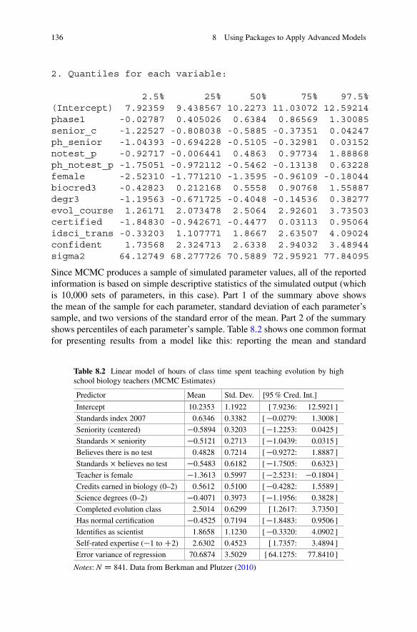
136 8 Using Packages to Apply Advanced Models
2. Quantiles for each variable:
2.5% 25% 50% 75% 97.5%(Intercept) 7.92359 9.438567 10.2273 11.03072 12.59214phase1 -0.02787 0.405026 0.6384 0.86569 1.30085senior_c -1.22527 -0.808038 -0.5885 -0.37351 0.04247ph_senior -1.04393 -0.694228 -0.5105 -0.32981 0.03152notest_p -0.92717 -0.006441 0.4863 0.97734 1.88868ph_notest_p -1.75051 -0.972112 -0.5462 -0.13138 0.63228female -2.52310 -1.771210 -1.3595 -0.96109 -0.18044biocred3 -0.42823 0.212168 0.5558 0.90768 1.55887degr3 -1.19563 -0.671725 -0.4048 -0.14536 0.38277evol_course 1.26171 2.073478 2.5064 2.92601 3.73503certified -1.84830 -0.942671 -0.4477 0.03113 0.95064idsci_trans -0.33203 1.107771 1.8667 2.63507 4.09024confident 1.73568 2.324713 2.6338 2.94032 3.48944sigma2 64.12749 68.277726 70.5889 72.95921 77.84095
Since MCMC produces a sample of simulated parameter values, all of the reportedinformation is based on simple descriptive statistics of the simulated output (whichis 10,000 sets of parameters, in this case). Part 1 of the summary above showsthe mean of the sample for each parameter, standard deviation of each parameter’ssample, and two versions of the standard error of the mean. Part 2 of the summaryshows percentiles of each parameter’s sample. Table 8.2 shows one common formatfor presenting results from a model like this: reporting the mean and standard
Table 8.2 Linear model of hours of class time spent teaching evolution by highschool biology teachers (MCMC Estimates)
Predictor Mean Std. Dev. [95 % Cred. Int.]
Intercept 10.2353 1.1922 [ 7.9236: 12.5921 ]
Standards index 2007 0.6346 0.3382 [ �0.0279: 1.3008 ]
Seniority (centered) �0.5894 0.3203 [ �1.2253: 0.0425 ]
Standards � seniority �0.5121 0.2713 [ �1.0439: 0.0315 ]
Believes there is no test 0.4828 0.7214 [ �0.9272: 1.8887 ]
Standards � believes no test �0.5483 0.6182 [ �1.7505: 0.6323 ]
Teacher is female �1.3613 0.5997 [ �2.5231: �0.1804 ]
Credits earned in biology (0–2) 0.5612 0.5100 [ �0.4282: 1.5589 ]
Science degrees (0–2) �0.4071 0.3973 [ �1.1956: 0.3828 ]
Completed evolution class 2.5014 0.6299 [ 1.2617: 3.7350 ]
Has normal certification �0.4525 0.7194 [ �1.8483: 0.9506 ]
Identifies as scientist 1.8658 1.1230 [ �0.3320: 4.0902 ]
Self-rated expertise (�1 to C2) 2.6302 0.4523 [ 1.7357: 3.4894 ]
Error variance of regression 70.6874 3.5029 [ 64.1275: 77.8410 ]
Notes: N D 841. Data from Berkman and Plutzer (2010)
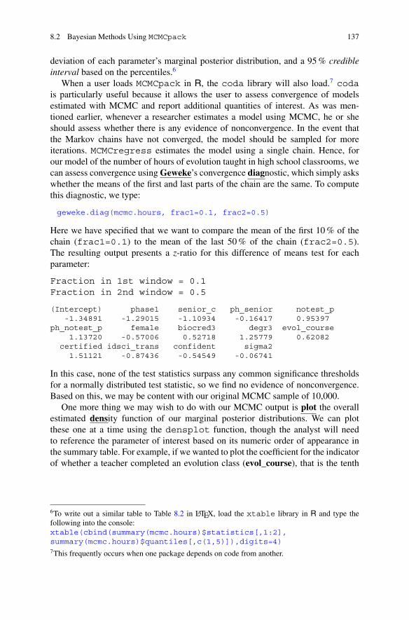
8.2 Bayesian Methods Using MCMCpack 137
deviation of each parameter’s marginal posterior distribution, and a 95 % credibleinterval based on the percentiles.6
When a user loads MCMCpack in R, the coda library will also load.7 codais particularly useful because it allows the user to assess convergence of modelsestimated with MCMC and report additional quantities of interest. As was men-tioned earlier, whenever a researcher estimates a model using MCMC, he or sheshould assess whether there is any evidence of nonconvergence. In the event thatthe Markov chains have not converged, the model should be sampled for moreiterations. MCMCregress estimates the model using a single chain. Hence, forour model of the number of hours of evolution taught in high school classrooms, wecan assess convergence using Geweke’s convergence diagnostic, which simply askswhether the means of the first and last parts of the chain are the same. To computethis diagnostic, we type:
geweke.diag(mcmc.hours, frac1=0.1, frac2=0.5)
Here we have specified that we want to compare the mean of the first 10 % of thechain (frac1=0.1) to the mean of the last 50 % of the chain (frac2=0.5).The resulting output presents a z-ratio for this difference of means test for eachparameter:
Fraction in 1st window = 0.1Fraction in 2nd window = 0.5
(Intercept) phase1 senior_c ph_senior notest_p-1.34891 -1.29015 -1.10934 -0.16417 0.95397
ph_notest_p female biocred3 degr3 evol_course1.13720 -0.57006 0.52718 1.25779 0.62082
certified idsci_trans confident sigma21.51121 -0.87436 -0.54549 -0.06741
In this case, none of the test statistics surpass any common significance thresholdsfor a normally distributed test statistic, so we find no evidence of nonconvergence.Based on this, we may be content with our original MCMC sample of 10,000.
One more thing we may wish to do with our MCMC output is plot the overallestimated density function of our marginal posterior distributions. We can plotthese one at a time using the densplot function, though the analyst will needto reference the parameter of interest based on its numeric order of appearance inthe summary table. For example, if we wanted to plot the coefficient for the indicatorof whether a teacher completed an evolution class (evol_course), that is the tenth
6To write out a similar table to Table 8.2 in LATEX, load the xtable library in R and type thefollowing into the console:xtable(cbind(summary(mcmc.hours)$statistics[,1:2],summary(mcmc.hours)$quantiles[,c(1,5)]),digits=4)7This frequently occurs when one package depends on code from another.

138 8 Using Packages to Apply Advanced Models
0 1 2 3 4 5 1 2 3 4
0.0
0.1
0.2
0.3
0.4
0.5
0.6
0.0
0.2
0.4
0.6
0.8
N = 10000 Bandwidth = 0.1058
a) Completed Evolution Class
N = 10000 Bandwidth = 0.07599
b) Self-Rated Expertise
Fig. 8.1 Density plots of marginal posterior distribution of coefficients for whether the teachercompleted an evolution class and the teacher’s self-rated expertise. Based on an MCMC sample of10,000 iterations (1000 iteration burn-in). (a) Completed evolution class; (b) Self-rated expertise
parameter estimate reported in the table. Similarly, if we wanted to report the densityplot for the coefficient of the teacher’s self-rated expertise (confident), that is thethirteenth parameter reported in the summary table. Hence we could plot each ofthese by typing:
densplot(mcmc.hours[,10])densplot(mcmc.hours[,13])
The resulting density plots are presented in Fig. 8.1. As the figures show, both ofthese marginal posterior distributions have an approximate normal distribution, andthe mode is located near the mean and median reported in our summary output.
8.2.2 Bayesian Logistic Regression
As one additional illustration that MCMCpack estimates a variety of models, weillustrate Bayesian logistic regression, using Singh’s (2014a) data on voting forincumbent parties one last time. If you do not have these data or the library loaded,be sure to do so:
library(MCMCpack)library(foreign)voting<-read.dta("SinghJTP.dta")
To estimate the Bayesian logit model using MCMC, we type:
inc.linear.mcmc<-MCMClogit(votedinc~distanceinc,data=voting)

8.2 Bayesian Methods Using MCMCpack 139
Just as with the MCMCregress command, we have chosen to use the defaults inthis case, but users are encouraged to consider setting their own priors to suit theirneeds. As a matter of fact, this is one case where we will need to raise the number ofiterations in our model. We can check convergence of our model using the Gewekediagnostic:
geweke.diag(inc.linear.mcmc, frac1=0.1, frac2=0.5)
Our output in this case actually shows a significant difference between the means atthe beginning and end of the chain for each parameter:
Fraction in 1st window = 0.1Fraction in 2nd window = 0.5
(Intercept) distanceinc2.680 -1.717
The absolute value of both z-ratios exceeds 1.645, so we can say the mean issignificantly different for each parameter at the 90 % confidence level, which isevidence of nonconvergence.
As a response, we can double both our burn-in period and number of iterationsto 2,000 and 20,000, respectively. The code is:
inc.linear.mcmc.v2<-MCMClogit(votedinc~distanceinc,data=voting,burnin=2000,mcmc=20000)
We can now check for the convergence of this new sample by typing:
geweke.diag(inc.linear.mcmc.v2, frac1=0.1, frac2=0.5)
Our output now shows nonsignificant z-ratios for each parameter, indicating thatthere is no longer evidence of nonconvergence:
Fraction in 1st window = 0.1Fraction in 2nd window = 0.5
(Intercept) distanceinc-1.0975 0.2128
Proceeding with this sample of 20,000, then, if we typesummary(inc.linear.mcmc.v2) into the console, the output is:
Iterations = 2001:22000Thinning interval = 1Number of chains = 1Sample size per chain = 20000
1. Empirical mean and standard deviation for eachvariable, plus standard error of the mean:

140 8 Using Packages to Apply Advanced Models
Mean SD Naive SE Time-series SE(Intercept) 0.1940 0.01846 1.305e-04 0.0003857distanceinc -0.4946 0.00829 5.862e-05 0.0001715
2. Quantiles for each variable:
2.5% 25% 50% 75% 97.5%(Intercept) 0.1573 0.1817 0.1944 0.2063 0.2298distanceinc -0.5105 -0.5003 -0.4946 -0.4890 -0.4783
These results are similar to those that we reported last chapter in Table 7.1,though now we have the opportunity to interpret the findings as a Bayesian. Aswith Bayesian linear regression, if we wished to report density plots of eachparameter, we could apply the densplot command just as before. Overall, thisbrief illustration should show researchers how easy it is to use Bayesian methods inR with MCMCpack. Readers who wish to use more advanced Bayesian methods areencouraged to consult the MCMCpack reference manual and Martin et al. (2011).
8.3 Causal Inference with cem
A prominent innovation in political methodology has been the development ofseveral new matching methods. In brief, matching is a technique designed to selecta subset of field data to make for a fair comparison of individuals who receive atreatment to control individuals who did not receive the treatment. With matching,some observations are thrown away so that the remaining control and treatmentobservations are similar on all covariates that are known to shape the outcome ofinterest. In the absence of experimental data, matching methods serve to allow theresearcher to isolate how the treatment variable affects responses (see Rubin 2006for a thorough treatment of causal inference with matching).
Political Scientists have developed several new matching methods (Imai and vanDyk 2004; Sekhon and Grieve 2012). As an illustration of one of these, and howthe novel technique is implemented in R, we turn to the method developed byIacus et al. (2009, 2011, 2012), Coarsened Exact Matching (CEM). In short, CEMproceeds by temporarily recoding each covariate into an ordered variable that lumpssimilar values of the covariate together. The data are then sorted into strata basedon their profiles of the coarsened variables, and any observations in a stratum thatdoes not contain at least one treatment and one control unit are thrown away. Theresulting sample should show much more balance in the control variables betweenthe treated and control observations. In R, this technique is implemented with thecem command within the cem package.

8.3 Causal Inference with cem 141
8.3.1 Covariate Imbalance, Implementing CEM, and the ATT
As our example data, we return to LaLonde’s (1986) study of the NationalSupported Work Demonstration that we previously examined in Chaps. 4 and 5. Ourtreatment variable (treated) indicates if the individual received the treatment fromthe National Supported Work Demonstration, meaning the person was placed in aprivate sector job for a year with public funds covering the labor costs. We wouldlike to know the causal effect of this treatment on the individual’s earnings in1978, after the treatment was completed (re78). In Sect. 5.1.1 we did a naïve testof this hypothesis by simply using a difference of means test between the treatedindividuals and the control group without controlling for any of the other variablesthat are likely to affect annual income. In our naïve test, we found that income washigher for the treated group, but now we can ask what the estimated effect is whenwe account for other important covariates.
As was noted in earlier chapters, LaLonde’s data are already included in the cempackage, so we can load these data easily if we have already loaded the cem library.The following lines of code clean up, install cem (in case you have not already),opens cem, and loads LaLonde’s data (named LL):8
rm(list=ls())install.packages("cem")library(cem)data(LL)
An important task when using matching methods is assessing the degree to whichthe data are balanced, or the degree to which treated cases have a similar distributionof covariate values relative to the control group. We can assess the degree to whichour treatment and control groups have differing distributions with the imbalancecommand. In the code below, we first increase the penalty for scientific notation(an option if you prefer decimal notation). Then, we create a vector naming thevariables we do not want to assess balance for—the treatment variable (treated)and the outcome of interest (re78). All other variables in the dataset are covariatesthat we believe can shape income in 1978, so we would like to have balance onthem. In the last line, we actually call the imbalance command.
options(scipen=8)todrop <- c("treated","re78")imbalance(group=LL$treated, data=LL, drop=todrop)
Within the imbalance command, the group argument is our treatment variablethat defines the two groups for which we want to compare the covariate distributions.The data argument names the dataset we are using, and the drop option allows usomit certain variables from the dataset when assessing covariate balance. Our outputfrom this command is as follows:
8LaLonde’s data is also available in the file LL.csv, available in the Dataverse (see page vii) orthe chapter content (see page 125).
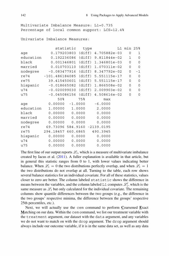
142 8 Using Packages to Apply Advanced Models
Multivariate Imbalance Measure: L1=0.735Percentage of local common support: LCS=12.4%
Univariate Imbalance Measures:
statistic type L1 min 25%age 0.179203803 (diff) 4.705882e-03 0 1education 0.192236086 (diff) 9.811844e-02 1 0black 0.001346801 (diff) 1.346801e-03 0 0married 0.010703110 (diff) 1.070311e-02 0 0nodegree -0.083477916 (diff) 8.347792e-02 0 -1re74 -101.486184085 (diff) 5.551115e-17 0 0re75 39.415450601 (diff) 5.551115e-17 0 0hispanic -0.018665082 (diff) 1.866508e-02 0 0u74 -0.020099030 (diff) 2.009903e-02 0 0u75 -0.045086156 (diff) 4.508616e-02 0 0
50% 75% maxage 0.00000 -1.0000 -6.0000education 1.00000 1.0000 2.0000black 0.00000 0.0000 0.0000married 0.00000 0.0000 0.0000nodegree 0.00000 0.0000 0.0000re74 69.73096 584.9160 -2139.0195re75 294.18457 660.6865 490.3945hispanic 0.00000 0.0000 0.0000u74 0.00000 0.0000 0.0000u75 0.00000 0.0000 0.0000
The first line of our output reports L1, which is a measure of multivariate imbalancecreated by Iacus et al. (2011). A fuller explanation is available in that article, butin general this statistic ranges from 0 to 1, with lower values indicating betterbalance. When L1 D 0 the two distributions perfectly overlap, and when L1 D 1
the two distributions do not overlap at all. Turning to the table, each row showsseveral balance statistics for an individual covariate. For all of these statistics, valuescloser to zero are better. The column labeled statistic shows the difference inmeans between the variables, and the column labeled L1 computes L j
1 , which is thesame measure as L1 but only calculated for the individual covariate. The remainingcolumns show quantile differences between the two groups (e.g., the difference inthe two groups’ respective minima, the difference between the groups’ respective25th percentiles, etc.).
Next, we will actually use the cem command to perform Coarsened ExactMatching on our data. Within the cem command, we list our treatment variable withthe treatment argument, our dataset with the data argument, and any variableswe do not want to match on with the drop argument. The drop argument shouldalways include our outcome variable, if it is in the same data set, as well as any data

8.3 Causal Inference with cem 143
indices or irrelevant variables. We could use a vector to list all of the variables wewant to be ignored, as we did with the imbalance command before, but in thiscase, only the outcome re78 needs to be skipped. We type:
cem.match.1 <- cem(treatment="treated", data=LL, drop="re78")cem.match.1
Our immediate output from this is simply the following:
G0 G1All 425 297Matched 222 163Unmatched 203 134
This tells us that our original data had 425 control observations and 297 treatedobservations. CEM included 222 of the control and 163 of the treated observationsin the matched sample, and the rest are pruned away. To be clear: All observationsare still contained in the original LL dataset, but now the object cem.match.1itemizes which observations are matched or not.
Since CEM proceeds by grouping similar values of covariates into strata, animportant feature of this is how we set the ordered intervals of each predictor incoarsening. The cem command has reasonable defaults if the user does not set theseintervals, but it is important to record what the intervals are. To see what our intervalswere for the values of our predictors, we could type: cem.match.1$breaks.This would give us the following output:
$age[1] 17.0 20.8 24.6 28.4 32.2 36.0 39.8 43.6 47.4 51.2 55.0
$education[1] 3.0 4.3 5.6 6.9 8.2 9.5 10.8 12.1 13.4 14.7 16.0
$black[1] 0.0 0.1 0.2 0.3 0.4 0.5 0.6 0.7 0.8 0.9 1.0
$married[1] 0.0 0.1 0.2 0.3 0.4 0.5 0.6 0.7 0.8 0.9 1.0
$nodegree[1] 0.0 0.1 0.2 0.3 0.4 0.5 0.6 0.7 0.8 0.9 1.0
$re74[1] 0.000 3957.068 7914.136 11871.204 15828.272 19785.340[7] 23742.408 27699.476 31656.544 35613.612 39570.680
$re75[1] 0.000 3743.166 7486.332 11229.498 14972.664 18715.830[7] 22458.996 26202.162 29945.328 33688.494 37431.660
$hispanic[1] 0.0 0.1 0.2 0.3 0.4 0.5 0.6 0.7 0.8 0.9 1.0

144 8 Using Packages to Apply Advanced Models
$u74[1] 0.0 0.1 0.2 0.3 0.4 0.5 0.6 0.7 0.8 0.9 1.0
$u75[1] 0.0 0.1 0.2 0.3 0.4 0.5 0.6 0.7 0.8 0.9 1.0
To illustrate what this means, consider age. The lowest category of coarsenedage lumps together everyone aged 17–20.8, the second category lumps everyoneaged 20.8–24.6, and so forth. Variables like black, married, nodegree,hispanic, u74, and u75 are actually binary, so most of the categories beingcreated are unnecessary, though empty bins will not hurt our analysis. Of course,users are not required to use software defaults, and Iacus et al. urge researchers touse substantive knowledge of each variable’s measurement to set the ranges of thecoarsening bins (2012, p. 9). Section 8.3.2 offers details on doing this.
Now we can assess imbalance in the new matched sample by typing:
imbalance(LL$treated[cem.match.1$matched],LL[cem.match.1$matched,], drop=todrop)
Our output from this is as follows:
Multivariate Imbalance Measure: L1=0.592Percentage of local common support: LCS=25.2%
Univariate Imbalance Measures:
statistic type L1 min 25% 50%age -0.42486044 (diff) 0.00000000 0 -1 -2.0000education -0.10855027 (diff) 0.10902006 0 0 -1.0000black -0.01771403 (diff) 0.01771403 0 0 0.0000married -0.01630465 (diff) 0.01630465 0 0 0.0000nodegree 0.09022827 (diff) 0.09022827 0 0 0.0000re74 -119.33548135 (diff) 0.00000000 0 0 0.0000re75 -50.01527694 (diff) 0.00000000 0 0 -49.3559hispanic 0.01561377 (diff) 0.01561377 0 0 0.0000u74 0.01619411 (diff) 0.01619411 0 0 0.0000u75 0.02310286 (diff) 0.02310286 0 0 0.0000
75% maxage 0.00 1.000education 0.00 0.000black 0.00 0.000married 0.00 0.000nodegree 0.00 0.000re74 -492.95 416.416re75 -136.45 -852.252hispanic 0.00 0.000u74 0.00 0.000u75 0.00 0.000
Compare this to the original data. We now have L1 D 0:592, which is less thanour score of 0.735 for the raw data, indicating that multivariate balance is better inthe matched sample. Turning to the individual covariates, you can see somethingof a mixed bag, but overall the balance looks better. For instance, with age the

8.3 Causal Inference with cem 145
difference in means is actually a bit larger in absolute value with the matched sample(0.42) than the raw data (0.18). However, L age
1 is now minuscule in the matchedsample, and less than the 0.0047 value for the raw data. This is likely on account ofthe fact that the raw data has a larger discrepancy at the high end than the matchedsample has. The user now must decide whether the treated and control cases aresufficiently balanced or whether to try other coarsenings to improve balance.
If the user is satisfied with the level of balance, he or she can proceed to estimatethe Average Treatment effect on the Treated (ATT) using the command att. Thisquantity represents the causal effect on the kind of individual who received thetreatment. In this command we specify what our matched sample is using the objargument, the outcome variable (re78) and treatment (treated) using the formulaargument, and our data using the data argument. This gives us:
est.att.1 <- att(obj=cem.match.1, formula=re78~treated, data=LL)est.att.1
Our output from this is:
G0 G1All 425 297Matched 222 163Unmatched 203 134
Linear regression model on CEM matched data:
SATT point estimate: 550.962564 (p.value=0.368242)95% conf. interval: [-647.777701, 1749.702830]
The output recaps the features of our matched sample and then reports our estimateof the sample average treatment effect on the treated (SATT): We estimate in oursample that individuals receiving the treatment earned $551 more on average thanthose who did not receive the treatment. However, this effect is not statisticallydiscernible from zero (p D 0:368). This is a markedly different conclusion from theone we drew in Chap. 5, when we observed a $886 difference that was statisticallysignificant. This illustrates the importance of statistical control.
8.3.2 Exploring Different CEM Solutions
As a final point, if a researcher is not happy with the level of balance or the samplesize in the matched sample, then a tool for finding better balance is the cemspacecommand. This command randomly produces several different coarsenings forthe control variables (250 different coarsenings by default). The command thenplots the level of balance against the number of treated observations included inthe matched sample. The following code calls this command:

146 8 Using Packages to Apply Advanced Models
cem.explore<-cemspace(treatment="treated",data=LL,drop="re78")
The syntax of cemspace is similar to cem, though two more options are important:minimal and maximal. These establish what the minimum and maximumallowed number of coarsened intervals is for the variables. The command aboveuses the defaults of 1 and 5, which means that no more than five intervals maybe included for a variable. Hence, all matched samples from this command willbe coarser than what we used in Sect. 8.3.1, and therefore less balanced. The usercould, however, increase maximal to 12 or even a higher number to create finerintervals and potentially improve the balance over our prior result.
Our output from cemspace is shown in Fig. 8.2. On account of the randomelement in choosing coarsenings, your results will not exactly match this figure.Figure 8.2a shows the interactive figure that opens up. The horizontal axis of thisfigure shows the number of matched treatment units in descending order, whilethe vertical axis shows the level of imbalance. In general, a matched sample atthe bottom-left corner of the graph would be ideal as that would indicate the bestbalance (reducing bias) and the largest sample (increasing efficiency). Normally,though, we have to make a choice on this tradeoff, generally putting a bit moreweight on minimizing imbalance. By clicking on different points on the graph, thesecond window that cemspace creates, shown in Fig. 8.2b will show the intervalsused in that particular coarsening. The user can copy the vectors of the intervalcutpoints and paste them into his or her own code. Note: R will not proceed withnew commands until these two windows are closed.
In Fig. 8.2a, one of the potential coarsenings has been chosen, and it is high-lighted and yellow. If we want to implement this coarsening, we can copy the vectorsshown in the second window illustrated in Fig. 8.2b. Pasting these into our own Rscript produces the following code:
Total units=297, ML1=0.414
number matched, scaled as 1/sqrt(matched)
med
ian
of L
1 pr
ofile
raw
a) Plot Window b) X11 Window
0.25
0.30
0.35
0.40
297 287 278 269 260 252 244
Fig. 8.2 Plot of balance statistics for 250 matched samples from random coarsenings againstnumber of treated observations included in the respective matched sample. (a) Plot window;(b) X11 window

8.4 Legislative Roll Call Analysis with wnominate 147
age.cut<-c(17, 26.5, 36, 45.5, 55)education.cut<-c(3, 6.25, 9.5, 12.75, 16)black.cut<-c(0, 0.5, 1)married.cut<-c(0, 0.5, 1)nodegree.cut<-c(0, 0.5, 1)re74.cut<-c(0, 19785.34, 39570.68)re75.cut<-c(0, 9357.92, 18715.83, 28073.75, 37431.66)hispanic.cut<-c(0, 0.5, 1)u74.cut<-c(0, 0.5, 1)u75.cut<-c(0, 1)new.cuts<-list(age=age.cut, education=education.cut,
black=black.cut, married=married.cut,nodegree=nodegree.cut, re74=re74.cut, re75=re75.cut,hispanic=hispanic.cut, u74=u74.cut, u75=u75.cut)
We end this code by creating a list of all of these vectors. While our vectors herehave been created using a coarsening created by cemspace, this is the procedurea programmer would use to create his or her own cutpoints for the intervals.By substituting the vectors above with user-created cutpoint vectors, a researchercan use his or her own knowledge of the variables’ measurement to coarsen.
Once we have defined our own cutpoints, either by using cemspace orsubstantive knowledge, we can now apply CEM with the following code:
cem.match.2 <- cem(treatment="treated", data=LL, drop="re78",cutpoints=new.cuts)
Our key addition here is the use of the cutpoints option, where we input our listof intervals. Just as in Sect. 8.3.1, we can now assess the qualities of the matchedsample, imbalance levels, and compute the ATT if we wish:
cem.match.2imbalance(LL$treated[cem.match.2$matched],
LL[cem.match.2$matched,], drop=todrop)est.att.2 <- att(obj=cem.match.2, formula=re78~treated, data=LL)est.att.2
In this case, in part because of the coarser bins we are using, the balance is worsethat what we found in the previous section. Hence, we would be better off in thiscase sticking with our first result. The reader is encouraged to try to find a coarseningthat produces better balance than the software defaults.
8.4 Legislative Roll Call Analysis with wnominate
Methodologists in Political Science and other disciplines have developed a widearray of measurement models, several of which are available for user implemen-tation in R. Without a doubt, one of the most prominent measurement models inthe discipline is NOMINATE, short for nominal three-step estimation (McCartyet al. 1997; Poole and Rosenthal 1997; Poole et al. 2011). The NOMINATEmodel analyzes roll call data from legislative votes, placing legislators, and policyalternatives they vote on in ideological space. The model is particularly prominentbecause Poole, Rosenthal, and colleagues make DW-NOMINATE scores available

148 8 Using Packages to Apply Advanced Models
for both the US House of Representatives and Senate for every term of Congress.Countless authors have used these data, typically interpreting the first dimensionscore as a scale of liberal-conservative ideology.
In brief, the basic logic of the model draws from the spatial proximity modelof politics, which essentially states that both individuals’ ideological preferencesand available policy alternatives can be represented in geometric space of one ormore dimensions. An individual generally will vote for the policy choice that isclosest in space to his or her own ideological ideal point (Black 1958; Downs1957; Hotelling 1929). The NOMINATE model is based on these assumptions, andplaces legislators and policy options in ideological space based on how legislators’votes divide over the course of many roll call votes and when legislators behaveunpredictably (producing errors in the model). For example, in the US Congress,liberal members typically vote differently from conservative members, and theextreme ideologues are the most likely to be in a small minority whenever thereis wide consensus on an issue. Before applying the NOMINATE method to yourown data—and even before downloading pre-measured DW-NOMINATE data toinclude in a model you estimate—be sure to read more about the method and itsassumptions because thoroughly understanding how a method works is essentialbefore using it. In particular, Chap. 2 and Appendix A from Poole and Rosenthal(1997) and Appendix A from McCarty et al. (1997) offer detailed, yet intuitive,descriptions of how the method works.
In R, the wnominate package implements W-NOMINATE, which is a versionof the NOMINATE algorithm that is intended only to be applied to a singlelegislature. W-NOMINATE scores are internally valid, so it is fair to comparelegislators’ scores within a single dataset. However, the scores cannot be externallycompared to scores when W-NOMINATE is applied to a different term of thelegislature or a different body of actors altogether. Hence, it is a good method fortrying to make cross-sectional comparisons among legislators of the same body.
While the most common application for W-NOMINATE has been theUS Congress, the method could be applied to any legislative body. To that end,the working example in this section focuses on roll call votes cast in the UnitedNations. This UN dataset is available in the wnominate package, and it pools 237roll call votes cast in the first three sessions of the UN (1946–1949) by 59 membernations. The variables are labeled V1 to V239. V1 is the name of the membernation, and V2 is a categorical variable either coded as “WP” for a member of theWarsaw Pact, or “Other” for all other nations. The remaining variables sequentiallyidentify roll call votes.
To begin, we clean up, install the wnominate package the first time we use it,load the library, and load the UN data:9
rm(list=ls())install.packages("wnominate")library(wnominate)data(UN)
9The UN data is also available in the file UN.csv, available in the Dataverse (see page vii) or thechapter content (see page 125)

8.4 Legislative Roll Call Analysis with wnominate 149
Once the data are loaded, they can be viewed with the standard commands suchas fix, but for a quick view of what the data look like, we could simply type:head(UN[,1:15]). This will show the structure of the data through the first 13roll call votes.
Before we can apply W-NOMINATE, we have to reformat the data to an objectof class rollcall. To do this, we first need to redefine our UN dataset as a matrix,and split the names of the countries, whether the country was in the Warsaw Pact,and the set of roll calls into three separate parts:
UN<-as.matrix(UN)UN.2<-UN[,-c(1,2)]UNnames<-UN[,1]legData<-matrix(UN[,2],length(UN[,2]),1)
The first line turned the UN data frame into a matrix. (For more on matrix commandsin R, see Chap. 10.) The second line created a new matrix, which we have namedUN.2, which has eliminated the first two columns (country name and member ofWarsaw Pact) to leave only the roll calls. The third line exported the names of thenations into the vector UNnames. (In many other settings, this would instead be thename of the legislator or an identification variable.) Lastly, our variable of whethera nation was in the Warsaw Pact has been saved as a one-column matrix namedlegData. (In many other settings, this would be a legislator’s political party.) Oncewe have these components together, we can use the rollcall command to definea rollcall-class object that we name rc as follows:
rc<-rollcall(data=UN.2,yea=c(1,2,3),nay=c(4,5,6),missing=c(7,8,9),notInLegis=0,legis.names=UNnames,legis.data=legData,desc="UN Votes",source="voteview.com")
We specify our matrix of roll call votes with the data argument. Based on howthe data in the roll call matrix are coded, we use the yea, nay, and missingarguments to translate numeric codes into their substantive meaning. Additionally,notInLegis allows us to specify a code that specifically means that the legislatorwas not a member at the time of the vote (e.g., a legislator died or resigned). Wehave no such case in these data, but the default value is notInLegis=9, and9 means something else to us, so we need to specify an unused code of 0. Withlegis.names we specify the names of the voters, and with legis.data wespecify additional variables about our voters. Lastly, desc and source allow usto record additional information about our data.
With our data formatted properly, we can now apply the W-NOMINATE model.the command is simply called wnominate:
result<-wnominate(rcObject=rc,polarity=c(1,1))
With the rcObject argument, we simply name our properly formatted data. Thepolarity argument, by contrast, requires substantive input from the researcher:The user should specify a vector that lists which observation should clearly fallon the positive side of each dimension estimated. Given the politics of the Cold

150 8 Using Packages to Apply Advanced Models
War, we use observation #1, the USA, as the anchor on both dimensions weestimate. By default, wnominate places voters in two-dimensional ideologicalspace (though this could be changed by specifying the dims option).
To view the results of our estimation, we can start by typing:summary(result). This prints the following output.
SUMMARY OF W-NOMINATE OBJECT----------------------------
Number of Legislators: 59 (0 legislators deleted)Number of Votes: 219 (18 votes deleted)Number of Dimensions: 2Predicted Yeas: 4693 of 5039 (93.1%) predictionscorrectPredicted Nays: 4125 of 4488 (91.9%) predictionscorrectCorrect Classification: 89.5% 92.56%APRE: 0.574 0.698GMP: 0.783 0.841
The first 10 legislator estimates are:coord1D coord2D
United States 0.939 0.344Canada 0.932 0.362Cuba 0.520 -0.385Haiti 0.362 -0.131Dominican Rep 0.796 -0.223Mexico 0.459 0.027Guatemala 0.382 0.364Honduras 0.588 -0.266El Salvador 0.888 -0.460Nicaragua 0.876 -0.301
The output begins by recapping several descriptive features of our data and thenturns to fit indices. It lists, for instance the correct prediction of yeas and nays,and then under “Correct Classification” lists the percent correctly predicted bythe first dimension alone and then both dimensions together. At 89.5 %, the firstdimension can explain a lot by itself. The output ends by listing the estimates forour first 10 observations. As can be seen, the USA does take a positive value on bothdimensions, per our specification in the model.
We can obtain additional output by typing: plot(result). The result of thiscommand is presented in Fig. 8.3. The top-left panel visualizes the W-NOMINATEscores for the 59 voting nations. The horizontal axis is the first dimension of thescore, the vertical axis is the second dimension, and each point represents a nation’sposition. Hence, in the two-dimensional ideological space defined internally to UN

8.4 Legislative Roll Call Analysis with wnominate 151
−1.
0−
0.5
0.0
0.5
1.0
−1.0 −0.5 0.0 0.5 1.0
W−NOMINATE Coordinates
First Dimension
Sec
ond
Dim
ensi
on
Leg
Cutting Line Angles
Angle in Degrees
Cou
nt
0 20 40 60 80 100 130 160
010
2030
40
1 3 5 7 9 11 13 15 17 19
12
3
Scree Plot
Dimension
Eig
enva
lue
−1.0 −0.5 0.0 0.5 1.0
−1.
0−
0.5
0.0
0.5
1.0
Cutting Lines
First Dimension
Sec
ond
Dim
ensi
on
Fig. 8.3 Output plot from estimating W-NOMINATE scores from the first three sessions of theUnited Nations
proceedings, this is where each nation falls. The bottom-left panel shows a screeplot, which lists the eigenvalue associated with each dimension. Larger eigenvaluesindicate that a dimension has more explanatory power. As in all scree plots, eachadditional dimension has lower explanatory value than the previous one.10 The top-right panel shows the distribution of the angles of the cutting lines. The cutting linesdivide yea from nay votes on a given issue. The fact that so many cutting lines arenear the 90ı mark indicates that the first dimension is important for many of the
10When choosing how many dimensions to include in a measurement model, many scholars usethe “elbow rule,” meaning they do not include any dimensions past a visual elbow in the scree plot.In this case, a scholar certainly would not include more than three dimensions, and may be contentwith two. Another common cutoff is to include any dimension for which the eigenvalue exceeds 1,which would have us stop at two dimensions.

152 8 Using Packages to Apply Advanced Models
votes. Finally, the bottom-right panel shows the Coombs Mesh from this model—avisualization of how all of the cutting lines on the 237 votes come together in asingle space.
If the user is satisfied with the results of this measurement model, then it isstraightforward to write the scores into a useable data format. Withinour wnominate output named result we can call the attribute namedlegislators, which saves our ideal points for all countries, any non-roll callvariables we specified (e.g., Warsaw Pact or not), and a variety of other measures.We save this as a new data frame named scores and then write that to a CSV file:
scores<-result$legislatorswrite.csv(scores,"UNscores.csv")
Just remember to use the setwd command to specify the folder in which you wishto save the output file.
Once we have our W-NOMINATE ideal points in a separate data frame, we cando anything we normally would with data in R, such as draw our own graphs.Suppose we wanted to reproduce our own graph of the ideal points, but we wantedto mark which nations were members of the Warsaw Pact versus those that were not.We could easily do this using our scores data. The easiest way to do this mightbe to use the subset command to create separate data frames of our two groups:
wp.scores<-subset(scores, V1=="WP")other.scores<-subset(scores, V1=="Other")
Once we have these subsets in hand, we can create the relevant graph in three linesof code.
plot(x=other.scores$coord1D, y=other.scores$coord2D,xlab="First Dimension", ylab="Second Dimension",xlim=c(-1,1), ylim=c(-1,1), asp=1)
points(x=wp.scores$coord1D, y=wp.scores$coord2D,pch=3,col=’red’)
legend(x=-1,y=-.75,legend=c("Other","Warsaw Pact"),col=c("black","red"),pch=c(1,3))
In the call to plot, we graph the 53 nations that were not members of the WarsawPact, putting the first dimension on the horizontal axis, and the second on the verticalaxis. We label our axes appropriately using xlab and ylab. We also set the boundsof our graph as running from �1 to 1 on both dimensions, as scores are constrainedto fall in these ranges. Importantly, we guarantee that the scale of the two dimensionsis the same, as we generally should for this kind of measurement model, by settingthe aspect ratio to 1 (asp=1). On the second line of code, we use the pointscommand to add the six observations that were in the Warsaw Pact, coloring theseobservations red and using a different plotting character. Lastly, we add a legend.
Figure 8.4 presents the output from our code. This graph immediately conveysthat the first dimension is capturing the Cold War cleavage between the USA andits allies versus the Soviet Union and its allies. We specified that the USA wouldtake positive coordinates on both dimensions, so we can see that the Soviet allies

8.5 Practice Problems 153
−1.
0−
0.5
0.0
0.5
1.0
−1.0 −0.5 0.0 0.5 1.0First Dimension
Sec
ond
Dim
ensi
on
OtherWarsaw Pact
Fig. 8.4 Plot of first and second dimensions of W-NOMINATE scores from the first three sessionsof the United Nations. A red cross indicates a member of the Warsaw Pact, and a black circleindicates all other UN members (Color figure online)
(represented with red crosses) are at the extremes of negative values on the firstdimension.
To recap, this chapter has illustrated four examples of how to use R packagesto implement advanced methods. The fact that these packages are freely availablemakes cutting-edge work in political methodology and from a variety of disciplinesreadily available to any R user. No book could possibly showcase all of theresearcher-contributed packages that are available, not least because new packagesare being made available on a regular basis. The next time you find yourself facinga taxing methodological problem, you may want to check the CRAN servers to seeif someone has already written a program that provides what you need.
8.5 Practice Problems
This set of practice problems considers each of the example libraries in turn, andthen suggests you try using a brand new package that has not been discussed in thischapter. Each question calls for a unique data set.
1. Multilevel Logistic Regression: Revisit Singh’s (2015) data on voter turnout asa function of compulsory voting rules and several other predictors. If you do nothave the file stdSingh.dta, please download it from the Dataverse (see pagevii) or the chapter content (see page 125). (These data were first introduced in

154 8 Using Packages to Apply Advanced Models
Sect. 7.4.) Refit this logistic regression model using the glmer command, andinclude a random intercept by country-year (cntryyear). Recall that the outcomeis turnout (voted). The severity of compulsory voting rules (severity) is inter-acted with the first five predictors: age (age), political knowledge (polinfrel),income (income), efficacy (efficacy), and partisanship (partyID). Five morepredictors should be included only for additive effects: district magnitude(dist_magnitude), number of parties (enep), victory margin (vicmarg_dist),parliamentary system (parliamentary), and per capita GDP (development).Again, all of the predictor variables have been standardized. What do you learnfrom this multilevel logistic regression model estimated with glmer that you donot learn from a pooled logistic regression model estimated with glm?
2. Bayesian Poisson model with MCMC: Determine how to estimate a Poissonmodel with MCMC using MCMCpack. Reload Peake and Eshbaugh-Soha’s(2008) data on energy policy news coverage, last discussed in Sect. 7.3. If youdo not have the file PESenergy.csv, you may download it from the Dataverse(see page vii) or the chapter content (see page 125). Estimate a Bayesian Poissonmodel in which the outcome is energy coverage (Energy), and the inputs aresix indicators for presidential speeches (rmn1173, grf0175, grf575, jec477,jec1177, and jec479), an indicator for the Arab oil embargo (embargo), anindicator for the Iran hostage crisis (hostages), the price of oil (oilc), presidentialapproval (Approval), and the unemployment rate (Unemploy). Use a Geweketest to determine whether there is any evidence of nonconvergence. How shouldyou change your code in R if nonconvergence is an issue? Summarize yourresults in a table, and show a density plot of the partial coefficient on RichardNixon’s November 1973 speech (rmn1173).
3. Coarsened Exact Matching: In Chap. 5, the practice problems introduced Alvarezet al.’s (2013) data from a field experiment in Salta, Argentina in which somevoters cast ballots through e-voting, and others voted in the traditional setting.Load the foreign library and open the data in Stata format. If you do not havethe file alpl2013.dta, you may download it from the Dataverse (see page vii)or the chapter content (see page 125). In this example, the treatment variable iswhether the voter used e-voting or traditional voting (EV). The covariates are agegroup (age_group), education (educ), white collar worker (white_collar), not afull-time worker (not_full_time), male (male), a count variable for number ofsix possible technological devices used (tech), and an ordinal scale for politicalknowledge (pol_info). Use the cem library to answer the following:
a. How balanced are the treatment and control observations in the raw data?b. Conduct coarsened exact matching with the cem command. How much has
the balance improved as a result?c. Consider three possible response variables: whether the voter evaluated the
voting experience positively (eval_voting), whether the voter evaluated thespeed of voting as quick (speed), and whether the voter is sure his or her voteis being counted (sure_counted). What is the average treatment effect on thetreated (ATT) on your matched dataset for each of these three responses?

8.5 Practice Problems 155
d. How do your estimates of the average treatment effects on the treated differfrom simple difference-of-means tests?
4. W-NOMINATE: Back in Sect. 2.1, we introduced Lewis and Poole’s roll call datafor the 113th US Senate. Consult the code there to read these data, which are infixed width format. The file name is sen113kh.ord, and it is available fromthe Dataverse (see page vii) and the chapter content (see page 125).
a. Format the data as a matrix and create the following: a separate matrix just ofthe 657 roll calls, a vector of the ICPSR identification numbers, and a matrixof the non-roll call variables. Use all of these to create a rollcall-classobject. The roll call votes are coded as follows: 1 D Yea; 6 D Nay; 7 &9 D missing, and 0 D not a member.
b. Estimate a two-dimensional W-NOMINATE model for this roll call object.From the summary of your results, report the following: How many legislatorswere deleted? How many votes were deleted? Was was the overall correctclassification?
c. Examine the output plot of your estimated model, including theW-NOMINATE coordinates and the scree plot. Based on the scree plot,how many dimensions do you believe are sufficient to characterize votingbehavior in the 113th Senate? Why?
5. Bonus: Try learning how to use a package you have never used before. Install theAmelia package, which conducts multiple imputation for missing data. Have alook at Honaker et al.’s (2011) article in the Journal of Statistical Software to geta feel for the logic of multiple imputation and to learn how to do this in R. Fit alinear model on imputed datasets using the freetrade data from the Amelialibrary. What do you find?
Chapter 9Time Series Analysis
Most of the methods described so far in this book are oriented primarily atcross-sectional analysis, or the study of a sample of data taken at the same point intime. In this chapter, we turn to methods for modeling a time series, or a variable thatis observed sequentially at regular intervals over time (e.g., daily, weekly, monthly,quarterly, or annually). Time series data frequently have trends and complex errorprocesses, so failing to account for these features can produce spurious results(Granger and Newbold 1974). Several approaches for time series analysis haveemerged to address these problems and prevent false inferences. Within PoliticalScience, scholars of public opinion, political economy, international conflict, andseveral other subjects regularly work with time-referenced data, so adequate toolsfor time series analysis are important in political analysis.
Many researchers do not think of R as a program for time series analysis, insteadusing specialty software such as Autobox, EViews, or RATS. Even SAS and Statatend to get more attention for time series analysis than R does. However, R actuallyhas a wide array of commands for time series models, particularly through the TSAand vars packages. In this chapter, we will illustrate three approaches to time seriesanalysis in R: the Box–Jenkins approach, extensions to linear models estimated withleast squares, and vector autoregression. This is not an exhaustive list of the toolsavailable for studying time series, but is just meant to introduce a few prominentmethods. See Sect. 9.4 for some further reading on time series.
Both the Box–Jenkins approach and extensions to linear models are examplesof single equation time series models. Both approaches treat one time series asan outcome variable and fit a model of that outcome that can be stated in oneequation, much like the regression models of previous chapters can be stated ina single equation. Since both approaches fall into this broad category, the working
Electronic supplementary material: The online version of this chapter(doi: 10.1007/978-3-319-23446-5_9) contains supplementary material, which is available toauthorized users.
© Springer International Publishing Switzerland 2015J.E. Monogan III, Political Analysis Using R, Use R!,DOI 10.1007/978-3-319-23446-5_9
157
158 9 Time Series Analysis
dataset we use for both the Box–Jenkins approach and extensions to linear modelswill be Peake and Eshbaugh-Soha’s (2008) monthly data on television coverage ofenergy policy that was first introduced in Chap. 3. By contrast, vector autoregressionis a multiple equation time series model (for further details on this distinction, seeBrandt and Williams 2007 or Lütkepohl 2005). With a vector autoregression model,two or more time series are considered endogenous, so multiple equations arerequired to fully specify the model. This is important because endogenous variablesmay affect each other, and to interpret an input variable’s effect, the broader contextof the full system must be considered. Since multiple equation models have such adifferent specification, when discussing vector autoregression the working examplewill be Brandt and Freeman’s (2006) analysis of weekly political actions in theIsraeli–Palestinian conflict; more details will be raised once we get to that section.
9.1 The Box–Jenkins Method
The Box–Jenkins approach to time series relies on autoregressive integrated movingaverage (ARIMA) models to capture the error process in the data. For a comprehen-sive explanation of this approach, see Box et al. (2008). The basic logic of thisapproach is that a time series should be filtered, or prewhitened, of any trendsand error processes before attempting to fit an inferential model. Once a modelof the noise, or error, has been specified, then the researcher can proceed to testhypotheses.1 On account of nonlinear functional forms that often emerge in ARIMAand transfer function models, these usually are estimated with maximum likelihood.
To illustrate the process from identifying an error model to testing a hypothesis,we revisit Peake and Eshbaugh-Soha’s (2008) monthly time series on energy policycoverage. We start by reloading our data:2
pres.energy<-read.csv("PESenergy.csv")
Our outcome variable is the number of energy-related stories on nightly televisionnews by month (Energy). A good first step is to plot the series being studied to seeif any trends or other features are immediately apparent. Look back at Fig. 3.6 forthe example code we used to plot our outcome variable (Energy) and the price ofoil, which is one of the predictors (oilc). As a first look at the news coverage series,the data appear to be stationary, meaning that they hover around a mean withouttrending in one direction or showing an integrated pattern.
As a substantively important point about time series in general, the distinctionbetween stationary and nonstationary series is important. Many time series methods
1Many use ARIMA models for forecasting future values of a series. ARIMA models themselves areatheoretical, but often can be effective for prediction. Since most Political Science work involvestesting theoretically motivated hypotheses, this section focuses more on the role ARIMA modelscan serve to set up inferential models.2If you do not have the data file PESenergy.csv already, you can download it from theDataverse (see page vii) or the online chapter content (see page 155).

9.1 The Box–Jenkins Method 159
are designed specifically for modeling stationary series, so applying them to anonstationary series can be problematic. A stationary series is one for which themean and variance do not change conditional on time, and the series does nottrend in one direction. If a stationary series is disturbed, or moved to a higher orlower value, it eventually returns back to an equilibrium level. The two kinds ofnonstationary series are trending series and integrated series. With a trending series,as its name implies, the conditional average changes over time, typically rising orfalling consistently. For example, nominal prices of consumer goods may rise orfall from one quarter to the next, but the average value tends to rise over time. Anintegrated series, also called a unit root series, does not have an equilibrium valueand has the feature of “long memory.” This means that if something changes thevalue of a series, then future values of the series will be affected by that change longinto the future. For instance, suppose the Dow Jones Industrial Average dropped300 points in 1 day, from 18,200 to 17,900. In such a case, future values of theDow will be based on the new value of 17,900 plus however much the value rose orfell each subsequent day, and the Dow will not tend to revert back to earlier values.Importantly, by differencing the current value of a series from its previous value,or measuring how much a series changed from one time to the next, trending orintegrated series can be made stationary. Hence, many models for stationary seriescan be applied to the difference of a nonstationary series. Whenever doing appliedtime series work always look at the graph of the series, such as Fig. 3.6 in this case,as well as the diagnostics to be described to determine whether you are studying astationary, trending, or unit root series.3
As a second step, we turn to diagnostic measures and look at the autocorrelationfunction (ACF) and partial autocorrelation function (PACF). The autocorrelationfunction shows how much current values of a series correlate with previous valuesat a certain lag. Lags are important for time series modeling, as will be seen laterin the chapter, and they act by changing the index of a series to shift time backand form a new series. For example, a first-order lag is a new series where eachobservation is the value that occurred one time period previously. A second-orderlag is a new series where each observation is the value from two time periodspreviously, and so forth. This is important when using the autocorrelation functionbecause, if we are studying a series y with time index t, ACF(1) would give usthe correlation between yt and yt�1. (For energy coverage, then, ACF(1) tells usthe correlation between current months’ coverage with prior months’ coverage.)Subsequently, ACF(2) would be the autocorrelation between yt and yt�2, and moregenerally ACF(p) is the autocorrelation between yt and yt�p. The PACF provides theautocorrelation between current and lagged values that is not accounted for by allprior lags. So for the first lag, ACF(1)=PACF(1), but for all subsequent lags onlythe autocorrelation unique to that lag shows up in the PACF. If we wanted to knowthe ACF and PACF of our energy policy series, we would type:
3In addition to examining the original series or the autocorrelation function, an AugmentedDickey–Fuller test also serves to diagnose whether a time series has a unit root. By loading thetseries package, the command adf.test will conduct this test in R.

160 9 Time Series Analysis
0 5 10 15 20 5 10 15 20
Lag
AC
FSeries pres.energy$Energy
−0.
20.
00.
20.
40.
60.
8
Lag
Par
tial A
CF
Series pres.energy$Energy0.
00.
20.
40.
60.
81.
0
a) ACF b) PACF
Fig. 9.1 Autocorrelation function and partial autocorrelation function of monthly TV coverage ofenergy policy through 24 lags. (a) ACF. (b) PACF
acf(pres.energy$Energy,lag.max=24)pacf(pres.energy$Energy,lag.max=24)
The acf and pacf functions are available without loading a package, though thecode changes slightly if users load the TSA package.4 Notice that within the acfand pacf functions, we first list the series we are diagnosing. Second, we designatelag.max, which is the number of lags of autocorrelation we wish to consider.Since these are monthly data, 24 lags gives us 2 years’ worth of lags. In some series,seasonality will emerge, in which we see evidence of similar values at the same timeeach year. This would be seen with significant lags around 12 and 24 with monthlydata (or around 4, 8, and 12, by contrast, with quarterly data). No such evidenceappears in this case.
The graphs of our ACF and PACF are shown in Fig. 9.1. In each of thesefigures, the horizontal axis represents the lag length, and the vertical axis representsthe correlation (or partial correlation) value. At each lag, the autocorrelationfor that lag is shown with a solid histogram-like line from zero to the value ofthe correlation. The blue dashed lines represent the threshold for a significantcorrelation. Specifically, the blue bands represent the 95 % confidence interval basedon an uncorrelated series.5 All of this means that if the histogram-like line does not
4The primary noticeable change is that the default version of acf graphs the zero-lag correlation,ACF(0), which is always 1.0. The TSA version eliminates this and starts with the first lagautocorrelation, ACF(1).5The formula for these error bands is: 0˙1:96�ser . The standard error for a correlation coefficient
is: ser Dq
1�r2
n�2. So in this case, we set r D 0 under the null hypothesis, and n is the sample size
(or series length).

9.1 The Box–Jenkins Method 161
cross the dashed line, the level of autocorrelation is not discernibly different fromzero, but correlation spikes outside of the error band are statistically significant.
The ACF, in Fig. 9.1a starts by showing the zero-lag autocorrelation, which is justhow much current values correlate with themselves—always exactly 1.0. Afterward,we see the more informative values of autocorrelation at each lag. At one lag out,for instance, the serial correlation is 0.823. For two lags, it drops to 0.682. The sixthlag is the last lag to show discernible autocorrelation, so we can say that the ACFdecays rapidly. The PACF, in Fig. 9.1b, skips the zero lag and starts with first-orderserial correlation. As expected, this is 0.823, just like the ACF showed. However,once we account for first-order serial correlation, the partial autocorrelation termsat later lags are not statistically discernible.6
At this point, we determine which ARIMA error process would leave anempirical footprint such as the one this ACF and PACF show. For more details oncommon footprints, see Enders (2009, p. 68). Notationally, we call the error processARIMA(p,d,q), where p is the number of autoregressive terms, d is how many timesthe series needs to be differenced, and q is the number of moving average terms.Functionally, a general ARMA model, which includes autoregressive and movingaverage components, is written as follows:
yt D ˛0 CpX
iD1
˛iyt�i CqX
iD1
ˇit�i C t (9.1)
Here, yt is our series of interest, and this ARMA model becomes an ARIMA modelwhen we decide whether we need to difference yt or not. Notice that yt is lagged ptimes for the autoregressive terms, and the disturbance term (t) is lagged q timesfor the moving average terms. In the case of energy policy coverage, the ACF showsa rapid decay and we see one significant spike in the PACF, so we can say we aredealing with a first-order autoregressive process, denoted AR(1) or ARIMA(1,0,0).
Once we have identified our autoregressive integrated moving average model,we can estimate it using the arima function:
ar1.mod<-arima(pres.energy$Energy,order=c(1,0,0))
The first input is the series we are modeling, and the order option allows us tospecify p, d, and q (in order) for our ARIMA(p,d,q) process. By typing ar1.mod,we see the output of our results:
Call:arima(x = pres.energy$Energy, order = c(1, 0, 0))
Coefficients:ar1 intercept
0.8235 32.9020s.e. 0.0416 9.2403
6Technically, PACF at the third lag is negative and significant, but the common patterns of errorprocesses suggest that this is unlikely to be a critical part of the ARIMA process.

162 9 Time Series Analysis
sigma^2 estimated as 502.7: log likelihood=-815.77,aic=1637.55
Pretty simply, this shows us the estimate and standard error of the autoregressivecoefficient (ar1) and intercept, as well as the residual variance, log likelihood,and AIC.
The next step in the Box–Jenkins modeling process is to diagnose whether theestimated model sufficiently filters the data.7 We do this in two ways: First, bystudying the ACF and PACF for the residuals from the ARIMA model. The code is:
acf(ar1.mod$residuals,lag.max=24)pacf(ar1.mod$residuals,lag.max=24)
As with many other models, we can call our residuals using the model name anda dollar sign (ar1.mod$residuals). The resulting graphs are presented inFig. 9.2. As the ACF and PACF both show, the second and fourth lags barely crossthe significance threshold, but there is no clear pattern or evidence of an overlookedfeature of the error process. Most (but not all) analysts would be content with thispattern in these figures.
As a second step of diagnosing whether we have sufficiently filtered the data, wecompute the Ljung–Box Q-test. This is a joint test across several lags of whetherthere is evidence of serial correlation in any of the lags. The null hypothesis is that
0 5 10 15 20 5 10 15 20
0.0
0.2
0.4
0.6
0.8
1.0
Lag
AC
F
Series ar1.mod$residuals
−0.
15−
0.05
0.05
0.15
Lag
Par
tial A
CF
Series ar1.mod$residuals
a) ACF b) PACF
Fig. 9.2 Autocorrelation function and partial autocorrelation function for residuals of AR(1)model through 24 lags. Blue dashed lines represent a 95 % confidence interval for an uncorrelatedseries. (a) ACF. (b) PACF (Color figure online)
7Here we show in the main text how to gather one diagnostic at a time, but the reader also may wantto try typing tsdiag(ar1.mod,24) to gather graphical representations of a few diagnostics allat once.

9.1 The Box–Jenkins Method 163
the data are independent, so a significant result serves as evidence of a problem. Thesyntax for this test is:
Box.test(ar1.mod$residuals,lag=24,type="Ljung-Box")
We first specify the series of interest, then with the lag option state how many lagsshould go into the test, and lastly with type specify Ljung-Box (as opposed tothe Box–Pierce test, which does not perform as well). Our results from this test are:
Box-Ljung test
data: ar1.mod$residualsX-squared = 20.1121, df = 24, p-value =0.6904
Our test statistic is not significant (p D 0:6904), so this test shows no evidence ofserial correlation over 2 years’ lags. If we are satisfied that AR(1) characterizes ourerror process, we can proceed to actual modeling in the next section.
9.1.1 Transfer Functions Versus Static Models
To estimate a theoretically motivated model, we need to draw an importantdistinction between two types of functional forms: On one hand, a static functionalform assumes that current values of predictors affect current values of outcomes.For example, we may believe that the price of oil in a given month affects coverageof energy issues on television in the same month, while next month’s oil prices willaffect next month’s energy coverage. If we think that this is the only process goingon, then we want a static functional form. On the other hand, we may use a dynamicfunctional form. In the case of oil prices, this would mean that this month’s oil pricesaffect this month’s energy coverage, and also coverage in the next month to a lesserdegree, the month after to a lesser degree still, and so on. Essentially, a dynamicfunctional form allows spillover effects from each observation of an input.
Estimating a static regression model with an ARIMA error process only requirestwo steps in R. First, all of the predictor variables must be placed in a matrix.Second, we can simply add one option to our arima function:
predictors<-as.matrix(subset(pres.energy,select=c(rmn1173,grf0175,grf575,jec477,jec1177,jec479,embargo,hostages,oilc,Approval,Unemploy)))
static.mod<-arima(pres.energy$Energy, order=c(1,0,0),xreg=predictors)
In this code, we first subset our original dataset and treat the subset as a matrixnamed predictors. Second, we use the same arima function as we usedto estimate our AR(1) noise model, but add the option xreg=predictors.This now estimates a model in which temporal error process is corrected for, but wealso include theoretically motivated predictors of interest. If we type static.mod,the output is:
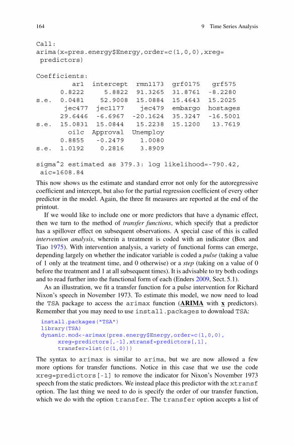
164 9 Time Series Analysis
Call:arima(x=pres.energy$Energy,order=c(1,0,0),xreg=predictors)
Coefficients:ar1 intercept rmn1173 grf0175 grf575
0.8222 5.8822 91.3265 31.8761 -8.2280s.e. 0.0481 52.9008 15.0884 15.4643 15.2025
jec477 jec1177 jec479 embargo hostages29.6446 -6.6967 -20.1624 35.3247 -16.5001
s.e. 15.0831 15.0844 15.2238 15.1200 13.7619oilc Approval Unemploy
0.8855 -0.2479 1.0080s.e. 1.0192 0.2816 3.8909
sigma^2 estimated as 379.3: log likelihood=-790.42,aic=1608.84
This now shows us the estimate and standard error not only for the autoregressivecoefficient and intercept, but also for the partial regression coefficient of every otherpredictor in the model. Again, the three fit measures are reported at the end of theprintout.
If we would like to include one or more predictors that have a dynamic effect,then we turn to the method of transfer functions, which specify that a predictorhas a spillover effect on subsequent observations. A special case of this is calledintervention analysis, wherein a treatment is coded with an indicator (Box andTiao 1975). With intervention analysis, a variety of functional forms can emerge,depending largely on whether the indicator variable is coded a pulse (taking a valueof 1 only at the treatment time, and 0 otherwise) or a step (taking on a value of 0before the treatment and 1 at all subsequent times). It is advisable to try both codingsand to read further into the functional form of each (Enders 2009, Sect. 5.1).
As an illustration, we fit a transfer function for a pulse intervention for RichardNixon’s speech in November 1973. To estimate this model, we now need to loadthe TSA package to access the arimax function (ARIMA with x predictors).Remember that you may need to use install.packages to download TSA:
install.packages("TSA")library(TSA)dynamic.mod<-arimax(pres.energy$Energy,order=c(1,0,0),
xreg=predictors[,-1],xtransf=predictors[,1],transfer=list(c(1,0)))
The syntax to arimax is similar to arima, but we are now allowed a fewmore options for transfer functions. Notice in this case that we use the codexreg=predictors[-1] to remove the indicator for Nixon’s November 1973speech from the static predictors. We instead place this predictor with the xtransfoption. The last thing we need to do is specify the order of our transfer function,which we do with the option transfer. The transfer option accepts a list of

9.1 The Box–Jenkins Method 165
vectors, one vector per transfer function predictor. For our one transfer function, wespecify c(1,0): The first term refers to the order of the dynamic decay term (so a0 here actually reverts back to a static model), and the second term refers to the laglength of the predictor’s effect (so if we expected an effect to grow, we might put ahigher number than 0 here). With these settings, we say that Nixon’s speech had aneffect in the month he gave it, and then the effect spilled over to subsequent monthsat a decaying rate.
By typing dynamic.mod, we get our output:
Call:arimax(x=pres.energy$Energy,order=c(1,0,0),xreg=predictors[,-1],
xtransf = predictors[, 1], transfer = list(c(1, 0)))
Coefficients:ar1 intercept grf0175 grf575 jec477
0.8262 20.2787 31.5282 -7.9725 29.9820s.e. 0.0476 46.6870 13.8530 13.6104 13.5013
jec1177 jec479 embargo hostages oilc-6.3304 -19.8179 25.9388 -16.9015 0.5927
s.e. 13.5011 13.6345 13.2305 12.4422 0.9205Approval Unemploy T1-AR1 T1-MA0-0.2074 0.1660 0.6087 160.6241
s.e. 0.2495 3.5472 0.0230 17.0388
sigma^2 estimated as 305.1: log likelihood=-770.83,aic=1569.66
The output is similar to that from the static ARIMA regression model, but now thereare two terms for the effect of Nixon’s speech. The first, T1-AR1, gives the decayterm. The closer this term is to 1, the more persistent the variable’s effect is. Thesecond term, T1-MA0, is the initial effect of the speech on energy coverage in themonth it was given.8 In terms of model fit, notice that the output of every ARIMA ortransfer function model we have estimated reports the Akaike information criterion(AIC). With this measure, lower scores indicate a better penalized fit. With a scoreof 1569.66, this dynamic transfer function model has the lowest AIC of any model
8In this case, we have a pulse input, so we can say that in November 1973, the effect of thespeech was an expected 161 increase in news stories, holding all else equal. In December 1973, thecarryover effect is that we expect 98 more stories, holding all else equal because 161 � 0:61 � 98.In January 1974, the effect of the intervention is we expect 60 more stories, ceteris paribus because161 � 0:61 � 0:61 � 60. The effect of the intervention continues forward in a similar decayingpattern. By contrast, if we had gotten these results with a step intervention instead of a pulseintervention, then these effects would accumulate rather than decay. Under this hypothetical, theeffects would be 161 in November 1973, 259 in December 1973 (because 161+98=259), and 319in January 1974 (because 161+98+60=319).
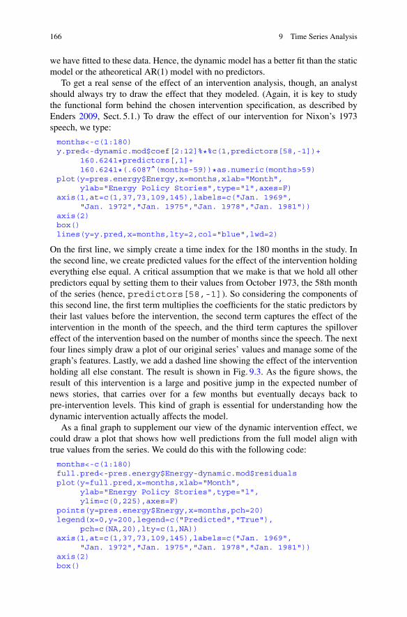
166 9 Time Series Analysis
we have fitted to these data. Hence, the dynamic model has a better fit than the staticmodel or the atheoretical AR(1) model with no predictors.
To get a real sense of the effect of an intervention analysis, though, an analystshould always try to draw the effect that they modeled. (Again, it is key to studythe functional form behind the chosen intervention specification, as described byEnders 2009, Sect. 5.1.) To draw the effect of our intervention for Nixon’s 1973speech, we type:
months<-c(1:180)y.pred<-dynamic.mod$coef[2:12]%*%c(1,predictors[58,-1])+
160.6241*predictors[,1]+160.6241*(.6087^(months-59))*as.numeric(months>59)
plot(y=pres.energy$Energy,x=months,xlab="Month",ylab="Energy Policy Stories",type="l",axes=F)
axis(1,at=c(1,37,73,109,145),labels=c("Jan. 1969","Jan. 1972","Jan. 1975","Jan. 1978","Jan. 1981"))
axis(2)box()lines(y=y.pred,x=months,lty=2,col="blue",lwd=2)
On the first line, we simply create a time index for the 180 months in the study. Inthe second line, we create predicted values for the effect of the intervention holdingeverything else equal. A critical assumption that we make is that we hold all otherpredictors equal by setting them to their values from October 1973, the 58th monthof the series (hence, predictors[58,-1]). So considering the components ofthis second line, the first term multiplies the coefficients for the static predictors bytheir last values before the intervention, the second term captures the effect of theintervention in the month of the speech, and the third term captures the spillovereffect of the intervention based on the number of months since the speech. The nextfour lines simply draw a plot of our original series’ values and manage some of thegraph’s features. Lastly, we add a dashed line showing the effect of the interventionholding all else constant. The result is shown in Fig. 9.3. As the figure shows, theresult of this intervention is a large and positive jump in the expected number ofnews stories, that carries over for a few months but eventually decays back topre-intervention levels. This kind of graph is essential for understanding how thedynamic intervention actually affects the model.
As a final graph to supplement our view of the dynamic intervention effect, wecould draw a plot that shows how well predictions from the full model align withtrue values from the series. We could do this with the following code:
months<-c(1:180)full.pred<-pres.energy$Energy-dynamic.mod$residualsplot(y=full.pred,x=months,xlab="Month",
ylab="Energy Policy Stories",type="l",ylim=c(0,225),axes=F)
points(y=pres.energy$Energy,x=months,pch=20)legend(x=0,y=200,legend=c("Predicted","True"),
pch=c(NA,20),lty=c(1,NA))axis(1,at=c(1,37,73,109,145),labels=c("Jan. 1969",
"Jan. 1972","Jan. 1975","Jan. 1978","Jan. 1981"))axis(2)box()
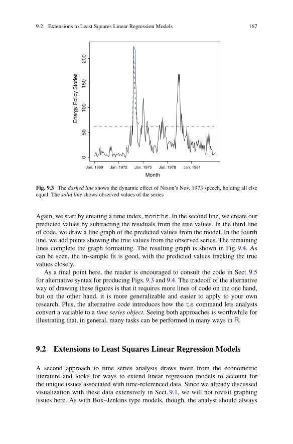
9.2 Extensions to Least Squares Linear Regression Models 167
Month
Ene
rgy
Pol
icy
Sto
ries
Jan. 1981
050
100
150
200
Jan. 1969 Jan. 1972 Jan. 1975 Jan. 1978
Fig. 9.3 The dashed line shows the dynamic effect of Nixon’s Nov. 1973 speech, holding all elseequal. The solid line shows observed values of the series
Again, we start by creating a time index, months. In the second line, we create ourpredicted values by subtracting the residuals from the true values. In the third lineof code, we draw a line graph of the predicted values from the model. In the fourthline, we add points showing the true values from the observed series. The remaininglines complete the graph formatting. The resulting graph is shown in Fig. 9.4. Ascan be seen, the in-sample fit is good, with the predicted values tracking the truevalues closely.
As a final point here, the reader is encouraged to consult the code in Sect. 9.5for alternative syntax for producing Figs. 9.3 and 9.4. The tradeoff of the alternativeway of drawing these figures is that it requires more lines of code on the one hand,but on the other hand, it is more generalizable and easier to apply to your ownresearch. Plus, the alternative code introduces how the ts command lets analystsconvert a variable to a time series object. Seeing both approaches is worthwhile forillustrating that, in general, many tasks can be performed in many ways in R.
9.2 Extensions to Least Squares Linear Regression Models
A second approach to time series analysis draws more from the econometricliterature and looks for ways to extend linear regression models to account forthe unique issues associated with time-referenced data. Since we already discussedvisualization with these data extensively in Sect. 9.1, we will not revisit graphingissues here. As with Box–Jenkins type models, though, the analyst should always

168 9 Time Series Analysis
Month
Ene
rgy
Pol
icy
Sto
ries
PredictedTrue
Jan. 1969
050
100
200
150
Jan. 1981Jan. 1972 Jan. 1975 Jan. 1978
Fig. 9.4 Predicted values from a full transfer function model on a line, with actual observed valuesas points
begin by drawing a line plot of the series of interest, and ideally a few key predictorsas well. Even diagnostic plots such as the ACF and PACF would be appropriate, inaddition to residual diagnostics such as we will discuss shortly.
When modeling data from an econometric approach, researchers again have todecide whether to use a static or a dynamic specification of the model. For staticmodels in which current values of predictors affect current values of the outcome,researchers may estimate the model with ordinary least squares (OLS) in the rarecase of no serial correlation. For efficiency gains on a static model, however, feasiblegeneralized least squares (FGLS) is a better estimator. By contrast, in the case of adynamic functional form, a lag structure can be introduced into the linear model’sspecification.
Starting with static models, the simplest kind of model (though rarely appropri-ate) would be to estimate the model using simple OLS. Returning to our energypolicy data, our model specification here would be:
static.ols<-lm(Energy~rmn1173+grf0175+grf575+jec477+jec1177+jec479+embargo+hostages+oilc+Approval+Unemploy,data=pres.energy)
By typing summary(static.ols) we get our familiar output from a linearregression model. Beware, though, that if there is serial correlation in the distur-bances, these estimates of the standard errors are incorrect:
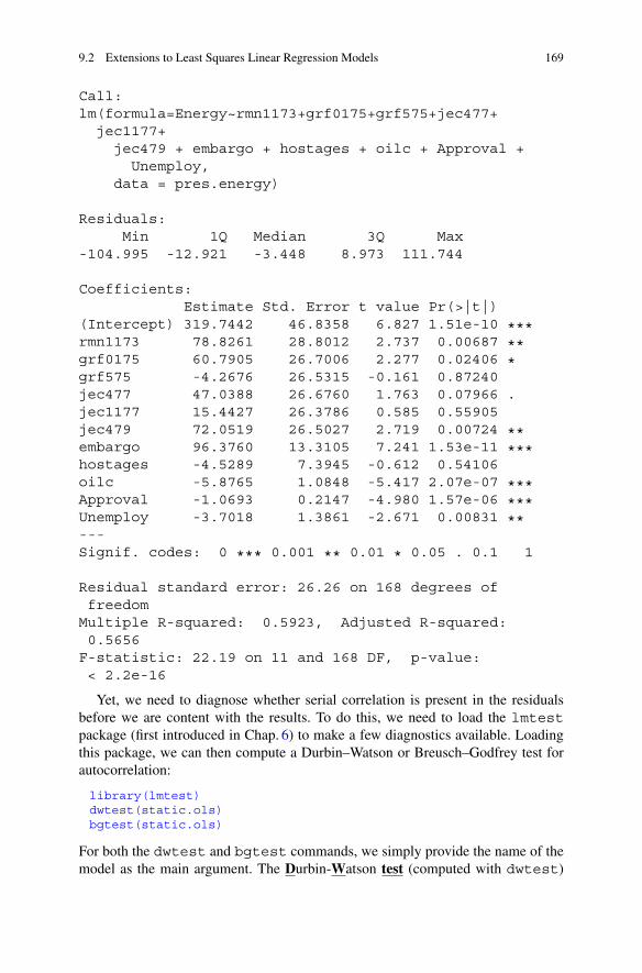
9.2 Extensions to Least Squares Linear Regression Models 169
Call:lm(formula=Energy~rmn1173+grf0175+grf575+jec477+
jec1177+jec479 + embargo + hostages + oilc + Approval +Unemploy,
data = pres.energy)
Residuals:Min 1Q Median 3Q Max
-104.995 -12.921 -3.448 8.973 111.744
Coefficients:Estimate Std. Error t value Pr(>|t|)
(Intercept) 319.7442 46.8358 6.827 1.51e-10 ***rmn1173 78.8261 28.8012 2.737 0.00687 **grf0175 60.7905 26.7006 2.277 0.02406 *grf575 -4.2676 26.5315 -0.161 0.87240jec477 47.0388 26.6760 1.763 0.07966 .jec1177 15.4427 26.3786 0.585 0.55905jec479 72.0519 26.5027 2.719 0.00724 **embargo 96.3760 13.3105 7.241 1.53e-11 ***hostages -4.5289 7.3945 -0.612 0.54106oilc -5.8765 1.0848 -5.417 2.07e-07 ***Approval -1.0693 0.2147 -4.980 1.57e-06 ***Unemploy -3.7018 1.3861 -2.671 0.00831 **---Signif. codes: 0 *** 0.001 ** 0.01 * 0.05 . 0.1 1
Residual standard error: 26.26 on 168 degrees offreedomMultiple R-squared: 0.5923, Adjusted R-squared:0.5656F-statistic: 22.19 on 11 and 168 DF, p-value:< 2.2e-16
Yet, we need to diagnose whether serial correlation is present in the residualsbefore we are content with the results. To do this, we need to load the lmtestpackage (first introduced in Chap. 6) to make a few diagnostics available. Loadingthis package, we can then compute a Durbin–Watson or Breusch–Godfrey test forautocorrelation:
library(lmtest)dwtest(static.ols)bgtest(static.ols)
For both the dwtest and bgtest commands, we simply provide the name of themodel as the main argument. The Durbin-Watson test (computed with dwtest)

170 9 Time Series Analysis
tests for first-order serial correlation and is not valid for a model that includes alagged dependent variable. Our test produces the following output:
Durbin-Watson test
data: static.olsDW = 1.1649, p-value = 1.313e-09alternative hypothesis: true autocorrelation is greater
than 0
The Durbin–Watson d statistic (1.1649 in this case), does not have a parametricdistribution. Traditionally the value of d has been checked against tables basedon Monte Carlo results to determine significance. R, however, does provide anapproximate p-value with the statistic. For a Durbin–Watson test, the null hypothesisis that there is no autocorrelation, so our significant value of d suggests thatautocorrelation is a problem.
Meanwhile, the results of our Breusch-Godfrey test (computed with bgtest)offer a similar conclusion. The Breusch–Godfrey test has a �2 distribution andcan be used to test autocorrelation in a model with a lagged dependent variable.By default, the bgtest command checks for first-order serial correlation, thoughhigher-order serial correlation can be tested with the order option. Our output inthis case is:
Breusch-Godfrey test for serial correlation oforder up to
1
data: static.olsLM test = 38.6394, df = 1, p-value = 5.098e-10
Again, the null hypothesis is that there is no autocorrelation, so our significant �2
value shows that serial correlation is a concern, and we need to do something toaccount for this.
At this point, we can draw one of two conclusions: The first possibility is thatour static model specification is correct, and we need to find an estimator that isefficient in the presence of error autocorrelation. The second possibility is that wehave overlooked a dynamic effect and need to respecify our model. (In other words,if there is a true spillover effect, and we have not modeled it, then the errors willappear to be serially correlated.) We will consider each possibility.
First, if we are confident that our static specification is correct, then our functionalform is right, but under the Gauss–Markov theorem OLS is inefficient with errorautocorrelation, and the standard errors are biased. As an alternative, we canuse feasible generalized least squares (FGLS), which estimates the level of errorcorrelation and incorporates this into the estimator. There are a variety of estimationtechniques here, including the Prais–Winsten and Cochrane–Orcutt estimators. Weproceed by illustrating the Cochrane–Orcutt estimator, though users should be wary

9.2 Extensions to Least Squares Linear Regression Models 171
of the model’s assumptions.9 In short, Cochrane–Orcutt reestimates the modelseveral times, updating the estimate of error autocorrelation each time, until itconverges to a stable estimate of the correlation. To implement this procedure inR, we need to install and then load the orcutt package:
install.packages("orcutt")library(orcutt)cochrane.orcutt(static.ols)
Once we have loaded this package, we insert the name of a linear model we haveestimated with OLS into the cochrane.orcutt command. This then iterativelyreestimates the model and produces our FGLS results as follows:
$Cochrane.Orcutt
Call:lm(formula = YB ~ XB - 1)
Residuals:Min 1Q Median 3Q Max
-58.404 -9.352 -3.658 8.451 100.524
Coefficients:Estimate Std. Error t value Pr(>|t|)
XB(Intercept) 16.8306 55.2297 0.305 0.7609XBrmn1173 91.3691 15.6119 5.853 2.5e-08 ***XBgrf0175 32.2003 16.0153 2.011 0.0460 *XBgrf575 -7.9916 15.7288 -0.508 0.6121XBjec477 29.6881 15.6159 1.901 0.0590 .XBjec1177 -6.4608 15.6174 -0.414 0.6796XBjec479 -20.0677 15.6705 -1.281 0.2021XBembargo 34.5797 15.0877 2.292 0.0232 *XBhostages -16.9183 14.1135 -1.199 0.2323XBoilc 0.8240 1.0328 0.798 0.4261XBApproval -0.2399 0.2742 -0.875 0.3829XBUnemploy -0.1332 4.3786 -0.030 0.9758---Signif. codes: 0 *** 0.001 ** 0.01 * 0.05 . 0.1 1
Residual standard error: 20.19 on 167 degrees offreedom
9In particular, at each stage of the iterative process, the linear model is estimated by regressingy�
t D yt � �yt�1 on x�t D xt � �xt�1 (Hamilton 1994, p. 223). This procedure assumes that the
dynamic adjustment process is the same for the outcome and the input variables, which is unlikely.Hence, a dynamic specification such as an autoregressive distributive lag model would be moreflexible.

172 9 Time Series Analysis
Multiple R-squared: 0.2966, Adjusted R-squared:0.2461
F-statistic: 5.87 on 12 and 167 DF, p-value:1.858e-08
$rho[1] 0.8247688
$number.interaction[1] 15
The first portion of table looks like the familiar linear regression output (though theletters XB appear before the name of each predictor). All of these coefficients, stan-dard errors, and inferential statistics have the exact same interpretation as in a modelestimated with OLS, but our estimates now should be efficient because they werecomputed with FGLS. Near the bottom of the output, we see $rho, which shows usour final estimate of error autocorrelation. We also see $number.interaction,which informs us that the model was reestimated in 15 iterations before it convergedto the final result. FGLS is intended to produce efficient estimates if a staticspecification is correct.
By contrast, if we believe a dynamic specification is correct, we need to workto respecify our linear model to capture that functional form. In fact, if we get thefunctional form wrong, our results are biased, so getting this right is critical. Addinga lag specification to our model can be made considerably easier if we install andload the dyn package. We name our model koyck.ols for reasons that will beapparent shortly:
install.packages("dyn")library(dyn)pres.energy<-ts(pres.energy)koyck.ols<-dyn$lm(Energy~lag(Energy,-1)+rmn1173+
grf0175+grf575+jec477+jec1177+jec479+embargo+hostages+oilc+Approval+Unemploy,data=pres.energy)
After loading dyn, the second line uses the ts command to declare that our data aretime series data. In the third line, notice that we changed the linear model commandto read, dyn$lm. This modification allows us to include lagged variables within ourmodel. In particular, we now have added lag(Energy,-1), which is the laggedvalue of our dependent variable. With the lag command, we specify the variablebeing lagged and how many times to lag it. By specifying -1, we are looking at theimmediately prior value. (Positive values represent future values.) The default lag is0, which just returns current values.
We can see the results of this model by typing summary(koyck.ols):
Call:lm(formula = dyn(Energy ~ lag(Energy, -1) + rmn1173 +
grf0175 +

9.2 Extensions to Least Squares Linear Regression Models 173
grf575 + jec477 + jec1177 + jec479 + embargo +hostages +
oilc + Approval + Unemploy), data = pres.energy)
Residuals:Min 1Q Median 3Q Max
-51.282 -8.638 -1.825 7.085 70.472
Coefficients:Estimate Std. Error t value Pr(>|t|)
(Intercept) 62.11485 36.96818 1.680 0.09479 .lag(Energy, -1) 0.73923 0.05113 14.458 < 2e-16 ***rmn1173 171.62701 20.14847 8.518 9.39e-15 ***grf0175 51.70224 17.72677 2.917 0.00403 **grf575 7.05534 17.61928 0.400 0.68935jec477 39.01949 17.70976 2.203 0.02895 *jec1177 -10.78300 17.59184 -0.613 0.54075jec479 28.68463 17.83063 1.609 0.10958embargo 10.54061 10.61288 0.993 0.32206hostages -2.51412 4.91156 -0.512 0.60942oilc -1.14171 0.81415 -1.402 0.16268Approval -0.15438 0.15566 -0.992 0.32278Unemploy -0.88655 0.96781 -0.916 0.36098---Signif. codes: 0 *** 0.001 ** 0.01 * 0.05 . 0.1 1
Residual standard error: 17.42 on 166 degrees offreedom(2 observations deleted due to missingness)
Multiple R-squared: 0.822, Adjusted R-squared:0.8092
F-statistic: 63.89 on 12 and 166 DF, p-value:< 2.2e-16
Our specification here is often called a Koyck model. This is because Koyck (1954)observed that when a lagged dependent variable is included as a predictor, eachpredictor will have spillover effects in subsequent months.
Consider two examples of predictor spillover effects. First, our coefficient forNixon’s speech is approximately 172. Here, we are interested in an impulse effectwhereby the predictor increased to 1 in the month the speech was given, and thenwent back to 0. Therefore, in the month of November 1973 when the speechwas given, the expected effect of this speech holding all else equal is a 172 storyincrease in energy policy coverage. However, in December 1973, November’s levelof coverage is a predictor, and November’s coverage was shaped by the speech.Since our coefficient on the lagged dependent variable is approximately 0.74, andsince 0:74 � 172 � 128, we therefore expect that the speech increased energycoverage in December by 128, ceteris paribus. Yet the effect would persist intoJanuary as well because December’s value predicts January 1974s value. Since

174 9 Time Series Analysis
0:74 � 0:74 � 172 � 94, we expect the effect of Nixon’s speech to be a 94story increase in energy coverage in January, ceteris paribus. This kind of decayingdynamic effect persists for an impulse effect in any of these variables, so this is apowerful way to specify a dynamic model. Also, bear in mind that a researcher couldeasily plot these decaying intervention effects over time to visualize the dynamicimpact of an intervention. Such a graph is valid for a Koyck model and wouldresemble the output of Fig. 9.3.
Second, consider the effect of unemployment. We should not make much ofthis predictor’s impact because the coefficient is not discernible, but it does serveas an example of interpreting a continuous predictor’s dynamic effect. If we areinterested in a step effect, we would like to know what the long-run impact wouldbe if a predictor increased by a single unit and stayed at that higher level. Soalthough it is not statistically discernible, the coefficient for unemployment is �0:89,meaning that a percentage point increase in unemployment decreases news attentionto energy policy by nearly nine-tenths of a story, in the same month, on average, andceteris paribus. But if unemployment stayed a percentage point higher, how wouldcoverage change in the long run? If ˇ13 is the coefficient on unemployment andˇ2 is the coefficient on the lagged dependent variable, then the long-term effect iscomputed by (Keele and Kelly 2006, p. 189):
ˇ13
1 � ˇ2
(9.2)
We can compute this in R simply by referencing our coefficients:
koyck.ols$coefficients[13]/(1-koyck.ols$coefficients[2])
Our output is �3:399746, which means that a persistent 1 % point rise in unem-ployment would reduce TV news coverage of energy policy in the long term by3.4 stories on average and all else equal. Again, this kind of long-term effect couldoccur for any variable that is not limited to a pulse input.
As a final strategy, we could include one or more lags of one or more predictorswithout including a lagged dependent variable. In this case, any spillover willbe limited to whatever we directly incorporate into the model specification. Forexample, if we only wanted a dynamic effect of Nixon’s speech and a staticspecification for everything else, we could specify this model:
udl.mod<-dyn$lm(Energy~rmn1173+lag(rmn1173,-1)+lag(rmn1173,-2)+lag(rmn1173,-3)+lag(rmn1173,-4)+grf0175+grf575+jec477+jec1177+jec479+embargo+hostages+oilc+Approval+Unemploy,data=pres.energy)
In this situation, we have included the current value of the Nixon’s speech indictor,as well as four lags. For an intervention, that means that this predictor will have aneffect in November 1973 and for 4 months afterwards. (In April 1974, however, theeffect abruptly drops to 0, where it stays.) We see the results of this model by typingsummary(udl.mod):
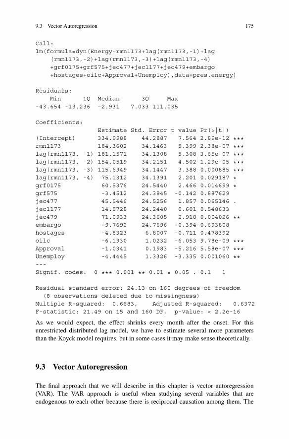
9.3 Vector Autoregression 175
Call:lm(formula=dyn(Energy~rmn1173+lag(rmn1173,-1)+lag
(rmn1173,-2)+lag(rmn1173,-3)+lag(rmn1173,-4)+grf0175+grf575+jec477+jec1177+jec479+embargo+hostages+oilc+Approval+Unemploy),data=pres.energy)
Residuals:Min 1Q Median 3Q Max
-43.654 -13.236 -2.931 7.033 111.035
Coefficients:Estimate Std. Error t value Pr(>|t|)
(Intercept) 334.9988 44.2887 7.564 2.89e-12 ***rmn1173 184.3602 34.1463 5.399 2.38e-07 ***lag(rmn1173, -1) 181.1571 34.1308 5.308 3.65e-07 ***lag(rmn1173, -2) 154.0519 34.2151 4.502 1.29e-05 ***lag(rmn1173, -3) 115.6949 34.1447 3.388 0.000885 ***lag(rmn1173, -4) 75.1312 34.1391 2.201 0.029187 *grf0175 60.5376 24.5440 2.466 0.014699 *grf575 -3.4512 24.3845 -0.142 0.887629jec477 45.5446 24.5256 1.857 0.065146 .jec1177 14.5728 24.2440 0.601 0.548633jec479 71.0933 24.3605 2.918 0.004026 **embargo -9.7692 24.7696 -0.394 0.693808hostages -4.8323 6.8007 -0.711 0.478392oilc -6.1930 1.0232 -6.053 9.78e-09 ***Approval -1.0341 0.1983 -5.216 5.58e-07 ***Unemploy -4.4445 1.3326 -3.335 0.001060 **---Signif. codes: 0 *** 0.001 ** 0.01 * 0.05 . 0.1 1
Residual standard error: 24.13 on 160 degrees of freedom(8 observations deleted due to missingness)
Multiple R-squared: 0.6683, Adjusted R-squared: 0.6372F-statistic: 21.49 on 15 and 160 DF, p-value: < 2.2e-16
As we would expect, the effect shrinks every month after the onset. For thisunrestricted distributed lag model, we have to estimate several more parametersthan the Koyck model requires, but in some cases it may make sense theoretically.
9.3 Vector Autoregression
The final approach that we will describe in this chapter is vector autoregression(VAR). The VAR approach is useful when studying several variables that areendogenous to each other because there is reciprocal causation among them. The

176 9 Time Series Analysis
basic framework is to estimate a linear regression model for each of the endogenousvariables. In each linear model, include several lagged values of the outcomevariable itself (say p lags of the variable) as well as p lags of all of the otherendogenous variables. So for the simple case of two endogenous variables, x andy, in which we set our lag length to p D 3, we would estimate two equations thatcould be represented as follows:
yt D ˇ0 C ˇ1yt�1 C ˇ2yt�2 C ˇ3yt�3 C ˇ4xt�1 C ˇ5xt�2 C ˇ6xt�3 C t (9.3)
xt D �0 C �1xt�1 C �2xt�2 C �3xt�3 C �4yt�1 C �5yt�2 C �6yt�3 C ıt
A fuller treatment on this methodology, including notation for models with moreendogenous variables and examples of models that include exogenous variables aswell, can be found in Brandt and Williams (2007). With this model, tests such asGranger causality tests can be used to assess if there is a causal effect from oneendogenous variable to another (Granger 1969).
As an example of how to implement a VAR model in R, we turn to workby Brandt and Freeman (2006), who analyze weekly data regarding the Israeli–Palestinian conflict. Their data are drawn from the Kansas Event Data System,which automatically codes English-language news reports to measure politicalevents, with a goal of using this information as an early warning to predict politicalchange. The endogenous variables in these data are scaled political actions takenby either the USA, Israel, or Palestine, and directed to one of the other actors. Thisproduces six variables a2i, a2p, i2a, p2a, i2p, and p2i. The abbreviations are “a”for American, “i” for Israeli, and “p” for Palestinian. As an example, i2p measuresthe scaled value of Israeli actions directed toward the Palestinians. The weekly datawe will use run from April 15, 1979 to October 26, 2003, for a total of 1278 weeks.
To proceed, we need to install and load the vars package to make the relevantestimation commands available. We also need the foreign package because ourdata are in Stata format:10
install.packages("vars")library(vars)library(foreign)levant.0 <- read.dta("levant.dta")levant<- subset(levant.0,
select=c("a2i","a2p","i2p","i2a","p2i","p2a"))
After loading the packages, we load our data on the third line, naming it levant.0.These data also contain three date-related indices, so for analysis purposes weactually need to create a second copy of the data that only includes our sixendogenous variables without the indices. We do this using the subset commandto create the dataset named levant.
A key step at this point is to choose the appropriate lag length, p. The laglength needs to capture all error processes and causal dynamics. One approach to
10This example requires the file levant.dta. Please download this file from the Dataverse (seepage vii) or this chapter’s online content (see page 155).

9.3 Vector Autoregression 177
determining the appropriate lag length is to fit several models, choose the modelwith the best fit, and then see if the residuals show any evidence of serial correlation.The command VARselect automatically estimates several vector autoregressionmodels and selects which lag length has the best fit. Since our data are weekly, weconsider up to 104 weeks’ lags, or 2 years’ worth of data, to consider all possibleoptions. The following command can take a minute to run because 104 models arebeing estimated:
levant.select<-VARselect(levant,type="const",lag.max=104)
To find out which of the lag lengths fits best, we can typelevant.select$ selection. Our output is simply the following:
AIC(n) HQ(n) SC(n) FPE(n)60 4 1 47
This reports the chosen lag length for the Akaike information criterion, Hannan–Quinn information criterion, Schwarz criterion, and forecast prediction error. Allfour of these indices are coded so that lower values are better. To contrast extremes,the lowest value of the Schwarz criterion, which has a heavy penalty for additionalparameters, is for the model with only one lag of the endogenous variables. Bycontrast, the best fit on the AIC comes from the model that requires 60 lags—perhaps indicating that annual seasonality is present. A much longer printoutgiving the value of each of the four fit indices for all 104 models can be seen bytyping: levant.select$criteria. Ideally, our fit indices would have settledon models with similar lag lengths. Since they did not, and since we have 1278observations, we will take the safer route with the long lag length suggested by theAIC.11
To estimate the vector autoregression model with p D 60 lags of eachendogenous variable, we type:
levant.AIC<-VAR(levant,type="const",p=60)
The VAR command requires the name of a dataset containing all of the endogenousvariables. With the type option, we have chosen "const" in this case (thedefault). This means that each of our linear models includes a constant. (Otheroptions include specifying a "trend," "both" a constant and a trend, or"none" which includes neither.) With the option p we choose the lag length.An option we do not use here is the exogen option, which allows us to specifyexogenous variables.
Once we have estimated our model using VAR, the next thing we should do isdiagnose the model using a special call to the plot function:
plot(levant.AIC,lag.acf=104,lag.pacf=104)
By using the name of our VAR model, levant.AIC, as the only argument inplot, R will automatically provide a diagnostic plot for each of the endogenous
11You are encouraged to examine the models that would have been chosen by the Hannan–Quinncriterion (4 lags) or the Schwarz criterion (1 lag) on your own. How do these models perform interms of diagnostics? How would inferences change?

178 9 Time Series Analysis
variables. With the options of lag.acf and lag.pacf, we specify that the ACFand PACF plots that this command reports should show us 2 years’ worth (104weeks) of autocorrelation patterns. For our data, R produces six plots. R displaysthese plots one at a time, and between each, the console will pose the followingprompt:
Hit <Return> to see next plot:
R will keep a plot on the viewer until you press the Return key, at which point itmoves on to the next graph. This process repeats until the graph for each outcomehas been shown.
Alternatively, if we wanted to see the diagnostic plot for one endogenous variablein particular, we could type:
plot(levant.AIC,lag.acf=104,lag.pacf=104,names="i2p")
Here, the names option has let us specify that we want to see the diagnostics for i2p(Israeli actions directed towards Palestine). The resulting diagnostic plot is shownin Fig. 9.5. The graph has four parts: At the top is a line graph that shows the truevalues in a solid black line and the fitted values in a blue dashed line. Directlybeneath this is a line plot of the residuals against a line at zero. These first twographs can illustrate whether the model consistently makes unbiased predictions ofthe outcome and whether the residuals are homoscedastic over time. In general, theforecasts consistently hover around zero, though for the last 200 observations theerror variance does seem to increase slightly. The third graph, in the bottom left,is the ACF for the residuals on i2p.12 Lastly, in the bottom right of the panel, wesee the PACF for i2p’s residuals. No spikes are significant in the ACF and only onespike is significant in the PACF over 2 years, so we conclude that our lag structurehas sufficiently filtered-out any serial correlation in this variable.
When interpreting a VAR model, we turn to two tools to draw inferencesand interpretations from these models. First, we use Granger causality testing todetermine if one endogenous variable causes the others. This test is simply a blockF-test of whether all of the lags of a variable can be excluded from the model. Fora joint test of whether one variable affects the other variables in the system, we canuse the causality command. For example, if we wanted to test whether Israeliactions towards Palestine caused actions by the other five directed dyads, we wouldtype:
causality(levant.AIC, cause="i2p")$Granger
The command here calls for the name of the model first (levant.AIC), and thenwith the cause option, we specify which of the endogenous variables we wish totest the effect of. Our output is as follows:
12Note that, by default, the graph R presents actually includes the zero-lag perfect correlation. Ifyou would like to eliminate that, given our long lag length and the size of the panel, simply loadthe TSA package before drawing the graph to change the default.

9.3 Vector Autoregression 179
−10
00−
500
0Diagram of fit and residuals for i2p
0 200 400 600 800 1000 1200
−30
0−
200
−10
00
100
0 20 40 60 80 100 0 20 40 60 80 100
−0.
06−
0.02
0.02
0.06
−0.
06−
0.02
0.02
0.06
ACF Residuals PACF Residuals
Fig. 9.5 Predicted values, residual autocorrelation function, and residual partial autocorrelationfunction for the Israel-to-Palestine series in a six-variable vector autoregression model
Granger causality H0: i2p do not Granger-causea2i a2p i2a
p2i p2a
data: VAR object levant.AICF-Test = 2.1669, df1 = 300, df2 = 5142, p-value< 2.2e-16
The null hypothesis is that the coefficients for all of the lags of i2p are zero whenmodeling each of the other five outcome variables. However, our F-test is significanthere, as the minuscule p-value shows. Therefore, we would conclude that Israeliactions directed towards Palestine do have a causal effect on the other politicalaction variables in the system.

180 9 Time Series Analysis
We can proceed to test whether each of the other five variables Granger-causethe other predictors in the system by considering each one with the causalitycommand:
causality(levant.AIC, cause="a2i")$Grangercausality(levant.AIC, cause="a2p")$Grangercausality(levant.AIC, cause="i2a")$Grangercausality(levant.AIC, cause="p2i")$Grangercausality(levant.AIC, cause="p2a")$Granger
The results are not reprinted here to preserve space. At the 95 % confidence level,though, you will see that each variable significantly causes the others, except forAmerican actions directed towards Israel (a2i).
Finally to get a sense of the substantive impact of each predictor, we turn toimpulse response analysis. The logic here is somewhat similar to the interventionanalysis we graphed back in Fig. 9.3. An impulse response function considers aone-unit increase in one of the endogenous variables and computes how such anexogenous shock would dynamically influence all of the endogenous variables,given autoregression and dependency patterns.
When interpreting an impulse response function, a key consideration is the factthat shocks to one endogenous variable are nearly always correlated with shocks toother variables. We therefore need to consider that a one-unit shock to one variable’sresidual term is likely to create contemporaneous movement in the residuals of theother variables. The off-diagonal terms of the variance–covariance matrix of theendogenous variables’ residuals, O , tells us how much the shocks covary.
There are several ways to deal with this issue. One is to use theory to determinethe ordering of the endogenous variables. In this approach, the researcher assumesthat a shock to one endogenous variable is not affected by shocks to any othervariable. Then a second variable’s shocks are affected only by the first variable’s,and no others. The researcher recursively repeats this process to identify a system inwhich all variables can be ordered in a causal chain. With a theoretically designedsystem like this, the researcher can determine how contemporaneous shocks affecteach other with a structured Cholesky decomposition of O (Enders 2009, p. 309).A second option, which is the default option in R’s irf command, is to assume thatthere is no theoretical knowledge of the causal ordering of the contemporaneousshocks and apply the method of orthogonalization of the residuals. This involvesanother Cholesky decomposition, in which we find A�1
0 by solving A�100 A0 D O .
For more details about response ordering or orthogonalizing residuals, see Brandtand Williams (2007, pp. 36–41 & 66–70), Enders (2009, pp. 307–315), or Hamilton(1994, pp. 318–324).
As an example of an impulse response function, we will graph the effect ofone extra political event from Israel directed towards Palestine. R will computeour impulse response function with the irf command, using the default orthog-onalization of residuals. One of the key options in this command is boot, whichdetermines whether to construct a confidence interval with bootstraps. Generally,it is advisable to report uncertainty in predictions, but the process can take several

9.4 Further Reading About Time Series Analysis 181
minutes.13 So if the reader wants a quick result, set boot=FALSE. To get the resultwith confidence intervals type:
levant.irf<-irf(levant.AIC,impulse="i2p",n.ahead=12,boot=TRUE)
We name our impulse response function levant.irf. The command requires usto state the name of our model (levant.AIC). The option impulse asks us toname the variable we want the effect of, the n.ahead option sets how far aheadwe wish to forecast (we say 12 weeks, or 3 months), and lastly boot determineswhether to create confidence intervals based on a bootstrap sample.
Once we have computed this, we can graph the impulse response function with aspecial call to plot:
plot(levant.irf)
The resulting graph is shown in Fig. 9.6. There are six panels, one for each ofthe six endogenous variables. The vertical axis on each panel lists the name ofthe endogenous variable and represents the expected change in that variable. Thehorizontal axis on each panel represents the number of months that have elapsedsince the shock. Each panel shows a solid red line at zero, representing where anon-effect falls on the graph. The solid black line represents the expected effectin each month, and the red dashed lines represent each confidence interval. As thefigure shows, the real impact of a shock in Israel-to-Palestine actions is dramatic tothe Israel-to-Palestine series itself (i2p) on account of autoregression and feedbackfrom effects to other series. We also see a significant jump in Palestine-to-Israelactions (p2i) over the ensuing 3 months. With the other four series, the effects palein comparison. We easily could produce plots similar to Fig. 9.6 by computing theimpulse response function for a shock in each of the six inputs. This is generally agood idea, but is omitted here for space.
9.4 Further Reading About Time Series Analysis
With these tools in hand, the reader should have some sense of how to estimate andinterpret time series models in R using three approaches—Box–Jenkins modeling,econometric modeling, and vector autoregression. Be aware that, while this chapteruses simple examples, time series analysis is generally challenging. It can bedifficult to find a good model that properly accounts for all of the trend and errorprocesses, but the analyst must carefully work through all of these issues or the
13Beware that bootstrap-based confidence intervals do not always give the correct coveragesbecause they confound information about how well the model fits with uncertainty of parameters.For this reason, Bayesian approaches are often the best way to represent uncertainty (Brandt andFreeman 2006; Sims and Zha 1999).

182 9 Time Series Analysis
a2i
010
2030
400
1020
3040
010
2030
40
010
2030
400
1020
3040
010
2030
40
a2p
i2p
i2a
p2i
0 1 2 3 4 5 6 7 8 9 10 12 0 1 2 3 4 5 6 7 8 9 10 12
p2a
Orthogonal Impulse Response from i2p
95 % Bootstrap CI, 100 runs
Fig. 9.6 Impulse response function for a one-unit shock in the Israel-to-Palestine series in a six-variable vector autoregression model
inferences will be biased. (See again, Granger and Newbold 1974.) So be sure torecognize that it often takes several tries to find a model that properly accounts forall issues.
It is also worth bearing in mind that this chapter cannot comprehensively addressany of the three approaches we consider, much less touch on all types of timeseries analysis. (Spectral analysis, wavelet analysis, state space models, and error-correction models are just a handful of topics not addressed here.) Therefore, theinterested reader is encouraged to consult other resources for further importantdetails on various topics in time series modeling. Good books that cover a rangeof time series topics and include R code are: Cowpertwait and Metcalfe (2009),Cryer and Chan (2008), and Shumway and Stoffer (2006). For more depth on

9.5 Alternative Time Series Code 183
the theory behind time series, good volumes by Political Scientists include Box-Steffensmeier et al. (2014) and Brandt and Williams (2007). Other good booksthat cover time series theory include: Box et al. 2008, Enders (2009), Wei (2006),Lütkepohl (2005), and for an advanced take see Hamilton (1994). Several booksfocus on specific topics and applying the methods in R: For instance, Petris et al.(2009) covers dynamic linear models, also called state space models, and explainshow to use the corresponding dlm package in R to apply these methods. Pfaff(2008) discusses cointegrated data models such as error-correction models andvector error-correction models, using the R package vars. Additionally, readerswho are interested in time series cross section models, or panel data, should consultthe plm package, which facilitates the estimation of models appropriate for thosemethods. Meanwhile, Mátyás and Sevestre (2008) offers a theoretical backgroundon panel data methods.
9.5 Alternative Time Series Code
As mentioned in Sect. 9.1, we will now show alternative syntax for producingFigs. 9.3 and 9.4. This code is a little longer, but is more generalizable.14 First off,if you do not have all of the packages, data objects, and models loaded from before,be sure to reload a few of them so that we can draw the figure:
library(TSA)pres.energy<-read.csv("PESenergy.csv")predictors<-as.matrix(subset(pres.energy,select=c(rmn1173,
grf0175,grf575,jec477,jec1177,jec479,embargo,hostages,oilc,Approval,Unemploy)))
All three of the previous lines of code were run earlier in the chapter. By way ofreminder, the first line loads the TSA package, the second loads our energy policycoverage data, and the third creates a matrix of predictors.
Now, to redraw either figure, we need to engage in a bit of data management:
months <- 1:180static.predictors <- predictors[,-1]dynamic.predictors <- predictors[,1, drop=FALSE]y <- ts(pres.energy$Energy, frequency=12, start=c(1972, 1))
First, we define a month index, as before. Second, we subset our matrixpredictors to those that have a static effect. Third, we isolate our dynamicpredictor of the Nixon’s speech. Fourth, we use the ts command to declare energypolicy coverage to be a time series object. On this last line, we use the frequencyoption to specify that these are monthly data (hence the value 12) and the startoption to note that these data begin in the first month of 1972.
14My thanks to Dave Armstrong for writing and suggesting this alternative code.

184 9 Time Series Analysis
Next, we need to actually estimate our transfer function. Once we have done this,we can save several outputs from the model:
dynamic.mod<-arimax(y,order=c(1,0,0),xreg=static.predictors,xtransf=dynamic.predictors,transfer=list(c(1,0)))
b <- coef(dynamic.mod)static.coefs <- b[match(colnames(static.predictors), names(b))]ma.coefs <- b[grep("MA0", names(b))]ar.coefs <- b[grep("AR1", names(b))]
The first line refits our transfer function. The second uses the coef command toextract the coefficients from the model and save them in a vector named b. The lastthree lines separate our coefficients into static effects (static.coefs), initialdynamic effects (ma.coefs), and decay terms (ar.coefs). In each line, wecarefully reference the names of our coefficient vector, using the match commandto find coefficients for the static predictors, and then the grep command to searchfor terms that contain MA0 and AR1, respectively, just as output terms of a transferfunction do.
With all of these elements extracted, we now turn specifically to redrawingFig. 9.3, which shows the effect of the Nixon’s speech intervention against the realdata. Our intervention effect consists of two parts, the expected value from holdingall of the static predictors at their values for the 58th month, and the dynamic effectof the transfer function. We create this as follows:
xreg.pred<-b["intercept"]+static.coefs%*%static.predictors[58,]transf.pred <- as.numeric(dynamic.predictors%*%ma.coefs+
ma.coefs*(ar.coefs^(months-59))*(months>59))y.pred<-ts(xreg.pred+transf.pred,frequency=12,start=c(1972,1))
The first line simply makes the static prediction from a linear equation. Thesecond uses our initial effects and decay terms to predict the dynamic effect ofthe intervention. Third, we add the two pieces together and save them as a timeseries with the same frequency and start date as the original series. With both y andy.pred now coded as time series of the same frequency over the same time span,it is now easy to recreate Fig. 9.3:
plot(y,xlab="Month", ylab="Energy Policy Stories",type="l")lines(y.pred, lty=2,col=’blue’,lwd=2)
The first line simply plots the original time series, and the second line adds theintervention effect itself.
With all of the setup work we have done, reproducing Fig. 9.4 now only requiresthree lines of code:
full.pred<-fitted(dynamic.mod)plot(full.pred,ylab="Energy Policy Stories",type="l",
ylim=c(0,225))points(y, pch=20)
The first line simply uses the fitted command to extract fitted values from thetransfer function model. The second line plots these fitted values, and the third addsthe points that represent the original series.

9.6 Practice Problems 185
9.6 Practice Problems
This set of practice problems reviews each of the three approaches to time seriesmodeling introduced in the chapter, and then poses a bonus question about thePeake and Eshbaugh-Soha energy data that asks you to learn about a new method.Questions #1–3 relate to single-equation models, so all of these questions use adataset about electricity consumption in Japan. Meanwhile, question #4 uses USeconomic data for a multiple equation model.
1. Time series visualization: Wakiyama et al. (2014) study electricity consump-tion in Japan, assessing whether the March 11, 2011, Fukushima nuclearaccident affected electricity consumption in various sectors. They do this byconducting an intervention analysis on monthly measures of electricity con-sumption in megawatts (MW), from January 2008 to December 2012. Loadthe foreign package and open these data in Stata format from the filecomprehensiveJapanEnergy.dta. This data file is available from theDataverse (see page vii) or this chapter’s online content (see page 155). We willfocus on household electricity consumption (variable name: house). Take thelogarithm of this variable and draw a line plot of logged household electricityconsumption from month-to-month. What patterns are apparent in these data?
2. Box–Jenkins modeling:
a. Plot the autocorrelation function and partial autocorrelation function forlogged household electricity consumption in Japan. What are the mostapparent features from these figures?
b. Wakiyama et al. (2014) argue that an ARIMA(1,0,1), with a SeasonalARIMA(1,0,0) component fit this series. Estimate this model and reportyour results. (Hint: For this model, you will want to include the optionseasonal=list(order=c(1,0,0), period=12) in the arimacommand.)
c. How well does this ARIMA model fit? What do the ACF and PACF look likefor the residuals from this model? What is the result of a Ljung–Box Q-test?
d. Use the arimax command from the TSA package. Estimate a model that usesthe ARIMA error process from before, the static predictors of temperature(temp) and squared temperature (temp2), and a transfer function for theFukushima intervention (dummy).
e. Bonus: The Fukushima indicator is actually a step intervention, rather thana pulse. This means that the effect cumulates rather than decays. Footnote 8describes how these effects cumulate. Draw a picture of the cumulating effectof the Fukushima intervention on logged household electricity consumption.
3. Econometric modeling:
a. Fit a static linear model using OLS for logged household electricity consump-tion in Japan. Use temperature (temp), squared temperature (temp2), andthe Fukushima indicator (dummy) as predictors. Load the lmtest package,

186 9 Time Series Analysis
and compute both a Durbin–Watson and Breusch–Godfrey test for this linearmodel. What conclusions would you draw from each? Why do you think youget this result?
b. Reestimate the static linear model of logged household electricity con-sumption using FGLS with the Cochrane–Orcutt algorithm. How similar ordifferent are your results from the OLS results? Why do you think this is?
c. Load the dyn package, and add a lagged dependent variable to this model.Which of the three econometric models do you think is the most appropriateand why? Do you think your preferred econometric model or the Box–Jenkinsintervention analysis is more appropriate? Why?
4. Vector autoregression:
a. Enders (2009, p. 315) presents quarterly data on the US economy, whichruns from the second quarter of 1959 to the first quarter of 2001. Load thevars and foreign packages, and then open the data in Stata format fromthe file moneyDem.dta. This file is available from the Dataverse (see pagevii) or this chapter’s online content (see page 155). Subset the data to onlyinclude three variables: change in logged real GDP (dlrgdp), change in thereal M2 money supply (dlrm2), and change in the 3-month interest rate onUS Treasury bills (drs). Using the VARselect command, determine thebest-fitting lag length for a VAR model of these three variables, accordingto the AIC.
b. Estimate the model you determined to be the best fit according to the AIC.Examine the diagnostic plots. Do you believe these series are clear of serialcorrelation and that the functional form is correct?
c. For each of the three variables, test whether the variable Granger-causes theother two.
d. In monetary policy, the interest rate is an important policy tool for the FederalReserve Bank. Compute an impulse response function for a percentage pointincrease in the interest rate (drs). Draw a plot of the expected changes inlogged money supply (dlrm2) and logged real GDP (dlrgdp). (Hint: Includethe option response=c("dlrgdp","dlrm2") in the irf function.)Be clear about whether you are orthogonalizing the residuals or making atheoretical assumption about response ordering.
5. Bonus: You may have noticed that Peake and Eshbaugh-Soha’s (2008) data onmonthly television coverage of the energy issue was used both as an examplefor count regression in Chap. 7 and as an example time series in this chapter.Brandt and Williams (2001) develop a Poisson autoregressive (PAR) model fortime series count data, and Fogarty and Monogan (2014) apply this model tothese energy policy data. Replicate this PAR model on these data. For replicationinformation see: http://hdl.handle.net/1902.1/16677.

Chapter 10Linear Algebra with Programming Applications
The R language has several built-in matrix algebra commands. This proves usefulfor analysts who wish to write their own estimators or have other problems inlinear algebra that they wish to compute using software. In some instances, it iseasier to apply a formula for predictions, standard errors, or some other quantitydirectly rather than searching for a canned program to compute the quantity, if oneexists. Matrix algebra makes it straightforward to compute these quantities yourself.This chapter introduces the syntax and available commands for conducting matrixalgebra in R.
The chapter proceeds by first describing how a user can input original data byhand, as a means of creating vectors, matrices, and data frames. Then it presentsseveral of the commands associated with linear algebra. Finally, we work throughan applied example in which we estimate a linear model with ordinary least squaresby programming our own estimator.
As working data throughout the chapter, we consider a simple example from the2010 US congressional election. We model the Republican candidate’s share of thetwo-party vote in elections for the House of Representatives (y) in 2010. The inputvariables are a constant (x1), Barack Obama’s share of the two-party presidentialvote in 2008 (x2), and the Republican candidate’s financial standing relative to theDemocrat in hundreds of thousands of dollars (x3). For simplicity, we model thenine House races in the state of Tennessee. The data are presented in Table 10.1.
Electronic supplementary material: The online version of this chapter(doi: 10.1007/978-3-319-23446-5_10) contains supplementary material, which is availableto authorized users.
© Springer International Publishing Switzerland 2015J.E. Monogan III, Political Analysis Using R, Use R!,DOI 10.1007/978-3-319-23446-5_10
187

188 10 Linear Algebra with Programming Applications
Table 10.1 Congressional election data from Tennessee in 2010
District Republican (y) Constant (x1) Obama (x2) Funding (x3)
1 0.808 1 0.290 4.984
2 0.817 1 0.340 5.073
3 0.568 1 0.370 12.620
4 0.571 1 0.340 �6.443
5 0.421 1 0.560 �5.758
6 0.673 1 0.370 15.603
7 0.724 1 0.340 14.148
8 0.590 1 0.430 0.502
9 0.251 1 0.770 �9.048
Note: Data from Monogan (2013a)
10.1 Creating Vectors and Matrices
As a first task, when assigning values to a vector or matrix, we must use the tra-ditional assignment command (<-). The command c combines several componentelements into a vector object.1 So to create a vector a with the specific values of 3,4, and 5:
a <- c(3,4,5)
Within c, all we need to do is separate each element of the vector with a comma.As a more interesting example, suppose we wanted to input three of the variablesfrom Table 10.1: Republican share of the two-party vote in 2010, Obama’s share ofthe two-party vote in 2008, and Republican financial advantage, all as vectors. Wewould type:
Y<-c(.808,.817,.568,.571,.421,.673,.724,.590,.251)X2<-c(.29,.34,.37,.34,.56,.37,.34,.43,.77)X3<-c(4.984,5.073,12.620,-6.443,-5.758,15.603,14.148,0.502,
-9.048)
Whenever entering data in vector form, we should generally make sure we haveentered the correct number of observations. The length command returns howmany observations are in a vector. To check all three of our vector entries, we type:
length(Y); length(X2); length(X3)
All three of our vectors should have length 9 if they were entered correctly. Observehere the use of the semicolon (;). If a user prefers to place multiple commands ona single line of text, the user can separate each command with a semicolon insteadof putting each command on a separate line. This allows simple commands to bestored more compactly.
1Alternatively, when the combined elements are complex objects, c instead creates a list object.
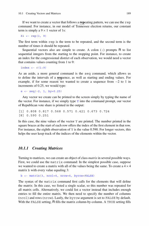
10.1 Creating Vectors and Matrices 189
If we want to create a vector that follows a repeating pattern, we can use the repcommand. For instance, in our model of Tennessee election returns, our constantterm is simply a 9 � 1 vector of 1s:
X1 <- rep(1, 9)
The first term within rep is the term to be repeated, and the second term is thenumber of times it should be repeated.
Sequential vectors also are simple to create. A colon (:) prompts R to listsequential integers from the starting to the stopping point. For instance, to createan index for the congressional district of each observation, we would need a vectorthat contains values counting from 1 to 9:
index <- c(1:9)
As an aside, a more general command is the seq command, which allows usto define the intervals of a sequence, as well as starting and ending values. Forexample, if for some reason we wanted to create a sequence from �2 to 1 inincrements of 0.25, we would type:
e <- seq(-2, 1, by=0.25)
Any vector we create can be printed to the screen simply by typing the name ofthe vector. For instance, if we simply type Y into the command prompt, our vectorof Republican vote share is printed in the output:
[1] 0.808 0.817 0.568 0.571 0.421 0.673 0.724[8] 0.590 0.251
In this case, the nine values of the vector Y are printed. The number printed in thesquare braces at the start of each row offers the index of the first element in that row.For instance, the eighth observation of Y is the value 0.590. For longer vectors, thishelps the user keep track of the indices of the elements within the vector.
10.1.1 Creating Matrices
Turning to matrices, we can create an object of class matrix in several possible ways.First, we could use the matrix command: In the simplest possible case, supposewe wanted to create a matrix with all of the values being the same. To create a 4 � 4
matrix b with every value equaling 3:
b <- matrix(3, ncol=4, nrow=4, byrow=FALSE)
The syntax of the matrix command first calls for the elements that will definethe matrix: In this case, we listed a single scalar, so this number was repeated forall matrix cells. Alternatively, we could list a vector instead that includes enoughentries to fill the entire matrix. We then need to specify the number of columns(ncol) and rows (nrow). Lastly, the byrow argument is set to FALSE by default.With the FALSE setting, R fills the matrix column-by-column. A TRUE setting fills

190 10 Linear Algebra with Programming Applications
the matrix row-by-row instead. As a rule, whenever creating a matrix, type the nameof the matrix (b in this case) into the command console to see if the way R input thedata matches what you intended.
A second simple option is to create a matrix from vectors that have already beenentered. We can bind the vectors together as column vectors using the cbindcommand and as row vectors using the rbind command. For example, in ourmodel of Tennessee election returns, we will need to create a matrix of all inputvariables in which variables define the columns and observations define the rows.Since we have defined our three variable vectors (and each vector is ordered byobservation), we can simply create such a matrix using cbind:
X<-cbind(1,X2,X3)X
The cbind command treats our vectors as columns in a matrix. This is what wewant since a predictor matrix defines rows with observations and columns withvariables. The 1 in the cbind command ensures that all elements of the first columnare equal to the constant 1. (Of course, the way we designed X1, we also could haveincluded that vector.) When typing X in the console, we get the printout:
X2 X3[1,] 1 0.29 4.984[2,] 1 0.34 5.073[3,] 1 0.37 12.620[4,] 1 0.34 -6.443[5,] 1 0.56 -5.758[6,] 1 0.37 15.603[7,] 1 0.34 14.148[8,] 1 0.43 0.502[9,] 1 0.77 -9.048
These results match the data we have in Table 10.1, so our covariate matrix shouldbe ready when we are ready to estimate our model.
Just to illustrate the rbind command, R easily would combine the vectors asrows as follows:
T<-rbind(1,X2,X3)T
We do not format data like this, but to see how the results look, typing T in theconsole results in the printout:
[,1] [,2] [,3] [,4] [,5] [,6] [,7]1.000 1.000 1.00 1.000 1.000 1.000 1.000
X2 0.290 0.340 0.37 0.340 0.560 0.370 0.340X3 4.984 5.073 12.62 -6.443 -5.758 15.603 14.148
[,8] [,9]1.000 1.000
X2 0.430 0.770X3 0.502 -9.048

10.1 Creating Vectors and Matrices 191
Hence, we see that each variable vector makes a row and each observation makes acolumn. In the printout, when R lacks the space to print an entire row on a singleline, it wraps all rows at once, thus presenting columns 8 and 9 later.
Third, we could create a matrix by using subscripting. (Additional detailson vector and matrix subscripts are presented in Sect. 10.1.3.) Sometimes whencreating a matrix, the user will know all of the values up front, but on other occasionsa user must create a matrix and then fill in the values later. In the latter case, it is agood idea to create “blanks” to fill in by designating every cell as missing (or NA).The nice feature of this is that a user can easily identify a cell that was never filled-in. By contrast, if a matrix is created with some default numeric value, say 0, thenlater on it is impossible to distinguish a cell that has a default 0 from one with a truevalue of 0. So if we wanted to create a 3 � 3 matrix named blank to fill in later, wewould write:
blank <- matrix(NA, ncol=3, nrow=3)
If we then wanted to assign the value of 8 to the first row, third column element, wewould write:
blank[1,3] <- 8
If we then wanted to insert the value � (D 3:141592 : : :) into the second row, firstcolumn entry, we would write:
blank[2,1] <- pi
If we wanted to use our previously defined vector a D .3; 4; 5/0 to define the secondcolumn, we would write:
blank[,2] <- a
We then could check our progress simply by typing blank into the commandprompt, which would print:
[,1] [,2] [,3][1,] NA 3 8[2,] 3.141593 4 NA[3,] NA 5 NA
To the left of the matrix, the row terms are defined. At the top of the matrix, thecolumn terms are defined. Notice that four elements are still coded NA because areplacement value was never offered.
Fourth, in contrast to filling-in matrices after creation, we also may know thevalues we want at the time of creating the matrix. As a simple example, to create a2 � 2 matrix W in which we list the value of each cell column-by-column:
W <- matrix(c(1,2,3,4), ncol=2, nrow=2)
Notice that our first argument is now a vector because we want to provide uniqueelements for each of the cells in the matrix. With four elements in the vector, wehave the correct number of entries for a 2 � 2 matrix. Also, in this case, we ignoredthe byrow argument because the default is to fill-in by columns. By contrast, ifwe wanted to list the cell elements row-by-row in matrix Z, we would simply setbyrow to TRUE:

192 10 Linear Algebra with Programming Applications
Z <- matrix(c(1,2,3,4), ncol=2, nrow=2, byrow=TRUE)
Type W and Z into the console and observe how the same vector of cell entries hasbeen reorganized going from one cell to another.
Alternatively, suppose we wanted to create a 10 � 10 matrix N where every cellentry was a random draw from a normal distribution with mean 10 and standarddeviation 2, or N .10; 4/:
N <- matrix(rnorm(100, mean=10, sd=2), nrow=10, ncol=10)
Because rnorm returns an object of the vector class, we are again listing a vectorto create our cell entries. The rnorm command is drawing from the normaldistribution with our specifications 100 times, which provides the number of cellentries we need for a 10 � 10 matrix.
Fifth, on many occasions, we will want to create a diagonal matrix that containsonly elements on its main diagonal (from the top left to the bottom right), with zerosin all other cells. The command diag makes it easy to create such a matrix:
D <- diag(c(1:4))
By typing D into the console, we now see how this diagonal matrix appears:
[,1] [,2] [,3] [,4][1,] 1 0 0 0[2,] 0 2 0 0[3,] 0 0 3 0[4,] 0 0 0 4
Additionally, if one inserts a square matrix into the diag command, it will return avector from the matrix’s diagonal elements. For example, in a variance-covariancematrix, the diagonal elements are variances and can be extracted quickly in this way.
10.1.2 Converting Matrices and Data Frames
A final means of creating a matrix object is with the as.matrix command. Thiscommand can take an object of the data frame class and convert it to an objectof the matrix class. For a data frame called mydata, for example, the commandmydata.2 <- as.matrix(mydata) would coerce the data into matrix form,making all of the ensuing matrix operations applicable to the data. Additionally, typ-ing mydata.3 <- as.matrix(mydata[,4:8]) would only take columnsfour through eight of the data frame and coerce those into a matrix, allowing theuser to subset the data while creating a matrix object.
Similarly, suppose we wanted to take an object of the matrix class and create anobject of the data frame class, perhaps our Tennessee electoral data from Table 10.1.In this case, the as.data.frame command will work. If we simply wanted tocreate a data frame from our covariate matrix X, we could type:
X.df <- as.data.frame(X)

10.1 Creating Vectors and Matrices 193
If we wanted to create a data frame using all of the variables from Table 10.1,including the dependent variable and index, we could type:
tennessee <- as.data.frame(cbind(index,Y,X1,X2,X3))
In this case, the cbind command embedded in as.data.frame defines amatrix, which is immediately converted to a data frame. In all, then, if a user wishesto input his or her own data into R, the most straightforward way will be to definevariable vectors, bind them together as columns, and convert the matrix to a dataframe.
10.1.3 Subscripting
As touched on in the matrix creation section, calling elements of vectors andmatrices by their subscripts can be useful for either extracting necessary informationor for making assignments. To call a specific value, we can index a vector y by thenth element, using Y[n]. So the third element of vector y, or y3, is called by:
Y[3]
To index an n � k matrix X for the value Xij, where i represents the row and jrepresents the column, use the syntax X[i,j]. If we want to select all values of thejth column of X, we can use X[,j]. For example, to return the second column ofmatrix X, type:
X[,2]
Alternatively, if a column has a name, then the name (in quotations) can be used tocall the column as well. For example:
X[,"X2"]
Similarly, if we wish to select all of the elements of the ith row of X, we can useX[i,]. For the first row of matrix X, type:
X[1,]
Alternatively, we could use a row name as well, though the matrix X does not havenames assigned to the rows.
If we wish, though, we can create row names for matrices. For example:
rownames(X)<-c("Dist. 1","Dist. 2","Dist. 3","Dist. 4","Dist. 5","Dist. 6","Dist. 7","Dist. 8","Dist. 9")
Similarly, the command colnames allows the user to define column names. Tosimply type rownames(X) or colnames(X) without making an assignment, Rwill print the row or column names saved for a matrix.
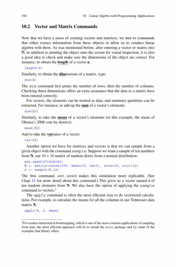
194 10 Linear Algebra with Programming Applications
10.2 Vector and Matrix Commands
Now that we have a sense of creating vectors and matrices, we turn to commandsthat either extract information from these objects or allow us to conduct linearalgebra with them. As was mentioned before, after entering a vector or matrix intoR, in addition to printing the object onto the screen for visual inspection, it is alsoa good idea to check and make sure the dimensions of the object are correct. Forinstance, to obtain the length of a vector a:
length(a)
Similarly, to obtain the dimensions of a matrix, type:
dim(X)
The dim command first prints the number of rows, then the number of columns.Checking these dimensions offers an extra assurance that the data in a matrix havebeen entered correctly.
For vectors, the elements can be treated as data, and summary quantities can beextracted. For instance, to add up the sum of a vector’s elements:
sum(X2)
Similarly, to take the mean of a vector’s elements (in this example, the mean ofObama’s 2008 vote by district):
mean(X2)
And to take the variance of a vector:
var(X2)
Another option we have for matrices and vectors is that we can sample from agiven object with the command sample. Suppose we want a sample of ten numbersfrom N, our 10 � 10 matrix of random draws from a normal distribution:
set.seed(271828183)N <- matrix(rnorm(100, mean=10, sd=2), nrow=10, ncol=10)s <- sample(N,10)
The first command, set.seed makes this simulation more replicable. (SeeChap. 11 for more detail about this command.) This gives us a vector named s often random elements from N. We also have the option of applying the samplecommand to vectors.2
The apply command is often the most efficient way to do vectorized calcula-tions. For example, to calculate the means for all the columns in our Tennessee datamatrix X:
apply(X, 2, mean)
2For readers interested in bootstrapping, which is one of the most common applications of samplingfrom data, the most efficient approach will be to install the boot package and try some of theexamples that library offers.

10.2 Vector and Matrix Commands 195
In this case, the first argument lists the matrix to analyze. The second argument, 2tells R to apply a mathematical function along the columns of the matrix. The thirdargument, mean is the function we want to apply to each column. If we wanted themean of the rows instead of the columns, we could use a 1 as the second argumentinstead of a 2. Any function defined in R can be used with the apply command.
10.2.1 Matrix Algebra
Commands that are more specific to matrix algebra are also available. Wheneverthe user wants to save the output of a vector or matrix operation, the assignmentcommand must be used. For example, if for some reason we needed the differencebetween each Republican share of the two-party vote and Obama’s share of the two-party vote, we could assign vector m to the difference of the two vectors by typing:
m <- Y - X2
With arithmetic operations, R is actually pretty flexible, but a word on how thecommands work may avoid future confusion. For addition (+) and subtraction (-): Ifthe arguments are two vectors of the same length (as is the case in computing vectorm), then R computes regular vector addition or subtraction where each element isadded to or subtracted from its corresponding element in the other vector. If thearguments are two matrices of the same size, matrix addition or subtraction applieswhere each entry is combined with its corresponding entry in the other matrix. Ifone argument is a scalar, then the scalar will be added to each element of the vectoror matrix.
Note: If two vectors of uneven length or two matrices of different size are added,an error message results, as these arguments are non-conformable. To illustrate this,if we attempted to add our sample of ten numbers from before, s, to our vector ofObama’s 2008 share of the vote, x2, as follows:
s + X2
In this case we would receive an output that we should ignore, followed by an errormessage in red:
[1] 11.743450 8.307068 11.438161 14.251645 10.828459[6] 10.336895 9.900118 10.092051 12.556688 9.775185Warning message:In s + X2 : longer object length is not a multiple of shorterobject length
This warning message tells us the output is nonsense. Since the vector s has length10, while the vector X2 has length 9, what R has done here is added the tenthelement of s to the first element of X2 and used this as the tenth element of theoutput. The error message that follows serves as a reminder that a garbage input thatbreaks the rules of linear algebra produces a garbage output that no one should use.

196 10 Linear Algebra with Programming Applications
By contrast, *, /, ^ (exponents), exp (exponential function), and log all applythe relevant operation to each scalar entry in the vector or matrix. For our matrix ofpredictors from Tennessee, for example, try the command:
X.sq <- X^2
This would return a matrix that squares each separate cell in the matrix X. Bya similar token, the simple multiplication operation (*) performs multiplicationelement by element. Hence, if two vectors are of the same length or two matricesof the same size, the output will be a vector or matrix of the same size where eachelement is the product of the corresponding elements. Just as an illustration, let usmultiply Obama’s share of the two-party vote by Republican financial advantage ina few ways. (The quantities may be silly, but this offers an example of how the codeworks.) Try for example:
x2.x3 <- X2*X3
The output vector is:
[1] 1.44536 1.72482 4.66940 -2.19062 -3.22448[6] 5.77311 4.81032 0.21586 -6.96696
This corresponds to element-by-element scalar multiplication.More often, the user actually will want to conduct proper matrix multiplication.
In R, matrix multiplication is conducted by the %*% operation. So if we had insteadmultiplied our two vectors of Obama vote share and Republican financial advantagein this way:
x2.x3.inner <- X2%*%X3
R would now return the inner product, or dot product (x2 � x3). This equals 6.25681in our example. Another useful quantity for vector multiplication is the outerproduct, or tensor product (x2 ˝ x3). We can obtain this by transposing the secondvector in our code:
x2.x3.outer <- X2%*%t(X3)
The output of this command is a 9 � 9 matrix. To obtain this quantity, the transposecommand (t) was used.3 In matrix algebra, we may need to turn row vectorsto column vectors or vice versa, and the transpose operation accomplishes this.Similarly, when applied to a matrix, every row becomes a column and every columnbecomes a row.
As one more example of matrix multiplication, the input variable matrix X hassize 9 � 3, and the matrix T that lets variables define rows is a 3 � 9 matrix. Inthis case, we could create the matrix P D TX because the number of columns ofT is the same as the number of rows of X. We therefore can say that the matricesare conformable for multiplication and will result in a matrix of size 3 � 3. We cancompute this as:
3An alternate syntax would have been X2%o%X3.

10.2 Vector and Matrix Commands 197
P <- T%*%X
Note that if our matrices are not conformable for multiplication, then R will returnan error message.4
Beyond matrix multiplication and the transpose operation, another importantquantity that is unique to matrix algebra is the determinant of a square matrix (ora matrix that has the same number of rows as columns). Our matrix P is squarebecause it has three rows and three columns. One reason to calculate the determinantis that a square matrix has an inverse only if the determinant is nonzero.5 To computethe determinant of P, we type:
det(P)
This yields a value of 691.3339. We therefore know that P has an inverse.For a square matrix that can be inverted, the inverse is a matrix that can be
multiplied by the original to produce the identity matrix. With the solve command,R will either solve for the inverse of the matrix or convey that the matrix isnoninvertible. To try this concept, type:
invP <- solve(P)invP%*%P
On the first line, we created P�1, which is the inverse of P. On the second line, wemultiply P�1P and the printout is:
X2 X31.000000e+00 -6.106227e-16 -6.394885e-14
X2 1.421085e-14 1.000000e+00 1.278977e-13X3 2.775558e-17 -2.255141e-17 1.000000e+00
This is the basic form of the identity matrix, with values of 1 along the main diagonal(running from the top left to bottom right), and values of 0 off the diagonal. Whilethe off-diagonal elements are not listed exactly as zero, this can be attributed torounding error on R’s part. The scientific notation for the second row, first columnelement for example means that the first 13 digits after the decimal place are zero,followed by a 1 in the 14th digit.
4A unique variety of matrix multiplication is called the Kronecker product (H˝L). The Kroneckerproduct has useful applications in the analysis of panel data. See the kronecker command in Rfor more information.5As another application in statistics, the likelihood function for a multivariate normal distributionalso calls on the determinant of the covariance matrix.

198 10 Linear Algebra with Programming Applications
10.3 Applied Example: Programming OLS Regression
To illustrate the various matrix algebra operations that R has available, in this sectionwe will work an applied example by computing the ordinary least squares (OLS)estimator with our own program using real data.
10.3.1 Calculating OLS by Hand
First, to motivate the background to the problem, consider the formulation of themodel and how we would estimate this by hand. Our population linear regressionmodel for vote shares in Tennessee is: y D Xˇ C u. In this model, y is a vector ofthe Republican vote share in each district, X is a matrix of predictors (includinga constant, Obama’s share of the vote in 2008, and the Republican’s financialadvantage relative the Democrat), ˇ consists of the partial coefficient for eachpredictor, and u is a vector of disturbances. We estimate O D .X0X/�1X0y, yieldingthe sample regression function Oy D X O.
To start computing by hand, we have to define X. Note that we must include avector of 1s in order to estimate an intercept term. In scalar form, our populationmodel is: yi D ˇ1x1i C ˇ2x2i C ˇ3x3i C ui, where x1i D 1 for all i. This gives us thepredictor matrix:
X D
2
66666666666664
1 0:29 4:984
1 0:34 5:073
1 0:37 12:620
1 0:34 �6:443
1 0:56 �5:758
1 0:37 15:603
1 0:34 14:148
1 0:43 0:502
1 0:77 �9:048
3
77777777777775
Next, premultiply X by its transpose:
X0X D2
641:000 1:000 1:000 1:000 1:000 1:000 1:000 1:000 1:000
0:290 0:340 0:370 0:340 0:560 0:370 0:340 0:430 0:770
4:984 5:073 12:620 �6:443 �5:758 15:603 14:148 0:502 �9:048
3
75
2
666666666666664
1 0:29 4:984
1 0:34 5:073
1 0:37 12:620
1 0:34 �6:443
1 0:56 �5:758
1 0:37 15:603
1 0:34 14:148
1 0:43 0:502
1 0:77 �9:048
3
777777777777775

10.3 Applied Example: Programming OLS Regression 199
which works out to:
X0X D2
49:00000 3:81000 31:68100
3:81000 1:79610 6:25681
31:68100 6:25681 810:24462
3
5
We also need X0y:
X0y D2
41:000 1:000 1:000 1:000 1:000 1:000 1:000 1:000 1:000
0:290 0:340 0:370 0:340 0:560 0:370 0:340 0:430 0:770
4:984 5:073 12:620 �6:443 �5:758 15:603 14:148 0:502 �9:048
3
5
2
66666666666664
0:808
0:817
0:568
0:571
0:421
0:673
0:724
0:590
0:251
3
77777777777775
which works out to:
X0y D2
45:4230
2:0943
28:0059
3
5
Inverse by Hand
The last quantity we need is the inverse of X0X. Doing this by hand, we can solveby Gauss-Jordan elimination:
ŒX0XjI� D2
49:00000 3:81000 31:68100 1:00000 0:00000 0:00000
3:81000 1:79610 6:25681 0:00000 1:00000 0:00000
31:68100 6:25681 810:24462 0:00000 0:00000 1:00000
3
5
Divide row 1 by 9:
2
41:00000 0:42333 3:52011 0:11111 0:00000 0:00000
3:81000 1:79610 6:25681 0:00000 1:00000 0:00000
31:68100 6:25681 810:24462 0:00000 0:00000 1:00000
3
5
Subtract 3.81 times row 1 from row 2:
2
41:00000 0:42333 3:52011 0:11111 0:00000 0:00000
0:00000 0:18320 �7:15481 �0:42333 1:00000 0:00000
31:68100 6:25681 810:24462 0:00000 0:00000 1:00000
3
5

200 10 Linear Algebra with Programming Applications
Subtract 31.681 times row 1 from row 3:
2
41:00000 0:42333 3:52011 0:11111 0:00000 0:00000
0:00000 0:18320 �7:15481 �0:42333 1:00000 0:00000
0:00000 �7:15481 698:72402 �3:52011 0:00000 1:00000
3
5
Divide row 2 by 0.1832:
2
41:00000 0:42333 3:52011 0:11111 0:00000 0:00000
0:00000 1:00000 �39:05464 �2:31077 5:45852 0:00000
0:00000 �7:15481 698:72402 �3:52011 0:00000 1:00000
3
5
Add 7.15481 times row 2 to row 3:
2
41:00000 0:42333 3:52011 0:11111 0:00000 0:00000
0:00000 1:00000 �39:05464 �2:31077 5:45852 0:00000
0:00000 0:00000 419:29549 �20:05323 39:05467 1:00000
3
5
Divide row 3 by 419.29549:
2
41:00000 0:42333 3:52011 0:11111 0:00000 0:00000
0:00000 1:00000 �39:05464 �2:31077 5:45852 0:00000
0:00000 0:00000 1:00000 �0:04783 0:09314 0:00239
3
5
Add 39.05464 times row 3 to row 2:
2
41:00000 0:42333 3:52011 0:11111 0:00000 0:00000
0:00000 1:00000 0:00000 �4:17859 9:09607 0:09334
0:00000 0:00000 1:00000 �0:04783 0:09314 0:00239
3
5
Subtract 3.52011 times row 3 from row 1:
2
41:00000 0:42333 0:00000 0:27946 �0:32786 �0:00841
0:00000 1:00000 0:00000 �4:17859 9:09607 0:09334
0:00000 0:00000 1:00000 �0:04783 0:09314 0:00239
3
5
Subtract .42333 times row 2 from row 1:
2
41:00000 0:00000 0:00000 2:04838 �4:17849 �0:04792
0:00000 1:00000 0:00000 �4:17859 9:09607 0:09334
0:00000 0:00000 1:00000 �0:04783 0:09314 0:00239
3
5 D ŒIj.X0X/�1�
As a slight wrinkle in these hand calculations, we can see that .X0X/�1 is a little offdue to rounding error. It should actually be a symmetric matrix.

10.3 Applied Example: Programming OLS Regression 201
Final Answer by Hand
If we postmultiply .X0X/�1 by X0y we get:
.X0X/�1X0y D2
42:04838 �4:17849 �0:04792
�4:17859 9:09607 0:09334
�0:04783 0:09314 0:00239
3
5
2
45:4230
2:0943
28:0059
3
5 D2
41:0178
�1:0018
0:0025
3
5 D O
Or in scalar form: Oyi D 1:0178 � 1:0018x2i C 0:0025x3i.
10.3.2 Writing An OLS Estimator in R
Since inverting the matrix took so many steps and even ran into some rounding error,it will be easier to have R do some of the heavy lifting for us. (As the number ofobservations or variables rises, we will find the computational assistance even morevaluable.) In order to program our own OLS estimator in R, the key commands werequire are:
• Matrix multiplication: %*%• Transpose: t• Matrix inverse: solve
Knowing this, it is easy to program an estimator for O D .X0X/�1X0y.First we must enter our variable vectors using the data from Table 10.1 and
combine the input variables into a matrix. If you have not yet entered these, type:
Y<-c(.808,.817,.568,.571,.421,.673,.724,.590,.251)X1 <- rep(1, 9)X2<-c(.29,.34,.37,.34,.56,.37,.34,.43,.77)X3<-c(4.984,5.073,12.620,-6.443,-5.758,15.603,14.148,0.502,
-9.048)X<-cbind(X1,X2,X3)
To estimate OLS with our own program, we simply need to translate the estimator.X0X/�1X0y into R syntax:
beta.hat<-solve(t(X)%*%X)%*%t(X)%*%Ybeta.hat
Breaking this down a bit: The solve command leads off because the first quantityis an inverse, .X0X/�1. Within the call to solve, the first argument must betransposed (hence the use of t) and then it is postmultiplied by the non-transposedcovariate matrix (hence the use of %*%). We follow up by postmultiplying thetranspose of X, then postmultiplying the vector of outcomes (y). When we printour results, we get:
[,1]1.017845630
X2 -1.001809341X3 0.002502538

202 10 Linear Algebra with Programming Applications
These are the same results we obtained by hand, despite the rounding discrepancieswe encountered when inverting on our own. Writing the program in R, however,simultaneously gave us full control over the estimator, while being much quickerthan the hand operations.
Of course an even faster option would be to use the canned lm command we usedin Chap. 6:
tennessee <- as.data.frame(cbind(Y,X2,X3))lm(Y~X2+X3, data=tennessee)
This also yields the exact same results. In practice, whenever computing OLSestimates, this is almost always the approach we will want to take. However, thisprocedure has allowed us to verify the usefulness of R’s matrix algebra commands.If the user finds the need to program a more complex estimator for which there isnot a canned command, this should offer relevant tools with which to accomplishthis.
10.3.3 Other Applications
With these basic tools in hand, users should now be able to begin programming withmatrices and vectors. Some intermediate applications of this include: computingstandard errors from models estimated with optim (see Chap. 11) and predictedvalues for complicated functional forms (see the code that produced Fig. 9.3). Someof the more advanced applications that can benefit from using these tools include:feasible generalized least squares (including weighted least squares), optimizinglikelihood functions for multivariate normal distributions, and generating correlateddata using Cholesky decomposition (see the chol command). Very few programsoffer the estimation and programming flexibility that R does whenever matrixalgebra is essential to the process.
10.4 Practice Problems
For these practice problems, consider the data on congressional elections in Arizonain 2010, presented below in Table 10.2:

10.4 Practice Problems 203
Table 10.2 Congressional election data from Arizona in 2010
District Republican (y) Constant (x1) Obama (x2) Funding (x3)
1 0.50 1 0.44 �9.11
2 0.65 1 0.38 8.31
3 0.52 1 0.42 8.00
4 0.28 1 0.66 �8.50
5 0.52 1 0.47 �7.17
6 0.67 1 0.38 5.10
7 0.45 1 0.57 �5.32
8 0.47 1 0.46 �18.64
Note: Data from Monogan (2013a)
1. Create a vector consisting of the Republican share of the two-party vote (y) in Arizona’s eightcongressional districts. Using any means you prefer, create a matrix, X, in which the eight rowsrepresent Arizona’s eight districts, and the three columns represent a constant vector of ones(x1), Obama’s 2008 share of the vote (x2), and the Republican’s financial balance (x3). Print outyour vector and matrix, and ask R to compute the vector’s length and matrix’s dimensions. Areall of these outputs consistent with the data you see in Table 10.2?
2. Using your matrix, X, compute X0X using R’s commands. What is your result?3. Using R’s commands, find the inverse of your previous answer. That is, compute .X0X/�1.
What is your result?4. Using the data in Table 10.2, consider the regression model yi D ˇ1x1i C ˇ2x2i C ˇ3x3i C ui.
Using R’s matrix algebra commands, compute O D .X0X/�1X0y. What are your estimates ofthe regression coefficients, O
1, O2, and O
3? How do your results compare if you compute theseusing the lm command from Chap. 6?

Chapter 11Additional Programming Tools
As the last several chapters have shown, R offers users flexibility and opportunitiesfor advanced data analysis that cannot be found in many programs. In this finalchapter, we will explore R’s programming tools, which allow the user to createcode that addresses any unique problem he or she faces.
Bear in mind that many of the tools relevant to programming have already beenintroduced earlier in the book. In Chap. 10, the tools for matrix algebra in R wereintroduced, and many programs require matrix processing. Additionally, logical(or Boolean) statements are essential to programming. R’s logical operators wereintroduced in Chap. 2, so see Table 2.1 for a reminder of what each operator’sfunction is.
The subsequent sections will introduce several other tools that are important forprogramming: probability distributions, new function definition, loops, branching,and optimization (which is particularly useful for maximum likelihood estimation).The chapter will end with two large applied examples. The first, drawing fromMonogan (2013b), introduces object-oriented programming in R and applies severalprogramming tools from this chapter to finding solutions from an insoluble gametheoretic problem. The second, drawing from Signorino (1999), offers an exampleof Monte Carlo analysis and more advanced maximum likelihood estimation in R.1
Together, the two applications should showcase how all of the programming toolscan come together to solve a complex problem.
Electronic supplementary material: The online version of this chapter(doi: 10.1007/978-3-319-23446-5_11) contains supplementary material, which is availableto authorized users.1See also: Signorino (2002) and Signorino and Yilmaz (2003).
© Springer International Publishing Switzerland 2015J.E. Monogan III, Political Analysis Using R, Use R!,DOI 10.1007/978-3-319-23446-5_11
205

206 11 Additional Programming Tools
Table 11.1 Using probability distributions in R
Prefix Usage Suffix Distribution
p Cumulative distribution function norm Normal
d Probability density function logis Logistic
q Quantile function t t
r Random draw from distribution f F
unif Uniform
pois Poisson
exp Exponential
chisq Chi-squared
binom Binomial
11.1 Probability Distributions
R allows you to use a wide variety of distributions for four purposes. For eachdistribution, R allows you to call the cumulative distribution function (CDF),probability density function (PDF), quantile function, and random draws from thedistribution. All probability distribution commands consist of a prefix and a suffix.Table 11.1 presents the four prefixes, and their usage, as well as the suffixes forsome commonly used probability distributions. Each distribution’s functions takearguments unique to that probability distribution’s parameters. To see how these arespecified, use help files (e.g., ?punif, ?pexp, or ?pnorm).2
If you wanted to know the probability that a standard normal observation will beless than 1.645, use the cumulative distribution function (CDF) command pnorm:
pnorm(1.645)
Suppose you want to draw a scalar from the standard normal distribution: to drawa � N .0; 1/, use the random draw command rnorm:
a <- rnorm(1)
To draw a vector with ten values from a �2 distribution with four degrees of freedom,use the random draw command:
c <- rchisq(10,df=4)
Recall from Chap. 10 that the sample command also allows us to simulate values,whenever we provide a vector of possible values. Hence, R offers a wide array ofdata simulation commands.
2Other distributions can be loaded through various packages. For example, another usefuldistribution is the multivariate normal. By loading the MASS library, a user can sample from themultivariate normal distribution with the mvrnorm command. Even more generally, the mvtnormpackage allows the user to compute multivariate normal and multivariate t probabilities, quantiles,random deviates, and densities.

11.2 Functions 207
Suppose we have a given probability, 0.9, and we want to know the value of a �2
distribution with four degrees of freedom at which the probability of being less thanor equal to that value is 0.9. This calls for the quantile function:
qchisq(.9,df=4)
We can calculate the probability of a certain value from the probability massfunction (PMF) for a discrete distribution. Of a Poisson distribution with intensityparameter 9, what is the probability of a count of 5?
dpois(5,lambda=9)
Although usually of less interest, for a continuous distribution, we can calculate thevalue of the probability density function (PDF) of a particular value. This has noinherent meaning, but occasionally is required. For a normal distribution with mean4 and standard deviation 2, the density at the value 1 is given by:
dnorm(1,mean=4,sd=2)
11.2 Functions
R allows you to create your own functions with the function command. Thefunction command uses the basic following syntax:
function.name <- function(INPUTS){BODY}
Notice that the function command first expects the inputs to be listed in roundparentheses, while the body of the function is listed in curly braces. As can beseen, there is little constraint in what the user chooses to put into the function, so afunction can be crafted to accomplish whatever the user would like.
For example, suppose we were interested in the equation y D 2 C 1x2 . We could
define this function easily in R. All we have to do is specify that our input variableis x and our body is the right-hand side of the equation. This will create a functionthat returns values for y. We define our function, named first.fun, as follows:
first.fun<-function(x){y<-2+x^{-2}return(y)}
Although broken-up across a few lines, this is all one big command, as the curlybraces ({}) span multiple lines. With the function command, we begin bydeclaring that x is the name of our one input, based on the fact that our equationof interest has x as the name of the input variable. Next, inside the curly braces,we assign the output y as being the exact function of x that we are interested in.As a last step before closing our curly braces, we use the return command,which tells the function what the output result is after it is called. The returncommand is useful when determining function output for a couple of reasons: First,

208 11 Additional Programming Tools
−4 −2 0 2 4
02
46
81
0
x
y
Fig. 11.1 Plot of the function y D 2 C 1x2
if we define multiple objects inside of a command, this allows us to specify whatshould be printed in the output versus what was strictly internal to the function.Second, return allows us to report a list of items as an output, if we would like.Alternatively, we could have substituted the command invisible, which worksthe same way as return, except that it does not print the output on the screen, butsimply stores the output.
With this function, if we want to know what value y takes when x D 1, we needonly type: first.fun(1). Since we used return instead of invisible, theprintout simply reads:
[1] 3
Of course, the result that y D 3 here can easily be verified by hand. Similarly, weknow that if x D 3, then y D 2 1
9. To verify this fact, we can type: first.fun(3).
R will give us the corresponding printout:
[1] 2.111111
As a final task with this function, we can plot what it looks like by inserting a vectorof x values into it. Consider the code:
my.x<-seq(-4,4,by=.01)plot(y=first.fun(my.x),x=my.x,type="l",
xlab="x",ylab="y",ylim=c(0,10))
This will produce the graph featured in Fig. 11.1.As a more complicated example, consider a function that we will use as part
of a larger exercise in Sect. 11.6. The following is an expected utility function for

11.2 Functions 209
a political party in a model of how parties will choose an issue position whencompeting in sequential elections (Monogan 2013b, Eq. (6)):
EUA.A; D/ D �f�.m1 � A/2 C .m1 � D/2 C Vg (11.1)
Cı�f�.m2 � A/2 C .m2 � D/2g
In this equation, the expected utility to a political party (party A) is the sum oftwo cumulative logistic distribution functions (the functions �), with the seconddownweighted by a discount term (0 � ı � 1). Utility depends on the positionstaken by party A and party D (A and D), a valence advantage to party A (V), andthe issue position of the median voter in the first and second election (m1 and m2).This is now a function of several variables, and it requires us to use the CDF of thelogistic distribution. To input this function in R, we type:
Quadratic.A<-function(m.1,m.2,p,delta,theta.A,theta.D){util.a<-plogis(-(m.1-theta.A)^2+
(m.1-theta.D)^2+p)+delta*plogis(-(m.2-theta.A)^2+(m.2-theta.D)^2)
return(util.a)}
The plogis command computes each relevant probability from the logistic CDF,and all of the other terms are named self-evidently from Eq. (11.1) (except that prefers to the valence term V). Although this function was more complicated, all wehad to do is make sure we named every input and copied Eq. (11.1) entirely into thebody of the function.
This more complex function, Quadratic.A, still behaves like our simplefunction. For instance, we could go ahead and supply a numeric value for everyargument of the function like this:
Quadratic.A(m.1=.7,m.2=-.1,p=.1,delta=0,theta.A=.7,theta.D=.7)
Doing so prints an output of:
[1] 0.5249792
Hence, we now know that 0.52 is the expected utility to party A when the termstake on these numeric values. In isolation, this output does not mean much. In gametheory, we are typically interested in how party A (or any player) can maximize itsutility. Hence, if we take all of the parameters as fixed at the above values, exceptwe allow party A to choose A as it sees fit, we can visualize what A’s best choiceis. The following code produces the graph seen in Fig. 11.2:
positions<-seq(-1,1,.01)util.A<-Quadratic.A(m.1=.7,m.2=-.1,p=.1,delta=0,
theta.A=positions,theta.D=.7)plot(x=positions,y=util.A,type="l",
xlab="Party A’s Position",ylab="Utility")

210 11 Additional Programming Tools
−1.0 −0.5 0.0 0.5 1.0
Party A’s Position
Par
ty A
’s E
xpec
ted
Util
ity
0.1
0.2
0.3
0.4
0.5
Fig. 11.2 Plot of an advantaged party’s expected utility over two elections contingent on issueposition
In the first line, we generate a range of positions party A may choose for A. On thesecond line, we calculate a vector of expected utilities to party A at each of the issuepositions we consider and setting the other parameters at their previously mentionedvalue. Lastly, we use the plot function to draw a line graph of these utilities.It turns out that the maximum of this function is at A D 0:7, so our previouslymentioned utility of 0.52 is the best party A can do after all.
11.3 Loops
Loops are easy to write in R and can be used to repeat calculations that are eitheridentical or vary only by a few parameters. The basic structure for a loop using thefor command is:
for (i in 1:M) {COMMANDS}
In this case, M is the number of times the commands will be executed. R alsosupports loops using the while command which follow a similar commandstructure:
j <- 1while(j < M) {
COMMANDSj <- j + 1}

11.3 Loops 211
Whether a for loop or a while loop works best can vary by situation, so theuser must use his or her own judgment when choosing a setup. In general, whileloops tend to be better for problems where you would have to do something untila criterion is met (such as a convergence criterion), and for loops are generallybetter for things you want to repeat a fixed number of times. Under either structure,R will allow a wide array of commands to be included in a loop; the user’s task ishow to manage the loop’s input and output efficiently.
As a simple demonstration of how loops work, consider an example that illus-trates the law of large numbers. To do this, we can simulate random observationsfrom the standard normal distribution (easy with the rnorm) command. Since thestandard normal has a population mean of zero, we would expect the sample meanof our simulated values to be near zero. As our sample size gets larger, the samplemean should generally be closer to the population mean of zero. A loop is perfectfor this exercise: We want to repeat the calculations of simulating from the standardnormal distribution and then taking the mean of the simulations. What differs fromiteration to iteration is that we want our sample size to increase.
We can set this up easily with the following code:
set.seed(271828183)store <- matrix(NA,1000,1)for (i in 1:1000){
a <- rnorm(i)store[i] <- mean(a)}
plot(store, type="h",ylab="Sample Mean",xlab="Number of Observations")
abline(h=0,col=’red’,lwd=2)
In the first line of this code, we call the command set.seed, in order to make oursimulation experiment replicable. When R randomly draws numbers in any way,it uses a pseudo-random number generator, which is a list of 2.1 billion numbersthat resemble random draws.3 By choosing any number from 1 to 2,147,483,647,others should be able to reproduce our results by using the same numbers in theirsimulation. Our choice of 271,828,183 was largely arbitrary. In the second line ofcode, we create a blank vector named store of length 1000. This vector is wherewe will store our output from the loop. In the next four lines of code, we define ourloop. The loop runs from 1 to 1000, with the index of each iteration being namedi. In each iteration, our sample size is simply the value of i, so the first iterationsimulates one observation, and the thousandth iteration simulates 1000 observations.Hence, the sample size increases with each pass of the loop. In each pass of theprogram, R samples from a N .0; 1/ distribution and then takes the mean of thatsample. Each mean is recorded in the ith cell of store. After the loop closes, weplot our sample means against the sample size and use abline to draw a red line
3Formally, this list makes-up draws from a standard uniform distribution, which is then convertedto whatever distribution we want using a quantile function.

212 11 Additional Programming Tools
0 200 400 600 800 1000−0.
500.
00.
51.
0
Number of Observations
Sam
ple
Mea
n
Fig. 11.3 The law of large numbers and loops in action
at the population mean of zero. The result is shown in Fig. 11.3. Indeed, our plotshows the mean of the sample converging to the true mean of zero as the samplesize increases.
Loops are necessary for many types of programs, such as if you want to do aMonte Carlo analysis. In some (but not all) cases, however, loops can be slower thanvectorized versions of commands. It may be worth trying the apply command, forinstance, if it can accomplish the same goal as a loop. Which is faster often dependson the complexity of the function and the memory overhead for calculating andstoring results. So if one approach is too slow or too complicated for your computerto handle, it may be worth trying the other.
11.4 Branching
R users have the option of executing commands conditional on a Boolean statementusing the if command. This can be handy whenever the user only wants toimplement something for certain cases, or if different data types should be treateddifferently. The basic syntax of an if statement is:
if (logical_expression) {expression_1...
}

11.4 Branching 213
In this framework, the logical_expression is some Boolean statement, andexpression_1 represents whatever commands the user would like to applywhenever the logical expression is true.
As a toy example of how this works, suppose we wanted to simulate a processin which we draw two numbers from 1 to 10 (with repeated numbers allowed). Thesample command allows us to simulate this process easily, and if we embed it in afor loop we can repeat the experiment several times (say, 100 trials). If we wantedto know in how many trials both numbers came up even, we could determine thiswith an if statement. Our code comes together like this:
even.count<-0for (i in 1:100){
a<-sample(c(1:10),2,replace=TRUE)if (sum(a%%2)==0){
even.count<-even.count+1}
}even.count
The first line creates a scalar named even.count and sets it at zero. The nextline starts the loop that gives us 100 trials. The third line creates our sample oftwo numbers from 1 to 10, and names the sample a. The fourth line defines ourif statement: We use the modulo function to find the remainder when each termin our sample is divided by two.4 If the remainder for every term is zero, then allnumbers are even and the sum is zero. In that case, we have drawn a sample in whichnumbers are even. Hence, when sum(a%%2)==0 is true, then we want to add oneto a running tally of how many samples of two even numbers we have. Thereforethe fifth line of our code adds to our tally, but only in cases that meet our condition.(Notice that a recursive assignment for even.count is acceptable. R will take theold value, add one to it, and update the value that is saved.) Try this experimentyourself. As a hint, probability theory would say that 25 % of trials will yield twoeven numbers, on average.
Users also may make if. . .else branching statements such that one set ofoperations applies whenever an expression is true, and another set of operationsapplies when the expression is false. This basic structure looks like this:
if (logical_expression) {expression_1...
} else {expression_2...
}
4Recall from Chap. 1 that the modulo function gives us the remainder from division.

214 11 Additional Programming Tools
In this case, expression_1 will only be applied in cases when the logicalexpression is true, and expression_2 will only be applied in cases when thelogical expression is false.
Finally, users have the option of branching even further. With cases for whichthe first logical expression is false, thereby calling the expressions following else,these cases can be branched again with another if. . .else statement. In fact, theprogrammer can nest as many if. . .else statements as he or she would like. Toillustrate this, consider again the case when we simulate two random numbers from1 to 10. Imagine this time we want to know not only how often we draw two evennumbers, but also how often we draw two odd numbers and how often we drawone even number and one odd. One way we could address this is by keeping threerunning tallies (below named even.count, odd.count, and split.count)and adding additional branching statements:
even.count<-0odd.count<-0split.count<-0for (i in 1:100){
a<-sample(c(1:10),2,replace=TRUE)if (sum(a%%2)==0){
even.count<-even.count+1} else if (sum(a%%2)==2){
odd.count<-odd.count+1} else{
split.count<-split.count+1}
}even.countodd.countsplit.count
Our for loop starts the same as before, but after our first if statement, we followwith an else statement. Any sample that did not consist of two even numbers isnow subject to the commands under else, and the first command under elseis. . . another if statement. This next if statement observes that if both terms in thesample are odd, then the sum of the remainders after dividing by two will be two.Hence, all samples with two odd entries now are subject to the commands of thisnew if statement, where we see that our odd.count index will be increased byone. Lastly, we have a final else statement—all samples that did not consist of twoeven or two odd numbers will now be subject to this final set of commands. Sincethese samples consist of one even and one odd number, the split.count indexwill be increased by one. Try this out yourself. Again, as a hint, probability theoryindicates that on average 50 % of samples should consist of one even and one oddnumber, 25 % should consist of two even numbers, and 25 % should consist of twoodd numbers.
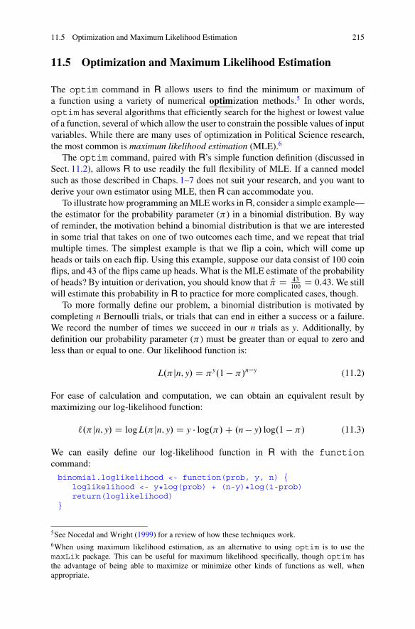
11.5 Optimization and Maximum Likelihood Estimation 215
11.5 Optimization and Maximum Likelihood Estimation
The optim command in R allows users to find the minimum or maximum ofa function using a variety of numerical optimization methods.5 In other words,optim has several algorithms that efficiently search for the highest or lowest valueof a function, several of which allow the user to constrain the possible values of inputvariables. While there are many uses of optimization in Political Science research,the most common is maximum likelihood estimation (MLE).6
The optim command, paired with R’s simple function definition (discussed inSect. 11.2), allows R to use readily the full flexibility of MLE. If a canned modelsuch as those described in Chaps. 1–7 does not suit your research, and you want toderive your own estimator using MLE, then R can accommodate you.
To illustrate how programming an MLE works in R, consider a simple example—the estimator for the probability parameter (�) in a binomial distribution. By wayof reminder, the motivation behind a binomial distribution is that we are interestedin some trial that takes on one of two outcomes each time, and we repeat that trialmultiple times. The simplest example is that we flip a coin, which will come upheads or tails on each flip. Using this example, suppose our data consist of 100 coinflips, and 43 of the flips came up heads. What is the MLE estimate of the probabilityof heads? By intuition or derivation, you should know that O� D 43
100D 0:43. We still
will estimate this probability in R to practice for more complicated cases, though.To more formally define our problem, a binomial distribution is motivated by
completing n Bernoulli trials, or trials that can end in either a success or a failure.We record the number of times we succeed in our n trials as y. Additionally, bydefinition our probability parameter (�) must be greater than or equal to zero andless than or equal to one. Our likelihood function is:
L.�jn; y/ D �y.1 � �/n�y (11.2)
For ease of calculation and computation, we can obtain an equivalent result bymaximizing our log-likelihood function:
`.�jn; y/ D log L.�jn; y/ D y � log.�/ C .n � y/ log.1 � �/ (11.3)
We can easily define our log-likelihood function in R with the functioncommand:
binomial.loglikelihood <- function(prob, y, n) {loglikelihood <- y*log(prob) + (n-y)*log(1-prob)return(loglikelihood)
}
5See Nocedal and Wright (1999) for a review of how these techniques work.6When using maximum likelihood estimation, as an alternative to using optim is to use themaxLik package. This can be useful for maximum likelihood specifically, though optim hasthe advantage of being able to maximize or minimize other kinds of functions as well, whenappropriate.

216 11 Additional Programming Tools
Now to estimate O� , we need R to find the value of � that maximizes the log-likelihood function given the data. (We call this term prob in the code to avoidconfusion with R’s use of the command pi to store the geometric constant.) We cando this with the optim command. We compute:
test <- optim(c(.5), # starting value for probbinomial.loglikelihood, # the log-likelihood functionmethod="BFGS", # optimization methodhessian=TRUE, # return numerical Hessiancontrol=list(fnscale=-1), # maximize instead of minimizey=43, n=100) # the data
print(test)
Remember that everything after a pound sign (#) is a comment that R ignores,so these notes serve to describe each line of code. We always start with a vectorof starting values with all parameters to estimate (just � in this case), name thelog-likelihood function we defined elsewhere, choose our optimization method(Broyden-Fletcher-Goldfarb-Shanno is often a good choice), and indicate that wewant R to return the numerical Hessian so we can compute standard errors later.The fifth line of code is vitally important: By default optim is a minimizer, so wehave to specify fnscale=-1 to make it a maximizer. Any time you use optimfor maximum likelihood estimation, this line will have to be included. On the sixthline, we list our data. Often, we will call a matrix or data frame here, but in this casewe need only list the values of y and n.
Our output from print(test) looks like the following:
$par[1] 0.4300015
$value[1] -68.33149
$countsfunction gradient
13 4
$convergence[1] 0
$messageNULL
$hessian[,1]
[1,] -407.9996

11.6 Object-Oriented Programming 217
To interpret our output: The par term lists the estimates of the parameters, so ourestimate is O� D 0:43 (as we anticipated). The log-likelihood for our final solutionis �68:33149, and is presented under value. The term counts tells us how oftenoptim had to call the function and the gradient. The term convergence willbe coded 0 if the optimization was successfully completed; any other value is anerror code. The message item may return other necessary information from theoptimizer. Lastly, the hessian is our matrix of second derivatives of the log-likelihood function. With only one parameter here, it is a simple 1 � 1 matrix. Ingeneral, if the user wants standard errors from an estimated maximum likelihoodmodel, the following line will return them:
sqrt(diag(solve(-test$hessian)))
This line is based on the formula for standard errors in maximum likelihoodestimation. All the user will ever need to change is to replace the word test withthe name associated with the call to optim. In this case, R reports that the standarderror is SE. O�/ D 0:0495074.
Finally, in this case in which we have a single parameter of interest, we havethe option of using our defined log-likelihood function to draw a picture of theoptimization problem. Consider the following code:
ruler <- seq(0,1,0.01)loglikelihood <- binomial.loglikelihood(ruler, y=43, n=100)plot(ruler, loglikelihood, type="l", lwd=2, col="blue",
xlab=expression(pi),ylab="Log-Likelihood",ylim=c(-300,-70),main="Log-Likelihood for Binomial Model")
abline(v=.43)
The first line defines all values that � possibly can take. The second line inserts intothe log-likelihood function the vector of possible values of � , plus the true values ofy and n. The third through fifth lines are a call to plot that gives us a line graph ofthe log-likelihood function. The last line draws a vertical line at our estimated valuefor O� . The result of this is shown in Fig. 11.4. While log-likelihood functions withmany parameters usually cannot be visualized, this does remind us that the functionwe have defined can still be used for purposes other than optimization, if need be.
11.6 Object-Oriented Programming
This section takes a turn towards the advanced, by presenting an application inobject-oriented programming. While this application does synthesize many of theother tools discussed in this chapter, novice users are less likely to use object-oriented programming than the features discussed so far. That said, for advanceduses object-oriented work can be beneficial.

218 11 Additional Programming Tools
0.0 0.2 0.4 0.6 0.8 1.0
−30
0−
250
−20
0−
150
−10
0
Log−Likelihood for Binomial Model
π
Log−
Like
lihoo
d
Fig. 11.4 Binomial log-likelihood across all possible values of probability parameter � when thedata consist of 43 successes in 100 trials
As was mentioned in Chap. 1, R is an object-oriented environment. This meansthat you, as a researcher, have the opportunity to use sophisticated programmingtools in your own research. In object-oriented programming, you create a class ofitem that has a variety of features. You then can create items within the class (calledobjects or variables) that will have unique features. In R, you can create classesfrom the object systems S3 or S4.
To illustrate, a “linear model” is a class of objects created by the lm command. Itis an S3 class. Back in Chap. 6, we estimated a model that we named mod.hours,which was an object of the linear model class. This object had features includingcoefficients, residuals, and cov.unscaled. In all S3-class objects,we can call a feature by writing the object name, the dollar sign, and the nameof the feature we want. For example, mod.hours$coefficients would listthe vector of coefficients from that model. (S4 uses slightly different referencing,described later.) When you define your own objects, you may use either S3 or S4object system. The following example saves our outputs in the S3 object system,though footnotes illustrate how you could use the S4 object system if you preferred.

11.6 Object-Oriented Programming 219
11.6.1 Simulating a Game
As a working example of object-oriented programming, we consider a somewhatsimplified version of the work presented in Monogan (2013b).7 We touched on thismodel in Sect. 11.2, introducing one actor’s utility function. In brief, this articledevelops a game theoretic model of how two parties will choose a position onan issue according to the spatial proximity model of politics. The spatial model,described somewhat in Chap. 7, assumes that issue positions can be represented aslocations in space. Voters choose parties that take issue positions closer to their ownposition in issue space, so parties try to maximize votes by strategically choosingtheir issue positions.
In the game we consider, the substantive motivation is the fact that public opinionshows strong trends on certain policy issues because of demographic trends orgenerational differences. Issues like this include environmental policy, immigrationpolicy, and protections for gay rights. We assume that two parties will compete intwo elections. However, to consider the fact that parties should be mindful of thefuture and may be held to account for past issue positions, the position they take inthe first election is the position they are stuck with in the second election. We alsoassume that the issue position of the median voter changes from one election to thenext in a way that parties anticipate, since on these issues public opinion trends areoften clear.
Another feature is that one party has an advantage in the first election (dueto incumbency or some other factor), so for this reason the players are party A(a party with a non-issue valence advantage in the first election) and party D(a disadvantaged party). The second election is assumed to be less valuable thanthe first, because the reward is farther away. Finally, voters also consider factorsunknown to the parties, so the outcome of the election is probabilistic rather thancertain. In this game, then, parties try to maximize their probability of winning eachof the two elections. How do they position themselves on an issue with changingpublic opinion?
The tricky feature of this game is that it cannot be solved algebraically (Monogan2013b, p. 288). Hence, we turn to R to help us find solutions through simulation.The first thing we need to do is clean up and define the expected utility functions forparties A and D:
rm(list=ls())Quadratic.A<-function(m.1,m.2,p,delta,theta.A,theta.D){
util.a<-plogis(-(m.1-theta.A)^2+(m.1-theta.D)^2+p)+
delta*plogis(-(m.2-theta.A)^2+
7To see the full original version of the program, consult http://hdl.handle.net/1902.1/16781. Notethat here we use the S3 object family, but the original code uses the S4 family. The originalprogram also considers alternative voter utility functions besides the quadratic proximity functionlisted here, such as an absolute proximity function and the directional model of voter utility(Rabinowitz and Macdonald 1989).

220 11 Additional Programming Tools
(m.2-theta.D)^2)return(util.a)}
Quadratic.D<-function(m.1,m.2,p,delta,theta.A,theta.D){util.d<-(1-plogis(-(m.1-theta.A)^2+
(m.1-theta.D)^2+p))+delta*(1-plogis(-(m.2-theta.A)^2+(m.2-theta.D)^2))
return(util.d)}
We already considered the function Quadratic.A in Sect. 11.2, and it is formallydefined by Eq. (11.1). Quadratic.D is similar in structure, but yields differingutilities. Both of these functions will be used in the simulations we do.
Our next step is to define a long function that uses our utility functions to run asimulation and produces an output formatted the way we want.8 All of the followingcode is one big function definition. Comments after pound signs (#) again areincluded to help distinguish each party of the function body. The function, calledsimulate, simulates our game of interest and saves our results in an object ofclass game.simulation:
simulate<-function(v,delta,m.2,m.1=0.7,theta=seq(-1,1,.1)){
#define internal parameters, matrices, and vectorsprecision<-length(theta)outcomeA<-matrix(NA,precision,precision)outcomeD<-matrix(NA,precision,precision)bestResponseA<-rep(NA,precision)bestResponseD<-rep(NA,precision)equilibriumA<- ’NA’equilibriumD<- ’NA’
#matrix attributesrownames(outcomeA)<-colnames(outcomeA)<-rownames(outcomeD)<-
colnames(outcomeD)<-names(bestResponseA)<-names(bestResponseD)<-theta
#fill-in the utilities for all strategies for party Afor (i in 1:precision){
for (j in 1:precision){outcomeA[i,j]<-Quadratic.A(m.1,m.2,v,delta,
theta[i],theta[j])}
8If you preferred to use the S4 object system for this exercise instead, the next thing wewould need to do is define the object class before defining the function. If we wantedto call our object class simulation, we would type: setClass("simulation",representation(outcomeA="matrix", outcomeD="matrix",bestResponseA="numeric", bestResponseD="numeric",equilibriumA="character", equilibriumD="character")). The S3 objectsystem does not require this step, as we will see when we create objects of our self-definedgame.simulation class.

11.6 Object-Oriented Programming 221
}
#utilities for party Dfor (i in 1:precision){
for (j in 1:precision){outcomeD[i,j]<-Quadratic.D(m.1,m.2,v,delta,
theta[i],theta[j])}
}
#best responses for party Afor (i in 1:precision){
bestResponseA[i]<-which.max(outcomeA[,i])}
#best responses for party Dfor (i in 1:precision){
bestResponseD[i]<-which.max(outcomeD[i,])}
#find the equilibriafor (i in 1:precision){
if (bestResponseD[bestResponseA[i]]==i){equilibriumA<-dimnames(outcomeA)[[1]][
bestResponseA[i]]equilibriumD<-dimnames(outcomeD)[[2]][
bestResponseD[bestResponseA[i]]]}
}
#save the outputresult<-list(outcomeA=outcomeA,outcomeD=outcomeD,
bestResponseA=bestResponseA,bestResponseD=bestResponseD,equilibriumA=equilibriumA,equilibriumD=equilibriumD)
class(result)<-"game.simulation"invisible(result)
}
As a general tip, when writing a long function, it is best to test code outsideof the function wrapper. For bonus points and to get a full sense of this code,you may want to break this function into its components and see how each pieceworks. As the comments throughout show, each set of commands does somethingwe normally might do in a function. Notice that when the arguments are defined,both m.1 and theta are given default values. This means that in future uses, if wedo not specify the values of these inputs, the function will use these defaults, but ifwe do specify them, then the defaults will be overridden. Turning to the argumentswithin the function, it starts off by defining internal parameters and setting theirattributes. Every set of commands thereafter is a loop within a loop to repeat certaincommands and fill output vectors and matrices.
The key addition here that is unique to anything discussed before is in thedefinition of the result term at the end of the function. Notice that in doing this,

222 11 Additional Programming Tools
we first define the output as a list, in which each component is named. In thiscase, we already named our objects the same as the way we want to label themin the output list, but that may not always be the case.9 We then use the classcommand to declare that our output is of the game.simulation class, a conceptwe are now creating. The class command formats this as an object in the S3family. By typing invisible(result) at the end of the function, we know thatour function will return this game.simulation-class object.10
Now that this function is defined, we can put it to use. Referring to the termsin Eq. (11.1), suppose that V D 0:1, ı D 0, m1 D 0:7, and m2 D �0:1. In thecode below, we create a new object called treatment.1 using the simulatefunction when the parameters take these values, and then we ask R to print theoutput:
treatment.1<-simulate(v=0.1,delta=0.0,m.2=-0.1)treatment.1
Notice that we did not specify m.1 because 0.7 already is the default value forthat parameter. The output from the printout of treatment.1 is too lengthy toreproduce here, but on your own screen you will see that treatment.1 is anobject of the game.simulation class, and the printout reports the values foreach attribute.
If we are only interested in a particular feature from this result, we can ask R toreturn only the value of a specific slot. For an S3 object, which is how we saved ourresult, we can call an attribute by naming the object, using the $ symbol, and thennaming the attribute we want to use. (This contrasts from S4 objects, which use the@ symbol to call slots.) For example, if we only wanted to see what the equilibriumchoices for parties A and D were, we could simply type:
treatment.1$equilibriumAtreatment.1$equilibriumD
Each of these commands returns the same output:
[1] "0.7"
So, substantively, we can conclude that the equilibrium for the game under theseparameters is A D D D 0:7, which is the ideal point of the median voter in the first
9For example, in the phrase outcomeA=outcomeA, the term to the left of the equals sign statesthat this term in the list will be named outcomeA, and the term to the right calls the object of thisname from the function to fill this spot.10The code would differ slightly for the S4 object system. If we defined our simulationclass as the earlier footnote describes, here we would replace the definition ofresult as follows: result<-new("simulation",outcomeA=outcomeA,outcomeD=outcomeD,bestResponseA=bestResponseA,bestResponseD=bestResponseD, equilibriumA=equilibriumA,equilibriumD=equilibriumD). Replacing the list command with the new commandassigns the output to our simulation class and fills the various slots all in one step. This meanswe can skip the extra step of using the class command, which we needed when using the S3system.

11.7 Monte Carlo Analysis: An Applied Example 223
election. Substantively, this should make sense because setting ı D 0 is a specialcase when the parties are not at all concerned about winning the second election, sothey position themselves strictly for the first election.11
To draw a contrast, what if we conducted a second simulation, but this timeincreased the value of ı to 0.1? We also could use finer-grained values of thepositions parties could take, establishing their position out to the hundredths decimalplace, rather than tenths. We could do this as follows:
treatment.2<-simulate(v=0.1,delta=0.1,m.2=-0.1,theta=seq(-1,1,.01))
treatment.2$equilibriumAtreatment.2$equilibriumD
We accomplished the finer precision by substituting our own vector in for theta.Our output values of the two equilibrium slots are again the same:
[1] "0.63"
So we know under this second treatment, the equilibrium for the game is A D D D0:63. Substantively, what happened here is we increased the value of winning thesecond election to the parties. As a result, the parties moved their issue position alittle closer to the median voter’s issue preference in the second election.
11.7 Monte Carlo Analysis: An Applied Example
As an applied example that synthesizes several of the tools developed in thischapter, we now conduct a Monte Carlo analysis. The basic logic of Monte Carloanalysis is that the researcher generates data knowing the true population model.The researcher then asks whether a certain method’s sample estimates have goodproperties, given what the population quantities are. Common treatments in aMonte Carlo experiment include: choice of estimator, sample size, distribution ofpredictors, variance of errors, and whether the model has the right functional form(e.g., ignoring a nonlinear relationship or omitting a predictor). By trying varioustreatments, a user can get a comparative sense of how well an estimator works.
In this case, we will introduce Signorino’s (1999) strategic multinomial probitmodel as the estimator we will use in our Monte Carlo experiment. The idea behindthis approach is that, when a recurring political situation can be represented witha game (such as militarized international disputes), we can develop an empiricalmodel of the outcomes that can occur (such as war) based on the strategy of thegame. Each possible outcome has a utility function for each player, whether theplayer be an individual, a country, or another actor. The utility represents how much
11If we had instead saved treatment.1 as an S4 simulation object as theprior footnotes described, the command to call a specific attribute would instead be:treatment.1@equilibriumA.

224 11 Additional Programming Tools
U1(∼A)+
U1(SQ)
α1∼A
U2(∼D)+ α2∼D U2(D)+α2D
U1(C), U2(C) U1(W), U2(W)
U1(A) + α1A
1
2
Fig. 11.5 Strategic deterrence model
benefit the player gets from the outcome. In this setup, we use observable predictorsto model the utilities for each possible outcome. This kind of model is interestingbecause the population data-generating process typically has nonlinearities in it thatare not captured by standard approaches. Hence, we will have to program our ownlikelihood function and use optim to estimate it.12
To motivate how the strategic multinomial probit is set up, consider a substantivemodel of behavior between two nations, an aggressor (1) and a target (2). Thisis a two-stage game: First, the aggressor decides whether to attack (A) or not(�A); then, the target decides whether to defend (D) or not (�D). Three observableconsequences could occur: if the aggressor decides not to attack, the status quoholds; if the aggressor attacks, the target may choose to capitulate; finally, ifthe target defends, we have war. The game tree is presented in Fig. 11.5. At theend of each branch are the utilities to players (1) and (2) for status quo (SQ),capitulation (C), and war (W), respectively. We make the assumption that theseplayers are rational and therefore choose the actions that maximize the resultingpayoff. For example, if the target is weak, the payoff of war U2.W/ would be terriblynegative, and probably lower than the payoff for capitulation U2.C/. If the aggressorknows this, it can deduce that in the case of attack, the target would capitulate. Theaggressor therefore would know that if it chooses to attack, it will receive the payoffU1.C/ (and not U1.W/). If the payoff of capitulation U1.C/ is bigger than the payoffof the status quo U1.SQ/ for the aggressor, the rational decision is to attack (and thetarget’s rational decision is to capitulate). Of course, the goal is to get a sense ofwhat will happen as circumstances change across different dyads of nations.
In general, we assume the utility functions respond to observable specificcircumstances (the value of the disputed resources, the expected diplomatic pricedue to sanctions in case of aggression, the military might, and so forth). We
12Readers interested in doing research like this in their own work should read about the gamespackage, which was developed to estimate this kind of model.

11.7 Monte Carlo Analysis: An Applied Example 225
will also assume that the utilities for each country’s choice are stochastic. Thisintroduces uncertainty into our payoff model, representing the fact that this model isincomplete, and probably excludes some relevant parameters from the evaluation. Inthis exercise, we will consider only four predictors Xi to model the utility functions,and assume that the payoffs are linear in these variables.
In particular, we consider the following parametric form for the payoffs:
U1.SQ/ D 0
U1.C/ D X1ˇ1
U1.W/ D X2ˇ2 (11.4)
U2.C/ D 0
U2.W/ D X3ˇ3 C X4ˇ4
˛ � N .0; 0:5/
Each nation makes its choice based on which decision will give it a bigger utility.This is based on the known information, plus an unknown private disturbance (˛) foreach choice. This private disturbance adds a random element to actors’ decisions.We as researchers can look at past conflicts, measure the predictors (X), observethe outcome, and would like to infer: How important are X1, X2, X3, and X4 in thebehavior of nation-dyads? We have to determine this based on whether each datapoint resulted in status quo, capitulation, or war.
11.7.1 Strategic Deterrence Log-Likelihood Function
We can determine estimates of each O using maximum likelihood estimation. First,we have to determine the probability (p) the target (2) will defend if attacked:
p D P.D/ D P.U2.D/ C ˛2D > U2.� D/ C ˛2�D/
D P.U2.D/ � U2.� D/ > ˛2�D � ˛2D/ (11.5)
D ˚.X3ˇ3 C X4ˇ4/
Where ˚ is the cumulative distribution function for a standard normal distribution.If we know p, we can determine the probability (q) that the aggressor (1) will attack:
q D P.A/ D P.U1.A/ C ˛1A > Ua.� A/ C ˛1�A/
D P.U1.A/ � U1.� A/ > ˛1�A � ˛1A/ (11.6)
D ˚.pX2ˇ2 C .1 � p/X1ˇ1/
Notice that p is in the equation for q. This nonlinear feature of the model is notaccommodated by standard canned models.

226 11 Additional Programming Tools
Knowing the formulae for p and q, we know the probabilities of status quo,capitulation, and war. Therefore, the likelihood function is simply the product ofthe probabilities of each event, raised to a dummy of whether the event happened,multiplied across all observations:
L.ˇjy; X/ DnY
iD1
.1 � q/DSQ � .q.1 � p//DC � .pq/DW (11.7)
Where DSQ, DC, and DW are dummy variables equal to 1 if the case is status quo,capitulation, or war, respectively, and 0 otherwise. The log-likelihood function is:
`.ˇjy; X/ DnX
iD1
DSQ log.1 � q/ C DC log q.1 � p/ C DW log.pq/ (11.8)
We are now ready to begin programming this into R. We begin by cleaning up andthen defining our log-likelihood function as llik, which again includes commentsto describe parts of the function’s body:
rm(list=ls())
llik=function(B,X,Y) {#Separate data matrices to individual variables:sq=as.matrix(Y[,1])cap=as.matrix(Y[,2])war=as.matrix(Y[,3])X13=as.matrix(X[,1])X14=as.matrix(X[,2])X24=as.matrix(X[,3:4])
#Separate coefficients for each equation:B13=as.matrix(B[1])B14=as.matrix(B[2])B24=as.matrix(B[3:4])
#Define utilities as variables times coefficients:U13=X13 %*% B13U14=X14 %*% B14U24=X24 %*% B24
#Compute probability 2 will fight (P4) or not (P3):P4=pnorm(U24)P3=1-P4
#Compute probability 1 will attack (P2) or not (P1):P2=pnorm((P3*U13+P4*U14))P1=1-P2
#Define and return log-likelihood function:lnpsq=log(P1)lnpcap=log(P2*P3)

11.7 Monte Carlo Analysis: An Applied Example 227
lnpwar=log(P2*P4)llik=sq*lnpsq+cap*lnpcap+war*lnpwarreturn(sum(llik))
}
While substantially longer than the likelihood function we defined in Sect. 11.5, theidea is the same. The function still accepts parameter values, independent variables,and dependent variables, and it still returns a log-likelihood value. With a morecomplex model, though, the function needs to be broken into component steps.First, our data are now matrices, so the first batch of code separates the variablesby equation from the model. Second, our parameters are all coefficients stored inthe argument B, so we need to separate the coefficients by equation from the model.Third, we matrix multiply the variables by the coefficients to create the three utilityterms. Fourth, we use that information to compute the probabilities that the targetwill defend or not. Fifth, we use the utilities, plus the probability of the target’sactions, to determine the probability the aggressor will attack or not. Lastly, theprobabilities of all outcomes are used to create the log-likelihood function.
11.7.2 Evaluating the Estimator
Now that we have defined our likelihood function, we can use it to simulate data andfit the model over our simulated data. With any Monte Carlo experiment, we needto start by defining the number of experiments we will run for a given treatmentand the number of simulated data points in each experiment. We also need to defineempty spaces for the outputs of each experiment. We type:
set.seed(3141593)i<-100 #number of experimentsn<-1000 #number of cases per experimentbeta.qre<-matrix(NA,i,4)stder.qre<-matrix(NA,i,4)
We start by using set.seed to make our Monte Carlo results more replicable.Here we let i be our number of experiments, which we set to be 100. (Thoughnormally we might prefer a bigger number.) We use n as our number of cases. Thisallows us to define beta.qre and stder.qre as the output matrices for ourestimates of the coefficients and standard errors from our models, respectively.
With this in place, we can now run a big loop that will repeatedly simulate adataset, estimate our strategic multinomial probit model, and then record the results.The loop is as follows:
for(j in 1:i){#Simulate Causal Variablesx1<-rnorm(n)x2<-rnorm(n)x3<-rnorm(n)x4<-rnorm(n)

228 11 Additional Programming Tools
#Create Utilities and Error Termsu11<-rnorm(n,sd=sqrt(.5))u13<-x1u23<-rnorm(n,sd=sqrt(.5))u14<-x2u24<-x3+x4+rnorm(n,sd=sqrt(.5))pR<-pnorm(x3+x4)uA<-(pR*u14)+((1-pR)*u13)+rnorm(n,sd=sqrt(.5))
#Create Dependent Variablessq<-rep(0,n)capit<-rep(0,n)war<-rep(0,n)sq[u11>=uA]<-1capit[u11<uA & u23>=u24]<-1war[u11<uA & u23<u24]<-1Nsq<-abs(1-sq)
#Matrices for Inputstval<-rep(.1,4)depvar<-cbind(sq,capit,war)indvar<-cbind(x1,x2,x3,x4)
#Fit Modelstrat.mle<-optim(stval,llik,hessian=TRUE,method="BFGS",
control=list(maxit=2000,fnscale=-1,trace=1),X=indvar,Y=depvar)
#Save Resultsbeta.qre[j,]<-strat.mle$parstder.qre[j,]<-sqrt(diag(solve(-strat.mle$hessian)))
}
In this model, we set ˇ D 1 for every coefficient in the population model. Otherwise,Eq. (11.4) completely defines our population model. In the loop the first threebatches of code all generate data according to this model. First, we generate fourindependent variables, each with a standard normal distribution. Second, we definethe utilities according to Eq. (11.4), adding in the random disturbance terms (˛)as indicated in Fig. 11.5. Third, we create the values of the dependent variablesbased on the utilities and disturbances. After this, the fourth step is to clean oursimulated data; we define starting values for optim and bind the dependent andindependent variables into matrices. Fifth, we use optim to actually estimate ourmodel, naming the within-iteration output strat.mle. Lastly, the results from themodel are written to the matrices beta.qre and stder.qre.
After running this loop, we can get a quick look at the average value of ourestimated coefficients ( O) by typing:
apply(beta.qre,2,mean)
In this call to apply, we study our matrix of regression coefficients in which eachrow represents one of the 100 Monte Carlo experiments, and each column representsone of the four regression coefficients. We are interested in the coefficients, so we
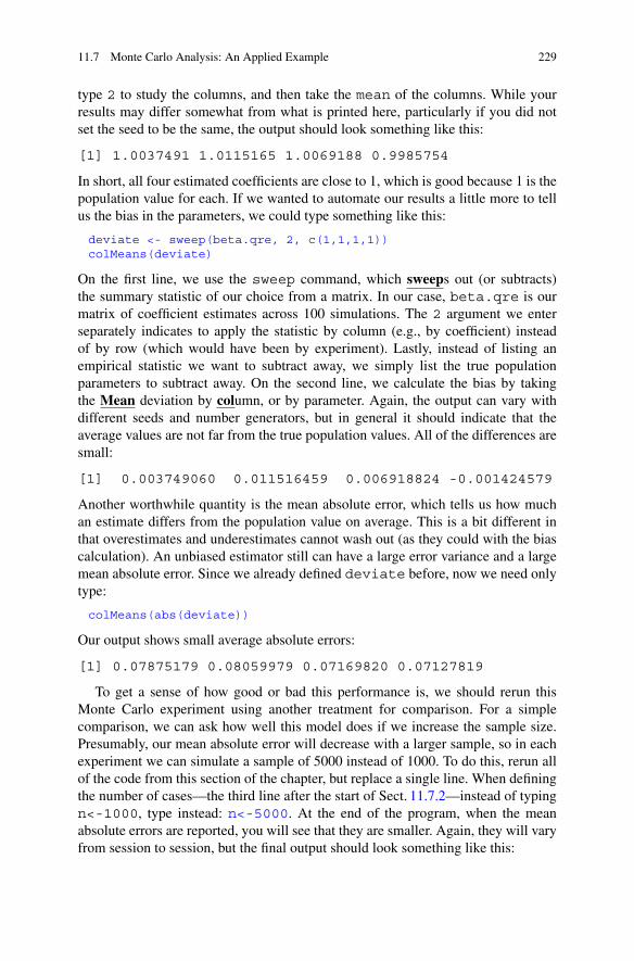
11.7 Monte Carlo Analysis: An Applied Example 229
type 2 to study the columns, and then take the mean of the columns. While yourresults may differ somewhat from what is printed here, particularly if you did notset the seed to be the same, the output should look something like this:
[1] 1.0037491 1.0115165 1.0069188 0.9985754
In short, all four estimated coefficients are close to 1, which is good because 1 is thepopulation value for each. If we wanted to automate our results a little more to tellus the bias in the parameters, we could type something like this:
deviate <- sweep(beta.qre, 2, c(1,1,1,1))colMeans(deviate)
On the first line, we use the sweep command, which sweeps out (or subtracts)the summary statistic of our choice from a matrix. In our case, beta.qre is ourmatrix of coefficient estimates across 100 simulations. The 2 argument we enterseparately indicates to apply the statistic by column (e.g., by coefficient) insteadof by row (which would have been by experiment). Lastly, instead of listing anempirical statistic we want to subtract away, we simply list the true populationparameters to subtract away. On the second line, we calculate the bias by takingthe Mean deviation by column, or by parameter. Again, the output can vary withdifferent seeds and number generators, but in general it should indicate that theaverage values are not far from the true population values. All of the differences aresmall:
[1] 0.003749060 0.011516459 0.006918824 -0.001424579
Another worthwhile quantity is the mean absolute error, which tells us how muchan estimate differs from the population value on average. This is a bit different inthat overestimates and underestimates cannot wash out (as they could with the biascalculation). An unbiased estimator still can have a large error variance and a largemean absolute error. Since we already defined deviate before, now we need onlytype:
colMeans(abs(deviate))
Our output shows small average absolute errors:
[1] 0.07875179 0.08059979 0.07169820 0.07127819
To get a sense of how good or bad this performance is, we should rerun thisMonte Carlo experiment using another treatment for comparison. For a simplecomparison, we can ask how well this model does if we increase the sample size.Presumably, our mean absolute error will decrease with a larger sample, so in eachexperiment we can simulate a sample of 5000 instead of 1000. To do this, rerun allof the code from this section of the chapter, but replace a single line. When definingthe number of cases—the third line after the start of Sect. 11.7.2—instead of typingn<-1000, type instead: n<-5000. At the end of the program, when the meanabsolute errors are reported, you will see that they are smaller. Again, they will varyfrom session to session, but the final output should look something like this:
230 11 Additional Programming Tools
[1] 0.03306102 0.02934981 0.03535597 0.02974488
As you can see, the errors are smaller than they were with 1000 observations. Oursample size is considerably bigger, so we would hope that this would be the case.This gives us a nice comparison.
With the completion of this chapter, you now should have the toolkit necessaryto program in R whenever your research has unique needs that cannot be addressedby standard commands, or even user-contributed packages. With the completion ofthis book, you should have a sense of the broad scope of what R can do for politicalanalysts, from data management, to basic models, to advanced programming. A truestrength of R is the flexibility it offers users to address whatever complexities andoriginal problems they may face. As you proceed to use R in your own research,be sure to continue to consult with online resources to discover new and promisingcapabilities as they emerge.
11.8 Practice Problems
1. Probability distributions: Calculate the probability for each of the followingevents:
a. A standard normally distributed variable is larger than 3.b. A normally distributed variable with mean 35 and standard deviation 6 is
larger than 42.c. X < 0:9 when x has the standard uniform distribution.
2. Loops: Let h.x; n/ D 1 C x C x2 C � � � C xn D PniD0 xi. Write an R program to
calculate h.0:9; 25/ using a for loop.3. Functions: In the previous question, you wrote a program to calculate h.x; n/ DPn
iD0 xi for x D 0:9 and n D 25. Turn this program into a more general functionthat takes two arguments, x and n, and returns h.x; n/. Using the function,determine the values of h.0:8; 30/, h.0:7; 50/, and h.0:95; 20/.
4. Maximum likelihood estimation. Consider an applied example of Signorino’s(1999) strategic multinomial probit method. Download a subset of nineteenthcentury militarized interstate disputes, the Stata-formatted file war1800.dta,from the Dataverse (see page vii) or this chapter’s online content (see page 205).These data draw from sources such as EUGene (Bueno de Mesquita and Lalman1992) and the Correlates of War Project (Jones et al. 1996). Program a likelihoodfunction for a model like the one shown in Fig. 11.5 and estimate the modelfor these real data. The three outcomes are: war (coded 1 if the countries wentto war), sq (coded 1 if the status quo held), and capit (coded 1 if the targetcountry capitulated). Assume that U1.SQ/ is driven by peaceyrs (number ofyears since the dyad was last in conflict) and s_wt_re1 (S score for politicalsimilarity of states, weighted for aggressor’s region). U1.W/ is a function ofbalanc (the aggressor’s military capacity relative to the combined capacity of

11.8 Practice Problems 231
the dyad). U2.W/ is a function of a constant and balanc. U1.C/ is a constant,and U2.C/ is zero.
a. Report your estimates and the corresponding standard errors.b. Which coefficients are statistically distinguishable from zero?c. Bonus: Draw the predicted probability of war if balanc is manipulated from
its minimum of 0 to its maximum of 1, while peaceyrs and s_wt_re1 are heldat their theoretical minima of 0 and �1, respectively.
• Just for fun: If you draw the same graph of predicted probabilities, butallow balanc to go all the way up to 5, you can really illustrate the kindof non-monotonic relationship that this model allows. Remember, though,that you do not want to interpret results outside of the range of your data.This is just a fun illustration for extra practice.
5. Monte Carlo analysis and optimization: Replicate the experiment on Signorino’s(1999) strategic multinomial probit from Sect. 11.7. Is there much differencebetween your average estimated values and the population values? Do you getsimilar mean absolute errors to those reported in that section? How do yourresults compare when you try the following treatments?
a. Suppose you decrease the standard deviation of x1, x2, x3, and x4 to 0.5 (asopposed to the original treatment which assumed a standard deviation of 1).Do your estimates improve or get worse? What happens if you cut the standarddeviation of these four predictors even further, to 0.25? What general patterndo you see, and why do you see it? (Remember: Everything else about thesetreatments, such as the sample size and number of experiments, needs to bethe same as the original control experiment. Otherwise all else is not beingheld equal.)
b. Bonus: What happens if you have an omitted variable in the model? Changeyour log-likelihood function to exclude x4 from your estimation procedure,but continue to include x4 when you simulate the data in the for loop. Sinceyou only estimate the coefficients for x1, x2, and x3, how do your estimatesin this treatment compare to the original treatment in terms of bias and meanabsolute error?

References
Alvarez RM, Levin I, Pomares J, Leiras M (2013) Voting made safe and easy: the impact ofe-voting on citizen perceptions. Polit Sci Res Methods 1(1):117–137
Bates D, Maechler M, Bolker B, Walker S (2014) lme4: linear mixed-effects models using Eigenand S4. R package version 1.1-7. http://www.CRAN.R-project.org/package=lme4
Becker RA, Cleveland WS, Shyu M-J (1996) The visual design and control of Trellis display.J Comput Graph Stat 5(2):123–155
Beniger JR, Robyn DL (1978) Quantitative graphics in statistics: a brief history. Am Stat32(1):1–11
Berkman M, Plutzer E (2010) Evolution, creationism, and the battle to control America’sclassrooms. Cambridge University Press, New York
Black D (1948) On the rationale of group decision-making. J Polit Econ 56(1):23–34Black D (1958) The theory of committees and elections. Cambridge University Press, LondonBox GEP, Tiao GC (1975) Intervention analysis with applications to economic and environmental
problems. J Am Stat Assoc 70:70–79Box GEP, Jenkins GM, Reinsel GC (2008) Time series analysis: forecasting and control, 4th edn.
Wiley, Hoboken, NJBox-Steffensmeier JM, Freeman JR, Hitt MP, Pevehouse JCW (2014) Time series analysis for the
social sciences. Cambridge University Press, New YorkBrambor T, Clark WR, Golder M (2006) Understanding interaction models: improving empirical
analyses. Polit Anal 14(1):63–82Brandt PT, Freeman JR (2006) Advances in Bayesian time series modeling and the study of
politics: theory testing, forecasting, and policy analysis. Polit Anal 14(1):1–36Brandt PT, Williams JT (2001) A linear Poisson autoregressive model: the Poisson AR(p) model.
Polit Anal 9(2):164–184Brandt PT, Williams JT (2007) Multiple time series models. Sage, Thousand Oaks, CABueno de Mesquita B, Lalman D (1992) War and reason. Yale University Press, New HavenCarlin BP, Louis TA (2009) Bayesian methods for data analysis. Chapman & Hall/CRC, Boca
Raton, FLChang W (2013) R graphics cookbook. O’Reilly, Sebastopol, CACleveland WS (1993) Visualizing data. Hobart Press, Sebastopol, CACowpertwait PSP, Metcalfe AV (2009) Introductory time series with R. Springer, New YorkCryer JD, Chan K-S (2008) Time series analysis with applications in R, 2nd edn. Springer,
New YorkDowns A (1957) An economic theory of democracy. Harper and Row, New YorkEliason SR (1993) Maximum likelihood estimation: logic and practice. Sage, Thousand Oaks, CA
© Springer International Publishing Switzerland 2015J.E. Monogan III, Political Analysis Using R, Use R!,DOI 10.1007/978-3-319-23446-5
233
234 References
Enders W (2009) Applied econometric time series, 3rd edn. Wiley, New YorkFitzmaurice GM, Laird NM, Ware JH (2004) Applied longitudinal analysis. Wiley-Interscience,
Hoboken, NJFogarty BJ, Monogan JE III (2014) Modeling time-series count data: the unique challenges facing
political communication studies. Soc Sci Res 45:73–88Gelman A, Hill J (2007) Data analysis using regression and multilevel/hierarchical models.
Cambridge University Press, New YorkGelman A, Carlin JB, Stern HS, Rubin DB (2004) Bayesian data analysis, 2nd edn. Chapman &
Hall/CRC, Boca Raton, FLGibney M, Cornett L, Wood R, Haschke P (2013) Political terror scale, 1976–2012. Retrieved
December 27, 2013 from the political terror scale web site: http://www.politicalterrorscale.orgGill J (2001) Generalized linear models: a unified approach. Sage, Thousand Oaks, CAGill J (2008) Bayesian methods: a social and behavioral sciences approach, 2nd edn. Chapman &
Hall/CRC, Boca Raton, FLGranger CWJ (1969) Investigating causal relations by econometric models and cross spectral
methods. Econometrica 37:424–438Granger CWJ, Newbold P (1974) Spurious regressions in econometrics. J Econ 26:1045–1066Gujarati DN, Porter DC (2009) Basic econometrics, 5th edn. McGraw-Hill/Irwin, New YorkHalley E (1686) An historical account of the trade winds, and monsoons, observable in the seas
between and near the tropicks, with an attempt to assign the phisical cause of the said winds.Philos Trans 16(183):153–168
Hamilton JD (1994) Time series analysis. Princeton University Press, Princeton, NJHanmer MJ, Kalkan KO (2013) Behind the curve: clarifying the best approach to calculating
predicted probabilities and marginal effects from limited dependent variable models. Am J PolitSci 57(1):263–277
Honaker J, King G, Blackwell M (2011) Amelia II: a program for missing data. J Stat Softw45(7):1–47
Hotelling H (1929) Stability in competition. Econ J 39(153):41–57Huber PJ (1967) The behavior of maximum likelihood estimates under nonstandard conditions.
In: LeCam LM, Neyman J (eds) Proceedings of the 5th Berkeley symposium on mathematicalstatistics and probability, volume 1: statistics University of California Press, Berkeley, CA
Iacus SM, King G, Porro G (2009) cem: software for coarsened exact matching. J Stat Softw30(9):1–27
Iacus SM, King G, Porro G (2011) Multivariate matching methods that are monotonic imbalancebounding. J Am Stat Assoc 106(493):345–361
Iacus SM, King G, Porro G (2012) Causal inference without balance checking: coarsened exactmatching. Polit Anal 20(1):1–24
Imai K, van Dyk DA (2004) Causal inference with general treatment regimes: generalizing thepropensity score. J Am Stat Assoc 99(467):854–866
Jones DM, Bremer SA, Singer JD (1996) Militarized interstate disputes, 1816–1992: rationale,coding rules, and empirical patterns. Confl Manag Peace Sci 15(2):163–213
Kastellec JP, Leoni EL (2007) Using graphs instead of tables in political science. Perspect Polit5(4):755–771
Keele L, Kelly NJ (2006) Dynamic models for dynamic theories: the ins and outs of laggeddependent variables. Polit Anal 14(2):186–205
King G (1989) Unifying political methodology. Cambridge University Press, New YorkKing G, Honaker J, Joseph A, Scheve K (2001) Analyzing incomplete political science data: an
alternative algorithm for multiple imputation. Am Polit Sci Rev 95(1):49–69Koyck LM (1954) Distributed lags and investment analysis. North-Holland, AmsterdamLaird NM, Fitzmaurice GM (2013) Longitudinal data modeling. In: Scott MA, Simonoff JS, Marx
BD (eds) The Sage handbook of multilevel modeling. Sage, Thousand Oaks, CALaLonde RJ (1986) Evaluating the econometric evaluations of training programs with experimental
data. Am Econ Rev 76(4):604–620Little RJA, Rubin DB (1987) Statistical analysis with missing data, 2nd edn. Wiley, New York
References 235
Long JS (1997) Regression models for categorical and limited dependent variables. Sage,Thousand Oaks, CA
Lowery D, Gray V, Monogan JE III (2008) The construction of interest communities: distinguish-ing bottom-up and top-down models. J Polit 70(4):1160–1176
Lütkepohl H (2005) New introduction to multiple time series analysis. Springer, New YorkMartin AD, Quinn KM, Park JH (2011) MCMCpack: Markov chain Monte Carlo in R. J Stat Softw
42(9):1–21Mátyás L, Sevestre P (eds) (2008) The econometrics of panel data: fundamentals and recent
developments in theory and practice, 3rd edn. Springer, New YorkMcCarty NM, Poole KT, Rosenthal H (1997) Income redistribution and the realignment of
American politics. American enterprise institute studies on understanding economic inequality.AEI Press, Washington, DC
Monogan JE III (2011) Panel data analysis. In: Badie B, Berg-Schlosser D, Morlino L (eds)International encyclopedia of political science. Sage, Thousand Oaks, CA
Monogan JE III (2013a) A case for registering studies of political outcomes: an application in the2010 House elections. Polit Anal 21(1):21–37
Monogan JE III (2013b) Strategic party placement with a dynamic electorate. J Theor Polit25(2):284–298
Nocedal J, Wright SJ (1999) Numerical optimization. Springer, New YorkOwsiak AP (2013) Democratization and international border agreements. J Polit 75(3):717–729Peake JS, Eshbaugh-Soha M (2008) The agenda-setting impact of major presidential TV addresses.
Polit Commun 25:113–137Petris G, Petrone S, Campagnoli P (2009) Dynamic linear models with R. Springer, New YorkPfaff B (2008) Analysis of Integrated and cointegrated time series with R, 2nd edn. Springer,
New YorkPlayfair W (1786/2005) In: Wainer H, Spence I (eds) Commercial and political atlas and statistical
breviary. Cambridge University Press, New YorkPoe SC, Tate CN (1994) Repression of human rights to personal integrity in the 1980s: a global
analysis. Am Polit Sci Rev 88(4):853–872Poe SC, Tate CN, Keith LC (1999) Repression of the human right to personal integrity revisited: a
global cross-national study covering the years 1976–1993. Int Stud Q 43(2):291–313Poole KT, Rosenthal H (1997) Congress: a political-economic history of roll call voting. Oxford
University Press, New YorkPoole KT, Lewis J, Lo J, Carroll R (2011) Scaling roll call votes with wnominate in R. J Stat
Softw 42(14):1–21Rabinowitz G, Macdonald SE (1989) A directional theory of issue voting. Am Polit Sci Rev
83:93–121Robert CP (2001) The Bayesian choice: from decision-theoretic foundations to computational
implementation, 2nd edn. Springer, New YorkRubin DB (1987) Multiple imputation for nonresponse in surveys. Wiley, New YorkRubin DB (2006) Matched sampling for causal effects. Cambridge University Press, New YorkScott MA, Simonoff JS, Marx BD (eds) (2013) The Sage handbook of multilevel modeling. Sage,
Thousand Oaks, CASekhon JS, Grieve RD (2012) A matching method for improving covariate balance in cost-
effectiveness analyses. Health Econ 21(6):695–714Shumway RH, Stoffer DS (2006) Time series analysis and its applications with R examples, 2nd
edn. Springer, New YorkSignorino CS (1999) Strategic interaction and the statistical analysis of international conflict. Am
Polit Sci Rev 93:279–297Signorino CS (2002) Strategy and selection in international relations. Int Interact 28:93–115Signorino CS, Yilmaz K (2003) Strategic misspecification in regression models. Am J Polit Sci
47:551–566Sims CA, Zha T (1999) Error bands for impulse responses. Econometrica 67(5):1113–1155

236 References
Singh SP (2014a) Linear and quadratic utility loss functions in voting behavior research. J TheorPolit 26(1):35–58
Singh SP (2014b) Not all election winners are equal: satisfaction with democracy and the natureof the vote. Eur J Polit Res 53(2):308–327
Singh SP (2015) Compulsory voting and the turnout decision calculus. Polit Stud 63(3):548–568Tufte ER (2001) The visual display of quantitative information, 2nd edn. Graphics Press, Cheshire,
CTTukey JW (1977) Exploratory data analysis. Addison-Wesley, Reading, PAWakiyama T, Zusman E, Monogan JE III (2014) Can a low-carbon-energy transition be sustained
in post-Fukushima Japan? Assessing the varying impacts of exogenous shocks. Energy Policy73:654–666
Wei WWS (2006) Time series analysis: univariate and multivariate methods, 2nd edn. Pearson,New York
White H (1980) A heteroskedasticity-consistent covariance matrix estimator and a direct test forheteroskedasticity. Econometrica 48(4):817–838
Yau N (2011) Visualize this: the FlowingData guide to design, visualization, and statistics. Wiley,Indianapolis

Index
Symbols113th US Senate roll call data, 15, 155
Aabline, 36, 42, 44, 58, 211, 217abs, 227, 229acf, 159, 162adf.test, 159American National Election Study, 31, 124anova, 87apply, 38, 194, 212, 228arima, 161, 163arimax, 164, 184arithmetic commands, 6, 24, 88, 166, 184, 209,
213, 214, 219, 226, 227transcendental functions, 6, 106, 114, 118,
196, 226with matrices and vectors, 196
arrows, 46as.data.frame, 19, 106–108, 122, 192,
193, 202as.factor, 25, 112as.matrix, 149, 163, 183, 192, 226as.numeric, 21, 25, 102, 184assignment operator (<-), 8, 14att, 145, 147attach, 18Augmented Dickey-Fuller test, 159axis, 37, 44–46, 166
Bbarplot, 38, 39, 58Bayesian methods, 134
linear regression, 134logistic regression, 138nonconvergence diagnostics, 137, 139
bgtest, 169Boolean statements, 20, 24, 81, 102, 129, 134,
166, 184, 205, 213, 220, 227bootstrapping, 180, 194box, 36, 37, 58, 166Box.test, 163boxplot, 36, 37bptest, 89Breusch-Godfrey test, 97, 170Breusch-Pagan test, 89
Cc, 16, 188, 201cat, 8causality, 178, 180cbind, 106–108, 122, 190, 193, 201, 202, 227cem, 143, 147cemspace, 145chol, 202class, 220cochrane.orcutt, 171coef, 184coeftest, 89colMeans, 229colnames, 16, 106–108, 122, 193, 220command prompt, 3comments (#), 5, 216, 220Comparative Study of Electoral Systems, 100,
110, 123, 131, 138confint, 84Cook’s distances, 95
© Springer International Publishing Switzerland 2015J.E. Monogan III, Political Analysis Using R, Use R!,DOI 10.1007/978-3-319-23446-5
237

238 Index
cor, 75correlation coefficient (r), 74, 160cross-tabulations, 71CrossTable, 71
Ddata
merging, 26missing, 14, 22panel data formatting, 29reading in, 14recoding, 21, 24reshaping, 29subsetting, 23viewing, 19writing out, 18
data frame, 17, 192democratization and international border
settlements data, 96densityplot, 48densplot, 138descriptive statistics
central tendency, 54dispersion measures, 60frequency tables, 57inter-quartile range, 56mean, 54, 194median, 56median absolute deviation, 60mode, 58percentiles, 61quantiles, 61standard deviation, 60variance, 60, 194
det, 197detach, 18dev.off, 49diag, 192, 217, 227dim, 28, 194dotplot, 48drug policy coverage data, 50, 62, 125Durbin-Watson test, 88, 169dwtest, 88, 169
Eenergy policy coverage data, 34, 117, 158, 186error message, 4, 195
Ffile.choose, 17fitted, 184
fix, 19for, 210, 213, 214, 220, 227foreign, 138function, 207, 209, 215, 219, 220, 226
default values, 221
Ggeneralized linear model, 99
for binary outcomes, 100for count outcomes, 116for ordinal outcomes, 110link function, 99, 105, 112, 114, 115, 117,
118getwd, 7, 19geweke.diag, 137, 139glm, 99
family argument, 99for logit model, 101, 103for Poisson model, 117for probit model, 104
glmer, 132graphs
bar graph, 38, 39, 59box-and-whisker plot, 36, 37density plot, 48, 55, 137, 138dot plot, 47histogram, 35, 36, 48, 91jittering, 86line plot, 43, 108, 110, 123, 167, 168, 208,
210, 218quantile-quantile plot, 91saving, 49scatterplot, 41, 47, 76, 86, 87, 153spike plot, 45, 212univariate, 35
grep, 184
Hhat values, 95head, 19, 26, 28, 29, 149health lobbying state data, 34help files, 10hist, 35, 91histogram, 48
II, 88if, 212, 213
if...else, 213, 214imbalance, 141, 144, 147influenceIndexPlot, 94

Index 239
input code, 4installing R , 2invisible, 208, 220IQR, 56irf, 180, 181is, 22is.data.frame, 22is.matrix, 22is.na, 22, 81, 129, 134Israeli-Palestinian conflict weekly actions data,
158, 176
JJapanese electricity consumption data, 185Jarque-Bera test, 92jitter, 87jpeg, 50
Kkronecker, 197kurtosis, 91
Llag, 172, 174LATEX, 83legend, 46, 107, 122, 152length, 149, 188, 194, 220levels, 25lines, 43, 46, 107, 109, 122, 166, 184list, 17, 188, 220list, 146, 220Ljung-Box Q-test, 162lm, 42, 79, 81, 168, 202, 218
dyn$lm, 172, 174coefficients, 174fitted.values, 43, 85product terms, 81residuals, 85, 90, 91
lmer, 129logistic regression, 101, 102
AIC, 102, 104Bayesian, 138deviance, 102odds ratio, 106percent correctly predicted, 102predicted probabilities, 106z-ratio, 102
ls, 9, 129, 134, 141, 148, 226
Mmad, 60
match, 184matching
average treatment effect on the treated, 145balance, 141Coarsened Exact Matching, 140
matrix, 17, 187, 192addition, 195commands for, 194creating, 189determinant, 197diagonal, 192formula for OLS, 198indices, 149, 166, 183, 184, 191, 193, 220,
226inverse, 197, 199, 201, 217, 227Kronecker product, 197matrix algebra, 195matrix formula for OLS, 201multiplication (%*%), 166, 184, 196, 197,
201, 226print, 190–192
matrix, 149, 189, 191, 192, 194, 211, 220,227
maximum likelihood estimation, 215likelihood function, 215, 226log-likelihood function, 215, 217, 226optimizing, 216, 227programming, 215standard errors, 217
MCMClogit, 138, 139MCMCmetrop1R, 134MCMCregress, 134mean, 54, 194, 211, 228measurement models, 147median, 56merge, 28mtext, 46, 107multilevel models, 128
linear, 128logistic, 131
NNA, 14, 22, 81, 129, 134, 191, 211, 220, 227na.omit, 22, 81names, 220
data, 19linear regression, 85vector, 39
naming objects, 5National Supported Work Demonstration, 53,
63, 141National Survey of High School Biology
Teachers, 79, 128, 134

240 Index
negative binomial regression, 119AIC, 120overdispersion parameter, 120predicted counts, 121
Oobjects, 9optim, 202, 215, 216, 227options
digits, 6, 57scipen, 141
order, 43order statistics, 54ordered, 112ordered logit model, 112
cutpoints, 113fit statistics, 113interaction terms, 112odds ratio, 114one-tailed p-value, 114z-ratio, 113
ordered probit model, 115output printout, 4
Ppacf, 159, 162packages, 9, 127
Amelia, 22, 155base, 33, 35, 40, 45boot, 194car, 24, 93, 94cem, 54, 64, 141coda, 137dlm, 183dyn, 172foreign, 17, 38, 80, 100, 111, 129, 134,
176ggplot2, 34gmodels, 71install.packages command, 10, 24,
47, 71, 88, 89, 92, 129, 134, 141,148, 164, 171, 172, 176
lattice, 33, 47, 50library command, 10, 47, 71, 88, 89, 92,
100, 111, 112, 129, 132, 134, 141,148, 164, 171, 172, 176
lme4, 129, 132lmtest, 88, 169MASS, 112, 119, 206maxLik, 215MCMCpack, 10, 134, 137, 138mice, 22
mvtnorm, 206orcutt, 171plm, 97sandwich, 89TSA, 160, 164, 178, 183tseries, 92, 159vars, 176wnominate, 147, 148xtable, 83
panel data, 96par, 40, 46pbgtest, 97pdf, 50plm, 97, 183plot, 33, 35, 40, 45, 75, 85, 87, 107, 109, 122,
150, 152, 166, 184, 208, 209, 211,217
png, 50pnorm, 109, 114points, 46, 152, 166, 184Poisson regression, 117
AIC, 118count ratio, 118predicted counts, 121z-ratio, 118
Political Terror Scale data, 13polr, 112, 115polygon, 46postscript, 49predict, 121
glm, 102, 106–108, 122nb.glm, 122
print, 8optim output, 216
probability distributions, 9, 206cumulative distribution function, 109, 114,
206, 209, 219, 226probability density function, 207probability mass function, 207quantile function, 207random draws from, 192, 194, 206, 211,
227probit regression, 104
predicted probabilities, 108confidence intervals, 109, 110
programming, 205branching, 212–214function definition, 207, 219
log-likelihood function, 215, 226function output, 207, 217, 220, 226loops, 210, 213, 214, 220, 227Monte Carlo analysis, 223object-oriented programming, 217, 220
class, 218

Index 241
objects, 218S3 object family, 218, 222S4 object family, 218, 220, 222, 223
optimization, 215set seed for random number generator, 211,
227
Qq, 9qqnorm, 91quantile, 61
RRamsey’s RESET test, 87rbind, 190read.csv, 15, 26, 35, 117, 158, 183read.delim, 15read.dta, 17, 38, 80, 100, 111, 129, 132,
134, 138, 176read.fwf, 15read.spss, 17read.table, 14recode, 25regression
Bayesian linear, 134Bayesian logistic, 138confidence interval, 84F-ratio for model comparison, 87F-ratio for model fit, 83Feasible Generalized Least Squares, 170functional form diagnostics, 85Gauss-Markov Theorem, 85heteroscedasticity diagnostics, 89Huber-White standard errors, 89interaction terms, 82, 112linear, 42, 79, 83, 198, 202logistic, 101matrix formula for OLS, 198multicollinearity, 93multilevel, 128negative binomial model, 119non-normal residual diagnostics, 90ordered logit, 112ordered probit, 115outliers, leverage, and influence points, 94Poisson, 117probit, 104R2, 83t-ratio, 83, 90time series, 167two-tailed p-value, 83, 90Weighted Least Squares, 90
relevel, 25rep, 37, 189, 201, 220, 227reshape, 29, 30return, 207, 219, 226rm, 9, 19, 129, 134, 141, 148, 226roll call analysis, 147rollcall, 149rownames, 193, 220
SSalta e-voting experiment, 76, 154sample, 194, 206, 213, 214script files, 7sd, 60seq, 106, 108, 122, 189, 208, 209,
217set.seed, 194, 211, 227setClass, 220setwd, 7, 19, 152sink, 8skew, 91solve, 197, 201, 217, 227sqrt, 217, 227strategic deterrence game, 223strategic multinomial probit, 223stripplot, 48Studentized residuals, 95subset, 23, 27, 38, 81, 129, 134, 152, 176,
183sum, 102, 194, 214summary
Bayesian linear regression, 135Bayesian logistic regression, 139data, 20, 56, 81linear model, 172linear regression, 42, 82, 168, 174logistic regression, 101, 103multilevel logit model, 132negative binomial regression, 119ordered logit model, 113Poisson regression, 117probit regression, 105W-NOMINATE, 150
sweep, 229
Tt, 196, 201t-ratio
for a regression coefficient, 83, 90for a single mean, 64paired, 69two sample, 66

242 Index
t.testfor a single mean, 65paired, 69two sample, 67
table, 22, 57, 102text, 40, 46tiff, 50time series, 157
AIC, 165, 177ARIMA model, 158, 161, 163, 164autocorrelation function, 159, 160, 162,
178, 179Box-Jenkins approach, 158Cochrane-Orcutt estimator, 171dynamic model, 163, 172–174econometric approaches, 167Feasible Generalized Least Squares, 170further resources, 181Granger causality test, 176, 178, 180impulse response analysis, 180–182integrated (unit root), 159Koyck model, 172, 173lag, 159, 172, 174, 176orthogonalization of residuals, 180single and multiple equation models, 157static model, 163, 168, 170stationary and nonstationary, 158transfer function, 164trending, 159unrestricted distributed lag, 174variable ordering, 180vector autoregression, 175, 177, 179
trellis.device, 50ts, 167, 172, 183, 184tsdiag, 162
UU.N. roll call vote data, 148U.S. congressional election 2010 data
Arizona, 203Tennessee, 188
U.S. congressional election 2010 dataArizona, 202Tennessee, 187
U.S. monetary and economic data, 186
VVAR, 177var, 60, 194variable or attribute referencing ($), 18, 35,
143, 152, 162, 166, 177, 183, 217,222, 223
variance inflation factor, 93VARselect, 177vcovHC, 89vector, 17
addition, 195character, 25commands for, 194creating, 188factor, 25indices, 184, 193inner product (%*%), 196numeric, 17, 21, 146omitting a term, 106, 118outer product (%o%), 196sequential count (:), 166, 183, 189vector algebra, 195
View, 19vif, 93
Wwhich.max, 58, 220while, 210wnominate, 149working directory, 7, 19write.csv, 18, 152write.dta, 18write.table, 18
Xxtable, 83, 102xyplot, 47
Zz-ratio
for logit model, 102for ordered logit model, 113for Poisson model, 118