J. Vis. Commun. Image R. 22 (2011) 653–663

Contents lists available at SciVerse ScienceDirect

J. Vis. Commun. Image R.

journal homepage: www.elsevier .com/ locate/ jvc i

High-quality non-blind image deconvolution with adaptive regularization

Jong-Ho Lee ⇑, Yo-Sung HoGwangju Institute of Science and Technology (GIST), 1 Oryong-dong, Buk-gu, Gwangju 500-712, Republic of Korea

a r t i c l e i n f o a b s t r a c t

Article history:Received 14 December 2010Accepted 15 July 2011Available online 23 July 2011

Keywords:Image deblurringNon-blind image deconvolutionRinging artifactsNoise amplificationLocal characteristicsAdaptive regularizationFast deconvolutionBoundary artifacts reduction

1047-3203/$ - see front matter � 2011 Elsevier Inc. Adoi:10.1016/j.jvcir.2011.07.010

⇑ Corresponding author.E-mail addresses: purmod@imrc.kist.re.kr (J.-H. Lee

Non-blind image deconvolution is a process that obtains a sharp latent image from a blurred image whena point spread function (PSF) is known. However, ringing and noise amplification are inevitable artifactsin image deconvolution since perfect PSF estimation is impossible. The conventional regularization toreduce these artifacts cannot preserve image details in the deconvolved image when PSF estimation erroris large, so strong regularization is needed. We propose a non-blind image deconvolution method whichpreserves image details, while suppressing ringing and noise artifacts by controlling regularizationstrength according to local characteristics of the image. In addition, the proposed method is performedfast with fast Fourier transforms so that it can be a practical solution to image deblurring problems. Fromexperimental results, we have verified that the proposed method restored the sharp latent image withsignificantly reduced artifacts and it was performed fast compared to other non-blind image deconvolu-tion methods.

� 2011 Elsevier Inc. All rights reserved.

1. Introduction

One of the most common and unpleasant defects in photographyis motion blur caused by camera shake. Especially, if a picture is ta-ken in the dim light conditions, it takes long time to get enough lightand the camera shake by hands results in a degraded image. If a mo-tion blur is shift-invariant, recovering a true latent image from thedegraded image reduces to image deconvolution. The blurring pro-cess is commonly modeled as a convolution of the true latent imageand a point spread function (PSF) with additive noise:

B ¼ K � I þ N; ð1Þ

where B is the degraded image, I is the true latent image, K is thePSF, and N is additive noise. Image deconvolution is a process to re-store I from B.

If both the PSF and the latent image are unknown, the problemis called blind deconvolution. In blind deconvolution, the problemis challenging since both PSF and the latent image should be esti-mated from the blurred image. Thus, to facilitate the problem,early approaches assume simple parametric models for the PSFsuch as linear motion blur or out-of focus blur [1,2]. Additionalinput was also used in some methods. Ben-Ezra and Nayarattached a low-resolution video camera to a high-resolution stillcamera to help in recording the PSF [3]. Yuan et al. used a pair ofimages, a blurred image and a noisy image which was taken withfast shutter speed, to estimate the PSF and the latent image [4].

ll rights reserved.

), hoyo@gist.ac.kr (Y.-S. Ho).

Recently, the PSF was estimated from a single image. Fergus etal. used a variational Bayesian method with natural image statis-tics to estimate the PSF [5]. Jia used an alpha matte that describestransparency changes caused by a motion blur for PSF estimation[6]. Shan et al. proposed the blind deconvolution method using amaximum a posteriori (MAP) to estimate both the PSF and the la-tent image from a single image [7]. However, it is very difficult toestimate the exact PSF from a single image. For example, the satu-rated pixels or homogeneous region on the blurred image preventthe PSF from being estimated correctly.

On the other hand, if the PSF is assumed to be known or esti-mated in other ways, the problem is reduced to estimate the latentimage alone. This is called non-blind image deconvolution. Wienerfiltering [8] and Richardson–Lucy method [9] are traditional andpopular non-blind image deconvolution methods. Although thesemethods were proposed several decades ago, they are still widelyused for image restoration because they are simple, fast, and givegood results in case of the relative small blur. However, non-blinddeconvolution is still an ill-posed problem although the PSF isknown, so it gives rise to artifacts in the deconvolved image. Themain artifacts are ringing and noise amplification. Fig. 1 showsthe deconvolution result. Ringing is the ripple-like artifact that ap-pears around strong edges in the deconvolved image as shown inFig. 1(c). The PSF is often band-limited, so its frequency responseshows zero or near-zero values at the high frequency. Therefore,the direct inverse of the PSF with the blurred image causes largesignal amplification at the high frequency components and this isrepresented as the ringing near the edges and amplified noise.Especially, PSF estimation errors accelerate the ringing artifacts

Fig. 1. Ringing artifacts in image deconvolution. (a) Blurred image and estimated PSF. (b) Deconvolution result. (c) Magnified patch.

654 J.-H. Lee, Y.-S. Ho / J. Vis. Commun. Image R. 22 (2011) 653–663

and give very unpleasant deconvolved results [7]. Various regular-ization techniques to reduce these artifacts are proposed. Cham-bolle and Lions proposed total variation regularization withLaplacian prior [10]. Levein et al. used a sparse prior with heavy-tailed distribution that shows quite good results with significantlyreduced artifacts [11]. Shan et al. also exploit the image prior de-fined on their own to reduce artifacts in the deconvolved image[7]. Recently, Cho et al. proposed a content-aware image priorwhich adapt prior to the image contents. This prior is more effec-tive to recover the latent image than other fixed image priors sincethe gradient profile of the image is changed according to textures[23]. All of them introduce image prior into the deconvolution, sothey solve the MAP problem instead of maximum likelihood (ML)estimation. However, all these regularization methods using theMAP are effective only when the PSF size is small and the esti-mated PSF has no error. If the PSF size is large and the estimatedPSF is incorrect, then the deconvolved image contains severe ring-ing or amplified noise. The strong regularization to reduce thesesevere artifacts destroys the image details in the deconvolved im-age, and this is inevitable problem in image deblurring since per-fect PSF estimation is impossible.

We propose a non-blind image deconvolution method withadaptive regularization that controls the regularization strengthadaptively according to the local characteristics. It reduces ringingand noise in a smooth region effectively and preserves image de-tails in a textured region simultaneously. For adaptive regulariza-tion, we make reference maps that give right edge information sothat textured region and smooth region can be distinguished well.Regularization strength is controlled adaptively referring to thesereference maps. There are other several methods exploiting pilotimages like reference maps in our algorithm to improve qualityof deconvolution. Lou et al. use the deconvolved image with Tikho-nov regularization as their pilot image for computing weights ofnon-local operator [24]. Takeda et al. also estimate the pilot imageby Wiener filtering followed by kernel regression to computeweight matrix [25]. Dabov et al. use the regularized inversion usingBM3D filter to estimate the pilot image [26]. All these pilot imagesare the estimates of the deconvolution results, so they give impor-tant information for deconvolution, and enable better deconvolu-tion results to be achieved. However, since all pilot images inthese methods are estimated using very simple method for compu-tational advantage, they suffer from ringing artifacts when the esti-mated PSF is not correct and these artifacts in pilot images havebad influence on the final results. In our algorithm, the referencemaps are elaborated using both blurred image and deconvolvedimage by adaptive regularization with hyper-Laplacian imageprior. Thus, they give well-defined edge and texture information.Furthermore, proposed image deconvolution with adaptive regu-larization is performed very fast in the frequency domain usingthe fast Fourier transforms (FFTs). The experimental results showthat the latent image with high-quality is recovered very fast from

the blurred image compared to other various non-blind imagedeconvolution methods.

The rest of this paper is organized as follows. In the next Sec-tion, we will briefly review the conventional regularization tech-niques and present its limitations on recovering the high-qualitylatent image. In Section 3, we will introduce the high-qualitynon-blind image deconvolution with adaptive regularization. InSection 4, performance of the proposed method will be verifiedand the paper will be completed with conclusions in Section 5.

2. Conventional regularization methods

The most basic form of regularization is the Tikhonov regulari-zation [12]. It is given as follows:

I� ¼ arg minI

XN

i¼1

ððI � K � BÞ2i þ gjIij2Þ; ð2Þ

where i is the pixel index, and g is the regularization weighting fac-tor that controls strength of regularization. Tikhonov regularizationreduces artifacts quite well, but since it assumes the image to besmooth and continuous, it produces smooth results and fails to re-cover the sharper edges.

More advanced regularization techniques are proposed usingthe image prior. According to Bayes’ theorem, the posteriori forthe latent image is written as:

pðIjBÞ / pðBjIÞpðIÞ; ð3Þwhere p(BjI) denotes the likelihood of the blurred image given thelatent image, and p(I) represents the image prior. The MAP solutionof I can be obtained by minimizing the following energy:

I� ¼ arg minI

EðIÞ; ð4Þ

where

EðIÞ ¼ � log pðIjBÞ ¼ � log pðBjIÞ � log pðIÞ: ð5ÞThe likelihood is based on noise, N = B � I � K, and it can be as-sumed to follow Gaussian distribution [11] or Poisson distribution[13]. If the noise model is Gaussian and the image prior is assumedthat the first derivative of image follows Laplacian distribution, Eq.(5) can be represented as:

EðIÞ ¼XN

i¼1

ððI � K � BÞ2i þ gðjðI � f1Þij þ jðI � f2ÞijÞÞ; ð6Þ

where f1 = [1 � 1], f2 = [1 � 1]T, and g is the regularization weight-ing factor. This regularization technique is called total variation,and it takes into consideration the information that the image dataset is blocky and discontinuous [10]. This method helps to obtainthe discontinuities or steep gradients in the restored image.

Recently, various studies on global images have shown that theimage gradients have heavier tails than a Gaussian or Laplaciandistribution. Roth and Black modeled image statistics with a prod-uct of potentials defined on filter outputs [14]. Weiss and Freeman

Fig. 2. Deconvolution results with conventional regularization. (a) Blurred image and estimated PSF (b) Strong regularization result. (c) Weak regularization result.

J.-H. Lee, Y.-S. Ho / J. Vis. Commun. Image R. 22 (2011) 653–663 655

used Gaussian Scale Mixture Fields of Experts (GSM FOE) model forimage prior [15]. A simpler form of the heavy-tailed distribution ofimage gradients is the hyper-Laplacian model. Hyper-Laplacianimage priors have been often used in image deblurring [11,16].The hyper-Laplacian image prior can be modeled as:

pðIÞ / e�kjOIja with 0:5 6 a 6 0:8: ð7Þ

With the Gaussian noise model and the hyper-Laplacian imageprior, Eq. (5) can be represented by

EðIÞ ¼XN

i¼1

ððI � K � BÞ2i þ gðjðI � f1Þija þ jðI � f2Þij

aÞÞ; ð8Þ

where g is the regularization weighting factor.On the other hand, Yuan et al. also proposed a regularization

technique using a bilateral filter [17]. Although this regularizationtechnique shows excellent results with preserved edges and re-duced artifacts, it takes too much time to obtain a final resultdue to repetitive intra- and inter-scaling and filtering operationin each scale.

In all above conventional regularization techniques, the regular-ization weighting factor, g is applied to all pixels with the sameintensity. Fig. 2 represents the deconvolution results with conven-tional regularization. The left one shows the deconvolution resultwith strong regularization and the right one is that of weak regu-larization. Levin’s method was used for image deconvolution, andthe regularization weighting factors of 0.1 � 10�1 and 0.1 � 10�9

were used for strong regularization and weak regularizationrespectively. Strong regularization in the image deconvolutionhelps to reduce the artifacts in the smooth region, but it blursthe edges in the textured region. Weak regularization preservesimage details well, but it does not remove artifacts effectively.Therefore, the conventional regularization has limitations if thePSF estimation error is large or image noise is too severe to be ig-nored. Large PSF estimation error and severe noise give rise to se-vere ringing and noise amplification and those severe artifactsrequire strong regularization which destroys image details.

Furthermore, Eq. (8) is not a convex function, so it is difficult toget a solution optimizing Eq. (8). Commonly used method is aniteratively reweighted least squares (IRLS) method that solves aseries of weighted least-squares problems with conjugate gradient(CG) [11]. In this method, since typically hundreds of CG iterations,each involving an expensive convolution of the current image esti-mate and the PSF, are needed, it takes too much time to process.

3. High-quality non-blind image deconvolution with adaptiveregularization

The main idea of our algorithm is to change strength of regular-ization based on the reference map which indicates the smoothed

region and textured region. In the smooth region, strong regulari-zation is performed to suppress the artifacts and in the textured re-gion, weak regularization is applied to preserve image details. Thefirst reference map is estimated from the blurred image and thefirst adaptive regularization is performed based on the first refer-ence map. Since the blurred image does not show right edge infor-mation, the first adaptive regularization does not work well. Thus,the second reference map is estimated using the first deconvolvedimage, and the second adaptive regularization is executed with thesecond reference map. All adaptive regularizations are performedin the frequency domain for fast computation. However this com-putation in the frequency domain causes boundary artifacts at thedeconvolved image boundaries and these artifacts need to be re-moved. In this Section, we will cover each step of our algorithmin detail. Reference map estimation, adaptive regularization, fastcomputation of adaptive regularization, and how to reduce theboundary artifacts will be described thoroughly. The overall algo-rithm for high-quality non-blind image deconvolution with adap-tive regularization is outlined in Algorithm 1.

Algorithm 1. High-quality non-blind image deconvolutionwith adaptive regularization

Require: Blurred image B, PSF KRequire: Expansion width T, smoothness window radius rRequire: Threshold for 1st reference image estimation Ta

Require: Threshold for 2nd reference image estimation Tb

Require: Regularization weighting factor for smooth regiong1

Require: Regularization weighting factor for textured regiong2

1: B_ex = img_exp(B,T,r) %Expand blurred image for RBA2: Y = rgb2ycbcr(B)3: Y = Y(:, :,1) %Extract luma from blurred image4: for i = 1 to 25: if (i = 1) then6: Ref1 = issmooth1(Y,Ta) %Estimate 1st reference

map7: I1 = deconv_adapregu(B_ex,K,g1,g2,Ref1) %1st

adaptive regularization8: else9: Ref2 = issmooth2(B, I1,Tb) %Estimate 2nd reference

map10: I2 = deconv_adapregu(B_ex,K,g1,g2,Ref2) %2nd

adaptive regularization11: end if12: end for13: I = I2(1:size(B,1), 1:size(B,2), :)14: output: I

656 J.-H. Lee, Y.-S. Ho / J. Vis. Commun. Image R. 22 (2011) 653–663

3.1. Reference map estimation

The reference map is for classifying the smooth region and thetextured region correctly. The estimated reference map is usedfor adaptive regularization. It is difficult to obtain right edge infor-mation from the blurred image directly, so the reference map isestimated twice.

The first reference map is estimated from the blurred image.Since the smooth region which has no edges in the blurred imageis still the smooth region in the recovered image, the smooth re-gion, X, is defined as follows:

p 2 X if EgðpÞ < Ta and

EgðpÞ ¼X

h2Wx

hþX

h2Wy

v

0@

1A,Ntotal; ð9Þ

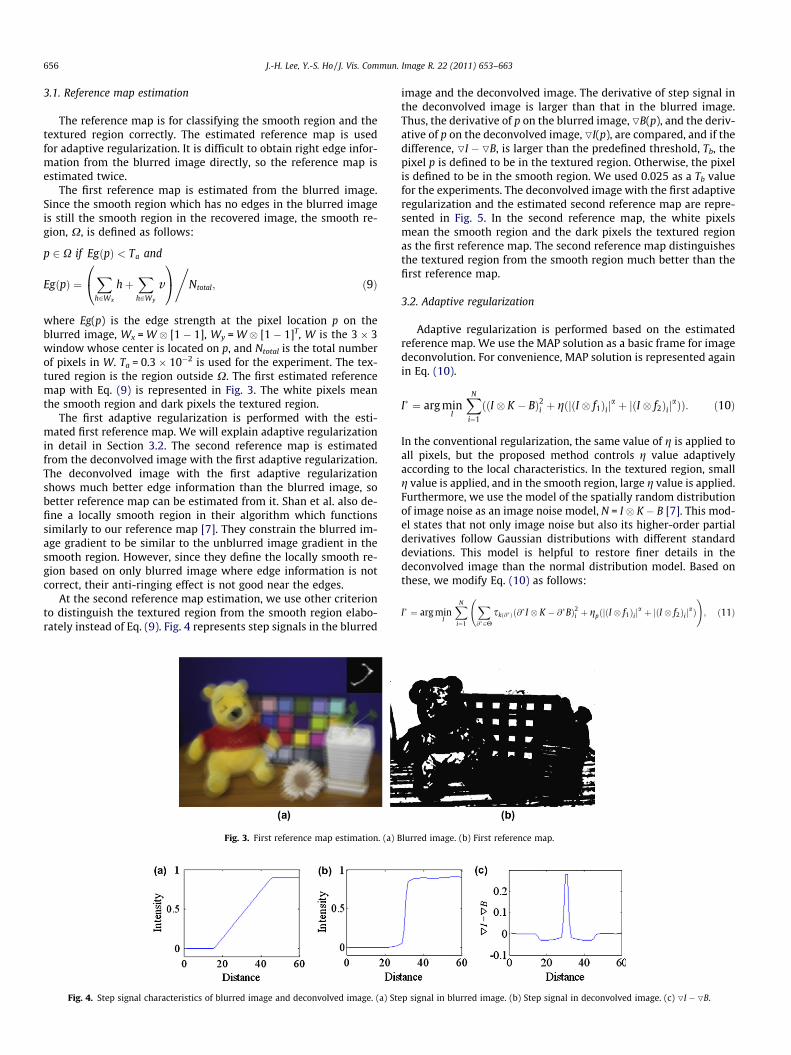
where Eg(p) is the edge strength at the pixel location p on theblurred image, Wx = W � [1 � 1], Wy = W � [1 � 1]T, W is the 3 � 3window whose center is located on p, and Ntotal is the total numberof pixels in W. Ta = 0.3 � 10�2 is used for the experiment. The tex-tured region is the region outside X. The first estimated referencemap with Eq. (9) is represented in Fig. 3. The white pixels meanthe smooth region and dark pixels the textured region.

The first adaptive regularization is performed with the esti-mated first reference map. We will explain adaptive regularizationin detail in Section 3.2. The second reference map is estimatedfrom the deconvolved image with the first adaptive regularization.The deconvolved image with the first adaptive regularizationshows much better edge information than the blurred image, sobetter reference map can be estimated from it. Shan et al. also de-fine a locally smooth region in their algorithm which functionssimilarly to our reference map [7]. They constrain the blurred im-age gradient to be similar to the unblurred image gradient in thesmooth region. However, since they define the locally smooth re-gion based on only blurred image where edge information is notcorrect, their anti-ringing effect is not good near the edges.

At the second reference map estimation, we use other criterionto distinguish the textured region from the smooth region elabo-rately instead of Eq. (9). Fig. 4 represents step signals in the blurred

Fig. 4. Step signal characteristics of blurred image and deconvolved image. (a) Ste

Fig. 3. First reference map estimation. (a) B

image and the deconvolved image. The derivative of step signal inthe deconvolved image is larger than that in the blurred image.Thus, the derivative of p on the blurred image, OB(p), and the deriv-ative of p on the deconvolved image, OI(p), are compared, and if thedifference, OI � OB, is larger than the predefined threshold, Tb, thepixel p is defined to be in the textured region. Otherwise, the pixelis defined to be in the smooth region. We used 0.025 as a Tb valuefor the experiments. The deconvolved image with the first adaptiveregularization and the estimated second reference map are repre-sented in Fig. 5. In the second reference map, the white pixelsmean the smooth region and the dark pixels the textured regionas the first reference map. The second reference map distinguishesthe textured region from the smooth region much better than thefirst reference map.

3.2. Adaptive regularization

Adaptive regularization is performed based on the estimatedreference map. We use the MAP solution as a basic frame for imagedeconvolution. For convenience, MAP solution is represented againin Eq. (10).

I� ¼ arg minI

XN

i¼1

ððI � K � BÞ2i þ gðjðI � f1Þija þ jðI � f2Þij

aÞÞ: ð10Þ

In the conventional regularization, the same value of g is applied toall pixels, but the proposed method controls g value adaptivelyaccording to the local characteristics. In the textured region, smallg value is applied, and in the smooth region, large g value is applied.Furthermore, we use the model of the spatially random distributionof image noise as an image noise model, N = I � K � B [7]. This mod-el states that not only image noise but also its higher-order partialderivatives follow Gaussian distributions with different standarddeviations. This model is helpful to restore finer details in thedeconvolved image than the normal distribution model. Based onthese, we modify Eq. (10) as follows:

I� ¼ arg minI

XN

i¼1

X@�2H

skð@�Þð@�I � K � @�BÞ2i þ gpðjðI � f1Þija þ jðI � f2Þij

aÞ !

; ð11Þ

p signal in blurred image. (b) Step signal in deconvolved image. (c) OI � OB.

lurred image. (b) First reference map.

Fig. 5. Second reference map estimation. (a) Blurred image. (b) Deconvolved image with first adaptive regularization. (c) Second reference map.

Fig. 6. Effect of adaptive regularization. (a) Blurred image. (b) Deconvolution result without adaptive regularization. (c) Deconvolution result with adaptive regularization.

J.-H. Lee, Y.-S. Ho / J. Vis. Commun. Image R. 22 (2011) 653–663 657

where @⁄ denotes the operator of any partial derivative with k(@⁄) =q representing its order. @⁄N = @⁄(I � K � B) follows a Gaussian dis-tributions with standard deviation rq = r0, where r0 denotes thestandard deviation of N. H = {@0,@x,@y,@xx,@xy,@yy} represents a setof partial derivative operators [7]. The gp is equal to 0.5 � 10�2 ifthe pixel p is located on the smooth region and 2.5 � 10�4 in thetextured region. The effect of adaptive regularization in the imagedeconvolution is represented in Fig. 6. The middle image is decon-volved result by Eq. (11) with the same gp equal to 2.5 � 10�4 forall pixels. The right image is deconvolved result with different gp

values according to the local characteristics as defined above. Theartifacts noticeable in the deconvolved result with the conventionalregularization are removed significantly in the deconvolved resultwith the adaptive regularization while preserving image details.

3.3. Fast adaptive regularization

Adaptive regularization can be performed fast in the frequencydomain with the alternating minimization. The alternating mini-mization was originally proposed by Geman et al. [18,19] and thistechnique was used for image deconvolution in various algorithms[7,20,21]. We simply modified Krishnan’s fast algorithm using hy-per-Laplacian image prior for our adaptive regularizaiton [20]. Ifwe substitute I � f1 and I � f2 with x1 and x2 respectively, Eq.(11) can be modified as follows:

I� ¼ arg minI;x

XN

i¼1

X@�2H

skð@�Þð@�I � K � @�BÞ2i þb2ððI � f1 �x1Þ2i

þ ðI � f2 �x2Þ2i Þ þkp

2ðjðx1Þij

2=3 þ jðx2Þij2=3Þ�: ð12Þ

For convenient calculation, gp is replaced with kp/2, and this doesnot affect the performance of the algorithm. (I � fj �xj)2 term isfor constraint of I � fj = xj and we use 2/3 for a. b is a weight thatis varied during the optimization. As b becomes large, the solutionof Eq. (12) is converges to that of Eq. (11). The b is varied from0.1 � 10�2 to 256 by integer powers of

ffiffiffi2p

, and for each b,

x = [x1,x2] and I are calculated alternatively. First, the initial I isset to B, and x is calculated. If fixed I is given, Eq. (12) is reducedto the problem of solving for x.

x� ¼ arg minx

kp

2jxj2=3 þ b

2ðx� mÞ2

� �; ð13Þ

where m = I � fj. x⁄ satisfying the above equation is the solution ofthe following quartic equation.

x4 � 3mx3 þ 3m2x2 � m3xþk3

p

27b3 ¼ 0: ð14Þ

The x satisfying Eq. (14) can be obtained by Ferrari’s method. Sincethe derivatives m of the image normalized to 1 are usually placedfrom �0.6 to 0.6, x values are tabulated for the specific kp, b and10,000 different values of m within the range of �0.6 and 0.6. Thus,x are obtained very fast using the table for the input images.

Given a fixed value of x from the previous iteration, Eq. (12) isquadratic in I. The optimal I is:

X@�2H

2sk @�ð ÞAT@�A@�A

Tk Ak þ b AT

f1Af1 þ AT

f2Af2

� � !i

¼X@�2H

2skð@�ÞAT@�A@�A

Tk bþ b AT

f1x1 þ AT

f2x2

� �; ð15Þ

where A@� , Ak, Af1 , and Af2 are the matrix forms of @⁄, K, f1, and f2

respectively, and i and b are vector forms of I and B such that theproduct of the matrix and vector is equal to the convolution ofthe originals. Applying 2D FFTs, we can obtain I directly as follows:

I� ¼ F�1 NumerDenom

� �; ð16Þ

where

Numer ¼X@�2H

skð@�ÞFf@�g � Ff@�g � FfKg � FfBg þ b2ðFff1g

� Ffx1g þ Fff2g � Ffx2gÞ ð17Þ

658 J.-H. Lee, Y.-S. Ho / J. Vis. Commun. Image R. 22 (2011) 653–663

and

Denom ¼X@�2H

skð@�ÞFf@�g � Ff@�g � FfKg � FfKg þ b2ðFff1g

� Fff1g þ Fff2g � Fff2gÞ: ð18Þ

Here, Ff�g and F�1{�} represent Fourier and inverse Fourier trans-form respectively, f�gmeans complex conjugate, and � meanselement-wise multiplication.

3.4. Reducing boundary artifacts

In the blurring process, the blurred pixels are generated withnot only the image inside the Field of View (FOV) of the observa-tion but also part outside the FOV. The part outside the FOV cannotbe used in the deconvolution and this missing information causesringing artifacts around the image boundary when the image isdeconvolved using the FFT. Discrete Fourier Transform (DFT) as-sumes the periodicity of the data, so the missing information willbe taken from opposite side of the image when performing FFT.However, since this data taken from the opposite side is not thesame as the original data, the boundary artifacts are occurred.

Fig. 7. Expansion of the blurred image for reducing boundary artifacts O: blurredimage A, B, C: padding blocks.

Fig. 8. Reducing boundary artifacts. (a) Blurred image and estimated PSF. (b) Deconvol

Fig. 9. Comparison of reducing boundary art

The main idea to reduce the boundary artifacts is as follows. Weexpand the original blurred image such that the intensity and gra-dient are maintained at the border between the original image andthe expanded part. The basic concept to solve the problem is sim-ilar to Liu and Jia’s algorithm [22], but our algorithm is faster andrequires lower memory achieving comparable quality since thenumber of padding blocks is smaller. Fig. 7 represents the ex-panded image for reducing boundary artifacts. O is the originalblurred image, and A, B, and C are the three padding blocks. Eachpadding block is constructed such that the periodicity of the imageis guaranteed and pixels in the padding block have smooth inten-sities not to cause ringing artifacts. We first start with the con-struction for the padding block A.

Let X(i, :) and X(:, j) denote the ith row and jth column in a imageblock X. The size of the original image is M � N and the size of thepadding block A is T � N, where T is the expansion width. The firstrow and the last row of the block A is filled first with the last rowand the first row of the original blurred image respectively.

Að1; :Þ ¼ OðM; :Þ; ð19ÞAðT; :Þ ¼ Oð1; :Þ: ð20Þ

Next, the most outer two rows of the unpadded rectangular begin tobe padded alternatively. The upper line is padded according to:

Aði; jÞ ¼Pr

k¼�rðw1kAði� 1; jþ kÞþw2kAðT � iþ 2; jþ kÞÞPrk¼�rðw1k þw2kÞ

; ð21Þ

where w1k and w2k are distances from (i, j) to (T � i + 2, j + k) andfrom (i, j) to (i � 1, j + k) respectively, and k 2 {�r, . . . , r}, and r is awindow radius that controls the smoothness in the horizontaldirection. The lower line is padded according to:

AðT � iþ 1; jÞ ¼Pr

k¼�rðw3kAði; jþ kÞþw4kAðT � iþ 2; jþ kÞÞPrk¼�rðw3k þw4kÞ

; ð22Þ

where w3k and w4k are distances from (T � i + 1, j) to (T � i + 2, j + k)and from (T � i + 1, j) to (i, j + k) respectively. This procedure isrepeated for i = 2 to T/2. The block B is constructed with the similar

ution result without RBA algorithm. (c) Deconvolution result with RBA algorithm.

ifacts algorithm. (a) Liu et al.’s. (b) Ours.

J.-H. Lee, Y.-S. Ho / J. Vis. Commun. Image R. 22 (2011) 653–663 659

manner to the block A. The only difference is the padded direction.The pixels in the block B are padded column by column.

The block C is computed after the block A and the block B areconstructed. First, the most outer pixels of the block C are paddedaccording to:

Cð:;1Þ ¼ Að:;NÞ; ð23ÞCð:; TÞ ¼ Að:;1Þ; ð24ÞCð1; :Þ ¼ BðM; :Þ; ð25ÞCðT; :Þ ¼ Bð1; :Þ: ð26Þ

Next, the inner pixels are padded:

Cði; jÞ ¼Pr

k¼�rðw1kC1k þw2kC2k þw3kC3k þw4kC4kÞPrk¼�rðw1k þw2k þw3k þw4kÞ

; ð27Þ

where C1k, C2k, C3k, and C4k are reference pixel values from theupper, bottom, left, and right directions respectively. The weightingfactors w1k, w2k, w3k, and w4k are defined according to the distancefrom the current pixel location to the reference pixel location fromeach direction. This procedure is repeated until all the other pixelsinside the block C are padded.

Fig. 10. Pooh. (a) Blurred image and estimated PSF. (b) Richardson–Lucy method. (c) T

This expanded blurred image is used for image deconvolutioninstead of the original blurred image. After image deconvolution,the result image is cropped to the original size.

Fig. 8 shows the effect of our reducing boundary artifacts (RBA)algorithm. The middle and the right images are the results of ourmethod with the same parameter setting, but the middle one usedthe general blurred image and the right one used the expandedblurred image formed according to the RBA algorithm followedby cropping to the original size after deconvolution. The boundaryartifacts in the deconvolved image without RBA algorithm are re-duced significantly with the RBA algorithm.

Fig. 9 shows the comparison of result from our RBA algorithmand Liu et al.’s. Shan et al.’s algorithm was used for image deconvo-lution [7]. Even though we use smaller number of padding blockswith smaller size than Liu et al.’s method, our result shows compa-rable performance.

4. Experimental results and analysis

We applied our algorithm to the synthesized image and thereal blurred image. The synthesized image was generated by

V regularization. (d) Levin’s. (e) Shan’s. (f) Proposed. (g) Close-up views of (a)–(f).

Fig. 11. Beer. (a) Blurred image and estimated PSF. (b) Richardson–Lucy method. (c) TV regularization. (d) Levin’s. (e) Shan’s. (f) Proposed. (g) Close-up views of (a)–(f).

660 J.-H. Lee, Y.-S. Ho / J. Vis. Commun. Image R. 22 (2011) 653–663

convolving the artificial PSF and the original sharp image. For thesynthesized image, both objective quality and subjective qualitywere checked. For the real blurred image, only subjective qualitywas measured. For testing the performance of our algorithm, wecompared the results of our algorithm to those of four othernon-blind image deconvolution methods, the standard Richard-son–Lucy (RL) method [9], Total variation (TV) regularization[10], Levin’s method [11] and Shan’s non-blind deconvolutionmethod [7]. They are popular non-blind image deconvolutionmethods due to their outstanding performances. For fare

Table 1Comparison of SNRs for the Pooh image.

Method SNR_R (dB) SNR_G (dB) SNR_B (dB) SNR_Y(dB)

RL 8.92 12.25 6.68 11.48TV 6.14 9.86 4.04 9.55Levin’s 20.76 20.05 17.95 19.75Shan’s 19.82 19.36 17.47 18.88Proposed 21.10 20.54 18.31 20.49

comparison, we tuned the regularization parameters of all algo-rithms to produce the best results.

Fig. 10 shows the comparison of the subjective quality for thesynthesized Pooh image. The PSF is estimated by Shan’s non-blindimage deconvolution algorithm [7]. The estimated PSF size is37 � 37, and the size of blurred image is 664 � 489. The RL methodpreserves edges well but produces the severe ringing and noisesince it does not exploit regularization. Besides, it is performed inthe frequency domain, so it gives rise to severe boundary artifactsin the deconvolved image. The TV regularization reduces ringing

Table 2Comparison of SNRs for the Beer image.

Method SNR_R (dB) SNR_G (dB) SNR_B (dB) SNR_Y(dB)

RL 8.65 6.41 5.82 7.76TV 7.98 5.44 3.92 6.75Levin’s 15.63 15.49 15.11 15.59Shan’s 14.74 15.20 14.95 14.96Proposed 16.06 15.79 15.38 16.09

Fig. 12. Statue. (a) Blurred image and estimated PSF. (b) Richardson–Lucy method. (c) TV regularization. (d) Levin’s. (e) Shan’s. (f) Proposed. (g) Close-up views of (a)–(f).

J.-H. Lee, Y.-S. Ho / J. Vis. Commun. Image R. 22 (2011) 653–663 661

and noise significantly, but image details are also reduced. Thereduced details are the effect of using the Laplacian image priorinstead of the hyper-Laplacian image prior. The TV regularizationalso generates the boundary artifacts due to FFT calculation. TheLevin’s algorithm and the Shan’s algorithm reduce ringing and

Table 3Comparison of complexities.

RL (secs) TV (secs) Levin’s (secs) Proposed (secs)

Pooh 91.26 75.03 329.88 66.91Beer 91.16 55.02 329.52 66.99Statue 208.86 187.98 1110.54 121.94

noise effectively without large image details loss due to advancedimage priors, but they show limitations in case of large PSF errorssince the regularization weighting factors with the same intensi-ties are applied to all pixels of the image. However, our algorithmshows the excellent result with reduced ringing and noise insmooth region, while preserving image edges well by adjustingthe regularization weighting factor according to the localcharacteristics.

Fig. 11 shows other results for the synthesized Beer image. Thecharacters in the image are clear and the artifacts such as ringingand noise in the background are reduced significantly with ouralgorithm.

For the synthesized images, the objective quality is alsomeasured. Tables 1 and 2 show the comparison of objective quality

Fig. 13. Picasso. (a) Blurred image and estimated PSF. (b) Shan’s. (c) Proposed. (d) Close-up views of (a)–(c).

Fig. 14. Red tree. (a) Blurred image and estimated PSF. (b) Richardson–Lucy method. (c) Shan’s. (d) Proposed. (e) Close-up views of (a)–(d). (For interpretation of thereferences in colour in this figure legend, the reader is referred to the web version of this article.)

662 J.-H. Lee, Y.-S. Ho / J. Vis. Commun. Image R. 22 (2011) 653–663

for Pooh and Beer images respectively. We used Eq. (28) for thecomparison metric. We calculated and compared the SNR for R,G, B channels and luminance component of the deconvolvedimages. Our algorithm shows the best performance when com-pared to other non-blind image deconvolution methods.

SNRðdBÞ ¼ 10log10kI � lðIÞk2

kI � I�k2

!; ð28Þ

where I is the original image, l(I) is the mean of I, and I⁄ is thedeconvolved image.

Next, we made an experiment with the real blurred image. Wetested the performance with the image used in [7], and the testimage was obtained from author’s website.1 The size of the blurredimage is 903 � 910, and the size of the PSF is 25 � 25. The PSF isestimated by the Fergus’ algorithm [5]. The results of our algorithmand other non-blind image deconvolution methods are

1 http://www.cse.cuhk.edu.hk/�leojia/projects/motion_deblurring/index.html.

represented in Fig. 12. The proposed method preserves fine imagedetails, while suppressing artifacts.

Furthermore, we compared the complexity of our algorithm toother non-blind image deconvolution methods. All source codesare programmed with the MATLAB, and they are tested in AMDAthlon II X2 250 processor 3.23 GHz with 2.0 GB RAM. Since theimage prior used in the proposed method is hyper-Laplacian, theenergy function is non-convex and is not easy to optimize. How-ever, with the alternating minimization and FFTs, the proposedalgorithm shows faster speed than not only IRLS used in Levin’smethod which is the commonly-used optimization method tosolve the non-convex problem but also other popular non-blindimage deconvolution methods. The operation times for the pro-posed method and other non-blind image deconvolution methodsare compared in Table 3.

Figs. 13 and 14 show other results of the images from [7]. InFig. 13, ringing artifacts are not observed in the wall and fine de-tails of the face are clear in our result when they are comparedto the Shan’s result. In Fig. 14, it can be verified that our method

J.-H. Lee, Y.-S. Ho / J. Vis. Commun. Image R. 22 (2011) 653–663 663

shows superior edge-preserving ability compared to other non-blind image deconvolution methods.

5. Conclusion

In this paper, we propose a high-quality non-blind imagedeconvolution method with adaptive regularization. The mostnotorious artifacts at image deconvolution are ringing and noiseamplification. These artifacts can be reduced by regularizationusing the image prior that represents global statistics of the image,but strong regularization for reducing severe artifacts at imagedeconvolution does not preserve image details well. In the imagedeconvolution, we controlled regularization strength referring tothe reference map indicating the textured region and the smoothregion to preserve image details, while suppressing artifacts. Inaddition, the proposed method is practical considering complexityby fast FFT operations. The experimental results show that our ap-proach restores the high-quality latent image from the blurred im-age very fast compared to other non-blind image deconvolutionmethods.

Acknowledgments

This research was supported by the MKE (The Ministry ofKnowledge Economy), Korea, under the ITRC (Information Technol-ogy Research Center) support program supervised by the NIPA(National IT Industry Promotion Agency) (NIPA-2010-(C1090-1011-0003)).

References

[1] Y. Yitzhaky, I. Mor, A. Lantzman, N.S. Kopeika, Direct method for restoration ofmotion-blurred images, Journal of the Optical Society of America A: Optics,Image Science, and Vision 15 (1998) 1512–1519.

[2] S.K. Kim, J.K. Paik, Out-of-focus blur estimation and restoration for digital auto-focusing system, Electronics Letters 34 (1998) 1217–1219.

[3] M.R. Ben-Ezra, S.K. Nayar, Motion deblurring using hybrid imaging, Proc. IEEEConference on Computer Vision and Pattern Recognition 1 (2003) 657–664.

[4] L. Yuan, J. Sun, L. Quan, H.Y. Shum, Image deblurring with blurred/noisy imagepairs, ACM Transactions on Graphics 26 (2007) 1–10.

[5] R. Fergus, B. Singh, A. Hertzmann, S.T. Roweis, W.T. Freeman, Removing camerashake from a single photograph, ACM Transactions on Graphics 25 (2006) 787–794.

[6] J. Jia, Single Image motion deblurring using transparency, Proceedings of IEEEConference on Computer Vision and Pattern Recognition (2007) 1–8.

[7] Q. Shan, J. Jia, A. Agarwala, High-quality motion deblurring from a singleImage, ACM Transactions on Graphics 27 (2008).

[8] N. Wiener, Extrapolation, Interpolation, and Smoothing of Stationary TimeSeries, MIT Press, 1964.

[9] L. Lucy, An iterative technique for the rectification of observed distributions,Astronomical Journal 79 (1974) 745–754.

[10] A. Chambolle, P.L. Lions, Image recovery via total variation minimization andrelated problems, Numerische Mathematik 76 (1997) 167–188.

[11] A. Levin, R. Fergus, F. Durand, W.T. Freeman, Image and depth from aconventional camera with a coded aperture, ACM Transactions on Graphics 26(2007) 70–77.

[12] A. Tikhonov, On the stability of inverse problems, Doklady Akademii NaukSSSR 39 (5) (1943) 195–198.

[13] N. Dey, L. Blanc-Fraud, C. Zimmer, Z. Kam, P. Roux, J. Olivo-Marin, J. Zerubia,Richardson–Lucy algorithm with total variation regularization for 3D confocalmicroscope deconvolution, Microscopy Research Technique 69 (2006) 260–266.

[14] S. Roth, M.J. Black, Fields of experts: a framework for learning image priors, in:Proceedings of IEEE Conference on Computer Vision and Pattern Recognition,2005.

[15] Y. Weiss, W.T. Freeman, What makes a good model of natural images?,Proceedings of IEEE Conference on Computer Vision and Pattern Recognition(2007) 1–8

[16] N. Joshi, L. Zitnick, R. Szeliski, D. Kriegman, Image deblurring and denoisingusing color priors, Proceedings of IEEE Conference on Computer Vision andPattern Recognition (2009) 1550–1557.

[17] L. Yuan, J. Sun, L. Quan, H.Y. Shum, Progressive inter-scale and intra-scale non-blind image deconvolution, ACM Transactions on Graphics 27 (2008).

[18] D. Geman, G. Reynolds, Constrained restoration and recovery ofdiscontinuities, IEEE Transactions on Pattern Analysis and MachineIntelligence 14 (1992) 367–383.

[19] D. Geman, C. Yang, Nonlinear image recovery with half-quadraticregularization, IEEE Transactions on Pattern Analysis and MachineIntelligence 4 (1995) 932–946.

[20] Y. Wang, J. Yang, W. Yin, Y. Zhang, A new alternating minimization algorithmfor total variation image reconstruction, SIAM Journal on Imaging Sciences 1(2008) 248–272.

[21] D. Krishnan, R. Fergus, Fast image deconvolution using hyper-Laplacian priors,Proceedings of the Advances in Neural Information Processing Systems 22(2009) 1–9.

[22] R. Liu, J. Jia, Reducing boundary artifacts in image deconvolution, IEEEInternational Conference on Image Processing (2008).

[23] T.S. Cho, N. Joshi, C.L. Zitnick, B.K. Sing, R. Szeliski, W.T. Freeman, A content-aware image prior, Proceedings of IEEE Conference on Computer Vision andPattern Recognition (2010) 169–176.

[24] Y. Lou, X. Zhang, S. Osher, A. Bertozzi, Image recovery via nonlocal operators,Journal of Scientific Computing 42 (2010) 185–197.

[25] H. Takeda, S. Farsiu, P. Milanfar, Deblurring using regularized locally adaptivekernel regression, IEEE Transactions on Image Processing 17 (2008) 550–563.

[26] K. Dabov, A. Foi, K. Egiazarian, Image restoration by sparse 3D transform-domain collaborative filtering. in: Proceedings SPIE Electronic Imaging, 2008.