Embed Size (px)
Citation preview
\
//
/
J
NASA CR- 1004
GUIDANCE, FLIGHT MECHANICS AND TRAJECTORY OPTIMIZATION
Volume V - State Determination and/or Estimation
By G. E. Townsend, D. R. Grief, R. R. Palmer,
R. J. Ruggiero, and A. S. Abbott
Distribution of this report is provided in the interest of
information exchange. Responsibility for the contents
resides in the author or organization that prepared it.
Issued by Originator as Report No. SID 65-1200-5
Prepared under Contract No. NAS 8-11495 by
NORTH AMERICAN AVIATION, INC.
Downey, Calif.
for George C. Marshall Space Flight Center
NATIONAL AERONAUTICS AND SPACE ADMINISTRATION
For sale by the Clearinghouse for Federal Scientific and Technical Information
Springfield, Virginia 22151 - CFSTI price $3.00
https://ntrs.nasa.gov/search.jsp?R=19680012216 2018-11-28T20:21:43+00:00Z
PRECEDING PAGE BLAD(!:_,_,_o_T,,_.,,',,--.
FOREWORD
This report was prepared under contract NAS 8-I1_95 and is one of a series
intended to illustrate analytical methods used in the fields of Guidance,
Flight Mechanics, and Trajectory Optimization. Derivations, mechanizations
and recommended procedures are given. Below is a complete list of the reportsin the series.
Volume I
Volume II
Volume III
Volume IV
Volume V
Volume VI
Volume VII
Volume VIII
Volume IX
Volume X
Volume XI
Volume XII
Volume XIII
Volume XIV
Volume XV
Volume XVI
Volume XVII
Coordinate Systems and Time Measure
Observation Theory and Sensors
TheTwo Body Problem
The Calculus of Variations and Modern
Applications
State Determination and/or Estimation
The N-Body Problem and Special Perturbation
Techniques
The Pontryagln Maximum Principle
Boost Guidance Equations
General Perturbations Theory
Dynamic Programming
Guidance Equations for Orbital Operations
Relative Motion, Guidance Equations forTerminal Rendezvous
Numerical Optimization Methods
Entry Guidance Equations
Application of Optimization Techniques
Mission Constraints and Trajectory Interfaces
Guidance System Performance Analysis
The work was conducted under the direction of C. D. Baker, J. W. Winch,
and D. P. Chandler, Aero-Astro Dynamics Laboratory, George C. Marshall Space
Flight Center. The North American program was conducted under the direction
of H. A. McCarty and G. E. Townsend.
iii
TABLEOFCONTE_TS
Page
FO_,_OPJ3........................ iii
1.O STATFA_NTOFTHEPROBLF],[................. i
2.0 STATEOFTHEART..................... /+
2.1.2
2.1.2.12.1.2.22.1.2.3211.32.1./+
Initial Estimates of the Orbit ............. /+Data Provided Include Range Azimuth and Elevation
at Two Epochs ..................... /+
Data Provided Include only Azimuth and Elevation (or
Equivalent Data) at Three Epochs ............ 5
Laplace's Method ................... 5
Gauss's Method ...................... 8
Modified Gauss and Laplace Methods ............ 12
Range and Range-Rate Data ................ 12
Precautionary Numerical Operations ............ 15
2.2
2.2.1
2.2.2
2.2.2.1
2.2.2.2
2.2.2.3
2.2.2._
2.2.2.5
Orbit Improvement .................... 17
Introduction ......................° 17Data Filtering Techniques 18
Least Squares Estimation ................. 19
Weighted Least Squares Estimation ............. 21_KinimumVariance Estimation ................ 25
Iterative Form of the MinimumVariance Estimator ..... 31
Schmidt-Kalman Filter Via _n_umVariance ........ 39
2.32.3.1
2.3.22.3.2.12.3.2.2
2.3.2.32.3.2./+
2.3.2.5
2.3.2.6
2.3.32.3.3.1
2.3.3.2
2.3.3.32.3 ./+2.3./+4..1
2.3./+.2
2.3 ./+.32.3 ./+.L
Statistical Estimation Theory... _ ........... /+6
Introduction ....................... /+6
Basic Definitions ..................... 48
Random Processes ..................... /+8
Parameters ........................ /+9
Random Samples ...................... 50Random Variables ..................... 50
Statistics ........................ 51
Complete Probability Density Functions ......... 52
A Mathematical Description of Random Processes ...... 53A General Form ...................... 53
Some Physical Interpretations .............. 5/+An Ensemble of Non-Stationary Random Processes ...... 55Rudiments of Parameter Estimation ............. 55
A Basic Description of Parameter Estimation ....... 55Estimator ..................... 58
Estimator Error ...................... 58
Basic Properties of Good Estimators ............ 61
2.3./+./+.i Unbiased Estimators .................... 63
V
2.3 .A.2.2
2.3.4.2.3
2.3.2.2.A
2.3.4.5
2.3.2.5.1
2.3.4.5.2
2.3.4.6
2.3.5
2.3.5.1
2.3.5.1.1
2.3.5.1.2
2.3.5.1.3
2.3.5.2
2.3.5.2.1
2.3.5.2.2
2.3.5.2.3
2.3.5.2.2
2.3.5 3
2.3.5 2
2.3.5 2.1
2.3.5 2.2
2.3.5 5
2.3.5 5.1
2.3.5.5.2
2.3.5.5.3
2.3.6
2.3.6.1
2.3.6.2
2.3.6.3
2.3.6.3 .i
2.22.2.1
2.2.1.12.2.1.2
2.2.2
2.2.2.1
2.2.2.2
2.4.2.2.1
2.4.2.2.1.1
2.2.2.2.1.2
2.4.2.2.2
2.4.2.2.3
Page
Minimum-Variance Estimators ............... 63
Minimum-Variance Unbiased Estimators .......... 63
Minimum Mean-and-Squared-Error Estimators ........ 63Loss Function and Risk ................. 63
Minimum Risk Estimators ................. 62
Estimator Properties Based on Risk ........... 65Sufficient Statistics .................. 66
Determination of Estimators ............... 70
MinimumVariance Estimators ............... 70
Via Sufficient Statistics and Complete pdf's ...... 70
_nimum Variance Via Least Squares ........... 73
A Lower Bound for Estimator Variance .......... 75
Minimum Expected Risk Estimator - Bayes ......... 79
Bayes Function - A'Posteriori Risk ........... 79
I,_nimum Mean-Squared-Error ............... 83
Bayes Estimator for Convex Loss Functions ........ 87
Determination of Bayes Risk ............... 88
A Comparison of Minimum Variance and Bayes Estimators.. 90
Minimum Risk Estimation ................. 95
Convex Loss Functions .................. 95
Minimum Risk Via Sufficient Statistics ......... 97
Maximum Likelihood Estimators .............. 99
Principle of Maximum Likelihood ............. 99
Maximum-Likelihood Estimator .............. 99
Bayes Estimator for a Simple Loss Function ....... lO0
Application of Bayes Estimation ............. 102
Introduction ...................... 102
Non-Linear Case ..................... 102
Linear Case, Gaussian Statistics ............ 107
Limiting Cases for Bayes Estimation in the LinearCase ......................... ll6
Single Parameter Estimation ............... ll9
Recursive Bayes Estimators ............... 125
The State Transiticn Matrix .............. 129
Generating the State Transition Matrix ......... 133
By Direct Integration .................. 133
By Integration of the Adjoint Equations ......... 136The State Transition Matrix for Conic Motion ...... 138
Circular Motion (rotating and inertial coordinates)... 139
Elliptic and Hyperbolic Motion (rotatingcoordinates) ..................... 128
Elliptic Motion ..................... ]]48
r, v = f ( a, e . . )............. 129
( a, e . . e) = ( r, v) ........... 157
Hyperbolic Motion .................... 159
Elliptic and Hyperbolic Motion (inertial
coordinates) .................... 162
vi
\I
• )
2.A.2.2.3.12.A.2.2.3.2
2.A.2.3
2.52.5.1
2.5.2
2.5.2.1
2.5.2.1.1
2.5.2.1.2
2.5.2.1.3
2.5.2.1.L,
2.5.2.1.5
2.5 2.1.6
2.5 2.1.7
2.5 2.2
2.5 2.2.1
2.5 2.2.2
2.5 2.2.3
2.5.3
2.5.3.1
2.5.3.2
2.5.3.32.5.3.A
2.5.A
3.0
A.O
Page
Transition Matrices and Coordinate Transformation .... 162Transition _trices from Universal Variables
(inertial coordinates) ................ 16i
Approximate Method of Including the Effects of
Trajectory Perturbations ............... 171
Data Weighting ..................... 173
General Theory ..................... 173
Navigation Measurement Uncertainties .......... 177
Navigation Model Uncertainties ............. 177
Planet Diameter Measurement ............... 177Angle Between Two Close Bodies ............. 180
Angle Between Close Body and Star ............ 181
Star Elevation Measurement ............... 181
Star Occultation Measurement .............. 18A
Elevation - Azimuth Angle _asurement .......... 189
Tracking Station Measurement .............. 192
Sensor Uncertainties .................. 199Range Measurement Conversion .............. 200
Range-Rate Measurement Conversion ........... 201
Angular Measurements .................. 201
Accuracy Data ...................... 202
Planet Diameter Uncertainty ............... 202
Planet Position and Velocity Uncertainty ........ 203
Star Direction Uncertainty ............... 205
Tracking Station Location Uncertainty .......... 205
Sample Problem ..................... 205
RECO_4ENDED PROCEDURES ................. 215
REFERENCES ....................... 220
APPENDIX A. The Expected Value Theorem ......... 223
APPENDIX B. Computation of the Martinal DensityFunction ................ 228
APPENDIX C. Diagonalization of Real Symmetric
Matrices and the Development of
Probability Ellipsoids ......... 232
APPENDIX D. Flattened Planet Measurement ........ 239
vii
PRECEDINGPAGEBLANK NOT FILME_D.
LIST OF SYMBOLS
A(t)
A
a
B
B( )
b(O)
C, U, S, X
coy ( . )
D
E
E
E
e
e
Fl(t, to) ]
F2(t' to) r
F3(t, to) J
F
F(t)
f(x)
matrix of coefficients relating _ and 8 (section 2.4)
linear transformation matrix (section 2.3)
semi-major axis for ellipse
matrix relating to the observables acquired at various epochs
to a single epoch for the purpose of estimation (section 2.2)
matrix relating errors in the observables to errors in the
math model utilizes to generate the observables (section 2.5)
Bayes function
parameter bias
universal variables
covariance matrix
planet diameter
expected value (section 2.3)
Covariance matrix for the estimation errors (section 2.2)
eccentric anomaly for elliptic motion (section 2.4)
error vector for observation process (section 2.3)
eccentricity for ellipse
components of the position error for the case of circular
motion as obtained by direct integration
general vector function (section 2.3)
column vector of forcing functions relative to nominal
trajectory (section 2.4)
probability density function of X
ix
f, g
H
h
i
J
n( )
L
M
m
m
N
g2
n
n
o
p( )
P
It_l!
Q
%
qio
Q_
functions of time utilized to relate _ and _ as functions of
time in elliptic hyperbolic motion
matrix of partials of the observables with respect to the state
angular momentum vector
identity matrix
orbital inclination
E-l; utilized in constructing the recursiveminimumvariance
estimator (section 2.2)
loss function (section 2.3)
latitude
unit vector
mean anomaly
the vector of model uncertainties
sample size
unit vector
nodal unit vector
vector from observer to occultation point on planet
mean motion
unit vector
unit vector
probability
semilatus rectum for ellipse
probability density function
optimum weightingmatrixfor computing the state deviation
vector as employed in the minimum variance approaches
(section 2.2)
the it_h measured value of a navigation measurement
the nominal value of the it_h navigation measurement
x
]
R
R
A A
R, S, W
T
Ws
t
V
v
V
X
Y
B
dS
the risk resulting from an estimate of _ for @
covariance matrix for the errors in the observables
tracking station location
vehicle position with respect to tracking station
observer's position vector (section 2.1)
radial, circumferential and normal (along h) unit vectors
in rotating local coordinates
radius vector
a statistic; i.e., a known function of a random sample
(section 2.3)
sufficient statistic (section 2.3)
time measured from some convenient reference
control vector
covariance matrix for estimation errors
vehicle velocity vector
velocity vector of a planet
E-E o elliptic motion hyperbolic motion; F-F o hyperbolic motion
state vector{_/V}
unit vectors for a general inertial coordinate system
outcome of a statistical process
vector of errors in the observables (_66A) (section 2.2)
azimuth relative to north point on the horizon (section 2._)
sin-1 .9)
estimator for the parameters (section 2.3)
deviation of the it__h measurement from nominal
position deviation vector
xi
6A
n ASTAR
6
d_L
@
@
to)
#
f-
_(t, to)
_I, II
to
state deviation (section 2.14)
vector of state deviations (sometimes referred to as $ )
(section 2.2)
vector of observed minus computed residuals of the observables
(section 2.2)
uncertainty in star direction
estimation error (6 - @) (section 2.3)
the vector of instrument uncertainties
parameter being estimated (section 2.3)
true anomaly for elliptic motion (section 2.4)
the matrix analogous to _(t, to) in the adJoint equations
mean of a statistical process (section 2.3)
GM; i.e., the gravitation constant for the central force field
position of the observed body relative to the observer
unit vector (section 2.5)
variance of a statistical process
orbital period for elliptic motion (section 2.4)
time relative to some specified epoch in units such that the
gravitation constant is i [ = _ (t - to) ]
cos -I (r • N)
state transition matrix relating the errors in the state at
t and to (section 2.4)
composite state transition matrix from epoch II to epoch I
(section 2.5)
angle measured perpendicular to the plane of motion
right ascending node
d/dt (@) for circular motion (section 2.4)
argument of periapse for elliptic or hyperbolic motion
(section 2.4)
xii
W
SUPERSCRIPTS
A
A
A
(n)
T
-1
SUBSCRIPTS
B
i_ n
LS
MV
0
P
spin rate for the earth (section 2.5)
rotation vector of earth
vector
unit vector (sections 2.1, 2.A)
w_iversal variable (section 2._)
computed or estimated quantity (section 2.2)
observed (section 2.2)
expected value matrix (section 2.2)
a'priori estimate (section 2.2)
average or mean (section 2.3)
d/dt
denotes estimate based on all data processed through the
epoch corresponding to the nth piece of data
transpose
inverse
vector
Bayes
variable index denoting sequence
least squares
minimum variance
initial
periapse
xiii
PRECEDING PAGE BLANI¢, NOT FIL/_ED •
2.3.1
2.3.2
2.3.3
2.3._
2.3 ._b
2.3.5
2.3.6
2.3.7
3.1
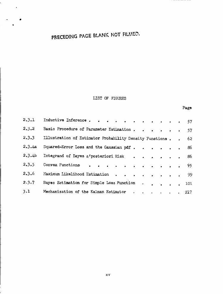
LIST OF FIGURES
Inductive Inference ..........
Basic Procedure of Parameter Estimation .....
Illustration of Estimator Probability Density Functions .
Squared-Error Loss and the Gaussian pdf .....
Integrand of Bayes a'posteriori Risk .....
Convex Functions ..........
_xinann Likelihood Estimation .......
Bayes Estimation for Simple Loss Function• • e
Mechanization of the Kalman Estimator
Page
• 57
• 57
. 62
. 86
• 86
. 95
• 99
. lO1
• 217
XV
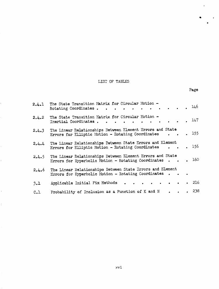
LIST OF TABLES
Page
2.H.I
2.H.2
2.H.3
2.H.J+
2.1+.5
2.H.6
The State Transition ;_trix for Circular Motion -
Rotating Coordinates ..........
The State Transition }_trixfor Circular Motion -
Inertial Coordinates ..........
The Linear Relationships Between Element Errors and State
Errors for Elliptic }_tion - Rotating Coordinates . •
The Linear Relationships Between State Errors and Element
Errors for Elliptic Motion - Rotating Coordinates . .
The Linear Relationships Between Element Errors and State
Errors for H_erbolic Motion - Rotating Coordinates . .
The Linear Relationships Between State Errors and Element
Errors for Hyperbolic Motion - Rotating Coordinates . .
Applicable Initial FixMethods .......
Probability of Inclusion as a Function of K and N . .
• IA7
. 155
• 156
. 160
• 216
. 238
xvi
1.O STATEMENTOFTHEPROBLEM
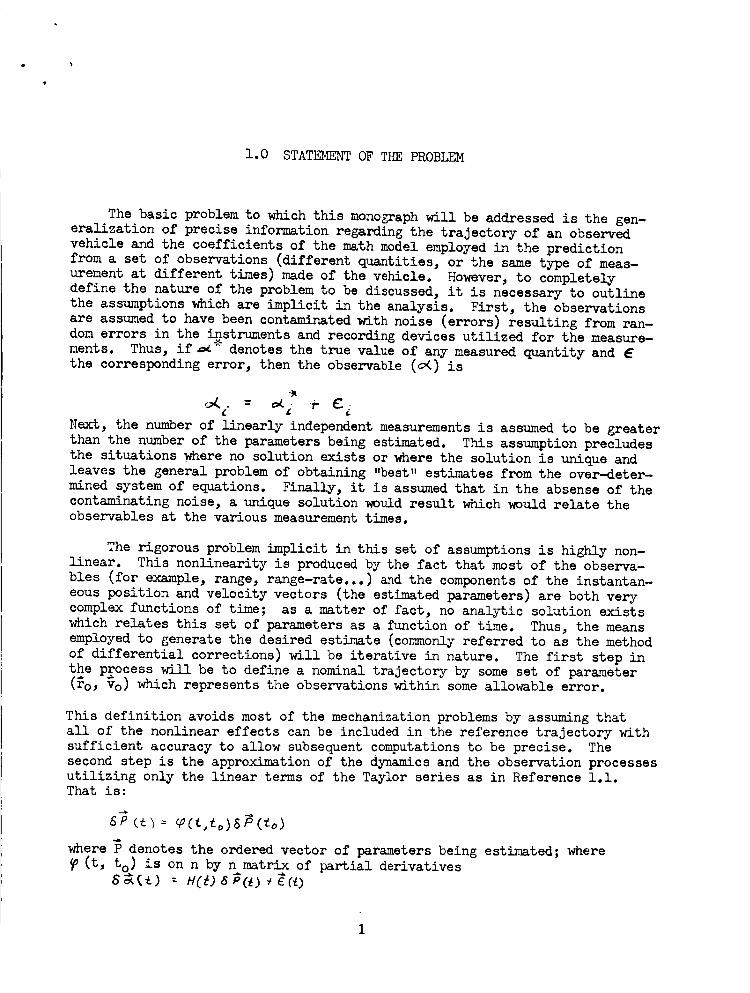
The basic problemto which this monographwill be addressedis the gen-eralization of precise information regarding the trajectory of an observedvehicle and the coefficients of the mathmodel employedin the predictionfrom a set of observations (different quantities, or the sametype of meas-urement at different times) madeof the vehicle. However,to completelydefine the nature of the problem to be discussed, it is necessary to outlinethe assumptionswhich are implicit in the analysis. First, the observationsare assumedto have been contaminatedwith noise (errors) resulting from ran-domerrors in the instruments and recording devices utilized for the measure-ments. Thus, if_* denotes the true value of any measuredquantity andthe corresponding error, then the observable (_) is
Next, the numberof linearly independentmeasurementsis assumedto be greaterthan the numberof the parametersbeing estimated. This assumptionprecludesthe situations whereno solution exists or where the solution is unique andleaves the general problemof obtaining "best" estimates from the over-deter-mined system of equations. Finally, it is assumedthat in the absenseof thecontaminating noise, a unique solution would result which would relate theobservables at the various measurementtimes.
The rigorous problem implicit in this set of assumptions is highly non-linear. This nonlinearity is producedby the fact that most of the observa-bles (for example, range, range-rate...) andthe componentsof the instantan-eous position and velocity vectors (the estimated parameters) are both verycomplexfunctions of time; as a matter of fact, no analytic solution existswhich relates this set of parameters as a function of time. Thus, the meansemployedto generate the desired estimate (commonlyreferred to as the methodof differential corrections) will be iterative in nature. The first step inthe process will be to define a nominal trajectory by someset of parameter(_o, to) which represents the observationswithin someallowable error.
This definition avoids most of the mechanization problemsby assumingthatall of the nonlinear effects can be included in the reference trajectory withsufficient accuracy to allow subsequentcomputationsto be precise. Thesecondstep is the approximation of the dynamicsand the observation processesutilizing only the linear terms of the Taylor series as in Reference1.1.That is:
where_ denotes the ordered vector of parameters being estimated; where
(t, to) is on n by n matrix of partial derivatives
l
of the parameters at time t with respect to the same set of parameters at
time to_ where H(t) is the matrix of partial derivatives of the observables
with respect to the parameters being estimated at the epoch of the observa-
tion_ and where _ (t) is the vector of errors in the true observables.
Finally estimates of the parameters at some selected epoch (T) will be
generated. These estimates will be selected such that some measure of
"goodness" in the estimator is maximized when the available information
regarding the statistics of the errors is provided.
The discussions of this monograph will be ordered to answer questions
which arise regarding each of the steps in this process and will relate in
detail the nature of the problem. To accomplish this objective, large amounts
of the open literature have been reviewed. Though this material is generally
referenced throughout the text to provide additional information on topics
being discussed, some of the more pertinent references will be quoted in the
following paragraphs to aid in establishing the nature of the discussions.
The initial investigations will be directed to the task of generating a
reliable first approximation to the true trajectory. This step will be per-
formed by utilizing the material presented in a previous monograph (Ref. 1.3)
and classical work, principally of Laplace and Gauss. In this material, the
true trajectory is approximated by a nearly equivalent conie section to obtain
the position and velocity vectors which, if the force field were central,
would yield the subset of the observables used to define the conic section.
The solution is discussed in detail and precautionary steps which will assume
more reliable solutions are presented. Thus, if no previous estimate of the
trajectory or data from the vehicles guidance system at burnout are available,
an accurate initial estimate can be generated.
The discussions will then turn to the development of the "optimum" esti-mates of the deviation vector _(t). Particular attention will center on the
development of simple measures of the degree of optimality in the estimator
and the generation of the estimation equations and estimation error for these
measures. These discussions will parallel much of the material presented in
the open literature, though some of the steps are different to facilitate
comprehension of the simplest physical process. The classical least squares,
weighted least squares, and minimumvariance estimators will be derived; then
attention will turn to modern estimation in a recursive mode. The concepts
of Kalman as presented in Reference O.1 (subsequently adopted by Schmidt in
Reference 0.2) and Battin (Reference 0.3) will be reviewed carefully since
estimation in this mode is capable of correcting for some of the approxima-
tionsmade in developing the estimator itself. This latter observation is the
result of the fact that the true trajectory (i.e., nonlinear) can be approxi-
mated by a series of discontinuous arcs, each of which obeys the linear model
of the dynamics, to a better degree than a single arc satisfying the same
linear model.
The filter concepts outlined in the previous paragraph are based on intu-
itive measures of "optimality." Further, they are tailored to problems where
the statistics involved are Gaussian, where the dynamics can be adequately
approximated by the linear model, and where the optimum estimator is a linear
function of the deviations in the observables. Thus, the problem of estimationis reintroduced in a morecomplete analysis to explain the exact nature ofthe material which it follows, and to demonstratethe mechanismwherebysomeof the simplifications just enumeratedcanbe eliminated. In the process, theproblem is demonstratedto be equivalent to that presented by _ddleton inReference 0._. This material, while requiring a reasonable knowledgeofstatistical concepts, ties the general estimation problem into a verifiedanalytic frameworkwhich is capable of demonstrating the effects of the avail-ability of all data pertaining to the process.
Having thoroughly explored the general problem of estimation, attentionturns to the developmentof material required to yield an estimate of thetrajectory. To be specific, the matrices relating the dynamicsat varioustimes relative to the nominal trajectory (the State Transition _trix denoted
by _(t, to) and the matrix presenting the error data for the observables are
derived. The first of these developments progresses from the basic formula-
tion of the transition matrix (for example, Reference 0.5) to the generation
of an analytic form for the case of conic motion (for example, References
0.6, 0.7, 0.8, 0.9). This development presents several alternate representa-
tions of the desired matrix and discusses the weaknesses in them. The second
development is an extension of the material presented in a previous monograph
(Reference 1.1) which shows the functions involved in the process and refers
to error data available in the literature for construction of the weightingmatrix.
The monograph concludes with a set of recommendations for the applica-
tion of this materialand one possible mechanization whichwill be selected toutilize the maximum amount of information in the data and to minimize the
computational problems.
3
2.0 STATE OF THE ART
2.1 INITIAL ESTIMATES OF THE ORBIT
Since the computational rationale proposed for determining precise
values of the instantaneous elements for the space trajectory is built upon
the concept of differential corrections, care must be exercised to assure
that the initial estimates of the nominal trajectory are sufficiently precise
to allow all of the partial derivatives to be evaluated accurately and to
assure that the estimation error lies within the neighborhood about the
true trajectory which is small enough for the process to converge. The
purpose of this discussion will be to develop several such techniques andto discuss the sources of error. To be specific, the methods of Laplace
and Gauss as well as methods involving the use of range and range-rate data
wdll be presented in detail. The utilization of position and velocityinformation obtained directly from an integrating accelerometer (Reference
i.i) will not be discussed at this time since this information can be
be utilized only for those cases in which the trajectory is to be estimated
from the epoch of injection to any other reference epoch (any other possibility
requires updating burnout conditions to the epoch of problem initiation) and
since the data thus provided need no further transformation (i.e., they can
be utilized directly if transmitted to the ground or fed to the on-board
computer).
2.1.1 Data Provided Include Range_ Azimuth and Elevation at Two Epochs
For the case in which the ground-based radar utilized for tracking the
satellite provides range, azimuth and elevation (or an equivalent set of data)
as a function of time, the logic employed to obtain an estimate of the tra-
jectory can be relatively simple. First, the station's position at the two
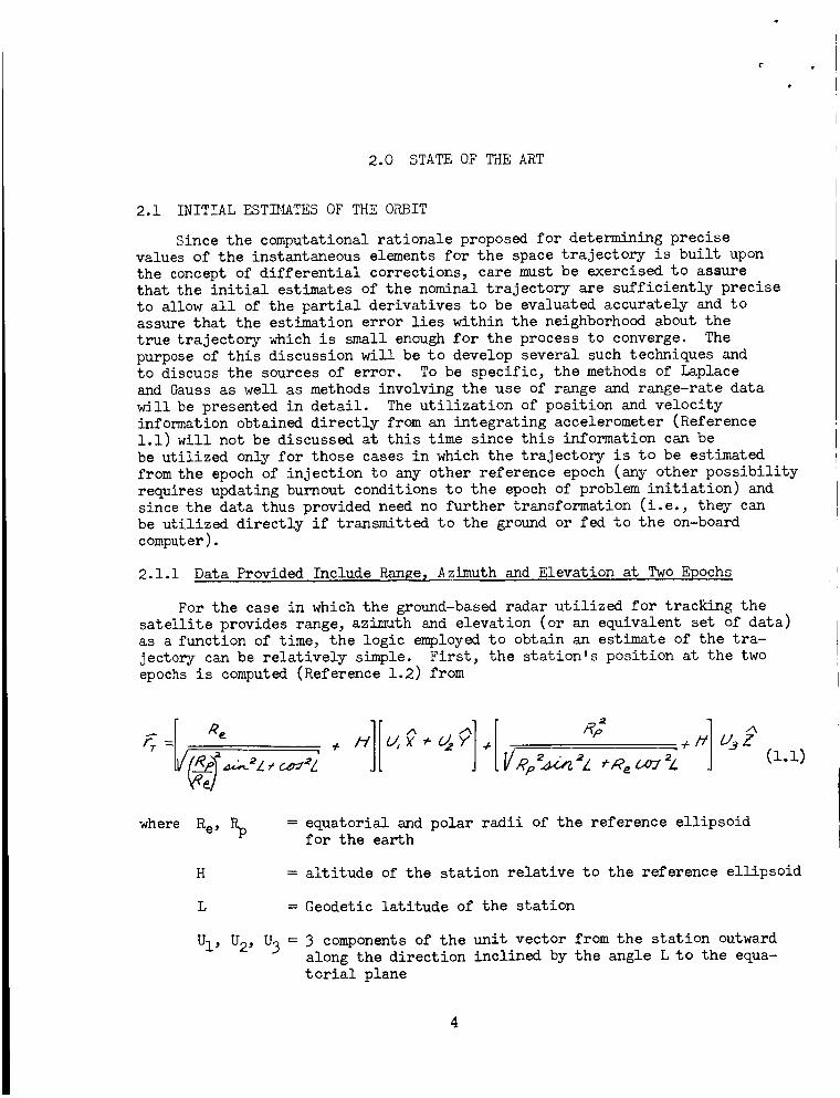
epochs is computed (Reference 1.2) from
(i.i)
where Re, = equatorial and polar radii of the reference ellipsoidfor the earth
H = altitude of the station relative to the reference ellipsoid
L = Geodetic latitude of the station
UI, U2, U3 = 3 components of the unit vector from the station outwardalong the direction inclined by the angle L to the equa-
torial plane
4
i-, /k /_
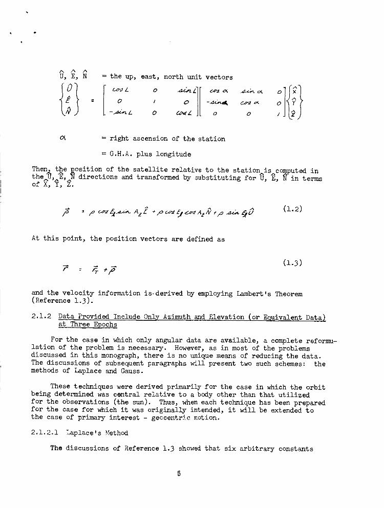
U, E, N = the up,
_L
= 0
east, north unit vectors
0 _c_ _c_ c_ o X
J -_ c_ o_ o
o _.,wZ JL o o /
c_ = right ascension of the station
= G.H.A. plus longitude
Then. the Position of the satellite relative to the station is computed inthe _, _, _ directions and transformed by substituting for 9, E, _ in terms
(l.2)
At this point, the position vectors are defined as
r : _ +p(1.3)
and the velocity information is. derived by employing Lambert's Theorem(Reference 1.3).
2.1.2 Data Provided Include Only Azimuth and Elevation (or Equivalent Data)at Three Epochs
For the case in which only angular data are available, a complete reformu-
lation of the problem is necessary. However, as in most of the problems
discussed in this monograph, there is no unique means of reducing the data.
The discussions of subsequent paragraphs will present two such schemes: the
methods of Laplace and Gauss.
These techniques were derived primarily for the case in which the orbit
being determined was central relative to a body other than that utilized
for the observations (the sun). Thus, when each technique has been prepared
for the case for which it was originally intended, it will be extended to
the case of primary interest - geocentric motion.
2.1.2.1 Laplace's Method
The discussions of Reference 1.3 showed that six arbitrary constants
were required to uniquely determine the motion of a body in a central forcefield. Thus, if the true force field is approximatedby that produced bythe dominantmass(or in the case of motion relative to the earth, by thatproducedby neglecting those terms arising from the nonspherical shapeof the earth), a conic trajectory can be found utilizing three sets ofobservations composedof angular data (azlmuth-elevation, right ascension-declination, etc. ).
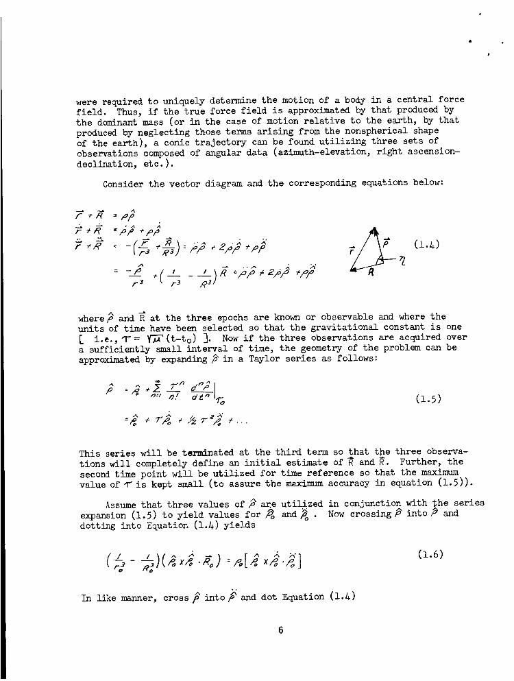
Consider the vector diagram and the corresponding equations below:
f _R =PF
r +R = ÷pp
f+,E' =• .o
=>? 2?? +pp
= +( ,f 3 1.-3
___ (1._)
where _ and _ at the three epochs are known or observable and where the
units of time have been selected so that the gravitational constant is one
i.e., _N= _-_ (t-to) _. Now if the three observations are acquired over
a sufficiently small interval of time, the geometry of the problem can be
approximated by expanding _ in a Taylor series as follows:
"-p_ +'r'_ +_?-_ ÷...
(1.5)
This series will be terminated at the third term so that the three observa-
tions will completely define an initial estimate of _ and _. Further, the
second time point will be utilized for time reference so that the maximum
value orris kept small (to assure the maxinmm accuracy in equation (1.5)).
Assume that three values of_ a_e utilized in conjunction with the series
expansion (1.5) to yield values for _ and_ . Now crossing_into _ and
dotting into Equation (1._) yields
In like manner, cross _ into _ and dot Equation (1.&)
(1.8)
/
R,." ¢.x_. = 2 .fl.x._..(1.7)
Now the procedure is to iterate Equation (1.6) and the law of cosines
:=N-R
or
(l.8)
to solve for the correct value of _rl at._o._ This value of r can then beutilized in Equation (1.7) to solve for Po; ro can be found from
-..,_o_->o,_,:o_
The nature of the simultaneous solution of Equations (1.6) and (1.8)
is explored in some detail in Reference 1.&. This material develops an
iteration procedure based on a single angular variable. The result of this
procedure is an iteration process which can rely on graphical techniques for
initial estimates of the parameter being estimated.
If the central body is the earth rather than the sun, differences in theformulation arise due to the fact that the acceleration of the observer is
incorrect. For this case
_ - "'(7_)-dL 2
and Equation (1.6), which was solved iteratively with the law of cosines,becomes
('%,,,,)(,.,:,._)= ,.[_.,,..4] .Similarly, Equation (1.7), which was solved for Jo , becomes
(1.6a)
( )(_ ) >.[" "]__/ x -. = -z p. x_.,_. (l.Ta)f2 * ..,2 x/% ._o
The largest source of error in the process is the truncation of Equa-
tion (1.5) at the third term. This step means that the values of _o and Vo
which are obtained from the process will not represent the conic providingthe three observations to the best degree. Thus, it is generally desirableto differentially correct the_vectors before assumingthat a solution isknown. This process is readily accomplishedutilizing the material pre-sented in Section 2._ of this monographsince
and
(1.9)
y,4 =Hz x(1.1o)
where a_ = a vector of observed minus computed residuals at the three
epochs (1-1, V2, T"3 )
H = the matrix relating errors in the observables to small errors
in the position and velocity
A_ = a vector of position and velocity deviations (d?, d_)
Thus, the vector of errors at the epoch _2 (A_o) can be estimated as
and the previously computed values of 3 o
to= ro + ar_
Vo = Vo + a
(l.lla)
and Vo corrected
(1.11b)
(1.11c)
This second estimate of r_o, T o can now be utilized to generate a new error
vector (a_) so that the process can continue until convergence is achieved.
2.1.2.2 Gauss's Method
In Laplace's method, the approximations made to facilitate the solutionwere in the truncation of the Taylor series for _. Gauss approached the
problem bymaking an approximation in the dynamics rather than in the geometry.
The method proceeds as follows: Since the motion is assumed planar, any
of the three radii can be expressed as some linear function of the other
two, i.e.,
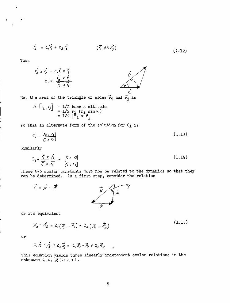
q "- c,r,+ c 3 6 #i<(i.12)
Thus
qx6 : c,r,× ra.__% ._.%
r,×q__.%
But the area of the triangle of sides ri and _j is
A--[_>O] = 1/2 base x altitude= 1/2 ri (ri sin_)
= 1/21_ i x _jl
so that an alternate form of the solution for Cl is
c, _ (1.13): ?,, ,]]
Similarly
c3-__ x __ _ [_,, _] (1._)
These two scalar constants must now be related to the dynamics so that they
can be determined. As a first step, consider the relation
--_ __% ___
r. =p -,6:'
or its equivalent
(i.15)
or
This equation yields three linearly independent scalar relations in the
unknowns c,,¢3 )_(,_: 1,3) .
i
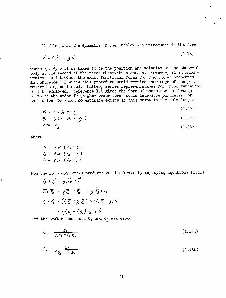
At this point the dynamics of the problem are introduced in the form
(1.16)
where To, _o will be taken to be the position and velocity of the observed
body at the second of the three observation epochs. However, it is incon-venient to introduce the exact functional forms for f and g as presented
in Reference 1.3 since this procedure would require knowledge of the para-
meters being estimated. Rather, series representations for these functions
v_ll be employed, reference 1.& gives the form of these series throughterms of the order T2 (higher order terms would introduce parameters of
the motion for which no estimate exists at this point in the solution) as
(l.17a)&.: , - _ _D _
3_= p (,-y,_-p,) (i.I_o)
_: >_Z (1.17c)
where
_= v-_- (% - <)_= _,/-_--( % - _,)
Now the follo_lng cross products can be formed by employing Equations (1.16)
r_× 6 =93r2 xr_
r,_ = 9,_ ×_= -2'0_
and the scalar constants C1 and C3 evaluated.
9_ (1.isa)c_, : -D_.,- 6 _,,
c3 : -_' (l.18b)r,_ -_ a,
10
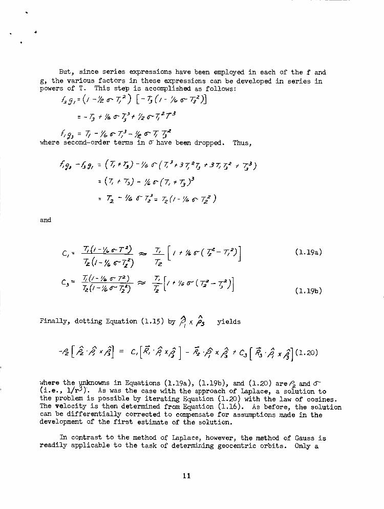
But, since series expressions havebeen employedin each of the f andg, the various factors in these expressions can be developed in series inpowers of T. This step is accomplishedas follows:
-__ +_o'-_'+ y2o-,-_T 3
D_,_-- _ - yo _ _ _- _ o" 7; _ "_where second-order terms in _ have been dropped. Thus,
and
C = 7;(/-Y_,¢'T_.) _ _ [
C3= _ (I '.,'c,6- 7_) _ I
(1.19a)
(1.19b)
Finally, dotting Equation (1.15) by X p_ yields
where the unknowns in Equations (1.19a), (1.19b), and (1.20) are_ and o_(i.e., l/r3) '. As was the case with the approach of laplace, a solution to
the problem is possible by iterating Equation (1.20) with the law of cosines.
The velocity is then determined from Equation (1.16). As before, the solution
can be differentially corrected to compensate for assumptions made in thedevelopment of the first estimate of the solution.
In contrast to the method of laplace, however, the method of Gauss is
readily applicable to the task of determining geocentric orbits. Only a
11
r
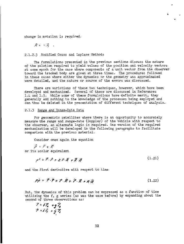
change in notation is required.
_= -77
2.1.2.3 Modified Gauss and Laplace Methods
The formulations presented in the previous sections discuss the nature
of the solution required to yield values of the position and velocity vectors
at some epoch for the case where components of a unit vector from the observer
toward the tracked body are given at three times. The procedures followed
in these cases where either the dynamics or the geometry was approximated
were detailed, and the nature or source of the errors was discussed.
There are variations of these two techniques, however, which have been
developed and mechanized. Several of these are discussed in References1.A and 1.5. While some of these formulations have definite merit, they
generally add nothing to the knowledge of the processes being employed and
can thus be deleted in the presentation of different techniques of analysis.
2.1.3 Range and Range-Rate Data
For geocentric satellites where there is an opportunity to accurately
measure the range and range-rate (Doppler) of the vehicle with respect to
the observer, an alternate logic is required. One version of the required
mechanization ;_lll be developed in the following paragraphs to facilitate
comparison with the previous material.
Consider once again the equation
or its scalar equivalent
: z (1.21)
and the first derivative with respect to time
(1.22)
But, the dynamics of this problem can be expressed as a function of time
utilizing the f, g series (as was the case before) by expanding about thesecond of three observations as:
?=r?o•
12
Thus,
_ _ = ri_',_ t,Cr],2i),26v_
F. = _r,. ,_ ro.R
• i_ 24r "R = .R , .R
r.,e =r_._ +2 r. .R
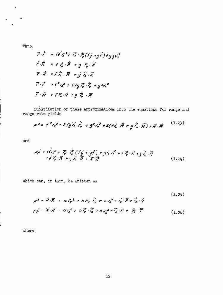
Substitution of these approximations into the equations for range andrange-rate yields
(1.23)
and
(_.m)
which can, in turn, be written as
,_- ,_._"
(1.25)
where
• °
13
@
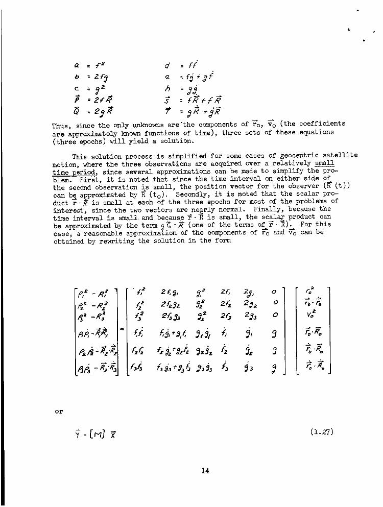
= _z d -- ,"/
-_ ..h
=2 R =f = R+
Thus, since the only unknowns are'the components of r-_o,v_ (the coefficients
are approximately known functions of time), three sets of these equations
(three epochs) will yield a solution.
This solution process is simplified for some cases of geocentric satellite
motion, where the three observations are acquired over a relatively small
time periqd, since several approximations can be made to simplify the pro-blem. First, it is noted that since the time interval on either side ofthe second observation is small, the position vector for the observer (_ (t))
can be a_proximated by H (to). Secondly, it is noted that the scalar pro-duct r _ is small at each of the three epochs for most o£ the problems of
interest, since the two vectors are ne.arly normal. Finally, because the
time interval is small and because _-_ is small, the scala_ product can
be approximated by the term _ "_ (one of the terms of _ R). For this
case, a reasonable approximation of the components of _o and _o can be
obtained by rewriting the solution in the form
p,_ -Rf
.
-R,.R,
"_',_ 2_,g, ,e) z_, zj, o
or
(1.27)
14
@
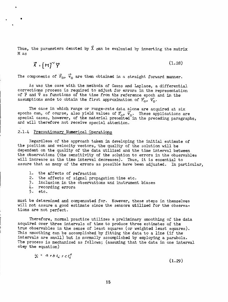
Thus, the parameters denoted by X can be evaluated by inverting the matrix
M as
The components of ro, vo are then obtained in a straight forward manner.
As was the case with the methods of Gauss and Laplace, a differential
corrections process is required to adjust for errors in the representation
of _ and V as functions of the time from the reference epoch and in the
assumptions made to obtain the first approximation of r-_o,v_.
The case in which range or range-rate data alone are acquired at six
epochs can, of course, also yield values of r_o, _o" These applications are
special cases, however, of the material presented in the preceding paragraphs,
and will therefore not receive special attention.
2.1._ Precautionary Numerical Operations
Regardless of the approach taken in developing the initial estimate of
the position and velocity vectors, the quality of the solution will be
dependent on the quality of the data utilized and the time interval between
the observations (the sensitivity of the solution to errors in the observables
will increase as the time interval decreases). Thus, it is essential to
assure that as many of the errors as possible have been adjusted. In particular,
1. the affects of refraction
2. the affects of signal propagation time etc.3. inclusion in the observations and instrument biases
i. recording errors5. etc.
must be determined and compensated for. However, these steps in themselves
will not assure a good estimate since the sensors utilized for the observa-
tions are not perfect.
Therefore, normal practice utilizes a preliminary smoothing of the data
acquired over three intervals of time to produce three estimates of the
true observables in the sense of least squares (or weighted least squares).This smoothing can be accomplished by fitting the data to a line (if the
intervals are small) but is normally accomplished by employing a parabola.
The process is mechanized as follows; (assuming that the data in one interval
obey the equation)
(1.29)
15
where Yi = ith observed value of one component of the observationvector in the interval A_ t _B
a, b, c = coefficients of parabola utilized for the purposes of
smoothing the data
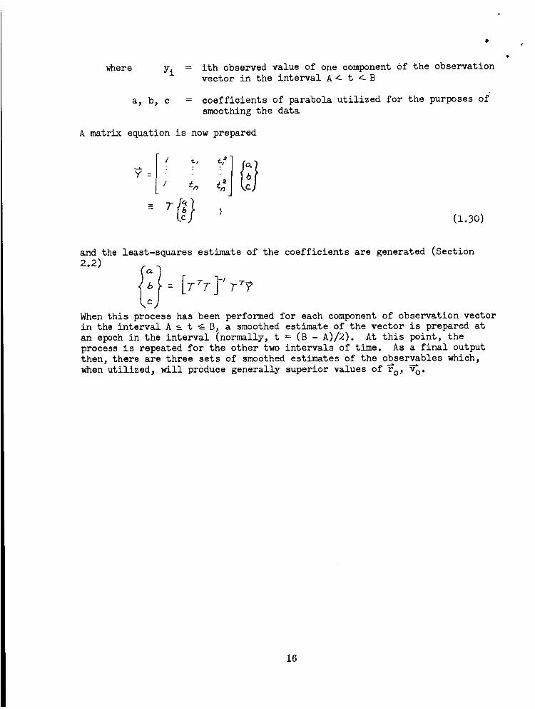
A matrix equation is now prepared
Y=
/ _, _fl (it
(1.30)
o
and the least-squares estimate of the coefficients are generated (Section
2.2)
= TT_
When this process has been performed for each component of observation vector
in the interval A _ t _ B, a smoothed estimate of the vector is prepared at
an epoch in the interval (normally, t = (B - A)/2). At this point, the
process is repeated for the other two intervals of time. As a final output
then, there are three sets of smoothed estimates of the observables which,
when utilized, will produce generally superior values of r_o, _o"
16
2.2 ORBIT IMPROVEMENT
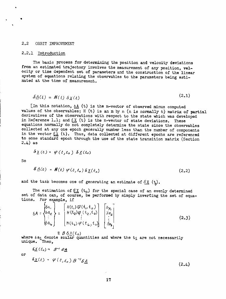
2.2.1 Introduction
The basic process for determining the position and velocity deviations
from an estimated trajectory involves the measurement of any position, vel-ocity or time dependent set of parameters and the construction of the linear
system of equations relating the observables to the parameters being esti-mated at the time of measurement.
JX_Ct) = HCf) 6__C_) (2.1)
[In this notation, ___A(t) is the m-vector of observed minus computed
values of the observables; H (t) is an m by n (n is normally 6) matrix of partial
derivatives of the observations with respect to the state which was developedin Reference i.i; and g__X(t) is the n-vector of state deviations. These
equations normally do not completely determine the state since the observables
collected at any one epoch generally number less than the: number of components
in the vector ___X(t). Thus, data collected at different epochs are referenced
to some standard epoch through the use of the state transition matrix (Section2._) as
So
(2.2)
and the task becomes one of generating an estimate of 6X (_.
The estimation of 6__X (to) for the special case of an evenly determined
set of data can, of course, be performed by simply inverting the set of equa-
tions. For example, if
I ](2.3)
where _a i denotescalar quantities and where the ti are not necessarilyunique. Then,
or
(2._)
17
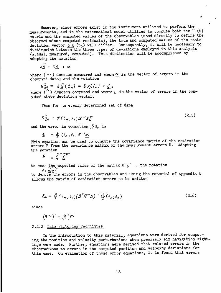
However,since errors exist in the instrument utilized to perform themeasurements,and in the mathematical model utilized to computeboth the H (t)matrix and the computedvalues of the observables (used directly to define theobservedminus computedresiduals), the true and computedvalues of the statedeviation vector g___X(to) will differ. Consequently, it will be necessary todistinguish betweenthe three types of deviations employedin this analysis(actual, measured,computed). This distinction will be accomplishedbyadopting the notation
where (N) denotes measuredand where--_is the vector of errors in theobserveddata; and the notation
where (^) denotes computedand whereE is the vector of errors in the com-puted state deviation vector.
Thusfor _ evenly determined set of data
and the error in computing____ is
This equation can be used to computethe covariance matrix of the estimationerrors E from the covariance matrix of the measurementerrors R. Adoptingthe notation
to meanthe expectedvalue of the matrix£ _T , the notation
to denote the errors in the observables and using the material of AppendixAallows thematrixof estimation errors to be written
$
(2.6)
since
-(mS)-'
2.2.2 Data Filterin_ Techniques
In the introduction to this material, equations were derived for comput-
ing the position and velocity perturbations when precisely six navigation sight-
ings were made. Further, equations were derived that related errors in the
observations to errors in the computed position and velocity deviations for
this case. On evaluation of these error equations, it is found that errors
IB
in the observables of relatively small magnitudescan produce errors in thecomputedposition perturbations that are completely unacceptable. Thequestion then arises as to howadditional sighting might be used to obtaina better estimate. Several methodsof accomplishing this objective will beconsidered.
However,before considering this material it will be noted that any orall of the various estimation processes canbe employed. The choice, shouldhowever, dependon the amountof information kno_nabout the errors in theobservables. Thus, attempts will be madeto demonstratethe accuracy (estima-tion error) of each approachand to explain the differences in precisionobtained in terms of the assumptionsmadein deriving the estimator. In allcases, however, the assumptionof secondorder statistical distributions isimplicit (the discussions repeatedly employAppendixA). Thus, informationpertaining to higher momentsis not employedand the "goodness" of the estimatorshould be suspect for non-Gaussianerrors.
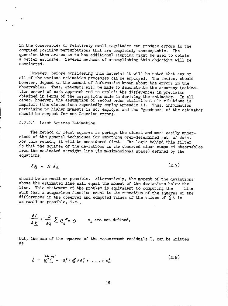
2.2.2.1 Least SquaresEstimation
The methodof least squares is perhapsthe oldest and most easily under-stood of the general techniques for smoothingover-determined sets of data.For this reason, it will be considered first. The logic behind this filteris that the squares of the deviations in the observedminus computedobservablesfrom the estimated straight line (in m-dimensionalspace) defined by theequations
should be as small as possible. Alternatively, the momentof the deviationsabovethe estimated line will equal the momentOf the deviations below theline. This statement of the problem is equivalent to computingthe linesuch that a comparisonfunction equal to the summationof the squares of thedifferences in the observedand computedvalues of the values of _ A isas small as possible, i.e.,
J42_=--'- e.=o ei are not defined.
But, the sum of the squares of the measurement residuals L, can be writtenas
19
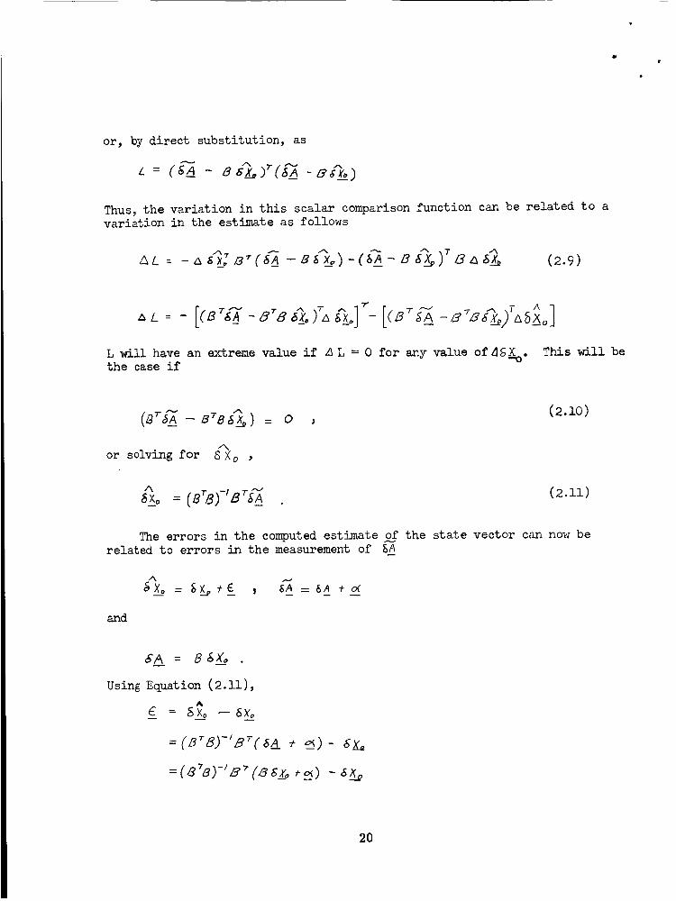
or, by direct substitution, as
Thus, the variation in this scalar comparison function can be related to avariation in the estir_te as follows
L will have an extreme value if D L = 0 for any value of 4gX_o. This will bethe case if
ik
or solving for 8Xo ,
A
= (a,8)-,aTG_
(2.lO)
(2.1i)
The errors in the computed estimate of the state vector can now berelated to errors in the measurement of SA
_Xo = gD t-_£ _ _A = 6A • o¢
and
sA = 8_
Using Equation (2.11),
= (a_)-'_(__ _ _)- _
= (_b)-'_ _(a_,o, __)- ___o
20
Then
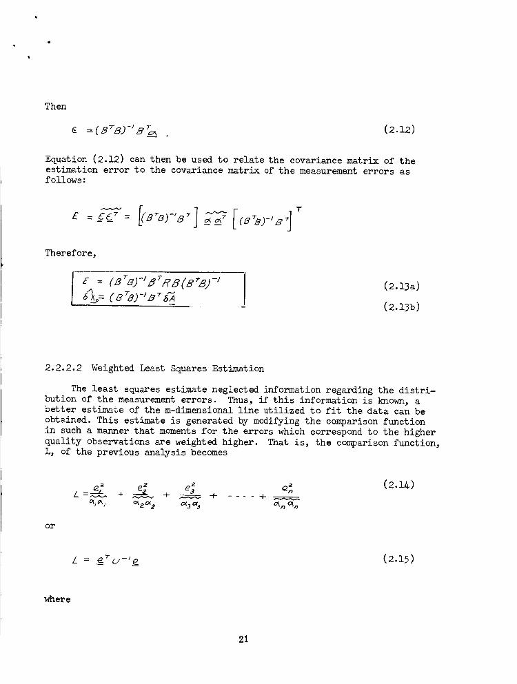
=(a_8)-'sh (2.12)
Equation (2.12) can then be used to relate the covariance matrix of the
estimation error to the covariancematrixof the measurement errors asfollows:
g =-C£_- = 8_B) -'B_ _'_ 8 -'B
Therefore,
E.,= Ca_8)-,B_Ra(8_a)-,_ ] (2.13a)
2.2.2.2 Weighted Least Squares Estimation
The least squares estimate neglected information regarding the distri-
bution of the measurement errors. Thus, if this information is known, abetter estimate of the m-dimensional line utilized to fit the data can be
obtained. This estimate is generated by modifying the comparison function
in such a manner that moments for the errors which correspond to the higher
quality observations are weighted higher. That is, the comparison function,L, of the previous analysis becomes
or
_ , _ (2.11,)£= + e.._2 + _e 3 + .... + _%_ ¢_zcx2 c_a % o_n c_n
/ = _(u-'_ (2.15)
where
21
e _
A
"_ 0 0
_' _ II _- 2
J 0 \ I
I I \ iI I
\ 0
0 0 0 a_ _n
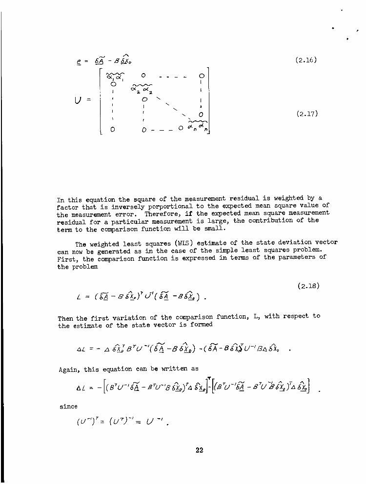
(2.16)
(2.17)
In this equation the square of the measurement residual is weighted by a
factor that is inversely porportional to the expected mean square value of
the measurement error. Therefore, if the expected mean square measurement
residual for a particular measurement is large, the contribution of the
term to the comparison function will be small.
The weighted least squares (WIS) estimate of the state deviation vector
can now be generated as in the case of the simple least squares problem.
First, the comparison function is expressed in terms of the parameters of
the problem
7 N A
(2.1_)
Then the first variation of the comparison function, L, with respect to
the estimate of the state vector is formed
Again, this equation can be written as
aL = - (B'U-'6"A-e_O-'86_)a - _U-'5_-B'O'B6L)'a__
since
(u-') u-'
22
But, since both of the terms of this equation are scalars, the transpose
of the bracketed term is equal to itself. This fact indicates that the loss
function will have a stationary value when the estimate is chosen so that
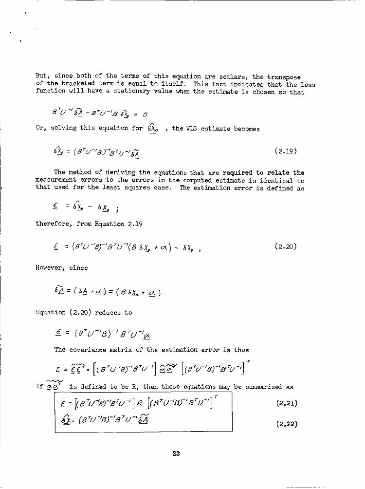
Or,
A
solving this equation for g_o , the WIS estimate becomes
The method of deriving the equations that are required to relate the
measurement errors to the errors in the computed estimate is identical to
that used for the least squares case. The estimation error is defined as
therefore, from Equation 2.19
However, since
Equation (2.20) reduces to
The covariance matrix of the estimation error is thus
If _m__T is defined to be R, then these equations may be summarized as
_: 7_<,,-,_r,,_<,,-,],_[cB.u-,_;,_u-,]_ (_._)_: (_Tu-'sJ-'8"u-'_-- (2.22)
23
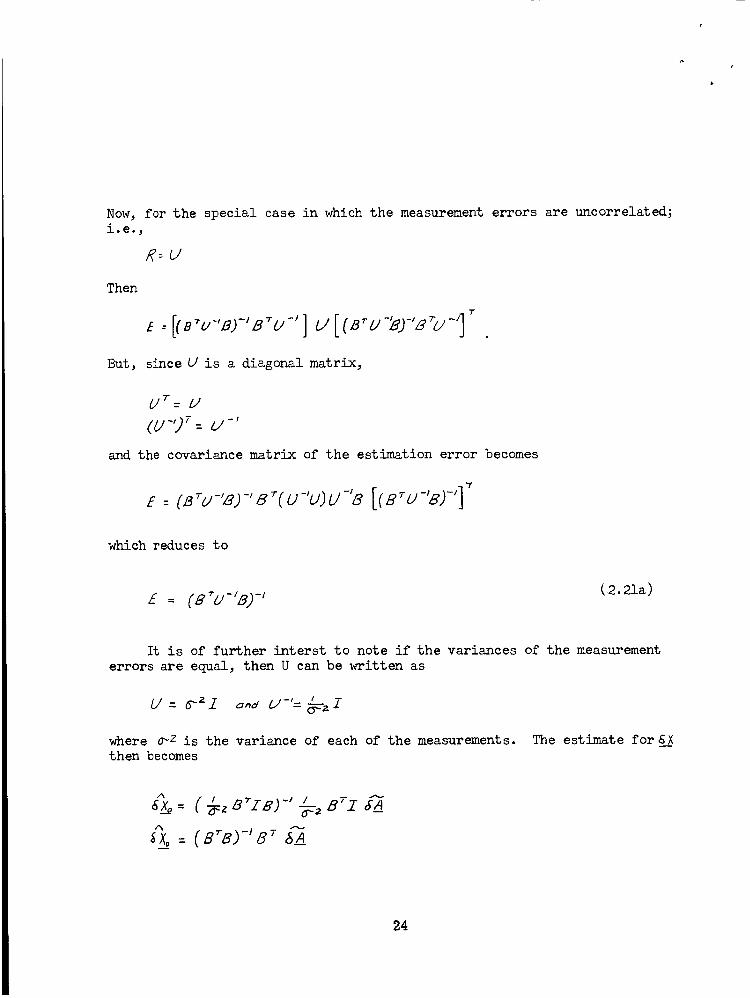
Now, for the special case in which the measurement errors are uncorrelated;
i.e.,
Then
R=U
,]But, since U is a diagonal matrix,
UT= I_."
Cu 97= d-'
and the covariance matrix of the estimation error becomes
E - (_u-'_)-'8"(u-'u)u-'8 [(e_u-'e)-']"
which reduces to
z : (_u"8)-'[2.21a)
It is of further interst to note if the variances of the measurement
errors are equal, then U can be written as
L/ : 6"zZ o_d U-': 'o_---zi
where 0_z is the variance of each of the measurements. The estimate for 6__X
then becomes
_Xo=('_ -_zS_IB) "' '-_2 8TI &A
*% ( -2 T
94
This equation indicates that for the case in which the variances of the
measurement errors are equal the weighted least squares estimate will reduce
to the least squares estimate.
2.2.2.3 Minimum Variance Estimation
In developing the estimation equations for both the least squares
and the weighted least squares filters, a loss function was utilized which
was simply related to the moments of the errors. The estimation equationwas then formulated to minimize this loss function. In neither case was
the statistical information pertaining to correlations in the components
of the error vector ( _ ) utilized. Thus, at this point a different approach
to the problem will be formulated. To be specific, that estimate (definedas optimum) of the state deviation vector which is a linear function of the
measurements, which minimizes each element of the estimation error covariance
matrix and which corresponds to the constraint that the estimation error is
not influenced by the quantity being estimated will be developed. That is,the form of the estimate is to be
2% N
6XD = Q 6A(2.23)
But,
Thus, by direct substitution,
(2.24)
so that the error in the estimate is
This equation indicates that if the error in the estimate is to be independent
of the quantity being estimated, 5Xo, it is necessary that
Oz_-_T = 0(2.26)
25
The estimation error then becomes
§o = Q___
and the estimation error covariance matrix becomes
CoC_ = 0___ _
or defining
f : q_ 7
(2.27)
The problem now is to determine Q such that it will minimize E subject
to the constraint that
08-I :o
This step can be accomplished by adjoining the constraint equation to E using
matrix Lagrange multipliers as follows. Since
QB-I = o , GrQ_-I= O
4),9'/ -A = ,\_BTQ T- A T = O
(2.28)
where k is an arbitrary n by n matrix multiplier that is not a function of
Q. Thus
T
F : E, +
=ORQ _ _ 00A _ A_8_T-A -A.
(2.29)
Now, recalling that RT- R, the first variation of F ( : F) becomes
26
But the 8@ are arbitrary.extremevalue if
or
R,_T,"BA = 0
QT =_ R-'SA .
Therefore, each element of E will have an
(2.3o)
(2.31)
Thus,
But
thus_
premultiplying by BT yields
8_ _ = -_R-'s_.
B_4 _T = Z j
A =- ('B"R-_J -I (2.32)
so that
and
a =CB m- j-'B m-' (2.33b)
since both R and (_,_-J B)
estimation equation isare sy_netric. Thus, the minimum variance
It is interesting to note that when the errors in the measurements are
uncorrelated (i.e., R = U), the minimum variance and weighted least squaresestimates are identical.
27
Equations (2.27), (2.33a), and (2.33b) can be used to express theerrors in the estimate as follows:
(.B -,8j-I
therefore, in summary
f -- (2.35)
(2.36)
In the development of these equations, Q was constrained to make E
invariant with respect to the characteristics of g Xo Thus, these
equations should be used to estimate 8_o when the statistical characteristicsof 6Xo are m3.k_own. However, when the statistical characteristics of _o
are known, that is, if the covariance matrix of S_o is known, this con-
straint should be removed. _Cnen this is done, the resulting estimation
equation can be determined as follows. From Equation (2.25)7
Now, defining
and rewriting the estimation error yields
E = _[BVSTJ-/_JQ_-@_'V-I/'Sz@-zj. V (2.37)
The variation in E that is produced by a variation in Q is thus
28
is to be zero for the case where
+R)qR SV= o ;
S Q is arbitrary
(2.3s)
that is, E will have an extreme value if
Qz= ('8 VB T+ R)-'SV (2.39a)
Thus
since R = RT and V = VT.
The optimum estimate is now found by substitution into Equation (2.23)
A .v (2._o)6_Xo = VB "(B V'8 T+R) -/ 6A
The error in the estimate is determined using Equations (2.37) and (2.39b)as
E = vz3rq_ -Qsv- vs_q_+v .
Thus summarizing,
E = v- V_"(MV,_T+R)-,OV
A
_Xo = vs"(B vB', R)-" _'_
(2._la)
(2.Alb)
Equations (2.41) can be put into a form that makes comparison with
Equations (2.35)and (2.36) much simpler since from Equation (2.39)
q : VST(E VBT* R)-I
: (_'_-'B+ v-9 -'(8"R-_ + v-') vB'C_v_/vO -'
29
Thus
= (8_R-'B, v -9-'8"R-'. (2.&2)
The estimation equation can then be written as
Using Equation (2.41a) and (2.42), the error in the estimate can then bewritten in the form
thus
E
£=
f = (n-'n-'_' + v-'J-'
,,,,%
<__,l',,= (n 'R-'s, v-'J-'8"n 'Z'_
(2.A/_a)
(2.44b)
While Equations (2.41) and (2.44) differ considerably in form, they are
equivalent and will yield the same results. Notice that.Equations (2.44)
differ from the corresponding Equations (2.35 and (2.36) only through thepresence of the additive term v-l; i.e., if V-x = O, the equations become
identical.
Before leaving this discussion, it is worthy of note to demonstrate
that the process employed in this technique to derive an optimum estimate
of g_ (i.e., the minimization of a matrix) is equivalent to one which ascalar loss function is constructed. One such loss function could be the
summation of the eigen-values of the covariance matrix (see Appendix C).
30

Consider the scalar
L = ATEA
where A is an arbitrary vector whose dimensionality is n and where E is
the n by n matrix of estimation errors. Since A is arbitrary, it can beindependent of the parameters of interest so that
AZ = AT_EA
Thus, if a L = O , AE must also be zero provided E is free of constraints.
Thus, a sufficient condition for any scalar measure of a matrix to beminimum is for A E = O.
It is also worthy to note that no explicit assumption has been made
regarding the distribution of the errors. True, only second order statistics
are utilized so that the estimate will not be optimum in a larger sense (use
all of the information available) unless the errors are Gaussian. However,
this estimate can be generated. A minimum variance unbiased measure of the
performance degradation will be discussed in Section 2.3.
Finally, it is noted that the minimum variance estimate generated in
this manner is unbiased since the conditional expectation of the estimate,
S_o , is _X_o .
2.2.2.4 Iterative Form of the Minimum Variance Estimator
The equation that was derived in the previous section for computingthe my estimate was
This equation is useful when all of the measurements are to be processed
at one time. Quite often, however, it is desirable to process the data
that is currently available to formulate an initial estimate, and then to
compute new estimates as additional data becomes available. This desirability
arises from several distinct factors. First, the numerical operations
themselves would be considerably simplified if only the most recent observation
was being processed. (The amount of data can become staggeringly large.)
Second, the trajectory i% in fact, nonlinear so that errors of assumed
linearity in the transition matrix and in the observation problem combine
to make translation to the fixed reference epoch very inaccurate as the time
from this epoch becomes large (this fault can be avoided if the reference
trajectory is re-defined by adding the reference position and velocity to
the computed deviations and restarting the estimation process). For these
reasons, an iterative (or repetitive) form of the minimum variance estimator
will be developed.
31
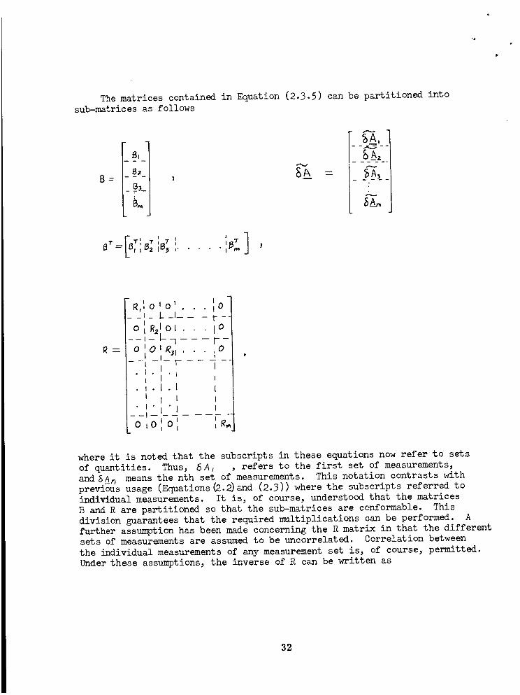
Thematrices contained in Equation (2.3.5) can be partitioned intosub-matrices as follows
B
6!
B_
_ B3_
_A,
_'r= "r*, 7, 7 , I -rI i B2 IB._ ,..... )
_) --.
' i IR,,OIO . . i0
__l_ L_l__ - f--o Ii Rzl Ol . io__,- L_----_--
o 'O=R_I , ioI I
- II I _ I• " i
i I lI.I.I {
I I I I
" i'l'] I
IOI =
where it is noted that the subscripts in these equations now refer to sets
of quantities. Thus, 8 At , refers to the first set of measurements,
and _A_ means the nth set of measurements. This notation contrasts with
previous usage (Equations _.2)and (2.3)) where the subscripts referred to
individual measurements. It is, of course, understood that the matrices
B and R are partitioned so that the sub-matrices are conformable. This
division guarantees that the required multiplications can be performed. A
further assumption has been made concerning the R matrix in that the differentsets of measurements are assumed to be uncorrelated. Correlation between
the individual measurements of any measurement set is, of course, permitted.
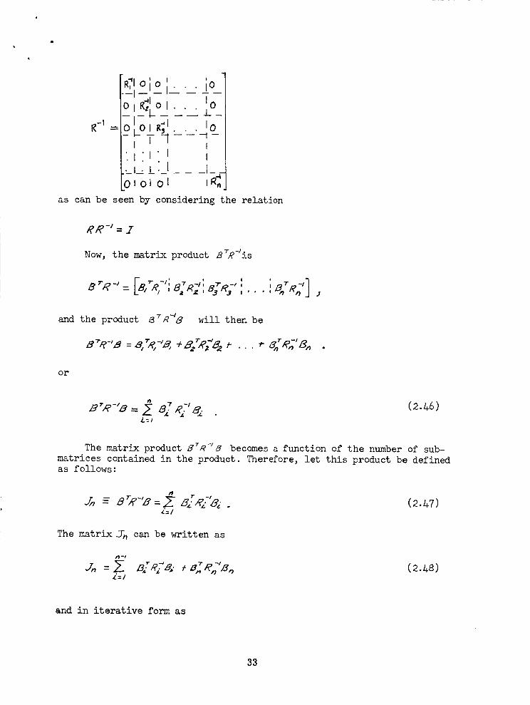
Under these assumptions, the inverse of R can be written as
32
[R2 313'. io
Jo: o ,o_ __.__ _L_
R-l = 010 1R_ j . I0
/:, :tl ,
Lo' o, o' ,_'.'as can be seen by considering the relation
RR -_= Z
Now, the matrix product gTR-Jis
B rR-' ,- -l; r_#_i, , ', , _" -i
and the product z37A'-i8 will then be
or
-/
L:I
The matrix product 8TR-/5 becomes a function of the number of sub-
matrices contained in the product. Therefore, let this product be definedas follows:
The matrix 2Tm can be written as
Z=/
and in iterative form as
33
Similarly, the matrix 8"rR-_A can be written as
(2._9)
_ 4R,_a,, _ ... -'__ (2..50)
Now defining
-- -- ,_=1 --
the iterative form of _ will be,
Equations (2.A5), (2.&9), and (2.51) can be used to express the estimateof the state vector that is obtained by processing all of the data up to
and including the nt_h set as follows:
(n) -i_Xo =_% ,
(2..53)
and the estimate obtained from processing all data up to and including the
(n-l) set is
_"'"_=_ ..Z"__,__',',-/(2.5z,)
The superscripts have been added to &x_o to indicate the quantity ofmeasurement data used in making the estimate. But, substitution of Equations
(2.L9) and (2.52) into Equation (2.53) yields the estimate of 8X o as
s'_°_ (4-, ,,_,_,_;,'%)-'(__,,_,,_, x,-'_q,,)__ --" -- _'',_ --
(2.55)
from which
34
I
(2.56)
But, from Equation (2.5/,),
(2.57)
Thus, Equation (2.56) can be written as
(2.53)
which reduces to
(s._,,a.r,s;,'g.)s__i"_--(_., ._.,TB.) s_T -'_(2.59)
Finally, multiplying both sides of Equation (2.59) by the inverse of (_o_/+"7" --/
_/_ 0 Bn ) y_elds
where from Equation (2._9)
_ (2.61)
Equations (2.60) and (2.61) are the iterative equations that are required
to compute the minimumvariance estimate.
In a similar manner, the recursive form of the covariance matrix for
the estimation errors can be developed. Consider the non-recursive form
s = C_-'_ _
35
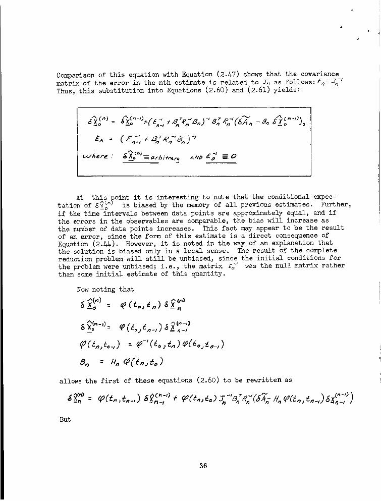
Comparisonof this equation with Equation (2._7) showsthat the covariancematrix of the error in the nth estimate is related to _ as follows: #_--_-JThus, this substitution into Equations (2.60) and (2.61) yields:
,5_Xo =
_,_ =
. o =_rb;fr4r_ AIVD £o ! _---0
At this point it is interesting to ncg e that the conditional expec-
tation of __co_) is biased by the memory of all previous estimates. Further,
if the time intervals between data points are approximately equal, and if
the errors in the observables are comparable, the bias will increase as
the number of data points increases. This fact may appear to be the result
of an error, since the form of this estimate is a direct consequence of
Equation (2._&). However, it is noted in the way of an explanation that
the solution is biased only in a local sense. The result of the complete
reduction problem will still be unbiased, since the initial conditions for
the problem were unbiased; i.e., the matrix ES was the null matrix rather
than some initial estimate of this quantity.
Now noting that
allows the first of these equations (2.60) to be rewritten as
But
36
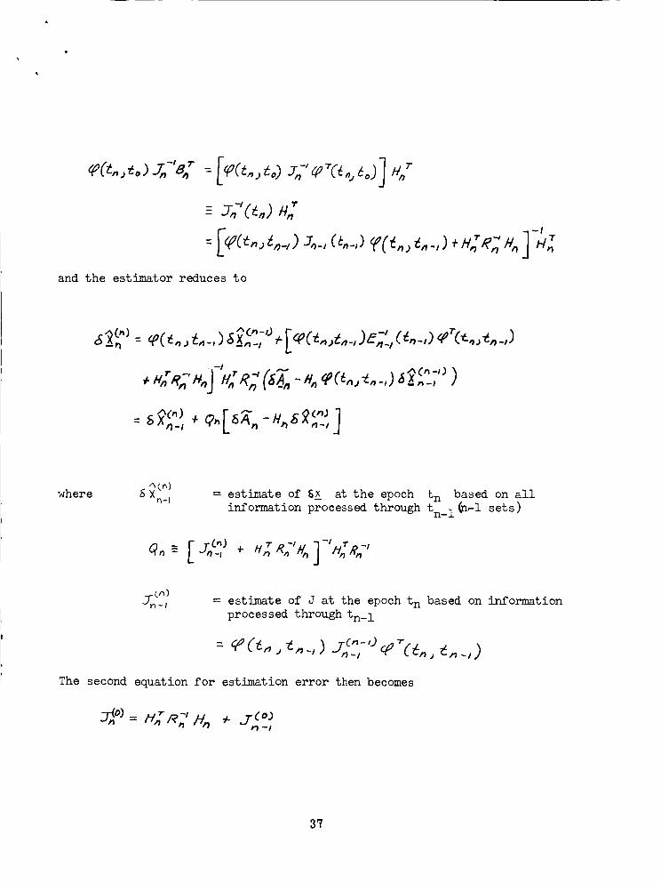
q
: _-_C_._Iv,,"
and the estimator reduces to
•- .!>.Cn-O I -I
+H_e,, H,_],,,, "'n -
[ _c,,, J= $"n-/
where E _ C'_)= estimate of 6X_ at the epoch tn based on all
information processed through tn_ 1 _l sets)
qo-[ _._°_o_,+.__:'_,o]-'<_-,
j-nC_)-I = estimate of J at the epoch tn based on information
processed through tn_ 1
The second equation for estimation error then becomes
= /-//_R_ H,_ * ,_-,
37
or
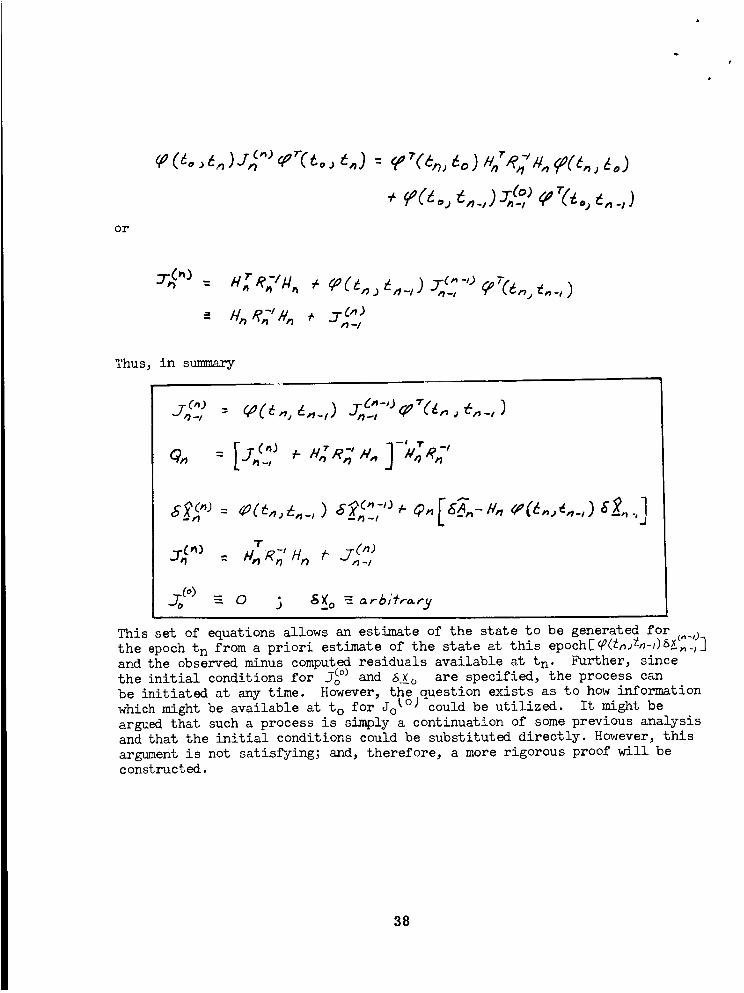
Thus, in summary
- [J_"_ " -' ] g,,R,,-'" -'(_" t "-' ,,-H,_R,,,V,,
T
./f') =- 0 5 ___o - a,-biY',-o, ry
This set of equations allows an estimate of the state to be generated forthe epoch tn from a priori estimate of the state at this epoch[_(_Zn-/)S_-_--'_]
and the observed minus computed residuals available at tn. Further, since
the initial conditions for _o(_ and 6X o are specified, the process can
be initiated at any time. However, the question exists as to how information
which might be available at to for Jo [°) could be utilized. It might be
argued that such a process is simply a continuation of some previous analysisand that the initial conditions could be substituted directly. However, this
argument is not satisfying; and, therefore, a more rigorous proof will be
constructed.
38
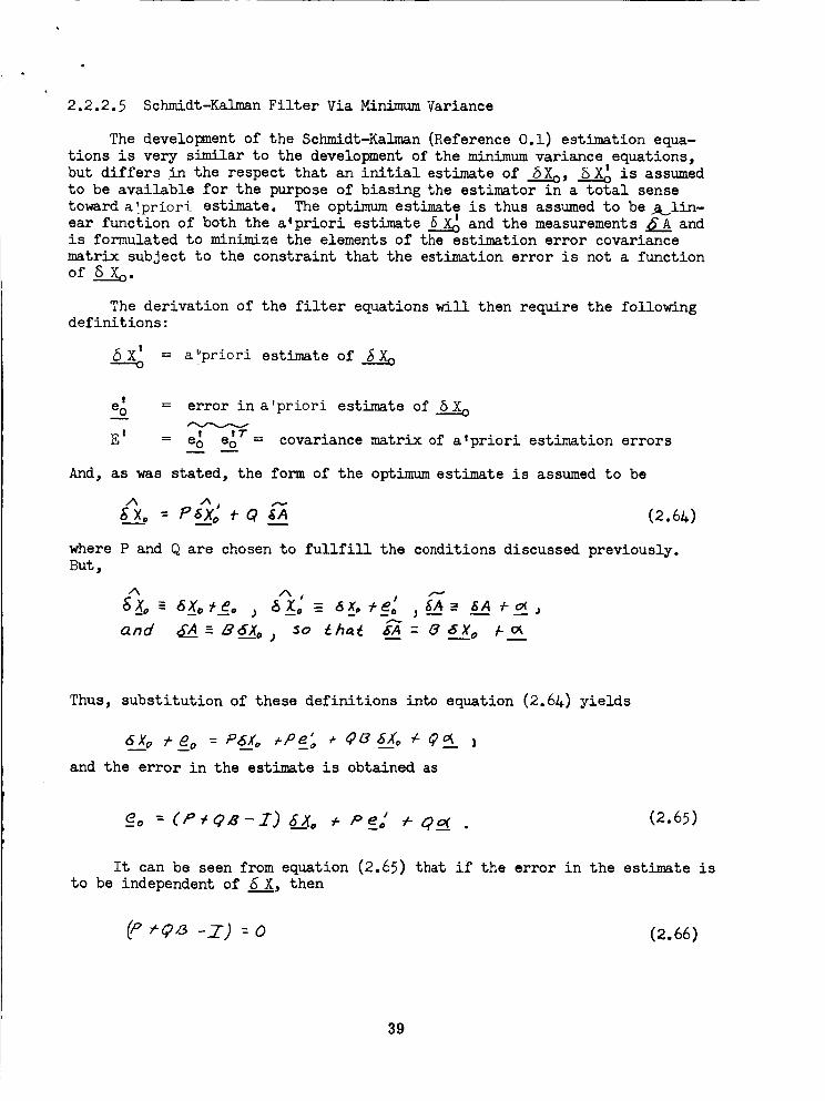
2.2.2.5 Schmidt-Kalman Filter Via MinimumVariance
The development of the Schmidt-Kalman (Reference O.1) estimation equa-
tions is very similar to the development of the minimum variance equations,
but differs in the respect that an initial estimate of ___XoX,_ is assumedto be available for the purpose of biasing the estimator in a total sense
toward a!priori estimate. The optimum estimate is thus assumed to be_klin-
ear function of both the aqpriori estimate _ and the measurements _A andis formulated to minimize the elements of the estimation error covariance
matrix subject to the constraint that the estimation error is not a function
of S___Xoo
The derivation of the filter equations will then require the followingdefinitions:
____X' = aV'priori estimate of____o
e_ = error in atpriori estimate of 8_oX
iTE' = e_ e o = covariance matrix of a'priori estimation errors
And, as was stated, the form of the optimum estimate is assumed to be
X___= P,5__.Xo .I-Q ,SA (2.6/+)
where P and Q are chosen to fullfill the conditions discussed previously.
But,
/_ ' ' _A- = _A /-o( agX0 6x0 eo _z0=_6x0t_e0 _ _
Thus, substitution of these definitions into equation (2.6&) yields
and the error in the estimate is obtained as
It can be seen from equation (2.65) that if the error in the estimate is
to be independent of g__XX,then
-Z) = o (2.66)
39
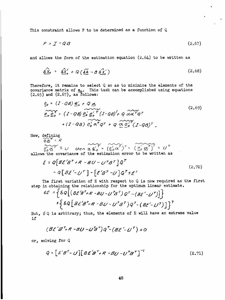
This constraint allows P to be determined as a function of Q
P =i-@8 (2.67)
and allows the form of the estimation equation (2.6_) to be written as
(2.68)
Therefore, it remains to select Q so as to minimize the elements of the
covariance matrix of e^. This task can be accomplished using equations
(2.65) and (2.67), as-_ollows:
eo (z-4)B)_o, Q__
+cz-Qa) eo _TQT , e __e_o(z__8)_.
(2.69)
Now, defining
eo%_ =-u _ _'J= (__S_)_ (___)_ u _allows the covariance of the estimation error to be written as
E=_[se'8",.-eu-u_,]o_(_.7o)
- _[_'-u _] - [E'8_-_]_ _E'The first variation of E with respect to Q is now required as the first
step in obtaining the relationship for the optimum linear estimate.
+{ ,sO[nE'e_e -su- u'e")<p'-(ee'-u")] 7"But, 5 Q is arbitrary; thus, the elements of E will have an extreme value
if
or, solving for Q
4>: [_'s"- u][_E_'_e -Bu-u__"] -' (2.71)
40
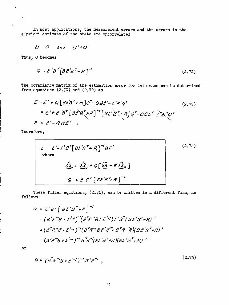
In most applications, the measurementerrors and the errors in thea'priori estimate of the state are uncorrelated
U = 0 ond
Thus, Q becomes
U_=O
Q =E'8"Fs_'8",R3-' (2.72)
The covariance matrix of the estimation error for this case can be determined
from equations (2.70) and (2.72) as
(2.73)
Therefore,
(2.74):_'--E'B'[BL:'B_'+RJ-'_E'where
_p : _'B>-[_-'B_,,-R]-'
These filter equations, (2.7L), can be written in a different form, asfollows :
_-(s_,_-,8__'-,)-'(B_-'__e'-,)_'B_(_E'_,R)-'
-_(BTR-_B ÷ E/-/)-/(BTR-'SE'B_'/. Br_'-_,)(/3E'BT÷RJ -'
(2.75)
or
41
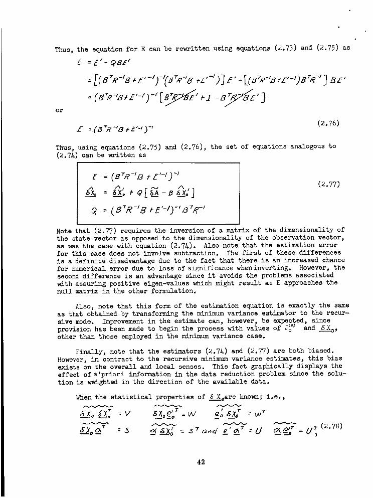
Thus, the equation for E can be rewritten using equations (2.73) and (2.75) as
E :E/-Qz_E"
or
f --(s "R -'a ÷_"".)-'(2.76)
Thus, using equations (2.75) and (2.76), the set of equations analogous to
(2.7&) can be written as
z = E'-/) -'/%1 /_/
q = (STR'8 ÷ -I
(2.77)
Note that (2.77) requires the inversion of a matrix of the dimensionality of
the state vector as opposed to the dimensionality of the observation vector,
as was the case with equation (2.7&). Also note that the estimation errorfor this case does not involve subtraction. The first of these differences
is a definite disadvantage due to the fact that there is an increased chance
for numerical error due to loss of significance wheuinverting. However, the
second difference is an advantage since it avoids the problems associated
with assuring positive eigen-values which might result as E approaches thenull matrix in the other formulation.
Also, note that this form of the estimation equation is exactly the same
as that obtained by transforming the minimum variance estimator to the recur-
sive mode. Improvement in the estimate can, however, be expected, sinceprovision has been made to begin the process with values of J_) and___XoX,
other than those employed in the minimumvariance case.
Finally, note that the estimators (2.%) and (2.77) are both biased.
However, in contract to the recursive minimum variance estimates, this biasexists on the overall and local senses. This fact graphically displays the
effect of a'priori information in the data reduction problem since the solu-
tion is weighted in the direction of the available data.
When the statistical properties of 8___Xoare known; i.e.,
_ _ _z r (2.78)£__Xoo_T_ = S o_X r_o = _Ta_d a'o_ 7 =U o___o =U,
42
this additional information can be used to improve the estimate of S___Xo. The
equations required to utilize this information can be obtained by simply
removing the constraint equation (2.66). _en this step is performed, the
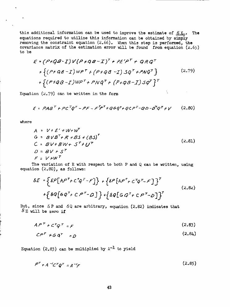
covariance matrix of the estimation error will be found from equation (2.65)to be
E.(P,'@B-Z)V(,o,Oa-Z)' + :E'/" :-ORO _
+[ :'+o8-zJwP'+:NO',
Equation (2.79) can be written in the form
(2.79)
E = pASry'pcT@T-PF-,:rpr+@6"@7+@dPZ-@D-D_qr÷v ' (2.80)
where
A = V+E'+W+w T
C = 8V+BW_- ST+LI T
O = 8V_-..S "T
F : V/-W x
The variation of _, with respect to both P and Q can be written, usingequation (2.80), as follows:
(_.81)
But, since 6 P and _Q are arbitrary, equation (2.82) indicates thatSE will be zero if
(_.8_)
(2.83)
(2.84)
Equation (2.83) can be multiplied by A-1 to yield
pT _-A -:Cr@ _-= A -"F (2.85)
43
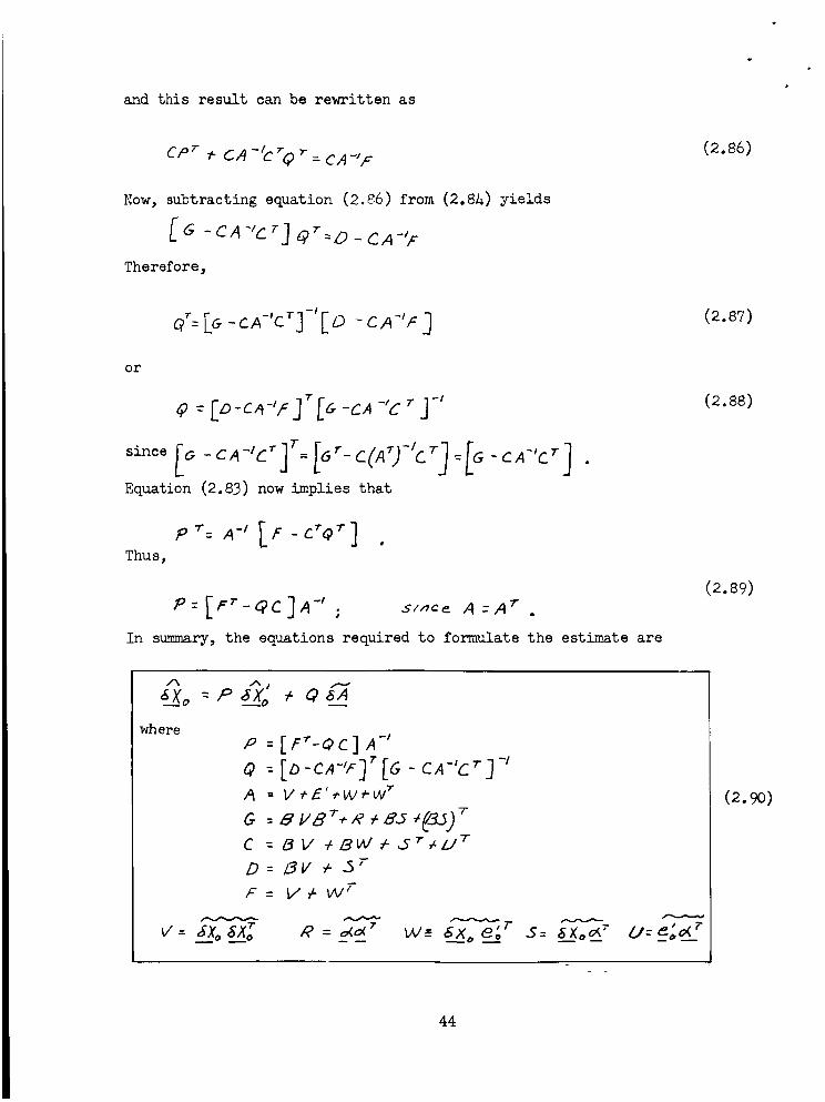
and this result can be rewritten as
CPr * CA -/c _Q _ = CA-'F
Now, subtracting equation (2.86) from (2.8A) yields
[ _ -c_"c,] Q'_D -cA-'rTherefore,
(2.86)
_':E_-_A-'c']-'[o-cA-'F] (2.87)
or
- [_-_-'r 3"[_ -cA-'c_J-'
Equation (2,83) now _,plies that
P "= A-' [F -C'Q'] •
Thus,
,: [,'-oc]A-' ; .s,'.,_c _ A = A T
In summary, the equations required to formulate the estimate are
(2.B8)
(2.s9)
A J%l
where--!
p :[r'-Qc]AQ :[_-cA-',,]"[G-cA-'c_3-'A = V*£'_'W_'W _"
C - SV ÷SV_,Sr,_U w
D: /3V ÷ -5"
F= V_-VV F
R = _<_x_ W.- 6X_ e ;r S= 6Xo_'
(2._)
44
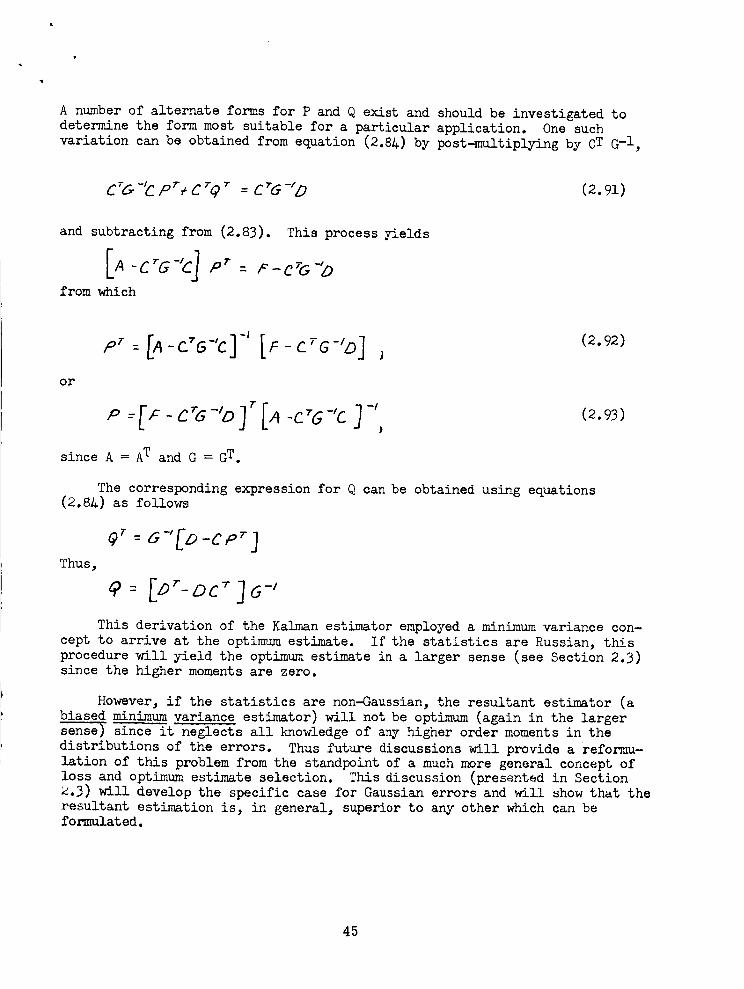
A number of alternate forms for P and Q exist and should be investigated to
determine the form most suitable for a particular application. One such
variation can be obtained from equation (2.8&) by post-multiplying by cT G-l,
p,,, T = c 'G-,o (2.91)
and subtracting from (2.83). This process yields
IA_CTG-_CJ pr _ F_Cz G_,D
from which
(2.92)
or
since A = AT and G = GT.
(2.93)
The corresponding expression for Q can be obtained using equations(2.8A) as follows
Thus,
This derivation of the Kalman estimator employed a minimum variance con-
cept to arrive at the optimum estimate. If the statistics are Russian, this
procedure will yield the optimum estimate in a larger sense (see Section 2.3)
since the higher moments are zero.
However, if the statistics are non-Gaussian, the resultant estimator (a
biased minimum variance estimator) will not be optimum (again in the largersense_ since it neglects all knowledge of any higher order moments in the
distributions of the errors. Thus future discussions will provide a reformu-
lation of this problem from the standpoint of a much more general concept of
loss and optimum estimate selection. This discussion (presented in Section
2.3) will develop the specific case for Gaussian errors and _<lll show that the
resultant estimation is, in general, superior to any other which can beformulated.
45
2.3 STATISTICALESTIMATIONTHEORY
2.3 •i Introduction
The discussions presented in section 2.2 lead to the simple development
of a series of computational algorithms which defined an estimabe of the statedeviation vector in terms of a series of observations and the initial condi-
tions. However, implicit in this material were the assumptions that
l) the dynamical model was linear
2) the observation model was linear
3) the optimum estimate of the state deviation was a linear function
of the observed minus computed values of the observables
A) only second-order statistics were necessary.
Further, the "loss" functions employed to develop optimum estimates of
the state deviation vector, while similar, were intuitive, thus giving rise
to questions regarding the uniqueness of the estimates generated. For these
reasons, it is now desirable to re-examine the estimation problem to demon-
strate the manner in which these assumptions can be relaxed and to show that
all of these estimators are special cases of a more general family of estima-
tors. Specific attention will be focused on:
l) the criteria to be utilized in determining the optimality of theestimate
2) the statistical properties of the variables, and
3) the form of the function relating the observables and the quantities
being estimated.
In general, the particular problems of interest are representative of a class
of problems which is the subject of the general theory of parameters estimation
as set forth in statistical decision theory. Therefore, the fundamental con-
cepts of the theory of parameter estimation form a basis for an adequatelyunified approach to fulfill the present requirements. It should be noted that
the simple derivation of filtering methods employs some of the basic concepts
of the theory of parameter estimation explicitly, while others are almost
always implicitly involved. However, when these concepts are not consistently
employed on an explicit basis, their applicability and usefulness are not
fully realized or exploited. In the subsequent sections on estimation, the
basic concepts of the general theory of parameter estimation are presented
for the primary purpose of formulating a more unified approach to determining
filtering methods than the simple approaches outlined previously. The dis-
cussions do not present an exhaustive treatment of the subject, nor is one
intended; rather, primary emphasis is placed upon the basic concepts which
46
have general applicability and particular usefulness to the present problems.Nonetheless, adequately complete discussions of the concepts are presented sothat extensions can be formulated and applied to those problemswhich requirethem.
It should be emphasizedat the outset that the problem of state estima-tion in space navigation and guidanceis completely equivalent to the problemof transmission and reception of information in a noisy communicationchannel.All of the methodsutilized for solving the latter problem are totally anddirectly applicable to the former one. Further, since extensive applicationof the general theory of parameter estimation has beenmadeto the generalproblem of communicationsin the presenceof noise, leading to a generaltheory of statistical communications,the sameapproach to state estimationwill yield a general theory of statistical navigation and guidance, Shouldquestions arise during the discussions, it is likely that answerscan befound in Referencessuch as 0.4.
In the discussions, it is assumedthat the reader is generally familiarwith the fundamentals of probability theory. To be specific, knowledgeisassumedof: (1) continuous joint probability distribution and density func-tions; (2) marginal and conditional probability density functions; and (3)conditional expectations. Thoughan extensive knowledgeof statistics is notrequired. This level of familiarity must be assumedsince to do otherwisewould require the developmentof all of the statistical concepts to beemployed. Thus, should the terminology be unfamiliar, the reader is referredto any of a numberof excellent references (References0.4, 3.1, 3.2, etc.).
The discussions begin (section 2.3.2) with basic notation and definitions,which are of particular concern to the present subject, and which are notnecessarily emphasizedin the fundamentals of probability theory. Thismaterial is followed (section 2.3.3) with a description of the basic problemto be considered in mathematical form and a discussion of somephysical inter-pretations.
In section 2.3.4, the rudiments of parameterestimation are discussed,and a basic description of the problem is given which emphasizesthe under-lying concepts. Thesediscussions define estimators, estimation error andbasic properties of estimators. Properties of a "good" estimator are thendiscussed to form a basic concept of estimation. Next, moregeneral criteriafor estimation are defined in terms of loss functions and associated risk.Properties of estimators which are basedon estimator risk follow these dis-cussions. Finally, sufficiency of an estimator is discussed, a sufficientstatistic is defined, and a test for sufficient statistics is given.
The determination of particular estimators is discussed in section _.3.5with primary attention given to useful methodsfor determining estimators.The determination of minimumvariance unbiasedestimators by meansof suffi-cient statistics and complete probability density functions is discussed, andthe methodof least-squares estimation is shownto yield minimumvariance esti-mators under the condition of statisticsl independenceof the sample. Attentionthen turns to the developmentof a lower boundfor estimator variance and thedetermination of Bayesestimators. Th___egeneralsolution (in terms of the
47
Bayesestimator) for the case of squared error loss is Shownto be the con-ditional expectation. (Moregeneral loss functions are also considered.)Following this material, Bayesrisk is discussed and a comparisonof a Bayesestimator and a minimumvariance estimator is given to illustrate the differsence in the results. Finally, minimumrisk estimation is discussed toemphasizethe use of sufficient statistics in minimizing risk for the generalclass of convexloss functions. (Maximumlikelihood estimation is discussedand shownto be equivalent to Bayesestimationwith a simple loss function.)
Thesediscussions conclude (section 2.3.6) with the application of Bayesestimation to the caseof manydegrees of freedom. The first result is theformulation of the technique to develop the optimumestimator for the generalvector case and for general statistical distributions. The secondresult isthe extension of this material to the general linear case, wherethe statis-tics are Gaussian. This extension develops a proof that (under these assump-tions) the Kalmanestimator is th___eeoptimumestimator.This fact could notbe developedfrom the material presented in section 2.2.
2.3.2 Basic Definitions
It is the purpose of the following sections to develop a basic under-
standing of the general problem of parameter estimation. This effort must
necessarily begin with the following basic definitions of the essential
elements of the problem.
2.3.2.1 Random Processes
A random process is defined herein as any phenomenon for which repeated
observations, under a given set of conditions, do not yield identical results.
In general, random processes are characterized by variations in outcomes for
repeated equivalent trails. These variations in outcomes or observations areconsidered as the,randomness" of the process, which is equivalent to uncertain-
ty in the outcome of the process. As a contrary example, consider a process
whose behavior is completely described by a known system of differential
equations. Theoretically, it is possible to completely determine the
behavior of such a process if a sufficient finite set of initial conditions
are known. Thus, it would be possible to completely specify the future
behavior of such a process if an adequate set of observations are made at
some time. Such a process is said to possess deterministic regularity. How-
ever, until such time that all physical laws are explicitly established for
the microscopic and infinitesimal domains, the concept of random physical
processes must be admitted, accepted, and dealt with.
Alternatively, a random process could be defined as one which does not
possess deterministic regularity, and subsequent outcomes cannot be predicted
with certainty from a set of observations of the process. However, a random
process can possess definite properties of behavior which make possible adescription on a statistical basis. Such random processes are said to
possess statistical regularity. In such cases, even though particular out-
comes of the process cannot be specified, it is possible to specify the rela-
tive frequency or probability of occurrence of outcomes for the process. That
is, let y denote the outcome of a random process, then the process is
48
described by specifying the probability that y _ill lie in somearbitraryinterval. The commonnotation is as follows:
In this notation P(a _ y _ b) is referred to as the probability distributionfunction which is the probability that y lies in the interval a < _ b, andf(y) is the probability density function of y.
Thus, randomprocesses are explicitly described by specifying theirprobability density functions. In Section 2.3.3 a detailed mathematicaldescription is given for randomprocesses of particular interest in the pres-ent discussions.
For the sakeof notational convenience, "pdf" will be used to denote"probability density function" in the text, and "f(y)" will denote the pdf ofy in equations. However,it should be noted that if x and y are two differ-ent randomprocessesthe pdf of x, f(x), is not equal to the pdf of y, f(y),even for y = x.
2.3.2.2 Parameters
If a randomprocess possessesstatistical regularity, then it can bedescribed by specifying all of its statistical properties, which is equivalentto specifying the pdf of the process. The "parameters" of a randomprocessare defined as the smallest set of elementswhich specify the statisticalproperties of the process or its pdf. In general, all statistical averages,or moments, of a randomprocess are required to specify it. However, formanyprocesses of interest, all momentsare not required, and a smaller setof parameters suffices to specify the process.
For example, in the case of a Gaussiandistributed randomprocess, it isonly necessary to specify the meanand variance of the process, since the pdfof the process, f(y), is specified by these two parameters; i.e., if y is theoutcomeof a Gaussiandistributed randomprocess, then
where _ and _2 (the meanand variance of y, respectively) represent the twoparameterswhich specify the pdf of a Gaussianrandomprocess.
In general, the set of n parameterswhich specifies the statistical proper-
ties of the pdf of a random process will be denoted by @ = (@l, @2' "'', @snt)"The pdf of a random process will be shown as a function of the parameter@ in terms of the conditional pdf, given 9; i.e., f(yZ@). For the Gaussian
ixif Q= = 0"-2) and = f(J ,
49
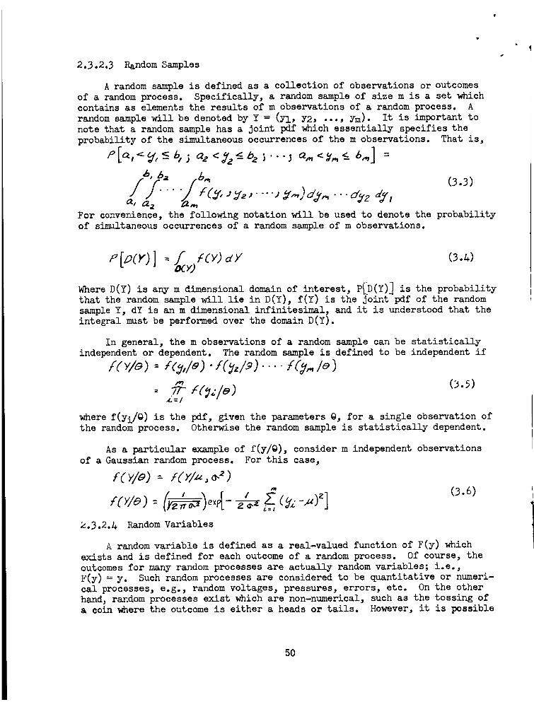
2.3.2.3 Random Samples
A ra_om sample is defined as a collection of observ_ions or outcomes
of a random process. Specifically, a random sample of size m is a set which
contains as eleme_s the results of m observations of a random process. A
random sample will be denoted by Y = (_, _, ..., Ym). It is important to
note that a random sample has a joint pdf which essential_ specifies the
prob_i_ty of the simultaneous occurrences of the m observations. That is,
L (3.3)For conve_ence, the follo_ng notation wi_ be used to denote the prob_ility
of s_taneous occ_rences of a r_dom sample of m observations.
Where D(Y) is any m dimensional domain of interest, P_D(Y)_ is the probability
that the random sample will lie in D(Y), f(Y) is the Joint pdf of the random
sample Y, dY is an m dimensional infinitesimal, and it is understood that the
integral must be performed over the domain D(Y).
In general, the m observations of a random sample can be statistically
independent or dependent. The random sample is defined to be independent if
f( ) : . .... le ),,, )
X:= l
where f(yi/@) is the pdf, given the parameters 9, for a single observation of
the random process. Otherwise the random sample is statistically dependent.
As a particular example of f(y/@), consider m independent observations
of a Gaussian random process. For this case,
2.3.2._ Random Variables
A random variable is defined as a real-valued function of F(y) which
exists and is defined for each outcome of a random process. Of course, the
outcomes for many random processes are actually random variables; i.e.,
F(y) = y. Such random processes are considered to be quantitative or numeri-
cal processes, e.g., random voltages, pressures, errors, etc. On the other
hand, random processes exist which are non-numerical, such as the tossing ofa coin where the outcome is either a heads or tails. However, it is possible
5O
to define a randomvariable for this randomprocess by assigning numberstothe outcomesor by defining the randomvariable to the numberof headsin mtosses of a coin, etc.
The importance of the concept of a random variable lies in the fact that
many of the arithmetic, algebraic and analytical operations which are defined
for real-valued functions are meaningful for random variables, whereas they
are not for the outcomes of all random processes. Thus, additions, subtrac-
tions, multiplications, transformations, etc., are applicable to randomvariables.
In general, if y possesses statistical regularity, then the random vari-
able F(y) possesses statistical regularity. Thus, F(y) is generally specified
by a pdf which is derived from that of y. The derivation of f IF(y)_ from
f(y) is, in general, not a simple transformation, except in the simple case
of F(y) = ay for which f [F(y)_= a • f(y), where a is a constant. However,
the expected values of random variables are usually required, and the pdf of
F(y) is not required since the expected value of any random variable F(y) can
be determined from pdf of y as follows:
where E denotes "expected value." The conditional expectation of F(y),
@, is defined as
given
2.3.2.5 Statistic
A statistic is a known function of a random sample of observations of a
random process whose outcomes are random variables. It follows that a sta-
tistic is a random variable; however, a random variable is not necessarily a
statistic. For example, in the case of a Gaussian random variable y with
unknown mean value _, the function y -_ is a random variable; however, it
is not a statistic since_is not known. On the other hand, y - c, where c
is a known constant, is a statistic.
The important difference is that a statistic is defined as a known func-
tion of a random variable sample set Y which does not contain any unknown
elements. Thus, a particular sample Y specifies the statistic. Of course,
statistics are not unique since many known functions of a random variable
sample can be defined. In general, the set of statistics defined for the
random variable sample set Y will be denoted by
T(Y) =[TI(Y), T2(Y), T3(Y) .... ] •
A statistic represents a transformation of the sample set Y from the
space of random variable observations to the space of statistics. The trans-
formation is not unique for a given statistic. For example, a statistic can
be the simple linear sum of random variable observations in which case many
51
different samplesets transform into the samepoint in the statistic space(i.e., various samplesets can yield the samenumerical value of the statistic ).
Theconditional expectation of T(Y), given 9, is determined from theconditional Joint pdf of Y, i.e..
Ywhere the integral is m dimensional and must be performed over all y in Y.
2.3.2.6 Complete Probability Density Functions
In the consideration of parameter estimation, a question often arises
concerning the uniqueness of the expectation of a random variable. This
question can be resolved in terms of the property of completeness of pdf's.A random process, y, is specified by its pdf, f(y/@), which is a function of
@. For any interval of @, A _ @ _ B, f(y/@) defines a family of pdf's. The
following definition defines a complete family of pdf's.
DEFINITION: let f(y/@) _ 0 for any interval of a ( y • b and zero
otherwise and let F(y) be a random variable defined on the interval a _ y < b
and independent of @.
Now, if
if, and only if, F(y) _ 0 for a _y • b, then f(y/@) is defined to be a com-
plete family of pdf's. Conversely, if there exists some F(y) which is not
identically zero in a _ y <b for which E _F(y)_ =0 for all A _ @ < B, then
f(y/@) is not a complete family of pdf's.
It should be noted that a pdf can be complete with respect to certain
parameters. For example, consider the Gaussian pdf, f(y/_ , _2), to wit,
If the mean value_ is known, then any random variable F(y) which is defined
as an odd function about_ has zero expected value and, hence, f(y/_, 0 2) is
not complete with respect to _2 for known_. On the other hand, if_ is
unknown, then f(y/zx, _2) is complete with respect to both_ and _ 2 since
the only F(y) which has zero expected value for all_ and _2 is given byF(y) _ O. Of course, f(y/_,_) is complete for known o_2 if _ is unknown.
The use of completeness can be demonstrated by considering f(y/_,_2)
for _2 = 1. Let F(y) =y2; then E _F(y)] = E(_) = _2 + 1. The property
of completeness determines that there is no other F(y) _y_ such that
E_(y)_ = 2 + 1. For if E_F(y)_ = E(_), then E_F(y) - _] = O. But
since f(y/_, l) is complete, F(y) - y_ must be identically zero for all y;
i.e., F(y) _y_. Thus, since f(y/_, l) is complete, the E_F(y)Sis uniquely
determined.
52
2.3.3 A Mathematical Description of Random Processes
In order to promote an understanding of parameter estimation with respect
to the particular problems of interest, a mathematical description is discussed
in this section which describes, in general form, the set of random processesto be considered.
2.3.3.1 A General Form
For present purposes random processes will be defined in general form asfollows
= EC_e) e (3.7)
where
= m x 1 Observation vector
@ = n x 1 Parameter vectorm
F = m x i Transformation vector
e = m x 1 Noise vector
Equation (3.7) defines a random process as a general non-linear function of
the parameter vector @. The general linear case is defined by _(@) = A@;
i.e.,
= (3.8)
where
A = m x n Transformation matrix
The foregoing terms have the following properties.
e Is always random
@ Is either random or non-random
F Is always non-random
A Is always non-random
Is always random
Thus, for present purposes, a random process is defined as the linear sum
of two processes _(@) and _. The process _ is always a random process. How-
ever, since _ is always non-random, the process _(@) is randon if, and only
if, @ is random. It is extremely important to note that for non-random @,
the process _(@) possesses deterministic regularity. Furthermore, the process
_(@) possesses conditional deterministic regularity, given @; i.e., for a par-
ticular @, _(@) is deterministically regular. Of course, Z is always random
53
since e is always random.
A moredetailed discussion of the general form of randomprocesses isgiven in subsequentsections. However,at present it is advisable to discusssomephysical interpretations of the randomprocess as defined herein.
2.3.3._ SomePhysical Interpretations
In the general form of a randomprocess, the vector @represents theessential unknownswhich are to be determined. For example, in the linearcase, @ represents the "state" vector which is commonlyused to denote theposition and velocity deviations of a spacecraft from a reference trajectory.However,in the present definition @ is quite general and can represent otherparameters suchas the coefficients of a polynomial fit to data (as in thecase of least-squares curve fitting) or the bias arising from a randompro-cess, etc.
Thevector _(@) represents someobservable or measurablephysicalphenomenawhich is dependenton @. In general, _ represents a set of knownnon-randomfunctions of @. In the case where@represents spacecraft positionand velocity deviations from a reference trajectory, _(@) usually representsdeviations of spacemeasurementsfrom the reference. In this case, _(@)usually becomesA@whereA is the matrix of first partial derivatives of spacemeasurementswith respect to spacecraft position and velocity. It should benoted that, in general, _ is not necessarily constant; e.g., _ can vary as anon-randomfunction of time. For example, @can denote trajectory injectiondeviations which are propogatedinto subsequentvalues of trajectory devia-tions as a function of time. In such case, _(@) is a function of a time-dependenttransition matrix.
The vector _ represents errors in measurementsof _(@) or, equivalently,the uncertainty in observations. If the errors in measurementswere notpresent, then, theoretically, the parameters @could be determined directlyfrom the inverse of Z = _(_); i.e., for _ _ O, @= F--I(z) whereF-I existsand y is an adequate set. However,in the general case, _ is present andcannot be determined from F-1 without the risk of large errors in the results,e.g., in the linear case w_ereZ = A@+ _, A-_ = @+ A-1 e and the error intaking @= A-_ is A-1 _which could be large dependingon-the nature of A-1and _.
The vector _ is a randomvariable vector which represents the randomprocess in general. A particular value of Z represents a particular observa-tion of the randomprocess. The totality of observations comprises a randomsampleset Y which contains all observations of the randomprocess. The vector_and the set Y can be interpreted in two equivalent forms. In general, thetotality of observations can be taken in a time sequenceof simultaneousobservations of the elements of _. In this case, Y contains the set of par-ticular observations of Z, i.e., Y = (_l" Y%_,.... , _m)- However, the vector
can represent the totality of observations with the elements of Y as sub-vectors of _, in which caseY and _ are the sameset. The particular inter-pretation of _ is selected on the basis of convenience for a particularproblem.
9
54
2.3.3.3 An Ensembleof Non-StationaryRandomProcesses
In the general form of a randomprocess, as defined in equation (3.7),the termS(@) is dependenton @and can vary as a function of time. Thus, thegeneral form of randomprocesses actually defines an ensembleof non-station-ary randomprocesses. Eachparticular value of @defines a particular memberof the ensembleof randomprocesses defined. Since _(@) can vary with timefor any g, the ensemblemembersare non-stationary; however, if _(g) is inde-pendent of time, i.e., constant for all particular @, then each memberof theensembleis stationary, assumingthat the randomprocess _ is stationary.
Twoimportant aspects of the ensembleof randomprocesses should bestrongly emphasized: First, it is important to note that whena set of obser-vations are madeof a randomprocess, a particular memberof an ensembleisobservedand determining @is equivalent to determining which memberof theensemblehas been observed. That is, during a sequenceof observations,is a constant which, of course, is unknown. The object of making observationsis to determine @, if possible. It should be noted that for each ensemblemember,the deterministic regularity resulting from _(@) is reflected asstatistical regularity in the observations _ = _(@) + e.
Second, it is also important to note that although @is an unknownto bedetermined, certain information is often available concerning the behavior of@. Indeed, @is often a randomvariable with knownpdf. In such cases, itis possible to determine the probability of occurrence of particular membersof the ensemble. In general, membersof the ensembleoccur with variousprobabilities and certain memberscan occur with zero probability. If @is arandomvariable, then the ensembleof randomprocessesis specified by theJoint pdf of @. Generally, @exists over someparameter space,A-L, and thepdf of @determines the probability of occurrence of a particular @in theparameter space£L.
2.3._ Rudiments of Parameter Estimation
2.3._.1 A Basic Description of Parameter Estimation
The problem of parameter estimation can be described most succinctly in
the following manner:
l) A random process exists which is a function of or characterized by a
set of parameters.
2) The parameters are not explicitly known nor can they be directly
observed.
3) Knowledge of the parameters is required to perform some particulartask.
_) Observations of the random process can be made which yield a set of
sample data.
5) The set of sample data provides the only means for determining the
required parameters.
55
Theforegoing is equivalent to the methodof inductive inference, whichis referred to as statistical inference whenrandomprocesses are involved.That is, from a particular set of observations, conclusions are drawnwhichconcernsomegeneral aspects of the process under observation. The methodisdepicted in Figure 2.3.1. It is a basic theoremof formal logic that themethodof inductive inference is intrinsically uncertain. It is not possibleto makegeneralizations with certainty on the basis of a set of particularobservations. The situation is apparent whenrandomprocesses are involved.Nonetheless, useful inferences can be madeif the procedures involved arejudiciously formulated. This is the general concern of the theory of statis-tical inference and the particular concern of statistical decision theory.
In the general theory of statistical inference, the basic problemwhichis considered, is that of makinga decision under existing conditions ofuncertainty. Twotypes of uncertainty are recognized: randomnessand thelack of knowledgeconcerning the state of nature. It is required to makeadecision concerning the state of nature, and it is desirable to makethe"best decision possible" under the circumstances. In effect, the decision isan estimation of the state of nature; thus, if the state of nature is deter-minedby a set of parameters, the decision problemof the parameter estimation.
Theforegoing situation is completely equivalent to the problem of deter-mining the set of parameters@of the randomprocess _ = _(@) + _. Theuncertainty due to randomnessis equivalent to the errors in measurementsorobservations, denotedby _, and the uncertainty due to the unknownstate ofnature is equivalent to that of the unknownparameters g. Of course, "best
decision possible" is equivalent to "best parameter estimation possible."
Thus, the problem of parameter estimation becomes that of determining esti-
mations of @ from a set of observation data which are "best" with respect to
some applicable criteria. Some comments concerning the general philosophyare in order.
At the outset (before observations are taken) there exists uncertainty
about the parameters @. However, some knowledge of @ can exist a'priori since
the pdf of @ is frequently known; i.e., the probability of occurrence of a
particular @ can be known a'priori. Thus, in general, complete uncertainty
concerning @ does not exist at the outset. Nonetheless, in each particular
case, it is required to know @ with less uncertainty on greater certainty (as
contrasted with absolute certainty) than exists a'priori. The statistical
regularity of the process, which is characterized by the parameter @, is
present in the observations of the process; hence, the observations must con-
tain intrinsic information concerning the parameters @. Thus, the object of
parameter estimation becomes that of extracting information concerning @ fromthe observations thereby decreasing the a'posteriori (after observations)
uncertainty of @ or, equivalently, increasing the a'posteriori knowledge of @.
It is interesting to note that the problem is identically equivalent to the
problem of information transmission and reception in the presence of noise,
which is considered in the general theory of statistical communication. Indeed,
the problem is one of extracting information concerning @ from the observations
Z in the presence of measurement or observation error @.
56
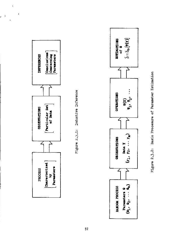
II I_l 1
;,4 w
L
o
ID
I.-I
o
I-I
_q
,4
.r--I
_o, _ ,
_°_
O
A
A
V
o
Ii)4o
o
o
.rt
;i
57
In general_ it is not possible to determine the parameters @ with abso-lute certainty (unless an infinite number of observations are made, which is
generally not practical) ; thus, some residual or a'posteriori uncertainty must
be expected. The concept of "best parameter estimation possible" is equival-
ent to the minimization of a'posteriori uncertainty or the extraction ofmaximum information from the observations.
In general, parameter estimations are derived from operations which are
performed on the set of observations or random sample data. These operations
are defined as estimators and are denoted herein by 6 . The general procedure
of parameter estimation is depicted in Figure 3.2. In the following section,estimators 8 are discussed in further detail.
2.3._.2 Estimator
In general, an estimator g is a known function of statistics (see Section
2.3.2.5) which provides an estimation of a parameter @. Of course, an estima-
tor is a random variable; in fact, estimators are a subclass of the class of
statistics. (That is, an estimator is a statistic but a statistic is not
necessarily an estimator.) In many cases the difference can be trivial; how-
ever, in the consideration of parameter estimation, it is extremely important
to consider all possible known functions of random samples, i.e., statistics.
The ambiguity can be resolved by considering a statistic as an admissible
estimator if its conditional expectation, given @, contains @ explicitly.
That is, if E(T/@) = @ + b(@), then the statistic T is an admissible estimator
6 for @, where b(@) is some function of @, which is referred to as estimator
"bias." It follows that
Thus, in general, admissible estimators can contain a "bias" term b(@) which
is a function of @. However, all admissible estimators are not necessarily
desirable since estimator bias, b(@), whereas admissible, is not necessarily
desirable in particular cases.
It should be noted that the term ,,estimator" denotes a function, whereas
"estimation" or "estimate" generally denotes a particular value of an esti-
mator as a function of a particular random sample.
There are two major objectives in the problem of parameter estimation.
The first of these objectives is to determine parameter estimators _ with
minimum uncertainty; and the second is to appraise the estimator's uncertainty
in terms of its magnitude and behavior as a function of significant factors;
e.g., sample size, random process characteristics, etc. Estimator uncertainty
is usually measured by estimator error, which is discussed below.
2.3._.3 Estimator Error
In general, parameter estimations are inductive inferences and as such
are always subject to uncertainty. The primary objective of parameter esti-
mation analyses is to determine estimators with minimum acceptable uncer-
tainty. In order to approach this problem on a mathematical basis, it is
necessary to express estimation uncertainty in explicit mathematical form.
58
Thus, with each estimator there is associated an estimator error, denoted by, which is defined as the linear difference of a parameters and its esti-
mation, to wit,
(3.9)
The problem of parameter estimation can be considered as equivalent to an
analysis of estimator error. Thus, at the outset, several general properties
of should be noted. First, estimator error is a function of the sample dataset and the parameter @; i.e.,
Second, since _ is a function of random variables, it is a random variable and
must be analyzed on a statistical basis, i.e., g is specified by determining
its pdf, f(_ ). Third, since _ is a function of Y and @, f(_ ) is a functionof f(Y) and f(@), to wit,
S_T(y)F°urth'_the particular form of f( a ) is dependent on the particular estimator
In the analysis of parameter estimators, primary emphasis is placed upon
the statistical behavior of estimator error. This behavior is dependent upon
the characteristics of the random process (especially as a function of the
parameters being estimated) and the particular form of the estimator as a
function of the sample data. The ultimate objective in parameter estimation
is to determine parameter estimators which yield acceptable behavior of the
estimator error. Of course, suitable statistical properties of estimator
error must be used as the object of analysis. The most significant properties
are the first moment, first central moment, and second moment, which are
usually referred to as the mean value, the variance and the mean squared valueof estimator error, respectively. These quantities are defined below:
(i) Mean value of g =
= E(e)
fCe) de
= E(6)- ECG
59
(2) Variance of _ = V(C )
VCC)=E(_- g)2
= l( ( _ _ )2 f(E ) d
(3) Mean-Squared Value of g = g_
= E(c _)
=/_C 2f(_) d_
The mean value of _ is commonly referred to as estimator bias and if
= O, then £ is considered unbiased. The most significant aspect of esti-
mation error is the effect of _ on V(C ) and g_. This effect is stated below.
If for all @, the conditional expectation of £ , given @, is zero, then
the mean-squared value of g is equal to V(-C ) and the estimator variance,
V( 8 ). This can be shown in the following manner _ denotes expectation with
respect to @ and 5-@ denotes the conditional expectation E(£/@_:
= Ee E (G/e)
-_ eThus, if E(E/@) = 0 for all @, then_ = 0 and_ =V(_ ). Thatg -_ : V(8) for
E(g/@) = 0 is shown below:
(_.12)
)
6O
The secondterm is the square of E(£/@) and is always positive, thus,
¢* _ V(6) 0.]-3)
with equality if E(£/@) = 0 for all 0. Therefore, the following is true:
If E(g/@) = 0 for all @, then_ = V(_ ) = V(& ).
It should be noted that E(£/@) = 0 for all @ is a sufficient condition for
gz = V(6 ) = V(_ ). In general, the condition is also necessary if the pdf
of @ is non-zero from all @. On the other hand, if pdf of @ is zero for some
interval of @, then E(g/@) can be non-zero for the same interval of @, and
_2 =V(g ) =V(6) . This is true because if f(@) = 0 for some interval of @,
then those @ in this interval occur with zero probability and contribute
not_hing to the exoectation with respect to @. It should also be noted that
if _ = O,_thenc _ =V(£); however, it does not follow thatg-2 =V(6),since for 6 =@ it is not required that E(£/@) = O.
2.3._._ Basic Properties of Good Estimators
The primary motivation for the concept of a "good" estimator is derived
from a consideration of the basic properties of estimator error discussed pre-
viously. Consider three different estimators gl' _ and 63 for a parameter
@. Let the estimator errors for the three estimators be denoted by _, g 2
and £ 3, respectively, and assume that they have the following propertles forall @.-
The pdf's of 61,
_(cz/o)= o
_,(_/_)= o
E(C3/e) = _3
v(cl) < v(_2) < v(¢3)
6 2 and 5 3 are depicted below in Figure 2.3.3.
61
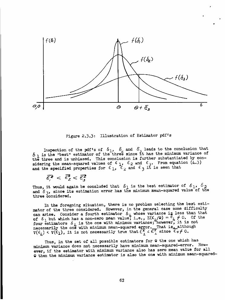
f s)
o e÷g
Figure 2.3.3: Illustration of Estimator pdfls
Inspection of the pdf's of ill, B_ and _ leads to the conclusion that
1 is the "best" estimator of the three since it has the minimum variance ofthe three and is unbiased. This conclusion is further substantiated by con-
sidering the mean-squared values of £ l, _2 and g3" From equation (4.3)
and the specified properties for £1, g2 and g3 i_ is seen that
Thus, it would again be concluded that S 1 is the best estimator of 51, 6 2
and 6 3, since its estimation error has the minimum mean-squared value of thethree bonsidered.
In the foregoing situation, there is no problem selecting the best esti-
mator of the three considered. However, in the general case some difficulty
can arise. Consider a fourth estimator _A whose variance i_ less than thatof gl but which has a non-zero mean value; i.e., E(gl./@ ) = eA _ 0. Of the
four estimators _ A is the one with minimum variance;_however_ it is notnecessarily the one with minimum mean-squared errror. That isA_although
z z _ since C_ O.V(E_) _ V(E1) , it is not necessarily true that _±
Thus, in the set of all possible estimators for @ the one which has
minimum variance does not necessarily have minimum mean-squared-error. How-
ever, if the estimator with minimumvariance also has zero mean value for all
@ then the minimum variance estimator is also the one with minimum mean-squared-
62
error in the subset. But, the minimumvariance estimator in this subset isnot necessarily _he minimummean-squared-errorestimator of the total set ofestimators.
It is apparent that, in general, somequestion exists concerning theselection of a "best" estimator. The final answer is usually dependentuponthe particular problembeing considered. Nonetheless, from the foregoingconsiderations someproperties of "good" estimators can be formulated whichactually classify or define sets of estimators as follows.
2.3._._.1 UnbiasedEstimators
An estimator is defined as an "unbiased" estimator of @if
= e :o,.
It follows that an unbiased estimator has zero mean-value of estimator error,
i.e.,
_.3.A._.2 Vh_uimum-Variance Estimators
An estimator is defined as a "minimum-variance" estimator of @ if it has
the smallest variance of all estimators of 9, for all @.
2.3.A._.3 Minimum-Variance Unbiased Estimators
An estimator is defined as a "minimum-variance unbiased" estimator if it
has the smallest variance of all unbiased estimators of @, for all @.
_.3.&.A.A Minimum Mean-Squared-Error Estimators
An estimator is defined as a ,.minimummean-squared-error" estimator of @
if it has the smallest mean-squared estimator error of all estimators of @,for all @.
2.3.&.5 Loss Functions and Risk
In the previous section, basic criteria for good estimators were based
upon estimator bias and variance, and mean-squared value of estimator error.
Although these criteria are generally acceptable, there always exists the
problem of selection between a minimum-variance and a minimummean-squared
error estimator when they are different. Furthermore, these criteria lack
generality in terms of total performance or behavior of an estimator. A more
general form of estimator performance criteria is formulated from the follow-
ing considerations.
In the general situation of parameter estimation, there exists more pen-
ality or "loss" which is associated with mu incorrect estimation. If this was
not true, then nothing essential could be gained by the efforts of determining
and using good estimators. The loss can be measured in terms of a non-negative
function of estimator error which is a monotonically increasing function of
83
estimator error magnitude. Any function of estimator error with these twofundamentalproperties is referred to as a loss function which will be denotedbyL(-C). Thus, a class of loss function is defined by
L(£ ) = 0 for g = O
2) : L(%_)for
L(E 2) >L(£ I) for I_I_ Ell
L(g- ) = L(- 6)
It is not necessary to restrict loss functions to the class with these
properties, although the class has general applicability. A class of loss
functions can be defined more generally as non-negative, monotonically non-
decreasing with a unique coincident minimum with estimator error magnitude.Such loss functions allow a cost of measurement to be included and are mini-
mum, rather than zero, for _ = O. Also, constant loss is allowed for an
interval of estimation error C .
Of course, negative loss would be considered as a gain; however, this isnot allowed for non-zero estimator error and for zero error the loss is sim-
ply zero or some minimum. Obviously, there are no unique loss functions of
estimator error; thus, a particular loss function should be selected on the
basis of a particular problem. IB should be noted that "squared-error" is anacceptable loss function, i.e., g = L((). Others can be as easily defined.
The loss function L(E) measures the loss incurred in making an error g
in an estimation of @ where it is assumed that some appropriate L(£) can be
defined for each problem of interest. Of course, L( g ) is a random variable
dependent on estimator error g = 8- @. Thus, L(£ ) = L(g, @) is a function
of _ and g and measures the loss incurred in estimating @ with 8 . The aver-
age value of L(8, @) is the loss to be expected in using the estimator _ for
@. Expected loss is generally referred to as the "risk" taken, i.e., the
risk is expected to be lost on the average. The risk in estimating @ by 6 is
function of both @ and 8 and will be denoted by R(_, g). It follows that
R(_,8) ---/"Z [,_(Y), o] f(Y/e} dyY
Risk or average loss provides a rather general criterion of estimator
performance. Of course, risk is always _ function of the particular lossfunction, which includes squared-error _; therefore, risk includes mean-
squared error _ as a particular case. In general, it is desirable to mini-
mize the risk involved in estimating @ by 6 . Thus, for a particular loss
L(6, @) it is desirable to select an estimator 6 which minimizes the expected
loss or risk in estimating @. This leads to a class of estimators referredto as minimum risk estimators which are defined as follows.
2.3.&.5.1 Minimum Risk Estimators
An estimator is defined as a "minimum risk" estimator for the loss func-
tion L(6, @) if the expected loss or risk R(_, @) is a minimum for all @.
64
There is no argumentconcerning the desirability of minimum risk esti-
mators; however, difficulty frequently arises in finding such estimators.
It is usually possible to find an estimator which has minimum risk for certain
@ but which does not have minimum risk for other @. A single minimum riskestimator does not exist. Such situations are untenable since @ is unknown
beforehand. Thus, two alternate approaches are taken in minimizing risk.
One approach is that of finding an estimator which minimizes the maximum risk.
The other approach is that of finding the estimator which minimizes the
expected value of risk over all @. This leads to the following two classesof estimators:
Minimum-I._dz_amRisk Estimators (Minimax)
An estimator is defined as a "minimax', estimator if the minimum risk is
aminimum.
Minimum Expected Risk Estimators (Bayes)
An estimator is defined as a "Bayes" estimator if the expected risk overall @ is a minimum.
The use of minimum expected risk was first introduced by Bayes and,
therefore, such estimators are referred to aS B_yes estimators. The expected
risk is the expected value of R(6, @) with respect to g, i.e.,
=/@ R(6, @) f(@) d@
where f(@) is the pdf of @. From the equation for R(g, @) it follows that
8 YThus, a Bayes estimator is one which minimizes [6(y_.
A general preference from minimax or Bayes estimators cannot be given and
could vary from one problem to another. However, there is an obvious disad-
vantage with minimax estimators in that the g of maximum risk (referred as the
least favorable @) for which the estimator _ minimizes risk can occur with
very small probability; thus, on the average, the minimax estimator can per-
form very poorly. This disadvantage is overcome in the Bayes estimator.
Thus, the Bayes estimator is generally more desirable. That is, the Bayes
estimator makes use of the a'priori knowledge of @ available in the pdf of @
to arrive at an estimator of minimum average risk. Bayes estimation will be
discussed in further detail in Section 2.3.5.2.
2.3.&.5.2 Estimator Properties Based on Risk
Two properties of estimators are based upon estimator risk. These are
estimator "efficiency" and "consistency." Estimator efficiency is a relative
measure of estimator risk while estimator consistence is a property of rick as
sample size increases. These two properties are discussed below.
65
Estimator Efficiency (Relative)
Consider two estimators 61 and 62 with associated risks R(gl, @) andR(62, @)with respect to a loss function L(_, @). The relative efficiency,r(61,82) of _l to 6z is the inverse ratio of their risks, i.e.,
RC62, e)
If r(gl, 82) > l, then 6 1 is considered a better estimator than 62 and vice
versa. However, it should be noted that r(_l, 6_) is a function of @; there-
fore, r(S1, 62) can vary for different @. That _s, _l can be better than S 2for certain @ and the opposite true for other values of @.
Estimator Consistency
One fundamental property of a good estimator is that as sample size increases
the risk should decrease and in the limit the risk should approach zero as
sample size m increases indefinitely; i.e.,
An alternate statement of estimator consistency is
Lira PRos L[%-L_ 4.6.,,,<O ,A] =I #o_ _I
for = arbitrarily small. This statement is referred to as simple consistency.
If the loss function is squared error, L(_ ) = £2 s then Rm(6 , @) =C-_m, andthe estimator, 6, is termed squared-error consistent if
Since ¢--2 = V( _ ) + (@ - _)2 squared-error consistency implies that both the
variance and bias of 6 approach zero for indefinitely large sample size.
Estimator consistencies, in the previous context, concern behavior for indef-initely large samples. However, estimator consistence for finite sample size
is equally impor%ant. This fact leads to the definition of a uniformlyconsistent estimator as one for which the risk decreases uniformly for
increases in sample size, i.e., if Rm+l(6 , @) < Rm(g , @), for all @, thenis uniformly consistent.
2.3._.6 Sufficient Statistics
In general, an estimator _ is a random variable which is used to deter-
mine estimations of a particular @ from a random sample. The underlying
principle is that the statistical regularity of a random process, which is
characterized by the parameter @, is demonstrated in a random sample of the
process; thus, information concerning @ resides in the random sample. Thepurpose of the estimator is to extract this available information from the
random sample. It should be apparent from the foregoing sections that various
criteria do not directly measure the degree of utilization of the information
available in the random sample. Of course, it is desirable that all of the
available information is utilized by the estimator for @. It could be strong-
ly argued that estimators which fulfill certain of the criteria discussed
s
66
must utilize all available information; however, such arguments are largely
hueristic, and some question remains. Fortunately, this question can be
satisfactorily resolved by considering sufficient statistics.
The basic argument is that in order to obtain information about @ sample
data must be taken from a process which is characterized by @. Sample data
taken from a process which is independent of @ are useless in determining @.
Thus, if the pdf of a random sample is a function of @, then the random sampleis useful in determining @; further, an additional random sample whose pdf is
independent of @ provides no additional information for determining @. By
the same argument, if the conditional pdf of a set of data Yl' given a set of
data Y2, is not a function of @, then the data Y1 provides no additional infor-
mation of @. That is, the data Y1, given the data Y2, provides no additional
information about @ if f(Y1/Y2) is independent of @. This leads to the
follo_ing definition for a sufficient statistic.
67
Definition: (Sufficient Statistic)
Let Y be a randomsamplefrom a process with pdf dependenton @,andlet Ts be a statistic of Y (a knownfunction of Y). Let T be any otherstatistic of Y which is independent of Ts. If, for each T, the conditionalpdf of T, given Ts, is independent of @, then Ts is a sufficient statisticfor @.
Thus, it follows by the definition of a sufficient statistic, that theinformation available from the sufficient statistic cannot be increasedby a statistic whoseconditional pdf, given the sufficient statistic, isindependentof 9. That is, since _/_e_(T/T_): o, no additional informationis obtained from T, given Ts.
Thefinal conclusion is that estimators which utilize all availableinformation in a randomsampleshould be functions of sufficient statistics.(This is the reason for expressing estimators as a function of statisticsin previous sections.) Indeed, estimators are desired which are actuallysufficient statistics. It becomesapparent that if sufficient statisticscan be determined, then they should contain the desired estimators. Fortunately,it is not too difficult to determine sufficient statistics by makinguse ofthe following theorem.
If Ts is a sufficient statistic of the randomsampleY, then the jointpdf of Y can be factored as follows:
{ ('y.,e)=
where K(Y) is independent of @. The theorem can be proved by the method
of contradiction in the following manner. From the set of sample data Y of
m elements, construct the set T(Y) of m independent statistics. Let each
member of the statistics set have a single-valued inverse(i.e., Y = T-1 (Y))
and let J be the Jacobian of T-1 (Y). Now let f(T) = joint pdf of T and
f(Y) = Joint pdf of the set Y; then f(T) = f [T-I (Y)] J.
Assume that Ts is not a sufficient statistic and that f(Y) = h(Ts, @)
K(Y). Let T_ be any other statistic in the set T. It follows that
68
and
Now, if
_(y_e.) = h(_ ,_) ,,f(×)
then,
= _ ,, (y, e)de
it follows that,
f H( "l-s,@)1(. (T}Jd T#_T,.IT,)= '-",
JH(T_ , O ) I(.(T] Jd T
l'(TjT".) = "_ _(y)dtS K < Y)d_
H(T s, e) J ._ E(.Y)clTr.7#
H_Ts,e)J I K(Y}d_
Therefore, f (Ti/Ts) is independent of g. This observation contradicts
the assumption that Ts is not a sufficient statistic. Therefore, Ts is a
sufficient statistic if f (Y) = h (Ts, @) K(Y). Thus, it is often possible
to determine sufficient statistics by inspection from the joint pdf of the
random sample set Y.
69
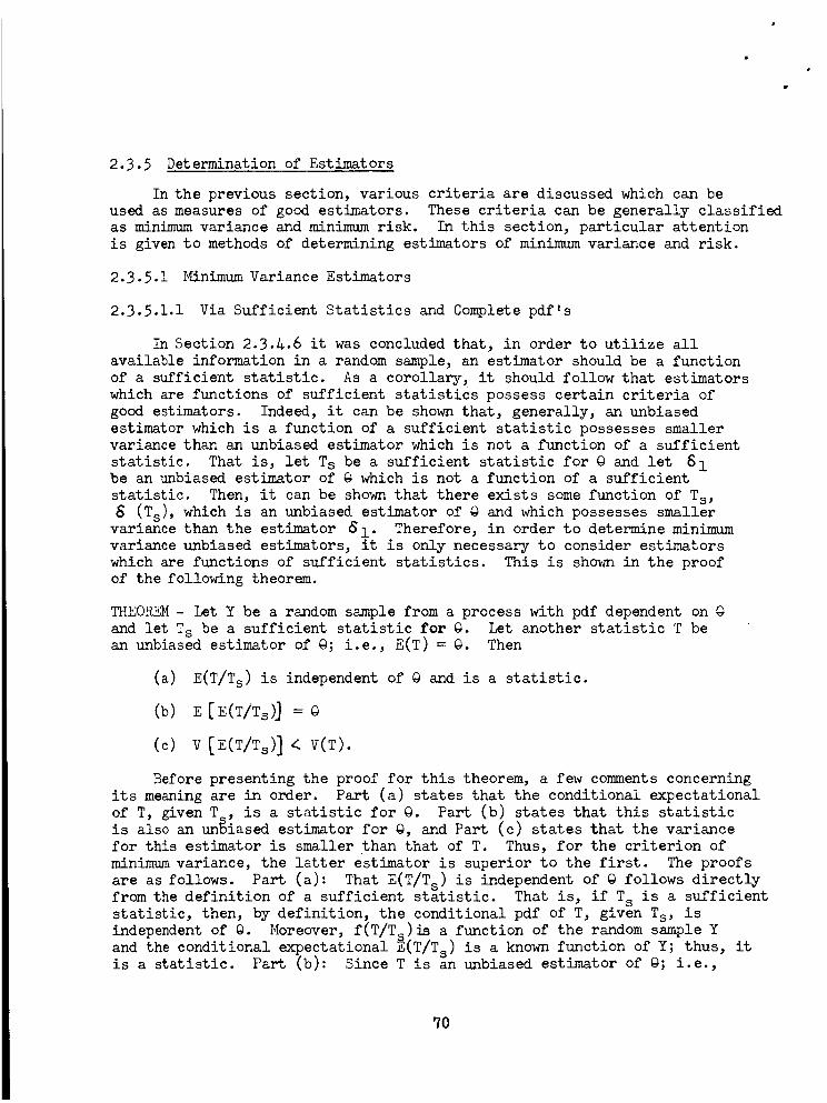
P
2.3.5 Determination of Estimators
In the previous section, various criteria are discussed which can be
used as measures of good estimators. These criteria can be generally classified
as minimumvariance andminimumrisk. In this section, particular attention
is given to methods of determining estimators of minimumvariance and risk.
2.3.5.1 Minimum Variance Estimators
2.3.5.1.1 Via Sufficient Statistics and Complete pdf's
In Section 2.3.A.6 it was concluded that, in order to utilize all
available information in a random sample, an estimator should be a function
of a sufficient statistic. As a corollary, it should follow that estimators
which are functions of sufficient statistics possess certain criteria of
good estimators. Indeed, it can be shown that, generally, an unbiased
estimator which is a function of a sufficient statistic possesses smallervariance than an unbiased estimator which is not a function of a sufficient
statistic. That is, let Ts be a sufficient statistic for @ and let _lbe an unbiased estimator of @ which is not a function of a sufficient
statistic. Then, it can be shown that there exists some function of Ts,
S (Ts), which is an unbiased estimator of @ and which possesses smaller
variance than the estimator gl. Therefore, in order to determine minimum
variance unbiased estimators, it is only necessary to consider estimators
which are functions of sufficient statistics. This is sho_m in the proof
of the following theorem.
THEOREM - Let Y be a random sample from a process with pdf dependent on @
and let Ts be a sufficient statistic for @. Let another statistic T bean unbiased estimator of @; i.e., E(T) = @. Then
(a) E(T/T s) is independent of @ and is a statistic.
(b) E[E(T/Ts)]=
(c) V [E(T/Ts) ] < V(T).
Before presenting the proof for this theorem, a few comments concerning
its meaning are in order. Part (a) states that the conditional expectational
of T, given T , is a statistic for @. Part (b) states that this statistic
is also an un$iased estimator for @, and Part (c) states that the variance
for this estimator is smaller than that of T. Thus, for the criterion of
minimum variance, the latter estimator is superior to the first. The proofs
are as follows. Part (a): That E(T/Ts) is independent of @ follows directly
from the definition of a sufficient statistic. That is, if Ts is a sufficientstatistic, then, by definition, the conditional pdf of T, given Ts, is
independent of @. Moreover, f(T/Ts)is a function of the random sample Y
and the conditional expectational E(T/Ts) is a known function of Y; thus, itis a statistic. Part (b): Since T is an unbiased estimator of @; i.e.,
7O
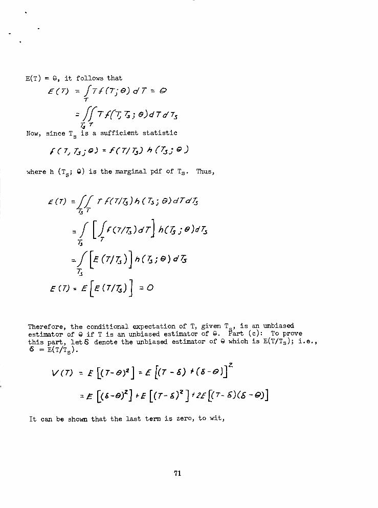
Q
E(T) = @, it follows that
E(O = /TS(T;e) dV = g_T
'//'T/fZ T,;e)dT"dTsT,T
Now, since Ts is a sufficient statistic
tel T_j_)= F(rl _j h (Tj;aJ
where h (Ts; @) is the marginal pdf of Ts. Thus,
_ (T) =_7_/ T I(T/T_)h ( Ts5 6_)d'TdTs
=/ [_Tf (7/Tz)af7"] h(Ta.; eJdTz
7_
E (7) = E IE (T/T_.) j -'0
Therefore, the conditional expectation of T, given T , is an unbiasedestimator of @ if T is an unbiased estimator of @. _art (c): To prove
this part, let _ denote the unbiased estimator of @ which is E(T/Ts); i.e.,
S = E(T/Ts).
It can be shown that the last term is zero, to wit,
71
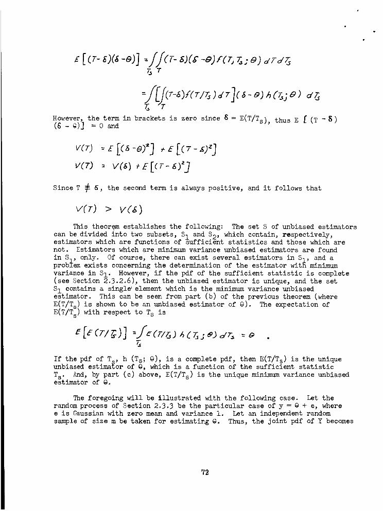
JdT ( D e >
However, the term in brackets is zero since 8 = E(T/Ts) ' thus E _ (T -8)(g - @)] = 0 and
VCT) : +z[cT-
Since T _ G, the second term is always positive, and it follows that
v('r) > v(g)
This theorem establishes the following: The set S of unbiased estimators
can be divided into two subsets, S7 and $2, which contain, respectively,estimators which are functions of _ufficient statistics and those which are
not. Estimators which are minimum variance unbiased estimators are found
in SG, only. Of course, there can exist several estimators in S1, and aprobIem exists concerning the determination of the estimator with minimum
variance in S1. However, if the pdf of the sufficient statistic is complete(see Section 2.3.2.6), then the unbiased estimator is unique, and the set
S1 contains a single _element which is the minimum variance unbiasedestimator. This can be seen from part (b) of the previous theorem (where
E(T/Ts) is shown to be an unbiased estimator of @). The expectation of
E(T/T s) with respect to Ts is
If the pdf of Ts, h (Ts; 9), is a complete pdf, then E(T/T s) is the unique
unbiased estimator of @, which is a function of the sufficient statistic
Ts. And, by part (c) above, E(T/T s) is the unique minimum variance unbiasedestimator of @.
The foregoing will be ±llustratedwith the following case. Let the
random process of Section 2.3.3 be the particular case of y = @ + e, where
e is Gaussian with zero mean and variance 1. Let an independent random
sample of size m be taken for estimating @. Thus, the joint pdf of Y becomes
72
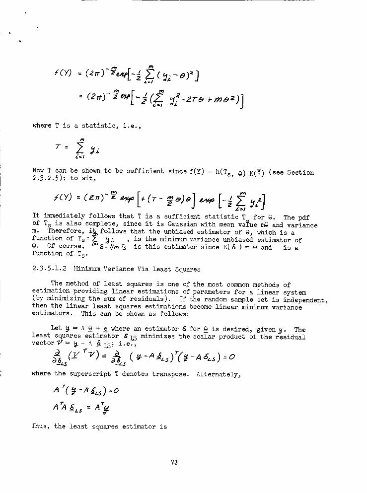
where T is a statistic, i.e.,
NowT can be shownto be sufficient since f(Y) = h(Ts, @)K(Y) (see Section2.3.2.5); to wit,
: Cz.) ('r- e)eIt immediately follows that T is a sufficient statistic T for @o The pdf
of Ts is also complete, since it is Gaussian with mean va_ue m@ and variance
m. Therefore, i_ follows that the unbiased estimator of @, which is a
function of T s , _ _z , is the minimum variance unbiased estimator of@. Of course, _='_://_T_ is this estimator since E(6 ) = @ and is a
function of Ts .
2.3.5.1.2 _nimumVariance Via Least Squares
The method of least squares is one of the most common methods of
estimation providing linear estimations of parameters for a linear system
(by minimizing the sum of residuals). If the random sample set is independent,
then the linear least squares estimations become linear minimumvarianceestimators. This can be shown as follows:
Let S = A _@+_e where an estimator _ for @ is desired, givens. The
least squares estimator SIS minimizes the scalar product of the residual
vector 17= __ A _ LS_ i.e.,
g
where the superscript T denotes transpose. ALternately,
Thus, the least squares estimator is
73
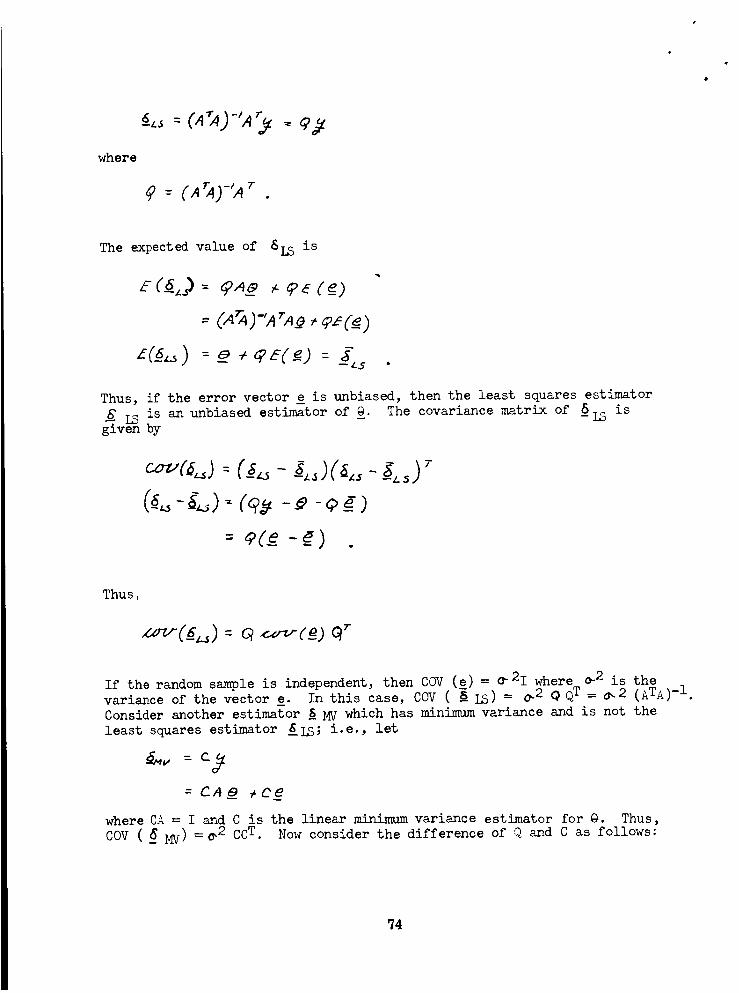
where
--(A_)-',__ .
The expected value of 6IS is
E ('6_.,)= 9,4_J-9E (_e)
- CA_)-,,_TA_,,?.(_)
Thus, if the error vector e is unbiased, then the least squares estimator
IS is an unbiased estimator of @. The covariance matrix of _LS isgivenby
7"
Thus,
If the random sample is independent, then COV (e) = _2I where _2 is the
variance of the vector e. In this case, COV ( _ iS) = _2 @ QT = _.2 (ATA) -1.
Consider another estimator _MV which has mini_mvariance and is not the
least squares estimator _LS; i.e., let
= CA_ +Ce
where CA = I and C is the linear minimumvariance estimator for @. Thus,COV ( _ D_) = @2 CCT. Now consider the difference of Q and C as follows:
94
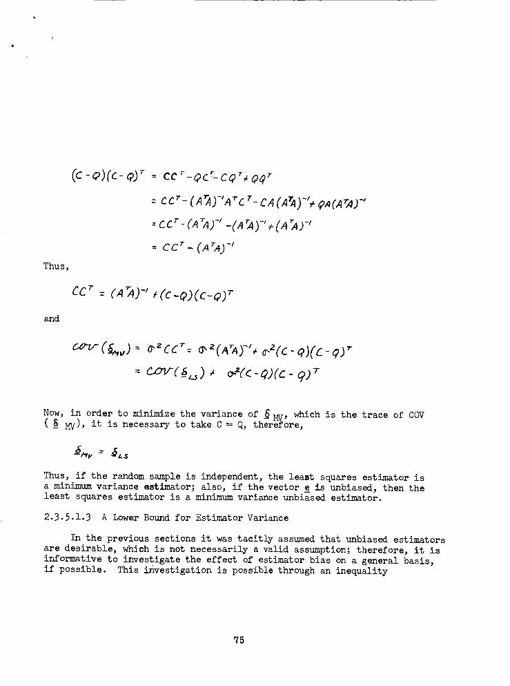
Thu s,
and
(c-Q)('c-Q.)7= cc _--cpc%cQ_,+¢_p_"
-:CCZ- (ArA)-'AT C T-CA(A_A)-% QA(A_) -,
: CCT-(A TA)-' _(ATA)-'+(A _)-/
= cc _- CA_A)-_
cc_ = (A-A)-',(C-Q)('C-_.)T
o,,cc": a,_(a%)-,,, _.2(c-_pj(_-_p)T
c.ov'( __u) ,, o,"(c-c])(c- c/) -r
Now, in order to minimize the variance of __}CC, which is the trace of COV( _S MV), it is necessary to take C = Q, therefore,
Thus, if the random sample is independent, the least squares estimator is
a minimum variance estimator; also, if the vector e is unbiased, then theleast squares estimator is a minimum variance unbiased estimator.
2.3.5.1.3 A Lower Bound for Estimator Variance
In the previous sections it was tacitly assumed that unbiased estimators
are desirable, which is not necessarily a valid assumption; therefore, it is
informative to investigate the effect of estimator bias on a general basis,
if possible. This investigation is possible through an inequality
75
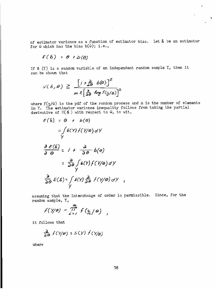
of estimator variance as a function of estimator bias. Let $ be an estimator
for @ which has the bias b(@); i.e.,
_ ( 8,) - e ,,b (_j
If 8 (Y) is a random variable of an independent random s_mple Y, then it
can be sho_n that
-->
where f(_/@) is the pdf of the random process and m is the number of elementsin Y. The estimator variance inequality follows from taking the partial
derivative of E(6 ) with respect to G, to wit,
E(,S) : _ ,, b('e)
:/_;c >o.,,'(>'/_)dyY
b e _e
/.;(yJ FC)I/QJ d) /= _-bY
--_cos)=/scy)_ sc>,/o)d>"Y
assuming that the interchange of order is permissible.
random sample, Y,
rOy�e) i= ,
Since, for the
it follows that
_--_,.cc>,/e) : ,sCy)Fcy/e)
where
76
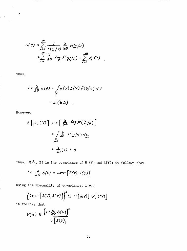
g,?
_rOy)--Z I _ s@je)m,m
_,#
Thus,
However,
Y
;E(SSJ .
;_e (I) -_.0
Thus, E( 8, S) is the covariance of _ (Y) and S(Y); it follows that
/F _#_ b(e) : _ [_(Y)>.E(y)3
Using the inequality of covariance, i.e.,
it follows that
7'7
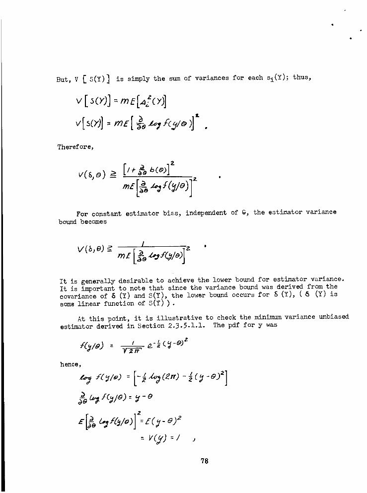
But, V [ S(Y)] is simply the sum of variances for each si(Y); thus,
Therefore,
,,,(._,_}___>[,, _: 6¢,,_]:
For constant estimator bias, independent of @, the estimator variance
bound becomes
!-- Z
_£
It is generally desirable to achieve the lower bound for estimator variance.
It is important to note that since the variance bound was derived from the
covariance of _ (Y) and S(Y), the lower bound occurs for S (Y), ( _ (Y) is
some linear function of S(Y) ).
At this point, it is illustrative to check the minimumvariance unbiased
estimator derived in Section 2.3.5.1.1. The pdf for y was
IC#i_J- _ o_-Ic_-_J_
hence,
"_J : [-s_-_-_-_]iC_le J -e_-__ : :v
: vC_J---I
78
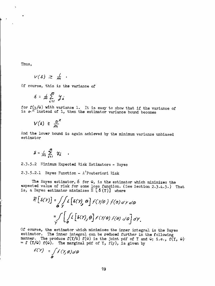
Thus,
!•
Of course, this is the variance of
_-I
for f_/@) with variance 1. It is easy to show that if the variance of
is _% instead of l, then the estimator variance bound becomes
v( j>
And the lower bound is again achieved by the minimum variance unbiasedestimator
2.3.5.2 l_nimumExpected Risk Estimators - Bayes
2.3.5.2.1 Bayes Function - AIPosteriori Risk
The Bayes estimator, 6 for @, is the estimator which minimizes the
expected value of risk for some loss function. (See Section 2.3./+.5.) Thatis, a Bayes estimator minimizes R [ 8 (Y)] where
Of course, the estimator which minimizes the inner integral is the Bayes
estimator. The inner integral can be reduced further in the following
manner. The produce f(Y/@) f(@) is the joint pdf of Y and 9,: i.e., f(Y, @)
= f (Y/Q) f(g). The marginal pdf of Y, f(y), is given by
ICY) :/i(_)de
7g
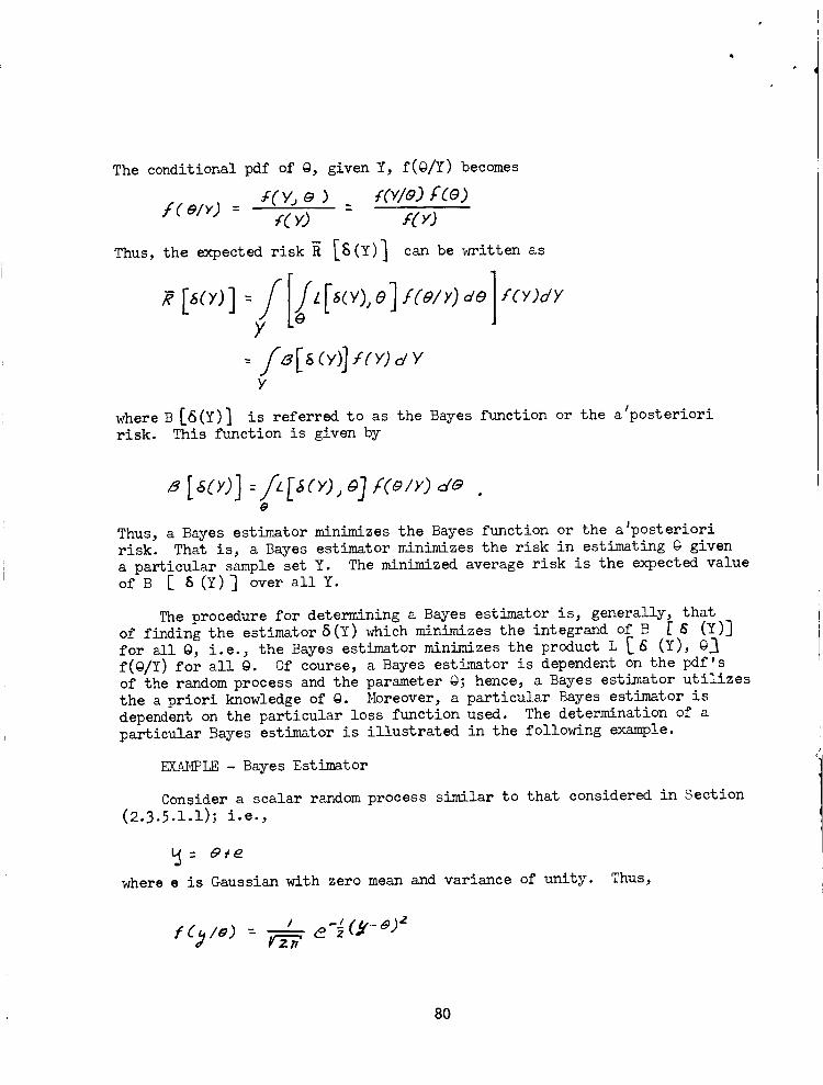
The conditional pdf of @, given Y, f(@/Y) becomes
S( Y, _, ) r(Y/_) f (O).f ( _/y) --
y) f( ×)
Thus, the expected risk R IS(Y)] can be written as
,[,<>,.>]Y
: Sz_[f, (Y)] f (Y) d YY
where B [6(Y)] is referred to as the Bayes function or the a#posteriori
risk. This function is given by
Thus, a Bayes estimator minimizes the Bayes function or the a_posteriori
risk. That is, a Bayes estimator minimizes the risk in estimating @ given
a particular sample set Y. The minimized average risk is the expected value
of B [ 8 (Y)] over all Y.
The procedure for determining a Bayes estimator is, generally, that
of finding the estimator 8(Y) which minimizes the integrand of B [ S (Y)]
for all @, i.e.j the Bayes estimator minimizes the product L [g (Y), @_
f(@/Y) for all @. Of course, a Bayes estimator is dependent on the pdf's
of the random process and the parameter g; hence, a Bayes estimator utilizes
the a priori knowledge of @. Moreover, a particular Bayes estimator is
dependent on the particular loss function used. The determination of a
particular Bayes estimator is illustrated in the following example.
EX_,_LE - Bayes Estimator
Consider a scalar random process similar to that considered in Section
(2.3.5.1.1); i.e.,
where e is Gaussian with zero mean and variance of unity. Thus,
l _I
8O
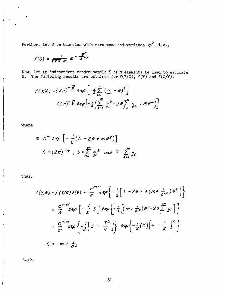
Further, let @ be Gaussian with zero mean and variance 0_2, i.e.,
t (e) - _ 6-
Now, let an independent random sample Y of m elements be used to estimate
@. The follo_ing results are obtained for f(Y/@), f(Y) and f(@/Y)o
" ZX.-_/
where
I
c--(2.;-", _ f * 2' : &" °"";: 2i:l Z=!
thus,
K K
./_ : r_+G, 2
Also,
81
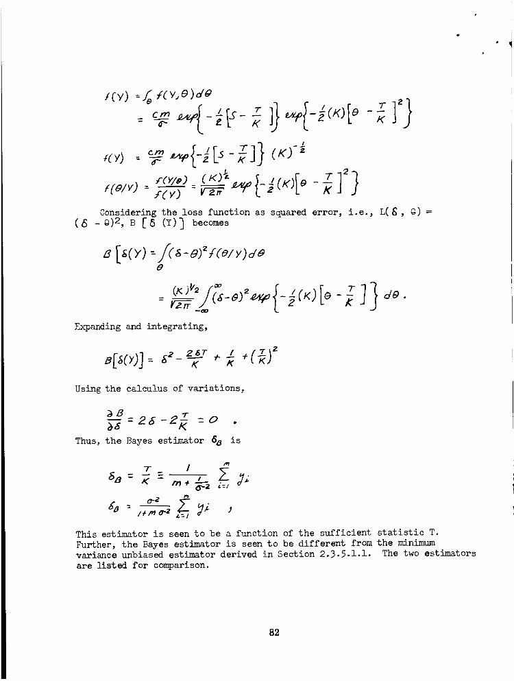
(8
/('Y) :J_e f(Y_e)°/@
_ _- __ - _ _ -_(K) e
I -/- ] J#C'/) c_ _2
Considering the loss function as squared error, i.e.,
- g) 2, B [8 (Y)_ becomes
L(S, 0) =
6
_ •E_qoanding and integrating,
Using the calculus of variations,
_B --r=25-2,_ =o .
Thus, the Bayes estimator 6a is
/_÷/L-
nil
This estimator is seen to be a function of the sufficient statistic T.
Further, the Bayes estimator is seen to be different from the minimum
variance unbiased estimator derived in Section 2.3.5.1.1. The two estimators
are listed for comparison.
82
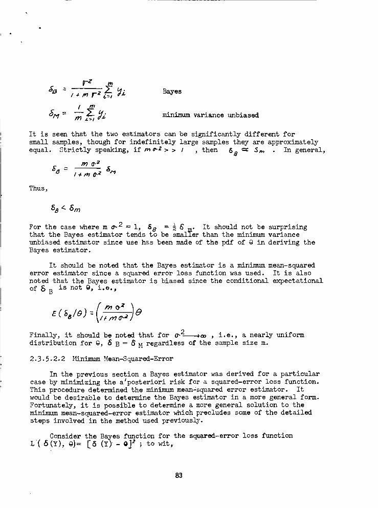
_-Z t.
I_ _ r z "= _,_ _yes
minimum variance unbiased
It is seen that the two estimators can be significantly different for
small samples, though for indefinitely large samples they are approximately
equal. Strictly speaking, if _ _z > > I , then 6 8 5_ In general,
Thus,
,58< 8m
For the case where m _2= i, S8 = -_l_" It should not be surprisingthat the Bayes estimator tends to be er than the minimum variance
unbiased estimator since use has been made of the pdf of @ in deriving the
Bayes estimator.
It should be noted that the Bayes estimator is a mininmmmean-squared
error estimator since a squared error loss function was used. It is also
noted that the Bayes estimator is biased since the conditional expectational
of S B is not @, i.e.,
E (4/a) : / @
Finally, it should be noted that for 0_2----._ , i.e., a nearly uniform
distribution for @, _ B = 8 M regardless of the sample size m.
2.3.5.2.2 _inimum Mean-Squared-Error
In the previous section a Bayes estimator was derived for a particular
case by minimizing the alposteriori risk for a squared-error loss function.
This procedure determined the minimummean_squared error estimator. It
would be desirable to determine the Bayes estimator in a more general form.
Fortunately, it is possible to determine a more general solution to the
minimummean-squared-error estimator which precludes some of the detailed
steps involved in the method used previously.
Consider the Bayes function for the squared-error loss function
L(6(Y), @)= [8 (Y)'- @]z ; to wit,
83
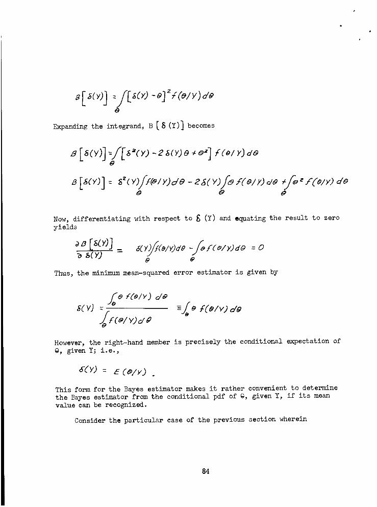
o
i
Expanding the integrand, B [ S (Y)] becomes
0
e e_
ore
Now, differentiating with respect to _ (Y) and equating the result to zero
yields
s(y) - e e
Thus, the minimum mean-squared error estimator is given by
f_oe f(_/y) c/eS(V) =
jF Cel YJd O-/w S(ely) Ja
However, the right-hand member is precisely the conditional expectation of
@, given Y; i.e.,
6&') : _ (a/y)
This form for the Bayes estimator makes it rather convenient to determine
the Bayes estimator from the conditional pdf of @, given Y, if its mean
value can be recognized.
Consider the particular case of the previous section wherein
84
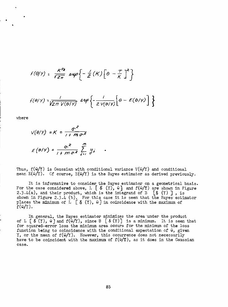
G
i
rCeiyJ - _. _ - _ (KJ e - -U_]
' {' t ]tf(e/>,J =V2r_ vCel_,J _y - z vCely.) e - ECeI×J
where
V(el×) =K -0.. 2
/÷ ,_Q,.z
Q, 2 f'_
Thus, f(@/Y) is Gaussianwith conditional variance V(@/Y) and conditional
mean E(@/Y). Of course, E(@/Y) is the Bayes estimator as derived previously.
It is informative to consider the Bayes estimator on a geometrical basis.
For the case considered above, L E g (Y), @] and f(@/Y) are shown in Figure
2.3.A(a), and their product, which is the integrand of B _8 (Y) 3 , is
shown in Figure 2.3._ (b). For this case it is seen that the Bayes estimator
places the mlnimum of L _ 8 (Y), @J in coincidence with the maximum off(_Iz).
In general, the Bayes estimator minimizes the areaunder the product
of L E 8 (Y), @] and f(@/Y), since B E 6 (Y)_ is a minimum. It is seen that
for squared-error loss the minimum area occurs for the minimum of the loss
function being to coincidence with the conditional expectation of @, given
Y, or the mean of f(@/Y). However, this occurrence does not necessarily
have to be coincident _th the maximum of f(@/Y), as it does in the Gaussian
case.
85
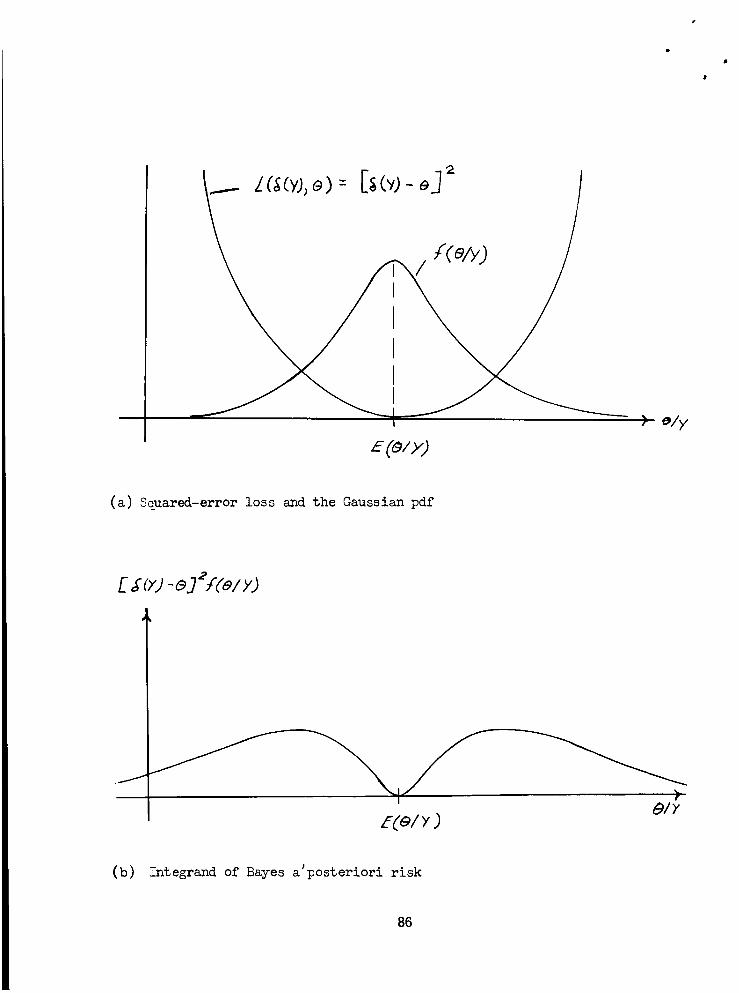
(a) Squared-error loss and the Gaussian pdf
E$(yJ-o]_i(al×)
.i
(b) Integrand of Bayes a'posteriori risk
80
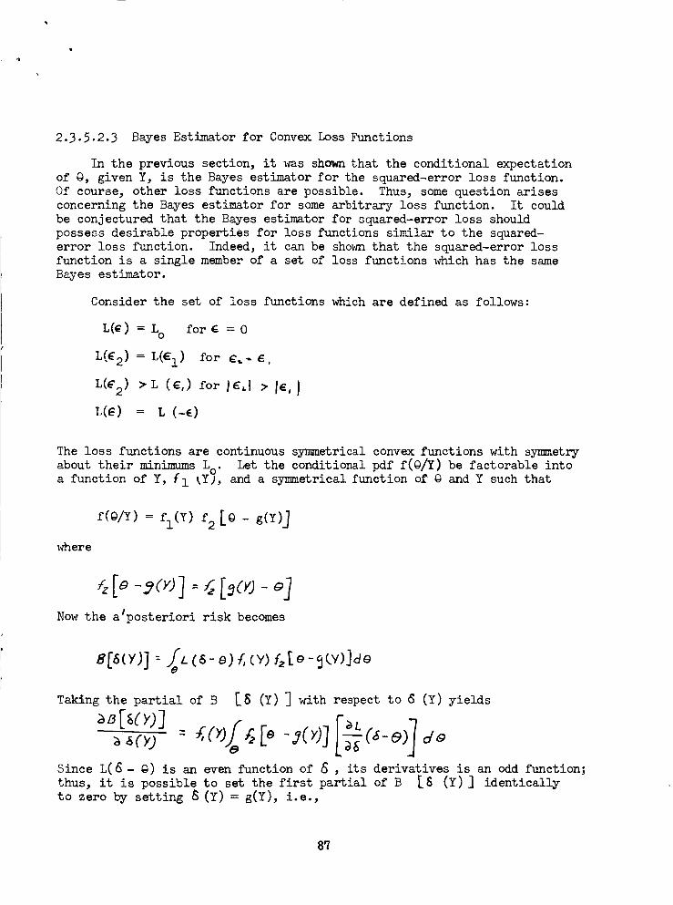
2.3.5.2.3 Bayes Estimator for Convex Loss Functions
In the previous section, it was shown that the conditional expectation
of @, given Y, is the Bayes estimator for the squared-error loss function.
Of course, other loss functions are possible. Thus, some question arises
concerning the Bayes estimator for some arbitrary loss function. It could
be conjectured that the Bayes estimator for squared-error loss should
possess desirable properties for loss functions similar to the squared-
error loss function. Indeed, it can be shown that the squared-error loss
function is a single member of a set of loss functions which has the same
Bayes estimator.
Consider the set of loss functions which are defined as follows:
L(_) = Lo for g = 0
L(E2) =L(el) for _.-_,
LCC2) >L (c,)for Ic, I • I_, }
L(G) = n (-E)
The loss functions are continuous symmetrical convex functions with symmetry
about their minimums L_. Let the conditional pdf f(@/Y) be factorable into• Q
a functlon of Y, fl tY), and a symmetrical function of @ and Y such that
f(9/Y)= fl(Y)f2[9 - g(Y)3
where
Now the alposteriori risk becomes
Taking the partial of B IS (Y) ] with respect to 6 (Y) yields
Since L(6- @) is an even function of _ , its derivatives is an odd function;
thus, it is possible to set the first partial of B [8 (Y) ] identically
to zero by setting 8 (Y) = g(Y), i.e.,
87
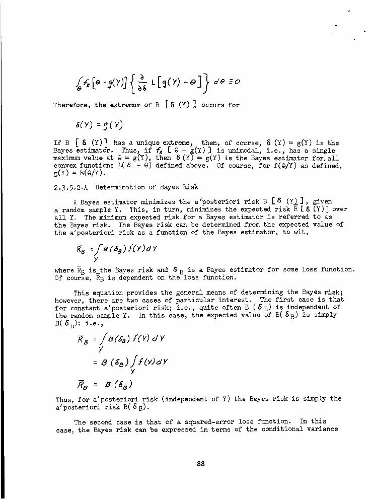
Therefore, the extremumof B [8 (Y) S occurs for
5(y.) : (,,,)
If B [ 8 (Y)_ has a unique extreme, then, of course, 8 (Y) = g(Y) is the
Bayes estimato_r. Thus, if ?cz [ @ - g(Y)] is unimodal, i.e., has a single
maximum value at @ = g(Y), then 8 (Y) = g(Y) is the Bayes estimator for. all
convex functions L( 6 - @) defined above. Of course, for f(@/Y) as defined,
g(Y) = E(g/Y).
2.3.5.2.A Determination of Bayes Risk
A Bayes estimator minimizes the alposteriori risk B [ 8 (y_)], given
a random sample Y. This, in turn, minimizes the expected risk R [ 8 (Y)] over
all Y. The minimum expected risk for a Bayes estimator is referred to as
the Bayes risk. The Bayes risk can be determined from the expected value of
the a_posteriori risk as a function of the Bayes estimator, to wit,
:jr ('58)f(>'JrJvY
where RB is_the Bayes risk and 6 B is a Bayes estimator for some loss function.
Of course, RB is dependent on the loss function.
This equation provides the general means of determining the Bayes risk;
however, there are two cases of particular interest. The first case is that
for constant a'posteriori risk; i.e., quite often B (6 B) is independent of
the random sample Y. In this case, the expected value of B(SB) is simply
B(6B); i.e.,
:/B(4,) f(Y) d YY
Y
Thus, for a_posteriori risk (independent of Y) the Bayes risk is simply the
a _posterior± risk B( 5 B).
The second case is that of a squared-error loss function. In this
case, the Bayes risk can be expressed in terms of the conditional variance
88
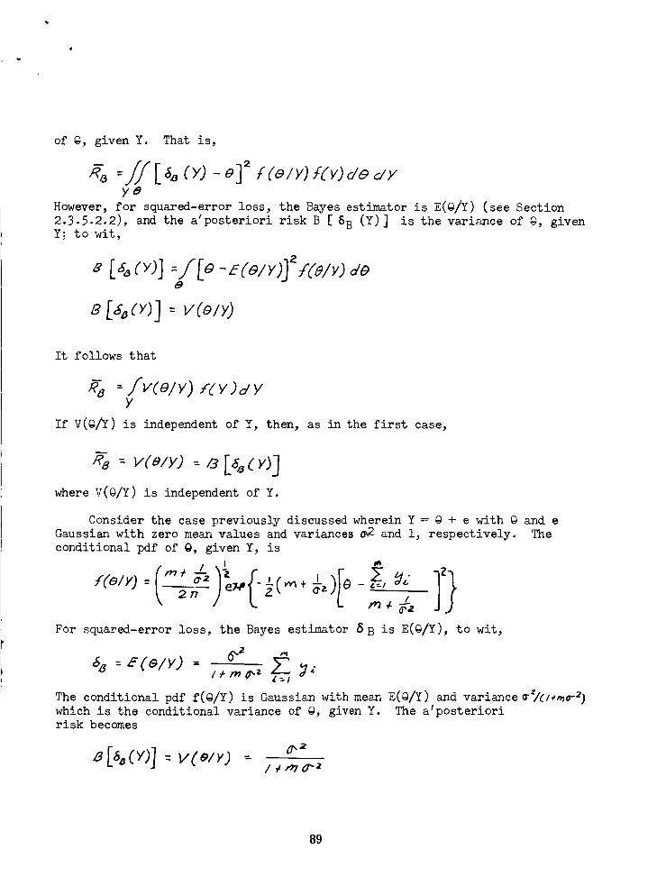
of g, given Y. That is,
ye
However, for squared-error loss, the Bayes estimator is E(O/Y) (see Section
2.3.5.2.2), and the a'posteriori risk B [ 6B (Y)] is the variance of @, givenY; to wit,
B [<r,,<>o]: vro<>,)
It follows that
-/v(o/y)/-<y)_,yY
If V(O/Y) is independent of Y, then, as in the first case,
: v<'ezyj --/3 [_ <>0_]where V(@/Y) is independent of Y.
Consider the case previously discussed wherein Y = @ + e with @ and e
Gaussian with zero mean values and variances 62 and l, respectively. The
conditional pdf of @, given Y, is
n
For squared-error loss, the Bayes estimator 8 B is E(g/Y), to wit,
,+..o.. 2Z _L=I
The conditional pdf f(g/¥) is Oaussian with mean E(g/¥) and variance #'/0÷_which is the conditional variance of @, given Y. The a_posterioririsk becomes
_2
/ ¢ ,,,_ 0"-2
89
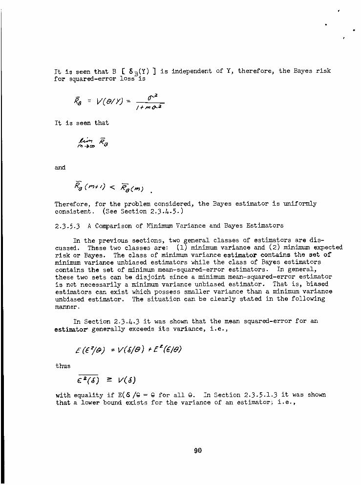
i
It is seen that B [ 8B(Y) ] is independent of Y, therefore, the Bayes riskfor squared-error loss is
-- v(e/zJ--
It is seen that
and
Therefore, for the problem considered, the Bayes estimator is uniformlyconsistent. (See Section 2.3.L.5.)
2.3.5.3 A Comparison of Minimum Variance and Bayes Estimators
In the previous sections, two general classes of estimators are dis-cussed. These two classes are: (1) minimum variance and (2) minimum expected
risk or Bayes. The class of minimumvariance estimator contains the set ofminimum variance unbiased estimators while the class of Bayes estimators
contains the set of minimum mean-squared-error estimators. In general,
these two sets can be disjoint since a minimummean-squared-error estimator
is not necessarily a minimumvariance unbiased estimator. That is, biased
estimators can exist which possess smaller variance than a minimum variance
unbiased estimator. The situation can be clearly stated in the following
manner.
In Section 2.3.A.3 it was shown that the mean squared-error for an
estimator generally exceeds its variance, i.e.,
ECE /, J : v(s/e ) , z" ( le)
thus
c=(<rj -="vC )
with equality if E(_/@ = @ for all @. In Section 2.3.5.1.3 it was shownthat a lower bound exists for the variance of an estimator_ i.e.,
90
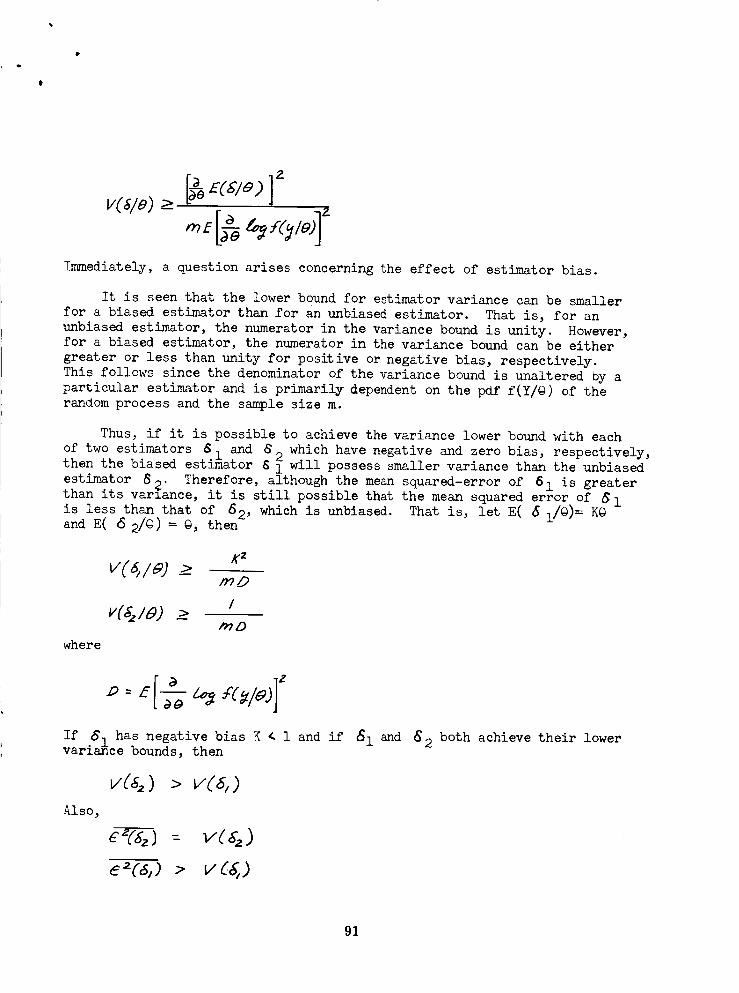
Q
@
Immediately, a ouestion arises concerning the effect of estimator bias.
It is seen that the lower bound for estimator variance can be smaller
for a biased estimator than for an unbiased estimator. That is, for an
unbiased estimator, the numerator in the variance bound is unity. However,
for a biased estimator, the numerator in the variance bound can be either
greater or less than unity for positive or negative bias, respectively.
This follows since the denominator of the variance bound is unaltered by a
particular estimator and is primarily dependent on the pdf f(Y/@) of the
random process and the sample size m.
Thus, if it is possible to achieve the variance lower bound with each
of two estimators 8] and 8 which have negative and zero bias, respectively,then the biased estimator 8 12will possess smaller variance than the unbiased
estimator 8@. Therefore, although the mean squared-error of 61 is greaterthan its varlance, it is still possible that the mean squared error of g 1
is less than that of 62, which is unbiased. That is, let E( 6 i/@)= K@
and E( 6 2/@) = @, then
K •
_D
I
where
If .S1 has negative bias K < 1 and if _l and g2 both achieve their lowervarzance bounds, then
Also,
v(,s,.) >
91
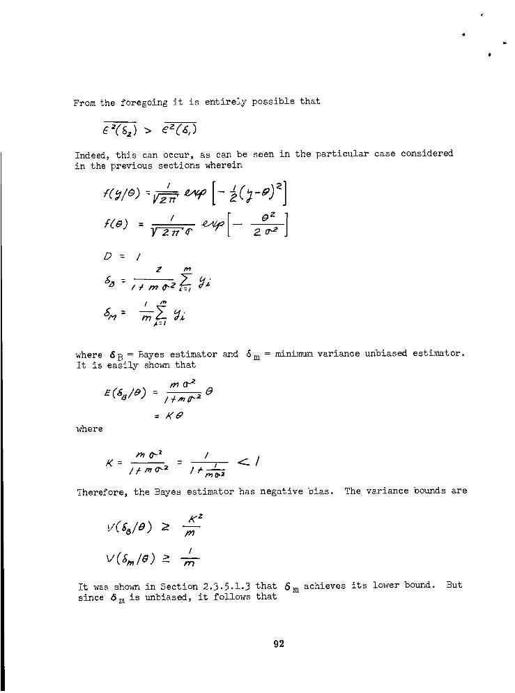
@
0
From the foregoing it is entirely possible that
Indeed, this can occur, as can be seen in the particular case considered
in the previous sections wherein
D -- /
Z m
I "_
_=I
where 8B = Bayes estimator and 6 m
It is easily shown that
where
= minimumvariance unbiased estimator.
/_ ma-2 i _ _-.-_
Therefore, the Bayes estimator has negative bias. The variance bounds are
K _
/,n
/
-- rn
It was shown in Section 2.3.5.1.3 that 6m achieves its lower bound. But
since 6 m is unbiased, it follows that
02
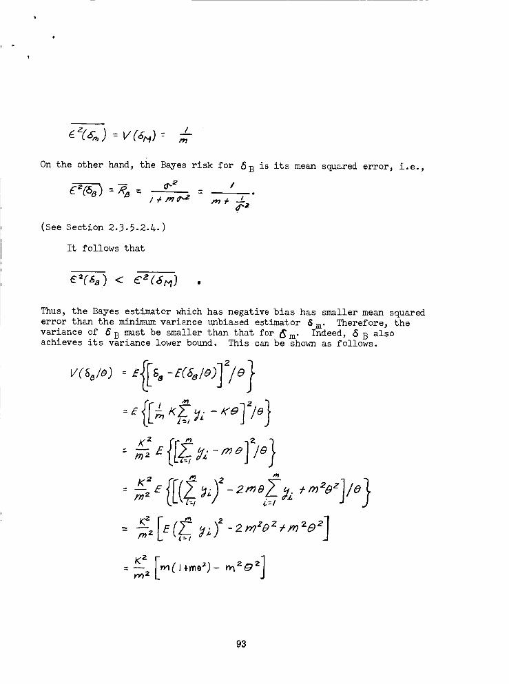
On the other hand, the Bayes risk for 6B is its mean squared error, i.e.,
(See Section 2.3.5.2.A.)
It follows that
¢_('8) < cz(a_) •
Thus, the Bayes estimator which has negative bias has smaller mean squared
error than the minimumvariance unbiased estimator 6 m" Therefore, thevariance of gB must be smaller than that for _m" Indeed, 8 B alsoachieves its variance lower bound. This can be shown as follows.
= maK--z[m('l+nn_a)_ ma_z I
93
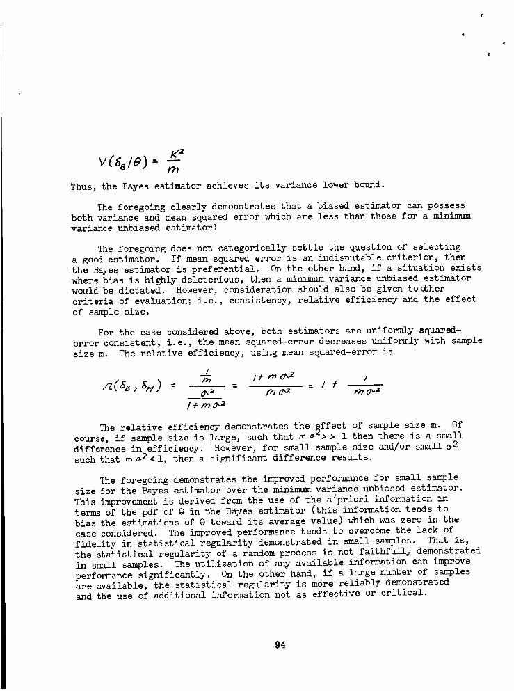
i
v¢6 1o).- K....=#99
Thus, the Bayes estimator achieves its variance lower bound.
The foregoing clearly demonstrates that a biased estimator can possess
both variance and mean squared error which are less than those for a minimumvariance unbiased estimator!
The foregoing does not categorically settle the question of selecting
a good estimator. If mean squared error is an indisputable criterion, then
the Bayes estimator is preferential. On the other hand, if a situation exists
where bias is highly deleterious, then a minimum variance unbiased estimator
would be dictated. However, consideration should also be given to_her
criteria of evaluation; i.e., consistency, relative efficiency and the effect
of sample size.
For the case considered above, both estimators are uniformly squared-
error consistent, i.e., the mean squared-error decreases uniformly with sample
size m. The relative efficiency, using mean squared-error is
I
- = / /- /
l + mo _a
The relative efficiency demonstrates the sffect of sample size m. Ofcourse, if sample size is large, such that m _> > 1 then there is a small
difference in efficiency. However, for small sample size and/or small @2
such that _ _2 < l, then a significant difference results.
The foregoing demonstrates the improved performance for small sample
size for the Bayes estimator over the minimum variance unbiased estimator.
This improvement is derived from the use of the a_priori information in
terms of the pdf of @ in the Bayes estimator (this information tends to
bias the estimations of @ toward its average value) which was zero in the
case considered. The improved performance tends to overcome the lack of
fidelity in statistical regularity demonstrated in small samples. That is,
the statistical regularity of a random process is not faithfully demonstrated
in small samples. The utilization of any available information can improve
performance significantly. On the other hand, if a large number of samples
are available, the statistical regularity is more reliablydemonstratedand the use of additional information not as effective or critical.
94
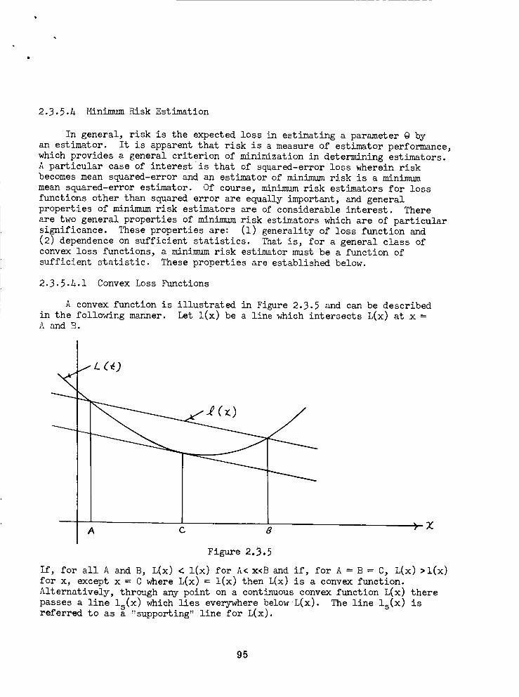
2.3.5.& _nimum Risk Estimation
In general, risk is the expected loss in estimating a parameter @byan estimator. It is apparent that risk is a measureof estimator performance,which provides a general criterion of minimization in determining estimators.A particular case of interest is that of squared-error loss wherein riskbecomesmeansquared-error and an estimator of minimumrisk is a minimummeansquared-error estimator. Of course, minimumrisk estimators for lossfunctions other than squarederror are equally important, and generalproperties of minimumrisk estimators are of considerable interest. Thereare two general properties of minimumrisk estimators which are of particularsignificance. Theseproperties are: (1) generality of loss function and(2) dependenceon sufficient statistics. That is, for a general class ofconvex loss functions, a minimumrisk estimator must be a function ofsufficient statistic. Theseproperties are established below.
2.3.5.&.1 ConvexLoss Functions
A convex function is illustrated in Figure 2.3.5 and can be describedin the following manner. Let l(x) be a line which intersects L(x) at x =A and B.
/ L ('U
Figure 2.3.5
If, for all A and B, L(x) _ l(x) for A<x<B and if, for A = B = C, L(x) >l(x)
for x, except x = C where L(x) = l(x) then L(x) is a convex function.
Alternatively, through any point on a continuous convex function L(x) there
passes a line is(X) which lies everywhere below L(x). The line ls(X) isreferred to as a "supporting" line for L(x).
95
An important property of a convex function of a random variable is
that its expectation generally exceeds its value at the expectation of therandom variable; i.e., if L(x) is a convex function and x is a random variable
then
This can be shown as follows: Let ls(X) be a supporting line of L(x) at
the point E(x). Thus
LCx),>__ (x)and
However, since is(X) is linear in x E [ is(X) ] = is [ E(x)J thus,
,_ELr,,o-I->___IE_'x.).lMoreover, since Is(X) supports L(x) at E(x), L [ E(x)] = Is [ E(x)] thus,
cxJJ z i- cxJJ.As a particular case consider x as estimation error
squared error loss,: i.e.,
and L( _ ) as
L (c) : c _'It follows that
El_,_c_J]: _t'_:J->[,c_.)]:This result agrees with that of Section 2.3._.3 wherein it was determined
that
E (e") : v (E) ,, E "(_)on
(eD z z:_(E)
with equality for V( g ) = 0 which implies a constant c.
The preceding inequality of convex function expectation is fundamental
96
to showing the necessity of sufficient statistics for minimumrisk estimators,which is considered below.
2.3.5._.2 Iv_nimumRisk Via Sufficient Statistics
In Section 2.3.5.1.1 it was shownthat if T and Ts are an unbiasedestimator and a sufficient statistic for @,respectively, then E [ E(T/Ts)]is an unbiased estimator for @;and the variance of E(T/Ts) is less thanthe variance of T. Theseresults can be generalized in two respects. First,any function of @,U(@), canbe considered; and, second, variance can bereplaced by risk for convexloss functions. Theseresults will be proved inthe following theorem, which is an extremely important extension of thetheorem of Section 2.3.5.1.1 concerning sufficient statistics and minimumvariance estimators. In effect, this theoremdemonstratesthe fundamentalimportance of sufficient statistics in determining estimators.
THEORY4:Let Y be a randomsamplefrom a process with pdf dependenton @,and let Ts be a sufficient statistic for @. Let T be another statisticwhich is an unbiased estimator for any function of @,U(@); i.e., E(T) = U(@).Then
(a) E(T/Ts)is independent of @and is a statistic
(b) = U(O)
(c) R(T, : R( s,
where the risk is for convex loss functions and 8Ls = E(T/Ts).
Before proving this theorem, two comments are in order. First, it
should be noted that biased estimators for @ are included since an unbiased
estimator of U(@) includes a biased estimator of @; i.e., the case U(@) = k_
where k _ 1 is included. Second, 6 Ls is anunbiased estimator of U(@), or a
biased estimator of' @, and 8Ls is an estimator which has less risk than Tfor all convex loss functions.
The proofs of parts (a) and (b) of the theorem are direct extensions
of the proofs given in Section 2.3.5.1.1. Part (a) is an obvious extensionand part (b) follows.
97
E (_)- _(e)
=_r f Cr 5 eJ_r
: S ?T f (_ _ j e) dTEr_
=/_TICT/rj)6 ( _ 5 e) drd 5rj r
-- -
Part (c) follows from the property of expectation of convex functions as
shown in the previous section. Let L( 2, Q) be a convex loss function with
respect to the unbiased estimator 6 for U(Q); i.e., for fixed Q, L(_ , @)
is a convex function of 6 • Taking the conditional expectation of L( S, @),
given Ts, it follows that
_> /_ (6_ ,o)
Taking the expectation over all Ts it is found that
Therefore,
The foregoing is extremely important since it establishes that minimum
risk esti_.ators are functions of sufficient statistics and, thus, only
sufficient statistics need be considered in determining minimum risk estimators.
Furthermore, if the pdf of Ts is complete, then the unbiased estimator 8 sof U(@) which is a function of Ts is unique and the estimator of minimum
9a
risk for the class of convex loss functions. These results representextremely important extensions of the significance of sufficient statisticsin determining estimators.
2.3.5.5 Maximum Likelihood Estimators
In general, maxinmm likelihood estimators are determined by maximizing
a pdf. This method of estimation does not explicitly seek to satisfy criteria
of estimation, rather, the method is based upon the premise of the most
probable occurrence being observed most frequently. In effect, it is
assumed that a random sample is always one of high relative probability.
Nonetheless, the method is often equivalent to other methods of determiningestimators, and similar results are often obtained. The method is discussed
herein to show its significant similarities and differences with othermethods.
2.3.5.5.1 Principle of Maximum Likelihood
The principle of maximum likelihood is predicated upon a "most likely
occurrence" of a set of variables. In general, a pdf is a relative measure
of the probability of occurrence of its variable. The particular set of
variables for which the pdf is a maximum can be considered as a maximum
likelihood set. Any pdf associated with a set of variables is considered
to be a likelihood function for the set of variables; e.g., the pdf'sf(@/Y) and f(Y/@) are likelihood functions for the variables @ and Y. If
the likelihood function possesses a maximum value, then the particular set
of variables for which the maximumvalue occurs is the set of most likelyoccurrence or maxinmm likelihood. This set of variables is referred to
as the "mode" of the likelihood function or pdf of the set of variables.
The principle of maximum likelihood leads to the following method of
estimation, which is based on maximizing a pdf as a function of a set of
parameters @.
2.3.5.5.2 Maximum-Likelihood Estimator
Let the likelihood function for a random sample Y be some pdf for Y
as a function of a set of parameters 9. If the likelihood function has
a maximum value for @ (@ is some function, 8 (Y), of the random sample, Y),
then 6 (Y) is the maximum-likelihood estimator of @. Thus, the maximum-
likelihood estimator for @ is the one for which the random sample Y occurs
with maximum likelihood.
The method of maximum-likelihood estimation is depicted in Figure
2.3.6.
99
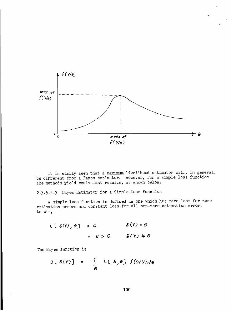
f ( y/e)
j I0 i L.
f[ Ylo )
It is easily seen that a maximum likelihood estimator will, in general,
be different from a Bayes estimator. However, for a simple loss function
the methods yield equivalent results, as shown below.
2.3.5.5.3 Bayes Estimator for a Simple Loss Function
A simple loss function is defined as one which has zero loss for zeroestimation errors and constant loss for all non-zero estimation error;
to wit,
L [. ,_(Y)_ e.] = o _(Y) = e
- K> 0 ,_(Y.) _e
The Bayes function is
._ LE ,S,e'l f('elY,)c/e
lOg
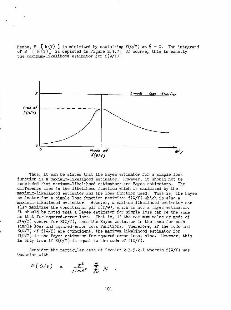
Hence, B [ $(Y) _ is minimized by maximizing f(@/Y) at S = @. The integrand
of B [ 8 (Y) J is depicted in Figure 2.3.7. Of course, this is exactly
the maximum-likelihood estimator for f(@/Y).
K
o m_e oF"+Y_/y)
_y
Thus, it can be stated that the Bayes estimator for a simple loss
function is a m_ximum-likelihood estimator. However, it should not be
concluded that maximum-likelihood estimators are Bayes estimators. The
difference lies in the likelihood function which is maximized by the
maximum-likelihood estimator and the loss function used. That is, the Bayesestimator for a simple loss function maximizes f(@/Y) which is also a
maximum-likelihood estimator. However, a maximum likelihood estimator can
also maximize the conditional pdf f(Y/@), which is not a Bayes estimator.
It should be noted that a Bayes estimator for simple loss can be the same
as that for squared-error loss. That is, if the maximum value or mode of
f(@/Y) occurs for E(@/Y), then the Bayes estimator is the same for both
simple loss and squared-error loss functions. Therefore, if the mode and
E(@/Y) of f(@/Y) are coincident, the maximum likelihood estimator for
f(@/Y) is the Bayes estimator for squared-error loss, also. However, this
is only true if E(@/Y) is equal to the mode of f(@/Y).
Consider the particular case of Section 2.3.5.2.1 wherein f(@/Y) wasGaussian with
( a / y) : ,r___2"
101
The maximum of f(@/Y) occurs at E(@/Y), therefore, the Bayes estimator is
the same for both simple and squared-error loss. It is easily shown that
the maximum likelihood estimator for both f(@/Y) and f(Y, @) are E(@, Y);
however, if the likelihood function f(Y/@) is used, then the maxin_im likeli-
hood estimator is the same as the minimum variance unbiased estimator,
i/__C_=I,_ determined in Section 2.3.5.2.1.
In general, if the likelihood function is dependent on the a priori
pdf for @, then the maximum likelihood estimator is the same as the Bayesestimator for a simple loss function, and both estimators utilize the
a Spriori information available concerning @. If, on the other hand, thelikelihood function is independent of the pdf for @, the a_priori infor-
mation concerning @ is not utilized. However, it should not be concluded
that Bayes estimators can generally be derived by the method of msodnuumlikelihood.
2.3.6 Application of Bayes Estimation
2.3.6.1 Introduction
The discussions of the previous sections have established the criteria
of value in defining estimators and measures of the "goodness" which results.
This section is intended to conclude the discussion of estimation by
applying the most general of the previously developed estimators (Bayes)
to the general non-linear estimation problems. This application will,
however, fall short of providing computational algorithms which can be
utilized in analyses since the pdf's for the variables involved and the
functional relationships between them must be specified. Thus, the special
case of the general linear system of equations and Gaussian statistics will
be developed.
2.3.6.2 Non-Linear Case
The general case of interest is defined by the follov_ng vector
equation: (See Section 2.3.3.)
The parameter vector @ contains n elements, and an estimator for each
element is required. Thus, an estimator is denoted by the vector 6_.
Estimation error is like_lse a vector defined by
A loss function for the estimation error vector _____is defined as a scalar
function of some positive definite measure of the modulus of g__; e.g.,
sum-squared-error, SSE, is a particular loss function which is defined by
102
or
Lsl
where T denotes transpose.
A more general loss function is defined in terms of the squared modulus
of a linear transformation of __.; i.e.,
L c 6
= gTME
where B is some linear transformation and M is a real symmetrical matrix.
In this case, L(E_) is a generalized quadratic loss function which is a
positive semi-definite function with L( E ) - 0 if, and only if, E__ ---0
for B _ O. Of course, for M = I, L(E__)-_--SSE = __T___.
In general, L(E__) is a function of m_ and @_; i.e., L(g ) = L(S__, @_).
For generalized quadratic loss, L(8___,@_) becomes
Note. This form exists because each of the terms involved is a scalar.
The Bayes estimator _-B for generalized quadratic loss is the vectorof estimators which minimize the expected risk or the a'posteriori risk,
as discussed in Section 2.3.5.2. The Bayes function for this loss is
The Bayes estimator Z_-B can be found by differentiating B ES..(_.)] with
respect to 8 and equating to zero, to wit,
103
The resulting axpression can be made identically zero for all n if
or
A =SerC_-i_J<tesince
Thus, it is seen that for a generalized quadratic loss function the Bayes
estimator__.B is the conditional expectation of @_ given Z; i.e.,
g..-8 -i _ f (_.l_d_ :E (_a/_.) .
This result is equivalent to that determined in Section (2.3.5.2.2) for the
explicit case of a single parameter @.
The Bayes risk _B for 8 B is the expected value of B(g_B) over all _L,
ice°)
= _ {e[_.c'__,_>s>/#.])For generalized quadratic loss, the Bayes risk becomes
104
If B(_B ) is independent of y, then
It should be emphasized at this time that the results given above are
not restricted to the linear case since the explicit form of the process
does not enter into the determination of the Bayes estimator as the con-
ditional expectation of @, given X. However, it should be noted that the
form of the process, as determined bye(@), definitely enters into the
determination of the E(@_/X); and, therefore, the Bayes estimator is dependent
on the form of the process. That is, the conditional expection of @, given
X, is the Bayes estimator for a generalized quadratic loss function for any
functional relationship of @ and Z- On the other hand, the specific form
of the Bayes estimator is dependent on the form of _(@). Further, the
Bayes estimator can be a non-linear function of the observation vector X.
Moreover, the Bayes estimator for a particular case is dependent on the
statistics involved; i.e., the pdf's f(@), and f(e__). Thus, it can be
concluded that for a generalized quadratic loss function the conditional
expectation of @, given X, is the Bayes estimation which willminimize the
expected risk. In a particular case, the specific form of the Bayes estimator
is determined by the form of the process, _(@), and the statistical nature
of @ and ___ as reflected in their pdf's.
The determination of a Bayes estimator for the general case can be
formulated by determining the conditional pdf, f(@_/X), and its conditional
expectation. This procedure will be outlined for the case that the
statistical nature of @ and c must be known; i.e., the pdf's f(@) andf(e__) are assumed available, m
105
First, the conditional pdf of y, given @, is determined by considering
F(@_) as a constant in the process y = F_(@_)+-_. Thus, f(z/_@) is derived
from f(e__) by including the additional term _F__) in the expected value of
_G_.
Second, the joint pdf of y and @, f(_/@) is formed. For the mostcommon situation of statistically inSepen_e_t @_ and e, f(z/@_) f(_@).
Third, the marginal pdf of y, f(z), is determined by integrating f(y, @_)
over all @, to wit,
ae
Fourth, the conditional pdf of 9, given Z, is formed by the standard
form for conditional pdf's, to _rit,
=l /o_1
Fifth, the conditional expectation of @_, given y, is determined from
f(@, y). Once f(@_/y) is determined, it is often possible to recognize the
E(@_/yV by inspection; and, hence, the Bayes is directly determined. Other-
wise_ the general approach is to determine the conditional expectation by
integrating, to wit,
The degree of difficulty in determining a Bayes estimator is
directly related to the nature and degree of complexity of the functional
form of _F(@_)which significantly affects the determination of f(y). Moreover,
the form of the pdf's f(e) and f(@_) affect the determination of a Bayes
estimator; and often the task can be somewhat difficult. However, the approach
provides a general method of determining the optimum estimator using minimum
expected risk as primary estimation criterion for generalized quadratic loss.
In general, it is to be expected that the Bayes estimator will be a
non-linear function of y, even in the case for a linear form of F(@_) = A@_,
depending on the statistical nature of @_ and e. However, quite often it is
highly desirable to utilize a linear estimator; and under such a constraint,
the resulting estimator will not be a Bayes estimator though it is possibleto determine the linear estimator which will minimize the expected risk.
Such estimators would be sub-optimal in the sense that the Bayes estimator
wouid possess uniformly smaller risk. The use of sub-optimal linear estimators
must be considered on the basis of particular problems if the utilization
of a non-linear estimator presents a difficult situation in terms of data
processing an estimator mechanization in other respects.
106
On the other hand, the Bayes estimator can be a linear function of 2;
and in such cases, no particular problem arises. This is particularly true
for linear systems with Gaussian statistics. This case is of general interestand is discussed in detail below.
2.3.6.3 linear Case, Gaussien Statistics
The general linear case is defined by _(Q) = A@, i.e., _ = A@ + e,
where A is a known matrix independent of _. However, A can be time dependent
or, generally, non-stationary. For the case of Gaussiar, statistics, it can
be sho_n that the Bayes estimator is a linear function of Z. This particularcase is of general interest and is derived in detail herein.
The pdf's for _@ and e are assumed to be n and m dimensional multi-
variate Gaussian pdf's _._th the follo_ng specification:
_(_e)= To
v(o)-E(_e-_,,)(.o_%)r
V(e)= _(e_-_,)(e___,)T
_,h_re, of course, V(@) and V(e) are the covariance matrices of @ and e,respectively.
Further, the pdf's f(v_/@_), f(y, @_), f(z) and f(@_/Z), where @_ and
e are assumed as statistically independent are:
: xp J v- o,where
C
I
,t' = ._ -Ae - _me = .,_ - A_O _-A _-e - m_ = (+e' - m_ ) -A (@ -_)
} V(e) I = determlnamt of
/'_¥, o) : ,"c_/# ) •r(o)
v(_)
10'1
Rather than integrating f(y, @_) over all _@ to obtain f(y)_ it is easier
to use the fact that Z is the linear sum of two independent Gaussian randomvariables, hence,
E(_= ___= A__e +,_
_ )T
=,4 V(B.)A T+ V(e)
It follows that
r(_) =c_lv_J exp[-_-(_-___fv_{_-___]
_ow
Hence
/ . )]
where
and
_ _ _ V_ _W _Q(e,_;=CW-,_VFV_e)(W_-AV)÷ V_e)v_ _ VC_f)W
V.=g-__ e
The term Q(_, y) specifies the conditional Gaussian pdf f(__/y), and itsgenera 1 form is
108
where V(@/y) is the conditional covariance matrix of _ given y. Thus, in
order to determine the Bayes estimator, it is only necessary to determine
the reduced quadratic form for Q(@_, y).
Expanding Q(@_, x) in terms of _ and E, it is found that
Q+o_,++:_v"[v-t.o++._v+°_,,]_v-,+v_"v+°_v.,-_+"[v",.+,-,,-:,_.j]+=<y - _WJ r vte/?)(_v-_ W)
where K and V-1 (@/y) must be determined. It should be noted that the term
K essentially determines the Bayes estimator since
c_v-_+__:[+-++]
Thus, the Bayes estimator is
s_B = _(o/_)
s_8 - _ + _:(._-m_).
The term K can be determined by expanding the second expression for
+_(£,z)
Qce,_)= y" v"(o/_)v-zv'v-to/g)_w+w'_.'v"(e/f)v._
and by equating terms in the two _::'_+-;: _s
v-'co/_): [v_o_+,-A"v"_a]
109
Thus, it is found that two solutions exist for K. The second equation yields
K, ---V_Ol,t) N V '(e)
Substituting the second eauation into the third, it is seen that
V,.'rAT= V (e) [ V'_('e)-V-_'_)]
= I - V(e) V"(_)
Taking the transpose and substituting V(e) = V(y) - AV (@) AT,
that
it is found
Thus,
k:,: vce) v-I )
The two solutions for K generally imply two Bayes estimators for the case
being considered; however, it "will be shown later that the Bayes estimator
is unique and that K1 and K2 represent two equivalent forms of the sameestimator.
Several comments concerning the Bayes estimator for this case are in
order. It is seen that the Bayes estimator for this case is a linear function
of Z; thus, _-B is a linear estimator.
The matrix K is a "gain" matrix which, in effect, specifies the
weights in estimating @ that are given to the deviations in the observed
Z from its mean value _my. If the mean value _ is actually observed, then
the Bayes estimate for-_ is the mean value of __; i.e., for Z =_, /L-B = _-
On the other hand, if the observed Z is identically zero, then t_e Bayes
estimate for @ weights the mean value of _ by the gain matrix K to form the
estimate of @; i.e., for _ _ 0
110
In general, the deviations of observed Z from_my are weighted by K toform the Bayes estimate____B as shown. It is easily_shown that 8B is abiased estimator, to wit,
r (__s/__)= "%, k:[Ec_.ze)- _t']
Of course, if KA = I, then E(gu/@) = @; and _-B would be unbiased. It isinteresting to note that if V_ = O. Which implies a constant e = n_, then
v-l(y) = (AV(@) AT)-l and KA = V(@)A T (AV(@)AT)-lA = I, where A=l ex-ists.
However, in this case
or
: v<e>A"[Av<,,m]-'
: +A _ :e
= % +E(._- _t)
This is to be expected since,
determined exactly.
if e is a known constant, then @ can be
In general, V(e) _ O, and an error eeB exists in the Bayes estimate.
The Bayes error ____Bis
___ = _S_-__
: _me ÷K(_-_)-_
- _e -_e ÷_c(g-__)
_-s : (z - KA)(e - _e)' _(e- - ___)
The conditional expectation of __eB, given @, is thus
111
B
-(__-o)+KA(__-__)
E(:a/e.) = (I-KA)(_8- m_) .
The total expectation of _--B is zero; i.e.,
a-(._%)-- o
The covariance matrices for 6___Band W_B can be readily derived and one found
to be equal, to wit,
where
and, likewise,
.
Thus, _ - E(___BI@) = _ - E(EBI@), and it follows that V(BB ) = V(6 B)"The covariance matrices for $ B _n_ _B can be determined in explicit form
by using the conditional expectation of iB, given _, to wit,
112
i
i
Now,
-, {[-_-'¢_,'_,._][o-,u_,'_.O%}
II(E s I_) " { V-'(e.) # A" U'teJ A )-/ o
Thus,
v%J : E V(E,_I._)
vcEs_: ( v-'@j+A_v-'C<J_)-' .
Thus, the covariance matrices for 8_B and _---Bare actually independentof K and are essentially dependent on the intrinsic aspects of the problem;
i.e., the covariance matrices of the parameters, @; the measurement errors,
e; and the transformation, A, of parameters @ into observables, X"
The Bayes risk can now be determined as follows: first, the generalized
quadratic loss function is constructed
Z(_¢) :£__E
: ('_,, -_ej%(_%-_j
113
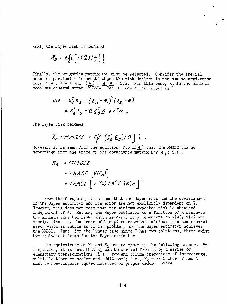
Next, the Bayes risk is defined
Finally, the weighting matrix (M) must be selected. Consider the specialcase (of particular interest) wherethe risk desired is the sum-squared-errorloss; i.e., M= I and L(___)= ET_ = SSE. For this case, RB is the minimummean-sum-squarederror, M_%SE.---T_eSSEcan be expressedas
=_r z
The Bayesrisk becomes
However, it is seen from the equations for L(g_) that the I,_SE can bedeterminedfrom the trace of the covariance matrix for e B; i.e.,
= MM SS£
--rRAcE rv%>]
- tRAcE[ v-t'o. -,
From the foregoing it is seen that the Bayes risk and the covariances
of the Bayes estimator and its error are not explicitly dependent on K.
However, this does not mean that the minimum expected risk is obtained
independent of K. Rather, the Bayes estimator as a function of K achieves
the minimum expected risk, which is explicitly dependent on V(@), V(e) and
A only. That is, the trace of V(_ B) represents a minimum-mean sum squared
error which is intrinsic to the problem, and the Bayes estimator achieves
the _SE. Thus, for the linear case since K has two solutions, there exist
two equivalent forms for the Bayes estimator.
The equivalence of K1 and K2 can be shown in the following manner. By
inspection, it is seen that K1 can be derived from K2 by a series ofelementary transformations (i.e., row and column operations of interchange,
multiplications by scalar and additions); i.e., K2 = PKIQ where P and Q
must be non-singular square matrices of proper order. Since
114
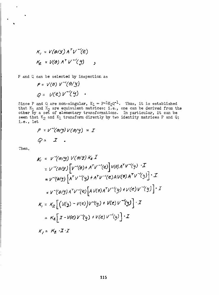
i
K,- vCe/.v)A_V-'(_)
.i
P and Q can be selected by inspection as
p = v(e) v-'(el_.V.)
_p- vde.)v-'_2) •
Since P and Q are non-singular, KI = p-IK2Q-I.
that K1 and K2 are equivalent matrices; i.e.,other by a set of elementary transformations.
seen that K2 and K1 transform directly by two identity matrices P and Q;i..e., let
Thus, it is establishedone can be derived from the
In particular, it can be
P : v-'(_13J V(ely.) -- z
Then,
K, = v-'(e/_J v(_/sJ K.z
: v-Y_,'_.J[v-'@)+A_v-'(_)]v_eJA_v-'_) .m: v-'<',,,._j[Ev-t'_._,,_"v-'<'_),_vc,,__"v-'<'_J]
= V-{alyjA_V-,(e)[A V(e)ATV-I(_J +v@Jv-'(£fJ]
,<,: - + ,"cjj]
.1"
./-
K,= A'z..z.z
115
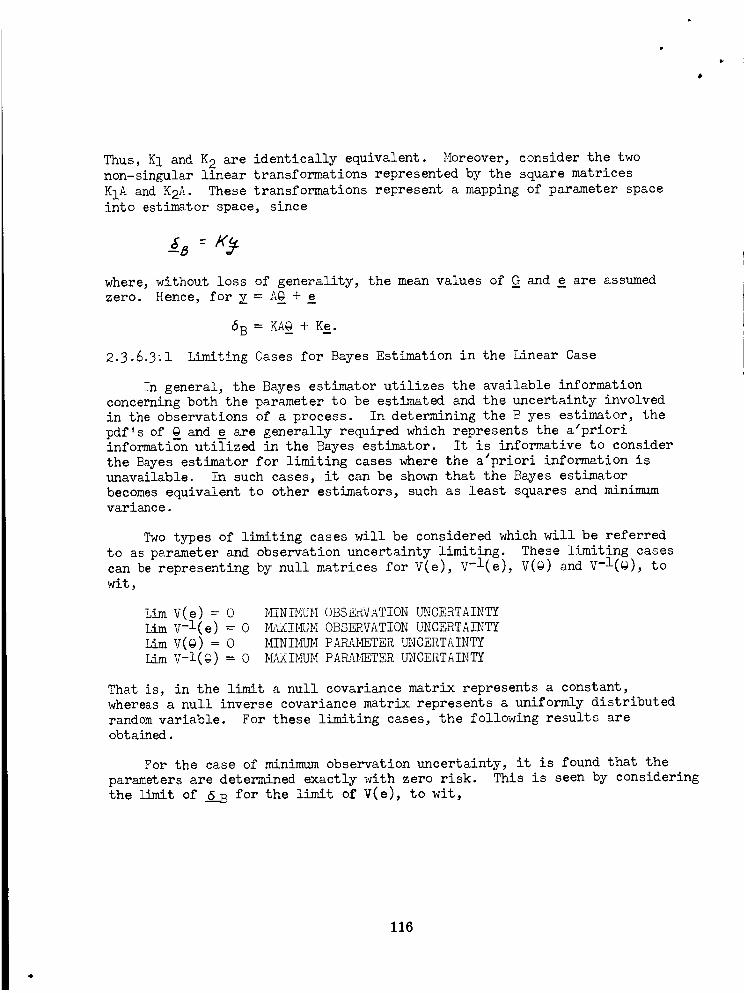
Thus, K1 and K2 are identically equivalent. Moreover, consider the two
non-singular linear transformations represented by the square matrices
KIA and K2A. These transformations represent a mapping of parameter space
into estimator space, since
where, without loss of generality, the mean values of _ and e are assumed
zero. Hence, for X = Am +
6B = KAY_+ Ke.
2.3.6.3_1 Limiting Cases for Bayes Estimation in the Linear Case
In general, the Bayes estimator utilizes the available information
concerning both the parameter to be estimated and the uncertainty involvedin the observations of a process. In determining the B yes estimator, the
pdf's of @ and e are generally required which represents the a'priori
information utilized in the Bayes estimator. It is informative to consider
the Bayes estimator for limiting cases where the a_priori information is
unavailable. In such cases, it can be shown that the Bayes estimator
becomes equivalent to other estimators, such as least squares and minimumvariance.
Two types of limiting cases will be considered which will be referred
to as parameter and observation uncertainty limiting. These limiting cases
can be representing by null matrices for V(e), v-l(e), V(@) and v-l(@), to
wit,
LimV(e) _ 0
Lim v-l(e) = 0
mim V(@) = 0mmv-l(_) = o
MiNI},IUM OBSE_{VATION UNCERTAINTY
_vZL<!MUM OBSERVATION UNCERTAINTY
MINI_,_,[ PAR&_.TER UNCERTAINTY
_6_IMUM PAPu&METER UNCERTAi%_TY
That is, in the limit a null covariance matrix represents a constant,
whereas a null inverse covariance matrix represents a uniformly distributed
random variable. For these limiting cases, the following results are
obtained.
For the case of minimum observation uncertainty, it is found that the
parameters are determined exactly with zero risk. This is seen by considering
the limit of iB for the limit of V(e), to wit,
116
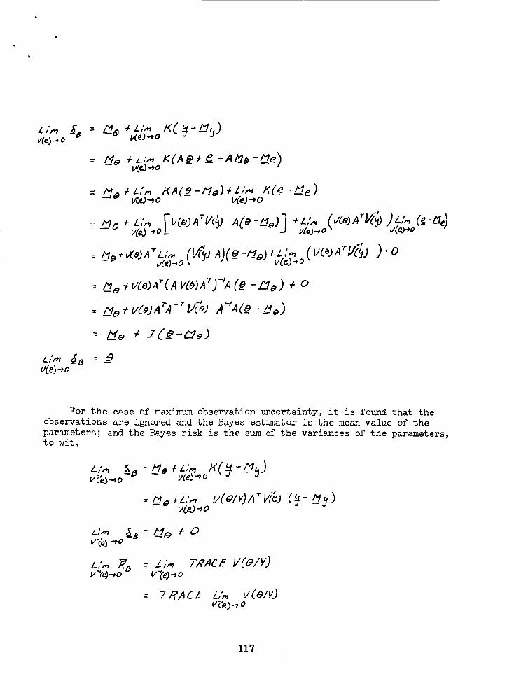
L /°frl
v(_) .-,o_B 4 L,',., K(_-L#_,)
_e) -_ o
_6, * L,'.., K(A __÷_ -A_ -Ge)v(eJ_o
= _/3e/ z,',. KA(e -_e) ,' z,'.,, _(_ -_Me)V_¢)-_O -- L/de.)_0 -
(_-_)V(_--,o I_ vd_.).-,o" "V(_-_o
vdeJ-_o - v(eJ-_o
- __o_Vde)A'(AV(_)A_)-'A(e-_) ÷ 0
= _Mo,'v(_JA",_-'Vi;,) _"A(_-_M,,)
= M_e ÷ Z(_e-_e)
vdeb-,o
For the case of maximum observation uncertainty, it is found that the
observations are ignored and the Bayes estimator is the mean value of the
parameters; and the Bayes risk is the sum of the variances of the parameters,to wit,
,;,,, _,_ = ,'.'z_,+z:,., /<(._ -_m_Jv C'_)--,o - v(eb "_o
=_ +L,',,v(#/V)A_V_J(_-__)
V'('_) 1-tO
- 7-RAC_ /,'_ v(e/v]vz'e)-_ o
llq
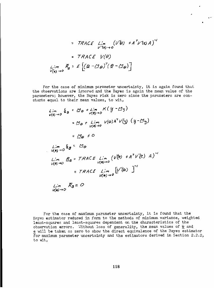
/_;m
: TRACE L,',. (L/'_2 /'Arl,,'-_debA.) -Iv-'_e)_ o
- 7,'?ACE V(e.)
For the case of minimum parameter uncertainty, it is again found that
the observations are ignored and the Bayes is again the mean value of the
parameters; however, the Bayes risk is zero since the parameters are con-
stants equal to their mean values, to wit,
/-"" _s = _ + z.,',,,,v(e) _ o J(e).._O
= _hie 7, L ;,,_v( eJaÜ
= -/'/o t. o
L ,',, _-o - _ e
L,',,_ R_ = TRII C E L,'_v(_e.).-*o _,(eg_o
: 7-R,qc -,,',,, Ev't'* ]-'
v(o) --,o
For the case of maximum parameter uncertainty, it is found that the
Bayes estimator reduced in form to the methods of minimum variance, weighted
least-squares and least-squares dependent on the characteristics of the
observation errors. Without loss of generality, the mean values of @_ and
e will be taken as zero to show the direct equivalence of the Bayes estimatorI
for maximum parameter uncertainty and the estimators derived in Section 2.2.2,
to wit,
118
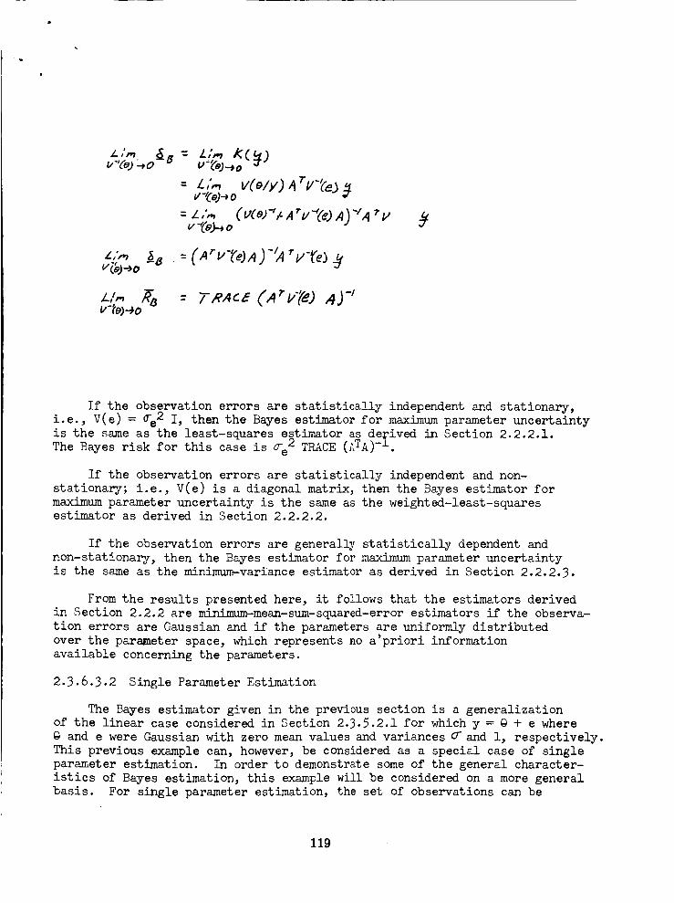
u " CeJ..+o "
= L;,., aTV'?e35V_Ee)-_0
= Z,',_ (V(e)_t.A'V_(e.)A'_'/A TVv "(e_ o
/_:,, - tRAcE (A"v 'J
If the observation errors are statistically independent and stationary,
i.e., V(e) = _e2 I, then the Bayes estimator for maximumparameter uncertainty
is the same as the least-squares estimator as derived in Section 2.2.2.1.The Bayes risk for this case is _e 2 TRACE (ATA) -1.
If the observation errors are statistically independent and non-
stationa_:; i.e., V(e) is a diagonal matrix, then the Bayes estimator for
maximum parameter uncertainty is the same as the weighted-least-squaresestimator as derived in Section 2.2.2.2.
If the observation errors are generally statistically dependent and
non-stationary, then the Bayes estimator for maximum parameter uncertainty
is the s_me as the minimum-variance estimator as derived in Section 2.2.2.3.
From the results presented here, it follows that the estimators derived
in Section 2.2.2 are minimum-mean-sum-squared-error estimators if the observa-
tion errors are Oaussian and if the parameters are uniformly distributed
over the parameter space, which represents no a'priori information
available concerning the parameters.
2.3.6.3.2 Single Parameter Estimation
The Bayes estimator given in the previous section is a generalization
of the linear case considered in Section 2.3.5.2.1 for which y = @ + e where
@ and e were Gaussian with zero mean values and variances _and l, respectively.
This previous example can, however, be considered as a special case of single
parameter estimation. In order to demonstrate some of the general character-
istics of Bayes estimation, this example will be considered on a more general
basis. For single parameter estimation, the set of observations can be
119
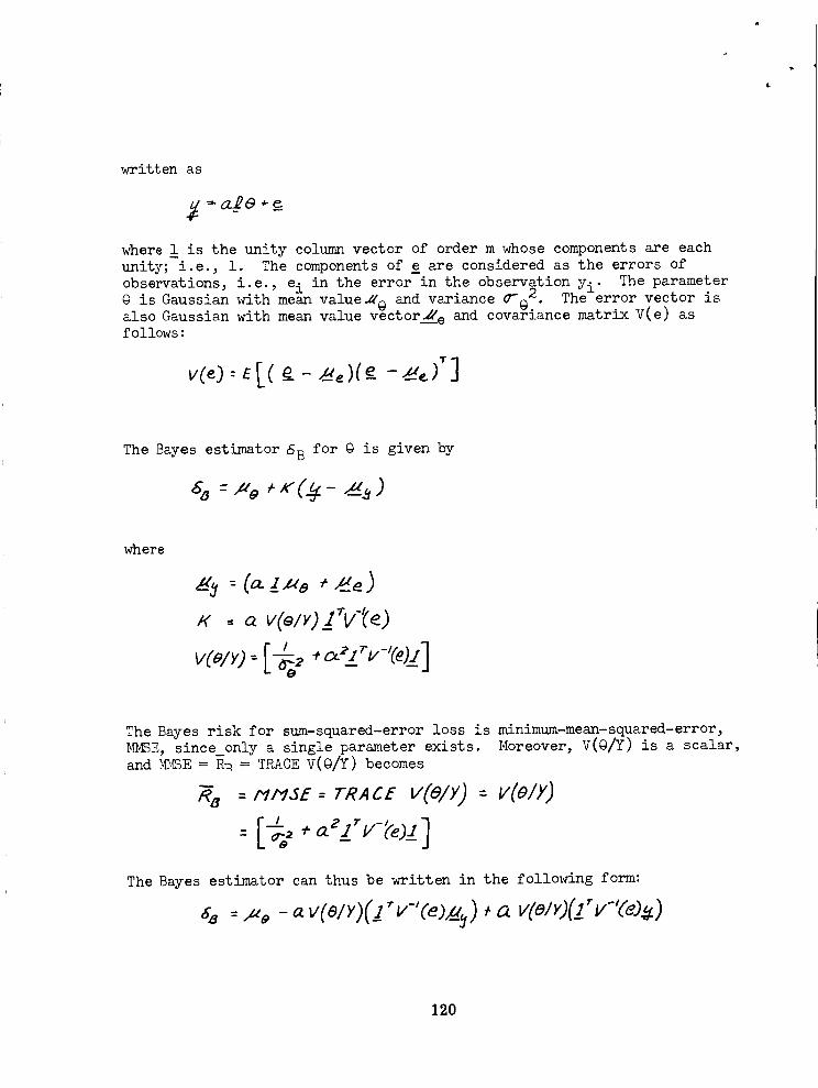
i
written as
where i is the unity column vector of order m whose components are each
unity; i.e., 1. The components of _ are considered as the errors of
observations, i.e., ei in the error in the observation Yi" The parameter@ is Gaussian with mean value JX_ and variance _ 2. The error vector is
also Gaussian with mean value v_ctor____e and cova_iance matrix V(e) asfollows:
v@): El( __- a,)fe_ - __,7]
The Bayes estimator 6 B for @ is given by
where
_z-<,_: (o__I/.<_,+_)
K -- _ V(elV)!_vt_)
The Bayes risk for sum-squared-error loss is minimum-mean-squared-error,
_SE, since_only a single parameter exists. Moreover, V(@/Y) is a scalar,
and _MSE = Ru = TRACE V(@/Y) becomes
_ : _M_E: TRACE v@l×) : v(_/y)
The Bayes estimator can thus be written in the following form:
68 : Ixe - a v(eiY)Cl" v"(e.)_ ) + cx vt@lYJ(j" v-'(eJ#)
120
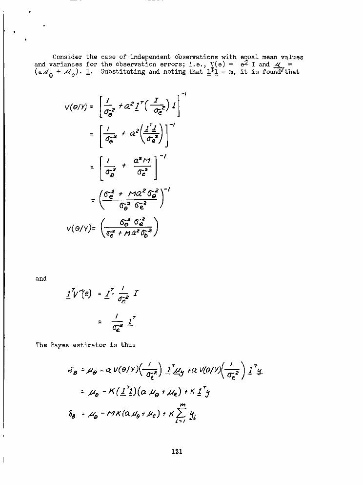
Consider the case of independent observations with e_ual mean valuesand variances for the observation errors; i.e., V(e) = ez I and 14 =
(a_@ +Me). _. Substituting and noting that I_T_ = m, it is fo_--dYdthat
v(_/d = 2 Tr .T _ ]-I-_//,'_ _1t-_j) x-/
v(ely)= (&, _2 _._÷ _a_ 2)
and
I
__'v't'eJ:/': _ z
The Bayes estimator is thus
: - _ _ ÷a v(ei !
% : ,uo -o_e(a/x_+l,,,)_ K.Z, t£%._.#
7
121
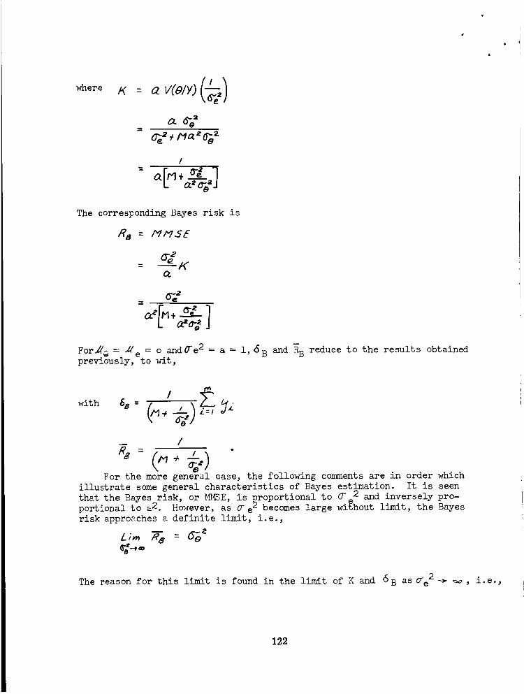
where
!
= aiM+ 7
The corresponding Bayes risk is
R 8 = M_VSE
ForY£@ = YJe = o andre 2 = a = i, _B and RB reduce to the results obtained
previously, to wit,
with
/
/
For the more general case, the following comments are in order which
illustrate some general characteristics of Bayes estimation. It is seen
that the Bayes risk, or _E, is _roportional to 6_e2 and inversely pro-portional to a2. However, as _ e becomes large without limit, the Bayes
risk approaches a definite limit, i.e.,
The reason for this limit is found in the limit of K and 6B aS_e 2-_ _, i.e.,
122
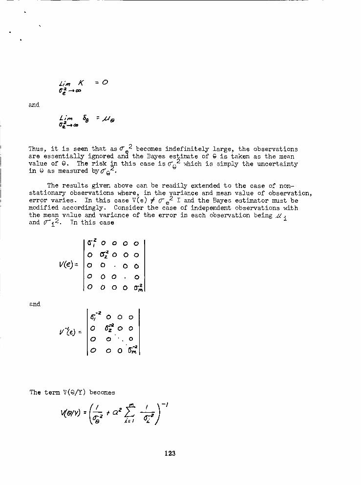
and
=0
L;,,, 58 =..U_
Thus, it is seen that as _2 becomes indefinitely large, the observations
are essentially ignored anS the Bayes estimate of @ is taken as the mean
value of @. The risk in this case is_@ 2 which is simply the uncertaintyin @ as measured bye@2.
The results given above can be readily extended to the case of non-
stationary observations where, in the variance and mean value of observation,
error varies. In this case V(e) _ O-e 2 I and the Bayes estimator must be
modified accordingly. Consider the case of independent observations with
the mean value and variance of the error in each observation being_ iand _--i2. In this case
_
• £ 0 o00
0 _0 00
0 0 0 0
0 00 0
0 O 0 0 O'_
and
o
0 o
0 00
The term V(@/Y) becomes
£= l .l
-!
123
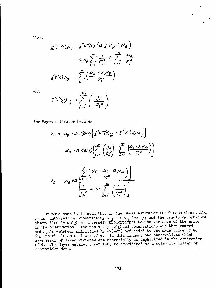
Also,
and
"( )
i" / (_
The Bayes estimator becomes
%.o c,. !_]
._ a _ I
In this case it is seen that in the Bayes estimator for @ each observation
Yi is "unbiased" by substracting _ i + ad_ from Yi and the resulting unbiasedobservation is weighted inversely proporti6nal to the variance of the error
in the observation. The unbiased, weighted observations are then summed
and again weighed, multiplied by aV(@/Y) and added to the mean value of @,
g/Q, to obtain an estimate of @. In this manner, the observations which
have error of large variance are essentially de-emphasized in the estimation
of @. The Bayes estimator can thus be considered as a selective filter ofobservation data.
124
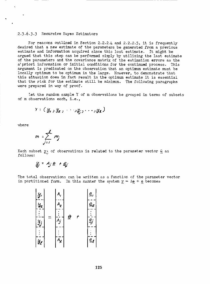
i
2.3.6.3.3 Recursive Bayes Estimators
For reasons outlined in Section 2.2.2.1 and 2.2.2.5, it is frequently
desired that a new estimate of the parameters be generated from a previous
estimate and information acquired since this lost estimate. It might be
argued that this step can be performed simply by utilizing the last estimate
of the parameters and the covariance matrix of the estimation errors as the
a'priori information or initial conditions for the continued process. This
argument is predicated on the observation that an optimum estimate must be
locally optimum to be optimum in the large. However_ to demonstrate that
this situation does in fact result in the optimum estimate it is essential
that the risk for the estimate still be minimum. The following paragraphs
were prepared in way of proof•
Let the random sample Y of m observations be grouped in terms of subsets
of m observations each, i.e.,
y:
where
j'=/
Each subset Zj of observations is related to the parameter vector @ asfollows:
The total observations can be written as a function of the parameter vector
in partitioned form. In this manner the system Z = A_ + _ becomes
..p,
m
A I
A_
eI
125
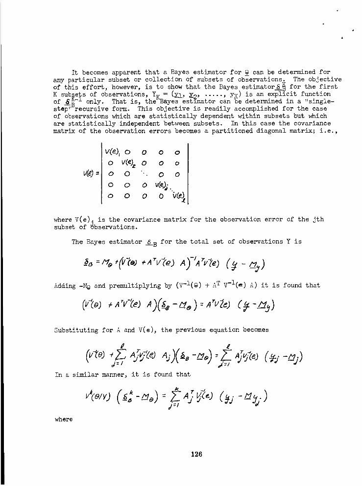
It becomes apparent that a Bayes estimator for @_ can be determined for
any particular subset or collection of subsets of observations. The objective
of this effort, however, is to show that the Bayes estimator _ _ for the first
K sub_e_s of observations, Yv = (El, Zo, ..... , y_) is an explicit function_--i • _ _ "" " " il "
of -_B only. That ms, the _ayes estLmator can be determlned mna slngle-step" recursive form. This objective is readily accomplished for the case
of observations which are statistically dependent within subsets but which
are statistically independent between subsets. In this case the covariance
matrix of the observation errors becomes a partitioned diagonal matrix; i.e.,
vCe),o o o oo v(% o o o0 0 '. 0 0
0 0 0 V(e),i"
o o 0 0 "{/(_..(
where V(e). is the covariance matrix for the observation error of the jth
subset of 6bservations.
The Bayes estimator _B for the total set of observations Y is
Adding -}_ and premultiplying by (v-L(@) + AT v-l(e) A) it is found that
Substituting for A and V(e), the previous equation becom.es
L
,,1=/
In a similar manner, it is found that
d:l
where
126
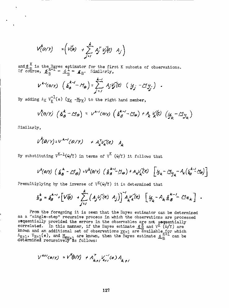
i
o_" /
and g K is the B_yes estimator
B-r-l= 6 _ = for the first K subsets of observations._rse,Of....6 B -_B" Similarly,
k-/
#'=1
By adding AK VKI(e) (YK -_K ) to the right hand member,
Similarly,
v"toid _v
By substituting vK-I(@/Y) in terms of V K (@/Y) it follows that
Premultiplying by the inverse of vK(@/Y) it is determined that
k k-i [ °_ )1:& +V" "_ +J:!
From the foregoing it is seen that the Bayes estimator can be determined
as a "single-step. recursive process in which the observations are processed
sequentially provided the errors in the observables are not sequentially
correlated. In this manner, if the Bayes estimate g_g_Kand VK (@/Y) areknown and an additional set of observations XK+l are available for which
A_, Va_(e), and __vJM-_ are known., then the Bayes estimate 8 K+I can be
determined recursive_t_s follows: _---B
12'7
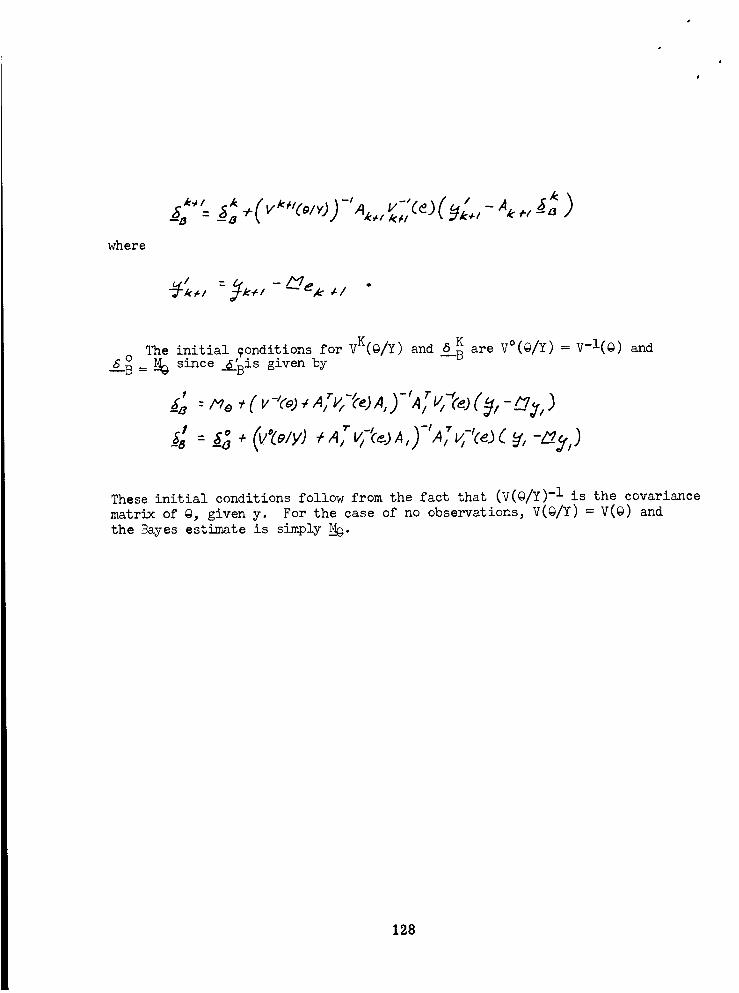
J
where
#_,.+, _+, - _. +,, .
g____=_ since 8__'Bisgiven by
The initial 9onditions for vK(@/Y) and S___ are V°(O/Y) = v-l(o) and
These initial conditions follow from the fact that (V(@/Y) -1 is the covariance
matrix of @, given y. For the case of no observations, V(@/Y) = V(@) and
the Bayes estimate is simply _:_.
128
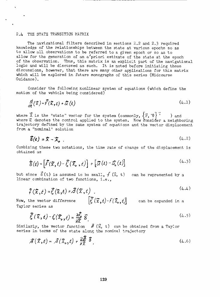
2.& THE STATE TRANSITION MATRIX
The navigational filters described in sections 2.2 and 2.3 required
knowledge of the relationships between the state at various epochs so as
to allow all observations to be referred to a given epoch or so as to
allow for the generation of an alpriori estimate of the state at the epoch
of the observation. Thus, this matrix is an explicit part of the navigational
logic and will be discussed as such. It is noted before initiating these
discussions, however, that there are many other applications for this matrix
which will be explored in future monographs of this series (MidcourseGuidance).
Consider the following nonlinear system of equations (which define the
motion of the vehicle being considered)
where _ is the "state" vector for the system (commonly, {F,-_} T ) andwhere _ denotes the control applied to the system. Now _onsiaer a neighboring
trajectory defined by the same system of equations and the vector displacementfrom a "nominal" solution
_(_) - - (_.2)= _ -.7.. o .
Combining these two notations, the time rate of change of the displacement isobtained as
but since _(t) is assumed to be small, _ (_, t)
linear combination of two functions, i.e.,
(_.3)
can be represented by a
Now, the vector difference [_o ('_,;_)-f'(<,_)] can be expanded in a
Taylor series as
=Similarly, the vector function B (_, t) can be obtained from a Taylor
series in terms of the state along the nominal trajectory
= 88X .
129
Thus, the differential equations for the system become
- A(_)_+ f(_J,
(h.7a)
(A.7b)
But, the trajectory for the motion under consideration itself isexpressible (analytically and/or numerically) as a unique function of the
position and velocity at some epoch, and as a function of the accelerations
experienced relative to a nominal path (differences in the gravitational
accelerations and in any applied thrusts). This set of relationships is
represented by
r = ro _3r_, r.+_ ,BI_
Thus, by a Taylor's expansion
and
(_.9)
_ _ _ _ _ T( )" --: _ . C 8_ (_.io)r:r_ + _-_ _r_ + _
where _( S_ ) is a set of linear functions which additively (due to thesmall assumed magnitude of the deviations) represent the effects of the
differences in the perturbing forces, and where B and C are 3 x 6 matrices.
These linear equations can, in turn, be expressed as
(_. lla )
(h.llb)
130

showing that, to the first order, the dynamics of the problem can be repre-
sented by the two matrices _ (t, t o ) and _ (t, to).
Now, comparing the two equations for 8and _-equations (&.7) and
(&.ll)_/, it becomes apparent that the fundamental solution matrix _-the
state transition matrix, the matrix denoted by @9 (t, to)_7 is the solutionto the homogeneous equation obtained for # = O. In order to define the
nature of the term _ (t,_t o) _ (6_) it is, however, necessary toconsider the solution to 8 (t).
Let _ (t) denote the homogeneous part of the solution for _ (t).
Then
But
Thus,
(_.12)
At this point, introduce the system of differential equations adjoint to
this family
(_.13)
and note that
d
Performing the substitution yields
(z_.z4)
131
which, upon integration, can be written as
t÷f x( dr_o
t°
(4.15a)
(4.15b)
-i
Multiplying by J__ (t, to) now reduces this result to
4 t
_o
(4.16)
Finally, comparing_the form of this equation to that given earlier
_-equation (_.iI)_/ for _ (t), it is apparent that
and that
(4.i7)
(4.is)
The preceding material clearly establishes the mathematical nature of
the state transition matrix and, at the same time, introduces the adjoint
equations as one means which might be employed to compute this matrix. The
sections which follow will explore these avenues in some detail for the
purpose of providing the state transition matrix as required in the naviga-tional filter.
132
2.4.1 Generating The State Transition Matrix
2.4.1.1 By Direct Integration
The introductory paragraphs to this section of the report showed that
the state transition matrix obeys the differential equation (4.12)
and the boundary conditions
-z
Thus, the desired matrix can be obtained directly by numerical integration of
each element of the array. This procedure is completely adequate for most
applications in which the task is concerned only with the reduction of
observed sightings (fixed values of to).
However, there are applications (midcourse corrections, for example) in
which the state transition matrix relating the state of the present epoch
and a fixed future epoch (e.g., the epoch of rendezvous) is desired. For
these applications, it is unnecessarily complex to require that the preceding
integration be reperformed at each epoch (i.e., a new to at each epoch).
Rather, it is convenient to generate the desired solutions as follows:
(r) - ¢,{T,t.,) (4.19b)
Thus,
(0: to) ).This technique requires that two integrations and an inversion be accomplished.
First, the transition matrix Eelating the arbitrary epoch (to) and the fixed
end time (T) is _enerated. L This integration need be performed only once,providing that g (t) never leaves the neighborhood of the nominal trajectory
about which the partials are evaluated.__ Secondly, the transition matrix
relating the arbitrary epoch (to ) and the epoch of the present state must begenerated from the previous transition matrix, the differential equation, and
the change in the time. Finally, the latter matrix must be inverted.
The first two of the three steps outlined are relatively simple. However,
the third involves a considerable amount of effort if normal matrix inversion
techniques are employed. Thus, it is instructive to present a means of
developing the inverse in an analytic manner from the transition matrix
itself. This procedure, if employed, will avoid roundoff and loss of
significance problems inherent in numerical techniques, in addition to
133
drastically simplifying the mechanization logic.
Consider a linear system (expressed in cartesian coordinates) described
by the following equation
2 :A(:_) i(,O (&._l)
where 6 (t) is an even-ordered state vector composed of a set of output
variables and their derivatives; and A(t) is a coefficient array for the
system composed of square, symmetric, even-ordered subarrays of the followingform
[4,-Io]This form for A(t) is representative of motion in conservative force fields.
To be specific
A#Z =I
r 2 ]for motion in the vicinity of
(&. 22b )
(_.2#c)
If equations (1..22) and (1..23
following identity results
J, ]
are substituted back into equation (l,.21), the
and upon expansion, equation ( " ) .yields
_,z : Wzz
%z,: __L_,,_r
9F
(1..25a)
(A.25b)
(&.25c)
(&.25d)
134
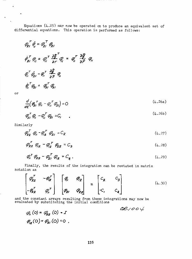
Equations (&.25) may now be operated on to produce an equivalent set of
differential equations. This operation is performed as follows:
a_
• T rg #_,= g, g,
or
d r T
a7(_,,#,,-_,,_0 -or
(&.26a)
(/_.26b )
Similarly
#,_¢,,-#,2_, =c_ (/_. 27)
Finally, the results of the integration can be restated in matrixnotation as
T
i i<-_Z _'J L#,, ¢_] , qand the constant arrays resulting from these integrations may now beevaluated by substituting the initial conditions
_,,(o; = _, (o) - z
(z_.30)
_,, Co) - #_,(o) =o.
135
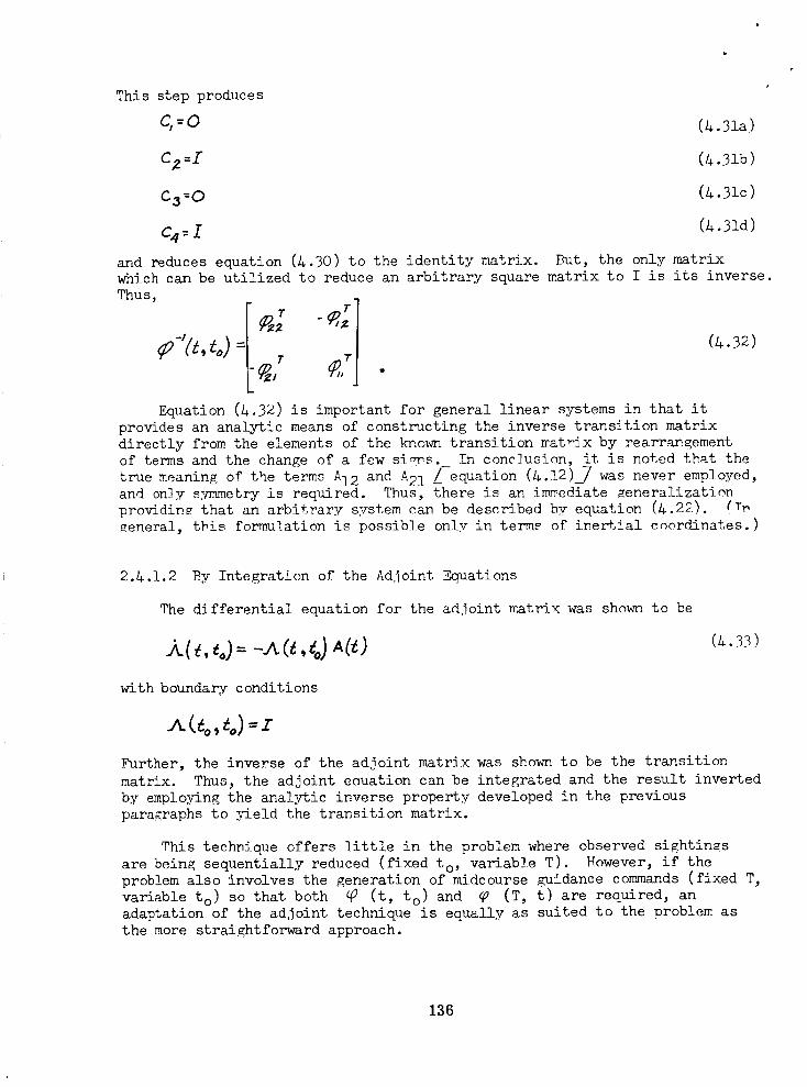
This step produces
C, -- 0 (_ .31a.)
cz=I (4.31b)
C3= 0 (4.31c)
c4=f (4.31d)
and reduces equation (4.30) to the identity matrix. But, the only matrixwhich can be utilized to reduce an arbitrary square matrix to I is its inverse.
Thus, .,
= c/*.32)
Equation (/,.32) is important for general linear systems in that itprovides an analytic means of constructing the inverse transition matrix
directly from the elements of the known transition mat,_x by rearrangementof terms and the change of a few simms. In conclusion, it is noted that the
true meaning of the terms A12 and A21 _/-equation (/*..'12)_ was never employed,and only s,_nnmetry is required. Thus, there is an immediate _eneralization
providin_ that an arbitrary system can be described bv equation (4.22). (rr
_eneral, this formulation is possible only in terms of inertial coordinates.)
2._.I.2 By Integration of the Adjoint Equations
The differential equation for the adjoint matrix was shown to be
with boundary conditions
(/*.33)
Further, the inverse of the adjoint matrix was shown to be the transition
matrix. Thus, the adjoint enuation can be integrated and the result inverted
by employing the analytic inverse property developed in the previous
paragraphs to }_eld the transition matrix.
This techDique offers little in the problem where observed sightin_s
are bein_ sequentially reduced (fixed to, variable T). However, if the
problem also involves the generation of midcourse _uidance commands (fixed T,
variable t o) so that both @ (t, to ) and _ (T, t) are required, an
adaptation of the adjoint technique is equally as suited to the problem as
the more straightforward approach.
136
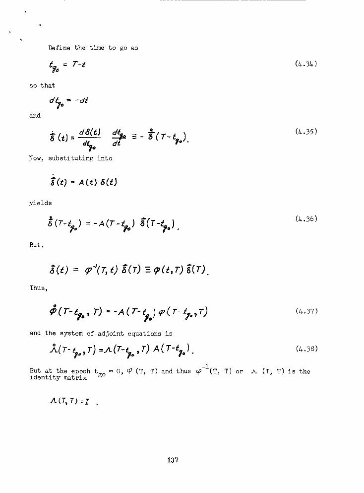
so that
and
Define the time to go as
= y'-_
d_lo = -d_
Now, substituting into
But,
Thus,
= -A(T-
$(r-_o, r) =-A(r- _,o)_(r _I.,T)
and the system of adjoint equations is
A(r-_., r) : _(r-_r.,r) A(T-_.)
But at the epoch = 0 @ (T, T) and thusidentity matrix tg° '
.A.(T, T) :Z
@-I(T, T) or (T,
(_.35)
(L.36)
(a.37)
(_..38)
T) is the
13'7
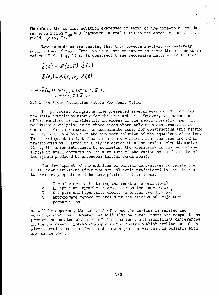
Therefore, the adjoint equation expressed in terms of the t_me-to-_o can be
integrated from t _ -- O (backward in real time) to the epoch in question to
yield _ (t, T). _U
Note is made before leaving that this process involves successively
small values of t_o. Thus, it is either necessary to store these successive
values of _- (ti, T) or to construct these successive matrices as follows:
Thus, _£Z) : _(_. _ _ ) _(_, T) gCT)
2.A.2 The State Transition Matrix For Conic Notion
The precedin_ paragraphs have presented several means of determinin_
the state transition matrix for the true motion. However, the amount of
effort required is considerably in excess of the amount normally spent in
preliminary analysis, or in those cases where only moderate precision is
desired. For this reason, an approximate lo_ic for constructing this matrix
will be developed based on the two-body solution of the equations of motion.
This development is justified since the deviations from the true and conic
trajectories will agree to a higher de_ree than the trajectories themselves
(i.e., the error introduced by neglecting the variations in the perturbi_
forces is small compared to the ma_itude of the variation in the state of
the system produced by erroneous initial conditions).
The development of the matrices of partial derivatives to relate the
first order variations (from the nominal conic trajectory) in the state at
two arbitrary epochs will be accomplished in four steps:
i.
2.
3.
Circular orbits (rotating and inertial coordinates)
Elliptic and hyperbolic orbits (rotatin_ coordinates)
Elliptic and hyperbolic orbits (inertial coordinates)
Approximate method of inc!udin_ the effects of trajectory
perturbation
As will be apparent, the material of these discussions is related and
sometimes overlaps. However, as will also be noted, there are computational
problems associated with some of the functions, and significant differences
in the coordinate systems employed in the analyseswhich combine to suit a
given formulation to a given task to a higher degree than is possible with
any single step.
138
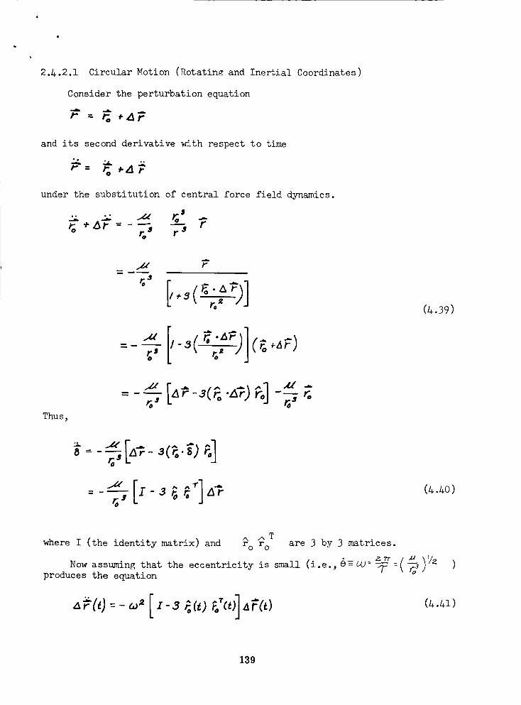
2.1.2.1 Circular Motion (Rotatine and Inertial Coordinates)
Consider the perturbation equation
/" = r. ÷_r
and its second derivative with respect to time
under the substitution of central force field dynamics.
.. ._ ._, _s .,..+A = r"s rS r
Thus,
r
_J ros r_
(_.39)
GS(_.&o)
_ ATwhere I (the identity matrix) and ro ro are 3 by 3 matrices.
Now assuming that the eccentricity is small (i.e., 0-_U: -_ :produces the equation
(A._l)
139
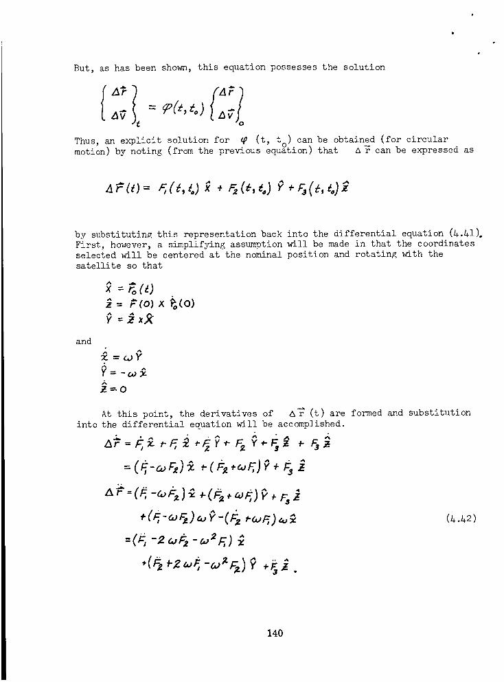
But, as has been shown, this equation possesses the solution
Thus, an explicit solution for _ (t, t ) can be obtained (for circular
motion) by noting (from the previous equation) that A ? can be expressed as
by substitutin_ this representation back into the differential equation (&.hl)o
First, however, a simplifying assumption will be made in that the coordinates
selected will be centered at the nominal position and rotating with the
satellite so that
,_ -- ro(_-)= F,,o)x %(o)
and
fAY- -_:£
_.---0
At this point, the derivatives of
into the differential equation will be accomplished.
• _% 4%
A r (t) are formed and substitution
(h.h2)
140
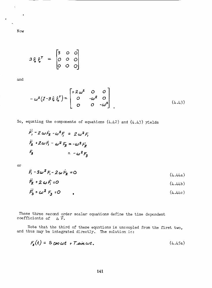
N oN
-- O
O
and
o o]0 0 -W ,
So_ equating the components of equations (/+./4.2)and (_._3) yields
_2_#, - _,__ --_
or
#, -3u2 F,- 2.o_& =0B)
& +z #,.,F;=o
+o,__ :o . (4.&&c)
These three second order scalar equations define the time dependentcoefficients of _ r.
Note that the third of these equations is uncoupled from the first two,and thus may be integrated directly. The solution is:
(a.aSa)
141
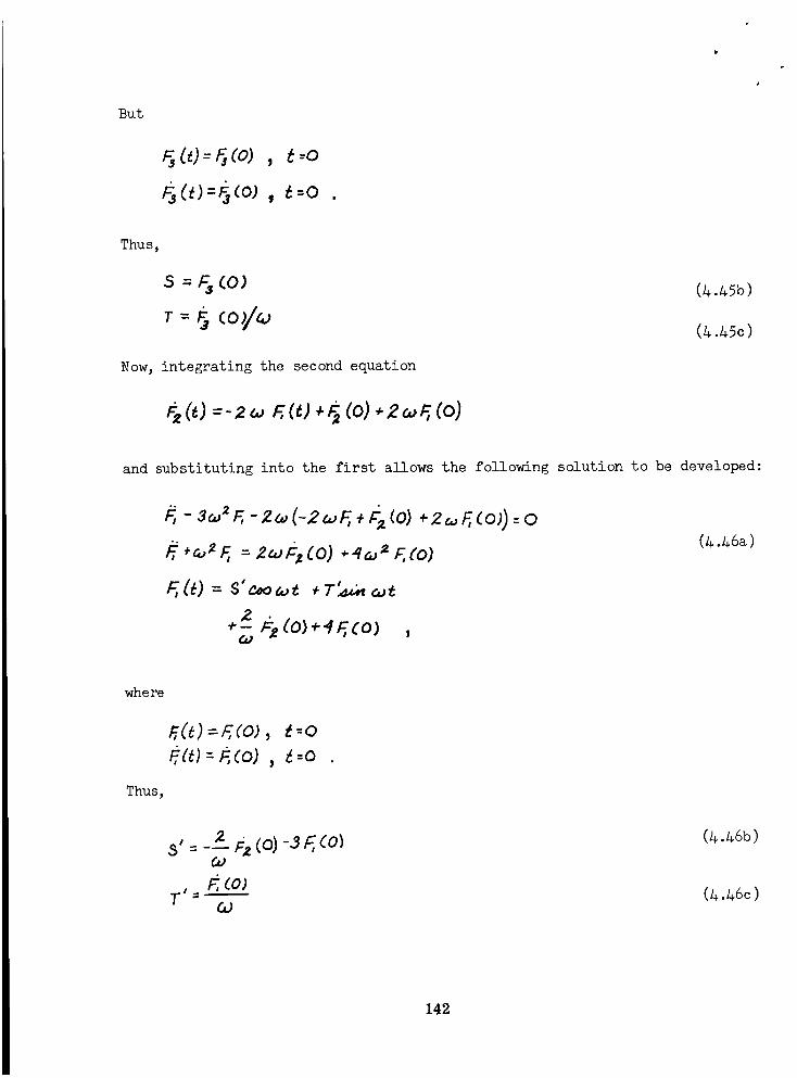
But
Thu s,
Now,
s = F, (o_
integrating the second equation
_(d=-2,.,., ;,(_),#,(o)÷z_q(o)
and substituting into the first allows the following solution
_,-s_F,-Z_(-2_F,÷&(o)+2_F,(o)):O
F, ,J F, = Z_,_, CO)._2 F,(o)
,- Fz(O)÷4F,(O) ,(4)
where
Thus,
fi(t) =F,(o),_;o
s' = -_--F2(o)-sF,(o)_)
F;(o)CO
to be developed:
(&.&6a)
(&.L6b)
(&.&6c)
142
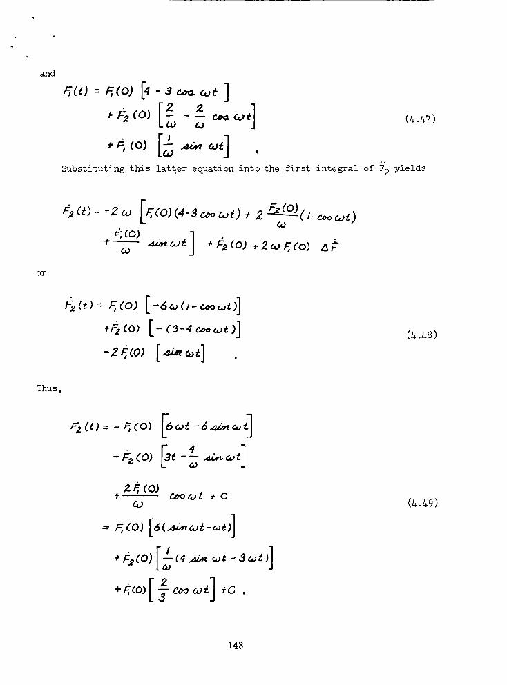
and
this latter equation into the first integral of F'_Substituting yields
(_._7)
or
k¢o) ](.4.)
+_(o) ,2_F,(o) a#
-2;;(o)[_,] .(4.&8)
Thus,
,m_('_)=-F,,('O) [602_ -6495_(_£]
z_,co_60
= P,, ( O ) [ 6 ( AL,,, co _ - (o _ )]
(z,.._9)
143
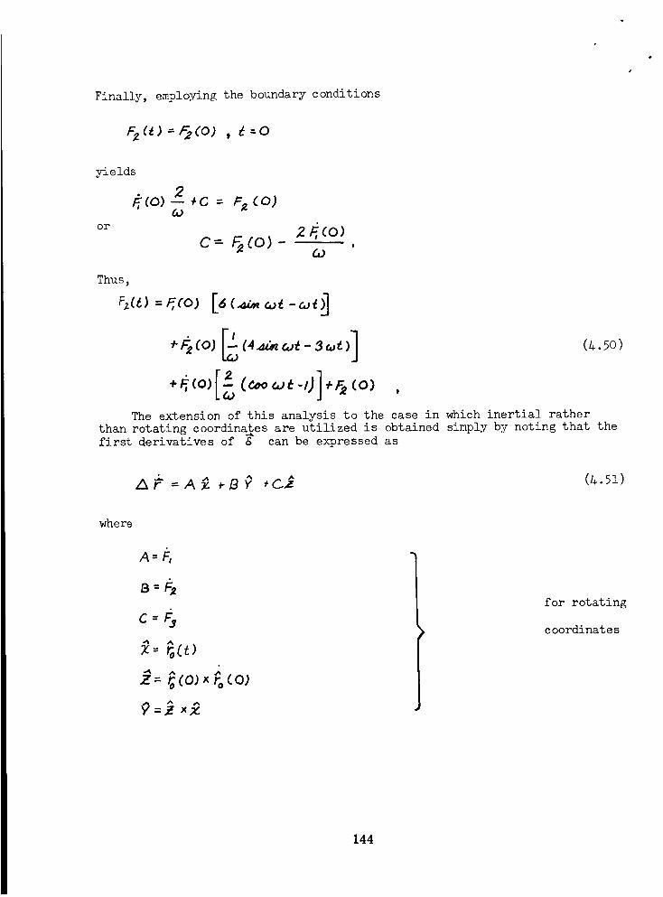
Finally, employing the boundary conditions
F2(_)-=_(O) , _=o
yields
g(o) Z ÷c = r 2 _o)(._
or
c- _co)-2_(o)
CO
Thu s,
The extension of this analysis to the case in which inertial rather
than rotating coordinates are utilized is obtained simply by noting that the.-L
first derivatives of 6 can be expressed as
(&.5o)
where
A=_
s=&
c=#sfor rotating
coordinates
144
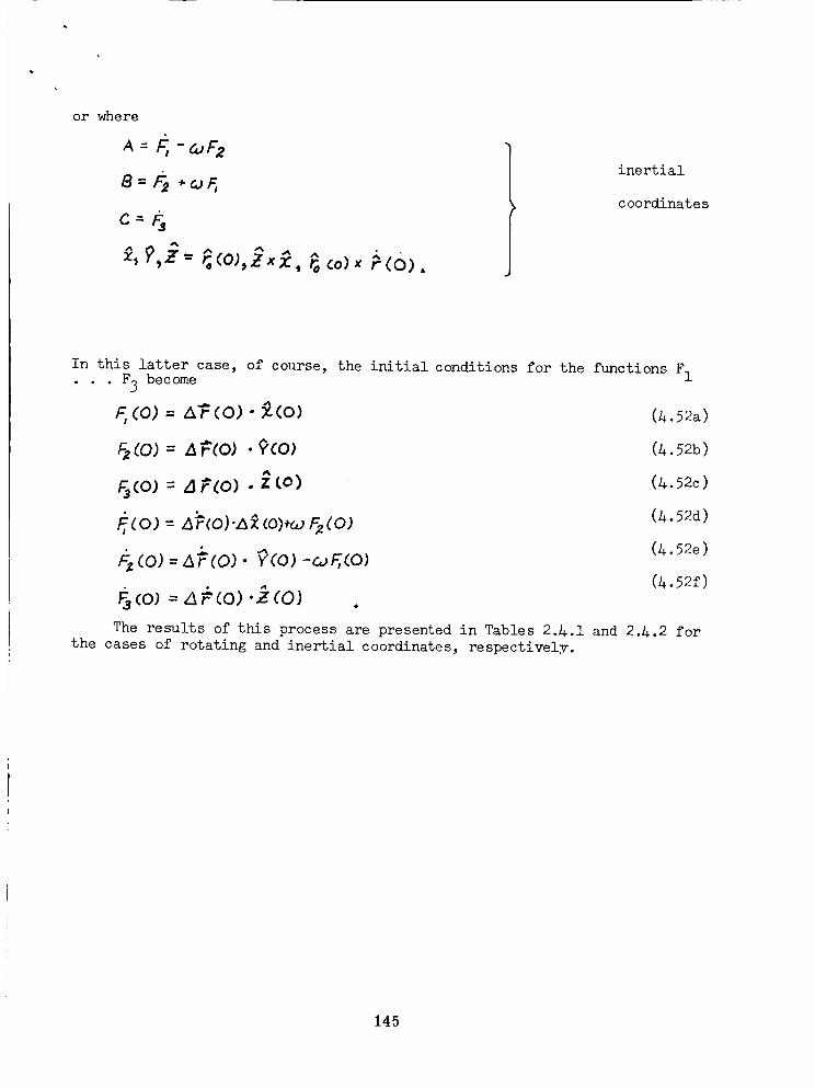
b
or where
A- #,-_,F2
A_,P,_- _co),_, _ _o)x_-(0_.
inertial
coordinates
In this latter case, of course, the initial conditions for the functions FI• F3 become
_('o) : a_co) • _.(o)
&co) =af(o)-?co) -_F, CO)
#s_o_=nkco) .#(o) .
(h.52a)
(h.52b)
(4.52c)
(h.52d)
(_.52e)
(_.52f)
The results of this process are presented in Tables 2._.I and 2.h.2 for
the cases of rotating and inertial coordinates, respectively.
145
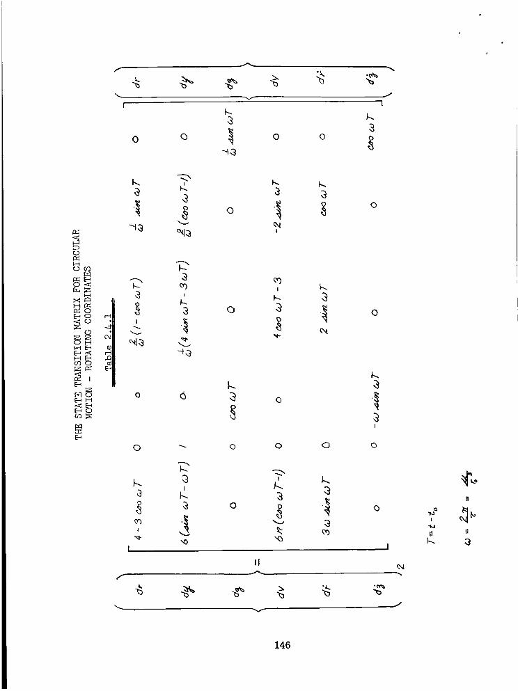
_D
H000
O
r_
I
E--_H
[--_O_N
f
I
J
I
0 O
}-.
0 o
o
e,l!
O
I
o
I
1
I
6
-2"
I
"0
O
g.
O
O
I
F-.
o
O
!
e,i
o
k
o
I
O
0
f
11A
J
146
0
!
11
II
II
#
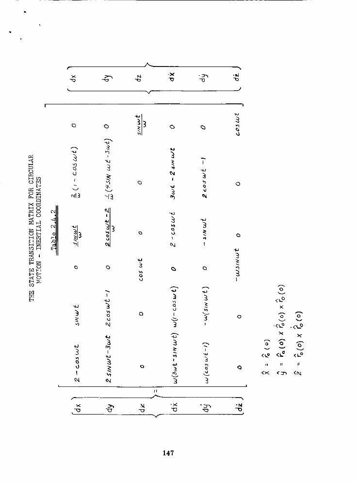
o
HcO
E_
o_E,H
E--_O
H
I---4
_Zo
_ H
x _ _ .x ._-_
_J
I
-..-t
3
E-_
4--;
0O
I
!
f-
V
!
0
i"
v_o_J
n_I
_J
_J
0
43
!
r5
0
,JI
tx_
0
o
I
;
I
'o
t_
I!
I
3!
I
,,%
0
,q
I
0
0
x
Ao
<0 <ff <L°
II II II
<x <=7-_ <_
147
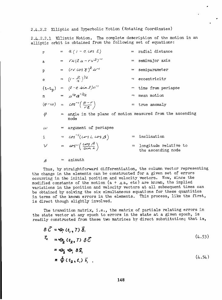
2.4.2.2 Elliptic and Hyperbolic Motion (Rotating Coordinates)
2._.2.2.1 Elliotic Motion. The complete description of the motion in an
elliptic orbit is obtained from the following set of equations:
r = _ (I - _ca_ E) = radial distance
a = F_ (2 _ - rV2) -_ = semimajor axis
p = (rv(x._)zzl -I = semiparameter
e = (i_ _)_z = eccentricity
(t-tp) = (£-g_£9_ -I = time from periapse
n = _-31a = mean motion
(@-cu) = gz_-' ( p - r)_- = true anomaly
= angle in the plane of motion measured from the ascendingnode
= argument of periapse
-i )i = _ (_L_u_ = inclination
( c_/_ ) = longitude relative tol) = _-' _ the ascending node
= azimuth
Thus, by straightforward differentiation, the column vector representing
the change in the elements can be constructed for a given set of errors
occurring in the initial position and velocity vectors. Now, since the
modified constants of the motion (a + Aa, etc) are known, the implied
variations in the position and velocity vectors at all subsequent times can
be obtained by solving the six simultaneous equations for these quantities
in terms of the known errors in the elements. This process, like the first,
is direct though slightly involved.
The transition matrix, i.e., the matrix of partials relating errors in
the state vector at any epoch to errors in the state at a given epoch, is
readily constructed from these two matrices by direct substitution; that is,
.ib
8C
(_.$_)
148
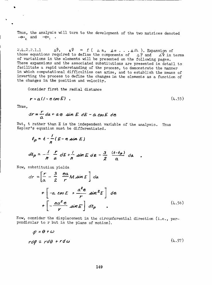
Thus, the analysis will turn to the development of the two matrices denoted
_e_ z and _
2._.2.2.1.1 a_, a_ = f ( a aj Ae . . A/h ). Expansion ofthose equations required to define the components of &_ and Av in terms
of variations in the elements will be presented on the following pages.These expansions and the associated substitutions are presented in detail tofacilitate a rapid understanding of the process, to demonstrate the manner
in which computational difficulties can arise, and to establish the means ofinverting the process to define the changes in the elements as a function ofthe changes in the position and velocity.
Consider first the radial distance
r---aU-ec,_) .
Thus,
rdr = -- da + a e _£,,zE d£ - _ @ F- de
But, t rather than E is the independent variable of the analysis.Kepler's equation must be differentiated.
n
Thus
/ ,3 C_-Ep) d_d_p = I r dE *-- _,z F_ d P_ - --a n 2. a
Now, substitution yields
dr = -_ r
GtZe ]_- -a. _ E ,-- ,,_z4Z E de
r
÷[ _16c2--e_zl'zEJr d_p .
(_.56)
Now, consider the displacement in the circumferential direction (i.e., per-
pendicular to r but in the plane of motion).
(_. 57 )
149
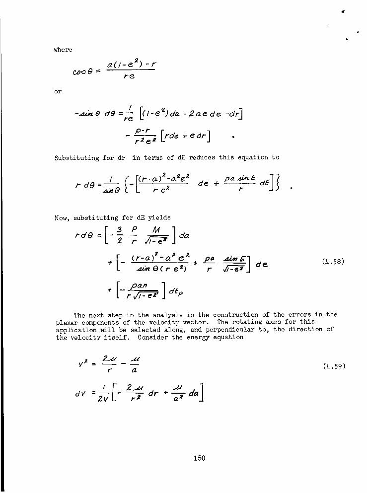
where
a(/-_ 2) -r
r_
or
/ r
-.aOz _ d9 = I('-- /_e 2)re L.
da -2 a e de -dr]
r2_a de r ¢dr
Substituting for dr in terms of dE reduces this equation to
r ae f-L 7 p E E]Ide +
,r
Now, substituting for dE yields
d_
÷[- (r-a)_-a_e__O(re 2) + P-_r _]
pa_
d_ (#._8)
The next step in the analysis is the construction of the errors in the
planar components of the velocity vector. The rotating axes for this
application will be selected along, and perpendicular to, the direction of
the velocity itself. Consider the energy equation
V _ -- __ --__
F
dV = -- - a22V r2' dr * -- da
(_.59)
150
substituting for dr
r a a t -2 r -_
_._x 2._x aZe _xS,_EI de
2.z.z /l a 2 e _xz g ] dip+-;;-7-
or
V J .zz oc ]dv = -_-- + emma d_
Za X r_v r
+ -- en_ d6pr
Finally, consideration of the angular momentum will provide the infor-
mation necessary to construct the variation in the velocity perpendicularto the nominal direction
rZv _ Cmo2 y =._a(I-e _)
2 _z___# 2_pdr + dv - 2_p_v_ _ d _" (A.61)
r V
2_xzp [ (l-eZ) ae ]Z p da - --p de
so that
V r dr dv
vd_" =_ [ +r F v -- de -P
151
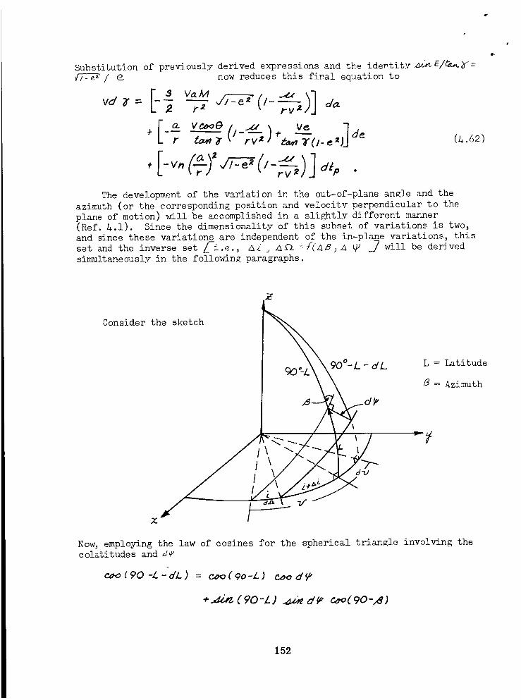
Substitution of previously derived expressions and the identity _,_E/ta._'=/ _ now reduces this final equation to
vd_'= -- -- _ I-_ da2 r a rv ;_
[ ,J+ .... der "_ _r rv • (A .62)
The development of the variation in the out-of-plane angle and the
azimuth (or the corresponding position and velocity perpendicular to the
plane of motion) will be accomplished in a slightly different manner(Ref. &.l). Since the dimensionality of this subset of variations is two,
and since these variations are independent of the in-plane variations, this
set and the inverse set _-i.e., _L j _fl =l(aB j _ _ _7 will be derived
simultaneously in the followin_ paragraphs.
¢
Consider the sketch
90°-L - dL L = Latitude
= Azimuth
/ \\II/
Now, employing the law of cosines for the spherical triangle involving thecolatitudes and d_
_ ( 90 -L -dL ) = cao ( qo-L ) cao d _"
+.d.d._ (90-/.) ._ d_ e.aoC90-_)
152
which is approximately
or
.a/_ L _" c_oL d L = ,_ L - eeo L .,uZ,_X_ d lt,
d/..= - -,_,_ ._d_. (_.63)
But, from spherical trigonometry
e.o<,Z = _ao/...,_ .,d
so that
d,,_ - dp,
(&.6_)
The error in the node (dx_) is obtained by considering the projection
of the erroneous trajectory on the reference plane, i.e.
_(7/' +dz) -d.a) -"_(/s ,d,_) (L_.65)
.,_._(i,di)
which is approximately
or
But
ea_ 7.)- _ _)(d z)- d _ ) =
z# (dz)-do.)-
_ / + e..aoL dZ
¢e,,_o,,_-.,_,_.,_d,a)(/_e_MZdZ)
..ax.J_(d zs) =_x_ ( 90 +/3 )
(90-L -AL )
d,8 7" dg
d_
153
so
_x9----- d#._L (k.66)
Thus,
do.= d,d - dz" -/"
or
These variations can be written in the form
L _'2, a22J
e_Ld_
(&.67)
(&.6s)
Thus, solving for the column vector (d_ , d_ ) is possible by computingthe inverse matrix
A-,.ra,, -_,,] --
L-_21 _,, J /AI
The results of this process are
.[- _,_(_ '_, '___)1_t _L ,J
dz.:
(6.69)
and
These results are summarized in Table 2.i.3.
(_.7o)
154
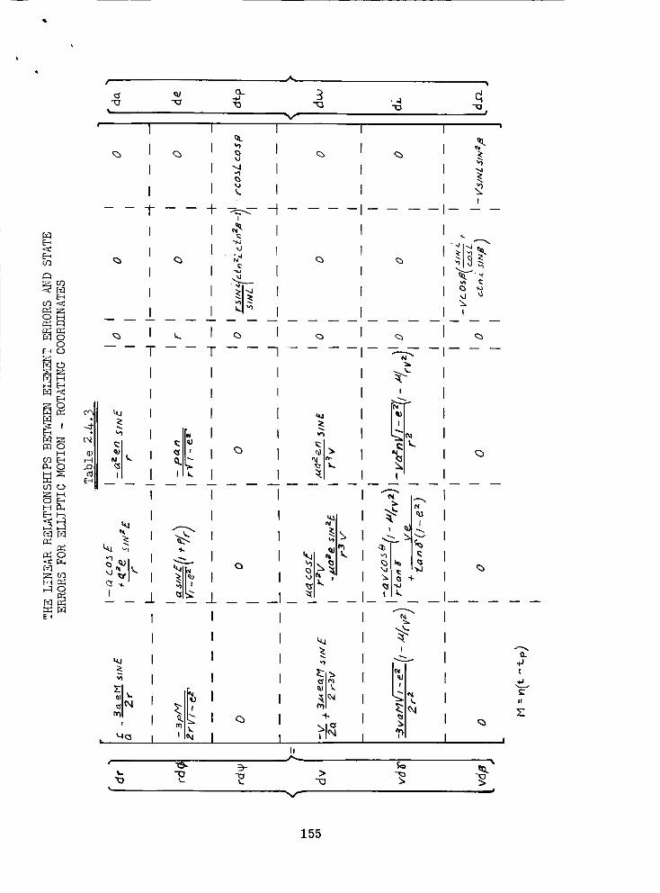
E_
_Z0
00
E-I r.._
HE-g
E-,
_2
_ozI-4
o"1 r_._
Hf:k,E--4H
_--_O
E-t
4..c',l
_5
u.l
I
u_
| t.l i:_
I
I
I
I
-1-
I
I
I
I
I
_1
I
I
I
I
I
I
I
_5
.'gC'-'N
I
I
I
I
-t-
I
I
I
I
I
%
t/"-4
%
!
_1.•
_5
I
I
I
I
Y
II
v
3
_5
_5
,,_. '
% I_
_1_/_
!
i
I
I
I _I
I
I
I
I
_E
155
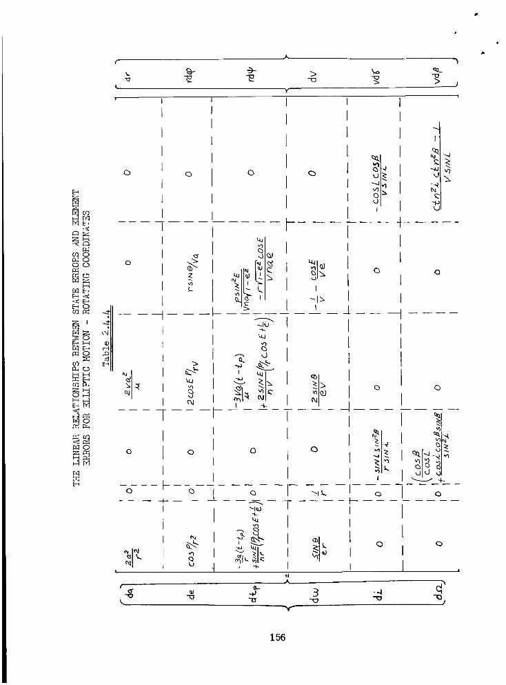
r:_ E-,
0"_0_0O0
H
,_E-_E-_O
_, 4
cer._
_0
m
-_ -g j
0
o
0
0
0
-4-I
IIII
2_
t'N
(b
(b
k)
0
t.tj
I q-
0
I
I
q)
"1 k.
'4--.
I
C)
I
0
I
I
I "d
---d
tO
0
0
I%-4I
I aa
IIII
\
113
i!
-_ 3 "_!
156
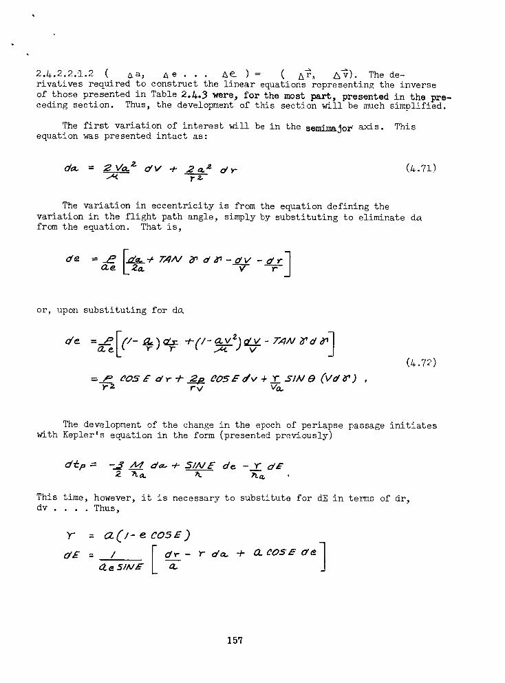
2.&.2.2._.2 ( Aa, Ae • • Ae ) = ( A_, _). The de-rivatives required to construct the linear equations representing the inverseof those presented in Table 2._.3 were, for the most part, presented in the pre-ceding section. Thus, the developmentof this section will be muchsimplified.
The first variation of interest will be in the semimajor axis. Thisequation waspresented intact as:
The variation in eccentricity is from the equation defining thevariation in the flight path angle, simply by substituting to eliminate dafrom the equation. That is,
or, upon substituting for do.
--- P O05E dr-l'_g C05Edv÷ ____5/A18 (VdY)-F'z r v v_.
(& .72)
The development of the change in the epoch of periapse passage initiates
with Kepler's equation in the form (presented previously)
d@p - -3 /Vl d_../- 51AIE de - Y" dE
,2 "a.o_ h. _ o.,
This time, however, it is necessary to substitute for dE in terms of dr,dv .... Thus,
: a(i- cosE)dE : / J dY'- _" do.. -I- 0. COSE _e }
157
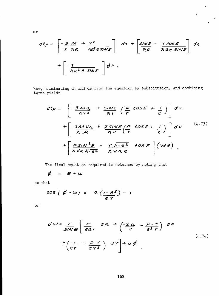
J
or
IN E - "I"C05E "7 de
_ --_N_'J
÷[-'r ]at'.1lo.. Z e ..51ALE
Now, eliminating d_ and de from the equation by substitution, and combiningterms yields
]_ V o... e
(a.73)
The final equation required is
so that
eos ( # - _)
or
: a.(,,-e2)eY"
obtained by noting that
- F"
Fd&V= _ / P 0'0-
_,_(___o,-..*-")
d_
(a.%)
158
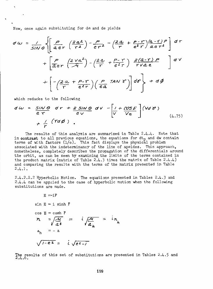
Now, once again substituting for da and de yields
+
which reduc%s to the following
d_cJ = .SIAIOew" o'w" "-/--2.SI/VS_V dV -[__4-C05EI_Vd_)V_ "
/ (rd._)
),-
(_.75)
The results of this analysis are summarized in Table 2.4.4. Note that
in contrast to all previous equations, the equations for dtp and dw containterms of with factors (l/e). This fact displays the physic&l problem
associated with the indeterminancy of the line of apsides. This approach,
nonetheless, completely describes the propagation of the differentials around
the orbit, as can be seen by examining the limits of the terms contained in
the product matrix (matrix of Table 2.&.3 times the matrix of Table 2.A.&)
and comparing the results with the terms of the matrix presented in Table
2.4.1.
2.4.2.2.2 Hyperbolic Motion. The equations presented in Tables 2.4.3 and
2.&.& can be applied to the case of hyperbolic motion when the following
substitutions are made.
E =-iF
sin E = i sinh F
cos E = cosh F
= LX4 --
a h = - a
k/l-ez = _ ,J__l
The results of this set of substitutions are presented in Tables 2.&.5 and2._.6.
159
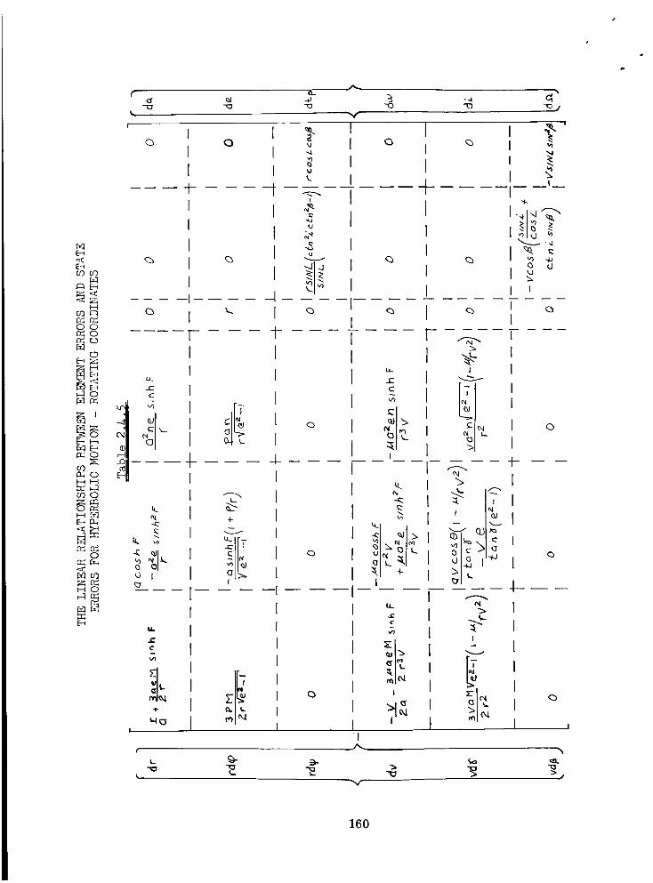
t- Q-
o 0
L
t
i l i %
I I I '
I
E_
cOcO
_E_
O0_0___
0_-_
)-4O
I--41--4
0
NO
_5
c-
C
II
I
I-1
I I
_k u... __ _clrl
0, I I
----[ .... II I
" I I
,. I I
!
r
t. _-
II
I
I¸ _
II II "
, 1
IT _
!
-t--
" 2 ?I ,_ i% '
I " _1_1 _1_1_ I_I" I _ _ _'_ I
_:ill _I_'_
0
(:3
<:}
lJ
J
160
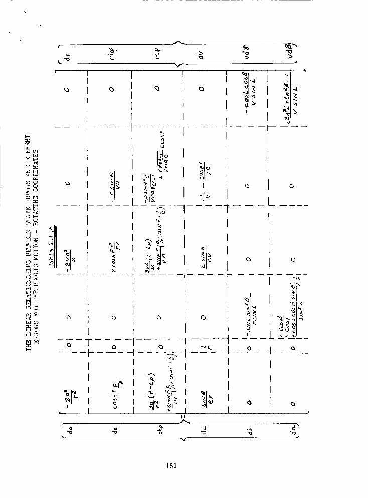
i-
g.
E_
f-_l E--,
o30 (__:_0Or._)I:_
I---t
E--_O
II_"
_0
HFx_
C_C_O
r_r_
O
E-_
_1_!
I-
II
I1II
II
I
IT
"t:3
U.
0
0
_.1_,i
(-vI
o
I I
II 1I I
I- _- FI.j
, _1o ,itl ,_.
I ,.,_
I _1_iI. _
"-" 1I _-
1.1..
I
11I
_1_7-
I
I
_l_ II
I I
l II II
I 1-
t _-t-I *
.- I
I _ _ I _i_'__k
I _1_ _ II _" "_ I III
3
il•'.4 ".
I
° I
:1'_1",
__ °____1
-..t
_1. _
_j
0
0
"1<
?
0
161
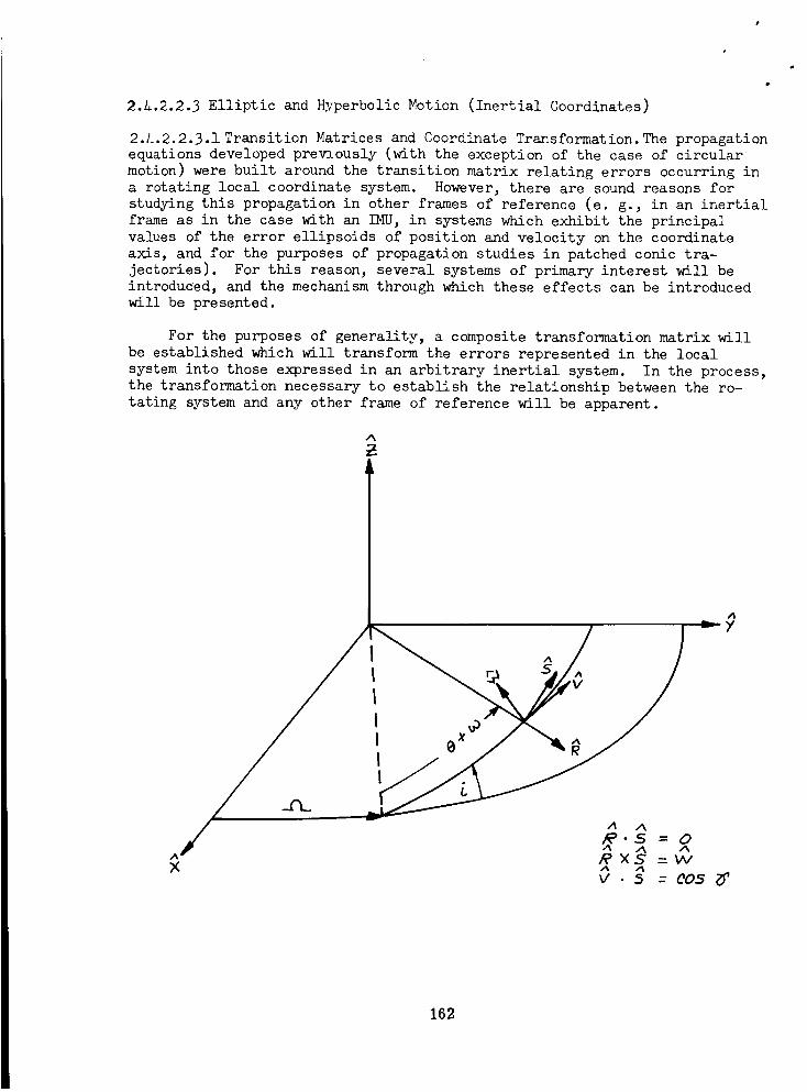
2.4.2.2.3 Elliptic and Hyperbolic Motion (Inertial Coordinates)
2.1;.2.2.3.1 Transition Matrices and Coordinate Transformation. The propagation
equations developed prevlously (with the exception of the case of circular
motion) were built around the transition matrix relating errors occurring in
a rotating local coordinate system. However, there are sound reasons for
studying this propagation in other frames of reference (e. g., in an inertial
frame as in the case with an IMU, in systems which exhibit the principal
values of the error ellipsoids of position and velocity on the coordinate
axis, and for the purposes of propagation studies in patched conic tra-
jectories). For this reason, several systems of primary interest will be
introduced, and the mechanism through which these effects can be introducedwill be presented.
For the purposes of generality, a composite transformation matrix will
be established which will transform the errors represented in the local
system into those expressed in an arbitrary inertial system. In the process,
the transformation necessary to establish the relationship between the ro-
tating system and any other frame of reference will be apparent.
A
162
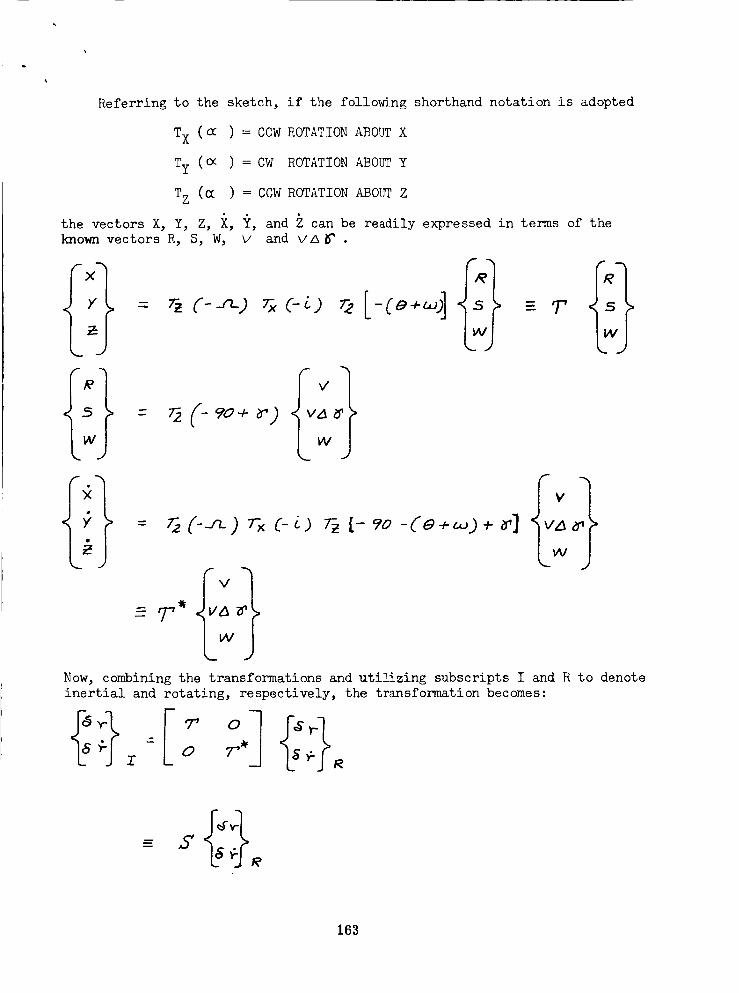
Referring to the sketch, if the following shorthand notation is adopted
Tx (_ ) = COW ROTATION ABOUT X
Ty (_ ) = CW ROTATION ABOUT Y
TZ (_ ) = CCW ROTATION ABOUT Z
the vectors X, Y, Z, i, Y, and Z can be readily expressed in terms of the
known vectors R, S, W, v and VA_ .
rz (-_n..j C-LJ
Now, combining the transformations and utilizing subscripts I and R to denote
inertial and rotating, respectively, the transformation becomes:
Z O T _ _" R
163
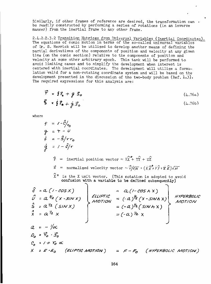
Similarly, if other frames of reference are desired, the transformation canbe readily constructed by performing a series of rotations (in an inversemanner) from the inertial frame to any other frame.
4
2.A.2.2.3.2 Transition _latrj'zc_eA fro_mUni_e£sa! Variables (Inertial Coordinates__.The equations of conic motion in terms of the so---l_al_$-d-_ni_ers_va-ri_s
of Dr. S. Herrick will be utilized to develop another means of defining the
partial derivatives of the components of position and velocity at any given
time (on the conic section) relative to the components of position and
velocity at some other arbitrary epoch. This task will be performed to
avoid limiting cases and to simplify the development when interest is
centered with inertial coordinates. The development will utilize a formu-
lation valid for a non-rotating coordinate system and will be based on the
development presented in the discussion of the two-body problem (Ref. 1.3).
The required expressions for this analysis are:
wh ere
A
_- -- R-- U
-F = --_/Y'ro
: = /- C_/r
r : inertial position vector = XX + + Z
A
X _
= noz_alizedvelocityvector--_/_/_--(X_
is the X unit vector. (This notation is adopted to avoid
confusion with a variable to be defined subsequently)
_' =o..C/ -eos x)A
u - o_._/._(_'-5/NX).4
s = _ '/2.(S/NX).4X =agZX
0__ = - //oC
Do : _-o "-So
eo =/+root
X : E'Eo
EL LIPTI
AgO T/ON
= o..(/-eos/,x_
C-_z.)_C_-__,_x)[
C-_?_ (s/A//_ x)
C-co) '/2.x
H YPERBOL IC
1140 T/ON
(EZ/Pr/C /V/0rl0N ) = :"- ,co {#Y,°£RBOZ/C /I_0TION..)
164
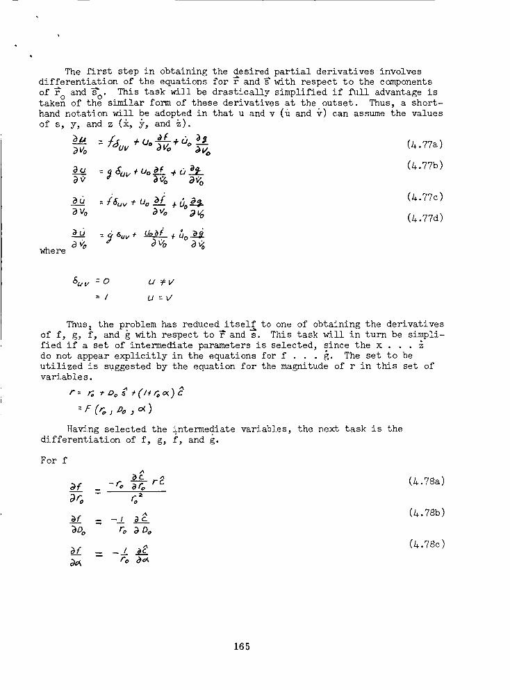
The first step in obtaining the desired partial derivatives involvesdifferentiation of the equations for _ and T with respect to the componentsof_ ° and_ o. This task will be drastically simplified if full advantageistaken of the similar form of these derivatives at the outset. Thus, a short-hand notation will be adopted in that u and v (Q and v) can assumethe valuesof s, y, and z (_, y, and _).
where
(/+.77a)
Bu =_5ov÷Uo a¢ 4u_:- (A.77b)
_vo Bvo 9_ (&.77d)
÷
_uv :O U _V
=1 U:V'
Thus_ the problem has reduced itself to one of obtaining the derivativesof f, g, f, and g with respect to T and s. This task will in turn be simpli-
fied if a set of intermediate parameters is selected, since the x . .
do not appear explicitly in the equations for f . g. The set to be
utilized is suggested by the equation for the magnitude of r in this set ofvariables.
=F(_jDoj_)
Having selected the intermediate variables, the next task is the
differentiation of f, g, f, and g.
For f
A
-to _ rc (z_.78a)
,4.
_Do ro _ _o
(A.78b)
(z_.78c)
165
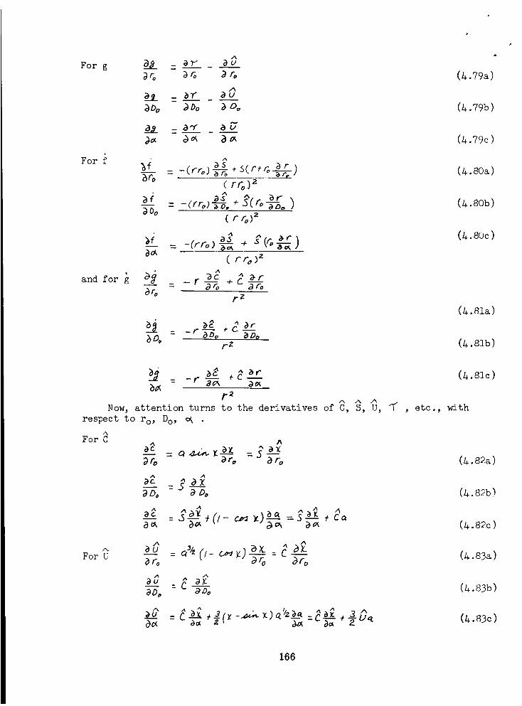
For g
For
i
and for g
a_& ar aul -- -- --
aG a_ a&
A
_Do _ Do _ Oo
_ro -gT; * )(fro) 2
) Do( r to) 2
/-- = _ _ .ad,
(rQ) z
a_ -r Tg +aro
r z
Do _-_ a--_FZ
(/4..79a)
(_.79b)
(_.79c)
(4.80a)
(4.80b)
(4.8oc)
(4.sla)
(4.83_b)
raA .A/%
Now, attention turns to the derivatives of C, S, U,
respect to ro, Do,
A
For C
_-5o= a_o
A A
_- 3 _ )_:s _--_,c_a--a = ga ' (/- e''a z a_
Fora_
a,'oa$= a,/,(./_ _)-a-go a--_
a_a :e a_'ao_ az)_
- - U,a.
/'_ },
(4.81c)
etc., with
(g.82a)
(g.82c)
(4.83a)
(4.83b)
(4.83c)
166
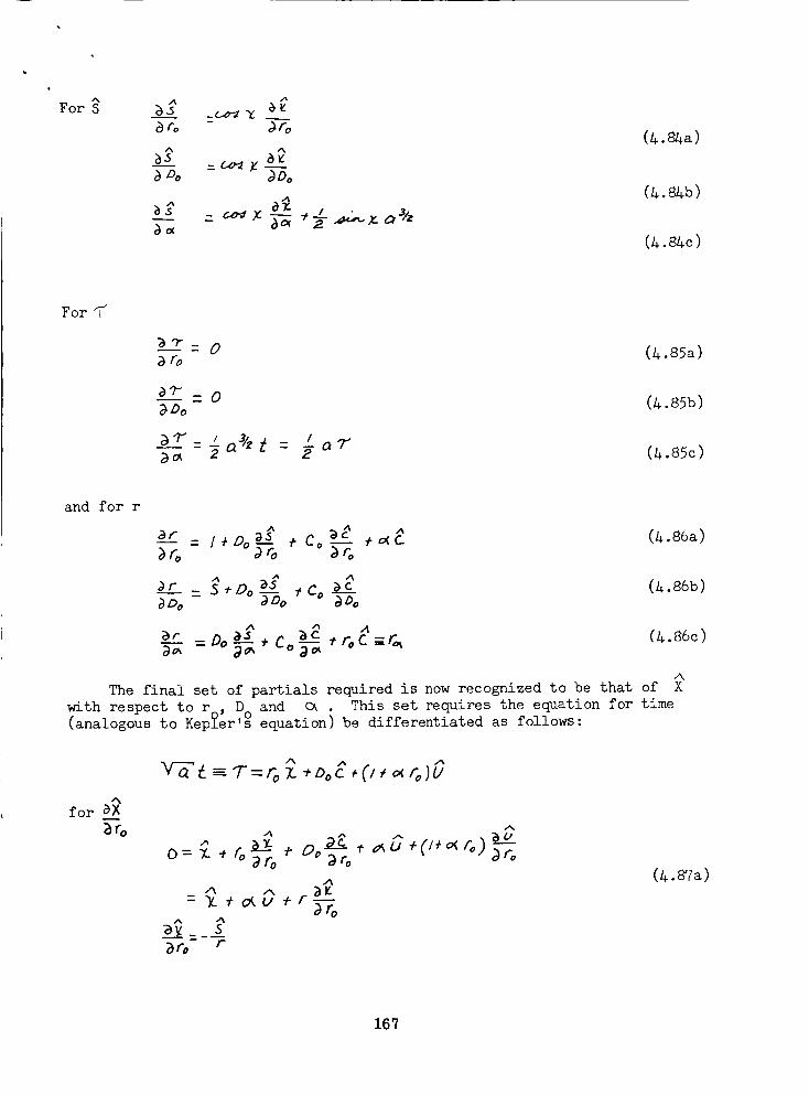
For
8Zo - _fo
B5 c_y aza--So - _--_o
(a._a)
(L_.84b)
(_.8_c )
For fi_
--- 0_Do (4.85b)
and for r
-- = /+Do + Co ¢_C (/_.86a)
a__c_r= __,Do _f ^
A _ A
ar --Do _s _a (4.86c)
A
The final set of partials required is now recognized to be that of X
with respect to r , D and c_ . This set requires the equation for time
(analogous to Kep_er'_ equation) be differentiated as follows:
A _ A
for B_X
_ro A
" _- , -- _ _u +(/+_ro) _0=_ +roar ° ° _ro _o
A
= _ + _ v + r _--7_
_r_ r
(A.&/a)
16_
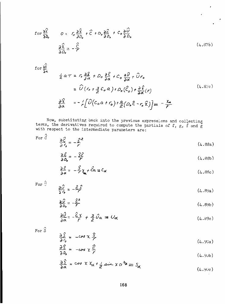
A
for _--_-_o
a_E c_)D.- F
(_.STb)
p
A
for __X
alt = - U Coo__ r
(_.87c)
Now, substituting back into the previous expressions and coll.ectin_terms, the derivatives required to compute the partials of f, g, f and g
with respect to the intermediate parameters are:
A
For C A_C __z- - 0+. 88a )_rD r
A
For U
A ^Z
__._u= _C_G_ (&. 89b)9 Do r
A
_)u_ c_ + _0__ t)_ (_-._9o)
For S
3% r
_Do r
a_
(4.90a)
(A.9Ob)
(_._uc)
168
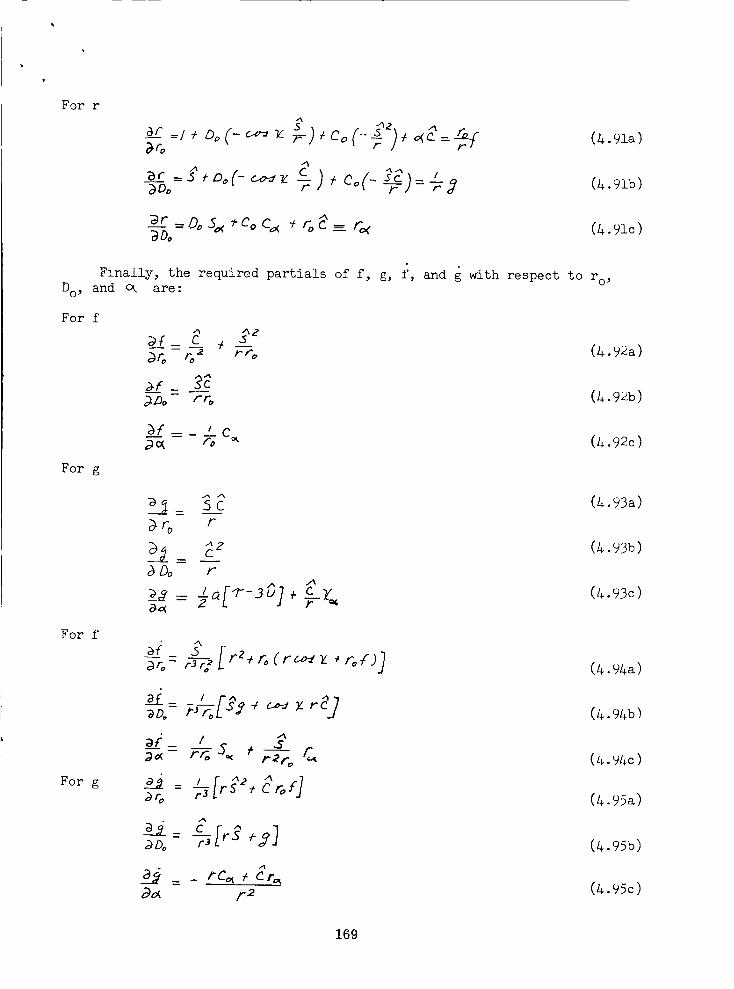
For r
Do_
For f
For g
For f
For g
aro
_Oo 7 73
(_.gla)
(4.91b)
(4.91c)
Finally, the required partials of f, g, f, and g with respect to ro,and _ are:
A _Z
_f_c_ ÷!_ ro ro _ fro
bf-_±c
(4.92a)
(L.. 9_b)
(4.92c)
_= c_z_Do r
, [_-30 8a,_
(4.93a)
(4.93b)
(4.93c)
2to- r3r# ÷ _ (r_ z ÷ rof)
ai / __
_r_ ra
_Oo rS
3_ f_
(4._4a)
(4.94b)
(4.95b)
(4._5c)
169
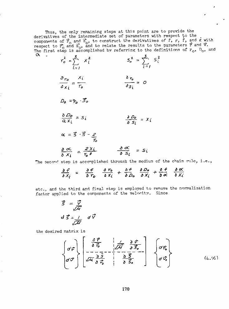
Thus, the only remaining steps at this point are to provide thederivatives of the intermediate set of parameters with respect to the
components of __ and To, to construct the derivatives of f, F, f, and _ with
respect to r'o a_d _o, and to relate the results to the parameters r and 9".The first step is accomplished by referrin_ to the definitions of ro, Do, and
z 3 3 Z
_=1 l=l
Dro X_ 6 ro"_ _ 0
axL ro DsL
Do =_'o .50
Do - 5 _ a Do=Xi
o_ =5 "5-2
ro
a oc 2X__L a oC =5,'o x_ - ro 3 a 5 L
The second step is accomplished through the medium of the chain t_]_e, i.e.,
etc., and the third and final step is employed to remove the normalization
factor applied to the comoonents of the velocity. Since
._m ..b
S = V
d£=l_d_
the desired matrix is
dV
y-I
I / a_
a-% ]b5llb
50(&.96)
170
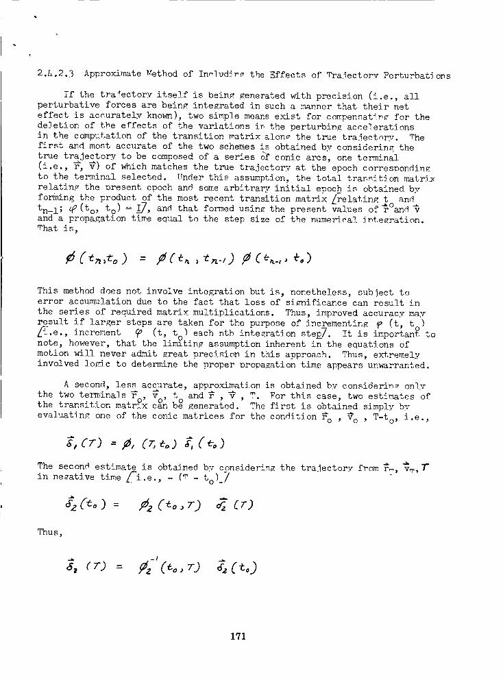
2.1,..2.3 Approximate _.ethod of IncludJn_ the Effects of Trajectory PerturbatJ ons
If the trajectorv itself is being. Fenerated with precision (i.e., allperturbative forces are bein_ integrated in such a manner that their net
effect is accurately known), two simple means exist for compensating, for the
deletion of the effects of the variations in the perturbin_ accelerations
in the computation of the transition matrix alon_ the true trajectc.ry. The
first and most accurate of the two schemes is obtained by considerin_ the
true trajectory to be composed of a series o_fconic arcs, one terminal
(i.e., r-_, _) of which matches the true trajectory at the epoch corresDondin_
to the terminal selected. Under this assumption, the total t.ra_._ition matrix
relatin_ the _resent epoch and some arbitrar_ initial epoch is obtained b.v
forming the product of the most recent transition matrix Zrelatin_ t and-_o
tn_l; @_ (to, to ) = I_, and that formed usin_ the present values of r and -_
and a propagation time equal to the step size of the numerical J_te_ration.
_hat is,
--- ,a' +°)
This method does not involve integration but is, nonetheless, subject toerror acm_nulation due to the fact that loss of significance can result in
the series of required matrix multiplications. Thus, improved accuracy may
result if larger steps are taken for the purpose of incrementin_ _ (t, t^)
_.e., increment _ (t, t ] each nth integration ste_7. It is important, to
note, however, that the lim_tinF assumption inherent in the equations of
motion will never admit _reat precision in this approach. Thus, extremely
involved lo_ic to determine the proper _ropa_ation time appears unwarranted.
A second, less accurate, approximation is obtained by consideri_ only
the two terminals _ , t and _ , _ , T. For this case, two estimates ofthe transition matr°x cV°n b ° _enerated. The first is obtained simply by
evaluating one of the conic matrices for the condition _o , V_o , T-to, i.e.,
The second estimate is obtained by considerin_ the trajectory from _T, Sm, tin necative time _-i.e., - (m _ to) -/
(to) - 7-.2 q cz)
Thus,
1_1
These t_o estimates can now be combined by weighing them in some fashion.
For the case of equal _ights
This second procedure is easily mechanized if the transition matrices
relate inertial errors, since the analytic inverse theorem can be applied to
avoid numerical problems in the process. In fact, this theorem can be
utilized even in those cases where rotating coordinates are employed when it
is noted that the rotating and inertialmatrices are related as follows:
where S (t) is an orthogonal transformation. Thus,
!
The accuracy of the second technique is somewhat unkno_m. From physical
reasoning of the case in which T-t is less than one period, it can be arguedthat the inclusion of the second estimate will provide an improvement in the
accuracy. However, a measure of the improvement is difficult to construct
since the magnitude of the perturbative displacement (secular plus periodic;
resulting from the non-central forces of the problem) from the conic trajec-
tory varies from point to point along the trajectory. For the case where T-t o
is greater than one period, the same effects exist. In addition, errors are
introduced due to the fact that pure conic reference is being assumed for
increasingly long intervals of time.
Another family of approximations can, of course, be generated by com-
bining the first two types.
172
)
2.5 DATA WEIGHTING
2._.] Gen_l _n_o_v
Th_ _m_l_m_nt_tion o_ th_ vsr_ous estimators +ha+ s_e _troduced _n th_s
monograph reouires a knowledge of the cova_an_e matrix of the observables.
Th_s covar_ance matrix can be determined from the covar_anee matrices of in-
strument error_ _nd navigation model errors. Th_s section will present
the general expression that relates thes_ covsr_n_e m_t_ces. The fo]low_n_
seetinn (2.5.2) will Kive th_ det_1_d exo_ess_ons for eseh tv_ of n,_einn
measurement that will exnl4 c_t]y define this cova_iance relat _onship for
any comb_ nati on of nsv_ _mtion measurement.
When a navigation observation is made, it will d_ffer from a predeter-
mined nominal measurement because of several reasons. F_rst, th_ veh_ ele
will be off the nominal trajecto_ by some amount _n both pos_t_on and
velocity. Second. the constants of the navigation model that were used to
calculate the non_inal _.easure_ent a_e themselves _n error, becau,_e of uncer-
ts_nties in th_ physical dimensions and uncertainties _n celestas] body
positions. Finally, the uncerta_hty of the instrument that _s ua_d for themeasurement will constr_bute to the difference _n the messurement.
S_nce all of the sources of the deviations are small and the nominal
measurement _s assumed to be known, the measurement may be exDanded dn a
Taylor Series about the nominal, vaSue by including derivatSves with resD_ct
to all of the variables that _nfluence the measurement.. Furthermore, s_nce
the contrSbution of each deviation source is very small, the higher order
terms may be neglected _n the Taylor Series. Letting _i be the measurement
of interest, the Taylor Series can now be expressed as
where q_o is the nominal value of the measurement
dX is the true state vector deviation
d/_ is a vector comnosed of the model uncertainties
d_ i is the instrument measurement error associated with qiX is the state vector
._s the vector comDosed of the navigation model parameters
__i ds the vector of measurement parameters
Ecuat_on (5.1) can be recognized as a more general form of the pos_t_on
devlat_on e_u, tion thot was presented in a previous monograph. Reference 1.1.
It _s recalled that a deviation in some observation from s nominal value
could be related to the _osition deviation as follows:
173
b
where 8_ is an observation vector composed of the 6q_'s
qi = ai - qioR = position deviation from nominal
A eomos_son of Eauations (5.1) and (5.2) reveals that Equation (5.2)
corresponds to the second term of Equation (5.1), where the state vector
deviation is considered to be oos_t_on deviation only. The significance ef
all of terms _n Eauation (5.1) should now be ao_arent. The first term _s
merely a predetermined auantlty that gives the value of the auantlty under
perfect condSt_ons, i.e., that value that would be measured _f the vehicle
were exactly on the nominal trajectory, all positions and dimensions of
objects used for the observation were known exactly, and the instrument
used for the measurement were error free. The second term corresponds to
the deviatlons in the measurement that are due to perturbations of the
state vector about the mom_nal trajectory. The thCrd term represents all
measurement deviations that are _ntroduced bs uncertalnt_es in the navigationmodel. The number of elements _n th_s vector depends on the number of uncer-
tainties in the model that have a direct first order effect on th_ measurement.
Finally, the l_st tp_m _n Eauation (5.1) reores_nts the error due to the
u_certa_nti_s _n the _nstrument that is used for the it_h measurement. In
cases where the navigation observable and the measured quantity are the same,
the vector _ will merely contain a "one" in the appropriate location.
However. _f the messu_ed auantity and the navigation observable differ, as
_n radar measurements where phase and frenuency measurements are indSrect
and range-rate measurements, then the vector _ must contain therange
appropriate oartial derlvative to account for the uncertainty in the sensor.
If a series of navigation measurements is made. Eauat_on (5.1) can be
extended to a vector eouation.
b_ -- _ ÷ dE
It sho_1 d be noted that the model uncertainty term _s now shown as the pro-
duct of a matrix, _ and a vector dM. This notation can be adopted becaus
molel uncertainties, even though they all may not be used for a particular
observation, may be entered into a column vector. If a particular model
uncsrtainty _s not used for an observation, then the _ matrix will con-
tain zeroes in the appropriate locations. _-_
The covariance matrix for _ can be found by employing the expectedvalue theorem. (See Appendix A.) The result is
174
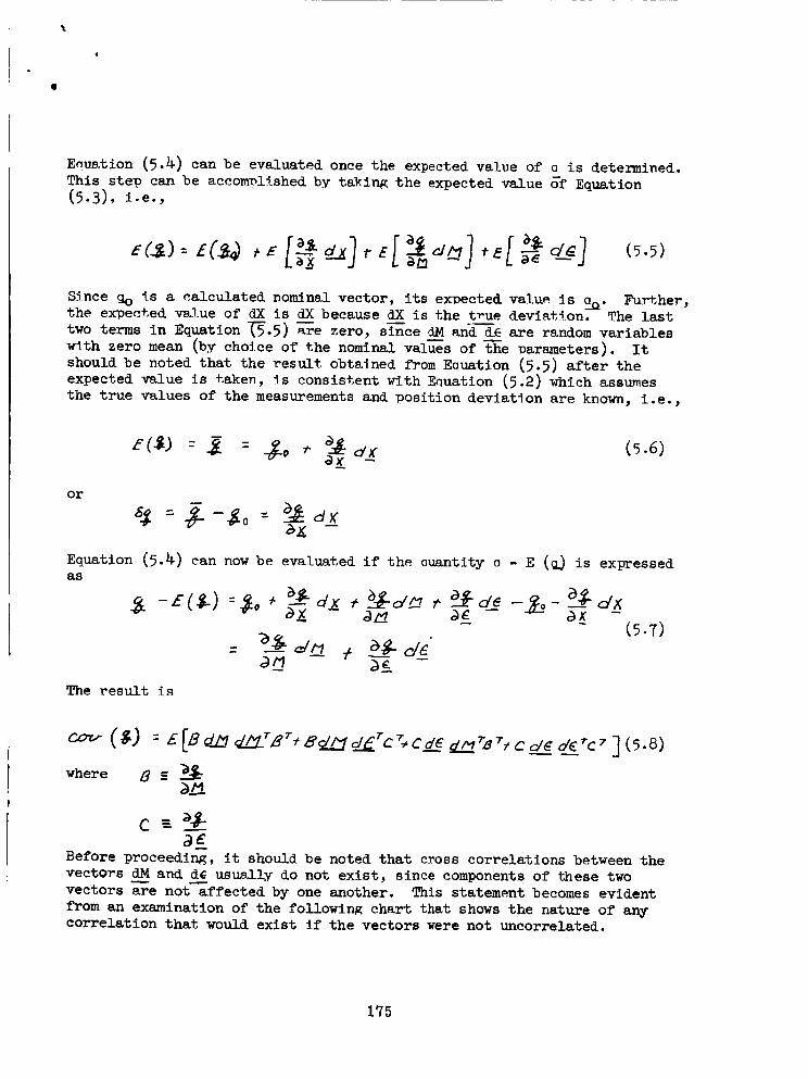
@
Eauation (5.4) can be evaluated once the expected value of a is determined.
This step can be accomplished by taking the expected value of Equation(5.3), i.e.,
(5.5)
S_nce go _s a calculated nominal vector, its exoected value is ao. Further,the exoeeted value of dX is dXbecause dX is the true deviat_ou. The last
two terms in Equation_.5) a-re zero, si-nce dM and-_E are random variables
_th zero mean (by choice of the nominal vales of t--heDarameters). It
should be noted that the result obtMned from Eauation (5.5) after the
expected value is taken, _s consistent with Eauation (5.2) which assumes
the true values of the measurements and _osition deviation are known, i.e.,
_K -(5.6)
or
Equation (5.4) can now be evaluated if the auantity o - E (_ is expressedas
a_ dX ," a._o,'_ ,'- o__de -.._- as. dx
: __-_ ÷ a_a_/__'(5.T)
The result is
Before proceeding, it should be noted that cross correlations between the
vectors dM and d__ usual3_v do not exist, since components of these two
vectors are not affected by one another. This statement becomes evident
from an examination of the followin_ chart that shows the nature of anycorrelation that would exist if the vectors were not uncorrelated.
1'75
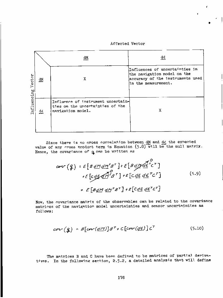
O
Affected Vector
o4o
O
.r
dM
d_
dM d£
X
Influence of _nstrument uncertain-
t_es on the uncertainties of the
uavIKation model.
[nfluences of uncertainties in
the navigation model on the
accuracy of the instruments _sedin the measurement.
X
Since there _s no cross eorrelatlon between dM and d£ the ex_eeted
value of any _oss nroduct term in E_uatdon (5.8)--_11 b_-the null matrix.
Hence, the covar_auce of _ cad be written as
O
o(5.9)
Now, the eovar_ance matrix of the observables can be related to the covar!ance
matrices of the navigation model uncertainties and sensor uncertainties as
follows:
The ms,trices B and C have been defined to be matrices of partial derlva-
t_ves. In the followin_ section, 2.5.2, a detailed ana].ysis thRt will define
176
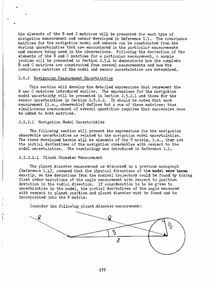
the elements of the B and C matrices will be presented for each type of
navigation measurement and sensor developed in Reference 1.1. The covariance
matrices for the navigation model and sensors can be constructed from the
various uncertainties that are encountered in the particular measurements
and sensors being used in the observations. Following the derivation of the
elements of the B and C matrices for a particular measurement, a sample
problem will be presented in Section 2.5._ to demonstrate how the completeB and C matrices are constructed from several measurements and how the
covariance matrices of the model and sensor uncertainties are determined.
2.5.2 Navigation Measurement Uncertainties
This section will develop the detailed expressions that represent the
B anc C matrices introduced earlier. The expressions for the navigation
model uncertainty will be presented in Section 2.5.2.1 and those for the
sensor uncertainties in Section 2.5.2.2. It should be noted that each
measurement (i.e., observable) defines but a row of these matrices; thus
simultaneous measurement of several quantities requires that successive rowsbe added to both matrices.
2.5.2.1 Navigation Model Uncertainties
The following section will present the expressions for the navigation
observable uncertainties as related to the navigation model uncertainties.
The terms developed herein will be elements of the B matrix, i.e., they are
the partial derivatives of the navigation observables with respect to the
model uncertainties. The terminology was introduced in Reference 1.1.
2.5.2.1.1 Planet Diameter Measurement
The planet diameter measurement as discussed in a previous monograph
(Reference 1.1), assumed that the physical dimensions of the model were known
exactly, so the deviations from the nominal trajectory could be found by taking
first order variations of the angle measurement with respect to position
deviation in the radial direction. If consideration is to be given to
uncertainties in the model, the p_rtial derivatives of the angle measured
with respect to planet position and planet diameter must be found and be
incorporated into the B matrix.
Consider the following planet .diameter measurement:
lq7
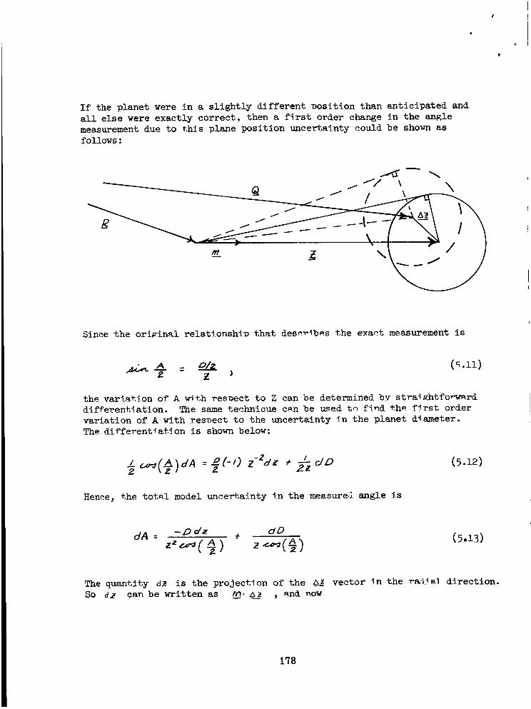
0
B
If the planet were in a slightly different Dosltion than anticipated and
all else were exactly correct, then a f_rst order change in the anglemeasurement due to this plane position uncertainty could be shown as
follows:
Since the original relationshio that desn_bes the exact measurement is
_ D/a (_.ll)Az- Z
the variation of A w__th resDect to Z can be determined by straightforward
differentiation. The same teehniaue can be used to f_nd the first order
variation of A with resneet to the uncertainty in the planet diameter.
The differentiation is shown below:
, --
Hence, *,he total model unee_ainty in the measure& angle is
(5.12)
dA = -D dz dO+ (5.13)
The quantity d,_ is the projection of the b! vector _n the ra,;.:_al direction.
So d,.Z ca_ be written as n'l. A_Z , and now
178
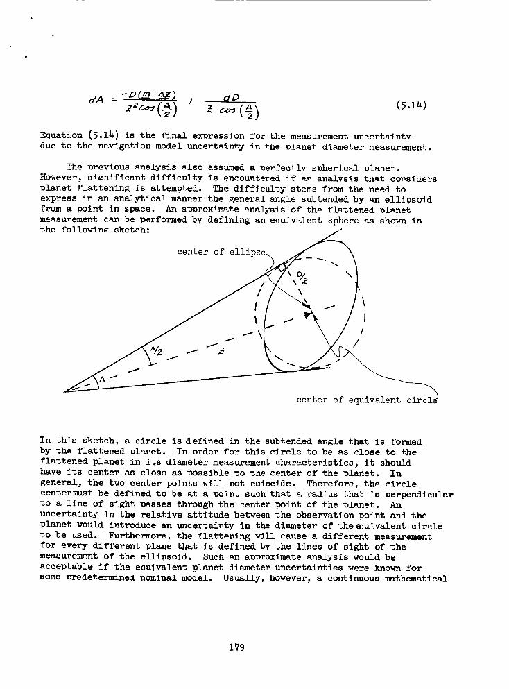
4
E_uation (5.14) is the final expression for the measurement uncertaintv
due to the navigation model uncertainty -in the olanet, diameter measurement.
The _revlous sna_vsis slso assumed a _erfectl_ s_herical olanet.
However, s_n_f_cant difficulty _s encountered if an analys_s that considers
planet flattening is attempted. The difficulty stems from the need to
express in an analytical manner the general angle subtended by an ellipsoid
from a _oint in space. An ao_rox_m_e _nalys_s of the flattened _lanet
measurement can be performed by defining an enuivalent sphere as shown _nthe followin_ sketch:
)
In th_s sketch, a circle is defined in the subtended angle that is formedby the flattened olanet. In order for this circle to be as close to the
flattened planet in its d_ameter measurement characteristics, it should
have its center as close as possible to the center of the planet. In
general, the two center points will not coincide. Therefore, th_ circle
centermust be defined to be at a _o_nt such that a radius that Is _erpend_cular
to a line of s_ght. _sses through the center point of the planet. An
u_certainty _n the relative attitude between the observation _olnt and the
planet would introduce an uncertainty in the diameter of the_u_valent c_rale
to be used. Furthermore, the flattening will cause a different measurement
for every different plane that is defined by the lines of s_ght of the
measurement ofthe elli_sold. Such an a_rox_mate analysis would be
acceptable if the esu_valeut planet diameter uncertainties were known for
some oredetermined nominal model. Usually, however, a continuous mathematical
179
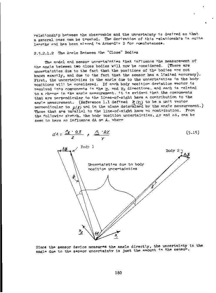
relatlonsh_p between the observable and the uncertainty is desired so that
a general case can be t_eated. The derlvation of thls _elationshi_ _s nu_+,e
le_+hv _nd h_s been o]_e_d _n A_oend_ D _or completeness.
2.5.2.1.2 The A_=le Between the "Close" Bodies
The model and sensor unee_talnt_s that _ngluenee the measurement of
the angle between two close bodies will now be considered. (There are
uncertainties due to the fact that the positions of the bodies _re not
known exactly, and due to the fact that the sensor has a llmited accuracy).
First, the uncertainties in the an_le due to the uneertalnties in the bo_v
nositions w-ill be considered. If e_eh body nosition deviation vector is
resolved _nto components In ehe _, _nd _z d_rect_n_s, and _aeh Is _e]_ted
to & eh_g_ in eh_ an_]e me-surement. _t is ev/dent that the components
that are perpendicular to the lines-of-sight have a contribution to the
an_]_ measurement. (Reference i.i deflned _ (_z) to be a unit vector
Dernendicular to _(Z) and in the nlane determined by the saK]e measurement. )Those that are nara]lel to the line-of-sight have no contribution. From
the fol]owID_ s_eteh, the bo<v oosition uncertainties, AY and _z, can be
seen to have a_ influence dA o_ A, _zhere
_/ Body 1
Body 2
U_certaint_es due to body
nos_ti on uncertainties
Since the sensor device measures the angle directly, the uncertainty in the
angl_ due to the s_n_or uncertaint_ is Just the _ount In the sensor.
180
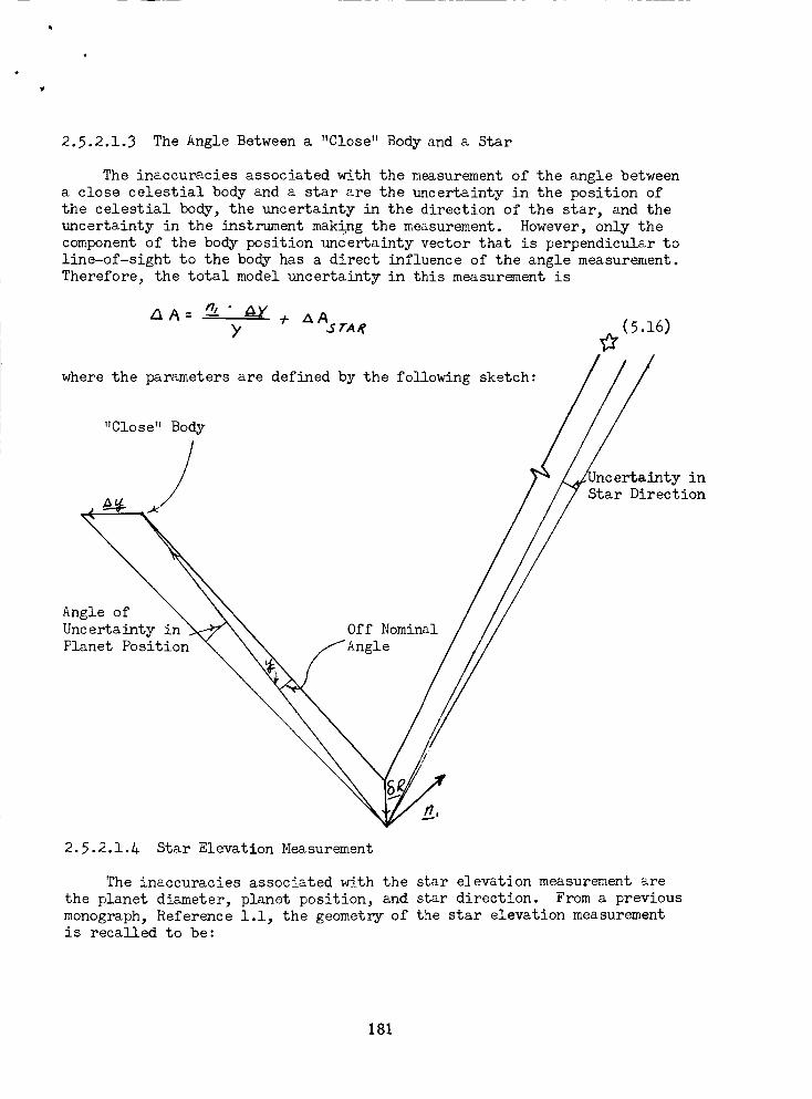
Q
2.5.2.1.3 The Angle Between a "Close" Body and a Star
The inaccuracies associated with the measurement of the angle between
a close celestial body and a star are the uncertainty in the position of
the celestial body, the uncertainty in the direction of the star, and the
uncertainty in the instrument making the measurement. However, only the
component of the body position uncertainty vector that is perpendicular to
line-of-sight to the body has a direct influence of the angle measurement.
Therefore, the total model uncertainty in this measurement is
where the parameters are defined by the following sketch:
inStar Direction
Angle of
Uncertainty inPlanet Position
Off Nominal
2.5.2.1.A Star Elevation Measurement
The inaccuracies associated with the star elevation measurement are
the planet diameter, planet position, and star direction. From a previous
monograph, Reference 1.1, the geometry of the star elevation measurementis recalled to be:
181
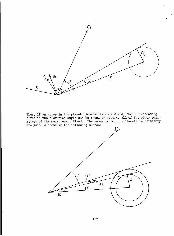
£ A
Thus, if an error in the planet diameter is considered, the corresponding
error in the elevation angle can be found by keeping all of the other para-
meters of the measurement fixed. The geometry for the diameter uncertainty
analysis is shown in the following sketch:
182
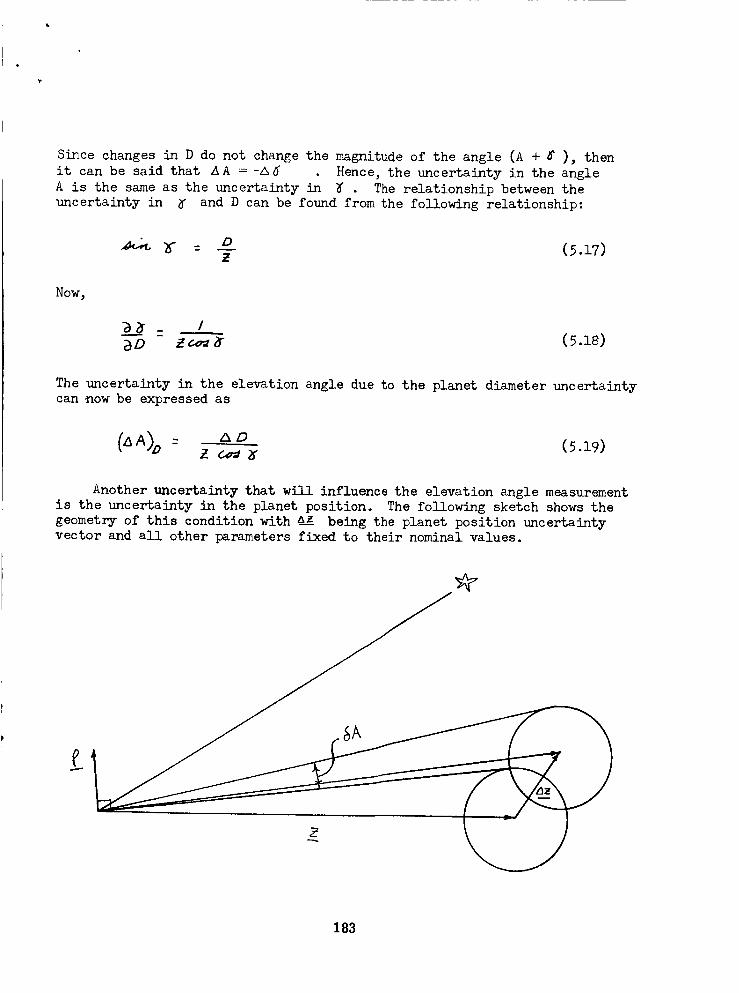
Since changes in D do not change the magnitude of the angle (A + 8 ), then
it can be said that AA =-&6 . Hence, the uncertainty in the angle
A is the same as the uncertainty in _ . The relationship between the
uncertainty in _ and D can be found from the following relationship:
_ D (5.17)
Now,
The uncertainty in the elevation angle due to the planet diameter uncertaintycan now be expressed as
AA) D _- Z_DZ _ ; (5.19)
Another uncertainty that will influence the elevation angle measurement
is the uncertainty in the planet position. The following sketch shows the
geometry of this condition with _ being the planet position uncertaintyvector and all other parameters fixed to their nominal values.
183
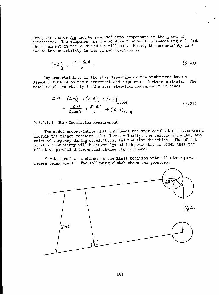
Here, the vector AZ can be resolved into components in the _ anddirections. The co--mponent in the __P direction will influence angle A, but
the component in the Z direction will not. Hence, the uncertainty in A
due to the uncertainty in the planet position is
Any uncertainties in the star direction or the instrument have adirect influence on the measurement and require no further analysis.
total model uncertainty in the star elevation measurement is thus:
The
_ a o ÷ # .a__z(5.21)
2.5.2.1.5 Star Occulation Measurement
The model uncertainties that influence the star occultation measurement
include the planet position, the planet velocity, the vehicle velocity, the
point of tangency during occultation, and the star direction. The effect
of each uncertainty will be investigated independently in order that the
effective partial differential change can be found.
First,
meters being exact.
consider a change in the _anet position with all other para-
The following sketch shows the geometry:
k
184
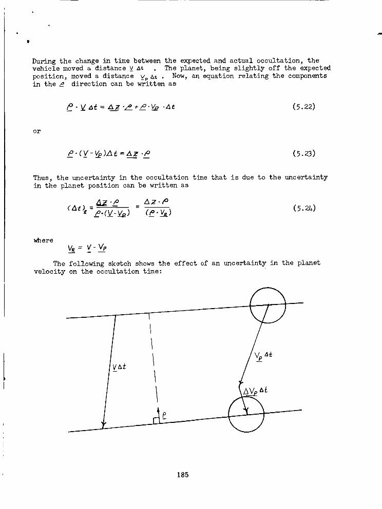
I
During the change in time between the expected and actual occultation, the
vehicle moved a distance y At The planet, being slightly off the expected
position, moved a distance vp A_ • Now, an equation relating the componentsin the _ direction can be written as
(5.22)
or
Thus, the uncertainty in the occultation time that is due to the uncertainty
in the planet position can be written as
where
VR: v- v'p
The following sketch shows the effect of an uncertainty in the planet
velocity on the occultation time:
185
A completely analogous derivation can be performed for this case. Here
AV2A _ is the additional distance that the planet travels during the
time difference between the expected and the actual occultation.
The equation for the components in the _ direction becomes:
(5.25)
In order to determine the differential that___ introduces in a_ , the
occultation time deviation, it is necessary to find the deviation without
_a • This requirement introduces a problem since there would be no time
deviation if all parameters were exactly correct during the occultation.
Yet,the partial differential change is desired, requiring that all parameters
other than those being considered be assumed known. The paradox can becircumvented if a fictitious _t is assumed to exist. 8t is the result
of some parameter being off nominal. This parameter will not be specified
since the parameter being considered, _ , has already been specified.With _V___p=O__, equation (5.25) becomes
(5.26)
where S_ is the fictitious time deviation. The influence of _yp on _Lcan now be determined by subtracting Equation (5.26) from Equation (5.25).
The result is
m.v(4_-s_ }= P. vp(a_-s_) + p.nv m n_ (5.27)
The quantity (AE-8_) can be considered to be the uncertainty in the
occultation time deviation __(AL)v' due to the uncertainty in the planetvelocity.
(A _)vp- e- _re (5.2_)
Where
VR--V-V P
The uncertainty in the vehicle velocity can be handled in a manner
similar to that of the planet velocity. The following sketch shows the
geometry:
186

The equation for the components in thee direction becomes
For no inaccuracy in V, the previous expression becomes
(5.30)
where 8b is again the fictitious time deviation discussed earlier. The
uncertainty in the time deviation due to the vehicle velocity uncertainty
can now be found as before by the difference between Equations (5.30) and
(5.29). Solving for the time difference ( At -g_ ), the result is
If the actual point of tangency differs from the nominal point of
tangency during the occultation time, a correction term for this effect
could be included in the time deviation equation. This is pointed out in
Reference 1.1. Since the point of tangency cannot be determined exactly,
there is an uncertainty in the time deviation due to this tangent point
uncertainty. The component of the time deviation, SL , due to the change
of the point of tangency is shown in Reference 1.1 to be
187
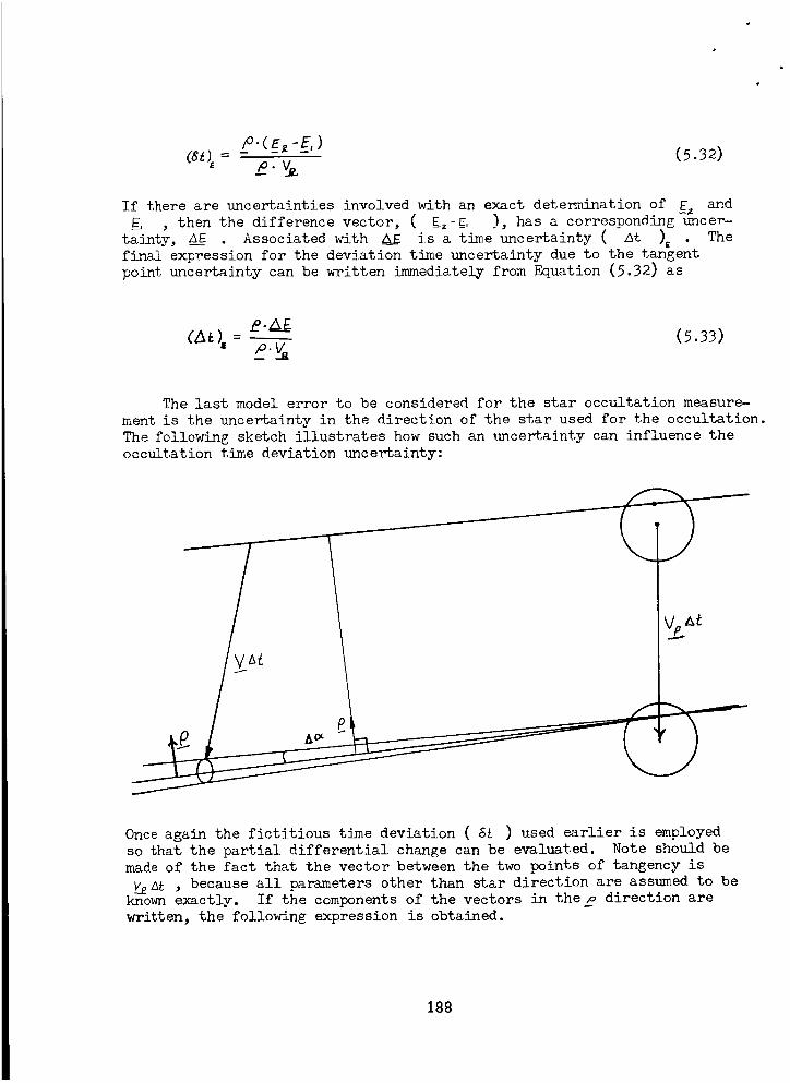
If there are uncertainties involved with an exact determination of _E_ and
_E, , then the difference vector, ( E_-_E, ), has a correspon4ing uncer-
tainty, _ . Associated with AS _Is a time uncertainty ( At )_ The
final expression for the deviation time uncertainty due to the tangentpoint uncertainty can be written immediately from Equation (5.32) as
The last model error to be considered for the star occultation measure-
ment is the uncertainty in the direction of the star used for the occultation.
The following sketch illustrates how such an uncertainty can influence the
occultation time deviation uncertainty:
Once again the fictitious time deviation ( _ ) used earlier is employed
so that the partial differential change can be evaluated. Note should be
made of the fact that the vector between the two points of tangency is
A_ , because all parameters other than star direction are assumed to beknown exactly. If the components of the vectors in the _ direction are
written, the followingexpression is obtained.
188
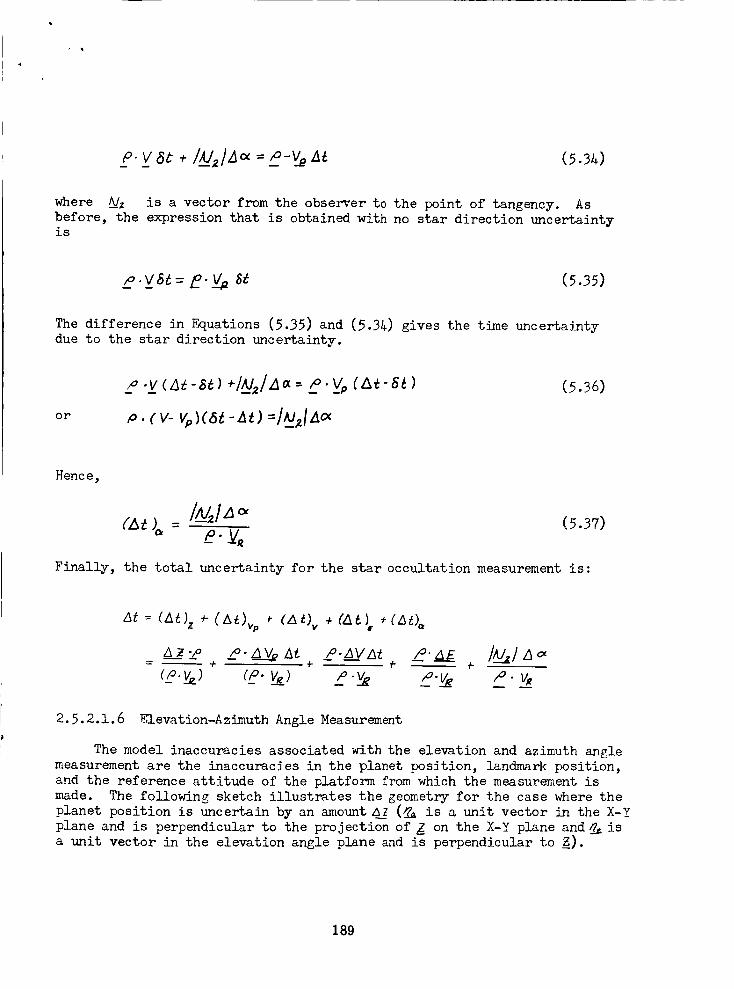
(5.34)
where _ is a vector from the observer to the point of tangency. As
before, the expression that is obtained with no star direction uncertaintyis
The difference in F_uations (5.35) and (5.34) gives the time uncertainty
due to the star direction uncertainty.
or . cv- vp)(a
Hence,
(5.37)
Finally, the total uncertainty for the star occultation measurement is:
2.5.2.1.6 Elevation-Azimuth Angle Measurement
The model inaccuracies associated with the elevation and azimuth angle
measurement are the inaccuracies in the planet position, landmark position,
and the reference attitude of the platform from which the measurement is
made. The following sketch illustrates the geometry for the case where the
planet position is uncertain by an amount A_ (_ is a unit vector in the X-Y
plane and is perpendicular to the projection of Z on the X-Y plane and_is
a unit vector in the elevation angle plane and is perpendicular to _).
189
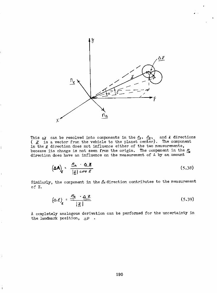
AZ
/
_qcL
This a__zcan be resolved into components in the _a, #g_ and z_directions( _ is a vector from the vehicle to the planet--center). The componentin the _z direction does not influence either of the two measurements,
because its change is not seen from the origin. The component in the ___direction does have an influence on the measurement of A by an amount
Similarly, the component in the_edirection contributes to the measurementof E.
A completely analogous derivation can be performed for the uncertainty inthe landmark position, AP •
190
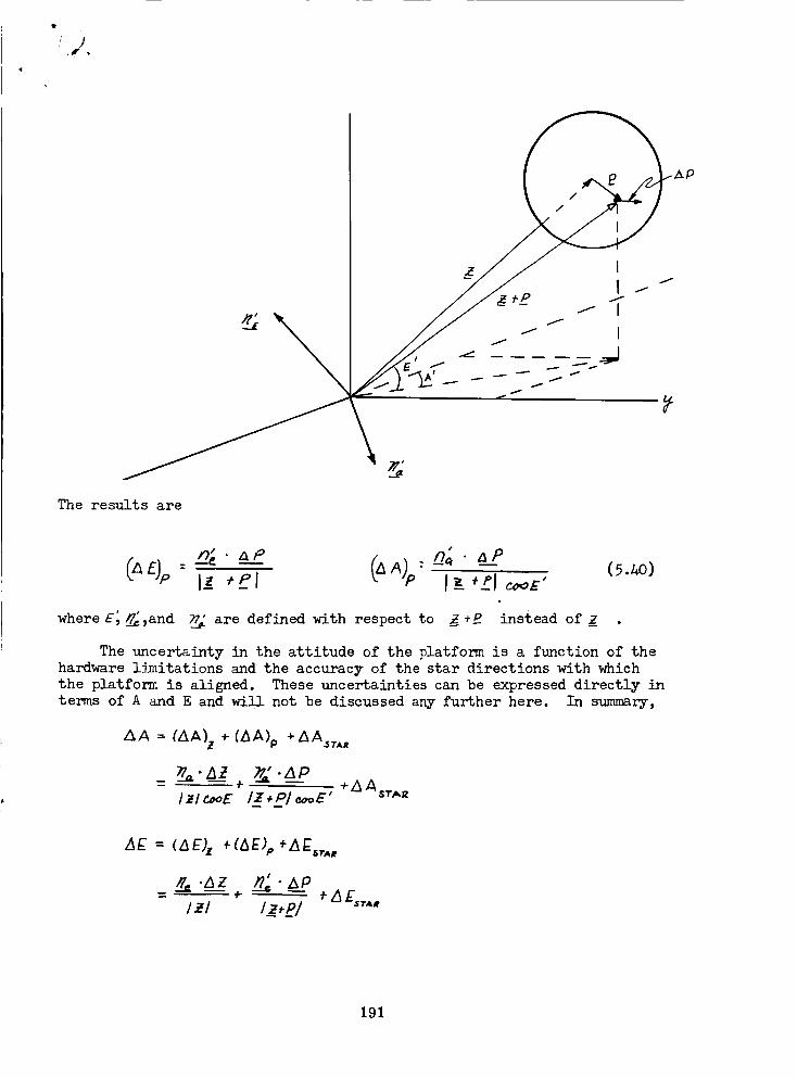
I",i,
The results are
__n_ a___Ps
where E_ _,and _ are defined with respect to _ ÷£ instead of _Z .
The uncertainty in the attitude of the platform is a function of the
hardware limitations and the accuracy of the star directions with which
the platform is aligned. These uncertainties can be expressed directly in
terms of A and E and will not be discussed any further here. In summary,
AA = (AA)z * (AA)p +AAsT.R
I z l c.oeE I t + P l e,o_E "+AAsTAe
z_ = (Z_E)z ,(Z_E),,*aE,,,,,
& .,_z _.&_p-- +.
I ,.,21 I_,B/
191
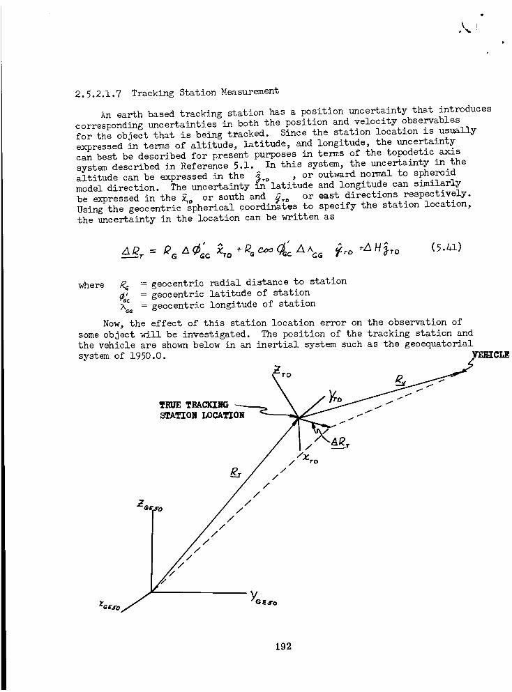
k I
2.5.2.1.7 Tracking Station Measurement
An earth based tracking station has a position uncertainty that introduces
corresponding uncertainties in both the position and velocity observables
for the object that is being tracked. Since the station location is usually
expressed in terms of altitude, latitude, and longitude, the uncertainty
can best be described for present purposes in terms of the topodetic axis
system described in Reference 5.1. In this system, the uncertainty in the
altitude can be expressed in the _To , or outward normal to spheroidmodel direction. The uncertainty In latitude and longitude can similarly
be expressed in the _,° or south and _o or east directions respectively.Using the geocentric spherical coordinhtes to specify the station location,
the uncertainty in the location can be written as
where Rc : geocentric radial distance to station
¢_c = geocentric latitude of station
k_ : geocentric longitude of station
Now, the effect of this station location error on the observation of
some object will be investigated. The position of the tracking station and
the vehicle are shown below in an inertial system such as the geoequatorial
system of 1950.O. ___E_C_
STATION LOCA_ON ___/._
//_ro
////
_, so / //
YGEso
192
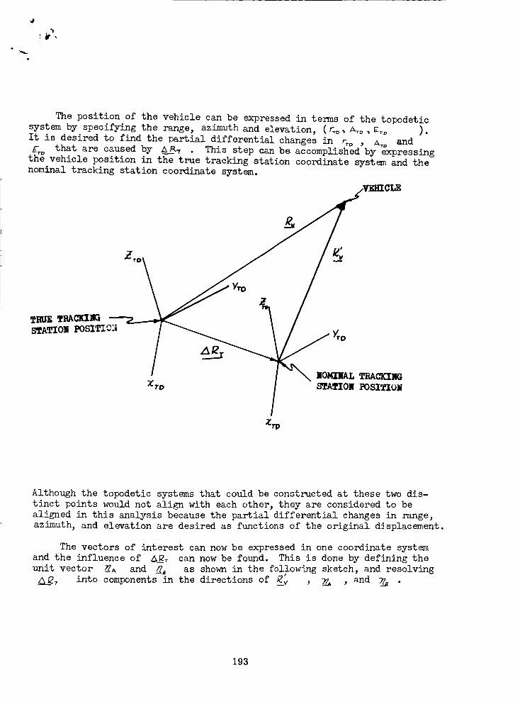
q
The position of the vehicle can be expressed in terms of the topodetic
system by specifying the range, azimuth and elevation, (_o _ ATo _ _ ).
It is desired to find the partial differential changes in r_ , A_ and
t_ that are caused by A R_ . This step can be accomplished by expressingvehicle position in thee true tracking station coordinate system and the
nominal tracking station coordinate system.
Z,o
NOMINAL TRACKING
STATION POSITIOJ
'_rp
Although the topodetic systems that could be constructed at these two dis-
tinct points would not align with each other, they are considered to be
aligned in this analysis because the partial differential changes in range,
azimuth, and elevation are desired as functions of the original displacement.
The vectors of interest can now be expressed in one coordinate system
and the influence of _T can now be found. This is done by defining the
unit vector _A and _ as shown in the following sketch, and resolvingt
____T into components in the directions of _v , __, , and
193
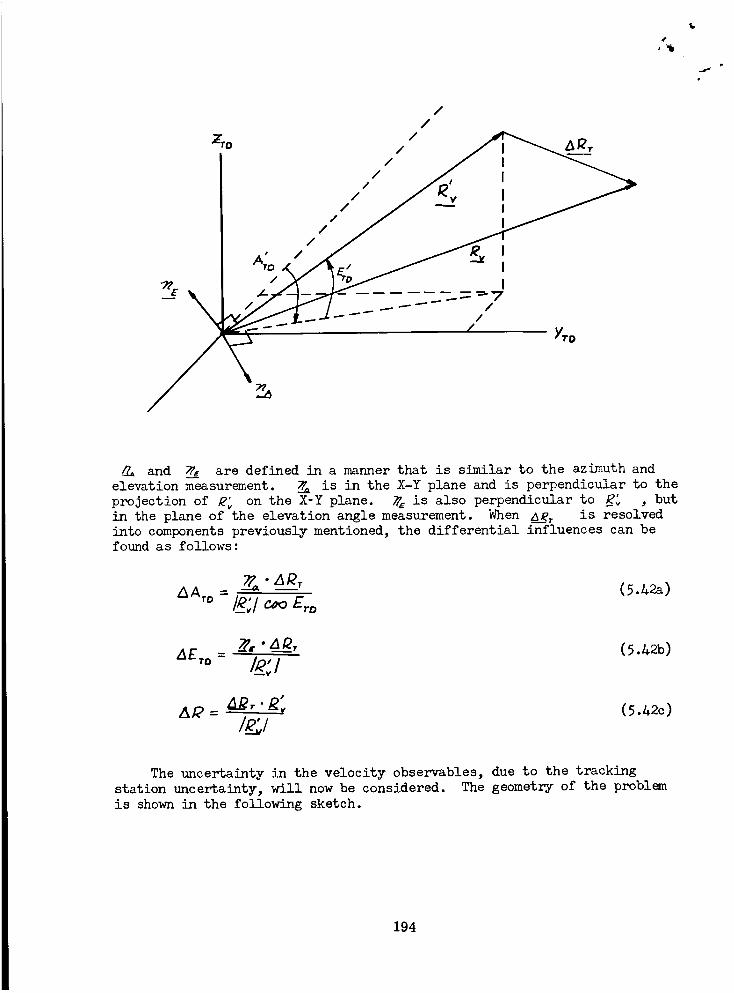
J
_TO
//
( YTo
and _ are defined in a manner that is similar to the azimuth and
elevation measurement. __a is in the X-Y plane and is perpendicular to the
projection of _ on the Xoy plane. _ is also perpendicular to _" , but
in the plane of the elevation angle measurement. _en ___T is resolved
into components previously mentioned, the differential influences can befound as follows :
_ -_R____ (5._)
R." (5. 2b)AE ='°
The uncertainty in the velocity observables, due to the tracking
station uncertainty, will now be considered. The geometry of the proble_
is shown in the following sketch.
194
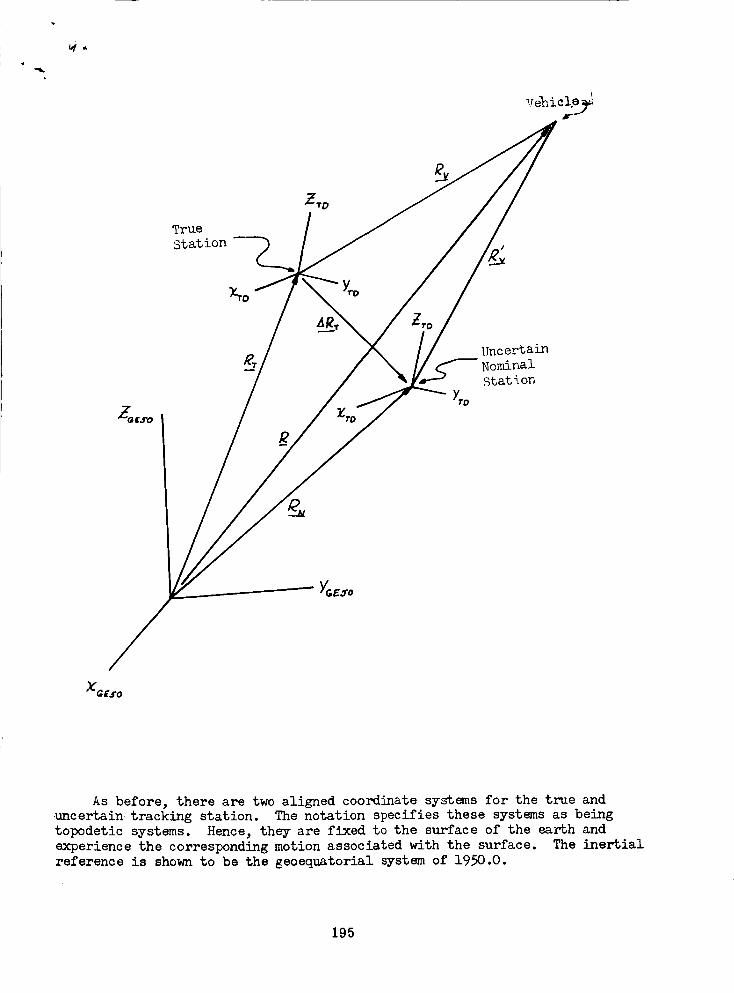
True
Station
Uncertain
Nominal
Stat i on
_G£$0
As before, there are two aligned coordinate systems for the true and
uncertain tracking station. The notation specifies these systems as being
topodetic systems. Hence, they are fixed to the surface of the earth and
experience the corresponding motion associated with the surface. The inertial
reference is shown to be the geoequatorial system of 1950.O.
195
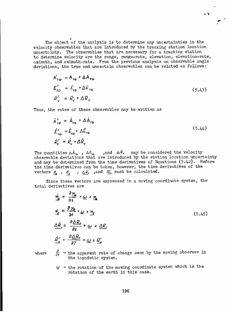
P
The object of the analysis is to determine any uncertainties in the
velocity observables that are introduced by the tracking station location
uncertainty. The observables that are necessary for a tracking station
to determine velocity are the range, range-rate, elevation, elevation-rate,
azimuth, and azimuth-rate. From the previous analysis on observable angle
deviations, the true and uncertain observables can be related as follows:
A'To - ATo * A,A.ro
E;o = Ero *AE,-o
,Q",, = #,,,Aft',,
(5.L,3)
Thus, the rates of these observables may be written as
TO TD TO
4The quantities AA,D , &E,o ,and zx_v may be considered the velocity
observable deviations that are introduced by the station location uncertainty
and may be determined from the time derivatives of F_uations (5.h2). Before
the time derivatives can be taken, however, the time derivatives of the
vectors _ , _ , A_j ,and _ must be calculated.
Since these vectors are expressed in a moving coordinate system, the
total derivatives are
= - "/" G3 X ____.,,-_
_ - the apparent rate of change seen by the moving observer in
the topodetic system.
where
= the rotation of the moving coordinate system which is the
rotation of the earth in this case.
196
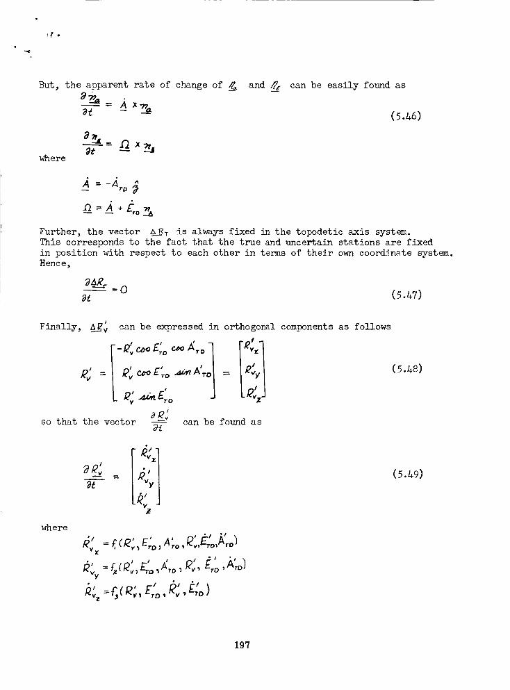
But, the apparent rate of change of __ and can be easily found as
(5.46)
where
=-_o _
Further, the vector __RT is always fixed in the topodetic axis system.
This corresponds to the fact that the true and uncertain stations are fixed
in position _ith respect to each other in terms of their own coordinate system.
Hence,
a_ (5._7)
Finally,I
A_ v can be expressed in orthogonal components as follows
so that the vector _ can be found as
(54.8)
where
LRv ]
Rvz'/= #,,C_.,,,'E;o,A'ro,l_,,,E_.o,A,.o_• j
"' =£_(R,, E' "' "',o,f<,E,o)
(5._9)
197
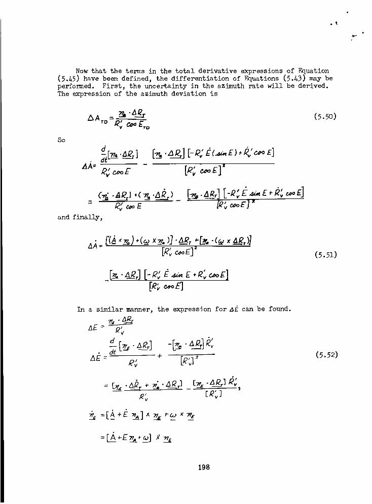
o_
Now that the terms in the total derivative expressions of F_uation
(5._5) have been defined, the differentiation of F_uations (5.&3) may be
performed. First, the uncertainty in the azimuth rate will be derived.
The expression of the azimuth deviation is
_o
JR; E'J
(5._1)
In a similar manner, the expression for 3g can be found.
_E _ ,2v
d
AL:,e,;
: _._. _._ c_.a___._]#;. -- __ •
I
,ev ['q,, ]
(5._2)
198
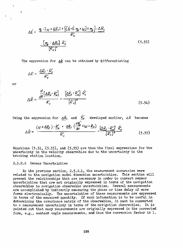
(5.53)
or
The expression for A__ can be obtained by differentiating
Ak)_-__k)___"____',,,%
t Z
(5._#)
• "/
Using the expression for &_ and _-v developed earlier,
-- - e.
&_ becomes
(5.55)
Equations (5.51, (5.53), and (5.55) are thus the final expressions for the
uncertainty in the velocity observables due to the uncertainty in the
tracking station location.
2.5.2.2 Sensor Uncertainties
In the previous section, 2.5.2.1, the measurement accuracies were
related to the navigation model dimension uncertainties. This section will
present the relationships that are necessary in order to convert sensor
uncertainties that are not originally expressed in terms of the navigation
observables to navigation observable uncertainties. Several measurements
are accomplished by indirectly measuring the phase or time delay of wave
forms electronically. The uncertainties of these measurements are expressed
in terms of the measured quantity. If such information is to be useful in
determining the covariance matrix of the observables, it must be converted
to a measurement uncertainty in terms of the navigation observables. It is
pointed out that mar_vmeasurements are originally expressed in the corrected
form, e.g., sextant angle measurements, and thus the conversion factor is 1.
199
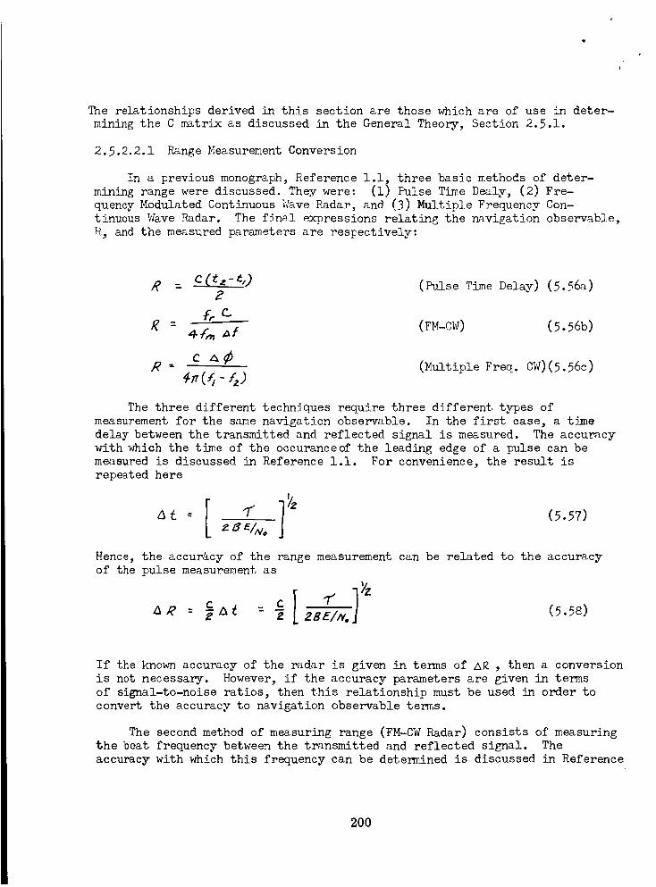
The relationships derived in this section are those which are of use in deter-
mining the C matrix as discussed in the General Theory, Section 2.5.1.
2.5.2.2.1 Range Measurement Conversion
In a previous monograph, Reference 1.1 three basic methods of deter-
mining range were discussed. They were: (ii Pulse Time Dealy, (2) Fre-
quency Modulated Continuous ?_ve Radar, an4 (3) Mu]tiple Frequency Con-
tinuous _ve _dar. The final expressions relating the navigation observable,
R, and the measured parameters are respectively:
-= CCtz-_t) (Pulse Time Delay) (5.56a)Z
Frog - 4f,, _f (F_-CW) (5.56b)
Ca_R * (Multiple Freq. CW) (5.56c)
The three different techniques require three different types of
measurement for the same navigation observable. In the first case, a time
delay between the transmitted and reflected signal is measured. The accuracy
with which the time of the occuranceof the leading edge of a pulse can be
measured is discussed in Reference I.i. For convenience, the result is
repeated here
_ : [ ZS_E/No ]_ (5.57)
Hence, the accuracy of the range measurement can be related to the accuracy
of the pulse measurement as
If the kno_ accuracy of the radar is given in terms of AR , then a conversion
is not necessary. However, if the accuracy parameters are given in terms
of signal-to-noise ratios, then this relationship must be used in order to
convert the accuracy to navigation observable terms.
The second method of measuring range (FM-CW Radar) consists of measuring
the beat frequency between the transmitted and reflected signal. The
accuracy with which this frequency can be determined is discussed in Reference
200
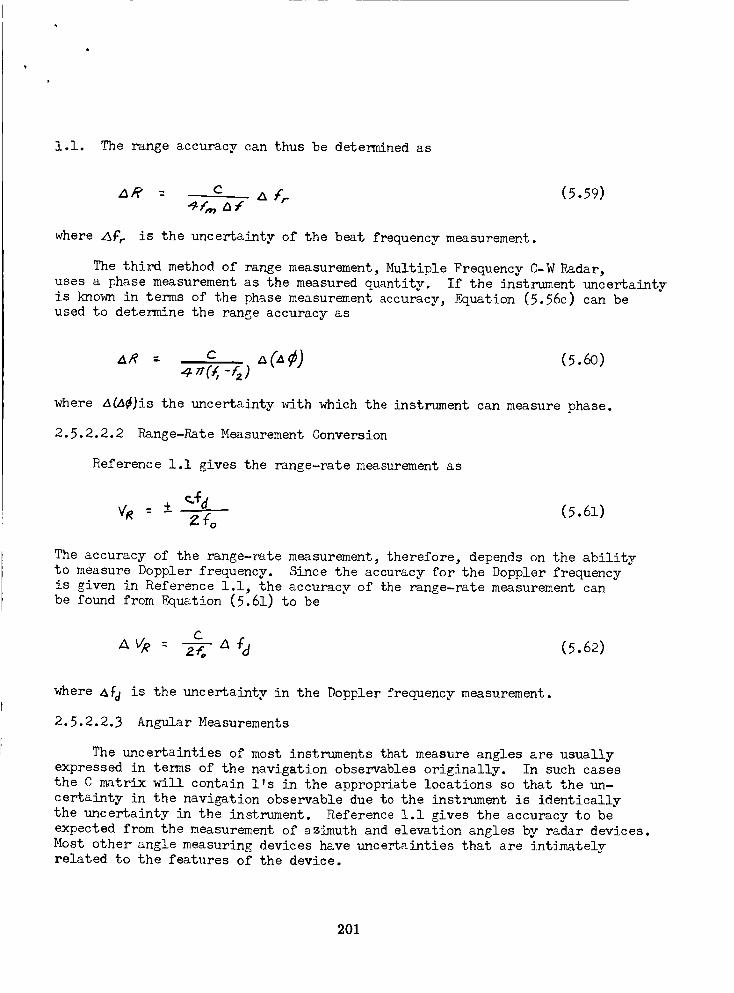
1.1. The range accuracy can thus be detenmined as
where z_ r is the uncertainty of the beat frequency measurement.
The third method of range measurement, Multiple Frequency C-WRadar,
uses a phase measurement as the measured quantity. If the instrument uncertainty
is known in terms of the phase measurement accuracy, F_uation (5.56c) can be
used to deterndne the range accuracy as
where _a¢)is the uncertainty w_th which the instrument can measure phase.
2.5.2.2.2 Range-Rate Measurement Conversion
Reference 1.1 gives the range-rate measurement as
Zfo
The accuracy of the range-r_te measurement, therefore, depends on the ability
to measure Doppler frequency. Since the accuracy for the Doppler frequency
is given in Reference 1.1, the accuracy of the range-rate measurement canbe found from F_quation (5.61) to be
C
where &_ is the uncertainty in the Doppler frequency measurement.
2.5.2.2.3 Angular Measurements
The uncertainties of most instruments that measure angles are usually
expressed in terms of the navigation observables originally. In such cases
the C matrix will contain l's in the appropriate locations so that the un-
certainty in the navigation observable due to the instrument is identically
the uncertainty in the instrument. Reference 1.1 gives the accuracy to be
expected from the measurement of azimuth and elevation angles by radar devices.
Most other angle measuring devices have uncertainties that are int_te_vrelated to the features of the device.
201
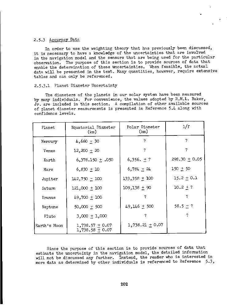
2.5.3 Accuracy Data
In order to use the weighting theory that has previously been discussed,
it is necessary to have a knowledge of the uncertainties that are involved
in the navigation model and the sensors that are being used for the particular
observation. The purpose of this section is to provide sources of data that
enable the determination of these uncertainties. When feasible, the actual
data will be presented in the text. Many quantities, however, require extensive
tables and can only be referenced.
2.5.3.1 Planet Diameter Uncertainty
The diameters of the planets in our solar system have been measured
by many individuals. For convenience, the values adopted by R.M.L. Baker,
Jr. are included in this section. A compilation of other available sources
of planet diameter measurements is presented in Reference 5.A along withconfidence levels.
Plan et
Mercury
Venus
Earth
Mars
Jupiter
Saturn
Uranus
Neptune
Pluto
F_rth's Moon
Equatorial Diameter
A,660 + 30
12,200 + 20
6,378.150 + .050
Polar Diameter
(m)i/f
6,356. + ?
?
?
298.30 + 0.05
6,830 ! i0
IA2,750 + i00
121,000 + i00
A9,700 + lO0
50,000 + 500
3,000 + 1,O00
1,738.57 + 0.07
1,738.58 + 0.07
6,78A _+ 24
133,358 + i00
109,138 + 90
?
A9,1A6 + 500
?
1,738.21 + 0.07
150 + 50
15.2 + 0.im
10.2 + ?
58.5 + ?
Since the purpose of this section is to provide sources of data that
estimate the uncertainty in the navigation model, the detailed information
will not be discussed any further. Instead, the reader who is interested in
more data as determined by other individuals is referenced to Reference 5.3,
202
e
5.5, 5.6, 5.7, 5.8, 5.9, 5.10, 5.11, 5.12, 5.13, 5.1A, and 5.15.
2.5.3.2 Planet Position and Velocity Uncertainty
The uncertainties associated with planet positions and velocities stem
from the fact that the astrodynamical constants of the solar system are
not known accurately. Realizing that the accuracy of these constants will
continually be improved, astronomers decided to "freeze" the values of the
astrodynamical constants in order that an Ephemeris could be written. This
enabled them to construct tables of the planets that matched previousobservations and predicted future observations. The uncertainties in the
constants prohibited the use of standard units in these catalogs, for thevalues would have to be modified each time a constant became known more
accurately. Instead, a system of units that were independent of the uncertain
constants was employed. This gave rise to the use of the astronomical unit.
Although the astronomical unit is not known accurately in terms of conventional
length measurements, it still provides an excellent parameter to describe
the orbital behavior of the planets, because the relative motion of the bodies
in our solar system can be defined very precisely in terms of this unit.
Further, the Ephemeris is independent of the uncertainties of the astrodynamical
constants. For these reasons, the Ephemeris can contain an extremely precise
and self consistent set of data that describes the motion of the planets.
It should be noted that although the data in the Ephemeris is extremely
precise, the accuracy with which it agrees with reality may not be as good.This observation results from the fact that the conversions to conventional
measurements require a knowledge of the constants which are usually not known
as accurately as the precision of the Ephemeris. In particular, the position
of a planet may be known to an uncertainty in the eighth plance in terms of
astronomical units, but the astronomical unit is only known to five places.The uncertainty in position can now be defined in terms of conventional units.
A convenient way to visualize the relationship between the uncertainty
in the astronomical unit and the planet positions is to consider the Ephemeris
as a catalog of the planets that differs from reality by some scale factor.
The scale factor does not change the apparent angular motion of the planets,
but does change their absolute positions and velocities. The uncertainty in
the value of the astronomical unit can be thought of as a change in the scale
of the solar system model. The accuracy of the model to reality depends onthe accuracy of the astronomical unit.
The predicted position of a planet for a navigation observation can be
obtained from the Ephemeris in terms of astronomical units. The uncertainty
in the astronomical unit can then be used in order to find the position
uncertainty. This estimate of the position uncertainty is about the best that
can be achieved with the Ephemeris. If the astronomical unit is someday
known much more accurately, the method of computing the uncertainty from
the Ephemeris will be the same, although the uncertainty will be smaller.
203
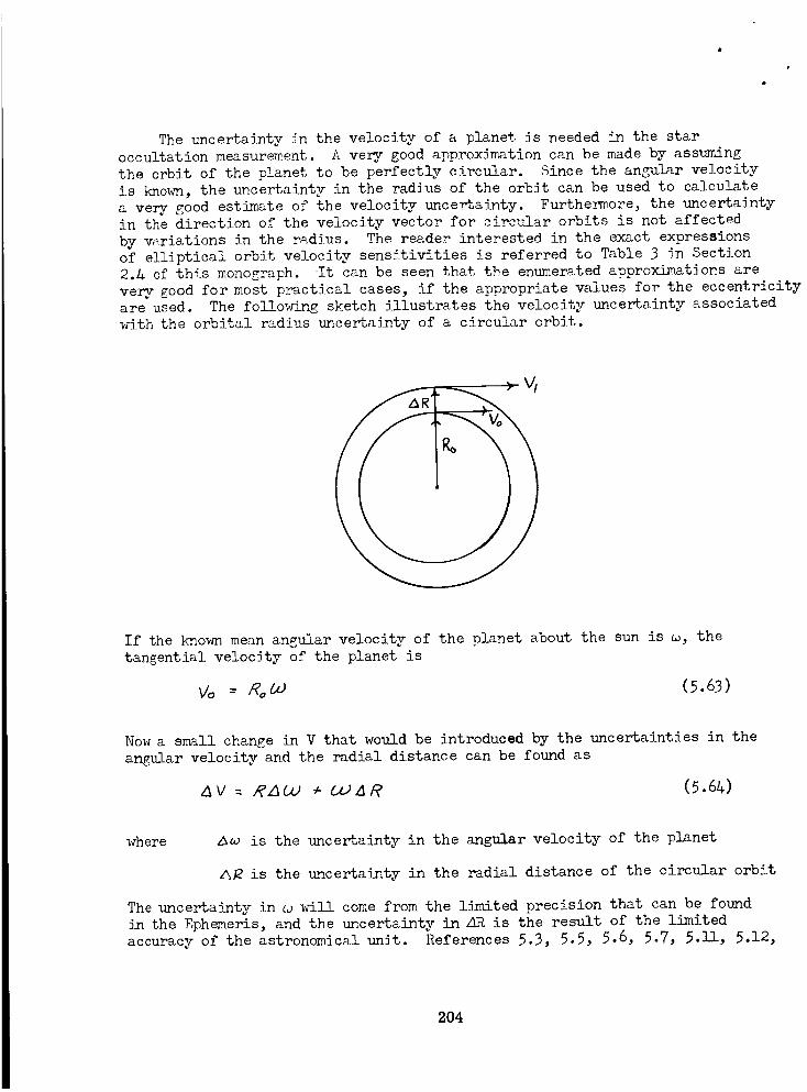
The uncertainty in the velocity of a planet is needed in the star
occultation measurement. A very good approximation can be made by assuming
the orbit of the planet to be perfectly circular. Since the angular velocity
is known, the uncertainty in the radius of the orbit can be used to calculate
a very good estimate of the velocity uncertainty. Furthermore, the uncertaintyin the direction of the velocity vector for circular orbits is not affected
by wriations in the radius. The reader interested in the exact expressions
of elliptical orbit velocity sensitivities is referred to Table 3 in Section
2.A of this monograph. It can be seen that tbe enumerated approximations are
very good for most practical cases, if the appropriate values for the eccentricityare used. The following sketch illustrates the velocity uncertainty associated
with the orbital radius uncertainty of a circular orbit.
vl
If the kno_11 mean angular velocity of the planet about the sun is _, the
tangential velocity of the planet is
Wo --Ro ; (5.63)
Now a sm_ll change in V that would be introduced by the uncertainties in the
angular velocity and the radial distance can be found as
AV = 8_L_ ÷ CU_R (5.64)
where z_ is the uncertainty in the angular velocity of the planet
_ is the uncertainty in the radial distance of the circular orbit
The uncertainty in _ will come from the limited precision that can be found
in the Ephemeris, and the uncertainty in_R is the result of the limited
accuracy of the astronomical unit. References 5.3, 5.5, 5.6, 5.7, 5.11, 5.12,
204
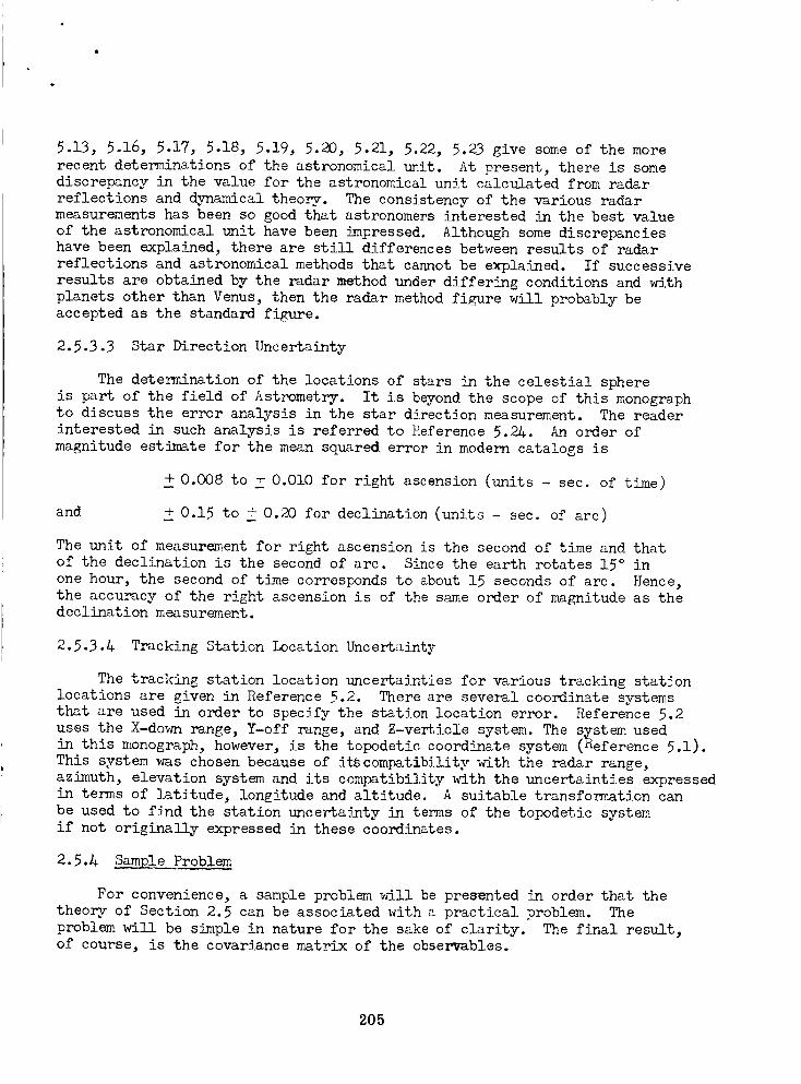
5.13, 5.16, 5.17, 5.18, 5.19, 5.20, 5.21, 5.22, 5.23 give some of the more
recent determinations of the astronomical unit. At present, there is somediscrepancy in the value for the astronomical unit calculated from radar
reflections and dynamical theory. _The consistency of the various radar
measurements has been so good that astronomers interested in the best value
of the astronomical unit have been impressed. Although some discrepancieshave been explained, there are still differences between results of radar
reflections and astronomical methods that cannot be explained. If successive
results are obtained by the radar method under differing conditions and with
planets other than Venus, then the radar method figure will probably be
accepted as the standard figure.
2.5.3.3 Star Direction Uncertainty
The determination of the locations of stars in the celestial sphere
is part of the field of Astrometry. It is beyond the scope of this monographto discuss the error analysis in the star direction measurement. The reader
interested in such analysis is referred to Reference 5.2_. An order of
magnitude estimate for the mean squared error in modern catalogs is
0.008 to _ O.O10 for right ascension (units -sec. of time)
and _ 0.15 to _ 0.20 for declination (units -sec. of arc)
The unit of measurement for right ascension is the second of time and that
of the declination is the second of arc. Since the earth rotates 15 ° in
one hour, the second of time corresponds to about 15 seconds of arc. Hence,
the accuracy of the right ascension is of the same order of magnitude as thedeclination measurement.
2.5.3.& Tracking Station Location Uncertainty
The tracking station location uncertainties for various tracking station
locations are given in Reference 5.2. There are several coordinate systemsthat are used in order to specify the station location error. Reference 5.2
uses the X-down range, Y-off range, and Z-verticle system. The s_stem usedin this monograph, however, is the topodetic coordinate system ( eference 5.1).
This system was chosen because of it_compatibilitywith the radar range,
azimuth, elevation system and its compatibility with the uncertainties expressed
in terms of latitude, longitude and altitude. A suitable transformation can
be used to f_nd the station uncertainty in terms of the topodetic system
if not originally expressed in these coordinates.
2.5.A Sa___ple Problem
For convenience, a sample problem will be presented in order that the
theory of Section 2.5 can be associated with a practical problem. The
problem will be simple in nature for the sake of clarity. The final result,of course, is the covariance matrix of the observables.
205
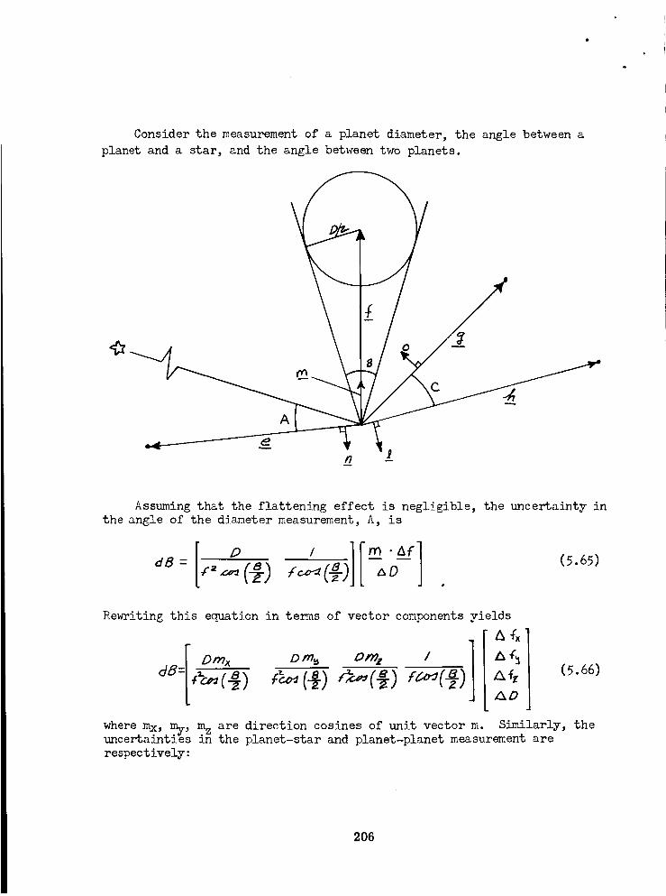
Consider the measurement of a planet diameter, the angle between a
planet and a star, and the angle between two planets.
A
C
Assuming that the flattening effect is negligible, the uncertainty in
the angle of the diameter measurement, A, is
dB = (5.65)
Rewriting this equation in terms of vector components yields
Dm,_ D m_ Dp'_ I ]_D
(5.66)
where mx, my, mz are direction cosines of unit vector m. Similarly, theuncertainties in the planet-star and planet-planet measurement are
respectively:
206
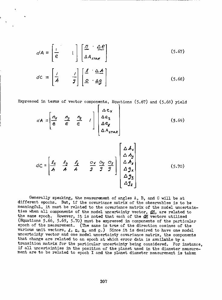
dA =
dC =
(5.67)
(5.68)
Expressed in terms of vector components, Equations (5.67) and (5.68) yield
Z_ w
A%
A A_TAR
(5.69)
[
A,Ax
Zgx(5.70)
Generally speaking, the measurement of angles A, B, and C will be at
different epochs. But, if the covariance matrix of the observables is to be
meaningful, it must be related to the covariancematrixof the model uncertain-
ties when all components of the model uncertainty vector, dM, are related to
the same epoch. However, it is noted that each of the dMvectors utilized
(Equations 5.66, 5.69, 5.70) must be expressed in components of the particular
epoch of the measurement. (The same is true of the direction cosines of the
various unit vectors, _, _, m, and o.) Since it is desired to have one model
uncertainty vector and one model uncertainty covariance matrix, the components
that change are related to an epoch at which error data is available by a
transition matrix for the particular uncertainty being considered. For instance,
if all uncertainties in the position of the planet used in the diameter measure-ment are to be related to epoch I and the planet diameter measurement is taken
207
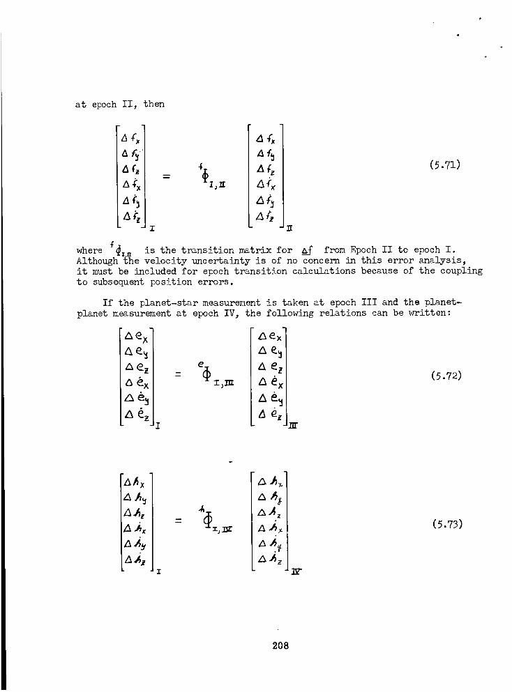
at epoch II, then
'_,"_1
A._,, I
.J"r
m
a-r,
(5.71)
where _._- is the transition matrix for A_ from Epoch II to epoch I.
Although the velocity uncertainty is of no concern in this error analysis,
it must be included for epoch transition calculations because of the coupling
to subsequent position errors.
If the planet-star measurement is taken at epoch III and the planet-
planet measurement at epoch IV,
&e X
ae_l
Z3 e x I)_
A e_
_5 ez
the following relations can be v_itten:
Z_ _×]
A e.,,, I
A _£=,1
Z_ exl (5.72)
A e,,I
t_ e..,i-.]E'
A_x
aAz _.'4z I_!
"1ZX_z
(5.7_)
208
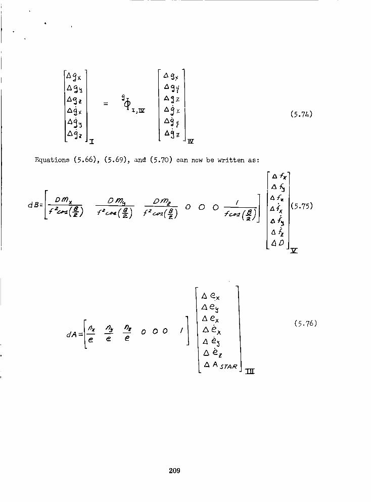
i
- I
F_uations (5.66),
A_z
(5.69), and (5.70) can now be written as:
. o
A_
(5.7_)
(_.75)
Z
d A = [_ _ #_'i _-_t ° 0 0ee I1
A _.x
zl e_
A e x
a e3
/_ A _FARTIT
(5.76)
209
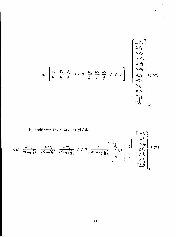
000 °°1 aSx
a2,
(5.77)
11Z
Now combining the notations yields
I 1I
fz_I
I
I _4Z_D
(5.78)
210
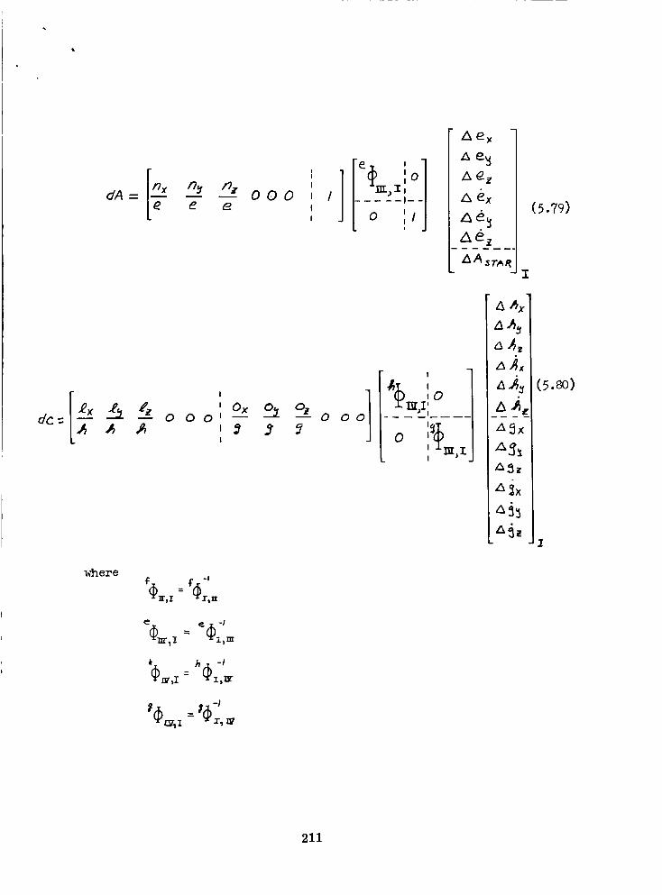
dA =I
!
ZX_ x
ZX e_
ZX_
A &x
,,_&_
AA_TA R
(5.79)
I
]' Ox °_ °, o o o0 0 I --
I
n ,6x
6 A_
max
n A s
A Az
xx_
n _x
a6z
(5._)
I
where
e.. -I
h -I
211
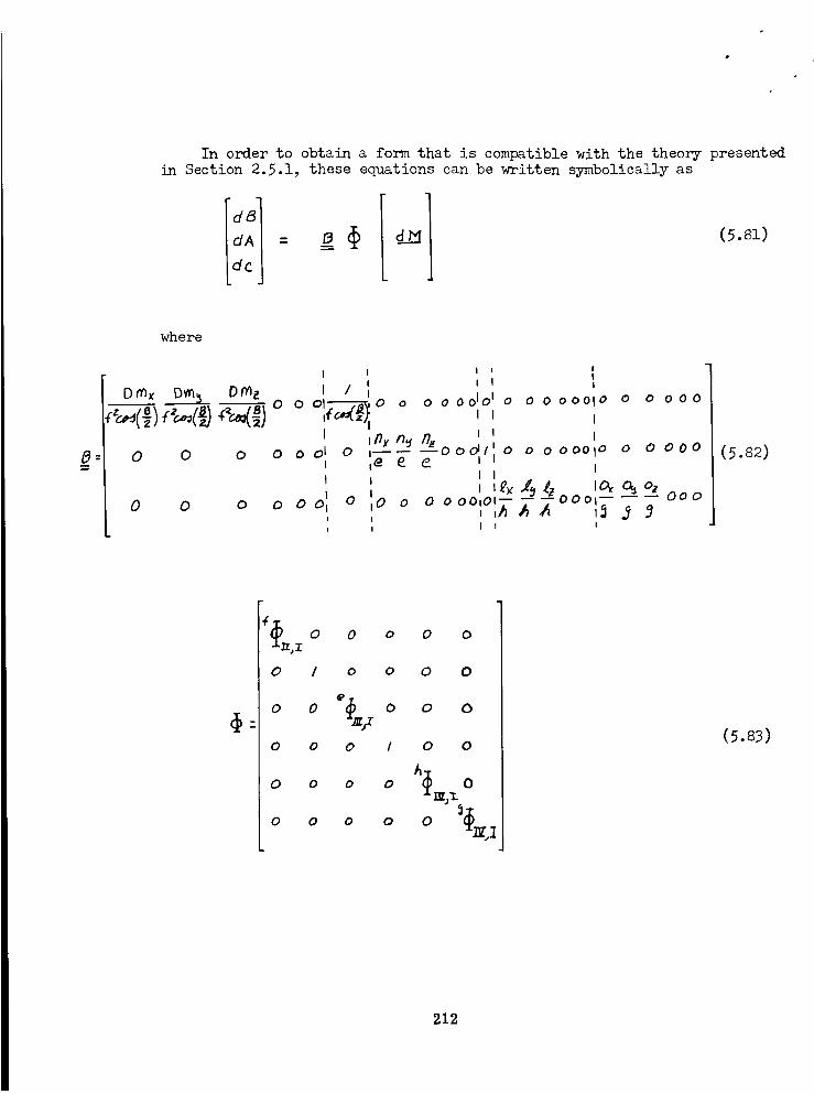
In order to obtain a form that is compatible with the theory presented
in Section 2.5.1, these equations can be written symbolically as
C
(5.81)
where
0 0 o
I tI
I / I
ooo
0 0 o o
o
t
o o I1
0 o Ii
I| = tI I I
0 0 0 00101 0 0 0 000_0 0 0 0 O0I I I
,n_n_ n__oo_ I' I'ioo o 00o,0o o oooo ,y_-_ ,,
I l& J_ tz Io,o_ o_ oooo I _oo _,0 o 0 o oo,0'-- -- °11_- _ _'_,AAA
t
i
(5.82)
f_ 0 0 o 0 o,I
o I o o 0 0
0 0 _/I/T o o 0
o o o / 0 0
/.1
"mj'z.
0 0 0 0 ]
(5.83)
212
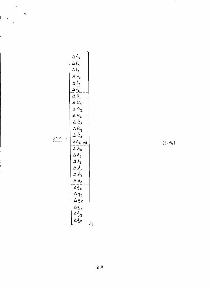
AD
& ex
A e5
i
di____[=A AS-TA R
AA_
6Az
Az
_x
T
(5.8_)
213

It should be noted that manyzeroes are introduced into the matricesin this process at the expenseof space for purposesof illustration of theform of the problem. In an actual mechanization of this problem on a cow,purer,it is moredesirable to perform the computations in parts in order to avoiduseless core storage of zeroes.
Nowthat the covariance matrix of the observables (Z(d__Md_.r)) has
been "frozen" to a particular epoch, the results of Section 2.5.1 can be
applied to deterv_ne the covariance matrix of observables to be
Note should be made that the previous results simplify if the three measure-
ments are taken close enough in time to be considered simultaneous. If dN
is known during the epoch of the three measurements, then
=I (the identity matrix)
and then
where _ and _ h_ve been defined previously.
Since the measure_,ent made in this sample problem are angles, it is
not necessar_ to convert the measurements to navigation observables. Hence,the covariance matrix of the instrtunent inaccuracies can be added to the
result of Equation (5.86) in order to obtain the total covariance due tothe model and instrument uncertainties.
214
3.0 RECO_NDED PROCEDURES
The discussions presented within the state-of-the-art review present
several variations of the means which may be employed to obtain initial esti-
mates of the orbit and subsequently improve these estimates through data
smoothing. Thus, it is desirable to suggest specific applications for this
material or conversely recommend combinations of these techniques for problemsof common interest.
The initial fix on the trajectory as was shown can be accomplished in
several distinctly different means depending on the data available. Thesemethods are summarized in Table 3.1.
However, as was discussed, there is a distinct chance for non-negligible
error in the initial orbit if raw data are employed in the process. Rather,
it was shown in Section 2.1.A that a series of preliminary operations should
be performed to eliminate biases and random scatter in the data resulting
from errors in the observation process, the mathematical model, and the instru-
ment employed for the measurement.
The developments then turn to means of improving knowledge of the initial
orbit and including the affects of perturbing accelerations. In particular,
three types of estimators are developed:
least squares
weighted least squares
minimum variance (recursive and non-recursive)
are developed from simple concepts of "loss" or "optimality" of the fit.
Subsequent developments then addressed themselves to the task of explaining
the basic estimation problem, the mechanism in which the statistics of the
errors, non-linear estimation techniques and/or non-linear dynamics might be
introduced to the problem, and the equivalence of the estimators previously
developed under certain assumptions regarding the statistics of the data. It
was in this latter discussion where the concept of sufficient statistics was
introduced and there it was shown that, in general, the Bayes estimator was
superior to others which might be developed. It was also in this latter dis-cussion that it was shown that the minimum variance biased estimator (_.[_Bor
Kalman) was a Bayes estimator where the statistics are Gaussian and where the
loss function is simple.
Since the set of assumptions utilized in developing the MVB estimator
closely corresponds to the nature of __mostorbit determination problems, it is
recommended that the MVB estimator of the form developed in Sections 2.2.2.&
and 2.2.2.5 be applied. Care must be exercised, however, to confirm for any
215
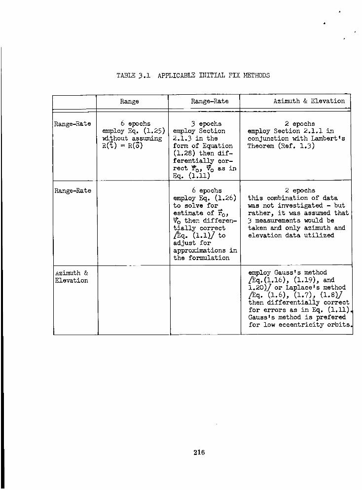
TABLE 3.1 APPLICABLE I_ITIAL FIX METHODS
Range-Rate
Range-Rate
Azimuth &
Elevation
Range
6 epochs
employ Eq. (1.25)
without assuming
R(_) = R(_)
Range-Rate
3 epochs
employ Section
2.1.3 in the
form of Equation
(1.28) then dif-
ferentially cor-
rect_o, To as in
Eq. (i. ii)
Azimuth & Elevation
2 epochs
employ Section 2.1.1 in
conjunction with Lambert'sTheorem (Ref. 1.3)
2 epochsthis combination of data
was not investigated - but
rather, it was assumed that
3 measurements would be
taken and only azimuth andelevation data utilized
6 epochs
employ Eq. (1.26)to solve for
estimate of r_o,
V_o then differen-
tially correct
fEq. (1.1).7 to
adjust for
approximations inthe formulation
employ Gauss's method
fEq.(1.16), (1.19), and
1.20)g or Laplace's method
EEq. (1.6), (1.7), (l.8)J
then differentially correct
for errors as in Eq. (i.ii)
Gaussls method is prefered
for low eccentricity orbits
216
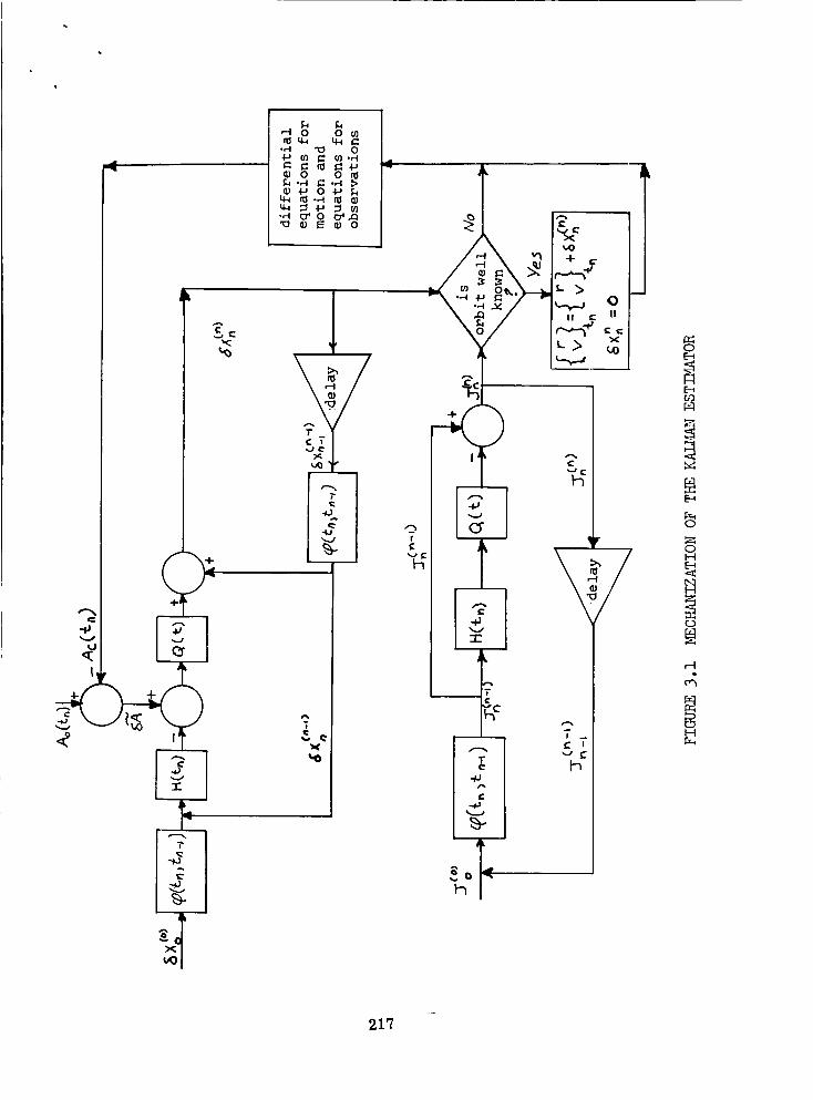
_1 0 0 r__q._ q-I _
,,-I "_ 0
• 0 O_ _°,_
q_ _-_ _ _
-I"
p
!
xuO
J
C
tO
I'
"-A "_ _ _"'/--_
r_+ _
t> t_
+
8
II '_7
h
t'n
/
0
O
OI-4
r_
r--I
I--t
217
given application that the use of this estimator is justified. If not, an
alogrithm must be developed from the Bayes formulation for that specific
application. This test will not, in general, be easily performed; however,
should the statistics of the problem be sufficiently different from those used
in developing the _B, the results could differ to a large degree. There is,
however, one means of applying the MVB so that the results will be approxi-
mately correct if the number of error sources is large. This means existsdue to the central limit theorem of statistics which states that the distribu-
tion of a function of random variables approaches Gaussian as the number of
variables increases. Thus, a Gaussian model can be constructed which will be
equivalent to the more precise process.
The mechanization of Kalman's form of the minimum variance estimator is
shown in Figure 3.1. This procedure is preferred above other _B estimators
because of the fact that it provides for the utilization of initial data
regarding the state of the system and because it is recursive (to minimize
estimation problems and to provide a means of limiting the assumed duration
for linear expansion about the nominal trajectory). One source of trouble may
exist in that the procedure illustrated for updating the matrix J involves
differencing. If J ever approaches the null matrix, it is thus possible for
one of the eigen values of the updated matrix to be negative (due to roundoff,
loss of numerical significance, etc.). Thus, for these cases, J should be
updated in the manner specified in Equation (2.77).
Attention is drawn specifically to the decision function illustrated in
the lower right-hand corner of the previous figure. A simple test is made to
determine if the covariance matrix for the estimation errors is sufficiently
small to allow the estimated state to be added to the reference trajectory so
that future computations can employ a more precise reference. One such test
consists of comparing the summation of the terms along the diagonal of J (or
its diagonal equivalent, Appendix C) to a comparison function constructed to
define _u acceptable re&ion (6 dimensions) for errors in the radius and veloc-
ity vectors. (For example,
F/
Attention then turns to the development of the state transition matrix
for perturbed and conic motions. This material is intended to provide the
user with a series of tools which can be applied to achieve a level of accuracy
adequate for his needs. This objective is accomplished by approximating the
true trajectory (for the purposes of constructing the transition matrix only)
with a series of aonic arcs, as described in Section 2._.2.3, and by employing
an analytic inverse property which is developed for this matrix.
The covariance matrix for the errors in the observables is constructed as
the final major step in the presentation. This development relates the affects
of navigation model uncertainbies and sensor errors on the observables being
processed for the purpose of providing the navigational filter with data
required to weight the observed minus computed residuals. This step is accom-
plished by constructing the linear relationships between the errors in theobservables and the errors in the model itself for each of the navigational
218
techniques discussed in Reference I.i. These partial derivatives are then
utilized in conjunction with error data for constants of the model (assumed
to be normally distributed) to construct the desired covariancematrix. This
procedure, _nile not always precise (due to non-Gaussion errors, etc.) is
recommended for all cases in which more accurate data are not available.
The monograph concludes with a series of appendices which are designed
to provide a background in the most normally applied statistical procedures.
This material leads to the development of the concept of an error volume and
the assignment of a probability of enclosure within the volume, thus allowing
the covariance matrix for estimation errors (Sections 2.2 and 2.3) to be
interpreted geometrically. This fact is particularly useful in discussingthe results of a specific analysis.
219
4.0 REFERENCES
O.1
0.2
o.3
0.4
0.5
0.6
0.7
0.8
0.9
Kalman, R. E. "A New Approach to Linear Filtering and Prediction
Problems," Journal of Basic Engineering. PP. 35-45 (March 1960).
Schm_dt, S. F., et al. Application of Statistical Filter Theory to the
Optimal Estimation of Position and Velocity on Board a CircumlunarVehicle. NASA, TR-R135 (1962).
Battin, R. H. "A Statistical Optimizing Procedure for Space Flight,"
ARS Journal. Vol. 32, No. ll, pp. 1681-1696 (November 1962).
Middleton, D. Statistical Communications Theory. New York: McGraw-
Hill Book Company (1960).
Marshall, W. C. The Adjoint Method and Some Applications to Astronautics.
llinneapolis-Honeywell }IPG Document, U-RD-6171 (October 1961).
Danby, J. M. A. "Matrix Methods in the Calculation and Analysis of
Orbits," AIAA Journal. Vol. 2, No. l, pp. 13-19 (January 1964).
Kochi, K. C. "Exact Two-Body Error Sensitivity Coefficients," AIAA
Journal. Vol. 2, No. 8, pp. 1502-1504 (August 1964).
DeVries, J. P. "Elliptic Elements in Terms of Small Increments of
Position and Velocity Components," AIAA Journal. Vol. l, No. ll,
pp. 2626-z629 (November 1963).
Townsend, G.E. "The State Transition Matrix for Conic Motion,"The Differential Corrections Geocentric Orbit Computation Program.
1.1
NAA S&ID, SID 65-1203-1, pp. 288-306 (January 1966).
F_ller, B. J. and Abbott, A. S. Observation Theory and Sensors. NAA
S&ID, SID 65-1200-2 (December 1965).
1.2 Townsend, G. E. Differential Corrections Geocentric Orbit Computation
1.3
1.4
1.5
Program. NAA S&ID, SID 65-1203-1, pp. 239-241 (January 1966).
Townsend, G. E. and Tamburro, M. B. The Two-Body Problen% NAA S&ID,
SID 65-1200-3 (February 1966).
Danby, J. M. A. Fundamentals of Celestial Mechanics. The MacMillan
Company: New York, pp. 169-172, pp. 146-148, pp. 177-18_ (1962).
Herget, P. The Computations of Orbits. University of Cincinnati,
published bythe author (1948).
220
3.1 Mood, A. M. Introduction to th e Theory of Statistics. 2nd Edition.
New York: McGraw-Hill Book Company (1963).
3.2 Uspensky, J.V. Introduction to Mathematical Probability. New York:McGraw-Hill Book Company(1937).
4.1 Kraft, J.D. "Orbit Computation," The Orbital Flight Handbook.NASA, SP-33 (1962).
5.1 Tamburro, M. B., Abbott, A. S., and Townsend, G. E. Coordinate Systems
and Time _asure. NAA S&ID, SID 65-1200-1 (October 1965),
5.2 Mann, H. P. The Accuracy of AMR Instrumentation. Air Force Missile Test
Center, Patrick Air Force Base, Florida, Technical Documentary ReportNo. _C-TDR-64-1 (December 1963).
5.3 Makemson, M. W., Baker, R. M. L., and _stron, G. B. "Analysis and
Standardization of Astrodynamic Constants," Astronautical Journal.
Vol. VII, No. 1 (Spring 1961).
5.4 Townsend, G. E. and Kraft, J. D. Space Flight Handbooks. 3 Volumes.
The _rtin Company, Space Systems Division, Baltimore, Maryland, NASA,
N63-21101 (1963).
5.5 _cDonald, G. J. F. "Radar Studies of the Planets," Reviews of Geophysic S.Vol. 2 (November 1964).
5.6 Notes of Workin_ Symposium on Solar System Constants. Rand Corporation,
_ 3525, NASA Reproduction No. N63-18371 (May 1963).
5.7 Herrick, S._Baker, Jr., R. M. L. and Hilton, C. G. "Gravitational and
Related Constants for Accurate Space Navigation," UCLA AstronomicalPa__. Vol. i, No. 14 (1958).
5.8 Kuiper, G. P. "The Diameter of Neptune," Astrophysics Journal. p. lO(1949); "The Diameter of Pluto," Pub. A.S.P. p. 62 (1950).
5.9 Reuyl, D. "Photographic Determination of the Diameter of Mars,"
Astronomical Journal. P. 49 (1941).
5.10 Van de Kamp, P. "A Determination of the Diameter of Mars," Astronomical
Journal. p. 38 (1928).
5.11 Allen, C.W. Astrophysical Quantities. University of London: The
Athlone Press (1955).
5.12 Clemence, G.M. "On the System of Astronomical Constants," Astronomical
Journal. Vol. 53, P. 178 (1947).
5.13 De Sitter, W. "On the System of Astronautical Constants," Bulletin ofthe Astronomical Institute of Netherlands VIII. pp. 213-231 (July 1938).
221
5-]/+ Victor, W. K., Stevens, R. and Golomb,S. W. Radar Explorations of Venus
JPL, TR 32-131 (August 1961).
5.15 Pettingill, G. H., et al. "A Radar Investigation of Venus," Astronomical
Journal. p. 67 (May 1962).
5.!6 ,'Coordinates of Venus," AstronoL_ical Papers. Vol. 15, Part 3, Nautical
Almanac Office, U. S. Naval Observatory, GPO, Washington D.C. (1955).
5.17 Duncombe, R. L. "Motion of Venus," Astronomical Papers. Vol. 16, Part l,
Nautical Almanac Office, U. S. Naval Observatory, G.P.O., Washington, D.C.
(1958).
5.18 Newcomb, S. "Tables of the Motion of the Earth on Its Axis and Around
the Sun," Astronomical Papers. Vol. 6, Part l, Nautical Almanac Office,
U. S. Naval Observatory, G.P.O., Washington, D.C. (1898).
5.19 Newcomb, S. "Tables of the Heliocentric Motion of Nmrs," Astronomical
Pa__. Vol. 6, Part &, Nautical Almanac Office, U.S. Naval Observatory,
G.P.O., Washington D.C. (1898).
5.20 Staff, Nillstone Radar Observatory, Lincoln Laboratory, MIT, "The Scale
of the Solar System," Nature. Vol. 190, p. 592 (_y 13, 1961).
5.21 Block, N. Computation of Lunar Positions from the Improved Brown Lunar
The___. JPL, Research Summary 36-12, Vol. l, pp. 125-128
(January 1962).
5.22 Muhlemsm, D. 0., Holdridge, D. B. and Block N. The Astronomical Unit
Determined by Radar Reflections from Venus. JPL Technical Report,No. 32-221 (_rch 1962).
5.23 Thompson, J. H., et al. "A New Determination of the Solar Paralax by
Means of Radar Echoes from Venus," Nature. pp. 1950-1959 (l_ay 1961).
5.2& Podobed, V. V. Fundamental Astrometry. Chicago: University of Chicago
Press (1962).
222
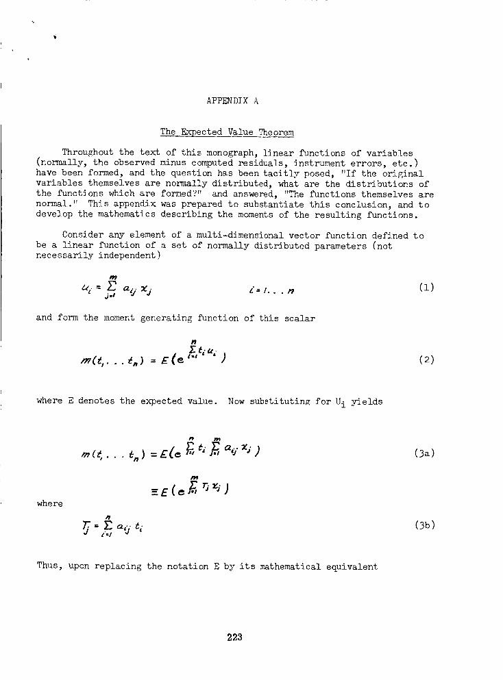
APPENDIXA
The Expected Value Theorem
Throughout the text of this monograph, linear functions of variables
(normally, the observed minus computed residuals, instrument errors, etc.)
have been formed, and the question has been tacitly posed, "If the original
variables themselves are normally distributed, what are the distributions of
the functions which are formed?" and answered, "The functions themselves are
normal." This appendix was prepared to substantiate this conclusion, and to
develop the mathematics describing the moments of the resulting functions.
Consider any element of a multi-dimensional vector function defined to
be a linear function of a set of normally distributed parameters (not
necessarily independent)
m
J-, ae. zj. (-'= /...n (I)
and form the moment generating function of this scalar
_(_,... _,) : L-(e _,t,._; ) (2)
where E denotes the expected value. Now substitutin_ for Ui yields
where
WyS
= E .-,,).tic"=/
(3a)
(3b)
Thus, upon replacing the notation E by its mathematical equivalent
223
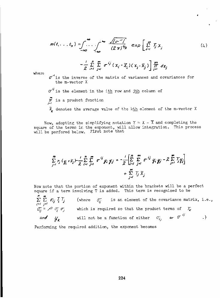
.,,,...,.,--j=../-r
C2 _')'_ j.,
where
. ]2. ,'.1 ./-I
_-lis the inverse of the matrix of variances and covariances for
the m-vector X
G -'j is the element in the it__hrow and jth column of
is a product function
_ denotes the average value of the kt__hhelement of the m-vector X
Now, adopting the simplifying notation Y = X - X and completing the
square of the terms in the exponent, will allow integration. This process
will be perfored below. First note that
Inm (i
j'-Ii=I j =/ ,J-_
+ s r.._:j=/
Now note that the portion of exponent within the brackets will be a perfect
square if a term involving T is added. This term is recognized to be
n
Z'=/ j,l
Q_m/ _ will not be a function of either q_) or [7"
Performing the required addition, the exponent becomes
(where _ is an element of the covariance matrix, i.e.,
which is required so that the product terms of
.)
224
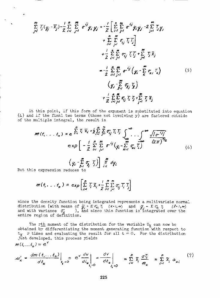
rn I n m
J=/ _z::_ o- y,.,,0i-I ,j=lI wI-; ;?,
Z'=/ j=l
/ _ m m
_-I j-I
I Z' a-'J2 ,':1ja J4" %
j ,,em m
¢'=1j=i
(5)
At this point, if this form of the exponent is substituted into equation
(_) and if the final two terms (those not involving y) are factored outside
of the multiple integral, the result is
... j.,%.7; U =o• = =
-oO
_×p -_. x r. o-'_ _ _.r_)d=/ j=_ =(6)
But this expression reduces to
_,1 " .j,I
since the density function being integrated represents a multivariate normal
distribution (with means of _ : _ (_=l,m) and _j- Z_j _ (J:/,_)
and with variance _ ), and since this function is mn_egrated over the
entire region of definition.
The rthh moment of the distribution for the variable UK can now be
obtained by differentiating the moment generating function with respect to
t K r times and evaluating the result for all t = O. For the distribution
just developed, this process _vieldsV
(7)
225
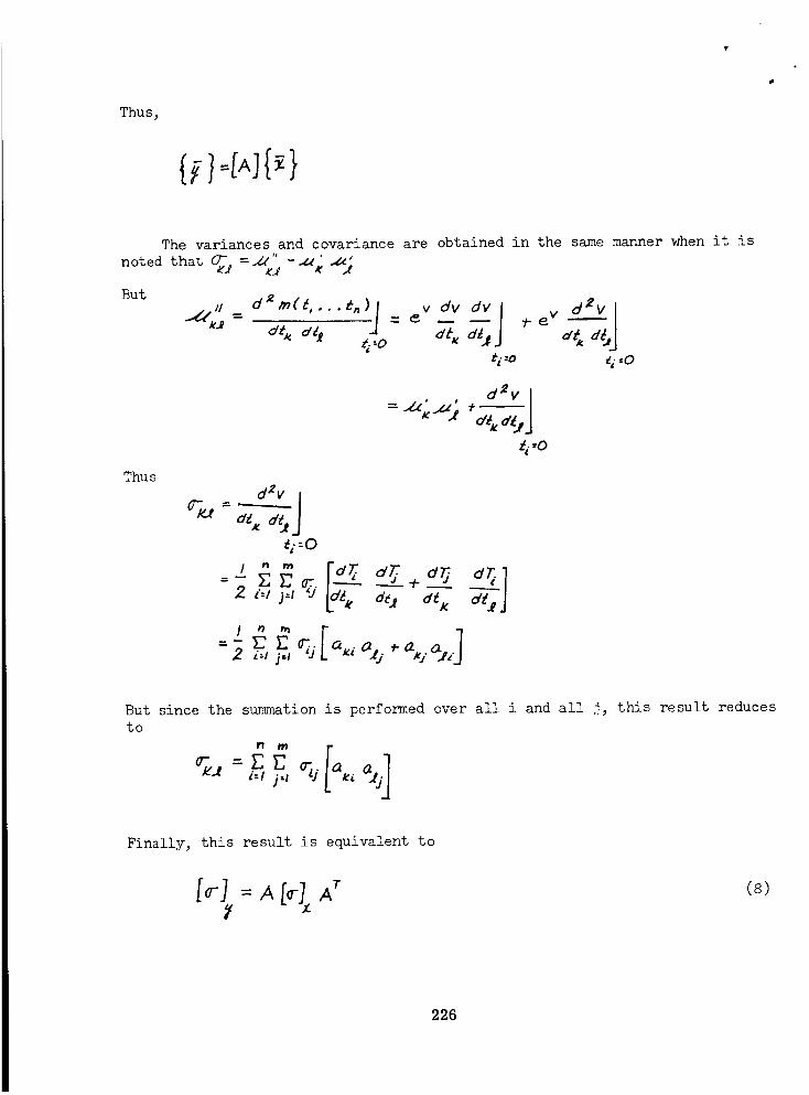
Thu s,
{/l+J{
The variances and covariance are obtained in the same manner when it is
noted that O_i--_" -_ _
But
_i-'o _i --o
Thus
d_v I
li--O
_i--oI
[%' #-_-_#'x d£,
j2 i:; i._
But since the summation is performed over all i and all j, this result reducesto
i_'l j'-I O"_j It.i
Finally, this result is equivalent to
[_-]: A[_-]_A_ (a)
226
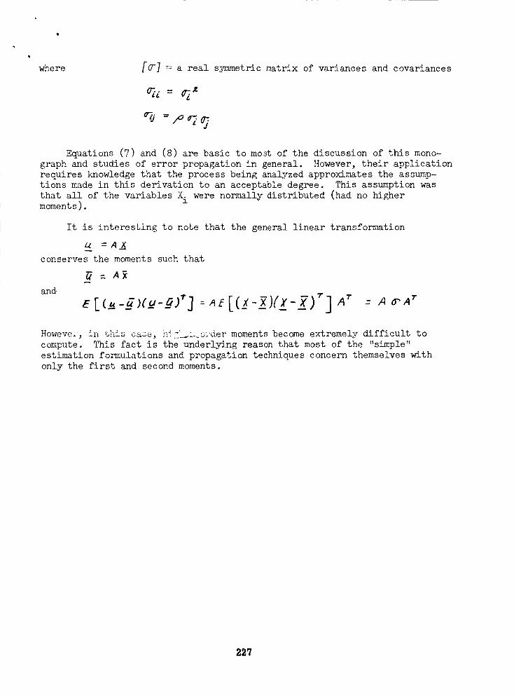
where [G'] = a real symmetric matrix of variances and covariances
Equations (7) and (8) are basic to most of the discussion of this mono-
graph and studies of error propagation in general. However, their application
requires _uowledge that the process being analyzed approximates the assump-
tions made in this derivation to an acceptable degree. This assumption was
that all of the variables X. were normally distributed (had no higherl
moment s).
It is interesting to note that the general linear transformation
= A
conserves the moments such that
an_
: A" = A_"A T
However, in this cacc, hi::_:_:_o:'der moments become extremely difficult to
compute. This fact is the underlying reason that most of the "simple"
estimation formulations and propagation technie_es concern themselves with
only the first and second moments.
227
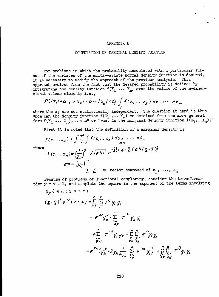
m
APPENDIX B
CO_._UTATION OF MARGINAL DENSITY FUNCTION
For problems in which the probability associated with a particular sub-set of the variates of the multi-variate normal density function is desired,
it is necessary to modify the approach of the previous analysis. This
approach evolves from the fact that the desired probability is defined by
integrating the density function f(X 1 ... Xm) over the volume of the m-dimen-
sional volume element; i.e.,
zs)d , ...P(/_,l_ ,
V
where the x i are not statistically independent. The question at hand is thus"how can the density function f(X I ... _) be obtained from the more general
form f(X I ... _), n > m" or "what is th'_ marginal density function f(XI...Z_)."
First it is noted that the defi_&tion of a marginal density is
2_. 2f(x-,..._h,) - _" F(Z,...Z_) dz:4 • • • dZ,m÷l
where I 3 -_[( r.- _)rO=*iJ( Z -,_, ).7
z,,) = ....-I
_-_ --K = vector composed of Xl, ..., x n
Because of problems of functional complexity, consider the transforma-
tion y =x -___ and complete the square in the exponent of the terms involving
n n
L=I j-l
n _g
n £$c' n n
i:l g_'f_ Z"I J'-'l
I_gl 2 I nn n _j
d*l "*1#X J_K
228
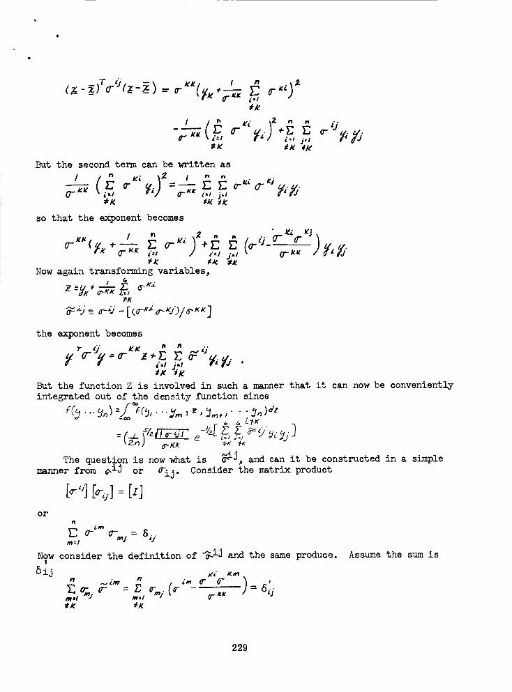
/_g I n 2
(z-Wg')cz-_) = ,,- (f_÷7-_ r r")i-O
";-_ _- _,. .,:, 3._o-_.j,U
But the second term can be written as
/(_O._i) 2t KA
so that the exponent becomes
/ n 2 . ' k'Z_k'i_
Now again transforming variables,
t ,_ d.K;
_K
the exponent becomes
r(7- = .0"
_':1 j;_#X
But the function Z is involved in such a manner that it can now be conveniently
integrated out of the density function since
e(_..._o_--_c_,..._,_,,, _,,... _o_,- _ _ L_
J=l dr. _J"
k2_) _.KX -+K ,K
The question is now what is _ij and can it be constructed in a simple
manner from _iJ or 0_i3. Consider the matrix product
[_')I[_,j]=[dor
n
C o-- o-_= S,.jm=l
Now consider the definition of _ij and the same produce.;
...,._ n ,._, ¢ ¢- ) _:).Z%.r = z %.(r - =m_l _zl ft.. £K
•_R #It
Assume the sum is
229
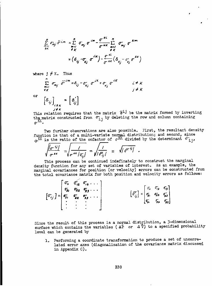
n ,m a"_; h Km
where J # K. Thus
E _y ¢" =_-.-
_K
or
3¢KThis relation requires that the matrix s£j be the matrix formed by inverting
the matrix constructed from o-ij by deleting the row and column containingO_Y_ .
Two further observations are also possible. First, the resultant density
function is that of a multi-variate normal distribution; and second, since
_KK is the ratio of the cofactor of _KK divided by the determinant _ij'
- "I .I- =This process can be continued indefinately to construct the marginal
density function for any set of variables of interest. As an example, the
marginal covariances for position (or velocity) errors can be constructed from
the total covariance matrix for both position and velocity errors as follows:
_15 ° ° •
.I
Since the result of this process is a normal distribution, a 3-dimensional
surface which contains the variables ( A_ or A_) to a specified probability
level can be generated by
le Performing a coordinate transformation to produce a set of uncorre-
lated error axes (diagonalization of the eovariance matrix discussed
in Appendix C).
23O
2. Integrating the resultant distribution (Appendix C) to evaluate the
radius of the equivalent sphere.
3. Using the radius of the equivalent sphere as a constraint on the
values, which can be attained by the variables measured along the
three principal axes, generate the 3-D ellipsoid.
4. Transforming the coordinate system to construct the error ellipsoidin the desired coordinate system.
231
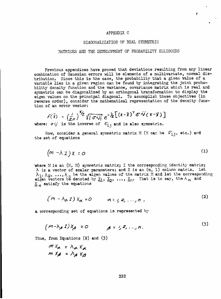
f
APPEt_DIX C
DIAGONALIZATION OF REAL SIq,S_ETRIC
MATRICES AND THE DEVELOPME_r OF PROBABILITY ELLISOIDS
Previous appendices have proved that deviations resulting from any linear
combination of Gaussian errors will be elements of a multivariate, normal dis-
tribution. Since this is the case, the probability that a given value of a
variable lies in a given region can be found by integrating the joint proba-
bility density function and the variance, covariance matrix which is real and
synmetric can be diagonalized by an orthogonal transformation to display the
eigen values on the principal diagonal. To accomplish these objectives (in
reverse order), consider the mathematical representation of the density func-
tion of an error vector:
]where: 0-/j is the inverse of 6_ij and is also symmetric.
Now, consider a general symmetric matrix M (M can be _ij, etc.) andthe set of equations
(_ -Az)x -o (1)
where M is an (M, M) s_Tmnetric matrix; I the corresponding identity matrix;
A is a vector of scalar parameters; and X is an (m, l) column matrix. Let
_l, I\2, ..., _ n be the eigen values of the matrix M and let the corresponding
eigen vectors be denoted by X_l, X_2, ..., X_n. That is to say, the Z_ and
X _ satisfy the equations
a corresponding set of equations is represented by
(2)
Thus, from _,q_tions (2) and (3)
(3)
232
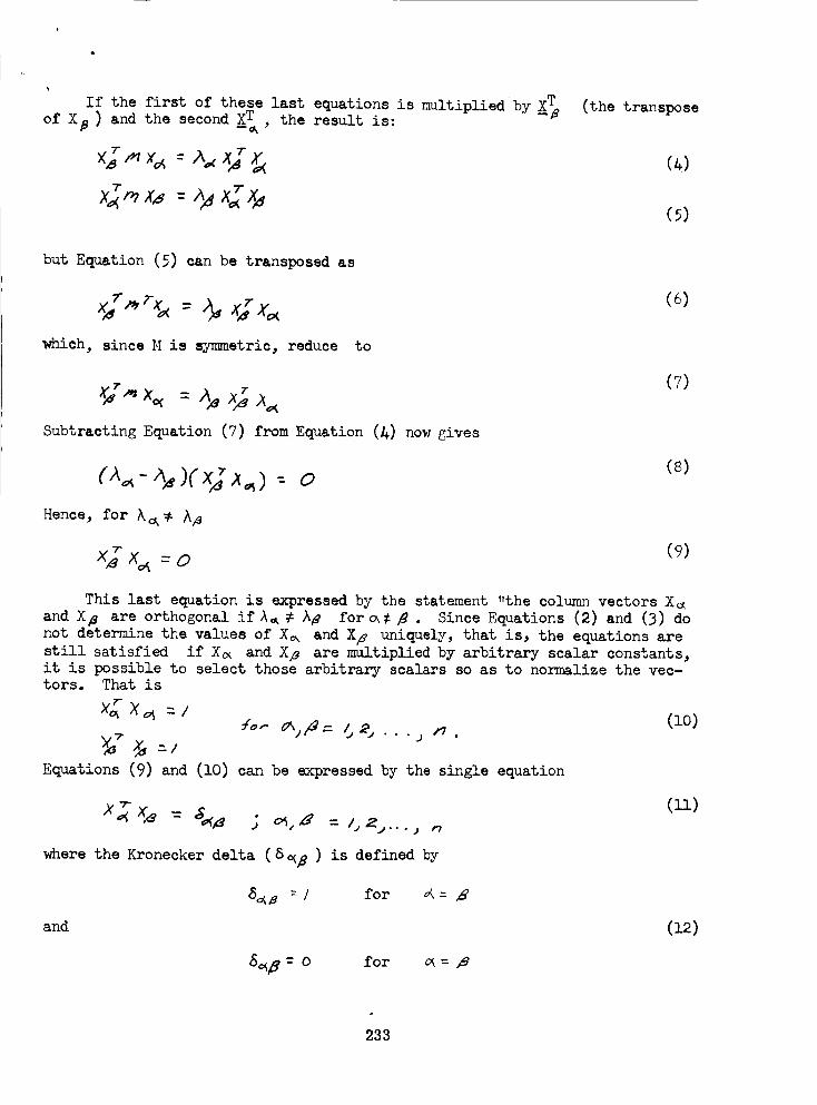
If the first of these last equations is multiplied by X_of X_ ) and the second XT the result is:
(the transpose
(5)
but Equation (5) can be transposed as
which, since M is symmetric, reduce to
(6)
Subtracting Equation (7) from Equation (4) now gives
(7)
Hence, for _ /_A
O(8)
--o (9)
This last equation is expressed by the statement "the column vectors X_
and X_ are orthogonal if A_ _ Ag for _# _ . Since Equations (2) and (3) do
not determine the values of X_ and X/_ uniquely, that is, the equations are
still satisfied if Xm and Xp are multiplied by arbitrary scalar constants,
it is possible to select those arbitrary scalars so as to normalize the vec-tors. That is
_I X_ = / (lO)
Equations (9) and (lO) can be expressed by the single equation
-2"
where the Kronecker delta (6 _B ) is defined by
8_e = I for _<--
and (12)
6_= O for _= ;9
233
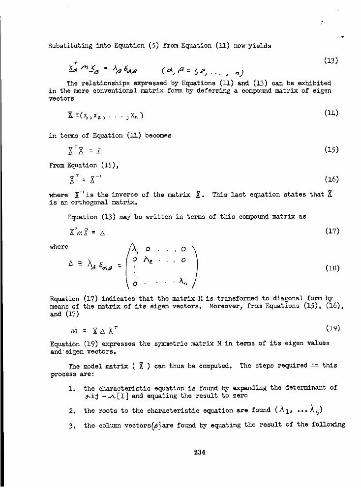
Substituting into Equation (5) from Equation (ll) now yields
(13)
The relationships expressed by Equations (ll) and (13) can be exhibited
in the more conventional matrix form by deferring a compound matrix of eigen
vectors
(_)
in terms of Equation (ll) becomes
X_X = I
From Equation (15),
XT= _,
where X-' is the inverse of the matrix
is an orthogonal matrix•
X •
(15)
(16)
This last equation states that
Equation (13) may be written in terms of this compound matrix as
(17)
i:,oo1o: (i_)
Equation (17) indicates that the matrix M is transformed to diagonal form by
means of the matrix of its eigen vectors. Moreover, from Equations (15), (16),
and (17)
Equation (19) expresses the symmetric matrix M in terms of its eigen values
and eigen vectors.
The model matrix ( _ ) can thus be computed. The steps required in this
process are:
1. the characteristic equation is found by expanding the determinant of
_iJ --_[I] and equating the result to zero
2. the roots to the characteristic equation are found (_l, "'" _ 6)
3. the column vectors{_]are found by equating the result of the following
234
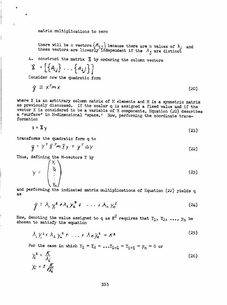
matrix multiplications to zero
there will be _ zj_n vectors _. because there are n values of _j
these vectors are linearly zndependent if the Aj are distinct
A. construct the matrix E by ordering the column vectors
Consider now the quadratic form
and
where X is an arbitrary column matrix of M elements and M is a symmetric matrix
as previously discussed. If the scalar q is assigned a fixed value and if the
vector X is considered to be a variable of M components, Equation (20) describes
a "surface" inM-dimensional "space." Now, performing the coordinate trans-formation
transforms the quadratic form q to
_, _ yT _ 7,__>, : ),T ay (22)
Thus, defining the M-vectors Y by
y _ Y_ (23)
and performing the indicated matrix multiplications of Equation (22) yields q
as
Now, denoting the value assigned to q as K2 requires that YI, Y2, •.., Yn be
chosen to satisfy the equation
J-...,(25)
For the case in which Y1 = Y2 =
/<
•"Yi-I = Yi+l =Yn=O or
(26)
235
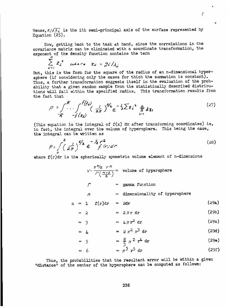
Hence, K/_ is the ith semi-principal axis of the surface represented by
Equation (25).
Now, getting back to the task at hand, since the correlations in the
covariance matrix can be eliminated with a coordinate transformation, the
exponent of the density function contains the termI?
g=/
But, this is the form for the square of the radius of an n-d_ensional h_-ger-
sphere (if considering only the cases for thich the summation is constant).
Thus, a further transformation suggests itself in the evaluation of the prob-
ability that a given random sample from the statistically described distribu-
tions will fall within the specified radius. This transformation results from
the fact that
P = "'" '
-/< -i
(This equation is the integral of f(x) dx after transforming coordinates) is,
in fact, the integral over the volume of hypersphere. This being the case,
the integral can be written as
k
where f(r)dr is the spherically symmetric volume element of n-dimensions
_n/z rn- volume of hypersphere
p = gamma function
n = dimensionality of hypersphere
n = 1 f(r)dr = 2dr (29a)
= 2 = 2Hr dr (29b)
= 3 = _r 2 dr (29c)
= _ = 2 _2 _ dr (29d)
= 5 = _ _2 r_ dr (29e)3
= 6 = _3 r 5 dr (29f)
Thus, the probabilities that the resultant error will be within a given
"distance" of the center of the hypersphere can be computed as follows:
236
where erf(K) denotes the error function.
Numerical data are tabulated for these six cases as a function of the
radius, K, in Table C.1.
237
II oo_008880
,.0 D+-¢r_ _0',0"_ _0 r-I
_oooR_er_ u'_-,¢,-_r--
C_ o"_-.C)D-- u'_
OtOQQ
Lr_..O 0r-I u"_O00.,,0-,0 _.0". 0",0",
H0 L_ ur',I_O
O00C'_8oO8oQ • Q •
_H_O_0_
O _e_tQe
•...¢ cr_ O_ 0 ,--I0 .-_" 00W u'xu'x..C) 0 {'-- O_.._ Lrx.O _'-- (;0
_0_0
eeo_o
OU'N_
o-, o-, o,,
f-_0
0HE-0
H _o_°oSe000 OH_IQIQQ
COOr__o_
0H
HII
r'-4_-
88
_ _ _0
_0_
•-_1",-I e_ -._ ..ot0 ...o o_ 0cr_ r-I _'u'x_--- (;0 _ 0". 0".
0 cr_,-I u'x _"--_'_- 0_) 0". 0", 0".0". 0"- 0". 0". 0".
• • Q • •
o0 Lr'x oC)o3o-o'.o_ O_ o_0". o'. O"-
Q • Q
_o
F-I
0
m
0
Ich
owl
II 0__
00___o ",OOwt
0-.0_0 -.
_.4
H0__
oooo leel
_0_
oeooo _oeoo
0__
cq
0___eooo Q Q •
238
APPENDIX D
FLATTE_D PL4NET )_ASUR_ENT
Section 2.5.2.1.1 discussed the measurement of the angle subtended by
a planet. The analysis was based on a perfectly spherical model of a planet.
The following is a derivation of the measurement of the angle subtended by
a flattened planet. The subtended angle is expressed as a function of the
equatorial and polar radii, the relative attitude of the planet with respect
to the observer, and the distance from the planet center to the observer.
Although Section 2.5.2.1.1 presented the variation in the measured angle due
to distance and diameter uncertainties, it must be remembered that these
analyses were only for a spherical planet, though in most cases the results
are acceptable. If an "exact" analysis is desired, the results of this
appendix can be extended to find the variations in the angle measurement due
to uncertainties in the distance and the planet radii. The general expression
for the subtended angle _ill be found, and its variation _lth respect to
the relative attitude will be derived. Other variations can be found in a
completely analogous manner.
The geometry of the analysis is shown below:
J
(_o_Yo)
The previous sketch shows the intersection of the plane of the measurement
and the ellipsoid model of the flattened planet. Since the exact shape of
the planet is not known and the most accurately known parameters of the size
are the equatorial and polar radii, the best results are obtained if the
measurement plane is selected to be that which is determined by either of
the two radii. Thus, the planar case may byanalyzed for purposes of determing
flattening effects on the measurement.
239
If the planar analysis is pursued, the slopes of L 1 and L 2 can be
found from the negative reciprocal slope of the gradient at P(X1, X2) and
P(X2, Y2 ) . Since
X_ _z
then
: _X + _
so the slope of A/ =_2
_ _b2_%/ and the slope of/2 = --_ _2
The equations of L 1 and L 2 can now be written as
×, z c. e .y,@ -/
_2 b 2
These equations must be combined with the restricting equation of the ellipse.
A quadratic equation results, the solutions of which are
X I
240
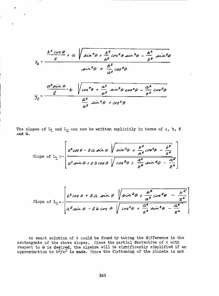
_2
b2
The slopes of L1 and L 2 can now be written explicitly in terms of a, b,and @.
Slope of _z-
V z '6z" 1b'c.._ - Za,_._-_ ,,a.,.:,_2@ ,'-b' (._,. _
0"_ zz I
---- V 7 .m
-7
An exact solution of A could be found by taking the difference in the
arctangents of the above slopes. Since the partial derivative of A with
respect to @ is desired, the algebra will be significantly simplified if an
approximation to b2/a 2 is made. Since the flattening of the planets is not
241
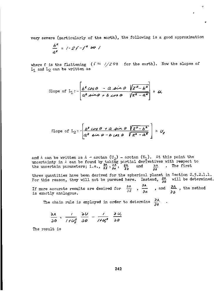
very severe (particularly of the earth), the following is a good approximation
_2-- = /-2F-., "r* _ /0.,z
where f is the flattening (_ 1/298 for the earth). Now the slopes of
L1 and L2 can be written as
- <2
Slope of Ll: Lc_2..._--_9 ¢-6 _ e
Slope of L 2:-
and A can be written as A = arctan (U2) - arctan (UI). At this point theuncertainty in A can be found bytaking partial derlvatives with respect to
_A a_ _ and _A . The firstthe uncertain parameters; i.e., _ __a ' _b _a
three quantities have been derived for the spherical planet in Section 2.5.2.1.1.
For this reason, they will not be pursued here. Instead, _AA
aA _AIf more accurate results are desired for -- , and
is exactly analogous. _Z. ' _a
The chain rule is employed in order to determine _AA .d8
will be determined.
d_A_A the method
_b
BA / bC/ / _ u,
The result is
242
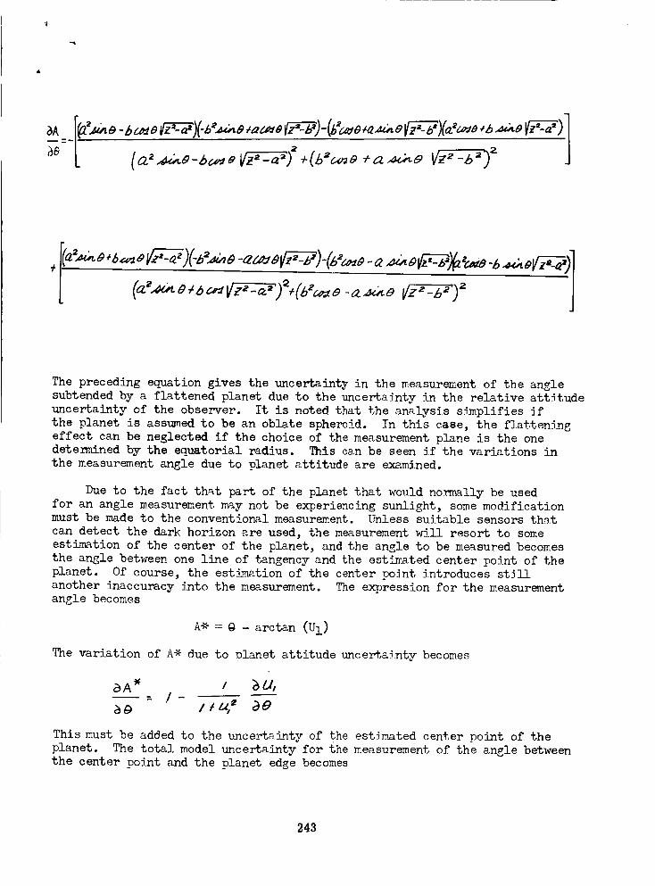
!
The preceding equation gives the uncertainty in the measurement of the angle
subtended by a flattened planet due to the uncertainty in the relative attitude
uncertainty of the observer. It is noted that the analysis s_mplifies if
the planet is assumed to be an oblate spheroid. In this case, the flatteningeffect can be neglected if the choice of the measurement plane is the one
determined by the equatorial radius. This can be seen if the variations in
the measurement angle due to planet attitude are examined.
Due to the fact that part of the planet that would no_lly be used
for an angle measurement may not be experiencing sunlight, some modificationmust be made to the conventional measurement. Unless suitable sensors that
can detect the dark horizon are used, the measurement will resort to some
estimation of the center of the planet, and the angle to be measured becomes
the angle between one line of tangency and the estimated center point of the
planet. Of course, the estimation of the center point introduces st_ll
another inaccuracy into the measurement. The expression for the measurementangle becomes
A* = @ - arctan (U1)
The variation of A* _ue to olanet attitude uncer%ainty becomes
aA _ / _U,
This must be ad@ed to the uncertainty of the estimated center point of the
planet. The total model uncertainty for the measurement of the angle between
the center point and the planet edge becomes
243
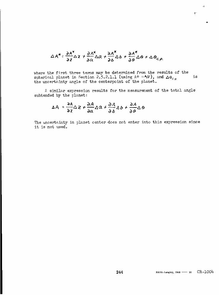
Z_A_ _A_ _A _ _A _ _A _
where the first three ter_Ls may be deten_ined from the results of the
spherical planet in Section 2.5.2.1.1 (using A*----A/E), and Z_Ocpthe uncertainty angle of the centerpoint of the planet.
is
A similar expression results for the measurement of the total angle
subtended by the planet:
_A
The uncertainty in planet center does not enter into this expression since
it is not used.
244 NASA-Langley, 1968- 30 CR-1004