Embed Size (px)
Citation preview

IIB 4F8: Image Processing and Image CodingHandout 0: Introduction
J Lasenby
Signal Processing and Communications Group,Engineering Department,
Cambridge, UK
Lent 2016
1
Introduction: 2d Image Processing
An image can take many forms and is not restricted to visualimages.Examples
1. Luminance of objects in a scene (ordinary camera)
2. Absorption characteristics of body tissue (x-ray camera)
3. Electron production of specimen scanned by electron beam(scanning electron microscope)
4. Temperature profile of a region (infra-red imaging)
5. Sidescan sonar (acoustic reflectance)
6. Seismic surveying, Earthquakes and seismic charges (often 3or even 4 dimensional)
7. Radio-telescope images
2

Some examples
Some examples of the above are shown below:
Figure 1: Scanning electron microscope image of a mosquito’s headillustrating the compound eye structure (x200)
3
Figure 2: Image of a head andshoulders taken by a 16× 16thermal (IR) imaging array
Figure 3: The 16× 16 imageinterpolated to 128× 128
4

Figure 4: False colour image ofthe cosmic microwavebackground (CMB) radiationmeasured with the Very SmallArray (VSA), Cambridge (2002)
Figure 5: Map of the CMB takenwith the WMAP telescope(2003)
5
Figure 6: Stack of scans from a seismic experiment – each trace is thereturn over time at different distances from the initial source
6

Applications
Given the importance of visual images to humans, the range ofapplications is vast. The following list is a tiny subset of possibleapplications.Astronomical imaging systems: In the past, cameras mounted onspace-craft were limited in size, weight and power consumption sothat image quality was often relatively poor - low signal to noiseratio, blurring, geometrical distortion.Computationally intensive image processing was therefore routinelyapplied to the images, and many sophisticated techniques werethereby developed. Probably the best known ‘recent’ example ofthis was the Hubble space telescope (HST) – next figure shows anexample of a picture of galaxy M87 in the early days of the HST(before optical corrections were carried out by the shuttle) beforeand after image processing and then the image after repair of thetelescope.
7
Figure 7: M87 as observed from the Hubble Space Telescope, before andafter image processing and then repaired
8

Medical applications are of great importance. One of the earliestapplications was enhancement of hairline fractures in x-ray images.Computed tomography (CT) is a technique of major importance inmedicine and is based on the Projection-Slice Theorem whichenables a 2-D image to be reconstructed from 1-D images. Theimage is reconstructed from the set of 1-D signals (projectors)taken at angles. The figure below shows the ideas behind thisprocess
Figure 8: A simulated 2d image of the head and itsradon transform – given a radon transform made upfrom 1d slices, the 2d image can be inferred.R(L) =
∫L f (x)ds(x), L line in 2D, s arclength.
Figure 9:Abdominal CTscan
9
Forensic applications. Deblurring of photographs and still images,fingerprint identification, etc. In a past case of the abduction of ateenage girl, CCT footage of the last sighting of her underwentimage processing to remove not blur, but glare which was presentin the images. The difference glare can make is illustrated in thepictures below:
Figure 10: Left hand image is with glare, right hand image is withoutglare (in these pictures glare is actually removed with a polarizer)
10

Movies and Television: flicker (interpolated frames - need motionestimation), degradations etc. The figure below gives some idea ofremoval of degradations from video footage.
Figure 11: Example ofdegraded frame from videofootage
Figure 12: Restored frame,using blotch and line removal
11
Image coding for low bandwidth environments: we wish tocompress our image data in as lossless a way as is possible in orderto transmit the data efficiently (second half of course).Computer vision – this deals with a sequence of images over time,or multiple sequences of images from which we estimate the full 3dreconstruction moving in time.
Figure 13: Three camera frames of a multiple camera setup observing amarked moving subject
Disparity Images from stereo cameras are used widely in computervision to estimate depth and perform 3D reconstruction – followingimages show left and right images and the resulting disparity map.
12

Figure 14: Left, Right and Disparity Images
[images taken from http://vision.stanford.edu/]
This is a very small sample of applications – as cheap computingbecomes increasingly available, so image processing techniques willimpinge on many more areas of everyday life, being available onmobile devices (this is already the case).
13
Image Representation and Modelling
Image processing can be broken down into a number of(overlapping) areas as shown below.
Perception Models
• visual perceptionof contrast,spatial frequenciesand colour
• image fidelitymodels
• temporal/sceneperception
Local Models
• Sampling andreconstruction
• imagequantisation
• deterministicmodels
• statistical models
Global Models
• scene analysis/AImodel
• sequential andclustering models
• imageunderstandingmodels
We will concentrate on local models but some areas (imagecoding) must take account of results obtained from perceptionmodels. One can split our local model image processing up intoseveral ‘areas’.
14

Image Enhancement
The objective of image enhancement is to accentuate particularfeatures of an image in such a way that subsequent display isimproved. The techniques do not introduce additional information.Examples are:
• Edge enhancement
• Grey level histogram equalisation
• Pseudo-colour (eg Matlab)
15
Figure 15: Original image (left) and application of adaptive histogramequalisation/contrast enhancement (right)
See http://alex.mdag.org/improc.16

Image Restoration
The objective is to restore a degraded image to its original form.An observed image can often be modelled as:
fobs(u1, u2) =∫∫
h(u1−u′1, u2−u′2)ftrue(u′1, u′2) du
′1 du
′2+n(u1, u2)
where the integral is a convolution function and h is the impulseresponse or point spread function of the imaging system and n isadditive noise. The objective of image restoration in this casewould be to estimate the original image ftrue from the observeddegraded image fobs .
17
Figure 16: Original image (left) and deconvolved image (right)
See http://www.mirametrics.com/brief maxent lab.htm.
18

Image Analysis
Image analysis is concerned with extracting features from an imagefor subsequent analysis, or processing. Reading car number plates,inspection of items on conveyor belts etc.
Figure 17: Extraction of corners from an indoor scene
19
Another example of using feature extraction for subsequentinference.
Figure 18: Dynamic surface reconstruction from grid point tracking
20

Course Contents and books
• 2d continuous Fourier transform and its properties
• Linear spatially invariant systems (LSI)
• Image digitisation and sampling – sampling schemes
• The 2d discrete Fourier transform (and mention 2d z -transform)
• Ideal image filters – the importance of phase
• Digital filter design (2d)
• Deconvolution of images
• Image enhancement
• 1. Fundamentals of digital image processing: Anil Jain (PrenticeHall) 2. Digital image processing: Gonzalez and Woods (PrenticeHall) 3. Two-dimensional signal and image processing: J S Lim(Prentice Hall)
J. Lasenby (2016)21
22

IIB 4F8: Image Processing and Image CodingHandout 1: 2D Fourier Transforms and Linear Systems
J Lasenby
Signal Processing Group,Engineering Department,
Cambridge, UK
Lent 2016
1
Course notes, Matlab programs and Example Sheet available fordownload fromwww-sigproc.eng.cam.ac.uk/ ˜jl
Now also available on the CUED Moodle site:https://www.vle.cam.ac.uk/
IB Signal and Data Analysis notes available fromwww-sigproc.eng.cam.ac.uk/ ˜jl
... and from Prof Simon Godsill’s website:www-sigproc.eng.cam.ac.uk/ ˜sjg
2

Multidimensional Signals and Systems
Will discuss 2-D signals and systems (but readily generalised tohigher dimensions). Consider the system below which has inputx(u1, u2) and output y(u1, u2)
Input image Output image
x(u1,u2) y(u1,u2)
F(.)
y(u1, u2) = F [x(u1, u2)]
Want to characterise the functional mapping F [·] between inputand output in terms of concepts such as impulse response andfrequency response. First need to generalise the concept of theFourier transform to multiple dimensions.
3
The 2d Fourier Transform
The 1-D Fourier transform G (ω) of a function g(t) is given by:
G (ω) =∫ ∞
−∞g(t) e−jωt dt
g(t) =1
2π
∫ ∞
−∞G (ω) e jωt dω
The 2-D Fourier transform of a spatial function g(u1, u2) is givenby:
G (ω1, ω2) =∫ ∞
−∞
∫ ∞
−∞g(u1, u2) e
−j(ω1u1+ω2u2) du1 du2
..with inverse 2DFT given by
g(u1, u2) =1
(2π)2
∫ ∞
−∞
∫ ∞
−∞G (ω1, ω2) e
j(ω1u1+ω2u2) dω1 dω2
4

Proving Inverse 2d Fourier Transform
Do this by direct substitution:
FT (g(u1, u2)) =
=1
(2π)2
∫ ∫ [∫ ∫G (ω′1,ω′2) e
j(ω′1u1+ω′2u2) dω′1 dω′2
]e−j(ω1u1+ω2u2) du1 du2
=1
(2π)2
∫ ∫G (ω′1,ω′2)
[∫ ∫e j((ω
′1−ω1)u1+(ω′2−ω2)u2) du1 du2
]dω′1 dω′2
=1
(2π)2
∫ ∫(2π)2G (ω′1,ω′2) δ(ω′1 −ω1)δ(ω
′2 −ω2)dω′1 dω′2
= G (ω1,ω2)
Where we have used the result that∫ ∞−∞ exp(±jωt)dω = 2πδ(t)
– see later.
5
Separability of 2d Fourier Transform
Note that the 2d Fourier transform can be rewritten as:
G (ω1, ω2) =∫ ∞
−∞e−jω1u1
∫ ∞
−∞g(u1, u2) e
−jω2u2 du2
du1
Inner integral is simply the FT of the waveform corresponding tomoving along a line in the u2-direction at some fixed position u1.This gives a function of ‘vertical’ position u1 and ‘horizontal’spatial frequency ω2. Outer integral is the Fourier transform ofthis function in the u1 direction.
6

Separability of 2d Fourier Transform – illustration
This may be illustrated by considering the 2-dimensional sinewaveg(x , y) = sin Ω1x sin Ω2y , which is shown in the figure forΩ1 = 2πf1, f1 =
116Hz and Ω2 = 2πf2, f2 =
132Hz.
7
2d sinewave example
If we first do the integration wrt y we get
F (x , ω2) = sin Ω1x
∫ ∞
−∞sin Ω2y e−jω2y dy
= jπ sin Ω1x [δ(ω2 + Ω2)− δ(ω2 −Ω2)]
8

2d sinewave example cont...
If we now do the integration in the x direction we obtain
G (ω1, ω2) = jπ [δ(ω2 + Ω2)− δ(ω2 −Ω2)]∫ ∞
−∞sin Ω1x e−jω1x dx
= −(π)2 [δ(ω1 + Ω1)− δ(ω1 −Ω1)] [δ(ω2 + Ω2)− δ(ω2 −Ω2)]
9
Illustration of spatial frequencies in images
0 50 100−1
−0.5
0
0.5
1
Figure 1: 1d sine wave
−4 −2 0 2 40
100
200
300
400
Figure 2: Spectrum of the 1dsine wave
0 50 100−1
−0.5
0
0.5
1
Figure 3: 1d sine wave – varyingfrequency
−4 −3 −2 −1 0 1 2 3 40
50
100
150
200
Figure 4: Spectrum of variablefrequency sine wave
10

20 40 60 80 100 120
20
40
60
80
100
120
Figure 5: 2d sine wave Figure 6: Spectrum of the 2dsine wave
20 40 60 80 100 120
20
40
60
80
100
120
Figure 7: 2d sine wave – varyingfrequency [spatial tilt]
Figure 8: Spectrum of variablefrequency 2d sine wave
11
20 40 60 80 100 120
20
40
60
80
100
120
Figure 9: 2d texture Figure 10: Spectrum of thetexture
20 40 60 80 100 120
20
40
60
80
100
120
Figure 11: 2d texture – varyingfrequency [spatial tilt]
Figure 12: Spectrum of variablefrequency 2d texture
12

Example of using texture to extract shape
Figure 13: Texture laid ontocylindrical pipe
Figure 14: Shape fromextraction of frequenciesfrom the texture
(Fabio Galasso, PhD Thesis, University of Cambridge 2009).
13
Properties of 2d Fourier Transforms: Spatial Shift
Consider a spatially shifted version g(u1 − µ1, u2 − µ2) of theimage g(u1, u2). The FT of the shifted image is:
G′(ω1, ω2) =
∫∫ ∞
−∞g(u1 − µ1, u2 − µ2) e
−j(ω1u1+ω2u2) du1 du2
Let u1 − µ1 = u′1 and u2 − µ2 = u
′2
G′(ω1, ω2) =
∫∫ ∞
−∞g(u
′1, u
′2) e
−j [(ω1(u′1+µ1)+ω2(u
′2+µ2)] du
′1 du
′2
= e−j(µ1ω1+µ2ω2)∫∫
g(u′1, u
′2) e
−j(ω1u′1+ω2u
′2) du
′1 du
′2
= e−j(µ1ω1+µ2ω2) G (ω1, ω2)
∴ g(u1 − µ1, u2 − µ2)⇔ e−j(µ1ω1+µ2ω2) G (ω1, ω2)
14

Properties: Frequency Shift or Spatial Modulation
Consider a spatial-frequency shifted image transformG (ω1 −Ω1, ω2 −Ω2). The FT is
G (ω1, ω2) =∫ ∞
−∞
∫ ∞
−∞g(u1, u2) e
−j(ω1u1+ω2u2) du1 du2
replace ω1 and ω2 by ω1 −Ω1 and ω2 −Ω2
G (ω1−Ω1, ω2−Ω2) =∫∫ ∞
−∞g(u1, u2) e
−j((ω1−Ω1)u1+(ω2−Ω2)u2) du1 du2
=∫∫ ∞
−∞e j(Ω1u1+Ω2u2) g(u1, u2) e
−j(ω1u1+ω2u2) du1 du2
∴ g(u1, u2)ej(Ω1u1+Ω2u2) ⇔ G (ω1 −Ω1, ω2 −Ω2)
Again, exactly as in the 1d case. In both cases, a shift in onedomain causes multiplication by an exponential in the otherdomain.
15
Useful Fourier Transforms: Impulse function
The function δ(u1, u2) is an impulse occuring at the originu1 = 0, u2 = 0 and the function δ(u1 − µ1, u2 − µ2) is an impulseoccuring at u1 = µ1, u2 = µ2.The impulse function is defined by:
limε→0
∫ ε
−ε
∫ ε
−εδ(u1, u2) du1 du2 = 1 Unit area
∫∫ ∞
−∞δ(u1−µ1, u2−µ2) f (u1, u2) du1 du2 = f (µ1, µ2) Sifting property
The Fourier transform of the 2-D impulse function is:
∆(ω1, ω2) =∫ ∞
−∞
∫ ∞
−∞δ(u1, u2) e
−j(ω1u1+ω2u2) du1 du2 = 1
∴ δ(u1, u2)⇔ 1
16
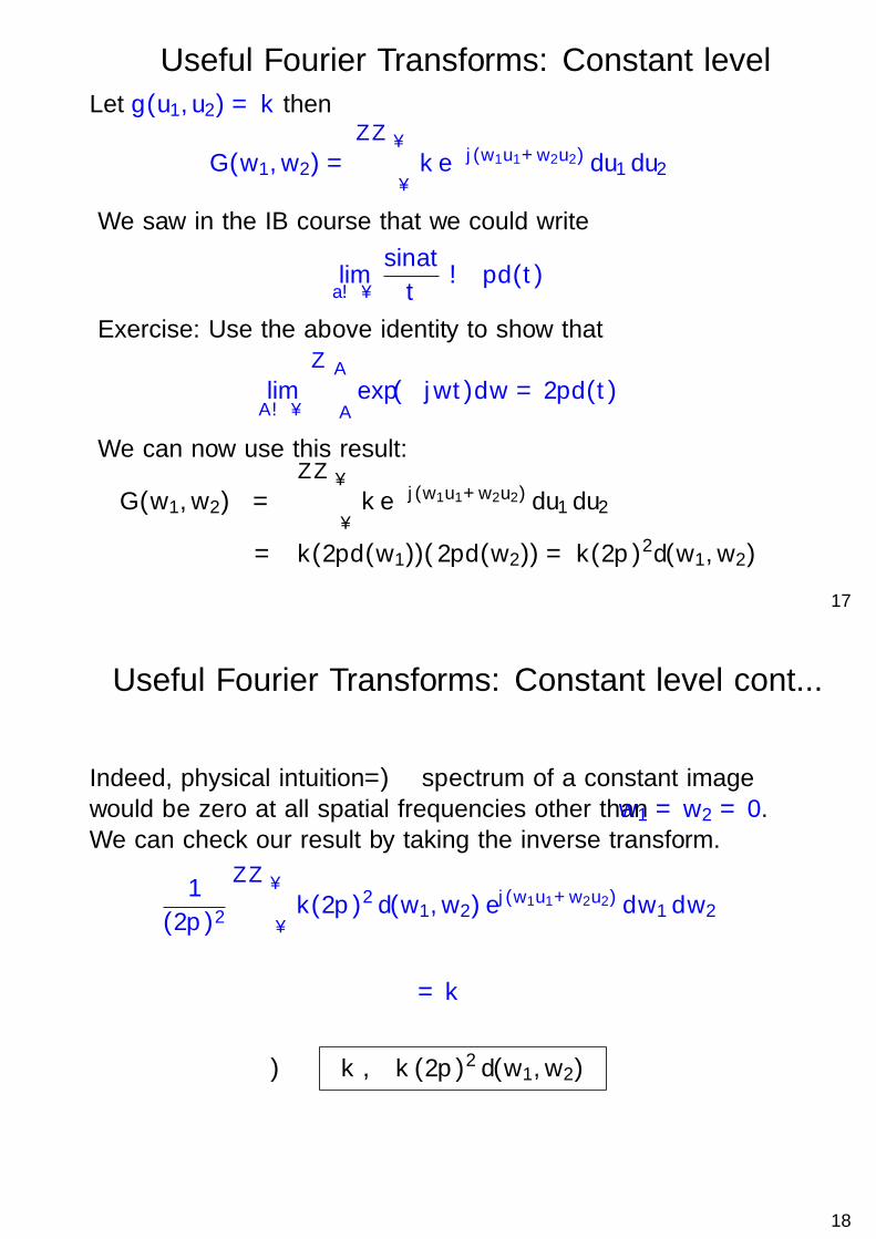
Useful Fourier Transforms: Constant level
Let g(u1, u2) = k then
G (ω1, ω2) =∫∫ ∞
−∞k e−j(ω1u1+ω2u2) du1 du2
We saw in the IB course that we could write
lima→∞
sin at
t→ πδ(t)
Exercise: Use the above identity to show that
limA→∞
∫ A
−Aexp(±jωt)dω = 2πδ(t)
We can now use this result:
G (ω1, ω2) =∫∫ ∞
−∞k e−j(ω1u1+ω2u2) du1 du2
= k(2πδ(ω1))(2πδ(ω2)) = k(2π)2δ(ω1, ω2)
17
Useful Fourier Transforms: Constant level cont...
Indeed, physical intuition =⇒ spectrum of a constant imagewould be zero at all spatial frequencies other than ω1 = ω2 = 0.We can check our result by taking the inverse transform.
1
(2π)2
∫∫ ∞
−∞k(2π)2 δ(ω1, ω2) e
j(ω1u1+ω2u2) dω1 dω2
= k
∴ k ⇔ k (2π)2 δ(ω1, ω2)
18

Useful Fourier Transforms: Complex Exponential
Let g(u1, u2) = e j(Ω1u1+Ω2u2) then
G (ω1, ω2) =∫∫ ∞
−∞e j(Ω1u1+Ω2u2) e−j(ω1u1+ω2u2) du1 du2
=∫ ∞
−∞
∫ ∞
−∞e−j [(ω1−Ω1)u1+(ω2−Ω2)u2] du1 du2
= (2π)2δ(ω1 −Ω1, ω2 −Ω2)
Note that it is also possible to see this result directly using thefrequency shift theorem:
g(u1, u2)ej(Ω1u1+Ω2u2) ⇔ G (ω1 −Ω1, ω2 −Ω2)
In this case: g(u1, u2) = 1 and G (ω1, ω2) = (2π)2δ(ω1, ω2)
∴ e j(Ω1u1+Ω2u2) ⇔ (2π)2δ(ω1 −Ω1, ω2 −Ω2)
19
Linear Systems
x(u1,u2) y(u1,u2)F(.)
y(u1, u2) = F [x(u1, u2)]
Here x(u1, u2) is the input to the linear system and y(u1, u2) isthe output. A system is linear if:
F [a x1(u1, u2) + b x2(u1, u2)] = aF [x1(u1, u2)] + bF [x2(u1, u2)]
If the input to the system is a 2-d impulse functionδ(u1 − µ1, u2 − µ2) positioned at u1 = µ1, u2 = µ2 then theresulting output image is termed the impulse responseh(u1, u2; µ1, µ2) of the system. That is:
h(u1, u2; µ1, µ2) = F [δ(u1 − µ1, u2 − µ2)]
20
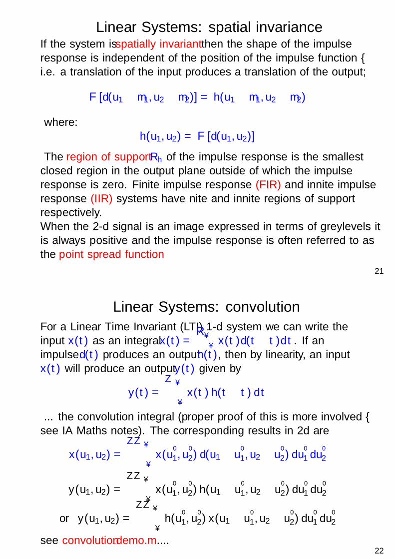
Linear Systems: spatial invarianceIf the system is spatially invariant then the shape of the impulseresponse is independent of the position of the impulse function –i.e. a translation of the input produces a translation of the output;
F [δ(u1 − µ1, u2 − µ2)] = h(u1 − µ1, u2 − µ2)
where:h(u1, u2) = F [δ(u1, u2)]
The region of support Rh of the impulse response is the smallestclosed region in the output plane outside of which the impulseresponse is zero. Finite impulse response (FIR) and infinite impulseresponse (IIR) systems have finite and infinite regions of supportrespectively.When the 2-d signal is an image expressed in terms of greylevels itis always positive and the impulse response is often referred to asthe point spread function
21
Linear Systems: convolution
For a Linear Time Invariant (LTI) 1-d system we can write theinput x(t) as an integral x(t) =
∫ ∞−∞ x(τ)δ(t − τ)dτ. If an
impulse δ(t) produces an output h(t), then by linearity, an inputx(t) will produce an output y(t) given by
y(t) =∫ ∞
−∞x(τ) h(t − τ) dτ
... the convolution integral (proper proof of this is more involved –see IA Maths notes). The corresponding results in 2d are
x(u1, u2) =∫∫ ∞
−∞x(u
′1, u
′2) δ(u1 − u
′1, u2 − u
′2) du
′1 du
′2
y(u1, u2) =∫∫ ∞
−∞x(u
′1, u
′2) h(u1 − u
′1, u2 − u
′2) du
′1 du
′2
or y(u1, u2) =∫∫ ∞
−∞h(u
′1, u
′2) x(u1 − u
′1, u2 − u
′2) du
′1 du
′2
see convolution demo.m....22
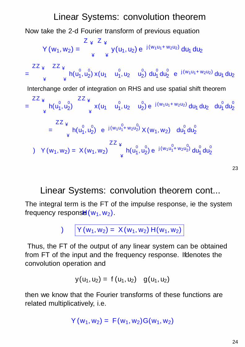
Linear Systems: convolution theorem
Now take the 2-d Fourier transform of previous equation
Y (ω1, ω2) =∫ ∞
−∞
∫ ∞
−∞y(u1, u2) e
−j(ω1u1+ω2u2) du1 du2
=∫∫ ∞
−∞
[∫∫ ∞
−∞h(u
′1, u
′2) x(u1 − u
′1, u2 − u
′2) du
′1 du
′2
]e−j(ω1u1+ω2u2) du1 du2
Interchange order of integration on RHS and use spatial shift theorem
=∫∫ ∞
−∞h(u
′1, u
′2)
[∫∫ ∞
−∞x(u1 − u
′1, u2 − u
′2) e
−j(ω1u1+ω2u2) du1 du2
]du′1 du
′2
=∫∫ ∞
−∞h(u
′1, u
′2)
[e−j(ω1u
′1+ω2u
′2) X (ω1, ω2)
]du′1 du
′2
∴ Y (ω1, ω2) = X (ω1, ω2)∫∫ ∞
−∞h(u
′1, u
′2) e
−j(ω1u′1+ω2u
′2) du
′1 du
′2
23
Linear Systems: convolution theorem cont...
The integral term is the FT of the impulse response, ie the systemfrequency response H(ω1, ω2).
∴ Y (ω1, ω2) = X (ω1, ω2)H(ω1, ω2)
Thus, the FT of the output of any linear system can be obtainedfrom FT of the input and the frequency response. If ∗ denotes theconvolution operation and
y(u1, u2) = f (u1, u2) ∗ g(u1, u2)
then we know that the Fourier transforms of these functions arerelated multiplicatively, i.e.
Y (ω1, ω2) = F (ω1, ω2)G (ω1, ω2)
24

Summary of LSI system relationships
x(u1,u2) y(u1,u2)h(u1,u2)H(ω1,ω2)X(ω1,ω2) Y(ω1,ω2)
The input-output relationships for a linear spatially-invariant (LSI)system can be summarised as:Spatial Domain
y(u1, u2) =∫∫ ∞
−∞x(u
′1, u
′2) h(u1 − u
′1, u2 − u
′2) du
′1 du
′2
=∫∫ ∞
−∞h(u
′1, u
′2) x(u1 − u
′1, u2 − u
′2) du
′1 du
′2
Frequency Domain
Y (ω1, ω2) = X (ω1, ω2)H(ω1, ω2)
25
where:
X (ω1, ω2) =∫∫ ∞
−∞x(u1, u2) e
−j(ω1u1+ω2u2) du1 du2 (Input spectrum)
x(u1, u2) =1
(2π)2
∫∫ ∞
−∞X (ω1, ω2) e
j(ω1u1+ω2u2) dω1 dω2 (Input signal)
Similarly for the output image y(u1, u2) and output spectrumY (ω1, ω2).
H(ω1, ω2) =∫∫ ∞
−∞h(u1, u2) e
−j(ω1u1+ω2u2) du1 du2 (Frequency response)
h(u1, u2) =1
(2π)2
∫∫ ∞
−∞H(ω1, ω2) e
j(ω1u1+ω2u2) dω1 dω2 (Impulse response)
J. Lasenby (2016)
26
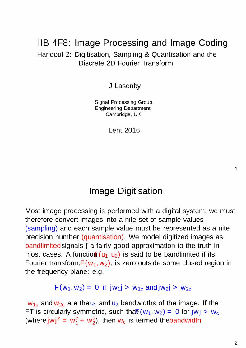
IIB 4F8: Image Processing and Image CodingHandout 2: Digitisation, Sampling & Quantisation and the
Discrete 2D Fourier Transform
J Lasenby
Signal Processing Group,Engineering Department,
Cambridge, UK
Lent 2016
1
Image Digitisation
Most image processing is performed with a digital system; we musttherefore convert images into a finite set of sample values(sampling) and each sample value must be represented as a finiteprecision number (quantisation). We model digitized images asbandlimited signals – a fairly good approximation to the truth inmost cases. A function f (u1, u2) is said to be bandlimited if itsFourier transform, F (ω1, ω2), is zero outside some closed region inthe frequency plane: e.g.
F (ω1, ω2) = 0 if |ω1| > ω1c and |ω2| > ω2c
ω1c and ω2c are the u1 and u2 bandwidths of the image. If theFT is circularly symmetric, such that F (ω1, ω2) = 0 for |ω| > ωc
(where |ω|2 = ω21 + ω2
2), then ωc is termed the bandwidth.
2

Sampling
The purpose of sampling is to convert a 2-d continuous signal intoan array of sample values from the continuous signal. There are anumber of possible different grids which can be used as the basisfor sampling: we discuss 2 of these.
Rectangular sampling
Consider the following 2-d sampling function
s(u1, u2) =∞
∑n1=−∞
∞
∑n2=−∞
δ(u1 − n1∆1, u2 − n2∆2)
which corresponds to a uniform rectangular grid of impulsefunctions spaced at intervals of ∆1 in the u1 direction and intervalsof ∆2 in the u2 direction, as shown in figure 1.
3
∆1
∆2
u2
u1
Figure 1: Rectangular sampling grid
4

Sampling on a rectangular grid
The sampled image gs(u1, u2) is given by:
gs(u1, u2) = s(u1, u2) g(u1, u2)
where g(u1, u2) is the continuous 2d function. s is periodic in u1and u2 directions, with periods ∆1 and ∆2. Can therefore write asa 2d Fourier series. Recall that a 1d periodic function f (x) (periodT ) can be written as
f (x) =∞
∑n=−∞
cnejnω0x with ω0 =2π
T
Similarly we write the 2d Fourier series for s(u1, u2) as
s(u1, u2) =∞
∑p1=−∞
∞
∑p2=−∞
c(p1, p2) ej(p1Ω1u1+p2Ω2u2) (1)
where: Ω1 =2π∆1
and Ω2 =2π∆2
5
Fourier Coefficients of s
Recall, in 1D the Fourier coefficients are given by
cn =1
T
∫ α+T
αf (x)e−jω0nxdx
We find that the 2d Fourier coefficients, c(p1, p2) are given by
c(p1, p2) =1
∆1 ∆2
∫ ∆22
− ∆22
∫ ∆12
− ∆12
s(u1, u2) e−j(p1Ω1u1+p2Ω2u2) du1 du2
Now substitute for the sampling function s(u1, u2):
c(p1, p2) =1
∆1 ∆2
∫ ∆22
− ∆22
∫ ∆12
− ∆12
[∞
∑n1=−∞
∞
∑n2=−∞
δ(u1 − n1∆1, u2 − n2∆2)
]×e−j(p1Ω1u1+p2Ω2u2) du1 du2
=⇒ c(p1, p2) =1
∆1 ∆2for all p1, p2
6

FT of sampled signal
The sampled image may then be expressed as:
gs(u1, u2) = g(u1, u2)1
∆1 ∆2
∞
∑p1=−∞
∞
∑p2=−∞
ej(p1Ω1u1+p2Ω2u2)
Using the frequency shift or spatial modulation theorem to takethe Fourier transform
g(u1, u2)ej(p1Ω1u1+p2Ω2u2) ⇔ G (ω1 −Ω1p1, ω2 −Ω2p2)
gives:
Gs(ω1, ω2) =1
∆1 ∆2
∞
∑p1=−∞
∞
∑p2=−∞
G (ω1 − p1Ω1, ω2 − p2Ω2)
It can therefore be seen that the Fourier transform or spectrum ofthe sampled 2d signal is the periodic repetition of the spectrum ofthe unsampled 2d signal (centred on the ‘grid’ points in frequencyspace) – precisely analogous to the 1d case.
7
ExampleFigures show amplitude of the spectrum of a 2d signal plotted as amesh plot and as a gray-scale plot – the spectrum here is atruncated Gaussian (therefore implying a bandlimited signal).
-0.5
0
0.5
-0.5
0
0.50
50
100
150
200
250
300
Figure 2: Spectrum of a 2Dsignal: contour
Normalised frequency
Nor
mal
ised
freq
uenc
y
-0.5 0 0.5
-0.5
-0.4
-0.3
-0.2
-0.1
0
0.1
0.2
0.3
0.4
0.5
Figure 3: Spectrum of a 2Dsignal: greyscale
8

-2-1
01
2
-2
-1
0
1
20
50
100
150
200
250
300
Figure 4: SpectrumGs(ω1, ω2) of sampled2-dimensional signal
Normalised frequency
Nor
mal
ised
freq
uenc
y
-2 -1.5 -1 -0.5 0 0.5 1 1.5 2
-2
-1.5
-1
-0.5
0
0.5
1
1.5
2
Figure 5: SpectrumGs(ω1, ω2) of sampled2-dimensional signal(greyscale)
9
Nyquist frequenciesIf the image is spatially bandlimited to ΩB1 and ΩB2 then theoriginal continuous image can be recovered from the sampledimage by ideal low-pass filtering at ΩB1, ΩB2 if the samples aretaken such that ΩB1 <
12Ω1 and ΩB2 <
12Ω2 so that the periodic
repeats of the spectrum do not overlap – this can also be writtenas:
2π
∆1> 2ΩB1
2π
∆2> 2ΩB2
2ΩB1 and 2ΩB2 are known as the 2d Nyquist frequencies. Thusthe 2d sampling theorem states that a bandlimited image sampledat or above its u1 and u2 Nyquist rates can be recovered withouterror by low-pass filtering the sampled spectrum.Sampling below the Nyquist rates causes aliasing to occur, wherewe have overlap of the repeated unsampled spectra in thefrequency plane. If aliasing occurs we are not able to recover thetrue spectrum without error.
10

Figure 6: Illustration of 2D aliasing
11
Example of Aliasing - I
12

Example of Aliasing - II
Moire
13
Example of anti-aliasing in photography
14

Recovering original signal
For sampling at or above the Nyquist frequency, we can recoverthe unsampled spectrum exactly by low-pass filtering withH(ω1, ω2) given by
H(ω1, ω2) = ∆1∆2 if ω1, ω2 ∈ R, 0 otherwise
where R is any area in the frequency plane completely containingthe spectrum of the unsampled signal – most usually we wouldtake R as [− π
∆i< ωi <
π∆i] (since π
∆i> ΩBi ).
The FT of our unsampled signal is thus
G (ω1, ω2) = H(ω1, ω2)Gs(ω1, ω2)
15
Multiplication in the spatial domain implies convolution in thefrequency domain, and vice versa; we therefore have (where h isthe inverse FT of H)
g(u1, u2) =∫ ∞
−∞
∫ ∞
−∞h(u1 − u′1, u2 − u′2)gs(u
′1, u′2)du
′1du′2
Since we can write gs as
gs(u′1, u′2) = ∑
n∑m
g(n∆1,m∆2)δ(u′1 − n∆1, u′2 −m∆2)
we can use this to write our signal g as
16
g (u1, u2) = ∑n
∑m
∫∫ ∞
−∞h(u1 − u′1, u2 − u′2)g (n∆1,m∆2)δ(u
′1 − n∆1, u
′2 −m∆2)du
′1du
′2
= ∑n
∑m
h(u1 − n∆1, u2 −m∆2)g (n∆1,m∆2)
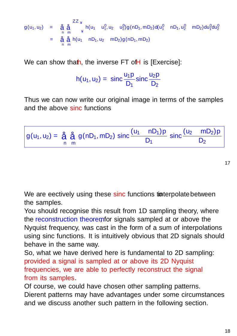
We can show that h, the inverse FT of H is [Exercise]:
h(u1, u2) = sincu1π
∆1sinc
u2π
∆2
Thus we can now write our original image in terms of the samplesand the above sinc functions
g(u1, u2) = ∑n
∑m
g(n∆1,m∆2) sinc(u1 − n∆1)π
∆1sinc
(u2 −m∆2)π
∆2
17
We are effectively using these sinc functions to interpolate betweenthe samples.You should recognise this result from 1D sampling theory, wherethe reconstruction theorem, for signals sampled at or above theNyquist frequency, was cast in the form of a sum of interpolationsusing sinc functions. It is intuitively obvious that 2D signals shouldbehave in the same way.So, what we have derived here is fundamental to 2D sampling:provided a signal is sampled at or above its 2D Nyquistfrequencies, we are able to perfectly reconstruct the signalfrom its samples.Of course, we could have chosen other sampling patterns.Different patterns may have advantages under some circumstancesand we discuss another such pattern in the following section.
18

Diamond Sampling Grid
The Diamond sampling scheme which is used in a number ofapplications is shown below:
u2
u1
∆1
∆2
Figure 7: Diamond sampling grid
19
Diamond Sampling GridRepresent the sampling grid by two separate 2d sampling functionsas illustrated below
u2
u1∆1
∆2
Figure 8: s1(u1, u2)
u2
u1
∆1
∆2
Figure 9: s2(u1, u2)
s1(u1, u2) =∞
∑n1=−∞
∞
∑n2=−∞
δ[u1 − 2 n1∆1, u2 − 2 n2∆2]
s2(u1, u2) =∞
∑n1=−∞
∞
∑n2=−∞
δ[u1 − (2 n1 + 1)∆1, u2 − (2 n2 + 1)∆2]
20

Since s1 and s2 are periodic (with periods 2∆1 and 2∆2) we canrepresent them as 2d Fourier series.
s1(u1, u2) =∞
∑p1=−∞
∞
∑p2=−∞
c1(p1, p2) ej(p1
Ω12 u1+p2
Ω22 u2)
s2(u1, u2) =∞
∑p1=−∞
∞
∑p2=−∞
c2(p1, p2) ej(p1
Ω12 u1+p2
Ω22 u2)
where Ω1 =2π
∆1and Ω2 =
2π
∆2
Thus the sampled function can be written as
gs(u1, u2) = g(u1, u2)[s1(u1, u2) + s2(u1, u2)]
=∞
∑p1=−∞
∞
∑p2=−∞
[c1(p1, p2) + c2(p1, p2)] g(u1, u2) ej(p1
Ω12 u1+p2
Ω22 u2)
21
Take the 2-D Fourier transform using the frequency shift theoremto give:
Gs(ω1, ω2) =∞
∑p1=−∞
∞
∑p2=−∞
[c1(p1, p2)+ c2(p1, p2)]G (ω1−p1Ω1
2, ω2−p2
Ω2
2)
By the usual process we can determine the Fourier coefficients
c1(p1, p2) =1
4 ∆1 ∆2
∫ ∆2
−∆2
∫ ∆1
−∆1
s1(u1, u2) e−j(p1 Ω1
2 u1+p2Ω22 u2) du1 du2
(2)
c2(p1, p2) =1
4 ∆1 ∆2
∫ ∆2
−∆2
∫ ∆1
−∆1
s2(u1, u2) e−j(p1 Ω1
2 u1+p2Ω22 u2) du1 du2
(3)
Clearly the factor 14∆1 ∆2
comes from 1T1T2
with Ti = 2∆i .
22

Substitute for s1(u1, u2) in equation 2 and interchange integral andsummation operations to give:
c1(p1, p2) =1
4 ∆1 ∆2
∞
∑n1=−∞
∞
∑n2=−∞
∫ ∆2
−∆2
∫ ∆1
−∆1
δ[u1− 2 n1∆1, u2− 2 n2∆2]
× e−j(p1Ω12 u1+p2
Ω22 u2) du1 du2
Since the only contribution to the integral will come whenn1 = n2 = 0, we have
∴ c1(p1, p2) =1
4 ∆1 ∆2
23
Similarly, substituting for s2(u1, u2) in equation 3 andinterchanging integral and summation operations gives
c2(p1, p2) =1
4∆1 ∆2
∞
∑n1=−∞
∞
∑n2=−∞
∫ 2∆2
0
∫ 2∆1
0δ[u1− (2 n1+1)∆1, u2− (2 n2+1)∆2]
× e−j(p1Ω12 u1+p2
Ω22 u2) du1 du2
note here that we change our limits to take the period between[0, 2∆1] and [0, 2∆2] (recall that we can take any interval coveringa whole period), so that the only contributions to the integral nowcome from n1 = 0 and n2 = 0 giving u1 = ∆1 and u2 = ∆2. Since(piΩi∆i )/2 = piπ we have
c2(p1, p2) =1
4 ∆1 ∆2e−j(p1+p2)π
24

Thus
c1(p1, p2) =1
4 ∆1 ∆2(4)
c2(p1, p2) =1
4 ∆1 ∆2e−j(p1+p2)π (5)
Substituting for c1(p1, p2) and c2(p1, p2) in the equation for thesampled signal spectrum gives:
Gs(ω1, ω2) =1
4 ∆1 ∆2
∞
∑p1=−∞
∞
∑p2=−∞
[1+ e−j(p1+p2)π ]G (ω1−p1Ω1
2, ω2−p2
Ω2
2)
25
Since 1 + e−j(p1+p2)π =
0, p1 + p2 = odd2, p1 + p2 = even
Gs (ω1,ω2) =1
2∆1 ∆2
∞
∑p1=−∞
∞
∑p2=−∞
G (ω1 − p1Ω1
2,ω2 − p2
Ω2
2) for p1 + p2 even
(6)
It can be seen that the spectrum of the sampled signal is theperiodic repetition of the unsampled signal spectrum, where theunsampled spectrum repeats itself at (even,even) and (odd,odd)intervals of Ω1/2 and Ω2/2 as shown in figure 10.
26

Figure 10: Spectrum of sampled signal with diamond sampling
27
Sometimes the diamond sampling grid offers an advantage overrectangular sampling as may be seen in figure 11.
Figure 11: Signal which lends itself to diamond sampling regime
Here the unsampled spectrum can be tightly enclosed by adiamond-shaped region; by sampling on a diamond grid we canthen reduce the sampling density by a factor of 2.
28

The general rule is that if an image does not contain highfrequencies simultaneously in both dimensions, then we will bebetter off sampling on a diamond grid.
For functions which are circularly symmetric or bandlimited over acircular region, it can be shown that sampling on a hexagonal gridis significantly better (requiring fewer samples) than rectangularsampling.
29
Image Quantisation
Having determined the (spatial) rate at which a 2-D signal issampled, now look at how many bits are required to represent theamplitude of each sample in a subjectively acceptable manner.
It appears that the eye is significantly less sensitive to quantisationerror in images than the sensitivity which the ear exhibits withquantised audio signals.
The generally accepted criterion for image quantisation is aresolution of 8 bits (0 to [28 − 1] = 255 or 1 to 256) whereas 16bits are required for high quality audio.
Although 8 bits gives very adequate representation for images, 10(0 to [210 − 1] = 1023 or 1 to 1024) or 12 (0 to [212 − 1] = 4095or 1 to 4096) bits are sometimes used for the very highest qualitymaterial.
30

Figures 12 to 15 show an image with successively coarserquantisation.
Quantised image 8 bits
Figure 12: Image quantisedto 8 bits: 256 grey levels (0to 255)
Quantised image 6 bits
Figure 13: Image quantisedto 6 bits: 64 grey levels (0 to63)
31
Quantised image 4 bits
Figure 14: Image quantised to4 bits: 16 grey levels (0 to 15)
Quantised image 2 bits
Figure 15: Image quantised to2 bits: 4 grey levels (0 to 3)
32
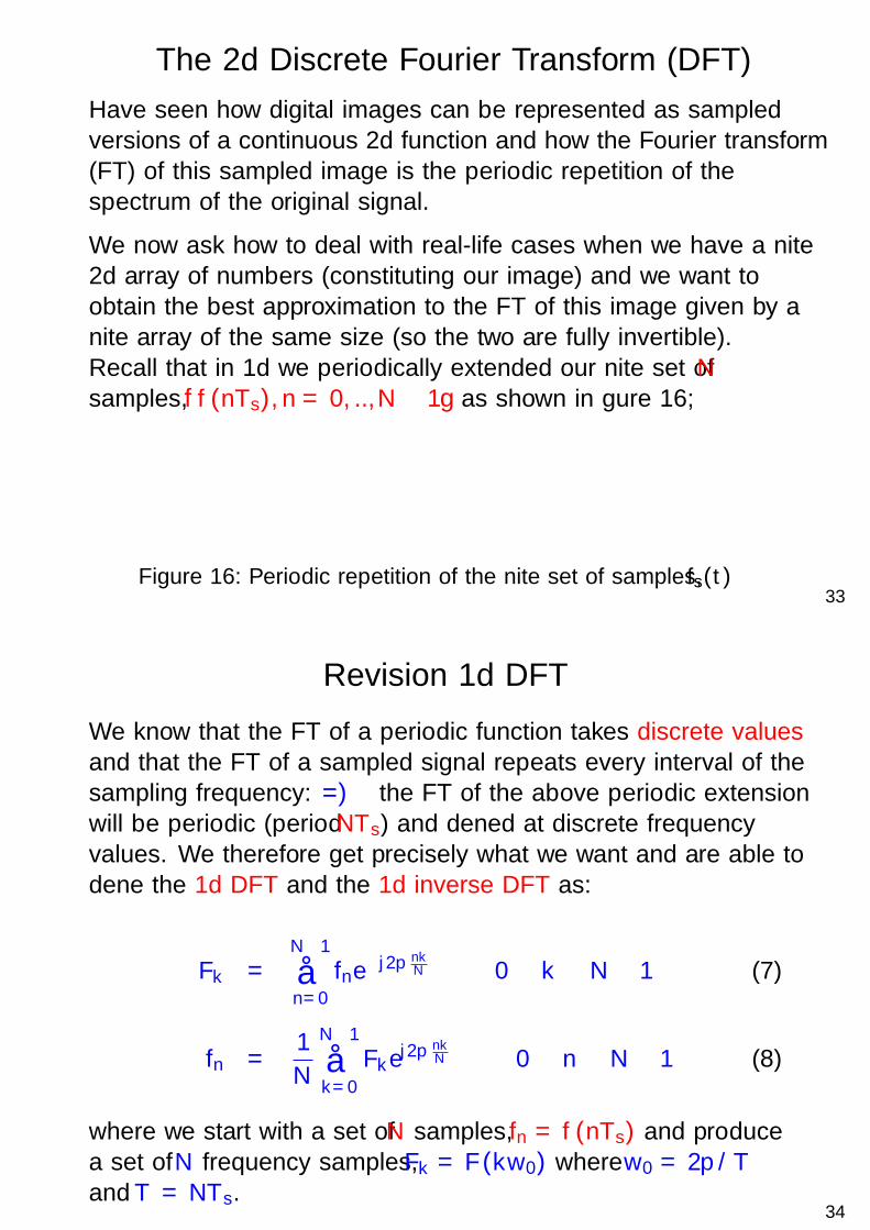
The 2d Discrete Fourier Transform (DFT)
Have seen how digital images can be represented as sampledversions of a continuous 2d function and how the Fourier transform(FT) of this sampled image is the periodic repetition of thespectrum of the original signal.
We now ask how to deal with real-life cases when we have a finite2d array of numbers (constituting our image) and we want toobtain the best approximation to the FT of this image given by afinite array of the same size (so the two are fully invertible).Recall that in 1d we periodically extended our finite set of Nsamples, f (nTs), n = 0, ..,N − 1 as shown in figure 16;
Figure 16: Periodic repetition of the finite set of samples, fs(t)33
Revision 1d DFT
We know that the FT of a periodic function takes discrete valuesand that the FT of a sampled signal repeats every interval of thesampling frequency: =⇒ the FT of the above periodic extensionwill be periodic (period NTs) and defined at discrete frequencyvalues. We therefore get precisely what we want and are able todefine the 1d DFT and the 1d inverse DFT as:
Fk =N−1∑n=0
fne−j2π nkN 0 ≤ k ≤ N − 1 (7)
fn =1
N
N−1∑k=0
Fkej2π nkN 0 ≤ n ≤ N − 1 (8)
where we start with a set of N samples, fn = f (nTs) and producea set of N frequency samples, Fk = F (kω0) where ω0 = 2π/Tand T = NTs .
34

The 2d DFT
To get the 2d DFT, again we periodically extend our image to tilethe plane as shown in figure 17:
Figure 17: Periodic repetition of the Lenna image. The solid and dottedwhite squares show two possible placings of the origin of the tiling
35
In 1d could take our period from any α to α + T ; in 2d can chooseany relevant part of the plane – Figure 17 shows the two mostcommon cases.
Solid rectangle shows the original image, dotted rectangle showsan offset section where the 1st & 3rd and the 2nd & 4th quadrantshave been interchanged. This interchange is performed by thecommand fftshift in Matlab.
36
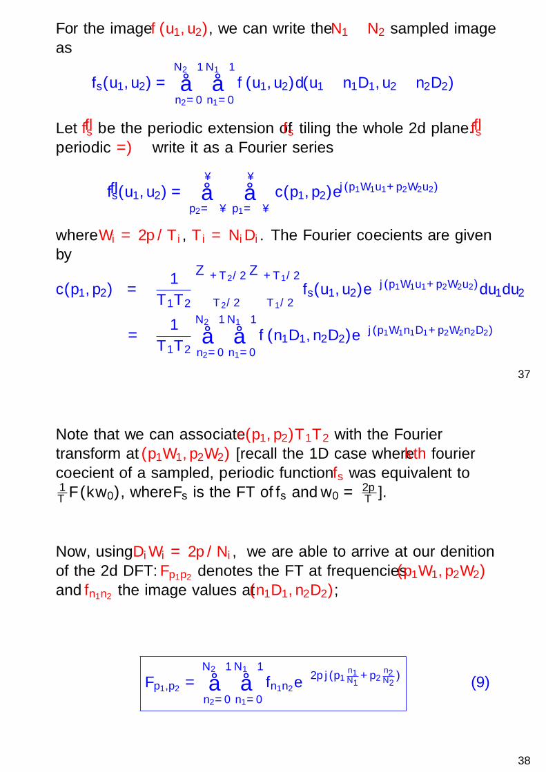
For the image f (u1, u2), we can write the N1 ×N2 sampled imageas
fs(u1, u2) =N2−1
∑n2=0
N1−1
∑n1=0
f (u1, u2)δ(u1 − n1∆1, u2 − n2∆2)
Let fs be the periodic extension of fs tiling the whole 2d plane. fsperiodic =⇒ write it as a Fourier series
fs(u1, u2) =∞
∑p2=−∞
∞
∑p1=−∞
c(p1, p2)ej(p1Ω1u1+p2Ω2u2)
where Ωi = 2π/Ti , Ti = Ni∆i . The Fourier coefficients are givenby
c(p1, p2) =1
T1T2
∫ +T2/2
−T2/2
∫ +T1/2
−T1/2fs(u1, u2)e
−j(p1Ω1u1+p2Ω2u2)du1du2
=1
T1T2
N2−1
∑n2=0
N1−1
∑n1=0
f (n1∆1, n2∆2)e−j(p1Ω1n1∆1+p2Ω2n2∆2)
37
Note that we can associate c(p1, p2)T1T2 with the Fouriertransform at (p1Ω1, p2Ω2) [recall the 1D case where kth fouriercoefficient of a sampled, periodic function fs was equivalent to1T F (kω0), where Fs is the FT of fs and ω0 =
2πT ].
Now, using ∆iΩi = 2π/Ni , we are able to arrive at our definitionof the 2d DFT: Fp1p2 denotes the FT at frequencies (p1Ω1, p2Ω2)and fn1n2 the image values at (n1∆1, n2∆2);
Fp1,p2 =N2−1
∑n2=0
N1−1
∑n1=0
fn1n2e−2πj(p1
n1N1
+p2n2N2
)(9)
38

the inverse DFT (IDFT) is similarly given by
fn1,n2 =1
N1N2
N2−1
∑p2=0
N1−1
∑p1=0
Fp1p2e2πj(n1
p1N1
+n2p2N2
)(10)
∴ we can transform an image using the 2d DFT – note that theform of this transform means that we can do it as 2 1d DFTs –giving an array of complex numbers which gives the Fouriertransform of that image.
39
2d DFT cont...
If we shift the image before transforming as shown below,
Figure 18: Original image and shifted image with 1st & 3rd and 2nd &4th quadrants interchanged
then the effect of this is to put the ‘dc level’ (pixel (1, 1)) at thecentre of the image. In most cases, it does not matter if we shiftor do not shift, but it is important to understand what effectchanging the position of the dc level has on the DFT.
40

Effects of shifting
A shift in the spatial domain implies multiplication by a complexexponential in the frequency domain. Thus if we shift our image(modulo N1 and N2) the 2D-DFT is given by
fn1+
N12 ,n2+
N22=
1
N1N2
N2−1
∑p2=0
N1−1
∑p1=0
Fp1p2e2πj([n1+
N12 ]
p1N1
+[n2+N22 ]
p2N2
)
which we can rearrange to give
fn1+
N12 ,n2+
N22=
1
N1N2
N2−1
∑p2=0
N1−1
∑p1=0
(Fp1p2eπjp1+πjp2
)e2πj(n1
p1N1
+n2p2N2
)
Thus, in the frequency domain we are applying a ±1 factor acrossthe image (since eπjpi changes from +1 to −1 moving from evento odd pixels). A one pixel shift, ie fn1,n2+1, gives an FT of
Fp1p2e2πj
p2N2 , giving a phase ramp across the image.
41
Effects of shifting – visualisation
Consider visualising our frequency data. Take a centred 2dgaussian – Both the original image and the shifted image(fftshift) have a Fourier transform which gives the DCcomponent ((0, 0) frequencies) in the top left-hand corner of theimage. If we want to visualise this so that the (0, 0) frequencycomponent is in the centre of the image then we fftshift ourtransform.
−0.5
0
0.5
−0.5
0
0.50
50
100
150
200
250
300
Figure 19: Gaussiancentred in the image
010
2030
4050
6070
0
20
40
60
800
2000
4000
6000
8000
10000
12000
14000
16000
18000
Figure 20: 2D-DFT ofgaussian
010
2030
4050
6070
0
20
40
60
800
2000
4000
6000
8000
10000
12000
14000
16000
18000
Figure 21: fftshiftapplied to 2D-DFT
42

ExerciseHere we see the same symmetric arrangement shifted to have itscentre at a different part of the image. Investigate the 2d DFTof such an image, in particular, note how the phase of the DFTdiffers between the three examples.
Figure 22: A symmetric image with the centre shifted to different parts ofthe image plane. a) centre at position (N/2 + 1,N/2 + 1) of the grid,b) centre at position (1, 1) of the grid and c) centre at position(N/2 + 2,N/2− 1) of the grid
J. Lasenby (2016)43
44

IIB 4F8: Image Processing and Image CodingHandout 3: 2D Digital Filters
J Lasenby
Signal Processing Group,Engineering Department,
Cambridge, UK
Lent 2016
1
Image FiltersIn many applications of multi-dimensional signal processing it isnecessary to apply a spatial filtering operation. In some cases 3-Dfiltering is required, operating in the 2 spatial coordinates and intime. However, at this stage, consideration will be given only to2D spatial filtering.
Figure 1: Original and filtered (convolved) versions of Lenna
2

2d Digital Filters
Have seen that we can write the output, y(u1, u2), of a linearsystem (with impulse response h(u1, u2)) and input x(u1, u2), as
y(u1, u2) =∫ ∞
−∞
∫ ∞
−∞h(u′1, u′2) x(u1 − u′1, u2 − u′2)du
′1du′2
with Y (ω1, ω2) = H(ω1, ω2)X (ω1, ω2). Call this linear system a2d digital filter and write the above in terms of discrete sums(supposing a digitised image of infinite extent):
y(n1, n2) =∞
∑p2=−∞
∞
∑p1=−∞
h(p1, p2) x (n1 − p1, n2 − p2)
3
Need to model h as discrete (again, assume infinite extent) =⇒FT is periodic. Explicity, write the discrete form of h as hs where
hs(u1, u2) =∞
∑n2=−∞
∞
∑n1=−∞
h(u1, u2)δ(u1 − n1∆1, u2 − n2∆2)
∆i is the sample spacing in the ui direction. We can then write itsFT, Hs(ω1, ω2), as∫∫ ∞
−∞
∞
∑n2=−∞
∞
∑n1=−∞
h(u1, u2)δ(u1 − n1∆1, u2 − n2∆2)e−j(ω1u1+ω2u2)du1du2
=∞
∑n2=−∞
∞
∑n1=−∞
h(n1∆1, n2∆2)e−j(ω1n1∆1+ω2n2∆2)
Note that this is just the discrete time Fourier transform (DTFT).
4

Hs(ω1, ω2) is periodic with periods Ωi = 2π/∆i ; note then thatprevious expression is the Fourier Series expansion withh(n1∆1, n2∆2) as the Fourier coefficients. Therefore
h(n1∆1, n2∆2) =1
Ω1Ω2
∫ Ω2/2
−Ω2/2
∫ Ω1/2
−Ω1/2Hs(ω1, ω2)e
j(ω1n1∆1+ω2n2∆2)dω1dω2
=∆1∆2
(2π)2
∫ π/∆2
−π/∆2
∫ π/∆1
−π/∆1
Hs(ω1, ω2)ej(ω1n1∆1+ω2n2∆2)dω1dω2
Letting ωi → (ωi∆i ), i.e. use normalised frequencies, such thatΩi → 2π
∆i∆i = 2π, we have (putting ω′i = ωi∆i and sampling intervals
of unity):
Hs(ω1, ω2) =∞
∑n2=−∞
∞
∑n1=−∞
h(n1, n2) e−j(ω1n1+ω2n2)
h(n1, n2) =1
(2π)2
∫ π
−π
∫ π
−πHs(ω1, ω2)e
j(ω1n1+ω2n2) dω1 dω2
5
2d Digital Filter relations: summary
H(ω1, ω2) =∞
∑n2=−∞
∞
∑n1=−∞
h(n1, n2) e−j(ω1n1+ω2n2)
h(n1, n2) =1
(2π)2
∫ π
−π
∫ π
−πH(ω1, ω2)e
j(ω1n1+ω2n2) dω1 dω2
(where we have dropped the subscript s on Hs). h(n1, n2) = 0outside the region of support Rh of the impulse response so that:
H(ω1, ω2) = ∑ ∑(n1,n2∈Rh)
h(n1, n2) e−j(ω1n1+ω2n2)
6

Importance of phase in images
In 1-D processing, particularly of audio signals, the phase response(essentially how the phase is altered) of any filtering operation is ofrelatively minor importance since the auditory system is insensitiveto phase.
However, perception of images is very much concerned with linesand edges.
If the filter phase response is non-linear, then the various frequencycomponents which contribute to an edge in an image will be phaseshifted with respect to each other in such a way that they nolonger add up to produce a sharp edge (i.e. dispersion takes place).
7
Original image
Figure 2: ‘Lenna’ (256× 256) pixels: original image
Take FT of above and(a) set phases to zero and take IDFT(b) set amplitudes to 1 and take IDFT
8

Image reconstructed from amplitude of spectrum Image reconstructed from phase of spectrum
Figure 3: Amplitude and Phase reconstruction
9
Zero-phase filters
If a filter frequency response is to be zero-phase then it is purelyreal so that:
H(ω1, ω2) = H∗(ω1, ω2)
Using our previous expression for H
∑ ∑(n1,n2∈Rh)
h(n1, n2) e−j(ω1n1+ω2n2) = ∑ ∑
(n1,n2∈Rh)
h∗(n1, n2) e+j(ω1n1+ω2n2)
The above equation is satisfied for all ω1 and ω2 if:
h∗(n1, n2) = h(−n1,−n2)
10
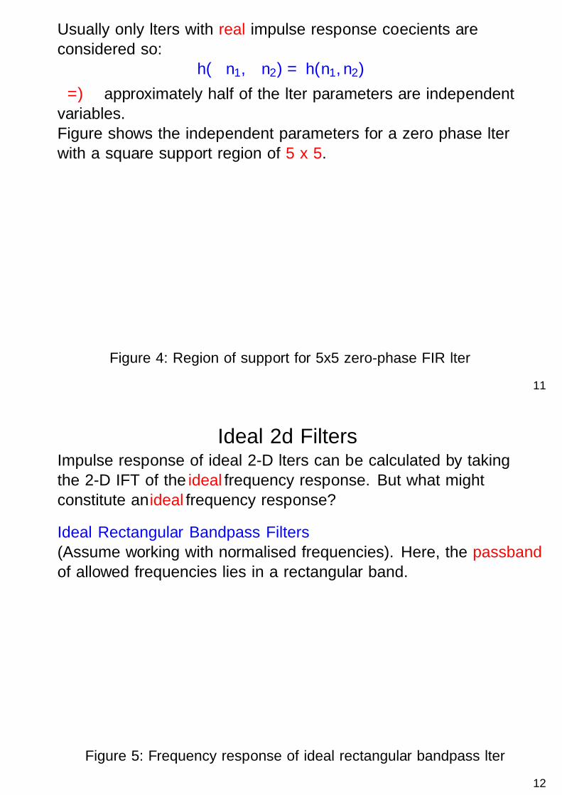
Usually only filters with real impulse response coefficients areconsidered so:
h(−n1,−n2) = h(n1, n2)
=⇒ approximately half of the filter parameters are independentvariables.Figure shows the independent parameters for a zero phase filterwith a square support region of 5 x 5.
= independent parameters h(n1,n2)
n1
n2
Figure 4: Region of support for 5x5 zero-phase FIR filter
11
Ideal 2d FiltersImpulse response of ideal 2-D filters can be calculated by takingthe 2-D IFT of the ideal frequency response. But what mightconstitute an ideal frequency response?
Ideal Rectangular Bandpass Filters(Assume working with normalised frequencies). Here, the passbandof allowed frequencies lies in a rectangular band.
AAAAAAAAAAAAAAAAAAAAAAAAAAAAAAAAAAAAAAAAAAAAAAAAAAAAAAAAAAAAAAAAAAAAAAAAAAAAAAAAA
π
− π π
− π
ΩU1
ΩU2
ΩL1
ΩL2
ω1
ω2
Figure 5: Frequency response of ideal rectangular bandpass filter
12
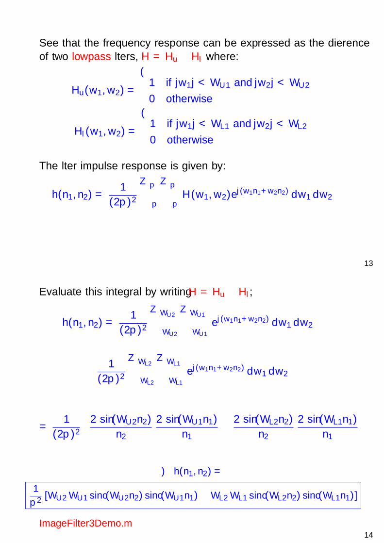
See that the frequency response can be expressed as the differenceof two lowpass filters, H = Hu −Hl where:
Hu(ω1, ω2) =
1 if |ω1| < ΩU1 and |ω2| < ΩU2
0 otherwise
Hl (ω1, ω2) =
1 if |ω1| < ΩL1 and |ω2| < ΩL2
0 otherwise
The filter impulse response is given by:
h(n1, n2) =1
(2π)2
∫ π
−π
∫ π
−πH(ω1, ω2)e
j(ω1n1+ω2n2) dω1 dω2
13
Evaluate this integral by writing H = Hu −Hl ;
h(n1, n2) =1
(2π)2
∫ ΩU2
−ΩU2
∫ ΩU1
−ΩU1
e j(ω1n1+ω2n2) dω1 dω2−
1
(2π)2
∫ ΩL2
−ΩL2
∫ ΩL1
−ΩL1
e j(ω1n1+ω2n2) dω1 dω2
=1
(2π)2
[2 sin(ΩU2n2)
n2
2 sin(ΩU1n1)
n1− 2 sin(ΩL2n2)
n2
2 sin(ΩL1n1)
n1
]
∴ h(n1, n2) =
1
π2[ΩU2 ΩU1 sinc(ΩU2n2) sinc(ΩU1n1)−ΩL2 ΩL1 sinc(ΩL2n2) sinc(ΩL1n1)]
ImageFilter3Demo.m14

Note: if we do not work with normalised frequencies but insteadtake into account the sampling intervals, ∆1 and ∆2 (where weassume that ΩU1 and ΩU2 are less than π/∆1 and π/∆2
respectively, the previous expression is written as
h(n1∆1, n2∆2) =∆1∆2
π2[ΩU2 ΩU1 sinc(ΩU2n2∆2) sinc(ΩU1n1∆1)
−ΩL2 ΩL1 sinc(ΩL2n2∆2) sinc(ΩL1n1∆1)]
15
Alternative ideal rectangular bandpass filter
π
− π π
− π
AAAAAAAAAAAAAAAAAAAAAAAAA
AAAAAAAAAAAAAAAAAAAAAAAAA
AAAAAAAAAAAAAAAAAAAAAAAAA
AAAAAAAAAAAAAAAAAAAAAAAAA
ΩU1
ΩU2
ΩL1
ΩL2
ω1
ω2
Figure 6: Frequency response of ideal separable rectangular bandpass filter
16
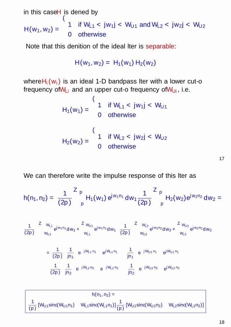
in this case H is defined by
H(ω1, ω2) =
1 if ΩL1 < |ω1| < ΩU1 and ΩL2 < |ω2| < ΩU2
0 otherwise
Note that this definition of the ideal filter is separable:
H(ω1, ω2) = H1(ω1)H2(ω2)
where Hi (ωi ) is an ideal 1-D bandpass filter with a lower cut-offfrequency of ΩLi and an upper cut-off frequency of ΩUi , i.e.
H1(ω1) =
1 if ΩL1 < |ω1| < ΩU1
0 otherwise
H2(ω2) =
1 if ΩL2 < |ω2| < ΩU2
0 otherwise
17
We can therefore write the impulse response of this filter as
h(n1, n2) =1
(2π)
∫ π
−πH1(ω1) e
jω1n1 dω11
(2π)
∫ π
−πH2(ω2)e
jω2n2 dω2 =
1
(2π)
[∫ −ΩL1
−ΩU1
e jω1n1dω1 +∫ ΩU1
ΩL1
e jω1n1dω1
]1
(2π)
[∫ −ΩL2
−ΩU2
e jω2n2dω2 +∫ ΩU2
ΩL2
e jω2n2dω2
]
=1
(2π)
[1
jn1
(e−jΩL1 n1 − e jΩL1 n1
)− 1
jn1
(e−jΩU1 n1 − e jΩU1 n1
)]
× 1
(2π)
[1
jn2
(e−jΩL2 n2 − e−jΩL2 n2
)− 1
jn2
(e−jΩU2 n2 − e jΩU2 n2
)]
h(n1, n2) =
1
(π)[ΩU1sinc(ΩU1n1)−ΩL1sinc(ΩL1n1)]
1
(π)[ΩU2sinc(ΩU2n2)−ΩL2sinc(ΩL2n2)]
18

Ideal circularly symmetric bandpass filter
In some cases preferential treatment should not be given tofrequency components in any particular direction, =⇒ circularlysymmetric frequency responses required:In this case our frequency response is given by
H(ω1, ω2) =
1 if ΩL < | ω| < ΩU
0 otherwise
where ω2 = ω21 + ω2
2.π
− π
π− π
AAAAAAAAAAAAAAAAAAAAAAAAAAAAAAAAAAAAAAAAAAAAAAAAAAAAAAAAAAAAAAAAAAAAAAAAAAAAAAAAA
ΩUΩL
ω1
ω2
Figure 7: Frequency response of ideal circular bandpass filter19
The filter impulse response is then given by:
h(n1, n2) =1
(2π)2
∫ π
−π
∫ π
−πH(ω1, ω2)e
j(ω1n1+ω2n2) dω1 dω2
Transform to polar coordinates r , θ as follows:
ω1 = r cos(θ) and ω2 = r sin(θ)
r2 = ω21 + ω2
2 , tan(θ) =ω2
ω1and elemental area=r dr dθ
The exponent in the complex exponential of the integrand may bewritten as:
j(ω1 n1+ω2 n2) = j r [n1 cos(θ)+n2 sin(θ)] = j r√(n21+n22) sin(θ +φ)
where: tan(φ) = n1n2
20

The impulse response may then be written as:
h(n1, n2) =1
(2π)2
∫ ΩU
ΩL
∫ π
−πe j r√(n21+n22) sin(θ+φ) r dθ dr =
1
(2π)2
∫ ΩU
ΩL
r∫ π
−πcos [rβ sin(θ + φ)] + j sin [rβ sin(θ + φ)] dθdr
where β =√(n21 + n22). A little thought shows that the periodic
property of sin(θ) ensures that the imaginary part of the expressionfor h(n1, n2) is zero. Thus we must now evaluate the followingintegral:
1
(2π)2
∫ ΩU
ΩL
r∫ π
−π
cos[r√(n21 + n22) sin(θ + φ)
]dθ dr
21
Substitute θ′ = θ + φ.
1
(2π)2
∫ ΩU
ΩL
r∫ φ+π
φ−π
cos[r√(n21 + n22) sin(θ′)
]dθ′ dr
θ′integrand is clearly a periodic function with period 2π, and sincewe know that for any function f (t) such that f (t) = f (t + nT ),we have ∫ T
0f (t)dt =
∫ α+T
αf (t)dt
we can rewrite our integral as
1
(2π)2
∫ ΩU
ΩL
r∫ π
−π
cos[r√(n21 + n22) sin(θ)
]dθ dr
= 21
(2π)2
∫ ΩU
ΩL
r∫ π
0
cos[r√(n21 + n22) sin(θ)
]dθ dr
22

h(n1, n2) can now be directly written in terms of the 0th orderBessel function, J0 where J0(x) =
1π
∫ π0 cosx sin(θ) dθ
h(n1, n2) =1
(2π)
∫ ΩU
ΩL
r J0[r√(n21 + n22)] dr
Let r√(n21 + n22) = x then:
h(n1, n2) =1
2π(n21 + n22)
∫ ΩU√(n21+n22)
ΩL√(n21+n22)
x J0(x) dx
Now if J1(.) is the 1st order Bessel function of the first kind where∫x J0(x) dx = x J1(x) =⇒
h(n1, n2) =1
2π√(n21 + n22)
ΩUJ1[
√(n21 + n22)ΩU ]−ΩLJ1[
√(n21 + n22)ΩL]
Thus, the IR is the difference of two first order Bessel functions.There are many examples of the use of this, one such use is inastronomy. 23
Impulse response for circularly symmetric bandpass filter
Figure 8: Inverse FT for four cases of circularly symmetric bandpass filters
J. Lasenby (2016)24

IIB 4F8: Image Processing and Image CodingHandout 4: 2D Digital Filter Design
J Lasenby
Signal Processing Group,Engineering Department,
Cambridge, UK
Lent 2016
1
2-D Digital Filter Design
In designing and using digital filters we firstly specify thecharacteristics of the filter, secondly we design the filter and thirdlywe implement the filter in a discrete setting.
Here we suppose that we are dealing only with real data and thatwe therefore require a real impulse response, h(n1, n2) so that theprocessed image is also real. We will also demand that the impulseresponse is bounded, implying stability, i.e.
∞
∑n1=−∞
∞
∑n2=−∞
|h(n1, n2)| < ∞
An unbounded output will cause many difficulties in practice,possible system overload being one of them.
2

Have seen that the impulse responses of linear systems can beeither finite or infinite =⇒ finite impulse response (FIR) orinfinite impulse response (IIR) filters. Since we require theboundedness condition, we will restrict our attention to FIR filters.Have also seen that a zero-phase 2d filter(H(ω1, ω2) = H∗(ω1, ω2)) does not disturb the phasecharacteristics of the image; important for visual perception. =⇒limit our discussion to zero-phase FIR filters with real impulseresponse.In general a filter obtained by inverse Fourier transforming somedesired zero-phase 2-D frequency response will not have a finitesupport. However a number of different techniques are availablefor the design of 2-D digital filters in which the support is finite.We will just look at one technique here, the windowing method(another common technique is the frequency transformationmethod – discussions of this can be found in the listed textbooks).
3
Figure 1: Frequency responses of circularly symmetric ideal filters:lowpass, highpass, bandpass and bandstop
Ideal circularly symmetric filters are shown in figure 1. Ideally,these regions are well delineated, i.e. a lowpass filter only haspassband and stopband regions.
4

The Window Method
Assume that the desired frequency response Hd (ω1, ω2) is given –have seen that the desired impulse response hd (n1, n2) can beobtained by taking the inverse FT of Hd .
Idea of the window design method is to multiply the infinitesupport filter by a window function w(n1, n2) which forces theimpulse response coefficients h(n1, n2) to zero for n1, n2 6∈ Rh
where Rh is the desired support region.
hd (n1, n2) =1
(2π)2
∫ π
−π
∫ π
−πHd (ω1, ω2)e
j(ω1n1+ω2n2) dω1 dω2
The filter with finite support is given by:
h(n1, n2) = hd (n1, n2)w(n1, n2)
5
Have seen that if hd (n1, n2) and w(n1, n2) satisfy the zero-phaserequirement, i.e.
hd (−n1,−n2) = hd (n1, n2) and w(−n1,−n2) = w(n1, n2)
then the resulting filter will be zero-phase, since the above implythat h(−n1,−n2) = h(n1, n2).The frequency response H(ω1, ω2) of the resulting filter can beexpressed in terms of the desired frequency response Hd (ω1, ω2)and the Fourier transform W (ω1, ω2) of the window functionw(n1, n2) as follows.
H(ω1, ω2) = ∑ ∑(n1,n2∈Rh)
h(n1, n2) e−j(ω1n1+ω2n2)
=∞
∑n2=−∞
∞
∑n1=−∞
w(n1, n2) hd (n1, n2) e−j(ω1n1+ω2n2)
6

Substituting for hd (n1, n2) gives:
H(ω1,ω2) =
∞
∑n1,n2=−∞
w (n1, n2)
[1
(2π)2
∫∫ π
−πHd (Ω1,Ω2)e
j(Ω1n1+Ω2n2)dΩ1dΩ2
]e−j(ω1n1+ω2n2)
=1
(2π)2
∫∫ π
−πHd (Ω1,Ω2)
∞
∑n1,n2=−∞
w (n1, n2)ej [(ω1−Ω1)n1+(ω2−Ω2)n2 ]dΩ1dΩ2
But the summation term is simply the 2-D FT of the windowfunction evaluated at frequencies ω1 −Ω1, ω2 −Ω2.
∴
H(ω1,ω2) =1
(2π)2
∫∫ π
−πHd (Ω1,Ω2)W ((ω1 −Ω1), (ω2 −Ω2)) dΩ1 dΩ2
W (ω1,ω2) =∞
∑n2=−∞
∞
∑n1=−∞
w (n1, n2) e−j(ω1n1+ω2n2)
7
Thus the actual filter frequency response H(ω1, ω2) is given bythe convolution of the desired frequency response Hd (ω1, ω2)with the window function spectrum W (ω1, ω2).
This is exactly as we should expect since we multiply in the spatialdomain and must therefore convolve in the frequency domain.
Thus the effect of the window is to smooth Hd – clearly we wouldprefer to have the mainlobe width of W (ω1, ω2) small so that Hd
is changed as little as possible. We also want sidebands of smallamplitude so that the ripples in the (ω1, ω2) plane outside theregion of interest are kept small.
Next – look at methods of producing window functions.
8

Product of 1-D Windows
One popular method for obtaining a 2-D window is to simply takethe product of two 1-D windows:
w(n1, n2) = w1(n1) w2(n2)
If the above holds, it is not hard to see that the FT of W is alsoseparable, i.e.
W (ω1, ω2) = W1(ω1) W2(ω2)
Note also that if the desired frequency response Hd (ω1, ω2) isseparable then the desired impulse response hd (n1, n2) is alsoseparable (clear from previous equations).Thus the windowed impulse response is also separable and thewhole design process may reduce essentially to that of designingtwo 1-D filters. 9
Rectangular Window
We now investigate the spectra of a number of window functionsformed from the product of 1-D windows.
First consider a rectangular window function given simply by
w(u1, u2) =
1 if |u1| < U1 and |u2| < U2
0 otherwise
or, since w is separable we have w = w1w2 where
wi (ui ) =
1 if |ui | < Ui
0 otherwise
10

-0.5
0
0.5
-0.5
0
0.50
50
100
150
200
250
Spectrum of product of rectangular windows, N= 15*15
Figure 2: Spectrum of product of rectangular windows, support = 15×15
Figure 2 is formed by taking the inverse FT of a zero-paddedversion of the array/image w(n1, n2).
11
Cosine WindowConsider a 1-d cosine function window,
w(u1) =
cos(π u1
U1) if |u1| < U1
0 otherwise
Taking the FT of this can be shown to give
W1(ω1) = U1sinc(π −ω1U1) + sinc(π + ω1U1)
Figure 3: Spectrum of a 1d cosine window
This is hardly ideal!12

Hamming Window
The 1d Hamming window function is simply
w(u1) =
0.54 + 0.46 cos(π u1
U1) if |u1| < U1
0 otherwise
Note, that when u1 = 0, w = 1, when u1 = U1/2, w = 0.54 andwhen u1 = U1, w = 0.54− 0.46 = 0.08. Thus the 1d Hammingwindow decays relatively slowly down to a value of 0.08 atu1 = U1. The 2d Hamming window is therefore defined as
w (u1, u2) =
[0.54+ 0.46 cos(π u1
U1)] [
0.54+ 0.46 cos(π u2U2
)]
if |u1| < U1 |u2| < U2
0 otherwise
13
-0.5
0
0.5
-0.5
0
0.50
10
20
30
40
50
60
Spectrum of product of Hamming windows, N= 15*15
Figure 4: Spectrum of product of Hamming windows,support = 15×15
Again, Figure 4 is formed by taking the FT of a zero-paddedversion of array/image w(n1, n2) given on previous slide.
14

Kaiser Window
The 1d Kaiser window function is given by
w(u1) =
Io (β√(1−( u1
U1)2)
Io (β)if |u1| < U1
0 otherwise
Here I0(.) is the modified Bessel function of the 1st kind of orderzero. The parameter β allows the spectral mainlobe performanceto be traded against spectral sidelobe performance.
Increasing β widens the mainlobe and increases the attenuation ofthe sidelobes.
15
-0.5
0
0.5
-0.5
0
0.50
20
40
60
80
100
Spectrum of product of Kaiser windows, N= 15*15
Figure 5: Spectrum of product of Kaiser windows, β = 3, support =15×15
We see that the rectangular window has a good mainlobe behaviour(small width) but a poor sidelobe behaviour (large peaks); the Hammingwindow has a moderate mainlobe behaviour but fairly good sidelobebehaviour; for the Kaiser window the relative behaviour of the main andside-lobes can be controlled by the parameter β.
16

Windowing ideal circularly symmetric filters
Now consider ideal circularly symmetric lowpass filters – use thebandpass filters we have derived previously with ΩL = 0. We haveseen that the desired impulse response, hd (n1, n2) of such a filteris given by
h(n1, n2) =1
2π√(n21 + n22)
ΩU J1[
√(n21 + n22)ΩU ]
We now apply the separable 2d window functions to this impulseresponse – again, use rectangular, Hamming and Kaiser. To findthe new impulse response, we multiply by the window and to findthe new frequency response we convolve Hd with the FT of thewindow.
17
Rectangular window
The impulse and frequency responses of an ideal circular low-passfilter, with a normalised cut-off frequency of Ω = 0.25, designedusing a rectangular window are shown below
0
5
10
15
0
5
10
15-0.05
0
0.05
0.1
0.15
0.2
Rectangular windows, N= 15*15
Figure 6: LP filter impulseresponse, rectangular windowproduct, support = 15×15
-0.5
0
0.5
-0.5
0
0.50
0.2
0.4
0.6
0.8
1
1.2
Rectangular windows, N= 15*15
Figure 7: LP filter frequencyresponse, rectangular windowproduct, support = 15×15
18

Hamming window
The impulse and frequency responses of an ideal circular low-passfilter, with a normalised cut-off frequency of Ω = 0.25, designedusing a Hamming window are shown below
0
5
10
15
0
5
10
15-0.05
0
0.05
0.1
0.15
0.2
Hamming windows, N= 15*15
Figure 8: LP filter impulseresponse, Hamming windowproduct, support = 15×15
-0.5
0
0.5
-0.5
0
0.50
0.2
0.4
0.6
0.8
1
1.2
Hamming windows, N= 15*15
Figure 9: LP filter frequencyresponse, Hamming windowproduct, support = 15×15
19
Kaiser window
The impulse and frequency responses of an ideal circular low-passfilter, with a normalised cut-off frequency of Ω = 0.25, designedusing a Kaiser window are shown below
0
5
10
15
0
5
10
15-0.05
0
0.05
0.1
0.15
0.2
Kaiser windows, N= 15*15
Figure 10: LP filter impulseresponse, Kaiser window(β = 3), support = 15×15
-0.5
0
0.5
-0.5
0
0.50
0.2
0.4
0.6
0.8
1
1.2
Kaiser windows, N= 15*15
Figure 11: LP filter frequencyresponse, Kaiser (β = 3)window, support = 15×15
20

Rotation of 1-D Windows
A second approach to implementing the window design method isto obtain a 2-D continuous window function w(u1, u2) by rotatinga 1-D continuous window w1(u).
w(u1, u2) = w1(u)|u=√(u21+u22)
The continuous 2-D window is then sampled to produce a discrete2-D window w(n1, n2):
w(n1, n2) = w(u1, u2)|u1=n1 ∆1, u2=n2 ∆2
The spectrum Ws(ω1, ω2) of the 2-D discrete window is given by:(see derivation of 2-D sampling theorem)
21
Ws(ω1, ω2) =1
∆1∆2
∞
∑p2=−∞
∞
∑p1=−∞
W (ω1 − p1Ω1, ω2 − p2Ω2)
where:
Ω1 =2π
∆1, Ω2 =
2π
∆2
and W (ω1, ω2) is the Fourier transform of the continuous 2-Dwindow w(u1, u2). Note that W is in general not equivalent to therotated form of the 1d FT.
Note that even if W (ω1, ω2) has circular symmetry the resultingWs(ω1, ω2) will not necessarily be symmetric as a result ofpossible aliasing.
Following figures show the spectra of a number of windowfunctions formed by rotating 1-D window functions.
22

Spectrum of rotated rectangular window
-0.5
0
0.5
-0.5
0
0.50
50
100
150
Spectrum of rotated rectangular window, N= 15*15
Figure 12: Spectrum of rotated rectangular window, support = 15×15
23
Spectrum of rotated Hamming window
-0.5
0
0.5
-0.5
0
0.50
10
20
30
40
50
60
Spectrum of rotated Hamming window, N= 15*15
Figure 13: Spectrum of rotated Hamming window, support = 15×15
24

Spectrum of rotated Kaiser window
-0.5
0
0.5
-0.5
0
0.50
20
40
60
80
100
Spectrum rotated Kaiser window, N= 15*15
Figure 14: Spectrum of rotated Kaiser window (β = 3), support = 15×15
25
Impulse and Frequency response of windowed circular LPfilters
As we did with the separable windows, we can now look at theimpulse and frequency responses of circular low-pass filters, with anormalised cut-off frequency of Ω = 0.25, designed using thevarious rotated windows.
Once again to obtain the impulse response we simply multiply theideal impulse response with the window and to obtain thefrequency response, we convolve the ideal frequency response withthe FT of the window. The derived frequency responses for thethree types of windowing functions we are considering here areshown in the following figures.
26

h and H of a windowed LP filter – rectangular window
0
5
10
15
0
5
10
15-0.05
0
0.05
0.1
0.15
0.2
Rotated rectangular window, N= 15*15
Figure 15: LP filter impulseresponse, rotated rectangularwindow, support = 15×15
-0.5
0
0.5
-0.5
0
0.50
0.2
0.4
0.6
0.8
1
1.2
Rotated rectangular window, N= 15*15
Figure 16: LP filter frequencyresponse, rotated rectangularwindow, support = 15×15
27
h and H of a windowed LP filter – Hamming window
0
5
10
15
0
5
10
15-0.05
0
0.05
0.1
0.15
0.2
Rotated Hamming window, N= 15*15
Figure 17: LP filter impulseresponse, rotated Hammingwindow, support = 15×15
-0.5
0
0.5
-0.5
0
0.50
0.2
0.4
0.6
0.8
1
Rotated Hamming window, N= 15*15
Figure 18: LP filter frequencyresponse, rotated Hammingwindow, support = 15×15
28

h and H of a windowed LP filter – Kaiser window
0
5
10
15
0
5
10
15-0.05
0
0.05
0.1
0.15
0.2
Rotated Kaiser window, N= 15*15
Figure 19: LP filter impulseresponse, rotated Kaiserwindow, support = 15×15
-0.5
0
0.5
-0.5
0
0.50
0.2
0.4
0.6
0.8
1
Rotated Kaiser window, N= 15*15
Figure 20: LP filter frequencyresponse, rotated Kaiserwindow, support = 15×15
J. Lasenby (2016)29
30
IIB 4F8: Image Processing and Image CodingHandout 5 : Image Deconvolution
J Lasenby
Signal Processing Group,Engineering Department,
Cambridge, UK
Lent 2016
1
Introduction to Deconvolution
We are often concerned with estimating an image x from data ymeasured with an imperfect instrumentation system. Typically,blurring is introduced as a result of an imperfect optical systemand noise d as a result of an imperfect imaging device.The observed image y(u1, u2) may be expressed as:
y(u1, u2) = f [x(u1, u2)] + d(u1, u2)
where f (.) is, in general, a nonlinear function of the original imagex(u1, u2). However we first consider only the case of lineardistortion.
y(u1, u2) = L [x(u1, u2)] + d(u1, u2)
where the linear operator is a 2-dimensional convolution:2

L [x(u1, u2)] =∫ ∫
h(v1, v2)x(u1 − v1, u2 − v2)dv1dv2
where h is the impulse response or point spread function.Assume a discrete space model:
y(n1, n2) = L [x(n1, n2)] + d(n1, n2)
where:
L [x(n1, n2)] =∞
∑m2=−∞
∞
∑m1=−∞
h(m1,m2)x(n1 −m1, n2 −m2)
Consider first the case where there is no noise and the objective isto recover the image x(n1, n2) from the observations. Assume thatthe impulse response of the distorting system is known.
3
Deconvolution of Noiseless Images
Problem: given observations y(n1, n2) and knowledge of thefunction h(m1,m2) obtain an estimate of the original imagex(u1, u2) where:
y(n1, n2) = ∑m1
∑m2
h(m1,m2)x(n1 −m1, n2 −m2)
x and y are convolved =⇒ take the Fourier transform of eachside of the above to give:
Y (ω1, ω2) = H(ω1, ω2)X (ω1, ω2)
where: H(ω1, ω2) = ∑∞n2=−∞ ∑∞
n1=−∞ h(n1, n2)e−j(ω1n1+ω2n2)
∴ X (ω1, ω2) =Y (ω1, ω2)
H(ω1, ω2)
=⇒ x(n1, n2) =1
(2π)2
∫ π
−π
∫ π
−πX (ω1, ω2)e
j(ω1n1+ω2n2)dω1dω2
4

Note: If H(ω1, ω2) has zeros, then the inverse filter, 1/H, willhave infinite gain. i.e. if 1/H is very large (or indeed infinite),small noise in the regions of the frequency plane where these largevalues of 1/H occur can be hugely amplified. To counter this wecan threshold the frequency response, leading to the so-called,pseudo-inverse or generalised inverse filter Hg (ω1, ω2) given by
Hg (ω1, ω2) =
1
H(ω1,ω2)1
|H(ω1,ω2| < γ
0 otherwise(1)
or
Hg (ω1, ω2) =
1
H(ω1,ω2)1
|H(ω1,ω2| < γ
γ |H(ω1,ω2|H(ω1,ω2)
otherwise(2)
Clearly for 1|H(ω1,ω2| ≥ γ in equation 2, the modulus of the filter is
set as γ, whereas in previous equation it is set as 0.
5
Although the pseudo-inverse filter may perform reasonably well onnoiseless images, the performance is unsatisfactory with evenmildly noisy images due to the still significant noise gain atfrequencies where H(ω1, ω2) is relatively small; =⇒ investigatethe possibility of taking the additive noise into account in a moreformal manner.
Now look at two examples of inverse filtering.
First use the inverse filtering method on an image which has beenconvolved with a gaussian (assuming knowledge of the blurringgaussian).
Then use the same inverse filtering operation when the originalimage has been convolved with the same gaussian and thensubjected to additive noise.
6

Results of Inverse Filterng
zero padded original image
Figure 1: 192× 192 original image;central 128× 128 of Lenna paddedwith zeros
blurred image
Figure 2: Previous image blurredwith a gaussian
7
Results of Inverse Filtering
Figure 3: Inverse filter applied tonoiseless blurred image
Figure 4: Inverse filter applied toblurred image plus noise (0.01)
8

Results of Inverse Filtering
Figure 5: Inverse filter applied toblurred image plus noise (0.1)
Figure 6: Inverse filter applied toblurred image plus noise (0.5)
9
Note: in giving the above examples of the inverse filter in actionwe used a zero-padded image. We do this because if we don’t, theconvolution operator (depending on the particular algorithm we areusing) may convolve pixels near the edge of the image with otherparts of the image (via the periodic tiling of the plane).
The easiest way of avoiding this is to put a guard band of zeros(the width of the guard band will depend upon the width of theconvolving function) around the image.
The whole of the theory of 2d Fourier Transforms requires periodicboundary conditions (ie repeating the image to form a tiling of theplane); when we convolve with a blurring function, this ruins theperiodic boundary conditions unless there is an adequate edgepadding of zeros.
10

Notation
Mathematical development of optimal image processing algorithmsrequires a significant amount of manipulation of convolutionexpressions:
y(n1, n2) =∞
∑m2=−∞
∞
∑m1=−∞
h(m1,m2) x(n1 −m1, n2 −m2) (3)
This may be rewritten more compactly using vectors:
n =
[n1n2
]and m =
[m1
m2
]The range of the convolution limits can be expressed in terms ofthe set Z = n : −∞ ≤ n ≤ ∞, n = integer =⇒ theconvolution equation, 3, becomes:
y(n) = ∑m∈Z2
h(m) x(n−m)
11
We will of course be constantly using Fourier transforms:
H(ω1, ω2) =∞
∑n2=−∞
∞
∑n1=−∞
h(n1, n2) e−j(ω1n1+ω2n2)
h(n1, n2) =1
(2π)2
∫ π
−π
∫ π
−πH(ω1, ω2)e
j(ω1n1+ω2n2) dω1 dω2
which may be expressed in vector notation as:
H(ω) = ∑n∈Z2
h(n) e−jωT n
h(n) =1
(2π)2
∫ω∈Ω
H(ω) e jωT n dω
ω =
[ω1
ω2
]and Ω = ω1, ω2 : −π ≤ ω1 ≤ π, −π ≤ ω2 ≤ π
Note that notation is not limited to 2-D analysis. (Above isassuming normalised frequencies).
12

Some revision
Let us regard our arrays of (possibly complex) numbers x(n1, n2)(or x(n)) and y(n1, n2) (or y(n)) as random variables. The crosscorrelation function of x and y is defined as Rxy where
Rxy (a1, a2; b1, b2) = E [x(a1, a2)y∗(b1, b2)]
orRxy (a, b) = E [x(a)y ∗(b)]
where E [.] is the expectation and ∗ denotes complex conjugate.The autocorrelation function of x is Rxx where
Rxx (a, b) = E [x(a)x∗(b)]
13
For spatially stationary processes x(n), y(n), the correlationfunction is ‘translationally invariant’, i.e.
Rxy (0, n) ≡ Rxy (n) = E [x(k)y ∗(k− n)] ∀k
i.e. the cross-correlation between the origin in the x image and thepoint n in the y image is independent of where the origin is taken.The cross-power spectrum of two jointly stationary processes x(n)and y(n) is written as Pxy (ω) and is given by the FT of thecross-correlation function
Pxy (ω) = FT (Rxy (n))
Note here that we could have chosen the following convention forthe cross correlation (denote as R+
xy )
R+xy (n) ≡ Rxy (−n) = E [x(k)y ∗(k + n)] ∀k
14

Let us look at how the two forms are related.
Rxy (−n) = E [y(k+n)x∗(k)]∗ = E [y(p)x∗(p−n)]∗ = R∗yx (n)
Thus we see that R+xy (n) = Rxy (−n) = R∗yx (n). For the
autocorrelation this becomes
Rxx (−n) = R∗xx (n)
Since the power spectrum is the FT of the autocorrelation we seethat
P∗xx (ω) = ∑p
R∗xx (p)ejωT p = ∑
p
Rxx (−p)e jωT p
so thatP∗xx (ω) = ∑
q
Rxx (q)e−jωT q = Pxx (ω)
which indicates that Pxx (ω) is therefore real.
15
The Wiener Filter
Using the vector notation, the image model:
y(n1, n2) =∞
∑m2=−∞
∞
∑m1=−∞
h(m1,m2)x(n1−m1, n2−m2)+d(n1, n2)
may be rewritten as:
y(n) = ∑m∈Z2
h(m) x(n−m) + d(n)
Assume that an estimate x(n) of the image x(n) is to be obtainedby linear spatially-invariant filtering of the observed image y(n).
x(n) = ∑q∈Z2
g(q) y(n− q)
16
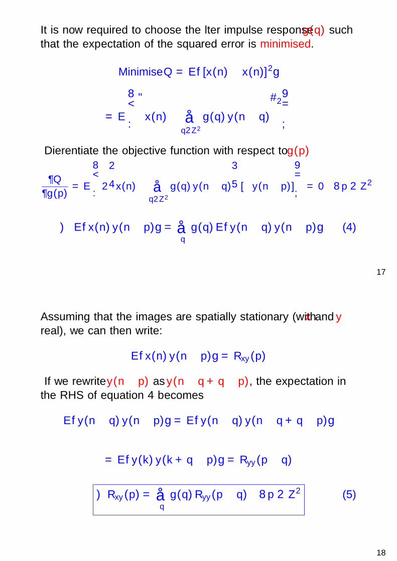
It is now required to choose the filter impulse response g(q) suchthat the expectation of the squared error is minimised.
Minimise Q = E[x(n)− x(n)]2
= E
[x(n)− ∑
q∈Z2
g(q) y(n− q)
]2Differentiate the objective function with respect to g(p)
∂Q
∂g(p)= E
2
x(n)− ∑q∈Z2
g(q) y(n− q)
[−y(n− p)]
= 0 ∀ p ∈ Z2
∴ Ex(n) y(n− p) = ∑q
g(q)Ey(n− q) y(n− p) (4)
17
Assuming that the images are spatially stationary (with x and yreal), we can then write:
Ex(n) y(n− p) = Rxy (p)
If we rewrite y(n− p) as y(n− q + q− p), the expectation inthe RHS of equation 4 becomes
Ey(n− q) y(n− p) = Ey(n− q) y(n− q + q− p)
= Ey(k) y(k + q− p) = Ryy (p− q)
∴ Rxy (p) = ∑q
g(q)Ryy (p− q) ∀ p ∈ Z2 (5)
18

These are the Normal or Wiener-Hopf equations and can, inprinciple, be solved for filter impulse response g(q). Take the FTof this equation
∑p∈Z2
Rxy (p)e−jωT p = ∑
p∈Z2
∑q
g(q)Ryy (p− q)
e−jω
T p
= ∑q
g(q)∑p
Ryy (p− q) e−jωT p
Let p− q = k, and write the FTs of Rxy and g(q) as Pxy (ω) andG (ω) then:
Pxy (ω) = ∑qg(q)∑
k
Ryy (k) e−jωT (q+k) = ∑
qg(q) e−jω
T q ∑k
Ryy (k) e−jωT k
∴ Pxy (ω) = G (ω)Pyy (ω) =⇒ G (ω) =Pxy (ω)
Pyy (ω)
This is the optimum linear filter for recovering the original imagex(n) from the noisy measurements y(n). Note that we mustestimate Pxy from the data. 19
Uncorrelated observation noise
Consider W-H equations when the observation noise d(n) isuncorrelated with the image.
Ryy (p) = Ey(n) y(n−p) where y(n) = ∑m
h(m) x(n−m)+d(n)
If signal and noise are uncorrelated and noise is zero mean:
Ryy (p) = E
∑m
∑qh(m) x(n−m) h(q) x(n− p− q)
+E d(n) d(n− p)
= ∑m
∑q
h(m) h(q)E x(n−m) x(n− p− q)+ Rdd (p)
∴ Ryy (p) = ∑m
∑q
h(m) h(q)Rxx (p + q−m) + Rdd (p)
as
E x(n−m)x(n− p− q) = E x(n−m)x(n−m− (p + q−m))20

Now take the Fourier transform of each side to give:
Pyy (ω) = ∑p
∑m
∑q
h(m) h(q)Rxx (p + q−m)
e−jω
T p +Pdd (ω)
where Pdd is the FT of the autocorrelation function of the noise.Interchange order;
Pyy (ω) = ∑m
∑q
h(m) h(q) ∑p
Rxx (p + q−m) e−jωT p + Pdd (ω)
Let k = (p + q−m), then:
Pyy (ω) = ∑m
∑q
h(m) h(q) ∑k
Rxx (k) e−jωT (k−q+m) + Pdd (ω)
∴ Pyy (ω) =
∑m
h(m) e−jωT m
∑q
h(q) e jωT q
∑k
Rxx (k) e−jωT k
+ Pdd (ω)
∴ Pyy (ω) = |H(ω)|2 Pxx (ω) + Pdd (ω) (6)
as h is real.21
The other term in the Wiener-Hopf equation is:
Rxy (p) = Ex(n) y(n− p)
= E
[∑m
h(m) x(n− p−m) + d(n)
]x(n)
The image x(n) and the noise d(n) are uncorrelated and the noisehas zero mean (as before):
∴ Rxy (p) = E
∑m
h(m) x(n− p−m) x(n)
= ∑
m
h(m)E x(n) x(n− [p + m])
= ∑m
h(m)Rxx (p + m)
22

Taking the Fourier transform of each side gives:
Pxy (ω) = ∑p
∑m
h(m)Rxx (p + m)
e−jω
T p = ∑m
h(m) ∑pRxx (p+m) e−jω
T p
Let p + m = k, then:
= ∑m
h(m) e jωT m ∑
k
Rxx (k) e−jωT k
∴ Pxy (ω) = H∗(ω)Pxx (ω)
Substituting back into the W-H equation gives:
G (ω) =H∗(ω)Pxx (ω)
|H(ω)|2 Pxx (ω) + Pdd (ω)(7)
This is the most commonly used form of the Wiener Filter.
23
NOTES on the Wiener Filter
1. At frequencies where:
|H(ω)|2 Pxx (ω) Pdd (ω)
the Wiener filter becomes the inverse filter 1/H(ω).
2. If the noise is large there will be little deconvolution (ie.inverse filtering)
3. If the blurring function is unity (ie no blurring) then theWiener filter simply recovers the image from the noise; thefilter frequency response is then:
G (ω) =Pxx (ω)
Pxx (ω) + Pdd (ω)
24

NOTES continued
We should also address the question of how one might actually goabout estimating Pxx (the power spectrum of the original image)and Pdd (the power spectrum of the noise).
1. to estimate Pdd we might choose a section of the imagewhich is effectively featureless and form its power spectrum –we are then forming the PS of the noise. Generally this workswell in many cases (note that if we have white noise thepower spectrum, Pdd , is constant).
2. estimating Pxx is clearly harder as we are actually trying torecover the real image – so what might we do in practice?One common method is to approximate Pxx with a constant,K . K can be chosen interactively to produce the empiricallybest results.
25
The FIR Wiener Filter
Note, in general, we get a filter with an infinite region of support.Can derive an FIR approximation but this would not be theoptimum FIR filter.
Repeating derivation of W-H equations shows that they are alsovalid for a finite support region RG :
Rxy (p) = ∑q
g(q)Ryy (p− q) ∀ p, q ∈ RG
Specifically if the region of support is:RG = p1, p2; −M ≤ p1 ≤ M, −M ≤ p2 ≤ M the filter has(2M + 1)2 taps or impulse response coefficients and W-Hequations are
26

Rxy (p1, p2) =M
∑q2=−M
M
∑q1=−M
g(q1, q2)Ryy (p1 − q1, p2 − q2)
∀ p ∈ −M ≤ p1 ≤ M, −M ≤ p2 ≤ M
Can express in matrix form and solve for the filter weightsg(q1, q2) if we can estimate Rxy (and perhaps measure Ryy ).
27
Results
Blurred image + noise
Figure 7: Blurred image with smalladditive noise
Restored image
Figure 8: Image restored by Wienerfilter
28

Blurred image + noise
Figure 9: Blurred image withincreased additive noise
Restored image
Figure 10: Image restored by Wienerfilter
29
It is apparent that the Wiener filter only works well when there is asmall amount of noise – if the image is significantly noisy themethod does not provide sufficient regularisation resulting inartefacts in the restored image.
Note that the above images have been created using the Wienerfilter where Pxx and Pdd were known because we had knowledge ofboth our original image and our noise – in cases where we do nothave this knowledge, we must form the Wiener filter usingestimated values of Pxx and Pdd , and the results are generally poor.
30

Despite the often poor results of the Wiener filter when used onimages which have significant blurring and noise, it is one of thebasic image processing techniques which has provided a startingpoint for many more sophisticated methods.
We showed that the Wiener filter was the optimal filter, why thenis its performance so poor? The answer is that it is optimal overthe space of linear filters, we will show that by extending our spaceto non-linear filters, we can often do much better.
316 SAMPLE RECONSTRUCTIONS FROM THE INVENTORSOriginal Image Blurred and Noisy Image
Pixon Result Wiener Result
Figure 7: Comparison of the performance of the Pixon method to Wiener FilteredFourier Deconvolution for the famous \Lenna" test image. The original image hasbeen blurred with a Gaussian blurring function with an FWHM of 6 pixels beforebeing added with Gaussian noise.29Figure 11: Page taken from The Pixon Method of Image Reconstruction
R. C. Puetter & A. Yahil, in Astronomical Data Analysis Software andSystems VIII, D. M. Mehringer, R. L. Plante & D. A. Roberts, eds., ASPConference Series, 172, pp. 307-316, (1999).
J. Lasenby (2016)
32

IIB 4F8: Image Processing and Image CodingHandout 6 : Image Deconvolution cont. and Image
Enhancement
J Lasenby
Signal Processing Group,Engineering Department,
Cambridge, UK
Lent 2016
1
Spectral Estimation
We note that the Wiener filter relies on the fact that we know orcan accurately estimate the power spectra of the original signaland the noise, Pxx and Pdd .
A reasonable estimate of the power spectrum of the noise canoften be achieved by isolating a portion of the image that we thinkcontains only noise (for example where the original signal isuniform, if such a region exists)
– we can then take the FT of that region (suitably windowed) andform the power spectrum from |FT |2.
2

Estimating the power spectrum of the signal is not such a simplematter; one method would be as follows: assume we haveestimated Pdd .
y(n) = Lx(n) + d(n)
then taking FTs gives
Y (ω) = H(ω)X (ω) +D(ω)
where H = FT (L). Thus, if we have an estimate of D, we canestimate Y −D to be approximately the FT of the signal. Or, ifour blurring function is known we can obtain a better estimate ofX by pseudo-inverse filtering, i.e.
X (ω) =Y (ω)−D(ω)
Hg (ω)
where Hg is the pseudo-inverse filter formed from H (handout 5).
3
What we would really like is an iterative method whereby we couldmake initial guesses/estimates of our signal and noise powerspectra, do the deconvolution and then from the results (looking atresiduals etc.) modify our power spectra estimates.
However, since the Wiener filter is a linear method, it does notlend itself to such an iterative minimisation
– to do a better job we need to go to non-linear filters. By way ofintroduction to one of the main types of non-linear methods, wenow look at deriving the Wiener filter from a Bayesian perspective.
4

Bayesian derivation of Wiener Filter
Now sketch an alternative derivation of the Wiener filter – can thenextend the method to indicate how we might construct non-linearfilters which will do a much better job than the Wiener filter.
Suppose, as before, that our observed image, y , the original image,x , the linear distortion L, and the noise d , are related by
y(n) = Lx(n) + d(n)
Write this equation in vector form –
y = Lx + d
For simplicity in the derivations we shall assume that E [x] = 0 andE [d] = 0, i.e. that both the signal and the noise are zero mean.
5
To find an estimate of x, we choose to maximise Pr(x|y), i.e. theprobability of the original image given the observed data. Whendealing with conditional probabilities we use Bayes’ Theorem:
Pr(x|y) = 1
Pr(y)Pr(y|x)Pr(x)
sometimes also written as Pr(x|y)Pr(y) = Pr(y|x)Pr(x). Inwords we write
Posterior probability =1
evidence[likelihood][prior probability]
Can regard Pr(y), the probability of the data, simply as anormalising factor, which therefore implies that we wish tomaximise
Pr(x|y) ∝ Pr(y|x)Pr(x)
6

Assume gaussian noise (although there is no problem in including aknowledge of the noise – for example, Poisson noise is common inoptical problems – we will here derive our equations for gaussiannoise). Can write the probability of the noise, which is proportionalto the likelihood as
Pr(y|x) ∝ e−12dTN−1d = e−
12 (y−Lx)TN−1(y−Lx)
where N = E [ddT ] is the noise covariance matrix. The dTN−1dterm is the vector equivalent of the 1
σ2 term in the 1d gaussian – if
N is diagonal then N−1 will be diagonal with elements 1σ2i
.
Usually write
Pr(y|x) ∝ e−12χ2
where χ2 = (y− Lx)TN−1(y− Lx).
7
Now have to decide on the assignment of the prior probabilityPr(x) – this probability incorporates any prior knowledge we mayhave about the distribution of the data.Assume an ideal world in which x is a gaussian random variable,described by a known covariance matrix C = E [xxT ] so that
Pr(x) ∝ e−12xTC−1x
Thus we can now write the posterior probability as
Pr(x|y) ∝ Pr(y|x)Pr(x) ∝ e−12 (χ
2+xTC−1x)
which one must maximise wrt x to obtain the reconstruction.This is equivalent to minimising F = 1
2 (χ2 + xTC−1x) .
8

In fact, completing the square in x enables us to write the posterioras
Pr(x|y) ∝ e−12 (x−x)TM−1(x−x) (1)
where
x = W y = the image reconstruction
W = (C−1 + LTN−1L)−1LTN−1 (2)
this is in fact the Wiener filter matrix! and
M = (C−1 + LTN−1L)−1 (3)
is the reconstruction error matrix E [(x− x)(x− x)T ].
9
Below we verify that the above results are correct by firstsubstituting for W into equation 1
(x−W y)TM−1(x−W y) = xTM−1x− xTM−1W y− yTWTM−1x+ yTWTM−1W y(4)
Now show that the terms containing x in the above can beequated to the terms containing x in F
F = (yT − xTLT )N−1(y− Lx) + xTC−1x
This implies that
xTM−1x = xTLTN−1Lx + xTC−1x
Verifying thatM = (C−1 + LTN−1L)−1 (5)
10
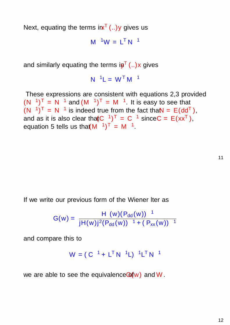
Next, equating the terms in xT (..)y gives us
M−1W = LTN−1
and similarly equating the terms in yT (..)x gives
N−1L = W TM−1
These expressions are consistent with equations 2,3 provided(N−1)T = N−1 and (M−1)T = M−1. It is easy to see that(N−1)T = N−1 is indeed true from the fact that N = E (ddT ),and as it is also clear that (C−1)T = C−1 since C = E (xxT ),equation 5 tells us that (M−1)T = M−1.
11
If we write our previous form of the Wiener filter as
G (ω) =H∗(ω)(Pdd (ω))−1
|H(ω)|2(Pdd (ω))−1 + (Pxx (ω))−1
and compare this to
W = (C−1 + LTN−1L)−1LTN−1
we are able to see the equivalence of G (ω) and W .
12

Thus we have recovered the optimal linear method via a Bayesiananalysis whereas previously we had obtained it by minimisingresidual variances.
Now note the remarkable feature of this: original problem was
y = Lx + d
In general L will not be invertible. e.g. may be a blurring (beam)function in which higher spatial frequencies are strongly suppressed.
However, the estimate x = W y can still be computed no matterhow singular L is — only needs LT to be evaluated!
This is an example of Regularization.
Notice how if the C−1 were not present in W we would just haveW = L−1 [since with no C−1 we can writeW = (LTN−1L)−1(LTN−1L)L−1 = L−1]
— we say we have regularized the inverse; effectively we haveadded on another term in order to avoid singlularities.
13
Maximum Entropy Method (MEM) deconvolution
The Wiener solution is ‘easy’ to calculate and has knownreconstruction errors. However, it is certainly by no means the bestin real problems. It depends on the assumption of gaussianity andknowledge of the covariance structure a priori.
Since the world this not so simple, we are forced to consideralternative priors. One such prior which has been widely andsuccessfully used is the entropy prior.
Usually MEM is applied to positive, additive distibutions (PADS).Let x be the (true) pixel vector we are trying to estimate. Aconsideration of the following general conditions;
• subset independence• coordinate invariance• system independence
leads to the following prior.....14

Pr(x) ∝ eαS
where the cross entropy S of the image is given by
S(x, m) = ∑i
[xi −mi − xi ln
(ximi
)]where m is the measure on an image space (the model) to whichthe image x defaults in the absence of data. (Can see globalmaximum of S occurs at x = m.)
Must then maximise the posterior distribution with the aboveentropic prior for Pr(x).
As this is a complicated non-linear equation, the optimization mustbe performed via some sort of iterative technique. The results areoften impressive and the MEM method has been used extensivelyin astronomy, medical imaging and general image processing.
15
The Pixon Method
The Pixon method is another recently established deconvolutiontechnique – derived initially to deconvolve astronomical images.
We will not look at this in any detail but will state that it can alsobe derived in a Bayesian manner as outlined above using a differentprior. The aim of the pixon method is to first find a distribution ofpixons across the image – a pixon is a box of varying size, thesmallest being a single pixel. We will have large pixons where theimage has little detail and small pixons where there is fine detail.
These pixons are then our basis elements of our image and we setup and minimise our posterior distribution in terms of them. Theresults of the Pixon method have been very impressive (but notethat when the figures below compare with MEM it is generally apoor version of MEM).
16

Figure 1: A comparison of three deconvolution techniques on simulateddata
Figure taken fromhttp://casswww.ucsd.edu/personal/puetter/pixonpage.html.
17
Figure 2: The Pixon method deconvolution of galaxy data
Figure taken fromhttp://casswww.ucsd.edu/personal/puetter/pixonpage.html.
18

Figure 3: The Pixon method deconvolution of x-ray data
Figure taken fromhttp://casswww.ucsd.edu/personal/puetter/pixonpage.html.
19
Figures 1,2,3 show various applications of the Pixon method onreal and simulated images. Figure 1 is particularly interesting as itshows that the pixon reconstruction not only produces a goodlikeness of the original, but also produces residuals which appear tohave the same statistics as the added noise.
Looking at the statistics of the residuals is a very good way ofdetermining how well the deconvolution technique is performing(although in practice we may not of course know the statistics ofthe noise). We would like to see as little structure in the residualsas possible.
20

The hardest deconvolution is blind deconvolution when we do notknow the point spread function.
This can be attacked in a number of ways. In MEM and Pixontechniques we can assume a form for the PSF but give it a variablewidth (e.g. gaussian with a variance which becomes a parameterwe search over).
Another ‘recent’ development in blind deconvolution is theensemble learning method – this too adopts a Bayesian approachand can produce impressive results (if interested see Miskin andMackay, Ensemble learning for blind image separation anddeconvolution. Advances in independent component analysis, (EdGirolami), Springer Verlag, July 2000).
21
Compressed Sensing – in a compressed form
A currently very fashionable area of Signal Processing is known ascompressed sensing.
Look briefly at what this is:
• Suppose we have underlying real data x and that x is sparse insome basis
• Let x be the sparse representation in some basis Ψ, x = Ψx.
• Take another random or incoherent basis Φ, and formy = Φx.
• Task is to reconstruct the signal x from theserandom/incoherent projections
22
Compressed Sensing, continued
• We look for the sparsest solution – the x for the smallest l0norm. But this is hard.
• Some clever maths then tells us we can recover the signal viaminimising the l1 norm
• ...and if we do this, and if some conditions are satisfied, werecover the original signal with high probability.
• So, this seems as though we can redefine our sampling criteriaif we know something about our signal.
• But very little to date which is impressive in the deconvolutionof images field using compressed sensing.
23
Contrast
Consider the illustrations in the figure.
0 100 200 300
0
50
100
150
200
250
3000 100 200 300
0
50
100
150
200
250
300
Figure 4: Illustration of contrast: inner squares have equalluminances/intensities but do not appear equally bright
24

Now consider the figure below:
0 100 200 300
0
50
100
150
200
250
3000 100 200 300
0
50
100
150
200
250
300
Figure 5: Illustration of contrast: inner squares have unequalluminances/intensities but appear equally bright
25
Weber’s Law states that for the intensity of an object, f0 to besuch that it changes from being indiscernible from the backgroundto just noticeably different to the background, which has intensityfb, the ratio of the difference to the object’s intensity must be of aparticular constant value
|fb − f0|fo
= constant
If f0 = f and fb = f + ∆f where ∆f is the small change toproduce the noticeable difference in intensity, then
∆f
f' d(log f ) = ∆c
since d(log f )df = 1
f . ∆c is a constant (empirically taking value of0.02).
26

Previous equation =⇒ equal increments in the log of theintensity should be perceived as equal increments in contrast(∆(log f ) ∝ ∆c).
Thus dcd log f = k1, k1 constant, so that
c = k1 log f + k2
This is the logarithmic law of intensity to contrast. The otherwidely used law is a power law, where the relationship between thecontrast and the intensity can be written as
c = αnf1n or f ∝ cn
where n is often taken to be 3.
27
Histogram Equalisation
In some cases images may exhibit poor use of the available greylevels; may result from poor illumination of the scene ornon-linearity in the imaging system.
To examine this, plot a histogram of frequency of occurrence ofgrey level against grey level as shown below.
white black
Grey level
Number ofoccurences
Here most of the image pixels are concentrated around themid-range grey levels and little use is made of the extreme blackand white levels. 28

An intuitively appealing idea would be to apply a transformation ormapping to the image pixels such that the probability ofoccurrence of the various grey levels should be constant
i.e. all grey levels are equiprobable, which would correspond to aconstant amplitude histogram.
Assume that the image pixel levels are mapped by the function
y = g(x)
where x is an image pixel level and y is the transformed level.
Let the probability density of the pixels in the image be pX (x) andthe probability density of the output image be pY (y). (X ,Y ,random variables).
29
Note that the probability of X lying between x and x + δx , mustbe the same as the probability of g(X ) = Y lying between y andy + δy ,
Xx x+dx
p (x)X
y =g(x)
yy+dy
Figure 6: Sketch showing the equivalence of probabilities over intervals inthe original and transformed frames.
30
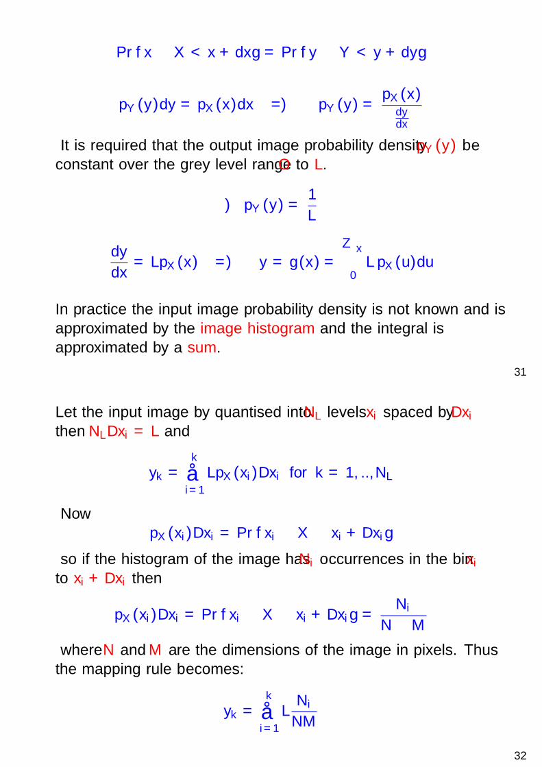
Pr x ≤ X < x + dx = Pr y ≤ Y < y + dy
pY (y)dy = pX (x)dx =⇒ pY (y) =pX (x)
dydx
It is required that the output image probability density pY (y) beconstant over the grey level range O to L.
∴ pY (y) =1
L
dy
dx= LpX (x) =⇒ y = g(x) =
∫ x
0L pX (u)du
In practice the input image probability density is not known and isapproximated by the image histogram and the integral isapproximated by a sum.
31
Let the input image by quantised into NL levels xi spaced by ∆xithen NL∆xi = L and
yk =k
∑i=1
LpX (xi )∆xi for k = 1, ..,NL
NowpX (xi )∆xi = Pr xi ≤ X ≤ xi + ∆xi
so if the histogram of the image has Ni occurrences in the bin xito xi + ∆xi then
pX (xi )∆xi = Pr xi ≤ X ≤ xi + ∆xi =Ni
N ×M
where N and M are the dimensions of the image in pixels. Thusthe mapping rule becomes:
yk =k
∑i=1
LNi
NM
32

Note that if k = NL, yNL= L as required. This may be considered
as a look-up table –i.e. the above values of yk are formed andstored so that we can scan our image x and when the value ofpixel i in x falls within the kth greylevel bin, we map it to yk .
Practical Notes
1. Matlab has a function hist which will perform the histogramoperation and a function cumsum which forms the cumulativesum required in evaluating the mapping.
2. If relatively few bins are used for the histogram then thelook-up table may require interpolation to give a smootherfunction.
33
Figure 7: Image with poor distribution of brightness levels
34

In figure 7 we have the Lenna image with a poor distribution ofbrightness levels. This image has been formed by contrast mappingaccording to the following formula:
y = f (x) = k + sign(x − k)|x − k |[|x − k |
a
]pwhere k = 1
2 (xmin + xmax ) is the average value of the imageintensity, a = 1
2 (xmax − xmin) and sign is +1, 0,−1 if (x − k) ispositive, zero or negative.The exponent p was taken as 2. Note that this mapping preservesboth the maximum, minimum and average values of the image.
35
Figure below shows the previous figure after histogram equalisationusing 64 greylevels. We can see that the greylevels have been’evened out’ so that the image is now more aesthetically pleasing.
Figure 8: Contrast mapped Lenna image with Histogram Equalisation36

Example: Taken from Part IIB Tripos 2006
2. (a) Explain, qualitatively, the concept of histogram equalisation inimages. In what situations would histogram equalisation be useful? [10%]
Assuming that we have a range of greyscale values from 1 to 8, considerthe 4× 4 image given in figure 6
1 1 2 2
3 2 4 3
2 4 3 2
2 3 1 1
Sketch and comment on the histogram of this image.Perform histogram equalisation on this image by finding the set oftransformed values yk, k = 1, .., 8 onto which the original greylevelsare mapped.
Sketch the new equalised image and its histogram, commenting on how
well the process has worked. [40%]
37
Median FilteringMedian filtering is essentially a method for detecting and replacingpixels which are “unlikely” in some sense.
Each pixel in the image is replaced by the median value of thepixels in a window containing the pixel under consideration. If theinput image is x(n1, n2) then the median filtered image y(n1, n2) isgiven by:
y(n1, n2) = medianm1,m2∈Rw
x(n1 −m1, n2 −m2)
where Rw is the support region for the median filter.
38

The window is scanned over the whole image and the pixelx(n1, n2) at the centre of the window is replaced by the medianvalue of the pixels contained in the window surrounding pixelx(n1, n2).To form the median, order window pixels in ascending (ordescending) brightness and choose centre value.e.g. if the pixel values were as shown below, then the pixel at thecentre of the window, value 7, would be replaced with a level of 3which is the median.
39
Figure 9: Image with binary valued impulsive noise
Note that this type of degradation can be performed by the Matlabcommand J = imnoise(I,‘salt & pepper’, D), where binary valuednoise is added to image I at a noise density of D to form new image J.
40

Figure 10: Image after median filtering with 3× 3 window
Figure 10 shows the previous image after application of a median filter
with 3× 3 window. Note that the impulsive noise has disappeared but
that there is a loss of detail due to the smoothing effects of the filter.41
The 2d z-transform
We have discussed the 2d Fourier transform in some detail.However, we should note that the FT converges uniformly only forstable sequences. As an illustration, let us look at the 1d unit step:h(t) = 1 if t ≥ 0, h(t) = 0 if t < 0.
H(ω) =∫ +∞
−∞h(t)e−jωtdt =
∫ ∞
0e−jωtdt
which does not converge. Thus the spectrum of the step functioncannot rigorously be expressed as a FT.The z-transform converges for a much wider class of signals – it isalso very useful (as you will have seen in the 3rd year courses) instudying difference equations and stability.
42

The 2d z-transform of an image or 2d function x(u1, u2) is denotedby X (z1, z2) and defined as a straightforward extension of the 1dz-transform as
X (z1, z2) =+∞
∑n1=−∞
+∞
∑n2=−∞
x(n1, n2)z1−n1z2
−n2
where z1 and z2 are complex variables. The space of (z1, z2) istherefore 4-dimensional. It is easy to see that if we restrict zi to lieon the unit circle, i.e. zi = ejωi , then the z-transform reduces tothe Fourier transform:
X (z1, z2)|z1=ejω1 ,z2=ejω2 =+∞
∑n1=−∞
+∞
∑n2=−∞
x(n1, n2)e−jn1ω1e−jn2ω2 = FT (ω1, ω2)
the z-transform is therefore a generalisation of the Fouriertransform. The 2d surface in the 4d space on which the FT lies(zi = ejωi ) is called the unit surface.
43
An important concept when looking at z-transforms is that of theregion of convergence or RoC.Consider evaluating X (z1, z2) along zi = rie
jωi , where ri , ωi areradius and argument in the zi planes. So, we therefore have
X (z1, z2)|zi=riejωi = ∑
n1∑n2
x(n1, n2)r−n11 r−n22 e−jn1ωi e−jn2ωi
which we recognise as the FT of x(n1, n2)r−n11 r−n22 .
Recall that uniform convergence of our FT, FT (ω1, ω2), requiresthe absolute summability of x(n1, n2), i.e.
∑n1
∑n2
|x(n1, n2)| < ∞
44

An absolutely summable sequence is a stable sequence: stableimplies; bounded input =⇒ bounded output.Similarly, uniform convergence of the z-transform requires theabsolute summability of x(n1, n2)r
−n11 r−n22 , i.e.
∑n1
∑n2
|x(n1, n2)|r−n11 r−n22 < ∞
absolute summability will therefore depend upon the values of r1and r2.
45
One of the motivations for studying the z-transform is that it is auseful tool for the investigation of discrete-time, sampled datasystems. In particular, it easily handles up and down sampling. Toillustrate this look at the 1d z-transform of a signal x(n);
X (z) =+∞
∑n=−∞
x(n)z−n
Since X (z12 ) = ∑+∞
n=−∞ x(n)z−n2 and
X (−z 12 ) = ∑+∞
n=−∞ x(n)(−z)− n2 , then we can see that
1
2
(X (z
12 ) + X (−z 1
2 ))
contains only the even terms, so that
1
2
(X (z
12 ) + X (−z 1
2 ))=
+∞
∑n=−∞
x(2n)z−n
which is the z-transform of the downsampled signal.46
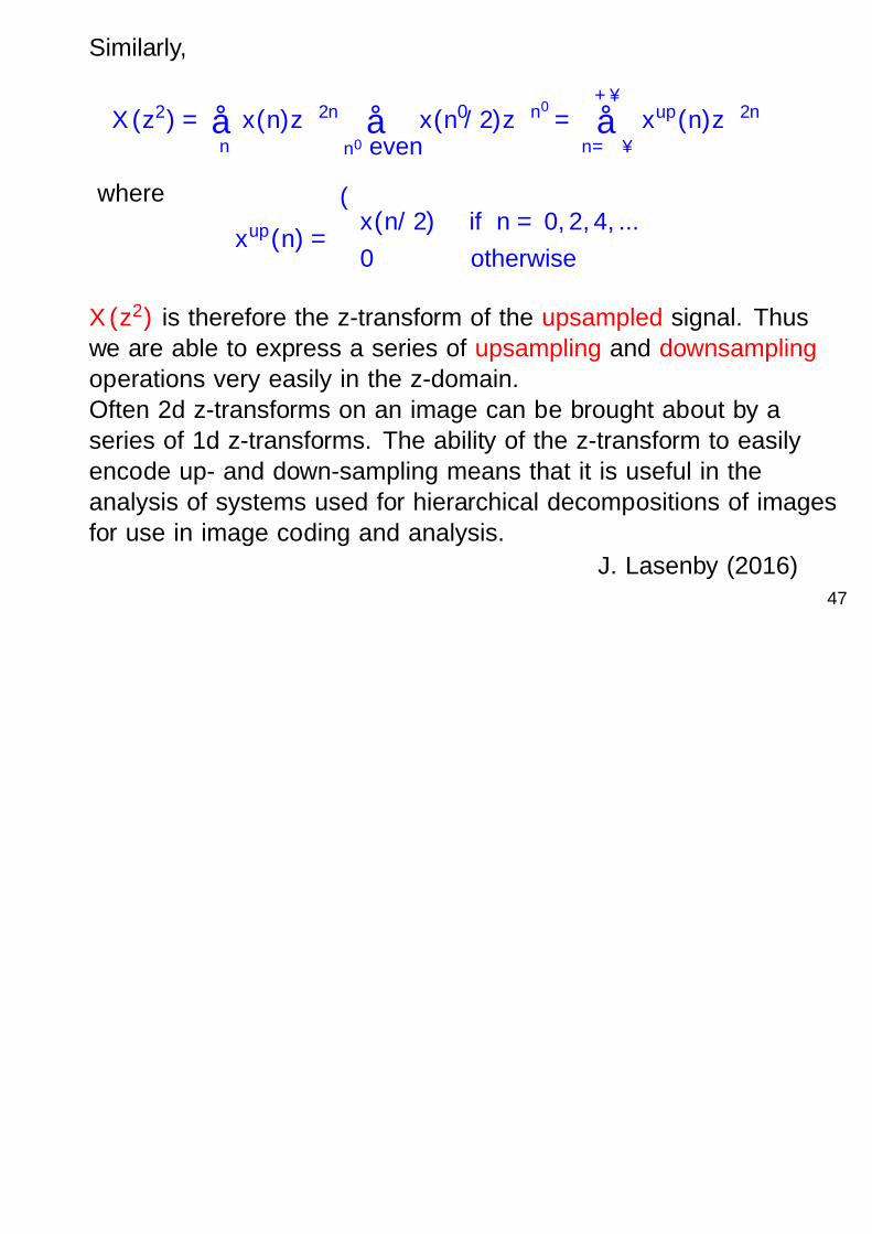
Similarly,
X (z2) = ∑n
x(n)z−2n ∑n′ even
x(n′/2)z−n′=
+∞
∑n=−∞
xup(n)z−2n
where
xup(n) =
x(n/2) if n = 0, 2, 4, ...
0 otherwise
X (z2) is therefore the z-transform of the upsampled signal. Thuswe are able to express a series of upsampling and downsamplingoperations very easily in the z-domain.Often 2d z-transforms on an image can be brought about by aseries of 1d z-transforms. The ability of the z-transform to easilyencode up- and down-sampling means that it is useful in theanalysis of systems used for hierarchical decompositions of imagesfor use in image coding and analysis.
J. Lasenby (2016)47