Embed Size (px)
Citation preview

IVEware: Imputation and VarianceEstimation Software
(Version 0.3) 1
T. RaghunathanP. SolenbergerP. Berglund
J. van HoewykUniversity of MichiganAnn Arbor, Michigan
1 c© The Regents of the University of Michigan, 2016. All rights reserved. Permission is grantedto use, copy and redistribute this software for any purpose, so long as no fee is charged and solong as the copyright notice above, this grant of permission, and the disclaimer below appear in allcopies made; and so long as the name of the university of michigan is not used in any advertisingor publicity pertaining to the use or distribution of this software without specific, written priorauthorization. Permission to modify or otherwise create derivative works of this software is notgranted. This software is provided as is, without representation as to its fitness for any purpose, andwithout warranty of any kind, either express or implied, including without limitation the impliedwarranties of merchantability and fitness for a particular purpose. The regents of the University ofMichigan shall not be liable for any damages, including special, indirect, incidental, or consequentialdamages, with respect to any claim arising out of or in connection with the use of the software,even if it has been or is hereafter advised of the possibility of such damages.

Contents
2

Chapter 1
Basics
1.1 What is IVEware?
IVEware is a collection of routines written under various platforms and packaged to performmultiple imputations, variance estimation and, in general, draw inferences from incompletedata. The software can also be used to perform analysis without any missing data. IVEwaredefaults to assuming a simple random sample, but uses the Jackknife Repeated Replicationor Taylor Series Linearization techniques for analyzing data from complex surveys.
IVEware can be run with SAS, Stata, R, SPSS or as stand-alone under the Windowsor Linux environment. The R, Stata, SPSS and stand-alone version can also be used withthe Mac OS. The stand-alone version has limited capabilities for analyzing the multiplyimputed data though the routines for creating imputations are the same across all packages.The command structure is the same across all platforms. IVEware can be executed using thebuilt-in XML editor or it can be run using the built-in editor within the four software packagespreviously mentioned. The user can also mix and match the codes from these softwarepackages through a standard XML toggle-parser (for example, < SAS name = “myfile” >SAS commands < /SAS > will execute the SAS commands and store the commands in thefile “myfile.sas”.) if the provided XML editor is used to execute IVEware commands.
1.2 Download and Setup
Various versions of IVEware can be downloaded and installed from www.iveware.org. Instal-lation instructions and setup are slightly different for Windows, Linux and MAC operatingsystems, therefore, it is very important to follow the instructions for IVEware to work prop-erly.
1.2.1 Windows
Download the file srclib windows.exe and double click on it to install. By default, all therelevant software files are extracted to the directory
C:\Program Files (x86)\srclib
3

4 CHAPTER 1. BASICS
You may change the directory and the location you choose will then replace
~/srclib
in the guides given later to make IVEware work with one or more packages SAS, SPSS,Stata, and R. The installer will create a desktop icon unless you choose not to.
The next step is make sure that IVEware can execute the appropriate software. Find thepath of the directory where the executable file of the software is located. For example, thetypical location of the file “sas.exe” to run SAS version 9.4 is,
C:\Program Files\SASHome2\SASFoundation\9.4\sas.exe
Similarly, a 64-bit executable “Rgui.exe’ may be located in
C:\Program Files\R\R-3.2.3\bin\x64\Rgui.exe
Find the path of the other software executable files, if needed.Next edit the file “settings.xml” in the “srclib” directory. Here is an example of a file
appropriate to run IVEware with all four software (SAS, R, Stata, and SPSS) packages:
<settings>
<frameworks>
<sas path="C:\Program Files\SASHome2\SASFoundation\9.4\sas.exe" />
<spss path="C:\Program Files\IBM\SPSS\Statistics\22\stats.exe" />
<stata path="M:\stata14SE-64bit\StataSE-64.exe" />
<R path="C:\Program Files\R\R-3.2.3\bin\x65\Rgui.exe" />
<gnuplot path="C:\Program Files\gnuplot\bin\wgnuplot.exe" />
</frameworks>
</settings>
In this example, the Stata executable file is located in the network drive M :. The stand-alone version uses ”GNUPLOT” for creating and displaying graphics. You should downloadand install this package. For more details about this software, see www.gnuplot.info.To verify that IVEware is correctly installed, download the example file
ive examples windows.zipand extract it to the directory of your choice (for example, create a subdirectory callediveware under the Documents directory). Double click the IVEware icon which will openan XML editor window. Choose “File”, navigate to the directory with the example files,choose any example XML file to open, and click “Run”. You can also run IVEware in batchmode by typing:
"C:\Program Files (x86)\srclib\srcexec" ive_example_file.xml
in the command window after setting the current directory to the directory where the ex-ample file is located. Use MS Word or another software to check the “*.log” files producedby the run to see that there were no errors and also compare the “*.lst” files produced byrun with the corresponding “*.chk” files. They should differ only in the dates.

1.2. DOWNLOAD AND SETUP 5
1.2.2 Linux
For installing IVEware on a Linux system, download the file “srclib pclinux64.tgz” fromwww.iveware.org and extract the srclib directory into an appropriate parent directory, suchas, “/usr/local/” or in your home directory. You can copy the files into the subdirectory ofyour choice. The location you choose will replace ‘∼ /srclib” in guides for using IVEwarewith R, SAS, SPSS, Stata and Srcware, as described in later examples. If you plan to useSrclib with R, SAS, SPSS or Stata and the version cannot be invoked by its lower-case name,edit the “srclib/settings.xml” file to provide the correct path.
As before, you can verify that IVEware is installed correctly by downloading the file“ive examples pclinux.tgz” and extracting the examples directory into an appropriate parentdirectory, for example, the home directory. Navigate to the srclib directory, double-click thesrcshell icon, click File-Open, navigate to the Examples directory, open an appropriate setupfile, for example, “ive examples srcware.xml”, and finally, click Run. You can also run theprogram in batch mode. For example, navigate to the examples directory and use srcexecto run an appropriate setup file:
~/srclib/bin/srcexec ive_examples_sas.xml
where ∼ /srclib is the directory containing IVEware.Use the Linux “cat” and “diff” commands (or other software such as OpenOffice), check
the *.log files produced by the run to see that there were no errors and compare the *.lstfiles produced by run with the corresponding *.chk files. Again, they should differ only inthe dates.
1.2.3 Mac OS
For those using a MAC-OS, IVEware can be used only as stand-alone or with Stata, R andSPSS. For installing IVEware on a Mac OS system, download the file srclib macosx64.tgzfrom www.iveware.org and extract the srclib directory into an appropriate parent directory,such as, “/usr/local/” or in your home directory. You can extract the files into a directoryof your choice. The location you choose will replace “? /srclib” in guides for using IVEwarewith R, SAS, SPSS, Stata and Srcware, as described in later examples. If you plan to useSrclib with R, SAS, SPSS or Stata and the version cannot be invoked by its lower-case name,edit the “srclib/settings.xml” file to provide the correct path.
As before, you can verify that IVEware is installed correctly by downloading the file“ive examples macosx.tgz” and extracting the examples directory into an appropriate parentdirectory, for example, the home directory. Navigate to the srclib directory, double-click thesrcshell icon, click File-Open, navigate to the Examples directory, open an appropriate setupfile, for example, “ive examples srcware.xml”, and, finally, click Run. You can also run theprogram in batch mode. For example, navigate to the examples directory and use srcexecto run an appropriate setup file, for example:
~/srclib/bin/srcexec ive\_examples\_sas.xml
where “∼ /srclib” is the directory containing IVEware.

6 CHAPTER 1. BASICS
Use the MacOS/Linux “cat” and “diff” commands (or other software, such as OpenOffice)to check the “*.log” files produced by the run to see that there were no errors and to comparethe “*.lst” files produced by the run with the corresponding “*.chk” files. They should differonly in the dates.
1.3 Structure of IVEware
IVEware is organized into seven modules to perform various tasks. The six core modules areIMPUTE, BBDESIGN, DESCRIBE, REGRESS, SYNTHESIZE and COMBINEand the seventh module, SASMOD, is specific to SAS.
1. IMPUTE uses a multivariate sequential regression approach (Raghunathan et al(2001), Raghunathan (2015)). This approach is also called Chained Equations, (VanBuuren and Oudshoorn (1999)) and Fully Conditional Specification (Van Buuren (2012))and is used to impute item missing values or unit non-response. IMPUTE can createmultiply imputed data sets and can handle continuous, categorical, count and semi-continuous variables.
2. BBDESIGN implements the weighted finite population Bayesian Bootstrap approachto generate synthetic populations from complex survey data. The primary goal is toincorporate weighting, clustering and stratification in a nonparametric approach forgenerating the non-sampled portion of the population from the posterior predictivedistribution, conditional on the observed data and the design information. For moredetails see Zhou, Elliott and Raghunathan (2015, 2016a, 2016b)
3. DESCRIBE estimates population means, proportions, subgroup differences, contrastsand linear combinations of means and proportions. A Taylor Series Linearizationapproach is used to obtain variance estimates appropriate for a user-specified complexsample design. Multiple imputation analysis can also be performed when there ismissing data.
4. REGRESS fits linear, logistic, polytomous, Poisson, Tobit and proportional hazardregression models. For data resulting from a complex sample design, the JackknifeRepeated Replication technique is used to obtain variance estimates. As in otherIVEware commands, a multiple imputation analysis can be performed when there aremissing values.
5. SYNTHESIZE uses the multivariate sequential regression approach to create full orpartial synthetic data sets to limit statistical disclosure (See Raghunathan, Reiter andRubin (2003), Reiter (2002) and Little, Liu and Raghunathan (2004) for more details.)All item missing values are also imputed when creating synthetic data sets. However,DESCRIBE, REGRESS and SASMOD modules cannot be used to analyze syntheticdata sets as they DO NOT implement the appropriate combining rules. Examples ofimplementation of correct combining rules for synthesized data sets are included inlater sections of this guide.

1.4. HOW TO RUN IVEWARE WITH SOFTWARE PACKAGES? 7
6. COMBINE is useful for combining information from multiple sources through mul-tiple imputation. Suppose that Data 1 provides variables X and Y, Data 2 providesvariables X and Z and Data 3 provides variables Y and Z. COMBINE can be used toconcatenate the three data sets and multiply impute the missing values of X, Y andZ to create large data sets with complete data on all three variables. All item missingvalues in the individual data sets will also be imputed. The multiply imputed combineddata sets can be analyzed using DESCRIBE, REGRESS and SASMOD modules (seeSchenker, Raghunathan, and Bondarenko (2010) for an application and Dong, Elliottand Raghunathan (2014a, 2014b) for more details).
7. SASMOD (requires SAS) allows users to take into account complex sample designfeatures when analyzing data with selected SAS procedures. Currently the followingSAS PROCS can be called: CALIS, CATMOD, GENMOD, LIFEREG, MIXED, NLIN,PHREG, and PROBIT. A multiple imputation analysis can be performed when thereare missing values. Unlike the other IVEware modules, SASMOD requires SAS.
There are many packages such as R (“with”, “mitools”, and “pool”), Stata (“mi esti-mate”), SAS (”PROC MI, PROC MIANALYZE”) to analyze multiply imputed data sets.All these packages can be used within the “XML” structure of IVEware.
1.4 How to run IVEware with software packages?
There are many ways to run IVEware. The choice of how to run the program may dependupon whether the data is stored as a text file or as a software specific file (such as a SAS dataset) or whether to use the Srcshell XML editor bundled with IVEware or use the built-ineditors in specific software package (such as program editor in SAS). IVEware can also berun in batch mode using the command file. Given this level of flexibility, it is not possible tocover every method in detail. Nevertheless, the next few sections provide various examplescenarios which might help users develop code for their own needs and situation. Additionalexamples of running IVEware are provided in later chapters.
This section uses the data from a case control study that was conducted in Seattleand King County to assess the relationship between dietary intake of omega-3 fatty acids(in particular, docosahexaenoic and eicosapentaenoic acids). These fatty acids are mostlyderived from eating fish or seafood. Table 1.1 provides a list of variables and a descriptionof the content. The goal of this example is to perform multiple imputation of the missingvalues.
1.4.1 IVEware and SAS
As explained earlier, IVEware can be run using the provided XML editor or using theRegular Program Editor in SAS (NOT the Enhanced Editor). The XML editorapproach is described first as it is our most preferred approach. This analysis uses datastored in a text file (“mydata2.txt”) with the first row representing the variable names.Create and save an XML file ( the default extension is “.xml”) with the following structure.The commands are explained whenever needed.

8 CHAPTER 1. BASICS
Table 1.1: A list of variables in the data set used in the exampleVariable Description RemarksCASECNT Case-Control Status 1=Case; 0=ControlAGE Age at the time event (case) Continuous
or interview (control)GENDER Gender of the subject 1=Female 0=MaleRACE3 Race of the subject 1=White 0=Non-whiteHYPER Hypertension status 1=Hypertensive
0=Not hypertensiveDIAB Diabetes Status 1=Diabetic 0=Non-diabeticSMOKE Smoking Status 1=Never 2=Former
3=CurrentNUMCIG Number of Cigarettes per week Continuous,
restricted to currentand former smokers
YRSSMOKE Number of years smoked Continuous,restricted to current andformer smokers,must be less than age
FATINDEX Score measuring total Fat intake ContinuousFAMMI History of Family history 1=Yes 0=NoEDUSUBJ3 Education Categories Less than High school,
High school, some Collegeand College
DHA EPA Dietary intake of Omega-3 based Continuouson Food Frequency Questionnaire
REDTOT Red cell membrane Continuousmeasure of Omega-3
CHOLESTH High cholesterol 1=Yes 0=NoCAFFTOT Caffeine intake Semi-continuous or MixedWGTKG Weight in Kilograms ContinuousTOTLKCAL Total Kcal spent on physical activity ContinuousALCOHOL3 Alcohol Intake Semi-continuous or MixedHGTCM Height in centimeters Continuous

1.4. HOW TO RUN IVEWARE WITH SOFTWARE PACKAGES? 9
<sas name="ive_examples">
/* iveware examples - sas version */
/* import the input datasets */
proc import datafile=’mydata2.txt’ out=mydata2 dbms=tab replace;
getnames=yes;
run;
The first line
<sas name="ive_examples">
indicates the beginning of SAS commands which are to be stored in a file called “ive examples.sas”in the current directory (the same directory where the XML file will be stored). The filescalled ive examples.log and ive examples.lst are the corresponding log and list files createdby SAS. The command,
<sas name="ive_examples",dir="c:\mydir">
will store the sas, log and list files in the directory “c:\mydir”.Once the SAS toggle has been invoked, any SAS commands can be inserted including
comments. Here, ”PROC IMPORT” is used to import a text file and create a data set called“mydata2.sas7bdat” in the SAS work directory. The user can provide a full path for thesefilenames and also use libname in SAS to point to the directory containing the data files.
/* run iveware */
/* multiple imputation */
<impute name="impute">
title Multiple imputation;
datain mydata2;
dataout impute;
default continuous;
categorical casecnt gender race3 hyper diab smoke fammi edusubj3 cholesth;
mixed cafftot alcohol3;
transfer studyid;
restrict numcig(smoke=2,3) yrssmoke(smoke=2,3);
bounds numcig(>0) yrssmoke(>0,<=age-12) fatindex(>0) cafftot(>=0) alcohol3(>=0);
maxpred redtot(3) wgtkg(2);
minrsqd .01;
iterations 5;
multiples 5;
seed 2001;
run;
</impute>

10 CHAPTER 1. BASICS
The command
<impute name="impute">
now toggles the beginning of the IMPUTE module and stores commands in a file called“impute.set” in the current directory (that is, directory where the XML file is stored). AllIVEware files (produced by IMPUTE, DESCRIBE, REGRESS, COMBINE and SYNTHE-SIZE) have a “.set” extension. The filenames in “datain” and “dataout” can follow the SASconvention of “libname.sasname” while a libname can be assigned before invoking IMPUTE.For more detail on IMPUTE keywords, see Chapter 2. The line:
</impute>
indicates the closure or end of the IMPUTE commands. Finally, the
</sas>
command indicates the end of all SAS commands. Now, click “run” to execute the program.If you already have a setup file named “impute.set” in the directory, it will be overwritten.
Once you have run the Srcshell, you can reuse the SAS setup file it creates, “ive examples.sas”without Srcshell by issuing the following command
sas ive_examples.sas
in a command window to run in batch mode. Similarly, in the Linux system, you can use
sas ive_examples.sas &
to run the program in background. Suppose that you have a setup file called “previous-run.set” from a previous run then you can rerun it by creating a simpler xml file consistingof the single line:
<impute name="previous" />
and then click ”run”.IVEware can be run interactively in Windows SAS by using the Regular Program Editor
(once again, NOT the Enhanced Editor). First, open or create and save a SAS program(.sas) file and then submit or run it as usual from the editor. This may be an attractiveoption, especially if you are used to running SAS and an earlier version of IVEware. Forexample, the first line in the SAS command file is the following options statement:
options set = SRCLIB ’~/srclib/sas’ sasautos=(’!SRCLIB’ sasautos) mautosource;
where
~\srclib
is the IVEware installation directory.This approach (as opposed to the modification of the SAS configuration file used in the
previous version of IVEware) is easier, especially, when the user does not have write privilegesfor the configuration file (such as with a network installation). The following commands canbe used to perform the same set of tasks as in the XML version discussed above.

1.5. IVEWARE AND R 11
/* iveware examples - sas version */
/* import the input datasets */
proc import datafile=’mydata2.txt’ out=mydata2
dbms=tab replace;
getnames=yes;
run;
/* run iveware */
/* multiple imputation */
%impute(name=impute, dir=. setup=new);
title Multiple imputation;
datain mydata2;
dataout impute;
default continuous;
categorical casecnt gender race3 hyper diab smoke fammi
edusubj3 cholesth;
mixed cafftot alcohol3;
transfer studyid;
restrict numcig(smoke=2,3) yrssmoke(smoke=2,3);
bounds numcig(>0) yrssmoke(>0,<=age-12) fatindex(>0)
cafftot(>=0) alcohol3(>=0);
maxpred redtot(3) wgtkg(2);
minrsqd .01;
iterations 5;
multiples 5;
seed 2001;
run;
Click ”run” to submit the commands. You can modify the program and use the libnameand other SAS features to read data from a different directory, store the output in anotherdirectory, and save and execute the program in some other directory.
1.5 IVEware and R
The structure of running IVEware in the R-package is very similar to running in the SASenvironment as described in the previous section. Using the Srcshell XML editor, you cancreate the following commands.
<R name="ive_examples">
# The above line toggles the beginning of the R commands

12 CHAPTER 1. BASICS
# iveware examples - R version
# import the input datasets
mydata2 <- read.delim("mydata2.txt")
save(mydata2, file="mydata2.rda")
# run iveware
# multiple imputation
<impute name="impute">
title Multiple imputation;
datain mydata2;
dataout impute;
default continuous;
categorical casecnt gender race3 hyper diab smoke fammi
edusubj3 cholesth;
mixed cafftot alcohol3;
transfer studyid;
restrict numcig(smoke=2,3) yrssmoke(smoke=2,3);
bounds numcig(>0) yrssmoke(>0,<=age-12) fatindex(>0)
cafftot(>=0) alcohol3(>=0);
maxpred redtot(3) wgtkg(2);
minrsqd .01;
iterations 5;
multiples 5;
seed 2001;
run;
</impute>
# The line below indicates the end of R-commands
</R>
Click “run” to execute the command. This will create a file called “ive examples.R” withR commands and the “impute.set” file with all needed Impute commands . If you alreadyhave the files with those names, then they will be overwritten.
Some users may prefer to run IVEware fully in the R environment instead of usingthe Srcshell XML editor. Use any text editor to create save an Impute setup file (say,“impute.set” or any other file with a “.set” extension) with the following structure. Thecommand file along with the data file should either be in the same directory or you cansimply provide the full path in the command file.
title Multiple imputation;

1.5. IVEWARE AND R 13
datain mydata2;
dataout impute;
default continuous;
categorical casecnt gender race3 hyper diab smoke fammi
edusubj3 cholesth;
mixed cafftot alcohol3;
transfer studyid;
restrict numcig(smoke=2,3) yrssmoke(smoke=2,3);
bounds numcig(>0) yrssmoke(>0,<=age-12) fatindex(>0)
cafftot(>=0) alcohol3(>=0);
maxpred redtot(3) wgtkg(2);
minrsqd .01;
iterations 5;
multiples 5;
seed 2001;
run;
Next Start R. In the R editor, type the R commands and execute as usual.
# iveware examples - R version
# import the input datasets
mydata2 <- read.delim("mydata2.txt")
save(mydata2, file="mydata2.rda")
# initialize srclib
srclib <<- "~/srclib/R"
source(file.path(srclib, "init.R", fsep=.Platform$file.sep))
# run iveware
# multiple imputation
impute(name="impute")
Use the full path of the actual directory where IVEware is installed for
~/srclib
1.5.1 SPSS and IVEware
Running IVEware with SPSS is slightly different. Use the Srcshell XML editor and type thefollowing commands:

14 CHAPTER 1. BASICS
<spss name="ive_examples">
/* iveware examples - spss version */
/* import the input datasets */
get translate file="mydata2.txt" /type=tab /fieldnames.
save outfile="mydata2.sav".
/* run iveware */
/* multiple imputation */
<impute name="impute">
title Multiple imputation;
datain mydata2;
dataout impute;
default continuous;
categorical casecnt gender race3 hyper diab smoke fammi
edusubj3 cholesth;
mixed cafftot alcohol3;
transfer studyid;
restrict numcig(smoke=2,3) yrssmoke(smoke=2,3);
bounds numcig(>0) yrssmoke(>0,<=age-12) fatindex(>0)
cafftot(>=0) alcohol3(>=0);
maxpred redtot(3) wgtkg(2);
minrsqd .01;
iterations 5;
multiples 5;
seed 2001;
run;
</impute>
</spss>
Click ”run”. When SPSS opens its interactive command window, select ”all” and click the”run” icon to execute the commands.
A successful run of Srcshell with SPSS creates an SPSS setup file called ive examples.spsfor this example. You can modify the file in the future and run without Srcshell by issuingthe following command:
spss ive_examples.sps
Some users may prefer to run using the editor in SPSS without using the Srcshell editor.The following commands illustrate the use of the SPSS editor. Change to the working

1.5. IVEWARE AND R 15
directory and use the SPSS Syntax Editor to create and save an Impute setup file (say,“impute.set”) with the following structure:
title Multiple imputation;
datain mydata2;
dataout impute;
default continuous;
categorical casecnt gender race3 hyper diab smoke fammi
edusubj3 cholesth;
mixed cafftot alcohol3;
transfer studyid;
restrict numcig(smoke=2,3) yrssmoke(smoke=2,3);
bounds numcig(>0) yrssmoke(>0,<=age-12) fatindex(>0)
cafftot(>=0) alcohol3(>=0);
maxpred redtot(3) wgtkg(2);
minrsqd .01;
iterations 5;
multiples 5;
seed 2001;
run;
Using the Syntax Editor, create and save an SPSS setup file (say, “ive example.sps”)with the following commands.
begin program.
import sys
sys.path.insert(0, ’~/srclib/spss’)
import srclib
end program.
/* iveware examples - spss version */
/* import the input datasets */
get translate file="mydata2.txt" /type=tab /fieldnames.
save outfile="mydata2.sav".
/* run iveware */
/* multiple imputation */
begin program.
srclib.impute(name="impute")
end program.
Select ”all” and click the ”run” icon. For

16 CHAPTER 1. BASICS
~/srclib
use the exact path of the installation directory of IVEware.
1.5.2 Stata and IVEware
To run Stata with the Srcshell XML editor, type the following commands:
<stata name="ive_examples">
/* iveware examples - stata version */
/* import the input datasets */
insheet using mydata2.txt, clear names case tab
save mydata2, replace
/* run iveware */
/* multiple imputation */
<impute name="impute">
title Multiple imputation;
datain mydata2;
dataout impute;
default continuous;
categorical casecnt gender race3 hyper diab smoke fammi
edusubj3 cholesth;
mixed cafftot alcohol3;
transfer studyid;
restrict numcig(smoke=2,3) yrssmoke(smoke=2,3);
bounds numcig(>0) yrssmoke(>0,<=age-12) fatindex(>0)
cafftot(>=0) alcohol3(>=0);
maxpred redtot(3) wgtkg(2);
minrsqd .01;
iterations 5;
multiples 5;
seed 2001;
run;
</impute>
</stata>
Click ”run”. Once you’ve run Srcshell, a Stata setup file called “ive examples.do’ iscreated. As with other packages, you can modify the file for future use with any editor andrun using the following commands:

1.5. IVEWARE AND R 17
stata ive_examples.do
As in the case of other software, IVEware can be run using the Stata built-in editor. Todo so, change to the working directory and utilize the Stata do-file editor to create and savean Impute setup file (“impute.set”) with the following structure:
title Multiple imputation;
datain mydata2;
dataout impute;
default continuous;
categorical casecnt gender race3 hyper diab smoke fammi
edusubj3 cholesth;
mixed cafftot alcohol3;
transfer studyid;
restrict numcig(smoke=2,3) yrssmoke(smoke=2,3);
bounds numcig(>0) yrssmoke(>0,<=age-12) fatindex(>0)
cafftot(>=0) alcohol3(>=0);
maxpred redtot(3) wgtkg(2);
minrsqd .01;
iterations 5;
multiples 5;
seed 2001;
run;
In the do-file editor, open or create a Stata setup file with the following structure:
global srclib "~/srclib/stata"
/* iveware examples - stata version */
/* import the input datasets */
insheet using mydata2.txt, clear names case tab
save mydata2, replace
/* run iveware */
/* multiple imputation */
global name "impute"
do $srclib/impute
Click ”run”. As before,
~\srclib
is the name of the IVEware installation directory.

18 CHAPTER 1. BASICS
1.6 How to run IVEware as stand-alone
IVEware can be used as stand-alone software (SRCWARE) for performing multiple impu-tation (using the IMPUTE module) and perform analyses using DESCRIBE, BBDE-SIGN, REGRESS, SYNTHESIZE, or COMBINE, with or without incorporation ofcomplex design features. This section provides example code for reading the data from a textfile and performing multiple imputation. See later chapters for additional examples of codeand output for other analyses/modules. Like other software packages, SRCWARE can berun using the XML editor or through creation of a setup file using any text editor executedin a command window.
First, click on the Srclib icon and choose “File” and “New” to create a new commandfile. The GETDATA module is used to read a text file containing data, and subsequentlyattach variable name, type (character or numeric) and formats (optional). The user canspecify the delimiter as comma (“csv”), space (“\s”), tab (“\t”) etc., and the number ofrows to be skipped prior to reading data from the text file. The following commands readthe example file “myfile2.txt” provided with the software and also described in Section 1.4:
<srcware name=‘‘ive\_examples’’>
/* iveware examples - srcware version */
/* import the input datasets */
<getdata name="mydata2">
data mydata2.txt;
metadata;
delim "\t";
skip 1;
variables
name=STUDYID type=char;
name=CASECNT type=num;
name=AGE;
name=GENDER;
name=RACE3;
name=HYPER;
name=DIAB;
name=SMOKE;
name=NUMCIG;
name=YRSSMOKE;
name=FATINDEX;
name=FAMMI;
name=EDUSUBJ3;
name=DHA_EPA;
name=REDTOT;
name=CHOLESTH;
name=CAFFTOT;

1.6. HOW TO RUN IVEWARE AS STAND-ALONE 19
name=WGTKG;
name=TOTLKCAL;
name=ALCOHOL3;
name=HGTCM;
end;
run;
</getdata>
Note that “skip 1;” instructs GETDATA to skip the first row and the “delim “\t” ” statesthat this is tab-delimited data. The keyword “metadata” begins entering of informationabout the data, and the keyword “variables” indicates the beginning of establishing thename and type of the variables in the columns through use of the keywords “name” and“type”. Finally, “end” closes the entering of metadata. The full extent of what can bespecified under “metadata” keyword is specified below:
metadata
variables
name=gender
type=num
label=‘‘Respondent’s Gender’’
codeframe=sexfmt
location=number
width=number
decimals=number
missing=-9;
codeframe sexfmt 1 male 2 female -9 missing;
end;
The above defines the name, type, label and format of the variable “gender”. For non-delimited data, location number indicates the starting location column number for thevariable and width number specifies the width of the given variable. This feature cannotbe used with delimited data. The default location number is 1 for the first variable. Ingeneral, the location for any variable is the previous variable location plus the width of theprevious variable. Decimals Number is used to specify the number of implicit decimalplaces for the variable. This defaults to 0 for character and non-consecutive variables, andto the previous number of decimals for non-character variables after the first in a series. Themissing data value for the variable is ”.” or any other missing data type of character(s) suchas .N or .J. with a default of none.
Another option is to put the variable names as the first row and use the following codeto read the data set:
<getdata name=‘‘mydata2’’>
table mydata2.txt;
</getdata>
The following code is then used to specify the multiple imputation:

20 CHAPTER 1. BASICS
/* run iveware */
/* multiple imputation */
<impute name=‘‘impute’’>
title Multiple imputation;
datain mydata2;
dataout impute;
default continuous;
categorical casecnt gender race3 hyper diab smoke fammi
edusubj3 cholesth;
mixed cafftot alcohol3;
transfer studyid;
restrict numcig(smoke=2,3) yrssmoke(smoke=2,3);
bounds numcig(>0) yrssmoke(>0,<=age-12) fatindex(>0)
cafftot(>=0) alcohol3(>=0);
maxpred redtot(3) wgtkg(2);
minrsqd .01;
iterations 5;
multiples 5;
seed 2001;
run;
</impute>
</srcware>
To execute, save the file and click “Run’.
1.7 Reading and Writing Other Software Formats
It may be easier to use some other software to write to a file that can be read by IVEware.This section provides some useful commands for importing and exporting data to otherpopular software packages.
1. To write a Gauss data set as a tab-delimited text table that can be read by Srcware,run the following Gauss command:
rc = export(mydata, "mydata.txt", mynames)
To read a tab-delimited text table created by Srcware, run the following Gauss com-mand:
{mydata, mynames} = import("mydata.txt", 0, 1)
2. To write an R data set as a tab-delimited text table that can be read by Srcware, runthe following R command:

1.7. READING AND WRITING OTHER SOFTWARE FORMATS 21
write.table(mydata, file="mydata.txt", na="", row.names=FALSE,
qmethod="double", sep="\t")
To read a tab-delimited text table created by Srcware, run the following R command:
mydata<-read.table("mydata.txt", header=TRUE, sep="\t")
3. To write a SAS data set as a tab-delimited text table that can be read by Srcware,define the library and run the following SAS program:
proc export data=mylib.mydata outfile=’mydata.txt’
dbms=tab replace; run;
To read a tab-delimited text table created by Srcware, define the library and run thefollowing SAS program:
proc import datafile=’mydata.txt’ out=mylib.mydata dbms=tab
replace; getnames=yes; run;
Specify ”-noterminal” in the SAS invocation to export/import delimited data sets innon-interactive command-line mode.
4. To write an S-Plus data set as a tab-delimited text table that can be read by Srcware,define the library and run the following S-Plus command:
write.table(mydata, file="mydata.txt", dimnames.write="col",
na="", sep="\t")
To read a tab-delimited text table created by Srcware, define the library and run thefollowing S-Plus command:
mydata<-read.table("mydata.txt", header=T, row.names=NULL,
sep="\t")
5. To write an SPSS data set as a tab-delimited text table that can be read by Srcware,run the following SPSS command:
save translate outfile="mydata.txt" /type=tab /fieldnames
/replace.
To read a tab-delimited text table created by Srcware, run the following SPSS com-mand:
get translate file="mydata.txt" /type=tab /fieldnames.
The “get” translate function exists only in the Windows implementation of SPSS.

22 CHAPTER 1. BASICS
6. To write a Stata data set as a tab-delimited text table that can be read by Srcware,open the data set in Stata and run the following command:
outsheet using "mydata.txt", replace nolabel
To read a tab-delimited text table created by Srcware, run the following Stata com-mand:
insheet using "mydata.txt", clear
7. To write a SUDAAN data set as a tab-delimited text table that can be read by Srcware,save it as a SAS data set and run the following SAS program:
proc export data=mylib.mydata outfile=’mydata.txt’ dbms=tab
replace; run;
To read a tab-delimited text table created by Srcware, read it as a SAS data set afterrunning the following SAS program:
proc import datafile=’mydata.txt’ out=mylib.mydata dbms=tab
replace; getnames=yes; run;

Chapter 2
IMPUTE
2.1 Introduction
The IMPUTE module is a general-purpose multivariate imputation procedure that can han-dle relatively complex data structures when the data are missing at random (Rubin, 1976).Survey data sets often consist of large numbers of variables that have a variety of distribu-tional forms. Typically, such data sets have hundreds of variables, some continuous, otherscounts, many dichotomous or polytomous, and semi-continuous or limited dependent vari-ables. IMPUTE can handle such complex data structures.
IMPUTE produces imputed values for each individual in the data set conditional onall the values observed for that individual using the sequential regression approach (alsocalled Chained Equations or Flexible Conditional Specifications). The basic strategy is tocreate imputations through a sequence of multiple regressions, varying the type of regressionmodel by the type of variable being imputed. Covariates include all other variables observedor imputed for that individual. The imputations are defined as draws from the posteriorpredictive distribution specified by the regression model with a flat or non-informative priordistribution for the parameters in the regression model. The sequence of imputing missingvalues can be continued in a cyclical manner, each time overwriting previously drawn values,building interdependence among imputed values and exploiting the correlational structureamong covariates. To generate multiple imputations, the same procedure can be applied withdifferent random starting seeds or by taking every pth imputed set of values in the cyclesmentioned above. For details see Raghunathan et. al. (2001) and Raghunathan (2015).
IMPUTE assumes the variables in the data set are one of the following five types: con-tinuous; binary; categorical (polytomous with more than two categories); counts; and mixed(a continuous variable with a non-zero probability mass at zero). The types of regressionmodels used are linear, logistic, Poisson, generalized logit or mixed logistic/linear, dependingon the type of variable being imputed.
IMPUTE can also accommodate two common features of survey data that add to thecomplexity of the modeling process: (1) the restriction of imputations to sub-populations;and (2) the bounding of imputed values. First, certain restrictions are imperative, requiringthe sub-setting of sample individuals to satisfy particular criteria while fitting the regressionmodels. For example, the variable ”Number of Years Since Quit Smoking” is defined only
23

24 CHAPTER 2. IMPUTE
for former smokers; hence, the imputation process for this variable should be restrictedonly to former smokers. Restrictions also arise due to skip patterns in the questionnaire.For example, certain questions about income from a second job are asked only when therespondent indicates having a second job. The imputation of such variables has to be handledin a hierarchical manner.
Second, there are certain logical or consistency bounds for missing values that mustbe incorporated in the imputation process. Such interrelationships among the variablesmake the model specification difficult. For instance, ”Years of Smoking” should not only berestricted to current or past smokers but the imputed values might be required to be lessthan a specified number years, based on other respondent characteristics, such as evidenceof smoking as a teen-ager. In such a case, the imputed upper bound for “Year of Smoking”might be the respondent’s current age minus 12. This assumes that the respondent mayhave started smoking at 12 years of age. For a former smoker, “Year of Smoking” would alsohave take into account years since the respondent stopped smoking. Another example ofbounds is discussed in Heeringa, Little and Raghunathan (1997). They address imputationof bracketed response questions in which a respondent is unable or unwilling to providean exact response (e.g., income and assets), but does define the bounds within which theimputed values must lie. The bounds involve drawing values from a truncated predictivedistribution.
Any imputation software package is a tool that needs to be used judiciously. To obtaina valid imputation each regression model needs to carefully developed and specified by theuser. Developing such good prediction models requires exploratory data analysis, modelbuilding and model checking through residual diagnostics. Thus, if there are p variables inthe data set with missing values then p regression models have to be developed appropriatelyfor this software package to produce statistically valid results. There are many good bookson regression that discuss model building strategies (for example, Weisberg (2013), Atkinson(1987), Vittinghoff, Glidden, Shiboski and McCulloch (2005) and Gelman and Hill (2006)).Raghunathan (2015) discusses model building and model checking strategies in the contextof missing data.
2.2 Required IMPUTE Statements
2.2.1 Input and Output Data Sets
DATAIN filename;
This required statement identifies the location and name of the input data set. For example,in a SAS environment, the filename can be expressed as “libname.sasdata”. In otherenvironments, read the data set and include the name of the data set in the filename.
DATAIN Mylib1.Mydata;
indicates that the SAS data file Mydata is located in the library Mylib1. Mylib1 isthe name assigned to a directory with the SAS Libname statement. (See later sections forexamples).

2.2. REQUIRED IMPUTE STATEMENTS 25
DATAOUT outfile [ALL];
This statement identifies the location and name of the output dataset containing the imputeddata. The ALL keyword is optional. If it is specified and more than one imputation isgenerated (see keyword MULTIPLES) then the output dataset will be a concatenation ofthe multiple imputed data sets. The system variable “ MULT ” , automatically added tothe output file, can be used to distinguish each imputation.
For example,
DATAOUT Mylib2.Impdata ALL;
will store the SAS file Impdata in the library Mylib2, a pointer to the directory withappropriate SAS libname statement.
2.2.2 DECLARING VARIABLE TYPES
IMPUTE requires that the SAS data set variables be defined by type. Six types of variablesare recognized by the IMPUTE module: continuous, categorical (binary is included as cat-egorical), count, mixed, transfer and drop. If no variable types are specified, all variableswill be assumed to be continuous. Variable types should be declared before any BOUNDS,INTERACT, or RESTRICT statements (see below).
CONTINUOUS variable list;
Variables declared as CONTINUOUS may take on any value on a continuum. Income isan example of a continuous variable. A normal linear regression model is used to imputethe missing values in these variables. You may want to transform the variable to achievenormality and then impute on the transformed scale. After imputation you may re-transformthe variable back to its original form.
CATEGORICAL variable list;
CATEGORICAL variables have values that represent discrete values. Gender is a categoricalvariable. A logistic or generalized logistic model is used to impute missing categorical values.
MIXED variable list;
Variables declared as MIXED are both categorical and continuous. In a mixed variable avalue of zero is treated as a discrete category, while values greater than zero are consideredcontinuous. Alcohol consumption is an example of a mixed variable. A two stage model isuse to impute the missing values. First, a logistic regression model is used to impute zerovs. non-zero status. Conditional on imputing a non-zero status, a normal linear regressionmodel is used to impute non-zero values.
COUNT variable list;
COUNT variables have non-negative integer values. A Poisson regression model is used to

26 CHAPTER 2. IMPUTE
impute the missing values. The number of annual doctor visits is an example of a COUNTvariable.
Sometimes a normal linear regression model is not appropriate because, for example, thedistribution of the residuals appear non-normal based on the residual diagnostics. For suchvariables there are two options (see He and Raghunathan (2006), Bondarenko and Raghu-nathan (2010) and Raghunathan, Berglund and Solenberger (2017)), ABB (ApproximateBayesian Bootstrap) and GH (Tukey’s gh-distribution). These can be specified as
ABB varlist;
or
GH varlist;
where varlist are the continuous or mixed variables declared earlier.
DROP variable list;
Variables listed after the DROP keyword will be excluded from the imputation procedureand will not appear in the imputed data set.
TRANSFER variable list;
Variables listed after the TRANSFER keyword are carried over to the imputed data set,but are not imputed nor used as predictors in the imputation model. Transfer variables,however, can be used in the RESTRICT and BOUNDS statements (see below). ID is anexample of a variable that you might want to treat as a transfer variable or any variablesnot to be used as predictors in the imputation process (for all the variables being imputed).
DEFAULT variable type;
variable type can be Continuous, Categorical, Count, Mixed, Transfer or Drop. Thiskeyword declares that by default all the variables in the data set should be treated as thevariable type. The most efficient use of the DEFAULT statement is to declare the mostnumerous variable type in your data set as the default type, eliminating the need to type along list of variables. The DEFAULT statement must be given before declaring other variabletypes.
RUN;
This should be the last statement in your setup file.
2.3 Restrictions and Bounds
RESTRICT variable(logical expression);

2.3. RESTRICTIONS AND BOUNDS 27
This command is used to restrict the imputation of a variable to those observations thatsatisfy the logical expression. For instance, suppose that the variable yrssmoke indicatesthe number of years an individual smoked, and the variable smoke takes the value 1 for acurrent smoker, 2 for a former smoker or 3 for someone who never smoked.Then the declaration,
RESTRICT yrssmoke(smoke=1,2);
will impute yrssmoke values only for current and former smokers. It will automatically setyrssmoke equal to 0 for never smokers.Restrictions on more than one variable may be combined as follows:
RESTRICT yrssmoke(smoke=1,2) births(female=1) income(employed=1);
When the restriction is not met, the value of the restricted variable will be set to zero fora continuous and count variables. For a categorical variable, a separate category will becreated with the response code, one higher than the highest observed code for the restrictedcategorical variable. For example, the statement,
RESTRICT smoke(age>= 13);
where smoke has 3 categories as described below, will create a category 4 for those with age<= 12.
BOUNDS variable (logical expression);
This keyword is useful for restricting the range of values to be imputed for a continuousvariable.For example,
BOUNDS yrssmoke (> 0,<= Age-12);
will ensure that the imputed values for yrssmoke are between 0 and the individual’s Ageminus 12. Smoking is assumed not to begin before the age of 12.Again, as in the RESTRICT statement more than one variable can be included in theBOUNDS statement.For example,
BOUNDS yrssmoke (>0,<= Age-12) numcig(>0);
2.3.1 Model-Building Statements
The fundamental idea behind the sequential regression approach is that the imputation forevery variable should be conditional on all other variables as predictors (unless listed underDROP or TRANSFER statements). There are practical circumstances where this maynot be possible. The following two commands are useful to select the predictors based ontheir predictive power.

28 CHAPTER 2. IMPUTE
MAXPRED number; OR MAXPRED varlist (number) ;
Specifies the maximum number of predictor variables to be included as predictors in theregression model. A step-wise regression procedure is used to select the best predictorssubject to the maximum number. Setting MAXPRED to a small number of predictorswill greatly reduce the computational time especially for a very large data sets but theimputations will not be fully conditional.
For example,
MAXPRED 5;
will include the five best predictor variables for every regression model, the five making thelargest contribution to the r-square (for linear regression models) and Nagelkerke coefficientof determination for other models.
You can also restrict the number of predictors for selected variables.
MAXPRED Income (7) Educ (3);
will limit the number of predictors of Income to the seven largest contributors to the r-square,while the number of predictors of Educ are limited to the three largest contributors. Forother variables, all variables will be used as predictors.
The second option to reduce the number of predictors is use of the minimum additionalincrease in r-square needed for a variable to be included as a predictor. For example,
MINRSQD decimal;
Specifies the minimum marginal r-squared (or generalized r-squared) of decimal to be in-cluded as a predictor. This can reduce computation time. A small decimal number like0.005 would build very large regression models whereas 0.25 will include a smaller numberof predictors in the regression models. If neither MAXPRED nor MINRSQD is set then novariable selection will be performed.
MAXLOGI number;
Specifies the maximum number of iterative algorithms to be performed in a logistic or multi-logit regression model. The default is 50. This is useful if the Newton-Raphson algorithmused in computing the maximum likelihood estimates does not converge after 50 iterations.This applies to the convergence criterion for the logistic, polytomous and Poisson regressionmodels. You can check whether you have such a non-convergence problem by inspecting thelog file (e.g., mysetup.log).
MINCODI decimal;
Specifies the minimum proportional change in any regression coefficient to continue thelogistic regression iteration process. This applies to the convergence criterion for the logistic,polytomous and Poisson regression models.
Sometimes one may want to include interaction terms as predictors in the model. These

2.3. RESTRICTIONS AND BOUNDS 29
are derived variables. There are two possible options. The first option is to construct theproduct terms as new variables in the data set and impute them just like any other variable.The product term will be set to missing if either variable is missing. The second option isto impute separately but use the product as the predictor in other regression models. Thefollowing options implement this approach.
INTERACT variable1*variable2;
This keyword enables the user to specify interaction terms to be included in the imputationregression model.
For example, a specification
INTERACT Income*Income, Age*Race;
will result in including a square term for Income and an interaction term of Age and Racein the imputation model for all the variables in the data set (except for the variables in theparticular interaction term).
OFFSETS count variables (offset variable) ;
This statement is used to specify an offsets variable when fitting a Poisson regression model.
For example,
OFFSETS Injuries(Years);
will fit a model predicting the number for injuries occurring per year.
Finally, the command,
DIAGNOSE variables/[all];
produces imputation diagnostic plots for all the listed variables. This will produce a series ofimputation plots used to evaluate the imputation process. For more details about these plotssee Bondarenko and Raghunathan (2016). By default, it will produce a set of recommendedset of plots and numerical summaries. The optional command “all”will produce all theplots generated as a part of the program. Like the “all” feature in the PRINT commanddescribed in Section 2.3.2, the number of output graphs will be voluminous.
2.3.2 Other Commands
ITERATIONS number;
Specifies the number of cycles that the imputation program should iterate for each variableand imputation. You can specify any number greater than or equal to 2. Current inves-tigations show that about 10 cycles are sufficient for most imputations. You may want toexperiment with several values and check the differences in the resulting analysis.

30 CHAPTER 2. IMPUTE
MULTIPLES number;
Indicates the number of imputations to be performed. By default only a single imputationis generated. Multiples and iterations determine p, the total number of cycles for regressionmodel fitting for each variable. If 5 multiples and 10 iterations were specified then a total of50 cycles will be performed. After every 10th cycle an imputed data set will be created.
BY varlist;
This command can be used to perform imputations separately for the distinct combinationof values of the variables in the varlist. For example, if the variable race is coded asWhite/non-White and the variable gender is coded as Man/Woman then BY race gender;will create 4 subgroups and separately impute missing values in all other variables in eachsubgroup. No missing values in variables in the varlist are allowed.
PERTURB keyword;
The keyword PERTURB followed by a keyword (COEF/SIR) allows the user to con-trol perturbations of imputed values. By default, the IMPUTE module will perturb modelcoefficients using a multivariate normal approximation of the posterior distribution of theparameters in the regression model and the predicted values using the appropriate regres-sion model conditional on the perturbed coefficients. This is equivalent to using the COEFinstruction. SIR uses the Sampling-Importance-Resampling algorithm to generate coeffi-cients from the actual posterior distribution of parameters in the logistic, polytomous andPoisson regression models (See Rubin 1987a, Raghunathan and Rubin 1988, Raghunathan1994, Gelman, et. al 1995). This is appropriate in situations where normal approximationto the posterior distribution is not appropriate. One example of this situation is a logisticregression with a low prevalence of the outcome variable (say, less than 1% or 2%).
One should be able to reproduce the imputed data sets at a later time. The SEEDoption is useful the generate the same random number sequence and, hence, regenerate thesame set of imputed values.
SEED number;
Specifies a seed for the random draws from the posterior predictive distribution where num-ber should be greater than zero. A zero seed will result in no perturbations in the regressioncoefficients or in the predicted values. If the SEED keyword is missing from the setup filethen the seed will be determined by your computer’s internal clock. However, you may notbe able to recreate the imputed data set at a later date. For replication of results at a laterdate, this option must be used and the seed number should be archived.
NOBS number;
Specifies the number of observations to be used in the analysis. By default all observationsin the data set will be used. You might use NOBS to subset a large data set while testingyour setup file.

2.4. PUTDATA 31
PRINT instruction;
Indicates the printout desired. The options are STANDARD, DETAILS, COEF, and ALL.For the IMPUTE procedure, the STANDARD and DETAILS keywords instruct IVEwareto print the number and distribution of observed values, imputed values, and combinedobserved and imputed values for each variable. If the keyword COEF is present, thenIMPUTE will also print the unperturbed and perturbed coefficients for each iteration ofeach multiple imputation. When the ALL keyword is used, in addition to the above, thecoefficient covariance matrix for each iteration of each multiple imputation is also printed.IMPUTE also prints a list of the variables used in the imputation model with columnsindicating the number of observed cases and the number of imputed cases for each of thevariables.
The output from IMPUTE has a column labeled “double counted,” and is useful fordiagnostic purposes. This entry should be zero. A non-zero entry indicates the actual ob-servations in the data set do not satisfy the restriction specified in RESTRICT statement.This has caused the program to count it twice (once satisfying the restriction and once moreas not satisfying the restriction). The IMPUTE command, therefore, changes the observedvalue of a restricted variable according the restriction rule (zero for continuous variables,one higher than the highest observed code for categorical variables; see RESTRICT above)before proceeding with the imputation. In such situations, the data should be checked forconsistency with respect to the specified restriction. For example, if the variable SMOKE,indicating whether or not a respondent smokes, is missing and the variable YRSMK, indicat-ing the number of years the respondent has smoked, is observed (say, 10), then logically therespondent should be classified as a smoker. If, however, the value for SMOKE is missing inthe data set, this creates inconsistency. The IMPUTE program changes SMOKE to smokerbefore proceeding with the imputation but then alerts the user to the problem in the dataset. The user should correct the data (either 10 for YRSSMK is an error or setting SMOKEto missing is an error) and re-run the imputation. Since the restrictions can be complex, itis possible that for some subjects there could be no resolution. The user should, therefore,be made aware of the problems.
TITLE text \n text;
Indicates the title(s) to be printed at the top of each page of the printout. A \n indicatesthat the text that follows should be printed on the next line. For example,
TITLE This is the title on the first line \n This is the title on the secondline;
2.4 PUTDATA
The IMPUTE module outputs a single data set, the one specified on the DATAOUT state-ment of your setup file. If you have requested more than one imputation with the keywordMULTIPLE and have included the keyword ALL in the DATAOUT statement the imputa-

32 CHAPTER 2. IMPUTE
tions are concatenated in the single output file. The imputations can be distinguished bythe system variable ” MULT ”. If you request more than one imputation with the keywordMULTIPLE and have not included the keyword ALL in DATAOUT statement only the firstimputation will be included in the output file. The additional imputations are stored in aninternal file and can be retrieved by submitting the PUTDATA statement. For example,suppose that
<impute name="myfile">
datain mydata;
dataout myoutdata1;
/* Other Impute commands are here */
multiples 5;
run;
</impute>
is the command file executed for creating multiple imputations. The following code usesPUTDATA to extract the remaining 4 data sets. These data sets are now available forfurther analysis simply by calling them into other commands.
/* extract the remaining four multiply imputed datasets */
<putdata name="myfile" mult="2" dataout="mydataout2" />
<putdata name="myfile" mult="3" dataout="mydataout3" />
<putdata name="myfile" mult="4" dataout="mydataout4" />
<putdata name="myfile" mult="5" dataout="mydataout5" />

Chapter 3
BBDESIGN
3.1 Introduction
The BBDESIGN module implements the weighted finite population Bayesian Bootstrapapproach to generate synthetic populations from complex survey data. The primary goal isto incorporate weighting, clustering and stratification in a nonparametric approach for gen-erating the non-sampled portion of the population from the posterior predictive distribution,conditional on the observed data and the design information. BBDESIGN assumes a twostage stratified cluster sampling approach with unequal probability of sampling at either orboth stages. This approach generates a Bayesian Boostrap sample of non-sampled clustersand then uses a weighted Poly Urn model to sample non-sampled elements within the sampledand non-sampled clusters in each stratum. The details about the procedure are described inDong, Elliott and Raghunathan (2014a, 2014b) and Zhou, Elliott and Raghunathan(2015,2016a, 2016b). Once several synthetic populations are generated, the population quantitycan be computed from each synthetic population and these can be combined using simplerules to form single inference. If there are missing values, then the synthetic populationsare also generated with missing values which can be multiply imputed using the IMPUTEmodule. The combining rules, which differ from standard missing data multiple imputa-tion combining rules, are discussed in the above references and will be illustrated throughexamples in later chapters.
3.2 BBDESIGN Statements
DATAIN filename;
This required statement identifies the location and name of the input data set. For example,in the SAS environment, the filename can be expressed as “libname.sasdata”. In otherenvironments, read the data set and include the name of the data set in the filename. Forexample,
DATAIN Mylib1.Mydata;
indicates that the SAS data file Mydata is located in the library Mylib1. Mylib1 is the
33

34 CHAPTER 3. BBDESIGN
name assigned to a directory with the SAS libname statement.
DATAOUT outfile ;
This statement identifies the location and name of the output data set containing the syn-thesized data. If more than one synthetic data set is generated, the output data set willbe a concatenation of the multiple synthesized data sets. The system variable IMPL ,automatically added to the output file, can be used to distinguish each implicate.
Additional Statements Include:
IMPLICATE number; where number is the number of implicate data sets.
STRATUM var;
where var is the name of the variable in the data set defining the stratum.
CLUSTER var;
where var is the name of the variable in the data set defining the clusters within eachstratum.
WEIGHT var;
where var is the name of the variable in the data set defining the unit level weight.
POPSIZE number;
where the number is the number of observations included in each synthetic populationgenerated. The default is 10 times the original sample size.
CSAMPLES number;
where number is the number of Bayesian bootstrap samples to be drawn from the sampledclusters in each stratum. The default is 5.
WSAMPLES number;
where number is the number of times the weighted Polya Urn model to be used to generatereplicates of non-sampled units to be added in each of the Bayesian Bootstrap sample ofclusters. The default is 5.
The number “CSAMPLES” and “WSAMPLES” determines the number synthetic pop-ulations generated. The default is 25 (5 × 5, the product of the two default numbers). As inthe case of any bootstrap based analysis, 250 to 500 synthetic populations may be neededto obtain reliable point and interval estimates.
ID var;
where var is the name of variable indicating a unique subject identifier. If this keyword is

3.2. BBDESIGN STATEMENTS 35
absent an id variable called OBS will be created in the output data set.
VAR varlist;
where varlist is a list of variables to be transferred to the output data set (of syntheticpopulations). If this keyword is not specified, all variables will be transferred to the outputdata set.
PRINT options;
can be used to print information used in the process for creating synthetic populations.
SEED number;
where number used to initialize the random number sequence for obtaining the draws. Thisis an important feature to reproduce the same random number sequence at a future timepoint.

Chapter 4
DESCRIBE
4.1 Introduction
The DESCRIBE module estimates population means, proportions, subgroup differences, andcontrasts and linear combinations of means and proportions. A Taylor Series Linearizationapproach is used to obtain variance estimates for data derived from complex sample designs.Multiple imputation analysis can be performed using the DESCRIBE module.
4.2 DESCRIBE Statements
4.2.1 Required or Standard Statements
DATAIN filename;
This keyword identifies the location and name of the data set to be analyzed. See Section1.7 for more information about specifying a filename using the libname statement in SAS orchanging the working directory to match the location of the data set. To perform multipleimputation analysis, more than one SAS data set can follow the DATAIN keyword in theDESCRIBE module. When multiple data sets are specified, each is analyzed separately andthe inferences–estimates and variances–are combined using the usual multiple imputationcombining rules.
RUN;
This should be the last statement in the setup file.
4.2.2 Design Variables
The commands described in this section are relevant only for data from complex samplesurveys with stratification, clustering or weighting.
STRATUM variable name;
36

4.2. DESCRIBE STATEMENTS 37
variable name is the name of the stratum variable for the data from a complex survey.No missing values are allowed for this variable. If the statement is missing then the sampleis assumed to be non-stratified.
CLUSTER variable name;
variable name is the Primary Sampling Unit (PSU) or Sampling Error Computing Unit(SECU) variable for the data from a complex sample survey. No missing values are allowedfor the cluster variable. If this statement is missing then the sample is assumed to beun-clustered.
WEIGHT variable name;
variable name is the survey weight variable. Survey weights are usually the product ofselection, non-response adjustments and post-stratification weights. No missing values areallowed for the weight variable. If this statement is not included then the sample is assumedto be self-weighted.
MODEL method;
MODEL indicates the variance estimation method to be used. Mult (Default) is usefulwhen there are multiple PSUs within a stratum, Pair employs the paired selection method,and Diff employs the successive differences method. You can specify different methods foreach stratum. For example,
MODEL Pair(15,16,17) Diff(20,21,27);
will use paired differences for strata 15, 16, 17, the successive differences for strata 20, 21,27,and Mult for the rest.
4.2.3 Analysis Statements
TABLE variable list;
This command will produce the weighted proportions and their standard errors for all levelsof a variable(s) in the variable list. Some examples are given below.
TABLE Race;
for the marginal distribution of the variable Race. Cross-tabulations may be indicated withan asterisk, for example:
TABLE Race*Gender;
MEAN variable list;
Means, standard errors, and design effects are calculated for the list of variables listed undervariable list. For example,

38 CHAPTER 4. DESCRIBE
MEAN BMI Age;
will compute the means of BMI and Age.
BY list;
The BY keyword is used in conjunction with the TABLE or MEAN keyword. The analyseswill be performed for each level of the variable(s) specified in the BY statement. For instance,
TABLE Race;BY Gender;
will produce the weighted proportion of each Race category for each of the two levels ofGender. If variable Agecat is age in 3 categories then
TABLE Race;BY Gender Agecat;
will produce weighted proportions of each Race category for each of the six combinations ofGender and Agecat.
CONTRAST specifications;
CONTRAST is used in conjunction with the MEAN keyword to compare or estimate linearcombinations of cell means (continuous) or proportions (binary variables). For example,
MEAN Income;CONTRAST Race;
will produce all the pairwise comparisons of mean Income defined by Race. If Race has threecategories then three pairwise comparisons will be produced. Another example is, MEAN
Income;CONTRAST Race*Gender;
will produce comparisons of Income means for all combinations of Race and Gender.Linear combinations of means can be estimated using the contrast features. Consider,
MEAN Income;CONTRAST Race (0.5 0.5 -1);
will produce the estimate of the contrast (μ1 + μ2)/2 − μ3 of the means for three categoriesof Race. (If Race has more than three levels then the above statement will produce an errormessage). The statement,
CONTRAST Race (0.333333 0.333333 0.333333);
will produce an (approximate, due to rounding) estimate of the mean (μ1 + μ2 + μ3)/3.Note that this is not technically a contrast. The contrast in IVEware can be viewed as a

4.2. DESCRIBE STATEMENTS 39
combination of contrast and estimate features in SAS, for example. You can also specifycomplicated statements such as
MEAN Income;CONTRAST Race(-1 0 1)*Gender(-1 1);
for contrasting the race differences for one gender group with the race differences for theother. The contrast features can be useful in testing the significance of some pre-plannedcontrasts in an ANOVA setting.
4.2.4 Missing Data Handling
There are four possible options for handling missing data. Analyze previously multiplyimputed data sets, perform multiple imputation analysis concurrently just for variables inthe analysis, skip subjects with missing values (that is, perform available case analysis) orstop the analysis and exit.
For previously multiply imputed data sets, list all the data sets in the DATAIN state-ment and omit the MDATA command. Other options with only one data set in theDATAIN statement are given below.
MDATA instruction;
The keyword instruction options are (STOP/IMPUTE/SKIP). If MDATA is not includedin your setup, cases with missing data will be excluded from your analysis. This is equivalentto using the SKIP instruction. When the instruction is STOP, the DESCRIBE module stopsif missing data are encountered in any analysis variables. If the keyword is IMPUTE thenthe missing data will be imputed. All of the IMPUTE keywords can be used to specify themodels for imputation process.
4.2.5 Other commands
NOBS number;
NOBS indicates the number of observations to be used in the analysis. By default, allobservations in the data set will be used. Specification of NOBS to subset a large data setmight be useful while testing the setup file.
PRINT instruction;
Indicates the printout desired. The options are STANDARD (default) and DETAILS. Whena DESCRIBE procedure includes the IMPUTE missing-data option (see MDATA above)the DETAILS keyword instructs IVEware to print the number and distribution of observedvalues, imputed values, and combined observed and imputed values for each variable. Ifthe DESCRIBE procedure includes multiple imputations, the DETAILS keyword instructsIVEware to print estimates and statistics for each imputed data set as well as combinedestimates and statistics across the imputed data sets. The standard DESCRIBE printoutdoes not include imputation results.

40 CHAPTER 4. DESCRIBE
TITLE text \n text;
Indicates the title(s) to be printed at the top of each page of the printout. A \n indicatesthat the text that follows should be printed on the next line. For example,
TITLE This is the title on the first line \n This is the title on the secondline;

Chapter 5
REGRESS
5.1 Introduction
The REGRESS module fits linear, logistic, Poisson, polytomous and proportional hazardsregression models. All the keywords for the DESCRIBE models are also applicable here.This chapter provides additional commands relevant for performing a regression analysis.One main difference is that DESCRIBE uses the Taylor Series Linearization method forvariance estimation but REGRESS uses the Jackknife Repeated Replication technique toestimate design-based variances (Kish and Frankel 1974).
5.2 REGRESS Statements
5.2.1 Models
DEPENDENT variable name;
This statement specifies the name of the dependent variable in the regression model. Depen-dent variables are assumed to be continuous unless the CATEGORICAL keyword is includedas described below.
PREDICTOR variable list;
This specifies the right hand side of the regression model. Predictor variables are assumed tobe continuous unless they are defined as CATEGORICAL as described below. Interactionterms can be specified by using the “*” notation. For example,
PREDICTOR Income Age Income*Age;
LINK model;
LINK defines the type of regression model to be fit. Specify Linear for fitting a multiplelinear regression model, Logistic for fitting a logistic (binary) or generalized logistic (poly-tomous) regression model, Log for fitting a Poisson regression model for a count variable,Tobit for fitting a tobit model or Phreg for fitting Proportional Hazards model (Cox model).
41

42 CHAPTER 5. REGRESS
CENSOR variable name (number);
variable name is the censoring variable, and number is the code indicating censoring. Ifthe number is omitted then, by default, 1 will be considered as the code indicating censoredobservation. The Censor statement is required if the LINK is specified as Phreg. Forexample,
LINK Phreg;DEPENDENT Survivaltime;CENSOR Died (0);
In this example, the outcome variable is Survivaltime and the censoring variable is Diedwhere Died=0 denotes censored observations.
CATEGORICAL variable list;
declares that the listed variables are to be treated as categorical. If a variable with k cat-egories is listed on the CATEGORICAL and PREDICTOR statement then k -1 predictors(dummies) will be included in the regression model. The category with the highest codevalue will be the reference category. For logistic and multinomial logit models, the depen-dent variable must also be listed in the variable list.
OFFSETS count-variable(offset-variable);
This statement is used to specify an offsets variable when fitting a Poisson regression model.For example,
OFFSETS Injuries(Years);
will fit a model predicting the number for injuries occurring per year.
ID variable name;
Specifies the variable to be used as the unique subject identifier. This allows for linking thePREDOUT file (see below) created by the REGRESS module to other files.
NOINTER;
This keyword will fit regression models without the intercept term.
ESTIMATES label: specification;
This is useful for estimating values of the dependent variable for a specific set of covariatesor testing hypotheses involving the estimated regression coefficients. For example, supposethat the following regression model is fit:
Y = bo + b1x1 + b2x2 + b3x3
and we are interested in predicting Y for x1 = 1, x2 = 2 and x3 = 0. We can obtain thepredicted value and the 95% confidence interval by using the following statement:

5.2. REGRESS STATEMENTS 43
ESTIMATES Mylabel : Intercept (1) x1(1) x2(2);
Several estimates can be requested by separating them with the symbol: “/ ” .
5.2.2 Output files
The REGRESS module can be used to produce several plots and outputs for later process-ing. The following are the descriptions of these features.
PLOT filename;
This keyword creates a series of diagnostic plots including residual, leverage, influence andnormal probability plots. The plots will be stored in the filename specified after the PLOTkeyword. The user can rely on the built-in graphics produced internally or use GNU Plotby downloading this package and including the path in the XML settings file, see Chapter 9for examples.
PREDOUT filename;
outputs a file containing the predicted values, their standard errors and 95% confidenceintervals. If an ID statement is included in the setup, an ID variable is also included in thedata set.
ESTOUT filename;
Outputs a file containing estimates and their variances-covariances.
REPOUT filename;
Outputs a file containing estimates for each replicate. Estimated regression coefficients areprovided for each combination of STRATUM, CLUSTER and BY variable.
5.2.3 Design Variables
The design features can be specified using the commands STRATUM, CLUSTER, andWEIGHT as illustrated in the DESCRIBE chapter.
1. If the STRATUM, CLUSTER and WEIGHT variable are not specified, then a simplerandom sample analysis will be performed.
2. If a design based analysis involves only a WEIGHT variable and no STRATUM orCLUSTER variable, then a pseudo-stratification variable and a pseudo-cluster variableshould be used. When using pseudo variables, all observations in the data set shouldhave the same value for the pseudo STRATUM variable (e.g., 1), while each observationshould have a unique value on the pseudo CLUSTER variable (e.g., observation IDnumber or SAS system variable N ). The pseudo variables should be created in thedata prior to performing the analysis. Example SAS data step code for creating apseudo STRATUM variable and a pseudo CLUSTER variable:

44 CHAPTER 5. REGRESS
LIBNAME MYLIB C:\MYINDIR;
DATA MYLIB.MYDATA;
SET MYLIB.MYDATA;
PSEUD_STRAT=1;
PSEUD_CLUST=_N_;
RUN;
Note that the inclusion of pseudo variables will increase the time REGRESS needs foranalysis.
TITLE text \n text;
Indicates the title(s) to be printed at the top of each page of the printout. A \n indicatesthat the text that follows should be printed on the next line. For example,
TITLE This is the title on the first line \n This is the title on the secondline;

Chapter 6
SASMOD
6.1 Introduction
SASMOD is a SAS macro that provides a framework for performing analysis based upona collection of SAS procedures. SASMOD includes the ability to perform multiple imputa-tion and/or analysis incorporating complex survey design features. Currently, the followingSAS procedures are available: CALIS, CATMOD, GENMOD, LIFEREG, MIXED, NLIN,PHREG, and PROBIT. This particular macro executes user-specified SAS procedure com-mands for each Jackknife Repeated Replication replicate and then combines the results tocompute the proper complex design sampling variance estimate. If multiple data sets arespecified as inputs, it performs the analysis for each data set separately and then combinesinferences using multiple imputation combining rules.
6.2 SASMOD Statements
The setup is similar to other modules except that multiple imputation must be performedprior to invoking SASMOD. The multiple data sets can be specified in the DATAIN state-ment. The allowable keywords are DATAIN, BY, STRATUM, CLUSTER, WEIGHT, andTITLE.
SAS commands and optional statements can be used as appropriate for the procedure.However, do not use statements that might lead to more than one model or different models indifferent replicates or multiples. For example, more than one model statement or specifyinga stepwise model is not permitted. Examples of use of SASMOD are presented in laterchapters.
45

Chapter 7
SYNTHESIZE
7.1 Introduction
SYNTHESIZE uses the multivariate sequential regression approach to create full or par-tial synthetic data sets to limit statistical disclosure (See Raghunathan, Reiter and Rubin(2003), Reiter (2002) and Little, Liu and Raghunathan (2004) for more details). All itemmissing values will also be imputed when creating synthetic data sets. However, DESCRIBE,REGRESS and SASMOD modules cannot be used to analyze synthetic data sets as theyDO NOT implement the appropriate combining rules. See examples in later chapters fordemonstration of correct combining rules.
Except for the command IMPLICATES which specifies the number synthesized data setsto be generated, SYNTHESIZE commands are the same as those for IMPUTE.
7.2 SYNTHESIZE Statements
7.2.1 Variable Types
SYNTHESIZE requires that all variables be defined by type. Six types of variables arerecognized by the IMPUTE module: continuous, categorical, count, mixed, transfer anddrop. If no variable types are specified, all variables will be assumed to be continuous. Vari-able types should be declared before any BOUNDS, INTERACT, or RESTRICT statements.
CONTINUOUS variable list;
Variables declared as CONTINUOUS may take on any value on a continuum. For exam-ple, income is a continuous variable. A normal linear regression model is used to synthesizethe missing values in these variables. You may want to transform the variable to achievenormality and then use SYNTHESIZE on the transformed scale. After imputation you mayre-transform the variable back to its original form.
46

7.2. SYNTHESIZE STATEMENTS 47
CATEGORICAL variable list;
CATEGORICAL variables have values that represent discrete values. For example, gen-der is a categorical variable. A logistic or generalized logistic model is used to impute missingcategorical values.
MIXED variable list;
Variables declared as MIXED are both categorical and continuous. In a mixed variable,a value of zero is treated as a discrete category, while values greater than zero are consideredcontinuous. Alcohol consumption is an example of a mixed variable. A two stage model isuse to impute the missing values. First, a logistic regression model is used to impute zeroversus non-zero status. Then, conditional on imputing a non-zero status, a normal linearregression model is used to impute non-zero values.
COUNT variable list;
COUNT variables have non-negative integer values. A Poisson regression model is usedto impute the missing values. The number of annual doctor visits is an example of a COUNTvariable.
DROP variable list;
Variables listed after the DROP keyword will be excluded from the imputation procedureand will not appear in the imputed data set.
TRANSFER variable list;
Variables listed after the TRANSFER keyword are carried over to the imputed data set,but are not imputed nor used as predictors in the imputation model. Transfer variables,however, can be used in the RESTRICT and BOUNDS statements (see below). ID is anexample of a variable that you may want to treat as a transfer variable.
DEFAULT variable type;
Variable type can be Continuous, Categorical, Count, Mixed, Transfer or Drop. Thiskeyword declares that by default all the variables in the data set should be treated as theselected variable type. The most efficient use of the DEFAULT statement is to declare themost numerous variable type in your data set as the default type, eliminating the need totype a long list of variables.
Optional Statements
RESTRICT variable(logical expression);

48 CHAPTER 7. SYNTHESIZE
This command is used to restrict the imputation of a variable to those observations thatsatisfy the logical expression. For instance, suppose that the variable Yrssmoke indicates thenumber of years an individual smoked, and the variable Smoke takes the value 1 for a cur-rent smoker, 2 for a former smoker or 0 for someone who never smoked. Then the declaration:
RESTRICT Yrssmoke(Smoke=1,2);
will impute Yrssmoke values only for current and former smokers. It will automatically setYrssmoke equal to 0 for those who never smoked. Restrictions on more than one variablemay be combined as follows:
RESTRICT Yrssmoke(Smoke=1,2) Births(Gender=2) Income(Employed=1);
When the restriction is not met, the value of the restricted variable will be set to zero forcontinuous variables and one higher than the highest observed code for categorical variables.
BOUNDS variable (logical expression);
This keyword is useful for restricting the range of values to be imputed for a variable.For example,
BOUNDS Yrssmoke (> 0, <= Age-12);
will ensure that the imputed values for Yrssmoke are between > 0 and the individualsAge minus 12. Smoking is assumed not to begin before the age of 12. Again, as in theRESTRICT statement more than one variable can be included in the BOUNDS statement.For example,
BOUNDS Yrssmoke (>0, <= Age-12) Numcig(>0);
Model-Building Statements The following commands are useful in the specification of theimputation model.
INTERACT variable*variable;
This keyword enables the users to specify interaction terms to be include in the imputa-tion regression model.
INTERACT Income*Income, Age*Race;
In this example, the imputation model for all the variables will include a square term forIncome and an interaction term of Age and Race.
Options for Stepwise Regression

7.2. SYNTHESIZE STATEMENTS 49
MAXPRED number; MAXPRED varlist2 (number);
Specifies the maximum number of predictor variables to be included as predictors inthe regression model. A step-wise regression procedure is used to select the best predictorssubject to the maximum number. Setting MAXPRED to a small number of predictors willgreatly reduce the computational time especially for a very large data sets but the imputa-tions will not be fully conditional.
For example,
MAXPRED 5;
will include the five best predictor variables, that is, the five making the largest contri-bution to the R-squared statistic. You can also restrict the number of predictors for selectedvariables.
For example,
MAXPRED Income (7) Educ (3);
will limit the number of predictors of Income to the seven largest contributors to the R-square, while the number of predictors of the variable Educ are limited to the three largestcontributors. For other variables, all variables will be used as predictors.
MINRSQD decimal;
Specifies the minimum marginal R-square for a stepwise regression, that is , minimum ini-tial marginal R-square for a logistic regression, and minimum initial R-square for any modelbeing predicted by a polytomous regression. This option can reduce computation time. Asmall decimal number like 0.005 would build very large regression models whereas 0.25 willinclude a smaller number of predictors in the regression models. If neither MAXPRED norMINRSQD is set then no stepwise regression will be performed.
MINRSQD 0.01;
In the above example, only variables with minimum additional R-square of 0.01 or higherwill be included as predictors.
MAXLOGI number;
Specifies the maximum number of iterative algorithms to be performed in a logistic ormulti-logit regression model. The default is 50. This is useful if the Newton-Raphson algo-rithm used in producing maximum likelihood estimates does not converge after 50 iterations.This applies to the convergence criterion for the logistic, polytomous and Poisson regressionmodels. You can check whether you have such a non-convergence problem by inspecting thelog file (e.g., mysetup.log).

50 CHAPTER 7. SYNTHESIZE
MINCODI decimal;
Specifies the minimum proportional change in any regression coefficient to continue thelogistic regression iteration process. This applies to the convergence criterion for the logistic,polytomous and Poisson regression models.
ITERATIONS number;
Specifies the number of cycles you would like the imputation program to carry out foreach variable and implicate/multiple. You can specify any number greater than or equalto 2. Current investigations show that about 10 cycles are sufficient for most imputations.You may want to experiment with several values and check the differences in the resultinganalysis.
IMPLICATES number;
Indicates the number of synthesized data sets to be created. By default, only a singlesynthesized data set is generated.
MULTIPLES number;
You can perform imputation within the SYNTHESIZE procedure. The value of the Multi-ples option indicates the number of imputations to be performed. By default, only a singleimputation is generated. Note that IMPUTE is processed prior to SYNTHESIZE. For eachmultiple, a set of synthesized data sets are created based on the number of implicates speci-fied. For example, if 2 multiples and 5 implicates are specified then 10 synthesized data setswill be created; five for multiple 1 and 5 for multiple 2.
PERTURB instruction;
The keyword PERTURB followed by an instruction of COEF or SIR allows the user tocontrol perturbations of imputed values. By default, the IMPUTE module will perturbmodel coefficients using a multivariate normal approximation of the posterior distributionand the predicted values using the appropriate regression model conditional on the perturbedcoefficients. This is equivalent to using the COEF instruction. SIR uses the Sampling-Importance-Resampling algorithm to generate coefficients from the actual posterior distri-bution of parameters in the logistic, polytomous or Poisson regression models (See Rubin1987a, Raghunathan and Rubin 1988, Raghunathan 1994, Gelman, et. al 1995). This isappropriate in situations where normal approximation to the posterior distribution is notappropriate.
SEED number;
Specifies a seed for the random draws from the posterior predictive distribution. This num-

7.2. SYNTHESIZE STATEMENTS 51
ber should be greater than zero. A zero seed will result in no perturbations of the predictedvalues or the regression coefficients. If the SEED keyword is missing from the setup file,then the seed will be determined by your computer’s internal clock.
NOBS number;
The NOBS option indicates the number of observations to be used in the analysis. By de-fault, all observations in the data set will be used. You might use NOBS to subset a largedata set while testing your setup file.
OFFSETS count variables (offset variable) ;
This statement is used to specify an offsets variable when fitting a Poisson regressionmodel. For example,
OFFSETS Injuries(Years);
will fit a model predicting the number for injuries occurring per year.
PRINT instruction;
Indicates the printout desired. The options are STANDARD, DETAILS, COEF, andALL. For the STANDARD and DETAILS keywords instruct IVEware to print the numberand distribution of observed values, imputed/synthesized values, and combined observedand imputed/synthesized values for each variable. The keyword COEF instructs additionalprinting of the unperturbed and perturbed coefficients for each iteration of each imputa-tion/synthesization. When the ALL keyword is used, in addition to the above, the coefficientcovariance matrix for each iteration of each multiple imputation is also printed.
A list of the variables used in the imputation/synthesizatio model is also printed withcolumns indicating the number of observed cases and the number of imputed cases for eachof the variables. The third column of the variable list, labeled double counted, is to be usedfor diagnostic purposes. This entry should be zero. A non-zero entry indicates thatthe imputed value of a restricting variable has caused the observed value of arestricted variable to be set to the restricted value (zero for continuous vari-ables, one higher than the highest observed code for categorical variables; seeRESTRICT above). This usually indicates problems with the restriction or an inconsis-tency in the observed data. In either case, you should run a data step before the imputationto check the appropriateness of the restriction or correct the data inconsistency.
For example, if the variable SMOKE, indicating whether or not a respondent smokes,is missing and the variable YRSMK, indicating the number of years the respondent hassmoked, is observed, then logically the respondent should be classified as a smoker. IfSMOKE is not given a value indicating the respondent is a smoker in a SAS data step priorto imputation, the missing value could possibly be imputed to a nonsmoker value, causingthe IMPUTE/SYNTHESIZE command to change the observed value for YRSMK to zero.

Chapter 8
COMBINE
8.1 Introduction
The Combine data procedure allows the user to concatenate (stack) multiple data sets. Thedata sets need not contain the same variables. Variables with a shared name will be treatedas the same variable in the combined data set. It is important that they have the samevalue structure. If a variable does not appear in one of the data sets, it is treated as missingdata in the combined data set. The user may want to impute the missing values prior toanalyzing the combined data set using IMPUTE.
For example, suppose that data set 1 provides variables X and Y, data set 2 providesvariables X and Z and data set 3 provides variables Y and Z. COMBINE can be used toconcatenate the three data sets and multiply impute the missing values of X, Y and Z tocreate complete data on all three variables. The multiply imputed combined data sets canthen be analyzed using the DESCRIBE, REGRESS or SASMOD modules.
8.2 COMBINE Statements
DATAIN filename;
This keyword identifies the location and name of the data set to be analyzed. See Section1.7 for more information about specifying a filename using the libname statement in SAS orchanging the working directory to match the location of the data set. To combine multipledata sets, more than one data set can follow the DATAIN keyword.
DATAOUT filename;
DATAOUT is used to name an output data set produced by the COMBINE procedure.
RUN;
This should be the last statement in the setup file.
52

Chapter 9
IVEware and SAS
9.1 Introduction
Chapter 9 presents examples of common imputation and analytic tasks such as multipleimputation of missing data using IMPUTE, use of BBDESIGN to create a complex samplepopulation data set, descriptive analysis of imputed data using DESCRIBE, linear regressionanalysis with REGRESS, use of SASMOD (with SAS only) for categorical modeling, use ofSYNTHESIZE to create data sets that limit statistical disclosure, and use of COMBINE tocombine data from multiple sources.
All examples are run using the SRCShell editor with SAS method, that is, with codesubmitted from an XML editor and enclosed with <sas> and </sas> tags to run IVEwarefrom within SAS.
National Comorbidity Survey-Replication data is used in many examples. The NCS-Rdata is derived from a complex sample survey and thus, each example also demonstrateshow to correctly account for the design features. For more information on this data set, see
www.hcp.med.harvard.edu/ncs.Other data sets used include NHANES 2011-2012 data, Health and Retirement Survey datafrom 2006, 2008, 2010, and 2012, and Primary Cardiac Arrest data. For information ondata sets used in this chapter, see Raghunathan, Berglund and Solenberger (2017) or projectspecific sites.
Each example includes a short description of the purpose of the example, and the codeused. The execution method used in these examples can be easily modified for use with othersoftware such as Stata, R, and SPSS (see Chapter 10 for selected examples of this approach).
9.2 IMPUTE Examples
This example uses NCS R data and begins with use of SAS PROC MI with the NIMPUTE=0option to produce a missing data pattern grid. The grid allows easy visualization of themissing data pattern, amount of missing data per variable and group means for each groupin the data set. This command calls on SAS directly and is not part of IVEware.
The second part of the example demonstrates use of IMPUTE and PUTDATA commandsto first impute missing data and create M=5 multiples or complete data sets. These imputed
53

54 CHAPTER 9. IVEWARE AND SAS
data sets are then extracted from a concatenated MI data set using PUTDATA and areavailable for subsequent analysis.
The 5 imputed data sets extracted are then used as inputs for a number of descriptive andregression analyses to come in later parts of this chapter. In those later examples, we willbe analyzing the imputed data sets and using IVEware built-in combining rules appropriatefor analysis of multiply imputed data sets as well correct variance estimation for complexsample data.
Syntax
<sas name="Impute Example">
libname d ’P:\IVEware 0.3 documentation 2016\SAS XML Examples’;
/* check missing data pattern using SAS PROC MI */
title "Missing Data Pattern from SAS PROC MI" ;
proc mi data=d.ncsr_ex1 nimpute=0 ;
run ;
/* Multiple Imputation using %impute */
<impute name="MI Using IVEware">
title Multiple Imputation Using %impute ;
datain d.ncsr_ex1 ;
dataout d.impute_mult1;
default categorical;
continuous bmi intwage ncsrwtsh sestrat ;
transfer caseid ;
iterations 5;
multiples 5;
seed 2001;
run;
</impute>
/* Extract remaining 4 data sets */
<putdata name="MI Using IVEware" mult="2" dataout="d.impute_mult2" />
<putdata name="MI Using IVEware" mult="3" dataout="d.impute_mult3" />
<putdata name="MI Using IVEware" mult="4" dataout="d.impute_mult4" />
<putdata name="MI Using IVEware" mult="5" dataout="d.impute_mult5" />
</sas>
Selected Output
Multiple Imputation Using %impute
Imputation 1
Variable Observed Imputed Double counted
DSM_GAD 9282 0 0
REGION 9282 0 0
MAR3CAT 9282 0 0
ED4CAT 9282 0 0
NCSRWTSH 9282 0 0
SEX 9282 0 0
SESTRAT 9282 0 0
SECLUSTR 9282 0 0
bmi 8285 997 0
mde 9112 170 0
sexf 9282 0 0
sexm 9282 0 0
ald 9282 0 0
racecat 9282 0 0
ag4cat 9282 0 0
intwage 9282 0 0

9.2. IMPUTE EXAMPLES 55
9.2.1 IMPUTE Example with ABB Option
This example uses the ABB option with the IMPUTE command, with the PCA data set.This option permits use of an Approximate Bayesian Bootstrap approach for the imputationmodel/variable called REDTOT, representing red blood cell total counts.
/* Impute Example with ABB using PCA and Omega 3 Fatty Acids Data */
<sas name="IMPUTE with ABB Example">
/* Set libnames */
libname d1 ’P:\IVEware_and_MI_Applications_Book\DataSets\PCA and Omega 3 Fatty Acids Data’ ;
libname dout ’P:\IVEware 0.3 documentation 2016\SAS XML Examples’;
<impute name="Impute with ABB Option Using PCA and Omega3 Data">
datain d1.test;
continuous AGE NUMCIG YRSSMOKE FATINDEX DHA_EPA REDTOT WGTKG TOTLKCAL HGTCM ;
categorical CASECNT GENDER RACE3 HYPER DIAB SMOKE FAMMI EDUSUBJ3 CHOLESTH ;
mixed CAFFTOT ALCOHOL3 ;
transfer STUDYID ;
/* Declare ABB for REDTOT, assume non-normal residuals */
ABB redtot ;
restrict NUMCIG(smoke=2,3) YRSSMOKE(smoke=2,3) ;
bounds NUMCIG(>0) YRSSMOKE(>0, <age-12) DHA_EPA(>0) REDTOT(>0) CAFFTOT(>0) TOTLKCAL(>0) ALCOHOL3(>0);
ITERATIONS 3;
MULTIPLES 5;
SEED 2001;
DATAOUT dout.impute_ABB all ;
run;
</impute>
/* Examine Output Data Set*/
proc means data=dout.impute_ABB ;
class _mult_ ;
var redtot ;
run ;
</sas>
9.2.2 IMPUTE Example with GH Option
Section 9.2.2 demonstrates use of the GH (Tukey’s GH) option for the imputation model/REDTOTvariable, again using the PCA data set. Like the ABB method, this method can be used toaddress situations where linear regression is not appropriate.
/* Impute Example with GH using PCA and Omega 3 Fatty Acids Data */
<sas name="IMPUTE with GH Example">
/* Set libnames */
libname d1 ’P:\IVEware_and_MI_Applications_Book\DataSets\PCA and Omega 3 Fatty Acids Data’ ;
libname dout ’P:\IVEware 0.3 documentation 2016\SAS XML Examples’;
<impute name="Impute with GH Option Using PCA and Omega3 Data">
datain d1.test;
continuous AGE NUMCIG YRSSMOKE FATINDEX DHA_EPA REDTOT WGTKG TOTLKCAL HGTCM ;
categorical CASECNT GENDER RACE3 HYPER DIAB SMOKE FAMMI EDUSUBJ3 CHOLESTH ;
mixed CAFFTOT ALCOHOL3 ;
GH redtot ;
transfer STUDYID ;
restrict NUMCIG(smoke=2,3) YRSSMOKE(smoke=2,3) ;
bounds NUMCIG(>0) YRSSMOKE(>0, <age-12) DHA_EPA(>0) REDTOT(>0) CAFFTOT(>0) TOTLKCAL(>0) ALCOHOL3(>0);
ITERATIONS 3;
MULTIPLES 5;

56 CHAPTER 9. IVEWARE AND SAS
SEED 2001;
DATAOUT dout.impute_gh all ;
run;
</impute>
/* Examine Output Data Set*/
proc means data=dout.impute_gh ;
class _mult_ ;
var redtot ;
run ;
</sas>
9.3 BBDESIGN Examples
Section 9.3 uses NHANES 2011-2012 adult data to demonstrate examples of the BBDESIGNcommand.
<sas name="BBDesign Example">
/* BBDesign Example, Uses NHANES 2011-2012 DATA with
BBdesign and Impute */
libname d ’P:\IVEware_and_MI_Applications_Book\Chapter12Simulations
\Examples\Revised BBDESIGN 12feb2018’;
* gather NHANES data where age >=18 and MEC weight > 0
(participated in MEC examination) ;
data nhanes1112_sub_20jan2017 ;
set d.nhanes1112_sub_4nov2015 ;
if age >=18 and wtmec2yr > 0 ;
drop marcat bpxsy1 - bpxsy4 bp_cat pre_hibp bpxdi1 - bpxdi4
dmdmartl irregular ;
run ;
proc means nolabels n nmiss mean min max ;
weight wtmec2yr ;
run ;
/* Use BBDesign command to prepare data set using complex
sample design variables and MEC weight:
25 implicate data sets are generated:
5 Bootstrap sample of clusters
5 FPBB using Weighted Polya posterior within each
bootstrap sample
*/
<bbdesign name="BBdesign">
datain nhanes1112_sub_20jan2017 ;

9.3. BBDESIGN EXAMPLES 57
dataout d.bbdesignout ;
stratum sdmvstra ;
cluster sdmvpsu ;
weight wtmec2yr ;
csamples 5 ;
wsamples 5 ;
seed 2001;
run;
</bbdesign>
/* Confirm that there are 10 (sample inflation factor)*5,615
(original n) *25 (implicates)= 1,403,750 */
proc freq data=d.bbdesignout ;
tables _impl_ ;
run ;
Next, missing data is addressed via use of the IMPUTE command with M=5. Sincethe data set has already been prepared to represent the population of interest, we imputemissing data values for total cholesterol, family income/poverty ratio, BMI, and educationwithin each implicate. Once this is complete, data analysis can be done using simple randomsample assumptions, that is, without use of complex sample design variables or probabilityweights.
/* impute missing data within each of 25 implicates
using M=5 and 5 iterations */
<impute name="Impute_BBDesign"> ;
datain d.bbdesignout ;
dataout d.imputed_samples all ;
default continuous ;
transfer ridstatr seqn ag1829 ag3044 ag4559 ag60 mex
othhis white black other _impl_ _obs_ ;
categorical riagendr ridreth1 edcat ;
bounds indfmpir (>= 0, <=5) bmxbmi (>=13, <=80)
lbxtc (>=59, <=523) ;
by _impl_;
seed 2016 ;
multiples 5;
iterations 5;
run ;
</impute> ;
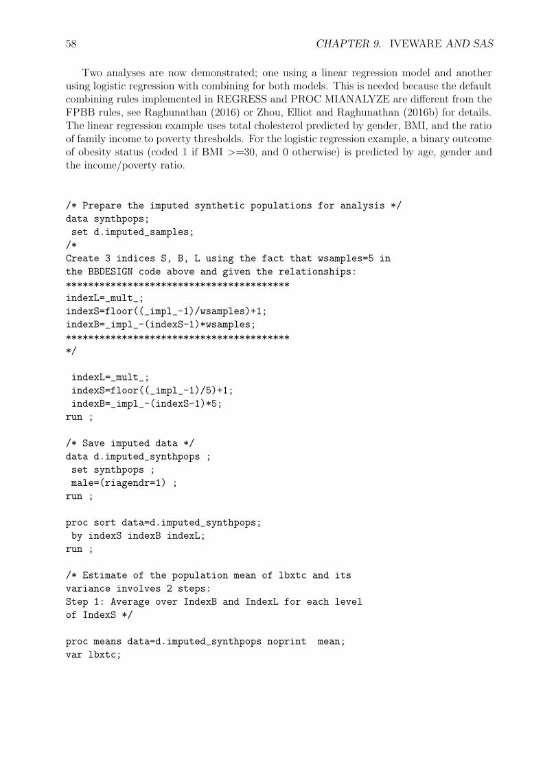
58 CHAPTER 9. IVEWARE AND SAS
Two analyses are now demonstrated; one using a linear regression model and anotherusing logistic regression with combining for both models. This is needed because the defaultcombining rules implemented in REGRESS and PROC MIANALYZE are different from theFPBB rules, see Raghunathan (2016) or Zhou, Elliot and Raghunathan (2016b) for details.The linear regression example uses total cholesterol predicted by gender, BMI, and the ratioof family income to poverty thresholds. For the logistic regression example, a binary outcomeof obesity status (coded 1 if BMI >=30, and 0 otherwise) is predicted by age, gender andthe income/poverty ratio.
/* Prepare the imputed synthetic populations for analysis */
data synthpops;
set d.imputed_samples;
/*
Create 3 indices S, B, L using the fact that wsamples=5 in
the BBDESIGN code above and given the relationships:
****************************************
indexL=_mult_;
indexS=floor((_impl_-1)/wsamples)+1;
indexB=_impl_-(indexS-1)*wsamples;
****************************************
*/
indexL=_mult_;
indexS=floor((_impl_-1)/5)+1;
indexB=_impl_-(indexS-1)*5;
run ;
/* Save imputed data */
data d.imputed_synthpops ;
set synthpops ;
male=(riagendr=1) ;
run ;
proc sort data=d.imputed_synthpops;
by indexS indexB indexL;
run ;
/* Estimate of the population mean of lbxtc and its
variance involves 2 steps:
Step 1: Average over IndexB and IndexL for each level
of IndexS */
proc means data=d.imputed_synthpops noprint mean;
var lbxtc;

9.3. BBDESIGN EXAMPLES 59
by indexS;
output out=step1 mean=lbxtcbar;
run ;
/* Step 2: Compute the mean and variance across the
S synthetic populations */
proc means data=step1 mean var ;
var lbxtcbar;
run ;
/* Linear Regression analysis using PROC REG with
imputed synthetic populations*/
proc reg data=d.imputed_synthpops;
by indexS indexB indexL;
model lbxtc = bmxbmi male indfmpir ;
ods output parameterestimates=outparms ;
run ;
title "Print Out from Linear Regression" ;
proc print data=outparms ;
run ;
/* prepare combined estimates and variance using
two data steps*/
proc means data=outparms mean ;
var estimate ;
where variable =’Intercept’ ;
by indexs ;
output out=step1_0 mean=bobar ;
run ;
proc print data=step1_0 ;
run ;
proc means data=outparms mean ;
var estimate ;
where variable =’BMXBMI’ ;
by indexs ;
output out=step1_1 mean=b1bar ;
run ;
proc print data=step1_1 ;
run ;

60 CHAPTER 9. IVEWARE AND SAS
proc means data=outparms mean ;
var estimate ;
where variable =’male’ ;
by indexs ;
output out=step1_2 mean=b2bar ;
run ;
proc print data=step1_2 ;
run ;
proc means data=outparms mean ;
var estimate ;
where variable =’INDFMPIR’ ;
by indexs ;
output out=step1_3 mean=b3bar ;
run ;
proc print data=step1_3 ;
run ;
* Merge temp data sets into 1 for combining ;
data step1_all ;
merge step1_0 step1_1 step1_2 step1_3 ;
by indexs ;
run ;
proc print data=step1_all ;
run ;
* use merged data above for final step ;
proc means data=step1_all mean var noprint;
var bobar b1bar b2bar b3bar;
output out=step2 mean=intercept bmxbmi male indfmpir
var=vintercept vbmxbmi vmale vindfmpir;
run ;
proc print data=step2 ;
run ;
/* Combine results for parameter estimates from above */
data combine_linear ;
set step2;
df=5-1 ; *Min(S-1,C-H);
tvalue=quantile(’T’,0.975,df);

9.3. BBDESIGN EXAMPLES 61
/* Create arrays for estimate variance se and
lower/upper CI */
array estimate[4] intercept bmxbmi male indfmpir;
array variance[4] vintercept vbmxbmi vmale vindfmpir;
array se[4] se_intercept se_bmxbmi se_male se_indfmpir;
array lower95[4] l95_intercept l95_bmxbmi
l95_male l95_indfmpir;
array upper95[4] u95_intercept u95_bmxbmi
u95_male u95_indfmpir;
do i=1 to 4;
se[i]=sqrt((1+1/5)*variance[i]); * Note that
denominator must match the number used for
"csamples" in the code ;
lower95[i]=estimate[i]-tvalue*se[i];
upper95[i]=estimate[i]+tvalue*se[i];
end;
drop i;
run ;
options nodate nonumber ;
proc print data=combine_linear ;
title "Combined Estimates, SE, Lower and Upper CI from
Linear Regression" ;
var intercept se_intercept l95_intercept
u95_intercept
bmxbmi se_bmxbmi l95_bmxbmi u95_bmxbmi
male se_male l95_male u95_male indfmpir se_indfmpir
l95_indfmpir u95_indfmpir
;
run ;
**********************************************************;
/* Logistic Regression analysis using PROC LOGISTIC,
outcome is obese predicted by male, family income to poverty
and age categories*/
data imputed_synthpops2 ;
set d.imputed_synthpops ;
if bmxbmi >=30 then obese = 1 ; else obese=0 ;
run ;
/*predict probability of being obese by gender and age in
categories and family income to poverty ratio */
proc logistic data=imputed_synthpops2;

62 CHAPTER 9. IVEWARE AND SAS
by indexS indexB indexL;
model obese (event=’1’) = male indfmpir ag3044 ag4559 ag60 ;
ods output parameterestimates=outparms_log ;
run ;
proc print data=outparms_log ;
run ;
/* prepare combined estimates and variance using
two data steps*/
/* Create separate mean by IndexS for each variable */
proc means data=outparms_log mean ;
var estimate ;
where variable =’Intercept’ ;
by indexs ;
output out=step1_0 mean=bobar ;
run ;
proc print data=step1_0 ;
run ;
proc means data=outparms_log mean ;
var estimate ;
where variable =’male’ ;
by indexs ;
output out=step1_1 mean=b1bar ;
run ;
proc print data=step1_1 ;
run ;
proc means data=outparms_log mean ;
var estimate ;
where variable =’INDFMPIR’ ;
by indexs ;
output out=step1_2 mean=b2bar ;
run ;
proc print data=step1_2 ;
run ;
proc means data=outparms_log mean ;
var estimate ;
where variable =’ag3044’ ;
by indexs ;

9.3. BBDESIGN EXAMPLES 63
output out=step1_3 mean=b3bar ;
run ;
proc print data=step1_3 ;
run ;
proc means data=outparms_log mean ;
var estimate ;
where variable =’ag4559’ ;
by indexs ;
output out=step1_4 mean=b4bar ;
run ;
proc print data=step1_4 ;
run ;
proc means data=outparms_log mean ;
var estimate ;
where variable =’ag60’ ;
by indexs ;
output out=step1_5 mean=b5bar ;
run ;
proc print data=step1_5 ;
run ;
data step1_all_log ;
merge step1_0 step1_1 step1_2 step1_3 step1_4 step1_5;
by indexs ;
run ;
proc print data=step1_all_log ;
run ;
/* Prepare combined estimates and variance
using two data steps*/
proc means data=step1_all_log mean var ;
var bobar b1bar b2bar b3bar b4bar b5bar;
output out=step2_log mean=intercept male indfmpir
ag3044 ag4559 ag60
var=vintercept vmale vindfmpir vag3044 vag4559 vag60;
run ;
/* Combine results for logistic regression */
data combine_log ;

64 CHAPTER 9. IVEWARE AND SAS
set step2_log ;
df=5-1 ; *Min(S-1,C-H);
tvalue=quantile(’T’,0.975,df);
/* Create arrays to the calculations */
array estimate[6] intercept male indfmpir ag3044
ag4559 ag60;
array variance[6] vintercept vmale vindfmpir vag3044
vag4559 vag60;
array se[6] se_intercept se_male se_indfmpir
se_ag3044 se_ag4559 se_ag60 ;
array lower95[6] l95_intercept l95_male l95_indfmpir
l95_ag3044 l95_ag4559 l95_ag60;
array upper95[6] u95_intercept u95_male u95_indfmpir
u95_ag3044 u95_ag4559 u95_ag60;
array or[6] or_intercept or_male or_indfmpir
or_ag3044 or_ag4559 or_ag60;
do i=1 to 6;
se[i]=sqrt((1+1/5)*variance[i]);
or[i]=exp(estimate[i]);
lower95[i]=exp(estimate[i]-tvalue*se[i]);
upper95[i]=exp(estimate[i]+tvalue*se[i]);
end;
drop i;
run ;
proc print data=combine_log ;
title "Combined Estimates from Logistic Regression" ;
run ;
</sas>
9.4 DESCRIBE Example
The DESCRIBE example, using NCS-R data, presents a descriptive analysis of age at inter-view and body mass index with a gender contrast. The example uses the 5 imputed data setsfrom IMPUTE along with MI combining rules and design-based variance estimation usingthe default TSL method. Use of the STRATUM, CLUSTER, and WEIGHT statementsdeclare the complex sample design variables and weight to the software. The CONTRASTstatement requests a linear contrast of mean age at interview and Body Mass Index by gen-der. The DESCRIBE command with a mean statement produces a means analysis of age atinterview and BMI. Missing data is excluded, resulting in a complete case analysis.
<sas name="DESCRIBE Example using Imputed Data Sets">

9.5. REGRESS EXAMPLE 65
libname d "P:\IVEware 0.3 documentation 2016\SAS XML Examples";
/* Descriptive Analysis of Age at Interview and BMI, Missing Data Imputed by IVEware */
<describe name="DESCRIBE Example Using Imputed
Data Sets with Design Adjusted Imputed Descriptive Analysis of Age and BMI">
title MI Design-based Description;
datain d.impute_mult1 d.impute_mult2 d.impute_mult3 d.impute_mult4 d.impute_mult5 ;
stratum sestrat;
cluster seclustr;
weight ncsrwtsh ;
model mult;
mean intwage bmi;
contrast sexf;
run;
</describe>
</sas>
9.5 REGRESS Example
The REGRESS example again uses the previously imputed NCS-R data sets as inputs. Thisexample regresses body mass index (BMI) on lifetime Major Depressive Episode, an indicatorof being female, and age at interview. The default variance estimation method in REGRESSis the Jackknife Repeated Replication method. Use of the PLOTS statement will producea number of diagnostic plots with a .png extension. Note that the gnuplot software mustbe included in the ”settings” file (stored in the SRCLIB folder where software installed) forthis to work correctly. One diagnostic plot is included in the selected output given below.
<sas name="REGRESS Example using Imputed Data Sets">
libname d "P:\IVEware 0.3 documentation 2016\SAS XML Examples";
/* Analyze Five Previously Imputed Data Sets using Linear Regression with REGRESS*/
/* Example uses Complex Sample Design Variables and Diagnostic Plots */
<regress name="Linear Regression Example">
title Linear Regression using REGRESS with Imputed Data Sets;
datain d.impute_mult1 d.impute_mult2 d.impute_mult3 d.impute_mult4 d.impute_mult5 ;
estout impute_regress;
stratum sestrat;
cluster seclustr;
weight ncsrwtsh;
dependent bmi;
predictor mde sexf intwage ;
link linear ;
plots outplots ;
run;
</regress>
</sas>
Selected Regression Output
All imputations
Valid cases 9282
Sum weights 9282.000152
Degr freedom 26.42925062
Sum of squares:
Model 3954.942524

66 CHAPTER 9. IVEWARE AND SAS
Error 299501.0663
Total 303456.0088
R-square 0.01303
F-value 0.08725
P-value 0.98565
Variable Estimate Std Error T Test Prob > |T|
Intercept 25.9222187 0.2549001 101.69559 0.00000
mde 0.8287332 0.1234398 6.71366 0.00000
sexf -0.6898597 0.1395496 -4.94347 0.00004
intwage 0.0290391 0.0049550 5.86059 0.00000
Variable Estimate 95% Confidence Interval
Lower Upper
Intercept 25.9222187 25.3986774 26.4457600
mde 0.8287332 0.5751993 1.0822672
sexf -0.6898597 -0.9764816 -0.4032378
intwage 0.0290391 0.0188620 0.0392162
Variable Design SRS % Diff
Effect Estimate SRS v Est
Intercept 1.48293 26.3002986 1.45852
mde 0.60113 0.8344926 0.69496
sexf 1.17056 -0.6735030 -2.37102
intwage 1.58580 0.0231927 -20.13297
9.6 SASMOD Example
The SASMOD command is available with IVEware and SAS only. This command is basedupon the Jackknife Repeated Replication method for variance estimation and can be usedwith many SAS procedures (see previous sections of this chapter). In this example, PROCCATMOD is used to execute an MI and design-based log-linear model. The model examinesrelationships between gender and Major Depressive Episode, using the 5 previously imputed

9.7. SYNTHESIZE EXAMPLES 67
NCS-R data sets as input.
<sas name="SASMOD with PROC CATMOD">
libname d ’P:\IVEware 0.3 documentation 2016\SAS XML Examples’;
/* Analyze 5 Imputed Data Sets with JRR Variance Estimation PROC CATMOD for Log-Linear Model */
<sasmod name="SASMOD for Log-Linear Model with PROC CATMOD">
title SASMOD Example ;
datain d.impute_mult1 d.impute_mult2 d.impute_mult3 d.impute_mult4 d.impute_mult5 ;
estout modexam;
cluster seclustr ;
stratum sestrat ;
weight ncsrwtsh;
/* SAS statements begin here */
proc catmod;
model mde*sexf =_response_ / pred=freq;
loglin mde sexf mde*sexf ;
run;
</sasmod>
</sas>
Selected Output
All imputations
Valid cases 9282
Sum weights 9282.000152
Degr freedom Infinite
-2 LogLike 21833.80757
Variable Estimate Std Error Wald test Prob > Chi
mde 0 0.7346635 0.0173232 1798.53648 0.00000
sexf 0 -0.1223741 0.0115333 112.58311 0.00000
mde*sexf 0 0 0.1283257 0.0168590 57.93785 0.00000
Variable Estimate 95% Confidence Interval
Lower Upper
mde 0 0.7346635 0.7006693 0.7686577
sexf 0 -0.1223741 -0.1450064 -0.0997418
mde*sexf 0 0 0.1283257 0.0952424 0.1614090
9.7 SYNTHESIZE Examples
9.7.1 Fully Synthesized Data Set
The first SYNTHESIZE example demonstrates multiple imputation of missing data followedby synthesis of each variable in the Primary Cardiac Arrest data set. In the code below,we request 5 multiple imputations with 5 implicates or synthesized data sets per imputationmultiple. Use of similar syntax as from IMPUTE is utilized along with the SYNTHESIZEstatement to declare the variables to be synthesized. The imputation is done before thesynthesis, therefore each of 5 imputation multiples contains 5 synthesized data sets for sub-sequent analysis. Two key variables are created during this process: IMPL with values of1,2,3,4,5 denoting synthesized data sets 1-5, and MULT with values of 1,2,3,4,5 denotingimputations. The final part of this example demonstrates correct combining rules for fullysynthesized and imputed data (Raghunathan (2015), page 168).

68 CHAPTER 9. IVEWARE AND SAS
/* Synthesize Example Using PCA and Omega 3 Fatty Acids Data */
<sas name="SYNTHESIZE Example">
/* Set libnames */
libname d1 ’P:\IVEware_and_MI_Applications_Book\DataSets\PCA and Omega 3 Fatty Acids Data’ ;
libname dout ’P:\IVEware 0.3 documentation 2016\SAS XML Examples’;
<synthesize name="Synthesize All Variables Using PCA and Omega3 Data">
datain d1.test;
continuous AGE NUMCIG YRSSMOKE FATINDEX DHA_EPA REDTOT WGTKG TOTLKCAL HGTCM ;
categorical CASECNT GENDER RACE3 HYPER DIAB SMOKE FAMMI EDUSUBJ3 CHOLESTH ;
mixed CAFFTOT ALCOHOL3 ;
transfer STUDYID ;
synthesize CASECNT AGE GENDER RACE3 HYPER DIAB SMOKE NUMCIG YRSSMOKE FATINDEX
FAMMI EDUSUBJ3 DHA_EPA REDTOT CHOLESTH CAFFTOT WGTKG TOTLKCAL ALCOHOL3 HGTCM ;
restrict NUMCIG(smoke=2,3) YRSSMOKE(smoke=2,3) ;
bounds NUMCIG(>0) YRSSMOKE(>0, <age-12) DHA_EPA(>0) REDTOT(>0)
CAFFTOT(>0) TOTLKCAL(>0) ALCOHOL3(>0);
ITERATIONS 2;
MULTIPLES 5;
SEED 2001;
IMPLICATES 5;
DATAOUT dout.synthesize all ;
run;
</synthesize>
/* Examine Contents of Output Data Set*/
proc contents data=dout.synthesize ;
run ;
data synthesized ;
set dout.synthesize ;
* use implicates 1-5 only ;
if _impl_ >=1 then _imputation_= cat(_mult_, _impl_) ;
run ;
proc freq ;
tables _mult_*_impl_ _imputation_ ;
run ;
proc sort data=synthesized ;
by _imputation_ ;
run ;
/* Obtain mean kcalories per day by _imputation_ and then combine using correct rules for synthesized data*/
proc means data=synthesized (where=(_imputation_ ne ’ ’ )) mean stderr ;
var totlkcal ;
by _imputation_ ;
ods output summary=outstat ;
run ;
proc print data=outstat ;
run ;
proc sql ;
create table outstat1
as select *, mean(totlkcal_mean) as qbar, mean(totlkcal_stderr*totlkcal_stderr) as ubar
from outstat ;
proc sql ;
create table outstat2
as select *, sum((totlkcal_mean - qbar)**2)/24 as btwvar
from outstat1
/* Combining rules for fully imputed and synthesized data*/
data final ;
set outstat2 ;
if _n_=1 ;
syn_estimate=qbar ;

9.7. SYNTHESIZE EXAMPLES 69
syn_variance=ubar ;
syn_se=sqrt(syn_variance) ;
btw=btwvar ;
total_syn_var=((1+1/25)*btwvar) - ubar ;
proc print data=final ;
var syn_estimate syn_se syn_variance btwvar total_syn_var;
run ;
Results from Fully Synthesized Data SetParameter Mean SE Total Variance
Total Kilocalories 1822.24 40.44 106.10
9.7.2 Partially Synthesized Data Set
The second SYNTHESIZE example demonstrates how to synthesize just selected ”sensitive”variables, again using the PCA data set. As a reminder, multiple imputation is done beforesynthesis, therefore each of 3 imputation multiples contains 5 synthesized data sets. Twokey variables are created during this process: IMPL with values of 1,2,3,4,5 denoting im-plicates and MULT with values of 1,2,3 denoting imputations. The syntax below includesimputation and synthesis followed by an example of application of correct combining rulesfor partially synthesized data (Raghunathan, (2015) page 168).
/* Partial Synthesize Example Using PCA and Omega 3 Fatty Acids Data */
<sas name="SYNTHESIZE Partial Example">
/* Set libnames */
libname d1 ’P:\IVEware_and_MI_Applications_Book\DataSets\PCA and Omega 3 Fatty Acids Data’ ;
libname dout ’P:\IVEware 0.3 documentation 2016\SAS XML Examples’;
<synthesize name="Synthesize Selected Variables Using PCA and Omega3 Data">
datain d1.test;
continuous AGE NUMCIG YRSSMOKE FATINDEX DHA_EPA REDTOT WGTKG TOTLKCAL HGTCM ;
categorical CASECNT GENDER RACE3 HYPER DIAB SMOKE FAMMI EDUSUBJ3 CHOLESTH ;
mixed CAFFTOT ALCOHOL3 ;
transfer STUDYID ;
/* synthesize select health and personal information variables */
synthesize CASECNT HYPER DIAB FATINDEX FAMMI DHA_EPA REDTOT WGTKG HGTCM ;
restrict NUMCIG(smoke=2,3) YRSSMOKE(smoke=2,3) ;
bounds NUMCIG(>0) YRSSMOKE(>0, <age-12) DHA_EPA(>0) REDTOT(>0) CAFFTOT(>0) TOTLKCAL(>0) ALCOHOL3(>0);
ITERATIONS 2;
MULTIPLES 3;
SEED 2001;
IMPLICATES 5;
DATAOUT dout.synthesize_partial all ;
run;
</synthesize>
proc sort data=dout.synthesize_partial ;
by _mult_ _impl_ ;
run ;
data synthesized ;
set dout.synthesize_partial ;
* use implicates 1-5 only ;
if _impl_ >=1 then _imputation_= cat(_mult_, _impl_) ;
run ;

70 CHAPTER 9. IVEWARE AND SAS
proc freq ;
tables _mult_*_impl_ _imputation_ ;
run ;
proc sort data=synthesized ;
by _imputation_ ;
run ;
/* Obtain mean fatindex by _imputation_ and then combine using correct rules for synthesized data*/
proc means data=synthesized (where=(_imputation_ ne ’ ’ )) mean stderr ;
var fatindex ;
by _imputation_ ;
ods output summary=outstat ;
run ;
proc print data=outstat ;
run ;
proc sql ;
create table outstat1
as select *, mean(fatindex_mean) as qbar, mean(fatindex_stderr*fatindex_stderr) as ubar
from outstat ;
proc sql ;
create table outstat2
as select *, sum((fatindex_mean - qbar)**2) as sumdiffs, calculated sumdiffs/14 as btwvar
from outstat1 ;
/* Combining rules for fully imputed and partially synthesized data are different from fully synthesized data*/
data final ;
set outstat2 ;
if _n_=1 ;
syn_estimate=qbar ;
syn_variance=ubar ;
syn_se=sqrt(syn_variance) ;
/* total variance is ubar + btwvar/m */
total_partialsyn_var=ubar + btwvar/15 ;
proc print data=final ;
var syn_estimate syn_se syn_variance btwvar total_partialsyn_var;
run ;
</sas>
Results from Partially Synthesized and Imputed Data SetsParameter Mean SE Total VarianceFatIndex 21.56 0.14 0.02
9.8 COMBINE Example
The COMBINE example joins four waves of Health and Retirement Survey data from 2006,2008, 2010 and 2012. Though the data sets have the same variable names and values, eachhas manufactured missing data on some variables. For example, the HRS 2006 data hasno observed data on three variables: DIABETES, ARTHRITIS, and SELFRHEALTH, HRS2008 data is completely missing on DIABETES and ARTHRITIS but has observed data onSELFRHEALTH, and so on. In addition, other variables such as marital status (MARCAT)have small amounts of missing data in some or all waves of data. This example demonstratesa three step process: 1. ”stacking” the data using COMBINE, 2. imputing the missing datain the combined data set using IMPUTE, and 3. use of DESCRIBE to perform MI and

9.8. COMBINE EXAMPLE 71
design-based descriptive analysis of arthritis by year.
<sas name="COMBINE Example using 4 Waves of HRS Data">
libname d "P:\IVEware_and_MI_Applications_Book\Chapter2DataSources";
/* COMBINE Example Using HRS 2006 2008 2010 and 2012 Data */
<combine name="COMBINE Example">
datain d.hrs2006_27jul2016 d.hrs2008_27jul2016 d.hrs2010_27jul2016 d.hrs2012_27jul2016 ;
dataout d.combined_hrs_2006_2012 ;
run;
</combine>
/* Use SAS to Examine Contents of Combined Data */
proc contents data=d.combined_hrs_2006_2012 ;
run ;
/* Examine Means of Combined Data */
proc means n nmiss mean min max data=d.combined_hrs_2006_2012 ;
class yr ;
run ;
/* Use IMPUTE to impute missing data */
<impute name="Impute_Post_COMBINE">
datain d.combined_hrs_2006_2012 ;
dataout d.impute_mult1;
default categorical;
continuous stratum age wgt;
transfer hhid pn ;
iterations 5;
multiples 5;
seed 2016 ;
run;
</impute>
/* Extract remaining 4 data sets */
<putdata name="Impute_Post_combine" mult="2" dataout="d.impute_mult2" />
<putdata name="Impute_Post_combine" mult="3" dataout="d.impute_mult3" />
<putdata name="Impute_Post_combine" mult="4" dataout="d.impute_mult4" />
<putdata name="Impute_Post_combine" mult="5" dataout="d.impute_mult5" />
/* Use Imputed Data Sets for Descriptive Analysis*/
<describe name="Descriptive Analysis of Combined and Imputed Arthritis by Year">
datain d.impute_mult1 d.impute_mult2 d.impute_mult3 d.impute_mult4 d.impute_mult5 ;
stratum stratum ;
cluster secu;
weight wgt ;
table arthritis ;
by yr ;
run;
</describe>
</sas>
Proportion of Arthritis by Year, Based on Combined, Imputed HRS DataOutcome Year Mean SE
Diagnosis of Arthritis 2006 0.548 0.007” 2008 0.567 0.008” 2010 0.532 0.006” 2012 0.550 0.008

Chapter 10
IVEware and Stata, SPSS, and R
10.1 Introduction
Chapter 10 presents syntax to replicate the examples in Chapter 9, again using IVEwarewith the SRCware Shell editor with Stata, SPSS and R. In this chapter, just the IVEwarecommand syntax is presented while subsequent coding and analyses are left to the analystto code in a software of choice. Though the software with IVEware differs, the IVEwaresyntax and resultant output should match the Chapter 9 examples.
10.2 IMPUTE Example, IVEware and Stata
The first example demonstrates use of IVEware and Stata with IMPUTE, using NCS-Rdata. After imputation, the 5 multiples are stored in data sets called ”impute mult1-impute mult5”. By default, these are saved in Stata .dta format and can be used in additionalanalyses.
<stata name="Impute Example with Stata">
use "P:\IVEware_and_MI_Applications_Book\Chapter3\Examples\Stata\ncsr_ex1.dta"
/* Multiple Imputation*/
<impute name="Impute">
title Multiple Imputation Using IMPUTE ;
datain ncsr_ex1 ;
dataout impute_mult1;
default categorical;
continuous bmi intwage ncsrwtsh sestrat;
transfer caseid;
iterations 5;
multiples 5;
seed 2001;
run;
</impute>
/*Extract remaining 4 data sets*/
<putdata name="Impute" mult="2" dataout="impute_mult2"/>
<putdata name="Impute" mult="3" dataout="impute_mult3"/>
<putdata name="Impute" mult="4" dataout="impute_mult4"/>
<putdata name="Impute" mult="5" dataout="impute_mult5"/>
</stata>
72

10.3. BBDESIGN EXAMPLE, IVEWARE AND SPSS 73
10.3 BBDESIGN Example, IVEware and SPSS
Section 10.3 demonstrates use of IVEware and SPSS with the BBDESIGN command toproduce an output population data set called ”bbdesign samples.sav” (SPSS format). Asusual, the output data set can be used in additional analyses within SPSS or transferred toanother statistical software package.
<spss name="BBDESIGN Examples">
/* example uses 2011 - 2012 NHANES data, subset for age 18+ for adults*/
/* SPSS .sav file is stored in working folder */
<bbdesign name="BBdesign">
title Use of BBdesign;
datain nhanes1112_adult;
dataout bbdesign_samples ;
stratum sdmvstra ;
cluster sdmvpsu ;
weight wtmec2yr ;
csamples 5 ;
wsamples 5 ;
seed 2001;
run;
</bbdesign>
</spss>
10.4 DESCRIBE Example, IVEware and R
The DESCRIBE command uses IVEware and R to perform a descriptive analysis of age ofinterview and Body Mass Index with a gender contrast. This examples uses NCS-R datawith a design-based/multiple imputation approach for variance estimation. The five previ-ously imputed NCS-R data sets are first imported into R and then used in the DESCRIBEcommand.
<R name="DESCRIBE Example">
# iveware examples - R version
# import the input datasets
impute_mult1 <- read.delim("impute_mult1.txt")
save(impute_mult1, file="impute_mult1.rda")
impute_mult2 <- read.delim("impute_mult2.txt")
save(impute_mult2, file="impute_mult2.rda")
impute_mult3 <- read.delim("impute_mult3.txt")
save(impute_mult3, file="impute_mult3.rda")
impute_mult4 <- read.delim("impute_mult4.txt")
save(impute_mult4, file="impute_mult4.rda")
impute_mult5 <- read.delim("impute_mult5.txt")
save(impute_mult5, file="impute_mult5.rda")
# Descriptive Analysis of Age at Interview and BMI
<describe name="DESCRIBE">
title MI Design-based Description;
datain impute_mult1 impute_mult2 impute_mult3 impute_mult4 impute_mult5;
stratum sestrat;
cluster seclustr;
weight ncsrwtsh ;
model mult;
mean intwage bmi;

74 CHAPTER 10. IVEWARE AND STATA, SPSS, AND R
contrast sexf;
run;
</describe>
</R>
10.5 REGRESS Example, IVEware and StataThe REGRESS example inputs five previously imputed NCS-R data sets and performs linearregression with IVEware and Stata. Note that the imputed input data sets were previouslystored as Stata data sets in .dta format.
<stata name="REGRESS Example with Stata">
/* Analyze 5 imputed data sets with Linear Regression */
<regress name="REGRESS for Linear Regression with Imputed Data Sets">
title Example of REGRESS ;
datain impute_mult1 impute_mult2 impute_mult3 impute_mult4 impute_mult5 ;
estout impute_regress;
stratum sestrat;
cluster seclustr;
weight ncsrwtsh;
dependent bmi;
predictor mde sexf intwage ;
run;
</regress>
</stata>
10.6 SYNTHESIZE Example, IVEware and Stata
This example uses IVEware and Stata to synthesize all variables in the Primary CardiacArrest data set. An output data set called ”synthesize.dta” contains the synthesized andmultiply imputed data.
* Synthesize Example Using PCA and Omega 3 Fatty Acids Data */
<stata name="SYNTHESIZE Example">
<synthesize name="Synthesize All Variables Using PCA and Omega3 Data">
datain test;
continuous AGE NUMCIG YRSSMOKE FATINDEX DHA_EPA REDTOT WGTKG TOTLKCAL HGTCM ;
categorical CASECNT GENDER RACE3 HYPER DIAB SMOKE FAMMI EDUSUBJ3 CHOLESTH ;
mixed CAFFTOT ALCOHOL3 ;
transfer STUDYID ;
synthesize CASECNT AGE GENDER RACE3 HYPER DIAB SMOKE NUMCIG YRSSMOKE FATINDEX
FAMMI EDUSUBJ3 DHA_EPA REDTOT CHOLESTH CAFFTOT WGTKG TOTLKCAL ALCOHOL3 HGTCM ;
restrict NUMCIG(smoke=2,3) YRSSMOKE(smoke=2,3) ;
bounds NUMCIG(>0) YRSSMOKE(>0, <age-12) DHA_EPA(>0) REDTOT(>0) CAFFTOT(>0) TOTLKCAL(>0) ALCOHOL3(>0);
ITERATIONS 2;
MULTIPLES 5;
SEED 2001;
IMPLICATES 5;
DATAOUT synthesize all ;
run;
</synthesize>
</stata>
10.7 COMBINE Example, IVEware and R
The COMBINE example pairs IVEware with R to demonstrate how to combine multipledata sets. The four HRS data sets (2006, 2008, 2010, 2012) are first imported into R

10.7. COMBINE EXAMPLE, IVEWARE AND R 75
using the Foreign package and then concatenated by COMBINE. An output data set called”combined hrs 2006 2012” in R format is created for subsequent imputation and analysis.
<R name="COMBINE Example">
# iveware examples - R version
# load foreign package and read in SAS data sets
library(foreign)
hrs2006_27jul2016r <- read.xport("hrs2006_27jul2016.xpt")
hrs2008_27jul2016r <- read.xport("hrs2008_27jul2016.xpt")
hrs2010_27jul2016r <- read.xport("hrs2010_27jul2016.xpt")
hrs2012_27jul2016r <- read.xport("hrs2012_27jul2016.xpt")
<combine name="COMBINE_Example_R">
datain hrs2006_27jul2016r hrs2008_27jul2016r hrs2010_27jul2016r hrs2012_27jul2016r ;
dataout combined_hrs_2006_2012;
run;
</combine>
summary(combined_hrs_2006_2012)
</R>

Chapter 11
SRCWare
11.1 Introduction
Chapter 11 demonstrates use of SRCWare, the stand-alone version of IVEware. This chapterincludes examples of the IMPUTE, BBDESIGN, DESCRIBE, REGRESS, SYNTHESIZE,and COMBINE commands. Input data sets are read into SRCWare using the GETDATAcommand while data sets from SRCWare can be output using the PUTDATA command.Output data sets can be used in subsequent analyses using a software of choice. For examplesof the GETDATA and PUTDATA commands, see Section 1.6 and provided examples on theIVEware website. Because the IVEware commands have been detailed in previous chapters,just the code is presented in this chapter.
11.2 IMPUTE Example<srcware name="SRCWARE_IMPUTE">
/* import the input datasets */
<getdata name="ncsr_ex1">
table ncsr_ex1.txt;
run;
</getdata>
/* Multiple Imputation using IMPUTE*/
<impute name="MI">
title Multiple Imputation Using IMPUTE ;
datain ncsr_ex1 ;
dataout impute_mult1;
default categorical;
continuous bmi intwage ncsrwtsh sestrat ;
transfer caseid ;
iterations 5;
multiples 5;
seed 2001;
run;
</impute>
/* Extract remaining data sets */
<putdata name="MI" mult="2" dataout="impute_mult2" />
<putdata name="MI" mult="3" dataout="impute_mult3" />
<putdata name="MI" mult="4" dataout="impute_mult4" />
<putdata name="MI" mult="5" dataout="impute_mult5" />
76

11.3. BBDESIGN EXAMPLE 77
</srcware>
11.3 BBDESIGN Example<srcware name="SRCWARE_BBDESIGN">
/* import the input dataset*/
<getdata name="nhanes1112_adult">
table nhanes1112_adult.txt;
run;
</getdata>
<bbdesign name="BBdesign">
title Use of BBdesign;
datain nhanes1112_adult;
dataout bbdesign_samples ;
stratum sdmvstra ;
cluster sdmvpsu ;
weight wtmec2yr ;
csamples 5 ;
wsamples 5 ;
seed 2001;
run;
</bbdesign>
</srcware>
11.4 DESCRIBE Example<srcware name="SRCWARE_IMPUTE">
/* import the input dataset */
<getdata name="ncsr_ex1">
table ncsr_ex1.txt;
run;
</getdata>
/* Review of Multiple Imputation using IMPUTE*/
<impute name="MI">
title Multiple Imputation Using IMPUTE ;
datain ncsr_ex1 ;
dataout impute_mult1;
default categorical;
continuous bmi intwage ncsrwtsh sestrat ;
transfer caseid ;
iterations 5;
multiples 5;
seed 2001;
run;
</impute>
/* Extract remaining data sets */
<putdata name="MI" mult="2" dataout="impute_mult2" />
<putdata name="MI" mult="3" dataout="impute_mult3" />
<putdata name="MI" mult="4" dataout="impute_mult4" />
<putdata name="MI" mult="5" dataout="impute_mult5" />
/* Descriptive Analysis of Age at Interview and BMI, Missing Data Imputed by IVEware */
<describe name="DESCRIBE">
title MI Design-based Description;
datain impute_mult1 impute_mult2 impute_mult3 impute_mult4 impute_mult5 ;
stratum sestrat;
cluster seclustr;

78 CHAPTER 11. SRCWARE
weight ncsrwtsh ;
model mult;
mean intwage bmi;
contrast sexf;
run;
</describe>
</scrware>
11.5 REGRESS Example<srcware name="SRCWARE_IMPUTE">
/* import the input datasets */
<getdata name="ncsr_ex1">
table ncsr_ex1.txt;
run;
</getdata>
/* Review of Multiple Imputation using IMPUTE*/
<impute name="MI">
title Multiple Imputation Using IMPUTE ;
datain ncsr_ex1 ;
dataout impute_mult1;
default categorical;
continuous bmi intwage ncsrwtsh sestrat ;
transfer caseid ;
iterations 5;
multiples 5;
seed 2001;
run;
</impute>
/* Extract remaining data sets */
<putdata name="MI" mult="2" dataout="impute_mult2" />
<putdata name="MI" mult="3" dataout="impute_mult3" />
<putdata name="MI" mult="4" dataout="impute_mult4" />
<putdata name="MI" mult="5" dataout="impute_mult5" />
/* Analyze Previously Imputed Data Sets using Linear Regression with REGRESS */
/* Example uses Complex Sample Design Variables and Weight Plus Plots */
<regress name="REGRESS">
title Linear Regression using REGRESS with Imputed Data Sets;
datain impute_mult1 impute_mult2 impute_mult3 impute_mult4 impute_mult5 ;
estout impute_regress;
stratum sestrat;
cluster seclustr;
weight ncsrwtsh;
dependent bmi;
predictor mde sexf intwage ;
link linear ;
plots outplots ;
run;
</regress>
</srcware>
11.6 SYNTHESIZE Example<srcware name="SRCWARE_SYNTHESIZE">
/* import the input datasets */
<getdata name="test">
table test.txt;
run;
</getdata>

11.7. COMBINE EXAMPLE 79
/* Use SYNTHESIZE command to prepare fully synthesized data set*/
<synthesize name="Synthesize">
datain test;
continuous AGE NUMCIG YRSSMOKE FATINDEX DHA_EPA REDTOT WGTKG TOTLKCAL HGTCM ;
categorical CASECNT GENDER RACE3 HYPER DIAB SMOKE FAMMI EDUSUBJ3 CHOLESTH ;
mixed CAFFTOT ALCOHOL3 ;
transfer STUDYID ;
synthesize CASECNT AGE GENDER RACE3 HYPER DIAB SMOKE NUMCIG
YRSSMOKE FATINDEX FAMMI EDUSUBJ3 DHA_EPA REDTOT CHOLESTH CAFFTOT WGTKG TOTLKCAL
ALCOHOL3 HGTCM ;
restrict NUMCIG(smoke=2,3) YRSSMOKE(smoke=2,3) ;
bounds NUMCIG(>0) YRSSMOKE(>0, <age-12) DHA_EPA(>0) REDTOT(>0) CAFFTOT(>0) TOTLKCAL(>0) ALCOHOL3(>0);
ITERATIONS 2;
MULTIPLES 5;
SEED 2001;
IMPLICATES 5;
DATAOUT synthesize all ;
run;
</synthesize>
</srcware>
11.7 COMBINE Example<srcware name="SRCWARE_COMBINE">
/* import the input datasets */
<getdata name="hrs2006_27jul2016">
table hrs2006_27jul2016.csv;
run;
</getdata>
<getdata name="hrs2008_27jul2016">
table hrs2008_27jul2016.csv;
run;
</getdata>
<getdata name="hrs2010_27jul2016">
table hrs2010_27jul2016.csv;
run;
</getdata>
<getdata name="hrs2012_27jul2016">
table hrs2012_27jul2016.csv;
run;
</getdata>
/* COMBINE Example Using HRS 2006 2008 2010 and 2012 Data*/
<combine name="COMBINE">
datain hrs2006_27jul2016 hrs2008_27jul2016 hrs2010_27jul2016 hrs2012_27jul2016 ;
dataout combined_hrs_2006_2012 all ;
run;
</combine>
</srcware>

Bibliography
[1] Atkinson, A. C. (1987). Plots, transformations and regression: An introduction to graphical methods of diagnostic regres-sion analysis. Journal of the Royal Statistical Society.Series A (General), 150(2)
[2] Bondarenko, I. & Raghunathan, T. E. (2010). Multiple imputation for causal inference. Arbor, 1001(48109)
[3] Bondarenko, I. & Raghunathan, T. E. (2016). Graphical and numerical diagnostic tools to assess suitability of multipleimputations and imputation models. Statistics in Medicine, 35, 3007-3020.
[4] Dong, Q., Elliott, M. R. & Raghunathan, T. E. (2014a). A nonparametric method to generate synthetic populations toadjust for complex sampling design features. Survey Methodology, 40(1), 29-46.
[5] Dong, Q., Elliott, M. R. & Raghunathan, T. E. (2014b). Combining information from multiple complex surveys. SurveyMethodology, 40, 347-354.
[6] Gelman, A., Carlin, J. B., Stern, H. S. & Rubin, D. B. (1995). Bayesian data analysis. London: Chapman and Hall.
[7] Gelman, A. & Hill, J. (2006). Data analysis using regression and Multilevel/Hierarchical models. New York: CambridgeUniversity Press.
[8] He, Y. & Raghunathan, T. E. (2006). Tukey’s gh distribution for multiple imputation. The American Statistician, 60,251-256: Response.
[9] Heeringa, S. G., Little, R. J. A., & Raghunathan, T. E. (1997). Imputation of multivariate data on household net worth.University of Michigan, Ann Arbor, Michigan,
[10] Kish, L. & Frankel, M. (1974). Inference from complex systems. Journal of the Royal Statistical Society.Series B (Method-ological), 36(1), 1-37.
[11] Li, K. H., Raghunathan, T. E. & Rubin, D. B. (1991). Large-sample significance levels from multiply imputed datausing moment-based statistics and an F-reference distribution. Journal of the American Statistical Association, 86(416),1065-1073.
[12] Raghunathan, T. E. (1994). Monte carlo methods for exploring sensitivity to distributional assumptions in a bayesiananalysis of a series of 2 2 tables. Statistics in Medicine, 13(15), 1525-1538.
[13] Raghunathan, T. E., Lepkowski, J. M., Hoewyk, J. V. & Solenberger, P. (2001). A multivariate technique for multiplyimputing missing values using a sequence of regression models. Survey Methodology, 27(1), 85-95.
[14] Raghunathan, T. E., Reiter, J. P. & Rubin, D. B. (2003). Multiple imputation for statistical disclosure limitation. Journalof Official Statistics-Stockholm-, 19(1), 1-16.
[15] Raghunathan, T. E. & Rubin, D. B. (1998). Roles for Bayesian techniques in survey sampling. Proceedings of the SilverJubilee Meeting of the Statistical Society of Canada, , 51-55.
[16] Raghunathan, T. E. (2015). In Chapman & Hall/CRC Interdisciplinary Statistics Series (Ed.), Missing data analysis inpractice. Boca Raton: CRC Press.
[17] Raghunathan, T. E, Berglund, P., and Solenberger, P. W. (2017). Multiple Imputation in Practice: With Examples UsingIVEware. Boca Raton: CRC Press (Forthcoming).
[18] Reiter, J. (2002). Satisfying disclosure restrictions with synthetic data sets. Journal of Official Statistics, 18(4), 531-543.
[19] Rubin, D. B. (1976). Inference and missing data. Biometrika, 63(3), 581-592.
80

BIBLIOGRAPHY 81
[20] Rubin, D. B. (1987b). Multiple imputation for nonresponse in surveys (99th ed.) Wiley.
[21] Schenker, N., Raghunathan, T. E. & Bondarenko, I. (2010). Improving on analyses of self-reported data in a large-scalehealth survey by using information from an examination-based survey. Statistics in Medicine, 29(5), 533-545.
[22] van Buuren, S. (2012). Flexible imputation of missing data. Chapman and Hall/CRC.
[23] van Buuren, S. & Oudshoorn, K. (1999). Flexible multivariate imputation by MICE. Technical Report, Leiden: TNOPreventie En Gezondheid, TNO/VGZ/PG 99.054.
[24] Vittinghoff, E., Glidden, D. V., Shiboski, S. C. & McCulloch, C. E. (2005). Regression methods in biostatistics: Linear,logistic, survival, and repeated measures models. New York, NY, US: Springer Publishing Co.
[25] Weisberg, S. (2013). Applied linear regression (4th ed.) Wiley.
[26] Zhou, H., Elliott, M. R. & Raghunathan, T. E. (2016). Synthetic Multiple-Imputation Procedure for Multistage ComplexSamples, Journal of Official Statistics, 32, 231-256.
[27] Zhou, H., Elliott, M. R.& Raghunathan, T. E. (2016). Multiple imputation in two-stage cluster samples using the weightedfinite population bayesian bootstrap. Journal of Survey Statistics and Methodology, 4, 139-170.
[28] Zhou, H., Elliott, M. R. & Raghunathan, T. E. (2015). A two-step semiparametric method to accommodate samplingweights in multiple imputation. Biometrics, 72, 242-252.