iVAMS 2.0: Machine-Learning-Metamodel-Integrated IntelligentVerilog-AMS for Fast and Accurate Mixed-Signal Design

Optimization

July 3, 2019

Saraju P. Mohanty Elias KougianosComputer Science and Engineering Engineering Technology

University of North Texas, Denton, TX 76203. University of North Texas, Denton, TX 76203.Email: saraju.mohanty@unt.edu Email: elias.kougianos@unt.edu

Abstract

The gap between abstraction levels in analog design is a major obstacle for advancing analog andmixed-signal (AMS) design automation and computer-aided design (CAD). Intelligent models for low-level analog building blocks are needed to bridge the accuracy gap between behavioral and transistor-level simulations. The models should be able to accurately estimate the characteristics of the analogblock over a large design space. Machine learning (ML) models based on actual silicon have thecapabilities of capturing detailed characteristics of complex designs. In this paper, a ML model calledArtificial Neural Network Metamodels (ANNM) have been explored to capture the highly nonlinearnature of analog blocks. The application of these intelligent models to multi-objective analog blockoptimization is demonstrated. Parameterized behavioral models in Verilog-AMS based on the artificialneural network metamodels are constructed for efficient system-level design exploration. To the best ofthe authors’ knowledge this is the first paper to integrate artificial neural network models in Verilog-AMS, which is called iVAMS 2.0. To demonstrate the application of iVAMS 2.0, this paper presentstwo case studies: an operational amplifier (OP-AMP) and a phase-locked loop (PLL). A biologically-inspired “firefly optimization algorithm” is applied to an OP-AMP design in the iVAMS 2.0 framework.The optimization process is sped up by 5580× due to the use of iVAMS with negligible loss in accuracy.Similarly, for a PLL design, the physical design aware ANNs are trained and used as metamodels topredict its frequency, locking time, and power. Thorough experimental results demonstrate that only100 sample points are sufficient for ANNs to predict the output of circuits with 21 design parameterswithin 3% accuracy, which improves the accuracy by 56% as compared to polynomial metamodels. Aproposed artificial bee colony (ABC) based algorithm performs optimization over the ANN metamodelsof the PLL. It is observed that the ANN metamodels achieve more accurate results than polynomialmetamodels with shorter optimization time.

Keywords— Machine Learning Models, Artificial Neural Networks (ANN), Intelligent Verilog-AMS,Metamodeling, System Simulation, Mixed-Signal Design, Behavioral Simulation, Verilog-AMS Modeling,OP-AMP, Phase-Locked Loop (PLL)

1 Introduction

Competitive time-to-market and design constraints discourage or prohibit the use of slow exhaustive designspace exploration to reach fully optimal performance for complex nano-CMOS mixed-signal designs. The

1

arX

iv:1

907.

0152

6v1

[ee

ss.S

P] 1

1 Ju

n 20

19

trend of integrated circuit (IC) development toward increasing levels of integration has never stopped.Design automation tools and flows for digital IC systems have followed this trend due to the fact thatdigital circuits have higher regularity and high margin for noise and process variations [1, 2]. Thus theirperformance can be well controlled throughout different abstraction levels from top to bottom. In contrast,a hierarchical way to tightly control and predict the performance of analog and mixed-signal (AMS) blocksat every design phase has not yet been established in industrial practice.

Modern AMS systems are complex and contain numerous nanometer devices. In order to achieve highperformance and high yield, a system must be optimized at both system and circuit levels [3, 4, 5]. For a top-down design approach, this process starts with designing and optimizing the system with sub-block modelsat high levels of abstraction. The specifications for each sub-block that lead to the best system performanceare then obtained. Each sub-block is then designed and optimized toward these specifications. The issuewith this approach is that generating a perfect model, if it is even possible, takes significant effort. Thereforesome characteristics of the sub-blocks are ignored at the high level simulation. This makes the obtainedsub-block specification compliance less reliable. In other words, optimizing the sub-blocks using thesespecifications does not guarantee satisfying system performance [6]. Usually numerous design iterationsare required. To make the problem worse, performing time-domain simulations (transient analyses) is animportant step when evaluating an AMS system and this process consumes large amount of computationaltime. The parasitics of the physical design of the sub-blocks further aggravate this problem considering thefact that redoing the layout manually may be necessary.

This work proposes developing a design and optimization methodology that not only can generatecompliant designs but can also complete the whole process in much shorter time, compared to conventionalapproaches. Fig. 1 illustrates the potential benefit of using a metamodel-assisted optimization flow comparedto the traditional flow [1, 6, 7]. In the traditional approach, the design time for each iteration is prolonged bygenerating, extracting and simulating the physical design. While the metamodel-assisted approach providesa direct path from the baseline schematic design to the optimized schematic design whose correspondingphysical design performance is expected to equal or better the performance of the design obtained from thetraditional approach.

Figure 1: Design iterations from baseline schematic design to optimal layout design.

Page – 2-of-28

In a hierarchical approach, design information should propagate seamlessly between abstraction levels.A critical part of this approach is efficient and accurate surrogate models for low-level AMS building blocks[8]. When a design variable value, such as the size of a transistor, changes in the building block, thismodel should capture the resultant changes of the block characteristics immediately and pass them to higherlevels. This model should also allow a system-level algorithm to fine tune its local design variable valuesto optimize the overall system performance. We propose the following requirements for such a model forblocks of mixed-signal systems [9, 10]:

1. The model should be capable of modeling the building block performance metrics for fast designoptimization;

2. The model should be able to be used in high-level AMS behavioral simulations;

3. The model should be parameterized so that it can capture the entire response surface of the buildingblock with reasonable accuracy over a large design space;

4. The construction and use of such models should only cost a small portion of an analog designer’s timeand the CPU time required for this process should be moderate.

The last requirement reflects the fact that the designer’s time is more valuable than CPU time [11]. Whileour aim is to minimize the CPU time, minimizing the burden imposed on the designer has higher priority.With the aforementioned considerations, we propose an intelligent metamodel integrated Verilog-AMS(iVAMS) module for analog blocks. iVAMS aims at closing the gap between abstraction levels in analogdesign which is currently regarded as the “number one” requirement for advancing AMS design automation[12]. We introduced iVAMS 1.0 [13] that integrated simple polynomial metamodels to accurate and fastoptimization. This article discusses iVAMS 2.0 which integrates machine learning (ML) metamodels inVerilog-AMS for fast and accurate design optimization of large AMS-SoCs.

The rest of this paper is organized as follows: Section 2 lists the contributions of this paper. Section 3presents the concept of iVAMS. Section 4 discusses related research. Section 5 uses a 90nm OP-AMP as acase study to demonstrate the generation and use of iVAMS for an analog block. Section 4 discusses relatedresearch. Section 6 uses a 180nm PLL as a case study to demonstrate the generation and use of iVAMS foran AMS block. Section 7 concludes this paper and discusses future research.

2 Contributions of this Paper

The overall contribution of this paper is to enable system-level or behavioral modeling with circuit-levelintelligent artificial neural network (ANN) metamodels such that the gap between system-level speed andcircuit-level accuracy is bridged.

The novel contributions of this paper to the state-of-the-art can be summarized as follows:

1. The concept of intelligent-metamodel integrated Verilog-AMS (iVAMS);

2. Schematic design of a 90nm CMS based OP-AMP;

3. Intelligent metamodel generation with neural networks;

4. A biologically-inspired firefly based algorithm for multi-objective OP-AMP optimization usingiVAMS;

5. Construction of a neural network integrated parameterized OP-AMP behavioral model in Verilog-AMS.

Page – 3-of-28

6. The paper combines an artificial bee colony (ABC) optimization algorithm (which is a swarmintelligence type of evolutionary computation) and ANN based metamodeling for fast and accuratenano-CMOS mixed-signal design exploration.

7. A non-polynomial metamodel based design optimization flow for analog/mixed-signal circuits ispresented. For non-polynomial metamodeling, different architectures of ANNs are considered fortrade-off analysis between speed and accuracy.

8. As a practical demonstration of the use of the non-polynomial ANN metamodels, a physical designoptimization of a 180 nm CMOS PLL is undertaken.

9. A biologically inspired tool, the ABC algorithm is used for optimization of the PLL physical designthat uses the metamodels instead of the actual circuit (i.e. the parasitic aware netlist).

10. It is demonstrated that the ANN metamodel assisted optimization is faster and more accuratecompared to the polynomial metamodel.

Metamodeling based design flows are investigated as approaches to reduce design cycle time [4, 14].In this paper, the proposed non-polynomial metamodeling design flow speeds up the design process bycreating accurate metamodels and uses them for optimization as surrogates of the actual design models.Metamodeling is used in a variety of different fields to predict the values of time consuming or expensiveprocesses [15]. Creation of the metamodel starts by sampling the design space and then using mathematicalapproaches to create formula(e) for output prediction. For circuits, the simulation is performed using analogcircuit simulators such as SPICE. There are different approaches to generating the predictive formula(e).Polynomial least square regression is the most common and widely used [16]. Its simplicity is very attractive,but it is not efficient for very high dimensional circuits (many parameters) due to the number of requiredcoefficients. To improve polynomial regression models, spline based functions can be used. But they alsohave the same limitations as regular polynomials for high dimensional data sets.

3 Proposed Intelligent Verilog-AMS (iVAMS)

3.1 The iVAMS Concept

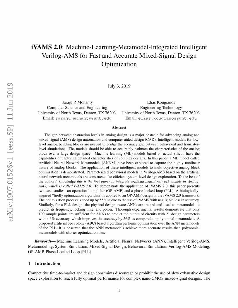
Simulation is an essential part of design verification and optimization. This abstraction level is critical sinceit is the immediate level above the transistor-level netlist and thus determines the accuracy and runtime of thesystem verification/optimization. In the simulation process, parameterized behavioral models for the analogblocks are necessary. Simulating an entire AMS system with transistor-level netlists, though very accurate,is formidable. A common solution is to simulate the AMS system at the behavioral level. Parameterizedbehavioral models share the same design variables as the transistor-level design. When the values of thedesign variables change, the values of the circuit parameters for the behavioral model change accordingly.Thus the impact of the transistor-level design changes on the behavioral level are captured. iVAMS providessuch Verilog-AMS modules, as shown in Fig. 2 [13].

iVAMS is based on a set of artificial neural network (ANN) metamodels. The metamodels are sample-based and fall into two categories: the performance metric metamodel (PMM) and the circuit parametermetamodel (CPM). Given an analog block, PMMs estimate its performance for any point in the designspace. No actual circuit simulation is required in this estimation process. Thus, PMMs provide an ultra-fast way to explore the design space of the analog block. CPMs, on the other hand, estimate the circuitparameters required to construct a macromodel (not a metamodel) for the analog block. By integrating theCPMs into a macromodel and describing them in Verilog-AMS, a parameterized behavioral model, calledmeta-macromodel, can be obtained. A macromodel is usually a white-box or grey-box model [17] that

Page – 4-of-28

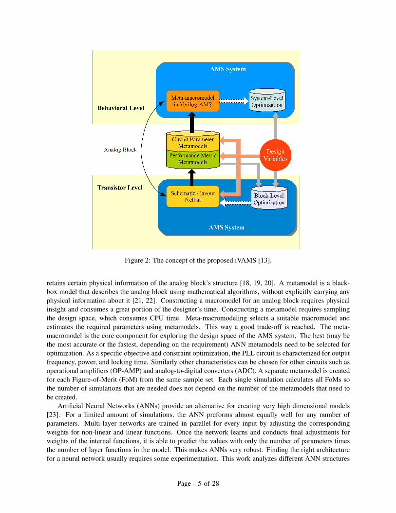
Figure 2: The concept of the proposed iVAMS [13].

retains certain physical information of the analog block’s structure [18, 19, 20]. A metamodel is a black-box model that describes the analog block using mathematical algorithms, without explicitly carrying anyphysical information about it [21, 22]. Constructing a macromodel for an analog block requires physicalinsight and consumes a great portion of the designer’s time. Constructing a metamodel requires samplingthe design space, which consumes CPU time. Meta-macromodeling selects a suitable macromodel andestimates the required parameters using metamodels. This way a good trade-off is reached. The meta-macromodel is the core component for exploring the design space of the AMS system. The best (may bethe most accurate or the fastest, depending on the requirement) ANN metamodels need to be selected foroptimization. As a specific objective and constraint optimization, the PLL circuit is characterized for outputfrequency, power, and locking time. Similarly other characteristics can be chosen for other circuits such asoperational amplifiers (OP-AMP) and analog-to-digital converters (ADC). A separate metamodel is createdfor each Figure-of-Merit (FoM) from the same sample set. Each single simulation calculates all FoMs sothe number of simulations that are needed does not depend on the number of the metamodels that need tobe created.

Artificial Neural Networks (ANNs) provide an alternative for creating very high dimensional models[23]. For a limited amount of simulations, the ANN preforms almost equally well for any number ofparameters. Multi-layer networks are trained in parallel for every input by adjusting the correspondingweights for non-linear and linear functions. Once the network learns and conducts final adjustments forweights of the internal functions, it is able to predict the values with only the number of parameters timesthe number of layer functions in the model. This makes ANNs very robust. Finding the right architecturefor a neural network usually requires some experimentation. This work analyzes different ANN structures

Page – 5-of-28

and internal functions and applies generated metamodels for further multi-objective optimization algorithmsto receive the optimal parameter values. The data to create the ANN are directly generated by SPICE. Oncethe ANN is generated, it can predict the output value very fast, due to its low complexity and simplicity.Hence, the prediction is orders of magnitude faster than SPICE.

3.2 iVAMS 2.0 Generation

Given an analog block, the goal of iVAMS generation is to obtain the artificial neural network metamodels(PMMs and CPMs) and the meta-macromodel integrated Verilog-AMS module. The iVAMS generationflow is shown in Fig. 3. The process starts with determining the design variable ranges and the numberof simulation samples. By sampling the analog block design space with transistor-level simulations, anumber of design variable samples and samples of the circuit’s responses of interest are obtained. Usingthese samples, neural networks with the selected architecture are then trained to accurately model the circuitresponses. If the accuracy is insufficient, the designer can adjust the neural network architecture and/or addadditional samples.

Once the artificial neural network metamodels with sufficient accuracy are obtained, the generatedPMMs can be used in optimizing the analog block. In order to generate a meta-macromodel for theanalog block in Verilog-AMS, a macromodel architecture is selected and implemented in Verilog-AMS.The computation of the circuit parameters for the macromodel is done using CPMs and is embedded in theinitial block of the Verilog-AMS module.

Artificial neural network models are composed of a mass of fairly simple computational elements andrich interconnections between the elements. The ANN generation flow is shown in Figure 4. A trainingdata set is generated using Latin Hyper-Cube Sampling (LHS) and the results are used for ANN training.The verification is conducted using a verification data set that is roughly 30% the size of the training dataset and is generated also using LHS. It is important that the training and verification data sets are distinct.Otherwise the performance of the ANN will be artificially inflated. Statistical fitting data is collected fromboth training and verification data. The best configuration metamodel is selected based on the statisticaldata, as discussed further in this Section.

ANNs operate in a parallel and distributed fashion which may resemble biological neural networks.Most ANNs have some sort of “training” rule by which the weights of the connections are adjusted on thebasis of presented patterns. They normally have great potential for parallelism, since the computations ofthe components are independent of each other. It has been proven in the universal approximation theorem[24] that a neural network with one hidden layer can estimate any continuous function that maps to realnumbers.

3.2.1 Multilayer Artificial Neural Networks (ANNs)

A multiple layer ANN consists of an input, a with nonlinear activation function in hidden layer, and linearactivation function in the output layer (Fig. 5). Multilayer networks are very flexible and powerful due totheir ability to represent nonlinear as well as linear functions. The multilayer ANN needs to have at leastone non-linear function, otherwise a composition of linear functions becomes just another linear function.

The two common nonlinear activation functions that are usually used for the hidden layer are [1]:

bj (vj) =

(1

1 + e−λvj

), or (1)

bj (vj) = tanh(λvj), (2)

Page – 6-of-28

Figure 3: The detailed steps of iVAMS 2.0 generation [9].

where j denotes a neuron in the hidden layer, bj and vj are its input and output, respectively, and λ is theneuron transfer function steepness. The predicted output is given by:

y =d∑j=1

βjbj(vj) + β0, (3)

where βj is the weight in the output due to neuron j, d is the number of neurons in the hidden layer and β0a constant. On the other hand, a linear layer function has the following format:

vi =s∑i=1

wjixi + wj0, (4)

where wji is the weight connection between the jth component in the hidden layer and the ith component ofthe input and wj0 is a constant bias. The ANN training is performed to minimize the least square criterion:

E =n∑k=1

(yk − yk)2, (5)

Page – 7-of-28

Training

Phase

Verification

Phase

Training LHS Training FoM

tanhsigNN logsigNN radialNN

Verification LHS Verification FoM

Statistical FoM Data of the PLL Components

Select most Accurate NN Metamodel of the PLL Components

Figure 4: Flow for generating machine learning (artificial neural network or ANN) metamodel.

where yk and yk are the actual and predicted responses, respectively, at the k-th training point (of n).

3.2.2 Radial Neural Networks

Radial neural networks are also two-layer networks. The first layer has radial base neurons, and calculates itsweighted inputs with distance and its net input with a radial function. The second layer has linear neurons,and calculates its weighted input with a dot product function and its net inputs by combining its weightedinputs and biases. Both layers have biases. The radial network mathematical model is as follows:

y =

N∑i=1

aiρ (‖ x− ci ‖), (6)

where ci is the center vector of neuron i, x is the prediction point, ρ is the neuron’s transfer function and aiare the weighs of the linear neuron. ‖ x− ci ‖ is the Euclidean distance between x and ci.

Initially the radial basis layer has no neurons. The following steps are repeated until the network’s meansquared error falls below the desired goal. The network is simulated. The input vector with the greatest erroris found. A radial basis neuron is added with weights equal to that vector. The linear layer weights are thenrecalculated to minimize the error.

Each neuron in the radial basis layer will output a value according to how close the input vector is toeach neuron’s weight vector. Thus, radial basis neurons with weight vectors quite different from the inputvector have will have outputs near to zero. These small outputs have only a negligible effect on the linearoutput neurons.

In contrast, a radial basis neuron with a weight vector close to the input vector produces a value near 1.If a neuron has an output of 1 its output weights in the second layer pass their values to the linear neurons

Page – 8-of-28

x1

Input Layer

x2

xN

b11

b12

b1M

W1 y

Hidden Layer Output Layer

Neuron

+ f1

+ f1

+ f1

b21

b12

b2M

W2

Neuron

+ f2

+ f2

+ f2

1

y2

yN

Figure 5: Feed forward ANN architecture. N input parameters x using weights for the interface betweenthe hidden (W1) and local layers (W2) functions to produce the output responses yj .

in the second layer.

3.3 Standardizing or Normalizing Data during ML model generation

The data set is generated from the RLCK parasitic aware netlist simulations. It include parasitic resistance(R), parasitic capacitances (C), parasitic self-inductances (L) as well as coupling inductances (K). Theinput data set is the same for every metamodel and is generated using LHS. LHS supports any amountof planes and is proven to work better than Monte Carlo due to the more even distribution of points whilestill incorporating the random factor that helps to detect nonlinearity. LHS divides each plane (parameter)into Latin squares and randomly picks a point from each square. An output is generated for each run fromSPICE simulations saving each needed value to its own data set. Hence, each metamodel has its own targetdata set. This paper targets ANNs that have a single output with multiple inputs.

The validation and test data must be standardized or normalized using the statistics computed from thetraining data. It is desirable to either normalize or standardize the input data as the input dataset typicallyhas a large dynamic range. If not, the training of higher values can outweigh the lower values and the ANNwill not train properly. In this paper, 2 commonly used methods are applied to standardize the data:

1. Normalizing to mean (µ) 0 and standard deviation (σ) 1.

2. Standardizing to midrange 0 and range 2 (from -1 to 1).

3.4 ANN Metamodel Selection Criteria

There may be numerous metamodels created from the same sampled set. The Root Mean Square Error(RMSE) and correlation coefficient R2 are common metrics used for goodness of fit. The RMSE is derived

Page – 9-of-28

from the sum of square errors (SSE):

RMSE =

√1

NSSE (7)

=

√√√√ 1

N

N∑k=1

(y(xk)− y(xk))2, (8)

where y are the actual simulation result values and y are the results of the metamodel at the same location asthe simulation point. R2 is the coefficient of determination, which predicts the probability of a future resultto be predicted by the model and is also used to verify the model accuracy.

The created model may fit perfectly to the training data set but may not qualify as a good model torepresent the output for the given process at other points. For this reason, the verification data set is createdso that the points are at different locations than the original sample. It is a good idea not to use the verificationset for training, since it will defeat the purpose of testing the metamodel on totally unbiased points. If theverification RMSE and R2 values do not differ very much from the training values, then the model has beentrained correctly, otherwise it has not.

3.5 Resolving Over-fitting in iVAMS 2.0

An ML model (including ANN or deep neural network (DNN)) is over-fitted or inflated if the accuracy ofthe DNN model is better than the training dataset [25]. In other words, the ANN/DNN architecture maybe more complex than it is required for a specific problem. Different solutions such as the use of differentdatasets and reduction of the complexity of the ANN/DNN can be deployed. In ML modeling, over-fittingis the phenomenon where the ANN becomes worse instead of improving after a certain point during trainingwhen it is trained to as low errors as possible [26]. This is because excessive training or a large amount ofneurons in the hidden layer may make the network memorize the training patterns and stop adjusting theweights. There are several methods to avoid over-fitting. One method is regularization which tries to limitthe complexity of the network such that it is unable to learn peculiarities. Another method is early stoppingwhich aims to stop training at the point of optimal generalization.

4 Comparative Perspective with Prior Research

The current literature is rich in research attempting to speed up the design process of complex AMS circuits.Design space exploration approaches from high level descriptions of analog circuits are given in [27].Posynomial modeling (a posynomial is a special type of polynomial [28]) for gate sizing is presented in [29].A layout-aware modeling approach for analog synthesis is given in [30]. A single manual design iterationdesign flow is proposed in [31] for fast design optimization of VCOs. In [32], an ABC algorithm is used todetermine the different parameters of a Schottky barrier diode. In [33], the ABC optimization algorithmis investigated considering the transient performance of a CMOS inverter circuit. Swarm intelligencealgorithms including ABC and particle swarm optimization as well as differential evolution and its varianttechniques are used for analog circuit optimization using a CMOS Miller operational transconductanceamplifier in [34].

The following are selected research works that have applied ANNs in VLSI design. In [35], the authorshows that ANNs can be used for circuit analysis. In [36], the authors introduce the creation of ANNsfor estimating the output of operational amplifiers from a high level perspective which does not accountfor parasitics. In [37], optimal and Hopfield binary ANNs are used for testing stuck-at-fault and delayfaults in digital circuits. In [38], ANNs are trained on multi-dimensional mapping between geometricalvariables and the values of independent circuit elements to predict the electromagnetic behavior of vias. In

Page – 10-of-28

[39], the authors propose to speed up simulations by replacing repeated simulation data such as polynomialand look up models with well trained ANNs. In [40], a Hopfield ANN model is used to represent digitalcircuit behavior. In [41], a feed-forward dynamic neural network model is developed for amplifier andmixer circuits directly from input-output large-signal measurements, without having to rely on the internaldetails of the circuit. In [42], ANNs are used for electromagnetic susceptibility analysis and optimization ofelectronic devices.

The iVAMS proposed in this work is built upon neural network metamodels. These intelligentsurrogate models facilitate fast block-level OP-AMP optimization and accurate parameterized behavioralmodeling which enables efficient system-level design exploration. Modeling nano-CMOS AMS circuitsusing metamodeling techniques is becoming popular [16]. Metamodeling OP-AMP performance metricsusing neural networks was studied in [43] for their capability of capturing the highly nonlinear nature ofanalog circuits. More recently, the need for efficient system-level design exploration kindled interest onparameterized macromodeling. In [19], an OP-AMP design space was partitioned and the sub-regions wereapproximated with local low-order polynomials to overcome the strong nonlinearity in large design spaces.

In this work, we apply ANN metamodels to OP-AMP parameterized macromodels (meta-macromodels)to avoid design space partitioning. Moreover, this ANN based meta-macromodel is implemented in Verilog-AMS for practical behavioral simulations. Using neural networks for behavioral modeling has been exploredin the literature, e.g., [44, 45]. Nevertheless, actual implementation of such neural networks for AMS circuitsin a hardware description language (HDL) has not been presented. From other related research, the closestone to this work is [46]. However, it implemented a neural network with built-in training algorithm but nota behavioral model for any common analog circuit. Thus from our discussion, the current contribution ofiVAMS is unique and practical.

5 iVAMS 2.0 Case Study: An Operational Amplifier (OP-AMP)

We apply iVAMS to the fully differential op amp shown in Fig. 6, which is based on a 90nm CMOS processand a 1-V supply. It consists of a folded-cascode operational transconductance amplifier (OTA), a common-source (CS) amplifier, and a common-mode feedback (CMFB) circuit. Section 5.1 describes the generationof artificial neural network metamodels for the OP-AMP along with their accuracy evaluations. Section 5.3presents a multi-objective OP-AMP optimization using the generated iVAMS PMMs. A meta-macromodelin Verilog-AMS for the OP-AMP is constructed in Section 5.2 using the iVAMS CPMs.

5.1 OP-AMP iVAMS 2.0 Metamodel Generation

The performance metrics of interest for this OP-AMP are the open-loop DC gain (A0), bandwidth (BW ),phase margin (PM ), slew rate (SR), and power dissipation (PD). Metamodels for these metrics weregenerated for iVAMS block-level optimization. In order to construct a meta-macromodel for system-leveldesign exploration, metamodels for the circuit parameters used in the macromodel are also required. Thesecircuit parameters include the transconductance gm, and the positive and negative maximum availablecurrents Ip and In of the OP-AMP input stage. As a specific example, an ANN architecture with a singlehidden layer is chosen for the metamodels [47].

The input layer, x, is a vector of the OP-AMP design variables which include the bias current and thetransistor widths and lengths. There are thirty transistors in the OP-AMP design. By properly grouping thetransistors, we have sixteen design variables (N = 16). For example, the current mirror devices M1–M4in Fig. 6 should all have the same size, therefore two variables, instead of eight, are used. In this work, thehidden layer consists of four neurons (M = 4) with hyperbolic tangent function as the activation functionf1. The output layer is a single neuron employing a linear activation function f2. The model output y is oneof the performance metrics or circuit parameters. W1 is a matrix composed of the weights of the connections

Page – 11-of-28

Figure 6: The schematic of the OP-AMP case study [9].

from the design variables in the input layer to the neurons in the hidden layer. Similarly, W2 is formed bythe weights of the connections from the hidden layer to the output layer. Additional control on each neuronis through bias bij (i = 1, 2 and j = 1, 2, ...,M ). The artificial neural networks were trained using 500samples with Bayesian Regulation training. It may be noted that, while different mathematical functioncan be be used for metamodeling, an ANN used in the current paper for it Verilog-AMS integration as theANN is accurate and capable of modeling complex systems [26]. The number of simulations needed togenerate metamodels is significantly lower than those needed for actual netlist simulation [16]. At the sametime, design exploration over metamodels is significantly faster than the simulations over netlists in SPICE.Thus, in summary the ANN metamodel integrated Verilog-AMS is ultra-fast while maintaining circuit-levelaccuracy.

In order to evaluate the accuracy of the iVAMS metamodels, a verification set consisting of 2000samples of design variable and circuit response pairs were generated. It may be needed that this samplingis for verification purposes only and need not be used when iVAMS is used in design flow. The outputy computed by the metamodel is compared with the “true” output y obtained from the transistor-levelsimulation. To comparatively assess the proposed iVAMS ANN metamodels, we generated second-orderpolynomial (PO) metamodels and compared their accuracy using the coefficient of determination (R2),relative maximum absolute error (RMAE), root relative square error (RRSE), and root mean square error(RMSE). RMSE measures the overall error in terms of the unit of the modeled output. RRSE expresses thisoverall error relative to the standard deviation of the true output [48]. RMAE assesses the model locally andfinds the maximum relative error [49]. R2 measures the model quality globally with respect to the varianceof the true output. An accurate model should have small RMAE, RRSE, and RMSE. Its R2 value should beclose to 1. The results are listed in Table 1.

The ANN metamodels achieve higher accuracy overall except for A0. For some circuit responses (e.g.,PM , Ip, and In), the PO metamodels deliver poor accuracy, while the ANN metamodels attain reasonableaccuracy. Another advantage of the ANN metamodels over the PO metamodels is that their accuracy canbe further improved by adding more neurons to the hidden layer, without drastically increasing the modelcomplexity. All ANN metamodels in this work employ a 4-neuron hidden layer for simplicity. In practice,

Page – 12-of-28

Table 1: Accuracy of The OP-AMP iVAMS Metamodels [9].

Metamodel Accuracy Metric

Output Type R2 RMAE RRSE RMSE

A0NN 0.959 1.324 0.202 41.93 V/V

PO 0.973 1.044 0.163 33.78 V/V

BWNN 0.987 0.894 0.116 2.12 kHz

PO 0.986 0.965 0.117 2.14 kHz

PMNN 0.901 2.161 0.317 4.99o

PO 0.348 4.466 0.807 12.70o

SRNN 0.989 0.483 0.105 0.292 mV/ns

PO 0.985 0.662 0.119 0.332 mV/ns

PDNN 0.996 0.523 0.062 8.306 µW

PO 0.980 1.314 0.141 18.817 µW

gmNN 0.999 0.106 0.018 1.769 µA/V

PO 0.999 0.101 0.021 1.973 µA/V

IpNN 0.991 0.675 0.095 0.311 µA

PO 0.729 3.407 0.521 2.506 µA

InNN 0.994 0.494 0.080 0.261 µA

PO 0.749 3.727 0.501 2.412 µA

adaptively adjusting the hidden layer size is recommended to find the optimal model.

5.2 OP-AMP iVAMS 2.0 Meta-Macromodel Construction

An OP-AMP meta-macromodel can facilitate fast system-level design exploration. Meta-macromodelconstruction starts with macromodel selection. Some OP-AMP macromodels that can be used include thestructural model in [18], the linear time-invariant (LTI) model in [19], and the symbolic model in [20]. Weadopted a symbolic model similar to the one in [20] since it not only models the OP-AMP small-signalbehavior but also its large-signal behavior such as slew-rate limitation. This model, combined with theiVAMS CPMs to form the OP-AMP meta-macromodel, is shown in Fig. 7.

Figure 7: The iVAMS 2.0 OP-AMP meta-macromodel [9].

The two-stage model in Fig. 7 takes into account the slew-rate effect due to the limited maximum avail-

Page – 13-of-28

able positive and negative currents Ip and In. These circuit parameters, together with the transconductanceof the first stage gm and the OP-AMP small-signal function H(s), are functions of the design variables.They are estimated using the iVAMS CPMs. These CPMs all have the same ANN architecture. With f1being a hyperbolic tangent function and f2 being a pure linear function, this architecture can be expressedmathematically as:

y = b21 +M∑j=1

w2,j · tanh

(b1j +

N∑i=1

w1,ij · xi

), (9)

where w1,ij ∈ W1 and w2,j ∈ W2. Implementing this equation in Verilog-AMS is an essential step ofbuilding the iVAMS meta-macromodel. An example is shown in Algorithm 1. After training the neuralnetworks for the CPMs, the neural network weights and biases are stored in text files. In the initialblock of the OP-AMP Verilog-AMS module, these weights and biases are read from the files, and thefunction nn_metamodel computes the circuit parameter values for the meta-macromodel. The computedcircuit parameter values are used in an analog process in the Verilog-AMS module to realize the model inFig. 7. The OP-AMP small-signal function can be described using a function such as laplace_nd.

The quality of the meta-macromodel relies on the accuracy of the CPMs and the suitability of the selectedmacromodel. In order to validate the iVAMS meta-macromodel, simulations using the constructed Verilog-AMS module were compared with those using the SPICE model. The design variable values were set to bethose of the selected optimal design in Section 5.3. The results of the AC analysis are shown in Fig. 8. Thedifference seen in the frequency responses can be reduced by adaptively adjusting the neural network hiddenlayer sizes instead of using a fixed value. The OP-AMP step response is shown in Fig. 9. The DC behaviorand gain are shown in Fig. 10. These simulations demonstrate that an effective OP-AMP meta-macromodelhas been constructed.

100

101

102

103

104

105

106

107

108

109

−40

−20

0

20

40

60

Gai

n (

dB

)

100

101

102

103

104

105

106

107

108

109

−180

−135

−90

−45

0

Frequency (Hz)

Ph

ase

(deg

)

SPICE

iVAMS

Figure 8: AC analyses of the OP-AMP [9].

Page – 14-of-28

Algorithm 1 Verilog-AMS code for the OP-AMP artificial neural network (ANN) metamodels [9].

function real nn_metamodel;integer w1, w2, b1, b2, i, j, readfile,...;real w, b, v, u;// Read metamodel weights and bias from// text files w1, w2, b1, and b2.beginw1 = $fopen("w1.txt", "r");w2 = $fopen("w2.txt", "r");b1 = $fopen("b1.txt", "r");b2 = $fopen("b2.txt", "r");v = 0.0;for (j = 0; j < nl; j = j + 1)beginu = 0.0;for (i = 0; i < size_x; i = i + 1)beginreadfile = $fscanf(w1, "%e", w);u = u + w * x[i];endreadfile = $fscanf(w2, "%e", w);readfile = $fscanf(b1, "%e", b);v = v + w * tanh(u + b);endreadfile = $fscanf(b2, "%e", b);nn_metamodel = v + b;$fclose(w1);$fclose(w2);$fclose(b1);$fclose(b2);endendfunction

0 100 200 300 400 500

0

0.2

0.4

0.6

0.8

1

Time (ns)

Vo

ltag

e (V

)

Inp

Outp (SPICE)

Outp (iVAMS)

Figure 9: Transient simulations of the OP-AMP with a step input.

Page – 15-of-28

−100 −60 −20 20 60 100

0

0.2

0.4

0.6

0.8

1

Dif

fere

nti

al O

utp

uts

(V

)

Outp Outn

−100 −60 −20 20 60 100

0

100

200

300

400

500

600

DC differential input amplitude (mV)

Gai

n (

V/V

)

d(Voutp

− Voutn

) / d VIN

Figure 10: The DC behavior and gain of the OP-AMP.

5.3 OP-AMP iVAMS 2.0 Multi-objective Optimization

In this section, we demonstrate block-level optimization for the OP-AMP design using the iVAMS PMMs.Here, the OP-AMP is required to have high slew rate while consuming minimum power. Thus theoptimization problem is to maximize SR and to minimize PD, constrained by the requirements forA0, BW, and PM. An effective approach to this problem is to find the Pareto front (PF) that consistsof a set of non-dominated solutions for the optimization problem. The designer can then select one designfrom this solution set to implement. Metaheuristic algorithms have shown promising results in solvingmulti-objective analog circuit optimization problems. For example, a particle swarm optimization (PSO)was used in [50]; a memetic search based algorithm was used in [51]; and a differential evolution (DE)based algorithm is used in [52]. In this study, a multi-objective firefly algorithm (MOFA) belonging tothe same category is used. It mimics the behavior of tropic firefly swarms that are attracted toward flieswith higher flash intensity. Preliminary studies show that its performance could surpass existing establishedmulti-objective algorithms [53]. The iVAMS-assisted OP-AMP MOFA proposed in this work in shown inAlgorithm 2.

The goal of the algorithm is to find K Pareto points that constitute the PF through a predeterminednumber of iterations, tmax. The algorithm starts with K randomly generated designs. In each iteration, theperformance of the K OP-AMP designs are estimated using the iVAMS PMMs. If non-dominated designsare found, move vectors from each current design toward the non-dominated designs will be computed basedon the attractiveness of these designs and the characteristic distance [53]. If no non-dominated designsare found, a move vector toward a current best design determined by the combined weighted sum of theobjectives, ψ(x), is computed for each current design. SR(x) and PD(x) are the slew rate and powerdissipation for a design x estimated using the iVMAS PMMs, and are normalized with respect to their ownsample mean and standard variation. The current designs will be moved to new locations within the design

Page – 16-of-28

Algorithm 2 iVAMS-Assisted Firefly based OP-AMP Multi-objective Optimization.1: Current iteration t← 0;2: Initialize a vector of K designs X = {x1,x2, ...,xK};3: while t < tmax do4: Evaluate OP-AMP performance for all designs in X using iVAMS PMMs;5: Find non-dominated designs Xnd ⊂ X;6: for i = 1 to K do7: if No non-dominated designs are found then8: Generate random weight w ∈ [0, 1];9: Find a best design x∗ ∈ X that maximizes ψ(x) = (1− w) · SR(x)− w · PD(x);

10: Compute a move vector ∆xi for xi toward x∗;11: else12: Compute a move vector ∆xi for xi toward Xnd;13: end if14: Constraint1 ← A0(xi + ∆xi) > A0min;15: Constraint2 ← BW (xi + ∆xi) > BWmin;16: Constraint3 ← PM(xi + ∆xi) > PMmin;17: if Not all constraints are satisfied then18: Generate a new move;19: end if20: end for21: Let ∆X = {∆x1,∆x2, ...,∆xK};22: X← X + ∆X;23: t← t+ 1;24: end while

space using the computed move vectors. The PMMs are then used to check whether the new designs satisfythe constraints. If not, new moves will be generated. The optimization specifications and an arbitrarilyselected optimal design from the PF of a MOFA optimization are shown in Table 2.

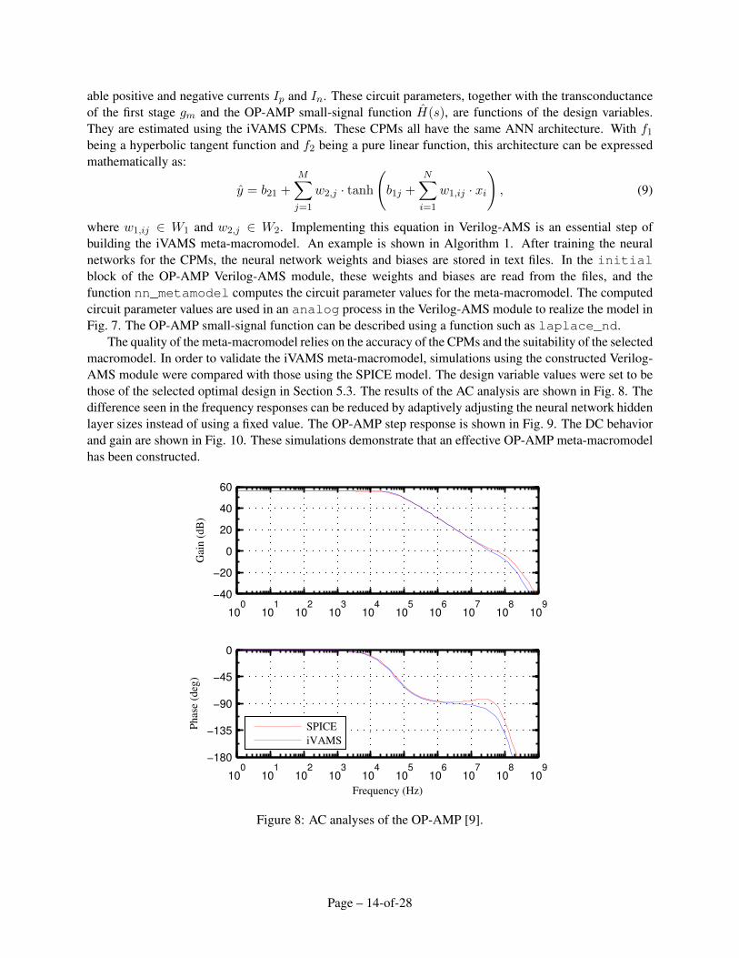
The MOFA has been implemented in MATLAB. Three optimization runs have been performed. The firstrun is aimed at finding the true PF. In order to approximate the true PF, K and tmax have to be sufficientlylarge. In this run, K = 50 and tmax = 5000 were set experimentally. Although these numbers are large, theruntime for this optimization is small thanks to the neural network iVAMS PMMs. To compare the iVAMS-assisted MOFA (iVAMS-MOFA) with the same algorithm using SPICE models (SPICE-MOFA) to evaluatethe OP-AMP performance, we may run a similar optimization. However, running MOFA using SPICE(SP) models with such large K and tmax would be extremely time consuming. Therefore, we alternativelydecreased there numbers to K = 20 and tmax = 500 and performed two optimization runs to compare thespeed of iVAMS-MOFA and SPICE-MOFA. These three optimizations are summarized in Table 3. It canbe seen that the iVAMS-MOFA is 5580 times faster than the SPICE-MOFA. The PFs generated by thethree optimizations and the arbitrarily selected OP-AMP design are shown in Fig. 11.

6 iVAMS 2.0 Case Study: A Phase-Locked Loop (PLL)

This section presents ML modeling and optimization of a PLL through an ANN-based metamodel [26]. Fornon-polynomial metamodeling different architectures of neural networks are considered to perform trade-off analysis between speed and accuracy. As a practical demonstration of the use of the non-polynomialneural network metamodels, the physical design optimization of a 180 nm CMOS PLL is undertaken. A

Page – 17-of-28

Table 2: OP-AMP Design Optimization [9].

Selected Optimal DesignPerformance Constraint Predicted True

A0 (dB) > 43 56.4 55.7

BW (kHz) > 50 56.8 56.7

PM (degree) > 70 81.9 88.5

Objective

SR (mV/ns) Maximized 5.54 5.49

PD (µW) Minimized 85.11 85.77

Table 3: Comparison of MOFA OP-AMP Optimizations

Optimization # 1 2 3

Model Type ANN ANN SPICE

Number of Pareto Points, K 50 20 20

Number of Iterations, tmax 5000 500 500

Runtime 0.57 h 84.63 s 131.18 h

Normalized Speed – ×5580 1

biologically inspired tool, the ABC algorithm is used for optimization of the PLL physical design that usesthe metamodels instead of the actual circuit (i.e. the parasitic aware netlist). It is demonstrated that thenon-polynomial neural network metamodel assisted optimization is faster and more accurate compared tothe polynomial metamodel.

The phase locked loop (PLL) is a closed feedback loop system which is implemented as shown in Fig.12. The detailed baseline design of this circuit is discussed in [1, 54]. The physical design is shown inFig. 13. A parasitic-aware netlist, including resistance (R), capacitance (C) and inductance (both self andmutual) (LK) is extracted from the layout. The netlist is then parameterized and used for simulations for theinput data sets for each metamodel. Once the data are received from SPICE simulations, they are processedby an external tool (Matlab). SPICE simulation results of the circuit are shown in Fig. 14, which showsthe frequency over time plot, with the PLL locking in 24.58 µs. The baseline phase noise diagram in Fig.15 shows that the circuit has acceptable phase noise, (-163 dBc/Hz at 10 Hz offset). The average powerconsumption of the PLL is 9.28 mW.

6.1 PLL iVAMS 2.0 Metamodel Generation

Given that each SPICE simulation for the PLL circuit takes approximately 10 minutes to converge, theamount of simulation runs are limited. In this work 100 simulations for training and 30 simulations forverification have been chosen. Different architectures of ANNs are evaluated. For feed-forward networkstwo differentiable transfer functions (tanh - tansig, and logarithmic - logsig) are used for the hidden layer. Inaddition, the experimental results also consider the difference between raw regular input data in comparisonto normalized and standardized input sets.

The verification data set is also chosen using LHS, but it is ensured that none of the points match the

Page – 18-of-28

50 75 100 125 150 175 200 225 250

2

3

4

5

6

7

8

9

10

11

12

Sle

w R

ate

(mV

/ns)

Power Dissipation (µW)

NN, K = 50, tmax

= 5000

NN, K = 20, tmax

= 500

SP, K = 20, tmax

= 500

Selected optimal design

Figure 11: Pareto fronts from MOFA OP-AMP optimization [9].

LC−VCOPhase Detector

(PD)

Clock Out

ReferenceClock In Charge Pump

Loop Filter (CP)

Frequency Divider2

Figure 12: Block diagram of a phase locked loop (PLL) [26].

111111

11111

11

1111

1111111

1111111111

1111

111111

111111 11111111111111111111111111111111 1111111111111111111111111111 11111111 111111111111111111

11111111111

1111111111111111111

11

111111111111

111

111111111

1111111

11111111

1

11

11111111

111111111

1

11

11111111

111111111111 111111111111 11111111 11111111111111111111111111111111 111111111111 1111111111 111111 111111111111 11111111111111111111 11111111 11111111111111111111111111111111 11111111 111111111111 11111111 111111111111 11111111111111111111 11111111111111111111111111111111111

1111 1111111111111111111111111111111111111111111111111111111

1111111111

111111111111111111111111111111111111111111111111111111111111111111111111111111111111111111111111111111111111111111111111111111111111111111111111

111

1111111

11111111111

1111111111111111111111111111111111111111111111111111111111111111111111111111111111111111111111111111111111111111

111111

111111111

1111 1111

1111

1111111111111111

11

11

11

11

11

111111111111

111

1111

11

1111

1

1111

1

1

1111111111

11

11

1111 11111 1111111111111 1111111 1111111111 11

111 1111111111 111111111 11 11111111111111111

111111

11111111111111111111111111111111111111111111111111111111111

111111111111111111111111111111111111111111111111111111111111

1111 11111111111111111111111111111111 1111111111111111111111 11111111 11111111111111111

1111 11111

1111111111111111111111111111111111111111111111111111111111111111111111111111

111

1111111

111

1111111111111111111111111111111111111111111111111111111111111

111111

111111111

1111 1111

1111

111111111111111111

11

11

11

11

11

111111111111

111111111

111111111111

1

11111111

11

111111111111

1111

1111

11111

1111

111111111111

11111

111

1111111111111

111111

1111111111111

11111111

1111

111111111111111

1111

1111

11111111111111111111111111111111111111

111111

11111111

11111

11111

11

1111

111111111111111111111111111111111

1111

1

111

1

1111

11

1111

111111

111111111111111111

11111111

111111

11111

1111111111

111111111111111111111111111111111

11

111111

1111111111111111111

11111111111111111111111111111111111111111111111111111111111111111111111111111111111111111111111111111111111111111111111111111111111111111111

111

11111111111 1111111111111111111111111111111111111111111

111111111111111111111111111111111111111111111111111111111111111111

111111

111111111111

1111 1111

1111

1111

11

1111111111111111

1

11

11

11

11

111111111111

111111111111

1

111111

11111111

11

1

11111111111

111

111111111111

1111

11

1

1111111111

111

11

11111111

11111

11111111111111111111

11111111

1

111111111

111111

111111

1111

111111

1111

111111111

111111

111111111

111111

111111

1111

111111

1111

111111111

111111

111111111

111111

111111

1111

111111

1111

1

111111

111111

111111111111111111111111111111111111111111111

1111

1111111111

1111

111111

1111

11

111111

1

111111111111

1

111111

111111

111111

1111

111111

1111

111111111

111111

111111111

111111

111111

1111

111111

1111

111111111

111111

111111111

111111

111111

1111

111111

11111

111

111111111111111111111111

11111111111111111111111111111111111111111111111111

111111111111111111111 11111111111111

11111

11111

1111111111

111111111111

11111

11111

1111111111

11111

11111

11111

11111

11111

1111111

111111111111

1111111

1111

111111

1111

1111

111111

1111

111111

111111

111111111

111111

1111

1111

111111

1111

111111

111111

111111111

111111

1111

1111

111111

1111

11111111111111111111111111111111111111111111111111111111111111111111111111111111111111111111111111

1111111111111111111111111111111111111111111111111111111111111111111111111111111111111111111111111111111111111111111111111111111111111111111111111111111111111111111111111111111111111111111111111111111111111111111

1111111111111111111111111111111111111111111111111111111111111111111111111111111111111111111111111111111111111111111111111111111111111111111111111111111111111111111111111111111111111111111111111111111111111111111111111111111111111111111111111111111111111111

1111111111111111111111111111111111111111111111111111111111111111111111111111111111111111111111111111111111111111111111111111111111111111111111111111111111111111111

11111111111111111111111111111111111111111111111111111111111111111111111111111111111111111111111111111111111111111111111111111111111111111111111111111111

111111111111111111111111111111111111111111111111111111111111111111111111111111111111111111111111111111111111111111111111111111111111111111111111111111111111111111111111111111111111

1111111111111111111111111111111111111111111111111111111111111111111111111111111111111111111111111111111111111111111111111111111111111111111111111111111111111111111111111111111111111111111111111111111111111111111111111111

111111

1

111111

1111

Figure 13: Physical design of the PLL with area 525×326 µm [26].

Page – 19-of-28

0 0.5 1 1.5 2 2.5 3 3.5x 10

−5

2.7

2.75

2.8

2.85

2.9

2.95x 109

Time (s)

Fre

quen

cy (

Hz)

Frequency Plot

Figure 14: Locking behavior of the PLL circuit [26].

100

101

102

103

104

−175

−170

−165

−160

−155

Frequency (Hz)

dB

c/H

z

Phase Noise of PLL

Figure 15: Phase noise of the baseline PLL circuit [26].

training set. After the neural network training is completed, the input values for the verification set are fedinto the network and the RMSE value is calculated for the verification set. The R2 values are calculatedfor training and verification sets for each combination of the above neural networks. Selected results aresummarized in Tables 4 and 5. The statistics of the best created polynomial functions that were created from[54] are listed in the last rows of the tables for comparison purposes.

For comparison purposes, the data was fitted into partial polynomial equations. Since the full polynomialfunction would result in a very large number of coefficients for 21 variables, partial polynomial functions oforder 1 through 6 are considered. Further, the stepwise regression method is used to filter out the coefficientsthat do not contribute to the function’s outcome.

From the data it is observed that neural networks with no standardization of the input data performthe worst. Even though polynomials show best results without standardization or normalization, this is notthe case for neural networks. Also, it can be concluded that ANNs perform better fitting for this circuit,mostly because of the non-linear flexibility of the ANNs. The data also demonstrates which architecture andnormalization or standardization should be used, i.e. which has the best performance.

6.2 PLL iVAMS 2.0 based Multi-objective Optimization

The proposed design flow using non-polynomial metamodels is shown in Fig. 16. Once the initial physicaldesign netlist is parameterized, the design space is sampled using LHS. The ANN is trained from thesampled data. After the ANN is created and verified for accuracy, the optimization algorithm is appliedto find the optimal parameters. The non-polynomial metamodels are created for each output set of the

Page – 20-of-28

Table 4: Frequency Non-Polynomial Metamodel Comparison of the PLL [26].

Function Data Filtering R2-test R2- verification RMSE Neuronslogsig→purelin none 0.802 0.723 52.74 MHz 4tansig→purelin none 0.839 0.713 51.24 MHz 3radial→purelin none 0.020 0.490 81.51 MHzlogsig→purelin minmax 0.917 0.664 48.89 MHz 9tansig→purelin minmax 0.855 0.699 53.65 MHz 1radial→purelin minmax 0.844 0.712 50.88 MHzlogsig→purelin meanstd 0.843 0.733 53.60 MHz 1tansig→purelin meanstd 0.793 0.762 51.64 MHz 5radial→purelin meanstd 0.848 0.749 48.97 MHz

Data Filtering R2 Order RMSE Number of Coefficientspolynomial none 0.930 4 77.96 MHz 48

Table 5: Locking Time Non-Polynomial Metamodel Comparison of the PLL [26].

Function Data Filtering R2-Test R2-Verification RMSE Neuronslogsig→purelin none 0.828 0.873 1.30 µs 1tansig→purelin none 0.850 0.723 1.44 µs 9radial→purelin none 0.078 0.830 2.26 µslogsig→purelin minmax 0.826 0.870 1.29 µs 1tansig→purelin minmax 0.839 0.942 1.12 µs 10radial→purelin minmax 0.931 0.508 1.65 µslogsig→purelin meanstd 0.826 0.906 1.22 µs 2tansig→purelin meanstd 0.737 0.939 1.12 µs 3radial→purelin meanstd 0.963 0.691 1.23 µs

Data Filtering R2 Order RMSE Number of Coefficientspolynomial none 0.877 4 1.91 µs 56

design. Computationally expensive optimization algorithms can be applied using the fast non-polynomialmetamodels as they are ultra fast compared to the actual netlist simulations. The optimized values are thenused to adjust the initial physical layout to create the near optimal design. This design flow only uses twoiterations for the physical design, at the beginning and the end. Overall, the design flow is as accurate as theparasitic-aware netlist of the circuit but ultra-fast due to the metamodel abstraction, which in turn minimizesthe amount of time the designer needs to spend on the design optimization of the circuit.

The best (may be the most accurate or the fastest, depending on the requirement) non-polynomialmetamodels from the previous section need to be selected for optimization. The optimization algorithmthat is being used is the Artificial Bee Colony algorithm (ABC). ABC is the artificial representation of a beecolony behavior as bees try to find the best food source [55, 56]. More information about the algorithm inthe context of AMS circuit optimization can be found in our previous research [54]. Many metaheuristicalgorithms are based on the swarm intelligence that can be found in nature. It was observed that innature, honey bees are very efficient in finding enriched food sources by splitting tasks and communicatinginformation amongst themselves. The artificial bee colony algorithm closely represents their behavior.All the bees in a colony can perform three different tasks: worker, onlooker and scout. The bees work

Page – 21-of-28

Input Specifications

Create Logical Design

and Physical Design

Perform DRC/LVS/RCLK Extraction

Parametarize Parasitic Netlist

with Design Variables

Perform LHS Sampling

Perform Bee Colony

Optimization Using Metamodels

Done

Specifications

Met?

Parasitic Aware

Parameterized Netlist

Dataset for Sample Points

Optimal Design

Variable Values

Final Optimized Layout

Netlist with Parasitics

No

Yes

YesNo

Adjust Physical Design

Perform DRC/LVS/RCLK

Final Extraction and Simulation

Train Feed Forward

Neural NetworkMultiple Metamodels

Verify Feed Forward

Neural Network MetamodelsMetamodels

Specifications

Met?

Figure 16: Proposed design flow utilizing feed-forward ANN metamodels and the ABC optimizationalgorithm.

Page – 22-of-28

independently and only communicate the information when they come back to the nest. When the bee is inthe scout state, it travels to a random location and brings back information of how valuable the food sourceis. Bees in the worker state travel to the best known location and their whereabouts to collect food. The beesin the onlooker state, are located at the nest and based on the information of scout and worker bees decideto go and forage food or stay back.

This algorithm was found to be effective for use on AMS circuits with metamodels. As a specificobjective and constraint optimization, the PLL circuit is characterized for output frequency, power, andlocking time. A separate metamodel is created for each Figure-of-Merit (FoM) from the same sample set.Each single simulation calculates all FoMs so the number of simulations that are needed does not depend onthe number of the metamodels that need to be created.

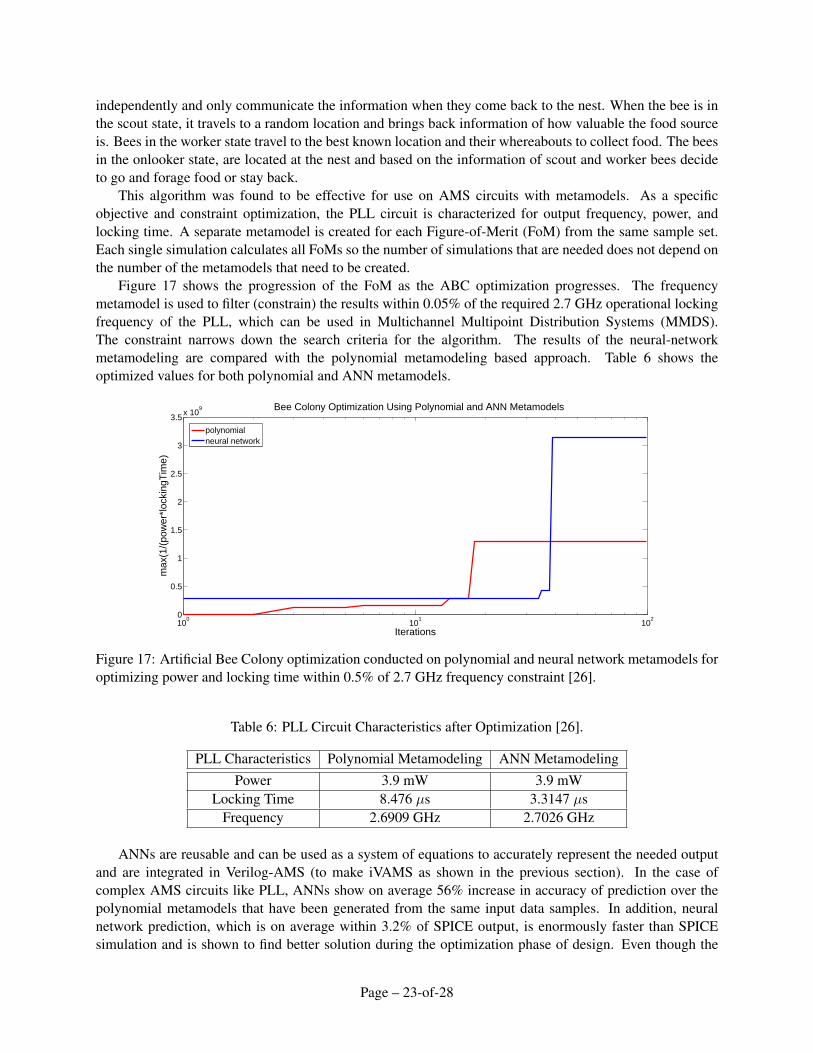
Figure 17 shows the progression of the FoM as the ABC optimization progresses. The frequencymetamodel is used to filter (constrain) the results within 0.05% of the required 2.7 GHz operational lockingfrequency of the PLL, which can be used in Multichannel Multipoint Distribution Systems (MMDS).The constraint narrows down the search criteria for the algorithm. The results of the neural-networkmetamodeling are compared with the polynomial metamodeling based approach. Table 6 shows theoptimized values for both polynomial and ANN metamodels.

100

101

102

0

0.5

1

1.5

2

2.5

3

3.5x 10

9

Iterations

max

(1/(

pow

er*l

ocki

ngT

ime)

Bee Colony Optimization Using Polynomial and ANN Metamodels

polynomialneural network

Figure 17: Artificial Bee Colony optimization conducted on polynomial and neural network metamodels foroptimizing power and locking time within 0.5% of 2.7 GHz frequency constraint [26].

Table 6: PLL Circuit Characteristics after Optimization [26].

PLL Characteristics Polynomial Metamodeling ANN MetamodelingPower 3.9 mW 3.9 mW

Locking Time 8.476 µs 3.3147 µsFrequency 2.6909 GHz 2.7026 GHz

ANNs are reusable and can be used as a system of equations to accurately represent the needed outputand are integrated in Verilog-AMS (to make iVAMS as shown in the previous section). In the case ofcomplex AMS circuits like PLL, ANNs show on average 56% increase in accuracy of prediction over thepolynomial metamodels that have been generated from the same input data samples. In addition, neuralnetwork prediction, which is on average within 3.2% of SPICE output, is enormously faster than SPICEsimulation and is shown to find better solution during the optimization phase of design. Even though the

Page – 23-of-28

circuit that this paper uses as an example is parameterized with 21 parameters, in future work higher andmore complex circuits that can have hundreds of parameters will be investigated.

7 Conclusion and Future Research

The circuit-level accurate behavioral modeling framework called iVAMS has been presented in this article.The machine learning based artificial neural network integrated intelligent Verilog-AMS is called iVAMS2.0 in this article (the predecessor iVAMS 1.0 is polynomial metamodel integrated Intelligent Verilog-AMS). The creation of an iVAMS module for an OP-AMP and PLL have been discussed. The use of theiVAMS for block-level optimization has been demonstrated using a novel multi-objective firefly algorithm.Construction of parameterized behavioral models using iVAMS is also exemplified through an OP-AM casestudy. Future research includes enhancing iVAMS 2.0 with yield-estimation capability to address variabilityof nanometer circuits. For nanoelectronics design, manufacturing process variation is a key design issue asit affects device parameters and eventually chip yield. This paper also presented the generation and usage ofANN metamodels of a PLL. The arificial bee colony algorithm with both non-polynomial and polynomialmetamodels has been used for optimization.

It is a fact that while ML models are attractive options for a variety of modeling applications, the trainingtime, energy, and computational resource requirements are huge [57, 58]. Thus, speeding up the trainingprocess as well as generating sufficiently complex models that represent the circuits and system behaviorwell while execute with minimal resources can be crucial. We intend to present iVAMS 3.0 that willincorporate a hierarchical modeling approach to speed up ML modeling. The future research of iVAMSwill include metamodeling while accounting for process variations and will model statistical parameters ofthe circuits and system characteristics.

In big application domains such as smart cities [59], the large amount of data (aka bigdata) can belive (e.g. real-time sensors) as well as residing in various locations. However, the silicon data involvedin the hardware design phase while complex, is not necessarily live or distributed. A designer typicallydeals with silicon data during or after the end of SPICE simulations, and of one design. Thus, distributedlearning (including federated learning from Google) can have usage for smart city kind applications [60].However, in the case of silicon bigdata involved in hardware design exploration hierarchical learning maybe more useful to reduce the training time, which translates to reduction in design time and non-recurrentcost. However, the distributed paradigm for training of silicon data can also be explored to reduce trainingtime and design cost.

Acknowledgments

A preliminary version of this research appeared in the following peer-review conference [9, 26]. It wasalso presented in work-in-progress poster session in DAC 2013 [10]. The authors would like to thank UNTgraduates Dr. Geng Zheng and Dr. Oleg Garitselov for their help on earlier versions of this work.

References

[1] S. P. Mohanty, Nanoelectronic Mixed-Signal System Design. McGraw-Hill Education, 2015, no.9780071825719.

[2] S. P. Mohanty and E. Kougianos, “Incorporating manufacturing process variation awarenessin fast design optimization of nanoscale CMOS VCOs,” IEEE Transactions on SemiconductorManufacturing, vol. 27, no. 1, pp. 22–31, 2013.

Page – 24-of-28

[3] D. Buffeteau, D. Morche, and J. Gonzáez-Jiménez, “VCO Verilog AMS Model for Fast Simulationin VCO-Based ADC,” in Proc. 28th International Symposium on Power and Timing Modeling,Optimization and Simulation (PATMOS), July 2018, pp. 19–22.

[4] S. P. Mohanty, E. Kougianos, and G. Zheng, “Intelligent metamodel integrated Verilog-AMS for fastand accurate analog block design exploration,” May 5 2015, uS Patent 9,026,964.

[5] S. P. Mohanty, J. Singh, E. Kougianos, and D. K. Pradhan, “Statistical DOE–ILP based power–performance–process (P3) optimization of nano-CMOS SRAM,” Integration Journal, vol. 45, no. 1,pp. 33–45, 2012.

[6] S. P. Mohanty and E. Kougianos, “Methodology for nanoscale technology based mixed-signal systemdesign,” Jun. 9 2015, uS Patent 9,053,276.

[7] S. P. Mohanty, “Ultra-Fast Design Exploration of Nanoscale Circuits through Metamodeling,” Apr. 272012, invited Talk, Semiconductor Research Corportation (SRC), Texas Analog Center for Excellence(TxACE).

[8] M. Kotti, M. Fakhfakh, and E. Tlelo-Cuautle, “Kriging Metamodeling-Assisted Multi-ObjectiveOptimization of CMOS Current Conveyors,” in Proc. 15th International Conf. Synthesis, Modeling,Analysis and Simulation Methods and Applications to Circuit Design, July 2018, pp. 293–296.

[9] G. Zheng, S. P. Mohanty, E. Kougianos, and O. Okobiah, “iVAMS: Intelligent Metamodel-IntegratedVerilog-AMS for Circuit-Accurate System-Level Mixed-Signal Design Exploration,” in Proceedingsof the 24th IEEE International Conference on Application-specific Systems, Architectures andProcessors (ASAP), 2013, pp. 75–78.

[10] G. Zheng, S. P. Mohanty, and E. Kougianos, “iVAMS: Intelligent Metamodel-Integrated Verilog-AMS for Fast Analog Block Optimization,” in Work-in-Progress Session Poster, Design AutomationConference, 2013.

[11] M. J. Krasnicki, R. Phelps, J. R. Hellums, M. McClung, R. A. Rutenbar, and L. R. Carley, “ASF:a practical simulation-based methodology for the synthesis of custom analog circuits,” in Proc.IEEE/ACM Int. Conf. Computer Aided Design (ICCAD), 2001, pp. 350–357.

[12] H. Graeb, “ITRS 2011 analog EDA challenges and approaches,” in Proc. Design, Automation & Testin Europe Conf. & Exhibition (DATE), 2012, pp. 1150–1155.

[13] S. P. Mohanty and E. Kougianos, “iVAMS 1.0: Polynomial-Metamodel-Integrated Intelligent Verilog-AMS for Fast, Accurate Mixed-Signal Design Optimization,” arXiv, no. 1905.12812, 2019.

[14] O. Okobiah, S. Mohanty, and E. Kougianos, “Fast Design Optimization Through Simple KrigingMetamodeling: A Sense Amplifier Case Study,” IEEE Transactions on Very Large Scale Integration(VLSI) Systems, vol. 22, no. 4, pp. 932–937, April 2014.

[15] R. Barton, “Simulation Optimization Using Metamodels,” in Proceedings of the Winter SimulationConference (WSC)., December 2009, pp. 230–238.

[16] O. Garitselov, S. P. Mohanty, and E. Kougianos, “A Comparative Study of Metamodels for Fast andAccurate Simulation of Nano-CMOS Circuits,” IEEE Trans. Semicond. Manuf., vol. 25, no. 1, pp.26–36, 2012.

[17] R. Romijn, L. Özkan, S. Weiland, J. Ludlage, and W. Marquardt, “A grey-box modeling approach forthe reduction of nonlinear systems,” Journal of Process Control, vol. 18, no. 9, pp. 906–914, 2008.

[18] G. J. Gomez, S. H. K. Embabi, E. Sanchez-Sinencio, and M. Lefebvre, “A nonlinear macromodel forCMOS OTAs,” in Proc. IEEE Int Circuits and Systems ISCAS ’95. Symp, vol. 2, 1995, pp. 920–923.

[19] J. Wang, X. Li, and L. T. Pileggi, “Parameterized macromodeling for analog system-level designexploration,” in Proc. 44th ACM/IEEE Design Automation Conf. DAC ’07, 2007, pp. 940–943.

[20] H. Zhang and G. Shi, “Symbolic behavioral modeling for slew and settling analysis of operationalamplifiers,” in Proc. IEEE 54th Int Circuits and Systems (MWSCAS) Midwest Symp, 2011, pp. 1–4.

[21] O. Garitselov, S. P. Mohanty, and E. Kougianos, “A Comparative Study of Metamodels for Fast andAccurate Simulation of Nano-CMOS Circuits,” IEEE Transactions on Semiconductor Manufacturing,

Page – 25-of-28

vol. 25, no. 1, pp. 26–36, Feb 2012.[22] K. Fang, R. ze Li, and A. Sudjianto, Design and modeling for computer experiments, ser. Computer

science and data analysis series. Chapman & Hall/CRC, 2006.[23] L. Wang, “A Hybrid Genetic Algorithm- Neural Network Strategy for Simulation Optimization,”

Applied Mathematics and Computation, vol. 170, no. 2, pp. 1329–1343, 2005.[24] Z. Lu, H. Pu, F. Wang, Z. Hu, and L. Wang, “The expressive power of neural networks:

A view from the width,” in Advances in Neural Information Processing Systems 30,I. Guyon, U. V. Luxburg, S. Bengio, H. Wallach, R. Fergus, S. Vishwanathan, andR. Garnett, Eds. Curran Associates, Inc., 2017, pp. 6231–6239. [Online]. Available: http://papers.nips.cc/paper/7203-the-expressive-power-of-neural-networks-a-view-from-the-width.pdf

[25] I. Bilbao and J. Bilbao, “Overfitting problem and the over-training in the era of data: Particularly forArtificial Neural Networks,” in Proc. Eighth International Conference on Intelligent Computing andInformation Systems (ICICIS), Dec 2017, pp. 173–177.

[26] O. Garitselov, S. P. Mohanty, and E. Kougianos, “Fast-Accurate Non-Polynomial Metamodeling forNano-CMOS PLL Design Optimization,” in Proceedings of the 25th International Conference on VLSIDesign (VLSID), Hyderabad, India, January 7-11, 2012, 2012, pp. 316–321.

[27] A. Doboli and R. Vemuri, “Exploration-based High-level Synthesis of Linear Analog SystemsOperating at low/medium Frequencies,” IEEE Transactions on Computer-Aided Design of IntegratedCircuits and Systems, vol. 22, no. 11, pp. 1556–1568, November 2003.

[28] R. J. Duffin, E. L. Peterson, and C. Zener, Geometric Programming. John Wiley and Sons, 1967.[29] S. Roy, W. Chen, C. Chung-Ping Chen, and Y. H. Hu, “Numerically Convex Forms and Their

Application in Gate Sizing,” IEEE Transactions on Computer-Aided Design of Integrated Circuitsand Systems, vol. 26, no. 9, pp. 1637–1647, September 2007.

[30] A. Pradhan and R. Vemuri, “A Layout-aware Analog Synthesis Procedure Inclusive of DynamicModule Geometry Selection,” in Proceedings of the 18th ACM Great Lakes symposium on VLSI, ser.GLSVLSI ’08. New York, NY, USA: ACM, 2008, pp. 159–162.

[31] D. Ghai, S. P. Mohanty, and E. Kougianos, “Design of Parasitic and Process-Variation Aware Nano-CMOS RF Circuits: A VCO Case Study,” IEEE Trans. VLSI Syst., vol. 17, no. 9, pp. 1339–1342,2009.

[32] N. Karaboga, S. Kockanat, and H. Dogan, “Parameter determination of the schottky barrier diode usingby artificial bee colony algorithm,” in Proceedings of the International Symposium on Innovations inIntelligent Systems and Applications (INISTA), 2011, pp. 6–10.

[33] Y. Delican, R. A. Vural, and T. Yildirim, “Artificial Bee Colony Optimization based CMOS InverterDesign Considering Propagation Delays,” in Proc. the XIth International Workshop on Symbolic andNumerical Methods, Modeling and Applications to Circuit Design (SM2ACD), 2010, pp. 1–5.

[34] S. Sabat, K. Kumar, and S. Udgata, “Differential Evolution and Swarm Intelligence Techniques forAnalog Circuit Synthesis,” in Proc. World Congress on Nature Biologically Inspired Computing, 2009.NaBIC 2009., Dec. 2009, pp. 469–474.

[35] G. Wolfe and R. Vemuri, “Extraction and Use of Neural Network Models in Automated Synthesisof Operational Amplifiers,” IEEE Transactions on Computer-Aided Design of Integrated Circuits andSystems., vol. 22, no. 2, pp. 198–212, February 2003.

[36] L. Xia, I. Bell, and A. Wilkinson, “A Robust Approach for Automated Model Generation,” in Proc. 4thInternational Conference on Design Technology of Integrated Systems in Nanoscal Era, April 2009,pp. 281–286.

[37] P. Zhongliang, “Neural Network Model for Testing Stuck-at and Delay Faults in Digital Circuit,” inProceedings 17th International Conference on VLSI Design, 2004., 2004, pp. 499–504.

[38] Y. Cao and Q.-J. Zhang, “Neural Network Techniques for Fast Parametric Modeling of Vias onMultilayered Circuit Packages,” in Proc. IEEE Electrical Design of Advanced Packaging Systems

Page – 26-of-28

Symposium (EDAPS), December 2010, pp. 1–4.[39] A. Zaabab, Q.-J. Zhang, and M. Nakhla, “A Neural Network Modeling Approach to Circuit

Optimization and Statistical Design,” IEEE Transactions on Microwave Theory and Techniques.,vol. 43, no. 6, pp. 1349–1358, June 1995.

[40] E. Macii and M. Poncino, “Estimating Power Consumption of CMOS Circuits Modelled as SymbolicNeural Networks,” IEE Proc. Computers & Digital Techni., vol. 143, no. 5, pp. 331–336, Sep 1996.

[41] J. Xu, M. Yagoub, R. Ding, and Q. Zhang, “Feedforward Dynamic Neural Network Technique forModeling and Design of Nonlinear Telecommunication Circuits and Systems,” in Proceedings of theInternational Joint Conference on Neural Networks, 2003., vol. 2, July 2003, pp. 930–935.

[42] Z. Aimin, Z. Hang, L. Hong, and C. Degui, “A Recurrent Neural Networks Based ModelingApproach for Internal Circuits of Electronic Devices,” in Proc. 20th International Zurich Symposiumon Electromagnetic Compatibility, January 2009, pp. 293–296.

[43] G. Wolfe and R. Vemuri, “Extraction and use of neural network models in automated synthesis ofoperational amplifiers,” IEEE Trans. Comput.-Aided Design Integr. Circuits Syst., vol. 22, no. 2, pp.198–212, 2003.

[44] H. Liu, A. Singhee, R. A. Rutenbar, and L. R. Carley, “Remembrance of circuits past: macromodelingby data mining in large analog design spaces,” in Proc. 39th Design Automa. Conf, 2002, pp. 437–442.

[45] D. De Jonghe and G. Gielen, “Efficient analytical macromodeling of large analog circuits by transferfunction trajectories,” in Proc. IEEE Int Computer-Aided Design Conf (ICCAD) , 2011, pp. 91–94.

[46] K. Suzuki, A. Nishio, A. Kamo, T. Watanabe, and H. Asai, “An application of Verilog-A to modelingof back propagation algorithm in neural networks,” in Proc. 43rd IEEE Midwest Symp. Circuits andSystems, vol. 3, 2000, pp. 1336–1339.

[47] G. Cybenko, “Approximation by superpositions of a sigmoidal function,” Mathematics of Control,Signals, and Systems (MCSS), vol. 2, pp. 303–314, 1989.

[48] M. B. Yelten, T. Zhu, S. Koziel, P. D. Franzon, and M. B. Steer, “Demystifying surrogate modeling forcircuits and systems,” IEEE Circuits Syst. Mag., vol. 12, no. 1, pp. 45–63, 2012.

[49] R. Jin, W. Chen, and T. Simpson, “Comparative studies of metamodelling techniques under multiplemodelling criteria,” Structural and Multidisciplinary Optimization, vol. 23, pp. 1–13, 2001.

[50] M. Fakhfakh, Y. Cooren, A. Sallem, M. Loulou, and P. Siarry, “Analog circuit design optimizationthrough the particle swarm optimization technique,” Analog Integrated Circuits and Signal Processing,vol. 63, pp. 71–82, 2010.

[51] B. Liu, F. V. Fernandez, and G. Gielen, “An accurate and efficient yield optimization method foranalog circuits based on computing budget allocation and memetic search technique,” in Proc. Design,Automation & Test in Europe Conf. & Exhibition (DATE), 2010, pp. 1106–1111.

[52] B. Liu, F. V. Fernandez, and G. G. E. Gielen, “Efficient and accurate statistical analog yieldoptimization and variation-aware circuit sizing based on computational intelligence techniques,” IEEETrans. Comput.-Aided Design Integr. Circuits Syst., vol. 30, no. 6, pp. 793–805, 2011.

[53] X.-S. Yang, “Multiobjective firefly algorithm for continuous optimization,” Engineering withComputers, pp. 1–10, 2012.

[54] O. Garitselov, S. P. Mohanty, and E. Kougianos, “Accurate Polynomial Metamodeling-Based Ultra-Fast Bee Colony Optimization of a Nano-CMOS Phase-Locked Loop,” Journal of Low PowerElectronics, vol. 8, no. 3, pp. 317–328, June 2012.

[55] D. Karabora and B. Akay, “A Comparative Study of Artificial Bee Colony Algorithm,” AppliedMathematics and Computation, no. 214, pp. 108–132, 2009.

[56] R. Hedayatzadeh, B. Hasanizadeh, R. Akbari, and K. Ziarati, “A Multi-Objective Artificial BeeColony for Optimizing Multi-Objective Problems,” in Proc. 3rd International Conference on AdvancedComputer Theory and Engineering (ICACTE), vol. 5, August 2010, pp. 277–281.

[57] S. P. Mohanty, “Keynotes - Smart Electronic Systems,” in Proc. of the IEEE International Symposium

Page – 27-of-28

on Smart Electronic Systems (iSES), Dec 2018, pp. 21–26.[58] K. Neshatpour, H. M. Makrani, A. Sasan, H. Ghasemzadeh, S. Rafatirad, and H. Homayoun, “Design

Space Exploration for Hardware Acceleration of Machine Learning Applications in MapReduce,”in Proc. IEEE 26th Annual International Symposium on Field-Programmable Custom ComputingMachines (FCCM), April 2018, pp. 221–221.

[59] S. P. Mohanty, U. Choppali, and E. Kougianos, “Everything you wanted to know about smart cities:The Internet of things is the backbone,” IEEE Consumer Electronics Magazine, vol. 5, no. 3, pp. 60–70,July 2016.

[60] B. McMahan and D. Ramage, “Federated Learning: Collaborative Machine Learning without Central-ized Training Data,” Apr. 6 2017, https://ai.googleblog.com/2017/04/federated-learning-collaborative.html.

Authors’ BiographiesSaraju P. Mohanty obtained a Bachelors degree with Honors in Electrical Engineeringfrom the Orissa University of Agriculture and Technology (OUAT), Bhubaneswar, 1995.His Masters degree in Systems Science and Automation is from the the Indian Instituteof Science (IISc), Bangalore, in 1999. He obtained a Ph.D. in Computer Science andEngineering (CSE) in 2003, from the University of South Florida (USF), Tampa. Heis a Professor at the University of North Texas. His research is in “Smart ElectronicSystems” which has been funded by National Science Foundations, SemiconductorResearch Corporation, US Air Force, IUSSTF, and Mission Innovation Global Alliance.

He has authored 300 research articles, 4 books, and invented 4 US patents. His Google Scholar h-indexis 31 and i10-index is 110. He has received 6 best paper awards and has delivered multiple keynote talksat various International Conferences. He received IEEE-CS-TCVLSI Distinguished Leadership Award in2018 for services to the IEEE, and to the VLSI research community. He has been recognized as a IEEEDistinguished Lecturer by the Consumer Electronics Society during 2017-2018. He was conferred theGlorious India Award in 2017 for his exemplary contributions to the discipline. He received Society forTechnical Communication (STC) 2017 Award of Merit for his outstanding contributions to IEEE ConsumerElectronics Magazine. He was the recipient of 2016 PROSE Award for best Textbook in Physical Sciences& Mathematics category from the Association of American Publishers for his Mixed-Signal System Designbook published by McGraw-Hill in 2015. He was conferred 2016-17 UNT Toulouse Scholars Award forsustained excellent scholarship and teaching achievements. He is the Editor-in-Chief of the IEEE ConsumerElectronics Magazine. He served as the Chair of TC on VLSI, IEEE Computer Society during 2014-2018.

Elias Kougianos received a BSEE from the University of Patras, Greece in 1985 andan MSEE in 1987, an MS in Physics in 1988 and a Ph.D. in EE in 1997, all fromLousiana State University. From 1988 through 1998 he was with Texas Instruments,Inc., in Houston and Dallas, TX. Initially he concentrated on process integration of flashmemories and later as a researcher in the areas of Technology CAD and VLSI CADdevelopment. In 1998 he joined Avant! Corp. (now Synopsys) in Phoenix, AZ as aSenior Applications engineer and in 2001 he joined Cadence Design Systems, Inc., inDallas, TX as a Senior Architect in Analog/Mixed-Signal Custom IC design. He has

been at UNT since 2004. He is a Professor in the Department of Engineering Technology, at the Universityof North Texas (UNT), Denton, TX. His research interests are in the area of Analog/Mixed-Signal/RF ICdesign and simulation and in the development of VLSI architectures for multimedia applications. He is anauthor of over 120 peer-reviewed journal and conference publications.

Page – 28-of-28