IV.39 Algebraic Geometry Frank Sottile - Princeton Universityassets.press.princeton.edu/chapters/s4-39_10592.pdf · algebraic geometry, ... its trove of classical examples, and its

570 IV. Areas of Applied Mathematics

integrality constraints of a description as an optimiza-

tion problem over variables in Rn.

Linear programming formulations can imply polyno-

mial-time algorithms even if they have exponentially

many variables or constraints (by the equivalence of

optimization and separation). Linear relaxations can

be strengthened by adding further linear constraints,

called cutting planes.

One can also consider nonlinear relaxations. In par-

ticular, semidefinite relaxations have been used for

some approximation algorithms.

Of course, after solving a relaxation, the originally

required property must be restored somehow. If a frac-

tional solution is made integral, this is often called

rounding. Note that rounding is used here in a gen-

eral sense (deriving an integral solution from a frac-

tional one), and not specifically meaning rounding to

the nearest integer. Sophisticated rounding algorithms

for various purposes have been developed.

6.8 Scaling and Rounding

Often, a problem becomes easier if the numbers in the

instance are small integers. This can be achieved by

scaling and rounding, of course at the cost of a loss

of accuracy. The knapsack problem (see section 1.4)

is a good example; the best algorithms use scaling

and rounding and then solve the rounded instance by

dynamic programming.

In some cases a solution of the rounded instance can

be used in subsequent iterations to obtain more accu-

rate, or even exact, solutions of the original instance

more quickly.

6.9 Geometric Techniques

The role that geometric techniques play is also becom-

ing more important. Describing (the convex hull of) fea-

sible solutions by a polyhedron is a standard technique.

Planar embeddings of graphs (if they exist) can often be

exploited in algorithms. Approximating a certain met-

ric space by a simpler one is an important technique in

the design of approximation algorithms.

6.10 Probabilistic Techniques

Sometimes, a probabilistic view makes problems much

easier. For example, a fractional solution can be viewed

as a convex combination of extreme points, or as a

probability distribution. Arguing over the expectation

of some random variables can lead to simple algo-rithms and proofs. Many randomized algorithms canbe derandomized, but this often complicates matters.

Further Reading

Korte, B., and J. Vygen. 2012. Combinatorial Optimization:Theory and Algorithms, 5th edn. Berlin: Springer.

Schrijver, A. 2003. Combinatorial Optimization: Polyhedraand Efficiency. Berlin: Springer.

IV.39 Algebraic GeometryFrank Sottile

Physical objects and constraints may be modeled bypolynomial equations and inequalities. For this reason,algebraic geometry, the study of solutions to systemsof polynomial equations, is a tool for scientists andengineers. Moreover, relations between concepts aris-ing in science and engineering are often described bypolynomials. Whatever their source, once polynomialsenter the picture, notions from algebraic geometry—its theoretical base, its trove of classical examples, andits modern computational tools—may all be brought tobear on the problem at hand.

As a part of applied mathematics, algebraic geometryhas two faces. One is an expanding list of recurringtechniques and examples that are common to manyapplications, and the other consists of topics fromthe applied sciences that involve polynomials. Link-ing these two aspects are algorithms and software foralgebraic geometry.

1 Algebraic Geometry for Applications

We present here some concepts and objects that arecommon in applications of algebraic geometry.

1.1 Varieties and Their Ideals

The fundamental object in algebraic geometry is a vari-ety (or an affine variety), which is a set in the vectorspace Cn (perhaps restricted to Rn for an application)defined by polynomials,

V(S) := {x ∈ Cn | f(x) = 0 ∀f ∈ S},where S ⊂ C[x] = C[x1, . . . , xn] is a set of poly-nomials. Common geometric figures—points, lines,planes, circles, conics, spheres, etc.—are all algebraicvarieties. Questions about everyday objects may there-fore be treated with algebraic geometry.

© Copyright, Princeton University Press. No part of this book may be distributed, posted, or reproduced in any form by digital or mechanical means without prior written permission of the publisher.

For general queries, contact [email protected]

IV.39. Algebraic Geometry 571

The real points of the line x + y − 1 = 0 are shown

on the left-hand side of the figure below:

y

x

x + y – 1 = 00

∞

1

Its complex points are the Argand plane C embedded

obliquely in C2.

We may compactify algebraic varieties by adding

points at infinity. This is done in projective space Pn,

which is the set of lines through the origin in Cn+1

(or RPn for Rn+1). This may be thought of as Cn with

a Pn−1 at infinity, giving directions of lines in Cn.

The projective line P1 is the Riemann sphere on the

right-hand side of the above figure.

Points of Pn are represented by (n + 1)-tuples of

homogeneous coordinates, where [x0, . . . , xn] = [λx0,. . . , λxn] if λ ≠ 0 and at least one xi is nonzero. Pro-

jective varieties are subsets of Pn defined by homoge-

neous polynomials in x0, . . . , xn.

To a subset Z of a vector space we associate the set

of polynomials that vanish on Z :

I(Z) := {f ∈ C[x] | f(z) = 0 ∀z ∈ Z}.

Let f , g,h ∈ C[x], with f , g vanishing on Z . Both f +gand h·f then vanish on Z , which implies that I(Z) is an

ideal of the polynomial ring C[x1, . . . , xn]. Similarly, if

I is the ideal generated by a set S of polynomials, then

V(S) = V(I).Both V and I reverse inclusions with S ⊂ I(V(S)) and

Z ⊂ V(I(Z)), with equality when Z is a variety. Thus we

have the correspondence

{ideals} V−−−→←−−−I {varieties}

linking algebra and geometry. By Hilbert’s Nullstellen-

satz, this correspondence is bijective when restricted to

radical ideals (fN ∈ I ⇒ f ∈ I). This allows ideas and

techniques to flow in both directions and is the source

of the power and depth of algebraic geometry.

The fundamental theorem of algebra asserts that a

nonconstant univariate polynomial has a complex root.

The Nullstellensatz is a multivariate version, for it is

equivalent to the statement that, if I � C[x] is a proper

ideal, then V(I) ≠∅.

It is essentially for this reason that algebraic geom-etry works best over the complex numbers. Many appli-cations require answers whose coordinates are realnumbers, so results from algebraic geometry are oftenfiltered through the lens of the real numbers when usedin applications. While this restriction to R poses signifi-cant challenges for algebraic geometers, the generaliza-tion from R to C and then on to projective space oftenmakes the problems easier to solve. The solution to thisuseful algebraic relaxation is often helpful in treatingthe original application.

1.2 Parametrization and Rationality

Varieties also occur as images of polynomial maps. Forexample, the map t → (t2 −1, t3 − t) = (x,y) has as itsimage the plane cubic y2 = x3 + x2:

Given such a parametric representation of a variety(or any other explicit description), the implicitizationproblem asks for its ideal.

The converse problem is more subtle: can a givenvariety be parametrized? Euclid and Diophantus dis-covered the rational parametrization of the unit circlex2 +y2 = 1, t → (x,y), where

x = 2t1 + t2 and y = 1 − t2

1 + t2 . (1)

This is the source of both Pythagorean triples and therationalizing substitution z = tan( 1

2θ) of integral cal-culus. Homogenizing by setting t = a/b, (1) givesan isomorphism between P1 (with coordinates [a, b])and the unit circle. Translating and scaling gives anisomorphism between P1 and any circle.

On the other hand, the cubic y2 = x3 − x (on theleft-hand side below) has no rational parametrization:

This is because the corresponding cubic in P2 is a curveof genus one (an elliptic curve), which is a torus (see




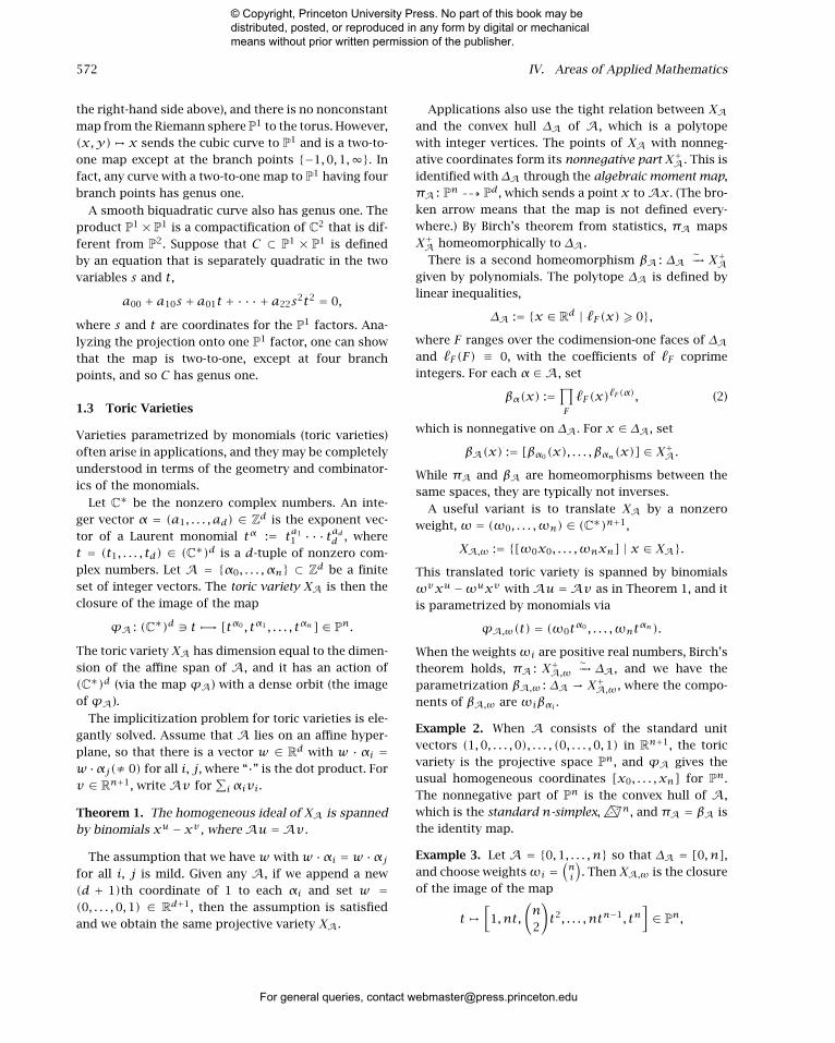
the right-hand side above), and there is no nonconstantmap from the Riemann sphere P1 to the torus. However,(x,y) → x sends the cubic curve to P1 and is a two-to-one map except at the branch points {−1,0,1,∞}. Infact, any curve with a two-to-one map to P1 having fourbranch points has genus one.

A smooth biquadratic curve also has genus one. Theproduct P1 × P1 is a compactification of C2 that is dif-ferent from P2. Suppose that C ⊂ P1 × P1 is definedby an equation that is separately quadratic in the twovariables s and t,

a00 + a10s + a01t + · · · + a22s2t2 = 0,

where s and t are coordinates for the P1 factors. Ana-lyzing the projection onto one P1 factor, one can showthat the map is two-to-one, except at four branchpoints, and so C has genus one.

1.3 Toric Varieties

Varieties parametrized by monomials (toric varieties)often arise in applications, and they may be completelyunderstood in terms of the geometry and combinator-ics of the monomials.

Let C∗ be the nonzero complex numbers. An inte-ger vector α = (a1, . . . , ad) ∈ Zd is the exponent vec-tor of a Laurent monomial tα := ta1

1 · · · tadd , wheret = (t1, . . . , td) ∈ (C∗)d is a d-tuple of nonzero com-plex numbers. Let A = {α0, . . . , αn} ⊂ Zd be a finiteset of integer vectors. The toric variety XA is then theclosure of the image of the map

ϕA : (C∗)d / t −→ [tα0 , tα1 , . . . , tαn] ∈ Pn.

The toric variety XA has dimension equal to the dimen-sion of the affine span of A, and it has an action of(C∗)d (via the map ϕA) with a dense orbit (the imageof ϕA).

The implicitization problem for toric varieties is ele-gantly solved. Assume that A lies on an affine hyper-plane, so that there is a vector w ∈ Rd with w · αi =w ·αj(≠ 0) for all i, j, where “·” is the dot product. Forv ∈ Rn+1, write Av for

∑i αivi.

Theorem 1. The homogeneous ideal of XA is spannedby binomials xu − xv , where Au = Av .

The assumption that we have w with w ·αi = w ·αjfor all i, j is mild. Given any A, if we append a new(d + 1)th coordinate of 1 to each αi and set w =(0, . . . ,0,1) ∈ Rd+1, then the assumption is satisfiedand we obtain the same projective variety XA.

Applications also use the tight relation between XAand the convex hull ΔA of A, which is a polytopewith integer vertices. The points of XA with nonneg-ative coordinates form its nonnegative part X+

A. This isidentified with ΔA through the algebraic moment map,πA : Pn �� Pd, which sends a point x to Ax. (The bro-ken arrow means that the map is not defined every-where.) By Birch’s theorem from statistics, πA mapsX+

A homeomorphically to ΔA.

There is a second homeomorphism βA : ΔA∼−→ X+

Agiven by polynomials. The polytope ΔA is defined bylinear inequalities,

ΔA := {x ∈ Rd | -F(x) � 0},where F ranges over the codimension-one faces of ΔAand -F(F) ≡ 0, with the coefficients of -F coprimeintegers. For each α ∈ A, set

βα(x) :=∏F-F (x)-F (α), (2)

which is nonnegative on ΔA. For x ∈ ΔA, set

βA(x) := [βα0(x), . . . , βαn(x)] ∈ X+A.

While πA and βA are homeomorphisms between thesame spaces, they are typically not inverses.

A useful variant is to translate XA by a nonzeroweight, ω = (ω0, . . . ,ωn) ∈ (C∗)n+1,

XA,ω := {[ω0x0, . . . ,ωnxn] | x ∈ XA}.This translated toric variety is spanned by binomialsωvxu −ωuxv with Au = Av as in Theorem 1, and itis parametrized by monomials via

ϕA,ω(t) = (ω0tα0 , . . . ,ωntαn).

When the weightsωi are positive real numbers, Birch’stheorem holds, πA : X+

A,ω∼−→ ΔA, and we have the

parametrization βA,ω : ΔA → X+A,ω, where the compo-

nents of βA,ω are ωiβαi .

Example 2. When A consists of the standard unitvectors (1,0, . . . ,0), . . . , (0, . . . ,0,1) in Rn+1, the toricvariety is the projective space Pn, and ϕA gives theusual homogeneous coordinates [x0, . . . , xn] for Pn.The nonnegative part of Pn is the convex hull of A,which is the standard n-simplex, n, and πA = βA isthe identity map.

Example 3. Let A = {0,1, . . . , n} so that ΔA = [0, n],and choose weightsωi =

(ni

). Then XA,ω is the closure

of the image of the map

t →[

1, nt,(n2

)t2, . . . , ntn−1, tn

]∈ Pn,




which is the (translated) moment curve. Its nonnegative

part X+A,ω is the image of [0, n] under the map βA,ω

whose components are

βi(x) =1nn

(ni

)xi(n− x)n−i.

Replacing x by ny gives the Bernstein polynomial

βi,n(y) =(ni

)yi(1 −y)n−i, (3)

and thus the moment curve is parametrized by the

Bernstein polynomials. Because of this, we call the

functions ωiβαi (2) generalized Bernstein polynomials.

The composition πA ◦ βA,ω(x) is

1nn

n∑i=0

i(ni

)xi(n− x)n−i

= nxnn

n∑i=1

(n− 1i− 1

)xi−1(n− x)n−i = x,

as the last sum is (x+(n−x))n−1. Similarly, (1/n)πA◦β(y) = y , where β is the parametrization by the Bern-

stein polynomials. The weightsωi =(ni

)are essentially

the unique weights for which πA ◦ βA,ω(x) = x.

Example 4. For positive integers m, n consider the

map ϕ : Cm × Cn → P(Cm×n) defined by

(x,y) → [xiyj | i = 1, . . . ,m, j = 1, . . . , n].

Its image is the Segre variety, which is a toric variety,

as the map ϕ is ϕA, where A is

{ei + fj | i = 1, . . . ,m, j = 1, . . . , n} ⊂ Zm ⊕ Zn.

Here, {ei} and {fj} are the standard bases for Zm and

Zn, respectively.

If zij are the coordinates of Cm×n, then the Segre

variety is defined by the binomial equations

zijzkl − zilzkj =∣∣∣∣∣zij zilzkj zkl

∣∣∣∣∣ .Identifying Cm×n with m × n matrices shows that the

Segre variety is the set of rank-one matrices.

Other common toric varieties include the Veronese

variety, where A is An,d := n d ∩ Zd+1, and the

Segre–Veronese variety, where A is Am,d×An,e. When

d = e = 1, A consists of the integer vectors in them×nrectangle

A = {(i, j) | 0 � i �m, 0 � j � n}.

2 Algorithms for Algebraic Geometry

Mediating between theory and examples and facilitat-ing applications are algorithms developed to study,manipulate, and compute algebraic varieties. Thesecome in two types: exact symbolic methods and approx-imate numerical methods.

2.1 Symbolic Algorithms

The words algebra and algorithm share an Arabic root,but they are connected by more than just their his-tory. When we write a polynomial—as a sum of mono-mials, say, or as an expression such as a determi-nant of polynomials—that symbolic representation isan algorithm for evaluating the polynomial.

Expressions for polynomials lend themselves to algo-rithmic manipulation. While these representations andmanipulations have their origin in antiquity, and meth-ods such as Gröbner bases predate the computer age,the rise of computers has elevated symbolic compu-tation to a key tool for algebraic geometry and itsapplications.

Euclid’s algorithm, Gaussian elimination, and Sylves-ter’s resultants are important symbolic algorithms thatare supplemented by universal symbolic algorithmsbased on Gröbner bases. They begin with a term order≺, which is a well-ordering of all monomials that isconsistent with multiplication. For example, ≺ couldbe the lexicographic order in which xu ≺ xv if thefirst nonzero entry of the vector v −u is positive. Aterm order organizes the algorithmic representationand manipulation of polynomials, and it is the basisfor the termination of algorithms.

The initial term in≺f of a polynomial f is its termcαxα with the ≺-largest monomial in f . The initialideal in≺I of an ideal I is the ideal generated by ini-tial terms of polynomials in I. This monomial ideal is awell-understood combinatorial object, and the passageto an initial ideal preserves much information about Iand its variety.

A Gröbner basis for I is a finite set G ⊂ I of poly-nomials whose initial terms generate in≺I. This set Ggenerates I and facilitates the transfer of informationfrom in≺I back to I. This information may typicallybe extracted using linear algebra, so a Gröbner basisessentially contains all the information about I and itsvariety.

Consequently, a bottleneck in this approach to sym-bolic computation is the computation of a Gröbnerbasis (which has high complexity due in part to its




information content). Gröbner basis calculation also

appears to be essentially serial; no efficient parallel

algorithm is known.

The subject began in 1965 when Buchberger gave

an algorithm to compute a Gröbner basis. Decades of

development, including sophisticated heuristics and

completely new algorithms, have led to reasonably effi-

cient implementations of Gröbner basis computation.

Many algorithms have been devised and implemented

to use a Gröbner basis to study a variety. All of this

is embedded in freely available software packages that

are revolutionizing the practice of algebraic geometry

and its applications.

2.2 Numerical Algebraic Geometry

While symbolic algorithms lie on the algebraic side

of algebraic geometry, numerical algorithms, which

compute and manipulate points on varieties, have a

strongly geometric flavor.

These numerical algorithms rest upon Newton’s

method for refining an approximate solution to a sys-

tem of polynomial equations. A system F = (f1, . . . , fn)of polynomials in n variables is a map F : Cn →Cn with solutions F−1(0). We focus on systems with

finitely many solutions. A Newton iteration is the map

NF : Cn → Cn, where

NF(x) = x −DF−1x (F(x)),

with DFx the Jacobian matrix of partial derivatives of

F at x. If ξ ∈ F−1(0) is a solution to F with DFξ invert-

ible, then when x is sufficiently close to ξ, NF(x) is

closer still, in that it has twice as many digits in com-

mon with ξ as does x. Smale showed that “sufficiently

close” may be decided algorithmically, which can allow

the certification of output from numerical algorithms.

Newton iterations are used in numerical continu-

ation. For a polynomial system Ht depending on a

parameter t, the solutions H−1t (0) for t ∈ [0,1] form a

collection of arcs. Given a point (xt, t) of some arc and

a step δt , a predictor is called to give a point (x′, t+δt)that is near to the same arc. Newton iterations are then

used to refine this to a point (xt+δt , t + δt) on the arc.

This numerical continuation algorithm can be used to

trace arcs from t = 0 to t = 1.

We may use continuation to find all solutions to a sys-

tem F consisting of polynomials fi of degree d. Define

a new system Ht = (h1, . . . , hn) by

hi := tfi + (1 − t)(xdi − 1).

At t = 0, this is xdi − 1, whose solutions are the dthroots of unity. When F is general, H−1

t (0) consists ofdn arcs connecting these known solutions at t = 0 tothe solutions of F−1(0) at t = 1. These may be foundby continuation.

While this Bézout homotopy illustrates the basic idea,it has exponential complexity and may not be efficient.In practice, other more elegant and efficient homotopyalgorithms are used for numerically solving systems ofpolynomials.

These numerical methods underlie numerical alge-braic geometry, which uses them to manipulate andstudy algebraic varieties on a computer. The subjectbegan when Sommese, Verschelde, and Wampler intro-duced its fundamental data structure of a witnessset, as well as algorithms to generate and manipulatewitness sets.

Suppose we have a variety V ⊂ Cn of dimensionn − d that is a component of the zero set F−1(0) ofd polynomials F = (f1, . . . , fd). A witness set for V con-sists of a general affine subspace L ⊂ Cn of dimen-sion d (given by d affine equations) and (approxima-tions to) the points of V ∩ L. The points of V ∩ L maybe numerically continued as L moves to sample pointsfrom V .

An advantage of numerical algebraic geometry is thatpath tracking is inherently parallelizable, as each of thearcs inH−1

t (0)may be tracked independently. This par-allelism is one reason why numerical algebraic geom-etry does not face the complexity affecting symbolicmethods. Another reason is that by computing approx-imate solutions to equations, complete informationabout a variety is never computed.

3 Algebraic Geometry in Applications

We illustrate some of the many ways in which algebraicgeometry arises in applications.

3.1 Kinematics

Kinematics is concerned with motions of linkages (rigidbodies connected by movable joints). While its originswere in the simple machines of antiquity, its impor-tance grew with the age of steam and today it is fun-damental to robotics [VI.14]. As the positions of alinkage are solutions to a system of polynomial equa-tions, kinematics has long been an area of applicationof algebraic geometry.

An early challenge important to the development ofthe steam engine was to find a linkage with a motion




along a straight line. Watt discovered a linkage in 1784

that approximated straight line motion (tracing a curve

near a flex), and in 1864 Peaucellier gave the first link-

age with a true straight line motion (based on circle

inversion):

B

P

(When the bar B is rotated about its anchor point, the

point P traces a straight line.)

Cayley, Chebyshev, Darboux, Roberts, and others

made contributions to kinematics in the nineteenth

century. The French Academy of Sciences recognized

the importance of kinematics, posing the problem of

determining the nontrivial mechanisms with a motion

constrained to lie on a sphere for its 1904 Prix Vaillant,

which was awarded to Borel and Bricard for their partial

solutions.

The four-bar linkage consists of four bars in the plane

connected by rotational joints, with one bar fixed. A

triangle is erected on the coupler bar opposite the fixed

bar, and we wish to describe the coupler curve traced

by the apex of the triangle:

C

B

B'

To understand the motion of this linkage, note that if

we remove the coupler bar C, the bars B and B′ swing

freely, tracing two circles, each of which we parame-

terize by P1 as in (1). The coupler bar constrains the

endpoints of bars B and B′ to lie a fixed distance apart.

In the parameters s, t of the circles and if b, b′, care the lengths of the corresponding bars, the coupler

constraint gives the equation

c2 =(b

1 − s2

1 + s2− b′ 1 − t2

1 + t2)2

+(b

2s1 + s2

− b′ 2t1 + t2

)2

= b2 + b′2 − 2bb′(1 − s2)(1 − t2)+ 4st(1 + s2)(1 + t2) .

Clearing denominators gives a biquadratic equation inthe variety P1 × P1 that parametrizes the rotations ofbars B and B′. The coupler curve is therefore a genus-one curve and is irrational. The real points of a genus-one curve have either one or two components, whichcorresponds to the linkage having one or two assemblymodes; to reach all points of a coupler curve with twocomponents requires disassembly of the mechanism.

Roberts and Chebyshev discovered that there arethree linkages (called Roberts cognates) with the samecoupler curve, and they may be constructed from oneanother using straightedge and compass. The nine-point path synthesis problem asks for the four-bar link-ages whose coupler curve contains nine given points.Morgan, Sommese, and Wampler used numerical con-tinuation to solve the equations, finding 4326 distinctlinkages in 1442 triplets of Roberts cognates. Here isone linkage that solves this problem for the indicatednine points:

Such applications in kinematics drove the early devel-opment of numerical algebraic geometry.

3.2 Geometric Modeling

Geometric modeling uses curves and surfaces to repre-sent objects on a computer for use in industrial design,manufacture, architecture, and entertainment. Theseapplications of computer-aided geometric design andcomputer graphics are profoundly important to theworld economy.

Geometric modeling began around 1960 in the workof de Casteljau at Citroën, who introduced what arenow called Bézier curves (they were popularized byBézier at Renault) for use in automobile manufacturing.

Bézier curves (along with their higher-dimensionalanalogues rectangular tensor-product and triangular




Bézier patches) are parametric curves (and surfaces)that have become widely used for many reasons, includ-ing ease of computation and the intuitive method tocontrol shape by manipulating control points. Theybegin with Bernstein polynomials (3), which are non-negative on [0,1]. Expanding 1n = (t+ (1− t))n showsthat

1 =n∑i=1

βi,n(t).

Given control points b0, . . . ,bn in R2 (or R3), we havethe Bézier curve

[0,1] / t −→n∑i=0

biβi,n(t). (4)

Here are two cubic (n = 3) Bézier curves in R2:

b 0

b 1b 2

b 3 b 0

b 2b 1

b 3

By (4), a Bézier curve is the image of the nonnega-tive part of the translated moment curve of example 3under the map defined on projective space by

[x0, . . . , xn] →n∑i=0

xibi.

On the standard simplex n, this is the canonical mapto the convex hull of the control points.

The tensor product patch of bidegree (m,n) hasbasis functions

βi,m(s)βj,m(t)

for i = 0, . . . ,m and j = 0, . . . , n. These are functionson the unit square. Control points

{bi,j | i = 0, . . . ,m, j = 0, . . . , n} ⊂ R3

determine the map

(s, t) −→∑bijβi,m(s)βj,n(t),

whose image is a rectangular patch.

Bézier triangular patches of degree d have basisfunctions

βi,j;d(s, t) =d!

i!j!(d− i− j)! sitj(1 − s − t)d−i−j

for 0 � i, j with i + j � d. Again, control points givea map from the triangle with image a Bézier triangularpatch. Here are two surface patches:

These patches correspond to toric varieties, with ten-sor product patches coming from Segre–Veronese sur-faces and Bézier triangles from Veronese surfaces. Thebasis functions are the generalized Bernstein polyno-mials ωiβαi of section 1.3, and this explains theirshape as they are images of ΔA, which is a rectanglefor the Segre–Veronese surfaces and a triangle for theVeronese surfaces.

An important question is to determine the intersec-tion of two patches given parametrically as F(x) andG(x) for x in some domain (a triangle or rectangle).This is used for trimming the patches or drawing theintersection curve. A common approach is to solve theimplicitization problem for G, giving a polynomial gwhich vanishes on the patch G. Then g(F(x)) definesthe intersection in the domain of F . This applicationhas led to theoretical and practical advances in algebraconcerning resultants and syzygies.

3.3 Algebraic Statistics

Algebraic statistics applies tools from algebraic geom-etry to questions of statistical inference. This is possi-ble because many statistical models are (part of) alge-braic varieties, or they have significant algebraic orgeometric structures.

Suppose that X is a discrete random variable withn+ 1 possible states, 0, . . . , n (e.g., the number of tailsobserved in n coin flips). If pi is the probability that Xtakes value i,

pi := P(X = i),then p0, . . . , pn are nonnegative and sum to 1. Thus plies in the standardn-simplex, n. Here are two viewsof it when n = 2:

p 0

p 1

p 2 p 0

p 1

p 2

A statistical model M is a subset of n. If the point(p0, . . . , pn) ∈ M , then we may think of X as beingexplained by M .




Example 5. Let X be a discrete random variable whosestates are the number of tails in n flips of a coin with aprobability t of landing on tails and 1 − t of heads. Wemay calculate that

P(X = i) =(ni

)ti(1 − t)n−i,

which is the Bernstein polynomial βi,n (3) evaluated atthe parameter t. We call X a binomial random variableor binomial distribution. The set of binomial distribu-tions as t varies gives the translated moment curve ofexample 3 parametrized by Bernstein polynomials. Thiscurve is the model for binomial distributions. Here is apicture of this curve when n = 2:

p 0

p 1

p 2

Example 6. Suppose that we have discrete randomvariables X and Y with m and n states, respectively.Their joint distribution hasmn states (cells in a table ora matrix) and lies in the simplex mn−1. The model ofindependence consists of all distributions p ∈ mn−1

such that

P(X = i, Y = j) = P(X = i)P(Y = j). (5)

It is parametrized by m−1 × n−1 (probability sim-plices for X and Y ), and (5) shows that it is the nonneg-ative part of the Segre variety of example 4. The modelof independence therefore consists of those joint prob-ability distributions that are rank-one matrices.

Other common statistical models called discreteexponential families or toric models are also the non-negative part X+

A,ω of some toric variety. For these, thealgebraic moment map πA : n → ΔA (or u → Au) isa sufficient statistic. For the model of independence, Auis the vector of row and column sums of the table u.

Suppose that we have data from N independentobservations (or draws), each from the same distribu-tion p(t) from a model M , and we wish to estimate theparameter t best explaining the data. One method is tomaximize the likelihood (the probability of observingthe data given a parameter t). Suppose that the data arerepresented by a vector u of counts, where ui is howoften state iwas observed in theN trials. The likelihoodfunction is

L(t|u) =(Nu

) n∏i=0

pi(t)ui ,

where(Nu

)is the multinomial coefficient.

Suppose thatM is the binomial distribution of exam-

ple 5. It suffices to maximize the logarithm of L(t | u),which is

C +n∑i=0

ui(i log t + (n− i) log(1 − t)),

where C is a constant. By calculus, we have

0 = 1t

n∑i=0

iui +1

1 − tn∑i=0

(n− i)ui.

Solving, we obtain that

t := 1n

n∑i=0

iuiN

(6)

maximizes the likelihood. If u := (u/N) ∈ n is the

point corresponding to our data, then (6) is the nor-

malized algebraic moment map (1/n)πA of example 3

applied to u. For a general toric model X+A,ω ⊂ n,

and likelihood is maximized at the parameter t satisfy-

ing πA◦βA,ω(t) = πA(u). An algebraic formula exists

for the parameter that maximizes likelihood exactly

when πA and βA,ω are inverses.

Suppose that we have data u as a vector of counts

as before and a model M ⊂ n and we wish to test

the null hypothesis that the data u come from a dis-

tribution in M . Fisher’s exact test uses a score functionn → R� that is zero exactly on M and computes

how likely it is for data v to have a higher score than

u, when v is generated from the same probability dis-

tribution as u. This requires that we sample from the

probability distribution of such v .

For a toric model X+A,ω, this is a probability distribu-

tion on the set of possible data with the same sufficient

statistics:

Fu := {v | Au = Av}.

For a parameter t, this distribution is

L(v | v ∈ Fu, t) =(Nv

)ωvtAv∑

w∈Fu(Nw

)ωwtAw

=(Nv

)ωv∑

w∈Fu(Nw

)ωw

, (7)

as Av = Aw for v,w ∈ F(u).This sampling may be accomplished using a random

walk on the fiber Fu with stationary distribution (7).

This requires a connected graph on Fu. Remarkably,

any Gröbner basis for the ideal of the toric variety XAgives such a graph.




3.4 Tensor Rank

The fundamental invariant of an m × n matrix is itsrank. The set of all matrices of rank at most r is definedby the vanishing of the determinants of all (r + 1) ×(r+1) submatrices. From this perspective, the simplestmatrices are those of rank one, and the rank of a matrixA is the minimal number of rank-one matrices that sumto A.

An m × n matrix A is a linear map V2 = Cn → V1 =Cm. If it has rank one, it is the composition

V2v2− C

v1↪−→ V1

of a linear function v2 on V2 (v2 ∈ V∗2 ) and an inclusion

given by 1 → v1 ∈ V1. Thus, A = v1 ⊗ v2 ∈ V1 ⊗ V∗2 , as

this tensor space is naturally the space of linear mapsV2 → V1. A tensor of the form v1 ⊗ v2 has rank one,and the set of rank-one tensors forms the Segre varietyof example 4.

singular value decomposition [II.32] writes amatrix A as a sum of rank-one matrices of the form

A =rank(A)∑i=1

σiv1,i ⊗ v2,i, (8)

where {v1,i} and {v2,i} are orthonormal and σ1 �· · · � σrank(A) > 0 are the singular values of A. Often,only the relatively few terms of (8) with largest singu-lar values are significant, and the rest are noise. LettingAlr be the sum of terms with large singular values andAnoise be the sum of the rest, then A is the sum of thelow-rank matrix Alr plus noise Anoise.

A k-way tensor (k-way table) is an element of thetensor space V1 ⊗ · · · ⊗ Vk, where each Vi is a finite-dimensional vector space. A rank-one tensor has theform v1 ⊗ · · · ⊗ vk, where vi ∈ Vi. These form atoric variety, and the rank of a tensor v is the minimalnumber of rank-one tensors that sum to v .

The (closure of) the set of rank-r tensors is the r thsecant variety. When k = 2 (matrices), the set of deter-minants of all (r + 1)× (r + 1) submatrices solves theimplicitization problem for the r th secant variety. Fork > 2 there is not yet a solution to the implicitizationproblem for the r th secant variety.

Tensors are more complicated than matrices. Sometensors of rank greater than r lie in the r th secant vari-ety, and these may be approximated by low-rank (rank-r ) tensors. Algorithms for tensor decomposition gener-alize singular value decomposition. Their goal is oftenan expression of the form v = vlr + vnoise for a tensorv as the sum of a low-rank tensor vlr plus noise vnoise.

Some mixture models in algebraic statistics aresecant varieties. Consider an inhomogeneous popula-tion in which the fraction θi obeys a probability dis-tribution p(i) from a model M . The distribution ofdata collected from this population then behaves in thesame was as the convex combination

θ1p(1) + θ2p(2) + · · · + θrp(r),which is a point on the r th secant variety of M .

Theoretical and practical problems in complexitymay be reduced to knowing the rank of specific tensors.Matrix multiplication gives a nice example of this.

Let A = (aij) and B = (bij) be 2 × 2 matrices. In theusual multiplication algorithm, C = AB is

cij = ai1b1j + ai2b2j , i, j = 1,2. (9)

This involves eight multiplications. For n×nmatrices,the algorithm uses n3 multiplications.

Strassen discovered an alternative that requires onlyseven multiplications (see the formulas in algorithms

[I.4 §4]). IfA and B are 2k×2kmatrices with k×k blocksaij and bij , then these formulas apply and enable thecomputation of AB using 7k3 multiplications. Recur-sive application of this idea enables the multiplicationof n×n matrices using only nlog2 7 � n2.81 multiplica-tions. This method is used in practice to multiply largematrices.

We interpret Strassen’s algorithm in terms of ten-sor rank. The formula (9) for C = AB is a tensorμ ∈ V ⊗ V∗ ⊗ V∗, where V = M2×2(C). Each multi-plication is a rank-one tensor, and (9) exhibits μ as asum of eight rank-one tensors, so μ has rank at mosteight. Strassen’s algorithm shows that μ has rank atmost seven. We now know that the rank of any ten-sor in V ⊗ V∗ ⊗ V∗ is at most seven, which shows howStrassen’s algorithm could have been anticipated.

The fundamental open question about the complex-ity of multiplying n × n matrices is to determine therank rn of the multiplication tensor. Currently, wehave bounds only for rn: we know that rn � o(n2),as matrices have n2 entries, and improvements tothe idea behind Strassen’s algorithm show that rn <O(n2.3728639).

3.5 The Hardy–Weinberg Equilibrium

We close with a simple application to Mendelian genet-ics.

Suppose that a gene exists in a population in twovariants (alleles) a and b. Individuals will have one



IV.40. General Relativity and Cosmology 579

of three genotypes, aa, ab, or bb, and their distribu-tion p = (paa,pab,pbb) is a point in the probability2-simplex. A fundamental and originally controversialquestion in the early days of Mendelian genetics was thefollowing: which distributions are possible in a popu-lation at equilibrium? (Assuming no evolutionary pres-sures, equidistribution of the alleles among the sexes,etc.)

The proportions qa and qb of alleles a and b in thepopulation are

qa = paa + 12pab, qb = 1

2pab + pbb, (10)

and the assumption of equilibrium is equivalent to

paa = q2a, pab = 2qaqb, pbb = q2

b. (11)

If

A =(

2 1 0

0 1 2

),

with (2

0

)↔ aa,

(1

1

)↔ ab, and

(0

2

)↔ bb,

then (10) is (qa, qb) = 12πA(paa,pab,pbb), the nor-

malized algebraic moment map of examples 3 and 5applied to (paa,pab,pbb). Similarly, the assignmentq → p of (11) is the parametrization β of the trans-lated quadratic moment curve of example 3 given bythe Bernstein polynomials.

Since 12πA◦β(q) = q, the population is at equilibrium

if and only if the distribution (paa,pab,pbb) of alleleslies on the translated quadratic moment curve, that is,if and only if it is a point in the binomial distribution,which we reproduce here:

p 0

p 1

p 2

This is called the Hardy–Weinberg equilibrium after itstwo independent discoverers.

The Hardy in question is the great English mathe-matician G. H. Hardy, who was known for his disdainfor applied mathematics, and this contribution cameearly in his career, in 1908. He was later famous for hiswork in number theory, a subject that he extolled for itspurity and uselessness. As we all now know, Hardy wasmistaken on this last point for number theory underliesour modern digital world, from the security of financialtransactions via cryptography to using error-correcting

codes to ensure the integrity of digitally transmitteddocuments, such as the one you have now finishedreading.

Further Reading

Cox, D., J. Little, and D. O’Shea. 2005. Using AlgebraicGeometry, 2nd edn. Berlin: Springer.

. 2007. Ideals, Varieties, and Algorithms, 3rd edn.Berlin: Springer.

Cox, D., J. Little, and H. Schenck. 2011. Toric Varieties.Providence, RI: American Mathematical Society.

Landsberg, J. M. 2012. Tensors: Geometry and Applications.Providence, RI: American Mathematical Society.

Sommese, A., and C. Wampler. 2005. The Numerical Solutionof Systems of Polynomials. Singapore: World Scientific.

IV.40 General Relativity andCosmologyGeorge F. R. Ellis

General relativity theory is currently the best classi-cal theory of gravity. It introduced a major new themeinto applied mathematics by treating geometry as adynamic variable, determined by the einstein field

equations [III.10] (EFEs). After outlining the basic con-cepts and structure of the theory, I will illustrate itsnature by showing how the EFEs play out in two of itsmain applications: the nature of black holes, and thedynamical and observational properties of cosmology.

1 The Basic Structure: Physics ina Dynamic Space-Time

General relativity extended special relativity (SR) byintroducing two related new concepts.

The first was that space-time could be dynamic. Notonly was it not flat—so consideration of coordinatefreedom became an essential part of the analysis—butit curved in response to the matter that it contained,via the EFEs (6). Consequently, as well as its dynam-ics, the boundary of space-time needs careful consid-eration, along with global causal relations and globaltopology.

Second, gravity is not a force like any other knownforce: it is inextricably entwined with inertia and canbe transformed to zero by a change of reference frame.There is therefore no frame-independent gravitationalforce as such. Rather, its essential nature is encodedin space-time curvature, generating tidal forces andrelative motions.



Documents

IV.39 Algebraic Geometry Frank Sottile - Princeton Universityassets.press.princeton.edu/chapters/s4-39_10592.pdf · algebraic geometry, ... its trove of classical examples, and its