IV Taller Internacional de Analisis no Lineal y EcuacionesDiferenciales Parciales, Manizales, Colombia, Julio 17-20

de 2017

Log-lipschizian Vector Fields in Rn

Marcelo Santoshttp://www.ime.unicamp.br/˜msantosmsantos@ime.unicamp.br • IMECC-UNICAMP, Brazil •Collaborators: Pedro Nel Maluendas Pardo, UPTC, Tunja,Colombia; Edson Jose Teixeira, Federal University of Vicosa,Brazil

Outline

1. Introduction (Motivation)2. Log-lipschizian Vector Fields3. “Picard Theorem” (Cauchy-Lipschitz theorem)4. Osgood Lemma5. Application to compressible fluids

1. INTRODUCTION (MOTIVATION)

Let Ω denote an open set in Rn and I, an open interval in R. Aswe know, a vector fied v in Ω (i.e. a map v : Ω→ Rn) is said to

be lipschitzian when there is a constant C such that

|v(x1)− v(x2)| ≤ C|x1 − x2| (1)

for all x1, x2 ∈ Ω. If the field v is bounded then this condition isequivalent to

sup0 < |x1 − x2| ≤ 1

x1, x2 ∈ Ω

|v(x1)− v(x2)||x1 − x2|

<∞.

Particle trajectory

If the field v depends also on a real variable t ∈ I (physically,this second variable denotes time), the

Picard theorem says that if v = v(x , t) : Ω× I → Rn is acontinuous map and lipschitzian with respect to x ∈ Ω,

uniformly with respect to t ∈ I, i.e. if for some constant C,

|v(x1, t)− v(x2, t)| ≤ C|x1 − x2| (2)

for all x1, x2 ∈ Ω and for all t ∈ I, then for any pair(x0, t0) ∈ Ω× I, there exist a unique solution to the problem

x ′ = v(x , t), x(t0) = x0, (3)

where x ′ ≡ ∂x/∂t is defined in some open open intervalI0 ≡ I(x0, t0) ⊂ I.

Particle trajectory cont’d

We shall denote the above solution by X (· ; x0, t0).The map t ∈ I0 7→ X (t ; x0, t0) is said to be an integral curve ofthe field v , passing by the point x0 at the time t0 or, physically

speaking, in fluid dynamics, the particle trajectory/the trajectoryof the particle that at time t0 is at the point x0, if v(x , t)

represents the velocity of a fluid particle that at time t is at thepoint x .

The map (t ; x0, t0) 7→ X (t ; x0, t0) is called the the flux of the fieldv .

Remark: If v is bounded, then I0 = I, for all (x0, t0) ∈ Ω× I.

Definition

When for all (x0, t0) ∈ Ω× I, the problem

x ′ = v(x , t), x(t0) = x0,

has one and only one solution X (· ; x0, t0), defined is someopen interval I0, we say that the vector field v has a lagrangian

structure.

First example

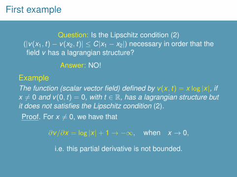
Question: Is the Lipschitz condition (2)(|v(x1, t)− v(x2, t)| ≤ C|x1 − x2|) necessary in order that thefield v has a lagrangian structure?

Answer: NO!

ExampleThe function (scalar vector field) defined by v(x , t) = x log |x |, ifx 6= 0 and v(0, t) = 0, with t ∈ R, has a lagrangian structure butit does not satisfies the Lipschitz condition (2).Proof. For x 6= 0, we have that

∂v/∂x = log |x |+ 1→ −∞, when x → 0,

i.e. this partial derivative is not bounded.

Note

The Lipschitzian condition (2) (|v(x1, t)− v(x2, t)| ≤ C|x1 − x2|)implies that

|∇xv(x , t)| ≤ C

for every point (x , t) where this derivative exists. In fact, for whoknows Measure Theory and Weak Derivatives, we can say thatthe condition (2) is equivalent to the following conditions: thereexists the partial derivatives ∂v/∂xi , as weak derivatives, they

belong to the space L∞(Ω) and ‖∇xv(·, t)‖L∞(Ω) ≤ C for allt ∈ I. This statement is the Rademacher theorem. See e.g. the

book Partial Differential Equations, by Lawrence C. Evans.

The (scalar) field v(x , t) = x log |x | has a lagrangianstructure, i.e.

the problem

x ′ = x log |x |, x(t0) = x0

has a unique solution.Proof. For x0 6= 0, this is a consequence of Picard theorem. Infact, we can compute this solution explicitly by separation of

variables, which is (Exercise/Home Work!):

X (t ; x0, t0) = (sgnx0)|x0|e(t−t0)

,

where sgnx0 = 1 if x0 > 0 and sgnx0 = −1 if x0 < 0.

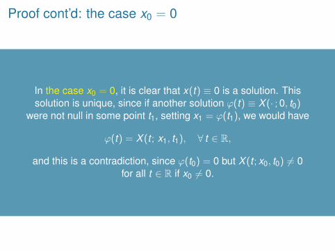
Proof cont’d: the case x0 = 0

In the case x0 = 0, it is clear that x(t) ≡ 0 is a solution. Thissolution is unique, since if another solution ϕ(t) ≡ X (· ; 0, t0)

were not null in some point t1, setting x1 = ϕ(t1), we would have

ϕ(t) = X (t ; x1, t1), ∀ t ∈ R,

and this is a contradiction, since ϕ(t0) = 0 but X (t ; x0, t0) 6= 0for all t ∈ R if x0 6= 0.

Remarks

• There are many non lipschitizian fields with lagrangian structure.Another example is v(x) = 1 + 2x2/3. See Example 1.2.1 in the book

Uniqueness and Nonuniqueness Criteria for Ordinary DifferentialEquations by R. P. Agarwal and V. Lakshmikantham.

• The function −x log x is used in Information Theory to define theso-called Shannon entropy. See the seminal paper Shannon, C. E. A

mathematical theory of communication. Bell System Technical Journal,27 (1948) or Section 4.1 of the book Yockey, Hubert P. Information

theory, evolution, and the origin of life.

• The function x log x is also used in Optimization. See e.g. the worksLopes, Marcos Vinıcius. Trajetoria Central Associada a Entropia e o

Metodo do Ponto Proximal em Programacao Linear. Mastersdissertation - Federal University of Goias, Brazil, 2007. Advisor: Orizon

Pereira Ferreiraand

Ferreira, O. P.; Oliveira, P. R.; Silva, R. C. M. On the convergence of theentropy-exponential penalty trajectories and generalized proximal point

methods in semidefinite optimization. J. Global Optim. 45 (2009).

The field v(x) ≡ v(x , t) = x log |x | satisfies thefollowing property:

|v(x1)− v(x2)| ≤ C|x1 − x2| (1− log |x1 − x2|) (4)(Lipschitz condition modified)

for all x1, x2 ∈ (−1,1) such that 0 < |x1 − x2| ≤ 1.

Notice that − log |x1 − x2| > 0 !

Proof

For x1, x2 ∈ (0,1), assuming x1 < x2, without loss of generality,we have

|v(x1)− v(x2)| = |∫ 1

0dds v (x1 + s(x2 − x1)) ds|

= |(x2 − x1)∫ 1

0 v ′ (x1 + s(x2 − x1)) ds|= |(x2 − x1)

∫ 10 (1 + log(x1 + s(x2 − x1))) ds|

≤ |x2 − x1|(1−∫ 1

0 log(x1 + s(x2 − x1)) ds)

≤ |x2 − x1|(1−∫ 1

0 log s(x2 − x1)ds)

= |x2 − x1|(1−∫ 1

0 (log s + log(x2 − x1)) ds)

= |x2 − x1|(1−∫ 1

0 log s ds −∫ 1

0 log |x2 − x1|ds)= |x2 − x1|(2− log |x2 − x1|) ≤ 2|x2 − x1|(1− log |x2 − x1|)

Proof cont’d

For x1, x2 ∈ (−1,0), we can conclude the same inequality asabove by using that v(x) = x log |x | is an odd function.

Next, let x1 ∈ (−1,0) and x2 ∈ (0,1).If |x1 − x2| = x2 − x1 ≤ e−1 , using that ψ := −x log |x | is

increasing in the interval [−e−1,e−1], we have the followingestimates:

|v(x1)− v(x2)| = x1 log |x1| − x2 log |x2| = ψ(−x1) + ψ(x2)≤ ψ(−x1 + x2) + ψ(x2 − x1) = 2ψ(x2 − x1)= −2(x2 − x1) log(x2 − x1) < 2 (1− (x2 − x1) log(x2 − x1)) .

Proof cont’d

On the other hand, if |x1 − x2| > e−1 , using that v(x) = x log xis bounded in the interval (−1,1), we have

|v(x1)− v(x2)| = |v(x1)−v(x2)||x1−x2| |x1 − x2|

≤ 2(max |v |)e|x1 − x2|≤ 2(max |v |)e|x1 − x2| (1− log |x1 − x2|) .

Finally, we observe that if x1 = 0 or x2 = 0, the condition (4) istrivial, since v(0) = 0.

2

Remark

As we can see from the last argument, to show (4), i.e.|v(x1)− v(x2)| ≤ C|x1 − x2| (1− log |x1 − x2|), it is enough to

consider this inequality for |x1 − x2| less than a certainconstant, since v is bounded.

2. LOG-LIPSCHIZIAN VECTOR FIELDS

Definition

A vector field v in Ω (an open set in Rn) is called log-lipschitzianif it is bounded (for convenience) and satisfies the inequality (4),

i.e.

|v(x1)− v(x2)| ≤ C|x1 − x2| (1− log |x1 − x2|)

for all x1, x2 ∈ Ω such that 0 < |x1 − x2| ≤ 1 i.e.

sup0 < |x1 − x2| ≤ 1

x1, x2 ∈ Ω

|v(x1)− v(x2)||x1 − x2|(1− log |x1 − x2|)

<∞. (5)

Remarks

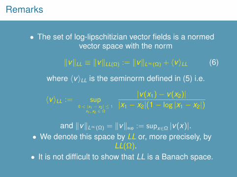
• The set of log-lipschitizian vector fields is a normedvector space with the norm

‖v‖LL ≡ ‖v‖LL(Ω) := ‖v‖L∞(Ω) + 〈v〉LL (6)

where 〈v〉LL is the seminorm defined in (5) i.e.

〈v〉LL := sup0 < |x1 − x2| ≤ 1

x1, x2 ∈ Ω

|v(x1)− v(x2)||x1 − x2|(1− log |x1 − x2|)

and ‖v‖L∞(Ω) = ‖v‖sup := supx∈Ω |v(x)|.• We denote this space by LL or, more precisely, by

LL(Ω).• It is not difficult to show that LL is a Banach space.

3. PICARD THEOREM

Lagrangian structure

The Picard Theorem (Cauchy-Lipschitz theorem) holds forlog-lipschtizian vector fields. More precisely, if v : Ω× I → Rn is

a continuous map such that, for some constant C,

|v(x1, t)− v(x2, t)| ≤ C|x1 − x2|(1− log |x1 − x2|) (7)

for all x1, x2 ∈ Ω with 0 < |x1 − x2| ≤ 1, i.e. ifsupt∈I〈v(·, t)〉LL := sup

0 < |x1 − x2| ≤ 1x1, x2 ∈ Ω

|v(x1)−v(x2)||x1−x2|(1−log |x1−x2|) <∞ then

the field v has a lagrangian structure, i.e. the problemx ′ = v(x , t), x(t0) = x0

has a unique solution X (·; x0, t0), defined in some intervalI0 ≡ I(x0, t0), for all (x0, t0) ∈ Ω× I.

Let us discuss a proof for this theorem.

In the paperChemin, J. Y.; Lerner, N. Flot de champs de vecteurs nonlipschitziens et equations de Navier-Stokes, J. Differential

Equations, 121 (1995), no. 2, 314-328or in the book

Chemin, J. Y. Perfect incompressible fluids. Oxford LectureSeries in Mathematics and its Applications, 14. The Clarendon

Press (1998)we can find a proof which is also valid in infinite dimensional

space, i.e. with Ω being an open set of a Banach space E andv : Ω× I → E as above.

Comparing this proof with the classical proof of Picard theorem,the difference is the way of showing that the Picard iteration is

convergent.

Picard iteration

ϕ0 = x0, ϕk (t) = x0 +

∫ t

t0v(ϕk−1(s), s)ds,

k = 1,2, · · ·Convergence: Let I0 be an open interval such that t0 ∈ I0,

I0 ⊂ I and sufficiently small such that ϕk (t) ∈ Br (x0) ⊂ Ω, forsome closed ball Br (x0) and for all t ∈ I0.

To facilitate the notation, here and in the sequel, we introducethe function

m(r) =

r(1− log r), if 0 < r < 1

r , if r ≥ 1 .(8)

(Notice that we also can write r(1− log r) = r log(1/r).)

Convergence of Picard iteration cont’d

Observe that, for k , l ∈ 1,2, · · · , we have the inequality

|ϕk+l(t)− ϕk (t)| ≤ |∫ t

t0〈v(·, s)〉LLm(|ϕk+l−1(s)− ϕk−1(s)|)ds|,

(9)for t ∈ I0. Then, setting ρk (t) = supl |ϕk+l(t)− ϕk (t)| and using

that m(r) is an increasing function, we obtain

ρk (t) ≤ C|∫ t

t0m(ρk−1(s))ds|, ∀ t ∈ I0.

and, taking the lim sup with respect to k , it follows that

ρ(t) ≤ C|∫ t

t0m(ρ(s))ds| , ∀ t ∈ I0, (10)

where ρ(t) := lim supk ρk (t).

Remark

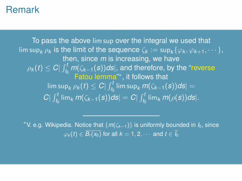
To pass the above lim sup over the integral we used thatlim supk ρk is the limit of the sequence ζk := supkϕk , ϕk+1, · · · ,

then, since m is increasing, we haveρk (t) ≤ C|

∫ tt0

m(ζk−1(s))ds|, and therefore, by the “reverseFatou lemma”∗, it follows that

lim supk ρk (t) ≤ C|∫ t

t0lim supk m(ζk−1(s))ds| =

C|∫ t

t0limk m(ζk−1(s))ds| = C|

∫ tt0

limk m(ρ(s))ds|.

——————————–∗V. e.g. Wikipedia. Notice that m(ζk−1) is uniformly bounded in I0, since

ϕk (t) ∈ Br (x0) for all k = 1, 2, · · · and t ∈ I0

• The inequality (10) implies that ρ is null (next slide).• Let ϕ(t) = limk ϕk (t), t ∈ I0.

• To conclude that ϕ(t) is a solution to the problem (3),we can use the Lebesgue Dominated ConvergenceTheorem and take the limk→∞ in the Picard iteration

ϕk (t) = x0 +∫ t

t0v(ϕk−1(s), s)ds.

4. OSGOOD LEMMA

Osgood lemma

Let γ : R→ R+ := [0,∞) a locally integrable function andω : R+ → R+, continuous non decreasing and such thatω(r) > 0 if r > 0. Assume that a continuous non negativefunction ρ satisfies the inequality

ρ(t) ≤ a +

∫ t

t0γ(s)ω(ρ(s))ds,

for a real number a ≥ 0, t0 ∈ R, and all t ≥ t0 in an interval Jcontaining t0. If a > 0 then

−M(ρ(t)) + M(a) ≤∫ t

t0γ(s)ds, t ∈ J ∩ [t0,∞)

where M(x) :=∫ 1

xdrω(r) , x > 0. If a = 0 and

∫ 10

1ω(r)dr =∞,

then ρ(t) = 0 for all t ∈ J ∩ [t0,∞).

Proof

Letting R(t) = a +∫ t

t0γ(s)ω(ρ(s))ds, t ∈ J ∩ [t0,∞), we have

ρ(t) ≤ R(t) and R′(t) = γ(t)ω(ρ(t)) ≤ γ(t)ω(R(t)), a.e.In the case a > 0, R(t) > 0, then

− ddt

M(R(t)) =1

ω(R(t))R′(t) ≤ γ(t).

Therefore, integrating from t0 to t , we obtain the inequality−M(ρ(t)) + M(a) ≤

∫ tt0γ(s)ds.

In the case a = 0, we have ρ(t) ≤ a′ +∫ t

t0γ(s)ω(ρ(s))ds, for all

a′ > 0, then, by the case a > 0, we obtain

M(a′) ≤∫ t

t0γ(s) ds + M(ρ(t))

for all a′ > 0. Therefore, droping a′ to zero, it follows that∫ 10

1ω(r)dr <∞ if ρ(t) > 0 for some t ∈ J ∩ [t0,∞). 2

Remarks

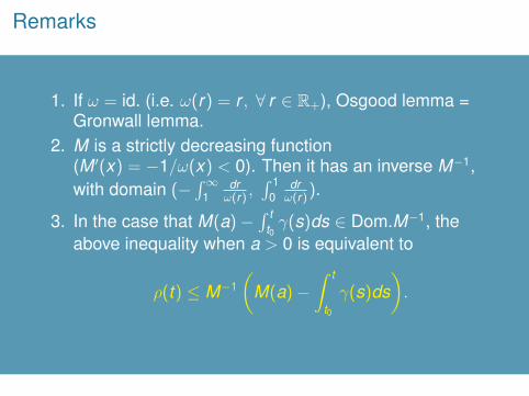
1. If ω = id. (i.e. ω(r) = r , ∀ r ∈ R+), Osgood lemma =Gronwall lemma.

2. M is a strictly decreasing function(M ′(x) = −1/ω(x) < 0). Then it has an inverse M−1,with domain (−

∫∞1

drω(r)

,∫ 1

0drω(r)

).

3. In the case that M(a)−∫ t

t0γ(s)ds ∈ Dom.M−1, the

above inequality when a > 0 is equivalent to

ρ(t) ≤ M−1(

M(a)−∫ t

t0γ(s)ds

).

Remars cont’d

4. For the function ω = m given in (8),

M(x) =

ln(1− ln x), if 0 < x ≤ 1− ln x , if x ≥ 1

M−1(y) =

e−y , if y ≤ 0e(1−exp(y)), if y ≥ 0 .

Then, if M(a)−∫ t

t0γ(s)ds ≥ 0 and a ≤ 1, i.e.

a ≤ min1,e(1−exp(∫ t

t0γ(s)ds)), we have the inequality

ρ(t) ≤ e1−exp(M(a)−∫ t

t0γ(s)ds)

= e1−(1−ln a) exp(−∫ t

t0γ(s)ds)

,

i.e.ρ(t) ≤ aexp(−

∫ tt0γ(s)ds)e1−exp(−

∫ tt0γ(s)ds)

. (11)

Uniqueness of trajectories

Let ψ1 and ψ2 be solutions to the problem (3). Similarly to (9),we have

|ψ1(t)− ψ2(t)| ≤∫ t

t0〈v(·, s)〉LLm(|ψ1(s)− ψ2(s))|)ds,

then by Osgood lemma, it follows that ψ1 = ψ2.

Continuous dependence on the initial point

|X (t ; x1, t0)− X (t ; x2, t0)|≤ |x1 − x2|+

∫ tt0〈v(·, s)〉LLm(|X (s; x1, t0)− X (s; x2, t0)|)ds,

thus, from (11), we have

|X (t ; x1, t0)− X (t ; x2, t0)| ≤ |x1 − x2|exp(−

∫ tt0γ(s)ds)e1−exp(−

∫ tt0γ(s)ds)

,(12)

for 0 < |x1 − x2| ≤ min1,e1−exp(∫ t

t0γ(s)ds), if γ(s) := 〈v(·, s)〉LL

is locally integrable, e.g. if v is uniformly log-lipschitzian, as in(7).

Theorem

The constant C in (7) can be replaced by a locally integrablefunction in t , i.e. a vector field v in Ω× I has a lagrangian

structure if the seminorm 〈v(·, s)〉LL(Ω) is locally integrable in I.More precisely, we have the following theorem:

Let v : Ω× I → Rn be a map in L1loc(I; LL(Ω)). Then, for any

t0 ∈ I, there exists a unique continuous mapX (· ; ·, t0) : I × Ω→ Ω such that

X (t ; x , t0) = x +

∫ t

t0v(X ((s; x , t0), s)ds, (t , x) ∈ I × Ω. (13)

In addition, we have the estimate (12), with γ(s) = 〈v(·, s)〉LL,for any x1, x2 ∈ Ω such that

0 < |x1 − x2| ≤ min1,e1−exp(∫ t

t0γ(s)ds).

Remark

The estimate (12) means that for each t ∈ I, the mapx ∈ Ω 7→ X (t ; x , t0) is Holder continuous, with exponent given

by α = exp(−∫ t

t0〈v(·, s)〉LLds).

2 comments

• The relation between the space of lipschitzianfunctions, log-lipschitzian functions and Holdercontinuous functions:

Lip ⊂ LL ⊂ Cα

• The inclusion LL ⊂ Cα has been used to obtain betterregularity than Cα in problems of free boundaries orfully nonlinear equations, cf. the papersLeitao, Raimundo; de Queiroz, Olivaine S.; Teixeira, Eduardo.Regularity for degenerate two-phase free boundary problems,Ann. l’Inst. H. Poincare (C) Non Linear An., 32 (2015), no. 4,741-762;———–Teixeira, Eduardo. Universal moduli of continuity for solutions tofully nonlinear elliptic equations. Arch. Ration. Mech. Anal. 211(2014), no. 3, 911-927.

An interesting remark

The Sobolev space Hn2 +1(Rn) is immerse in

the space LL(Rn).

AN USEFUL EXAMPLE

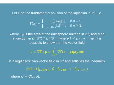
Let Γ be the fundamental solution of the laplacian in Rn, i.e.

Γ(x) =

− 1

2π log |x |, if n = 21

(2−n)ωn|x |2−n, if n ≥ 3,

where ωn is the area of the unit sphere unitaria in Rn, and g bea function in Lp(Rn) ∩ L∞(Rn), where 1 ≤ p < n. Then it is

possible to show that the vector field

v = ∇Γ ∗ g =

∫Rn∇Γ(x − y)g(y)dy

is a log-lipschitzian vector field in Rn and satisfies the inequality

‖∇Γ ∗ f‖LL(Rn) ≤ C(‖f‖Lp(Rn) + ‖f‖L∞(Rn))

where C = C(n,p).

5. APPLICATION TO COMPRESSIBLE FLUIDS

Compressible fluids (Navier-Stokes) equations:

ρt + div(ρv) = 0(ρv j)t + div(ρv jv) + P(ρ)xj = µ∆v j + λ div vxj + ρf j

Solution obtained by David Hoff:

• Hoff, David. Global solutions of the Navier-Stokesequations for multidimensional, compressible flow withdiscontinuous initial data. J. Diff. Eqns. 120, no. 1 (1995),215-254.• Hoff, David. Discontinuous solutions of the Navier-Stokes

equations for multidimensional, heat-conducting flow.Archive Rational Mech. Ana. 139 (1997), 303–354.

• Hoff, David. Compressible Flow in a Half-Space withNavier Boundary Conditions. J. Math. Fluid Mech. 7(2005), 315–338.

Distinguished properties

• P(ρ) ∈ L2(Rn) ∩ L∞(Rn), n = 2,3• The quantities ωj ,k = v j

xk − vkxj

andF = (µ + λ)div v − P(ρ) are Holder

continuous.

Decomposition of the velocity field

∆v j = v jxk xk

= vkxk xj

+ (v jxk− vk

xj)xk

= div vxj + ωj,kxk

= (µ+ λ)−1Fxj + ωj,kxk

+ (µ+ λ)−1P(ρ)xj

(14)

thus, we can write

v = vF ,ω + vP

where

vF ,ω = (µ+ λ)−1∇Γ ∗ F + Γxk ∗ ω·,k

vP = ∇Γ ∗ P(ρ) .

Last slide

• From the ‘‘useful example’’, we can conclude that vP ∈ LL.• Since F and ωj,k are Holder continuous, we can conclude

that vF ,ω ∈ Lip.• Theorem (Hoff- –, ARMA, 2008). 〈v(·, t)〉LL ∈ L1

loc .

Thank you!!