Embed Size (px)
Citation preview

ITS Communications Document
Prepared by:
Lockheed Martin Federal SystemsOdetics Intelligent Transportation Systems Division
Prepared for:
Federal Highway AdministrationUS Department of TransportationWashington, D. C. 20590
January 1997

iii
TABLE OF CONTENTS
National ITS Communication – Executive Summary ...................................................................... ES-1
1. Introduction........................................................................................................................................1-11.1 Purpose of Document..................................................................................................................... 1-11.2 Structure of Document ................................................................................................................... 1-2
2. Introduction to the ITS Communication Architecture ...................................................................2-12.1 Role of the Communication Architecture....................................................................................... 2-12.2 The Telecommunication Infrastructure and the ITS Communication Architecture DevelopmentPhilosophy ........................................................................................................................................... 2-22.3 Development of a Communications Architecture .......................................................................... 2-52.4 Elements of the Communications Layer of the ITS Architecture................................................... 2-52.5 Relationship of the Communication Architecture Definition to the Data Loading Analysis andSimulations .......................................................................................................................................... 2-7
3. Communication Architecture Definition..........................................................................................3-13.1 Communication Architecture ......................................................................................................... 3-4
3.1.1 Communication Services ........................................................................................................................... 3-53.1.2 Logical Communication Functions............................................................................................................ 3-63.1.3 Functional Entities..................................................................................................................................... 3-73.1.4 Communication Network Reference Model............................................................................................... 3-7
3.2 Communication Layer Linkage...................................................................................................... 3-93.2.1 Mapping Communication Services to Data Flows..................................................................................... 3-93.2.2 Architecture Interconnect Diagrams .......................................................................................................... 3-93.2.2.1 AID Template ..................................................................................................................................... 3-103.2.2.2 Level 1 AIDs....................................................................................................................................... 3-113.2.2.3 Level 0 AID ........................................................................................................................................ 3-12
3.2.3 Architecture Renditions ........................................................................................................................... 3-163.2.3.1 Level 1 Rendition ............................................................................................................................... 3-163.2.3.2 Level 0 Rendition ............................................................................................................................... 3-17
3.2.4 Architecture Interconnect Specifications ................................................................................................. 3-18
4. Scenarios and Time Frames ..............................................................................................................4-14.1 Evaluatory Design.......................................................................................................................... 4-14.2 Baseline Information for the Scenario Regions.............................................................................. 4-14.3 Number of Potential Users by User Service Group........................................................................ 4-24.4 Penetrations.................................................................................................................................... 4-34.5 Assignment of Users to Communications Interfaces...................................................................... 4-54.6 Usage Profiles for the User Service Groups................................................................................. 4-134.7 4.7 Scenario Infrastructure Model ............................................................................................... 4-15
5. Message Definition.............................................................................................................................5-15.1 Message Definition Methodology.................................................................................................. 5-25.2 Message Structure.......................................................................................................................... 5-25.3 Message Set ................................................................................................................................... 5-4
6. Data Loading Methodology and Results..........................................................................................6-16.1 Data Loading Models..................................................................................................................... 6-36.2 Wireless Data Loads ...................................................................................................................... 6-3
6.2.1 Two-Way Wireless Data Loads ................................................................................................................. 6-36.2.1.1 Histogram of Message Size Distribution ............................................................................................ 6-30
6.2.2 Broadcast Data Loads .............................................................................................................................. 6-336.2.3 Short Range DSRC Data Loads............................................................................................................... 6-34

iv
6.3 Wireline Data Loads .................................................................................................................... 6-346.4 Analysis of the Data Loading Results .......................................................................................... 6-88
6.4.1 u1t Interface............................................................................................................................................. 6-886.4.2 u1b Interface ............................................................................................................................................ 6-886.4.3 u2 Interface .............................................................................................................................................. 6-896.4.4 u3 Interface .............................................................................................................................................. 6-896.4.5 Wireline Interface .................................................................................................................................... 6-89
7. Assessment of Communication Systems and Technologies.............................................................7-17.1 Introduction.................................................................................................................................... 7-1
7.1.1 Objectives of the Technology Assessment................................................................................................. 7-27.1.2 Underlying Assumptions ........................................................................................................................... 7-27.1.3 Section Structure........................................................................................................................................ 7-2
7.2 Communication Systems Analysis and Assessment Approach ...................................................... 7-57.2.1 Wireless Communication Systems Analysis .............................................................................................. 7-57.2.1.1 Wide-Area Communication Systems .................................................................................................... 7-57.2.1.2 Short-Range Communications.............................................................................................................. 7-5
7.2.2 Wireline Communication Analysis ............................................................................................................ 7-67.2.3 End-to-End Communication Analysis ....................................................................................................... 7-6
7.3 Non-ITS Applications and Their Impact........................................................................................ 7-77.3.1 Non-ITS Wireless Data Market Projections for 2002................................................................................ 7-87.3.2 Characterization of Non-ITS Applications Traffic................................................................................... 7-107.3.2.1 E-Mail Traffic Characterization (12.7 Million Users) ........................................................................ 7-107.3.2.2 Internet Access Traffic Characterization (12.7 Million Users) ........................................................... 7-137.3.2.3 Other Non-ITS Applications............................................................................................................... 7-18
7.4 Protocol and Inter-networking Issues........................................................................................... 7-197.5 Technology Assessment............................................................................................................... 7-20
7.5.1 Wireless Communications ....................................................................................................................... 7-207.5.1.1 Wide-Area versus Short-Range .......................................................................................................... 7-227.5.1.2 Short Range ITS Communications ..................................................................................................... 7-97
7.5.2 Wireline Communications ..................................................................................................................... 7-1017.5.2.1 Candidate Wireline Technologies..................................................................................................... 7-1027.5.2.2 Candidate Wireline Topologies ........................................................................................................ 7-1037.5.2.3 Public Network Usage ...................................................................................................................... 7-1047.5.2.4 Localized Use of Internet.................................................................................................................. 7-105
7.6 Technology Survey and Assessment Summary.......................................................................... 7-114
8. Communication Systems Performance – A Case Study..................................................................8-18.1 Wireless Systems Performance ...................................................................................................... 8-2
8.1.1 Scope of Performance Analysis ................................................................................................................. 8-28.1.1.1 Urbansville 2002 and 2012................................................................................................................... 8-28.1.1.2 Thruville 2002 .................................................................................................................................... 8-138.1.1.3 Mountainville ..................................................................................................................................... 8-14
8.1.2 Simulation Strategy.................................................................................................................................. 8-148.1.3 CDPD Protocol Overhead........................................................................................................................ 8-178.1.4 Non-ITS Applications CDPD Data Loads ............................................................................................... 8-218.1.5 CDPD Data Loads ................................................................................................................................... 8-228.1.5.1 Urbansville ......................................................................................................................................... 8-228.1.5.2 Thruville 2002 .................................................................................................................................... 8-44
8.2 CDPD Simulation Results............................................................................................................ 8-558.2.1 Urbansville 2002 and 2012...................................................................................................................... 8-558.2.1.1 Capacity Comparison of One Reserved CDPD Channel versus One Reserved Plus One DynamicallyAssigned CDPD Channels.............................................................................................................................. 8-578.2.1.2 Urbansville 2012 -- One Reserved CDPD Channel............................................................................ 8-588.2.1.3 Urbansville 2002 -- One Reserved CDPD Channel............................................................................ 8-618.2.1.4 Urbansville 2002 -- Dynamic Assignment of CDPD Channels (No Reserved Channel).................... 8-72
8.2.2 Thruville 2002 ......................................................................................................................................... 8-778.2.3 Mountainville........................................................................................................................................... 8-81
8.3 Wireline System Performance...................................................................................................... 8-83

v
8.3.1 Traffic Over the Wireline Portion of the CDPD Network...................................................................8-838.4 End-to-End System Performance............................................................................................8-86
8.4.1 Scope of Performance Analysis..........................................................................................................8-868.4.2 Results..............................................................................................................................................8-87
9. ITS Architecture Communication – Conclusions....................................................................... 9-1
Communications Document HRI Addendum - January 1997

vi
APPENDICES
Appendix A Communication Architecture Development and Definitions ..................................... A-1A.1 Communication Services Descriptions......................................................................................... A-1
A.1.1 Interactive Services .................................................................................................................................. A-4A.1.2 Distribution Services................................................................................................................................ A-5A.1.3 Location Services..................................................................................................................................... A-5A.1.3.1 Location Determination Techniques ................................................................................................... A-6A.1.3.2 Types of Location Services................................................................................................................. A-6A.1.3.3 Service Deployment Issues ................................................................................................................. A-7
A.2 Logical Communication Function Definitions ............................................................................. A-7A.3 Network Entity Definitions .......................................................................................................... A-8A.4 Network Reference Model ......................................................................................................... A-12A.5 Communication Architecture Linkage........................................................................................ A-14
A.5.1 Mapping Communication Services to Data Flows................................................................................. A-14
Appendix B Architecture Interconnect Diagrams - Level 1 ............................................................ B-1
Appendix C Communication Architecture Renditions and Applicable Technologies .................. C-1C.1 Format/Purpose ............................................................................................................................ C-2
C.1.1 Level 0 Rendition......................................................................................................................................C-2C.1.2 Level 1 Rendition......................................................................................................................................C-3
C.2 Applicable Technologies Mapped to the Renditions.................................................................. C-27
Appendix D Technology Assessment Sources................................................................................... D-1D.1 Wireless ....................................................................................................................................... D-1
D.1.1 MAN’s ..................................................................................................................................................... D-1D.1.2 Land Mobile Systems............................................................................................................................... D-2D.1.3 Satellite Mobile Systems.......................................................................................................................... D-4D.1.4 Meteor Burst Systems .............................................................................................................................. D-5D.1.5 Broadcast Systems ................................................................................................................................... D-5D.1.5.1 FM Subcarrier..................................................................................................................................... D-5D.1.5.2 DAB.................................................................................................................................................... D-5
D.1.6 Short-Range Communications ................................................................................................................. D-5D.1.6.1 DSRC Communications...................................................................................................................... D-5D.1.6.2 Vehicle-to-Vehicle Communications.................................................................................................. D-6
D.2 Wireline Communications............................................................................................................ D-6
Appendix E Potential Users According to User Service Group ...................................................... E-1E.1 Private Vehicle Service Group Users – Urbansville, 1997............................................................E-2E.2 CVO - Long-Haul Service Group Users........................................................................................E-3E.3 CVO - Local Service Group Users ................................................................................................E-3E.4 Traveler Information Service Group Users ...................................................................................E-4E.5 Public Transportation Management Service Users........................................................................E-4E.6 Emergency Response Vehicles Management Services ..................................................................E-4E.7 Probes............................................................................................................................................E-4
Appendix F Message Definitions And Data Loading Models...........................................................F-1
Appendix G Use of Beacons For Wide Area Delivery/Collection Of ITS Information.................G-1G.1 Introduction.................................................................................................................................. G-1G.2 Candidate Beacon Deployment .................................................................................................... G-2G.3 Message Compatibility with DSRC ............................................................................................. G-3G.4 Impact of ITS Data on Beacon Capacity...................................................................................... G-3G.5 Impact of DSRC Traffic on Wireline Network ............................................................................ G-3

vii
G.6 Some Problems with Beacon Systems.......................................................................................... G-6G.7 Summary ...................................................................................................................................... G-9
Appendix H Wireless and Wireline Protocols ..................................................................................H-1H.1 Wireless Protocols ....................................................................................................................... H-1
H.1.1 CDPD....................................................................................................................................................... H-1H.1.2 CDPD Protocols as Implemented in MOSS............................................................................................. H-1H.1.3 GPRS ....................................................................................................................................................... H-5
H.2 Wireline Protocols ....................................................................................................................... H-5H.2.1 Ethernet.................................................................................................................................................... H-5H.2.2 FDDI........................................................................................................................................................ H-6H.2.3 ATM ........................................................................................................................................................ H-6
Appendix I Simulation Tools............................................................................................................... I-1I.1 Introduction .....................................................................................................................................I-1I.2 Wireless Communications (Cellular/PCS).......................................................................................I-3
I.2.1 Graphical RAdio Network Engineering Tool (GRANET)...........................................................................I-4I.2.2 MObile Systems Simulator (MOSS) ...........................................................................................................I-5I.2.3 Integrated GRANET+MOSS.......................................................................................................................I-7
I.3 OPtimized Network Engineering Tools (OPNET) ..........................................................................I-8I.3.1 Wireline Communications...........................................................................................................................I-8I.3.2 Wireless + Wireline Simulation Integration ................................................................................................I-9
I.4 Validation of the Modeling Tools....................................................................................................I-9
Appendix J CDPD Field Trial Results ............................................................................................... J-1J.1 Introduction ................................................................................................................................... J-1J.2 Trial Objectives............................................................................................................................. J-2J.3 Trial Participants ........................................................................................................................... J-2J.4 FleetMaster System and Trial Configuration................................................................................. J-3J.5 Sample Field Results ..................................................................................................................... J-4
J.5.1 Signal Strength and Waiting Time Measurements .....................................................................................J-4J.5.2 TCP versus UDP ........................................................................................................................................J-6J.5.3 CDPD System Loading Limits ...................................................................................................................J-7J.5.4 Application Inter-Arrival Times with UDP................................................................................................J-7
J.6 Operation in Customer’s Vehicles and Billing System Validation Tests..................................... J-10J.7 Summary of Conclusions............................................................................................................. J-11

viii
FIGURES
Figure 2.2-1 Overview of the Telecommunications Arena ................................................................. 2-2Figure 2.4-1 Communication Architecture Development Process ...................................................... 2-6
Figure 3.0–1 Communications Architecture Development Process .................................................... 3-3Figure 3.1-1 Generic Hierarchical Communication Model.................................................................. 3-5Figure 3.1-2 Communication Services Hierarchy ................................................................................ 3-6Figure 3.1.-3 Network Reference Model for the Communications Layer ............................................ 3-8Figure 3.1-4 Implementation Flexibility of ITS Architecture Data Flows .......................................... 3-8Figure 3.2-1. Template for the Architecture Interconnect Diagram (AID) ........................................ 3-11Figure 3.2-2 Example of AID Level-1 ............................................................................................... 3-11Figure 3.2-3 Level 0 Architecture Interconnect Diagram for the National ITS Architecture............ 3-13Figure 3.2-4 Level 0 Architecture Interconnect Diagram for the National ITS Architecture............ 3-14Figure 3.2-5 Level 0 Architecture Interconnect Diagram for the National ITS Architecture;........... 3-15Figure 3.2-6 Rendition 1 — Wide-Area Wireless (u1) Link Through Switched Networks .............. 3-16Figure 3.2-7 Rendition 1 for Wide-Area One-Way Wireless (u1b) Links ....................................... 3-17Figure 3.2-8 Level 0 Rendition ......................................................................................................... 3-18Figure 3.2-9 AIS Example Using CDPD for Wide Area Wireless (u1) ............................................ 3-19
Figure 5.1-1 Level 0 Architecture Interconnect Diagram for the National ITS Architecture.............. 5-1Figure 5.2-1 Examples of Message Structures .................................................................................... 5-2Figure 5.2-2 Details of the Message_ID Field which Allows Standard, Optional,and Repeated Fields to be Appended to the Message .......................................................................... 5-3Figure 5.2-3 Example of an Optional-Field Message.......................................................................... 5-3Figure 5.2-4 Example of a Message with Three Sets of Repeated Fields ........................................... 5-4
Figure 6.2-26 Distribution of Messages per Population, Urban Area, 2002, Peak Period................ 6-32
Figure 7.3-1 2002 Wireless Data Market Projections (from External and GTE Market Studies)..... 7-10Figure 7.3-2 Time-of-Day E-mail Pattern -- Incoming E-mail.......................................................... 7-11Figure 7.3-3 Time-of-Day E-mail Pattern -- Outgoing E-mail ........................................................... 7-11Figure 7.3-4 Histogram of Message Size up to 100 kbytes (Not to Scale)........................................ 7-12Figure 7.3-5 Histogram of Wireless E-mail Message Sizes (up to 5 kbytes) .................................... 7-13Figure 7.3-6 Daily Statistics for the Boston University WWW Server............................................. 7-14Figure 7.3-7 Daily Statistics for the MIT WWW Server .................................................................. 7-15Figure 7.3-8 Weekly Statistics from the Boston University WWW Server ...................................... 7-16Figure 7.3-9 Weekly Statistics from the MIT WWW Server............................................................ 7-17Figure 7.5-1 Metricom’s Present and Planned Coverage in the San Francisco Bay Area................. 7-24Figure 7.5-2 Example of a City-wide Deployment of Metricom’s Ricochet System ........................ 7-25Figure 7.5-3 CDPD Deployment as of the Fourth Quarter of 1995 .................................................. 7-29Figure 7.5-4 CDPD Network Architecture........................................................................................ 7-29(From Wireless Information Networks, K. Pahlavan, A. Levesque, John Wiley & Sons, Inc., 1995.Note: the A interface is referred to in this document as the u1t interface). ....................................... 7-29Figure 7.5-5 CDPD Protocol Stack (CDPD System Specification, Release 1.0).............................. 7-31Figure 7.5-6 CDPD Protocol Stack (CDPD System Specification, Release 1.1)............................... 7-32Figure 7.5-7 Average Delay/Call Duration Ratio: CDPD versus Circuit-Switched CDMA ............. 7-37Figure 7.5-8 Omnipoint’s System Architecture and Public-Private Operation ................................. 7-39Figure 7.5-9 GSM Frame and Slot Structure .................................................................................... 7-41Figure 7.5-10 ARDIS Coverage in the Mid-Atlantic and Southern California Regions ................... 7-44Figure 7.5-11 ARDIS Network Architecture .................................................................................... 7-45Figure 7.5-12 MOBITEX Network Architecture .............................................................................. 7-47Figure 7.5-13 Satellite Orbits............................................................................................................ 7-54

ix
Figure 7.5-14 Location of, and Coverage Provided by, the Two Already Deployed ORBCOMMSatellites at Two Instants in Time...................................................................................................... 7-56Figure 7.5-15 Iridium System Footprint at a Given Point in Time.................................................... 7-59Figure 7.5-16 Path Described by a Teledesic Satellite...................................................................... 7-60Figure 7.5-17 ICO’s Satellite Orbits ................................................................................................. 7-63Figure 7.5-18 SKYCELL Coverage.................................................................................................. 7-64Figure 7.5-19 MSAT North American Coverage.............................................................................. 7-65Figure 7.5-20 VSAT Network Configuration ................................................................................... 7-71Figure 7.5-21 GPS Constellation ...................................................................................................... 7-72Figure 7.5-22 GLONASS Constellation .......................................................................................... 7-73Figure 7.5-23 Motion of Ground Illumination Region due to Trail Formation and Decay ............... 7-74Figure 7.5-24 Effect of Trail Location on Size of Footprint ............................................................. 7-74Figure 7.5-25 FM Spectrum Allocation in North America and Europe ............................................ 7-78Figure 7.5-26 FM Baseband Spectrum (Not to scale)....................................................................... 7-79Figure 7.5-27 Single Group Standard RDS Message........................................................................ 7-80Figure 7.5-28 SCA FM Spectrum ..................................................................................................... 7-82Figure 7.5-29 HSDS Coverage in the Southern California Area forWrist-Watch Receiver (-29 dBi antenna)......................................................................................... 7-83Figure 7.5-30 HSDS Coverage in the Portland, OR, and Seattle, WA, Areas forWrist-Watch Receiver (-29 dBi antenna)........................................................................................... 7-84Figure 7.5-31 FM Baseband Spectrum usage for Seiko’s HSDS System ......................................... 7-85Figure 7.5-32 FM Baseband Spectrum Usage for MITRE’s STIC System....................................... 7-87Figure 7.5-33 FM Baseband Spectrum Usage for NHK’s DARC System ........................................ 7-88Figure 7.5-34 Full Deployment of a Beacon System ........................................................................ 7-94Figure 7.5-35 Dead Zone Crossing Times ........................................................................................ 7-95Figure 7.5-36 Beacon Coverage Crossing Time ............................................................................... 7-96Figure 7.5-37 PDF’s of the Round-Trip Delay ............................................................................... 7-106Figure 7.5-37 PDF’s of the Round-Trip Delay (Cont.) ................................................................... 7-107Figure 7.5-38 Average Round-Trip Delay (Period March 5-7, 1996) ............................................ 7-108Figure 7.5-38 Average Round-Trip Delay (Period March 5-7, 1996) (Cont.) ................................ 7-109Figure 7.5-39 Example of the Range of Round-Trip Delays (Boston, March 5-7, 1996) ............... 7-110Figure 7.5-39 Example of the Range of Round-Trip Delays (Boston, March 5-7, 1996) (Cont’d) 7-111Figure 7.5-40 Minimum-Average-Maximum Packet Loss (Boston, March 5-7, 1996) .................. 7-112Figure 7.5-40 Minimum-Average-Maximum Packet Loss (Boston, March 5-7, 1996) (Cont’d).... 7-113
Figure 8.1-1 Base Station Locations in the Detroit Area .................................................................. 8-11Figure 8.1-2 Best Server Map of the Detroit Area (Obtained Using GRANET) .............................. 8-12Figure 8.1-3 Communication System Simulation/Evaluation Methodology ...................................... 8-15Figure 8.1-4 Quantitative Technical MOE’s...................................................................................... 8-17Figure 8.1-5 CDPD Protocol Stack (Cellular Digital Packet Data System Specification,Release 1.0)........................................................................................................................................ 8-18Figure 8.1-6 Framing and Block Structure Showing the Color Code................................................. 8-20Figure 8.1-7 Histogram of Wireless E-mail Message Sizes (up to 5 kbytes) ..................................... 8-21Figure 8.1-8 Average File Transfer Size for the MIT WWW Server(All day Average: 8490 bytes) ........................................................................................................... 8-22Figure 8.1-9 Location of the Incident showing the Sectors Involved, as well as the Sectors andRoadway Segments Affected by the Incident..................................................................................... 8-43Figure 8.1-10 Extension of the Queues induced by the Incident immediately before its Dissipation,showing the Affected Sectors............................................................................................................. 8-54Figure 8.2-1 Detroit (Urbansville) Coverage ..................................................................................... 8-56Figure 8.2-2 Capacity of a Reserved CDPD Channel ....................................................................... 8-57Figure 8.2-3 Capacity of One Reserved plus One Dynamically Assigned CDPD Channels............. 8-58Figure 8.2-4 Delay/Throughput Pairs for the Actual Cellular Deployment in Detroit ...................... 8-59Figure 8.2-5 Delay Map for an Actual Cellular Deployment in Detroit............................................ 8-60Figure 8.2-6 Reverse Link CDPD Delay Histograms on a Logarithmic Scale................................... 8-61

x
Figure 8.2-6 ( Cont.) Reverse Link CDPD Delay Histograms on a Logarithmic Scale ..................... 8-62Figure 8.2-6 (Con’t.) Reverse Link CDPD Delay Histograms on a Logarithmic Scale .................... 8-63Figure 8.2-7 Average Delay and Standard Deviation as a function of Packet Length ...................... 8-64Figure 8.2-8 Delay-Throughput Pairs for all the Sectors in Detroit 2002.......................................... 8-65Figure 8.2-9 ITS only CDPD Reverse Link Delay for Detroit (Urbansville)..................................... 8-66Figure 8.2-10 Average Delay and Standard Deviation as a Function of Packet Length.................... 8-67Figure 8.2-11 Delay-Throughput Pairs for Detroit 2002 for ITS plus Non-ITS ................................ 8-68Figure 8.2-12 ITS plus Non-ITS CDPD Reverse Link Delay for Detroit (Urbansville) .................... 8-69Figure 8.2-13 Delay-Throughput Pairs for Detroit 2002 for ITS plus Non-ITSin case of Incident .............................................................................................................................. 8-70Figure 8.2-14 ITS plus Non-ITS with Incident CDPD Reverse Link Delay for Detroit(Urbansville) ...................................................................................................................................... 8-71Figure 8.2-15 Delay PDF’s as a Function of the Packet Length in RS-blocks, for 3-DynamicallyAssigned CDPD Channels (No Reserved) for ITS+Non-ITS Data Loads ......................................... 8-72Figure 8.2-16 Delay PDF’s as a Function of the Packet Length in RS-blocks, for 3-DynamicallyAssigned CDPD Channels (No Reserved) for ITS+Non-ITS Data Loads ......................................... 8-73Figure 8.2-17 Delay PDF’s as a Function of the Packet Length in RS-blocks, for 3-DynamicallyAssigned CDPD Channels (No Reserved) for ITS+Non-ITS Data Loads ......................................... 8-74Figure 8.2-18 Average Delay and Standard Deviation for 3-Dynamically AssignedCDPD Channels ................................................................................................................................. 8-75Figure 8.2-19 Delay-Throughput for 3-Dynamically Assigned CDPD Channels (No Reserved) forITS+Non-ITS Data Loads.................................................................................................................. 8-76Figure 8.2-20 Delay-Throughput Pairs Observed in Three Different Simulation Runs for 3-Dynamically Assigned CDPD Channels (No Reserved) for ITS+Non-ITS Data Loads.................... 8-77Figure 8.2-21 CDPD Reverse Link Delay for ITS plus Non-ITS Data Loads and 3-DynamicallyAssigned CDPD Channels ................................................................................................................. 8-78Figure 8.2-22 Philadelphia-Trenton Corridor (Thruville) Coverage................................................. 8-81Figure 8.2-23 Delay-Throughput Pairs for ITS Only Data Loads for Thruville 2002 ...................... 8-81Figure 8.2-24 Delay-Throughput Pairs for ITS plus Non-ITS Data Loads for Thruville 2002......... 8-82Figure 8.2-25 Lincoln County, Montana (Mountainville) Coverage.................................................. 8-83Figure 8.3-1 Network to be Simulated to Assess End-to-End Performance...................................... 8-84Figure 8.3-2 M-ES/F-ES Origin-Destination Pairs ........................................................................... 8-85Figure 8.4-1 CDPD Protocol Stack for End-to-End Performance Evaluation (Shows thePortion to be Replaced by MOSS’ CDPD Traffic Characterization in Terms of Delay) ................... 8-86Figure 8.4-2 Portion of the CDPD Network that has been Simulated (Corresponding toOne Sector of the Cellular Deployment)............................................................................................ 8-87Figure 8.4-3 RAS -> RS (Reverse Link) Assuming 100 s with No Packet Lossfollowed by 40 s with 10% Packet Loss, and then 60 s with No Packet Loss.................................... 8-88Figure 8.4-4 FMS -> CVO Local (Forward Link) ............................................................................ 8-91Figure 8.4-5 CVO Local -> FMS (Reverse Link) ............................................................................. 8-91Figure 8.4-6 ISP -> Private Vehicle (Forward Link) ........................................................................ 8-92Figure 8.4-7 Private Vehicle -> ISP (Reverse Link) ......................................................................... 8-92
Figure A.1-1 Communication Services Hierarchy ............................................................................. A-1
Figure B-1 First Level EM - EVS AID .............................................................................................. B-2Figure B-2 First Level PIAS-EM AID............................................................................................... B-2Figure B-3 First Level PIAS-TRMS AID .......................................................................................... B-3Figure B-4 First Level RTS-EM AID ................................................................................................ B-3Figure B-5 First Level PMS-ISP AID................................................................................................ B-4Figure B-6 First Level PMS-TMS AID ............................................................................................. B-4Figure B-7 First Level PMS-VS AID ................................................................................................. B-5Figure B-8 First Level ISP-EM AID.................................................................................................. B-5Figure B-9 First Level ISP-TRMS AID............................................................................................. B-6Figure B-10 First Level ISP-TMS AID.............................................................................................. B-6

xi
Figure B-11 First Level ISP-FMS AID.............................................................................................. B-7Figure B-12 First Level ISP-VS AID................................................................................................. B-7Figure B-13 First Level TMS-TRMS AID ........................................................................................ B-8Figure B-14 First Level TMS-EM AID ............................................................................................. B-8Figure B-15 First Level RS-VS AID.................................................................................................. B-9Figure B-16 First Level TMS-RS AID ............................................................................................ B-10Figure B-17 First Level TMS-EMMS AID...................................................................................... B-10
Figure C.1-2 Communication Architecture – Transportation Layer Interaction ................................ C-4Figure C.1-3a Rendition 1 — u1t, Two-Way Wide-Area Wireless Link............................................ C-5Figure C.1-3b Rendition 1 — u1b, One-way Wide-Area Wireless Link............................................. C-6Figure C.1-4 Rendition 2 – u2 Close Proximity Mobile to Stationary User Link............................. C-10Figure C.1-5 Rendition 3 – u3, Close Proximity Vehicle-to-Vehicle Connection ............................ C-14Figure C.1-6. Rendition 4 – w, The Wireline Connection................................................................ C-15Figure C.2-1 Technology Mapping onto Level 0 Rendition ............................................................ C-27Figure C.2-2 Candidate Technologies for Rendition Level 1 – Two-Way Wide AreaWireless Link.................................................................................................................................... C-28
Figure G.2-1 Full Deployment of a Beacon System........................................................................... G-2Figure G.6-1 Transmission Delay as a Function of Vehicle Velocity ................................................ G-6Figure G.6-2 Time a Vehicle will Remain in the Coverage Area of a Beacon................................... G-8Figure G.6-3 Location Uncertainty as a Function of Elapsed Time................................................... G-8
Figure H.1-1 Packet Segmentation in CDPD..................................................................................... H-3
Figure J.4-1 CVO-CDPD Field Trial Configuration........................................................................... J-3Figure J.5-1 Received CDPD Signal Strength Inside a Vehicle During a Run in Jan. 1995............... J-5Figure J.5-2 PDF of the Polling Waiting Time ................................................................................... J-5Figure J.5-3 CDF of the Polling Waiting Time................................................................................... J-6Figure J.5-4 Histogram of Inter-Arrival Times Between Position Reports in FleetMaster Log(reporting at roughly 15 s intervals without ACK)............................................................................... J-8Figure J.5-5 Histogram of Inter-Arrival Times Between Position Reports in FleetMaster Log(reporting at roughly 15 s intervals without ACK)............................................................................... J-8Figure J.5-6 Histogram of Inter-Arrival Times Between Position Reports in FleetMaster Log ......... J-9

xii
TABLES
Table 2.2-1 Communications Technology Projections for the Next 15 Years.................................... 2-4
Table 3.2-1 Examples of Candidate Technologies for Wireless Data Flows ..................................... 3-20
Table 4.2-1 Supplied Population and Household Vehicle Data.......................................................... 4-1Table 4.3-1 Number of Potential Vehicles or Users for Each of the Seven User Service Groups andEach of the Nine Scenarios. ................................................................................................................. 4-3Table 4.4-1 Penetration Factor by Market Package and Time Frame................................................. 4-4Table 4.5-1 Communications Interfaces Assigned to Each of the Messages ...................................... 4-6
Table 5.3-1 Market Package Deployment by Time Frame (All are Deployed in Urbansville andThruville in 2012) ................................................................................................................................ 5-5
Table 6.2-1 Summary of Data Loading Results ................................................................................ 6-29Table 6.2-2 Candidate Messages for One Way Wireless Communication........................................ 6-34Table 6.3-1 Independent Parameters Used in the Wireline Data Loading ........................................ 6-35Table 6.3-2 Dependent Parameters Used in the Wireline Data Loading Analysis ............................. 6-40Table 6.3-3 Wireline Data Loading Analysis, 2012, Urbansville ..................................................... 6-47
Table 7.1-1 Communications Technology Projections to the Year 2012............................................ 7-4Table 7.3-1 Wireless Data Market Projections (from External and GTE Market Studies) ................. 7-9Table 7.5-1 Technical Specifications of the Wireless Data Technologies for Fixed Subscribers..... 7-27Table 7.5-2 Typical and Minimum Duration of IS-95-A Call Steps ................................................. 7-35Table 7.5-3 Summary of ITS Call Duration for IS-95-A Circuit-Switched Service (Slotted Mode) 7-35Table 7.5-4 SkyTel 2-Way Paging Service Specifications................................................................ 7-50Table 7.5-5 Motorola’s TangoTM Two-Way Messaging Unit Specifications.................................... 7-50Table 7.5-6 Little LEO’s................................................................................................................... 7-57Table 7.5-7 Comparative Analysis of Big LEO’s ............................................................................. 7-61Table 7.5-8 Comparative Analysis of MEO and HEO Satellite Systems.......................................... 7-66Table 7.5-9 Comparative Analysis of GEO Satellite Systems ........................................................... 7-67Table 7.5-10 Comparison of HSDS and RDS-TMC......................................................................... 7-86Table 7.5-10 ITS Required Information Rates and Broadcast Systems Capacity ............................. 7-89Table 7.5-11 Summary of the Broadcast System Specifications....................................................... 7-90Table 7.5-12 Beacon Systems Specifications.................................................................................... 7-98Table 7.5-13 Widely Available Public Network Technologies....................................................... 7-104Table 7.6-1 Definition of the Entries in the Summary Tables......................................................... 7-114Table 7.6-2 Summary Comparison of Wireless MAN and Cell-based Land Mobile Systems........ 7-117Table 7.6-3 Summary Comparison of Proposed Satellite Systems ................................................. 7-118
Table 8.1-1 Summary of DCTC FCC Filings (Nov. 1993) ................................................................. 8-4Table 8.1-2 Characterization of the DCTC Site #25........................................................................... 8-9Table 8.1-3 Manufacturer-Provided Pattern for DB874H83 Antenna .............................................. 8-10Table 8.1-4 Market Penetration Figures Derived from Preliminary Market Studies.......................... 8-16Table 8.1-5 CDPD Packet Length Distribution for Non-ITS Data .................................................... 8-22Table 8.1-6 Private Vehicles Data Load for the Year 2012—Projected Penetration........................ 8-24Table 8.1-7 Long-Haul Freight and Fleet Vehicles Data Load for the Year 2012............................ 8-25Table 8.1-8 Local Freight and Fleet Vehicles Data Load for the Year 2012 .................................... 8-26Table 8.1-9 Emergency Vehicles Data Load for the Year 2012 ........................................................ 8-27Table 8.1-10 Public Transportation Services Data Load for the Year 2012 ...................................... 8-28Table 8.1-11 Traveler Information Services Data Load for the Year 2012 ...................................... 8-29Table 8.1-12 Probe Vehicles Data Load for the Year 2012............................................................... 8-30Table 8.1-13 Overall IVHS Data Load Summary for the Year 2012................................................ 8-31

xiii
Table 8.1-14 Private Vehicles CDPD Traffic for the Year 2002 ...................................................... 8-33Table 8.1-15 Long-Haul Freight and Fleet Vehicles CDPD Traffic for the Year 2002 .................... 8-34Table 8.1-16 Local Freight and Fleet Vehicles CDPD Traffic for the Year 2002 ............................ 8-35Table 8.1-18 Transit Vehicles CDPD Traffic for the Year 2002 ...................................................... 8-36Table 8.1-19 Personal Information Access CDPD Traffic for the Year 2002 .................................. 8-37Table 8.1-20 Probe Vehicles CDPD Traffic for the Year 2002........................................................ 8-38Table 8.1-21 Overall ITS CDPD Traffic Summary for the Year 2002 ............................................. 8-40Table 8.1-22 Non-ITS CDPD Traffic ............................................................................................... 8-41Table 8.1-23 Overall ITS plus Non-ITS CDPD Traffic.................................................................... 8-41Table 8.1-24 Private Vehicles CDPD Traffic for the Year 2002 ...................................................... 8-45Table 8.1-25 Long-Haul Freight and Fleet Vehicles CDPD Traffic for the Year 2002 .................... 8-46Table 8.1-26 Local Freight and Fleet Vehicles CDPD Traffic for the Year 2002 ............................ 8-47Table 8.1-28 Transit Vehicles CDPD Traffic for the Year 2002 ...................................................... 8-48Table 8.1-29 Personal Information Access CDPD Traffic for the Year 2002 .................................. 8-49Table 8.1-31 Overall ITS CDPD Traffic Summary for Thruville 2002............................................ 8-52Table 8.1-32 Non-ITS CDPD Traffic for Thruville 2002.................................................................. 8-53Table 8.1-33 Overall ITS plus Non-ITS CDPD Traffic for Thruville 2002 ..................................... 8-53Table 8.3-1 ITS Origin-Destination Pairs Traffic (RS-blocks/s/Sector) ............................................ 8-85Table 8.4-1 Total Traffic Departing from/Arriving at the F-ES’s..................................................... 8-88
Table A.1–1 Interactive Services ....................................................................................................... A-4Table A.1–2 Distribution Services..................................................................................................... A-5Table A.5-1 Data Flow – Communications Service Mapping.......................................................... A-18Table A.5-1 Data Flow – Communications Service Mapping (Cont’d)........................................... A-19
Table C.1-1a Wireless Wide Area Data Flows (u1t)........................................................................... C-7Table C.1-1b Wireless Wide Area Data Flows (u1b)........................................................................... C-9Table C.1-2 Short Range (Close-Proximity Mobile-Fixed) Wireless Data Flows (u2) .................... C-11Table C.1-3 Wireline Connection Data Flows (w)........................................................................... C-16
Table F-1 Data Loading Models for the Wide-Area Wireless Two-Way (u1t) Interface....................F-2
Table G.5-1 ITS Wireless Messages for the u2 Interface .................................................................. G-5
Table J.3-1 Participating Organizations and their Responsibilities.................................................... J-2Table J.6-1. Comparison of Application Log and Billing Records .................................................... J-10
ES–1
NATIONAL ITS COMMUNICATION
EXECUTIVE SUMMARY
In the last decade, many communication technologies and systems have been introduced at anever-accelerating pace, and some are gaining wide acceptance. The complex world oftelecommunications is evolving and expanding rapidly. For many application areas, includingtransportation, myriad communication options are available to the system architect and designer.These solutions, of course, meet the requirements at hand with varying results and implicationsof performance, cost, and user acceptance.
The ITS world is also broad and varied, as amply demonstrated by the tweny-nine ITS userservices, their distinct needs, and their complex interactions and synergies. The National ITSArchitecture can be viewed as a framework that ties together the transportation andtelecommunication worlds, to enable the creation, and effective delivery, of the broad spectrumof ITS services. Throughout the Architecture effort, the emphasis has been on flexibility. Thisallows the local implementors and service providers to select the specific technologies, withinthe framework of the architecture, that best meet their needs (expressed either in terms of marketrealities or jurisdictional constraints). The price paid in the architecture is some addedcomplexity. It has been critical, therefore, to espouse an architectural concept that mitigates thecomplexity of interconnecting many transportation systems with multiple types ofcommunication links. The basic concept wherein the Physical Architecture has a Transportationand a Communication Layer is specifically intended to simplify the process by separating thesetwo fairly independent domains, yet, at the same time, having them tightly coupled to meet theITS users service requirements.
This National ITS Communication Document contains, under the same cover, the informationnecessary to describe and characterize all aspects of communications within the National ITSArchitecture. It presents a thorough, coherent definition of the “communication layer” of theArchitecture. From a National ITS Program perspective, this encompasses two broad thrusts: 1)communication architecture definition (i.e., selection of communication service and media typesto interconnect the appropriate transportation systems), and 2) several types of inter-related

ES–2
communication analyses to ensure the feasibility and soundness of the architectural decisionsmade in the definition. The analyses performed comprise:
• An analysis of the data loading requirements derived from the ITS user service requirements,the Logical and Physical Architectures and their data flows, the ITS service deploymenttimeline, and the attributes of the candidate scenarios in the “evaluatory design”.
• A wide-ranging, balanced assessment of a broad spectrum of communication technologiesthat are applicable to the interconnections defined in the communication layer of the PhysicalArchitecture. The evaluation is performed from a National ITS Architecture standpoint.
• An in-depth, quantitative analysis of the real-world performance of selected technologies thatare good candidates for adoption as ITS service delivery media, and for which reliable, state-of-the-art simulation tools are available. The performance is determined under the demandsof the ITS and other projected applications of the media.
• A number of supporting technical and economic telecommunications analyses that addresssome important architecture-related issues, such as the appropriate use of dedicated shortrange communication (DSRC) systems.
One of the fundamental guiding philosophies in developing the National Architecture has been toleverage the existing and emerging infrastructures, both transportation and communication. Thisis to maximize the feasibility of the architecture, and to mitigate the risk inherent in creating andoffering intelligent transportation systems, services, and products, all of which are quite new andin need of acceptance.
The communication architecture definition adopts the same philosophy. It follows, and expandsupon, a rigorous, well-accepted methodology used widely in the world of telecommunications.Several wireless systems which are tied to wireline networks have used this approach. It startsfrom the basic network functions and building blocks and proceeds to the definition of a networkreference model, which identifies the physical communication equipment (e.g., base station), toperform the required communication functions, and the interfaces between them. Theseinterfaces are the most salient element of the model from an ITS perspective; some of theseinterfaces need to be standardized to ensure interoperability.
Because of the variances in the ITS user service requirements (from a communicationperspective), it is clear, even from a cursory examination, that the user services do not share acommon information transfer capability. Specifically, ITS user services like electronic tollcollection demand communication needs that can only be met by dedicated infrastructures fortechnical feasibility, notwithstanding institutional, reasons. The ITS network reference modelthat was developed incorporates this basic extension of the models developed for commercialtelecommunication networks.
In general, the Communication Architecture for ITS has two components: one wireless and onewireline. All Transportation Layer entities requiring information transfer are supported by one,or both, of these components. In many cases, the communication layer appears to the ITS user(on the transportation layer) as “communication plumbing”, many details of which can, andshould, remain transparent. Nevertheless, the basic telecommunication media types have criticalarchitectural importance. The wireline portion of the network can be manifested in manydifferent ways, most implementation dependent. The wireless portion is manifested in threebasic, different ways:
• Wide-area wireless infrastructure, supporting wide-area information transfer (many dataflows). For example, the direct use of existing and emerging mobile wireless systems. The
ES–3
wireless interface to this infrastructure is referred to as u1. It denotes a wide area wirelessairlink, with one of a set of base stations providing connections to mobile or untetheredusers. It is typified by the current cellular telephone and data networks or the larger cells ofSpecialized Mobile Radio for two way communication, as well as paging and broadcastsystems. A further subdivision of this interface is possible and is used here in the document:u1t denotes two-way interconnectivity; and u1b denotes one-way, broadcast-typeconnectivity.
• Short range wireless infrastructure for short-range information transfer (also many dataflows, but limited to specific applications). This infrastructure would typically be dedicatedto ITS uses. The wireless interface to this infrastructure is referred to as u2, denoting a short-range airlink used for close-proximity (typically less than 50–100 feet) transmissionsbetween a mobile user and a base station, typified by transfers of vehicle identificationnumbers at toll booths.
• Dedicated wireless system handling high data rate, low probability of error, fairly shortrange, Automated Highway Systems related (AHS-related) data flows, such as vehicle tovehicle transceiver radio systems. This wireless interface is denoted by u3. Systems in thisarea are still in the early research phase.
The ITS network reference model has to be tied to the specific interconnections between thetransportation systems or subsystem, e.g., connection between Information Service Provider(ISP) subsystem and a vehicle subsystem (VS). The key step is performed through theArchitecture Interconnect Diagram (AID), actually, a whole collection of them of varying levelsof detail. These marry the communication service requirements (which are generic informationexchange capabilities such as messaging data) to the data flow requirements in the transportationlayer, and specify the type of interface required (u1, u2, u3, w). The Level-0 AID is the top leveldiagram showing the types of interconnectivities between the various transportation subsystems,and, perhaps, is the best description of the communication framework in the ITS architecture.The AID Level-0 is broken down further to show subsets of it depicting the data flows that, say,use broadcast (u1b), or those that use either broadcast or two-way wide area wireless (u1t).
Various media and media types are applicable as possible candidates for each type ofinterconnection. The best communication technology family applicable to each data flow isspecified. This still remains above the level of identifying a specific technology or system. Inpractice, i.e., in a real-world ITS deployment, the final step of selecting a given technologywould be performed by the local ITS implementor or service provider. A proffered specificationhere would clearly transcend the boundaries of architecture and into the realm of system design.It is therefore avoided to the extent possible in the communication architecture definition phase.
To assist the implementors and service providers in the ITS community, a broad technologyassessment is performed. It attempts to use as much factual information as is available to identifyand compare key pertinent attributes of the different communication technologies from aNational ITS perspective. This, at least, facilitates the identification of which technologies aresuitable for the implementations of what data flows.
A host of land-mobile (i.e., cellular, SMR, paging, etc.), FM broadcast, satellite, and short rangecommunication systems have been assessed. The assessment addresses the maturity of thecandidate technologies and analyzes their capability for supporting ITS in general, and thearchitecture in particular. Within the limits of reliable publicly available information, thefollowing attributes are assessed: infrastructure and/or service cost as applicable, terminal cost,coverage, and deployment time-line (if not yet deployed). Furthermore, interface issues (i.e.,open versus proprietary) are also addressed from a national ITS perspective. Whenever possible,

ES–4
analysis is performed to determine: 1) system capacity, i.e., supported information rate, 2) delaythroughput, 3) mobility constraints, etc. The ITS Architecture data flow specifications are used inthe analysis, including message sizes and update frequencies. The key comparison characteristicsare finally summarized in tables.
Another area focus in this document is ITS communication performance evaluation. Theobjective is to determine whether the National ITS Architecture is feasible, from the standpointthat communication technologies exist and will continue to evolve to meet its demands, bothtechnically and cost effectively. To set the stage for this, data loading analyses have beencompleted for the wide area wireless interfaces u1t, u1b, and the wireline interface w-- dataloading for the u2 and u3 interfaces is not as useful, so link data rates have been determinedinstead.
The data loading analyses define all of the messages that flow between all of the physicalsubsystems. Deployment information from the evolutionary deployment strategy has been used todefine which services, and therefore which messages would be available for each of the scenarioand time frames specified by the Government. The three scenarios provided are addressed,namely, Urbansville (based on Detroit), Thruville (an inter-urban corridor in NJ/PA), andMountainville (a rugged rural setting based on Lincoln County, Montana).
Seven user service groups with distinct usage patterns have been defined, along with thefrequency of use of the messages by each user group. Messages have been assigned to the u1t,u1b, and w interfaces based on suitability, and are allowed to flow over multiple interfaces with afraction assigned to each one. The resulting data loading analyses provide the data loads and acomplete description of the message statistics, on all of the above interfaces and links. These dataare used to drive the communications simulations.
For the u1t interface (two way wide area wireless), the data loading results indicate that forUrbansville in 2002 the largest data loads result from the CVO-local user service group, followedclosely by transit and private vehicles. In Thruville, for the same time period, CVO-local andtransit are alone the largest data users. For Urbansville in 2012, private vehicle and CVO-localare the largest data users, at about twice the rate of transit, with the others far below. ForThruville in 2012, CVO-local remains the largest data user, followed by transit. TheMountainville data loads are very low, with CVO-local the largest user, followed by privatevehicles.
In each of the u1t scenarios and time frames studied the forward direction data load (center tovehicle) is always higher than the reverse direction load, by a factor of two to three. Theconsistent users of the reverse direction are CVO and transit.
The ITS Architecture data loading results have been used as input to the communicationsimulations. Due to the relative scarcity of wireless communications (relative to wireline),emphasis has been placed on the evaluation of wireless system performance. However, networkend-to-end performance, comprising both the wireless and wireline components, given in termsof delay and throughput, is also obtained. Furthermore, representative analyses of wirelinenetworks have also been included.
The wireless simulations performed were for Cellular Digital Packet Data (CDPD), primarilybecause it is an open standard with a publicly available specification, and because validated,state-of-the-art simulations were made available for use on the ITS Architecture Program. Thesesimulations accurately reflect the mobile system conditions experienced in the real world,including variable propagation characteristics, land use/land cover, user profiles, and interferenceamong different system users (voice and data). The simulations also handle the instantaneous

ES–5
fluctuations and random behavior in the data loads whose peak period averages are derived in thedata loading anlysis sections. The simulation modeling tools have been tested and validated inthe deployment and engineering of commercial wireless networks by GTE.
Simulations have been run for the three scenarios provided by the Government. Since the numberof users is very small in Mountainville, only cellular coverage was obtained to ascertain itsadequacy in that remote area. For both Urbansville and Thruville, scenarios with both ITS andNon-ITS data traffic projected for the CDPD network were run, under normal peak conditionsand in the presence of a major transportation incident.
The Government-provided scenario information was substantially augmented with informationon actual cellular system deployment obtained directly from FCC filings. A minor amount ofradio engineering was performed to fill a few gaps in the information obtained. The commercialwireless deployment assumed in the simulation runs, therefore, is very representative of the realoperational systems. In fact, because of the continuous and rapid expansion of these systems, theresults of the simulations are worst case in nature.
The wireless simulation results have shown that the reverse link delay (the data sent from thevehicle to the infrastructure), even in presence of non-ITS data, and in the case of an incidentduring the peak period, is very low (150 ms for ITS only; 300 ms for ITS plus non-ITS; with a10% increase in the sectors affected by the incident).
The results of the CDPD simulations are further validated by the results of an operational fieldtrial that was performed in the spring of 1995, jointly by GTE and Rockwell, in the SanFrancisco Bay Area. The application demonstrated was commercial fleet management (dispatch),using GPS location, and CDPD as an operational commercial wireless network. A synopsis of thetrial and its results are presented in an Appendix.
The above results for CDPD should be interpreted as a “proof by example”. A commercialwireless data network is available today to meet the projected ITS requirements. Other networksalso exist, and can be used, as indicated in the technology assessment sections. Future wirelessdata networks, and commercial wireless networks in general, will be even more capable.
The simulation results for the wireline network example deployment indicate that extremelysmall and completely insignificant delays are encountered, when the system is designed to beadequate for the projected use. With the capacities achievable today with fiber, whether leased orowned, wireline performance adequacy is not really an issue. The key issues there pertain to thecosts of installation versus sustained operation for any given ITS deployment scenario.
The overarching conclusion from the communication system performance analyses is thatcommercially available wide area wireless and wireline infrastructures and services adequatelymeet the requirements of the ITS architecture in those areas. These systems easily meet theprojected ITS data loads into the foreseeable future, and through natural market pull, theircontinued expansion will meet any future ITS growth. Hence, from that particular standpoint, theNational ITS Architecture is indeed sound and feasible.
This National ITS Communication document also contains additional analyses to support someof the architectural decisions taken during the course of the project, and reflected in thearchitecture definition. One such decision is avoiding the use of dedicated beacon systems forwide area applications, such as traveler information, route guidance, mayday an so on. Thetechnical and economic drivers are addressed in an appendix and synopsized in the technologyassessment section.

1-1
1. INTRODUCTION
1.1 Purpose of Document
In the information age, the world of telecommunications is indeed very large, with many diversesystems and technologies, offering a very broad range of capabilities and features. This world isevolving and expanding rapidly. On the other hand, the world of ITS is also broad, and complex.This is amply demonstrated by the many ITS user services, and their myriad interactions andpossibilities.
The National ITS Architecture can be viewed as a framework that defines the interactionsbetween the transportation and telecommunication domains that enable the creation and offeringof the ITS user services throughout the nation. This architectural framework thus encompassesvarious transportation systems with many information flows among them. It also encompassesvarious choices of telecommunication services and media needed to carry this information and toensure the proper connectivity between the transportation systems involved. The ITSArchitecture, through its structure, aims to mitigate the complexity involved in dealing with somany entities. One of its basic concepts is the decoupling of the transportation andtelecommunication domains into two, fairly independent, yet tightly coupled “layers”.
This National ITS Architecture Communications document presents, under a single cover, acomprehensive, cohesive treatment of communications within the National ITS Architecture.This comprises two broad, major thrusts: 1.) communication architecture definition (alsoreferred to as the definition of the “communication layer” of the ITS Architecture); and 2.)analysis of communication systems performance to meet the connectivity and data loadingrequirements of the ITS Architecture. The objective of this analytical thrust is to demonstrate thefeasibility of the architectural decisions made in the definition of the communication layer and topresent the key supporting tradeoffs. This feasibility is from the standpoint that communicationtechnologies exist and will evolve to continue to meet the architecture’s demands in apredictable, cost effective manner. The communication analysis thrust thus includes:
• A comprehensive analysis of the data loading requirements of the architecture for differentscenarios and time frames.
• A balanced assessment of a wide array of wireless and wireline communication techniquesand systems applicable to the ITS Architecture.
• An in-depth, quantitative performance evaluation of specific example systemimplementations.
• A compilation of the supporting technical and economic telecommunication analyses.
This document is intended to provide both the telecommunication and transportation engineer,i.e., the specialist and non-specialist engineer, with all the details pertinent to the definition of the

1-2
ITS communication architectural framework and all its supporting analyses. To achieve thisformidable objective, the document is divided into nine sections and 10 supporting appendices.This two-tier structure allows for an accessible presentation of the over-arching communicationdefinition issues and analysis results, yet does not sacrifice much of the in-depth, detaileddevelopments essential to arriving to the main findings presented in the nine sections.
This document was prepared for the Rockwell and Loral Teams – and for the ultimate customer,the FHWA – by a team of telecommunication engineering specialists from GTE Laboratories.Work was performed in close collaboration with Rockwell, Loral and the other members of theArchitecture Development and Government teams. This development environment ensured atreatment of ITS communication that balances the real-world experience from thetelecommunications industry with the broader perspective, and distinct needs, of thetransportation community.
1.2 Structure of Document
This document consists of nine sections and 10 appendices. The contents of each section andappendix is briefly described below.
Section 1 Introduction
Introduction to the document.
Section 2 Introduction to the ITS Communications Architecture
An introduction to the ITS Communications Architecture in a concise tutorial. Thissection also presents the philosophical approach and the objectives of thecommunications architecture, and its relationship to the evaluatory design analyses.
Section 3 Communication Architecture Definition
A complete description of the Communication Architecture, including definitions ofterms, communication services, and a description of the linkage of the communicationand transportation layers through the Architecture Interconnect Diagrams (AID’s).
Section 4 Scenarios and Time Frames
Presents information on the evaluatory design, with baseline information for thescenario regions, number of potential users by group, penetrations, and usage profiles.
Section 5 Message Definition
Describes the message definition methodology starting from the logical architecture,and introduces the structure adopted for the messages, and the message set.
Section 6 Data Loading Methodology and Results
Provides an analysis of the data loading requirements and results for both wireless andwireline communication based on the architecture definition.
Section 7 Assessment of Communications Systems and Technologies
A comprehensive analysis and assessment, from a National ITS Architectureperspective, of a wide array of applicable communication systems. Analysis approach,results and summary tables.

1-3
Section 8 Communication Systems Performance – A Case Study
An in-depth, quantitative performance analysis, using state-of-the-art simulations, ofspecific wireless and wireline system implementations of the ITS Architecture. Includeswireless, wireline and end-to-end communication system performance.
Section 9 ITS Architecture Communication - Conclusions
The conclusions and salient findings of this report.
Appendix A Communication Architecture Development and Definitions
The definitions of the pieces comprising the communication architecture.
Appendix B Architecture Interconnect Diagrams – Level 1
The interconnections and data flows are represented in a detailed Level 1 AID format.
Appendix C Communication Architecture Renditions and Applicable Technologies
Describes the development of the Communication Architecture Renditions (classes ofcommunication system implementations-- not specific technologies, for thearchitecture).
Appendix D Technology Assessment SourcesProvides a compilation of the many sources, printed and electronic, that were used inestablishing the technology assessment.
Appendix E Potential Users According to User Service Group
Analysis of potential buyers for each user service group.
Appendix F Message Definitions and Data Loading Models
Presents the message definitions and data loading models listed by user service groupfor each scenario.
Appendix G Use of Beacons for Wide Area Delivery/Collection of ITS Information
Examines alternative architectures in which services are provided by wireless dedicatedshort-range communication (DSRC) between vehicles and roadside beacons.
Appendix H Wireless and Wireline Protocols
Descriptions of wireless and wireline protocols, primarily for the systems analyzed .
Appendix I Simulation Tools
Describes the wireless and wireline simulation tools used in the communicationanalysis.
Appendix J CDPD Field Trial Results
Presents a synopsis of the results of a CDPD field trial for an ITS application.

2-1
2. INTRODUCTION TO THE
ITS COMMUNICATION ARCHITECTURE
2.1 Role of the Communication Architecture
The complex world of telecommunications is evolving and expanding rapidly. The ITS world isalso broad and quite varied, as demonstrated by the ITS user services, their distinct needs, andthe complex interactions and synergies. The National ITS Architecture can be viewed as aframework that ties together the transportation and telecommunication worlds. This frameworkenables the creation and effective delivery of the broad spectrum of ITS services.
For the transportation engineer and planner, myriad communication options are available toconsider. The telecommunication solutions meet the transportation requirements at hand withvarying results and implications of performance, cost, and user acceptance. There are also manychallenges in interconnecting the disparate components of any end-to-end ITS solution,encompassing various transportation and communication issues.
Throughout the Architecture effort, the emphasis has been on flexibility. This allows the localimplementors and service providers to select the specific technologies, within the framework ofthe architecture, that best meet their needs (expressed either in terms of market or jurisdictionalconstraints). The price paid in the architecture is some added complexity. It has been critical,therefore, to espouse an architectural concept that mitigates the complexity of interconnectingmany transportation systems with multiple types of communication links.
The basic architectural concept, wherein the Physical Architecture has a Transportation and aCommunication Layer, is specifically intended to simplify the process by separating these twofairly independent domains. At the same time, the two domains should be tightly coupled to meetthe ITS users’ service requirements. Through this unified, logically derived, and structuredframework, the interconnectivity requirements between the transportation systems can be drawnfrom the ITS user services. Then, various communication choices can be considered andobjectively evaluated for their ability to meet those connectivity requirements. Furthermore, thestructure of the communication architecture is designed to facilitate the identification of thecritical communication technology interoperability and interface issues. In so doing, these issuescan be addressed and resolved in order to facilitate the deployment of ITS on a national scale.

2-2
The communication layer of the ITS physical architecture, therefore, aims to provide answers forthe following questions:
• What types of communication infrastructures are required to connect the transportationsubsystems to enable a given set of ITS user services?
• What types of communication services (information transfer capabilities) are needed to carrythe information that flows between the transportation subsystems services (i.e., the ITS dataflows) in order to provide the ITS user?
• What modes of communication connectivity (packet, circuit, etc.) are required for the variousITS data flows?
• What types of communication systems, or technology classes, are available to meet thesecommunication requirements (which are driven by the ITS user service requirements)?
• How do these candidate communication solutions compare from the perspective of meetingthe goals of the National ITS Architecture?
• In light of the many available candidates, what are the critical points of communicationsystems interface that may need to be standardized to enable national interoperability?
2.2 The Telecommunication Infrastructure and the ITS CommunicationArchitecture Development Philosophy
Over the last two decades, a massive telecommunication infrastructure has evolved, both forwired and wireless communication. The reliability and capacity of wireline networks hasincreased exponentially, enabling a wide array of new services and capabilities. At the sametime, prices of most wireline telecommunication services which are subject to competition havedropped remarkably. The wireless arena, on the other hand, was born and has since witnessedunprecedented growth. As an example, roughly $20 billion has been invested in the cellularinfrastructure until 1995. The wireless industry, in its varied incarnations, now holds tremendouspromise into the future, as evidenced by the fierce competition for its spectrum and the valueattached to it. In fact, wireless’s predicted growth may alter many of the traditional paradigms ofcommunication. Today, wireline and wireless networks can take various forms, public andprivate, as depicted conceptually in Figure 2.2-1.
Interconnections
BroadcastNetworks
Public SwitchedTelephone Networks
IntegratedServices Digital
Networks
Packet SwitchedData Network
Private Networks
Public Land MobileTelecommunications
Systems
PersonalCommunication
Networks
Public Land MobileNetworks
Figure 2.2-1 Overview of the Telecommunications Arena

2-3
Over the next twenty years, many new communication technologies and techniques, frommultiple access to transport to switching, will be introduced at a rapid pace to support thedemands of our information age. Presently available and emerging technologies will offerextensive opportunities to handle many ITS user services. The technology projections depicted inTable 2.2-1 identify the predicted availability of various communication technologies andinfrastructures that could be exploited.
The natural competitive evolution of wireline and wireless infrastructures will yieldcommunication systems that will:
1. Support communication services which include: voice (speech), data, image, video, andsignaling.
2. Accommodate a wide variety of terminals, i.e., fixed, portable mobile, and in-vehicle mobile.
3. Preserve upward/downward terminal compatibility.
4. Allow mobile and fixed users to utilize the services regardless of geographical location (i.e.,seamless communication).
5. Provide service flexibility, so that any combination of services may be used.
6. Make efficient and economical use of the spectrum.
7. Provide user authentication and billing functions.
8. Provide varied degrees of network security that preserve user privacy.
9. Have modular structures which will allow the systems to start from small and simpleconfigurations then grow as needed in size and complexity.
10. Use, in many cases, open architectures which will permit the easy introduction of technologyadvancement and support of new applications.
As a reflection of the very desirable attributes delineated above, one of the fundamental guidingphilosophies in developing the National ITS Architecture has been to leverage, to the extentpossible, the existing and emerging telecommunication infrastructures. Doing so not onlybenefits ITS from the tremendous financial investment in the deployed and plannedinfrastructures, but also from the large time and effort expended in developing standards to allowinteroperability and interconnectivity among disparate systems. Moreover, this enables the ITSusers to share many of the scarce and valuable resources, and distribute their cost over asignificantly broader population.
By embracing the heritage of the broad telecommunications industry, the cornerstone of whosesuccess has been fulfilling users’ needs and meeting with their acceptance, ITS will be on theproper path towards a wide scale presence. This evolutionary approach is essential to maximizingthe feasibility of the architecture, and to mitigate the risk inherent in creating and offeringintelligent transportation systems, services, and products, all of which are quite new and in needof acceptance.

2-4
Table 2.2-1 Communications Technology Projections for the Next 15 Years
Technologies 1992 1997 2002 2012Wireless Access FDMA
AnalogFDMA and TDMA/CDMADigital
CDMA/TDMADigital
Mainly CDMADigital
Wireless Capacity Moderate High (3-5x AMPS) High (5-10x AMPS) High (10-15x AMPS)Wireless Signal Coverage All Urban, Most Inter-Urban,
Some RuralAll Urban and Inter-Urban,Most Rural
All Urban and Inter-UrbanAll inhabited Rural
Ubiquitous
Wireless Media• Terrestrial:• Satellite:
Most MacroLimited GEO
Full Macro, Initial MicroSome GEO, Initial LEO
Full Macro, Most MicroFull GEO, Partial LEO
Transparent, Hybrid Terrestrial SatelliteIntegrated Macro/MicroFull GEO/ Full LEO
Wireline Availability Widespread CopperLimited Fiber for LAN’s and
Backbone
Fiber Backbone with CopperDrops
Very Limited Hybrid Fiber-Coax
Limited Fiber to CurbSome Hybrid Fiber-Coax
Partial Fiber to CurbLimited Fiber to Home
Transfer Mode Full Circuit-SwitchingPacket-SwitchingInitial Frame-Relaying
Partial Frame-RelayingVery Limited Asynchronous Transfer
Mode (ATM)
Most Frame-RelayingInitial Fast-Packet SwitchingPartial ATM
Most Fast-Packet SwitchingMost ATM
Data Protocol X.25, X.21 Frame-RelayATM
Frame-RelayATM
Mostly ATM
Transport NetworkCharacteristics
Service DependentDisconnected LAN’sSlow Speed Interconnection
Initial Service-IndependentInitial LAN Connectivity through
Metropolitan Area Networks (MAN)
Partial Service-IndependentPartial MAN’s
Widespread ServiceIntegrated Broadband Network—B-ISDNMost Service Independent
Intelligent NetworkCharacteristics
Partial Wireline Support:• Number Translation
Most Wireline SupportPartial Wireless Support
• Mobility Services(Personal, Terminal)
Full Wireline SupportMost Wireless Support
Fully Integrated Wireline/Wireless Support• Seamless Operation• Multi-Mode Terminal• Profile Portability• Dynamic Resource Allocation• Information Format Adaptation

2-5
2.3 Development of a Communications Architecture
The development of a communication architecture comprises a set of steps which, more or less,parallel those of a generic system architecture. A few basic steps can be identified. The first isthe development of the communication services description, using widely accepted descriptionconventions. (Communication services are generic information transfer capabilities, such asconversational speech or messaging data). The detailed definition of the communication serviceis based on the communication needs to be fulfilled. This first step is analogous, in some sense,to the development of the ITS user services. (Note that from a communication architectureperspective, the ITS user services are applications; this is explained in considerable detail inSection 3.) The second step in the development of a communication architecture is determiningthe network’s logical functions (e.g., wireless access, registration) to meet the requirements ofthe communication service. This step is analogous to the definition of the logical architecture.The third step, which is equivalent to the physical architecture, has two elements, the first is theidentification of the functional entities (e.g., switch, base station) that can be used to perform thelogical functions, and the second is matching those functional entities to established or revisednetwork reference models, which identify reference interfaces between the physical equipment(standards are usually written for those reference interfaces.)
This framework has been used often, in developing new telecommunication services and systemswith open specifications, such as cellular (AMPS, GSM, CDMA, CDPD, etc.), PCS, and others.It has also been used extensively in developing inter-system operation and interface standards.This structured, generic methodology will be followed in defining the communicationarchitecture for ITS, but will be adapted and extended to meet the distinct needs of the variousITS user services. The network reference model approach is very well suited to the ITSarchitecture needs, where particular importance is attached to the identification of key inter-operability interfaces and their standards requirements.
2.4 Elements of the Communications Layer of the ITS Architecture
The communication architecture provides information transfer for the transportation layersubsystems. The communication architecture includes all of the communications entities, i.e.,wireline and wireless transmitters, receivers, satellites, etc., and the information management andtransport capabilities necessary to transfer information among the transportation entities. Theapplication data content and the transportation application requirements are, in general,transparent to the communications architecture. The communications architecture’s view of thetransportation layer is that of many distributed users, some of them mobile, which requireinformation transfer services.
The communication architecture must be technically and economically feasible as well assensitive to the potential institutional and regulatory barriers. Because of the variances in the ITSuser service requirements (from a communication perspective), it is clear from a cursoryexamination that the user services do not share a common information transfer capability.Specifically, some ITS user services will be best served by leveraging commercialtelecommunication infrastructures that provide services to users and applications that transcendITS, others will require specialized, dedicated communication systems. The differences in thesearchitectural choices can lead to dramatic differences in cost, deployability, risk of acceptanceand performance.

2-6
The communication architecture definition, then, entails the appropriate selection ofcommunication services, communication media and interface types, communication technologygroups (with common salient attributes) to interconnect the appropriate transportation systems.
The steps for developing the communication architecture are depicted in Figure 2.4.-1. The lowerbranch to the left is basically the generic communication architecture development process. Theupper branch, and the rest of the steps, represent the transportation/ communication linkageprocess through which a generic communication architecture becomes tailored to the specificneeds of the ITS architecture, driven by the requirements of the ITS user services. This linkage isaccomplished through the following steps:
1. Mapping the generic communication services to the data flows identified in theTransportation Layer.
2. Generating the Architecture Interconnect Diagrams (AIDs) which define the interconnectionsbetween transportation subsystems and modules defined in the Transportation Layer.
3. Identifying the Architecture Renditions (ARs) which are examples, based on the networkreference model, of how to provide communication technology groups to provideconnections between users defined in the Transportation Layer.
4. Mapping of the AIDs to the AR’s (each AR stays one level above technology specification,and comprises a family of systems with similar attributes, e.g., wireless packet datanetworks).
5. Identifying the Architecture Interconnect Specifications (AISs) which are examples ofspecific systems to implement an applicable communication technology to a particularrendition, for example, the use of CDPD for cellular wide-area wireless data communication.
Map DataFlows-CommunicationServices
DevelopArchitectureInterconnectDiagrams (AID)
DevelopNetworkReferenceModel
DevelopArchitectureRenditions(AR)
MapAID -AR
RecommendTechnolo gyCandidates
LogicalCommunicationFunctions
PhysicalCommunicationEntities
Feasibility &CostConstraints
ArchitectureInterconnectSpecifications
TechnologyAssessment
Figure 2.4-1 Communication Architecture Development Process
Within the AIS, various media and media types are applicable as possible candidates for eachinterconnection. The best communication technology family applicable to each data flow isspecified. This definition remains one level above that of identifying a specific technology orsystem. In practice, i.e., in a real-world ITS deployment, the final step of selecting a given

2-7
technology would be performed by the local ITS implementor or service provider. A profferedspecification transcends the boundaries of architecture and into the realm of system design. It istherefore avoided to the extent possible in the communication architecture definition phase.
To assist the implementors and service providers in the ITS community, an extensive and broadtechnology assessment is performed subsequent to the architecture definition. It attempts to useas much factual information as is available to identify and compare key pertinent attributes of thedifferent communication technologies from a National ITS perspective. This, at least, facilitatesthe identification of which technologies are suitable for the implementations of what data flows.
2.5 Relationship of the Communication Architecture Definition to the DataLoading Analysis and Simulations
From a National ITS Program perspective, the ITS architecture development activities in the areaof communication encompass two broad thrusts: 1) communication architecture definition, i.e.,selection of communication service and media types to interconnect the appropriatetransportation systems, and 2) several types of inter-related communication analyses, to ensurethe feasibility, and soundness, of the architectural decisions made in the definition. Thefeasibility is from the standpoint that communication technologies exist and will continue toevolve to meet the demands of the National ITS Architecture, both technically and costeffectively.
The analyses performed comprise:
• An analysis of the data loading requirements derived from the ITS service requirements, theLogical and Physical Architectures and their data flows, the ITS service deploymenttimeline, and the attributes of the candidate scenarios in the “evaluatory design”, developedbased on Guidance provided by the Government.
• A wide-ranging, balanced assessment of a broad spectrum of communication technologiesthat are applicable to the interconnections defined in the communication layer of the PhysicalArchitecture. The evaluation is performed from a National ITS Architecture standpoint.
• An in-depth, quantitative analysis of the real-world performance of selected technologies thatare good candidates for adoption as ITS service delivery media, and for which reliable, state-of-the-art simulation tools are available. The performance is determined under the demandsof the ITS and other projected applications of the media.
• Supporting technical and economic telecommunication analyses that address some importantarchitecture-related issues, such as the appropriate use of dedicated short rangecommunication (DSRC) systems.
The data loading analyses define all of the messages that flow between all of the physicalsubsystems. Deployment information from the evolutionary deployment strategy is used to definewhich services, and therefore which messages would be available for each of the scenario andtime frames specified by the Government. The three scenarios provided are addressed, namely,Urbansville (based on Detroit), Thruville (an inter-urban corridor in NJ/PA), and Mountainville(a rugged rural setting based on Lincoln County, Montana).
User service groups with distinct usage patterns are defined as are the frequency of use of themessages by each user group. Messages are assigned to the different interfaces defined in thearchitecture definition, specifically, the ITS network reference model, based on suitability. The

2-8
results provide the data loads on all of the different interfaces and links, with a completedescription of the message statistics, which are used to drive the communications simulations.
The communication simulations take the quantitative analysis of the evaluatory design one stepfurther. They use validated, state-of-the-art simulation models to determine the real worldperformance of select communication systems when used to carry the data loads derived from theITS architecture definition. The instantaneous variations and random behavior of the averageloads for the peak periods derived in the data loading anlysis are handled by these sophisticatedsimulations. The example systems simulated are among the candidate technologies identified inthe architecture definition and are determined to be strong contenders in the broad technologyassessment performed.
The results sought from the wireless and wireline simulations are intended to serve as “proof byexample”. That is, certain viable communication systems, for example commercial wireless datanetworks, are available today to meet the projected ITS requirements (for a certain set of dataflows). Since future systems will only be significantly more capable than today’s, favorableperformance results obtained for future time frames, e.g., the year 2002, for present systems,would clearly indicate the soundness of the decisions made in the communication architecturedefinition.

3-1
3. COMMUNICATION ARCHITECTURE DEFINITION
The overall ITS physical architecture consists of three layers: the Transportation Layer, theCommunication Layer, and the Institutional Layer. This section presents an overview of theCommunication Layer. It is divided into two main sections: Communication Architecture (Section 3.1),and Communication Layer linkage to the Transportation Layer (Section 3.2).
The Communication Architecture section (Section 3.1) first presents a top-level generic communicationmodel which illustrates the basic relationship between the ITS Physical Architecture's Transportation andCommunication Layers. This generic communication model, which should not be confused with the ITScommunication network reference model, is based on the International Standards Organization's (ISO)Open Systems Interconnection (OSI) model. The ISO OSI model consists of seven layers: application,presentation, session, transport, network, data link, and physical layer. In general, the application,presentation, and session layers are supported by the Transportation Layer while the transport, network,data link and physical layers are supported by the Communications Layer.
The Communication Architecture Section (Section 3.1) also provides definitions of the variouscomponents that make up the communication layer. Some of these components include: communicationservices, communication logical functions, communication functional entities, and communicationnetwork reference model. The communication network reference model is the primary ITScommunication model.
The communication architectures for commercial communication systems such as PersonalCommunication Services (PCS), Groupe Speciale Mobile (GSM), TIA-IS-41, Cellular Digital PacketData (CDPD), to name a few, use communication network reference models. A network reference modelis used to identify physical equipment that perform communication functions, and is used to identifyreference interfaces between these physical equipment (standards are usually written for these referenceinterfaces). The ITS network reference model is based on, and presents extensions of, several referencemodels that were developed for the above mentioned standard communication systems. The modelprovides a structure that shows how various communication technologies can implement the ITSArchitecture Interconnect Diagrams (AIDs), which are presented later in the Communication LayerLinkage Section (Section 3.2).

3-2
The Communication Layer Linkage section also identifies the relationship between the TransportationLayer and Communication Layer definitions. This is accomplished through the following steps:
1. Mapping the communication services to the data flows identified in the Transportation Layer.
2. Generating the Architecture Interconnect Diagrams (AIDs) which define the interconnectionsbetween transportation subsystems and modules defined in the Transportation Layer.
3. Identifying the Architecture Renditions (ARs) which are examples, based on the network referencemodel, of how to provide communication connections between users defined in the TransportationLayer.
4. Mapping of the AIDs to the AR’s (each AR stays one level above technology specification, andcomprises a family of systems with similar attributes, e.g., wireless packet data networks).
5. Identifying the Architecture Interconnect Specifications (AISs) which are examples of specificsystems to implement an applicable communication technology to a particular rendition, for example,the use of CDPD for cellular wide-area wireless data communication.
To summarize, the Communication Layer Linkage Section presents the communication services/dataflow mapping, AIDs, ARs, AID/AR mapping, and AISs.
In general, the Communication architecture for ITS will have two components: one wireless and onewireline. All Transportation Layer entities requiring information transfer are supported by one or both ofthese components. In most cases, the wireless component merely provides a tetherless user, usually onein a vehicle, with access to fixed (or wireline) network resources. The wireless portion will be manifestedin three different ways:
• Wide-area wireless infrastructure supporting wide-area information transfer (many data flows). Forexample, the direct use of existing and emerging mobile wireless systems.
• Short range wireless infrastructure for short-range information transfer (also many data flows, butlimited to specific applications), similar to systems used for electronic toll collection.
• Dedicated wireless system handling high data rate, low probability of error, fairly short range,Advanced Highway Systems related (AHS-related) data flows, such as vehicle to vehicle transceiverradio systems.
Because of the variances in the ITS user service requirements (from a communication perspective), it isclear from a cursory examination that the user services do not share a common information transfercapability. Specifically, ITS user services like electronic toll collection demand communication needsthat can only be met by dedicated infrastructures for technical and feasibility, notwithstandinginstitutional, reasons. The ITS user services information transfer needs are supported by a sampledeployment of the communication network reference model described in Section 3.1.4. Implementationcandidates are identified as a result of a broad, balanced communication technology assessment task.After examining the assessment results for these candidates, an ITS implementor or service provider candecide on the mix of communication technologies that are best suited to the implementation scenario athand.
The wireline portion can be manifested in many different ways, most of them implementation dependent.Note that in defining the Communication Layer, no assumptions have been made regarding media type.
The process of developing the communications layer (architecture) is illustrated in Figure 3.0-1, andstarts from the data flows in the transportation layer. In the following sections, the reader is referred tothis figure at each step of the design process description.
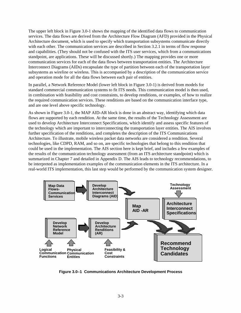
3-3
The upper left block in Figure 3.0-1 shows the mapping of the identified data flows to communicationservices. The data flows are derived from the Architecture Flow Diagram (AFD) provided in the PhysicalArchitecture document, which is used to specify which transportation subsystems communicate directlywith each other. The communication services are described in Section 3.2.1 in terms of flow responseand capabilities. (They should not be confused with the ITS user services, which from a communicationsstandpoint, are applications. These will be discussed shortly.) The mapping provides one or morecommunication services for each of the data flows between transportation entities. The ArchitectureInterconnect Diagrams (AIDs) encapsulate the type of partition between each of the transportation layersubsystems as wireline or wireless. This is accompanied by a description of the communication serviceand operation mode for all the data flows between each pair of entities.
In parallel, a Network Reference Model (lower left block in Figure 3.0-1) is derived from models forstandard commercial communication systems to fit ITS needs. This communication model is then used,in combination with feasibility and cost constraints, to develop renditions, or examples, of how to realizethe required communication services. These renditions are based on the communication interface type,and are one level above specific technology.
As shown in Figure 3.0-1, the MAP AID-AR block is done in an abstract way, identifying which dataflows are supported by each rendition. At the same time, the results of the Technology Assessment areused to develop Architecture Interconnect Specifications, which identify and assess specific features ofthe technology which are important to interconnecting the transportation layer entities. The AIS involvesfurther specification of the renditions, and completes the description of the ITS CommunicationsArchitecture. To illustrate, mobile wireless packet data networks are considered a rendition. Severaltechnologies, like CDPD, RAM, and so on, are specific technologies that belong to this rendition thatcould be used in the implementation. The AIS section here is kept brief, and includes a few examples ofthe results of the communication technology assessment (from an ITS architecture standpoint) which issummarized in Chapter 7 and detailed in Appendix D. The AIS leads to technology recommendations, tobe interpreted as implementation examples of the communication elements in the ITS architecture. In areal-world ITS implementation, this last step would be performed by the communication system designer.
Map DataFlows-CommunicationServices
DevelopArchitectureInterconnectDiagrams (AID)
DevelopNetworkReferenceModel
DevelopArchitectureRenditions(AR)
MapAID -AR
RecommendTechnologyCandidates
LogicalCommunicationFunctions
PhysicalCommunicationEntities
Feasibility &CostConstraints
ArchitectureInterconnectSpecifications
TechnologyAssessment
Figure 3.0–1 Communications Architecture Development Process

3-4
3.1 Communication Architecture
The generic communication hierarchical model presented in Figure 3.1-1 shows the relationship betweenthe Transportation and Communication Layers. Each data user can be one entity in the TransportationLayer (e.g., the Information Service Provider Subsystem or Personal Vehicle Subsystem in aninformation exchange). The user does not care about and should not be concerned with the specifics ofthis information transfer layer. In fact, the Communication Layer can be viewed as plumbing that carriesinformation from one user to another.
The complex makeup of the network is usually defined by system architectures developed to meetspecific requirements, performance objectives, and socio-economic drivers. In the absence of crispspecifications and because of the jurisdictional-independence of this particular architecture, the endframework precludes the design of low level implementation details. However, to properly evaluate thecommunication architecture candidates, select technologies and detailed designs are recommended in anevaluatory design (see the later chapters of this document.)
The generic hierarchical communication model shown in Figure 3.1-1 follows the Open SystemsInterconnection model which organizes the communication network in a highly structured format toreduce its overall design complexity. This model is structured as a series of layers each with the functionof providing certain services to the layer above and capable of conversing with the corresponding layer atthe other end of the link. Thus the high level layers (e.g., ITS application) are shielded from the actualimplementation details of the communication services. Different networks can use layers different fromthe OSI model, such as the IBM SNA (Systems Network Architecture). When different protocols areused in different networks, an interworking function must provide the conversion between the protocolsat the various levels.
The lowest layer in the OSI model is the physical layer (layer 1), which provides the transmission of bitsover wires or radio links.
Layer 2 is the data link layer, which is concerned with making the link appear to the receiver as bit error-free as possible by implementing error detection and correction (EDAC) coding schemes in thetransceiver. One example of this is the use of a cyclic redundancy code (CRC) to a block or frame of thedata. When the data passes the CRC check at the receiver, the returned acknowledgment indicateswhether re-transmission is needed.
Layer 3 is the network layer, which controls the operation of the network. Here, the key issue is routingpackets, which are also used to generate billing information for the communications service provider(billing is tied to IP addresses).
Layer 4 is the transport layer, which mediates between the session layer and the network layer, providingend-to-end accounting (sequencing, non-duplication, etc.) for all the data at the receiving end. It alsoisolates the top layers from the changing physical technologies.
Layer 5 is the session layer, which allows users on different machines to establish communications, orsessions, between them. This involves ordinary data transport but with enhanced services such as remotelog-in or file transfer.
Layer 6, the presentation layer, performs syntax and semantic operations on the information transmittedbetween the users, such as encoding data in a standard way, or compressing or encrypting that data.
Layer 7 is the application layer, which provides commonly used protocols for such tasks as terminalemulation, file transfer, electronic mail and remote job entry. (Note that for many ITS applications, layers5 and 6 are absorbed into the application layer, layer 7.)

3-5
123
4567
456
4567
456
Upper LayerProtocols
Upper LayerProtocols
Low LayerProtocols &Medium
ITSUSERA
NETWORK
Info InfoPotentialITSStandards
PotentialITSStandards
7 7
Transparent to Users
ITSUSERB
Figure 3.1-1 Generic Hierarchical Communication Model
From the Communication layer perspective, the term "services" is defined according to communicationsgoverning bodies (e.g., ITU, TIA, etc.), and should be used with care. That is, when describing acommunications architecture, one should not refer to Route Guidance or Pre-trip Planning as services.Rather, they are applications in need of a communication service. Elaborating more along these lines, ITSappears to the Communication Layer as a collection of applications with markedly differentcommunication requirements. Thus the service provided by the communication model is characterizedmore by 1) the application's directionality requirements (e.g., one-way or two-way) for informationtransport, 2) whether it is between mobile elements, mobile and stationary elements or stationaryelements, 3) the amounts of data to be transported, and 4) the urgency rather than the precise descriptionas Route Guidance or Pre-trip Planning.
The next section identifies various communication services to which the Transportation Layer data flowscan be matched. Subsequently, a matching process will assign broad generic communication services tothe ITS data flows without specifying a particular technology.
3.1.1 Communication Services
The communication services define the exchange of information between two points and are independentof the media and application (i.e., ITS user service). In essence, they are a specified set of user-information transfer capabilities provided by the communication layer to a user in the transportationlayer. Figure 3.1-2 illustrates the hierarchy of communication services. A brief description of the servicesis presented below; more detailed information is given in Appendix A.1.

3-6
Service
Conversational Messaging Broadcast Multicast
Interactive Distribution
Figure 3.1-2 Communication Services Hierarchy
Communication services consist of two broad categories, interactive and distribution. Interactive servicesallow the user to exchange data with other users or providers in real or near real time, asking for serviceor information and receiving it in the time it takes to communicate or look up the information.Distribution services allow the user to send the same message to multiple other users.
Interactive services may be either conversational or messaging. Conversational implies the use of a two-way connection established before information exchange begins and terminated when the exchange iscompleted. Messaging, on the other hand, works more like electronic mail being exchanged betweenusers. The messages are exchanged without establishing a dedicated path between the two sites. Eachmessage is addressed and placed on the network for transmission, intermixed with messages from otherusers. The communications community labels this mode of communication a “datagram” service.
Distribution services may be either broadcast or multicast and may be used over wireline and/or wirelesscommunication links. Broadcast messages are those sent to all users while multicast messages are sentonly to a subset of users. Multicast differs from broadcast in its use of a designated address for all usersand user groups. Examples of broadcast information might include current weather or road conditions,whereas multicast information might be information sent to all drivers working for a specific company. Achanging group membership could be the set of users traveling between two locations or with a certaindestination, for which unique information must be transmitted. The services that can be supported usingcircuit or packet connection mode include voice, video, image and data. (see Appendix A.1 for acomplete description.)
Not shown in the Figure 3.1-2 are location services. These fall in two categories: (1) the services that donot use the communication network (i.e., GPS, and stand alone terrestrial systems); (2) location servicesthat use the network for providing the service (e.g., cellular based systems). In the latter case, the locationservices fall under the interactive services. The service will be rendered by a service provider in responseto a request for information or help. (See detailed description in Appendix A.1).
3.1.2 Logical Communication Functions
Based on the objectives of the communication architecture, a list of logical functions to support the ITSsystem communication requirements are identified. The primary logical communication functions can beconfined to: wireless and wireline access, switching, routing, registration authentication, interworking,validation, billing, and operations (see Appendix A.2 for a detailed description).

3-7
3.1.3 Functional Entities
The functional entities that make up the communication layer were derived from existing and emerginginfrastructure specifications and standards (e.g., TIA, ITU, Bellcore, ANSI). These basic building blocksform the foundation of a generic communication system. As with the transportation layer, each functionalentity consists of one or more logical functions. These entities include: 1) user device, 2) user profilemodule, 3) switch, 4) wireless controller, 5) wireless base station, 6) interworking platform, 7) profiledata base, and 8) wireline network. A detailed description of these functional entities is presented inAppendix A.3.
3.1.4 Communication Network Reference Model
As shown previously in Figure 3.0-1, the communication architecture design process consists of severalsteps. The previous sections listed the communication logical functions and physical entities. Thearchitecture design process now starts on the lower leg of Figure 3.0-1 with the development of theCommunication Network Reference Model. This model provides an architecture or structure that showshow various communication technologies can implement the Architecture Interconnect Diagramsdeveloped in the next section.
The network reference model for ITS is depicted in Figure 3.1-3, and is a generic abstraction whichbuilds upon several reference models developed for standard commercial systems. Boxes represent thevarious physical equipment (with descriptive uppercase letters) that perform the communicationfunctions. The interfaces that are important to ITS are identified by lowercase letters (s, v, u1, u2, u3).
• s signifies a plug-in, smart card interface.
• v signifies any kind of wireline connection (for instance, RS-232) or even a bus if the UT and WT areintegrated.
The most important reference point is the wireless interface (u) connecting the WBS and the wirelesstransceiver. To meet the objectives of the national ITS Architecture it will be necessary in some cases forthe air interface to be standard. The wireless portion (u) of the architecture is manifested in threedifferent ways: u1, u2, u3. Each interface corresponds to one of the wireless manifestations as follows:
• u1 defines the wide area wireless airlink with one of a set of base stations providing connections tomobile or untethered users. It is typified by the current cellular telephone and data networks or thelarger cells of Specialized Mobile Radio for two way communication, as well as paging andbroadcast systems for one way communication.
• u2 defines the short-range airlink used for close-proximity (typically less than 50–100 feet)transmissions between a mobile user and a base station, typified by transfers of vehicle identificationnumbers at toll booths.
• u3 addresses the vehicle-vehicle (AHS-type) airlink, for high data rate, burst, usually line-of-sighttransmission with high reliability between vehicles where standards are in their infancy. Note that thewide area wireless (U1) interface encompasses both two-way (U1t) and broadcast (U1b) as shown inFigure 3.1-4.
• b, c, d, and e correspond to well-established wireline interfaces as documented in Section 7.5.2.

3-8
UPM UT WT
WT
WBS
WC
CS
PS
CS OAM&PPS
IWF
ISDN
PSTN
PDN
UT
Type 1
Type 2
Internet
Adapter
UT
UT
Signaling
UPM: User Profile Module UT: User Terminal DT: Dedicated Terminal WT: Wireless Transceiver WBS: Wireless Base Station WC: Wireless Controller CS: Circuit Switch PS: Packet Switch IWF: Interworking Function OAM&P: Operation, Administration, Management, Provisioning
s v u
uu
1
3 2
c
d
b e
DT
Figure 3.1.-3 Network Reference Model for the Communications Layer
The National ITS architecture provides for implementation flexibility. Various of the data flows in theArchitecture can be carried over a multiple of these interfaces, and the final choices would be made bythe local implementors. This flexibility is depicted conceptually in Figure 3.1.-4.
U1: Wide-area Wireless
U1b:Broadcast
U3: Short range (V-V) wireless
U1t: Two-way
U2: Short Range (DSRC) wireless
Figure 3.1-4 Implementation Flexibility of ITS Architecture Data Flows

3-9
Since the wireline segment encompasses standard wireline configurations, the ITS-critical elements froma standards perspective are those comprising the wireless portion on the left side of Figure 3.1-3. Thewireless portion consists of the User Profile Module (UPM), the User Terminal (UT), the WirelessTransceiver (WT) and the Wireless Base Station (WBS). The connections through the DedicatedTerminal and various User Terminals are shown in the column of boxes on the right. The equipment inthe center is the existing public telecommunications services, so the details are transparent to ITS, whichis a major benefit to the ITS community. All management, operations, expansion, and improvement costsare shared with the wider set of all telecommunications users.
This is an important point to jurisdictions and agencies who prefer to procure and trench their ownnetwork along the right-of-way. Whereas a financial sensitivity analysis may point to a private solution, itfrequently does not fully consider the large and sustained Operation, Administration, Management , andProvisioning (OAM&P) fees that the agency will have to pay the telecommunications vendor during thesystem's life cycle.
Appendix A.4 presents a detailed description of the wireline side of the above network reference model,in addition to a more thorough treatment for required interfaces such as switches, controllers, andterminals. Appendix A.4 also presents the network entities, interfaces, and signaling plane, and includesa discussion on circuit connection and data packet transmission.
3.2 Communication Layer Linkage
This Communication Layer Linkage section further identifies the relationship between the TransportationLayer and Communication Layer definitions. This is accomplished by mapping the communicationservices to the data flows identified in the Transportation Layer, generating the Architecture InterconnectDiagrams (AIDs), identifying the Architecture Renditions (ARs), mapping the AIDs to the ARs, andfinally identifying the Architecture Interconnect Specifications (AISs) based on the technologyassessment.
3.2.1 Mapping Communication Services to Data Flows
Mapping of the communication services to the data flows establishes the first link between thetransportation layer and the communication layer. This initial link depends on the completion of twotechnical architecture milestones. First, the message sizes and data transfer requirements are broadlyidentified. Second, the physical architecture that allocates logical functions (see Logical ArchitectureDocument) to subsystems necessitates a partitioning exercise which defines the data flows that requirecommunication. This mapping is an iterative procedure that is calibrated by feedback from the logicaland physical architectures (and in turn the ITS stakeholders) by retracing the steps shown in Figure 3.0-1.
Appendix A.5 details the mapping process. It also depicts the assigned communication service for eachdata flow with the corresponding rationale.
3.2.2 Architecture Interconnect Diagrams
As denoted in Figure 3.1-1, this section presents the development of the Architecture InterconnectDiagrams (AIDs). These diagrams show the subsystem-to-subsystem communication interfaces of alltransportation subsystem entities (defined in the transportation part of the Physical Architecture). Thediagrams identify the communication mode and partition, either wireline or one of three types of wirelessconnection, as well as documenting the rationale for each of these choices when needed for clarification.The diagrams identify the requirements, developed from the physical relationships of the various

3-10
subsystem entities, but do not advocate any specific communication technology to be used. Theinformation contained in the AIDs can be traced to the information provided in the Data Flow-Communications Service Mapping Table (Appendix A.5).
A template is used to illustrate the interconnections between entities and between modules (described inthe next sub-section). At this stage in the physical architecture, no AIDs are defined for inter-moduleinformation transfer within a simple entity. In fact, from the communication layer perspective, this is notnecessary. The most important goal is to identify the inter-entity interconnectivity.
The subsections that follow describe the AID template, and present the Level 1 and Level 0 (top level)AID’s.
3.2.2.1 AID TemplateAs depicted in Figure 3.2-1, each AID shows the two communicating transportation subsystem entities,the interconnection partition (i.e., wireline, wireless, or both), and a characterization of theinterconnection. The latter is not a link-specific description, which the AIS provides, but a high-levelinterpretation in terms of services and operation modes. When not obvious, the choice of operation modeis based on the rationale provided in Table 3.2-1. The interconnect description for each AID provides adata flow and a service and operation mode description for each data flow between the two entities. TheData Flow information also provides directionality when more than one data flow exists between theentities, not all of which are in the same direction. If all the data flows are in the same direction, noindication is given and the data flows from the left entity to the one on the right.

3-11
Entity Interconnect Partition Entity
∧Interconnect Description
Data Flow:
Service
Operational Mode
Figure 3.2-1. Template for the Architecture Interconnect Diagram (AID)
3.2.2.2 Level 1 AIDsUsing the AID template and Table A.5-1, Data Flow – Communication Services Mapping Table(located in Appendix A of this document), the data flows are represented in an ArchitectureInterconnect Diagram (AID) format. A single example is presented here in Figure 3.2-2, andvarious others are compiled in Appendix B.
EmergencyManagementSubsystem(EM)
Wireless wide area interface (U1)EmergencyVehicleSubsystem(EVS)
Bursty data or live speech.∧DataFlow:
Emergency dispatch requestsEmergency vehicle dataRoute request
----><----<----
Service Conversational speech,Messaging data
Operational Mode
Circuit, Packet
Figure 3.2-2 Example of AID Level-1

3-12
3.2.2.3 Level 0 AIDFigure 3.2-3, shows the Level 0 Architecture Interconnect Diagram (AID). The level 0 AID is apercolation to a top level of all the detailed, level 1 AID’s. It presents the all the interfaces between thephysical subsystem entities, capturing the wireline (w) or wireless (u1, u2, or u3) nature of the interfaces inthe ITS architecture. As such, it is a comprehensive, albeit not complete, representation of the ITScommunication architecture. More detailed variations can be easily derived from it. For example, Figure3.2-4 shows the data flows using the u1b wide area wireless broadcast “sub-interface”. Figure 3.2-5shows the subset that uses either of u1t (two-way wide area wireless) or u1b (wide area wirelessbroadcast). Note that u1b does not imply a certain technology. FM subcarrier, paging, and messagingdata networks are possible implementations and they all tend to use a broadcast protocol in the forward,i.e.; fixed to mobile, direction.

3-13
Wide Area Wireles Interface (u1t and u1b)Short Range Vehicle to Roadside Wireless Interface (u2) Vehicle to Vehicle Wireless Interface (U3)
Legend
PS
Wire line (W)u1t, u1b & WPlanning Subsystem (W)
PS
PS
PS
Other VS
CENTERInformationService ProviderSubsystem (ISP)
PS
CENTERToll AdministrationSubsystem TAS
CENTEREmission ManagementSubsystem (EMMS)
CENTERFleetMangementSubsystem(FMS)
ROADSIDECommercialVehicle CheckSubsystem (CVCS)
VEHICLEVehicleSubsystem (VS)
CENTEREmergencyManagementSubsystem (EM)
CENTERTransit ManagementSubsystem (TRMS)
PS
PS
PS
Remote AccessPersonal Inf.Access Subsystem(PIAS)
Remote AccessRemote TravelerSupport Subsystem(RTS)
ROAD SIDERoadway
Subsystem (RS)
ROADSIDEToll CollectionSubsystem (TCS)
ROADSIDEParking ManagementSubsystem (PMS)
CENTERTraffic ManagementSubsystem (TMS)
VEHICLEEmergency Vehicle Subsystem (EVS)
Other TRVS
VEHICLETransit VehicleSubsystem (TRVS)
VEHICLECommercialVehicle Subsystem(CVS)
Other CVS
Other EVS
PS
CENTERCommercialVehicle Adm.Subsystem(CVAS)
Figure 3.2-3 Level 0 Architecture Interconnect Diagram for the National ITS Architecture

3-14
CENTERTransit ManagementSubsystem (TRMS)
Remote AccessPersonal Inf.Access Subsystem(PIAS)
Remote AccessRemote TravelerSupport Subsystem(RTS)
TRAFFIC DATA FOR PORTABLESTRANSIT DEVIATION FOR PORTABLES
TRAFFIC DATA FOR KIOSKSTRANSIT DEVIATION FOR KIOSKSTRAVELER TRIP INFORMATIONTRAVELER YELLOW PAGES DATA ADVISORY DATA
BROADCAST DATALINK AND QUEUE DATAYELLOW PAGES ADVISORY DATA
TRANSIT SERVICES FOR PORTABLES
CENTERInformationService ProviderSubsystem (ISP)
VEHICLEVehicleSubsystem (VS)
Figure 3.2-4 Level 0 Architecture Interconnect Diagram for the National ITS Architecture
(Subset showing U1b data flows)

3-15
CENTERInformationService ProviderSubsystem (ISP)
CENTERTransit ManagementSubsystem (TRMS)
Remote AccessPersonal Inf.Access Subsystem(PIAS)
TRANSIT DEVIATION FOR PORTABLES
TRAVELER TRIP INFORMATIONTRAVELER YELLOW PAGES
ADVISORY DATAYELLOW PAGES ADVISORY DATA
TRANSIT SERVICES FOR PORTABLES
Remote AccessRemote TravelerSupport Subsystem(RTS)
VEHICLEVehicleSubsystem (VS)
Figure 3.2-5 Level 0 Architecture Interconnect Diagram for the National ITS Architecture;
(Subset showing data flows using either U1t or U1b)

3-16
3.2.3 Architecture Renditions
The next step in the communications architecture design process is the development of thecommunication Architecture Renditions, as depicted in Figure 3.0-1. Combining elements from theGeneric Heirarchical Communication Model (Figure 3.1-1) and the ITS Communication NetworkReference Model (Figure 3.1-3) provides a more detailed view of the flow of information between twousers. This information includes communication services and operational modes (i.e., circuit switched,packet switched, etc.). The architecture renditions are essentially examples of how to provideconnections between users based on the communications network reference model and the evaluations ofclasses of feasible implementations.
Two levels of renditions are generated. A Level 1 rendition is generated for each of the possibleinterconnections between services. The Level 0 Rendition (the top level) shows the full connectivitybetween users over multiple links. The details of the renditions, how they are generated, and those thatapply to the different interconnections in the architecture are provided in Appendix C. An example of aLevel-1 rendition and the Level-0 will be provided here to support the subsequent task of AIS generation.
3.2.3.1 Level 1 RenditionFigure 3.2-6 depicts Level 1 renditions for the two-way wide-area wireless communication link (u1)through switched networks. This figure depicts interconnection between tetherless users or tetherless andstationary users, utilizing two distinct classes of two-way wide-area wireless technologies. Severaltechnologies or systems can fit within each rendition. For example, CDPD, RAM, ARDIS and so on arepossibilities for implementing the packet-switched wireless data network rendition (shown on the right-hand-side of the diagram in Figure 3.2-6).
WIRELESS CONTROLLER
OTHER PACKET SWITCH
BASE STATIONs• • •
FIXED NETWORK
OAM&P
1
USER TERMINAL • • •
MODEM BANK
PACKET SWITCH
CIRCUIT SWITCH
OTHER CIRCUIT SWITCH
USER TERMINAL
USER TERMINAL
T1
Packet mode Rendition for U1 supports: - messaging data, - multicast data, - broadcast data
Circuit mode Rendition for U1 supports: - conversational speech, - conversational data
u
Figure 3.2-6 Rendition 1 — Wide-Area Wireless (u1) Link Through Switched Networks

3-17
Figure 3.2-7 depicts the rendition for wide area one way wireless link u1b. It uses broadcast systemswhich include paging and FM subcarrier technologies for transmitting data to subscribers over the pagingand FM frequency channels, respectively.
Broadcast Message Processor
FM Broadcast StationsData Encoder &
Subcarrier Generator
Data Distribution Network
Message EntrySystem
UserTerminal
UserTerminal
UserTerminal
U1b
Broadcast Mode Renditionfor U1b support: - Broadcast Data
Paging Broadcast StationsData Encoder & Modulator
Figure 3.2-7 Rendition 1 for Wide-Area One-Way Wireless (u1b) Links
3.2.3.2 Level 0 RenditionFigure 3.2-8 illustrates the Level 0 rendition. It represents a composition of all the renditions to reflectthe combined needs of the architecture. This rendition shows a user communicating to another user,central office or a base station over various communication links such as u1, u2, u3 and w. Again, thedetails of this mapping are provided in Appendix C.1.1.

3-18
User
Central Office
Base Station
Base Station
Rendition 1
u1
w, u1
Rendition 2
u2
w
Rendition 4
w
Rendition 3
u3
Candidate Technologiesfor u1 interface
(Example)Terrestrial systems•FM subcarrierCellular based systems•CDPD•ESMR, RAM, ARDIS•Two-way paging
Candidate Technologiesfor w interface
(Example)Public Networks•PSTN, ISDNPrivate networks•SONET, ATM
Candidate Technologiesfor u2 interface
(Example)•Active RF•Passive RF•Infrared
User
User
Figure 3.2-8 Level 0 Rendition
3.2.4 Architecture Interconnect Specifications
The Architecture Interconnect Specifications (AISs) are now developed from the technology assessmentand refined by combining the renditions with applicable technologies and evaluating the achievableperformance (Figure 3.0-1). This involves mapping the applicable communication technologies to therenditions.
To facilitate the mapping of the communication technologies to the renditions, the candidate wireless andwireline technologies are surveyed. The candidate technologies are further assessed and theirperformance is evaluated from the National ITS Architecture standpoint. For example, the assessmentincludes: short range and wide area, one-way and two-way wireless data communication. Systemsanalyzed include terrestrial networks (e.g., cellular, ESMR), FM broadcast, and satellite systems formobile and fixed services. The details of this survey, as well as the sources of information, are presentedin Appendix D; the assessment results are summarized in Chapter 7.

3-19
The results of this assessment are used in identifying the candidate technologies to support level 0 andlevel 1 renditions. The results of this mapping are summarized below.
It is apparent from the matrices provided in the Technology Assessment Section (Section 7.5) that for theforeseeable future, wireless data networks (such as CDPD, RAM, etc.) form the class of communicationsystems most suitable to interactive wide area wireless ITS links (u1t). The infrastructure is alreadylargely available (short, in some areas, of adding the appliqué equipment). Service costs are already low,and equipment costs are coming down. Coverage nationally is excellent with the possible shortcomingthat it may not be available for some time in rural and remote areas. Yet, with the advent of innovativesolutions like circuit-switched CDPD – which utilizes the AMPS cellular infrastructure in a mannertransparent to a CDPD subscriber – this problem would be largely mitigated. In any event, for ITS userswho insist on uninterrupted coverage in remote areas, holes in the coverage of terrestrial cell-basedsystems can be supplemented by satellite communication systems.
Figure 3.2-9 depicts the use of CDPD in a u1 communication architecture rendition to create an exampleof Architecture Interconnect Specification.
According to internal market research and analysis, users are concerned with two overshadowing factors:cost and quality. The Architecture Development Team believes that the market will determine thewinning technologies which will gain wide scale acceptance.
WIRELESSCONTROLLER
BASESTATIONs
USERTERMINAL
PACKETSWITCH
CIRCUITSWITCH
CDPD/Analog Cellular over U1 supports: - Conversational Speech - Conversational Data - Messaging Data - Multicast Data
CDPD/AnalogCellular
CDPD/AnalogCellular
TCPIP
MDLPIS-3
CLNP
(same physical layeras analog cellular)
1tu
Figure 3.2-9 AIS Example Using CDPD for Wide Area Wireless (u1)
Table 3.2-1 provides an illustration of candidate technologies for the different wireless data flows withinthe context of the communication layer of the ITS Architecture. In addition to wireless data networks, forwide area ITS data flows, the short range wireless interface u2 comprises a distinct set of communicationservices and supporting radio technologies. In a real world ITS implementation, the system designermakes use of the technology assessments of Chapter 7, and the ITS architecture communicationrenditions presented above, to select the specific communication systems/technologies most appropriatefor the deployment at hand.

3-20
Table 3.2-1 Examples of Candidate Technologies for Wireless Data Flows
u1t - Packet switched wireless data (e.g., CDPD, RAM, ARDIS) forwide-area wireless interface
(messaging services; bursty data transfers)Source Architecture Flow DestinationCVAS Electronic credentials FMSCVAS Safety information CVCSCVS Driver & vehicle information FMSCVS On board vehicle data FMSEM emergency dispatch requests EVSEM emergency acknowledge VSEM emergency acknowledge RTSEM emergency acknowledge PIASEVS Emergency vehicle driver
status updateEM
EVS Emergency vehicle driver input EMEVS Emergency vehicle dispatch
acknowledgeEM
FMS fleet to driver update CVSPIAS Demand responsive transit
requestTRMS
PIAS Traveler information request ISPPIAS Emergency notification EMRTS Emergency notification EM
TRMS Demand responsive transitrequest
PIAS
TRMS Request for vehicle measures TRVSTRMS Route assignment TRVSTRVS Emergency notification TRMSTRVS Vehicle probe data TRMSTRVS Traveler information request TRMS
VS vehicle probe data ISPVS emergency notification EMVS Traveler information request ISPVS map update request X23
u1t - Circuit switched wireless data (e.g., Cellular, ESMR)(Messaging; larger data transactions, e.g., compressed image)
Source Architecture Flow DestinationISP Traveler information PIASISP Traveler information VSX23
MAP UpdateProvider
Map updates PIAS
X23MAP Update
Provider
Map updates VS

3-21
u1t - Circuit Switched Voice (e.g., Cellular, SMR)(live voice interaction; early implementations)
Source Architecture Flow DestinationEM Assigned route EVSEM Hazmat information EVSEM Emergency dispatch
requestsEVS
EM Emergency status RTSEVS Emergency vehicle dispatch
acknowledgeEM
EVS Emergency vehicle driverinput
EM
RTS Emergency notification EMVS Emergency notification EM
u1b - Broadcast (subcarrier or paging-type) services (Broadcast of free services and services that require subscription;
e.g., traveler information,)source Architecture Flow destination
ISP Broadcast information PIASISP traveler information VSISP broadcast information VSISP broadcast information RTS
u1t - Packet switched wireless data multicast Services (Distributionservices that require subscription; e.g., map updates)
source Architecture Flow destinationISP traveler information PIASISP traveler information VSISP broadcast information VSISP broadcast information RTSX23
MAP updateprovider
map updates PIAS
X23MAP update
provider
map updates VS
u2 - beacon for close-proximity wireless communication betweenvehicle and roadside
Source Architecture Flow DestinationCVS Border crossing ID CVCSCVS on board safety data CVCS
CVCS safety inspection record CVSCVCS Pull in message CVSEVS Emergency vehicle
preemption requestRS
PMS Tag update VSRS AHS control data VSRS roadway signage data VSRS intersection status VS
TCS Request tag data VSTRVS signal priority request RS
VS Tag data TCSVS AHS vehicle data RSVS Tag data PMS

4-1
4. SCENARIOS AND TIME FRAMES
Three scenario regions will be studied (Urbansville, Thruville, and Mountainville), for three timeframes (1997, 2002, and 2012). These nine total scenarios were modeled through the use ofgovernment-supplied information, along with statistical data and assumptions related to theevaluatory design that is a subset of the National ITS Architecture definition effort.
The goal of this part of the modeling task is to determine the number of users of each of the userservice groupings defined for the data loading analysis task. In most cases, this is the number ofvehicles because most of the messages are handled per vehicle. The exception is the travelerinformation user (PIAS user) service group where no user vehicle is involved.
Because communications systems must be designed for the peak load, the important number ofusers to be derived is that for the peak period. The off-peak period number will be defined as afraction of the peak period number.
4.1 Evaluatory Design
The evaluatory design is a candidate ITS deployment with a set of assumptions for the number ofusers and vehicles, and the number of centers, sensors, etc. The important assumptions in thewireless data loading are the number of vehicles and users for each of the user service groups.The total set of assumptions for the evaluatory design are contained in the Evaluatory DesignDocument.
4.2 Baseline Information for the Scenario Regions
The information supplied by the Government on the nine scenario regions and time framesincludes the regional population and number of household vehicles. This information was usedalong with national statistical data to derive the number of vehicles or users that are potentialusers of ITS services by user service category within each scenario. Table 4.2-1 lists the suppliedpopulation and vehicle data.
Table 4.2-1 Supplied Population and Household Vehicle Data
Region Time Frame Population Household Vehicles
Urbansville 1997 2814950 1688970
Urbansville 2002 3106674 1842105
Urbansville 2012 3788627 2273176
Thruville 1997 1005185 851272
Thruville 2002 1055445 893836
Thruville 2012 1166015 987476
Mountainville 1997 17480 6735
Mountainville 2002 17920 6904
Mountainville 2012 18845 7260

4-2
4.3 Number of Potential Users by User Service Group
In order to enhance the understanding of the data loads generated by ITS services, the analyseswere performed for seven distinct user service groups, each with its own population, message set,peak period definition, and message frequency of use. The user service groups include privatevehicles, CVO-Local vehicles, CVO-long haul vehicles, travelers (PIAS users), transitmanagement, emergency management, and probes.
The number of potential users that might buy a service was determined for each of the ninescenarios through the use of national statistics. The methods used are shown in detail inAppendix E. The numbers are the same as those found in the Evaluatory Design Document.
The lack of a particular service (e.g., fixed route transit in the rural scenario) was handledlater in the data loading models with the lack of an entry in the database table of marketpackages of services for that scenario, preventing messages related to that service frombeing included in the message set for that scenario. This process is defined in Section 5.3, asit defines the available message set for that scenario.
In the case of the Thruville scenario, the added traffic traveling completely through the entirescenario region must be added to the model. This was modeled by increasing the number ofprivate vehicles and CVO long haul vehicles that would be expected from the resident population(as derived from national statistics) by one-third. The other user service groups do not travelbeyond the scenario region by definition.
The number of potential users was derived for the peak period defined for that particular userservice group. The number of potential users for the off-peak period was then defined as afraction of the peak period number.

4-3
Number of Potential Users Summary
Table 4.3-1 shows the summary of the number of potential users for each of the nine scenarios.These are the same values as in the Evaluatory Design Document.
Table 4.3-1 Number of Potential Vehicles or Users for Each of the Seven User ServiceGroups and Each of the Nine Scenarios.
Pr. Veh. CVO-LH CVO-Lo. Trav. Transit Emerg. Probes
Urbans.
1997
760037 5797 81155 200750 1661 4444 7704
Urbans.
2002
828947 6397 89565 262920 1833 4850 7704
Urbans.
2012
1022929 7802 109226 432310 2235 5981 7704
Thru.
1997
383072 2753 28979 99610 593 2128 3900
Thru.
2002
402226 2891 30428 125500 623 2319 3900
Thru.
2012
444364 3194 33616 184870 688 2562 3900
Mount.
1997
3031 36 504 830 0 7 800
Mount.
2002
3107 37 517 1010 11 7 800
Mount.
2012
3267 39 543 1420 11 8 800
4.4 Penetrations
A penetration factor was applied to each of the potential number of users figures to arrive at theactual number of users. The penetrations were applied by market package for the 1997, 2002, and2012 time frames. These penetrations are from the Evaluatory Design Document, using the“high” penetration estimate for the equipment package most appropriate for that market package.The penetration factors for market packages by time frame are shown in Table 4.4-1. Each of theseven user service groups was allowed access to any of the market packages that were of use tothem. The penetration is applied to the frequency of use value that is assigned later to eachmessage for each user service group to account for the variations in the amount of usage thatmight occur in the user service groups. The result is that the messages each have a penetrationvalue associated with them. There is not simply a single penetration value for an entire userservice group.

4-4
Table 4.4-1 Penetration Factor by Market Package and Time Frame
Market Packa ge Name 1997 2002 2012Transit Vehicle Tracking 0.33 1 1Transit Fixed-Route Operations 0.66 1 1Demand Response Transit Operations 0.66 1 1Transit Passenger and Fare Management 0.66 1 1Transit Security 0.33 1 1Transit Maintenance 0.66 1 1Multi-modal Coordination 0.66 1 1Broadcast Traveler Information 0.03 0.1 0.5Interactive Traveler Information 0.01 0.1 0.2Autonomous Route Guidance 0.01 0.1 0.2Dynamic Route Guidance 0.01 0.1 0.2ISP Based Route Guidance 0.01 0.1 0.2Integrated Transportation Management/Route Guidance 0.01 0.1 0.2Yellow Pages and Reservation 0.01 0.1 0.2Dynamic Ridesharing 0.01 0.1 0.2In Vehicle Signing 0 0.01 0.05Network Surveillance 0.004 0.02 0.05Probe Surveillance 0.004 0.02 0.05Surface Street Control 0.2 0.5 0.9Freeway Control 0.75 1 1HOV and Reversible Lane Management 0.07 0.2 0.4Traffic Information Dissemination 1 1 1Regional Traffic Control 0 0 1Incident Management System 1 1 1Traffic Network Performance Evaluation 0.5 1 1Dynamic Toll/Parking Fee Management 0.5 0.75 1Emissions and Environmental Hazards Sensing 1 1 1Virtual TMC and Smart Probe Data 0.004 0.02 0.05Vehicle Safety Monitoring 0.02 0.2 0.5Driver Safety Monitoring 0 0.05 0.25Longitudinal Safety Warning 0 0.02 0.15Lateral Safety Warning 0 0.05 0.15Intersection Safety Warning 0 0.001 0.02Pre-Crash Restraint Deployment 0 0 0.05Driver Visibility Improvement 0 0 0.05Advanced Vehicle Longitudinal Control 0 0.02 0.15Advanced Vehicle Lateral Control 0 0 0.05Intersection Collision Avoidance 0 0 0.02Automated Highway System 0 0 0.01Fleet Administration 0.25 0.5 0.8Freight Administration 0.05 0.1 0.5Electronic Clearance 0.25 0.5 0.85CV Administrative Processes 0.25 0.5 0.85International Border Electronic Clearance 0.25 0.5 0.85Weigh-In-Motion 1 1 1Roadside CVO Safety 1 1 1On-board CVO Safety 0 0.02 0.1CVO Fleet Maintenance 0.05 0.1 0.5HAZMAT Managment 0.05 0.1 0.5Emergency Response 0.5 1 1Emergency Routing 0.5 1 1Mayday Support 0.5 1 1ITS Planning 0 1 1

4-5
4.5 Assignment of Users to Communications Interfaces
Messages are assigned to flow over any appropriate communications media, and individualmessages are allowed to flow over multiple media. The u1t interface is the wide area two-waywireless interface, and the u1b interface is the wide area broadcast interface. The u2 interface isthe short range vehicle-to-roadside wireless interface. The w interface is the wireline interface.
Messages shared between the u1t and u1b interfaces include traffic advisories and data, andtransit deviations and services. In order to study the worst case, it was assumed in the dataloading analysis that the broadcast transmission does not reduce the use of u1t data traffic.Therefore, the u1t fraction may be shown as 1 in cases where a message is assigned to otherinterfaces as well.
Messages shared between the u1t and u2 interfaces include transit management and services, andparking advance payment. In order to study the worst case, it was assumed in the data loadinganalysis that the u2 transmissions do not reduce the use of u1t data traffic.
For the case of messages shared between the u1t and w interfaces, it was assumed that 50% ofthe traveler user service group (PIAS users) use the w interface and 50% use the u1t interface. Itwas also assumed that 90% of the kiosks are connected over the w interface, and 10% use the u1tinterface. In addition, 90% of the commercial vehicle check subsystems and fleet managementsubsystems use a wireline interface, and 10% use the u1t interface, because they are not at fixedlocations. In the case of very large messages, it was decided not to include them on all applicableinterfaces. For example, messages (flows) for map updates, including the associated requests andpayment responses were not included on the u1t interface because their large size would make itunlikly that any user would choose that means of update. A wireline connection, such as duringan evening, or substitution of an updated CD are the assumed map update mechanisms. Anotherexample is “link_and_queue_data”, which, because of its size, is assigned to the u1b interface.
Map and link + queue data updates of a more limited geographic extent, or incremental updates,when included in future versions of the logical architecture would make sense for the u1tinterface.
The message “vehicle_guidance_probe_data” from VS to ISP appears in its own user servicegroup, probes. Finally, it was assumed that display and map updates, because of their very largesize (and therefore transmission cost) would not be used by any of the above users unlessconnected at that moment by wireline access. They would simply choose to perform updateswhile connected over a w interface or use another transfer media such as a CD.
The message assignments to interfaces are shown in Table 4.5-1. They are sorted by physicalarchitecture source and sink. An “x” is placed in the interfaces over which a particular message isallowed to flow in this analysis. The column labeled “u1t Fraction” indicates the fraction of thatmessage’s data that is assigned to the u1t interface. The balance is assigned to the otherinterface(s). In a few cases, the u1t Fraction value was reduced on some individual messagesrelative to others for that user type to include a factor to account for the lower usage of aparticular user service feature because, for instance, it is less suitable for use from a mobilelocation (e.g., ISP to VS message advisory_data, which is large and will be costly to transmit onthe u1t interface, is assigned a fraction of 0.5 instead of 1).

4-6
Table 4.5-1 Communications Interfaces Assigned to Each of the MessagesNote: Data flows to terminators are all wireline (w).
PASource
PA Sink Message Data Flow u1t u1tFraction
u1b u 2 u3 w
CVAS CVCS cv_credentials_database_update x 0.1 x
CVAS CVCS cv_credentials_information_response x 0.1 x
CVAS CVCS cv_safety_database_update x 0.1 x
CVAS CVCS cv_safety_information_response x 0.1 x
CVAS FMS cf_clearance_enrollment_confirm x 0.1 x
CVAS FMS cf_enrollment_information x 0.1 x
CVAS FMS cf_enrollment_payment_confirmation x 0.1 x
CVAS FMS cv_enrollment_information x 0.1 x
CVAS FMS cv_enrollment_payment_confirmation x 0.1 x
CVAS PS cv_operational_data x
CVCS CVAS cv_credentials_information_request x 0.1 x
CVCS CVAS cv_roadside_daily_log x 0.1 x
CVCS CVAS cv_safety_information_request x 0.1 x
CVCS CVAS cv_update_safety_problems_list x 0.1 x
CVCS CVS cv_inspection_data_output x
CVCS CVS cv_on_board_pull_in_output x
CVCS CVS cv_on_board_screening_record x
CVCS CVS cv_request_electronic_clearance_data x
CVCS CVS cv_request_on_board_data x
CVS CVCS cv_electronic_clearance_data x
CVS CVCS cv_on_board_data x
CVS FMS cf_driver_route_instructions_request x 1
CVS FMS cf_on_board_vehicle_data x 1
CVS FMS cv_driver_enrollment_payment_request x 1
CVS FMS cv_driver_enrollment_request x 1
CVS FMS cv_driver_route_request x 1
CVS FMS cv_driver_storage_request x 1
CVS FMS cv_static_route_data x 1
EM EVS emergency_vehicle_driver_outputs x 1
EM FMS cf_hazmat_request x 0.1 x
EM ISP emergency_vehicle_route_request x
EM ISP incident_information x
EM PIAS emergency_request_personal_traveler_acknowledge x 0.5 x
EM PS emergency_vehicle_operational_data x
EM RTS emergency_request_kiosk_traveler_acknowledge x
EM TMS emergency_vehicle_green_wave x
EM TMS incident_details x
EM TMS incident_response_status x
EM TRMS transit_incident_coordination_data x
EM VS emergency_request_driver_acknowledge x 1
EM VS emergency_request_vehicle_acknowledge x 1
EMMS PS pollution_operational_data x
EMMS RS pollution_state_vehicle_acceptance_criteria x
EMMS TMS pollution_incident x
EMMS TMS pollution_state_data x
EMMS TMS wide_area_pollution_data x
EVS EM emergency_driver_dispatch_acknowledge x 1
EVS EM emergency_driver_status_update x 1

4-7
Table 4.5-1 Communications Interfaces Assigned to Each of the MessagesNote: Data flows to terminators are all wireline (w).
PASource
PA Sink Message Data Flow u1t u1tFraction
u1b u 2 u3 w
EVS EM emergency_vehicle_driver_inputs x 1
EVS RS emergency_vehicle_preemptions x
FMS CVAS cf_enroll_clearance_data x 0.1 x
FMS CVAS cf_enrollment_payment_request x 0.1 x
FMS CVAS cf_enrollment_request x 0.1 x
FMS CVAS cv_enrollment_payment_request x 0.1 x
FMS CVAS cv_enrollment_request x 0.1 x
FMS CVS cf_driver_route_instructions x 1
FMS CVS cf_request_on_board_vehicle_data x 1
FMS CVS cv_driver_enrollment_information x 1
FMS CVS cv_driver_enrollment_payment_confirmation x 1
FMS CVS cv_driver_route_data x 1
FMS CVS cv_static_route_request x 1
FMS EM cf_hazmat_route_information x 0.1 x
FMS EM cf_hazmat_vehicle_information x 0.1 x
FMS ISP cf_route_request x 0.1 x
FMS ISP cv_route_request x 0.1 x
ISP EM emergency_vehicle_route x
ISP EM incident_information_request x
ISP FMS cf_route x 0.1 x
ISP FMS cv_route x 0.1 x
ISP PIAS traffic_data_for_portables x x
ISP PIAS transit_deviations_for_portables x 0.05 x x
ISP PIAS traveler_guidance_route x 0.05 x
ISP PIAS traveler_map_update_payment_response 0.5 x
ISP PIAS traveler_personal_display_update_payment_response x
ISP PIAS traveler_personal_payment_confirmation x 0.5 x
ISP PIAS traveler_personal_transaction_confirmation x 0.5 x
ISP PIAS traveler_personal_trip_information x 0.05 x
ISP PIAS traveler_personal_yellow_pages_data x 0.5 x
ISP PMS advanced_other_charges_request x
ISP PMS advanced_traveler_charges_request x
ISP PMS parking_lot_data_request x
ISP PMS parking_lot_reservation_request x
ISP PS current_other_routes_use x
ISP PS current_other_routes_use x
ISP PS current_road_network_use x
ISP RTS advanced_tolls_and_charges_roadside_confirm x 0.1 x
ISP RTS traffic_data_for_kiosks x x
ISP RTS transit_deviations_for_kiosks x x
ISP RTS traveler_payment_confirmation x 0.1 x
ISP RTS traveler_transaction_confirmation x 0.1 x
ISP RTS traveler_trip_information x 0.1 x x
ISP RTS traveler_yellow_pages_data x 0.1 x x
ISP TAS advanced_other_tolls_request x
ISP TAS advanced_traveler_tolls_request x
ISP TMS commercial_vehicle_incident x
ISP TMS confirm_incident_data_output x

4-8
Table 4.5-1 Communications Interfaces Assigned to Each of the MessagesNote: Data flows to terminators are all wireline (w).
PASource
PA Sink Message Data Flow u1t u1tFraction
u1b u 2 u3 w
ISP TMS current_other_routes_use x
ISP TMS current_road_network_use x
ISP TMS current_transit_routes_use x
ISP TMS low_traffic_route x
ISP TMS media_incident_data_updates x
ISP TMS request_incident_media_data x
ISP TMS traffic_data_media_request x
ISP TRMS advanced_other_fares_request x
ISP TRMS advanced_tolls_and_charges_vehicle_confirm x
ISP TRMS advanced_traveler_fares_request x
ISP TRMS paratransit_service_confirmation x
ISP TRMS paratransit_trip_request x
ISP TRMS request_prices x
ISP TRMS transit_services_advisories_request x
ISP TRMS transit_services_guidance_request x
ISP TRMS transit_vehicle_deviations_details_request x
ISP VS advanced_fares_and_charges_response x 1
ISP VS advanced_tolls_and_fares_response x 1
ISP VS advisory_data x 0.5 x
ISP VS broadcast_data x
ISP VS link_and_queue_data x
ISP VS yellow_pages_advisory_data x 1 x
PIAS EM emergency_request_personal_traveler_details x 0.5 x
PIAS ISP traffic_data_portables_request x 0.5 x
PIAS ISP transit_deviations_portables_request x 0.5 x
PIAS ISP traveler_map_update_payment_request x
PIAS ISP traveler_personal_current_condition_request x 0.5 x
PIAS ISP traveler_personal_display_update_payment_request x
PIAS ISP traveler_personal_payment_information x 0.5 x
PIAS ISP traveler_personal_transaction_request x 0.5 x
PIAS ISP traveler_personal_trip_confirmation x 0.5 x
PIAS ISP traveler_personal_trip_request x 0.5 x
PIAS ISP traveler_personal_yellow_pages_information_request x 0.5 x
PIAS ISP traveler_route_accepted x 0.5 x
PIAS ISP traveler_route_request x 0.05 x
PIAS TRMS transit_services_portables_request x 0.5 x
PMS ISP advanced_other_charges_confirm x
PMS ISP advanced_traveler_charges_confirm x
PMS ISP parking_lot_availability x
PMS ISP parking_lot_reservation_confirm x
PMS TMS parking_lot_charge_change_response x
PMS TMS parking_lot_current_occupancy x
PMS TMS parking_lot_current_state x
PMS TMS vms_parking_guidance_for_highways x
PMS TMS vms_parking_guidance_for_roads x
PMS TRMS parking_lot_price_data x
PMS TRMS parking_lot_transaction_reports x
PMS TRMS parking_lot_transit_request x

4-9
Table 4.5-1 Communications Interfaces Assigned to Each of the MessagesNote: Data flows to terminators are all wireline (w).
PASource
PA Sink Message Data Flow u1t u1tFraction
u1b u 2 u3 w
PMS VS advanced_parking_lot_charges_confirm x
PMS VS parking_lot_payment_debited x
PMS VS parking_lot_payment_request x
PMS VS parking_lot_tag_data_clear x
PMS VS parking_lot_tag_data_request x
PMS VS parking_lot_tag_data_update x
RS EMMS pollution_state_roadside_collection x
RS EMMS pollution_state_vehicle_collection x
RS EMMS pollution_state_vehicle_log_data x
RS TMS ahs_checking_details x
RS TMS hov_lane_data_input x
RS TMS incident_analysis_data x
RS TMS indicator_input_data_from_highways x
RS TMS indicator_input_data_from_roads x
RS TMS roadside_fault_data x
RS TMS traffic_image_data x
RS TMS traffic_sensor_data x
RS TMS vehicle_pollution_alert x
RS TMS vehicle_pollution_message_for_highways x
RS TMS vehicle_pollution_message_for_roads x
RS VS ahs_check_response x
RS VS vehicle_signage_data x
RTS EM emergency_request_kiosk_traveler_details x 0.1 x
RTS ISP advanced_tolls_and_charges_roadside_request x 0.1 x
RTS ISP traffic_data_kiosk_request x 0.1 x
RTS ISP transit_deviation_kiosk_request x 0.1 x
RTS ISP traveler_current_condition_request x 0.1 x
RTS ISP traveler_payment_information x 0.1 x
RTS ISP traveler_transaction_request x 0.1 x
RTS ISP traveler_trip_confirmation x 0.1 x
RTS ISP traveler_trip_request x 0.1 x
RTS ISP traveler_yellow_pages_information_request x 0.1 x
RTS TRMS fare_collection_roadside_violation_information x
RTS TRMS other_services_roadside_request x
RTS TRMS request_roadside_fare_payment x
RTS TRMS transit_roadside_fare_payment_confirmation x
RTS TRMS transit_roadside_passenger_data x
RTS TRMS transit_services_kiosk_request x
RTS TRMS transit_services_travelers_request x
RTS TRMS transit_user_roadside_image x
TAS ISP advanced_other_tolls_confirm x
TAS ISP advanced_traveler_tolls_confirm x
TAS ISP probe_data_for_guidance x
TAS ISP vehicle_toll_probe_data x
TAS PS toll_operational_data x
TAS TCS advanced_toll_needed x
TAS TCS toll_bad_payment_check_response x
TAS TMS probe_data_for_traffic x

4-10
Table 4.5-1 Communications Interfaces Assigned to Each of the MessagesNote: Data flows to terminators are all wireline (w).
PASource
PA Sink Message Data Flow u1t u1tFraction
u1b u 2 u3 w
TAS TMS toll_price_changes_response x
TAS TRMS toll_price_data x
TAS TRMS toll_transaction_reports x
TCS TAS advanced_toll_transactions x
TCS TAS confirm_advanced_tolls_payment x
TCS TAS current_toll_transactions x
TCS TAS toll_bad_payment_check_request x
TCS TAS toll_payment_violator_data x
TCS TAS toll_violation_information x
TCS VS toll_payment_debited x
TCS VS toll_payment_request x
TCS VS toll_tag_data_clear x
TCS VS toll_tag_data_request x
TCS VS toll_tag_data_update x
TMS EM incident_alert x
TMS EM incident_details_request x
TMS EM incident_response_clear x
TMS EMMS pollution_state_data_request x
TMS ISP current_highway_network_state x
TMS ISP current_road_network_state x
TMS ISP incident_data_output x
TMS ISP link_data_for_guidance x
TMS ISP predicted_incidents x
TMS ISP prediction_data x
TMS ISP retrieved_incident_media_data x
TMS ISP traffic_data_for_media x
TMS ISP traffic_data_media_parameters x
TMS PMS parking_lot_charge_change_request x
TMS PMS parking_lot_input_data x
TMS PMS selected_parking_lot_control_strategy x
TMS PMS static_data_for_parking_lots x
TMS PS ahs_operational_data x
TMS PS current_incident_static_data x
TMS PS current_traffic_static_data x
TMS PS traffic_data_for_deployment x
TMS RS ahs_control_data_changes x
TMS RS indicator_control_data_for_highways x
TMS RS indicator_control_data_for_roads x
TMS RS indicator_control_monitoring_data_for_highways x
TMS RS indicator_control_monitoring_data_for_roads x
TMS RS vehicle_sign_data x
TMS TAS toll_price_changes_request x
TMS TRMS parking_lot_charge_request x
TMS TRMS prediction_data x
TMS TRMS toll_price_request x
TMS TRMS transit_conditions_demand_request x
TMS TRMS transit_fare_request x
TMS TRMS transit_services_changes_request x

4-11
Table 4.5-1 Communications Interfaces Assigned to Each of the MessagesNote: Data flows to terminators are all wireline (w).
PASource
PA Sink Message Data Flow u1t u1tFraction
u1b u 2 u3 w
TMS TRMS transit_services_demand_request x
TRMS EM transit_coordination_data x
TRMS EM transit_emergency_data x
TRMS EM transit_incident_details x
TRMS ISP advanced_other_fares_confirm x
TRMS ISP advanced_tolls_and_charges_vehicle_request x
TRMS ISP advanced_traveler_fares_confirm x
TRMS ISP paratransit_personal_schedule x
TRMS ISP prices x
TRMS ISP transit_deviation_data_received x
TRMS ISP transit_media_emergency_information x
TRMS ISP transit_media_incident_information x
TRMS ISP transit_services_for_advisory_data x
TRMS ISP transit_services_for_guidance x
TRMS ISP transit_user_payments_transactions x
TRMS ISP transit_vehicle_deviations_details x
TRMS PIAS transit_services_for_portables x 0.33 x x
TRMS PMS parking_lot_transit_response x
TRMS PS financial_reports x
TRMS PS transit_passenger_operational_data x
TRMS PS transit_services_for_deployment x
TRMS RTS confirm_roadside_fare_payment x
TRMS RTS other_services_roadside_response x
TRMS RTS request_transit_user_image x
TRMS RTS transit_roadside_fare_data x
TRMS RTS transit_roadside_fare_payment_debited x
TRMS RTS transit_roadside_fare_payment_request x
TRMS RTS transit_services_for_kiosks x
TRMS RTS transit_services_for_roadside_fares x
TRMS RTS transit_services_for_travelers x
TRMS RTS transit_vehicle_arrival_time x
TRMS RTS transit_vehicle_user_data x
TRMS TMS parking_lot_charge_details x
TRMS TMS toll_price_details x
TRMS TMS transit_fare_details x
TRMS TMS transit_highway_overall_priority x
TRMS TMS transit_ramp_overall_priority x
TRMS TMS transit_road_overall_priority x
TRMS TMS transit_running_data_for_demand x
TRMS TMS transit_services_changes_response x
TRMS TMS transit_services_for_demand x
TRMS TRVS approved_corrective_plan x 1 x
TRMS TRVS confirm_vehicle_fare_payment x 1 x
TRMS TRVS other_services_vehicle_response x 1 x
TRMS TRVS paratransit_transit_driver_instructions x 1 x
TRMS TRVS request_transit_user_image x 1 x
TRMS TRVS transit_operator_request_acknowledge x 1 x
TRMS TRVS transit_services_for_corrections x 1 x

4-12
Table 4.5-1 Communications Interfaces Assigned to Each of the MessagesNote: Data flows to terminators are all wireline (w).
PASource
PA Sink Message Data Flow u1t u1tFraction
u1b u 2 u3 w
TRMS TRVS transit_services_for_eta x 1 x
TRMS TRVS transit_services_for_vehicle_fares x 1 x
TRMS TRVS transit_vehicle_advanced_payment_response x 1 x
TRMS TRVS transit_vehicle_conditions x
TRMS TRVS transit_vehicle_fare_data x 1 x
TRMS TRVS transit_vehicle_fare_payment_debited x 1 x
TRMS TRVS transit_vehicle_fare_payment_request x 1 x
TRVS RS transit_vehicle_roadway_preemptions x
TRVS TRMS fare_collection_vehicle_violation_information x
TRVS TRMS other_services_vehicle_request x 1 x
TRVS TRMS paratransit_transit_vehicle_availability x 1 x
TRVS TRMS request_vehicle_fare_payment x 1 x
TRVS TRMS transit_conditions_request x 1 x
TRVS TRMS transit_emergency_details x 1 x
TRVS TRMS transit_emergency_information x 1 x
TRVS TRMS transit_operator_emergency_request x 1 x
TRVS TRMS transit_services_for_eta_request x 1 x
TRVS TRMS transit_user_vehicle_image x 1 x
TRVS TRMS transit_vehicle_advanced_payment_request x 1 x
TRVS TRMS transit_vehicle_arrival_conditions x 1 x
TRVS TRMS transit_vehicle_collected_trip_data x 1 x
TRVS TRMS transit_vehicle_deviations_from_schedule x 1 x
TRVS TRMS transit_vehicle_eta x 1 x
TRVS TRMS transit_vehicle_fare_payment_confirmation x 1 x
TRVS TRMS transit_vehicle_location x 1 x
TRVS TRMS transit_vehicle_location_for_deviation x 1 x
TRVS TRMS transit_vehicle_location_for_store x 1 x
TRVS TRMS transit_vehicle_passenger_data x 1 x
TRVS TRMS transit_vehicle_schedule_deviation x 1 x
VS EM emergency_request_driver_details x 1
VS EM emergency_request_vehicle_details x 1
VS ISP advanced_fares_and_charges_request x 1
VS ISP advanced_tolls_and_fares_request x 1
VS ISP advisory_data_request x 1
VS ISP vehicle_guidance_probe_data x 1
VS ISP vehicle_guidance_route_accepted x 1
VS ISP yellow_pages_advisory_requests x 1
VS PMS advanced_parking_lot_charges_request x 0.5 x
VS PMS parking_lot_payment_confirmation x 0.5 x
VS PMS parking_lot_tag_data_collect x
VS RS ahs_route_data x
VS RS ahs_vehicle_condition x
VS RS vehicle_status_details x
VS TCS toll_payment_confirmation x
VS TCS toll_tag_data_collect x
VS Other VS to_other_vehicle x
Other VS VS from_other_vehicle x

4-13
4.6 Usage Profiles for the User Service Groups
A usage profile indicating the number of users by user service group versus time was developed,and is shown in Figure 4-6.1. The peak period usage is defined as 1.0, and the usage of each userservice group relative to that is graphed by user service group and time of day, for a weekday.Transit and Emergency Management each have a 13-hour peak period, CVO has a 12-hour peakperiod, and Private Vehicle, Traveler Information (PIAS), and Probes have two, three-hour peakperiods. Although these profiles at a first glance may seem as a gross approximation, acommunication system needs to be designed for the "busy hour" corresponding the peak period.Thus the exact shape of the temporal profile outside the peak period is not critical.
Usage profiles are used to adjust the number of users for each of the user service groups for boththe peak and off-peak periods.

4-14
0 1 2 3 4 5 6 7 8 9 10 11 12 13 14 15 16 17 18 19 20 21 22 23
T rav.
Probe
Pr.Veh.
T rans .
CV-Loc.
CV-LH.
E mer.
0
0.1
0.2
0.3
0.4
0.5
0.6
0.7
0.8
0.9
1
Figure 4.6-1. Usage Profile by Service
T rav.
Probe
Pr.Veh.
T rans .
CV-Loc.
CV-LH.
E mer.UsersRelativeto Peak
Hour

4-15
4.7 Scenario Infrastructure Model
The wireline data loading analysis for the “w” interfaces is based directly on the parameters inthe Teamwork model in the logical architecture (the wireline data loading results will be shownin Section 6.3). The analysis done shows the total wireline data load between physicalsubsystems for all of the data flows in the logical architecture. This is the amount of aggregatedata flowing between subsystems. In the case of widely-distributed subsystems, such as the RS toTMS wireline link, the result reflects the data rate along a network near the TMS where the dataare fully aggregated into a total data rate that would require two DS3-rate links to carry the load(see Table 6.3-3).
The design selections made for the entire network design for the ITS deployment region underconsideration are very specific to physical details of the deployment region. Design decisionswill be based more on funding availability (capital funding versus lease) and the utilization ofexisting infrastructure than on technical limitations. Wireline bandwidth is plentiful, andinexpensive relative to any of the other ITS communications interfaces. The ITS architectureallows the use of existing infrastructure to the greatest extent possible, and a selection of aspecific wireline technology will not be made here.
One design assumption that drives the second-largest data load for the RS to TMS link is theselection of a video encoding standard. In this document the MPEG-1 standard has been selected.The data rate is 1.5 Mbps. This decision was based on the fact that MPEG-1 provides a highquality full-motion video image that can be readily demonstrated today. The development ofinexpensive MPEG-1 encoders and decoders has been completed, and the cost will declinerapidly in the near term. This assumption can be revisited in the future when the time for anactual deployment is nearer. The tradeoff between the cost of the encoder/decoder pair and thecost of transport should be studied then, because of the rapid developments in the area of videoencoding.

5-1
5. MESSAGE DEFINITION
The data flows of the logical architecture form the messages used to provide ITS services. Theonly addition to the data flows to allow them to act as messages was to append a message_idheader of 18 bits. The message_id header provides the receiving subsystem the information onwhich message is being transmitted, which in turn provides the receiver with information on thedata fields that follow along with their sizes. Each message_id has a fixed definition for theinformation fields which are contained in that message. Each of the fields are of fixed length.Nothing has been done at this point to optimize the messages for a particular communicationsmedium. It is likely that standards efforts and commercial ventures will optimize them tominimize the communications requirements and the cost of service.
The physical entities and the communications interfaces required for the ITS architecture areshown in Figure 5.1-1, the Level 0 AID. The interfaces are shown between the entities, with uinterfaces indicating wireless. The wireline interfaces are indicated by a w.
Wide Area Wireles Interface (u1t and u1b)Short Range Vehicle to Roadside Wireless Interface (u2) Vehicle to Vehicle Wireless Interface (U3)
Legend
PS
Wire line (W)u1t, u1b & WPlanning Subsystem (W)
PS
PS
PS
Other VS
CENTERInformationService ProviderSubsystem (ISP)
PS
CENTERToll AdministrationSubsystem TAS
CENTEREmission ManagementSubsystem (EMMS)
CENTERFleetMangementSubsystem(FMS)
ROADSIDECommercialVehicle CheckSubsystem (CVCS)
VEHICLEVehicleSubsystem (VS)
CENTEREmergencyManagementSubsystem (EM)
CENTERTransit ManagementSubsystem (TRMS)
PS
PS
PS
Remote AccessPersonal Inf.Access Subsystem(PIAS)
Remote AccessRemote TravelerSupport Subsystem(RTS)
ROAD SIDERoadway
Subsystem (RS)
ROADSIDEToll CollectionSubsystem (TCS)
ROADSIDEParking ManagementSubsystem (PMS)
CENTERTraffic ManagementSubsystem (TMS)
VEHICLEEmergency Vehicle Subsystem (EVS)
Other TRVS
VEHICLETransit VehicleSubsystem (TRVS)
VEHICLECommercialVehicle Subsystem(CVS)
Other CVS
Other EVS
PS
CENTERCommercialVehicle Adm.Subsystem(CVAS)
Figure 5.1-1 Level 0 Architecture Interconnect Diagram for the National ITS Architecture

5-2
5.1 Message Definition Methodology
The message set consists of the data flows that are communicated between physical subsystemsfor the entire logical architecture. For this analysis, the baseline logical architecture datedJanuary 22, 1996 was used. Some changes were made to the logical architecture after that dateand were tracked in the logical architecture as changes to the January 22, 1996 baseline TheJanuary 22, 1996 logical architecture had to be used to allow time for the performance of the dataloading analyses, and more importantly the communication simulations (which are very timeintensive) prior to the Final Program review held on Arpil 2, 1996.
5.2 Message Structure
In order to allow the data flows to form messages, an 18-bit message_id header has been added toeach of the data flows. The message structure and overhead for the application layer aredescribed in Figure 5.2-1.
M essage_ id S tan da rd M essage F ie ld s O p tiona l F ie lds
M e ssage_ id S tan da rd M essage F ie ld s R epea ted F ie ld s
Figure 5.2-1 Examples of Message Structures(Top) Example of a message with optional fields.(Bottom) Example of a message with repeated fields.
Each of the message fields used is of fixed length, and the messages are all of a pre-determinedlength. Messages consist of a message_id header followed by a small number of pre-definedstandard message fields, and possibly optional fields or repeated fields. The message_id tells thereceiver which information fields follow in a given message. Most of the messages consist of asmall number of standard message fields. The message_id field, shown in Figure 5.2-2, consistsof the message_name, optional fields/repeat fields select bits and four bits to denote the optionalfields and/or number of repeats to follow. The optional fields are large, generally text fields thatare transmitted only with a minority of the messages. The longer text fields required to providespecialized data are optional fields, and are only transmitted in response to a request for textinformation. When transmitted, their presence is indicated in one of the four optional field bits inthe message_id header. Up to 15 combinations of optional fields can be accommodated. Anoptional-field message is shown in Figure 5.2-3.
Many of the data flows from the logical architecture can be broken up into standard fields,optional fields, and repeated fields. This has been left for the standards bodies to complete duringoptimization efforts, because it is largely dependent on the communications media selected.

5-3
M essage_N a m e (12 b its=4 096 types)
O ptio na l F ie lds/R epea t F ie ld s S e lec t B its:0 0= O p tio na l F ie lds. 1 5 com b ina tio ns possib le .0 1= R epe at M essag e. 1 6 repe a ts poss ib le1 0= B o th O p tion a l and R epea t M essag e (1 O p tio na l F ie ld )1 1= B o th O p tion a l and R epea t M essag e (2 O p tio na l F ie lds)
O p tio na l F ie lds C om b ina tion / N um be r o f R ep eats
0 1 2 3 4 5 6 7 8 9 10 11 12 13 14 15 16 1 7
Figure 5.2-2 Details of the Message_ID Field which Allows Standard, Optional, andRepeated Fields to be Appended to the Message
0 1
14 15 1 6 1 7
1 1 1 0 0 0 1 1 0 0 01 0 0
S ta nd a rd F ie ld s fo r Th is M essa ge
O p tion a l F ie ld O n e fo r T h is M e ssa g e
M e ssag e_ id
1 31 2
01
Figure 5.2-3 Example of an Optional-Field Message
Repeated fields are a subset of the initial standard message fields that are repeated to provide acomplete message. They are useful when the number of fields to follow is not fixed (e.g., a routeguidance message has more sets of route information for a longer route). An example of amessage with three repeats of repeat fields is shown in Figure 5.2-4.

5-4
1 0 1 1
14 15 16 17
0 11 1 1 0 0 0 1 1 0 0
R epea ting F ie lds F rom the S tandard M essage (R epea t 1 )
R epea ting F ie lds F rom the S tandard M essage (R epea t 2 )
R epea ting F ie lds F rom the S tandard M essage (R epea t 3 )
Message_id
S tanda rd M essage
1312
11
Figure 5.2-4 Example of a Message with Three Sets of Repeated Fields
The message structure also allows for both optional fields and repeat fields in the same message.This case is limited to one or two optional fields, and up to 16 repeats.
The message structure allows for 4096 different message types. If the message_id headerstructure is redefined, even more standard messages could be accommodated. For example, nomessage has been defined with 15 optional fields at this point. If the number of optional fields islimited to seven (or three), then the number of standard messages could be increased to 8192 (or16384) - if no repeats are allowed for these new messages. This would be done by reassigningbit(s) 17 (or 16 and 17) to message_name when bits 12 and 13 are "0".
5.3 Message Set
The communications analysis accounts for services that would not be offered in a particularscenario, by using the year of deployment from the Evolutionary Deployment StrategyDocument. Each of the messages was assigned to a market package. Since market packages aredeployed as time progresses and may not be available in all scenario regions, the messages usedin practice vary by time frame and scenario region. Table 5.3-1 lists the market packagesavailable in each of the time frames for all three scenario regions.
Messages assigned to market packages that are not yet deployed are not included in the dataloading models for that scenario/year. The table of deployment is shown below in Table 5.3-1.

5-5
Table 5.3-1 Market Package Deployment by Time Frame(All are Deployed in Urbansville and Thruville in 2012)
Region* Year Market Package Nameu 1997 Transit Vehicle Trackingu 1997 Transit Fixed-Route Operationsu 1997 Demand Response Transit Operationsu 1997 Broadcast Traveler Informationu 1997 Interactive Traveler Informationu 1997 Probe Surveillanceu 1997 Fleet Administrationu 1997 Emergency Responseu 1997 Mayday Supportu 2002 Transit Vehicle Trackingu 2002 Transit Fixed-Route Operationsu 2002 Demand Response Transit Operationsu 2002 Transit Passenger and Fare Managementu 2002 Transit Securityu 2002 Transit Maintenanceu 2002 Multi-modal Coordinationu 2002 Broadcast Traveler Informationu 2002 Interactive Traveler Informationu 2002 Yellow Pages and Reservationu 2002 Integrated Transportation Management/Route Guidanceu 2002 Probe Surveillanceu 2002 Fleet Administrationu 2002 Freight Administrationu 2002 Electronic Clearanceu 2002 CV Administrative Processesu 2002 International Border Electronic Clearanceu 2002 Weigh-In-Motionu 2002 Roadside CVO Safetyu 2002 Emergency Responseu 2002 Mayday Supportr 2002 Transit Passenger and Fare Managementr 2002 Broadcast Traveler Informationr 2002 Fleet Administrationr 2002 Freight Administrationr 2002 Electronic Clearancer 2002 CV Administrative Processesr 2002 International Border Electronic Clearancer 2002 Weigh-In-Motionr 2002 Roadside CVO Safetyr 2002 Emergency Responser 2002 Mayday Supportr 2012 Transit Vehicle Trackingr 2012 Transit Fixed-Route Operationsr 2012 Demand Response Transit Operationsr 2012 Transit Passenger and Fare Managementr 2012 Transit Securityr 2012 Transit Maintenancer 2012 Broadcast Traveler Informationr 2012 Interactive Traveler Informationr 2012 Yellow Pages and Reservationr 2012 Integrated Transportation Management/Route Guidance

5-6
Table 5.3-1 Market Package Deployment by Time Frame(All are Deployed in Urbansville and Thruville in 2012)
Region* Year Market Package Namer 2012 Fleet Administrationr 2012 Freight Administrationr 2012 Electronic Clearancer 2012 CV Administrative Processesr 2012 International Border Electronic Clearancer 2012 Weigh-In-Motionr 2012 Roadside CVO Safetyr 2012 On-board CVO Safetyr 2012 Emergency Responser 2012 Mayday Supporti 1997 Transit Vehicle Trackingi 1997 Transit Fixed-Route Operationsi 1997 Demand Response Transit Operationsi 1997 Broadcast Traveler Informationi 1997 Probe Surveillancei 1997 Fleet Administrationi 1997 Emergency Responsei 2002 Transit Vehicle Trackingi 2002 Transit Fixed-Route Operationsi 2002 Demand Response Transit Operationsi 2002 Transit Passenger and Fare Managementi 2002 Transit Maintenancei 2002 Broadcast Traveler Informationi 2002 Interactive Traveler Informationi 2002 Integrated Transportation Management/Route Guidancei 2002 Probe Surveillancei 2002 Fleet Administrationi 2002 Freight Administrationi 2002 CV Administrative Processesi 2002 Electronic Clearancei 2002 International Border Electronic Clearancei 2002 Weigh-In-Motioni 2002 Roadside CVO Safetyi 2002 Emergency Responsei 2002 Mayday Support
*Region designations: u = urban; r = rural; i = inter-urban
The complete set of messages available for each scenario region and time frame are provided inthe data loading models shown in Appendix F.

6-1
6. DATA LOADING METHODOLOGY AND RESULTS
The purpose of the data loading analysis is to provide an estimate of the data transmissionrequirements for a candidate (or evaluatory) deployment of the ITS Architecture. These estimatesare used to size, and prove the feasibility of, the candidate communication systems considered aspossible implementations, and, in turn, demonstrate the soundness of the ITS Architecture itself.
The results of the data loading models derived in this section are fed as inputs to thecommuncation simulations (discussed at length in Section 8). They also serve as an input to thecost models, since the cost of communications is a major component of the overall cost of an ITSsystem. In the data loading analysis, the same three scenario regions (Urbansville, Thruville, andMountainville) are studied for the same three time frames (1997, 2002, and 2012). The candidatedeployment is the evaluatory design, as defined in the Evaluatory Design Document.
The two key outputs from the data loading task determined:
• Average peak-period data loads on all of the communications interfaces.
• Statistics of message transmission to drive the communications simulations.
These simulations provide the real-time communications system performance (i.e., accountingfor the instantaneous fluctuations of loading) for the evaluatory design considered. For the casewhere a shared infrastructure is used, the network will have already been designed for theobserved peak loading throughout the ITS geographic coverage area for other applications(particularly voice or other data traffic).
The data loading task here takes inputs from the logical architecture, the physical architecture,the evaluatory design, and the implementation strategy. The data flows in the logical architectureform the messages in the data loading analysis, after the message_id header is added.
The physical architecture defines the assignment of the logical architecture specifications intophysical ITS subsystems. This assignment defines which data flows cross between physicalsubsystems, and must therefore be transmitted on communications interfaces.
Deployment information from the implementation strategy is used to make a determination ofwhich market packages (and therefore which messages) will be available in each of the scenarioregions/time frames.
National statistics are used to determine the potential user population for the evaluatory designassumptions. Penetration values for users of ITS services are defined by market package frominformation from the Evaluatory Design Document.

6-2
The data loading task also entails assigning messages to communications interfaces (in manycases multiple interfaces), and defining the fraction of the total data load to be carried over eachcommunications interface.
Because of the significant time lead required for the generation of the data loading models, andthe preparation and running of the simulations, the data loading analysis presented here is for theEvaluatory Design based on the ITS National Architecture dated January 22, 1996. This designshould be viewed as a candidate ITS deployment. It includes a reasonable set of assumptions tomodel an actual deployment. These assumptions include ITS system sizing, communicationsnetwork sizing (using 1993 network deployments without any capacity upgrading or additionalcompeting systems through the 2012 time frame), message definitions (which have not yet beenoptimized to provide a good balance between ITS system performance and cost, and are notcompressed), frequencies of use of each message by user type, and user penetration.
It is expected that there will be variations in the design assumptions, such as penetration,message sizes and frequencies of use, etc. with specific deployments in the future. With thethousands of assumptions used in the model, some variables will increase, and others willdecrease. To be extra conservative, the simulations account later for unexpected variations byusing the data loading outputs with additional, severe, worst case assumptions, e.g., no cellularinfrastructure expansion, no splitting of load between competing technologies, worst case trafficincident, and so on.
The fundamental conclusions based on the data loading analysis and the simulations to follow,although for a single overall design, indicate that the communications requirements can beaccommodated using existing and planned technology. This single conclusion is insensitive toany expected variations in the assumptions contained within the data loading analysis. It is alsointuitive, that as the communications requirements of ITS and other communications-intensiveapplications increase over time, the various communications technologies described in Section 7will continuously increase in capacity to meet the increased demand.
It is finally worth noting that because the data loading analysis requires so many thousands ofassumptions, it is difficult to perform sensitivity studies within the constraints of the NationalITS Architecture development effort. The variables that are the most critical to the final result arethe penetration assumptions, because they are factors applied across groups of messages. Again,the penetration values were taken directly from the evaluatory design, using the “high” estimatefor the worst-case analysis. Since the purpose of the data loading analysis is to prove the validityof the communications systems sizing, the worst case is studied. Because the effect of changingthe penetration is linear across entire user service groups, estimates of the sensitivity ofpenetration on the average link loads are trivial to prepare from the data loading results, whichwere determined by user service group. The effect of penetration on the instantaneous linkperformance can only be determined by simulations. Unfortunately, a series of simulations wouldbe required, which would be quite costly.
The per-user data loading models are very detailed and show the link data load resulting fromeach message. The sensitivity of the link data load to any of the message sizes and frequencies ofuse can be readily determined.

6-3
6.1 Data Loading Models
Seven user service groups of distinct usage patterns were defined. Where groups of users withina user service group with differing usage patterns could be defined, the user service groupingswere sub-divided. An example is the division of local CVO from long-haul CVO. The groupingresults in seven user service groups: Travelers (PIAS users), CVO-Local, CVO-Long Haul,Private Vehicles, Transit, Emergency Management, and Probes.
The set of market packages of interest to each user service group were defined, which in turndetermined the message set for that user service group. Frequencies of use were defined for eachmessage for each user service group. Finally, the statistics on the transmission of messages oneach link were calculated, and the average data rates on each link were calculated.
Data loading models were calculated for each service individually, for both a peak and off-peakperiod that has been defined for each service. The most important goal of the data loadinganalysis is to determine the peak-period average data rates for use in communications systemsizing. A two-level (peak/off-peak) model for each service allows the number of users to bevaried through the day, so that the resulting data rate can be included as a function of time,giving a more accurate total data rate profile over time. It is critical to note that the hour(s) withthe highest total data rate from all services will be used in sizing the communications links.
6.2 Wireless Data Loads
The wireless interfaces consist of the two-way wide area (u1t) wireless interface, the broadcastwide area (u1b) interface, the short range, DSRC, (u2) interface, and the vehicle-to-vehicle (u3)interface. Data loads determined for these are shown in the next three sections, with theexception of the u3 interface. The u3 interface, intended for AHS applications, is for dedicatedsystems that are still in the early research phase and which are under study in another program.
6.2.1 Two-Way Wireless Data Loads
Per-user peak-period data loading models for the u1t interface by user service group for each ofthe scenarios were completed and are shown in Appendix F. There is a total of 24 data loadingmodels.
These per-user peak-period results were then used to determine the off-peak loads, which are afraction of the peak period loads, based on the usage profile by service (see Figure 4.6-1).
These results were then multiplied by the number of potential users in the scenario, and thendivided by the total area of the scenario area to obtain the data loads per square mile for thecharts. This step allows the calculation of the data load for each of the communications sites,regardless of the number used, given the area of coverage of each.
The results of the data loading analysis are shown graphically in Figures 6.2-1 through 6.2-24.The charts are ordered with the 1997 results first, then the 2002 results, followed by those for2012. For each of the time frames there are 9 charts: Urbansville forward, reverse, and total dataloads; Thruville forward, reverse, and total data loads; and Mountainville forward, reverse, andtotal data loads (Mountainville has no deployment in 1997).
The charts show the data loads in bits per second per square mile, by user service group, by hourof the day, for a weekday. The load for any wireless communications subsystem can then be

6-4
calculated by multiplying these results by the area of coverage of the communications subsystem.It should be noted that whether during or outside the peak periods, these results are averageloads; statistical variations are handled in the communications simulations.
The data loading analysis results charted in Figures 6.2-1 through 6.2-24 are summarized inTable 6.2-1.
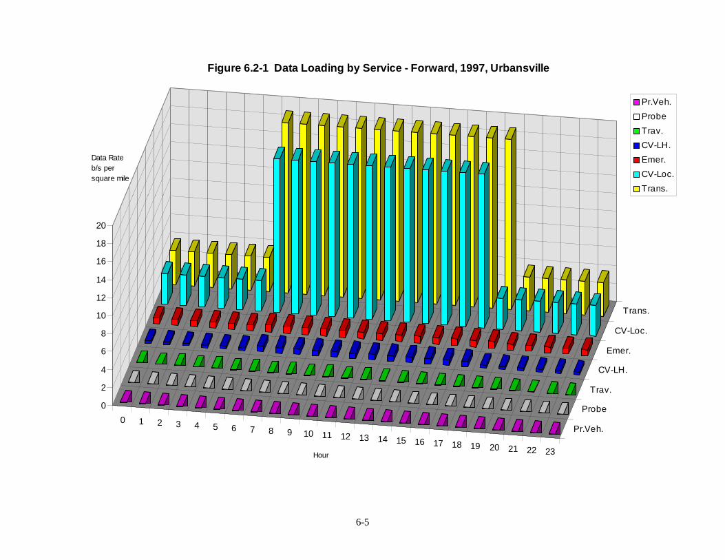
6-5
0 1 2 3 4 5 6 7 8 9 10 11 12 13 14 15 16 17 18 19 20 21 22 23
Pr.Veh.
Probe
T rav.
CV-LH.
E mer.
CV-Loc.
T rans .
0
2
4
6
8
10
12
14
16
18
20
Figure 6.2-1 Data Loading by Service - Forward, 1997, Urbansville
Pr.Veh.
Probe
T rav.
CV-LH.
E mer.
CV-Loc.
T rans .
Data Rateb/s persquare mile
Hour

6-6
0 1 2 3 4 5 6 7 8 9 10 11 12 13 14 15 16 17 18 19 20 21 22 23
T rav.
Pr.Veh.
CV-LH.
E mer.
Probe
T rans .
CV-Loc.
0
1
2
3
4
5
6
7
8
9
Figure 6.2-2 Data Loading by Service - Reverse, 1997, Urbansville
T rav.
Pr.Veh.
CV-LH.
E mer.
Probe
T rans .
CV-Loc.
Data Rateb/s persquare mile
Hour

6-7
0 1 2 3 4 5 6 7 8 9 10 11 12 13 14 15 16 17 18 19 20 21 22 23
R E V
FWD0
5
10
15
20
25
30
35
40
Figure 6.2-3 Total Data Loading, 1997, Urbansv ille.
R E V
FWD
DataRateb/s persquaremile
Hour

6-8
0 1 2 3 4 5 6 7 8 9 10 11 12 13 14 15 16 17 18 19 20 21 22 23
T rav.
Probe
Pr.Veh.
CV-LH.
E mer.
CV-Loc.
T rans .
0
1
2
3
4
5
6
7
Figure 6.2-4 Data Loading by Service - Forward, 1997, Thruville.
T rav.
Probe
Pr.Veh.
CV-LH.
E mer.
CV-Loc.
T rans .
Data Rateb/s persquare mile
Hour

6-9
0 1 2 3 4 5 6 7 8 9 10 11 12 13 14 15 16 17 18 19 20 21 22 23
T rav.
Pr.Veh.
CV-LH.
T rans .
E mer.
Probe
CV-Loc.
0
0.5
1
1.5
2
2.5
3
Figure 6.2-5 Data Loading by Service - Reverse, 1997, Thruville
T rav.
Pr.Veh.
CV-LH.
T rans .
E mer.
Probe
CV-Loc.
Data Rateb/s persquare mile
Hour

6-10
0 1 2 3 4 5 6 7 8 9 10 11 12 13 14 15 16 17 18 19 20 21 22 23
R E V
FWD0
2
4
6
8
10
12
14
Figure 6.2-6 Total Data Loading, 1997, Thruv ille
R E V
FWD
DataRateb/s persquaremile
Hour

6-11
0 1 2 3 4 5 6 7 8 9 10 11 12 13 14 15 16 17 18 19 20 21 22 23
Probe
E mer.
CV-LH.
T rav.
Pr.Veh.
T rans .
CV-Loc.
0
5
10
15
20
25
30
35
40
45
Figure 6.2-7 Data Loading by Service - Forward, 2002, Urbansv ille.
Probe
E mer.
CV-LH.
T rav.
Pr.Veh.
T rans .
CV-Loc.
Data Rateb/s persquare
Hour

6-12
0 1 2 3 4 5 6 7 8 9 10 11 12 13 14 15 16 17 18 19 20 21 22 23
T rav.
CV-LH.
Probe
Pr.Veh.
E mer.
T rans .
CV-Loc.
0
2
4
6
8
10
12
14
16
18
20
Figure 6.2-8 Data Loading by Service - Reverse, 2002, Urbansville.
T rav.
CV-LH.
Probe
Pr.Veh.
E mer.
T rans .
CV-Loc.
Data Rateb/s persquare mile
Hour
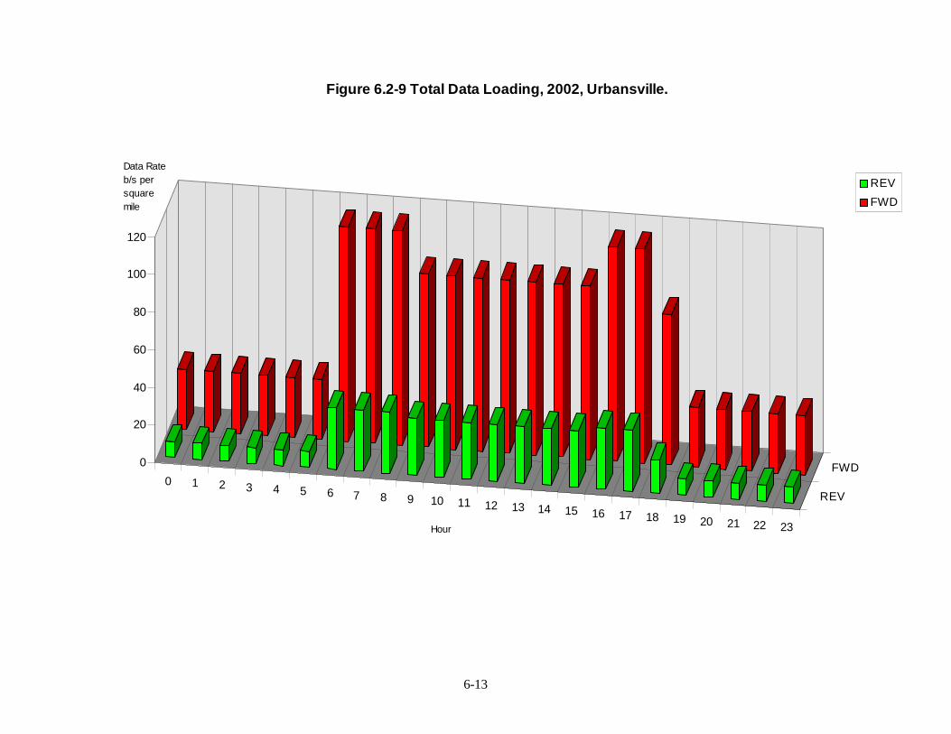
6-13
0 1 2 3 4 5 6 7 8 9 10 11 12 13 14 15 16 17 18 19 20 21 22 23
R E V
FWD0
20
40
60
80
100
120
Figure 6.2-9 Total Data Loading, 2002, Urbansv ille.
R E V
FWD
Data Rateb/s persquaremile
Hour

6-14
0 1 2 3 4 5 6 7 8 9 10 11 12 13 14 15 16 17 18 19 20 21 22 23
Probe
Pr.Veh.
T rav.
CV-LH.
E mer.
T rans .
CV-Loc.
0
2
4
6
8
10
12
14
Figure 6.2-10 Data Loading by Service - Forward, 2002, Thruv ille.
Probe
Pr.Veh.
T rav.
CV-LH.
E mer.
T rans .
CV-Loc.
Data Rateb/s persquare
Hour

6-15
0 1 2 3 4 5 6 7 8 9 10 11 12 13 14 15 16 17 18 19 20 21 22 23
T rav.
CV-LH.
Probe
Pr.Veh.
E mer.
T rans .
CV-Loc.
0
1
2
3
4
5
6
7
Figure 6.2-11 Data Loading by Service - Reverse, 2002, Thruv ille.
T rav.
CV-LH.
Probe
Pr.Veh.
E mer.
T rans .
CV-Loc.
Data Rateb/s persquare mile
Hour

6-16
0 1 2 3 4 5 6 7 8 9 10 11 12 13 14 15 16 17 18 19 20 21 22 23
R E V
FWD0
5
10
15
20
25
30
Figure 6.2-12 Total Data Loading, 2002, Thruv ille
R E V
FWD
Data Rateb/s persquaremile
Hour
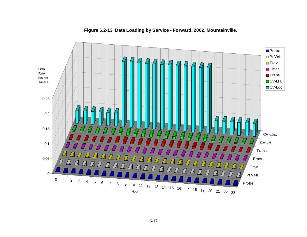
6-17
0 1 2 3 4 5 6 7 8 9 10 11 12 13 14 15 16 17 18 19 20 21 22 23
Probe
Pr.Veh.
T rav.
E mer.
T rans .
CV-LH.
CV-Loc.
0
0.05
0.1
0.15
0.2
0.25
Figure 6.2-13 Data Loading by Service - Forward, 2002, Mountainv ille.
Probe
Pr.Veh.
T rav.
E mer.
T rans .
CV-LH.
CV-Loc.
Data Rateb/s persquare
Hour
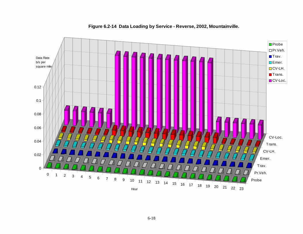
6-18
0 1 2 3 4 5 6 7 8 9 10 11 12 13 14 15 16 17 18 19 20 21 22 23
Probe
Pr.Veh.
T rav.
E mer.
CV-LH.
T rans .
CV-Loc.
0
0.02
0.04
0.06
0.08
0.1
0.12
Figure 6.2-14 Data Loading by Service - Reverse, 2002, Mountainv ille.
Probe
Pr.Veh.
T rav.
E mer.
CV-LH.
T rans .
CV-Loc.
Data Rateb/s persquare mile
Hour

6-19
0 1 2 3 4 5 6 7 8 9 10 11 12 13 14 15 16 17 18 19 20 21 22 23
R E V
FWD0
0.05
0.1
0.15
0.2
0.25
Figure 6.2-15 Total Data Loading, 2002, Mountainv ille.
R E V
FWD
Data Rateb/s persquaremile
Hour

6-20
0 1 2 3 4 5 6 7 8 9 10 11 12 13 14 15 16 17 18 19 20 21 22 23
Probe
E mer.
CV-LH.
T rav.
T rans .
CV-Loc.
Pr.Veh.
0
10
20
30
40
50
60
70
80
90
Figure 6.2-16 Data Loading by Service - Forward, 2012, Urbansv ille.
Probe
E mer.
CV-LH.
T rav.
T rans .
CV-Loc.
Pr.Veh.
Data Rateb/s persquare mile
Hour

6-21
0 1 2 3 4 5 6 7 8 9 10 11 12 13 14 15 16 17 18 19 20 21 22 23
T rav.
CV-LH.
E mer.
Probe
Pr.Veh.
T rans .
CV-Loc.
0
5
10
15
20
25
30
35
40
Figure 6.2-17 Data Loading by Service - Reverse, 2012, Urbansville
T rav.
CV-LH.
E mer.
Probe
Pr.Veh.
T rans .
CV-Loc.
Data Rateb/s persquare mile
Hour

6-22
0 1 2 3 4 5 6 7 8 9 10 11 12 13 14 15 16 17 18 19 20 21 22 23
R E V
FWD0
50
100
150
200
250
Figure 6.2.18 Total Data Loading, 2012, Urbansv ille.
R E V
FWD
Data Rateb/s persquaremile
Hour

6-23
0 1 2 3 4 5 6 7 8 9 10 11 12 13 14 15 16 17 18 19 20 21 22 23
Pr.Veh.
Probe
CV-LH.
E mer.
T rav.
T rans .
CV-Loc.
0
5
10
15
20
25
Figure 6.2-19 Data Loading by Service - Forward, 2012, Thruv ille.
Pr.Veh.
Probe
CV-LH.
E mer.
T rav.
T rans .
CV-Loc.
Data Rateb/s persquare mile
Hour

6-24
0 1 2 3 4 5 6 7 8 9 10 11 12 13 14 15 16 17 18 19 20 21 22 23
T rav.
T rans .
CV-LH.
E mer.
Probe
Pr.Veh.
CV-Loc.
0
2
4
6
8
10
12
Figure 6.2-20 Data Loading by Service - Reverse, 2012, Thruville.
T rav.
T rans .
CV-LH.
E mer.
Probe
Pr.Veh.
CV-Loc.
Data Rateb/s persquare mile
Hour

6-25
0 1 2 3 4 5 6 7 8 9 10 11 12 13 14 15 16 17 18 19 20 21 22 23
R E V
FWD0
5
10
15
20
25
30
35
40
45
Figure 6.2-21 Total Data Loading, 2012, Thruv ille
R E V
FWD
Data Rateb/s persquaremile
Hour

6-26
0 1 2 3 4 5 6 7 8 9 10 11 12 13 14 15 16 17 18 19 20 21 22 23
Probe
E mer.
CV-LH.
T rav.
T rans .
Pr.Veh.
CV-Loc.
0
0.05
0.1
0.15
0.2
0.25
0.3
0.35
0.4
0.45
Figure 6.2-22 Data Loading by Service - Forward, 2012, Mountainv ille.
Probe
E mer.
CV-LH.
T rav.
T rans .
Pr.Veh.
CV-Loc.
Data Rateb/s persquare mile
Hour

6-27
0 1 2 3 4 5 6 7 8 9 10 11 12 13 14 15 16 17 18 19 20 21 22 23
T rav.
E mer.
Probe
CV-LH.
Pr.Veh.
T rans .
CV-Loc.
0
0.02
0.04
0.06
0.08
0.1
0.12
0.14
0.16
0.18
0.2
Figure 6.2-23 Data Loading by Service - Reverse, 2012, Mountainville.
T rav.
E mer.
Probe
CV-LH.
Pr.Veh.
T rans .
CV-Loc.
Data Rateb/s persquare mile
Hour

6-28
0 1 2 3 4 5 6 7 8 9 10 11 12 13 14 15 16 17 18 19 20 21 22 23
REV
FWD0
0.1
0.2
0.3
0.4
0.5
0.6
0.7
0.8
0.9
1
Figure 6.2-24 Total Data Loading, 2012, Mountainville.
REV
FWD
Data Rateb/s persquaremile
Hour

6-29
Table 6.2-1 Summary of Data Loading Results
Units are in bits per second per square mile.No ITS deployment is assumed for Mountainville in 1997.
Year Region Direc. Peak/Off-Peak Pr.Veh. Trav. CV-Loc. CV-LH. Trans. Emer. Probe TOTAL
1997 Urbansville Fwd. Peak per sq. mile: 0.00011 0.001 17.0426 0.61086 18.852 0.8055 0 37.312
1997 Urbansville Fwd. Off-Pk. per sq. mile: 4.6E-05 0.0004 3.40851 0.30543 3.7705 0.6444 0 8.1293
1997 Urbansville Rev. Peak per sq. mile: 0.13586 0.0153 8.40969 0.30144 1.8146 0.6722 1.676 13.025
1997 Urbansville Rev. Off-Pk. per sq. mile: 0.05529 0.0062 1.68194 0.15072 0.3629 0.5377 0.682 3.4768
1997 Thruville Fwd. Peak per sq. mile: 0 0 6.08559 0.2901 6.7306 0.3857 0 13.492
1997 Thruville Fwd. Off-Pk. per sq. mile: 0 0 1.21712 0.14505 1.3461 0.3086 0 3.0168
1997 Thruville Rev. Peak per sq. mile: 0 0 2.99933 0.14247 0.6479 0.3219 0.848 4.9598
1997 Thruville Rev. Off-Pk. per sq. mile: 0 0 0.59987 0.07123 0.1296 0.2575 0.345 1.4034
2002 Urbansville Fwd. Peak per sq. mile: 34.7122 2.0606 41.1999 1.55927 32.765 1.7521 0 114.05
2002 Urbansville Fwd. Off-Pk. per sq. mile: 14.1278 0.8387 8.23998 0.77963 6.553 1.4017 0 31.941
2002 Urbansville Rev. Peak per sq. mile: 1.96875 0.5357 18.6967 0.79403 7.9048 1.4732 1.676 33.049
2002 Urbansville Rev. Off-Pk. per sq. mile: 0.80128 0.218 3.73934 0.39701 1.581 1.1786 0.682 8.5972
2002 Thruville Fwd. Peak per sq. mile: 0.02433 0.48 12.8178 0.64325 11.136 0.8377 0 25.939
2002 Thruville Fwd. Off-Pk. per sq. mile: 0.0099 0.1954 2.56356 0.32162 2.2272 0.6702 0 5.9879
2002 Thruville Rev. Peak per sq. mile: 0.7944 0.0954 6.35185 0.35812 2.6867 0.7044 0.848 11.839
2002 Thruville Rev. Off-Pk. per sq. mile: 0.32332 0.0388 1.27037 0.17906 0.5373 0.5635 0.345 3.2577
2002 Mountainville Fwd. Peak per sq. mile: 4.1E-06 4E-08 0.21779 0.00823 0.0071 0.0025 0 0.2356
2002 Mountainville Fwd. Off-Pk. per sq. mile: 1.7E-06 2E-08 0.04356 0.00412 0.0014 0.002 0 0.0511
2002 Mountainville Rev. Peak per sq. mile: 6.5E-05 5E-07 0.10728 0.00452 0.0086 0.0021 0 0.1226
2002 Mountainville Rev. Off-Pk. per sq. mile: 2.7E-05 2E-07 0.02146 0.00226 0.0017 0.0017 0 0.0272
2012 Urbansville Fwd. Peak per sq. mile: 85.7982 10.484 82.056 3.1208 39.951 2.1606 0 223.57
2012 Urbansville Fwd. Off-Pk. per sq. mile: 34.9199 4.2668 16.4112 1.5604 7.9901 1.7285 0 66.877
2012 Urbansville Rev. Peak per sq. mile: 5.52382 1.7617 36.5907 1.57015 9.6664 1.8167 1.676 58.605
2012 Urbansville Rev. Off-Pk. per sq. mile: 2.24819 0.717 7.31814 0.78508 1.9333 1.4534 0.682 15.137
2012 Thruville Fwd. Peak per sq. mile: 0.11331 3.0041 22.6488 1.14186 12.298 0.9255 0 40.132
2012 Thruville Fwd. Off-Pk. per sq. mile: 0.04612 1.2227 4.52976 0.57093 2.4596 0.7404 0 9.5695
2012 Thruville Rev. Peak per sq. mile: 2.04407 0.2819 11.2614 0.64279 2.9756 0.7782 0.848 18.832
2012 Thruville Rev. Off-Pk. per sq. mile: 0.83194 0.1147 2.25227 0.3214 0.5951 0.6226 0.345 5.0833
2012 Mountainville Fwd. Peak per sq. mile: 0.27402 0.0344 0.40793 0.0156 0.1966 0.0029 0 0.9315
2012 Mountainville Fwd. Off-Pk. per sq. mile: 0.11153 0.014 0.08159 0.0078 0.0393 0.0023 0 0.2566
2012 Mountainville Rev. Peak per sq. mile: 0.01764 0.0058 0.18869 0.00834 0.0476 0.0024 0 0.2705
2012 Mountainville Rev. Off-Pk. per sq. mile: 0.00718 0.0024 0.03774 0.00417 0.0095 0.0019 0 0.0629

6-30
6.2.1.1 Histogram of Message Size DistributionA histogram of the message size distribution for two-way wide area wirless links was prepared for thepeak period for Urbansville for the 2002 time frame. The histogram is shown in Figure 6.2-25. Themessages were sorted by size into bins of generally 100 bits wide, for the forward and reverse directions.The X axis shows the message size bins in units of hundreds of bits, where the “F” prefix is for theforward direction, and the “R” prefix is for the reverse direction. The Y axis shows the number ofmessages in that message size bin for the Urbansville region in the 2002 time frame.
In order to provide a generalized result that can be applied to any urban region for the 2002 time frame,the histogram was calculated on a per-population basis. This histogram can then be used to calculate thedistribution of messages for another urban region by multiplying the results by the population of theregion to be studied. Figure 6.2-26 shows the per-population histogram.

6-31
F,<
1
F,1-
2
F,2-
3
F,3-
4
F,4-
5
F,5-
6
F,6-
8
F,8-
10
F,10
-100
0
R,<
1
R,1
-2
R,2
-3
R,3
-4
R,4
-5
R,5
-6
R,6
-8
R,8
-10
R,1
0-10
00
CV-Loc.T rav.
CV-LH.Pr. Veh.
E mer.Probe
Trans .
0
100000
200000
300000
400000
500000
600000
700000
800000
Figure 6.2-25 Distribution of Messages for Urbansville, 2002, Peak Period
Note:Y-Axis = Number ofmessages in peakperiod;X-Axis = Message (inhundreds of bits);F=Forward Direction;R=Reverse Direction
Figure 6.2-25 Distribution of Messages for Urbansville, 2002, Peak Period

6-32
Figure 6.2-26 Distribution of Messages per Population, Urban Area, 2002, Peak Period
F,<
1
F,1-
2
F,2-
3
F,3-
4
F,4-
5
F,5-
6
F,6-
8
F,8-
10
F,10
-100
0
R,<
1
R,1
-2
R,2
-3
R,3
-4
R,4
-5
R,5
-6
R,6
-8
R,8
-10
R,1
0-10
00
CV-Loc.T rav.
CV-LH.Pr. Veh.
E mer.Probe
Trans .
0
0.05
0.1
0.15
0.2
0.25

6-33
6.2.2 Broadcast Data Loads
Table 6.2-2 lists a set of typical ITS services that are candidates for one-way wirelesscommunication. These include: traffic information, traveler information, and transit services.For each service, the table presents: (1) message name, (2) message length in bits, (3) typicalnumber of required links per geographical area, (4) average update frequency (e.g. traffic dataevery 10 minutes), (5) the effective information rate, which is calculated using the followingexpression:
Information rate (bits/sec) = [Message length (bits/message)]
* [num of traffic links (applicable to the message)]
* [update rate (messages/sec)]
Each message consists of a number of sub-flows. For example, the traffic_data_for_portables iscomposed of:
• tmc_identity• traffic_data_for_media• traveler_identity, current_data_for_media• long_term_data_for_media• predictive_model_data_for_media• long_term_data_for_media• wide_area_pollution_data• pollution_state_area_collection• current_ozone_pollution
Table 6.2-2 presents the size of the messages for a complete set of flows. The update frequencycan be designed so that a full set of data flows for a message is broadcast at a low frequency(e.g., once every 10 minutes) and partial changes are broadcast at a higher frequency (e.g., onceevery minute).
Table 6.2-2 also presents the aggregate information rate. This is the effective information ratethat the communication system must handle to provide these services in a geographical area. Forthese services the aggregate information rate is about 5651 bps.

6-34
Table 6.2-2 Candidate Messages for One Way Wireless Communication
Message Name Size(bits)
No. ofLinks
UpdateFreq.(min.)
Data Rate(bps)
Traffic Information Services
traffic_data_for_portables 819314 1 10 1,366
Aggregate Information Rate (bps) 1,366
Transit Services
transit_deviations_for_portables 3560 1 15 4
traffic_data_for_kiosks 83874939 1 1500 932
transit_deviations_for_kiosks 357648 1 10 596
transit_services_for_portables 2512 1 10 4
Aggregate Information Rate (bps) 1,536
Traveler Information Services
traveler_yellow_pages_data 970 50 10 81
advisory_data 6128 50 5 1,021
broadcast_data 10992 64 10 1,172
link_and_queue_data 400616 4 60 445
yellow_pages_advisory_data 10784 10 60 30
Aggregate Information Rate (bps) 2,750
Total Broadcast Information Rate (bps) 5,651
6.2.3 Short Range DSRC Data Loads
An analysis for DSRC systems when applied to a wide area setting, including data loads, iscontained in Appendix G. The conclusion from there (and elsewhere) is that beacon systems arenot appropriate as a substitute for wide area commercial services for wide area ITS applications(e.g., route guidance). DSRC is only recommended for those specifc applications that require anintimate physical interaction between the vehicle and the roadside infrastructure, such as in tollcollection, commercial vehicle check, roadside safety inspection and the like (see Chapter 3). Inall of these cases, because of the limited coverage of a beacon system and its fairly high data rate,data loading from a capacity standpoint is not an issue.
6.3 Wireline Data Loads
Wireline data loads are less critical than wireless because the current capabilities of the wirelineinfrastructure are simply enormous. Typically, the choice of medium (fiber, coaxial, etc.) isdictated by the desires and budgetary constraints of the jurisdictions. In any event, for

6-35
completeness, wireline data loads based on the subsystem, data flow, and market packagedefinitions have been calculated.
Data loads were calculated for all of the links between subsystems for the wireline (w) interface.Since the frequency of message use on these links is not directly related to usage by individualvehicle end users (for instance, a dataflow performing a database update that is transferring dataon intersection traffic has a size or frequency of use related directly to the number ofintersections in the region), the numerous parameters that enter into this analysis came fromthose used in the teamwork model of the logical architecture and used in sizing there as well.These parameters are all for the 2012 Urbansville scenario, proving a worst-case analysis.
Table 6.3-1 lists the independent parameters assumed in the analysis; Table 6.3-2 shows thederivation of the dependent parameters that are based on the independent parameters.
Table 6.3-1 Independent Parameters Used in the Wireline Data Loading
Name Description Urban 20Year
ADJACENT_TMS The average number of adjacent or cooperating Traffic managementcenters that a TMS within the ITS area under study will communicatewith on a regular basis
5
AHS_MILES The total number of ITS roadway miles being operated under someform of AHS system.
10
AHS_SEGMENT_LENGTH The average length on an AHS segment. 3
AHS_TRIPS_per_DAY The assumed average number of trips each AHS capable vehicle willmake each day.
2
AHS_VEH_per_PLATOON The average size of an AHS platoon, in vehicles. 6
AIR_RATE The proportion of ITS traveler interactions that involve AIR as analternative transportation mode..
0.1
AUTOINFRA The assumed which all ITS users prefer autonomous versusinfrastructure based route guidance.
0.25
BROADCAST_ITEMS The number of broadcast data items typically contained in a specificITS advisory broadcast.
6
COM_VEHS The total number of commercial vehicles operable within the ITS areaunder study.
7802
CONTROLLERS_PER_HIGHWAY_CORRIDOR
The average number of traffic controllers per highway corridor withinthe jurisdiction being studied.
2
CONTROLLERS_PER_ROAD_CORRIDOR
The average number of traffic controllers per road corridor within thejurisdiction being studied.
2
CVI_RATE The rate at which an average Commercial Vehicle Inspector actuallyperforms inspections, expressed as Inspections per second. Thenumbers shown represent an average inspection time ofapproximately 30 minutes, to include preparation, rest periods.
0.0006
CVO_FAC The total number of Commercial Vehicle Roadside facilities that areoperating in the ITS area under study.
1
CVO_FAULT_RATE The assumed rate at which commercial vehicles fail roadsideinspections for all reasons to include safety, permits, drivercredentials etc.
0.01
CVO_MAN The total number of Commercial Vehicle Fleet Managers who canhave simultaneous direct access to ITS at any one time. This will beless than the actual number of such Managers employed within theITS area if they are working shifts.
20
CVO_VEHS The total number of commercial vehicles operable within the ITS areaunder study.
7802
EP_MONITOR_DENSITY The expected number of environmental pollution monitoring points(i.e. roadside transponders) normalized to intersections.
2

6-36
Table 6.3-1 Independent Parameters Used in the Wireline Data Loading
Name Description Urban 20Year
ERMS_CALL_RATE The daily rate at which EMS departments receive calls as a functionof total population. The numbers for the Urban environment are basedon a study of fire department EMS calls in 1994, reported by theJournal of Emergency Medical Services.
0.00034
ERMS_ROUTE_LENGTH The average length of an emergency vehicle route, in miles. 5
ERMS_VEHS The total number of emergency services vehicles available foroperation in the ITS area under study. This takes no account ofwhether the vehicles are active or not.
5981
EVENT_RATE The daily rate at which special events are scheduled which requireITS notifications.
4
FERRY_RATE The proportion of ITS traveler interactions that involve FERRYoperations as an alternative transportation mode..
0.001
HIGHWAY_CORRIDORS The total number of primary highway traffic corridors under ITSstrategic planning and control within the jurisdiction being studied.
18
HIGHWAY_CROSSINGS The total number of controlled or monitored multi-modal crossings ofroads within the ITS environment under study. Based on dataavailable for "typical" urban, interurban and rural areas.
2000
HIGHWAY_MILES Total freeway (limited access ) mileage in the ITS area under study. 225
HIGHWAY_PLAN_SEQUENCES
The number of distinct planned sequences used for highway signactivation..
30
HIGHWAY_SIGN_PLANS The number of distinct plans used for highway sign activation.. 30
HIGHWAY_SIGN_SEQUENCES
The number of distinct sequences used for highway sign activation.. 30
IMAGE_LARGE A large (or high resolution) image, typically used for automatedsurveillance (as opposed to human visual) processes. Roughlyequivalent to a 256 color (or gray scale) image of 1024 X 1024 pictureelements (pels).
1048576
IMAGE_SMALL A small (or low resolution) image, typically used for visualidentification (as opposed to automatic) purposes. Roughly equivalentto a 256 color (or gray scale) image of 640 X 480 picture elements(pels).
307200
INCIDENT_RATE An assumed average incidents per vehicle in a day, normalized togeneral vehicle population (VEHS).
0.0001
INTERSECTIONS The total number of controlled or monitored intersections within theITS environment under study. Based on data available for "typical"urban, interurban and rural areas.
2560
INTERSECTIONS_PER_CORRIDOR
The average number of roadway intersections per corridor within thejurisdiction being studied.
200
JPEG Images are assumed to be compressed for the purposes ofestimating data flow sizes. Still images are assumed to becompressed using the Joint Photographic Experts Group (JPEG)methodology.
0.03
KIOSKS_PER_TRANSIT_STOP
An assumed density of kiosk facilities based on the number of transitstops in the ITS area under study.
0.5
LANE_FLOW_RATE Average traffic flow rate (Vehicles/second) on a single traffic lane.Based on a 24 hour period, this value should be adjusted as requiredto quantify time-of-day and incident specifics.
0.04
LANES_PER_DIRECTION The average number of lanes, in each direction, at an averageintersection.
3
LINK_LENGTH The average length, in miles, of a navigable route link, for the ITSarea under study. This parameter is quantified for roadway links.Pedestrian travelers may require shorter links.
1
LINK_STOPS The average number of stops in an average link. 1

6-37
Table 6.3-1 Independent Parameters Used in the Wireline Data Loading
Name Description Urban 20Year
LINKS_PER_INCIDENT The average number of roadway links affected by an incident. 10
LOCAL_DATA The typical number of data items containing advisory data that will berelevant to the local area surrounding a particular vehicle. Thisparameter is used to "filter" the advisory data list for data loadinganalysis..
3
MAX_AHS_SEGS The maximum allowable number of segments into which a valid ahsroute may be divided. This is an arbitrary assumption and is highlydependent on system design constraints.
10
MAX_ENF_AGENCIES The maximum number of enforcement agencies with which an ITScommunicates.
5
MAX_HIGHWAY_SEGS The maximum allowable number of segments into which a validfreeway route may be divided. This is an arbitrary assumption and ishighly dependent on system design constraints.
10
MAX_ROAD_SEGS The maximum allowable number of segments into which a valid routeover surface streets may be divided. This is an arbitrary assumptionand is highly dependent on system design constraints.
100
MAX_SEG_WPS The maximum allowable number of waypoints which a valid segmentmay utilize. This is an arbitrary assumption and is highly dependenton system design constraints.
10
MAX_STRATEGIES The maximum number of traffic management strategies that can bespecified for use in a single day.
400
MEDIA_OPS The number of Media Operators who can have simultaneous directaccess to the TMC at any one time. This will be less that the actualnumber of Media Operators who actually access the ITS if they areworking shifts.
5
MODE_CHANGES The average number of mode changes in an average traveler route. 1
MOV_BRIDGES The total number of movable bridges within the ITS area under study.Based on available data for typical urban, interurban and rural areas.
4
MP Market penetration assumption for ITS capabilities. It is used where aspecific market penetration (e.g. MP_CVO) is not available orappropriate.
0.5
MP_CVO Market penetration assumption for CVO operations. Expressed as apercentage of the total commercial fleet that will invest in equipmentand/or services to utilize ITS functions.
0.75
MPAHS The assumed AHS Market Penetration, i.e. the percentage ofvehicles that are equipped to operate on AHS lanes.
0.001
MPCV The assumed Commercial Vehicle Market Penetration, i.e. thepercentage of commercial vehicles that are equipped to utilize ITSfunctions.
0.75
MPEG Images are assumed to be compressed for the purposes ofestimating data flow sizes. Full motion images are assumed to becompressed using the Motion Pictures Experts Group (MPEG)methodology. This parameter establishes the ratio assumed in thisanalysis.
0.01
MPKIOSK The market penetration of ITS Travelers using Kiosks. 0.75
MPPDA The market penetration of ITS Travelers using PDA devices. 0.1
MPPTT The assumed Paratransit Traveler Market Penetration, i.e. thepercentage of travelers that utilize paratransit operations.
0.03
MPPTV The assumed Paratransit Vehicle Market Penetration, i.e. thepercentage of vehicles providing flexible transit services that areequipped to utilize ITS functions.
1
MPPV The assumed Private Vehicle Market Penetration, i.e. the percentageof private vehicles that are equipped to utilize ITS functions.
0.1

6-38
Table 6.3-1 Independent Parameters Used in the Wireline Data Loading
Name Description Urban 20Year
MPTR The assumed Traveler Market Penetration, i.e. the percentage oftravelers that will utilize ITS functions.
0.1
MPTU The assumed Transit User Market Penetration, i.e. the percentage oftransit users that utilize ITS functions.
0.15
MPTV The assumed Transit Vehicle Market Penetration, i.e. the percentageof transit vehicles that are equipped to utilize ITS functions.
1
NUM_ROUTES The number of individual routes included in an average trip plan. 6
NUM_SEGS The number of individual route segments included in an averageroute.
10
NUM_TRANSIT_ROUTES The average total number of transit routes included within the ITSenvironment being analyzed. Does not include transit routes of "otherTMS" environments. This is a assumption of a "typical" value derivedfrom demographic data of U.S.
20
PARATRANS_MP Market penetration for paratransit operations. Expressed as apercentage of the total population that will use para-transit facilities.
0.03
PARKING_LANES The maximum number of parking lot payment lanes that are operatingat a single parking lot in the ITS area under study. It is assumed thatthese lanes will only be used by vehicles that are equipped to utilizeITS functions.
2
PARKING_LOTS_PER_PROVIDER
The average total number of parking lots that are being operated by asingle parking lot service provider in the ITS area under study.
4
PARKING_PROVIDER_RATE Number of independent parking providers, normalized to generalvehicle population (VEHS).
0.0002
PARKING_SPACE_RATE Number of independent parking spaces, normalized to generalvehicle population (VEHS).
0.01
PEDESTRIANS The total number of controlled or monitored pedestrian crossings thatare not also intersections within the ITS environment under study.Based on data available for "typical" urban, interurban and ruralareas.
100
POPULATION The total population of the ITS environment under study. 3788627
PTRANSIT_VEHS The total number of Paratransit vehicles operating within the ITS areaunder study. A Paratransit vehicle is one that is used to carry one orpassengers on a non-scheduled transit service that may not follow afixed route.
100
PVT_MP The assumed Private Vehicle Market Penetration, i.e. the percentageof private vehicles that are equipped to utilize ITS functions.
0.1
PVT_VEHS The total number of vehicles excluding commercial and transitvehicles, operable within the ITS area under study.
2273176
RAIL_RATE The proportion of ITS traveler interactions that involve heavy or lightRAIL as an alternative transportation mode..
0.01
RAMPS The total number of controlled or monitored highway access rampswithin the ITS environment under study. Based on data available for"typical" urban, interurban and rural areas.
400
ROAD_ADAPTIVE_PLANS The maximum number of indicator adaptive data (adaptive plans) thatare available from the Manage Traffic Function.
10
ROAD_CORRIDORS The total number of primary road traffic corridors under ITS strategicplanning and control within the jurisdiction being studied.
18
ROAD_CROSSINGS The total number of controlled or monitored multi-modal crossings ofroads within the ITS environment under study. Based on dataavailable for "typical" urban, interurban and rural areas.
2000
ROAD_FIXED_PLANS The maximum number of fixed time indicator control sequences (fixedtime plans) that are available from the Manage Traffic Function.
30

6-39
Table 6.3-1 Independent Parameters Used in the Wireline Data Loading
Name Description Urban 20Year
ROAD_MILES The total mileage of ITS usable roads and streets (as distinct fromhighways) within the area under analysis.
1701
ROUTE_LENGTH The average length (in miles) of the average route requested of, orprovided by the ITS system under study.
15
TAG_DEFECT_RATE The assumed average rate at which tags will be rejected by ITSequipment INCLUDING bad credit, stolen tags and system failures.
0.0001
TOLL_LANES The maximum number of toll lanes that are operating at an averagetoll plaza in the ITS area under study. It is assumed that these laneswill only be used by vehicles that are equipped to utilize ITSfunctions.
2
TOLL_MILES The total number of ITS roadway miles being operated under someform of toll system. Based on available data for typical urban,interurban and rural areas.
50
TOLL_PLAZAS The total number of toll collection points within the ITS area understudy. Based on available data for typical urban, interurban and ruralareas.
10
TRAFFIC_COORDINATION_RULES
The number of road-freeway coordination rules that are available fromthe Manage Traffic Function.
10
TRAFFIC_OPS The number of Traffic Operations Personnel who can havesimultaneous direct access to the TMC at any one time. This will beless than the actual number of Traffic Operations Personnelemployed at the TMC if they are working shifts.
10
TRANSIT_DRIVERS The total number of transit drivers available to operate the transitvehicles within the ITS area under study.
200
TRANSIT_FLEETS The total number of transit fleets operating in the ITS area understudy. The fleets may be operating the same type of service, e.g.buses, or differing types, e.g. one for buses, another for light rail(trams).
3
TRANSIT_STOPS The total number of transit stops on all transit routes within the ITSarea under study. It is assumed that as a minimum, they are allcapable of receiving and displaying data about the next services dueto arrive at the stop.
400
TRANSIT_TECH_WR The average number of transit vehicles that one transit maintenancetechnician can service in an hour.
1
TRANSIT_USAGE_RATE Number of transit users, normalized to total population(POPULATION).
0.01527
TRANSIT_VEHS The total number of transit vehicles available for operation within theITS area under study. A transit vehicle is a special type of vehicle thatis designed and equipped to carry a number of passengers on ascheduled route.
1788
TRANSIT_WAIT_TIME The average waiting time between regularly scheduled transitvehicles.
5
TUNNELS An arbitrary assumption about the number of tunnel segments beingmanaged by the ITS system under study..
1
VEHICLE_SIGN_OUTPUT_DENSITY
The expected number of in-vehicle signage transmission points (i.e.roadside transponders) per intersection.
2
VIDEO_CAMS The total number of video sources in operation within the ITS areaunder study. Video sources are assumed to represent a significantdata communications load.
850
YP_GLOBAL_ITEMS The typical number of items of "yellow pages" type of information thatwill be available from throughout the geographic and/or jurisdictionalarea served by the ITS under study.
15

6-40
Table 6.3-1 Independent Parameters Used in the Wireline Data Loading
Name Description Urban 20Year
YP_LOCAL_ITEMS The typical number of items of "yellow pages" type of information thatwill be available in the local area of a particular vehicle.
15
Table 6.3-2 Dependent Parameters Used in the Wireline Data Loading Analysis
Name Description Basis
ACT_ERMS_VEHS The total number of emergency services vehicles thatare active for any particular emergency call. This willbe a proportion of the total number of emergencyservices vehicles (ERMS_VEHS).
= 0.1 * ERMS_VEHS
AHS_SAMPLE_RATE An arbitrary sample rate constant used to facilitatedata loading estimates for AHS operations.
= 1 / DAY
AHS_VEHS The total number of vehicles that are utilizing AHSfunctions to obtain dynamic in-vehicle route guidance.Based on an assumed market penetration (MPAHS)and the general vehicle population.
= MPAHS * VEHS
AUTONOMOUS_TRAVS The total number of travelers that are utilizingautonomous route guidance. Based on an assumedratio (AUTOINFRA) and the number of guided travelers(ITS_GUIDED_TRAVS).
= AUTOINFRA * ITS_GUIDED_TRAVS
CONTROLLERS The total number of intermodal crossing controllers intraffic corridors.
= HIGHWAY_CROSSING_CONTROLLERS +ROAD_CROSSING_CONTROLLERS
CORRIDORS The total number of traffic corridors. = HIGHWAY_CORRIDORS +ROAD_CORRIDORS
CROSSING_CONTROLLERS
The total number of intermodal crossing controllers intraffic corridors.
= HIGHWAY_CROSSING_CONTROLLERS +ROAD_CROSSING_CONTROLLERS
CROSSINGS The total number of intermodalHIGHWAY_CROSSINGS and ROAD_CROSSINGS
= HIGHWAY_CROSSINGS +ROAD_CROSSINGS
CVC_SAMPLE_RATE An arbitrary sample rate constant used to facilitatedata loading estimates for CVC operations.
= 1 / DAY
CVO_DVR The total number of Commercial Vehicle Drivers whoalso act as their own Fleet Managers. This will be aproportion of the number of Commercial Vehicles(CVO_VEHS). It is assumed that all of the vehiclesbelonging to these owner drivers will be equipped.
=0.5 * CVO_VEHS
CVO_FAC_PER_ROUTE The average number of CVO facilities on a typicalCVO route. Dependent on the assumed total numberof facilities (CVO_FAC) and the relative number ofsegments in a typical route(NUM_SEGS/ROADWAY_SEGS).
= (NUM_SEGS / ROADWAY_SEGS) *CVO_FAC
CVO_INSP The total number of Commercial Vehicle Inspectorswho can have simultaneous direct access to ITS at anyone time in the ITS area under study. This will bedependent on the number of Commercial VehicleRoadside facilities (CVO_FAC).
=2.5 * CVO_FAC

6-41
Table 6.3-2 Dependent Parameters Used in the Wireline Data Loading Analysis
Name Description Basis
DAY Constant used in rate calculations, 24 hours =24 * HOUR
DYNAMIC_TRAVS The total number of travelers that are utilizingautonomous route guidance. Based on an assumedratio (AUTOINFRA) and the number of guided travelers(ITS_GUIDED_TRAVS)
= (1 - AUTOINFRA) * ITS_GUIDED_TRAVS
ERMS_CALLS The rate, in calls per second, at which EMS calls arereceived over an average 24 hour period.
= ERMS_CALL_RATE * (POPULATION) /DAY
GW_SIZE Size of a green wave expressed as a number of routesegments.
= ERMS_ROUTE_LENGTH / LINK_LENGTH
HIGHWAY_CROSSING_CONTROLLERS
The total number of intermodal highway crossingcontrollers in traffic corridors.
= HIGHWAY_CORRIDORS *CONTROLLERS_PER_HIGHWAY_CORRIDOR
HIGHWAY_INDICATORS Total number of indicators (variable message signsand multimodal crossing signals) along freewayscontrolled/monitored within the ITS area under study.Assumed to be proportional to the total freewaymileage.
= HIGHWAY_MILES / 10
HIGHWAY_LINKS The total number of navigable freeway links within theITS area under study.
= HIGHWAY_MILES/LINK_LENGTH
HIGHWAY_SIGN_CONTROLLERS
The total number of highway sign controllers, assumedto be proportional to the number of highway signs.
= 6 * HIGHWAY_SIGNS
HIGHWAY_SIGNS Total number of variable message signs alongfreeways controlled/monitored within the ITS areaunder study. Assumed to be proportional to the totalnumber of freeway ramps.
= RAMPS / 4
HOUR Constant used in rate calculations, 60 minutes =60 * MINUTE
HOV_LANES The total number of high-occupancy links beingcontrolled/monitored within the ITS area under study.Based on the total number of its freeway links.
= .05 * HIGHWAY_LINKS
INCIDENTS The average number of incidents in a 24 hour period,based on the incident rate (INCIDENT_RATE) andgeneral vehicle population (VEHS).
= INCIDENT_RATE * VEHS
INDICATORS Total number of indicators (intersection controllers,pedestrian controllers, variable message signs andmultimodal crossings) controlled/monitored within theITS area under study. Assumed to be proportional tothe number of intersections.
= HIGHWAY_INDICATORS +ROAD_INDICATORS
INT_CONTROLLERS The total number of roadway intersection controllers intraffic corridors.
= CORRIDORS *INTERSECTIONS_PER_CORRIDOR
ITS_CVO_VEHS The total number of commercial vehicles within the ITSarea under study that are equipped to utilize ITSfunctions.
= MPCV * COM_VEHS
ITS_GUIDED_TRAVS The total number of travelers who can utilize ITSpersonal traveler guidance functions. This will be aproportion of the number of travelers who cansimultaneously utilize ITS functions (ITS_TRAVS).
= 0.3 * ITS_TRAVS
ITS_GUIDED_VEHS The total number of vehicles that are utilizing ITSfunctions to obtain dynamic in-vehicle route guidance.This is a subset of the subset of all types of vehiclesequipped to utilize ITS functions (ACT_ERMS_VEHS,ITS_CVO_VEHS, ITS_PVT_VEHS, ITS_PTRANSIT
= ACT_ERMS_VEHS + 0.9 * ITS_CVO_VEHS+ 0.25 * ITS_PVT_VEHS + 0.8 *ITS_PTRANSIT_VEHS + 0.2 *ITS_TRANSIT_VEHS

6-42
Table 6.3-2 Dependent Parameters Used in the Wireline Data Loading Analysis
Name Description Basis
ITS_PARATRANSIT_VEHS The total number of flexible transit vehicles operatingwithin the ITS area under study that are equipped toutilize ITS functions. This will be a proportion of thetotal number of paratransit vehicles(PARATRANSIT_VEHS).
=MPPTV*PARATRANSIT_VEHS
ITS_PTRANSIT_TRAVS The total number of travelers who are utilizing ITSfunctions to obtain information on flexible transitservices and (possibly) make reservation for one ofthose services. This is a proportion of the total numberof travelers who can utilize ITS functions.
= MPPTT*ITS_TRAVS
ITS_PTRANSIT_VEHS The total number of Paratransit vehicles operatingwithin the ITS area under study that are equipped toutilize ITS functions. This will be a proportion of thetotal number of Paratransit vehicles(PTRANSIT_VEHS).
=0.9 * PTRANSIT_VEHS
ITS_PVT_VEHS The total number of private vehicles within the ITSarea under study that are equipped to utilize ITSfunctions.
= MPPV * PVT_VEHS
ITS_RS_TRAVS The total number of travelers who are utilizing ITSfunctions to obtain Ridematching information and(possibly) make Ridematching reservations. This is aproportion of the total number of travelers who canutilize ITS functions (ITS_TRAVS).
= 0.1 * ITS_TRAVS
ITS_TRANSIT_USERS The total number of transit users operating within theITS area under study that utilize ITS functions. This willbe a proportion of the total number of transit users(TRANSIT_USERS).
=MPTU * TRANSIT_USERS
ITS_TRANSIT_VEHS The total number of transit vehicles operating withinthe ITS area under study that are equipped to utilizeITS functions. This will be a proportion of the totalnumber of transit vehicles (TRANSIT_VEHS).
=MPTV * TRANSIT_VEHS
ITS_TRAVS The total number of travelers who can simultaneouslyutilize ITS functions. This is a proportion of the totalpopulation (POPULATION).
= MPTR * POPULATION
ITS_VEHICLES The total number of vehicles within the ITS area understudy that are equipped to utilize ITS functions.
= ACT_ERMS_VEHS + ITS_CVO_VEHS +ITS_PVT_VEHS + ITS_PTRANSIT_VEHS +ITS_TRANSIT_VEHS
KIOSK_EMERGENCIES Number of emergency calls per second beingtransmitted from ITS Kiosks. This assumed to beproportional to the number of ITS travelers(ITS_TRAVS), the expected rate of emergency callswithin the general population (ERMS_CALL_RATE)and the market penetration.
= MPKIOSK * ERMS_CALL_RATE *ITS_TRAVS
LAST_PMODEL_UPDATE This parameter is defined to provide a record of whenthe last time this table was updated. It is the Excel timeserial corresponding to the last time this table wasupdated by PMODEL.XLS
= NOW()
LINKS The total number of navigable links within the ITS areaunder study.
= ROAD_LINKS + HIGHWAY_LINKS
MAX_ADJ_CUR_INCIDENTS
The subset of maximum number of predicted incidentsfor a 24 hour period that will impact traffic conditions inanother area.
= .2 * MAX_CUR_INCIDENTS
MAX_ADJ_PRED_INCIDENTS
The subset of maximum number of predicted incidentsfor a 24 hour period that will impact traffic conditions inanother area.
= .2 * MAX_PRED_INCIDENTS

6-43
Table 6.3-2 Dependent Parameters Used in the Wireline Data Loading Analysis
Name Description Basis
MAX_ADV_CHARGES The maximum number of advanced charges, Assumedto be 1% of the general ITS population, i.e. it isproportional to the general market penetration of ITS(MP).
= .01 * MP * POPULATION
MAX_ADV_FARES The maximum number of advanced fares, Assumed tobe 1% of the general ITS population, i.e. it isproportional to the general market penetration of ITS(MP).
= .01 * MP * POPULATION
MAX_ADV_TOLLS The maximum number of advanced tolls, Assumed tobe 1% of the general ITS population, i.e. it isproportional to the general market penetration of ITS(MP).
= .01 * MP * POPULATION
MAX_AHS_CHECKS The maximum number of AHS check-in/check-outfacilities.
= AHS_MILES / AHS_SEGMENT_LENGTH
MAX_BAD_PAYERS The expected number of travelers who are known tothe ITS system as bad credit risks, assumed to be apercentage of all ITS_TRAVELERS.
= .0001 * ITS_TRAVS
MAX_CUR_INCIDENTS The maximum number of predicted incidents for a 24hour period.
= INCIDENTS
MAX_LINKS The maximum allowable number of segments intowhich a valid route may be divided.
= MAX_SEGS
MAX_PARKING_SENSORS The maximum number of parking lot sensors,Assumed to be proportional to the number ofPARKING_LOTS.
= 10 * PARKING_LOTS
MAX_PARKING_VMS The maximum number of parking variable messagesigns, Assumed to be proportional to the number ofPARKING_LOTS.
= 4 * PARKING_LOTS
MAX_PRED_INCIDENTS The maximum number of predicted incidents for a 24hour period,
= INCIDENTS
MAX_SEGS The total number of navigable links within the ITS areaunder study.
= LINKS
MAX_SENSORS The maximum number of ITS sensors, Assumed to beproportional to the number of intersections in the ITSarea under study.
= 10 * INTERSECTIONS
MILES The total number of miles in the area under study. = HIGHWAY_MILES + ROAD_MILES
MINUTE Constant used in rate calculations, 60 seconds =60
MONTH Constant used in rate calculations, 1/12 of a year =YEAR / 12
NUM_CVO_RECORDS The estimated number of records in the average CVOroadside database. It is based on an estimate of thetotal number of vehicles legally enrolled to operate inthe ITS area under study. This will include all enrolledvehicles registered in the jurisdiction.
=MPCV*CVO_VEHS
NUM_PREDICTED_INCIDENTS
The predicted number of incidents in a 24 hour period. = INCIDENTS
NUM_TRANSIT_SERVICES The maximum number of vehicle schedules for atypical transit route. This is determined theTRANSIT_WAIT_TIME, i.e. an average wait time of 60minutes requires 24 TRANSIT_SERVICES per 24 hourperiod.
= 24 * 60 / TRANSIT_WAIT_TIME
OTHER_SEGS The total number of navigable non-vehicular segmentswithin the ITS area under study.
= .1 * ROAD_LINKS
PARATRANSIT_VEHS The total number of paratransit vehicles operatingwithin the ITS area under study. A paratransit vehicleis one that is used to carry one or passengers on anon-scheduled transit service that may not follow afixed route.
= .25 * TRANSIT_VEHS

6-44
Table 6.3-2 Dependent Parameters Used in the Wireline Data Loading Analysis
Name Description Basis
PARKING_LOT_PROVIDERS
The average number of independent parking serviceproviders in the ITS area under study.
= PARKING_PROVIDER_RATE *POPULATION
PARKING_LOTS The average total number of parking lots that are beingoperated by a single parking lot service provider in theITS area under study.
= PARKING_LOTS_PER_PROVIDER *PARKING_LOT_PROVIDERS
PARKING_SAMPLE_RATE An arbitrary sample rate constant used to facilitatedata loading estimates for parking lot operations.
= 1 / DAY
PARKING_SPACES The total average number of parking spaces availablein the ITS area under study.
= PARKING_SPACE_RATE * VEHS
PED_CONTROLLERS The total number of pedestrian activated signalcontrollers within the ITS area under study. This isdependent on the total number of intersections.
= .1 * INTERSECTIONS
PEDESTRIAN_SIGNAL_CONTROLLERS
The total number of pedestrian activated signalcontrollers within the ITS area under study. This isdependent on the total number of intersections.
= .1 * INTERSECTIONS
PERSONAL_EMERGENCIES
Number of emergency calls per second beingtransmitted from Personal Data Assistant (PDA) typedevices. This assumed to be proportional to thenumber of ITS travelers (ITS_TRAVS), the expectedrate of emergency calls within the general population.
= MPPDA * ERMS_CALL_RATE *ITS_TRAVS
POLLUTION_POINTS The expected number of environmental pollutionmonitoring points (i.e. roadside transponders) . Thisnumber is assumed to be proportional to the number ofintersections (INTERSECTIONS) in the area understudy, and to a installed rate(EP_MONITOR_DENSITY)
= EP_MONITOR_DENSITY *INTERSECTIONS
RAMP_CONTROLLERS The total number of ramp controllers, based on thenumber of ramps, within the ITS area under study.
= 2 * RAMPS
ROAD_CROSSING_CONTROLLERS
The total number of intermodal road crossingcontrollers in traffic corridors.
= ROAD_CORRIDORS *CONTROLLERS_PER_ROAD_CORRIDOR
ROAD_INDICATORS Total number of indicators (intersection controllers,pedestrian controllers, variable message signs andmultimodal crossings) along roadscontrolled/monitored within the ITS area under study.Assumed to be proportional to the number ofintersections.
= 4 * INTERSECTIONS
ROAD_LINKS The total number of navigable surface street linkswithin the ITS area under study.
= ROAD_MILES/LINK_LENGTH
ROAD_SIGN_CONTROLLERS
The total number of road sign controllers, assumed tobe proportional to the number of road signs.
= 6 * ROAD_SIGNS
ROAD_SIGNS Total number of variable message signs along roadscontrolled/monitored within the ITS area under study.Assumed to be proportional to the number ofintersections.
= INTERSECTIONS / 10
ROADWAY_SEGS The total number of navigable route segments withinthe ITS area under study.
= LINKS
ROUTES The average number of routes requested during anaverage 24 hour period, based on the total number ofITS vehicles and travelers within the ITS area understudy.
=2*(ITS_GUIDED_VEHS+ITS_GUIDED_TRAVS)

6-45
Table 6.3-2 Dependent Parameters Used in the Wireline Data Loading Analysis
Name Description Basis
SAMPLE_RATE An arbitrary sample rate constant used to facilitatedata loading estimates.
= 1/(5*MINUTE)
SIGN_CONTROLLERS The total number of roadway sign controllers, assumedto be proportional to the number of signs.
=HIGHWAY_SIGN_CONTROLLERS+ROAD_SIGN_CONTROLLERS
SIGNS The total number of HIGHWAY_SIGNS andROAD_SIGNS
= HIGHWAY_SIGNS+ROAD_SIGNS
TOLL_SAMPLE_RATE An arbitray sample rate constant used to facilitate dataloading estimates for toll road operations.
= 1/DAY
TOLL_SEGS Total number of Toll Segments within the ITS areaunder study. This is a percentage of the number of tollmiles.
= .10 * TOLL_MILES
TOTAL_SEGS The total number of navigable links within the ITS areaunder study.
= LINKS
TRANSIT_DEVS The total number of transit vehicles that are runninglate, i.e. deviating from their routes and/or schedules atany particular moment within the ITS area under study.This will be proportional to the total number of transitvehicles currently running.
= .5 * TRANSIT_VEH_DEVS *TRANSIT_STOPS
TRANSIT_KIOSKS The total number of transit stops within the ITS areaunder study that are also equipped as kiosks and ableto support inquiries from transit users for informationon transit services. This sill be dependent on thenumber of transit stops (TRANSIT_STOPS)
= KIOSKS_PER_TRANSIT_STOP *TRANSIT_STOPS
TRANSIT_ROUTE_SEGS The average (typical) number of route segments in atypical (average) transit route.
= TRANSIT_STOPS /NUM_TRANSIT_ROUTES
TRANSIT_SAMPLE_RATE An arbitrary sample rate constant used to facilitatedata loading estimates for transit operations.
= 1 / DAY
TRANSIT_SEGS The average (typical) number of route segments in atypical (average) transit route.
= TRANSIT_STOPS /NUM_TRANSIT_ROUTES
TRANSIT_TECH_ACTS Transit Technician Activities, assumed to beproportional to the number of TRANSIT_VEHS.
= 2 * TRANSIT_VEHS
TRANSIT_TECHS The total number of transit service techniciansavailable to maintain the transit fleet within the ITSarea under study. This number is assumed to beproportional to the size of the transit system asmeasured by the number of TRANSIT_VEHS
= TRANSIT_VEHS / 50
TRANSIT_USERS The average number of travelers in the generalpopulation (POPULATION) using transit facilities on adaily basis.
= TRANSIT_USAGE_RATE * POPULATION
TRANSIT_VEH_DEVS The total number of transit vehicles that are runninglate, i.e. deviating from their routes and/or schedules atany particular moment within the ITS area under study.This will be proportional to the total number of transitvehicles (TRANSIT_VEHS).
= 0.1 * TRANSIT_VEHS
TRANSIT_VIDEO_CAMS The total number of video sources within the ITS areaunder study that are dedicated to the surveillance oftransit operations. This number is based on the totalnumber of TRANSIT_STOPS in the transit system.
= TRANSIT_STOPS / 8
VEHICLE_SIGN_OUTPUTS The expected number of in-vehicle signagetransmission points (i.e. roadside transponders). Thisnumber is assumed to be proportional to the number ofintersections (INTERSECTIONS) and to the rate ofimplementation(VEHICLE_SIGN_OUTPUT_DENSITY)
= VEHICLE_SIGN_OUTPUT_DENSITY *INTERSECTIONS

6-46
Table 6.3-2 Dependent Parameters Used in the Wireline Data Loading Analysis
Name Description Basis
VEHS The assumed total number of vehicles in the ITS areaunder study, based on the general population of thesame area.
= .63 * POPULATION
WEEK Constant used in rate calculations, 7 days = 7 * DAY
YEAR Constant used in rate calculations, 365.24 days = 365.24 * DAY
The data loads calculated from these parameters can be considered the average data load. Whendetermining the link data load, in addition to this average data load, the latency-driven peak linkloads must be calculated. The maximum of these two (average load and peak link load) was usedto determine the link data rate due to that particular message. The data loads resulting from all ofthe messages that flow over a particular link were summed.
The latencies were all set initially to 0.1 seconds. Where this decision caused a link data rate tobe mainly driven by the latency requirement for a particular large message, the latencyrequirement was adjusted where it was not required to be so low. An example is the transmissionof semi-annual reports where latency is not an issue.
The wireline data loading analysis is shown in Table 6.3-3. The table lists the wireline link in theleft column, the message name, the frequency, the message size, the average link load based onthe frequency and size, the latency requirement assumed, the peak link load based on size andlatency, the maximum of the two load calculations, and finally the type of wireline leased digitallink required to carry this load. As in the wireless analysis section in this document, norecommendation as to the specific link selection has been made. Private fiber networks can bedeployed to carry all or part of this traffic. The selection of a leased digital link type is forillustration only. There are three digital link types assigned in this table: DS0 for up to 56 Kbps,DS1 for up to 1.544 Mbps, and DS3 for over 1.544 Mbps. The largest rate link shown is DS3 (46Mbps), multiple links may be required in some cases. Additionally, it may be less costly to usemultiple lower-rate links and not jump up to the next higher rate link when a threshold isreached. The summary for each link is in bold within a box for each link.

6-47
Table 6.3-3 Wireline Data Loading Analysis, 2012, Urbansville
Wireline Link Message Frequency(/sec)
MessageSize (bits)
Ave. Link Load(b/s)
Latency(sec)
Peak LinkLoad (b/s)
Max. Load(b/s)
LinkType
Construction and Maintenance to TMS fcm_fault_clearance 0.002762541 82 0.226528323 0.1 820 820
Construction and Maintenance to TMS fcm_incident_information 0.002762541 146 0.403330916 0.1 1460 1460
Construction and Maintenance to TMS Total 0.629859239 2280 2280 DS0
CVAS to CVCS cv_credentials_database_update 1.15741E-05 482 0.005578704 0.1 4820 4820
CVAS to CVCS cv_credentials_information_response
0.00015 410 0.0615 0.1 4100 4100
CVAS to CVCS cv_safety_database_update 1.15741E-05 410 0.00474537 0.1 4100 4100
CVAS to CVCS cv_safety_information_response 0.0015 410 0.615 0.1 4100 4100
CVAS to CVCS Total 0.686824074 17120 17120 DS0
CVAS to DMV tdmv_cv_violation_identity_code 1.15741E-05 34 0.000393519 0.1 340 340
CVAS to DMV tdmv_cv_violation_vehicle_license 1.15741E-05 146 0.001689815 0.1 1460 1460
CVAS to DMV Total 0.002083333 1800 1800 DS0
CVAS to Enforcement Agency tea_cv_violation_data 1.15741E-05 274 0.003171296 0.1 2740 2740
CVAS to Enforcement Agency Total 0.003171296 2740 2740 DS0
CVAS to Financial Institution tfi_cv_payment_request 0.08385086 274 22.97513558 0.1 2740 2740

6-48
Table 6.3-3 Wireline Data Loading Analysis, 2012, Urbansville
Wireline Link Message Frequency(/sec)
MessageSize (bits)
Ave. Link Load(b/s)
Latency(sec)
Peak LinkLoad (b/s)
Max. Load(b/s)
LinkType
CVAS to Financial Institution Total 22.97513558 2740 2740 DS0
CVAS to FMS cf_clearance_enrollment_confirm 1.15741E-05 26 0.000300926 0.1 260 260
CVAS to FMS cf_enrollment_information 0.090300926 3818 344.7689352 0.1 38180 38180
CVAS to FMS cf_enrollment_payment_confirmation
0.051600529 170 8.772089947 0.1 1700 1700
CVAS to FMS cv_enrollment_information 0.006450066 3818 24.62635251 0.1 38180 38180
CVAS to FMS cv_enrollment_payment_confirmation
0.025800265 346 8.926891534 0.1 3460 3460
CVAS to FMS Total 387.0945701 81780 81780 DS1
CVAS to Government Administrators tga_quarterly_reports 1.28601E-07 8000018 1.028808899 60 133333.6333 133333.6333
CVAS to Government Administrators tga_request_fees_updates 0.051600529 8000018 412805.1616 10 800001.8 800001.8
CVAS to Government Administrators Total 412806.1904 933335.4333 933335.4333 DS1
CVAS to Other CVAS tocvas_data_table 0.013545139 8210 111.2055903 1 8210 8210
CVAS to Other CVAS tocvas_enrollment_confirmation 0.013545139 82 1.110701389 0.1 820 820
CVAS to Other CVAS tocvas_enrollment_request 0.013545139 50 0.677256944 0.1 500 500
CVAS to Other CVAS tocvas_provide_data 0.013545139 50 0.677256944 0.1 500 500

6-49
Table 6.3-3 Wireline Data Loading Analysis, 2012, Urbansville
Wireline Link Message Frequency(/sec)
MessageSize (bits)
Ave. Link Load(b/s)
Latency(sec)
Peak LinkLoad (b/s)
Max. Load(b/s)
LinkType
CVAS to Other CVAS Total 113.6708056 10030 10030 DS0
CVAS to PS cv_operational_data 1.15741E-05 8192018 94.81502315 10 819201.8 819201.8
CVAS to PS Total 94.81502315 819201.8 819201.8 DS1
CVCS to CVAS cv_credentials_information_request
0.00015 554 0.0831 0.1 5540 5540
CVCS to CVAS cv_roadside_daily_log 1.15741E-05 3362 0.038912037 0.1 33620 33620
CVCS to CVAS cv_safety_information_request 0.0015 554 0.831 0.1 5540 5540
CVCS to CVAS cv_safety_information_request 0.162541667 554 90.04808333 0.1 5540 5540
CVCS to CVAS cv_update_safety_problems_list 0.000015 538 0.00807 0.1 5380 5380
CVCS to CVAS Total 91.00916537 55620 55620 DS0
DMV to CVAS fdmv_cv_violation_state_identity 1.15741E-05 26 0.000300926 0.1 260 260
DMV to CVAS fdmv_cv_violation_vehicle_registration
1.15741E-05 90 0.001041667 0.1 900 900
DMV to CVAS Total 0.001342593 1160 1160 DS0
DMV to PMS fdmv_parking_lot_violation_state_identity
0.000925926 26 0.024074074 0.1 260 260
DMV to PMS fdmv_parking_lot_violation_vehicle_registration
0.000925926 90 0.083333333 0.1 900 900

6-50
Table 6.3-3 Wireline Data Loading Analysis, 2012, Urbansville
Wireline Link Message Frequency(/sec)
MessageSize (bits)
Ave. Link Load(b/s)
Latency(sec)
Peak LinkLoad (b/s)
Max. Load(b/s)
LinkType
DMV to PMS Total 0.107407407 1160 1160 DS0
DMV to TAS fdmv_toll_violation_state_identity 0.000925926 26 0.024074074 0.1 260 260
DMV to TAS fdmv_toll_violation_vehicle_registration
0.000925926 90 0.083333333 0.1 900 900
DMV to TAS Total 0.107407407 1160 1160 DS0
DMV to TMS fdmv_traffic_violation_state_identity
75.93147035 26 1974.218229 0.1 260 1974.218229
DMV to TMS fdmv_traffic_violation_vehicle_registration
75.93147035 90 6833.832332 0.1 900 6833.832332
DMV to TMS Total 8808.050561 1160 8808.050561 DS0
E911 or ETS to EM fets_emergency_telephone_service_identity
0.014908949 146 2.176706531 0.1 1460 1460
E911 or ETS to EM fets_incident_details 0.002762541 202 0.558033185 0.1 2020 2020
E911 or ETS to EM Total 2.734739716 3480 3480 DS0
EM to E911 or ETS tets_incident_acknowledge 0.014908949 26 0.38763267 0.1 260 260
EM to E911 or ETS Total 0.38763267 260 260 DS0
EM to FMS cf_hazmat_request 5.78704E-05 146 0.008449074 0.1 1460 1460
EM to FMS Total 0.008449074 1460 1460 DS0

6-51
Table 6.3-3 Wireline Data Loading Analysis, 2012, Urbansville
Wireline Link Message Frequency(/sec)
MessageSize (bits)
Ave. Link Load(b/s)
Latency(sec)
Peak LinkLoad (b/s)
Max. Load(b/s)
LinkType
EM to ISP emergency_vehicle_route_request 8.917042303 1370 12216.34795 0.1 13700 13700
EM to ISP incident_information 0.001388889 858 1.191666667 0.1 8580 8580
EM to ISP Total 12217.53962 22280 22280 DS0
EM to Other EM toec_emergency_telephone_service_identity
0.014908949 146 2.176706531 0.1 1460 1460
EM to Other EM toec_incident_details 0.014908949 202 3.011607666 0.1 2020 2020
EM to Other EM Total 5.188314197 3480 3480 DS0
EM to PS emergency_vehicle_operational_data
1.15741E-05 819218 9.481689815 15 54614.53333 54614.53333
EM to PS Total 9.481689815 54614.53333 54614.53333 DS0
EM to RTS emergency_request_kiosk_traveler_acknowledge
96.6099885 26 2511.859701 0.1 260 2511.859701
EM to RTS Total 2511.859701 260 2511.859701 DS0
EM to TMS emergency_vehicle_green_wave 8.917042303 1098 9790.912448 0.1 10980 10980
EM to TMS incident_details 0.001388889 218 0.302777778 0.1 2180 2180
EM to TMS incident_response_status 0.003333333 826 2.753333333 0.1 8260 8260
EM to TMS Total 9793.96856 21420 21420 DS0

6-52
Table 6.3-3 Wireline Data Loading Analysis, 2012, Urbansville
Wireline Link Message Frequency(/sec)
MessageSize (bits)
Ave. Link Load(b/s)
Latency(sec)
Peak LinkLoad (b/s)
Max. Load(b/s)
LinkType
EM to TRMS transit_incident_coordination_data 4.62963E-06 41106 0.190305556 0.1 411060 411060
EM to TRMS Total 0.190305556 411060 411060 DS1
EMMS to Map Update Provider tmup_request_pollution_display_update
6.35938E-08 34 2.16219E-06 0.1 340 340
EMMS to Map Update Provider Total 2.16219E-06 340 340 DS0
EMMS to PS pollution_operational_data 1.15741E-05 1843458 21.33631944 100 18434.58 18434.58
EMMS to PS Total 21.33631944 18434.58 18434.58 DS0
EMMS to RS pollution_state_vehicle_acceptance_criteria
0.000277778 642 0.178333333 0.1 6420 6420
EMMS to RS Total 0.178333333 6420 6420 DS0
EMMS to TMS pollution_incident 0.001111111 202 0.224444444 0.1 2020 2020
EMMS to TMS pollution_state_data 0.003333333 282 0.94 0.1 2820 2820
EMMS to TMS wide_area_pollution_data 0.003333333 1024226 3414.086667 30 34140.86667 34140.86667
EMMS to TMS Total 3415.251111 38980.86667 38980.86667 DS0
Event Promoters to TMS fep_event_information 4 530 2120 0.1 5300 5300
Event Promoters to TMS Total 2120 5300 5300 DS0

6-53
Table 6.3-3 Wireline Data Loading Analysis, 2012, Urbansville
Wireline Link Message Frequency(/sec)
MessageSize (bits)
Ave. Link Load(b/s)
Latency(sec)
Peak LinkLoad (b/s)
Max. Load(b/s)
LinkType
Financial Institution to CVAS ffi_cv_payment_confirm 0.067725694 34 2.302673611 0.1 340 340
Financial Institution to CVAS Total 2.302673611 340 340 DS0
Financial Institution to ISP ffi_driver_map_payment_confirm 0.014406915 34 0.489835096 0.1 340 340
Financial Institution to ISP ffi_registration_payment_confirm 0.007203457 34 0.244917548 0.1 340 340
Financial Institution to ISP ffi_traveler_display_payment_confirm
4.384984954 34 149.0894884 0.1 340 340
Financial Institution to ISP ffi_traveler_map_payment_confirm 0.012005763 34 0.408195949 0.1 340 340
Financial Institution to ISP ffi_traveler_other_services_payments_confirm
0.006002882 34 0.204097975 0.1 340 340
Financial Institution to ISP ffi_traveler_rideshare_payment_confirm
0.004322075 34 0.146950542 0.1 340 340
Financial Institution to ISP Total 150.5834855 2040 2040 DS0
Financial Institution to PMS ffi_bad_charges_payment_updates
3.47222E-05 2066 0.071736111 0.1 20660 20660
Financial Institution to PMS ffi_confirm_charges_payment 0.128894326 26 3.351252463 0.1 260 260
Financial Institution to PMS Total 3.422988574 20920 20920 DS0
Financial Institution to TAS ffi_bad_toll_payment_updates 3.47222E-05 2066 0.071736111 0.1 20660 20660
Financial Institution to TAS ffi_confirm_toll_payment 0.128894326 34 4.382407067 0.1 340 340

6-54
Table 6.3-3 Wireline Data Loading Analysis, 2012, Urbansville
Wireline Link Message Frequency(/sec)
MessageSize (bits)
Ave. Link Load(b/s)
Latency(sec)
Peak LinkLoad (b/s)
Max. Load(b/s)
LinkType
Financial Institution to TAS Total 4.454143178 21000 21000 DS0
Financial Institution to TRMS ffi_bad_fare_payment_updates 3.47222E-05 2066 0.071736111 0.1 20660 20660
Financial Institution to TRMS ffi_confirm_fare_payment 0.128894326 26 3.351252463 0.1 260 260
Financial Institution to TRMS ffi_other_services_payment_confirm
0.007203457 34 0.244917548 0.1 340 340
Financial Institution to TRMS Total 3.667906122 21260 21260 DS0
FMS to CVAS cf_enroll_clearance_data 1.15741E-05 402 0.004652778 0.1 4020 4020
FMS to CVAS cf_enrollment_payment_request 0.051600529 414 21.36261905 0.1 4140 4140
FMS to CVAS cf_enrollment_request 0.090300926 3498 315.8726389 0.1 34980 34980
FMS to CVAS cv_enrollment_payment_request 0.045150463 414 18.69229167 0.1 4140 4140
FMS to CVAS cv_enrollment_request 0.006450066 3498 22.56233135 0.1 34980 34980
FMS to CVAS Total 378.4945337 82260 82260 DS1
FMS to EM cf_hazmat_route_information 0.090300926 3754 338.9896759 0.1 37540 37540
FMS to EM cf_hazmat_vehicle_information 1.65344E-06 242 0.000400132 0.1 2420 2420
FMS to EM Total 338.9900761 39960 39960 DS0

6-55
Table 6.3-3 Wireline Data Loading Analysis, 2012, Urbansville
Wireline Link Message Frequency(/sec)
MessageSize (bits)
Ave. Link Load(b/s)
Latency(sec)
Peak LinkLoad (b/s)
Max. Load(b/s)
LinkType
FMS to Intermodal Freight Depot To_Intermodal_Freight_Depot 0.010523964 530 5.577700861 0.1 5300 5300
FMS to Intermodal Freight Depot Total 5.577700861 5300 5300 DS0
FMS to Intermodal Freight Shipper To_Intermodal_Freight_Shipper 0.010523964 530 5.577700861 0.1 5300 5300
FMS to Intermodal Freight Shipper Total 5.577700861 5300 5300 DS0
FMS to ISP cf_route_request 0.090300926 1234 111.4313426 0.1 12340 12340
FMS to ISP cv_route_request 0.045150463 1354 61.13372685 0.1 13540 13540
FMS to ISP Total 172.5650694 25880 25880 DS0
FMS to Payment Instrument tpi_debited_commercial_manager_payment
0.090300926 50 4.515046296 0.1 500 500
FMS to Payment Instrument Total 4.515046296 500 500 DS0
Government Administrators to CVAS fga_carrier_safety_ratings 3.80267E-07 82 3.11819E-05 0.1 820 820
Government Administrators to CVAS fga_tax_and_credential_fees 3.80267E-07 530 0.000201542 0.1 5300 5300
Government Administrators to CVAS Total 0.000232724 6120 6120 DS0
Intermodal Freight Depot to FMS From_Intermodal_Freight_Depot 0.010523964 530 5.577700861 0.1 5300 5300
Intermodal Freight Depot to FMS Total 5.577700861 5300 5300 DS0

6-56
Table 6.3-3 Wireline Data Loading Analysis, 2012, Urbansville
Wireline Link Message Frequency(/sec)
MessageSize (bits)
Ave. Link Load(b/s)
Latency(sec)
Peak LinkLoad (b/s)
Max. Load(b/s)
LinkType
Intermodal Freight Shipper to FMS From_Intermodal_Freight_Shipper 0.010523964 530 5.577700861 0.1 5300 5300
Intermodal Freight Shipper to FMS Total 5.577700861 5300 5300 DS0
Intermodal Transportation Service Provider toISP
fitsp_air_services 37886.27 32768018 >10E+08 10 3276801.8 3276801.8
Intermodal Transportation Service Provider toISP
fitsp_ferry_services 378.8627 32768018 >10E+08 10 3276801.8 3276801.8
Intermodal Transportation Service Provider toISP
fitsp_intermodal_service_confirmation
0.48673333 338 164.5158655 10 33.8 164.5158655
Intermodal Transportation Service Provider toISP
fitsp_rail_services 3788.627 32768018 >10E+08 10 3276801.8 3276801.8
Intermodal Transportation Service Provider to ISP Total 164.5158655 9830439.2 9830569.916 DS3
Intermodal Transportation Service Provider toTRMS
fitsp_transit_service_data 0.000277778 8192018 2275.560556 0.1 81920180 81920180
Intermodal Transportation Service Provider to TRMS Total 2275.560556 81920180 81920180 DS3
ISP to EM emergency_vehicle_route 0.08946 3890 347.9994 0.1 38900 38900
ISP to EM incident_information_request 0.001388889 170 0.236111111 0.1 1700 1700
ISP to EM Total 348.2355111 40600 40600 DS0
ISP to Financial Institution tfi_driver_map_payment_request 0.024003794 274 6.577039641 0.1 2740 2740
ISP to Financial Institution tfi_registration_payment_request 3.80267E-07 274 0.000104193 0.1 2740 2740

6-57
Table 6.3-3 Wireline Data Loading Analysis, 2012, Urbansville
Wireline Link Message Frequency(/sec)
MessageSize (bits)
Ave. Link Load(b/s)
Latency(sec)
Peak LinkLoad (b/s)
Max. Load(b/s)
LinkType
ISP to Financial Institution tfi_traveler_display_payment_request
2.192492477 274 600.7429387 0.1 2740 2740
ISP to Financial Institution tfi_traveler_map_payment_request 0.144069158 274 39.47494942 0.1 2740 2740
ISP to Financial Institution tfi_traveler_other_services_payments_request
0.438498495 274 120.1485877 0.1 2740 2740
ISP to Financial Institution tfi_traveler_rideshare_payment_request
10.52396389 274 2883.566106 0.1 2740 2883.566106
ISP to Financial Institution Total 3650.509725 16440 16583.56611 DS0
ISP to FMS cf_route 0.051600529 3034 156.5560053 0.1 30340 30340
ISP to FMS cv_route 0.045150463 3154 142.4045602 0.1 31540 31540
ISP to FMS Total 298.9605655 61880 61880 DS1
ISP to Intermodal Transportation ServiceProvider
titsp_air_services_request 526.1981944 530 278885.0431 0.1 5300 278885.0431
ISP to Intermodal Transportation ServiceProvider
titsp_confirm_intermodal_service 0.876996991 530 464.8084051 0.1 5300 5300
ISP to Intermodal Transportation ServiceProvider
titsp_ferry_services_request 526.1981944 530 278885.0431 0.1 5300 278885.0431
ISP to Intermodal Transportation ServiceProvider
titsp_rail_services_request 526.1981944 530 278885.0431 0.1 5300 278885.0431
ISP to Intermodal Transportation Service Provider Total 837119.9376 21200 841955.1292 DS1
ISP to Map Update Provider tmup_request_other_routes_map_update
0.016666667 34 0.566666667 0.1 340 340

6-58
Table 6.3-3 Wireline Data Loading Analysis, 2012, Urbansville
Wireline Link Message Frequency(/sec)
MessageSize (bits)
Ave. Link Load(b/s)
Latency(sec)
Peak LinkLoad (b/s)
Max. Load(b/s)
LinkType
ISP to Map Update Provider tmup_request_route_selection_map_update
0.016666667 34 0.566666667 0.1 340 340
ISP to Map Update Provider Total 1.133333333 680 680 DS0
ISP to Media tm_incident_information 0.0000694 819200 56.85248 10 81920 81920
ISP to Media tm_traffic_information 0.001388889 8192018 11377.80278 10 819201.8 819201.8
ISP to Media tm_transit_emergency_information 4.62963E-06 8192018 37.92600926 10 819201.8 819201.8
ISP to Media tm_transit_incident_information 0.60814766 8192018 4981956.575 10 819201.8 4981956.575
ISP to Media tm_transit_schedule_variations 596 2066 1231336 10 206.6 1231336
ISP to Media tm_traveler_information_request 0.001388889 82 0.113888889 10 8.2 8.2
ISP to Media Total 6224765.27 2539740.2 7933624.375 DS3
ISP to Other ISP toisp_data_supply 0.1753429 163840018 28728183.89 5 32768003.6 32768003.6
ISP to Other ISP toisp_request_data 17.53429167 34 596.1659167 0.1 340 596.1659167
ISP to Other ISP Total 28728780.06 32768343.6 32768599.77 DS3
ISP to PMS advanced_other_charges_request 301.3333333 514 154885.3333 0.1 5140 154885.3333
ISP to PMS advanced_traveler_charges_request
0.438498495 370 162.2444433 0.1 3700 3700

6-59
Table 6.3-3 Wireline Data Loading Analysis, 2012, Urbansville
Wireline Link Message Frequency(/sec)
MessageSize (bits)
Ave. Link Load(b/s)
Latency(sec)
Peak LinkLoad (b/s)
Max. Load(b/s)
LinkType
ISP to PMS parking_lot_data_request 52.61981944 34 1789.073861 0.1 340 1789.073861
ISP to PMS parking_lot_reservation_request 0.109624624 34 3.727237211 0.1 340 340
ISP to PMS Total 156840.3789 9520 160714.4072 DS1
ISP to PS current_other_routes_use 0.003333333 34054 113.5133333 1 34054 34054
ISP to PS current_other_routes_use 0.003333333 34054 113.5133333 1 34054 34054
ISP to PS current_road_network_use 0.003333333 385234 1284.113333 1 385234 385234
ISP to PS Total 1511.14 453342 453342 DS1
ISP to RTS advanced_tolls_and_charges_roadside_confirm
298 426 126948 0.1 4260 126948
ISP to RTS traffic_data_for_kiosks 2.192492477 83874957 183895211.5 1 83874956.68 183895211.5
ISP to RTS transit_deviations_for_kiosks 2.192492477 357666 784180.0142 0.1 3576660 3576660
ISP to RTS traveler_payment_confirmation 0.438498495 666 292.0399979 0.1 6660 6660
ISP to RTS traveler_transaction_confirmation 0.438498495 498 218.3722507 0.1 4980 4980
ISP to RTS traveler_trip_information 3.332 33314 111002.248 0.1 333140 333140
ISP to RTS traveler_yellow_pages_data 526.1981944 987.68 519715.4327 0.1 9876.8 519715.4327
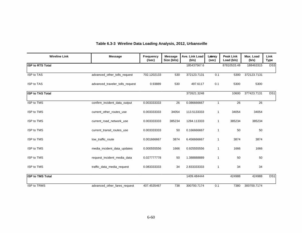
6-60
Table 6.3-3 Wireline Data Loading Analysis, 2012, Urbansville
Wireline Link Message Frequency(/sec)
MessageSize (bits)
Ave. Link Load(b/s)
Latency(sec)
Peak LinkLoad (b/s)
Max. Load(b/s)
LinkType
ISP to RTS Total 185437567.6 87810533.48 188463315 DS3
ISP to TAS advanced_other_tolls_request 702.1202133 530 372123.7131 0.1 5300 372123.7131
ISP to TAS advanced_traveler_tolls_request 0.93889 530 497.6117 0.1 5300 5300
ISP to TAS Total 372621.3248 10600 377423.7131 DS1
ISP to TMS confirm_incident_data_output 0.003333333 26 0.086666667 1 26 26
ISP to TMS current_other_routes_use 0.003333333 34054 113.5133333 1 34054 34054
ISP to TMS current_road_network_use 0.003333333 385234 1284.113333 1 385234 385234
ISP to TMS current_transit_routes_use 0.003333333 50 0.166666667 1 50 50
ISP to TMS low_traffic_route 0.001666667 3874 6.456666667 1 3874 3874
ISP to TMS media_incident_data_updates 0.000555556 1666 0.925555556 1 1666 1666
ISP to TMS request_incident_media_data 0.027777778 50 1.388888889 1 50 50
ISP to TMS traffic_data_media_request 0.083333333 34 2.833333333 1 34 34
ISP to TMS Total 1409.484444 424988 424988 DS1
ISP to TRMS advanced_other_fares_request 407.4535467 738 300700.7174 0.1 7380 300700.7174

6-61
Table 6.3-3 Wireline Data Loading Analysis, 2012, Urbansville
Wireline Link Message Frequency(/sec)
MessageSize (bits)
Ave. Link Load(b/s)
Latency(sec)
Peak LinkLoad (b/s)
Max. Load(b/s)
LinkType
ISP to TRMS advanced_tolls_and_charges_vehicle_confirm
298 426 126948 0.1 4260 126948
ISP to TRMS advanced_traveler_fares_request 0.438498495 738 323.6118896 0.1 7380 7380
ISP to TRMS paratransit_service_confirmation 0.087699699 218 19.1185344 0.1 2180 2180
ISP to TRMS paratransit_trip_request 15.78594583 1418 22384.47119 0.1 14180 22384.47119
ISP to TRMS transit_services_advisories_request
0.003333333 274 0.913333333 0.1 2740 2740
ISP to TRMS transit_services_guidance_request 0.003333333 466 1.553333333 0.1 4660 4660
ISP to TRMS transit_vehicle_deviations_details_request
596 26 15496 0.1 260 15496
ISP to TRMS Total 465874.3857 43040 482489.1886 DS1
ISP to Yellow Pages Service Providers typsp_provider_registration_confirm
3.80267E-07 50 1.90134E-05 0.1 500 500
ISP to Yellow Pages Service Providers typsp_transaction_request 105.2396389 82 8629.650389 0.1 820 8629.650389
ISP to Yellow Pages Service Providers typsp_yellow_pages_info_request 0.003333333 274 0.913333333 0.1 2740 2740
ISP to Yellow Pages Service Providers Total 8630.563741 4060 11869.65039 DS0
Map Update Provider to EMMS fmup_pollution_display_update 0.000277778 16384018 4551.116111 15 1092267.867 1092267.867
Map Update Provider to EMMS Total 4551.116111 1092267.867 1092267.867 DS1

6-62
Table 6.3-3 Wireline Data Loading Analysis, 2012, Urbansville
Wireline Link Message Frequency(/sec)
MessageSize (bits)
Ave. Link Load(b/s)
Latency(sec)
Peak LinkLoad (b/s)
Max. Load(b/s)
LinkType
Map Update Provider to ISP fmup_other_routes_map_data 0.000277778 81920018 22755.56056 5 16384003.6 16384003.6
Map Update Provider to ISP fmup_route_selection_map_data 1.65344E-06 81920018 135.4497652 5 16384003.6 16384003.6
Map Update Provider to ISP Total 22891.01032 32768007.2 32768007.2 DS3
Map Update Provider to PS fmup_deployment_map_update 1.65344E-06 81920018 135.4497652 5 16384003.6 16384003.6
Map Update Provider to PS Total 135.4497652 16384003.6 16384003.6 DS3
Map Update Provider to RTS fmup_traveler_display_update 1.65344E-06 16384018 27.08997685 5 3276803.6 3276803.6
Map Update Provider to RTS Total 27.08997685 3276803.6 3276803.6 DS3
Map Update Provider to TMS fmup_demand_display_update 1.65344E-06 16384018 27.08997685 5 3276803.6 3276803.6
Map Update Provider to TMS fmup_incident_display_update 0.331504863 16384018 5431381.634 5 3276803.6 5431381.634
Map Update Provider to TMS fmup_traffic_display_update 0.001388889 16384018 22755.58056 5 3276803.6 3276803.6
Map Update Provider to TMS Total 5454164.305 9830410.8 11984988.83 DS3
Media to ISP fm_traveler_infirmation 0.000555556 8210 4.561111111 1 8210 8210
Media to ISP Total 4.561111111 8210 8210 DS0
Multimodal Crossings to RS fmmc_crossing_close_duration 1.15741E-05 50 0.000578704 0.1 500 500

6-63
Table 6.3-3 Wireline Data Loading Analysis, 2012, Urbansville
Wireline Link Message Frequency(/sec)
MessageSize (bits)
Ave. Link Load(b/s)
Latency(sec)
Peak LinkLoad (b/s)
Max. Load(b/s)
LinkType
Multimodal Crossings to RS fmmc_crossing_close_time 1.15741E-05 50 0.000578704 0.1 500 500
Multimodal Crossings to RS Total 0.001157407 1000 1000 DS0
Other CVAS to CVAS focvas_data_table 0.013545139 530 7.178923611 0.1 5300 5300
Other CVAS to CVAS focvas_enrollment_confirmation 0.013545139 26 0.352173611 0.1 260 260
Other CVAS to CVAS focvas_enrollment_request 0.013545139 274 3.711368056 0.1 2740 2740
Other CVAS to CVAS focvas_provide_data 0.013545139 66 0.893979167 0.1 660 660
Other CVAS to CVAS Total 12.13644444 8960 8960 DS0
Other EM to EM foec_emergency_telephone_service_identity
0.002762541 146 0.403330916 0.1 1460 1460
Other EM to EM foec_incident_details 0.002762541 202 0.558033185 0.1 2020 2020
Other EM to EM Total 0.961364101 3480 3480 DS0
Other ISP to ISP foisp_data_supply 1.15741E-05 163840018 1896.296505 5 32768003.6 32768003.6
Other ISP to ISP foisp_request_data 0.000277778 34 0.009444444 0.1 340 340
Other ISP to ISP Total 1896.305949 32768343.6 32768343.6 DS3
Other TM to TMS fotc_data_request 1.15741E-05 66 0.000763889 0.1 660 660

6-64
Table 6.3-3 Wireline Data Loading Analysis, 2012, Urbansville
Wireline Link Message Frequency(/sec)
MessageSize (bits)
Ave. Link Load(b/s)
Latency(sec)
Peak LinkLoad (b/s)
Max. Load(b/s)
LinkType
Other TM to TMS fotc_identity 1.15741E-05 50 0.000578704 0.1 500 500
Other TM to TMS fotc_transfer_data 1.15741E-05 4973504.1 57.56370465 5 994700.8164 994700.8164
Other TM to TMS Total 57.56504724 995860.8164 995860.8164 DS1
Other TRM to TRMS fotrm_transit_services 0.001111111 81920018 91022.24222 60 1365333.633 1365333.633
Other TRM to TRMS Total 91022.24222 1365333.633 1365333.633 DS1
Parking Operator to PMS fpo_current_lot_state 0.841917111 50 42.09585556 0.1 500 500
Parking Operator to PMS fpo_lot_occupancy 0.841917111 50 42.09585556 0.1 500 500
Parking Operator to PMS Total 84.19171111 1000 1000 DS0
Parking Service Provider to PMS fpsp_confirm_advanced_parking_payment
0.03507988 26 0.91207687 0.1 260 260
Parking Service Provider to PMS fpsp_current_lot_state 3.367668444 50 168.3834222 0.1 500 500
Parking Service Provider to PMS fpsp_lot_occupancy 3.367668444 50 168.3834222 0.1 500 500
Parking Service Provider to PMS fpsp_parking_lot_charge_change_response
0.03507988 66 2.315272056 0.1 660 660
Parking Service Provider to PMS fpsp_parking_lot_data 0.03507988 146 5.121662426 0.1 1460 1460
Parking Service Provider to PMS fpsp_transaction_reports_request 0.03507988 1042 36.55323457 0.1 10420 10420
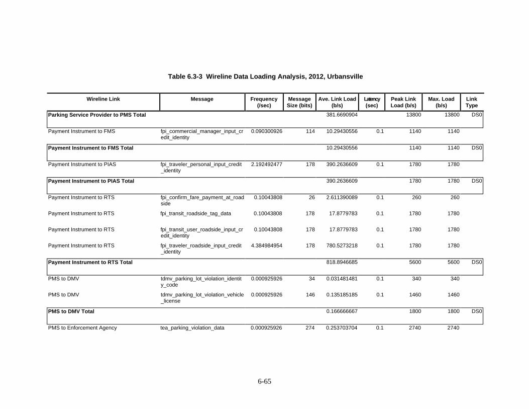
6-65
Table 6.3-3 Wireline Data Loading Analysis, 2012, Urbansville
Wireline Link Message Frequency(/sec)
MessageSize (bits)
Ave. Link Load(b/s)
Latency(sec)
Peak LinkLoad (b/s)
Max. Load(b/s)
LinkType
Parking Service Provider to PMS Total 381.6690904 13800 13800 DS0
Payment Instrument to FMS fpi_commercial_manager_input_credit_identity
0.090300926 114 10.29430556 0.1 1140 1140
Payment Instrument to FMS Total 10.29430556 1140 1140 DS0
Payment Instrument to PIAS fpi_traveler_personal_input_credit_identity
2.192492477 178 390.2636609 0.1 1780 1780
Payment Instrument to PIAS Total 390.2636609 1780 1780 DS0
Payment Instrument to RTS fpi_confirm_fare_payment_at_roadside
0.10043808 26 2.611390089 0.1 260 260
Payment Instrument to RTS fpi_transit_roadside_tag_data 0.10043808 178 17.8779783 0.1 1780 1780
Payment Instrument to RTS fpi_transit_user_roadside_input_credit_identity
0.10043808 178 17.8779783 0.1 1780 1780
Payment Instrument to RTS fpi_traveler_roadside_input_credit_identity
4.384984954 178 780.5273218 0.1 1780 1780
Payment Instrument to RTS Total 818.8946685 5600 5600 DS0
PMS to DMV tdmv_parking_lot_violation_identity_code
0.000925926 34 0.031481481 0.1 340 340
PMS to DMV tdmv_parking_lot_violation_vehicle_license
0.000925926 146 0.135185185 0.1 1460 1460
PMS to DMV Total 0.166666667 1800 1800 DS0
PMS to Enforcement Agency tea_parking_violation_data 0.000925926 274 0.253703704 0.1 2740 2740

6-66
Table 6.3-3 Wireline Data Loading Analysis, 2012, Urbansville
Wireline Link Message Frequency(/sec)
MessageSize (bits)
Ave. Link Load(b/s)
Latency(sec)
Peak LinkLoad (b/s)
Max. Load(b/s)
LinkType
PMS to Enforcement Agency Total 0.253703704 2740 2740 DS0
PMS to Financial Institution tfi_parking_lot_payment_violator_data
0.000185185 2066 0.382592593 0.1 20660 20660
PMS to Financial Institution tfi_request_charges_payment 0.000115741 274 0.031712963 0.1 2740 2740
PMS to Financial Institution Total 0.414305556 23400 23400 DS0
PMS to ISP advanced_other_charges_confirm 108.5729722 346 37566.24839 0.1 3460 37566.24839
PMS to ISP advanced_traveler_charges_confirm
105.2396389 250 26309.90972 0.1 2500 26309.90972
PMS to ISP parking_lot_availability 52.61981944 370 19469.33319 0.1 3700 19469.33319
PMS to ISP parking_lot_reservation_confirm 0.109624624 34 3.727237211 0.1 340 340
PMS to ISP Total 83349.21854 10000 83685.49131 DS1
PMS to Parking Operator tpo_change_lot_state 0.003333333 50 0.166666667 0.1 500 500
PMS to Parking Operator Total 0.166666667 500 500 DS0
PMS to Parking Service Provider tpsp_change_lot_state 0.003333333 82 0.273333333 0.1 820 820
PMS to Parking Service Provider tpsp_parking_lot_charge_change_request
0.001111111 50 0.055555556 0.1 500 500
PMS to Parking Service Provider tpsp_request_advanced_parking_payment
0.2 82 16.4 0.1 820 820

6-67
Table 6.3-3 Wireline Data Loading Analysis, 2012, Urbansville
Wireline Link Message Frequency(/sec)
MessageSize (bits)
Ave. Link Load(b/s)
Latency(sec)
Peak LinkLoad (b/s)
Max. Load(b/s)
LinkType
PMS to Parking Service Provider tpsp_transaction_reports 0.000115741 81920018 9481.483565 100 819200.18 819200.18
PMS to Parking Service Provider Total 9498.212454 821340.18 821340.18 DS1
PMS to TMS parking_lot_charge_change_response
0.001111111 26 0.028888889 0.1 260 260
PMS to TMS parking_lot_current_occupancy 1 170 170 0.1 1700 1700
PMS to TMS parking_lot_current_state 1 178 178 0.1 1780 1780
PMS to TMS vms_parking_guidance_for_highways
1 1947881.4 1947881.405 10 194788.1405 1947881.405
PMS to TMS vms_parking_guidance_for_roads 1 1947881.4 1947881.405 10 194788.1405 1947881.405
PMS to TMS Total 3896110.838 393316.281 3899502.81 DS3
PMS to TRMS parking_lot_price_data 0.000192747 8192018 1578.983546 100 81920.18 81920.18
PMS to TRMS parking_lot_transaction_reports 0.000115741 8192018 948.1502315 100 81920.18 81920.18
PMS to TRMS parking_lot_transit_request 0.005555556 34 0.188888889 0.1 340 340
PMS to TRMS Total 2527.322666 164180.36 164180.36 DS1
PS to Map Update Provider tmup_deployment_map_update_request
1.15741E-05 34 0.000393519 0.1 340 340
PS to Map Update Provider tmup_map_static_data 1.15741E-05 81920018 948.1483565 100 819200.18 819200.18

6-68
Table 6.3-3 Wireline Data Loading Analysis, 2012, Urbansville
Wireline Link Message Frequency(/sec)
MessageSize (bits)
Ave. Link Load(b/s)
Latency(sec)
Peak LinkLoad (b/s)
Max. Load(b/s)
LinkType
PS to Map Update Provider Total 948.14875 819540.18 819540.18 DS1
PS to Transportation Planners ttp_evaluation_results 0.003333333 8192018 27306.72667 100 81920.18 81920.18
PS to Transportation Planners ttp_output_data_store 0.003333333 8192018 27306.72667 100 81920.18 81920.18
PS to Transportation Planners ttp_output_documentation 0.000277778 81920018 22755.56056 100 819200.18 819200.18
PS to Transportation Planners ttp_output_link_data 1.15741E-05 8192018 94.81502315 100 81920.18 81920.18
PS to Transportation Planners ttp_simulation_data 0.003333333 8192018 27306.72667 100 81920.18 81920.18
PS to Transportation Planners Total 104770.5556 1146880.9 1146880.9 DS1
RS to EMMS pollution_state_roadside_collection
1 218 218 0.1 2180 2180
RS to EMMS pollution_state_vehicle_collection 1 178 178 0.1 1780 1780
RS to EMMS pollution_state_vehicle_log_data 0.003333333 178 0.593333333 0.1 1780 1780
RS to EMMS Total 396.5933333 5740 5740 DS0
RS to Multimodal Crossings tmmc_crossing_clear_at_highways
1 50 50 0.1 500 500
RS to Multimodal Crossings tmmc_crossing_clear_at_roads 1 50 50 0.1 500 500
RS to Multimodal Crossings tmmc_stop_alternate_mode_at_highways
1 50 50 0.1 500 500
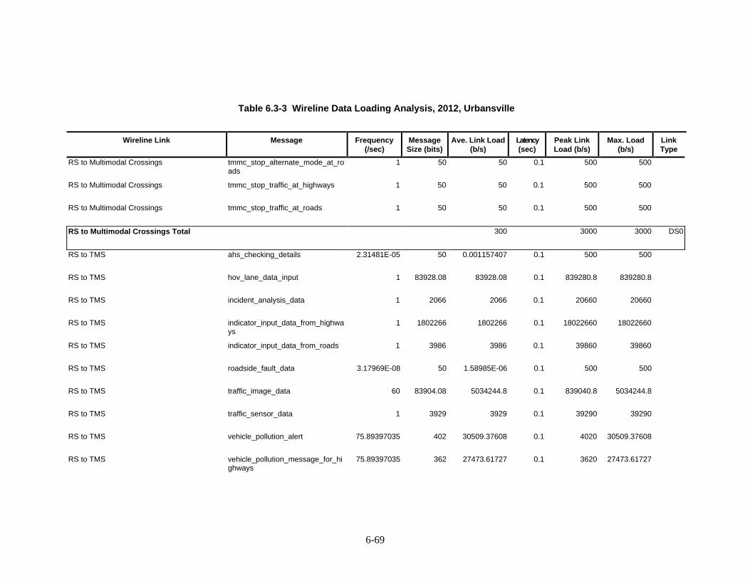
6-69
Table 6.3-3 Wireline Data Loading Analysis, 2012, Urbansville
Wireline Link Message Frequency(/sec)
MessageSize (bits)
Ave. Link Load(b/s)
Latency(sec)
Peak LinkLoad (b/s)
Max. Load(b/s)
LinkType
RS to Multimodal Crossings tmmc_stop_alternate_mode_at_roads
1 50 50 0.1 500 500
RS to Multimodal Crossings tmmc_stop_traffic_at_highways 1 50 50 0.1 500 500
RS to Multimodal Crossings tmmc_stop_traffic_at_roads 1 50 50 0.1 500 500
RS to Multimodal Crossings Total 300 3000 3000 DS0
RS to TMS ahs_checking_details 2.31481E-05 50 0.001157407 0.1 500 500
RS to TMS hov_lane_data_input 1 83928.08 83928.08 0.1 839280.8 839280.8
RS to TMS incident_analysis_data 1 2066 2066 0.1 20660 20660
RS to TMS indicator_input_data_from_highways
1 1802266 1802266 0.1 18022660 18022660
RS to TMS indicator_input_data_from_roads 1 3986 3986 0.1 39860 39860
RS to TMS roadside_fault_data 3.17969E-08 50 1.58985E-06 0.1 500 500
RS to TMS traffic_image_data 60 83904.08 5034244.8 0.1 839040.8 5034244.8
RS to TMS traffic_sensor_data 1 3929 3929 0.1 39290 39290
RS to TMS vehicle_pollution_alert 75.89397035 402 30509.37608 0.1 4020 30509.37608
RS to TMS vehicle_pollution_message_for_highways
75.89397035 362 27473.61727 0.1 3620 27473.61727

6-70
Table 6.3-3 Wireline Data Loading Analysis, 2012, Urbansville
Wireline Link Message Frequency(/sec)
MessageSize (bits)
Ave. Link Load(b/s)
Latency(sec)
Peak LinkLoad (b/s)
Max. Load(b/s)
LinkType
RS to TMS vehicle_pollution_message_for_roads
75.89397035 362 27473.61727 0.1 3620 27473.61727
RS to TMS Total 7015876.492 19813051.6 24082452.21 DS3
RTS to EM emergency_request_kiosk_traveler_details
96.6099885 370 35745.69575 0.1 3700 35745.69575
RTS to EM Total 35745.69575 3700 35745.69575 DS0
RTS to ISP advanced_tolls_and_charges_roadside_request
298 738 219924 0.1 7380 219924
RTS to ISP traffic_data_kiosk_request 2.192492477 98 214.8642627 0.1 980 980
RTS to ISP transit_deviation_kiosk_request 2.192492477 66 144.7045035 0.1 660 660
RTS to ISP traveler_current_condition_request 2.192492477 58 127.1645637 0.1 580 580
RTS to ISP traveler_payment_information 0.438498495 978 428.8515285 0.1 9780 9780
RTS to ISP traveler_transaction_request 0.438498495 402 176.2763951 0.1 4020 4020
RTS to ISP traveler_trip_confirmation 0.438498495 858 376.231709 0.1 8580 8580
RTS to ISP traveler_trip_request 2.192492477 1434 3144.034212 0.1 14340 14340
RTS to ISP traveler_yellow_pages_information_request
2.192492477 26 57.0048044 0.1 260 260
RTS to ISP Total 224593.132 46580 259124 DS1

6-71
Table 6.3-3 Wireline Data Loading Analysis, 2012, Urbansville
Wireline Link Message Frequency(/sec)
MessageSize (bits)
Ave. Link Load(b/s)
Latency(sec)
Peak LinkLoad (b/s)
Max. Load(b/s)
LinkType
RTS to Map Update Provider tmup_request_traveler_display_update
6.35938E-08 34 2.16219E-06 0.1 340 340
RTS to Map Update Provider Total 2.16219E-06 340 340 DS0
RTS to Payment Instrument tpi_debited_fare_payment_at_roadside
0.10043808 50 5.021904018 0.1 500 500
RTS to Payment Instrument tpi_debited_transit_user_payment_at_roadside
0.10043808 50 5.021904018 0.1 500 500
RTS to Payment Instrument tpi_debited_traveler_payment_at_roadside
4.384984954 50 219.2492477 0.1 500 500
RTS to Payment Instrument tpi_request_fare_payment_at_roadside
0.10043808 34 3.414894732 0.1 340 340
RTS to Payment Instrument Total 232.7079505 1840 1840 DS0
RTS to TRMS fare_collection_roadside_violation_information
0.11111 74154 8239.25094 0.1 741540 741540
RTS to TRMS other_services_roadside_request 5.96 2418 14411.28 0.1 24180 24180
RTS to TRMS request_roadside_fare_payment 1788 466 833208 0.1 4660 833208
RTS to TRMS transit_roadside_fare_payment_confirmation
0.10043808 26 2.611390089 0.1 260 260
RTS to TRMS transit_roadside_passenger_data 1.333 122 162.626 0.1 1220 1220
RTS to TRMS transit_services_kiosk_request 2.192492477 314 688.4426377 0.1 3140 3140
RTS to TRMS transit_services_travelers_request 0.13391744 466 62.40552727 0.1 4660 4660

6-72
Table 6.3-3 Wireline Data Loading Analysis, 2012, Urbansville
Wireline Link Message Frequency(/sec)
MessageSize (bits)
Ave. Link Load(b/s)
Latency(sec)
Peak LinkLoad (b/s)
Max. Load(b/s)
LinkType
RTS to TRMS transit_user_roadside_image 3.973788156 73746 293050.9814 0.1 737460 737460
RTS to TRMS Total 1149825.598 1517120 2345668 DS3
Secure Area Environment to TRMS fsa_transit_panic_button 4.62963E-06 50 0.000231481 0.1 500 500
Secure Area Environment to TRMS fsa_transit_video_image 30 8388626 251658780 0.1 83886260 251658780
Secure Area Environment to TRMS Total 251658780 83886760 251659280 DS3
TAS to DMV tdmv_toll_violation_identity_code 0.000925926 34 0.031481481 0.1 340 340
TAS to DMV tdmv_toll_violation_vehicle_license
0.000925926 146 0.135185185 0.1 1460 1460
TAS to DMV Total 0.166666667 1800 1800 DS0
TAS to Enforcement Agency tea_toll_violation_data 0.000925926 274 0.253703704 0.1 2740 2740
TAS to Enforcement Agency Total 0.253703704 2740 2740 DS0
TAS to Financial Institution tfi_request_toll_payment 0.000115741 274 0.031712963 0.1 2740 2740
TAS to Financial Institution tfi_toll_payment_violator_data 0.000185185 2066 0.382592593 0.1 20660 20660
TAS to Financial Institution Total 0.414305556 23400 23400 DS0
TAS to ISP advanced_other_tolls_confirm 509.3598522 346 176238.5089 0.1 3460 176238.5089

6-73
Table 6.3-3 Wireline Data Loading Analysis, 2012, Urbansville
Wireline Link Message Frequency(/sec)
MessageSize (bits)
Ave. Link Load(b/s)
Latency(sec)
Peak LinkLoad (b/s)
Max. Load(b/s)
LinkType
TAS to ISP advanced_traveler_tolls_confirm 105.2396389 250 26309.90972 0.1 2500 26309.90972
TAS to ISP vehicle_toll_probe_data 0.003333333 202 0.673333333 0.1 2020 2020
TAS to ISP Total 202549.0919 7980 204568.4186 DS1
TAS to PS toll_operational_data 1.15741E-05 58.004167 0.000671345 0.1 580.0416667 580.0416667
TAS to PS Total 0.000671345 580.0416667 580.0416667 DS0
TAS to TCS advanced_toll_needed 509.8598522 530 270225.7217 0.1 5300 270225.7217
TAS to TCS toll_bad_payment_check_response
0.666666667 314 209.3333333 0.1 3140 3140
TAS to TCS Total 270435.055 8440 273365.7217 DS1
TAS to TMS probe_data_for_traffic 0.003333333 8210 27.36666667 0.1 82100 82100
TAS to TMS toll_price_changes_response 0.001111111 26 0.028888889 0.1 260 260
TAS to TMS Total 27.39555556 82360 82360 DS1
TAS to Toll Service Provider ttsp_credit_identity 509.8598522 146 74439.53842 0.1 1460 74439.53842
TAS to Toll Service Provider ttsp_toll_price_changes_request 0.001111111 82 0.091111111 0.1 820 820
TAS to Toll Service Provider ttsp_toll_segments 509.8598522 530 270225.7217 0.1 5300 270225.7217

6-74
Table 6.3-3 Wireline Data Loading Analysis, 2012, Urbansville
Wireline Link Message Frequency(/sec)
MessageSize (bits)
Ave. Link Load(b/s)
Latency(sec)
Peak LinkLoad (b/s)
Max. Load(b/s)
LinkType
TAS to Toll Service Provider ttsp_transaction_reports 0.002777778 81920018 227555.6056 20 4096000.9 4096000.9
TAS to Toll Service Provider ttsp_vehicle_identity 509.8598522 274 139701.5995 0.1 2740 139701.5995
TAS to Toll Service Provider Total 711922.5563 4106320.9 4581187.76 DS3
TAS to TRMS toll_price_data 3.81563E-06 914 0.003487485 0.1 9140 9140
TAS to TRMS toll_transaction_reports 0.002777778 8192018 22755.60556 20 409600.9 409600.9
TAS to TRMS Total 22755.60904 418740.9 418740.9 DS1
TCS to TAS advanced_toll_transactions 0.833333333 338 281.6666667 0.1 3380 3380
TCS to TAS confirm_advanced_tolls_payment 0.5 410 205 0.1 4100 4100
TCS to TAS current_toll_transactions 0.666666667 786 524 0.1 7860 7860
TCS to TAS toll_bad_payment_check_request 0.666666667 306 204 0.1 3060 3060
TCS to TAS toll_payment_violator_data 0.000555556 322 0.178888889 0.1 3220 3220
TCS to TAS toll_violation_information 0.000925926 8192018 7585.201852 10 819201.8 819201.8
TCS to TAS Total 8800.047407 840821.8 840821.8 DS1
TMS to Construction and Maintenance tcm_fault_data 0.000235806 82 0.019336081 0.1 820 820

6-75
Table 6.3-3 Wireline Data Loading Analysis, 2012, Urbansville
Wireline Link Message Frequency(/sec)
MessageSize (bits)
Ave. Link Load(b/s)
Latency(sec)
Peak LinkLoad (b/s)
Max. Load(b/s)
LinkType
TMS to Construction and Maintenance tcm_incident_confirmation 0.002762541 26 0.071826054 0.1 260 260
TMS to Construction and Maintenance tcm_request_incident_change 0.002762541 274 0.756936103 0.1 2740 2740
TMS to Construction and Maintenance Total 0.848098237 3820 3820 DS0
TMS to DMV tdmv_traffic_violation_identity_code
75.93147035 34 2581.669992 0.1 340 2581.669992
TMS to DMV tdmv_traffic_violation_vehicle_license
75.93147035 146 11085.99467 0.1 1460 11085.99467
TMS to DMV Total 13667.66466 1800 13667.66466 DS0
TMS to EM incident_alert 0.000277778 842 0.233888889 0.1 8420 8420
TMS to EM incident_details_request 0.001388889 170 0.236111111 0.1 1700 1700
TMS to EM incident_response_clear 0.000277778 146 0.040555556 0.1 1460 1460
TMS to EM Total 0.510555556 11580 11580 DS0
TMS to EMMS pollution_state_data_request 0.003333333 50 0.166666667 0.1 500 500
TMS to EMMS Total 0.166666667 500 500 DS0
TMS to Enforcement Agency tea_traffic_violation_data 75.93147035 274 20805.22288 0.1 2740 20805.22288
TMS to Enforcement Agency Total 20805.22288 2740 20805.22288 DS0

6-76
Table 6.3-3 Wireline Data Loading Analysis, 2012, Urbansville
Wireline Link Message Frequency(/sec)
MessageSize (bits)
Ave. Link Load(b/s)
Latency(sec)
Peak LinkLoad (b/s)
Max. Load(b/s)
LinkType
TMS to Event Promoters tep_event_confirmation 0.000277778 26 0.007222222 0.1 260 260
TMS to Event Promoters Total 0.007222222 260 260 DS0
TMS to ISP current_highway_network_state 0.4 339034 135613.6 0.1 3390340 3390340
TMS to ISP current_road_network_state 0.4 339034 135613.6 0.1 3390340 3390340
TMS to ISP incident_data_output 0.003333333 530 1.766666667 0.1 5300 5300
TMS to ISP link_data_for_guidance 1.15741E-05 578 0.006689815 0.1 5780 5780
TMS to ISP predicted_incidents 0.003333333 194791.74 649.3057894 10 19479.17368 19479.17368
TMS to ISP prediction_data 0.001111111 400634 445.1488889 0.1 4006340 4006340
TMS to ISP retrieved_incident_media_data 0.0055556 90124442 500695.35 10 9012444.2 9012444.2
TMS to ISP traffic_data_for_media 0.083333333 8192018 682668.1667 5 1638403.6 1638403.6
TMS to ISP traffic_data_media_parameters 1.65344E-06 530 0.000876323 0.1 5300 5300
TMS to ISP Total 1455686.946 21473726.97 21473726.97 DS3
TMS to Map Update Provider tmup_request_demand_display_update
6.35938E-08 34 2.16219E-06 0.1 340 340
TMS to Map Update Provider tmup_request_incident_display_update
6.35938E-08 34 2.16219E-06 0.1 340 340

6-77
Table 6.3-3 Wireline Data Loading Analysis, 2012, Urbansville
Wireline Link Message Frequency(/sec)
MessageSize (bits)
Ave. Link Load(b/s)
Latency(sec)
Peak LinkLoad (b/s)
Max. Load(b/s)
LinkType
TMS to Map Update Provider tmup_request_traffic_display_update
1.27188E-07 34 4.32438E-06 0.1 340 340
TMS to Map Update Provider Total 8.64876E-06 1020 1020 DS0
TMS to Other TM totc_data_request 0.003333333 66 0.22 0.1 660 660
TMS to Other TM totc_identity 0.003333333 50 0.166666667 0.1 500 500
TMS to Other TM totc_transfer_data 1.15741E-05 87713260 1015.199769 5 17542652.02 17542652.02
TMS to Other TM Total 1015.586436 17543812.02 17543812.02 DS3
TMS to PMS parking_lot_charge_change_request
0.001111111 322 0.357777778 0.1 3220 3220
TMS to PMS parking_lot_input_data 1 509217.47 509217.4688 10 50921.74688 509217.4688
TMS to PMS selected_parking_lot_control_strategy
0.066666667 436507.83 29100.52203 10 43650.78304 43650.78304
TMS to PMS static_data_for_parking_lots 1.15741E-05 128048 1.482037037 10 12804.8 12804.8
TMS to PMS Total 538319.8306 110597.3299 568893.0518 DS1
TMS to PS ahs_operational_data 1.15741E-05 26.028642 0.000301257 0.1 260.2864198 260.2864198
TMS to PS current_incident_static_data 1.15741E-05 1317104 15.24425926 100 13171.04 13171.04
TMS to PS current_traffic_static_data 1.90781E-07 763847840 145.7279915 100 7638478.4 7638478.4

6-78
Table 6.3-3 Wireline Data Loading Analysis, 2012, Urbansville
Wireline Link Message Frequency(/sec)
MessageSize (bits)
Ave. Link Load(b/s)
Latency(sec)
Peak LinkLoad (b/s)
Max. Load(b/s)
LinkType
TMS to PS traffic_data_for_deployment 1.15741E-05 83874885 970.7741283 10 8387488.468 8387488.468
TMS to PS Total 1131.74668 16039398.19 16039398.19 DS3
TMS to RS ahs_control_data_changes 2.31481E-05 4114 0.095231481 0.1 41140 41140
TMS to RS indicator_control_data_for_highways
1 173674 173674 0.1 1736740 1736740
TMS to RS indicator_control_data_for_roads 1 3561234 3561234 0.1 35612340 35612340
TMS to RS indicator_control_monitoring_data_for_highways
1 173674 173674 0.1 1736740 1736740
TMS to RS indicator_control_monitoring_data_for_roads
1 3561234 3561234 0.1 35612340 35612340
TMS to RS vehicle_sign_data 2 901146 1802292 0.1 9011460 9011460
TMS to RS Total 9272108.095 83750760 83750760 DS3
TMS to TAS toll_price_changes_request 0.001111111 914 1.015555556 0.1 9140 9140
TMS to TAS Total 1.015555556 9140 9140 DS0
TMS to TRMS parking_lot_charge_request 0.003333333 26 0.086666667 0.1 260 260
TMS to TRMS prediction_data 0.001111111 400634 445.1488889 10 40063.4 40063.4
TMS to TRMS toll_price_request 0.003333333 26 0.086666667 0.1 260 260

6-79
Table 6.3-3 Wireline Data Loading Analysis, 2012, Urbansville
Wireline Link Message Frequency(/sec)
MessageSize (bits)
Ave. Link Load(b/s)
Latency(sec)
Peak LinkLoad (b/s)
Max. Load(b/s)
LinkType
TMS to TRMS transit_conditions_demand_request
0.003333333 34 0.113333333 0.1 340 340
TMS to TRMS transit_fare_request 0.003333333 26 0.086666667 0.1 260 260
TMS to TRMS transit_services_changes_request 0.001111111 8210 9.122222222 0.1 82100 82100
TMS to TRMS transit_services_demand_request 0.003333333 562 1.873333333 0.1 5620 5620
TMS to TRMS Total 456.5177778 128903.4 128903.4 DS1
Toll Service Provider to TAS ftsp_confirm_advanced_toll 0.036529774 34 1.242012326 0.1 340 340
Toll Service Provider to TAS ftsp_toll_price_changes_response 3.80267E-07 34 1.29291E-05 0.1 340 340
Toll Service Provider to TAS ftsp_toll_price_data 0.000115741 274 0.031712963 0.1 2740 2740
Toll Service Provider to TAS Total 1.273738218 3420 3420 DS0
Traffic Operations Personnel to EMMS ftop_pollution_data_information_request
0.000277778 50 0.013888889 0.1 500 500
Traffic Operations Personnel to EMMS ftop_pollution_parameter_updates 0.000277778 274 0.076111111 0.1 2740 2740
Traffic Operations Personnel to EMMS Total 0.09 3240 3240 DS0
Transit Maintenance Personnel to TRMS ftmp_transit_vehicle_maintenance_updates
1.15741E-05 530 0.006134259 0.1 5300 5300
Transit Maintenance Personnel to TRMS Total 0.006134259 5300 5300 DS0

6-80
Table 6.3-3 Wireline Data Loading Analysis, 2012, Urbansville
Wireline Link Message Frequency(/sec)
MessageSize (bits)
Ave. Link Load(b/s)
Latency(sec)
Peak LinkLoad (b/s)
Max. Load(b/s)
LinkType
Transit System Operators to TRMS ftso_emergency_request_acknowledge
0.60792 34 20.66928 0.1 340 340
Transit System Operators to TRMS ftso_fare_updates 3.80267E-07 274 0.000104193 0.1 2740 2740
Transit System Operators to TRMS ftso_media_parameter_request 1.15741E-05 34 0.000393519 0.1 340 340
Transit System Operators to TRMS ftso_media_parameter_updates 1.15741E-05 274 0.003171296 0.1 2740 2740
Transit System Operators to TRMS ftso_request_fare_output 3.47222E-05 34 0.001180556 0.1 340 340
Transit System Operators to TRMS ftso_security_action 4.63E-06 146 0.000675922 0.1 1460 1460
Transit System Operators to TRMS Total 20.67480549 7960 7960 DS0
Transportation Planners to PS ftp_evaluation_request 1.15741E-05 146 0.001689815 0.1 1460 1460
Transportation Planners to PS ftp_export_request 1.15741E-05 50 0.000578704 0.1 500 500
Transportation Planners to PS ftp_generation_request 1.15741E-05 2066 0.023912037 0.1 20660 20660
Transportation Planners to PS ftp_import_request 1.15741E-05 82 0.000949074 0.1 820 820
Transportation Planners to PS ftp_output_request 1.15741E-05 82 0.000949074 0.1 820 820
Transportation Planners to PS ftp_parameters 1.15741E-05 274 0.003171296 0.1 2740 2740
Transportation Planners to PS ftp_request_documentation 1.15741E-05 82 0.000949074 0.1 820 820

6-81
Table 6.3-3 Wireline Data Loading Analysis, 2012, Urbansville
Wireline Link Message Frequency(/sec)
MessageSize (bits)
Ave. Link Load(b/s)
Latency(sec)
Peak LinkLoad (b/s)
Max. Load(b/s)
LinkType
Transportation Planners to PS ftp_request_link_data 1.15741E-05 50 0.000578704 0.1 500 500
Transportation Planners to PS ftp_simulation_request 1.15741E-05 34 0.000393519 0.1 340 340
Transportation Planners to PS ftp_static_data 1.15741E-05 530 0.006134259 0.1 5300 5300
Transportation Planners to PS ftp_traffic_data_request 1.15741E-05 34 0.000393519 0.1 340 340
Transportation Planners to PS ftp_update_link_data 1.15741E-05 530 0.006134259 0.1 5300 5300
Transportation Planners to PS Total 0.045833333 39600 39600 DS0
TRMS to EM transit_coordination_data 0.000833333 40994 34.16166667 10 4099.4 4099.4
TRMS to EM transit_emergency_data 0.60814766 178 108.2502834 0.1 1780 1780
TRMS to EM transit_incident_details 4.62963E-06 178 0.000824074 0.1 1780 1780
TRMS to EM Total 142.4127742 7659.4 7659.4 DS0
TRMS to Enforcement Agency tea_fare_collection_roadside_violation_data
178.8 274 48991.2 0.1 2740 48991.2
TRMS to Enforcement Agency tea_fare_collection_vehicle_violation_data
178.8 274 48991.2 0.1 2740 48991.2
TRMS to Enforcement Agency tea_fare_payment_violation_data 3.973788156 274 1088.817955 0.1 2740 2740
TRMS to Enforcement Agency Total 99071.21795 8220 100722.4 DS1

6-82
Table 6.3-3 Wireline Data Loading Analysis, 2012, Urbansville
Wireline Link Message Frequency(/sec)
MessageSize (bits)
Ave. Link Load(b/s)
Latency(sec)
Peak LinkLoad (b/s)
Max. Load(b/s)
LinkType
TRMS to Financial Institution tfi_fare_payment_violator_data 0.496666667 2066 1026.113333 0.1 20660 20660
TRMS to Financial Institution tfi_other_services_payment_request
11.92 274 3266.08 0.1 2740 3266.08
TRMS to Financial Institution tfi_request_fare_payment 1.15741E-05 274 0.003171296 0.1 2740 2740
TRMS to Financial Institution Total 4292.196505 26140 26666.08 DS0
TRMS to Intermodal Transportation ServiceProvider
titsp_transit_arrival_changes 596 4114 2451944 0.1 41140 2451944
TRMS to Intermodal Transportation ServiceProvider
titsp_transit_arrival_deviations 596 4114 2451944 0.1 41140 2451944
TRMS to Intermodal Transportation ServiceProvider
titsp_transit_service_data 0.000277778 8192018 2275.560556 1 8192018 8192018
TRMS to Intermodal Transportation Service Provider Total 4906163.561 8274298 13095906 DS3
TRMS to ISP advanced_other_fares_confirm 407.4535467 410 167055.9541 0.1 4100 167055.9541
TRMS to ISP advanced_tolls_and_charges_vehicle_request
298 738 219924 0.1 7380 219924
TRMS to ISP advanced_traveler_fares_confirm 105.2396389 250 26309.90972 0.1 2500 26309.90972
TRMS to ISP paratransit_personal_schedule 15.78594583 418 6598.525358 0.1 4180 6598.525358
TRMS to ISP transit_deviation_data_received 596 26 15496 0.1 260 15496
TRMS to ISP transit_media_emergency_information
0.60814766 2330 1416.984047 0.1 23300 23300

6-83
Table 6.3-3 Wireline Data Loading Analysis, 2012, Urbansville
Wireline Link Message Frequency(/sec)
MessageSize (bits)
Ave. Link Load(b/s)
Latency(sec)
Peak LinkLoad (b/s)
Max. Load(b/s)
LinkType
TRMS to ISP transit_media_incident_information
4.62963E-06 4378 0.020268519 0.1 43780 43780
TRMS to ISP transit_services_for_advisory_data 0.003333333 172354 574.5133333 0.1 1723540 1723540
TRMS to ISP transit_services_for_guidance 0.003333333 2530 8.433333333 0.1 25300 25300
TRMS to ISP transit_user_payments_transactions
11.92 1042 12420.64 0.1 10420 12420.64
TRMS to ISP transit_vehicle_deviations_details 1.49 398502.8 593769.172 0.1 3985028 3985028
TRMS to ISP Total 1043574.152 5829788 6248753.029 DS3
TRMS to Other TRM totrm_transit_services 0.000277778 81920018 22755.56056 60 1365333.633 1365333.633
TRMS to Other TRM Total 22755.56056 1365333.633 1365333.633 DS1
TRMS to PIAS transit_services_for_portables 2.192492477 2530 5547.005966 0.1 25300 25300
TRMS to PIAS Total 5547.005966 25300 25300 DS0
TRMS to PMS parking_lot_transit_response 0.005555556 34 0.188888889 0.1 340 340
TRMS to PMS Total 0.188888889 340 340 DS0
TRMS to PS financial_reports 1.65344E-06 24577818 40.63792659 60 409630.3 409630.3
TRMS to PS transit_passenger_operational_data
1.15741E-05 26.676481 0.000308756 0.1 266.7648148 266.7648148

6-84
Table 6.3-3 Wireline Data Loading Analysis, 2012, Urbansville
Wireline Link Message Frequency(/sec)
MessageSize (bits)
Ave. Link Load(b/s)
Latency(sec)
Peak LinkLoad (b/s)
Max. Load(b/s)
LinkType
TRMS to PS transit_services_for_deployment 1.15741E-05 172354 1.994837963 1 172354 172354
TRMS to PS Total 42.63307331 582251.0648 582251.0648 DS1
TRMS to RTS confirm_roadside_fare_payment 1788 26 46488 0.1 260 46488
TRMS to RTS other_services_roadside_response
5.96 2418 14411.28 0.1 24180 24180
TRMS to RTS request_transit_user_image 3.973788156 82 325.8506288 0.1 820 820
TRMS to RTS transit_roadside_fare_data 3.80267E-07 922 0.000350607 0.1 9220 9220
TRMS to RTS transit_roadside_fare_payment_debited
1788 26 46488 0.1 260 46488
TRMS to RTS transit_roadside_fare_payment_request
1788 34 60792 0.1 340 60792
TRMS to RTS transit_services_for_kiosks 2.192492477 2378 5213.74711 0.1 23780 23780
TRMS to RTS transit_services_for_roadside_fares
0.000289352 16826 4.868634259 0.1 168260 168260
TRMS to RTS transit_services_for_travelers 0.13391744 2530 338.8111244 0.1 25300 25300
TRMS to RTS transit_vehicle_arrival_time 0.111111111 66 7.333333333 0.1 660 660
TRMS to RTS transit_vehicle_user_data 13.33 106 1412.98 0.1 1060 1412.98
TRMS to RTS Total 175482.8712 254140 407400.98 DS1

6-85
Table 6.3-3 Wireline Data Loading Analysis, 2012, Urbansville
Wireline Link Message Frequency(/sec)
MessageSize (bits)
Ave. Link Load(b/s)
Latency(sec)
Peak LinkLoad (b/s)
Max. Load(b/s)
LinkType
TRMS to Secure Area Environment tsa_broadcast_message 4.62963E-06 402 0.001861111 0.1 4020 4020
TRMS to Secure Area Environment tsa_panuc_button_acknowledge 4.62963E-06 82 0.00037963 0.1 820 820
TRMS to Secure Area Environment Total 0.002240741 4840 4840 DS0
TRMS to TMS parking_lot_charge_details 0.003333333 322 1.073333333 0.1 3220 3220
TRMS to TMS toll_price_details 0.003333333 914 3.046666667 0.1 9140 9140
TRMS to TMS transit_fare_details 0.003333333 17306 57.68666667 0.1 173060 173060
TRMS to TMS transit_highway_overall_priority 596 26 15496 0.1 260 15496
TRMS to TMS transit_ramp_overall_priority 596 146 87016 0.1 1460 87016
TRMS to TMS transit_road_overall_priority 596 26 15496 0.1 260 15496
TRMS to TMS transit_running_data_for_demand 0.003333333 398270.8 1327.569333 1 398270.8 398270.8
TRMS to TMS transit_services_changes_response
0.001111111 34 0.037777778 0.1 340 340
TRMS to TMS transit_services_for_demand 0.003333333 172386 574.62 1 172386 172386
TRMS to TMS Total 119972.0338 758396.8 874424.8 DS1
TRMS to Transit Maintenance Personnel ttmp_work_schedule 0.001241667 8210 10.19408333 0.1 82100 82100

6-86
Table 6.3-3 Wireline Data Loading Analysis, 2012, Urbansville
Wireline Link Message Frequency(/sec)
MessageSize (bits)
Ave. Link Load(b/s)
Latency(sec)
Peak LinkLoad (b/s)
Max. Load(b/s)
LinkType
TRMS to Transit Maintenance Personnel Total 10.19408333 82100 82100 DS1
TRMS to Transit System Operators ttso_emergency_request 0.000833333 530 0.441666667 0.1 5300 5300
TRMS to Transit System Operators ttso_media_parameters 1.15741E-05 8210 0.095023148 0.1 82100 82100
TRMS to Transit System Operators ttso_potential_incidents_alarm 0.000833333 530 0.441666667 0.1 5300 5300
TRMS to Transit System Operators ttso_potential_security_problem 0.000833333 530 0.441666667 0.1 5300 5300
TRMS to Transit System Operators ttso_transaction_reports 1.15741E-05 81920018 948.1483565 100 819200.18 819200.18
TRMS to Transit System Operators ttso_transit_fare_output 3.47222E-05 8210 0.285069444 0.1 82100 82100
TRMS to Transit System Operators Total 949.8534491 999300.18 999300.18 DS1
Weather Service to ISP From_Weather_Service 0.001111111 1042 1.157777778 0.1 10420 10420
Weather Service to ISP fws_current_weather 0.000277778 530 0.147222222 0.1 5300 5300
Weather Service to ISP fws_predicted_weather 0.000277778 530 0.147222222 0.1 5300 5300
Weather Service to ISP Total 1.452222222 21020 21020 DS0
Weather Service to TMS From_Weather_Service 0.001111111 1042 1.157777778 0.1 10420 10420
Weather Service to TMS fws_current_weather 0.000277778 530 0.147222222 0.1 5300 5300

6-87
Table 6.3-3 Wireline Data Loading Analysis, 2012, Urbansville
Wireline Link Message Frequency(/sec)
MessageSize (bits)
Ave. Link Load(b/s)
Latency(sec)
Peak LinkLoad (b/s)
Max. Load(b/s)
LinkType
Weather Service to TMS fws_predicted_weather 0.000277778 530 0.147222222 0.1 5300 5300
Weather Service to TMS Total 1.452222222 21020 21020 DS0
Yellow Pages Service Providers to ISP fypsp_request_provider_registration
3.80267E-07 50 1.90134E-05 0.1 500 500
Yellow Pages Service Providers to ISP fypsp_transaction_confirmation 105.2396389 26 2736.230611 0.1 260 2736.230611
Yellow Pages Service Providers to ISP fypsp_yellow_pages_data 0.003333333 8192018 27306.72667 10 819201.8 819201.8
Yellow Pages Service Providers to ISP Total 30042.9573 819961.8 822438.0306 DS1

6-88
6.4 Analysis of the Data Loading Results
The general trends of the data loads are discussed in this section.
6.4.1 u1t Interface
In 1997 Urbansville, the transit and CVO-local user service groups are the largest users of data inthe forward direction, with the other groups far below. In the reverse direction CVO-local isagain the largest load, with smaller loads from transit and probes groups.
In 1997 Thruville, the transit and CVO-local groups provide the largest loads in the forwarddirection, with the others far below. In the reverse direction CVO-local is alone as the largestload, with probes, transit, and emergency having lower, but significant loads.
In 2002 Urbansville, CVO-local, transit, and private vehicles contribute the largest loads, withthe others far below in the forward direction. In the reverse direction, CVO-local has the highestload with transit about one-half the load. The others are well down.
In 2002 Thruville, CVO-local and transit have the highest loads by a wide margin in the forwarddirection, with CVO-local contributing the largest load in the reverse direction.
In 2002 Mountainville, CVO-local is the largest load with all other users far below it in theforward direction. In the reverse direction CVO-local is alone the largest contributor, with allothers well down.
In 2012 Urbansville, the private vehicles and CVO-local contribute the highest data loads, withtransit at about one-half of their level. The others are well down. In the reverse direction, CVO-local is at the lead again, with transit at about one-third its level with private vehicle a bit lower.
In 2012 Thruville, CVO-local is largest in the forward direction, with transit at about one-half itslevel. In the reverse direction, CVO-local is the largest load with transit next at about one-thirdits level. Private vehicles, probes, and emergency all contribute significant loads.
In 2012 Mountainville, CVO-local has the highest load, with private vehicle and transitsomewhat lower in the forward direction. In the reverse direction, CVO-local has the highestload with transit in second place at about one-fourth its level.
In each of the u1t scenarios and time frames studied, the forward direction data load is alwayshigher than the reverse direction load, by a factor of two to three. The consistent users of thereverse direction are CVO and transit.
6.4.2 u1b Interface
The total aggregate data rate for a single broadcast transmitter sending the entire set of data froma region is 5,651 bps. This rate is easily achieved with any of the second generation broadcastsubcarrier systems (see Section 7). If the data from the region is split between geographically-separated broadcast transmitters, the data rate on any individual transmitter would naturally bereduced.

6-89
6.4.3 u2 Interface
Due to the short propagation range of these systems, which enables fairly high data rates, theirlimited (by definition) coverage, and their layout to cover directly one or more lanes,communication capacity and performance are not issues. Any reasonably well designed multipleaccess scheme would handle the ultiple user within coverage of a given beacon. Variouscommercial solutions are currently available and are deployed in selected locales. There are,however, other issues of technical feasibility if these systems are considered for use to providewide area wireless coverage, through wide spread deployment. These issues are discussed inSection 7 and Appendix G.
6.4.4 u3 Interface
The u3 interface, used for AHS applications, is still in the research stage and is covered inanother program. Since this interface would use very-short-range communications over dedicatedspectrum, there are no ITS communications system design issues that would not be addressedwhile conducting the AHS research independently.
6.4.5 Wireline Interface
There was a total of 140 wireline links studied, including links between subsystems, and to/fromterminators. It was concluded that 60% of these links could be carried over 56 Kbps links. Anadditional 25% of the links could be carried over 1.5 Mbps links. The remaining links haveaggregate data rates as high as 200 Mbps (i.e., for the ISP to RTS, and Secure Area Environmentto TRMS links). In the case of a distributed subsystem, such as RS, the aggregate data load is thetotal load for all elements of the subsystem, where in a distribution network the total aggregateload is seen (such as near the TMS in the RS to TMS link case). Thus, the vast majority of theseremaining links (particularly within a network) can be carried over 45 Mbps links. The wirelineloads determined can easily be carried over numerous existing wireline communications options.

7-1
7. ASSESSMENT OF COMMUNICATION SYSTEMS AND TECHNOLOGIES
7.1 Introduction
In this section, a hot, contentious area is entered, that is, determining which communication systems arebest suited for the ITS applications. It must be established at the outset that the intent of this section isnot to recommend any “winning” systems or technologies – on the contrary, it can be stated a priori thatall so-called winning solutions are at most temporarily such, heroes and victims of an unstoppabletechnology evolution that makes today’s best into tomorrow’s underdogs.
The intent of this section is solely to provide the reader with a characterization of today’s candidatetechnologies that is as complete as possible, and also to offer a glimpse into the systems that loom on thehorizon. Hopefully, this section will provide the implementors with a broad perspective of existingtechnologies. However, this section does not constitute in any way a technology study for any particularscenario. In particular, it does not account for any political, institutional, jurisdictional, budgetary orother similar constraints.
This section contains a broad analysis, review, and assessment of the various communicationtechnologies that are applicable to the ITS architecture. The results of this assessment will lead torecommendations incorporated in the Physical Architecture definition that will be manifested, forexample, in the Architecture Interconnect Specifications (AIS). The analyses herein lead naturally intothe more detailed communication simulation issues addressed in Section 8 which is more focused on thesimulation of a specific wireless system.1
This section begins with the review of the communication analysis objectives and methodology. It thendiscusses the assumptions underlying the systems and technologies selected for analysis – namely the useof shared infrastructure wherever and whenever possible.
1 For practical considerations, the wireless analysis/simulation effort has to be constrained to already standardized open systems.
Since CDPD is the only fully standardized open-system for data communications over cellular (in the U.S. or abroad), with theadded advantage of being already in the deployment stage, it will be analyzed in depth in Section 8 — this does not imply,however, any commitment to CDPD as the ITS wide-area delivery platform.

7-2
7.1.1 Objectives of the Technology Assessment
The main goal of the ITS communication systems technology assessment is to aid in selecting the bestcommunication architecture (framework of system or systems, configurations, technologies, andtechniques) that meet the objectives of the overall ITS system architecture. A secondary objective is toprovide information for the implementors (local DOT’s, etc.) to best match their needs to the capabilitiesof the available systems - subject to specific budgetary constraints.
Through communication systems analysis and a modicum of modeling and simulation, as appropriate, itwill be ascertained how the communications element or "layer" of the system architecture satisfies therequirements at all stages of deployment, especially for the 1997, 2002, and 2012 time frames.
7.1.2 Underlying Assumptions
The strategy for assessing the communication layer of the ITS system architecture reflects both the JointTeam's architecture development philosophy and methodology. The communications layer provides theinformation transfer (data flow) that is required by the transportation layer to implement the desired userservices. This communication component of the architecture must be technically and economicallyfeasible as well as sensitive to the potential institutional and regulatory barriers. To fulfill this vision, thecommunication component has to emerge from current communications infrastructures, and progress in amanner consistent with the predicted evolution of telecommunication systems.
Two main principles will guide the evaluation efforts:
1. Extensive use of available technology whenever and wherever possible, and shared use of emerginginfrastructures in order to minimize the costs directly attributable to ITS; and
2. Monitoring ongoing field trials and tests, as well as other FHWA/Government sponsoredprojects/studies (e.g., AHS Program).
Over the next twenty years, many new communications technologies, from multiple access to transport toswitching, will be introduced at a rapid pace to support the demands of our information age. Thesetechnologies will offer extensive opportunities to handle the ITS user services and should be exploitedfully. The technology projection displayed in Table 7.1-1 identifies the predicted availability of certaincommunication technologies and infrastructures to the year 2012.
In addition to the tremendous financial investment in the existing/emerging communicationinfrastructures (~$20 billion in the cellular infrastructure alone until 1995), an equally large amount oftime and effort has been spent in developing standards to allow inter-operability and inter-connectivityamong these systems. In the process, an extensive practical and theoretical knowledge base has beendeveloped (reviewed in Section 7.5), that greatly expands upon the Phase I Technology Assessment inthe Rockwell Team’s Physical Architecture document. This broad assessment of communicationtechnologies applicable to ITS includes in-depth, quantitative analyses. These analyses will beaugmented in Section 8 with detailed simulations that examine a specific wide area technology deemedwell suited for adoption as a service delivery medium within the National ITS Architecture.
7.1.3 Section Structure
Section 7.2 classifies the communication systems to be assessed into Wireless, both Wide-Area andShort-Range, and Wireline.
Section 7.3 analyzes the impact of non-ITS applications on the ITS service offerings assuming the use ofshared media.

7-3
Section 7.4 analyzes the increasingly important role of protocols and inter-networking issues. It isimportant to understand that in a heterogeneous communications network (that at least encompasses bothwireless and wireline components), it is the inter-networking functions (INF) that guarantee the system’sthroughput.
Section 7.5 presents the Technology Assessment arranged again into wireline and wireless systems, withsubstantially more emphasis on the wireless systems. The latter are classified and analyzed into wirelessmetropolitan area networks (MAN’s), cell-based land-mobile systems, satellite-mobile systems, andbroadcast systems.
Section 7.6 summarizes the Technology Assessment and presents an analysis of the systems side by sideto facilitate comparison. The objective, once again, is not to recommend any specific solution, but tofacilitate the implementors task of selecting the best solution for their identified problems and availablebudgets by having, in a single place, as complete a characterization of the systems as feasible at this time.

7-4
Table 7.1-1 Communications Technology Projections to the Year 2012
Technologies 1992 1997 2002 2012
Wireless Access FDMA
Analog
TDMA/CDMA
Digital
CDMA/TDMA
Digital
CDMA/TDMA
Digital
Wireless Capacity Moderate High (3-5x AMPS) High (5-10x AMPS) High (10-15x AMPS)
Wireless Signal Coverage All Urban, Most Inter-Urban,
Some Rural
All Urban and Inter-Urban,
Most Rural
All Urban and Inter-Urban
All inhabited Rural
Ubiquitous
Wireless Media
• Terrestrial:
• Satellite:
Most Macro
Limited GEO
Full Macro, Initial Micro
Several GEO, Initial LEO
Full Macro, Most Micro
Full GEO, Partial LEO
Transparent, Hybrid Terrestrial Satellite
Integrated Macro/Micro
Full GEO/ Full LEO
Wireline Availability Widespread Copper
Limited Fiber for LAN’s and
Backbone
Fiber Backbone with Copper
Drops
Very Limited Hybrid Fiber-Coax
Very Limited Fiber to Curb
Some Hybrid Fiber-Coax
Partial Fiber to Curb
Limited Fiber to Home
Transfer Mode Full Circuit-Switching
Packet-Switching
Initial Frame-Relaying
Partial Frame-Relaying
Very Limited Asynchronous TransferMode (ATM)
Most Frame-Relaying
Initial Fast-Packet Switching
Partial ATM
Most Fast-Packet Switching
Most ATM
Data Protocol X.25, X.21 Frame-Relay
ATM
Frame-Relay
ATM
Mostly ATM
Transport Network
Characteristics
Service Dependent
Disconnected LAN’s
Slow Speed Interconnection
Initial Service-Independent
Initial LAN Connectivity through
Metropolitan Area Networks (MAN)
Partial Service-Independent
Partial MAN’s
Widespread Service
Integrated Broadband Network—B-ISDN
Most Service Independent
Intelligent Network
Characteristics
Partial Wireline Support:
• Number Translation
Most Wireline Support
Partial Wireless Support
• Mobility Services
(Personal, Terminal)
Full Wireline Support
Most Wireless Support
Fully Integrated Wireline/Wireless Support
• Seamless Operation
• Multi-Mode Terminal
• Profile Portability
• Dynamic Resource Allocation
• Information Format Adaptation

7-5
7.2 Communication Systems Analysis and Assessment Approach
The communication systems/technologies assessment will be presented in two segments – wireless andwireline –reflecting the nature of the communication infrastructure. End-to-end performance, however,warrants looking at the ensemble behavior, not only of the wireless and wireline components of thecommunication layer, but also at the switching/routing elements. It should also be kept in mind, that aswireless systems become more prevalent, some distinctions in use will vanish.
7.2.1 Wireless Communication Systems Analysis
The wireless systems to be considered in an ITS context fall naturally into two different classes having todo with the intended range for information dissemination/collection: wide-area and short-rangecommunication systems.
7.2.1.1 Wide-Area Communication SystemsWireless communication is a broad and rapidly expanding field. The ITS architecture is most concernedwith wireless data communication. Unfortunately, wireless data is a relatively new field, still with anumber of proprietary systems. Moreover, some of the new wireless telecommunications standards thatare being adopted for voice (e.g., CDMA and A-TDMA), have data service proposals that are in theirinfancy. The combination of breadth of communication system possibilities, new technology andproprietary systems, makes the analysis effort a rather daunting task. The analysis will therefore tackledifferent systems/technologies at different levels of depth and detail, ranging from very detailed, state-of-the-art simulation, to cursory quantitative examination of technical information available, even to themore risky anticipation of standards work results. Of course, the systems/technologies that are of mostinterest from a National ITS Architecture standpoint get the most detailed analytical treatment.
The systems to be analyzed are: wireless MAN (Metropolitan Area Network) systems targetingstationary users, land-mobile and satellite-mobile cell-based systems, meteor scatter systems (the “poorman’s” satellite), and broadcast systems. A wide-area beacon-based “solution” is also looked into.
7.2.1.2 Short-Range CommunicationsIn Phase I, Vehicle-to-Vehicle Communications (VtoVC) and Dedicated Short Range Communications(DSRC), were only briefly analyzed. In Phase II, some detail has been added based upon work beingdone in the DSRC area at the standards bodies.
Several subsidized and independent studies are underway in the VtoVC area, some in the U.S. and othersin Europe. A review of the most promising candidates from a national U.S. perspective needs to beperformed. Any ITS architectural implications regarding the adoption of certain solutions should also beidentified. The role of the National ITS Architecture in the definition of VtoVC has been mainly ofmonitoring the progress in the area.
7.2.1.2.1 Dedicated Short Range (formerly Vehicle-to-Roadside) CommunicationsThe applications for which the Dedicated Short Range (DSRC) wireless solution is appropriate havealready been clearly identified in the Physical Architecture document. They include toll collection,parking fee collection, roadside safety inspection, and credentials pre-clearance.
The short range communication systems differ intrinsically from wide area wireless systems such ascellular. The former benefit from being in a confined geographical area (few hundred feet at most), and

7-6
therefore are less susceptible to multi-user, multi-base station interference than systems that cover awhole metropolitan area. The key issues center around the adequacy of the different systems proposed(IR, RF Active, RF Passive) to accommodate the user requirements, and their flexibility andexpandability towards the goal of national compatibility.
7.2.1.2.2 Vehicle-to-Vehicle CommunicationsGiven that AHS is the subject of an ongoing, parallel study that is still in its initial stages, the Joint Teamwill restrict its analysis to a review of proposed interfaces and communication systems, anacknowledgment of the importance of AHS and its impact on the National ITS architecture. Theobjective is to insure inter-operability, especially concerning vehicle-to-vehicle and vehicle-to-roadsidecommunications (VtoVC and DSRC), and that the National ITS Architecture does not inadvertently closeany paths for the AHS Consortium to investigate.
7.2.2 Wireline Communication Analysis
Whereas wireless technologies are quickly evolving in a heated competitive environment, a host ofwireline technologies have become generally accepted, and consequently broadly modeled by a host ofgeneral purpose simulation packages (e.g., OPNET, COMNET, BONES). These wireline technologiesand techniques, however, span a great deal of range in capability, cost, and relative maturity (e.g., fiberversus coaxial versus twisted-pair; ISDN versus frame relay versus FDDI versus ATM). The wirelineinfrastructure to support ITS applications can, therefore, be an arena of much selection and variabilitydepending on the disparate transportation needs, objectives, and budget of the many jurisdictions.
In Phase I, it was concluded that the wireline portion of the communication systems supporting ITS willnot constitute the communications bottleneck. (The Phase I wireline simulation results are included inSection 8 for the reader’s convenience.) In fact, through proper design, and given the many alternativesavailable, the capacity and/or throughput of wireline systems can be made to meet the users’requirements (with any desired margins) satisfying any least cost criterion. Thus, the emphasis in Phase IIis on communication systems and protocols that could not be analyzed in Phase I due to lack of resourcesand because models were not available.
7.2.3 End-to-End Communication Analysis
The above separate analysis of the wireline and wireless components of the communicationsinfrastructure needs to be combined with the objective of assessing the end-to-end system performance.Referring back to Figure 3.2-3 depicting the AID-level 0, end-to-end performance from an ITS serviceperspective can be viewed as comprising: 1.) communication system performance (wireless and wirelinesegments connecting two AID subsystems as well as the switching/routing elements), and 2.) theperformance of the “transportation layer” subsystems themselves (their processing time, any data baseaccess time, etc.). The overall end-to-end ITS service requirements are elucidated in the MissionDefinition document and are derived, in many cases, from inexact human factors related to ITS serviceacceptance.
Since the performance of any ITS subsystem is a moving target, driven primarily be the stakeholders’budgetary constraints, the focus here and in Section 8 will be only on the telecommunication segment(wireless and wireline). In the end, it will be seen that the communication layer implementationsconsidered will not place any undue constraint or limitation on the provision of the ITS services.

7-7
7.3 Non-ITS Applications and Their Impact
When obtaining the communication systems’ end-to-end performance for any deployed infrastructurewith other users, it is intuitive that the traffic generated by non-ITS users will have an impact on the ITSperformance.
To illustrate, we use CDPD here as an example. If the ITS data loads can be accommodated on oneCDPD channel per sector (the so called minimal deployment even out to 20 years), and if the non-ITStraffic is a few times that of ITS, the total traffic may not be accommodated on only one channel.
On the other hand, the crux, as well as the advantage of cell based systems, is that the solution for thehigher traffic is simply to deploy more (in this case CDPD) channels as needed. (Loaded data channelsare more profitable than voice to the carrier.) In fact, the voice demand leads the way to the deploymentof new cells and splitting the present cells into smaller and smaller ones, that continue to have more orless the same load. CDPD deployment (as that of any other overlay system) follows that of voice.2
The difficulty in assessing the effect of non-ITS users resides in the characterization of the traffic theygenerate. After long discussions both inside the Team and with wireless data experts in variouscompanies, it was agreed that a few non-ITS applications are “promising”:
1) Credit Card/Transaction Authorization and Fixed/Mobile POS
• Taxis
• Food Delivery
• Door-to-Door Sales
• Landscaping, Pool care, Snow Removal, etc.
• Gas Stations
• Fast Food
• Other Retail
2) Telemetry
• Oil, gas, water and power monitoring
• Oil, gas and water well production monitoring and control
• Oil and gas pipeline monitoring and control
• Electric power demand monitoring
• Storage tank level monitoring
• Pollution and noise level monitoring
• Vending machine remote inventory control and loss management
3) Field Service (Appliances, Cable, Utilities, High Tech, Office Equipment)
• Job dispatch
• Information access
• Reporting
4) Health Care (Visiting Nurses, House Calls)
2 In Phase I, an analysis was made regarding the case of one reserved CDPD channel plus another one dynamically assigned as a
function of availability and demand. In Phase II the case was considered of one reserved CDPD channel, as well as a totallydynamic solution for the CDPD problem with no reserved channels.

7-8
• Job dispatch
• Information access
• Reporting
5) Field Sale
• Catalog/Information access
• Order placing
6) Public Safety
• NCIC inquiry
• State and Local data base access
• Incident and shift reporting
7) Security
• Keycard access
• Commercial Alarms
8) Mobile Office
• LAN access: File synchronization, file transfer, data base access, calendar update, etc.
• Internet access
9) Remote Access
• Internet access
Looking at the above list, which does not presume to cover all the upcoming uses of wireless data access,two distinct classes of applications can be observed: one corresponding to occasional, burstytransactions, including all entries 1) to 7), and another corresponding to a more or less continuous use ofthe system, with longer “transactions”, constituting a traffic background for the first class of applications.
At this point, in order to get some feeling for the non-ITS traffic to be expected, it becomes necessary topredict the number of users in each category. This is obviously the subject of much heated debate withpredictions covering the whole spectrum, depending on how optimistic, realistic, or pessimistic theauthors want to be.
Based upon Market Research information GTE obtained from a few, well respected companies, and someinternal market projections, the numbers of wireless data users for the year 2002, shown in Table 7.3-1and Figure 7.3-1, were settled upon. Those figures are nothing more than just another projection. It willlater be shown however, that it is a rather sensible projection.
7.3.1 Non-ITS Wireless Data Market Projections for 2002
A slightly different classification will be used in coming up with projections for the number of users foreach type of applications.

7-9
Table 7.3-1 Wireless Data Market Projections (from External and GTE Market Studies)
Number of Wireless Data Users (x1000) 1994 1995 1996 1997 1998 1999 2000 2001 2002
Public Safety 90 111 132 160 207 273 367 498 677Field Service 171 250 386 594 875 1229 1593 1900 2062
Transportation 145 198 291 425 614 865 1139 1372 1488Field Sales 49 120 213 369 614 934 1293 1611 1806
Telemetry 1 9 39 92 192 389 758 1400 2395Transactions/POS 1 8 29 68 146 282 461 622 671
Mobile Professional Sales (excluding Field Sales) 37 74 135 225 362 540 725 851 874
Mobile Professional Non-Sales 5 10 50 219 742 1886 3537 4893 4906Public 1 4 15 55 189 587 1590 3661 6957
Total 500 783 1291 2207 3942 6984 11461 16808 21837
Particularly interesting are “Transportation”, which tries to account for the wireless data users in thetransportation field not covered by other categories (from some commercial fleets, to transit and para-transit fleets), and “Public” which accounts for all private users with wireless access not used for jobrelated purposes (the private usage of company provided equipment by a mobile professional is notconsidered in this category).
To put the figures in context, at the projected number of “Public” wireless data users in 2002 correspondsto 10.44% of the households so equipped for non-job related purposes. This number is very similar to theone used in the Evaluatory Design document: 10% of the households were assumed to have wirelessdata remote access capabilities.
In any case, the “Public” and the Mobile Professional (Sales and Non-Sales) entries correspond to58.33% of the total number of users. In spite of the different types of traffic these categories generate,there are two underlying, common activities that gives rise to a background traffic that will dominate thenon-ITS traffic: e-mail (retrieval and submission of messages), and Internet access.
These two activities are certainly distinct. E-mail is essentially a symmetric, two-way process, whileInternet access (in its strict sense, i.e., not including e-mail), is essentially asymmetric, and forwarddirection intensive.

7-10
2002 Market Projections
Field Sales8.27%
Field Service9.44%
Telemetry10.97%
Mobile Professional Sales4.00%
Mobile Professional Non-Sales22.47%
Public32.86%
Transactions/POS3.07% Public Safety
3.10%
Transportation6.81%
Figure 7.3-1 2002 Wireless Data Market Projections (from External and GTE Market Studies)
The projections above represent a middle ground, which is probably realistic. This represents neither anoptimistic or pessimistic point of view. A good measure of that middle ground can be found in theprojections related to the “Public” category, determined as will be shown by the traffic it originates.
It has already been mentioned that the projections for 2002 imply that 10.44% of the households areassumed wireless equipped are not for non-job-related purposes. For the year 2000, the last year forwhich non-GTE Market Research projections were available, that percentage is only 2.43%. This numberis much higher than the 0.61% figure from one study. At the same time, the same 10.44% householdpenetration for 2002 is approximately half of the 20-25% predicted by some (optimistic) “experts”.
7.3.2 Characterization of Non-ITS Applications Traffic
This section provides a brief assessment of the traffic generated by non-ITS applications. For the specificcases of e-mail and Internet access, enough information exists so that guessing is unneccessary.Information on other non-ITS traffic is more difficult to obtain and validate, and will be addressed withthe necessary caveats.
7.3.2.1 E-Mail Traffic Characterization (12.7 Million Users)An extensive statistical analysis of e-mail traffic was performed at GTE Laboratories. Incoming andoutgoing e-mail was tracked over the period of a few months (to discount the effect of holidays and

7-11
vacations), and information was collected regarding the number of incoming/outgoing messages duringdifferent periods of the day, for different days of the week, and regarding incoming/outgoing messagesizes.
7.3.2.1.1 Time-of-Day CharacterizationThe observed fluctuation of e-mail traffic during the day looks as expected, with two peak periods, one inthe morning from 11am to 12 noon, and another, albeit smaller, in the afternoon from 4 to 6 pm. A third,even smaller peak occurs in the period 11pm to midnight as a result of delayed delivery of e-mail.
In terms of impact, it is the afternoon peak period that is of interest, since it coincides with the afternoonrush period. The morning peak coincides with the mid-day lull, and thus does not constitute a criticaltraffic source. E-mail characteristics over time are shown in Figures 7.3-2 and 7.3-3.
Incoming E -mail
0
20
40
60
80
100
120
140
160
0 2 4 6 8 10 12 14 16 18 20 22
T ime
Num
be
r of M
ess
ag
es
Figure 7.3-2 Time-of-Day E-mail Pattern -- Incoming E-mail
Outgoing E -mail
0
20
40
60
80
100
120
140
160
0 2 4 6 8 10 12 14 16 18 20 22
T ime
Num
be
r of M
ess
ag
es
Figure 7.3-3 Time-of-Day E-mail Pattern -- Outgoing E-mail

7-12
7.3.2.1.2 Message Size CharacterizationThe first assessment is a look at the observed distribution of message sizes (see Figure 7.3-4 and 7.3-5),which includes both incoming and outgoing messages (no difference was observed). Please note that thisrepresents traffic arriving at/departing from a fixed site, that is, the distribution below does not exactlycorrespond to a mobile situation.
0
20
40
60
80
100
120
140
160
0
800
1600
2400
3200
4000
4800
5600
6400
7200
8000
1600
0
2400
0
3200
0
4000
0Figure 7.3-4 Histogram of Message Size up to 100 kbytes (Not to Scale)
Three underlying distributions can be identified: 1) Small Messages (<500 bytes); 2) Medium Messages(<5 kbytes); 3) Messages with small attachments (<50 kbytes).
It is our opinion that the third type of messages will seldom occur in a mobile environment. For instance,EUDORA lets you not download messages above a given size, which is set by default to 40 kbytes.Therefore, those long messages will not be considered for the purpose of projecting a “mobile”distribution.

7-13
0
20
40
60
80
100
120
140
160
0
400
800
1200
1600
2000
2400
2800
3200
3600
4000
4400
4800
Figure 7.3-5 Histogram of Wireless E-mail Message Sizes (up to 5 kbytes)
The above distribution will be used in Chapter 8 to generate e-mail for the purpose of assessing theoverall system performance accounting for non-ITS usage of the shared network.
7.3.2.2 Internet Access Traffic Characterization (12.7 Million Users)An increasingly important fraction of Internet traffic is associated with the World Wide Web (WWW).Given that its importance is bound only to increase, WWW traffic will be used here as a goodapproximation of overall Internet traffic. This applies particularly to mobile users – although filetransfers (FTP) as well as remote login (Telnet) will still occur, most of the file transfers will occur in theprocess of using (and in fact be subsumed by) Web browsers. For the purpose of identifying the trafficpatterns, the hits on two WWW servers at Boston University (BU), and MIT will serve as an example.The charts in Figures 7.3-6 through 7.3-9 were obtained by processing publicly available server statisticsinformation.
A single peak period has been identified beginning at 4 pm (sometimes extending up to 8 pm) both forfile transfers (Web page hits) and transferred information (bytes transferred). The average size of the filetransfers per hit does not vary much during the day, which is plausible since when one hits a new URL(even without downloading graphics) one never knows what to expect in terms of a Web site’sinformation content (measured in terms of bytes, not in the information theoretic sense...).

7-14
BU WWW Server
27
0
5
10
15
20
25
30
0 2 4 6 8 10 12 14 16 18 20 22
Time of Day
Tra
nsfe
rred
File
s
Average of 444 files a day
BU WWW Server
522 kbytes
0
100000
200000
300000
400000
500000
600000
0 2 4 6 8 10 12 14 16 18 20 22
Time of Day
Tra
nsfe
rred
Byt
es
Average of 8.8 Mbytes a day
BU WWW Server
0
5000
10000
15000
20000
25000
30000
0 2 4 6 8 10 12 14 16 18 20 22
Time of Day
Ave
rage
File
Tra
nsfe
r (b
ytes
)
All Day Average: 19760 bytes
Figure 7.3-6 Daily Statistics for the Boston University WWW Server

7-15
MIT WWW Server
18307
0
2000
4000
6000
8000
10000
12000
14000
16000
18000
20000
0 2 4 6 8 10 12 14 16 18 20 22
Time of Day
File
s T
rans
ferr
ed
Average of 296,217 Files a day
MIT WWW Server
0
20000000
40000000
60000000
80000000
100000000
120000000
140000000
160000000
0 2 4 6 8 10 12 14 16 18 20 22
Time of Day
Byt
es T
rans
ferr
ed
Average of 2,515 M bytes a day
MIT WWW Server
7600
7800
8000
8200
8400
8600
8800
9000
0 2 4 6 8 10 12 14 16 18 20 22
Time of Day
Ave
rage
File
Tra
nsfe
r (b
ytes
)
All day Average: 8490 bytes
Figure 7.3-7 Daily Statistics for the MIT WWW Server

7-16
It is now necessary to verify that taking weekends into account here does not skew the trafficcharacteristics, and especially the average file transfer size per hit.
BU WWW Server
529
0
100
200
300
400
500
600
Sun Mon Tue Wed Thu Fri Sat
Tra
nsfe
rred
File
s
Average File Transfers: 445
BU WWW Server
9.6 Mbytes
0
2000
4000
6000
8000
10000
12000
Sun Mon Tue Wed Thu Fri Sat
kbyt
es T
rans
ferr
ed
Average Information Transfer: 8.8 Mbytes
BU WWW Server
0
5000
10000
15000
20000
25000
Sun Mon Tue Wed Thu Fri Sat
Ave
rage
File
Tra
nsfe
r (b
ytes
)
Average File Transfer per Hit: 19,842 bytesFigure 7.3-8 Weekly Statistics from the Boston University WWW Server

7-17
MIT WWW Server
316,086
0
50000
100000
150000
200000
250000
300000
350000
Monday Wednesday Friday Sunday
File
s T
rans
ferr
ed
Average File Transfers: 296,217
MIT WWW Server
2.7 Gbytes
0
500
1000
1500
2000
2500
3000
Monday Wednesday Friday Sunday
Mby
tes
Tra
nsfe
rred
Average Transfer: 2.5 Gbytes
MIT WWW Server
8572
8100
8200
8300
8400
8500
8600
8700
Monday Wednesday Friday Sunday
Ave
rage
File
Tra
nsfe
r (b
ytes
)
Average Transfer : 8492 bytes
Figure 7.3-9 Weekly Statistics from the MIT WWW Server

7-18
Weighting the information above by the utilization of the servers (the MIT server is much more popularthan the BU server), we conclude that the WWW peak usage occurs during the period 4 to 5 pm, and thatthe average file transfer per Web page hit is around 8572 bytes for the peak week day (Wednesday).
That average file transfer per hit will be used in Chapter 8 to generate Internet traffic as one of thecomponents of the non-ITS traffic for the purpose of assessing the overall system performance whenaccounting for non-ITS usage of the shared network.
7.3.2.3 Other Non-ITS ApplicationsAs stated before, the characterization of the wireless traffic resulting from most of the non-ITSapplications is a very delicate task, given that only a few wireless applications exist today. Also, it isimpossible to guess what services will be targeted by future applications.
This characterization will therefore be restricted to confirm that all other non-ITS applications contributelittle to the non-ITS traffic relative to the E-mail and WWW Access “killer” applications. This is due notonly because of their intrinsically sporadic and short burst nature, but because of the associated numberof users (refer to Section 7.3.1).
7.3.2.3.1 POS/Transaction Authorization (0.7 Million Users)Point-of-Sale activity consists of two distinct types of operations: Transaction Authorization, and (Daily)Settlement. Given that the latter occurs by definition after hours, it will not concern us. As for theTransaction Authorization traffic, it is typically as follows:
• From POS (Reverse Direction): 150-200 bytes
• To POS (Forward Direction): 60 bytes
Today’s national average is of 12 transactions a day per POS, with 15-20 transactions a day in the retailmarket and a dozen or so in the fast food business, 50-200 a day for gas stations, and 4-6 a day for taxis(variable on a city by city basis). The penetration in the retail and in the gas station markets is expectedto be relatively small (mostly wired solutions), and so the bulk of the traffic will come from low trafficusers (e.g., food delivery, door-to-door sales, landscaping, pool care, snow removal), and furthermoreshould have a mostly uniform distribution during the work-day (no peak-periods are to be expected inabsence of major influence from retail and fast food).
7.3.2.3.2 Telemetry and Security (2.4 Million Users)Within the wealth of activities included herein, without doubt utility (gas, water and power) monitoringdominates, with vending machine remote inventory control and loss management a distant second. Inboth cases, there is mainly one-way traffic from the meter/vending machine to monitoring/control center(Reverse direction).
Currently, the California Public Utilities Commission (PUC), among others, recommends a 30 minutebilling cycle for gas and power. A monthly traffic of 50 kbytes per unit is expected corresponding to 40bytes per meter every 30 minutes. Only 10% of the meters are considered viable for wireless connection,and substantially less will be thus linked in the near future. As an example, less than 100,000 meters areexpected to turn wireless by 2002 in the whole Central and Northern California regions (around 15million inhabitants). This periodic load will therefore be negligible compared to E-mail and InternetAccess.

7-19
It is also very clear that vending machine originated traffic, due to its mostly “exception reporting” nature(warning message when “stock” below a given threshold) is negligible. The optional daily reporting willoccur after hours and is of no concern.
Security related activity, is even more of an “exception reporting” in nature, especially regarding alarms,and is expected to have no impact. Keycard access reporting is usually restricted to after-hour periods,and so has no impact either.
7.3.2.3.3 Field Service/Sales and Home Health Care (4.7 Million Users)In this broad category, there are mostly sporadic interactions – usually uniformly distributed during thework day. Catalog/Information access may lead to (infrequent) long transactions, but its overall impact isexpected to be small.
Successful applications are expected to avoid transmission of baseline information, reducing traffic tosomething close to exception reporting. For field sales for instance, availability of an item is the onlyinformation that should be transmitted, not the item (from a small part to a house) characteristicsthemselves. Reporting and order placing are expected to generate even less traffic.
Job dispatch is at the boundary with ITS, and is again expected to limit itself to deviation from plan.
7.3.2.3.4 Public Safety (0.7 Million Users)Public safety activity is generally an exception reporting nature (e.g., incident reporting), and heavierduring the night. The associated traffic will have limited impact during the day, even during peak period.The traffic at night, when the (roadway and communications) network load is substantially smaller, isobviously of no concern.
NCIC inquiry, state and local data base access, shift reporting are all expected to be succinct in the goodtradition of intensive code usage.
7.4 Protocol and Inter-networking Issues
This section, necessarily short, should not distract the reader from the criticality of the issues underanalysis. Inter-networking through multi-layered protocols is the condition sine qua non for inter-operating, complex, but adaptable, even self-regulating, networks.
An important first conclusion when analyzing the communications layer of the ITS Architecture, is that itis heterogeneous and highly distributed. Given its impact on the overall system flexibility, there is a needto examine the coexistence of different communication infrastructures. Also within a given type ofcommunication infrastructure, co-existence of competing technologies promoted by dual- and multi-mode terminals needs to be examined. Thus, given the multiplicity of communication systems contendingfor the ITS market, systems inter-operability issues will be discussed in general in this section, and willbe mentioned again on a case by case basis in Section 7.5.
The multi-layer structure of the OSI model is a well established framework for achieving inter-networking. It is not, however, a panacea. One needs to realize that if more than one protocol is at play, apenalty has to be paid: an inter-networking function (not to be confused with the Inter-Working Function(IWF) inherent in all communication systems and discussed in the Physical Architecture document)needs to be implemented, usually in the form of a gateway.
Moreover, the multiplicity of protocols, adding to that of the underlying systems themselves, implies thatapplication developers either limit themselves to one or a few system+protocol configurations, or theyhave to multiply correspondingly their investment to accommodate as many configurations as deemed
7-20
necessary for a target market share. (This becomes clearer by analogy with the multiplicity of drivers intoday’s PC’s, the only way an application can deal with different terminal+protocol configurations.)
In an ideal world, only one protocol would exist, and inter-networking would be a given. The flexibilityof such a scenario would however be very restricted, since no pull would exist to improve the acceptedsolution. The message therefore seems to be that a few well established protocols, with open interfaces,i.e., open protocols, are needed in order to enable a healthy competition, while keeping inter-networkingcosts within reason.
The issue of protocol openness versus proprietary solutions is therefore a critical one. If a protocol is notopen, it certainly provides protection to its developers from external competition. This is however a shortsighted perception: by locking themselves out of the market, the protocol developers miss all theincentives to improve, do not keep the competitive edge technically either, and will soon be put out ofbusiness by smarter, more open(-minded) competitors. (The IBM versus Macintosh analogy is telling.)
As for the price, competition certainly benefits the consumer by enabling multi-vendor procurement (anaspect that will certainly speak to the heart of every implementor), but at the same time it also benefitsthe manufacturer (of software as of hardware): the market grows as the product prices are reduced. Onecould talk of a bootstrap mechanism. If this process is not ignited, small chances will remain for themanufacturer to recuperate the investment.
Another aspect where open protocols, as well as open architectures, clearly have the advantage is in theapplication/system development speed and cost. Not having to re-invent the wheel leaves more time forwhat is really important: to develop a killer application, and then keep improving it. Moreover, by“subscribing” to an open protocol the application developers automatically gain access to a segment ofthe market. Inversely, by facilitating application development, open protocols create a critical mass ofapplications that makes choosing the protocol more attractive, i.e., make the protocol more competitive.
The importance of the issues just glossed over, justifies the consideration in the technology assessment ofSection 7.5 of inter-networking characteristics in terms of supported protocols and their openness or lackthereof, as well as application development suitability. In the side by side system comparison tables ofSection 7.6 those entries are considered essential.
7.5 Technology Assessment
This section reviews both the wireless and the wireline components of the communication infrastructure,analyzing, mostly briefly, the available systems and technologies, while maintaining a National ITSArchitecture perspective. Through the comparative evaluation of the alternative candidatecommunication infrastructures/technologies/implementations, it is expected that the communicationanalyses will provide a means for the implementors to choose, based upon the MOE’s described inSection 3 of the Evaluation Plan document, the most suitable set that meets the requirements of (aspecific set of) the ITS user services. Furthermore, by incorporating the evolutionary nature oftechnology into the evaluation methodology, it is expected that the proposed implementation be capableof progressively meeting the steadily increasing ITS demands expected for the next 20 years.
7.5.1 Wireless Communications
One important aspect of the technology evaluation in this section is addressing the evolution of thewireless technologies, with expanding capacities and increased sophistication. Another is examining thecoexistence of infrastructures such as today’s mostly analog cellular with upcoming digital cellular andwith PCS, all with their tremendous potential to support ITS needs. Additionally, within a givencommunication infrastructure, competing technologies may have to coexist, like CDMA and TDMA.

7-21
Thus, given the expected multiplicity of communication systems contending for the ITS market, issues ofsystems inter-operability will be emphasized, given its impact on the overall system flexibility and theappeal to the end-user, as well as the wider market thus made available to all Information ServiceProviders (private and/or public).
Within the wide-area communication systems under consideration, different levels of detail will beconsidered, related to the amenability to simulation of the different systems. As an example, extensivework has been done to acquire simulation capabilities for Cellular Digital Packet Data (CDPD) asdetailed later in Section 8, as well as for other cellular systems, such as TDMA- or CDMA-based. Thesame can not be said, however, of other communication systems that are either proprietary in nature orjust not open (e.g., RAM, ARDIS), still far from standardization, or entirely new (e.g., Omnipoint,Geotek), or uncertain (e.g., Nextel). Whenever possible, analytical results will be made available forthose systems still in the standardization phase, and performance information will be collected for theproprietary systems and will be reported with the necessary caveats later in this section.
Our wide-area analysis begins with a look into systems that if not exactly suited for mobile applications,provide communication over a wide-area, namely Wireless MAN’s. Their use applies at least to wirelessaccess to kiosks (RTS) and to remote access to ITS information (PIAS). Other low-mobility applicationsare also possible. The analysis here is only a review of technical information made available by thevendors.
The land-mobile arena is the one where more choice exists, given the exploding mobility market. Cellularis looked at first. CDPD is the first system to be analyzed. The analysis in this section is only of a verygeneral nature. The performance information obtained in the course of the National ITS ArchitectureStudy, and is reported in detail in Section 8.
CDMA data systems are evolving in the standards bodies, and thus elicit preliminary quantitativeanalyses, with the little that is known at this moment. Similarly, Europe has a packet radio system in theworks for GSM. These systems will also be briefly analyzed. To the extent that information is available,PCS will also be addressed, although the data protocols are not expected to be specific — available dataprotocols will most likely be used.
Private Mobile Data Networks, as well as SMR systems will also be analyzed with a level of detailpermitted by their proprietary nature. ARDIS, RAM, and a new entry from Geotek, as well as Nextel’sdigital system, will be assessed for their potential to provide mobile solutions.
Finally, Two-Way Paging, the first service made available over the newly licensed Narrowband-PCS, isanalyzed to assess the potential of its somewhat limited scope.
To meet the requirements imposed by the 29 user services defined in the National ITS Architecture Plan,and to provide services to a wide range of areas including rural settings, a hybrid of terrestrial andsatellite services may be required in some situations. The projected satellite services and theircapabilities, as well as the integration of satellite services with other terrestrial infrastructures, such ascellular, in support of the ITS system architecture, will therefore be analyzed with the detail warranted bythe scarce information available.
Meteor scatter systems will be analyzed in some detail given that the systems are being used among otherpurposes for long haul fleet management. It is interesting to realize that this system relies on thestatistical availability of meteor trails to provide reliable service over large areas.
As for broadcast systems, attention will be given especially to high speed FM subcarrier systems. Newsystems like Digital Audio Broadcasting (DAB) and those based on the use of the TV stations’ verticalblanking periods or the entire SAP channel will be alluded to. The level of detail of the analysis will bedetermined by the predicted role of the technology in supporting ITS services.

7-22
Finally, a beacon-based wide-area “solution” will be briefly investigated, given that a preliminaryanalysis clearly points to the fact that such an approach does not insure seamless coverage of a wide-area,is inappropriate for time sensitive services in a wide area setting, and has high cost and risk associatedwith it.
Also briefly discussed are short-range communication systems, focusing mainly on dedicated short rangecommunication (DSRC), by comparatively describing the salient systems. Vehicle-to-vehiclecommunication systems are still in flux, many not even in the prototype phase, and thus are only brieflyanalyzed here. More detailed information will become available from the AHS Consortium.
7.5.1.1 Wide-Area versus Short-RangeThe 29 ITS services defined by the Government fall into two distinct classes in terms of the range for thedistribution and collection of ITS information, with correspondingly different associated coverage areas:wide-area and short-range. Wide-area services and applications disseminate information over a largearea. Very often the information can be directed to a specific user. Natural candidates for this type ofdelivery are today’s cellular systems, tomorrow’s PCS, satellite, and even broadcast systems. Lessnatural would be the provision of wide area information via widely dispersed beacon systems, the mostobvious problem being that seamless coverage is not possible (see Appendix G).
Short range services and applications, on the other hand, concern information transfer of localizedinterest. Two types of short services need to be considered: 1.)dedicated short range communications(DSRC), corresponding to a fixed end system (even if portable) to mobile system short rangecommunications (e.g., toll collection, roadside vehicle inspection), and 2.) vehicle-to-vehiclecommunications (VtoVC) associated with AVSS/AHS. For the former type of application, beacon-likesystems are appropriate. For the latter, most likely dedicated radio systems will be used. These are underconsideration both in the U.S. and in Europe, but are far from maturity.
Given the dedicated nature of the beacon-like systems and their small coverage area, no need exists forsimulating their capacity performance — the reduced number of active users simultaneously within rangemakes it possible for the specifications to insure they perform with acceptable reliability even in the caseof multilane transceivers.
As for VtoVC, which is still mostly in its research phase, a meaningful analysis is not feasible andtherefore the Joint Team will primarily report on the evolution of those systems.
7.5.1.1.1 Wireless MAN Systems for Stationary UsersOne possible wide-area wireless data solution consists of systems that are cell-based such as RAM,CDPD, and ARDIS and can serve both mobile and fixed subscribers(described in detail in the followingsection). Another group of systems uses Wireless MAN systems, which targets exclusively the fixedwireless subscribers, due to the nature of the technology and of the network.
The fixed subscriber wireless data technology uses microcells (the footprint of a microcell is less than a0.5 mile in diameter) which is less complex, but also less flexible, than cellular implementations. As aresult, this service is restricted to fixed subscribers, with limitations on mobility and on coverage area tothe supporting microcell (no hand-offs possible). Such systems generally utilize packet datacommunication, some even offer TCP/IP connectivity.
The network implementation is of a meshed nature, usually with only a few wired base stations (implyinga multi-hop system). As a result, the delay varies widely, depending on whether the user is serviced by awired or tetherless base station (that is, the system cannot guarantee an arrival time).

7-23
Intended services include on-line applications such as Internet access, mobile office applications, andeven telemetry. The candidate ITS services, subscribers, and messages that can be supported using theseWireless MAN solutions include:
• Fixed ITS subscribers (e.g., home, office and kiosk).
• Low-mobility applications (i.e., pedestrian speeds) that are not time critical and do not require real-time response.
The two systems that are reviewed here are offered by Metricom Inc. and Tetherless Access Ltd. (TAL).Both systems utilize spread spectrum communication for their wide area wireless interface. Metricomuses frequency hopping and operates in the 902 to 928 MHz band. TAL uses direct sequence spreadspectrum technology licensed from Cylink, in the 900 MHz, or 2.4 GHz band.
The occupied bands fall in the unlicensed ISM bands for spread spectrum (SS) systems (Part 15.247 ofthe FCC rule). Although this makes system deployment much easier and cheaper, it also raises problemsof subsidiarity. In fact, unlicensed spread spectrum ISM devices are at the bottom of the priority list: theymust accept all interference from other devices operating in that band, but cannot interfere with any othersystem. Presently, the FCC is considering lowering even further SS ISM’s priority in favor of AVLsystems.
7.5.1.1.1.1 Metricom’s RicochetThe Metricom system uses 162 channels for frequency-hopping spread spectrum (FH-SS)communication. In this system, each channel occupies 160 kHz and is selected using a unique pseudorandom sequence.
Each radio in the network (bracket-mounted, shoe-box size, typically installed on utility poles,streetlights, and building roofs), is mesh connected on typically a one-mile grid. Each radio can originatemessages, send and receive information, and select alternate routing paths in the event that other radiosare busy or out of service (i.e., multi-hop mesh architecture). Transmission time from a Ricochet modemto a poletop, and from poletop to poletop, is typically less than 100 ms. To enhance networkperformance, wired access points (WAP) are interspersed among the mesh radios, and connected to ahigh-speed wired backbone. A WAP is deployed for each 100-120 poletops.
The system uses packet data communication (500 bytes/packet). Longer messages are typically brokeninto smaller packets and transmitted on different channels. However, these long messages are moredifficult to be properly received, even by the intended user: sequential packets from the same messagemay end up following different paths (i.e., undergo different hops) to their common destination.
Metricom has deployed the system in the San Francisco Bay Area (3,500 repeaters covering more thantwo million residents in 35 cities; see Figure 7.5-1), Corvallis, OR (servicing 45,000 people in the city ofCorvallis, Oregon Sate University, and Hewlett Packard’s OmniBook division campus), Eugene, OR (50transceivers servicing the University of Oregon campus), and in Dearborn, MI, where the WirelessHealth Information Network services a group of physicians and clinics, providing real-time access topatient-authorized clinical data, as well as care guidelines. Metricom has visible presence in colleges andcorporate campuses nation-wide (Stanford, UC Santa Cruz, UC Berkeley, CA; Austin College, TX;University of Miami, FL).
Metricom has already formed a joint venture with the Potomac Electric Power Co. to deploy the systemin the Washington, DC, area to provide service to four million potential users. Metricom will deploy itssystem in the Seattle area during 1996. Next on their list are Boston, MA, and the Redmond-Bellevue,WA area.

7-24
Services offered include access to the Internet (through a proprietary gateway, since the system is notTCP/IP based, although the modem implements SLIP and PPP), and to e-mail, on-line services, andcorporate LAN’s and WAN’s. ( According to the UC Berkeley Telecommunication Services, servicesthat are expected to work well are those that involve transfer of “large” amounts of data at once, like“FTP”, POP-based e-mail, and Internet access, while “telnet” and “rlogin” are likely to be veryfrustrating to use because of their interactive, usually small “packets” nature.) Metricom also providesprivate wireless data networks to the utility, wastewater, gas and oil industries.
Figure 7.5-1 Metricom’s Present and Planned Coverage in the San Francisco Bay Area

7-25
One issue affecting the deployment of a system like Metricom’s, with so many base stations3, even ifpole mounted, is the need to obtain the right of way. This problem has to be resolved on a city by city, orcounty by county basis. (An example of a city-wide deployment of Metricom’s system is shown in Figure7.5-2.) That is one of the reasons why Metricom has entered into agreements with utility companies(PacifiCorp, a Portland, OR-based utility company serving portions of seven Western states, and theabove mentioned Potomac Electric Power Co. in Washington, DC) and cities (30 cities in the SanFrancisco Bay Area, as of 10/18/95). In a representative arrangement, in Cupertino, CA, the network isused to support CityNet, providing education links through the city school system, links to emergencyservices and government departments, as well as communications between citizens and governmentofficials.
Figure 7.5-2 Example of a City-wide Deployment of Metricom’s Ricochet System
7.5.1.1.1.2 TAL’s SubSpace 2001TAL’s networking architecture is TCP/IP-based, using direct sequence spread spectrum (DS-SS) packetradio to deliver wireless data. The system selected direct sequence for its better performance againstmultipath, especially for the high data rates of the network (160 kbps). The radios operate either on the902-928 MHz or 2.4-2.4835 GHz ISM bands, providing more flexibility than Metricom’s alternative.
TAL provides peer-to-peer, multipoint networking, and TCP/IP routing over a wireless mesh networkwhere each cell can extend up to 30 km (18.6 miles). The radio technology used by TAL, SubSpaceTM
3 Base stations are situated every half-mile on average, or 4 to 5 per square mile, with downtown concentrations of up to 30
radios per square mile

7-26
2001, was jointly developed with Cylink Corporation. It is based on Cylink’s AirLink MP product,incorporating unique features which are supported by TAL’s packet router software.
The SubSpace 2001 system includes a Wireless RouterTM for wireless networking, a spread spectrumradio, and TALtalk, the proprietary wireless network operating system software. The SubSpace router iswirelessly connected to the gateway (called POP, provider’s point of presence), which provides thesubscribers backbone connectivity.
TAL deployed pilot networks in Colorado Springs and Telluride, CO, and in the San Francisco Bay Area.Numerous systems have also been deployed abroad (São Paulo, Brazil; Sidney and Melbourne, Australia;China). Contrary to Metricom’s direct involvement in exploiting its networks, in fact acting as a serviceprovider, in the US, TAL follows a partnering model: TAL licenses its technology on a non-exclusivebasis to regional Internet Service Providers and local system integrators developing data networkingservices.
7.5.1.1.1.3 Comparative AnalysisTable 7.5-1 summarizes the technical specifications of Metricom’s, and TAL’s systems, and includessome cost information.

7-27
Table 7.5-1 Technical Specifications of the Wireless Data Technologies for Fixed Subscribers
System Specifications System NameMetricom Tetherless Access Ltd. (TAL)
Band 902-928 MHz (ISM band) 902-928 MHz or2.4-2.4835 GHz (ISM bands)
Raw Data Rate (kbps) up to 100 160Sustained System Throughput
(kbps)9.8 to 28.8 half-duplex(depending on hardware,location, and application)
64half-duplex
Interface PC, Mac and PDA serial portProprietary interface
PC’s, workstationTCP/IP
Hardware and Software Proprietary software Wireless router and proprietarynetwork operating software
Service Cost $40setup$40 monthly fee, with unlimitedInternet access
The service cost will depend on thesize of the network, and on theservice provider.
Terminal Cost $300 for modem ?Deployment Cost $700 bracket-mounted radios
?
$1995 per node for SubSpaceTM
2001 wireless router (L band).+ $1500 licensing fee (software)+ $150 antenna
Services Internet Access LAN access,...Mobility Walking (within the coverage
area of a microcell);No Hand-off
Fixed (stationary)
Deployment San Francisco Bay Area, CA;Corvallis, Eugene, OR;Dearborn, MI; Miami, FL;Austin, TX1996: Washington, DCFuture: Redmond-Bellevue,WA; Boston, MA
Pilot networks:Colorado Springs, Telluride, CO;San Francisco Bay Area, CA
Abroad:Brazil, Australia, China
Technical Maturity The system is commerciallyavailable and in operation inlimited markets
The system is presently available,for transfer/sale to candidateservice providers
Latency Delays are a function of thelocation, network load, andapplication.No guarantee for time criticalinteractions.
NA
Message size (packet) 500 bytes per packetLong messages are broken intosmall packets and sent onmultiple channels
NA
Note: The data in this table was obtained from material provided by the service providers, and has not beenverified, through field measurements and/or simulations, by the ITS Architecture Team
7.5.1.1.2 Land-Mobile Cell-Based SystemsLand-mobile systems, as opposed to satellite-mobile and broadcast systems, are analyzed in this section.The section begins with Cellular Digital Packet Data (CDPD), under its conventional and circuit-switched (CS-CDPD) forms, and looks also into future developments (CDPDng = CDPD nextgeneration). Also considered are other, not fully standardized (as of yet) data systems based uponCDMA, TDMA, hybrid TDMA/CDMA, and GSM/DCS 1800. Private Data networks, ESMR, and two-way paging systems are also examined.

7-28
7.5.1.1.2.1 Cellular Digital Packet Data (CDPD)Cellular Digital Packet Data (CDPD) was designed to provide packet data services as a digital overlay tothe analog cellular (AMPS) network. CDPD was developed by IBM and a broad consortium of cellularcarriers (McCaw Cellular, GTE Mobilnet/Contel Cellular, Ameritech Cellular, Bell Atlantic MobileSystems, NYNEX Mobile Communications, PacTel Cellular, Southwestern Bell Mobile Systems, and USWest) that cover 95% of the US, including all major urban areas. The first specification was published inJuly of 1993, and commercial operation began in 1994.
In mid-1994, 69 cellular carriers and equipment manufacturers, formed the CDPD Forum, whose purposeis to foster the widespread deployment of CDPD service. Today, approximately one hundred companiesbelong. While the group is not a formal standards organization, it formed technical working groups tostudy various enhancements to the original CDPD specification, leading to Release 1.1 of January 1995.The CDPD Forum is effectively in charge of the evolution of the CDPD specification.
By leveraging the enormous pool of radio infrastructure and network resources fielded by the cellularindustry, and by being the only open system architecture digital packet data system already standardized,and by undergoing rapid deployment across the US, it is poised to be a strong contender for a wide rangeof ITS applications, at least in the near to medium term (5- to 10-year time frame). Due to the resilienceof deployed technologies (e.g., FM broadcast has been around for almost 60 years), CDPD could stillplay a significant role not only at the 10 year snapshot but also to the 20-year time frame.
A simulation of CDPD capabilities in an ITS context, particularly within the confines of the Urbansvillescenario, was the starting point in the architecture evaluation in Phase I. The emphasis has in themeantime shifted to obtaining an assessment of the ability of CDPD to satisfy the projected ITS dataloads for different scenarios and time frames, both under normal conditions and in presence of incidents.All these issues will be dealt with in Section 8.
Note that this in-depth analysis of CDPD should not be construed as a selection of CDPD as the basis forITS service provision. Other technologies will certainly be available, but CDPD will likely be one of thealternatives.
7.5.1.1.2.1.1 CDPD
CDPD is a digital overlay on analog cellular (AMPS) that makes use of idle voice channels. Its firstspecification, Release 1.0, dates from 1993 and many commercial systems are already in operation acrossthe U.S. (see Figure 7.5-3) and abroad (Canada, Mexico, Brasil). Release 1.1 has been available sinceJanuary 1995 and has already been deployed widely by some providers. The following paragraphsbriefly describe the CDPD network structure (see Figure 7.5-4), which is very similar to that of thecellular network with which it shares transmission channels.
Each mobile end system (M-ES) communicates with a mobile base station (MDBS), which is expected tobe collocated with the cell equipment providing cellular telephone service to facilitate the channel-sharing procedures, as well as the real estate. All the MDBS’s in a service area are linked to a mobiledata intermediate system (MD-IS) via wireline or possibly microwave links. The MD-IS provides afunction analogous to that of the Mobile Switching Center (MSC) in a cellular telephone system. It alsoprovides connection to a network management system. The MD-IS may be linked to other MD-IS’s andto various fixed end-systems (F-ES’s) outside of the CDPD network.

7-29
Figure 7.5-3 CDPD Deployment as of the Fourth Quarter of 1995
A Interface
A Interface
E Interface
I Interface
MobileEnd
System
MobileEnd
System
FixedEnd
System
IS IS
ISIS
MD-IS
MD-ISMDBS
MDBS
MDBS
To other Networks
Figure 7.5-4 CDPD Network Architecture(From Wireless Information Networks , K. Pahlavan, A. Levesque, John Wiley & Sons, Inc., 1995.Note: the A interface is referred to in this document as the u1t interface).

7-30
Service endpoints can be local to the MD-IS (E interface) or remote, connected through externalnetworks (I interface). An MD-IS can be connected to any external network supporting standard routingand data exchange protocols (it inherently supports IP and ISO CLNP routing and can be connectedthrough appropriate gateways to other types of networks). It can also provide connections to standardmodems in the PSTN (using SLIP or PPP’s) by way of appropriate modem interworking functions(modem banks).
Connections between MD-IS allow routing of data to and from M-ES’s that are roaming (i.e., operatingin areas outside their home service areas) by allowing the MD-IS’s to exchange information required formobile terminal authentication, service authorization, and billing. (Roaming has been extensively andsuccessfully tested by the many CDPD providers.4)
CDPD employs the same 30 kHz channels used by AMPS. Each CDPD channel will support channeltransmission rates of 19.2 kbps. However, packet collisions (and radio channel impairments) will limitthe actual information throughput to lower values, and will introduce additional time delay due to theForward Error Correction (FEC) and re-transmission protocols. In Section 8 we will see that the ReverseLink capacity is approximately 11 kbps, corresponding to 8 kbps of user data. As for the Forward Link,without contention, the capacity is very close to the raw data rate, corresponding to approximately 14kbps of user data.
The performance of CDPD equipped cellular infrastructure for a mix of voice and data users hinges onthe combined performance of the Physical layer and the Medium Access Control (MAC) layer on top ofit. The task of the Physical layer design is to control the interference induced by co-channel voice usersin other cells through the use of power control and forward error correction (FEC), in this case using aReed-Solomon (RS) (63,47) code. The MAC protocol, on the other hand, resolves contention on thecommon reverse channel due to the competition with the other data users within the same cell.
The selection of a channel for CDPD service is accomplished by the radio resource management entity inthe MDBS. Through the network management system, the MDBS is informed of the channels in its cellor sector that are available as potential CDPD channels (channels not in use for analog voice service).The MDBS can determine whether a given channel is in use either through a communication link to theAMPS system, or, if that link is not available, it can use a forward power monitor (a “sniffer”) to detectchannel usage on the AMPS system.
Multiple access to the CDPD channel occurs in two very distinct forms, depending on the direction of thecommunication. On the forward channel, from the MDBS to the M-ES, there is no contention, since theMDBS broadcasts information to all users, which will then filter out the portion directed to each of them.(It must be noted here that Release 1.1 of the CDPD Specification now enables actual Broadcasting --sending messages to all users, and Multicasting -- sending messages to a group of users.) It is importantto realize that even if the information is openly broadcast to everyone, only the intended user can makesense of the message due to the encryption performed (see Figure 7.5-5).
On the reverse channel (from the M-ES to the MDBS), access control is more complex, since severalusers share the same channel. CDPD uses the multiple-access technique called Digital-Sense MultipleAccess/Collision Detection (DSMA/CD), whereby the MDBS announces the channel status (idle orbusy), and more importantly immediately broadcasts the occurrence of collision, avoiding a lengthyrecovery process. The conflicting users promptly enter into exponential back-off, thereby reducing theassociated dead-times.
4 Unlike cellular voice, there are no “roaming fees” in CDPD.

7-31
N E T W OR K L AY E R D AT A H E A D E R
H E AD E R COM P R E S S ION
D A T A
S E GM E N T 1S E GM E N T 2S E GM E N T 3
E N CR Y P T ION E N CR Y P T ION E N CR Y P T ION
S E GM E N T 1S E GM E N T 2S E GM E N T 3
F R AM IN G
F R AM E 1F R A ME 2F R AME 3
IN F O R MAT ION B I T S T R E AM CR E A T ION
F R AM E 1F R AME 2F R AM E 3
B L OCK I N G
B L OCK 4 B L OCK 3 B L OCK 2 B L OCK 1F E C 1F E C 2F E C 3F E C 4
N E T W OR K L AY E R : IP /CL N P
S U B N E T W OR K L AY E R :S N D CP
L E GE N D
U nmodified Input
Modif ied Input orA dded to Input
COM P R E S S E DH E AD E R
S E GME N TH E AD E R
F R A M EH E A D E R
F R AM EF L AG
E N CR Y P T E DD AT A
L IN K L AY E R :M D L P
M AC L AY E R :D S M A/CD
P H Y S ICAL L AY E R :GM S K
S E GM E N T AT ION
P R OCE S S I N G
Figure 7.5-5 CDPD Protocol Stack (CDPD System Specification, Release 1.0)
CDPD is a TCP/IP-based packet data system, therefore making immediately available all TCP/IPapplications in a mobile environment (e.g., FTP, Telnet, Internet access) through the use either of theTCP/IP stack included in certain CDPD modems, or of a TCP/IP stack available in the laptop/computer.
Recently, Release 1.1 has become operational in many markets. The advantages of the new release areobvious for high traffic markets, since the data compression mechanism in Figure 7.5-6, V.34, provides again that can be as high as 4, depending on the data being sent. The users will see, as a result, acorrespondingly increased throughput.

7-32
SEGMENT 1SEGMENT 2SEGMENT 3
ENCRYPTION ENCRYPTION ENCRYPTION
SEGMENT 1SEGMENT 2SEGMENT 3
FRAMING
FRAME 1FRAME 2FRAME 3
INFORMATION BIT STREAM CREATION
FRAME 1FRAME 2FRAME 3
BLOCKING
BLOCK 4 BLOCK 3 BLOCK 2 BLOCK 1FEC 1FEC 2FEC 3FEC 4
LEGEND
Unmodified Input
Modified Input or
Added to Input
SEGMENT
HEADER
FRAME
HEADER
FRAME
FLAG
ENCRYPTED
DATA
LINK LAYER:
MDLP
MAC LAYER:
DSMA/CD
PHYSICAL LAYER:
GMSK
SEGMENTATION
PROCESSING
COMPRESSED DATA
COMPRESSION
NETWORK LAYER DATA HEADER
HEADER COMPRESSION
NETWORK LAYER: IP/CLNP
SUBNETWORK LAYER:
SNDCP
COMPRESSED
HEADERDATA
Figure 7.5-6 CDPD Protocol Stack (CDPD System Specification, Release 1.1)

7-33
7.5.1.1.2.1.2 Circuit-Switched CDPD
An extension to CDPD providing circuit-switched (dialup) access to CDPD service has been recentlyproposed (Circuit-Switched Cellular Digital Packet Data, Release 1.3, April 14, 1995) as an alternativeto the standard CDPD radio interface. This new form of access uses existing technology to extend thegeographic regions and the range of applications that can use the CDPD network. The general attributesof the new service include:
• Customer-selected access to the CDPD network via CDPD radio, AMPS cellular, or land-line PSTN
• Support for Multicast and point-to-point IP services
• Support for all CDPD security features (authentication, and encryption)
• Seamless roaming between conventional and Circuit-Switched CDPD
• Extension of CDPD service to regions that lack CDPD radio coverage
• Support for economy measures that allow a user to divert non-interactive, bandwidth-intensiveapplications, such as facsimile, and large file transfers to a circuit
• The ability for either the MD-IS or the MES to drop the dialup circuit when traffic temporarilyceases and to re-dial it when traffic resumes – this feature will save the subscribers considerableamounts of money in air-time charges with no impact on their applications.
Circuit-Switched CDPD’s suitability for ITS service is not restricted to areas where CDPD is notdeployed, but it also provides an alternative to packet-switched transmission of information for longmessages. Examples would be downloading the map of a region, a list of points of interest with detaileddescriptions, extensive local yellow-page information, written route guidance, etc.
The CS-CDPD upgrade became available in May 96, although the first modems/phones will not beavailable before August 96. At the time of this writing, only software prototypes are available. GTEMobilnet plans to deploy CS-CDPD commercially in the 3rd quarter of 1996.
7.5.1.1.2.1.3 CDPD Next Generation (CDPDng)
The CDPD Forum has already shown interest in investigating higher data rates. Under consideration areISDN rates (56/64 kbps and possibly 144 kbps). Also on the horizon is the possibility of allowing for“bandwidth on demand”, a term that describes the negotiated assignment of a given number of channelsto a user to allow for higher data rates.
By keeping the upper layers of the CDPD protocol, and only changing the MAC and Physical layers,most of the infrastructure investment will be maximized. Given the common migration from AMPS toCDMA, it seems very plausible that the new physical layer for CDPDng would be CDMA-based. As withCDPD today, CDPDng would be (CDMA-)voice-friendly. This an area still requiring considerable study.
7.5.1.1.2.2 CDMA (IS-95-A)In this section, an analysis is presented on data standards based upon the EIA/TIA IS-95-A CDMA, a.k.a.Q-CDMA, standard. IS-95-A defines a 9.6 kbps service, and there is an extension for 14.4 kbps service,termed TSB 174. We examine both circuit-switched and packet-switched CDMA data, even if the formeris a priori oriented to long “transactions” like voice, and is not expected to compare with packet systems(like CDPD), which were designed specifically for “short” packet data. On the other hand, one cannot yetspeak of a full fledged packet-switched service over CDMA. (IS-657, the 9.6/14.4 kbps standard, is stillin the ballot process.) IS-95-A-based short message service (SMS). We will briefly mention theongoing work on High Speed Data Services at the CDMA Development Group (CDG).

7-34
Both GRANET and MOSS, the GTE Laboratories simulation tools described in Appendix I and used inSection 8, already have significant CDMA capabilities. However, no simulations of CDMA-based data isappropriate at this moment since their standards are still being developed by the industry.
7.5.1.1.2.2.1 Circuit-Switched Data (IS-99)
The EIA/TIA IS-95-A standard deals mainly with CDMA technology in support of circuit-switchedservice (speech mode). Analyzed in this section is IS-99, its circuit-switched data derivative, from theperspective of carrying ITS data traffic.
For IS-99, the transfer of a “typical” ITS message on a cellular reverse link, from mobile to base station,entails setting up a CDMA channel, transmitting the message, and then tearing down the connection. Thepurpose of analyzing this mobile-originated message transfer over the reverse link of IS-95-A, is that itsdelay performance can be immediately compared to that of a packet system.
Obviously, any ITS service provider would like to perform efficiently. Packet delivery systems are ratedbased on their delay-throughput characteristics – the calculation of which turns out to be a complexproblem. A simpler performance measure in the case of a circuit-switched service is the overhead whencarrying short messages (“short” relative to the circuit set-up and tear-down times). The overhead ratio,R, defined as
R = (overhead + information transmission time)
(information transmission time) ,
can be used as a first measure of the efficiency of a circuit-switched service. In what follows, theoverhead calculation is performed.
The duration of the calling steps incurred by a mobile originated ITS message is well documented. Fourcases are of interest, corresponding to minimum/typical delays and slotted/non-slotted modes. The slottedmode is defined in IS-95-A as a mode in which a registered mobile unit disables most of its functionsmost of the time (i.e., it "sleeps") to prolong its battery life. While in this mode, the mobile monitors andupdates stored parameters at a low, predetermined rate.
Data delivery on a CDMA circuit-switch involves 3 stages (4 for slotted mode terminals): (0) Access(System Parameters Update for slotted mode terminals); (1) Channel Set-up; (2) InformationTransmission; and (3) Tear Down.
To add to the above, there is the processing time both at the base and the mobile. If it is assumed that theprocessing per operation can be performed in one CDMA frame, the call duration is increased by roughly180 ms.
Table 7.5-2 shows the duration of each of the call steps incurred in IS-95-A. Even in the best casescenario, and even for non slotted mode mobiles, there is a sizable amount of time spent preparing thedata transfer, and at the end in cleaning up. This points out the well known fact that circuit-switchedoperation begins to make sense when the duration of the transaction significantly exceeds its handlingtime.
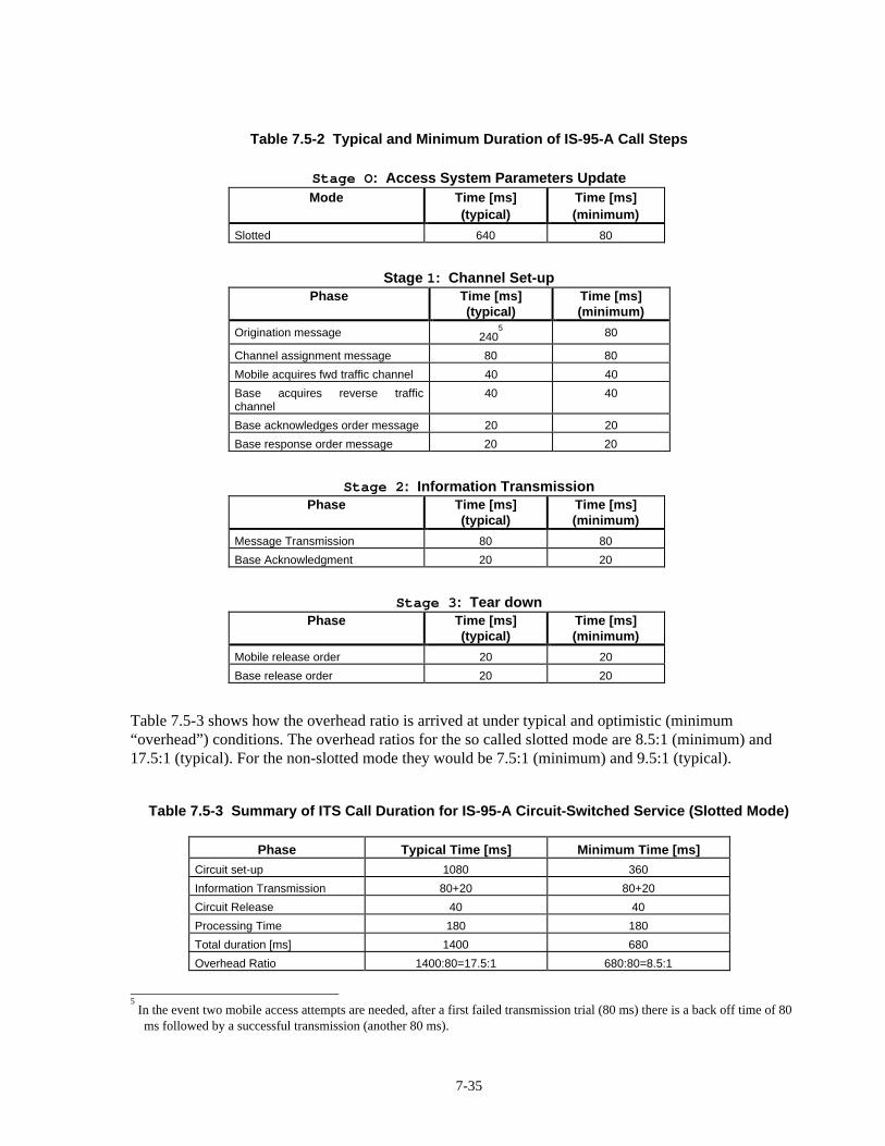
7-35
Table 7.5-2 Typical and Minimum Duration of IS-95-A Call Steps
Stage O : Access System Parameters UpdateMode Time [ms]
(typical)Time [ms](minimum)
Slotted 640 80
Stage 1: Channel Set-upPhase Time [ms]
(typical)Time [ms](minimum)
Origination message 2405 80
Channel assignment message 80 80
Mobile acquires fwd traffic channel 40 40
Base acquires reverse trafficchannel
40 40
Base acknowledges order message 20 20
Base response order message 20 20
Stage 2 : Information TransmissionPhase Time [ms]
(typical)Time [ms](minimum)
Message Transmission 80 80
Base Acknowledgment 20 20
Stage 3 : Tear downPhase Time [ms]
(typical)Time [ms](minimum)
Mobile release order 20 20
Base release order 20 20
Table 7.5-3 shows how the overhead ratio is arrived at under typical and optimistic (minimum“overhead”) conditions. The overhead ratios for the so called slotted mode are 8.5:1 (minimum) and17.5:1 (typical). For the non-slotted mode they would be 7.5:1 (minimum) and 9.5:1 (typical).
Table 7.5-3 Summary of ITS Call Duration for IS-95-A Circuit-Switched Service (Slotted Mode)
Phase Typical Time [ms] Minimum Time [ms]Circuit set-up 1080 360
Information Transmission 80+20 80+20
Circuit Release 40 40
Processing Time 180 180
Total duration [ms] 1400 680
Overhead Ratio 1400:80=17.5:1 680:80=8.5:1
5 In the event two mobile access attempts are needed, after a first failed transmission trial (80 ms) there is a back off time of 80
ms followed by a successful transmission (another 80 ms).

7-36
The column marked “Typical Time” in Table 7.5-3 provides:
• Circuit set-up time [ms]: Stage I (640) + Stage II (240+80+40+40+20+20) = 1080
• Transmissions of other than ITS payload bits [ms]: Stage III (20) + Stage IV (20+20) = 60
• Processing Time [ms] = 180; Total overhead (items 1 through 3) [ms] = 1320;ITS message transmission [ms] = 80
• Overhead ratio = (1320+80)/80 = 17.5
The numbers in the previous tables were arrived at in less than an optimistic analysis, which somewhatunderestimates the time needed to accomplish certain tasks. That approach therefore yields a totalduration figure which lower-bounds the real duration to be expected in the field. Two examples of thisoptimistic analysis are described below:
1. Ignored times — to allow a meaningful comparison with other ITS candidate technologies, theclock is started from the moment the user originates a message transfer. Thus, previous setuptimes, such as those taken for power up and first initialization, are ignored in the call durationbudget.
2. Shortened access time — it is assumed that two mobile access attempts (probes) are enough toget the base station response. Field and preliminary analysis suggests that this is typical, but farfrom worst case.
The comparison with a packet radio system, such as CDPD, does not favor circuit-switched CDMA data.Figure 7.5-7 shows the typical call durations (ignoring the effect of the ITS data load) with the delaycurves for CDPD which provides packet-switched service on a random-access protocol platform. ForCDPD, at S~0 Erlang, the overhead ratio is by definition 1:1 — given that the reverse link CDPDchannel is contention based, if there is no offered traffic, any message will go through without any delay(provided enough C/I is available). Consequently, it is apparent from the figure that the use of CDPD asthe platform for ITS will result in equivalent “overhead ratios” varying from 1:1 (at S~0 Erlang) to 9:1(at S~0.7 Erlang). This is always less than even non-slotted CDMA. It can be seen that even under themost optimistic assumptions, IS-99 remains a grossly inefficient platform for the purpose of carrying theusually small ITS messages.

7-37
10
100
1000D
ela
y [m
s]
0 0.1 0.2 0.3 0.4 0.5 0.6
CDPD
CDMA: Slotted mode/typical
CDMA: Slotted mode/min
CDMA: Non-Slotted mode/typical
CDMA: Non-Slotted mode/min
Lines represent lower bounds on CDMA delay(no dependence on throughput is assumed)
S-Throughput [Erlang]
Figure 7.5-7 Average Delay/Call Duration Ratio: CDPD versus Circuit-Switched CDMA
7.5.1.1.2.2.2 CDMA Short Message Service (IS-637)
IS-95-A based CDMA currently has very limited packet-switched data capabilities. The primarylimitation is imposed by the reverse link. On the forward link, the paging channel can be used toaccommodate outbound traffic, although the maximum data rate is currently restricted to 9.6 kbps underIS-95-A, or 14.4 kbps under TSB-137. On the reverse link, two mechanisms exist which can be used tofacilitate data traffic.
The existing IS-95-A channel structure associates a group of reverse access channels with a singleforward paging channel. The paging channel is used to carry system configuration information as well asuser data. Up to seven paging channels can be supported currently, each delineated within a cell sector bya separate Walsh code. Different sectors within the network are delineated by covering all channels in thesector with a complex valued pilot code. The modulation employed on the paging channel is essentiallyBPSK, using data rates of either 4.8 kbps or 9.6 kbps. Currently, there are 64 Walsh codes forchannelization on the forward link. Extensions permitting each Walsh code to be reused to facilitategreater capacity and/or data rates have been proposed. The paging channel is currently segmented intofixed 80 ms slots.
Associated with each paging channel are 32 reverse link access channels. Access channels are chosen atrandom by users and are delineated by non-orthogonal codes. The codes within a sector are a function ofthe sector pilot code, paging channel code and the access channel chosen. The random access protocolemployed is based on slotted ALOHA, with the slot size being a system configurable parameter. Theparameters governing the protocol permit additional randomization of packets through time offsets tofurther reduce the possibility of collisions. All packets employ a minimum of 20 ms (one frame) of un-modulated preamble to allow for acquisition by the base station. The access channel data rate is currentlyfixed at 4.8 kbps, with 64-ary orthogonal modulation being employed.

7-38
For long messages, as we have discussed, negotiation of a dedicated traffic channel is warranted. Whilethe traffic channel is capable of supporting 9600 bps sustained, the set-up times can be prohibitively longfor short messages (~800 ms), as reviewed in the previous section.
Short messages of 110 bytes or less can be accommodated by using the one-way data burst message onthe access channel. The peak data rate supported by the access channel is, as mentioned above, 4.8 kbps.
7.5.1.1.2.2.3 Packet-Switched Data (IS-657)
A new packet-switched data standard over CDMA (IS-95-A and TSB 174) has already been submitted toballot. Service Option 7 provides generic PPP support for packet data services. An accompanying ServiceOption 8, which would have supported CDPD networks was vetoed by Lucent Technologies (ex-AT&T)pending clarification of Intellectual Property Rights (IPR) associated with the CDPD standard, and TIA’srecognition of the CDPD standard. In any case, the support of PPP allows for interaction between the twonetworks.
The main limitation of this packet data service is its data rate, limited to 9.6 kbps for IS-95-A or 14.4kbps for TSB 174, significantly less than the 19.2 kbps of CDPD.
7.5.1.1.2.2.4 High Speed Data Services over CDMA
The CDMA Development Group (CDG), an autonomous organization of CDMA manufacturers andfuture carriers, is already in the process of standardizing the future high speed data services, both circuit-switched and packet-switched, over CDMA. The goal is first to standardize the 64 kbps services, andthen define multimedia data services at 500 kbps, and eventualy at 1-2 Mbps. Unfortunately, any of thesenew data services will definitely require re-designing the CDMA physical layer, and thus imply still along process.
7.5.1.1.2.3 Omnipoint’s Hybrid CDMA/TDMA/FDMA System (IS-661)Omnipoint’s PCS proposal is now an official industry standard under the designation IS-661.Omnipoint’s system can be integrated into either the GSM or AIN switching networks. It also allows forthe use of IS-41 inter-operability for roaming and system interconnection. In addition, the handset canoperate with both (GSM and AIN) networks, which enables easy roaming and inter-operability. Thesystem also provides inter-operability with indoor, low-cost, privately owned systems that offer wirelinequality voice and high data rates, while providing for full vehicle mobility (up to 65 mph) and ubiquitouscoverage. A high level architecture for Omnipoint’s system is depicted in Figure 7.5-8.

7-39
Figure 7.5-8 Omnipoint’s System Architecture and Public-Private Operation
Omnipoint’s system attempts to combine the major advantages of CDMA, TDMA, and FDMA in ahybrid solution. All signals employ a proprietary spread spectrum modulation waveform. Within a cell,multiple access at the data level is achieved through time division (TDMA). Either time-divisionduplexing (TDD) or frequency-division duplexing (FDD) can be used. In a standard configuration thistechnology provides 9.6 kbps full-duplex service to 16 simultaneous users in a single 1.875 MHz channel(or 32 users in 3.75 MHz). The 9.6 kbps reflect user throughput after all overhead for addressing, errorchecking, etc.
Adjacent cells are set to different frequency channels (FDMA) under a nominal N=3 frequency reusearchitecture (like in GSM). Cells beyond those immediately adjacent use a variety of separationtechniques, including different PN codes (CDMA), power control, directional antennas, and Time SlotInterchange (TSI) for additional inter-cell isolation. By utilizing a TDMA approach within a cell, and notrelying solely on CDMA for separating multiple mobile signals at the base station, self-interference at thereceiver is greatly reduced, permitting greater area coverage for a given mobile transmitter power.
Unlike CDMA-only architectures, cell sizes remain constant as a cell becomes loaded near capacity.CDMA is used in the Omnipoint system to mitigate multipath while providing high data rates, and toachieve better C/I ratios for inter-cell isolation.
Omnipoint’s TDMA structure is based on a 20 ms polling loop for mobile access to the base station. Inthe 1.875 MHz per RF channel version, the system provides 32 simplex time slots, each of 9.6 kbps, or16 paired, 9.6 kbps full-duplex time slots per RF channel. In the 3.75 MHz version, a single RF channelsupports 64 simplex time slots or 32 full duplex users each at 9.6 kbps. There are provisions for eachmobile to aggregate multiple time slots, giving users more bandwidth for higher data rates as required, toa maximum data rate of 153.6 kbps (higher than the 144 kbps of ISDN) full duplex per 1.875 MHzchannel.
In fact, the Omnipoint system is reported to support data rates from Short Message Services to ISDN datarates and higher. In its 1.875 MHz version it can support over 144 kbps full duplex and over 256 kbpssimplex. In the 3.75 MHz version it can support over 256 kbps full duplex or 512 kbps simplex. Note,however, that these higher data rates can only be achieved if the time slots are not in use by someone

7-40
else, which is not what the system is designed for. Moreover, no data protocol has been defined orselected for this variable rate data service.
In addition to the user voice/data channel, the system provides for a D channel that allows for continuous400 bps data traffic for every user. This channel is separate from (but simultaneous with) the bearerchannel for messaging even when the handset is in use. The D channel can carry information forapplications such as paging, voice mail notification, and Short Message Service.
The Omnipoint system is frequency agile in the entire 1850-1990 MHz band, including the unlicensedband (1910-1930 MHz) recently allocated to PCS by the FCC. It can also make use of the unlicensedband at 2.4-2.483 GHz). This aspect enables the system to be simultaneously used as an outdoor mobile,with in-building PBX, key system, or Centrex, or as a residential cordless phone.
Omnipoint’s base stations are very small (as small as 27”x15”x13”), and light (less than 100 pounds),enabling them to be pole-mounted on street lights, or telephone/utility poles, or attached to the sides ofbuildings. The cell radius varies from 100 feet to 10 miles, depending on the environment (urban,suburban, rural) and the height of the antennas used.
Omnipoint was granted a Pioneer’s Preference 30 MHz PCS license to compete in the New York MajorTrading Area (MTA). The IS-661 system will apparently be launched on top of a GSM (PCS 1900)system Omnipoint will deploy soon.
7.5.1.1.2.4 PCS 1900 (GSM/DCS 1800)Another technology candidate that requires evaluation is GSM, the well established Pan-Europeancellular standard. Actually, the American version of its DCS 1800 incarnation, PCS 1900, is what isproposed for evaluation here. The recent PCS auction results make it essential to analyze the proposedGSM solution. Pacific Bell Mobile Services, Bell South Personal Communications, American PersonalCommunications (APC), Western Wireless Co., Intercel, American Portable Telecommunications, andOmnipoint recently formed the North American Interest Group of the GSM MoU, and are all adamant todeploy GSM as soon as possible. Together, this group holds licenses to cover over 125 million people,including 12 of the top 25 cities in the U.S. In fact, APC, teamed with the Sprint TelecommunicationsVenture (a partnership between Sprint and the nation’s largest cable companies), recently deployed thefirst commercial PCS systems in Washington, DC, Maryland, and Virginia, with a population base ofmore than eight million people.
In addition to voice, GSM offers certain data capabilities under the form of short message services(SMS). Besides SMS, the recent availability of circuit-switched data equipment will also be analyzed forits suitability to ITS services.
Within the scope of GSM Phase 2+, still in progress and under no disclosure at ETSI (EuropeanTelecommunications Standards Institute), a true packet data service is being designed for use with GSM,namely GPRS, General Packet Radio Service. Similarly, a High Speed Circuit Switched Data (HSCSD)standard is in the works. Both will be briefly discussed below.
7.5.1.1.2.4.1 GSM System Description
GSM (initially named after the standards body that conceived it, Groupe Speciale Mobile), now standingfor Global System for Mobile Communications, refers to the Pan-European standard for digital cellularmobile telephone service. This system is being deployed throughout Western Europe, replacing firstgeneration mobile systems conforming to five different incompatible standards, and has enjoyedconsiderable success in many countries (128 have already signed agreements to deploy GSM systems).
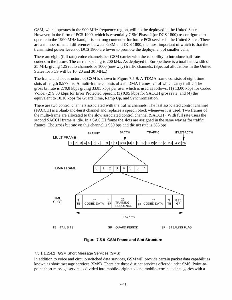
7-41
GSM, which operates in the 900 MHz frequency region, will not be deployed in the United States.However, in the form of PCS 1900, which is essentially GSM Phase 2 (or DCS 1800) re-configured tooperate in the 1900 MHz band, it is a strong contender for future PCS service in the United States. Thereare a number of small differences between GSM and DCS 1800, the most important of which is that thetransmitted power levels of DCS 1800 are lower to promote the deployment of smaller cells.
There are eight (full rate) voice channels per GSM carrier with the capability to introduce half-ratecodecs in the future. The carrier spacing is 200 kHz. As deployed in Europe there is a total bandwidth of25 MHz giving 125 radio channels or 1000 (one-way) traffic channels. (Spectral allocations in the UnitedStates for PCS will be 10, 20 and 30 MHz.)
The frame and slot structure of GSM is shown in Figure 7.5-9. A TDMA frame consists of eight timeslots of length 0.577 ms. A multi-frame consists of 26 TDMA frames, 24 of which carry traffic. Thegross bit rate is 270.8 kbps giving 33.85 kbps per user which is used as follows: (1) 13.00 kbps for CodecVoice; (2) 9.80 kbps for Error Protected Speech; (3) 0.95 kbps for SACCH gross rate; and (4) theequivalent to 10.10 kbps for Guard Time, Ramp Up, and Synchronization.
There are two control channels associated with the traffic channels. The fast associated control channel(FACCH) is a blank-and-burst channel and replaces a speech block whenever it is used. Two frames ofthe multi-frame are allocated to the slow associated control channel (SACCH). With full rate users thesecond SACCH frame is idle. In a SACCH frame the slots are assigned in the same way as for trafficframes. The gross bit rate on this channel is 950 bps and the net rate is 383 bps.
1 2 3 4 5 6 7 8 1011 1213 14 15 16 17 18 19 209 21 22 23 24 25 26
SACCH IDLE/SACCH
MULTIFRAMETRAFFIC TRAFFIC
0 1 2 3 4 5 6 7TDMA FRAME
TIMESLOT 3
TB 57CODED DATA
57CODED DATA
1SF
1SF
0.577 ms
26TRAININGSEQUENCE
3TB
8.25 GP
TB = TAIL BITS GP = GUARD PERIOD SF = STEALING FLAG
Figure 7.5-9 GSM Frame and Slot Structure
7.5.1.1.2.4.2 GSM Short Message Services (SMS)
In addition to voice and circuit-switched data services, GSM will provide certain packet data capabilitiesknown as short message services (SMS). There are three distinct services offered under SMS. Point-to-point short message service is divided into mobile-originated and mobile-terminated categories with a

7-42
service center being one of the endpoints in both cases. The two services can be combined to form amobile-to-mobile service via the service center. The messages in these services are limited to 160characters and are carried in control channels. The third category is cell broadcast SMS which allowsmessages to be broadcast on the control channel. Message length is limited to 93 characters. However,there is a provision to concatenate 15 such messages of 93 characters each. Unlike point-to-point SMS, amobile may not be able to receive a message broadcast on the control channel if it is in the middle of acall. However, this service has not been fully defined or implemented yet.
The point-to-point short messages services described above are carried in what is known as the slowaccess control channel (SACCH) which occupies one frame out of the 26 in the GSM multi-framestructure. The SACCH frame, like traffic frames, is composed of eight time slots. In a SACCH frame thetime slots are assigned in the same way as for traffic frames. That is, one is dedicated to each of the eightvoice channels. Thus, a digital message can be transferred efficiently if a voice call is in progress.However, use of the short message service in the absence of an existing voice call is rather inefficient,since the time slots normally used by the voice call would be unused.
7.5.1.1.2.4.3 Circuit-Switched Data
Unfortunately, only scant information is available. The manufacturers promote the equipment as adapters(no longer modems!) that allow the user to send faxes and data at up to 9.6 kbps over the GSM air-interface. The users can retrieve e-mail messages through a connection to their Internet service providerof choice, but do not have full IP capabilities -- the adapter does not have an IP address.
7.5.1.1.2.4.4 High Speed Circuit Switched Data (HSCSD)
A High Speed Circuit Switched Data (HSCSD) transmission mode is currently being standardized atETSI. HSCSD is a GSM bearer service intended to use multiple consecutive time-slots for increased datarate over the GSM air interface.
7.5.1.1.2.4.5 General Packet Radio Service (GPRS)
A new packet-switched data service over GSM, General Packet Radio Service (GPRS), is in the workingsat ETSI. The standardization process is still under way, and only preliminary, vague information isavailable. A comparative study of this new packet data system (and its associated network) with CDPDwould be quite instructive. Two things, however, seem certain. First, each data channel cannot providemore than 9.6 kbps, and to get higher throughput two or more TDMA time slots within a GSM carrierframe have to be used. A similar concept is proposed in CDPDng, except that each CDPD channel hasnow 19.2 kbps, and each CDPDng channel will have 56/64 kbps.
7.5.1.1.2.5 Private Mobile Data NetworksA few data systems exist in the land-mobile radio (LMR) 800-900 MHz band (in fact, part of this band isSMR), mostly of a proprietary nature. To the extent possible, these proprietary systems will be analyzedbriefly, with emphasis on capacity, availability, and coverage. The most important ones, in terms ofcoverage, are ARDIS and RAM. (RAM effectively operates in the SMR band.)

7-43
7.5.1.1.2.5.1 ARDIS
ARDIS (Advanced Radio Data Information System) is a two-way packet radio service. It was launched in1983 as a joint venture between IBM and Motorola, and is now a wholly-owned subsidiary of Motorola.ARDIS is deployed in 400 metropolitan areas (see example of coverage in Figure 7.5-10), reaching over90% of the urban business population, and 80% of the total U.S. population including Alaska, Hawaii,Puerto Rico, and the U.S. Virgin Islands. ARDIS has 45,000 users in the US, and another 7,500 inCanada, serviced by Bell-ARDIS, a subsidiary of Bell Mobility Canada. IBM is still ARDIS’ largestcustomer, with more than 12,000 field engineers using the service.

7-44
Figure 7.5-10 ARDIS Coverage in the Mid-Atlantic and Southern California Regions

7-45
The ARDIS network (Figure 7.5-11) consists of four network control centers with 32 network controllerspresiding over 1250 base stations. Remote users access the system from laptop radio terminals thatcommunicate with the base stations. The backbone of the network is implemented with leased lines. Thefour ARDIS hosts (Chicago, New York, Los Angeles, and Lexington, KT) serve as access points for acustomer’s mainframe computer, which can be linked to an ARDIS host via async, bisync, SNA or X.25dedicated circuits.
Four Network Control Centers
BS BS BS BS BS BS BS BS BS
Network Controler1
Network Controler2
Network Controler32
... ... ...... ......
...additional controlers can be installed
Figure 7.5-11 ARDIS Network Architecture
The system architecture is cell-based, with cells overlapped to increase the probability that the signaltransmission from a portable will reach at least on base station. The base station power is 40 W, and thecell radius extends to 10-15 miles. Portables operate with 4 W radiated power. The overlapping coverage,combined with error-correcting coding ensures that ARDIS can support portable communication frominside buildings, as well as on the street.
ARDIS uses a concept known as single frequency reuse, where all cells in a given area share a singlefrequency. While the use of overlapping coverage, and the same frequency, does provide for reliableradio connectivity, it raises the problem of interference when signals are transmitted simultaneously fromadjacent base stations. To deal with this, ARDIS turns off neighboring transmitters for 0.5 to 1 secondwhen a forward link transmission occurs. The system uses very little spectrum, but single frequencyreuse significantly limits system capacity.
ARDIS operates in the 806-821 MHz (reverse link) and 851-866 MHz (forward link) bands, and thechannel bandwidth is 25 kHz. The multiple access method is FDMA.
ARDIS has recently implemented nation-wide roaming and is in the process of raising the data rate in afew markets to 19.2 kbps (8 kbps of user information) from 4.8 kbps. Initially, ARDIS offered MDI’s(Mobile Data International Inc.) proprietary MDC-4800 protocol that achieved only 4.8 kbps on the 25kHz channel using FSK modulation. Recently, Motorola developed and began offering its proprietaryRD-LAP protocol for ARDIS, offering 19.2 kbps on the same channel using QFSK – with significantlyless overhead, nationwide roaming, more robust link layer protocols and coding schemes, and betteroverall message throughput. Today, the ARDIS network accepts both protocols and offers modems thatcan be configured for either of them.
The laptop terminals access the network using digital-sense multiple access (DSMA). Essentially, aremote terminal listens to the base station transmitter to determine if a “busy bit” is on or off. When it isoff, the terminal is allowed to transmit (very much like in CDPD). However, if two remotes begin to

7-46
transmit at the same time, the packets may collide, and re-transmission will be attempted. Unlike CDPD,however, the system does not have Collision Detection. Therefore, the system has to reject the garbledpackets and it will take a certain time for the remote terminals to realize that such an event took place.The busy bit only lets a remote terminal know when other terminals are transmitting, thus reducing theprobability of packet collision, but does not allow the system to “immediately” react to collisions.
As a packet switched data network, ARDIS carries only data, and does not offer any voice integratedproducts. The packet length is 256 bytes. The service is suitable for transmission of files up to 10 kbyteslong. ARDIS is used in support of computer-aided dispatching, such as is used by field service personnel,often when they are at a customer’s premises.
7.5.1.1.2.5.2 RAM
RAM Mobile Data, a joint venture of Bell South and RAM Broadcasting Corporation, introduced theMobitex system in 1991 in the U.S. Today, the network covers almost 100 metropolitan areas, and hasaround 30,000 users in the U.S., with another 2500 in Canada serviced by Cantel Data (Rogers Cantel).RAM plans to cover most of the U.S. business population, and is targeting the mobile professional.
The Mobitex system is a nationwide, interconnected trunked-radio network developed by Ericsson andSwedish Telecom. The first network that went into operation was in Sweden in 1986; other networkshave been implemented in the meantime in a growing number of countries including Norway, Finland,Canada, UK, France, Germany, Netherlands, Belgium, Poland, Australia, Korea, Singapore, Chile,Nigeria, and recently Mexico. The Mobitex system specification is managed by the Mobitex OperatorsAssociation (MOA).
While the system was designed to carry both voice and data, the U.S. and Canadian networks are used toprovide data only.
The Mobitex network architecture is hierarchical, as shown in Figure 7.5-12. At the top is the NetworkControl Center, from which the entire network is managed. The top level of switching is the nationalswitch (MHX1) that routes traffic among service regions. The next level comprises regional switches(MHX2), and below that are local switches (MOX), each of which handles traffic within a given servicearea. Many reliability features are implemented, such as alternate network pathways, autonomousoperation at each network level, multiple connections between nodes, and a backup network controlcenter.

7-47
BASBASBASBASBASBAS
Network Control Center
Multichannel Base Stations
Local Switches
Regional Switches
National SwitchesMHX1 MHX1
MHX2 MHX2 MHX2 MHX2 MHX2 MHX2
MOX MOX MOX MOX MOX MOX
Figure 7.5-12 MOBITEX Network Architecture
Mobitex uses packet-switching techniques to allow multiple users to share channels. Message packets areswitched at the lowest possible network level (only billing information is sent up to the network controlchannel).
The Mobitex system operates in much the same way as a cellular telephone system, except that hand-offsare not managed by the network. When a radio connection is to be changed from one base station toanother, the decision is made by the mobile terminal, not by the network intelligence. To access thenetwork, a mobile terminal finds the base station with the strongest signal and then registers with thatbase station. When the mobile terminal enters an adjacent service area, it automatically re-registers withthe new base station, and the user’s whereabouts are relayed to the higher-level network nodes, providingfor the roaming capability. Other features include broadcast and store-and-forward messaging.
RAM operates in the SMR band (896-901 MHz for the reverse link; 935-940 MHz for the forward link),in 12.5 kHz channels. The system’s transmission rate is 8 kbps half duplex, and the modulation isGMSK. Block interleaving, forward-error correction (FEC), as well as selective ARQ, are used to ensurethe integrity of the delivered data packets. A reservation slotted-ALOHA-type scheme is used for channelaccess, providing a good balance between efficiency and responsiveness.
RAM supports existing standards such as X.25 and TCP/IP through gateways, since it is based uponproprietary protocols. Mobitex uses a proprietary network layer protocol (MPAK) with up to 512 bytesof user data per packet, and 24 bit addressing (Mobitex Access Number). A transport protocol, MTP/1,also proprietary and optimized for the mobile radio environment, was introduced by the MOA tofacilitate development of multi-packet applications. The standard, proprietary Mobitex terminal interface,MASC (for Mobitex ASyncronous Communication), provides for reliable transfer of data to/from, andthe control and status monitoring of the modem.

7-48
7.5.1.1.2.6 ESMRSpecialized Mobile Radio (SMR), began as an analog system which is still used today mainly fordispatching of buses and taxis. Most SMR providers cover only a relatively small area, though many dooffer some sort of networking and interconnection with the public telephone network. Roaming underSMR is less user friendly than under cellular, and though it is technically possible to send data overSMR, it is not practical; SMR mainly offers wide-area analog voice dispatch service.
Enhanced SMR (ESMR) uses digital technology to allow more users per channel and to increase thenumber of services available to a user. ESMR providers such as Nextel, Dial Page, and CenCall ownlicenses to SMR frequencies across the country.
Some of the services provided by ESMR are dispatching, cellular-like mobile phone service,alphanumeric paging and messaging, and eventually other data services. An (E)SMR cell is larger than acellular telephone cell, meaning that it will be cheaper to cover a particular area, but the availablecapacity will be smaller. A disadvantage of ESMR is that the handsets are more expensive and bulkierthan current cellular phones, because of the new technology involved and the integration of voice anddata into one unit.
As with the mostly proprietary systems above, to the extent possible, the ESMR systems will be brieflyanalyzed, with emphasis on capacity, availability, and coverage. The main data entry is, at the moment,Geotek’s, since Nextel has not yet clarified its data options.
7.5.1.1.2.6.1 Nextel
Nextel Communications Inc., after completing the acquisition of Dial Call Communications Inc.,OneComm Corp., and American Mobile Systems Inc., as well as Motorola’s SMR licences, and aftergetting Geotek’s network (in exchange for 900 MHz spectrum), owns FCC licenses to a potentialcustomer base of 180 million people. Nextel, the only nationwide SMR provider, already has 916,000subscribers (approximately 80% of the total). Their plan is to build a nationwide digital network tocompete with cellular voice. No plans to provide packet data service have been announced yet, but theyhave circuit switched data and fax capabilities.
7.5.1.1.2.6.2 Geotek
Geotek uses a proprietary Frequency-Hopping Spread Spectrum system to provide circuit-switched voiceand data, as well as packet data services. The packet data service is TCP/IP based, and an option toprovide CDPD compatibility is in preparation. Geotek’s macro cellular system supports hand-off, andprovides 9.6 kbps raw data rate.
Services offered are cellular-type voice, half-duplex dispatch, full-duplex private telephony, two-waymessaging, and data dispatch. Geotek has already deployed its system in Philadelphia, New York,Baltimore, Washington, DC, and Boston, and is now deploying in Miami.
The network can provide information to mobile users through the Geotek Mobile Workstation and a top-of-the-line device that combines the functions of a cellular phone, two-way radio, pager, and PDA, orthrough a simple add-on to a cellular phone.
7.5.1.1.2.7 220 MHzThe 220 MHz service is a land mobile radio service that may be used for either commercial or privatepurposes. The service consists of two hundred 5 kHz paired channels, some of which are licensed on anational basis and some on a "local" basis. One hundred of the two hundred channel pairs are licensed as

7-49
five-channel trunked systems on a local basis. There are few restrictions as to the type of service that maybe provided by these systems. Some view this service as a potential competitor to PCS, cellular, or widearea SMRs, but the limited channel capacity will hinder its competitiveness unless license consolidationsoccur in the future.
7.5.1.1.2.8 Narrow-Band PCSTwo-way paging or messaging systems are among the first services that will utilize the Narrow-bandPersonal Communication Services (PCS) frequency band. The Federal Communication Commission(FCC) defines Narrow-band Personal Communication Services (PCS) as a family of mobile services thatincludes advanced voice paging, acknowledged paging, data messaging and both one and two-waymessaging on a nationwide, regional, major trading area, and basic trading area basis. The FCC haslicensed Narrow-band PCS at 901-902 MHz, 930-931 MHz, and 940-941 MHz. Six companies have paida total of $617 million for 10 nation-wide, narrow-band PCS licenses for channels in the 930 MHz band.The Narrow-band PCS providers include: AirTouch Comm. Inc., Bell South Wireless Inc., Destine Corp.(in fact MTel), McCaw Cellular (now AT&T Wireless), Pagenet, and Pagemart.
7.5.1.1.2.8.1 Two-Way Paging
SkyTel is presently offering the first two-way messaging service. This service uses Motorola’sReFLEXTM50 two-way transport protocol, and the TangoTM 2-way pager. SkyTel offers paging service inapproximately 300 markets; two-way paging is being deployed nationwide, and is offered now in the topmarkets.
Fundamentally, a two-way messaging service is similar to the existing paging services with an addition ofa response channel. Applications include: message reply, message initiation, and control actions such asautomatic registration and acknowledgment.
A two-way paging/messaging system is not an interactive system. The messages are stored, queued, andthen sent to the subscriber. Therefore, the system has an inherent delay that can be on the order of manyseconds to a few minutes. Such a system is clearly not suitable for supporting ITS messages that requirereal-time response. However, 2-way messaging may suffice for personal access type messages that don’trequire immediate response and are not time critical.
The candidate ITS messages that could utilize two-way paging are those with the following attributes:
• Short (up to 500 characters)
• Messages that can be responded to using a set of canned responses
• Messages that can tolerate long delays and do not require real time response
• Messages that are not time critical
Tables 7.5-4 and 7.5-5 provide the specifications of SkyTel’s paging/messaging service and Motorola’sTangoTM 2-way paging unit.

7-50
Table 7.5-4 SkyTel 2-Way Paging Service Specifications
Features SpecificationsMessage type Text and binary
Maximum Message size 500 character per transmissionBroadcast Rate (update) The message is transmitted once every 5 minutes for the 1st hour, and
once every hour for the next 72 hoursCoverage Over 100 markets -coverage will be similar to regular paging
Hardware Cost $400 for the Motorola TangoTM
Present Service Cost $40 to $90 per month (wide area, regional and nationwide)200 messages free (80 characters per message)$0.5 for each additional message
Capacity Similar to pagingInterface Methods to a
subscriberTelephone keypad, Operator, computer interface (i.e. modem),alphanumeric pager, Tango messaging unit, Electronic mail, andMessage Duet system
Subscriber RespondMethods
• Selecting a response from a set of pre-programmed responses• Selecting a response from a set of multiple choice options that are
included in the message• Using a palmtop to respond or initiate a message.
Table 7.5-5 Motorola’s Tango TM Two-Way Messaging Unit Specifications
Features SpecificationsFrequency Band Receiver 940-941 MHz (Narrowband PCS)
Transmitter 901-902 MHzChannel Spacing Receiver 25 kHz
Transmitter 12.5 kHzBit rate Receiver 6.4 kbps
Transmitter 9.6 kbpsSignaling Format QFSK
Received message type Numeric (4 bit data), alphanumeric (7 bit data), or binary data (8 bit). 8 bitsystems are used for transmission of long messages.
External interface Serial RS 232 interface for initiating messages and sending longmessages using a palmtop computer
Message Memory 100k bytesCanned Messages Up to 120 preprogrammed messages
7.5.1.1.3 Satellite Systems – A SurveyDuring the next few years, many companies are planning to launch hundreds of satellites designed toprovide wireless communications to mobile users virtually anywhere on the globe.
Proposed systems will offer voice and data, or data only. Most will also offer position determination. Thedifferent systems will determine the position of the user by various techniques, some more accurate thanothers. Even without a radio location service built into the system, the user terminal may be integratedwith a GPS engine. It is important to assess those proposed systems in what they can offer for ITS usersin remote or poorly-serviced areas.
This section first compares the advantages and disadvantages of satellite-based versus terrestrial-basedmobile radio networks. Then, the different orbits and the different communication subsystem types arecharacterized.
The many proposed satellite systems are briefly analyzed, focusing mainly on their data capabilities.Currently operating satellite systems are also analyzed, including those providing positioning, like GPSand GLONASS.
7-51
7.5.1.1.3.1 Terrestrial versus Satellite Mobile Radio NetworksTerrestrial-based networks offer obvious, distinct advantages over satellite-based systems. Theseadvantages stem from the much shorter distances between the mobile terminals and terrestrial basestations compared to distances in the order of 200 to 36,000 km, over which satellite mobile terminalsmust operate. Terrestrial base stations are easier and cheaper to plan, deploy, and integrate into thenetwork then satellites. In comparison, a satellite system lacks the flexibility for adding more and morechannels as a function of traffic increases.
The relative advantages that are likely to hold for terrestrial mobile networks include:
• Cheaper and smaller terminals and lower call charges
• Superior radio coverage in urban and in-building areas
• Minimal signal propagation delay
• Greater network capacity
However, satellite-based networks can exploit a few advantages, such as:
• Wide-area coverage
• Network flexibility
• Broadcast capability
Wide-area coverage enables satellite networks to offer services nationally to customers who operate inrural areas. This may be at the expense of greater call charges and more expensive radio equipment thanconventional terrestrial services. However, it is possible to offer a diverse range of services using theinherent flexibility of satellite systems. By increasing the mobile terminal’s usefulness, effectively onecan expect user charges to be lowered. This enables the satellite service to not only complement, but alsoto compete against terrestrial mobile radio networks in certain market segments.
This is the bet on which all the proposed satellite systems are based. Industry analysts, however, think themarket is not big enough to accommodate the proliferation of satellite offerings, and that in the end onlya few will survive.
In any case, customers will naturally seek the cheapest, most reliable mobile communication system thatmeets their requirements. In high density population areas, terrestrial networks offer unbeatableadvantages. Therefore, mobile satellite services can be expected to be complementary to terrestrial-basedservices, primarily in outlying areas.
7.5.1.1.3.2 Orbits: Acronyms and CharacteristicsThe most frequently chosen orbit for communication satellites has traditionally been the geostationaryearth orbit (GEO), a unique circular orbit in the equatorial plane at an altitude of 35,786 km.Geostationary satellites can cover large areas of the globe and allow fixed pointing ground stations.Three such satellites would, in principle, be enough to cover the whole earth. However, they require hightransmitter powers and large antenna apertures. They produce long communication delays, and requirehigh cost and high risk satellite launches. Moreover, they do not properly cover high latitude regions ofthe earth. In fact, one deficiency of the GEO satellites is the low elevation look-up angle at higherlatitudes, such as in Alaska and North Canada (and Northern Europe as well). These areas require linkmargins of 20-30 dB to overcome blockages. Also, most of the Arctic and Antarctic regions do not haveany coverage from GEO satellites.

7-52
Looking at the link budget for a satellite link, four terms can be identified:
1. Transmitter EIRP
2. Path Loss
3. Fade Margin + required C/No + Boltzman constant
4. Receiver G/T
In essence, the design of any satellite link involves consideration of the division of relative performancerequirements between the satellite repeater and the ground terminals. Given that path loss is practically aconstant (or is upper bounded) for a given orbit and frequency band, the important design parameters arethe G/T ratios and the EIRP values of the satellite and the earth terminals. These are determined by theantenna gains, receiver noise, and transmitter power, which then become the design variables.
Each communication satellite system design represents one solution to the cost/performance trade-off forthe system – taking into account the postulated population of terminals. The history of satellitecommunications began with small, low performance satellites and a few very large earth stations. Overthe years, satellites have grown in function and size. Earth terminals have decreased in size but increasedin numbers. These trends are due to the fact that the savings made on a large population of terminals canoffset the cost of satellite improvements.
The recent concept of Personal Communication Systems (PCS), however, requires a new approach to theequation. PCS terminals will be required to have small antennas, low output power, and high equivalentsystem noise temperature, i.e., they will be preferably hand-held terminals with very low EIRP and G/Tratio. Such a requirement presents a new challenge in system design.
There are three possible solutions to the problem of utilizing miniature terminals in satellitecommunications. The first is to further improve the performance of the satellite itself to compensate forsmall terminals. Some limitations exist to this approach, however. For instance, satellite receiver noiseperformance is limited by the noise temperature of the antenna looking at the “warm earth”. Moreoverthe satellite transmitter power is limited by the satellite power supply capability, a function of its mass. Ifa spot beam approach were used, increasing the satellite antenna gain (i.e., its size) would improve bothG/T and EIRP. However, the antenna size is restricted by the launch vehicle cargo capability, and by theantenna mass, complexity, and cost. In summary, increasing the satellite G/T and EIRP, with theassociated build-up in satellite mass and cost, may not be the most cost effective solution for the PCSdesign.
A second solution would be to use a frequency band at which even the small antennas would have highenough gains. For example, at the Ka-band (26-40 GHz), antenna gains of 20-25 dB can be achieved withsmall portable antennas. The use of such frequencies would also enable a GEO satellite cellular system toutilize a high number of cells with a satellite antenna array of moderate size and mass. The currentavailability of higher frequency bands mitigates in favor of this solution. However, several problemspresent serious impediments for such an approach. These include path loss increase with frequency, lowpower efficiency of Ka-band transmitters, dependence of link availability on weather, lack of technology,incompatibility with existing and projected terrestrial PCS systems (1900 MHz band).
A third, radically different solution is to decrease the path loss by bringing the satellite closer to earth, byplacing the satellites in lower orbits. In return for the advantages of lower path loss and shortercommunication delays, this technique unfortunately presents several disadvantages. Instead of the threesatellite geo-stationary constellation, many such non-geo-stationary satellites are required in order toprovide coverage equivalent to that of the geo-stationary system. The associated control telemetry andnetwork management systems become quite complex. In addition, high Doppler frequency shifts areintroduced into the satellite-terminal link, since the satellite is no longer fixed relative to the terminal.

7-53
Furthermore, inter-satellite cross links may be required for coverage extensions. Still, such a solution haspotential for reducing the cost of a satellite-based PCS system, and it is, as shown later, the preferredchoice within the proposed satellite systems.
The non-geostationary orbits are grouped as either low earth orbits (LEO), medium earth orbits (MEO),or highly elliptical orbits (HEO) as shown in Figure 7.5-13. LEO are those in the range 200-3000 kmbetween the so called constant atmospheric density altitude and the Van Allen radiation belts. MEO startabove 3,000 km, and extend up to GEO. Satellites in these orbits cross the radiation belts, and thus facehigh radiation levels.
Finally, HEO can put the satellite within several hundred kilometers of the earth’s surface, during itsinactive phase, and then take it even beyond the GEO, during its active phase. All elliptical orbits havetwo characteristic points: the perigee, point of closest approach to the earth, and the apogee, the pointfarthest from earth.
The choice of optimum satellite orbit is usually determined by the intended earth coverage. All stableorbits can be divided into four classes:
1. Inclined6 Circular geosynchronous7 orbits
2. Inclined Elliptical geosynchronous orbits
3. Non-synchronous orbits of the above two and the equatorial type
4. Geostationary8 orbits
Not all orbits are suitable for communications. Non-synchronous orbits are seldom used for commercialcommunications, although they may be preferred for defense and scientific applications. Class 1 circularLEO and MEO orbits are particularly suited for cellular mobile communications, since the cell sizesremain constant throughout the orbit. Constellations of geosynchronous satellites in polar and/or inclinedcircular orbits can be combined to provide optimum continuous earth coverage.
Most of the LEO and MEO orbits are polar. A MEO system however exists that borrows the name of itsorbit, ICO, Inclined Circular Orbit. This can cause some confusion, since an alternative, although lessaccurate acronym for MEO, more frequent in European literature, is Intermediate Circular Orbit (i.e.,ICO). Here, the most usual MEO acronym is used, reserving ICO for the proposed system with thatname.
A general problem with Class 2, low-perigee, inclined orbits is the rotation of the orbital plan due to theearth’s oblateness. This rotation would constantly move the coverage area. The larger the eccentricity,the smaller the perigee height, the shorter the period, and the greater the instability of the orbit. The onlyway to stabilize such an orbit is to use a particular value of inclination, namely 63.435°. One such stableinclined elliptical geosynchronous orbit is the so called Molnyia orbit. It has a period of half a sideralday, a perigee height of 500 km, and an apogee height of 39,800 km. The apogee of this orbit alwaysremains at a constant geographic latitude. Another orbit from this class with lower eccentricity is calledthe Tundra orbit. Its period is a full sideral day. In both cases, the most useful part of the orbit is theregion of the apogee (active phase); there the satellite appears to move slowly, and stays close to theobserver’s zenith for a long time.
6 Inclination is referred to the equatorial plane. Polar orbits are inclined 90°.
In a geo-synchronous orbit (classes 1 and 2), a satellite completes an integral number of orbits per day.
8 Geostationary orbits are geosynchronous orbits with a period of one day, the result is the relative stationarity of the satellite inreference to a point on the earth’s surface.

7-54
A final observation is that the higher the satellite orbit, the greater its coverage, the lower its relativevelocity and thus the Doppler shift, and the longer it stays above the horizon. The advantages arebalanced by the fact that the propagation delay worsens with increased satellite altitude.
MEO Satellites10,000-20,000 km height
HEO Satellitesin active phase
up to 42,000 km height
GEO Satellites~ 36,000 km height
Equatorial Plane
Inactive HEO phase
LEO Satellitesdown to 700 km height
Figure 7.5-13 Satellite Orbits
7.5.1.1.3.3 Communication Subsystem CharacterizationThe communication subsystem on a communications satellite consists of a number of repeaters whichamplify the signal received from the uplink, and condition them in preparation for transmission on thedownlink. Each repeater belongs to one of the following types:
• Transparent, Non-Regenerative, or Bent-Pipe Repeater, referred to as Transponder -- they performsolely a frequency conversion from the uplink band to the downlink band (the conversion may bedone in two or more steps);
• On-board Processing Repeater -- they first perform signal regeneration, and then they act as“switchboards in the sky”, circuit-switching between antennas, and possibly multiplexing thereconstructed received signal for transmission at a higher bit rate.
The advantage of the “transparent” repeater is that their transponders impose minimal constraints on thecharacteristics of the communication signals. For example, they are “transparent” to different modulationtypes, whether analog or digital. They therefore offer maximum flexibility for designers of largecommunication networks. However, there is the risk of increasing the bit error rate (BER) at eachconversion.
7.5.1.1.3.4 Proposed Satellite SystemsThe panoply of proposed satellite systems ranges from the ambitious, 840-satellite LEO constellationadvanced by Teledesic, to the “down-to-earth”, three-satellite GEO constellation of Skycell, includingalso the very vague, 12 satellites in the Ka-band for voice, data, and multimedia services proposal from

7-55
AT&T, an even more ambiguous 9-satellite proposal from Lockheed Martin for the same Ka-band, andthe Picosats concept, which calls for literally a myriad of pico-satellites which one can virtually own (ifone wishes to invest $50,000). The three latter systems are not analyzed herein for lack of concreteinformation.
Most of the mobile satellite systems are low earth orbit (LEO) systems, which are much closer to theearth than the geostationary (GEO) satellites normally used for telecommunications thereby significantlyreducing communications delay. Because of their proximity to earth, LEO systems accommodate low-powered and compact user terminals.
7.5.1.1.3.4.1 Little LEO’s
The little LEO’s are low earth orbit satellite systems that operate in the VHF range and carry only datacommunications. They are not very complicated, and are therefore easier and less expensive to build andoperate than a system that also carries voice communications, for example.
7.5.1.1.3.4.1.1 ORBCOMM
ORBCOMM plans a system of 20 LEO satellites costing less than $150 million. The ORBCOMM systemis a good example of a bent-pipe architecture, which all but two of the mobile satellite systems utilize.The mobile user sends a message to a satellite and that satellite routes the message to one of four gatewayearth stations located in the four corners of the continental United States.
The four earth stations will be connected to the network hub in Virginia and will route the message thereto determine where it should be sent. The messages can be sent from Virginia through the public andprivate e-mail networks, a leased line to a specific location, or back through the system to another mobileuser.9
ORBCOMM began operation in February 1, 1996 after successfully launching in April 1995 the first twosatellites of its intended 20/26/36 satellites constellation. (According to NASA, the two satellites hadcommunication problems after launching, but are now operational. Coverage of the two satellites isshown in Figure 7.5-14.) ORBCOMM has become the world’s first commercial satellite-based two-waymessaging and positioning system. However, from Error! Reference source not found., we can see thatthe first two satellites cannot offer more than sporadic coverage of the Continental U.S. This situationwill obviously improve with the deployment of further satellites.
9 It is not possible, in a bent-pipe architecture, to send a message from one satellite to another; the satellites basically link the user
with the land-based network.

7-56
Figure 7.5-14 Location of, and Coverage Provided by, the Two Already Deployed ORBCOMMSatellites at Two Instants in Time
ORBCOMM has signed up 17 candidates to become international users. They plan to charge about $1per message (100 byte), plus a fixed monthly fee. The terminal will eventually cost between $100 and$400 dollars.
7.5.1.1.3.4.1.2 STARSYS
Starsys is a U.S. company that provides global positioning services. It plans to start initial service in 1996with a data-only, two-way radio communications system with 24 satellites to connect remote users'portable terminals to a central ground station. Starsys claims it will be able to locate the terminal to

7-57
within 100 meters. The system is estimated to cost $200 million. Subscriber terminal costs are estimatedat $75 to $250 for the 3rd generation.
Like ORBCOMM, Starsys plans to offer emergency communication, stolen asset recovery, andhazardous materials tracking services.
7.5.1.1.3.4.1.3 Comparative Analysis
Issues that need clarification include multiple access technique, dual-mode versus single mode userterminals (cellular and satellite), supported mobility, and most importantly, overall system cost. Table7.5-6 provides the side-by-side comparison.
Table 7.5-6 Little LEO’s
SATELLITE SYSTEMS ORBCOMM STARSYS VITASAT
PARTNERSHIP Orbital Sciences Corp.,Teleglobe, TRW
North America Collection andLocation by Satellite(NACLS), and ST System
Volunteers In TechnicalAssistance (VITA,VITACOMM)
NUMBER OF SATELLITES 20, 26, 36 depending onreference
24 2 satellites since 1984, 3rdadded in 1995 (VITASAT-A,a.k.a. GEMSTAR-1)
COVERAGE US now, Global future Global Global, designed fordeveloping countriesincluding South America,Africa
SCHEDULED OPERATION Currently Operational in US;1996 Canada and Mexico;1997 Europe and LatinAmerica
1996 End of 1995
PERCENTAGE OFOBTAINED FINANCING
"100%" ? ?
FCC LICENSE late 1994 1992 Experimental License ?
DATA RATE (kbps) 2.4 uplink, 4.8 downlink ? ?
HAND-HELD vs. PORTABLEUSER TERMINALS
Portable and Hand-held ? Portable
USER TERMINAL COST $100 -$400 ? $3500
DATA RATE COST(US Dollars per kilobyte)
$1.00 per 100 bytes ? $50/month for up to 100kbytes
SERVICES two-way messaging, RDSS one-way data, two-waymessaging
two-way messaging; storeand forward with typically 90minute and as much as 12hour message delay.
TARGETED APPLICATIONS emergency comm. 2 way-mail, remote resourcemonitoring
emergency comm. stolenasset recovery, hazardousmaterial tracking
Store-and-forward data
7.5.1.1.3.4.2 Big LEO Systems
The big LEO systems are distinguished from the little LEO’s by their bandwidth. Big LEO’s operateabove 1 GHz and are able to carry voice as well as data. Most use more satellites for greater capacity andreliability. Because big LEO’s are able to carry voice, many of the systems will be marketed and pricedwith voice service in mind, meaning that sending data might not be as cost effective as it would be usinga little LEO system. Big LEO’s are also much more expensive to build and operate.

7-58
7.5.1.1.3.4.2.1 Constellation
Formerly called Aries, the Constellation satellite system consists of 48 satellites, and plans to provideservice for mobile phone users outside of cellular's coverage. Constellation Communications Inc. alsoexpects their service to be used in rural areas of developing nations, where installing telephone switchesand wires may not be cost-effective. The equatorial plane of the system, dubbed ECCO, will be deployedas a joint venture with Embratel, Brazil’s government telecommunications holding company.
7.5.1.1.3.4.2.2 GlobalStar
GlobalStar plans to commence initial commercial operation via a 24-satellite LEO constellation in 1998(full 48-satellites coverage is anticipated for 1999). The constellation will be deployed in a 1,410 kmorbit (resulting in no perceptible voice delay), and provides multiple satellite coverage (2-4 satellites willusually be visible at any time). The satellites are of the “bent pipe” type for simplicity and reliability, aswell as cost reasons. GlobalStar employs CDMA spread spectrum access techniques to provide fullglobal services.
GlobalStar intends to provide high quality telephony, data transmission, paging, fax, and positionlocation to areas currently poorly or not at all served by existing wireline and cellular systems. Theservice, however, has to be authorized by the local telecommunications regulatory authorities. Users ofGlobalStar should expect to make and receive calls using hand-held or vehicle-mounted terminals similarto today’s cellular telephones. Because the system will be fully integrated with existing fixed and cellularnetworks, GlobalStar’s dual-mode handset units will be able to switch from conventional cellulartelephony to satellite telephony as required. Calls will be routed to customers through existing public andprivate telephone companies. GlobalStar handsets will be able to be used as mobile phones anywhere inthe world using an individual subscriber number accessing either the local network or the satellitesdirectly.
The GlobalStar system consists of the same number of satellites as Constellation, though its expectedcapacity is much larger. The added complexity is reflected in the anticipated cost of $2 billion. $1.4billion has already been raised. Anticipated average call prices range from 35¢ to 53¢ per minutealthough this may seem optimistic. No data pricing information is available.
Leading an international coalition of companies teaming up to build the GlobalStar system are Loral andQualcomm and Space Systems/Loral. Their strategic partners are Air Touch Communications, Italy'sAlenia Spazio and Elsag Baley (Finmeccanica), France's Alcatel and France Telecom, Korea's DacomCorporation and the Hyundai Electronics Group, UK's Vodafone Group, and Germany's DASA (formerlyDeutsche Aerospace AG).
7.5.1.1.3.4.2.3 Iridium
Iridium plans to be operational in 1998 with a 66-satellite system for worldwide mobile communicationsservices to provide direct-via-satellite global voice, data, paging, and radio-determination services topocket terminals anywhere in the world. Total system cost is estimated at $3.4 billion.
Iridium will use TDMA whereas others plan to use CDMA. Five experimental models have approval for1996 to demonstrate system feasibility. The consortium includes Motorola, Sprint, Lockheed/Raytheon,Japan's Nippon Iridium, Saudi Arabia's Mawarid Corp., Canada's BCE Mobile, Venezuela's MuidiriInvestments, Italy's STET, Korea's Hyundai Electronics, Thailand's United Communications, Russia'sKrunichev Enterprises, China's China Great Wall Industry, Taiwan's Pacific Electric Wire & Cable Co.,India's Infrastructure Leasing & Finance Services, Germany's Deutsche Aerospace, and UK's VodafoneGroup.

7-59
Motorola's ambitious Iridium system incorporates inter-satellite links (see Figure 7.5-15), which greatlyraises the complexity of their satellites. A system with inter-satellite links, though, will be more robustand offer greater world-wide coverage than a comparable one without them. In an area without groundstations, a bent-pipe satellite would be unable to open a voice connection and could only store or sendpreviously stored messages to a mobile unit.
Figure 7.5-15 Iridium System Footprint at a Given Point in Time
7.5.1.1.3.4.2.4 Teledesic
By far the most ambitious LEO is Teledesic, an 840 “refrigerator-sized” satellites system backed by BillGates and Craig McCaw. The satellite trajectories to cover the globe are shown in Figure 7.5-16.Teledesic plans to operate in the 20/30 GHz range. Teledesic Corp. anticipates a basic channel rate of 16Kbps, and channels may be combined by fixed ground units up to a maximum of 50 Mbps. It also willincorporate inter-satellite links. Teledesic does not plan to be operational until 2001 and will cost at least$9 billion. Teledesic is not intended for mobile terminals.

7-60
Figure 7.5-16 Path Described by a Teledesic Satellite
7.5.1.1.3.4.2.5 Comparative Analysis
Key issues in the success of any of these systems will be voice and data service costs, user terminal costs,system security, and supported mobility. All this, however, assumes the systems get deployed, which isnot guaranteed given the huge costs involved. Obtaining the operating licences needed to provide serviceglobally is certainly not an easy task and is another area of risk. Table 7.5-7 provides a comparativesummary for the LEO satellite systems.

7-61
Table 7.5-7 Comparative Analysis of Big LEO’s
SATELLITE SYSTEMS CONSTELLATION(formerly ARIES)
GLOBALSTAR IRIDIUM TELEDESIC
LEADERSHIP ConstellationCommunication
Loral, Qualcomm Motorola Bill Gates ofMicrosoft, andCraig McCawfounder of McCawCellularCommunications,Inc. and chairmanof Teledesic
NUMBER OF SATELLITES 48 48 plus 8 spare 66 plus 6 spare 840 plus up to 84spare
COVERAGE Global within +/- 70degrees latitude
Global Global, except for2 degree hole atpoles; 95% ofearth's surface
SCHEDULED OPERATION 1998 1998 1998 2001PERCENTAGE OF OBTAINEDFINANCING
~15% ~70% ~100% ?
FCC LICENSE ? Jan. 1995 ? ?MULTIPLE ACCESSTECHNIQUE
CDMA CDMA FDMA/TDMA/TDD TDMA, SDMA,FDMA, AdvancedTDMA
VOICE CIRCUITS PERSATELLITE
? 2000-3000 1100 (power limited) 100,000 (16 kbpschannels)
VOICE RATE (kbps) 4.8 adaptive2.4/4.8/9.6
2.4/4.8 16
DATA RATE (kbps) 2.4 7.2 sustainedthroughput
2.4 16 to 2048
MOBILITY ? ? ? FixedDUAL-MODE vs. SINGLE MODEUSER TERMINALS (land andsatellite)
? DUAL DUAL SINGLE
HAND-HELD vs. PORTABLEUSER TERMINALS
Hand-held Hand-held Hand-held Portable
SYSTEM SECURITY ? ? ? encryptionSYSTEM COST(Million U S Dollars)
$1,700 $2,000 $3,700 $9,000
USER TERMINAL COST ? ~$750/terminal;$1000-$1200 fortelephone
$2500-$3000 ?
VOICE SERVICE COST(US Dollars per minute)
? $0.35-$0.55 $3.00 ?
DATA SERVICE COST(US Dollars per kilobyte)
? ? ? ?
SERVICES voice, data, fax Voice, data, fax,paging, shortmessage service,RDSS
Voice, data, fax, paging,messaging, RDSS
Voice, data, fax,paging, video
TARGETED APPLICATIONS extension of the cellularnetwork
worldwidecommunication
worldwidecommunication
ISDN to ruralbusinesses andremote terminals(fixed)
Note: The information in this table is based on inputs provided by the marketing organizations for the vendors andhave not been validated by the Architecture team.

7-62
7.5.1.1.3.4.3 Other Mobile Satellite Systems
A few companies believe LEO is not the best configuration for a mobile satellite system. Hence, they areproposing highly elliptical orbit (HEO), Medium Earth Orbit (MEO), and Geostationary (GEO) systems.
7.5.1.1.3.4.3.1 Ellipso
Ellipso plans to be operational in 1997 and to provide combined position determination and mobile voiceservices using up to 24 satellites. Six experimental spacecraft have approval from the FCC. They will useFDMA and CDMA techniques.
Ellipso's unique elliptical orbit will provide more coverage to areas with high traffic at a certain times ofthe day. For example, if the time of maximum duration visibility over New York were selected to be mid-day, maximum duration visibility for Chicago, Denver, and Los Angeles would also be mid-day. Tocomplement the elliptlical orbit, the Ellipso system has a second component, MEO, providing additionalcoverage of intermediate latitudes.
Ellipso also plans to become an extension to the cellular network, providing service where cellular is notavailable. Costs to users will be comparable to those of cellular. Contracts exist with countries includingCanada, Mexico, Israel, and Australia.
7.5.1.1.3.4.3.2 Odyssey
Odyssey is a MEO system. Its higher orbits allow it to cover the globe with only 12 satellites. Thesmaller number of satellites makes Odyssey slightly cheaper than the big LEO’s, but its capacity will besmaller, and user terminals will probably be more complicated and more expensive. Ground controlstations will serve as gateways to local networks for voice and data communications to hand-heldterminals worldwide.
Odyssey’s main partners are Teleglobe and TRW. Participants in the system design group include HarrisCorporation, France's Thomson-CSF, Canada's Aerospace Ltd. and Northern Telecom, Germany's ANTNachrichtentechnik GBH.
7.5.1.1.3.4.3.3 ICO Global Communications
ICO Global communications, backed by 44 international investors, plans to have its 10-satellite MEO (orICO), 10,400 km orbit system (see Figure 7.5-17) in service by the year 2000. When fully operational,the ICO system intends to provide a low-cost global satellite phone service, as well as data, fax, andpaging, using hand-held pocket-sized terminals. It will be fully complementary with terrestrialcellular/PCS. ICO is already a member of the GSM MoU, but it will also support D-AMPS and other 2ndand 3rd generation digital cellular systems.
Two or more satellites will be usually visible to the users at relatively high angles of elevation tominimize blocking by terrain, buildings, and other obstacles. The satellites will relay calls between theuser and a Satellite Access Node (SAN) within the satellite’s view. SAN’s are interconnected usingterrestrial facilities to form a network, the ICO-Net, and are linked through gateways to the PSTN.
ICO began as Inmarsat P, or Project 21, later spinning into a separate commercial entity, since its scopeexpanded beyond coastal areas. The system cost is estimated at $2.6 billion and $1.5 billion have alreadybeen secured. Hughes is ICO’s first strategic partner, and has invested an amount ($94 million)equal toICO’s largest non-institutional investors (Inmarsat invested $150 million, becoming the major investor).

7-63
Figure 7.5-17 ICO’s Satellite Orbits
7.5.1.1.3.4.3.4 Skycell
The American Mobile Satellite Corp. (AMSC) plans to offer voice, data, and location service with itsnew Skycell system, a series of three GEO satellites. Figure 7.5-18 shows the planned coverage. Becauseof the much greater distance to the satellites compared to LEO, hand held terminals will not be offered.Vehicle mounted units are expected. Skycell has already obtained an FCC license.

7-64
Figure 7.5-18 SKYCELL Coverage
7.5.1.1.3.4.3.5 MSAT
TMI and AMSC were the companies that initiated, funded, developed and launched the satellite that willbe used to provide commercial mobile satellite service in North America. Commercial service isanticipated for early 1996. MSAT extends mobile and fixed telephone (6.4 kbps codec), fax, data (2.4and 4.8 kbps), and dispatch radio communications to all of North America plus up to 400 km of coastalwaters, the Caribbean, and Hawaii, as well as Mexico and Central America. The system is fullyconnected to the PSTN, and to public and private data networks.
Figure 7.5-19 shows the type of terminal supported. Mobile units use a small 7” dome antenna, andtransportable units use a 30” flat antenna that can be easily set-up by the user. Call rates vary from $1.55to $2.75 per minute, depending on the plan, and on the service modality, fixed or mobile.

7-65
Figure 7.5-19 MSAT North American Coverage
7.5.1.1.3.4.3.6 Comparative Analysis
Issues of mobility, service, and terminal cost will be determinant for the success of MEO/HEO systems.Tables 7.5-8 and 7.5-9 provide comparison summaries for the MEO/HEO and GEO satellite systemsrespectively.

7-66
Table 7.5-8 Comparative Analysis of MEO and HEO Satellite Systems
SATELLITE SYSTEMS ELLIPSO ICO (formerlyInmarsat-P)
ODYSSEY
PARTNERSHIP Ellipso Inmarsat, MultipleGovernment Agencies,and Hughes
Teleglobe, TRW
ORBIT CLASS MEO and HEO MEO (IntermediateCircular Orbits, ICO)
MEO
NUMBER OF SATELLITES MEO is 6; HEO is 10 10 plus 3 spare 12 plus 3 spareCOVERAGE North of 50° South Global major land massesSCHEDULED OPERATION 1998 2000 2000SYSTEM COST(Million US Dollars)
$750 $2,600 $1,800
PERCENTAGE OF OBTAINEDFINANCING
? 59% ?
FCC LICENSE ? Aparently available ?MULTIPLE ACCESSTECHNIQUE
CDMA TDMA CDMA
VOICE CIRCUITS PERSATELLITE
? 4500 2300
VOICE RATE (kbps) 4.15 4.8 4.8DATA RATE (kbps) 0.3 to 9.6 2.4 9.6MOBILITY ? ? ?DUAL-MODE vs. SINGLE MODEUSER TERMINALS (land andsatellite)
Dual Dual Dual
DUAL-MODE vs. SINGLE MODEUSER TERMINALS (land andsatellite)
DUAL DUAL DUAL
HAND-HELD vs. PORTABLEUSER TERMINALS
Hand-held Hand-held Hand-held
USER TERMINAL COST ~$1000 or $300 add-onto digital cellular unit
"Several Hundred" ~$300
VOICE SERVICE COST(US Dollars per minute)
$0.50 $1-$2 $0.7 5 ; $24 monthlycharge
DATA SERVICE COST(US Dollars per kilobyte)
? ? ?
SERVICES Voice, data, fax, paging,messaging, RDSS
Voice, data, fax, paging Voice, data, fax, paging,messaging, RDSS
TARGETED APPLICATIONS extension of cellularnetwork
global phone integratedwith cellular services
extension of cellularnetwork
Note: The information in this table is based on inputs provided by the marketing organizations for the vendors andhave not been validated by the Architecture team.

7-67
Table 7.5-9 Comparative Analysis of GEO Satellite Systems
SATELLITE SYSTEMS INMARSAT (A,B,C,M) MSAT SKYCELLPARTNERSHIP Multiple Government Agencies
(International Maritime SatelliteOrganization, consortium of 76countries)
Mobile Satellite Corp.,Glentel, Inc., BCE, SparAerospace, Hughes,Mitsubishi, Westinghouse
American Mobile SatelliteCorp. (Hughes, AT&T, MTel,Singapore Telecom)
NUMBER OF SATELLITES Inmarsat phase 2: 4 satellites (since 1992);Inmarsat phase 3: 5 satellites (projected for 1996)
2 ?
COVERAGE Global North America, Hawaii,Caribbean
North America
SCHEDULED OPERATION Operational since 1993 1996 ?SYSTEM COST(Million US Dollars)
? ? ?
PERCENTAGE OF OBTAINEDFINANCING
? ? ?
FCC LICENSE WARC, WRC ? 1989MULTIPLE ACCESSTECHNIQUE
? TDMA/TDD FDMA
VOICE RATE (kbps) 6.4 to 16 depending on system ? ?DATA RATE (kbps) 0.6, 2.4, 9.6, 64 depending on
system2.4 1.2-4.8
MOBILITY Fixed to Aeronautical
Fixed (Canada and Alaska);Mobile (Contiguous 48States)
Full mobility (vehicles, ships,and airplanes)
DUAL-MODE vs. SINGLE MODEUSER TERMINALS (land andsatellite)
Dual (drivers for ARDIS, CDPD,GSM)
Dual ?
HAND-HELD vs. PORTABLEUSER TERMINALS
Portable Portable Portable
USER TERMINAL COST $5000-$35,000 depending onsystem
$5000-$6000 ?
VOICESERVICE COST(US Dollars per minute)
$2.00-$8.00 depending on system $2.50 Standard: $25/month, $1.49/minute
Business:$175/month, 200minutes free, $0.85/minutevoice, data, fax
DATA RATE COST(US Dollars per kilobyte)
$1.00-$1.50 ? similar to voice service costs
SERVICES Voice, data, fax, e-mail, store-and-forward, alerting, positiondetermination
Voice, data, fax, dispatchradio
Voice, data, fax, locationdetermination
TARGETED APPLICATIONS Worldwide communications Mobile office, positiondetermination, e-mail,monitoring, voice dispatching(2-way), broadcast andmulticast messaging
Transportation, maritime,aeronautical, remote siteindustries
Note: The information in this table is based on inputs provided by the marketing organizations for the vendors andhave not been validated by the Architecture team.

7-68
7.5.1.1.3.5 Operating Mobile Satellite Systems of Interest
7.5.1.1.3.5.1 OmniTRACS
In the late 80’s, QUALCOMM developed a geostationary (GEO) two-way Ku-band (11 and 13 GHz)data/messaging service called OmniTRACS. The system is spread-spectrum based, and is aimed atproviding position reporting and messaging services for the trucking community. By early 1992QUALCOMM had over 25,000 in use on trucks across North America and were successfully marketingtheir services world-wide. Today OmniTRACS claims more than 135,000 terminals all over the world,including its European counterpart, EutelTRACS, a joint venture of QUALCOMM and AlcatelQUALCOMM (established in 1990, 34% owned by QUALCOMM). Systems are currently operational inMexico, Brazil (where it is known as OmniSAT), Japan, Russia, and Malaysia.
The OmniTRACS system is a low-rate interactive data communication tool that links fleet dispatchcenters to their vehicles. This system uses QUALCOMM dedicated satellite systems, as well ascommercially available satellite systems (i.e., transponders) as needed, for providing the interactive dataservices. For example, QUALCOMM has signed an agreement with ORBCOMM giving it the right toresell ORBCOMM’s communication services with the OmniTRACS expanded trailer tracking and cargomonitoring applications.
The messaging and positioning information is sent, via satellite links, through the OmniTRACS NetworkManagement Center to the fleet dispatch center. The mobile communication units provide the computingcapability to send and receive text messages to and from the vehicles. The mobile units are also availablewith QUALCOMM’s Automatic Satellite Position Reporting (QASPR). QASPR uses satellitetriangulation to provide vehicle position to within 1/4 of a mile. The system also supports direct inputfrom Global Positioning System (GPS) receivers. The system uses a proprietary Ku-band directionalantenna that is encased in an aerodynamic dome. An electronically driven motor directs the antennatoward the satellite at all times. A new C-band system has been introduced for those regions where Ku-band is not readily available (e.g., Malaysia). In this case, vehicle tracking is made possible only throughthe use of a GPS receiver.
The OmniTRACS mobile terminal can be used for monitoring vehicle’s status. The sensor information ismade available to the driver using the onboard terminal, and is transmitted to the dispatchers. Because ofthe cost of the satellite terminal, this system is only suitable for long-haul truck operations that need verywide area coverage that includes remote areas.
7.5.1.1.3.5.2 INMARSAT Satellite Systems
Inmarsat (International Maritime Satellite Organization) was formed by a consortium of 28 foundingcountries upon adoption of the Inmarsat Convention in September 1976. The corresponding operatingagreement came into force in July, 1979. Today 76 countries are Inmarsat signatories.
Although its charter was to “make provisions for the space segment necessary for improving distress andsafety of life at sea, communications, efficiency and management of ships, maritime publiccorrespondence services, and radio determination capabilities”, its scope has extended beyond coastalregions, encompassing today land mobile applications.
Before discussing the types of Inmarsat services which are operational, two terms must first be defined:1) Mobile Earth Station (MES), which can also be a ship or even a plane, and, 2) Coastal Earth Station(CES). The services offered by Inmarsat are:
1. Inmarsat A (1980): Analog FM system offering telephone, telex, fax or data circuits between anMES and a CES with data rates up to 56 kbps. The MES’s are relatively complex, and expensive
7-69
($25,000 to $50,000 each), usually they are only present in the larger ocean-going vessels. Recently,“suitcase” Inmarsat terminals were introduced particularly for land mobile applications.
2. Inmarsat B (1993): Digital replacement for Inmarsat A. It utilizes a 16 kbps voice codec.
3. Inmarsat C (1991): Based on a low cost MES, it was designed to provide a two-way data messagingservice. The objective was to reduce, besides the cost, the size and weight of the terminals. The MESuses a small, omnidirectional, low gain antenna, to support a 600 bps data channel. The smallestavailable MES weighs 4 kg. The terminals cost $5,000- $8,000.
4. Aeronautical System (1991): Designed to provide a digital voice and data service between jetaircraft and Land Earth Stations (LES). It provides voice and data services up to 9.6 kbps using highgain, steerable antennas on the aircraft. The use of a small, omnidirectional antenna supports a lowbit rate (600 bps) data service.
5. Inmarsat M (Global beam, 1992; Spot beam, 1995): Provides low cost digital voice, fax, and dataservices for maritime and land mobile applications. A 6.4 kbps digital codec is used for voicetransmission, and data is only supported up to 2400 bps. Terminal cost ranges between $10,000 and$15,000. For transportable applications, “briefcase” terminals weighing around 10 kg wereintroduced, offering far greater mobility than the current Inmarsat A “suitcase” units.
Another Inmarsat phase, Inmarsat P, evolved to become a separate program, dubbed ICO GlobalCommunications, analyzed elsewhere in this document.
7.5.1.1.3.5.3 VSAT
VSAT networks are networks of satellite earth terminals with antenna diameters in the region of 1 meter,and therefore said to have very small aperture (VSA Terminals). Such earth stations make inefficient useof the satellite power and bandwidth, but are attractive because they are relatively cheap. VSATnetworks are usually arranged in a star configuration in which each terminal communicates via satellitewith a large central earth station known as a hub station. In some cases, the terminal instead of beingfixed at the user premises, can be mobile (then it would be called MSAT). Not to create any confusionwith the system of the same name, the term VSAT will be used here.
Apart from providing telex-type low-rate data services, the VSAT systems are now planned to supportvoice calls as well as higher-rate data communications. A typical VSAT system is today expected to beable to provide at least three types of services to its users:
1. Continuous Voice Service
2. Continuous Data Service
3. Packet Data Service
The continuous services for voice and data are similar in that both are circuit-switched services. Thedifference between voice and data “calls” is that a mobile terminal participating in a voice call will use avoice activity switch to provide TASI (Time Assigned Speech Interpolation). The voice activity switchturns off the transmitted signal from the earth terminal during idle periods of voice, thus reducing thepower required by the satellite repeater (only active voice sources will be broadcast).
The packet data service is expected to carry low-rate, low-volume data for applications like messaging,paging, or telex-type services.
Systems required to carry both data and voice often have somewhat conflicting requirements. Data can besent with random and possibly large delays, but must be sent error-free. Systems carrying data must havebuilt-in automatic repeat request (ARQ) techniques for the recovery through retransmission of packets in

7-70
error. In addition, buffering and sequencing may also be required to ensure that a receiver can properlyreconstruct the transmitted data stream. On the other hand, because of its inherent redundancy, voicetraffic can tolerate some errors without a significant loss in quality, but delay requirements are morestringent.
In order to be economically viable, satellite communication systems should make efficient use of thesatellite’s limited resources of bandwidth and power. This is especially important in VSAT systemswhere a large number of essentially uncoordinated and statistically bursty users are expected to sharethese resources in an efficient manner. The appropriate Multiple Access technique has to be selected.
Numerous multiple access algorithms are discussed in the literature. They can be divided into three basictypes:
1. Fixed Assignment
2. Random Access
3. Controlled Access
Fixed assignment schemes, such as those using FDMA, TDMA, or CDMA, permanently assign a“channel” to each (active) user. Such schemes are best suited to links carrying large quantities of steadytraffic. For a VSAT system with a large population of bursty traffic sources, such a permanentassignment would be extremely inefficient.
Random Access techniques like pure or slotted ALOHA, would be better suited for the bursty traffic,despite the fact that they have to be operated at low efficiencies in order to avoid problems of instability.
For a system where the information generated by an active user tends to be long (voice calls and longdata transfers), Controlled Access may be a better alternative. In such schemes, a fraction of the system’sresources (bandwidth or time) is set aside to carry requests for resource assignment. For voice traffic, ademand assignment multiple access (DAMA) scheme is often preferred in which a circuit-switchedchannel is assigned to the user only for the period of the call for which it is needed.
From the above, and given the mix of traffic expected over such systems, a combination of the RandomAccess and Controlled access is warranted. DAMA schemes with Random Access are preferred. In these,short messages are transmitted directly on randomly chosen slots reserved for that purpose, instead ofgoing through the reservation process. Using these advanced multiple access techniques, the VSATsystem ends up performing efficiently and to everyone’s satisfaction.
Figure 7.5-20 below presents the overall architecture of a typical VSAT satellite network. Apart from themobile or fixed terminal, such systems rely upon one or more Network Management Stations (NMS), andother Base Stations or Gateway Stations. The NMS is responsible for the management of the overallsystem and provides appropriate control and signaling information to the other stations in the network.The Gateways are intended to be the primary interfaces to the PSTN. Direct communication betweenmobile/fixed terminals is not supported (in fact it is physically impossible due to the L/Ku-band mode ofoperation). If required, such communication will have to be carried out through an appropriate basestation.

7-71
NMS
Network Management StationBase Station or GatewayMobile Terminal Fixed Terminal
L-Band
Ku-Band
Figure 7.5-20 VSAT Network Configuration
7.5.1.1.3.5.4 Positioning Satellites
Many of the ITS applications depend on, or can profit from, accurate knowledge of the user’swhereabouts. Ignoring for the moment privacy concerns, it is important to discuss here available positiondetermination systems. Briefly, the most commonly used satellite-based systems are discussed, GPS andRussia’s GLONASS, as well as Differential GPS (DGPS), a hybrid satellite-terrestrial service the CoastGuard is developing for public use in coastal areas and in the Great Lakes.
Please note that there are quite a few terrestrial-based positioning systems. A few companies are alreadybuilding equipment to provide DGPS using various correction signals. Most of these developments,however, are still cloaked in mystery, given that the techniques are proprietary, with patents pending, andmost of the time still at the prototype stage. Thus, these proposals will not therefore be discussed, onlytheir underlying principles.
7.5.1.1.3.5.4.1 Satellite Navigation
The idea behind satellite navigation is both simple and ancient. The satellites, under control of preciseand stable frequency references, transmit timing signals and data on their positions to the earth. Areceiver measures the transit time of the signal, and deciphers the data. If the receiver clock weresynchronized with the satellite clocks, measurements for range to three different satellites at knownlocations would allow a user to compute a 3-D position. The process is called multilateration. Since thereceiver clock is not synchronized with that of the satellites, the transit time measurement has a common,unknown bias reflecting this difference. The biased range measurements are called pseudoranges. Themeasurement of transit time from a fourth satellite is then needed to solve the problem. Given fourmeasurements, four unknowns can be solved, (x, y, z), and the receiver clock bias.
Having four satellites in view is only a necessary condition to compute a 3-D position estimate. Thequality of that estimate depends upon two factors: 1) the spatial distribution of the satellites in viewrelative to the user, and 2) the quality of the pseudorange measurements. The first factor is referred to assatellite geometry and is characterized by a parameter called dilution of precision (DOP). Basically, themore spread out the satellites, the lower the DOP, and the better the position estimate. The quality of the
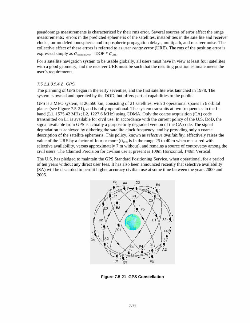
7-72
pseudorange measurements is characterized by their rms error. Several sources of error affect the rangemeasurements: errors in the predicted ephemeris of the satellites, instabilities in the satellite and receiverclocks, un-modeled ionospheric and tropospheric propagation delays, multipath, and receiver noise. Thecollective effect of these errors is referred to as user range error (URE). The rms of the position error isexpressed simply as σPosition Error = DOP * σURE.
For a satellite navigation system to be usable globally, all users must have in view at least four satelliteswith a good geometry, and the receiver URE must be such that the resulting position estimate meets theuser’s requirements.
7.5.1.1.3.5.4.2 GPS
The planning of GPS began in the early seventies, and the first satellite was launched in 1978. Thesystem is owned and operated by the DOD, but offers partial capabilities to the public.
GPS is a MEO system, at 26,560 km, consisting of 21 satellites, with 3 operational spares in 6 orbitalplanes (see Figure 7.5-21), and is fully operational. The system transmits at two frequencies in the L-band (L1, 1575.42 MHz; L2, 1227.6 MHz) using CDMA. Only the coarse acquisition (CA) codetransmitted on L1 is available for civil use. In accordance with the current policy of the U.S. DoD, thesignal available from GPS is actually a purposefully degraded version of the CA code. The signaldegradation is achieved by dithering the satellite clock frequency, and by providing only a coarsedescription of the satellite ephemeris. This policy, known as selective availability, effectively raises thevalue of the URE by a factor of four or more (σURE is in the range 25 to 40 m when measured withselective availability, versus approximately 7 m without), and remains a source of controversy among thecivil users. The Claimed Precision for civilian use at present is 100m Horizontal, 140m Vertical.
The U.S. has pledged to maintain the GPS Standard Positioning Service, when operational, for a periodof ten years without any direct user fees. It has also been announced recently that selective availability(SA) will be discarded to permit higher accuracy civilian use at some time between the years 2000 and2005.
Figure 7.5-21 GPS Constellation

7-73
7.5.1.1.3.5.4.3 GLONASS
Russia's GLONASS consists of a series of 24 MEO satellites in 3 orbital planes (see Figure 7.5-22) at25,510 km providing navigational and accurate global positioning services (claimed precision: Horizontal= 100m; Vertical = 150m). The first GLONASS was launched in December 1980. The constellationremains sparsely populated (twelve active satellites on average for the past few years), and political andeconomic difficulties in Russia continue to be a source of uncertainty about its future.
GLONASS uses FDMA in the 1602 - 1615.5 MHz band. The service interferes with the radio astronomyband (1610.6-1613.8 MHz), and with the recently allocated mobile satellite service at 1610-1626.5 MHz.An L1 and L2 organization, with CA code for civilian use was adopted - similar to GPS. AlthoughGLONASS officially disavowed a selective availability-like feature (σURE = 10 m), its positioningspecifications are almost identical to those of GPS.
Figure 7.5-22 GLONASS Constellation
7.5.1.1.3.5.4.4 Differential GPS
Differential GPS (DGPS) is the regular GPS with an additional correction (differential) signal added.This correction improves the accuracy of the GPS and can be broadcast over any authorizedcommunication channel. DGPS receivers collect navigational information signals from all satellites inview, plus differential corrections from a DGPS station in the area. (Many DGPS receivers consist of twounits: a GPS receiver, with a data port for DGPS corrections directly connected to a radio receiver.)
The Coast Guard is developing a DGPS service for public use in harbor and harbor approach areas, aswell as in the Great Lakes, most of Alaska, Hawaii, and Puerto Rico. DGPS uses pseudorange correctionsbroadcast over the existing network of marine radio beacons. The Coast Guard plans to complete thesystem and declare it operational in 1996.
7.5.1.1.3.6 Assessment for ITSSummarizing now the technology assessment of satellite systems, it can be safely stated that the proposedand already deployed systems guarantee a wealth of choices for the provision of those ITS services thatcan not be provided by cheaper, more effective means, like two-way cellular. The user must moderate

7-74
any optimistic expectations about service availability, given the huge investments required by most of theproposed systems in the face of market uncertainties, as well as their complexity and deployment risk.
7.5.1.1.4 Meteor Burst CommunicationsThe meteor burst (or meteor scatter) channel, known as the “poor man’s satellite channel”, relies on theionized trails of meteors as reflectors to achieve long range packet data communications. It was foundthat useful ionized meteor trails occur at an altitude of about 80-120 km above the earth’s surface. Trailswith useful electron densities for reflecting radio signals in the range of 40 to 50 MHz were found to beplentiful enough to provide communications over a range of roughly 2000 km. The minimum rangelimitation was found to be 400 km, as determined by the scattering geometry and electron density. Theintermittent nature of the channel has to do with the random distribution of the meteors of interest whichshows a strong diurnal variation (peaking at 6:00 local time, and with a distinct minimum at 18:00), andfollows the Poisson law. Ionized trails were found to have a lifetime of only a few tenths of a second,creating the need for rapid exchange of information (thus the term “burst communications”). Due to theunique characteristics of the propagation mechanism (see Figures 7.5-23 and 7.5-24), Meteor BurstCommunications relies on an inherent spatial multiplexing to reduce the contention in a network withpotentially more than ten thousand units.
Ionization RegionsTime 1
Time 3Time 2
Receivers located within Trail Footprint
Receivers illuminated at Time 1 Time 2
Figure 7.5-23 Motion of Ground Illumination Region due to Trail Formation and Decay
LongMedium
Small
Transmitter Receiver
Figure 7.5-24 Effect of Trail Location on Size of Footprint

7-75
A system with the characteristics described above seems appropriate for communicating with remote,usually rural, sparsely populated areas, when there is no need for immediate, urgent communications.The coverage of conventional UHF cellular systems is too small for cost effective seamless coverage invery rural areas, especially away from major interstate highways. On the other hand, satellite service isvery expensive to install and operate. Meteor Burst technology costs approximately 1/5 that of satellitesystems, and the long term life cycle costs savings can not be underestimated (meteors are in essence freenatural satellites, always available). Furthermore, since Meteor Burst operates in the low VHF band, thecost of the vehicle radio equipment is approximately half that of corresponding satellite equipment.
Examples of ITS services that a Meteor Burst system could potentially support are wide area AutomaticVehicle Location (AVL), and remote (long haul) Fleet Management. Surveys of potential users indicatethat when out on the open road, position information every 10 to 15 minutes with short messagecapabilities is adequate for significant productivity enhancement. A Meteor Burst tracking system can fillthe gap in the conventional cellular system where in remote areas the density of vehicles (and fixedusers) cannot justify the base station infrastructure.
A Meteor Burst system could provide seamless coverage of the continental U.S. with as few as 100 basestations. However, noise levels in urban areas are too high for Meteor Burst usage. There, cellularcoverage would have to be considered, pointing to the possibility of dual MB-cellular systems.
Several Meteor Burst systems have already been installed and proven effective:
• In the 1950’s, Canada installed the JANET system between Toronto and Port Arthur for simple pointto point teletype communications.
• Also in the 1950’s, SRI, under contract from the U.S. Air Force, operated a test link from Palo Alto,CA to Bozeman, Montana, primarily for propagation research.
• The 60’s saw the first operational military MB communication system deployed in Europe, calledCOMET, operated by the NATO SHAPE technical center, providing communication from TheHague, Netherlands, to southern France, again to transmit conventional teletype messages.
• In the late 70’s, the Alaska SNOTEL (for SNOwpack TELemetry) system was installed to providemeteorological information from remote locations throughout Alaska.
• The Alaska National Guard recently installed a MB system that ties headquarters to remote locationsthroughout the state.
• A MB system has been installed between Sondstrom AB and Thole AB, Greenland.
• MB was selected for the Small Mobile ICBM (SICBM) program to provide primary communicationunder almost all conditions between mobile launch control centers and up to 1000 mobile launchersrandomly dispersed over a wide area.
• Currently NORAD is testing a C3 MB network that will connect the continental US, Alaska, andCanada.
As for commercial systems, a few experiments have been successful, namely one in the Portland, ORarea where a long haul Fleet Management system has been deployed, taking advantage of the MB beyondline of sight communication capabilities.
As a conclusion, MB, although requiring a dedicated system, seems to be a cheap but still effectivealternative to expensive satellite systems. In any circumstance, it cannot provide overall seamlesscoverage, thus requiring terrestrial cell-based coverage in urban and suburban areas in a dual MB-cellularsystem configuration.

7-76
7.5.1.1.5 Broadcast SystemsIn the area of ITS broadcasting there are presently as many as three different high data rate FM subcarriersystems in contention for national acceptance, while RBDS is already standardized (and available) forlower data rates.
Although we will focus primarily on FM subcarrier systems, other broadcast techniques will also beconsidered to determine their applicability to the ITS services. These technologies vary considerablyfrom the simple, such as HAR, to the more advanced like DAB and transmission within the TV verticalblanking period, or to using a whole SAP sub-channel. We will address also the most promising of theseother technologies.
The level of detail of the analysis will be determined by the anticipated ITS role. As applicable, thecapacity of the above systems will be determined, as well as the information update rates allowed.
7.5.1.1.5.1 Operational EnvironmentThe typical environments that broadcast systems will operate in include rural, urban, suburban and inter-urban areas. The received signal will experience propagation effects such as blockage and multipath, andthe success of a broadcast system will depend on its effectiveness in defeating those effects.
The propagation anomalies are primarily dependent on the operational environment, such as the type ofthe natural and man made structures, e.g., hills and buildings. Furthermore, the climate, the vegetation, aswell as the materials of the obstacles will also affect the propagation environment. The other variable thatchanges the propagation environment is the driving conditions. For example, when driving in the citythere will be frequent blockage periods due to buildings, hence system performance will be a function ofthe driving speeds, and would be quite different for speeds that range from 0 to 70 mph.
Broadcast propagation environment, and the ability of the broadcast systems to mitigate its effects will bea key parameter in identifying the appropriate ITS services that can be supported using a particularcommunication technology. For example, there will be broadcast systems that will transmit messages atregular intervals, such as bus schedules and weather forecasts, and others that will transmit only atspecific times (e.g. hourly news). Therefore, the loss of information due to blockage and multipath willbe of a lesser significance for some services and of a greater significance for others.
By definition, broadcast systems are not suited for two-way communication. One can only envision theiruse in very specific applications of ITS (e.g., transmitting traffic status information both on the freewaysystem and on surface streets - a value added service that may be of interest to some broadcasters). Thiswould require, however, coordination with (or by) the control centers, and the definition of strict receiverstandards to minimize the cost associated with the display of information.
Moreover, as already stated, the most critical performance limitation of Subcarrier Authorization (SCA)arises from multipath, or fading in general. Unfortunately, in the ITS environment multipath isunavoidable if one wishes to employ simple, cheap antennas (e.g., whip or monopole antennas). Undermobile conditions, it is not possible, without incurring unacceptable receiver costs, to try to compensatefor, or nullify, the multipath effects. Thus, the broadcast system must either be designed such that itaccounts for the degradation caused by the multipath, or by explicitly taking into account that sometimesthe receiver will not be able to properly receive the information.
A possible operational solution would be to continuously repeat the traffic status information, updating iton the run. If a vehicle is unable to receive traffic information for a while due to specific propagationconditions, it would rely on the last successfully received status report, which would be updated as soonas reliable reception resumes.

7-77
Another possible (possibly simultaneous) solution would be to provide alternative sources of information(other radio stations) providing the same traffic information, conveniently offset in time. This wouldnecessitate a more complex (costly) receiver that would automatically switch from a “bad” to a “good”station.
7.5.1.1.5.2 Evaluation ApproachThe goal of this technical evaluation is to analyze the capabilities of the existing and projected broadcasttechnologies in the context of the National ITS architecture. The analysis will utilize the requirements ofthe ITS services and communication links that are suited for one-way wireless dissemination, and theircritical attributes, such as message sizes, information rates, frequency of use,, etc. The results of the ITSbroadcast data loading analysis of Section 5.2 will be applied in the evaluation.
The analysis will address the following issues and parameters:
1. Data rate for high and low data rate broadcast systems. Includes overhead for error correctionand multipath mitigation (coding, interleaving, repeat broadcasting, etc.).
2. Message delivery delay.
3. Modulation techniques.
4. Coding and interleaving techniques for defeating channel errors.
5. Approach for mitigating mobile channel effects (e.g., multipath) These techniques include: (1)complex coding and interleaving, (2) combined modulation and coding, and (3) simple codingand interleaving with a repeated transmission algorithm.
6. The capacity of the broadcast system as a function of the message sizes and update frequency.The capacity and update frequency are inversely proportional, for a fixed information rate (i.e.,as the requirement for the update frequency increases the effective capacity of the broadcastsystem decreases).
7. The data processing in the mobile units. It is an important consideration when evaluating theservices that can be supported using broadcast techniques. This capability will allowbroadcasting only the minimum amount of data (e.g., broadcasting compressed trafficinformation, instead of detailed information).
8. System coverage will be a function of the broadcast tower locations, and will also depend on thedeployment strategy. The systems can use one or multiple frequencies for broadcasting. Thereare two options when using multiple stations (frequencies): (1) The stations can broadcast thesame information with staggered repeat, which reduces message delivery delay at the cost of lostcapacity; or (2) the stations can broadcast different information, therefore maximizing capacity.
9. System reliability. The effective broadcast data rate is reduced due to the reliability factor, as aresult of system failures and propagation effects (e.g., blockage, multipath, etc.). A reliabilityfactor of K% (e.g., 90% effective throughput) will be included in the analysis.
10. Addressing capabilities; the capability of addressing specific customers.
11. Interface issues: open versus proprietary interfaces.
12. Deployment cost.
In what follows the above issues will be addressed in some detail. Furthermore, the proposed andoperating systems will be described and their specifications will be summarized. The analysis will

7-78
include field test results, when applicable. The field test results address issues related to deploymentstrategies, implementation, cost, candidate services, available hardware and terminals, and serviceprovision.
7.5.1.1.5.3 FM SubcarrierIn Europe, the spectrum allocation for FM stations is 150 kHz, while in North America it is 200 kHz. Theinternational CCIR standard allows a subcarrier frequency of 53 to 75 kHz, while the North Americanstandard allows for 53 to 99 kHz.
In recent years the FCC allowed for the opening of the FM baseband to 99 kHz, and relaxed the technicalusage rules. This stirred up great interest in new services via SCA, e.g., teleprinter newscasting, computerdata transmission, and paging. SCA allows for the use of the spectrum not occupied by the FM-stereochannel, provided certain conditions of non-interference with the audio channel are met. Deregulationhas removed all restrictions on allowable modulations.
Figure 7.5-25 illustrates the FM baseband and subcarrier spectrum. Each FM station is allocated a 200kHz bandwidth for transmitting the FM signal. In Figure 7.5-25, the baseband bandwidth between 53 and100 kHz is not used for transmitting a stereo music signal, and can be used for broadcasting auxiliaryprograms and data. FM stations have the authority under their license to broadcast auxiliary programsand data without further permission from the FCC.
.005 15 19 23 53
L+R L-R
100 %
10 %
% o
f Mod
ulat
ion
of C
arrie
r
Frequency (kHz)
EuropeanStation SpectrumLimit
North AmericanStation SpectrumLimit
75 99
Subcarrier Authorization
Figure 7.5-25 FM Spectrum Allocation in North America and Europe
The U.S. has adopted the international standard for transmitting low data rate using the FM subcarrier atthe baseband frequency of 57 kHz (this is at three times the FM pilot of 19 kHz). This system is referredto as the Radio Broadcast Data System (RBDS). As a result, in order to insure co-existence of RBDSwith high speed FM subcarrier systems, they are restricted to using the spectrum above 60 kHz (seeFigure 7.5-26).

7-79
L+R L-R
Pilot
RBDS57 kHz
19 kHz 100 kHz
High data ratesubcarrier bandwidth
Figure 7.5-26 FM Baseband Spectrum (Not to scale)
The two most important problems inherent to FM subcarrier operation are crosstalk and the “birdies”effect. Crosstalk is the effect on the FM subcarrier channel of interference from the FM stereo channel,and it almost entirely determines the noise performance of the FM subcarrier. It is obviously determinantwhen operating a data FM subcarrier channel. The so called “birdies” which appear in the main FMstereo channel are interference caused by the FM subcarrier channel(s). They consist of high frequencyaudio whistles, typically 5–10 kHz, that are frequency modulated by the FM subcarrier material. Thisproblem is solved in practice by the use of a PLL FM receiver for the case of a standard FM subcarrierchannel side by side with the main FM stereo channel.
Any proposed system must prove non-interference with the main FM stereo channel, as well as other FMsubcarrier channels.
7.5.1.1.5.3.1 Proposed and Existing FM Subcarrier Systems
There are a number of broadcast systems that are operational or have been proposed. The main differencebetween these systems is in their modulation techniques and the approach for mitigating the multipathand other mobile propagation problems, such as multipath and blockage. These systems use two distincttechniques for combating the propagation impairments. In the first approach, complex coding andmodulation formats are used, as in MITRE’s STIC and NHK’s DARC system. The second approach usestime and frequency diversity, for example multiple FM stations are used for frequently (e.g. twice everyfew minutes) broadcasting the same message. In the second approach the terminal captures the signalfrom the strongest broadcast station; SEIKO’s HSDS uses this scheme. These high data rate systems aredescribed in greater detail in the subsections to follow.
We begin with RBDS, the U.S. version of the European RDS standard. R(B)DS provides low data rateservice and is used, especially in Europe, to transmit traffic information without affecting the FM stereosignal.
7.5.1.1.5.3.1.1 RBDS and RDS-TMC
The Radio Data System (RDS) is an FM subcarrier standard first available in Europe and now gainingacceptance in the US under the acronym RBDS. RBDS uses bi-phase shift keying (BPSK) modulationformat for transmitting at a data rate of 1187.2 bps, occupying the bandwidth from 53.5 to 59.4 kHz. Theeffective information rate for RBDS is about 300 bps, considering the overhead of coding andinterleaving.
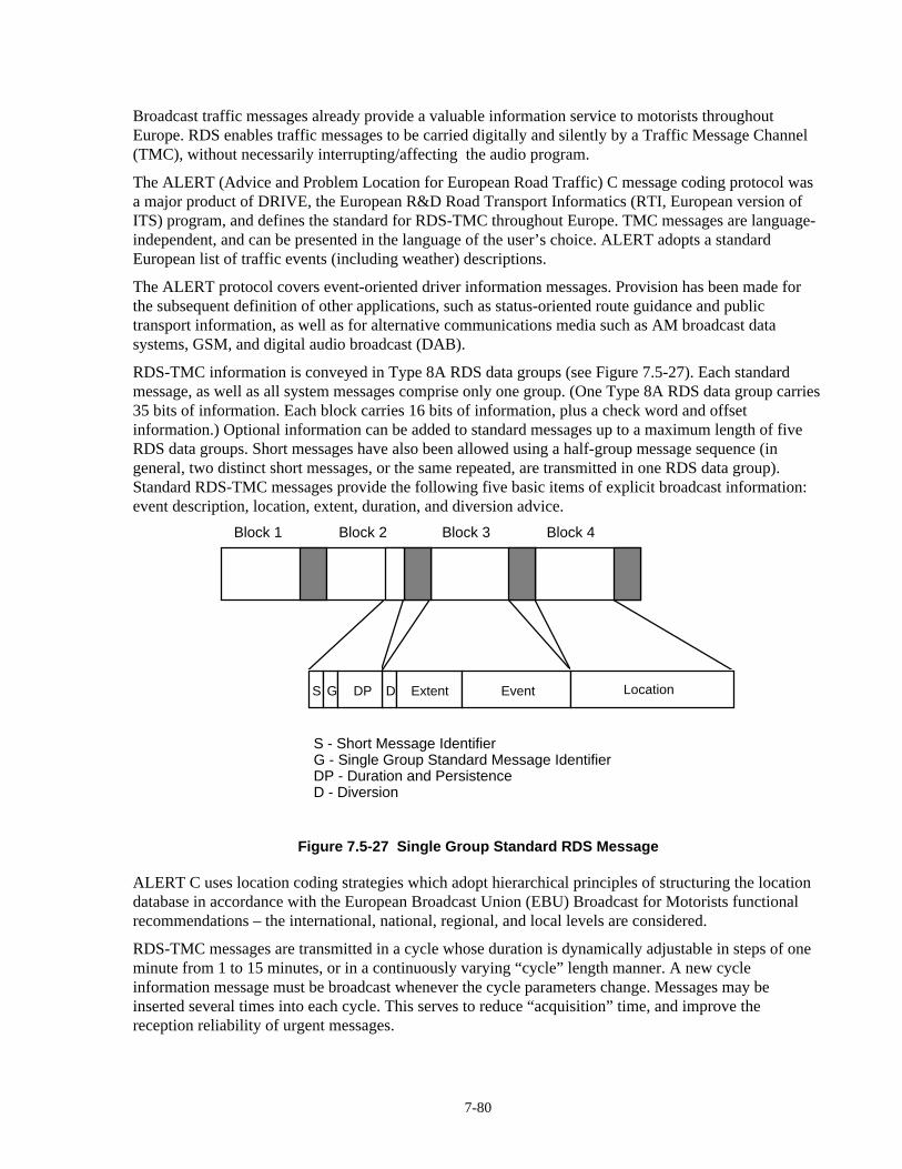
7-80
Broadcast traffic messages already provide a valuable information service to motorists throughoutEurope. RDS enables traffic messages to be carried digitally and silently by a Traffic Message Channel(TMC), without necessarily interrupting/affecting the audio program.
The ALERT (Advice and Problem Location for European Road Traffic) C message coding protocol wasa major product of DRIVE, the European R&D Road Transport Informatics (RTI, European version ofITS) program, and defines the standard for RDS-TMC throughout Europe. TMC messages are language-independent, and can be presented in the language of the user’s choice. ALERT adopts a standardEuropean list of traffic events (including weather) descriptions.
The ALERT protocol covers event-oriented driver information messages. Provision has been made forthe subsequent definition of other applications, such as status-oriented route guidance and publictransport information, as well as for alternative communications media such as AM broadcast datasystems, GSM, and digital audio broadcast (DAB).
RDS-TMC information is conveyed in Type 8A RDS data groups (see Figure 7.5-27). Each standardmessage, as well as all system messages comprise only one group. (One Type 8A RDS data group carries35 bits of information. Each block carries 16 bits of information, plus a check word and offsetinformation.) Optional information can be added to standard messages up to a maximum length of fiveRDS data groups. Short messages have also been allowed using a half-group message sequence (ingeneral, two distinct short messages, or the same repeated, are transmitted in one RDS data group).Standard RDS-TMC messages provide the following five basic items of explicit broadcast information:event description, location, extent, duration, and diversion advice.
Block 1 Block 4Block 3Block 2
S G DP D Extent Event Location
S - Short Message Identifier G - Single Group Standard Message Identifier DP - Duration and Persistence D - Diversion
Figure 7.5-27 Single Group Standard RDS Message
ALERT C uses location coding strategies which adopt hierarchical principles of structuring the locationdatabase in accordance with the European Broadcast Union (EBU) Broadcast for Motorists functionalrecommendations – the international, national, regional, and local levels are considered.
RDS-TMC messages are transmitted in a cycle whose duration is dynamically adjustable in steps of oneminute from 1 to 15 minutes, or in a continuously varying “cycle” length manner. A new cycleinformation message must be broadcast whenever the cycle parameters change. Messages may beinserted several times into each cycle. This serves to reduce “acquisition” time, and improve thereception reliability of urgent messages.

7-81
Message priority was another issue where the EBU Guidelines on Broadcasts for Motorists have beenfollowed, distinguishing mainly between strategic and tactical information. By definition, strategicinformation is of value for trip planning and route selection in the medium term, and tactical informationis likely to be of relevance for immediate local diversions around current traffic problems. The followingrange of broadcast message priorities are considered:
• Highest Priority -- for immediate broadcast, interrupting ongoing RDS-TMC message cycles, andbeing repeated frequently;
• Tactical Information -- for non-delayed broadcast through early insertion into RDS-TMCmessage cycles, with frequent repeats;
• Strategic Information -- broadcast at fixed intervals according to RDS-TMC channel capacity;and
• Background Information -- broadcast less frequently, when channel capacity permits.
From the above, necessarily brief description of the RDS-TMC system, we see that it is a very versatile,well thought of broadcasting protocol, whose limitations are its inherent one-way characteristics, and thelow data rate of 1187.5 bps.
7.5.1.1.5.3.1.2 Modulation Sciences’ SCA
In this section, we analyze the system proposed by Modulation Sciences, Inc.10, one of the companiesinvolved in FM subcarrier. Error! Reference source not found. shows the proposed use of spectrum.The basic SCA channel audio response is 50 Hz to 5 kHz, with 0-20 Hz sometimes available for lowspeed telemetry applications. Restricting the maximum modulation frequency to 5 kHz guarantees abandwidth of 20 kHz for the SCA channel (in fact, the SCA channel bandwidth is only 14 kHz since theouter 3 kHz fall bellow the -25 dB threshold established by the FCC — that is why the upper SCAchannel could be centered about 92 kHz). The lower SCA channel is compatible with the Europeanstandards, while the upper SCA channel can only be used in North America. (The two-SCA channelstructure shown does not necessarily imply that one could not use the whole 53-99 kHz band to transmitdata.)
The established use of SCA has been in stationary applications. The problems identified in this sectionlimit SCA performance even in the stationary environment. Under mobile conditions, where thepropagation conditions are significantly more severe, more problems and limitations will certainlydevelop.
10Eric Small, “Data SCA: Some Real World Experiences”; Eric Small, “Making SCA work in the Real World”, Modulation
Sciences, Inc.

7-82
.005 15 19 23 53 57 77 82 10267 92
L+R L-RSCA Channels
100 %
10 %
% o
f Mod
ulat
ion
of C
arrie
r
Frequency (kHz)
EuropeanStation SpectrumLimit
North American Station Spectrum Limit
75 99
Figure 7.5-28 SCA FM Spectrum
7.5.1.1.5.3.1.2.1 Data SCATwo types of data modulation have been considered for data SCA transmission, namely Direct andIndirect Data Modulation. In Indirect Data Modulation, also known as Compatible Modulation, the signalthat goes into the SCA generator is a sequence of audio tones (AFSK). The advantage of this type ofmodulation is that standard (i.e., no-data) SCA generators can be used unmodified; thus cheap and easyto use generators are available. Disadvantages are the slow data rates that can be accommodated (lessthan 1200 bps), and the relatively expensive demodulator required to turn the audio back into data.
By switching the phase of an audio tone instead of its frequency, higher data rates can be achieved, butthe cost of the receiver demodulator rises very rapidly with data rate, and, conversely, the tolerance of thesystem to interference (crosstalk) drops quickly. The advantage of this technique is that it employs thesame technology used to send data via the telephone network; thus hardware is generally available, and iswell understood. Usually data rates are bellow 9.6 kbps.
Direct Data Modulation takes advantage of something available to the FM subcarrier user, namely thesubcarrier itself. The SCA subcarrier (at 67 or 92 kHz) is available for direct manipulation by thebroadcaster. Instead of varying the frequency of an audio tone that in turn modulates the SCA subcarrier,the carrier itself is modulated. Higher data rates can be achieved with less bandwidth, and the receiverdemodulators are cheap too.
Direct Data Modulation uses either MFSK, varying the frequency of the carrier itself, or MPSK, varyingthe carrier’s phase. MPSK, however, requires a phase reference. Luckily, in FM stereo, an ideal externalphase reference already exists: the 19 kHz pilot. A data rate of up to 46 kbps can be achieved withMPSK, occupying the entire SCA portion of the FM channel, from 53 to 99 kHz, but requiring arelatively expensive receiver. As a comparison, Modulation Sciences’ Data Sidekick system achieves4800 bps at a measured BER of 10-7 for fixed links under “good” weather conditions.

7-83
In fact, the first and foremost problem of SCA, the one that limits the data rate, is multipath. Under fixedconditions, using appropriate antennas allows mitigation of the multipath to assure almost always a givenBER. The biggest problem, even then, remains that of “equalizing” or “zeroing” late/undesirablereflections. (Especially in urban environments, the reflection coefficient in masonry varies widely, asmuch as 25 dB, depending upon its surface being wet or dry.)
7.5.1.1.5.3.1.3 SEIKO’s High Speed FM Subcarrier Data System (HSDS)
SEIKO® Telecommunication Systems, Inc. (STS) has developed a flexible High Speed FM subcarrierData System, known as HSDS, with a capability for world wide operation. HSDS is a fully developedone-way system providing messaging and information services (e.g., personal messaging, trafficinformation, time of day, news, weather, sports, business, and emergency information). The system hasbeen deployed by STS under the Receptor™ trade mark in a number of cities (Portland, OR in 1990;Seattle-Tacoma, WA in 1992; Los Angeles, San Francisco, CA in 1995; a few East Coast cities in 1996).Coverage maps for some of these areas are shown in Figures 7.5-29 and 7.5-30.
Figure 7.5-29 HSDS Coverage in the Southern California Area for Wrist-Watch Receiver (-29 dBi antenna)

7-84
The philosophy of the system design and operations is:
• The information is cyclically repeated at a rate of a few transmissions every 2-3 minutes.Therefore, if a user misses the information the first time due to blockage or error he/she willeventually receive it on the succeeding transmissions.
• The complexity of the handset is low. This has been achieved by using simple modulation andcoding schemes, and using space, time and frequency diversity for mitigating multipath.
The HSDS utilizes existing FM radio broadcasting infrastructure, currently available IC’s andtransmission equipment, making it relatively inexpensive to deploy. By design it permits very small
receivers: alphanumeric display wrist-watch receivers (SEIKO® Receptor™ MessageWatch™ whichsells for $75-150), and pocket pagers. Receivers with duty cycles varying from 100% to less than 0.01%provide flexibility to select message delay, data throughput, and battery life.
The HSDS can operate as a stand alone single station system, or as multiple systems operatingindependently in a geographical area with each system including multiple stations. Multiple stations areaccommodated by frequency agile receivers, time offset message transmission in each station, andtransmitted lists of stations surrounding each station (three FM stations provide coverage for 1.2 millionpeople in Portland, OR; seven FM stations provide a coverage area with 2.6 million people in Seattle-Tacoma, WA).
Figure 7.5-30 HSDS Coverage in the Portland, OR, and Seattle, WA, Areas for Wrist-WatchReceiver (-29 dBi antenna)
7.5.1.1.5.3.1.3.1 HSDS Technical SpecificationsThe HSDS system is time division multiplexed. Time is subdivided into a system of master frames, sub-frames and time slots. Each slot contains a packet of information. In multiple station systems, each

7-85
station’s transmissions are synchronized to UTC ensuring synchronization between stations. Thesynchronized and time offset stations provide an opportunity to change the tuned frequency and makesubsequent attempts to receive packets on other available frequencies.
Each receiver is assigned a set of slots as times for monitoring transmissions. (Multiple receivers mayshare time slots, due to the random nature of expected communications.) Each slot is numbered and eachpacket contains the slot number to permit rapid location of assigned time slots.
The error correction scheme is flexible, the methods used varying with the application. The method usedfor wrist-watch reception is designed to correct a short burst of errors associated with random noise orautomotive ignition noise. The standard CCITT 16 bit CRC is typically added as a component of eachpacket, and minimizes the chances of “missed” packets.
HSDS’ modulation/encoding provides high data rate, narrow bandwidth with high spectral efficiency (1bit/s/Hz), and negligible impact on the main audio channel, or on any existing RBDS subcarrier. The
HSDS modulation is DSB SC AM with duobinary encoding11; the data rate is 19 kbps in a 19 kHzbandwidth centered at 66.5 (=3.5 x 19) kHz. The HSDS signal is modulated as a subcarrier ranging from5% to 20% -- typically at 10% on commercial FM radio stations. Sharp transmission filter skirts causeextremely little impact on the main audio channel in no multipath conditions; generation of a randomizeddata stream reduces the impact of multipath. The narrow bandwidth of HSDS allows for compatibilitywith RDS operation world wide. Furthermore, from Figure 7.5-31, HSDS allows for use of subcarriersabove 76 kHz in the US, and compatibility with European spectral allocation.
L+R L-R
Pilot
RBDS57 kHz
19 kHz 100 kHz
High SpeedSubcarrier Data Systems
66.5 kHzHSDS #1
85.5kHzHSDS #2
16 kHzOccupied BW
Figure 7.5-31 FM Baseband Spectrum usage for Seiko’s HSDS System
The effective information rate for HSDS system is 7500 bps (considering coding and repeat transmissionoverhead). The HSDS system transmits 72 packets of data per second, where each packet of data contains104 bits of information. To reduce the impact (interference) on the audio channel, HSDS uses sharp skirtfilters in addition to randomizing the data using PN sequences. As a result the data looks like randomnoise. A typical packet of data is first Encoded, then Randomized, and finally Interleaved .
SEIKO’s HSDS system multiplexes data streams of varying bandwidths. As the transmission begins,bandwidth is dynamically assigned and subscribing receivers are alerted to the service. This bandwidth is
11 A. Lender, “The Duobinary Technique for High Speed Data Transmission”, AIEE Trans. Commun. Electronics, 1963.

7-86
then freed at the conclusion of the data stream transmission. Multiple data streams may be carriedconcurrently with small packet-oriented transmissions (such as paging and messaging).
7.5.1.1.5.3.1.3.2 Multipath and Shadowing Mitigation StrategyRobust wireless systems require methods to address multipath and shadowing. Some systems attempt toaddress these issues with extensive error correcting schemes. While these techniques are useful for themoving receiver, they become ineffective when the receiver is stopped in an extremely low signalstrength area, or moving very slowly through multipath nulls. Diversity techniques are frequently used tocombat fading effects.
HSDS addresses multipath and shadowing with a combination of frequency, space, and time diversity,and message numbering. Frequency diversity is achieved through frequency agile receivers (87.5-108MHz). Space diversity (multiple station systems) provides paths from two or more directions reducingthe size of shadowed areas, and the possibility of missed messages.
Time diversity can be provided in two ways: multiple transmissions on the same station, and delayedtransmission between stations. Duplicated messages are rejected via comparison with the transmittedmessage number. Multiple transmissions of information several minutes apart are utilized for wristmobile applications.
7.5.1.1.5.3.1.3.3 HSDS versus RDS-TMCA comparison with RDS-TMC, in particular with the RDS-ALERT C protocol, is warranted. From Table7.5-10, we see that there is indeed a big difference in data rate in favor of HSDS. On the other hand, thecycle length is fixed for HSDS, although as we have seen, messages can be repeated within a cycle. Inany case, HSDS seems to be a promising alternative to RDS-TMC.
Table 7.5-10 Comparison of HSDS and RDS-TMC
Center Frequency
(kHz)
Bandwidth
(kHz)
Raw Data Rate
(bps)
Cycle Length
RDS-ALERT 57 4.8 1187.5 Variable
HSDS 66.5 19 19000 Fixed
Although HSDS requires a reasonably inexpensive infrastructure, and relatively inexpensive, smallreceivers, it is still a proprietary one-way system. Nevertheless, it appears to be a promising substitute forlower rate R(B)DS systems.
7.5.1.1.5.3.1.4 MITRE’s Subcarrier Traffic Information Channel (STIC)In early 1992 FHWA sponsored a research and development project for developing a high data ratesubcarrier technology. MITRE/FHWA developed a high data rate subcarrier data system, andimplemented a proof-of-concept prototype. The system is called Subcarrier Traffic Information system(STIC). STIC uses a complex data, and modulation format for defeating the multipath and otherpropagation effects. The prototype of the STIC receiver was tested in the Fayetteville, NC. The results ofthis trial were not available at the time of this writing.

7-87
7.5.1.1.5.3.1.4.1 Technical SpecificationsFigure 7.5-32 illustrates STIC’s baseband spectrum.
L+R L-R
Pilot
57 kHzRBDS
19 kHz 100 kHz72.2 kHzSTIC
16 kHzOccupied BW
Figure 7.5-32 FM Baseband Spectrum Usage for MITRE’s STIC System
The STIC data format first uses convolutional encoding, and interleaving. The interleaved data blocks arefurther processed by appending to each block 4 channel state estimation bits. This data is then BCHencoded and followed by the π/4 DQPSK modulator. The modulated signal is further filtered using thesquare root raised cosine filer with a roll-off factor of 0.68.
The parameters of the interleaver and coding are designed based on the propagation data in the FM band(100 MHz). The achievable information rate is 8 kbps, this is for a typical BER of 10-5 . The raw symbolrate for STIC is 18.8 kbps.
The propagation parameters are a key element in selecting the parameters of the STIC waveform, such asthe interleaver size, number of channel state bits, and encoding techniques. The typical values that havebeen considered for the evaluation phase are:
• Delay = 3 x 10⁻⁶ sec.
• Doppler spread of 8 Hz (at 55 mph for the 100 MHz band)
The complexity of the receiver will depend on the above parameters. STIC mitigates the propagationeffects by using the channel state information to estimate the quality of the received data, therebyenhancing the decoding algorithm.
7.5.1.1.5.3.1.5 NHK’s Data Radio Channel (DARC) System
The Digital DJ Inc. and NHK of Japan are partners in developing the FM Subcarrier InformationServices (FMSIS) for US applications. This system uses the data radio channel (DARC) technologydeveloped by NHK Laboratories for broadcasting 16 kbps data using the FM subcarrier. DARC uses thelevel controlled minimum shift keying (L-MSK) modulation format, which is a variation of MSK. Thismodulation format has proven to be robust in a multi-path environment.
The level of the multipath in an FM subcarrier digital data system is related to the magnitude of thestereo sound level. At low stereo sound signal levels the multipath levels will be negligible when usinglow injection levels for the data signal. However, in the presence of higher stereo sound levels, injection

7-88
levels of 10% are required. By using L-MSK, which increases the injection level only during an increasein the sound level, the digital signals are transmitted efficiently under multipath conditions. Furthermore,DARC employs two dimensional CRC coding to correct channel and burst errors.
7.5.1.1.5.3.1.5.1 DARC Technical SpecificationsThe FMSIS, using the DARC modulation format, places the digital data at 76 kHz baseband frequency, ata data rate of 16 kbps. This results in an occupied bandwidth of about 32 kHz. DARC’s effectiveinformation rate, after error correction, is about 8 kbps or about 1,000 alphanumeric characters persecond. The system is designed to co-exist with the low data rate RBDS system (Figure 7.5-33). Thereliability of the system (% of correct reception) is improved by repeat broadcasting at a rate of 2 to 3times every few minutes.
The receiver for the DARC system uses a chip set, developed by SANYO, for (1) filtering, (2) L-MSKdemodulation, and (3) synchronization and decoding. The receivers will incorporate the chip sets todecode the received data and display the information using LCD panels.
L+R L-R
Pilot
RBDS57 kHz
19 kHz 100 kHz76 kHz
FMSS signal
about 32 kHzOccupied BW
Figure 7.5-33 FM Baseband Spectrum Usage for NHK’s DARC System
7.5.1.1.5.3.1.5.2 Field Test ResultsIn September of 1993 the DARC system was tested in Tokyo, using first generation receivers. Theparticipants included both auto and radio receiver manufacturers. The trial included propagation testunder (1) multipath conditions, (2) normal road, and (3) highway conditions. The results of this testpresented the system bit-error-rate, and were used to estimate the system reliability (% of correctreception), under various conditions. The reported results claim reliability of 90 to 95% that can beobtained when using multiple repeat techniques.
In summary, DARC resorts to a more complex mobile unit, and lower per transmitter capacity to providegains in reliability.

7-89
7.5.1.1.5.3.2 Evaluation Results and Conclusions
7.5.1.1.5.3.2.1 Capacity Analysis ResultsThe capacity of the broadcast systems is analyzed in the context of the ITS Architecture using the dataloading analysis in Chapter 6 supported by Appendix F. The summary of these results is depicted inTable 7.5-10. The results present the aggregate information rate for traffic information services, travelinformation services and transit information services. The aggregate information rate is further evaluatedfor a growth rate of 10, 20 and 30 percent. The growth rate includes the increase in the number of linksand the increase in the required update rates.
Table 7.5-10 presents the capacity of the high data rate FM subcarrier systems, viz., HSDS, DARC, andSTIC, using a single and dual broadcasting channel. The capacity for these systems is evaluated at thethree reliability factors of 100, 90, and 70 percent. The reliability factor accounts for the propagationimpairments, such as holes in the coverage, multipath, blockage, etc. These results are presentedassuming a single station operation, i.e., that if more than one station is used they do not supplement eachother to increase reliability.
From Table 7.5-10, it is observed that the high data rate FM broadcast systems can meet the capacityrequirements of the proposed ITS services which are presented in Section 6. Since the RBDS system andhigh data rate systems can co-exist, if desired, the RBDS system can also be used to support either alimited number of services or lower information update rates.
Table 7.5-10 ITS Required Information Rates and Broadcast Systems Capacity
ITS Services Informationrate per ITS
service (bps)
Increase in informationrate due to demand
High data rate broadcast systemcapacity
effective information ratesingle channel
at a reliability factorof
dual channelat a reliability
factor of10% 20% 30% 100% 90 % 70 % 100 % 90 % 70 %
Traffic informationservices
1,366 1,502 1,639 1,775
Transit services 1,536 1,690 1,843 1,997
Traveler InformationServices
2,750 3,025 3,300 3,575
Total BroadcastInformation Rate
5,651 6,217 6,782 7,347 7,500 6,750 5,250 15,000 13,500 10,500
7.5.1.1.5.3.2.2 Coverage and Deployment Issues
The first approach to propagation mitigation uses multiple broadcast stations (i.e., multiple frequencybands), for transmitting the same information. Evidently the location of the FM towers in this case is ofprimary importance in optimizing the coverage area. The potential increase in the coverage area willresult in an effective lower system capacity, since the same message will be broadcast from multiplestations. In this approach, the receivers will have the capability of tuning to multiple stations andselecting the strongest signal.
In the second approach, the broadcast system uses coding and modulation techniques for multipathrejection (STIC, DARC). Therefore, in general one FM station will be utilized per geographic area, tooffer a certain set of services. However, these systems require receivers of higher complexity, comparedto the first approach. In the complex mobile receiver approach the broadcast coverage could possibly beless than the first case, depending on the operational environment.

7-90
From the above discussion, the coverage and deployment, which are interrelated, depend on:
• The propagation environment – is one or multiple stations needed to meet the coveragerequirements?
• The required capacity – are multiple stations needed to meet the capacity requirements?
• Available broadcast systems (number of the available FM subcarrier systems).
The coverage area can be determined and optimized by selecting the broadcast technology (i.e., RBDS,HSDS, STIC or DARC) that will best meet the capacity requirements and best fit urban propagationconditions.
7.5.1.1.5.3.2.3 Interface IssuesThe core of the FM subcarrier broadcast systems is the algorithm required for demodulation, encodingand multipath mitigation, and the hardware/firmware that it requires. The broadcast system developershave been integrating the receivers into a set of LSI chips for compact implementation. The issues thatare involved in using broadcast systems include: (1) interface standards for inter-operability andnationwide compatibility, (2) licensing agreements for using the specific broadcast technology i.e.,hardware and software, and (3) system integration, i.e., hardware interface with ITS user terminals
With the exception of the low data rate RBDS system that has an open and standard interface, all highdata rate systems have proprietary interfaces (Table 7.5-11)
7.5.1.1.5.3.2.4 ConclusionsTable 7.5-11 outlines the broadcast technologies’ attributes. The high data rate FM subcarriertechnologies that were analyzed in this document will meet the capacity requirements of the ITS dataflows proposed for broadcast communication services.
The above analysis has also discussed the issues related to the coverage, interfaces, and national inter-operability. All high data rate systems that are discussed in this document (HSDS, STIC, and DARC)use proprietary hardware and interfaces, whereas RBDS uses a standard open interface. Using a systemwith a proprietary interface will impact the national inter-operability for the ITS services. The main issuein using a proprietary system will be the licensing agreements for the specific technology and hardware.
Table 7.5-11 Summary of the Broadcast System Specifications
BroadcastSystem
Status /Technology
Maturity
Interfaceissues
Implementation
Special Features &Tech. for combating
channels effects (e.g.,multipath)
Data Rate Inf. Rate
RBDS Operational /Commercial
Open Commercial 1187 bps 300 bps
STIC Prototype/Ready fordeployment
Proprietary,licenced forfree in U.S.
Prototype Uses coding, interleaving& correlation techniques.
18.8 kbps 7.6 kbps
DARC Operational /Commercial
Proprietary Commercial 19 kbps 8 kbps
SEIKO, HSDS Operational /Commercial(Oregon, LA,Seattle)
Proprietary Commercial Freq. and time diversity:scans for 7 Station,multiple transmission ofthe message, time offsetbetween stations
19 kbps 7.5 kbps
Note: RBDS can co-exist with High Speed FM subcarrier systems.
7-91
The main issue in deploying FM subcarrier systems will be the need for standardizing the interface withITS and achieving inter-operability between competing proprietary systems. Work is ongoing tostandardize the high speed FM subcarrier systems. The work involves independent assessment of thethree high speed systems, STIC, HSDS, and DARC, including their protocols and interfaces, by EIA atthe NASA Lewis Research Center.
A subset of the ITS services that will not require high data rate can be broadcast using RBDS. SinceRBDS has been standardized, those ITS services could easily achieve national inter-operability.
7.5.1.1.5.4 Digital Radio Broadcasting (DRB)The 1992 World Administrative Radio Conference (WARC-92) decided the world-wide allocation forDigital Radio Broadcasting (DRB) in L-Band.
DRB will replace both FM and AM stations. For FM stations, the plan should accommodate DRBfacilities which will provide for replacement of their existing coverage and have the potential to expandto the highest class of FM station. For wide-coverage AM stations, the objective is to accommodatestereophonic DRB facilities equivalent to the highest class of FM station. For limited coverage AMstations, the objective is initially to replace existing coverage, with potential to expand to the highestclass FM station. (Coverage should be based on service in more than 90% of locations, 90% of the timefor mobile reception.)
Industry Canada already announced the publication of a Draft Allotment Plan for Terrestrial DigitalRadio Broadcasting (DRB) for stations operating within the 1452 to 1492 MHz frequency band (L-band)using the EUREKA 147 (DAB) system, following WARC-92’s allocation of that band to DRB. (Canadaintroduced that proposal at WARC-92.) The 40 MHz of available spectrum was divided into 23 DRBchannels. Each DRB channel can accommodate up to five CD-quality stereophonic programs andancillary data. Up to five existing AM and/or FM broadcasters are grouped together to share the sametransmitting facility.
A future DRB satellite component was also considered, and is anticipated for 2003-2005. In contrast,neither FM, at 88-108 M, nor AM, at 0.525-1.705 MHz are suitable for satellite signals.
7.5.1.1.5.4.1 Digital Audio Broadcasting (DAB)Digital Audio Broadcasting (DAB), sometimes also called Data and Audio Broadcasting, uses innovativedigital signal processing techniques for channel coding and modulation (COFDM) and audiocompression (ISO/MPEG Layer 2). These techniques were chosen to ensure superb reception of CD-quality sound and various data services with mobile, fixed and portable receivers. Extensive tests haveproven the validity of the DAB system, even under the most difficult reception conditions, e.g. in urbanor mountainous areas with significant multipath effects and doppler shifts.
The DAB system is a wide-band digital transmission technology developed by the Eureka-147 DABconsortium. In cooperation with the EBU and ETSI, the standard of this new system has been finalizedand recently accepted. This standard is now officially available and is known as ETS 300 401.
DAB offers the following features:
• mobile reception of audio in CD quality
• insensitivity to interference
• ease of operation
• efficient use of bandwidth

7-92
• low transmitter power
• opportunities for data, video and multimedia
• pay radio (Addressable radio)
• picture radio
• teletext, newsletters, narrowcasting
The DAB system has been proposed for adoption in Canada as an eventual replacement for existing AMand FM analog sound broadcasting.
Limited licenses have been issued in both Canada and Europe to broadcasters who wish to experimentusing the digital transmission system by simulcasting their AM or FM broadcasts. The age of digitalradio started with the launch of regular DAB services by Danmarks Radio (DR) in Denmark on 1September 1995, followed by the BBC in the UK and by the SR in Sweden, both on 27 September 1995.DAB-based radio broadcasting will officially start in the year 1997 in Germany and Belgium; France,The Netherlands, and Australia are also planning their migration.
Satellite provisioning of DAB is under consideration in Europe and in Canada. Recently, BBC Researchand Development, in collaboration with Telecomunicaciones de Mexico and the Instituto Mexicano deComunicaciones, carried out successful satellite reception tests on Eureka DAB in the suburbs of MexicoCity, using channels in the L-band provided by the Solidaridad 2 satellite. High–quality audiotransmissions were successfully received from the satellite by both a fixed receiver and in a movingvehicle. This was the first test of mobile satellite reception using the Eureka 147 system.
Digital Radio Research Inc. (DRRI), a non-profit, research and development joint initiative of theCanadian Broadcasting Corporation and leading private broadcasting organizations, with financialsupport from the Canadian government, is conducting technical feasibility studies on the ArchimedesmediaStar project, a satellite-based communication system using DAB technology. The proposed system,described as an "electronic multi-media kiosk", will use six HEO satellites in highly elliptical polar orbitsto transmit wide-area audio and data services to mobile and fixed receivers in Europe, North Americaand East Asia.
7.5.1.1.5.4.1.1 DAB versus RDSRDS, as we discussed before, is capable of offering some very useful features. However, there are twomajor differences between RDS and DAB which are important. Firstly, when compared with DAB, thereis a very tight limit on the capacity offered by RDS. In France, for example, where TDF operates apaging service via RDS, Radio France is already unable to transmit the basic RDS features in conformitywith the RDS specification guidelines, simply because so much capacity is used for the paging service.TDF already uses 70 % of the total capacity for paging alone. DAB, on the other hand, offers a muchgreater capacity for data services, and greater flexibility to trade off one application against another, notonly data versus data, but also data versus audio. Secondly, only DAB can provide durability andreliability of transmission and can eliminate the multipath problems that plague FM reception in the car.This is the main advantage of DAB.
7.5.1.1.5.4.1.2 Deploying DAB in the U.S.A note of caution is needed concerning the deployment of DAB in the U.S. At present in the U.S., L-band is used by licensed aeronautical telemetry and not available even for testing, let alone theestablishment of a permanent set of frequencies for DAB. Even though spectrum is available in the U.S.

7-93
in S-band (2,300 MHz), if the U.S. established a Eureka system12, the standard would likely be out ofstep with the rest of the world. How this would affect the tuner manufacturers of the world is difficult tojudge. It could mean that a separate band be installed in each tuner destined for the U.S. market, withoutthe usual transportability between Europe and U.S. that exists with standard AM/FM.
7.5.1.1.5.4.2 In-Band, On-Channel (IBOC) SystemSince the Eureka concept was first introduced, alternatives have been suggested. The U.S. has foughtagainst the use of L-band -- it was recognized that the inception of DAB on L-band would mean that 500million radios would instantly become obsolete. In the view of many, the establishment of L-Band digitalradio stations would result in the creation of a third radio band (in addition to AM and FM), a new bandwhose better-sounding stations would attract revenue away from conventional AM and FM broadcasters,which are already having problems generating sufficient profits in the crowded U.S. radio market. (Thispossibility is completely avoided by the Canadian government-industry plan to move all Canadian AMand FM stations to the L-Band.)
Competitors of DAB are basically six In-Band, On-Channel (IBOC) proposals whose objective is toproduce cost effective, backward-compatible systems that can return the investment in the existingstructure.
IBOC DRB has, however, not proven to be a solid competitor to DAB. In fact, in the U.S., DABunderwent testing by the Electronic Industries Association (EIA) and the National Radio SystemsCommittee (NRSC), and was declared a clear winner. Independent laboratory tests have confirmed thatEureka 147/DAB is the only digital radio technology capable of delivering CD-quality audio withoutinterference to other stations. Test results indicate that proposed IBOC systems cause unacceptabledegradation of AM and FM signals on adjacent frequencies as well as the host frequency. IBOC systemsalso experienced problems with adjacent digital signals interfering with each other in the crowded bands.
AM offers DRB the often overlooked advantage of favorable and extensive radio propagationcharacteristics. AM also offers DRB a readily available network of broadcasting facilities, includingdirectional and nondirectional antenna towers and arrays, in place and operational at this time. Thepotential for delivering IBOC DRB in the AM band is too often dismissed due to potential technicalchallenges such as limited allocation bandwidth, interference due to market saturation and antennapattern bandwidth considerations. However, USA Digital Radio, a company founded by U.S.broadcasters, has taken the position that both the infrastructure and the heritage of the AM broadcastindustry are of a value that justifies meeting the technical challenges necessary to make AM IBOC DRBpractical and realizable.
7.5.1.1.6 Wide Area Beacon “Solution” to Wide Area WirelessWhile it is true that beacons are more oriented towards short-range types of services and applications, thepartition of ITS user services between wide-area and short-range wireless communication is not uniquelydetermined by (technical) system requirements. The purpose of this section is to discuss an alternativearchitecture in which some or all of the services in the first category are provided by short-range wirelesscommunication between vehicles and roadside beacons (i.e., wide area coverage by means of widespreaddeployment of roadside beacons). The analysis is primarily from a technical and feasibility standpoint.The salient findings are discussed here and further details are provided in Appendix G.
12 DAB can function anywhere in the 30-3,000 MHz band.

7-94
7.5.1.1.6.1 Coverage, Availability, DelaySince all beacons in a given area use the same frequency, siting is constrained by the need to eliminateinterference. For example, in Hughes’ VRC system, receiver sensitivity is set to limit the effective rangeto about 200 feet. For acceptable interference levels, the minimum separation between beacons in theabsence of obstructions is about 1/3 mile. This leads to the deployment shown below using cross-hatchedcircles. In an urban or suburban setting, however, the obstruction caused by buildings located on arectangular street grid allows the siting of additional beacons without interference. Typically, the numberof beacons can be doubled by locating the additional beacons (shown as dotted circles) equidistant fromthe original ones. We are thus led to postulate the idealized full deployment shown in Figure 7.5-34.
This coverage could be increased if frequency reuse were implemented, since beacons operating atdifferent frequencies could be interspersed among those shown above. Such a system would then be nodifferent from a full fledged micro-cellular system-- and would be prohibitively expensive for anydedicated set of users. Such a hypothetical situation, however, would defeat the essence of DSRC, whichis based on very simple, inexpensive user equipment without sophisticated frequency agility. Thus, itwill not be considered.
1/3 mile
radius=200 ft
1/3
mile
Figure 7.5-34 Full Deployment of a Beacon System
In the deployment shown in Figure 7.5-34, there are eighteen beacons per square mile, implying thatliterally tens of beacons will have to be deployed in the area covered by only one cellular base station.The postulated full deployment would greatly increase the number of devices which must be installedalong roadways and connected via wired communication networks relative to a cellular-type solution,thus increasing the initial cost of such a system as well its maintenance.
For illustration purposes, the Urbansville scenario is examined. The Urbansville region covers 800square miles. The postulated deployment requires a total of 14,400 readers. For comparison, 2560intersection controllers and 111 ramp meter controllers are thought to be necessary.
Another key aspect of the indicated deployment is the small fraction of the total area actually withincommunication range of a beacon, which can be appreciated from Figure 7.5-34. That fraction is just 18π(200)
2 / 5280
2 = 0.081 (= 8.1%). However, given that the vehicles move essentially on surface streets and
highways, it is more meaningful to compute the percentage of “linear” coverage, i.e., the fraction of theroadway length covered by the beacons. The fraction is slightly higher at (200 * 0.3)/ (1609.3/3) = 0.112

7-95
(= 11.2%). This immediately points out to the fact that only a small, similar percentage of the vehicleswill be within range of such a fully deployed system. These small coverage factors also mean that time-constrained wide area ITS applications cannot be accommodated with such a system.
One of the serious drawbacks of wide area wireless communication using beacons is transmission delayswhich occur while a vehicle is located in a dead zone between beacons. This is, of course, mostsignificant for vehicles which are traveling slowly or are stationary for some period of time as illustratedin Figure 7.5-35.
Vehicle Velocity (mph)
0
20
40
60
80
100
120
140
160
180
2005
10 15 20 25 30 35 40 45 50 55 60 65 70 75 80 85 90 9510
0
Figure 7.5-35 Dead Zone Crossing Times
For example, a vehicle traveling 10 mph requires 93 seconds to traverse the 1360 foot dead zone betweenbeacons. Another more impressive result is that at 19 mph, the average freeway speed in the LA areaduring rush hour, the time to traverse the dead zone is still around 50 seconds. It is clear that such abeacon system cannot meet transmission time requirements for many ITS services.
Another drawback of a beacon system is the complexity required to carry out two-way communicationsbetween the TMC and vehicles which move from one beacon to another during the exchange. The time amoving vehicle will remain in the coverage area of a beacon is plotted in Figure 7.5-36.

7-96
Vehicle Velocity (mph)
0
10
20
30
40
50
60
510 15 20 25 30 35 40 45 50 55 60 65 70 75 80 85 90 95
100
Figure 7.5-36 Beacon Coverage Crossing Time
For example, a vehicle traveling at 60 mph will traverse beacon coverage (400 feet) in 4.6 seconds. Formany traffic types, a query from the vehicle will elicit a response from either the TMC or a third-partyprovider. In many cases, the response will not be available until after the vehicle has left the coveragerange of the beacon. Therefore, the TMC must direct its response to multiple neighboring beacons (seeAppendix G). Compensating for location uncertainty will increase processing at the TMC or serviceprovider and message storage at the beacons. In order to minimize wireless traffic, the beacon-to-vehiclecommunication protocol should restrict transmission of such responses to the first reader whichestablishes contact with the vehicle and transmits the response.
7.5.1.1.6.2 Deployment IssuesA wide area beacon solution would imply extending the role of beacons from that of providing roadside-to-vehicle communications to that of providing wide-area communications.
Discussions of beacon system installation by government agencies versus using private cellular systemsimplicitly commingle two issues which in fact are quite distinct. The first issue is to compare the cost andtechnical merits of a “cellular” versus a “beacon” solution. The second issue is whether governmentagencies should allocate spectrum and fund the deployment of equipment to meet the needs of ITS forwireless data communications.
The fact that, currently, private operators are using “cellular” and that the government is focusing on“beacons” is not the result of an indissoluble link between these institutions and the methods they areusing. It merely reflects the fact that engineers and planners on both sides have been solving differentproblems. Cellular operators have to serve high volume paying customers everywhere using crowdedspectrum, while current beacon systems serve low volume, typically non-paying customers in sporadicspots. The different solutions adopted by each side reflect perfectly rational responses to differentconstraints, rather than any deep rooted differences in design methods. If beacons were economical for

7-97
providing universal wireless coverage, there is little doubt that the private sector would have deployedthem. Conversely, if elevated antennas covering large areas were the best way to operate toll systemstoday, it would be surprising if this was not indeed the approach taken by the government.
An examination that separates the merits of government support of ITS communications from the meritsof beacons provides the following conclusions:
1) Government support does not appear needed to stimulate wireless data provision. The governmentmay help wireless in general by allowing use of its property to install antennas. Private sectorparticipants are the most likely to bring to end users the benefits of the lowest cost approachesthrough technological innovation spurred by competition.
2) Beacons are not appropriate for high volume, continuous coverage service such as the wireless dataservices required by ITS. The beacon’s disadvantages in such applications are their inefficient use ofbandwidth (with current modulation technologies), the high number needed for deployment to matchlow U.S. population densities, the gaps in coverage due to simplistic frequency reuse, and finally theneed to start from ground zero compared to installed cellular systems whose costs are shared bymany users.
3) Using beacons for wide area coverage does not appear economic now. If using beacons later becomesthe most economic approach to providing wide area wireless data, then the private sector can beexpected to provide that solution too. There does not appear to be a need for the government to fundwide scale installation of beacons at this point.
7.5.1.2 Short Range ITS Communications
7.5.1.2.1 Communications Between Vehicle and RoadsideThere are three candidate technologies for the short range wireless communication link between thevehicle and the roadside, i.e., u2 links. These are active RF, passive (modulated backscatter) RF, andinfrared. This section presents some of the technical features of these technologies. Although each of theunderlying technologies is capable of a wide range of technical performance, this comparison will berestricted to the specific features which have been commercially implemented, and to varying degrees,incorporated into standards for each technology. This is consistent with the Joint Team’s approach tostandardization which is to emphasize adoption of standards for existing technologies rather thanintroduce new infrastructure.
A number of vendors have produced or are proposing active RF DSRC equipment. These systems aregenerally proprietary and not inter-operable. Of these, the Hughes’ VRC system seems to be among themost advanced technically and also seems to be the subject of a well-advanced standardization process.Among the applicable standards are a draft version of the Electronic Toll and Traffic Management(ETTM) User Requirements for Future National Inter-operability prepared by the ETTM User Group ofthe Standards and Protocols Committee of ITS America, and a draft Standard for Dedicated, Short RangeTwo-Way Vehicle to Roadside Communications Equipment being prepared by the ASTM. The Hughes’VRC system is described, and some aspects of its performance are analyzed in the beacon analysispresented in Appendix G. Some specifications for this system are listed in Table 7.5-12 for comparisonwith the other beacon technologies.

7-98
Table 7.5-12 Beacon Systems Specifications
System Maximum Range Data Rate Transmit Block Size Tag Data StorageActive RF 200 ft 550 kbps 512 bits not knownPassive RF 75 to 100 ft (with
extended rangereader)*
300 kbps(600 kbpsoptional)
128 bits 20 frames of 128 bits
Infrared not known 125 kbps 256 bytes (forward), 128bytes (reverse)
not known
* exact range depends on antenna gain and power setting
Passive RF beacon systems produced by Amtech have achieved a significant number of permanentinstallations in the U.S. and worldwide, primarily for toll collection. Recently, a partnership namedIntellitag Products, jointly owned by Amtech and Motorola, has introduced an upgraded product linewhich is claimed to be compatible with the previous Amtech products. It is also claimed that operation iscompliant with the open protocol detailed in the AVI Compatibility Specifications in Title 21 of theCalifornia State Code of Regulations. Some specifications for this product line are also listed in Table7.5-13 for comparison with the other beacon technologies. Some other features are of interest. Transmitfrequency is programmable in 1 MHz steps from 902 to 928 MHz. This feature aids non-interferingoperation of readers in adjacent lanes, since they can transmit at different frequencies. In addition,external synchronization signals can be supplied to the readers so that they transmit at different times.Note however, that this reduces overall throughput. Transmit power level is programmable in 1 dBincrements from 50 to 500 mW.
Infrared beacons developed by Siemens form part of the ALI-SCOUT dynamic route guidance andinteractive transport management system. This system has undergone trials in Europe (the LISB projectin Berlin) and is currently being tested in Michigan (the FAST-TRAC project). The beacons transmit asequence of up to 40 blocks of data of duration 17.5 ms, each containing 256 bytes of data. The beacon is“silent” for an interval of 11 ms following each data block to allow vehicle tags to respond with a singleblock of data. The vehicle tag’s data block is 8.5 ms in duration and contains only 128 bytes. Althoughthe vehicle tags implement a simple randomization mechanism to select which interval to respond in,destructive collisions will occur when multiple vehicles are within range of the reader. When the readersuccessfully receives a data block from a tag, it acknowledges reception in its next data block.
From a purely technical standpoint active RF beacons have a number of advantages over passive RFbeacons. Among these are:
• The use of an active tag inherently gives greater range for the same reader transmit power andantenna gain. This facilitates covering traffic in multiple lanes with a single reader.
• The use of TDMA with reservation slotted-Aloha access protocol allows simultaneous handling of alarger population of vehicle tags. This also facilitates covering traffic in multiple lanes with a singlereader.
• The larger packets (512 bits versus 128 bits) used in active RF give more flexibility for applicationswhich may require greater data transfer than electronic toll collection.
On the other hand, passive RF systems offer the advantage of lower cost tags. In fact, tags are availablewhich obtain all of their power from the received RF signal and hence require neither a self-containedbattery or connection to the vehicle electrical system.
At this point in time, limited data is available on the performance of infrared beacons, therefore it isdifficult to compare them with either of the RF technologies.

7-99
The foregoing technical comparison suggests that active beacons are superior to passive beacons.However, in comparing beacon technologies for use in the ITS communication architecture we must keepin mind the particular functions which have been allocated to the u2 communications link. The properbasis for comparison is the degree to which the beacon technologies fulfill the requirements of thesefunctions.
In the Joint Team architecture, the applications served by the u2 interface are toll collection, parking feecollection, CVO in-motion inspection, and pre-clearance and in-vehicle signing. All of the technologiesshould be capable of successful deployment in situations where vehicles are restricted to lanes and onereader is deployed per lane. This will certainly be the case for parking fee collection and will probably bethe case for toll collection due to the need to handle both equipped and non-equipped vehicles. For theseapplications there is no basis for prescribing one technology over another, so the architecture should startby accommodating all emerging standards and allow the marketplace to drive deployment. Since passiveRF systems already have many proven installations, and also offer lowest cost tags, it is likely that theywill capture a significant share of the market. Hence, they cannot be dismissed in favor of higherperformance beacons.
In the remaining applications, CVO in-motion inspection and pre-clearance and in-vehicle signing, it maynot be desirable to restrict vehicles to particular lanes. In these cases it appears that the technicaladvantages of active RF technology will provide superior performance. In this case it seems likely thatthey will capture a significant share of the market. Again, the architecture should accommodate theemerging standards for active RF technology.
In the scenario described above, both passive and active RF beacons are seen to capture somewhatdistinct market segments. The role of infra-red beacons is harder to predict. In one sense this is not ideal,since two standards must be supported. On the other hand, the existence of only two standards would bea great improvement over the current situation in which many vendors provide non-inter-operablesystems. To eventually achieve national interoperability, which would be very advantageous for the set ofservices considered here, a single common standard will need to emerge, perhaps spurred along withencouragement from the FHWA.
7.5.1.2.2 Vehicle-to-Vehicle CommunicationsVtoVC requires a high data rate, and a bursty, usually line-of-sight transmission with high reliabilitybetween vehicles. It is still in the research stage, both in the U.S. and in Europe. Solutions in the U.S.tend to stay in the low GHz bands (e.g., 1 and 2 GHz band spread spectrum systems, and some 5 GHzband TDMA systems). The European solution of choice seems to be the 60 GHz band, where the H2Oabsorption phenomenon does not affect, and on the contrary facilitates, the short range communicationsinvolved.
It is in the AVSS and AHS areas that V2VC plays an important role, although the feasibility andpracticality of using VtoVC for AVSS purposes has been questioned by many. The clearest example isIntersection Collision Avoidance, one of the 29 user services. It does not easily lend itself to VtoVCimplementation-- reasons are the interaction with pedestrians, and the need to set the detection thresholdto keep the number of false alarms within an acceptable range (and this is a theoretical, fundamental limitthat has to be dealt with).
The most ambitious ideas, however, have to do with an intrinsically European concept of “co-operativedriving”. Essentially, the vehicles would broadcast to their neighborhood their status, any upstreaminformation of interest such as, road conditions, incident reports, etc. How this information would beobtained is another question. (Perhaps from the involved vehicles.) Mainly, vehicles would broadcastinformation regarding their intentions (e.g., passing, veering right/left). The essential questions, thatfortunately we do not have to answer (that is left in the capable hands of the AHS Consortium), are: how

7-100
will the vehicles make sense of the barrage of information impinging on them? How to prioritize them?How to make sure they get any information deemed important, especially if they come to rely on it?
In order for these external warnings to be effective, the target vehicles have to be properly equipped(which raises the issue of compatibility at a national level), and a minimum penetration realized beforeany benefits will be observed. That threshold is obviously very difficult to predict.
In AHS, Vehicle-to-Vehicle communications are essential to the concept of platoons, groups of vehicleson the same highway traveling in the same direction in near proximity, where the stability of the platoonsis conditioned on all the vehicles knowing exactly what all other elements of the platoon, and especiallythe leading vehicle, are doing (speed, acceleration). Vehicle-to-Vehicle communications are even moreimportant to enable the formation and break-up of platoons. So, AHS is not likely without Vehicle-to-Vehicle communications, and will only be possible for so equipped vehicles.
In spite of the fact that through ISTEA Congress has mandated the US DoT to develop an operationalAHS test track by 1997, little has been done in the area concerning Vehicle-to-Vehicle communications.To the Team’s knowledge, only one trial has been performed in the U.S. involving Vehicle-to-Vehiclecommunications. The test was performed by PATH (U.C. Berkeley) involving four vehicles provided byFord Motor Company, each equipped with an Integrated Platoon Control System (IPCS) unit consistingof (off-the-shelf) model 386 PC, a spread spectrum communication system, radar system, sensors, andactuators. The radar system was provided by VORAD Safety Systems, Inc., San Diego, CA.
The control algorithm running on the PC requires data to be transmitted from one vehicle to another. Acommunication system was designed consisting of a roof-mounted antenna, a PROXIM digitaltransceiver, and a Metacomp communication interface board. The communication was half-duplex at therate of 122 kbps in synchronous mode. The frequency used was in the 902-928 MHz band, approved bythe FCC for unlicensed low-power use. Using the radio link, the speed and acceleration measurements ofthe lead vehicle were transmitted to the following vehicle(s) every 55 ms (18 Hz update rate). Thecontroller in the following vehicle used these measurements to calculate the proper action to keepconstant headway depending on the lead vehicle’s motion.
The small size of the trial, and the fact that the communication between vehicles occurred withoutinterferers (some kind of round-robin method was used to time the transmission of the different vehiclesso that each was appropriately staggered, never to coincide with another vehicle transmission), makesthis too ideal a trial even to be a proof of concept. However, the experience demonstrated that constant-spacing vehicle-follower longitudinal control can be implemented on a small group of vehicles withreasonable accuracy and ride quality, by using a combination of ranging sensors and vehicle-to-vehiclecommunication, together with a sophisticated non-linear control law.
In parallel, PATH (U.C. Berkeley) is working to define the communication requirements for AVCS,involving both vehicle-to-vehicle and vehicle-to-roadside links. Under consideration is the informationneeded for vehicle control, the reliability requirements, and the physical means for implementing thecommunication links, with particular attention to narrowband radio communication approaches that makeefficient use of spectrum. On the other hand, PATH (USC) has investigated an integrated spreadspectrum communication system combining vehicle-to-vehicle and vehicle-to-roadside communications.PATH is also involved in a comparative evaluation study of the performance of vehicle-to-vehiclecommunication systems, based on a technical performance specification under development.
In Europe, and under the aegis of the RACE Program, theoretical work has been proceeding in the area ofvehicle-to-vehicle communications in the 6 and 60 GHz bands13. Pure TDMA schemes are underinvestigation for this application; this in spite of the fact that a common slot synchronization is a majorproblem since there is no master station providing synchronization information. However, local

7-101
synchronization may be sufficient given that there is no reason why far away (few miles) vehicles mustbe synchronized — this implies the capability of mutual synchronization between vehicles.
In Japan no work is being done, to the Team’s knowledge, in the vehicle-to-vehicle communication area,the effort being concentrated in the vehicle-to-roadside area. In fact, some analysts reason that givendense enough a coverage (which, as observed in the Beacon analysis, is not possible without some kindof frequency reuse or without some kind of multiple access mechanism like CDMA or TDMA), vehicle-to-vehicle communication could be accomplished through the infrastructure (i.e., vehicle-to-vehicle-via-infrastructure or vehicle-to-infrastructure-to-vehicle).
In summary, for systems to be deployed well into the 21st century (possibly late 2020’s), little has beendone, and even less can be guessed at what will be available for deployment at that time. Never the less,it is essential to probe into the problems likely to arise in the complex environments of surface streets andhighways of the future and the future technologies required for automated highways.
Quoting Prof. Shladover14, much of the most research-intensive effort needed to bring AVCS todeployment will have to be in the development of enabling technologies. These have to do with thesubsystems or components that need to be combined to produce fully functional systems. In most cases,the enabling technologies are applicable across a range of functional areas, and are certainly notexclusive to AVCS. However, in many cases the performance and reliability requirements for AVCSexceed those for other functions (wide emphasis on safety in AVSS). Below is a list, by no meansexhaustive, of technologies where some progress is being done.
• Ranging Systems• Other Sensors• Integrated Computer Control and Data Acquisition Systems
7.5.2 Wireline Communications
Wireline network options include the use of private networks, public shared networks, or a mixture of thetwo. Examples of private network technologies are twisted pair cables, FDDI over fiber optic rings,SONET fiber optic networks, and ATM over SONET networks. Examples of public shared networkoptions are the leasing of telco-offered services such as leased analog lines, frame relay, ISDN,metropolitan ethernet, and Internet. A third wireline network option is that of a mixed network, whereexisting communications infrastructure can be utilized to the greatest extent possible, and possiblyupgraded to carry any increased data load. The addition of CCTV in particular can overload the backboneof an existing network.
The decision to specify a private network is probably not motivated by technological reasons because thedesired data bandwidth can be supplied through the use of public shared networks. Much as the choice oftechnologies like CDPD for the wide-area u1 interface has many advantages such as cost sharing and riskreduction, shared wireline links have many similar advantages. It is certain that in the time frames studiedthat one or more local carriers can provide a network connectivity to fulfill the ITS requirements.
The reasons for building a private network have more to do with requirements/preference for a networkbuilt to the exact specifications of the user, and with matching the funding mechanism. If one-timecapital funding is more easily obtained than monthly lease fees, then a private network appears as thebest choice. In any case, there will still be an ongoing maintenance cost.
The active participation of the owners of the roadway right of ways in partnership with one or morecommercial carriers may be a means of having a private network built for the ITS infrastructure at littleor no cost to the local agency. In exchange for the use of the rights of way, the carriers would provide aportion of the network capacity for ITS use, and much of the maintenance cost.

7-102
For the purposes of the communication analysis, the owner of the network is not an issue, nor is the exacttechnology used on each link an issue. The goal was to demonstrate that the wireline data loads derivedin the data loading models, both between the fixed entities in the Urbansville infrastructure modelpresented, and between the fixed and the mobile entities, can be carried comfortably using linktechnologies currently available or expected to be deployable in the time frames of interest. Thecandidate network technologies studied included those that are standardized (or will be in the timeframes of interest) and are available in commercial quantities. To reach that goal, several networktechnologies were studied, and then a subset of those network technologies were incorporated intocommunications simulations models and performance results were determined.
The choice of a network technology for a deployed network must be based on the specific details of theinfrastructure assets deployed in the specific metropolitan area. Any conclusions drawn in this analysisshould not be generalized to every deployment area.
7.5.2.1 Candidate Wireline TechnologiesThe candidate network technologies discussed below are chosen from standardized network technologiesbecause they consist of components available from multiple vendors. There are no added developmentcosts, they are compatible with public shared networks, and they have been tested in variousenvironmental conditions. The candidate private network technologies studied here include Ethernet,Fiber Distributed Data Interface (FDDI), Synchronous Optical NETwork (SONET), and AsynchronousTransfer Mode (ATM).
In addition to the network technologies listed above, the use of twisted-pair copper lines for the lowestlevel in a network is considered as a cost saving means of transmission. This allows the reuse of existingtwisted-pair infrastructure. For new construction, the cost of fiber with optical transceivers is close to thecost of twisted pairs with modems.
Ethernet is a network technology based on a bus, primarily used in local area networks. The data rate istypically 10 Mbps, and the transmission media is coaxial cable. Access is controlled by a media accessprotocol (MAC) incorporating a Carrier Sensing Multiple Access with Collision Detection (CSMA/CD)scheme. The access protocols cannot accommodate networks covering a large area efficiently. To cover ametropolitan area the network must be broken down into many smaller LAN areas, which are then linkedtogether using high-speed links. The CCTV camera load in any reasonable area would probably exceedthe data capacity of ethernet, so a separate network would be required to carry the video data.
FDDI is a LAN-based network technology using a fiber optic transmission medium. It can support a datarate of 100 Mbps, and a total network cable length of 100 km. Up to 500 stations can be linked on asingle network. Although a logical ring network topology is required, FDDI can support both star andring physical topologies. Access to the ring is controlled by a token-passing scheme: A station must waitfor a token before transmitting, each station repeats any frames received downstream to the next station,and if the destination address on a frame matches the station address, it is copied into the station’s bufferand a reception indicator is set in the frame status field of the message which continues downstream. Themessage continues downstream through the network to the originating station which then removes themessage from the network. An enhancement to FDDI was standardized as FDDI II, which provides acircuit mode of operation. It allocates time slots of FDDI to isochronous channels. Up to sixteen, 1.144Mbps channels can be allocated, with a 1 Mbps channel remaining for a token channel. Using thisstandard would allow constant-rate data from CCTV cameras to be transmitted on the isochronouschannels with the remaining time slots available for the asynchronous (packet) data from intersectioncontrollers and sensors.

7-103
SONET is an optical interface standard for networks that allows inter-operability between equipmentmanufactured by different vendors. It defines the physical interface, optical line rates, frame format, andoperations, maintenance, and provisioning overhead protocol. The base rate of transmission is 51.84Mbps, and higher rates are allowed as multiples of the base rate. At the base rate, data are transmitted inframes of 90 by 9 bytes every 125 microseconds. Higher rates are achieved by transmitting a multiplenumber of these frames every 125 microseconds. The first three “columns” of the 90 by 9 byte frame arereserved for overhead data, and the rest constitute the “payload” of 50.11 Mbps. The synchronousstructure and byte-interleaved structure of SONET allows easy access to lower-order signals, whichallows the use of lower- cost hardware to perform add/drop, cross-connect, and other bandwidthallocation techniques, eliminating the need for back-to-back multiplexing/demultiplexing. The overheadallows remote network monitoring for fault detection, remote provisioning and reconfiguration ofcircuits, reducing network maintenance costs. SONET networks can be configured as point-to-point orring networks. For fault redundancy, SONET rings are frequently configured as bi-directional rings withone-half of the network capacity reserved for transmission during a fault. In the case of a cut in the twofibers (one for each direction) between two adjacent nodes on the ring, traffic is rerouted by the nodes oneither side of the break, in the direction away form the break, using the reserved excess capacity of thering.
ATM is a packet-switching technology that routes traffic based on an address contained in the packet.Packets are statistically multiplexed through a store-and-forward network, allowing multiple data streamsof various data rates to flow through the network with greater instantaneous link efficiency. Thetechnology uses short, 53-byte fixed-length packets, called cells, allowing the integration of data streamsof various rates. The short cell length limits the length of time that another cell must wait before givenaccess to the link. Cells containing video data can be given a priority over data cells, so that continuousvideo streams will not be interrupted. The 53-byte cell consists of a 5-byte header and 48 bytes of userdata. ATM is connection oriented, and every cell travels through the network over the same path, whichis specified during call setup. The cell header then contains only the information the network nodes needto relay the cell from one node to the next through the network. ATM connections exist only as sets ofrouting tables stored in each switch node, based on the cell header. Each ATM switch along the routerewrites the cell header with address information to be used by the next switch node along the route.Each switch node needs to do very little to route the cell through it, reducing switching delay. ATM canbe used on a variety of links, and particularly SONET links for the medium-haul lengths required in ametropolitan-area deployment. The ATM concept, being based on switches routing packets, tends tofavor a star configuration with a dedicated line to each user. ATM is still in the development phase, butshould be considered as one of the strongest network technology candidates for the deployment timeframes being considered.
7.5.2.2 Candidate Wireline TopologiesNetwork topologies were studied in Phase I of the National Architecture Program by the Rockwell Team(section 6.3.2.2 of IVHS Communications Network Requirements Document) for purposes of makingpreliminary determinations of the total physical length of links and data rates required on links giventopological assumptions. Communications simulations were run on several fundamental candidatenetwork designs to provide throughput and delay statistics. The goal at this point was to demonstrate thatthe data can be carried on the candidate networks, and to provide a rough cost for such a network.
The network connecting the sensors and intersection controllers to the TMS will be at least a two-levelnetwork, with the first network level connecting the sensors and intersection controllers to a hub in thecenter of each section, and the second network level connecting each of the section's hubs to the TMS.An additional network level may be added as a set of concentrators deployed throughout the sections toconcentrate data over higher-rate lines to the hub. This was contained in the type-C section by clustering

7-104
the intersection controllers into groups of eight, with a single connection to the hub. Concentrators wereapplied in the network where they can be used to decrease the overall network cost.
The use of star connectivity was studied for both levels of the network. The selection of a ring or starnetwork configuration is largely determined by the link transmission technology selected, such as privateFDDI networks, and public leased twisted pairs. Examples of some of the connectivity options and theireffect on the total length of links was analyzed. The results of the simulations showed clearly that thedelay on any reasonably designed wireline network was completely negligible.
7.5.2.3 Public Network UsageThe candidate shared public network technologies include leased analog lines, digital leased lines, framerelay, Integrated Services Digital Network (ISDN), metropolitan ethernet, Switched Multimegabit DataService (SMDS), and Internet.
Portions, or all, of the communications links for the architecture can be provided by shared publicnetwork technologies. The public network technologies that can be considered to fill a large subset ofcommunications requirements, and are available in most jurisdictions are detailed in Table 7.5-13.
Table 7.5-13 Widely Available Public Network Technologies
LinkTechnology
Analog leasedlines
Digital leasedlines
Frame Relay ISDN SMDS
Type ofservice
Dedicated circuit Dedicated circuit Packet switched Circuit switchedand packet
Packet switched
Transmissionmedium
Standardtelephone line
Digital facilities standardtelephone line tofour-wire T1technology
basic rate ISDN -standardtelephone lines;primary rateISDN - four-wireT1 technology
four-wire T1, andfiber optics
Data rate up to 28.8 2.4 Kbps, 64Kbps, fractionalT!, T1 (1.5Mbps), T3 (4.5Mbps), DS3 (45Mbps)
56 Kbps up to T1 Circuit switchedB channel 64Kbps, packet Dchannel 16 Kbps;basic rateISDN=2B+D,primary rateISDN = 23B+D
T1, T3, SONETto 155 Mbps
Capabilities point-to-point andmultipoint
point-to-point andmultipoint
Suitable for dataonly.
B channel wellsuited for CCTVwhich can beusedintermittently, Dchannel forsimultaneousdata
Suitable for dataonly.
Comments Universallyavailable
High reliability Fixed monthlycharge based ondata rate
Cost is usagedependent
Cost is usagedependent
Cost/month(roughestimate,based onundiscountedtariffs )
56 Kbps:$300/month; T1:$3.50/month/mile+ $2500/month;DS3:$45/mile/month+$16000/month
56 kbps:$175/monthT1: $435/month
basic rate ISDN:$25/month +$0.57/kilopacketfor data and$0.016/minute forB channel

7-105
Metropolitan ethernet may be available in some jurisdictions as a service provided by CATV companies.This shared network is currently found in only a few metropolitan areas, but could be offered in manymore in the future as CATV systems are upgraded with fiber-optic technology. This network technologyis only applicable to the controller data, and cannot handle the CCTV data load.
Many jurisdictions will already have some form of communications network in place for the centralizedcontrol of intersection controllers. The architecture will allow the continued use of these networks ifdesired, with the lower-level twisted-pair links used for the intersection controller data. The addition ofCCTV cameras brings the data rate requirement of the network up so that a high-speed network backboneis required. Concentrators can be placed in the network to multiplex the intersection controller links ontothe high-speed backbone network, along with the CCTV data links.
7.5.2.4 Localized Use of InternetThe Internet could also potentially provide data communications, but there are security issues in its usefor many of the ITS network applications.
The Internet is a collection of networks using TCP/IP protocol (Transmission Control Protocol--TCP, andthe Internet Protocol--IP). Since its introduction by the Inter Networking Working Group in 1982, it hasgained tremendous attention in the network communities. (The average time between new networksconnecting to the Internet was ten minutes as early as July, 1993.)
In this section, we investigate the feasibility of using Internet as a communication network between theTMC and other transportation fixed entities like PS’s and FMC’s. In particular, we focus on the averageaccess delay and gather packet loss statistics from the Internet.
7.5.2.4.1 ApproachThe PING command was used to investigate round-trip propagation times over the Internet by sendingInternet Control Message Protocol (ICMP) echo-request packets. Two series of measurements wereperformed, one in the LA area in February-March 1994, and a new one in the Boston area in February1995.
The results from the LA measurements were found to be lacking since they corresponded only to periodicsamples of the Internet delay, instead of registering its behavior over time (important if one wants todetect worst-case conditions). Therefore the analysis here will focus mainly on the most recent resultsobtained in the Boston area.
7.5.2.4.2 Internet Round-Trip MeasurementsA set of seven Universities in the great Boston area, were PING’ed first for a period of 48 hours, andthen for a whole week to collect round-trip information. Also selected was a small Boston organization,City Year, selected at random to “represent” organizations that in principle cannot afford, or cannotjustify having dedicated high speed connections, and Digital Equipment Corporation, because althoughlocal it is located far from GTE Laboratories, and is expected to have high traffic.
Probability Density Functions (PDF’s) of the observed round-trip delay were computed. All of themshow considerable tails that extend to 200-400 ms, with occasional round-trip delays exceeding onesecond.Figure 7-5-37 shows three examples.
The worst PDF (i.e., highest average delay) will be used in Section 8 in the end-to-end delay simulationto arrive at the delay distribution for the traffic that crosses the Internet. The round-trip delay will beevenly split between the reverse and forward directions.

7-106
eecs.mit.edu
0.008%
1.E -06
1.E -05
1.E -04
1.E -03
1.E -02
1.E -01
1.E+00
0 200 400 600 800 1000
Round T r ip Delay (ms )
ccs .neu.edu
1.E -06
1.E -05
1.E -04
1.E -03
1.E -02
1.E -01
1.E+00
0 200 400 600 800 1000
Round T r ip Delay (ms )
Figure 7.5-37 PDF’s of the Round-Trip Delay
(Node not available 19 hours out of the 48 hours observation period)

7-107
ee.wpi.edu
0.0006%
1.E -06
1.E -05
1.E -04
1.E -03
1.E -02
1.E -01
1.E+00
0 200 400 600 800 1000
Round T r ip Delay (ms )
Figure 7.5-37 PDF’s of the Round-Trip Delay (Cont.)
The average round-trip delay as a function of the time of day is shown in Figure 7.5-38. As expected,from GTE Laboratories to these Internet sites, two peaks are observed corresponding to the peak periodsnoticed in the E-mail and Internet Access characterizations: higher loads correspond to more congestionat the intermediate routers, and thus higher delays.

7-108
MIT38.333
0
5
10
15
20
25
30
35
40
0 2 4 6 8 10 12 14 16 18 20 22
T ime of Day
Ave
rag
e R
oun
d-T
rip D
ela
y (m
s)
B U
0
5
10
15
20
25
30
0 2 4 6 8 10 12 14 16 18 20 22
T ime of Day
Ave
rag
e R
oun
d-T
rip D
ela
y (m
s)
Figure 7.5-38 Average Round-Trip Delay (Period March 5-7, 1996)

7-109
DIGIT AL118
60
70
80
90
100
110
120
0 2 4 6 8 10 12 14 16 18 20 22
T ime of Day
Ave
rag
e R
oun
d-T
rip D
ela
y (m
s)
CIT Y YE AR27
0
5
10
15
20
25
30
0 2 4 6 8 10 12 14 16 18 20 22
T ime of Day
Ave
rag
e R
oun
d-T
rip D
ela
y (m
s)
Figure 7.5-38 Average Round-Trip Delay (Period March 5-7, 1996) (Cont.)
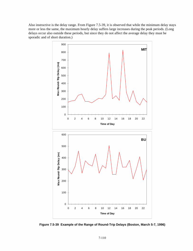
7-110
Also instructive is the delay range. From Figure 7.5-39, it is observed that while the minimum delay staysmore or less the same, the maximum hourly delay suffers large increases during the peak periods. (Longdelays occur also outside these periods, but since they do not affect the average delay they must besporadic and of short duration.)
MIT
0
100
200
300
400
500
600
700
800
900
0 2 4 6 8 10 12 14 16 18 20 22
T ime of Day
Ma
x Ro
und
-Trip
De
lay
(ms)
B U
0
100
200
300
400
500
600
0 2 4 6 8 10 12 14 16 18 20 22
T ime of Day
Ma
x Ro
und
-Trip
De
lay
(ms)
Figure 7.5-39 Example of the Range of Round-Trip Delays (Boston, March 5-7, 1996)

7-111
DIGIT AL
250
300
350
400
450
500
0 2 4 6 8 10 12 14 16 18 20 22
T ime of Day
Ma
x Ro
und
-Trip
De
lay
(ms)
CIT Y YE AR
0
200
400
600
800
1000
1200
1400
1600
0 2 4 6 8 10 12 14 16 18 20 22
T ime of Day
Ma
x Ro
und
-Trip
De
lay
(ms)
Figure 7.5-39 Example of the Range of Round-Trip Delays (Boston, March 5-7, 1996) (Cont’d)

7-112
7.5.2.4.3 Packet LossEqually important, from the point of view of information delivery, is packet loss. The co-operativeworkings of the Internet subject each packet to the perspective of being dropped at each router if the loadexceeds the queues or the processing capabilities of the router (many are not dedicated routers).
During the same period March 5-7, 1996, information was collected on packet loss for the sameorganizations as above. The samples are shown in Figure 7.5-40. The conclusion is that the packet losspeaks in general with the round-trip delay.
The higher loads in the network imply higher loads in the routers, more difficult routing, and more likelyoverload of the routers. When overloaded, the routers implement a non-discriminating rejection ofincoming packets to keep their load within reason, and not overflow.
MIT
0.0%
0.5%
1.0%
1.5%
2.0%
2.5%
0 2 4 6 8 10 12 14 16 18 20 22
T ime of Day
Min
-Av-
Ma
x Pa
cke
t Lo
ss
Figure 7.5-40 Minimum-Average-Maximum Packet Loss (Boston, March 5-7, 1996)

7-113
City Year
0.0%
0.1%
0.1%
0.2%
0.2%
0.3%
0.3%
0.4%
0.4%
0.5%
0 2 4 6 8 10 12 14 16 18 20 22
T ime of Day
Min
-Av-
Ma
x Pa
cke
t Lo
ss
Figure 7.5-40 Minimum-Average-Maximum Packet Loss (Boston, March 5-7, 1996) (Cont’d)
7.5.2.4.4 ConclusionsBesides the privacy and security issues of communicating over the Internet, which are still far fromresolved, the stochastic nature of the traffic on the Internet must be considered. The variance of theround-trip delay, as well as its average and the percentage of packet loss vary significantly over time.Thus, all those ITS applications requiring timely, consistent delivery of information should not use theInternet as a means of transferring information.
The occurrence of packet losses points also to the need of using a guaranteed delivery protocol like TCP,and restrict the use of non-guaranteed delivery protocols (like UDP) to non-essential, mostly repetitivetransactions (e.g., vehicle location,and normal, i.e., non-emergency, vehicle status reports).

7-114
7.6 Technology Survey and Assessment Summary
Section 7.5 presented a very broad survey and assessment of the telecommunications technologiesapplicable to the ITS Architecture. The key differentiating features of these technologies are summarizedin this section, as a quick reference for the convenience fo the reader. Table 7.6-1 provides an easy toread compilation of the terms and definitions used in the summary (and earlier in Section 7.5). Table 7.6-2 provides the summary comparison for terrestrial wireless data systems. Table 7.6-3 provides thesummary comparison for satellite systems. A fraction of the table entries contain a “?” indicating theunavailability of information at the time of writing this proprietary information. It should be kept in mindthat advanced technology evolves rapidly, so the information in the tables will need to be kept up to datein the future.
Table 7.6-1 Definition of the Entries in the Summary Tables
TERM DESCRIPTIONSATELLITE SYSTEMS Name of the satellite systemPARTNERSHIP List of the companies, organizations, or individuals who are
the principals and/or contributors of capitalSPECIFIC CHARACTERISTICSORBIT CLASS Classification of the satellite orbit
LEO - Low Earth Orbit. Altitude is typically below 10,000km.Big LEO - The term "Big" refers to the fact that the systemis designed for voice and data services. The operatingfrequency is above 1 GHz.Little LEO - Little LEO’s operate below 1 GHz, typically inthe VHF band. Designed for data services only.GEO - Geosynchronous Earth Orbit. Altitude isapproximately 36,000 km. Geostationary satellites havingthis orbit remain stationary over the same earth location.HEO - Highly Elliptical Orbit. Orbit has large eccentricity(continuously changing altitude)MEO - Medium Earth Orbit. Altitudes ranging from 3,000km to 20,000 km.ICO - Intermediate Circular Orbit, as termed by theEuropean satellite community. Same as MEO.
ALTITUDE (km) Orbital altitude in kilometers over the surface of the earth.NUMBER OF SATELLITES Total number of satellites in the specified satellite system.NUMBER OF PLANES Number of planes used in the satellite systemORBITAL PERIOD (minutes) Orbital period in minutesAVERAGE SATELLITE VISIBILITY TIME (minutes) Average time that a satellite is visible to the user’s
communication equipment on earth in minutes.MULTIPLE SATELLITE VISIBILITY yes - indicates that more than one satellite is visible to the
user’s communication equipment on earth.no - indicates that only one satellites is visible to the user’scommunication equipment on earth.
SATELLITE DIVERSITY yes - indicates that signals (carrying identical information)from two or more satellites are combined using a techniqueso as to improve reception for the land user.no - indicates that satellite diversity is not used.
MULTIPLE ACCESS TECHNIQUE Schemes used to provide multiple users access to thenetwork in order to minimize transmission overhead andmaximize overall throuput.Fixed-assignment channel-access :CDMA - Code Division Multiple Access.DS-SS - Direct Sequence Spread SpectrumFDMA - Frequency Division Multiple Access.FH-SS - Frequency Hopped Spread SpectrumSDMA - Spacial Division Multiple Access.

7-115
TERM DESCRIPTIONTDMA - Time Division Multiple Access.TDD - Time Division Duplexing (a form of TDMA)Multiplexing technique:FDM - Frequency Division MultiplexingTDM - Time Division MultiplexingRandom-Access Methods :Dynamic Slotted ALOHA protocolDSMA/CD - Digital Sense Multiple Access/ CollisionDetectionData Sense Multiple Access
MODULATION BPSK or PSK - Binary Phase Shift KeyingQFSK or 4-ary FSK- Frequency Shift Keying with fourorthogonal signalsGMSK - Gaussian Filtered Minimum Shift KeyingQPSK - Quadrature Phase Shift KeyingO-QPSK - Offset Quadrature Phase Shift Keying
FREQUENCY BAND VHF - Very High Frequency, 30 to 300 MHzUHF - Ultra High Frequency, 300 to 3000 MHzSHF - Super High Frequency, 3 to 30 GHzL-band - 390 MHz to 1.55 GHzS-band - 1.55 GHz to 5.2 GHzKa-band - 33 GHz to 36 GHzSMR band - 896-901 MHz, 935- 940 MHzCellular band - 824-849 MHz, 869-894 MHzISM - 902-928 MHzNarrowband PCS – 901 to 902 Mhz, 930 to 931MHz, 940-to 941MHzPaging - 929-932 MHz
UPLINK FREQUENCY BAND Allocated frequency band for transmission use from theearth user to the satellite.
DOWNLINK FREQ. BAND Allocated frequency band for transmission use from thesatellite to the earth user
DELAY CHARACTERISTICSMinimum mobile link one-way propagation time (ms) Minimum one-way propagation time between mobile user
and satellite in milliseconds.Maximum mobile link one-way propagation time (ms) Maximum one-way propagation time between mobile user
and satellite in milliseconds.SATELLITE ON-BOARD PROCESSING no - indicates a “bent-pipe” or transparent transponder
yes - indicates on-board signal regeneration beforeretransmission
HAND-OFF no - indicates that a terminal’s call within one cell area orsatellite can not be handed off to another cell or satellite asthe terminal moves into this new area.yes - indicates that a terminal’s call can be handed off to anadjacent cell or satellite
VOICE CIRCUITS PER SATELLITE Number of voice channels that a satellite canaccommodate
COVERAGE Geographic region in which service is provided by thesystem
MATURITY/ FEASIBILITYSCHEDULED OPERATION Estimated date of initial service of systemPERCENTAGE OF OBTAINED FINANCE Estimated percentage of obtained finance for the systemFCC LICENSE Date indicates the estimation of when the system obtained
an FCC license.CAPABILITIESVOICE RATE (kbps) Bit rate of digitized voice in kilobits per second.DATA RATE(kbps) Bit rate of data information. Units given in kilobits per
second.MOBILITYDUAL-MODE versus SINGLE MODE USER TERMINALS(land and satellite)
Dual - indicates that the terminal provides operating modesfor both satellite and terrestrial communications.Single - indicates that the terminal provides only oneoperating mode.
HAND-HELD versus PORTABLE USER TERMINALS Portable - indicates that the user terminal is a briefcase- orbag-sized self-contained unit combining antenna, battery,

7-116
TERM DESCRIPTIONtransceiver and handset.Hand-Held - indicates that the user terminal is sized to ahuman’s palm.
SYSTEM SECURITY Confidential Service - a service for which the content ofthe user’s data, traffic volumes and identities is keptconfidential or private. This service prevents unwarrantedextraction of information from the communication channel.Authentication Service - a service which ensures that thecontent of the user’s data and any other information isgenuine, unaltered, and complete. This service alsoensures that the information is not an unlawful replay ofinformation. This service prevents someone from injectingfalse data into the communication channel.Encryption - security mechanism which converts plaintextinto cyphertext. Cyphertext is unintelligible except to thoseindividuals/systems that know the secret of the decryptionalgorithm. An encryption service enables both confidentialand authentication services.
COSTSSYSTEM (Million US Dollars) Estimated cost of the full deployment of the system in
Millions of US Dollars.USER TERMINAL (US Dollars) Estimated cost of the terminal in US Dollars.VOICE RATE (US Dollars per minute) Estimated cost of voice service in US Dollars per minute.DATA RATE (US Dollars per kbyte) Estimated cost of data service in US Dollars per kilobyte.SERVICES List of services made available by the system.TARGETED APPLICATIONS Applications for which the system was designed.

7-117
Table 7.6-2 Summary Comparison of Wireless MAN and Cell-based Land Mobile Systems
RAM MobileData USA
ARDIS GEOTEK CDPD "CDPDng" SKYTEL METRICOMTAL
PARTNERSHIPS RAMBroadcastingCorporation,BellSouth(originallydeveloped byEricsson andSwedishTelecom)
Motorola andIBM
Geotek CDPD Forum(150companiesincludingcellularserviceproviders,equipmentmanufacturers,softwaredevelopers)
CDMA DataGroup
Mobile Tele-communicationsTechnology,Inc.
Metricom TetherlessAccess LTD.
SystemCharacteristics
COMMUNICATIONTECHNOLOGY
SMR SMR ESMR Cellular Cellular 2-way pagingMAN ?
SWITCHING packet packet packet packet andcircuit
packet andcircuit
n/a packet
OPEN STANDARD*Althoughpromoted as anopen architectureand a defactostandard, usesproprietarynetwork layerprotocol calledMPAK.
proprietary proprietary yes yes proprietary(Motorola'sReFLEX 500protocol)
proprietary proprietary?
RADIO CHANNELACCESSTECHNIQUE
proprietary,TDMA
proprietary,FDMA
proprietary,FHSS
Open,FDMA(packet radiooverlay onAMPS)
will be open,(packet radiooverlay onCDMA)
proprietary proprietary,FHSS
proprietary,CDMA?
MULTI-USERACCESSTECHNIQUE
Data SenseMultiple Access
Dynamic-SlottedALOHA
? Broadcastin Forwarddirection;Digital-SenseMultipleAccess/Collision Detection(DSMA/CM)in Reversedirection(packet radiooverlay onAMPS)
CDMA-SS ? ? ?
MODULATION GMSK 4-ary FSK ? GMSK ? BPSK/QPSKwide?
?
BANDWIDTH 12.5 kHz 25 kHz ? 30 kHz ? 25 kHz wide?
?
FREQUENCYBAND
SMR SMR ESMR Cellular Cellular NarrrowbandPCS
ISM ?
LICENSEDSPECTRUM
yes yes yes yes yes yes no no
NETWORKARCHITECTURE
macro cellular macro cellularmacrocellular
cellular cellular macrocellular
micro cellularwith nohandoffs,multihop
micro cellular,multihop
MOBILITY vehicle speeds vehicle speeds?? highwayspeeds
highwayspeeds
low vehiclespeeds
pedestrianspeeds
pedestrianspeeds
SYSTEMSECURITY
no (user providedencryption)
no (userprovidedencryption)
Medium (useof spreadspectrum)
high(encryptionalgorithms)
high(encryptionalgorithms)
no (userprovidedencryption)
Medium (useof spreadspectrum)
??
MATURITY OFSYSTEM
mature mature new mature future new new ?
SERVICESIP TRANSPORT no no future yes yes n/a yes yesIP TRANSPARENT(use of gateways)
yes yes future yes yes n/a no ?

7-118
Table 7.6-3 Summary Comparison of Proposed Satellite Systems
SATELLITESYSTEMS
ORBCOMM STARSYS VITASAT CONSTELLATION(formerly ARIES)
GLOBALSTAR IRIDIUM TELEDESIC ELLIPSO ICO (formerlyInmarsat-P)
ODYSSEY INMARSAT(A,B,C,M)
MSAT SKYCELL
PARTNERSHIP Orbital SciencesCorp.,Teleglobe,TRW
North AmericaCollection andLocation bySatellite(NACLS),ST System
Volunteers InTechnicalAssistance(VITA,VITACOMM)
ConstellationCommunication
Joint venture withTELEBRAS for theequatorial plane(ECCO)
Loral,Qualcomm
Motorola Bill Gates ofMicrosoft, andCraig McCawfounder ofMcCaw CellularCommunications,Inc. and chairmanof Teledesic
Ellipso MultipleGovernmentAgencies,Hughes
Teleglobe,TRW
MultipleGovernmentAgencies(InternationalMaritimeSatelliteOrganization,consortium of60 countries)
AmericanMobileSatellite Corp.,Glentel, Inc.,BCE,SparAerospace,Hughes,Mitsubishi,Westinghouse
AmericanMobileSatelliteCorp.(Hughes,AT&T,MTel,SingaporeTelecom
SpecificCharacteristicsORBIT CLASS Little LEO Little LEO Little LEO Big LEO Big LEO Big LEO Big LEO MEO and HEO MEO
(IntermediateCircular Orbits,ICO)
MEO GEO GEO GEO
ALTITUDE (km) 775, 950-1150depending onreference
1288 800 1018 1400 780 695-705 MEO is 8040;HEO is7846x520
10355 10354 35786 35786 35786
NUMBER OFSATELLITES
20, 26, 36depending onreference
24 2 to 3 48 48 plus 8 spare 66 plus 6 spare 840 plus up to 84spare
MEO is 6;HEO is 10
10 plus 3 spare 12 plus 3spare
Inmarsat phase2 uses 4satellites (since1992)Inmarsat phase3 uses 5satellites(projected 1996)
2 ?
NUMBER OFPLANES
3 ? ? 4 8 6 21 2 2 3 ? ? ?
ORBITAL PERIOD(minutes)
104.1-108.3 ? ? 105 114 100 99 MEO is 280;HEO is 180
359 360 N/A N/A N/A
AVERAGESATELLITEVISIBILITY TIME(minutes)
95% of time ? ? ? 8.21 5.54 1.74 ? 57.8 47.27 always always always
DUAL SATELLITEVISIBILITY
? ? ? ? 3 or more at poles >= 2 most of thetime
>= 2 North of40° South
usually >= 2 >= 2 ? ? ?
SATELLITEDIVERSITY
? ? ? ? yes no no yes yes no ? ? ?
MULTIPLEACCESSTECHNIQUE
? ? ? CDMA CDMA FDMA/ TDMA/TDD
TDMA, SDMA,FDMA, AdvancedTDMA
CDMA TDMA CDMA mostly FDMA TDMA/TDD FDMA
MODULATION PSK ? ? ? QPSK QPSK ? O-QPSK QPSK QPSK ? ? ?
UPLINKFREQUENCYBAND
VHF ? ? L-band L-band L-band Ka-band L-band S-band L-band ? L-band L-band
DOWNLINK FREQ.BAND
VHF ? ? S-band S-band L-band Ka-band S-band S-band S-band ? L-band L-band
DelayCharacteristics
Minimum mobilelink one-way
? ? ? 3.39 4.63 2.6 2.32 ? 34.5 34.6 238 238 238

7-119
Table 7.6-3 Summary Comparison of Proposed Satellite Systems
SATELLITESYSTEMS
ORBCOMM STARSYS VITASAT CONSTELLATION(formerly ARIES)
GLOBALSTAR IRIDIUM TELEDESIC ELLIPSO ICO (formerlyInmarsat-P)
ODYSSEY INMARSAT(A,B,C,M)
MSAT SKYCELL
propagation time(ms)
Maximum mobilelink one-way
propagation time(ms
5 sec ? ? ? 11.5 8.2 3.4 38.7 48 44.3 275 ? ?
SATELLITE ON-BOARDPROCESSING
? ? ? ? no yes yes ? ? no no no no
HAND-OFF ? ? ? ? yes yes yes yes, terminalnot involved
yes yes ? ? ?
VOICE CIRCUITSPER SATELLITE
? ? ? ? 2000-3000 1100 (powerlimited)
100,000 (16 kbpschannels)
? 4500 2300 ? ? ?
COVERAGE US now,Global future
Global Global,designed fordevelopingcountriesincluding SouthAmerica, Africa
Global within +/- 70°latitude
Global Global, except for2° hole at poles;95% of earth'ssurface
North of 50°South
Global major landmasses
Global North America,Hawaii,Caribbean
NorthAmerica
MATURITY/FEASIBILITYSCHEDULEDOPERATION
CurrentlyOperational inUS; 1996 Canadaand Mexico; 1997Europe and LatinAmerica
1996 1996 1998 1998 1998 2001 1998 2000 2000 Operationalsince 1993
1996 ?
PERCENTAGE OFFINANCEOBTAINED THUSFAR
~100% ? ? ~15% ~70% ~30% ? ? 58% ? ? ? ?
FCC LICENSE late 1994 ExperimentalLicense in 1992
? ? Jan. 1995 ? ? ? ? ? WARC ‘92 andWRC ‘95
? 1989
CAPABILITIES
VOICE RATE(kbps)
? ? ? 4.8 adaptive2.4/4.8/9.6
2.4/4.8 16 4.15 4.8 4.8 6.4 to 16depending onsystem
? ?
DATA RATE(kbps) 2.4 uplink, 4.8downlink
? ? 2.4 7.2 sustainedthroughput
2.4 16 to 2048 0.3 to 9.6 2.4 9.6 0.6, 2.4, 9.6, 64depending onsystem
2.4 1.2-4.8
MOBILITY ? ? ? ? ? ? Fixed ? ? ? Fixed andMobile
Fixed (Canadaand Alaska);Mobile(Contiguous48 States)
Full mobility(vehicles,ships, andairplanes)
DUAL-MODE vs.SINGLE MODEUSER TERMINALS(land and satellite)
? ? ? ? DUAL DUAL SINGLE DUAL DUAL DUAL DUAL (driversfor ARDIS,CDPD, GSM)
DUAL ?
HAND-HELD vs.PORTABLE USERTERMINALS
Portable andHand-held
? Portable Hand-held Hand-held Hand-held Portable Hand-held Hand-held Hand-held Portable Portable Portable

7-120
Table 7.6-3 Summary Comparison of Proposed Satellite Systems
SATELLITESYSTEMS
ORBCOMM STARSYS VITASAT CONSTELLATION(formerly ARIES)
GLOBALSTAR IRIDIUM TELEDESIC ELLIPSO ICO (formerlyInmarsat-P)
ODYSSEY INMARSAT(A,B,C,M)
MSAT SKYCELL
SYSTEMSECURITY
? ? ? ? ? ? encryption ? ? ? ? ? authenti-cation only
COSTS
SYSTEM (MillionU.S. Dollars)
? ? ? $1,700 $2,000 $3,700 $9,000 $750 $2,600 $1,800 ? ? ?
USER TERMINAL $100 -$400 ? $3500 ? ~$750/terminal;$1000-$1200 fortelephone
$2500-$3000 ? ~$1000; $300add-on todigital cellularunit
"SeveralHundred"
~$300 $5000-$35,000depending onsystem
$5000-$6000 ?
VOICE RATE (USDollars per minute)
? ? ? ? $0.35-$0.55 $3.00 ? $0.50 $1-$2 $0.75 ; $24monthlycharge
$2.00-$8.00depending onsystem
$2.50 Standard,$25/month,$1.49/minuteBusiness,$175/month,200 minutesfree,$0.85/minutevoice, data,fax
DATA RATE (USDollars per kbyte)
$1.00 per 100bytes
? $50/month forup to 100 kbytes
? ? ? ? ? ? ? $1.00-$1.50 ? similar tovoice servicecosts
SERVICES two-waymessaging,RDSS
one-way data,two-waymessaging
two-waymessaging;store andforward withtypically 90minute messagedelay and asmuch as 12hour delay.
voice, data, fax Voice, data, fax,paging, shortmessageservice, RDSS
Voice, data, fax,paging,messaging,RDSS
Voice, data, fax,paging, video
Voice, data,fax, paging,messaging,RDSS
Voice, data, fax,paging
Voice, data,fax, paging,messaging,radiodeterminationsatelliteservices(RDSS)
voice, data, fax,e-mail, store-and-forward,alerting, positiondetermination
voice, data,fax, dispatchradio
Voice, data,fax, locationdetermina-tion
TARGETEDAPPLICATIONS
emergencycomm., 2 way-mail, remoteresourcemonitoring
emergencycomm. stolenasset recovery,hazardousmaterial tracking
Store-and-forward data
extension of thecellular network
worldwidecommunication
worldwidecommunication
ISDN to ruralbusinesses andremote terminals(fixed)
extension ofcellularnetwork
global phonethroughintegration withcellular services
extension ofcellularnetwork
worldwidecommunication
mobile office,positiondetermination,e-mail,monitoring,voicedispatching (2-way),broadcast andmulticastmessaging
transporta-tion,maritime,aeronauticalremote siteindustries

8-1
8. COMMUNICATION SYSTEMS PERFORMANCE – A CASE STUDY
This section presents an important thrust in the ITS Architecture development effort. The use of existing(i.e., commercially available) and emerging telecommunication infrastructures is integral to the ITSArchitecture and corner stone to its feasibility. In this section detailed, in-depth analyses and simulationsare performed to support this architecture development philosophy. Through the results of thesimulations in a specific case study, it will be demonstrated that the ITS data loads, particularly for widearea communications, can be handled by existing, i.e., commercially deployed and available systems.
For wide area communications in particular, the ITS Architecture leverages the communicationinfrastructures put in place by the very broad telecommunication industry (see Sections 3 and 7 for thetechnologies applicable to the myriad ITS data flows). Correspondingly, the evaluation strategy in thissection utilizes the expertise that has been developed in the telecommunications industry in planning,deploying and operating these infrastructures. More specifically, the evaluation uses and builds uponsimulation tools that have been developed for real systems, i.e., which have been and continue to bedeployed commercially. The simulation tools and various of their results have been validated over timeby a cross-section of leading industry partners. These partners include GTE, AT&T/McCaw, BellAtlantic, NYNEX, and others in the CDPD Forum for Cellular Digital Packet Data (CDPD), andQualcomm, GTE, Nokia, and others in the CDMA Development Group (CDG) for CDMA. In addition tothe established tools, the use of existing and emerging standards (e.g., CDPD in wireless communication)simplifies the evaluation process through a structured, well accepted, and reliable definition of the keysimulation parameters. This, in turn, aids the Independent Verification and Validation (IV&V) processsought by the Government.
The ITS communication systems simulation is configured into two segments – wireless and wireline –reflecting the nature of the modern communication infrastructure. Although the wireless segmenttypically limits performance, the performance of both segments is required for a complete and thoroughcharacterization of the communication layer of the ITS system architecture.
Significant resources were dedicated to analyzing, simulating, and evaluating a specific wirelessinfrastructure that can accommodate the wide area ITS services. For practical reasons, the wirelesssimulation effort had to be constrained to open, already standardized systems. Thus, given that CellularDigital Packet Data (CDPD) is the only fully standardized, open-system for data communications overcellular (in the U.S. or abroad), with the advantage of being in an advanced deployment stage, CDPD isused as a case study to show the feasibility of a wide-area ITS cellular solution. This does not imply,however, any a priori commitment to CDPD as the ITS wide-area delivery platform. Rather, it serves todemonstrate the feasibility of the architecture in that commercially available wireless systems do indeedexist that can handle the ITS data load requirements into the foreseeable future.
Meanwhile, wireline simulation is not neglected, it is used to aid in designing a candidate backbonenetwork to provide connectivity and access to the wireless assets and to tie together the fixedtransportation entities.
End-to-end communication system performance will be obtained by integrating the simulation efforts inthese two areas. Performance results for the overall communication system associated with given usersand/or user services will be obtained. Naturally, the end-to-end communication system performance

8-2
should be tied to the corresponding latencies identified in the Mission Definition document for the ITSservices (whose offering involves both communication and transportation subsystems). The selection ofthe best communication architecture and technologies can then be pursued to meet the broad objectivesof sufficiency, cost effectiveness, and risk mitigation through proper utilization of existing and emergingwireless and wireline technologies.
With the objective of promoting user acceptance for each medium, and especially for those that involveair-time charges (e.g., wireless data systems like CDPD), care is taken to utilize a message structure thatminimizes user cost by reducing overhead (transmitting the required information, and not requiringunnecessary padding to fit fixed message sizes). Simultaneously, but secondarily, this approach optimizessystem performance by increasing throughput for a given infrastructure, or improving performance forthe same effective user load.
8.1 Wireless Systems Performance
The objective of this section is to determine whether the communications element or "layer" of thesystem architecture is both sufficient and efficient at all stages of deployment, especially for the 1997,2002, and 2012 time frames.
The analysis of the 2012 time frame was performed at earlier stages of the National ITS ArchitectureStudy (Phase I), and is reported herein, even though the loads date back to the Phase II IPR2 submission(Logical and Physical Architecture data flows of August 1995). The objective of presenting these resultsis to show system performance with the highest ITS only loads anticipated for that time frame.
The 2002 time frame was selected for complete evaluation upon discussions with the Government andthe Technical Review Team. We will analyze the performance of the CDPD system for the cases of ITSonly, ITS plus Non-ITS, and ITS plus Non-ITS in case of Incident. These simulations will use worst caseloads for the most recent (January 1996) Logical and Physical Architecture data flows.
8.1.1 Scope of Performance Analysis
The peak period scenario to be analyzed is obtained from the actual cellular deployment for eachGovernment chosen scenario (which we assume not to expand with time thereby implying worst caseperformance results). The peak voice load was computed for each sector from the Erlang-B formula for2% blocking probability. For the ITS data load, proportionality to the voice load (i.e., to the number ofcellular users) was assumed. The underlying implication is that there is a proportionality between thenumber of cellular voice users and the number of ITS users (i.e., the concept of a “wireless” use patternis assumed for the lack of better information). Thus, the overall ITS data load was divided proportionallyby the sectors as a function of their voice load.
CDPD performance was simulated for two of the three scenarios defined by the Government, namelyUrbansville, and Thruville. Mountainville was analyzed from the point of view of cellular coverage, butCDPD was not exercised because it is very unlikely that CDPD will be deployed in Lincoln County, MTat that time, given the small population density, and the foreseeable loads. That, however, does not meanthat users in those regions would be left out of data coverage. Indeed, through Circuit-Switched CDPD,everyone could piggyback on that infrastructure to exchange data wherever cellular coverage reaches.
8.1.1.1 Urbansville 2002 and 2012
In Phase I, we analyzed the case of one reserved CDPD channel plus another one dynamically assignedas a function of availability and demand. In Phase II, we considered the case of one reserved CDPD

8-3
channel without any additional dynamically assigned channels, as well as a totally dynamic solution forthe CDPD problem, with no reserved channels.
8.1.1.1.1 Cellular Deployment in the Detroit MSA
The CDPD deployment under consideration will be analyzed as an overlay onto the real cellularinfrastructure deployed in the Detroit area (up-to-date as of November 1993). The definition of thisrealistic deployment required the compilation of a very large set of detailed infrastructure parametersfrom the FCC filings of the Detroit Cellular Telephone Company (DCTC).
The DCTC FCC filing information is summarized in Table 8.1-1. An example of base station (BS)characterization thus obtained is provided in Table 8.1-2 for DCTC Site #25. Each antenna wascharacterized based, whenever possible, on manufacturer provided information, and otherwise by readingfrom polar plots filed with the site authorization requests. An example is shown in Table 8.1-3.
The area analyzed in this case study corresponds to the total area of the three counties that make upUrbansville. In Figure 8.1-1, we schematically present the distribution of the BSs read from the FCCfilings. Note that it was not possible to include the boundaries of Urbansville since they were notprovided by the Government to the Teams. Figure 8.1-2 (obtained using GRANET) presents the bestserver map for the three counties encompassing Urbansville (in the Detroit area). The ragged boundariesof the cells reflect actual propagation conditions, thus showing how topography, topology, and land useaffect conditions.
In this realistic test case, the uniformity assumption that had been used early in Phase I has been removed(the number of channels in a given sector varies from 8 to 37). The peak voice was computed for eachsector from the Erlang-B formula for 2% blocking probability. For the IVHS data load, the sameassumption was made of proportionality to the voice load (i.e., to the number of cellular users). Thus, theoverall Urbansville IVHS data load was divided proportionally by the sectors.

8-4
Table 8.1-1 Summary of DCTC FCC Filings (Nov. 1993)
DCTCLocationNumber
Location Code Name NLatitude
WLongitude
SectorNumber
Numberof
Channels
Antenna Type ERP (W)
3 Proud Lake 42-33-40 83-34-20 1 16 DB874H83 100
3 Proud Lake 42-33-40 83-34-20 2 24 DB874H83 20
3 Proud Lake 42-33-40 83-34-20 3 15 DB874H83 100
4 Novi 42-28-47 83-27-40 1 20 ALP8013-N 35
4 Novi 42-28-47 83-27-40 2 28 ALP8013-N 36
4 Novi 42-28-47 83-27-40 3 31 ALP8013-N 50
7 Mt. Clemens 42-32-26 82-53-25 1 20 ALP8013-N 75
7 Mt. Clemens 42-32-26 82-53-25 2 16 ALP8013-N 25
7 Mt. Clemens 42-32-26 82-53-25 3 31 ALP8013-N 27
8 Anchorville 42-45-25 82-44-25 1 12 ALP11011-N 86
8 Anchorville 42-45-25 82-44-25 2 19 ALP11011-N 60
8 Anchorville 42-45-25 82-44-25 3 12 ALP11011-N 89
9 Holly 42-47-02 83-32-05 1 16 PD-1136 83.2
9 Holly 42-47-02 83-32-05 2 15 PD-1136 83.2
12 WDIV Tower 42-28-58 83-12-19 1 16 ALP8010 12.5
12 WDIV Tower 42-28-58 83-12-19 2 24 ALP8010 50
12 WDIV Tower 42-28-58 83-12-19 3 24 ALP8010 50
14 Lake Angelous 42-41-25 83-17-50 1 24 DB-564 75
14 Lake Angelous 42-41-25 83-17-50 2 16 ALP8013-N 25
14 Lake Angelous 42-41-25 83-17-50 3 20 ALP8013-N 50
15 Rochester 42-40-42 83-07-27 1 24 DB-564 75
15 Rochester 42-40-42 83-07-27 2 22 DB-834 40
15 Rochester 42-40-42 83-07-27 3 28 DB874H83 75
16 Livonia 42-19-35 83-25-42 1 16 ALP8010 50
16 Livonia 42-19-35 83-25-42 2 19 ALP8010 75
16 Livonia 42-19-35 83-25-42 3 35 DB874H83 50
17 Walled Lake 42-34-09 83-26-30 1 20 DB874H83 50
17 Walled Lake 42-34-09 83-26-30 2 16 DB874H83 25
17 Walled Lake 42-34-09 83-26-30 3 19 DB874H83 50
18 Warren 42-36-27 83-02-33 1 28 DB874H83 100
18 Warren 42-36-27 83-02-33 2 24 DB874H83 50
18 Warren 42-36-27 83-02-33 3 19 DB874H83 25
19 Dearborn 42-18-52 83-09-07 1 16 ALP8013-N 73
19 Dearborn 42-18-52 83-09-07 2 24 DB882H60 64
19 Dearborn 42-18-52 83-09-07 3 27 DB874H83 64
21 Bloomfield Hills 42-36-32 83-17-35 1 20 DB872H83 25
21 Bloomfield Hills 42-36-32 83-17-35 2 28 ALP8013-N 30
21 Bloomfield Hills 42-36-32 83-17-35 3 26 DB874H83 25
22 Franklin 42-30-07 83-18-33 1 20 ALP8013-N 10
22 Franklin 42-30-07 83-18-33 2 32 ALP8013-N 6

8-5
22 Franklin 42-30-07 83-18-33 3 36 ALP8013-N 27
23 Redford 42-24-07 83-16-29 1 16 DB882H60 25
23 Redford 42-24-07 83-16-29 2 20 DB872H83 43
23 Redford 42-24-07 83-16-29 3 20 ALP8013-N 50
24 Strohs 42-20-12 83-01-03 1 20 DB883H60 75
24 Strohs 42-20-12 83-01-03 2 16 PD-1132 50
25 Detroit West 42-23-13 83-10-50 1 16 ALP8010-N 57
25 Detroit West 42-23-13 83-10-50 2 16 ALP8010-N 50
25 Detroit West 42-23-13 83-10-50 3 23 ALP8010-N 30
26 Detroit Baltimore 42-22-13 83-04-06 1 24 DB872H83 20
26 Detroit Baltimore 42-22-13 83-04-06 2 24 DB882H60 20
26 Detroit Baltimore 42-22-13 83-04-06 3 23 DB872H83 18
27 Grosse Pointe 42-24-11 82-58-08 1 20 ALP8010 50
27 Grosse Pointe 42-24-11 82-58-08 2 16 ALP8010 50
27 Grosse Pointe 42-24-11 82-58-08 3 19 ALP8010 50
28 Dearborn West 42-19-51 83-13-13 1 16 DB-834 100
28 Dearborn West 42-19-51 83-13-13 2 16 DB-834 100
28 Dearborn West 42-19-51 83-13-13 3 15 DB-834 100
29 East Detroit 42-29-28 83-02-32 1 16 DB-564S 100
29 East Detroit 42-29-28 83-02-32 2 16 DB-564S 100
29 East Detroit 42-29-28 83-02-32 3 15 DB-564S 100
30 Clawson 42-32-29 83-07-58 1 24 DB874H83 50
30 Clawson 42-32-29 83-07-58 2 24 DB874H83 50
30 Clawson 42-32-29 83-07-58 3 20 DB874H83 50
31 Bloomfield Hills 42-32-26 83-17-03 1 18 DB-834 100
31 Bloomfield Hills 42-32-26 83-17-03 2 15 DB-834 66
31 Bloomfield Hills 42-32-26 83-17-03 3 12 DB-834 66
32 Inkster 42-17-43 83-17-42 1 24 ALP8013-N 12.5
32 Inkster 42-17-43 83-17-42 2 24 ALP8013-N 50
32 Inkster 42-17-43 83-17-42 3 16 ALP8013-N 50
33 Hazel Park 42-27-55 83-05-01 1 16 DB-834 100
33 Hazel Park 42-27-55 83-05-01 2 16 DB-834 100
33 Hazel Park 42-27-55 83-05-01 3 16 DB-834 100
34 Pleasant Ridge 42-28-53 83-08-22 1 16 DB-834 50
34 Pleasant Ridge 42-28-53 83-08-22 2 24 DB874H83 50
34 Pleasant Ridge 42-28-53 83-08-22 3 23 ALP8007-N 12.5
35 Birmingham 42-32-43 83-11-37 1 24 ALP8010 50
35 Birmingham 42-32-43 83-11-37 2 16 ALP8010 25
35 Birmingham 42-32-43 83-11-37 3 19 ALP8010 50
36 Northville 42-23-50 83-26-11 1 20 ALP8010-N 35
36 Northville 42-23-50 83-26-11 2 24 ALP8010-N 67
36 Northville 42-23-50 83-26-11 3 16 ALP8013-N 100
37 Farmington Hills 42-29-52 83-22-45 1 12 LPD-7907 58
37 Farmington Hills 42-29-52 83-22-45 2 16 LPD-7907 58
37 Farmington Hills 42-29-52 83-22-45 3 13 LPD-7907 58
38 Auburn Hills 42-38-03 83-12-58 1 14 DB874H83 100

8-6
38 Auburn Hills 42-38-03 83-12-58 2 12 DB874H83 50
38 Auburn Hills 42-38-03 83-12-58 3 19 DB874H83 75
39 Sterling Heights 42-33-01 83-00-03 1 14 DB-834 80
39 Sterling Heights 42-33-01 83-00-03 2 12 DB-834 80
39 Sterling Heights 42-33-01 83-00-03 3 16 DB-834 80
40 Southfield 42-27-00 83-16-57 1 16 DB-834 75
40 Southfield 42-27-00 83-16-57 2 16 DB-834 75
40 Southfield 42-27-00 83-16-57 3 15 DB-834 75
42 Detroit N. 42-27-18 83-00-28 1 16 DB-834 100
42 Detroit N. 42-27-18 83-00-28 2 16 DB-834 100
42 Detroit N. 42-27-18 83-00-28 3 16 DB-834 100
43 Big Beaver 42-34-35 83-07-37 1 16 DB-834 100
43 Big Beaver 42-34-35 83-07-37 2 16 DB-834 100
43 Big Beaver 42-34-35 83-07-37 3 16 DB-834 100
44 Highland Park 42-24-07 83-07-29 1 16 DB-834 100
44 Highland Park 42-24-07 83-07-29 2 16 DB-834 100
44 Highland Park 42-24-07 83-07-29 3 15 DB-834 100
45 Oak Park 42-26-20 83-11-41 1 16 DB-834 100
45 Oak Park 42-26-20 83-11-41 2 16 DB-834 100
45 Oak Park 42-26-20 83-11-41 3 15 DB-834 100
46 Taylor 42-13-34 83-14-08 1 16 DB-834 100
46 Taylor 42-13-34 83-14-08 2 16 DB-834 100
46 Taylor 42-13-34 83-14-08 3 16 DB-834 100
47 Farmington 42-26-26 83-21-52 1 20 DB-834 30
47 Farmington 42-26-26 83-21-52 2 11 DB874H83 50
47 Farmington 42-26-26 83-21-52 3 16 DB-834 63
48 East Livonia 42-22-24 83-22-13 1 20 ALP8010-N 67
48 East Livonia 42-22-24 83-22-13 2 16 ALP8013-N 30
48 East Livonia 42-22-24 83-22-13 3 14 ALP8013-N 13
49 Minnow Lake 42-34-44 83-16-54 1 19 ALP8013-N 100
49 Minnow Lake 42-34-44 83-16-54 2 16 ALP8013-N 50
49 Minnow Lake 42-34-44 83-16-54 3 16 ALP8013-N 100
50 Lathrup 42-29-12 83-16-10 1 20 ALP8010 80
50 Lathrup 42-29-12 83-16-10 2 20 ALP8010 40
50 Lathrup 42-29-12 83-16-10 3 15 ALP8010 25
51 Harper Woods 42-28-05 82-55-14 1 20 ALP8013-N 79
51 Harper Woods 42-28-05 82-55-14 2 20 ALP8010-N 30
51 Harper Woods 42-28-05 82-55-14 3 14 ALP8013-N 79
52 Orchard Lake 42-33-35 83-22-20 1 19 ALP8010-N 25
52 Orchard Lake 42-33-35 83-22-20 2 20 ALP8010-N 25
52 Orchard Lake 42-33-35 83-22-20 3 10 ALP8013-N 100
53 Troy 42-36-13 83-10-05 1 16 DB-834 100
53 Troy 42-36-13 83-10-05 2 16 DB-834 100
53 Troy 42-36-13 83-10-05 3 16 DB-834 100
54 Elizabeth Lake 42-38-21 83-22-52 1 16 DB-834 100
54 Elizabeth Lake 42-38-21 83-22-52 2 16 DB-834 100
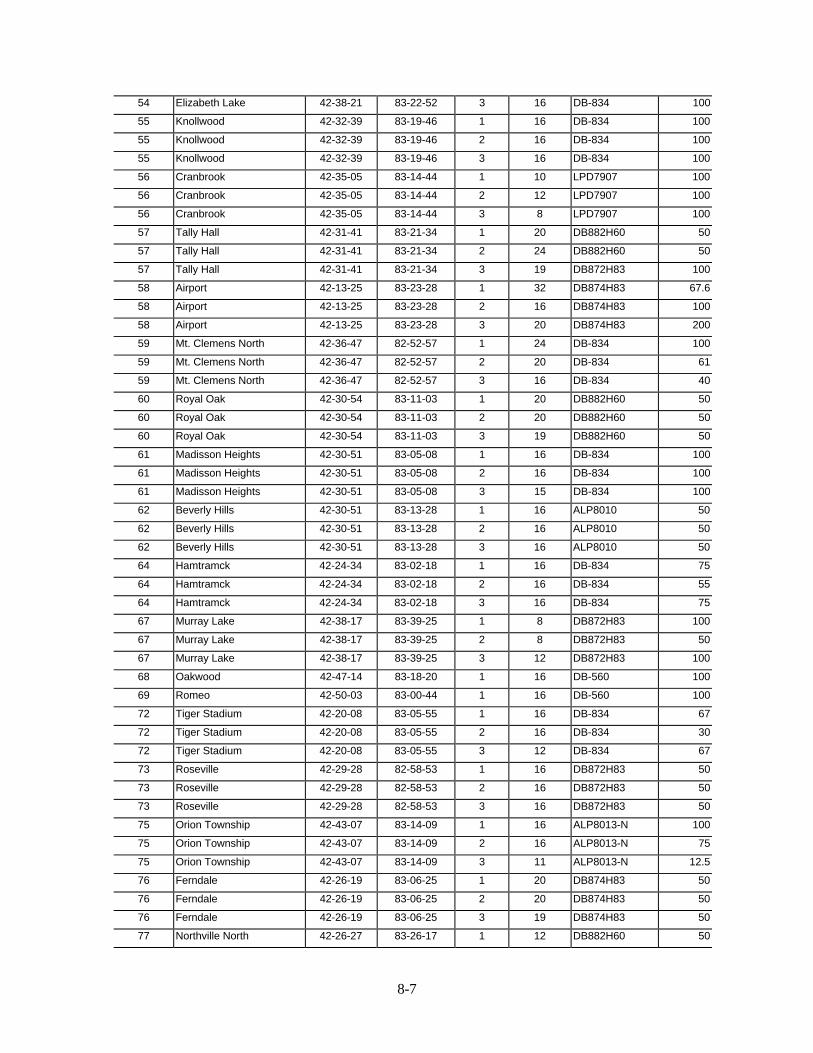
8-7
54 Elizabeth Lake 42-38-21 83-22-52 3 16 DB-834 100
55 Knollwood 42-32-39 83-19-46 1 16 DB-834 100
55 Knollwood 42-32-39 83-19-46 2 16 DB-834 100
55 Knollwood 42-32-39 83-19-46 3 16 DB-834 100
56 Cranbrook 42-35-05 83-14-44 1 10 LPD7907 100
56 Cranbrook 42-35-05 83-14-44 2 12 LPD7907 100
56 Cranbrook 42-35-05 83-14-44 3 8 LPD7907 100
57 Tally Hall 42-31-41 83-21-34 1 20 DB882H60 50
57 Tally Hall 42-31-41 83-21-34 2 24 DB882H60 50
57 Tally Hall 42-31-41 83-21-34 3 19 DB872H83 100
58 Airport 42-13-25 83-23-28 1 32 DB874H83 67.6
58 Airport 42-13-25 83-23-28 2 16 DB874H83 100
58 Airport 42-13-25 83-23-28 3 20 DB874H83 200
59 Mt. Clemens North 42-36-47 82-52-57 1 24 DB-834 100
59 Mt. Clemens North 42-36-47 82-52-57 2 20 DB-834 61
59 Mt. Clemens North 42-36-47 82-52-57 3 16 DB-834 40
60 Royal Oak 42-30-54 83-11-03 1 20 DB882H60 50
60 Royal Oak 42-30-54 83-11-03 2 20 DB882H60 50
60 Royal Oak 42-30-54 83-11-03 3 19 DB882H60 50
61 Madisson Heights 42-30-51 83-05-08 1 16 DB-834 100
61 Madisson Heights 42-30-51 83-05-08 2 16 DB-834 100
61 Madisson Heights 42-30-51 83-05-08 3 15 DB-834 100
62 Beverly Hills 42-30-51 83-13-28 1 16 ALP8010 50
62 Beverly Hills 42-30-51 83-13-28 2 16 ALP8010 50
62 Beverly Hills 42-30-51 83-13-28 3 16 ALP8010 50
64 Hamtramck 42-24-34 83-02-18 1 16 DB-834 75
64 Hamtramck 42-24-34 83-02-18 2 16 DB-834 55
64 Hamtramck 42-24-34 83-02-18 3 16 DB-834 75
67 Murray Lake 42-38-17 83-39-25 1 8 DB872H83 100
67 Murray Lake 42-38-17 83-39-25 2 8 DB872H83 50
67 Murray Lake 42-38-17 83-39-25 3 12 DB872H83 100
68 Oakwood 42-47-14 83-18-20 1 16 DB-560 100
69 Romeo 42-50-03 83-00-44 1 16 DB-560 100
72 Tiger Stadium 42-20-08 83-05-55 1 16 DB-834 67
72 Tiger Stadium 42-20-08 83-05-55 2 16 DB-834 30
72 Tiger Stadium 42-20-08 83-05-55 3 12 DB-834 67
73 Roseville 42-29-28 82-58-53 1 16 DB872H83 50
73 Roseville 42-29-28 82-58-53 2 16 DB872H83 50
73 Roseville 42-29-28 82-58-53 3 16 DB872H83 50
75 Orion Township 42-43-07 83-14-09 1 16 ALP8013-N 100
75 Orion Township 42-43-07 83-14-09 2 16 ALP8013-N 75
75 Orion Township 42-43-07 83-14-09 3 11 ALP8013-N 12.5
76 Ferndale 42-26-19 83-06-25 1 20 DB874H83 50
76 Ferndale 42-26-19 83-06-25 2 20 DB874H83 50
76 Ferndale 42-26-19 83-06-25 3 19 DB874H83 50
77 Northville North 42-26-27 83-26-17 1 12 DB882H60 50

8-8
77 Northville North 42-26-27 83-26-17 2 12 DB882H60 25
77 Northville North 42-26-27 83-26-17 3 8 DB872H83 100
79 Clarkston 42-43-54 83-22-28 1 16 DB874H83 100
79 Clarkston 42-43-54 83-22-28 2 16 DB874H83 100
79 Clarkston 42-43-54 83-22-28 3 16 DB874H83 100
83 Pontiac South 42-38-53 83-16-09 1 16 DB874H83 50
83 Pontiac South 42-38-53 83-16-09 2 16 DB874H83 50
83 Pontiac South 42-38-53 83-16-09 3 16 DB874H83 50
84 Downtown Detroit 42-19-37 83-02-44 1 16 DB882H60 50
84 Downtown Detroit 42-19-37 83-02-44 2 15 DB874H83 50
85 Mound 42-33-09 83-02-42 1 16 DB874H83 25
85 Mound 42-33-09 83-02-42 2 12 DB874H83 50
85 Mound 42-33-09 83-02-42 3 12 DB874H83 50
86 Canton 42-16-38 83-27-04 1 16 DB874H83 50
86 Canton 42-16-38 83-27-04 2 16 DB874H83 50
86 Canton 42-16-38 83-27-04 3 16 DB874H83 100
87 Detroit West II 42-24-07 83-13-13 1 12 DB874H83 50
87 Detroit West II 42-24-07 83-13-13 2 12 DB874H83 50
87 Detroit West II 42-24-07 83-13-13 3 12 DB874H83 50
89 Livonia Mall 42-24-49 83-20-11 1 12 DB874H83 50
89 Livonia Mall 42-24-49 83-20-11 2 12 DB874H83 50
89 Livonia Mall 42-24-49 83-20-11 3 12 DB874H83 50
90 Northwestern Hwy 42-27-56 83-14-00 1 16 DB874H83 14
90 Northwestern Hwy 42-27-56 83-14-00 2 16 DB874H83 50
90 Northwestern Hwy 42-27-56 83-14-00 3 16 DB874H83 25
92 Rochester South 42-39-26 83-09-19 1 12 ALP8013-N 50
92 Rochester South 42-39-26 83-09-19 2 12 ALP8013-N 50
92 Rochester South 42-39-26 83-09-19 3 12 ALP8013-N 50
94 Grosse Pointe Park 42-22-16 82-57-06 1 12 ALP4014-N 100
94 Grosse Pointe Park 42-22-16 82-57-06 2 12 ALP6011-N 50
95 Airport North 42-14-44 83-18-25 1 12 ALP8010 50
95 Airport North 42-14-44 83-18-25 2 12 ALP8010 50
95 Airport North 42-14-44 83-18-25 3 16 ALP8010 100
96 Dearborn Heights 42-20-59 83-16-32 1 16 DB874H83 50
96 Dearborn Heights 42-20-59 83-16-32 2 16 DB874H83 25
96 Dearborn Heights 42-20-59 83-16-32 3 16 DB874H83 50
99 Grosse Pointe Yacht Club 42-26-04 82-52-21 1 8 LPD-7907 5
99 Grosse Pointe Yacht Club 42-26-04 82-52-21 2 8 LPD-7907 100
114 White Lake 42-39-29 83-32-45 1 8 ALP8013-N 50
114 White Lake 42-39-29 83-32-45 2 8 ALP8013-N 50
114 White Lake 42-39-29 83-32-45 3 12 ALP8013-N 50
115 Keego Harbor 42-36-42 83-19-47 1 16 ALP8010 25
115 Keego Harbor 42-36-42 83-19-47 2 12 ALP8010 25
115 Keego Harbor 42-36-42 83-19-47 3 12 ALP8010 25
116 Garfield 42-36-22 82-57-04 1 16 ALP8010 100
116 Garfield 42-36-22 82-57-04 2 12 ALP8010 50

8-9
116 Garfield 42-36-22 82-57-04 3 16 ALP8010 50
120 Halstead 42-29-35 83-25-18 1 16 DB874H83 25
120 Halstead 42-29-35 83-25-18 2 16 DB874H83 25
120 Halstead 42-29-35 83-25-18 3 16 DB874H83 50
124 Stephenson Hwy 42-30-37 83-06-58 1 16 ALP8010 50
124 Stephenson Hwy 42-30-37 83-06-58 2 16 ALP8010 25
124 Stephenson Hwy 42-30-37 83-06-58 3 12 ALP8010 23.3
132 Troy South 42-33-47 83-09-03 1 16 DB874H83 25
132 Troy South 42-33-47 83-09-03 2 16 DB874H83 25
132 Troy South 42-33-47 83-09-03 3 16 DB874H83 25
133 Birmingham Downtown 42-32-44 83-12-51 1 20 DB872H83 100
133 Birmingham Downtown 42-32-44 83-12-51 2 20 DB872H83 50
133 Birmingham Downtown 42-32-44 83-12-51 3 20 DB872H83 50
150 Allen Park 42-16-19 83-12-04 1 16 DB874H83 25
150 Allen Park 42-16-19 83-12-04 2 16 DB874H83 50
150 Allen Park 42-16-19 83-12-04 3 16 DB874H83 25
155 Haggerty x 14 Mile Road 42-31-42 83-26-28 1 16 ALP8010 50
155 Haggerty x 14 Mile Road 42-31-42 83-26-28 2 16 ALP8010 50
155 Haggerty x 14 Mile Road 42-31-42 83-26-28 3 16 ALP8010 100
Table 8.1-2 Characterization of the DCTC Site #25
SITE_NAME Detroit WestSITE_ID DCTC-025LATITUDE 42 23 13 NLONGITUDE 83 10 50 EFREQUENCY 860 MHzVOICE_CHANNEL_DATANUMBER_OF_SECTORS 3FOR_SECTOR 1ANTENNA_HEIGHT 159 FTANTENNA_MODEL_NUMBER ALP8010-NANTENNA_MAIN_LOBE 30 degreesERP 57 WNUMBER_OF_CHANNELS 16CONTROL _CHANNEL 333VOICE_CHANNELS 270 250 228 207 186 165 144 123 102 81 60 39 18FOR_SECTOR 2ANTENNA_HEIGHT 159 FTANTENNA_MODEL_NUMBER ALP8010-NANTENNA_MAIN_LOBE 150 degreesERP 50 WNUMBER_OF_CHANNELS 16CONTROL _CHANNEL 321VOICE_CHANNELS 258 237 216 195 174 153 132 111 90 69 48 27 6FOR_SECTOR 3ANTENNA_HEIGHT 159 FTANTENNA_MODEL_NUMBER ALP8010-NANTENNA_MAIN_LOBE 270 degreesERP 30 WNUMBER_OF_CHANNELS 23CONTROL _CHANNEL 316VOICE_CHANNELS 708 690 687 669 666 295 274 253 232 211 190 169148 127 106 85 64 43 22 1

8-10
Table 8.1-3 Manufacturer-Provided Pattern for DB874H83 Antenna
Gain (dB) 11.8 (Continued)Manufacturer Decibel Products Angle dBiSectored -9.1 7.6
-7.9 8.9Horizontal Pattern -5.4 10.5Symmetric -2.6 11.4Equally Spaced -0.3 11.8
From/To/Step 0 180 5 0 11.811.8 11.7 11.5 11.3 11.1 1 11.610.8 10.4 9.1 8.7 8 1.8 11.57.4 6.5 5.7 4.9 4.1 3.3 11.11.9 0.8 -0.4 -1.3 -2.1 4.9 10.4
-3.3 -4.3 -7.6 -9.3 -10.9 6.2 9.5-12.2 -13.1 -12.1 -10.9 -8.5 6.8 9.1
8.3 7.8Vertical Pattern 9.9 6.1Asymmetric 10.4 5.2Unequally Spaced 11 4
Angle dBi 12.5 2-83.1 -21.7 13.2 0.7-74.3 -17.4 13.7 -0.7-71.8 -17.1 14.1 -4.3-67.2 -18.9 14.6 -5.4-66.7 -17.6 14.9 -12.4-57.1 -14.2 15.2 -11.9-56.7 -19.3 15.7 -14-56.3 -20.4 17.4 -14-55.9 -12.9 18.8 -6.9-52.9 -9.3 19 -8.6-46.4 -6.9 19.1 -9.7-43.3 -7.5 19.4 -5.2-41.3 -8.2 20.8 -2.3-39.6 -11.1 22.8 -0.8-38.4 -13.9 24.6 -0.2-35.4 -16 29.5 -1.7-34.5 -15.8 32.5 -5.1-33.3 -13.9 34.1 -9.9-32.7 -10.8 34.6 -14.6-31.1 -7.4 37.9 -16.6-28.5 -4.8 41 -13.7-24.5 -3.4 42.3 -10.6-22.9 -4.2 44.5 -8.5-21.6 -5.7 46.5 -7.3-21.3 -7.3 51.5 -7.8-20.3 -8.8 55 -10.8-19.6 -9.5 57.9 -15.2-18.7 -10.5 60.5 -17.7-17.2 -8.2 62.2 -17.8-16.5 -6.1 66.3 -15.7-16.4 -4.2 72.8 -12.5-14.9 -2 78 -12.3-14.4 0.2 83.9 -14.9-13.4 2.2 87 -16-12.2 4 89.2 -16.9-10.9 5.6 90 -21.7

8-11
0
10000
20000
30000
40000
50000
60000
70000
80000
0 10000 20000 30000 40000 50000 60000 70000 80000
X (m)
Y (
m)
Macomb
Wayne
Oakland
Figure 8.1-1 Base Station Locations in the Detroit Area

Figure 8.1-2 Best Server Map of the Detroit Area obtained using GRANET
8-12

8-13
8.1.1.1.2 2012 (Phase I) Data Loads
The performance study of a CDPD system began in Phase I by establishing the capacity of what wascalled a minimal CDPD deployment, which was one reserved CDPD channel per sector.
The analysis performed in Phase I for the data loads anticipated for 2012 was for one reserved CDPDchannel plus one dynamically assigned channel. This analysis is reported herein, even though the loadshave since changed. The purpose of this is to illustrate system performance when the data loads are muchhigher then those considered in the 2002 time frame.
8.1.1.1.3 2002 (Phase II) Data Loads
Three case studies of CDPD overlaid on cellular AMPS voice will be presented for Urbansville for the2002 time frame. A minimal CDPD deployment (defined as one CDPD channel per sector) was initiallyconsidered, with the channel reserved for exclusive use of CDPD and no additional dynamically assignedchannel. Later, a totally dynamic solution was also considered with three dynamically assigned CDPDchannels but with no channels reserved for CDPD. The results from both cases will be reported in detailin the sections that will follow.
8.1.1.1.3.1 Deployment 1: One Reserved CDPD Channel (No Dynamic)MOSS, the GTE Laboratories (GTEL) proprietary mobile radio simulation package (see Appendix I),was exercised first to determine the performance of a mix of voice and data from ITS users only for thatminimal CDPD deployment, based upon coverage information obtained with another GTEL’s proprietarypackage, GRANET. The same system was also simulated for the case of a mix of voice and data fromITS and Non-ITS users. Finally, an incident was considered, based upon information obtained fromMITRE (February 1, 1996) taken from their vehicular traffic simulations, on top of the above mix ofvoice and data from ITS and non-ITS users.
8.1.1.1.3.2 Deployment 2: Three Dynamically Assigned CDPD Channels (No Reserved)Given that CDPD was in fact designed to operate in a dynamic mode (making use of the idle periodsbetween calls) another solution was also analyzed. Three CDPD channels are dynamically assigned toCDPD traffic as a function of availability and demand. That number corresponds to an optimal use of theavailable idle moments during the peak period. A fourth one would provide minimal improvement(diminishing returns). The data loads considered here correspond to the mix of voice and data from ITSand non-ITS users.
8.1.1.2 Thruville 2002
In the case of Thruville, based upon the Philadelphia-Trenton Corridor, getting cellular deploymentinformation was much more difficult. The information obtained from the FCC filings was of much poorerquality than that of Detroit, with only incomplete information available for many cells. The reasons forthis shortcoming are two fold: 1) the filing rules give some latitude to the cellular companies as to thedetail of what is reported, and 2) the rules have been changed in the interim, reducing the requirementsfor information (presently only information concerning the sites that affect surrounding markets needs tobe provided).
As a consequence, some radio planning had to be performed to complete the information obtained fromthe FCC. The quality of the complete deployment, especially in terms of interference, had to be tested toguarantee acceptable performance before CDPD simulations could begin.
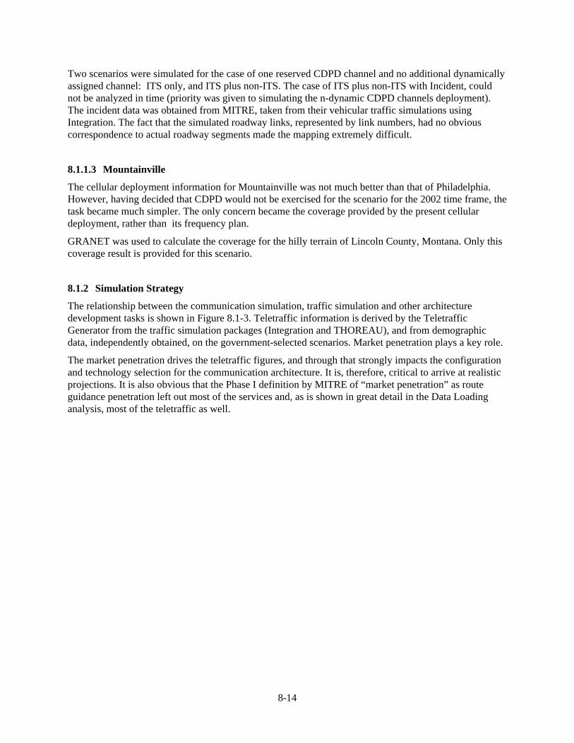
8-14
Two scenarios were simulated for the case of one reserved CDPD channel and no additional dynamicallyassigned channel: ITS only, and ITS plus non-ITS. The case of ITS plus non-ITS with Incident, couldnot be analyzed in time (priority was given to simulating the n-dynamic CDPD channels deployment).The incident data was obtained from MITRE, taken from their vehicular traffic simulations usingIntegration. The fact that the simulated roadway links, represented by link numbers, had no obviouscorrespondence to actual roadway segments made the mapping extremely difficult.
8.1.1.3 Mountainville
The cellular deployment information for Mountainville was not much better than that of Philadelphia.However, having decided that CDPD would not be exercised for the scenario for the 2002 time frame, thetask became much simpler. The only concern became the coverage provided by the present cellulardeployment, rather than its frequency plan.
GRANET was used to calculate the coverage for the hilly terrain of Lincoln County, Montana. Only thiscoverage result is provided for this scenario.
8.1.2 Simulation Strategy
The relationship between the communication simulation, traffic simulation and other architecturedevelopment tasks is shown in Figure 8.1-3. Teletraffic information is derived by the TeletrafficGenerator from the traffic simulation packages (Integration and THOREAU), and from demographicdata, independently obtained, on the government-selected scenarios. Market penetration plays a key role.
The market penetration drives the teletraffic figures, and through that strongly impacts the configurationand technology selection for the communication architecture. It is, therefore, critical to arrive at realisticprojections. It is also obvious that the Phase I definition by MITRE of “market penetration” as routeguidance penetration left out most of the services and, as is shown in great detail in the Data Loadinganalysis, most of the teletraffic as well.

8-15
# Bits/Data FlowData Loading Analysis
Cellular Traffic (non-IVHS)
Government Furnished Information
THOREAU Integration
Route Guidance Penetration
Highway Vehicular Traffic Demographics
Teletraffic Generator
Traffic Simulation
Wireless IVHS Traffic
Communications Architecture
Wireline Alternatives
MOSS * CDPD * CDMA data * GSM data Wireless
Delay/Throuput Statistics
Communication System Simulation
GRANETMap DB
FCC Files
OPNET
Propagation Characteristics
Calibration
WirelessAttributes
Calibration
Overall Delay/Throuput
and other MOE's
Coverage
Map DB
.
Figure 8.1-3 Communication System Simulation/Evaluation Methodology
Preliminary market studies indicate that market penetration will vary significantly by type of service, as itwill vary within a type of service by application or group of applications. The penetration is anticipatedto be high for Commercial Vehicle Operation (CVO), Advanced Public Transit Systems (APTS), andEmergency Vehicle Management (EVM), but significantly smaller for ATIS, even in the 20 year timeframe. This information is covered extensively in the Data Loading section (Section 5), and issummarized for the reader’s convenience in Table 8.1-4 for the 2002 time frame. The ranges showncorrespond to the penetrations for the different applications within a type of service and/or group ofusers.

8-16
Table 8.1-4 Market Penetration Figures Derived from Preliminary Market Studies
2002 PenetrationPersonal Information Access 7 - 10%
Transit Vehicles 10 - 100%Traffic Management 100%
Private Vehicle 7 - 100%Emergency Vehicles 100%
CVO Local 7 - 50%CVO Long Haul 7 - 100%
MOSS was used extensively to simulate CDPD systems using actual cellular deployment informationobtained from FCC filings. At least one CDPD channel per sector was assumed in the urban scenario(i.e., "fully deployed", in a regional, geographic sense). Note that there is no incompatibility between theuse of the term “minimal deployment” (channel-wise) for the case of one reserved CDPD channel persector, and the full geographic deployment nomenclature above.
MOSS uses the ITS teletraffic information from the Teletraffic Generator, as well as cellular non-ITStraffic information (initially voice only, later also non-ITS data), in combination with the wirelessattributes from the Communication Architecture to compute, using the propagation characteristicsobtained from GRANET, delay/throughput statistics for the wireless portion of the communicationsystem.
Besides propagation information, GRANET also provides coverage, C/I, and best server informationbased upon deployment information. This information includes characteristics of the base stations, theirlocations, and the underlying terrain topography, morphology, and land-use/land-cover (partially derivedfrom the latest commercially available GIS data bases).
The reverse link delay characterization obtained from MOSS is then fed into the OPNET protocolsimulation, and also into the wireline simulations. OPNET was already used in Phase I to simulate thewireline network (in fact, the fixed, point-to-point network, since it can also analyze the microwave linksbetween any two nodes), and to perform the comparison of a few technological and topological wirelinealternatives.
To conclude, the outputs of the Communication System Simulation (Figure 8.1-4) are, among others, thequantitative technical MOE’s – Coverage, Delay, Throughput, and information on a link by link levelabout utilization and bandwidth efficiency.

8-17
Traffic &
Communication Simulation
Data Loading
Communications Architecture
Cellular Usage
Gov. Furnished Information
Map DB
FCC Files
# Bits/Data Flow
Attributes
Quantitative Technical MOEs
* Coverage * Delay/Throughput * Utilization * BW Efficiency * ...
Route Guidance Penetration
Figure 8.1-4 Quantitative Technical MOE’s
As in Phase I, system performance is studied during the peak period, and in the case of an incident. Forthe latter, the same approach of analyzing the worst-case incident during the rush hour is followed, nowin with the incident locations chosen by the Government Team. Information on the effect of the incidentswas recently obtained from MITRE (February 1, 1996).
8.1.3 CDPD Protocol Overhead
For convenience, Figure 8.1-5 reproduces the CDPD protocol stack1, since it will enable us to identify allthe steps that introduce overhead. We can begin from the top. Even if outside of the picture, we have thelayers of the protocol above IP, namely TCP (or, better, the transport family of protocols, including inparticular UDP), and the remaining upper layers that we conveniently group as the Application layer.Here we do not account for Application overhead, since it can be included in the message that is passedto the Transport layer (TCP or UDP) which is considered below. In practice, the applications’ developerwill have to address all the details of their overhead to arrive at a successful product.
At the Transport layer, TCP will add 20 bytes of overhead. Note that the TCP payload has to be aninteger number of bytes long – this is the first level that must be quantified, although most applications,especially those generating textual data, already do that. UDP, the other Transport protocol alternativewould only add 8 bytes. Its behavior, however, is quite different from that of TCP. TCP guaranteesdelivery of the messages to the destination, UDP doesn’t.
The reason to maintain TCP here is two-fold: (1) it is our observation that, at the infancy of any service,developers tend to seek the advantage of an application that works as soon as possible – only later, withexperience, will they worry about making it “slick and slim”; (2) by using the larger overhead we are“stretching” as much as possible the communication system under analysis, to obtain conservativeassessments.
1 TCP/IP Illustrated - Vol. I: The Protocols, W. Richard Stevens, Addison-Wesley, 1994.

8-18
N E T W O R K L A Y E R D A T A H E A D E R
H E A D E R CO M P R E S S I O N
D A T A
S E G M E N T 1S E GM E N T 2S E G M E N T 3
E N CR Y P T IO N E N C R Y P T I O N E N C R Y P T I O N
S E G M E N T 1S E G M E N T 2S E G M E N T 3
F R A M I N G
F R A M E 1F R A M E 2F R A M E 3
I N F O R M A T IO N B I T S T R E A M C R E A T I ON
F R A M E 1F R A M E 2F R A M E 3
B L O CK I N G
B L O C K 4 B L O C K 3 B L O C K 2 B L O C K 1F E C 1F E C 2F E C 3F E C 4
N E T W OR K L A Y E R : I P /C L N P
S U B N E T W O R K L A Y E R :S N D C P
L E GE N D
U nmodified Input
M odif ied Input orAdded to Input
CO M P R E S S E DH E A D E R
S E G M E N TH E A D E R
F R A M EH E A D E R
F R A M EF L A G
E N C R Y P T E DD A T A
L I N K L AY E R :M D L P
M A C L A Y E R :D S M A /CD
P H Y S I C A L L A Y E R :G M S K
S E G M E N T A T I O N
P R OCE S S I N G
Figure 8.1-5 CDPD Protocol Stack (Cellular Digital Packet Data System Specification, Release 1.0)
At the Network layer, IP adds another 20 bytes of overhead. Then, at the sub-network layer, SNDCPperforms TCP/IP header compression2. If more than one packet is required in a given transaction,significant header compression gain can be achieved (from 40 to 3 on average). In the case of the widearea ITS applications, almost all the transactions identified thus far require only one packet in eachdirection. No significant gain is thus to be expected from that step.
Next we have the Segmentation and Framing steps. One or two (1-2) additional bytes are added atsegmentation time, and two to six (2-6) additional bytes are added at MDLP framing. Due to systemsettings, 2 bytes are added during segmentation (for non-guaranteed delivery), and we opted to averagethe number of bytes added by MDLP. Hence, we have added a total of 6 bytes during Segmentation andFraming.
2 “Compressing TCP/IP Headers for Low-Speed Serial Links”, V. Jacobson, Network Working Group Request for Comments
1144, Feb. 1990

8-19
Finally, at the MAC layer, during the process of bit stream creation, additional zeros have to beintercalated in the approximately random (due to the previous encryption step) stream of framed data bitsto avoid the accidental occurrence of the Flag or Abort sequence [01111110]. No more than fiveconsecutive 1’s can thus be allowed, which implies that zeros have to be padded as soon as fiveconsecutive 1’s are detected.
The number of zeros thus added to the frame is a random number with a mean that is close to 1.6% of thelength of the message3, although its distribution has a considerable positive tail that can have someimpact, as we will see. It is easy to see that a simple zero added at the wrong time can make it necessaryto use an additional RS-block to carry the message.
When the zero padded bit stream is finally available, different color coding is added for each link (seeFigure 8.1-6), and the bits are prepared to be sent over the mobile link by using a 63/47 Reed-Solomon(RS) error correcting code. The CDPD specification establishes the Reed-Solomon (RS)-block as the“quantum of information” transmitted over the CDPD wireless channel. All messages are carried in aninteger number of RS-blocks, even if they do not fill the “envelope”. This final quantization step has themost significance, since it determines the characteristics of the CDPD traffic (in terms of the proportionof messages being transmitted in a given number of RS-blocks).
3 “The Effects of Zero Padding on the CDPD Wide-Area IVHS Data Load”, Jorge M. Pereira, Personal, Indoors, and Mobile
Communications Conference, PIMRC ‘95, Toronto, Canada, September 26-29, 1995.

8-20
Reed-Solomon (63/47) Block
47 Data Symbols 16 Parity Symbols
Color Code 8-bits
Frame Frame Frame
47 Data Symbols
274 bits 282 bits
Flags Flags Flags FlagsInformation Bistream
Reverse Channel Framing and Block Structure
Forward Channel Framing and Block Structure
Reed-Solomon (63/47) Block
47 Data Symbols 16 Parity Symbols
Color Code 8-bits
Frame Frame Frame
47 Data Symbols
Color Code
274 bits 274 bits
Flags Flags Flags FlagsInformation Bistream
Figure 8.1-6 Framing and Block Structure Showing the Color Code
It is important to point out that from a service and billing perspective, the customer pays per byte and isnot responsible for any network overhead at the IP (network) layer or below. Whatever takes place in theprocess of segmentation, framing, zero padding, or blocking, is completely transparent to the user and hasno impact on the cost of the service. Also, any re-transmissions at any of these lower layers are not theresponsibility of the customer. (These overheads have, nevertheless, an impact on network performance,and that is why they are analyzed here.) The lower layers of the protocol guarantee the error-free deliveryof the message to the MDBS or the M-ES. If that is not possible due to congestion, or repeatedoccurrence of errors during the transmission (39 unsuccessful lower-layer re-transmissions are triedbefore the system quits and warns the upper-layers), then the user does not pay for the undelivered (butlater) delivered bytes.
However, any re-transmissions generated at the higher layers of the protocol, namely by TCP (due totime-outs and lost packets elsewhere in the network), will be of the responsibility of the user, i.e., theuser will have to pay again for the transmitted bytes.

8-21
For the purpose of computing and characterizing the CDPD traffic resulting from the wide area wirelessITS data loading, all the above overhead, and mainly the quantization steps were taken into account. Theresults are presented in the following sections for the two scenarios analyzed for the 2002 time frame.
8.1.4 Non-ITS Applications CDPD Data Loads
In Section 7.3, we concluded that, as a result of the decision to share deployed infrastructure with otherusers, the traffic generated by non-ITS users will have an impact on ITS performance. In that section, weanalyzed in detail the different types of non-ITS traffic to be expected, and came to the conclusion that E-mail and Internet access, the latter dominated by WWW access, would clearly dominate the non-ITStraffic.
The message sizes associated with those two applications were studied in detail, and are reproduced herefor the reader’s convenience. Figure 8.1-7 shows the message distribution for Wireless E-mail Access. E-mail, even if wireless, is a two-way application, so the same distribution applies both in the forward andin the reverse directions. Figure 8.1-8 shows, lacking any more detailed information, the average filetransfer size in bytes, as a function of the time of the day, from a typical WWW server to the user, i.e., inthe forward direction. The reverse direction traffic for Internet access is much smaller, consisting mainlyof transmission of URL’s. Any other traffic is mainly of the E-mail type, especially since e-mailmessages can be sent from the most popular WWW browsers.
0
20
40
60
80
100
120
140
160
0
400
800
1200
1600
2000
2400
2800
3200
3600
4000
4400
4800
Figure 8.1-7 Histogram of Wireless E-mail Message Sizes (up to 5 kbytes)

8-22
MIT WWW Server
7600
7800
8000
8200
8400
8600
8800
9000
0 2 4 6 8 10 12 14 16 18 20 22
Time of Day
Ave
rage
File
Tra
nsfe
r (b
ytes
)
Figure 8.1-8 Average File Transfer Size for the MIT WWW Server (All day Average: 8490 bytes)
In order to approximate the non-ITS traffic, we used the above information to compute the distribution ofthe CDPD packet lengths (in RS-blocks) for the corresponding CDPD traffic. This distribution isirrespective of the total volume, since it relates only to the message sizes involved.
The resulting distribution is shown in Table 8.1-5, independent of the direction.
Table 8.1-5 CDPD Packet Length Distribution for Non-ITS Data
Packet Length (RS-blocks) 1 2 3 4 5Distribution 58.848% 19.616% 13.077% 5.517% 2.942%
We must note here that whereas the distribution may be the same, the actual traffic (volume) in eachdirection will not be. This will be discussed in detail for each scenario under consideration.
8.1.5 CDPD Data Loads
8.1.5.1 Urbansville
8.1.5.1.1 2012 Time Frame, ITS Only, Phase I Data Loads
As discussed in Section 8.1.3, the CDPD specification establishes the Reed-Solomon (RS)-block as thequantum of information transmitted in the radio channel. Thus, for the purposes of network performancesimulation, the transaction lengths determined during the Data Loading analysis in Phase I had to beconverted to the corresponding number of RS-blocks, taking into account the total CDPD protocoloverhead.

8-23
Tables 8.1-6 through 8.1-13 summarize the data load figures for the 2012 time frame, documenting therequired number of RS-blocks per message. The ITS load thus obtained takes into account demographicinformation on Detroit, Michigan DoT information and GTE Mobilnet market analysis. Note that inTable 8.1-9, corresponding to the ITS traffic associated with emergency vehicles, messages with lengthgreater than 6 blocks were split into packets of at most 4 blocks, the industry consensus for optimum (interms of delay/throughput performance) number of blocks per packet.
From Table 8.1-13, it is clear that most of the data load is generated by Local Fleet CommercialVehicles, Private Vehicles, and Probe Vehicles. As expected, the forward link has a somewhat largerdata load than the reverse link. Note that on the forward link, where there is no contention for channelaccess, there is no problem in accommodating the data load – the average channel occupancy is only34.8%, i.e., the forward channel will operate far below capacity. This fact allows for reducing, as a first-cut, the delay in the forward link to queuing delay. As for the reverse channel, due to the inherentcontention mechanism, only simulation can provide the necessary delay/throughput information.
It is noteworthy that the penetration values used in Tables 8.1-6 through 8.1-13 are different (i.e., higher)than those defined in the Market Bundles/Packages Description Blue Book. These “optimistic” valuesresult obviously in upper-bound, worst case data loads relative to what is realistic to expect. However,this margin can compensate both for the anticipated inclusion of additional messages resulting from therefinement of the services definition, and any unanticipated acceptance “take-off” for the 20-year timeframe.
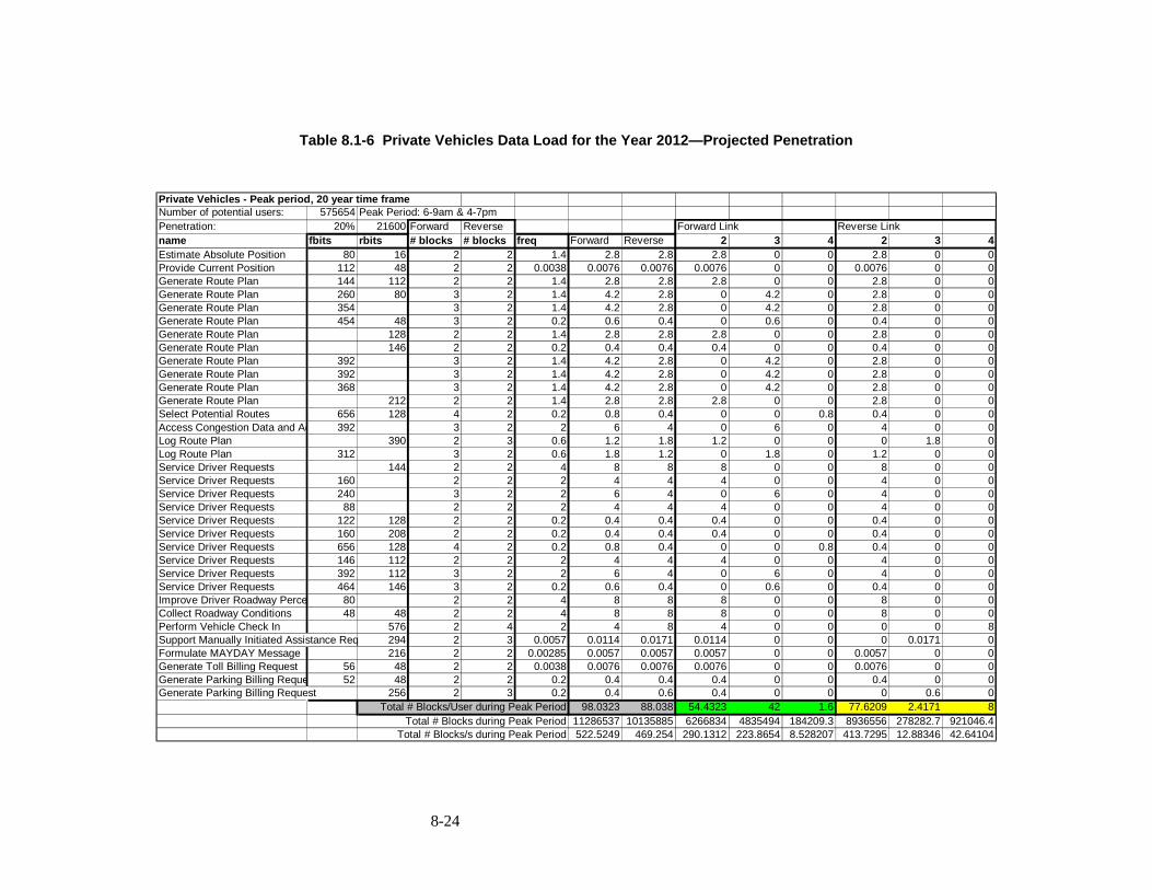
8-24
Table 8.1-6 Private Vehicles Data Load for the Year 2012—Projected Penetration
Private Vehicles - Peak period, 20 year time frameNumber of potential users: 575654 Peak Period: 6-9am & 4-7pmPenetration: 20% 21600 Forward Reverse Forward Link Reverse Linkname fbits rbits # blocks # blocks freq Forward Reverse 2 3 4 2 3 4Estimate Absolute Position 80 16 2 2 1.4 2.8 2.8 2.8 0 0 2.8 0 0Provide Current Position 112 48 2 2 0.0038 0.0076 0.0076 0.0076 0 0 0.0076 0 0Generate Route Plan 144 112 2 2 1.4 2.8 2.8 2.8 0 0 2.8 0 0Generate Route Plan 260 80 3 2 1.4 4.2 2.8 0 4.2 0 2.8 0 0Generate Route Plan 354 3 2 1.4 4.2 2.8 0 4.2 0 2.8 0 0Generate Route Plan 454 48 3 2 0.2 0.6 0.4 0 0.6 0 0.4 0 0Generate Route Plan 128 2 2 1.4 2.8 2.8 2.8 0 0 2.8 0 0Generate Route Plan 146 2 2 0.2 0.4 0.4 0.4 0 0 0.4 0 0Generate Route Plan 392 3 2 1.4 4.2 2.8 0 4.2 0 2.8 0 0Generate Route Plan 392 3 2 1.4 4.2 2.8 0 4.2 0 2.8 0 0Generate Route Plan 368 3 2 1.4 4.2 2.8 0 4.2 0 2.8 0 0Generate Route Plan 212 2 2 1.4 2.8 2.8 2.8 0 0 2.8 0 0Select Potential Routes 656 128 4 2 0.2 0.8 0.4 0 0 0.8 0.4 0 0Access Congestion Data and Ad 392 3 2 2 6 4 0 6 0 4 0 0Log Route Plan 390 2 3 0.6 1.2 1.8 1.2 0 0 0 1.8 0Log Route Plan 312 3 2 0.6 1.8 1.2 0 1.8 0 1.2 0 0Service Driver Requests 144 2 2 4 8 8 8 0 0 8 0 0Service Driver Requests 160 2 2 2 4 4 4 0 0 4 0 0Service Driver Requests 240 3 2 2 6 4 0 6 0 4 0 0Service Driver Requests 88 2 2 2 4 4 4 0 0 4 0 0Service Driver Requests 122 128 2 2 0.2 0.4 0.4 0.4 0 0 0.4 0 0Service Driver Requests 160 208 2 2 0.2 0.4 0.4 0.4 0 0 0.4 0 0Service Driver Requests 656 128 4 2 0.2 0.8 0.4 0 0 0.8 0.4 0 0Service Driver Requests 146 112 2 2 2 4 4 4 0 0 4 0 0Service Driver Requests 392 112 3 2 2 6 4 0 6 0 4 0 0Service Driver Requests 464 146 3 2 0.2 0.6 0.4 0 0.6 0 0.4 0 0Improve Driver Roadway Perce 80 2 2 4 8 8 8 0 0 8 0 0Collect Roadway Conditions 48 48 2 2 4 8 8 8 0 0 8 0 0Perform Vehicle Check In 576 2 4 2 4 8 4 0 0 0 0 8Support Manually Initiated Assistance Req 294 2 3 0.0057 0.0114 0.0171 0.0114 0 0 0 0.0171 0Formulate MAYDAY Message 216 2 2 0.00285 0.0057 0.0057 0.0057 0 0 0.0057 0 0Generate Toll Billing Request 56 48 2 2 0.0038 0.0076 0.0076 0.0076 0 0 0.0076 0 0Generate Parking Billing Reque 52 48 2 2 0.2 0.4 0.4 0.4 0 0 0.4 0 0Generate Parking Billing Request 256 2 3 0.2 0.4 0.6 0.4 0 0 0 0.6 0
Total # Blocks/User during Peak Period 98.0323 88.038 54.4323 42 1.6 77.6209 2.4171 8Total # Blocks during Peak Period 11286537 10135885 6266834 4835494 184209.3 8936556 278282.7 921046.4
Total # Blocks/s during Peak Period 522.5249 469.254 290.1312 223.8654 8.528207 413.7295 12.88346 42.64104

8-25
Table 8.1-7 Long-Haul Freight and Fleet Vehicles Data Load for the Year 2012
Commercial Vehicle - Long Haul, peak period, 20 year time frameNumber of potential users: 7802 Peak Period: 6am-6pmPenetration: 100% 43200 Forward Reverse Forward Link Reverse Linkname fbits rbits # blocks # blocks freq Forward Reverse 2 3 4 2 3 4Disseminate On Board Safety Status 544 2 4 1 2 4 2 0 0 0 0 4Disseminate On Board Safety Status 240 2 3 0.668 1.336 2.004 1.336 0 0 0 2.004 0Disseminate On Board Safety Status 146 2 2 36 72 72 72 0 0 72 0 0Disseminate On Board Safety Status 322 2 3 0.268 0.536 0.804 0.536 0 0 0 0.804 0Disseminate On Board Safety Status 146 2 2 0.167 0.334 0.334 0.334 0 0 0.334 0 0Detect Border Crossing 48 2 2 4 8 8 8 0 0 8 0 0Automatically Log Mileage and Fuel Use 96 2 2 4 8 8 8 0 0 8 0 0Estimate Absolute Position 80 16 2 2 12 24 24 24 0 0 24 0 0Provide Current Position 112 48 2 2 4 8 8 8 0 0 8 0 0Generate Route Plan 144 112 2 2 1.8 3.6 3.6 3.6 0 0 3.6 0 0Generate Route Plan 260 80 3 2 1.8 5.4 3.6 0 5.4 0 3.6 0 0Generate Route Plan 354 3 2 4.2 12.6 8.4 0 12.6 0 8.4 0 0Generate Route Plan 128 2 2 4.2 8.4 8.4 8.4 0 0 8.4 0 0Generate Route Plan 352 3 2 4.2 12.6 8.4 0 12.6 0 8.4 0 0Generate Route Plan 392 3 2 4.2 12.6 8.4 0 12.6 0 8.4 0 0Generate Route Plan 392 3 2 4.2 12.6 8.4 0 12.6 0 8.4 0 0Generate Route Plan 368 3 2 4.2 12.6 8.4 0 12.6 0 8.4 0 0Select Potential Routes 216 2 2 4.2 8.4 8.4 8.4 0 0 8.4 0 0Select Potential Routes 656 128 4 2 0.15 0.6 0.3 0 0 0.6 0.3 0 0Access Congestion Data and Ad 392 3 2 3 9 6 0 9 0 6 0 0Log Route Plan 390 2 3 0.9 1.8 2.7 1.8 0 0 0 2.7 0Log Route Plan 312 3 2 0.9 2.7 1.8 0 2.7 0 1.8 0 0Formulate Route Guidance 392 3 2 3 9 6 0 9 0 6 0 0Service Driver Requests 144 2 2 16 32 32 32 0 0 32 0 0Service Driver Requests 160 2 2 6 12 12 12 0 0 12 0 0Service Driver Requests 392 3 2 2.1 6.3 4.2 0 6.3 0 4.2 0 0Service Driver Requests 88 2 2 12 24 24 24 0 0 24 0 0Service Driver Requests 160 208 2 2 3 6 6 6 0 0 6 0 0Service Driver Requests 146 112 2 2 4 8 8 8 0 0 8 0 0Service Driver Requests 392 112 3 2 6 18 12 0 18 0 12 0 0Service Driver Requests 128 2 2 0.9 1.8 1.8 1.8 0 0 1.8 0 0Disseminate On Board Safety Status 240 2 3 0.668 1.336 2.004 1.336 0 0 0 2.004 0Improve Driver Roadway Perce 80 2 2 6 12 12 12 0 0 12 0 0Collect Roadway Conditions 48 48 2 2 6 12 12 12 0 0 12 0 0Support Manually Initiated Assistance Requ 294 2 3 0.045 0.09 0.135 0.09 0 0 0 0.135 0Formulate MAYDAY Message 216 2 2 0.023 0.046 0.046 0.046 0 0 0.046 0 0Generate Toll Billing Request 56 48 2 2 1 2 2 2 0 0 2 0 0
Total # Blocks/User during Peak Period 369.542 335.946 255.542 113.4 0.6 324.434 7.512 4Total # Blocks during Peak Period 2883167 2621051 1993739 884746.8 4681.2 2531234 58608.62 31208
Total # Blocks/s during Peak Period 66.73997 60.67247 46.15136 20.48025 0.108361 58.59338 1.356681 0.722407

8-26
Table 8.1-8 Local Freight and Fleet Vehicles Data Load for the Year 2012
Commercial Vehicle - Local, peak period, 20 year time frameNumber of potential users: 109182 Peak Period: 6am-6pmPenetration: 60% 43200 Forward Reverse Forward Link Reverse Linkname fbits rbits # blocks # blocks freq Forward Reverse 2 3 4 2 3 4Disseminate On Board Safety Status 544 2 4 1 2 4 2 0 0 0 0 4Disseminate On Board Safety Status 240 2 3 0.668 1.336 2.004 1.336 0 0 0 2.004 0Disseminate On Board Safety Status 146 2 2 36 72 72 72 0 0 72 0 0Disseminate On Board Safety Status 322 2 3 0.268 0.536 0.804 0.536 0 0 0 0.804 0Disseminate On Board Safety Status 146 2 2 0.167 0.334 0.334 0.334 0 0 0.334 0 0Detect Border Crossing 48 2 2 1 2 2 2 0 0 2 0 0Automatically Log Mileage and Fuel Use 96 2 2 1 2 2 2 0 0 2 0 0Estimate Absolute Position 80 16 2 2 12 24 24 24 0 0 24 0 0Provide Current Position 112 48 2 2 0.804 1.608 1.608 1.608 0 0 1.608 0 0Generate Route Plan 144 112 2 2 3.6 7.2 7.2 7.2 0 0 7.2 0 0Generate Route Plan 260 80 3 2 3.6 10.8 7.2 0 10.8 0 7.2 0 0Generate Route Plan 354 3 2 8.4 25.2 16.8 0 25.2 0 16.8 0 0Generate Route Plan 128 2 2 8.4 16.8 16.8 16.8 0 0 16.8 0 0Generate Route Plan 352 3 2 8.4 25.2 16.8 0 25.2 0 16.8 0 0Generate Route Plan 392 3 2 8.4 25.2 16.8 0 25.2 0 16.8 0 0Generate Route Plan 392 3 2 8.4 25.2 16.8 0 25.2 0 16.8 0 0Generate Route Plan 368 3 2 8.4 25.2 16.8 0 25.2 0 16.8 0 0Select Potential Routes 216 2 2 8.4 16.8 16.8 16.8 0 0 16.8 0 0Select Potential Routes 656 128 4 2 0.3 1.2 0.6 0 0 1.2 0.6 0 0Access Congestion Data and Ad 392 3 2 6 18 12 0 18 0 12 0 0Log Route Plan 390 2 3 3.6 7.2 10.8 7.2 0 0 0 10.8 0Log Route Plan 312 3 2 3.6 10.8 7.2 0 10.8 0 7.2 0 0Service Driver Requests 144 2 2 39 78 78 78 0 0 78 0 0Service Driver Requests 160 2 2 12 24 24 24 0 0 24 0 0Service Driver Requests 392 3 2 4.2 12.6 8.4 0 12.6 0 8.4 0 0Service Driver Requests 88 2 2 12 24 24 24 0 0 24 0 0Service Driver Requests 122 128 2 2 1 2 2 2 0 0 2 0 0Service Driver Requests 160 208 2 2 6 12 12 12 0 0 12 0 0Service Driver Requests 656 128 4 2 1 4 2 0 0 4 2 0 0Service Driver Requests 146 112 2 2 2 4 4 4 0 0 4 0 0Service Driver Requests 392 112 3 2 12 36 24 0 36 0 24 0 0Service Driver Requests 128 2 2 6 12 12 12 0 0 12 0 0Disseminate On Board Safety Status 240 2 3 2.4 4.8 7.2 4.8 0 0 0 7.2 0Improve Driver Roadway Perce 80 2 2 4 8 8 8 0 0 8 0 0Collect Roadway Conditions 48 48 2 2 6 12 12 12 0 0 12 0 0Support Manually Initiated Assistance Requ 294 2 3 0.045 0.09 0.135 0.09 0 0 0 0.135 0Formulate MAYDAY Message 216 2 2 0.023 0.046 0.046 0.046 0 0 0.046 0 0Generate Toll Billing Request 56 48 2 2 0.0038 0.0076 0.0076 0.0076 0 0 0.0076 0 0Generate Parking Billing Reque 52 48 2 2 0.1 0.2 0.2 0.2 0 0 0.2 0 0Generate Parking Billing Request 256 2 3 0.2 0.4 0.6 0.4 0 0 0 0.6 0
Total # Blocks/User during Peak Period 542.014 476.95 322.614 214.2 5.2 452.142 20.808 4Total # Blocks during Peak Period 35506904 31244613 21134185 14032071 340647.8 29619461 1363115 262036.8
Total # Blocks/s during Peak Period 821.9191 723.2549 489.2172 324.8165 7.885367 685.6357 31.5536 6.065667

8-27
Table 8.1-9 Emergency Vehicles Data Load for the Year 2012
Emergency Vehicle, p eak period, 20 year time frameNumber of potential users: 3305 Peak Period: 6am-7pmPenetration: 100% 46800 Forward Reverse Forward Link Reverse Linkname fbits rbits # blocks # blocks freq Forward Reverse 2 3 4 2 3 4Present Dispatch Instructions To 2708 12 2 26 52 52 0 0
4 78 312 0 0 312Estimate Absolute Position 80 16 2 2 13 26 26 26 0 0 26 0 0Generate Route Plan 160 112 2 2 2 4 4 4 0 0 4 0 0Generate Route Plan 260 80 3 2 2 6 4 0 6 0 4 0 0Select Potential Routes 656 128 4 2 0.045 0.18 0.09 0 0 0.18 0.09 0 0Access Congestion Data and Ad 392 3 2 2 6 4 0 6 0 4 0 0Log Route Plan 312 3 2 2 6 4 0 6 0 4 0 0Service Driver Requests 144 2 2 6.2 12.4 12.4 12.4 0 0 12.4 0 0Service Driver Requests 160 2 2 2 4 4 4 0 0 4 0 0Service Driver Requests 88 2 2 12 24 24 24 0 0 24 0 0Service Driver Requests 160 208 2 2 0.2 0.4 0.4 0.4 0 0 0.4 0 0Service Driver Requests 146 112 2 2 2 4 4 4 0 0 4 0 0Service Driver Requests 392 112 3 2 2 6 4 0 6 0 4 0 0Disseminate Vehicle and Driver Safety Sta 112 2 2 4 8 8 8 0 0 8 0 0Improve Driver Roadway Perce 80 40 2 2 4 8 8 8 0 0 8 0 0Support Manually Initiated Assistance Requ 294 2 3 0.0019 0.0038 0.0057 0.0038 0 0 0 0.0057 0Formulate MAYDAY Message 216 2 2 0.0019 0.0038 0.0038 0.0038 0 0 0.0038 0 0Communicate Emergency Status 374 2 3 52 104 156 104 0 0 0 156 0Maintain Emergency Vehicle Status 208 2 2 2 4 4 4 0 0 4 0 0Maintain Emergency Vehicle Status 274 2 3 26 52 78 52 0 0 0 78 0Maintain Emergency Vehicle Status 216 2 2 52 104 104 104 0 0 104 0 0Determine Best Vehicle Routes 392 2 3 13 26 39 26 0 0 0 39 0Monitor Emergency Status 1376 2 7 7 14 14 0 0 0 0 0
4 7 28 0 0 283 7 21 0 21 0
Manage Vehicle Dispatch 2708 2 12 6 12 12 0 0 0 0 04 18 72 0 0 0 0 0 72
Total # Blocks/User during Peak Period 742.9876 660.8995 406.8076 24 312.18 266.8938 294.0057 100Total # Blocks during Peak Period 2455574 2184273 1344499 79320 1031755 882084 971688.8 330500
Total # Blocks/s during Peak Period 52.46953 46.6725 28.72861 1.694872 22.04604 18.84795 20.76258 7.061966

8-28
Table 8.1-10 Public Transportation Services Data Load for the Year 2012
Transit Vehicle, peak period, 20 year time frameNumber of potential users: 1789 Peak Period: 6am-7pmPenetration: 100% 46800 Forward Reverse Forward Link Reverse Linkname fbits rbits # blocks # blocks freq Forward Reverse 2 3 4 5 2 3 4Real Time Information Dissemin 656 4 2 26 104 52 0 0 104 0 52 0 0Real Time Information Dissemin 200 2 2 52 104 104 104 0 0 0 104 0 0Real Time Information Dissemin 392 3 2 52 156 104 0 156 0 0 104 0 0Real Time Information Dissemin 656 4 2 52 208 104 0 0 208 0 104 0 0Real Time Information Dissemin 144 2 2 13 26 26 26 0 0 0 26 0 0Report Traffic Information 392 3 2 13 39 26 0 39 0 0 26 0 0Report Traffic Information 272 2 3 13 26 39 26 0 0 0 0 39 0Report Traffic Information 1000 5 2 7 35 14 0 0 0 35 14 0 0Report Vehicle Position Information 48 2 2 78 156 156 156 0 0 0 156 0 0Report Transit Request Information 160 2 2 13 26 26 26 0 0 0 26 0 0Report Transit Request Informa 122 2 2 13 26 26 26 0 0 0 26 0 0Report Transit Request Informa 160 2 2 13 26 26 26 0 0 0 26 0 0Monitor Transit Schedule Adher 24 2 2 13 26 26 26 0 0 0 26 0 0Assess Driver Performance 528 2 4 2 4 8 4 0 0 0 0 0 8Monitor Transit Vehicle Condition 400 2 3 6.24 12.48 18.72 12.48 0 0 0 0 18.72 0Monitor Transit Vehicle Condition 48 2 2 6.24 12.48 12.48 12.48 0 0 0 12.48 0 0Report Passenger Information 160 2 2 26 52 52 52 0 0 0 52 0 0Report Passenger Information 1016 5 2 26 130 52 0 0 0 130 52 0 0Generate Passenger Fare And Loading Sta 160 2 2 78 156 156 156 0 0 0 156 0 0Generate Transit Fare Billing Request 176 2 2 13 26 26 26 0 0 0 26 0 0Generate Transit Fare Billing Request 260 2 3 100 200 300 200 0 0 0 0 300 0Control Passenger Access 88 2 2 100 200 200 200 0 0 0 200 0 0Log Route Plan 312 3 2 26 78 52 0 78 0 0 52 0 0Service Driver Requests 146 2 2 65 130 130 130 0 0 0 130 0 0Service Driver Requests 336 3 2 52 156 104 0 156 0 0 104 0 0Service Driver Requests 88 2 2 13 26 26 26 0 0 0 26 0 0Service Driver Requests 122 128 2 2 13 26 26 26 0 0 0 26 0 0Service Driver Requests 160 208 2 2 13 26 26 26 0 0 0 26 0 0Service Driver Requests 176 2 2 2 4 4 4 0 0 0 4 0 0Improve Driver Roadway Perce 80 2 2 4 8 8 8 0 0 0 8 0 0Determine Longitudinal Collision 48 2 2 2 4 4 4 0 0 0 4 0 0Collect Roadway Conditions 48 48 2 2 4 8 8 8 0 0 0 8 0 0Regulate Lateral Vehicle Contro 18 20 2 2 4 8 8 8 0 0 0 8 0 0Support Manually Initiated Assistance Requ 294 2 3 0.2 0.4 0.6 0.4 0 0 0 0 0.6 0Formulate MAYDAY Message 216 2 2 0.1 0.2 0.2 0.2 0 0 0 0.2 0 0Generate Toll Billing Request 56 48 2 2 0.0038 0.0076 0.0076 0.0076 0 0 0 0.0076 0 0
Total # Blocks/User during Peak Period 2225.568 1951.008 1319.568 429 312 165 1584.688 358.32 8Total # Blocks during Peak Period 3981540 3490353 2360706 767481 558168 295185 2835006 641034.5 14312
Total # Blocks/s during Peak Period 85.07565 74.58018 50.44245 16.39917 11.92667 6.307372 60.57705 13.69732 0.305812

8-29
Table 8.1-11 Traveler Information Services Data Load for the Year 2012
Traveler Information, peak period, 20 year time frameNumber of potential users: 57858 Peak Period: 6-9am &4-7pmPenetration: 20% 21600 Forward Reverse Forward Link Reverse Linkname fbits rbits # blocks # blocks freq Forward Reverse 2 3 4 2 3Reconcile Estimated Position w 24 2 2 0.045 0.09 0.09 0.09 0 0 0.09 0Reconcile Estimated Position w 48 2 2 0.045 0.09 0.09 0.09 0 0 0.09 0Select Potential Routes 216 2 2 2.2 4.4 4.4 4.4 0 0 4.4 0Select Potential Routes 656 4 2 2 8 4 0 0 8 4 0Select Potential Routes 352 3 2 0.2 0.6 0.4 0 0.6 0 0.4 0Access Congestion Data and Ad 392 3 2 1 3 2 0 3 0 2 0Access Congestion Data and Ad 160 2 2 2 4 4 4 0 0 4 0Access Congestion Data and Ad 240 3 2 1 3 2 0 3 0 2 0Access Congestion Data and Ad 392 3 2 0.1 0.3 0.2 0 0.3 0 0.2 0Access Congestion Data and Ad 392 3 2 0.2 0.6 0.4 0 0.6 0 0.4 0Format Traveler Information Request 228 2 2 4.3 8.6 8.6 8.6 0 0 8.6 0Support Manually Initiated Assistance Requ 296 2 3 0.0057 0.0114 0.0171 0.0114 0 0 0 0.0171Transmit MAYDAY Message 216 2 2 0.0057 0.0114 0.0114 0.0114 0 0 0.0114 0
Total # Blocks/User during Peak Period 32.7028 26.2085 17.2028 7.5 8 26.1914 0.0171Total # Blocks during Peak Period 378423.7 303274.3 199063.9 86787 92572.8 303076.4 197.8744
Total # Blocks/s during Peak Period 17.51962 14.04048 9.215922 4.017917 4.285778 14.03132 0.009161

8-30
Table 8.1-12 Probe Vehicles Data Load for the Year 2012
Traffic Management: Probes, peak period, 20 year time frameNumber of potential users: 7704 Peak Period: 6-9am &4-7pmPenetration: 100% 21600 Forward Reverse Forward Reversename fbits rbits # blocks # blocks freq Forward Reverse 2 2 3Probe Trip Notice 464 2 3 2 4 6 4 0 6Probe Trip Accept 64 2 2 2 4 4 4 4 0Probe Report 106 2 2 360 720 720 720 720 0
Total # Blocks/User during Peak Period 728 730 728 724 6Total # Blocks during Peak Period 5608512 5623920 5608512 5577696 46224
Total # Blocks/s during Peak Period 259.6533 260.3667 259.6533 258.2267 2.14

8-31
Table 8.1-13 Overall ITS Data Load Summary for the Year 2012
Peak period, 20 year time frame Forward Link Reverse LinkServices/Users Groupings Forward Reverse 2 3 4 5 2 3 4Transit Vehicles 85.08 74.58 50.44 16.40 11.93 6.31 60.58 13.70 0.31Traveler Information 17.52 14.04 9.22 4.02 4.29 14.03 0.01Traffic Management: P robes 259.65 260.37 259.65 258.23 2.14Private Vehicles 522.52 469.25 290.13 223.87 8.53 413.73 12.88 42.64Emergency Ve hicles 52.47 46.67 28.73 1.69 22.05 18.85 20.76 7.06Commercial V ehicles - Long Haul 66.74 60.67 46.15 20.48 0.11 58.59 1.36 0.72Commercial V ehicles - Local 821.92 723.25 489.22 324.82 7.89 685.64 31.55 6.07
TOTAL # Blocks/s 1825.90 1648.84 1173.54 591.27 54.78 6.31 1509.64 82.40 56.80TOTAL # Blocks/s/sector 16.01668 14.46352
Channel Utilization 34.8% 31.4%Packet Length Distribution 64.3% 32.4% 3.0% 0.3% 91.6% 5.0% 3.4%

8-32
8.1.5.1.2 2002 Time Frame, Phase II Data Loads
8.1.5.1.2.1 ITS OnlyTable 8.1-14 through Table 8.1-21 summarize the data load figures for the 2002 time frame, anddocument the required number of RS-blocks per message.
Two facts should be noted. First, the penetration values used in Table 8.1-14 through Table 8.1-21 arethose defined in the Evaluatory Design document. However, in order to upper-bound, and thus get aworst case CDPD traffic, we assumed that even if there is a competing technology to carry a givenmessage, all the load would be carried over CDPD. As an example, for the traffic between the PIAS andthe ISP, which can either be wireless or wireline, as a worst case assumption, we assumed all of it goingover CDPD. Again, we think this margin is necessary to compensate both for the anticipated inclusion ofadditional messages resulting from the refinement of the services definition, and any unanticipatedacceptance “take-off.”
Second, in spite of the use of worst case traffic, the overall data loads shown in summary Table 8.1-21are still lower than the ones of Phase I, corresponding to Urbansville 2012. This reflects not only a moreconservative approach to ITS service acceptance and adoption rates, but mainly the fact that we are nowlooking at the 2002 time frame instead, where the penetration figures are naturally lower.

8-33
Table 8.1-14 Private Vehicles CDPD Traffic for the Year 2002 Table 8.1-14 Private Vehicles CDPD Traffic f o
Private VehicleNumber of users: 828,947Peak Period: 6-9am &4-7pm 21600 seconds
Forward Reverse Forward Reverse Forward Reverse Frequency* Forward Reverse Forward LinkPA Source PA Sink Penetration Frequency bits bits bytes bytes # blocks # blocks Penetration blocks blocks 1 2 3 4EM VS 10% 0.0001 26 0 6 0 2 0 0.0001 0.0002 0 0 0.0002 0 0EM VS 10% 0.0001 26 0 6 0 2 0 0.0001 0.0002 0 0 0.0002 0 0ISP VS 10% 0.0001 234 0 32 0 3 0 0.0001 0.0003 0 0 0 0.0003 0ISP VS 10% 0.0001 234 0 32 0 3 0 0.0001 0.0003 0 0 0 0.0003 0ISP VS 10% 0.1 6146 0 771 0 24 0 0.1 2.4 0 0 0 0 0ISP VS <34333+22222> 1 1.2 0.4ISP VS 10% 0.01 10802 0 1353 0 41 0 0.01 0.41 0 0 0 0 0ISP VS <2*34333+4332> 0.02 0.3 0.12LocData VS 7% 0.007 146 0 21 0 2 0 0.007 0.014 0 0 0.014 0 0PayInstr VS 10% 0.0001 178 0 25 0 3 0 0.0001 0.0003 0 0 0 0.0003 0PayInstr VS 100% 0.0001 178 0 25 0 3 0 0.0001 0.0003 0 0 0 0.0003 0VS EM 10% 0.0001 0 282 0 38 0 3 0.0001 0 0.0003 0 0 0 0VS EM 10% 0.0001 0 3354 0 422 0 14 0.0001 0 0.0014 0 0 0 0VS EM <333222>VS ISP 10% 0.0001 0 632.4 0 82 0 4 0.0001 0 0.0004 0 0 0 0VS ISP 10% 0.0001 0 642 0 83 0 4 0.0001 0 0.0004 0 0 0 0VS ISP 10% 0.1 0 290 0 39 0 3 0.1 0 0.3 0 0 0 0VS ISP 7% 0.14 0 34 0 7 0 2 0.035 0 0.07 0 0 0 0VS ISP 10% 0.01 0 674 0 87 0 4 0.01 0 0.04 0 0 0 0VS PayInstr 10% 0.0001 0 50 0 9 0 2 0.0001 0 0.0002 0 0 0 0VS PMS 10% 0.00005 0 514 0 67 0 4 0.0001 0 0.0004 0 0 0 0VS PMS 10% 0.00005 0 26 0 6 0 2 0.0001 0 0.0002 0 0 0 0
Total # blocks/User during peak period 0 1.0344 1.5012 0.52*Population 0 857463 1244416 431052.6
/peak period duration 0 39.69736 57.61183 19.95614/per sector 0 0.172597 0.250486 0.086766
packets/s 44.042 5.611 0.00000 19.84868 19.20394 4.989030.0% 45.1% 43.6% 11.3%
Table 8.1-14 Private Vehicles CDPD Traffic for the Year 2002

8-34
Table 8.1-15 Long-Haul Freight and Fleet Vehicles CDPD Traffic for the Year 2002 Table 8.1-15 Long-Haul Freight and Fleet Ve h
CVO Long HaulNumber of users: 6,397Peak Period: 6am-6pm 43200 seconds
Forward Reverse Forward Reverse Forward Reverse Frequency* Forward Reverse Forward LinkPA Source PA Sink Penetration Frequency bits bits bytes bytes # blocks # blocks Penetration blocks blocks 1 2 3 4CVAS CVCS 50% 5E-05 482 0 63 0 4 0 0.0005 0.002 0 0 0 0 0.002CVAS CVCS 50% 0.005 410 0 54 0 3 0 0.05 0.15 0 0 0 0.15 0CVAS CVCS 100% 0.001 410 0 54 0 3 0 0.01 0.03 0 0 0 0.03 0CVAS CVCS 100% 0.001 410 0 54 0 3 0 0.01 0.03 0 0 0 0.03 0CVAS FMS 50% 0.05 26 0 6 0 2 0 0.5 1 0 0 1 0 0CVAS FMS 50% 0.025 3818 0 480 0 16 0 0.25 4 0 0 0 0 0CVAS FMS <34333+2> 0.5 3 1CVAS FMS 50% 0.05 170 0 24 0 3 0 0.5 1.5 0 0 0 1.5 0CVAS FMS 50% 0.025 3818 0 480 0 16 0 0.25 4 0 0 0 0 0CVAS FMS <34333+2> 0.5 3 1CVAS FMS 50% 0.05 346 0 46 0 3 0 0.5 1.5 0 0 0 1.5 0CVCS CVAS 50% 0.005 0 554 0 72 0 4 0.05 0 0.2 0 0 0 0CVCS CVAS 50% 0.0005 0 3362 0 423 0 14 0.005 0 0.07 0 0 0 0CVCS CVAS <333222>CVCS CVAS 100% 0.01 0 554 0 72 0 4 0.1 0 0.4 0 0 0 0CVCS CVAS 100% 0.001 0 538 0 70 0 4 0.01 0 0.04 0 0 0 0CVS FMS 50% 0.5 0 154 0 22 0 2 0.5 0 1 0 0 0 0CVS FMS 50% 0.5 0 330 0 44 0 3 0.5 0 1.5 0 0 0 0CVS FMS 50% 0.5 0 98 0 15 0 2 0.5 0 1 0 0 0 0CVS FMS 50% 1 0 1234 0 157 0 6 1 0 6 0 0 0 0CVS FMS <22111>CVS FMS 50% 0.05 0 26 0 6 0 2 0.05 0 0.1 0 0 0 0CVS FMS 50% 1 0 2066 0 261 0 9 1 0 9 0 0 0 0CVS FMS <22222>EM FMS 10% 1E-05 146 0 21 0 2 0 0.0001 0.0002 0 0 0.0002 0 0EM VS 10% 0.0001 26 0 6 0 2 0 0.0001 0.0002 0 0 0.0002 0 0EM VS 10% 0.0001 26 0 6 0 2 0 0.0001 0.0002 0 0 0.0002 0 0FMS CVAS 50% 0.05 0 402 0 53 0 3 0.5 0 1.5 0 0 0 0FMS CVAS 50% 0.05 0 414 0 54 0 3 0.5 0 1.5 0 0 0 0FMS CVAS 50% 0.05 0 3498 0 440 0 15 0.5 0 7.5 0 0 0 0FMS CVAS <4443>FMS CVAS 50% 0.05 0 414 0 54 0 3 0.5 0 1.5 0 0 0 0FMS CVAS 50% 0.05 0 3498 0 440 0 15 0.5 0 7.5 0 0 0 0FMS CVAS <4443>FMS CVS 50% 0.5 5082 0 638 0 20 0 0.5 10 0 0 0 0 0FMS CVS <34333+2211> 1 2 6 2FMS CVS 50% 0.25 82 0 13 0 2 0 0.25 0.5 0 0 0.5 0 0FMS CVS 50% 0.5 346 0 46 0 3 0 0.5 1.5 0 0 0 1.5 0FMS CVS 50% 1 3042 0 383 0 13 0 1 13 0 0 0 0 0FMS CVS <1/2* 355+1/2*522221> 0.5 4 1.5FMS CVS 50% 1 1226 0 156 0 6 0 1 6 0 0 0 0 0FMS CVS <1/2*33+1/2*22111> 1.5 2 3FMS EM 10% 1E-05 0 3754 0 472 0 16 0.0001 0 0.0016 0 0 0 0FMS EM <34333+2>FMS EM 10% 1E-05 0 242 0 33 0 3 0.0001 0 0.0003 0 0 0 0FMS ImFrghtD 50% 0.005 0 530 0 69 0 4 0.05 0 0.2 0 0 0 0FMS ImFrghtS 50% 0.005 0 530 0 69 0 4 0.05 0 0.2 0 0 0 0FMS ISP 50% 0.05 0 1234 0 157 0 6 0.5 0 3 0 0 0 0FMS ISP <22111>FMS ISP 50% 0.1 0 1354 0 172 0 7 1 0 7 0 0 0 0FMS ISP <421>FMS PayInstr 50% 0.05 0 50 0 9 0 2 0.5 0 1 0 0 0 0ImFrghtD FMS 50% 0.005 530 0 69 0 4 0 0.05 0.2 0 0 0 0 0.2ImFrghtS FMS 50% 0.005 530 0 69 0 4 0 0.05 0.2 0 0 0 0 0.2ISP FMS 50% 0.05 3034 0 382 0 13 0 0.5 6.5 0 0 0 0 0ISP FMS <522221> 0.5 4ISP FMS 50% 0.1 3154 0 397 0 13 0 1 13 0 0 0 0 0ISP FMS <43322> 4 6 4ISP VS 10% 0.0001 234 0 32 0 3 0 0.0001 0.0003 0 0 0 0.0003 0ISP VS 10% 0.0001 234 0 32 0 3 0 0.0001 0.0003 0 0 0 0.0003 0ISP VS 10% 0.1 6146 0 771 0 24 0 0.1 2.4 0 0 0 0 0ISP VS <34333+22222> 1 1.2 0.4ISP VS 10% 0.01 10802 0 1353 0 41 0 0.01 0.41 0 0 0 0 0ISP VS <2*34333+1/2*5322+1/2*4332> 0.03 0.285 0.1LocData VS 7% 0.007 146 0 21 0 2 0 0.007 0.014 0 0 0.014 0 0PayInstr FMS 50% 0.05 114 0 17 0 2 0 0.5 1 0 0 1 0 0PayInstr VS 10% 0.0001 178 0 25 0 3 0 0.0001 0.0003 0 0 0 0.0003 0
Table 8.1-15 Long-Haul Freight and Fleet Vehicles CDPD Traffic for the Year 2002

8-35
Table 8.1-16 Local Freight and Fleet Vehicles CDPD Traffic for the Year 2002 Table 8.1-16 Local Freight and Fleet Vehicle s
CVO LocalNumber of users: 89,565Peak Period: 6am-6pm 43200 seconds
Forward Reverse Forward Reverse Forward Reverse Frequency* Forward Reverse Forward LinkPA Source PA Sink Penetration Frequency bits bits bytes bytes # blocks # blocks Penetration blocks blocks 1 2 3 4CVS FMS 50% 1 0 154 0 22 0 2 1 0 2 0 0 0 0CVS FMS 50% 2 0 1234 0 157 0 6 1.5 0 9 0 0 0 0CVS FMS <22111>CVS FMS 50% 0.05 0 26 0 6 0 2 0.05 0 0.1 0 0 0 0CVS FMS 50% 2 0 2066 0 261 0 9 2 0 18 0 0 0 0CVS FMS <22222>EM FMS 10% 1E-05 146 0 21 0 2 0 0.0001 0.0002 0 0 0.0002 0 0EM VS 10% 0.0001 26 0 6 0 2 0 0.0001 0.0002 0 0 0.0002 0 0EM VS 10% 0.0001 26 0 6 0 2 0 0.0001 0.0002 0 0 0.0002 0 0FMS CVS 50% 1 5082 0 638 0 20 0 1 20 0 0 0 0 0FMS CVS <34333+2211> 2 4 12 4FMS CVS 50% 2 3042 0 383 0 13 0 2 26 0 0 0 0 0FMS CVS <355> 6FMS CVS 50% 2 1226 0 156 0 6 0 2 12 0 0 0 0 0FMS CVS <22111> 6 8FMS EM 10% 1E-05 0 3754 0 472 0 16 0.0001 0 0.0016 0 0 0 0FMS EM <34333+2>FMS EM 10% 1E-05 0 242 0 33 0 3 0.0001 0 0.0003 0 0 0 0FMS ImFrghtD 50% 0.005 0 530 0 69 0 4 0.05 0 0.2 0 0 0 0FMS ImFrghtS 50% 0.005 0 530 0 69 0 4 0.05 0 0.2 0 0 0 0FMS ISP 50% 0.1 0 1234 0 157 0 6 1 0 6 0 0 0 0FMS ISP <22111>FMS ISP 50% 0.2 0 1354 0 172 0 7 2 0 14 0 0 0 0FMS ISP <421>ImFrghtD FMS 50% 0.005 530 0 69 0 4 0 0.05 0.2 0 0 0 0 0.2ImFrghtS FMS 50% 0.005 530 0 69 0 4 0 0.05 0.2 0 0 0 0 0.2ISP FMS 50% 0.1 3034 0 382 0 13 0 1 13 0 0 0 0 0ISP FMS <522221> 1 8ISP FMS 50% 0.2 3154 0 397 0 13 0 2 26 0 0 0 0 0ISP FMS <1/2*43322+1/2*24422> 10 6 12ISP VS 10% 0.0001 234 0 32 0 3 0 0.0001 0.0003 0 0 0 0.0003 0ISP VS 10% 0.0001 234 0 32 0 3 0 0.0001 0.0003 0 0 0 0.0003 0ISP VS 10% 0.2 6146 0 771 0 24 0 0.2 4.8 0 0 0 0 0ISP VS <34333+22222> 2 2.4 0.8ISP VS 10% 0.01 10802 0 1353 0 41 0 0.01 0.41 0 0 0 0 0ISP VS <2*34333+5322> 0.04 0.27 0.08LocData VS 7% 0.007 146 0 21 0 2 0 0.007 0.014 0 0 0.014 0 0PayInstr VS 10% 0.0001 178 0 25 0 3 0 0.0001 0.0003 0 0 0 0.0003 0VS EM 10% 0.0001 0 282 0 38 0 3 0.0001 0 0.0003 0 0 0 0VS EM 10% 0.0001 0 3354 0 422 0 14 0.0001 0 0.0014 0 0 0 0VS EM <333222>VS ISP 10% 0.0001 0 632.4 0 82 0 4 0.0001 0 0.0004 0 0 0 0VS ISP 10% 0.0001 0 642 0 83 0 4 0.0001 0 0.0004 0 0 0 0VS ISP 10% 0.2 0 290 0 39 0 3 0.2 0 0.6 0 0 0 0VS ISP 10% 0.01 0 674 0 87 0 4 0.01 0 0.04 0 0 0 0VS PayInstr 10% 0.0001 0 50 0 9 0 2 0.0001 0 0.0002 0 0 0 0VS PMS 10% 0.00005 0 514 0 67 0 4 0.0001 0 0.0004 0 0 0 0VS PMS 10% 0.00005 0 26 0 6 0 2 0.0001 0 0.0002 0 0 0 0
Total # blocks/User during peak period 9 32.0546 26.6709 17.28*Population 806084.1749 2870967 2388777 1547682
/peak period duration 18.6593559 66.45758 55.29576 35.82596/per sector 0.081127634 0.288946 0.240416 0.155765
packets/s 89.664 61.912 18.65936 33.22879 18.43192 8.9564920.8% 37.1% 20.6% 10.0%
Table 8.1-16 Local Freight and Fleet Vehicles CDPD Traffic for the Year 2002

8-36
Table 8.1-17 Emergency Vehicles CDPD Traffic for the Year 2002 Table 8.1-17 Emergency Vehicles CDPD Traf f
Emergency VehicleNumber of users: 4,850Peak Period: 6am-7pm 46800 seconds
Forward Reverse Forward Reverse Forward Reverse Frequency* Forward Reverse Forward LinkPA Source PA Sink Penetration Frequency bits bits bytes bytes # blocks # blocks Penetration blocks blocks 1 2 3 4EM EVS 100% 13 1042 0 133 0 6 0 13 78 0 0 0 0 0EM EVS <411> 26 52EVS EM 100% 26 0 26 0 6 0 2 26 0 52 0 0 0 0EVS EM 100% 26 0 146 0 21 0 2 26 0 52 0 0 0 0EVS EM 100% 13 0 530 0 69 0 4 13 0 52 0 0 0 0
Total # blocks/User during peak period 26 0 0 52*Population 126093.5221 0 0 252187
/peak period duration 2.694306027 0 0 5.388612/per sector 0.011714374 0 0 0.023429
packets/s 4.041 6.736 2.69431 0.00000 0.00000 1.3471566.7% 0.0% 0.0% 33.3%
Table 8.1-17 Emergency Vehicles CDPD Traffic for the Year 2002

8-37
Table 8.1-18 Transit Vehicles CDPD Traffic for the Year 2002 Table 8.1-18 Transit Vehicles CDPD Traffic f o
Transit VehiclesPublic_Transit_Vehicles1466 Peak Period: 6am-7pm 46800 seconds
ParaTransit_Vehicles367Transit Customers47,440 Forward Reverse Forward Reverse Forward Reverse Frequency* Forward Reverse Forward Link
PA Source PA Sink Penetration Frequency bits bits bytes bytes # blocks # blocks Penetration blocks blocks 1 2 3 4ISP RTS 10% 0.00032 426 0 56 0 3 0 0.003236016 0.00971 0 0 0 0.009708 0ISP RTS 10% 0.00032 666 0 86 0 4 0 0.003236016 0.01294 0 0 0 0 0.012944ISP RTS 10% 0.00032 498 0 65 0 4 0 0.003236016 0.01294 0 0 0 0 0.012944ISP RTS 10% 0.00032 987.68 0 126 0 5 0 0.003236016 0.01618 0 0 0 0 0PayInstr RTS 10% 0.064 26 0 6 0 2 0 0.647203274 1.29441 0 0 1.294407 0 0PayInstr RTS 10% 0.00032 178 0 25 0 3 0 0.003236016 0.00971 0 0 0 0.009708 0PayInstr RTS 10% 0.00032 178 0 25 0 3 0 0.003236016 0.00971 0 0 0 0.009708 0PayInstr RTS 10% 0.00032 178 0 25 0 3 0 0.003236016 0.00971 0 0 0 0.009708 0PayInstr TRVS 100% 32 26 0 6 0 2 0 32.36016371 64.7203 0 0 64.72033 0 0PayInstr TRVS 100% 0.032 178 0 25 0 3 0 0.032360164 0.09708 0 0 0 0.09708 0RTS EM 100% 0.0032 0 370 0 49 0 3 0.032360164 0 0.09708 0 0 0 0RTS ISP 10% 0.00032 0 738 0 95 0 5 0.003236016 0 0.01618 0 0 0 0RTS ISP 10% 0.320000005 0 98 0 15 0 2 3.236016371 0 6.47203 0 0 0 0RTS ISP 10% 0.064000001 0 66 0 11 0 2 0.647203274 0 1.29441 0 0 0 0RTS ISP 10% 0.320000005 0 58 0 10 0 2 3.236016371 0 6.47203 0 0 0 0RTS ISP 10% 0.00032 0 978 0 125 0 5 0.003236016 0 0.01618 0 0 0 0RTS ISP 10% 0.00032 0 402 0 53 0 3 0.003236016 0 0.00971 0 0 0 0RTS ISP 10% 0.00032 0 858 0 110 0 5 0.003236016 0 0.01618 0 0 0 0RTS ISP 10% 0.00032 0 1434 0 182 0 7 0.003236016 0 0.02265 0 0 0 0RTS ISP <34>RTS ISP 10% 0.00032 0 26 0 6 0 2 0.003236016 0 0.00647 0 0 0 0RTS PayInstr 10% 0.064000001 0 50 0 9 0 2 0.647203274 0 1.29441 0 0 0 0RTS PayInstr 10% 0.032 0 50 0 9 0 2 0.323601637 0 0.6472 0 0 0 0RTS PayInstr 10% 0.00032 0 50 0 9 0 2 0.003236016 0 0.00647 0 0 0 0RTS PayInstr 10% 0.00032 0 34 0 7 0 2 0.003236016 0 0.00647 0 0 0 0TRMS TRVS 100% 0.1 8210 0 1029 0 32 0 0.1 3.2 0 0 0 0 0TRMS TRVS <2*34333+2> 0.2 2.4 0.8TRMS TRVS 100% 32 26 0 6 0 2 0 32.36016371 64.7203 0 0 64.72033 0 0TRMS TRVS 10% 0.0032 2418 0 305 0 11 0 0.003236016 0.0356 0 0 0 0 0TRMS TRVS <3332> 0.006472 0.029124TRMS TRVS 100% 13 1042 0 133 0 6 0 13.01773533 78.1064 0 0 0 0 0TRMS TRVS <411> 26.03547067 52.07094TRMS TRVS 100% 0.032 82 0 13 0 2 0 0.032360164 0.06472 0 0 0.06472 0 0TRMS TRVS 100% 0.032 34 0 7 0 2 0 0.032360164 0.06472 0 0 0.06472 0 0TRMS TRVS 100% 13 17260 0 2160 0 65 0 13 845 0 0 0 0 0TRMS TRVS <4*34333+5> 624.00 208.00TRMS TRVS 100% 52 7786 0 976 0 30 0 52 1560 0 0 0 0 0TRMS TRVS <34333+43333> 1248 416TRMS TRVS 100% 1 16826 0 2106 0 63 0 0.541666667 34.125 0 0 0 0 0TRMS TRVS <4*34333+5> 26.00 8.67TRMS TRVS 100% 0.032 554 0 72 0 4 0 0.032360164 0.12944 0 0 0 0 0.129441TRMS TRVS 100% 1 922 0 118 0 5 0 1 5 0 0 0 0 0TRMS TRVS 100% 32 26 0 6 0 2 0 32.36016371 64.7203 0 0 64.72033 0 0TRMS TRVS 100% 32 34 0 7 0 2 0 32.36016371 64.7203 0 0 64.72033 0 0TRVS PayInstr 100% 32 0 50 0 9 0 2 32.36016371 0 64.7203 0 0 0 0TRVS PayInstr 100% 32 0 34 0 7 0 2 32.36016371 0 64.7203 0 0 0 0TRVS TRMS 10% 0.0032 0 2418 0 305 0 11 0.003236016 0 0.0356 0 0 0 0TRVS TRMS <3332>TRVS TRMS 100% 13 0 26 0 6 0 2 52 0 104 0 0 0 0TRVS TRMS 100% 32 0 466 0 61 0 4 32.36016371 0 129.441 0 0 0 0TRVS TRMS 100% 0.1 0 34 0 7 0 2 0.1 0 0.2 0 0 0 0TRVS TRMS 100% 0.0032 0 282 0 38 0 3 0.003236016 0 0.00971 0 0 0 0TRVS TRMS 100% 0.0032 0 282 0 38 0 3 0.003236016 0 0.00971 0 0 0 0TRVS TRMS 100% 0.0032 0 1042 0 133 0 6 0.003236016 0 0.01942 0 0 0 0TRVS TRMS <411>TRVS TRMS 100% 3.2 0 186 0 26 0 3 3.236016371 0 9.70805 0 0 0 0TRVS TRMS 100% 0.011 0 73746 0 9221 0 271 0.013642565 0 3.69714 0 0 0 0TRVS TRMS <18*34333+3>TRVS TRMS 10% 0.0032 0 1450 0 184 0 7 0.003236016 0 0.02265 0 0 0 0TRVS TRMS <34>TRVS TRMS 100% 13 0 1042 0 133 0 6 13 0 78 0 0 0 0TRVS TRMS <411>TRVS TRMS 100% 13 0 1826 0 231 0 9 13 0 117 0 0 0 0TRVS TRMS <4221>TRVS TRMS 100% 52 0 274 0 37 0 3 52 0 156 0 0 0 0TRVS TRMS 100% 156 0 234 0 32 0 3 156 0 468 0 0 0 0TRVS TRMS 100% 32 0 26 0 6 0 2 32.36016371 0 64.7203 0 0 0 0
Table 8.1-18 Transit Vehicles CDPD Traffic for the Year 2002

8-38
Table 8.1-19 Personal Information Access CDPD Traffic for the Year 2002 Table 8.1-19 Personal Information Access C D
Personal Information Access Peak Period: 6-9am & 4-7pm 21600 secondsUniverse 876,390 Remote Access Users87,639
Mobile (Profissional) Penetration10% Forward Reverse Forward Reverse Forward Reverse Frequency* Forward Reverse Forward LinkPA Source PA Sink Penetration Frequency bits bits bytes bytes # blocks # blocks Penetration blocks blocks 1 2 3 4EM PIAS 10% 0.000025 26 0 6 0 2 0 0.00005 0.0001 0 0 0.0001 0 0ISP PIAS 10% 0.00025 3578 0 450 0 15 0 0.005 0.075 0 0 0 0 0ISP PIAS <532222> 0.04 0.015ISP PIAS 7% 0.0035 18306 0 2291 0 69 0 0.07 4.83 0 0 0 0 0ISP PIAS <4x43333 + 45> 3.36 1.4ISP PIAS 10% 0.005 818 0 105 0 5 0 0.01 0.05 0 0 0 0 0ISP PIAS 10% 0.005 650 0 84 0 4 0 0.01 0.04 0 0 0 0 0.04ISP PIAS 10% 0.05 1139.7 0 145 0 6 0 0.1 0.6 0 0 0 0 0ISP PIAS <51> 0.1LocData PIAS 7% 0.007 146 0 21 0 2 0 0.007 0.014 0 0 0.014 0 0PayInstr PIAS 10% 0.005 178 0 25 0 3 0 0.01 0.03 0 0 0 0.03 0PIAS EM 10% 0.000025 0 370 0 49 0 3 0.00005 0 0.00015 0 0 0 0PIAS ISP 10% 0.05 0 250 0 34 0 3 0.1 0 0.3 0 0 0 0PIAS ISP 10% 0.0025 0 250 0 34 0 3 0.005 0 0.015 0 0 0 0PIAS ISP 10% 0.05 0 210 0 29 0 3 0.1 0 0.3 0 0 0 0PIAS ISP 10% 0.005 0 1130 0 144 0 6 0.01 0 0.06 0 0 0 0PIAS ISP <51>PIAS ISP 10% 0.005 0 402 0 53 0 3 0.01 0 0.03 0 0 0 0PIAS ISP 10% 0.05 0 26 0 6 0 2 0.1 0 0.2 0 0 0 0PIAS PayInstr 10% 0.005 0 50 0 9 0 2 0.01 0 0.02 0 0 0 0PIAS TRMS 10% 0.005 0 466 0 61 0 4 0.01 0 0.04 0 0 0 0TRMS PIAS 10% 0.00165 2530 0 319 0 11 0 0.005 0.055 0 0 0 0 0TRMS PIAS <222222> 0.06
Total # blocks/User during peak period 0.1 0.1141 3.405 1.44*Population 8763.9 9999.61 298410.8 126200.2
/peak period duration 0.405736111 0.462945 13.81531 5.8426/per sector 0.00176407 0.002013 0.060067 0.025403
packets/s 7.454 1.441 0.40574 0.23147 4.60510 1.460655.4% 3.1% 61.8% 19.6%
Table 8.1-19 Personal Information Access CDPD Traffic for the Year 2002

8-39
Table 8.1-20 Probe Vehicles CDPD Traffic for the Year 2002 Table 8.1-20 Probe Vehicles CDPD Traffic fo r
Trafic Management = ProbesNumber of users: 7,704Peak Period: 6-9am & 4-7pm 21600 seconds
Forward Reverse Forward Reverse Forward Reverse Frequency* Forward Reverse Forward LinkPA Source PA Sink Penetration Frequency bits bits bytes bytes # blocks # blocks Penetration blocks blocks 1 2 3 4VS ISP 100% 12 0 314 0 42 0 3 12 0 36 0 0 0
Total # blocks/User during peak period 0 0 0*Population 0 0 0
/peak period duration 0 0 0/per sector 0 0 0
packets/s 0.000 4.280 0.00000 0.00000 0.00000 0.00000
Table 8.1-20 Probe Vehicles CDPD Traffic for the Year 2002 , Urbansville
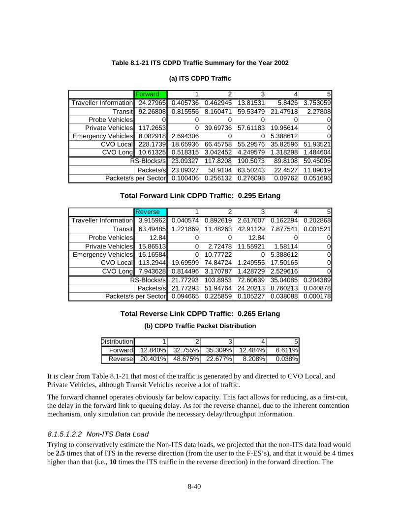
8-40
Table 8.1-21 ITS CDPD Traffic Summary for the Year 2002
(a) ITS CDPD Traffic
Forward 1 2 3 4 5Traveller Information 24.27965 0.405736 0.462945 13.81531 5.8426 3.753059
Transit 92.26808 0.815556 8.160471 59.53479 21.47918 2.27808Probe Vehicles 0 0 0 0 0 0
Private Vehicles 117.2653 0 39.69736 57.61183 19.95614 0Emergency Vehicles 8.082918 2.694306 0 0 5.388612 0
CVO Local 228.1739 18.65936 66.45758 55.29576 35.82596 51.93521CVO Long 10.61325 0.518315 3.042452 4.249579 1.318298 1.484604
RS-Blocks/s 23.09327 117.8208 190.5073 89.8108 59.45095Packets/s 23.09327 58.9104 63.50243 22.4527 11.89019
Packets/s per Sector 0.100406 0.256132 0.276098 0.09762 0.051696
Total Forward Link CDPD Traffic: 0.295 Erlang
Reverse 1 2 3 4 5Traveller Information 3.915962 0.040574 0.892619 2.617607 0.162294 0.202868
Transit 63.49485 1.221869 11.48263 42.91129 7.877541 0.001521Probe Vehicles 12.84 0 0 12.84 0 0
Private Vehicles 15.86513 0 2.72478 11.55921 1.58114 0Emergency Vehicles 16.16584 0 10.77722 0 5.388612 0
CVO Local 113.2944 19.69599 74.84724 1.249555 17.50165 0CVO Long 7.943628 0.814496 3.170787 1.428729 2.529616 0
RS-Blocks/s 21.77293 103.8953 72.60639 35.04085 0.204389Packets/s 21.77293 51.94764 24.20213 8.760213 0.040878
Packets/s per Sector 0.094665 0.225859 0.105227 0.038088 0.000178
Total Reverse Link CDPD Traffic: 0.265 Erlang
(b) CDPD Traffic Packet Distribution
Distribution 1 2 3 4 5Forward 12.840% 32.755% 35.309% 12.484% 6.611%Reverse 20.401% 48.675% 22.677% 8.208% 0.038%
It is clear from Table 8.1-21 that most of the traffic is generated by and directed to CVO Local, andPrivate Vehicles, although Transit Vehicles receive a lot of traffic.
The forward channel operates obviously far below capacity. This fact allows for reducing, as a first-cut,the delay in the forward link to queuing delay. As for the reverse channel, due to the inherent contentionmechanism, only simulation can provide the necessary delay/throughput information.
8.1.5.1.2.2 Non-ITS Data LoadTrying to conservatively estimate the Non-ITS data loads, we projected that the non-ITS data load wouldbe 2.5 times that of ITS in the reverse direction (from the user to the F-ES’s), and that it would be 4 timeshigher than that (i.e., 10 times the ITS traffic in the reverse direction) in the forward direction. The

8-41
reason for this different treatment is that, as we have already discussed, the reverse direction traffic ismostly due to E-mail, while the forward traffic consists mainly of E-mail and WWW Access, with itsassociated downloads, and is therefore expected to be much larger.
The resulting traffic for Urbansville 2002 is, therefore, as shown in Table 8.1-22.
Table 8.1-22 Non-ITS CDPD Traffic
Non-ITS Traffic Forward 1 2 3 4 5 RS-Blocks/s per Sector 3.3724 2.248267 2.248267 1.26465 0.8431
Packets/s per Sector 3.3724 1.124133 0.749422 0.316163 0.16862Reverse 1 2 3 4 5
RS-Blocks/s per Sector 0.8431 0.562067 0.562067 0.316163 0.210775Packets/s per Sector 0.8431 0.281033 0.187356 0.079041 0.042155
The distribution, as was discussed before, is taken to be the same in both directions. The resulting overalltraffic follows in Table 8.1-23.
Table 8.1-23 Overall ITS plus Non-ITS CDPD Traffic
Total Traffic Forward 1 2 3 4 5 RS-Blocks/s per Sector 3.472806 2.760531 3.076559 1.655132 1.101582
Packets/s per Sector 3.472806 1.380266 1.02552 0.413783 0.220316Distribution 53.324% 21.193% 15.746% 6.353% 3.383%Reverse 1 2 3 4 5
RS-Blocks/s per Sector 0.937765 1.013785 0.877747 0.468514 0.211664Packets/s per Sector 0.937765 0.506893 0.292582 0.117129 0.042333
Distribution 49.442% 26.725% 15.426% 6.175% 2.232%
8.1.5.1.2.3 Incident CaseThe incident case for Urbansville was defined by MITRE. Unfortunately, at the time when theinformation was requested, all the simulation files obtained from Integration had already been erased.Given time constraints, it was not possible to re-run Integration for the Urbansville scenario, and theinformation provided to the Joint Team (February 1, 1996) was the following:
1. Incident occurring at the intersection of Ford and Lodge freeways in downtown Detroit, in thedirection E-W, affecting approximately 2.5 miles of freeway. This information was used to concludethat two sectors would be affected by the incident, namely Tiger Stadium #1, and Baltimore #3.Furthermore, most of the congestion occurs within the Tiger Stadium #1 sector.
a) Number of vehicles in the most affected sector under normal peak period traffic conditions: 4905.
b) Number of vehicles in the most affected sector immediately before the incident began to clear:7256.

8-42
In order to analyze a worst case scenario, we assumed that all the vehicles identified as being in the mostaffected sector were in the affected link of freeway. Furthermore, we assumed that all those vehicles,independent of their direction, would be affected. (In reality, assuming equilibrium during the peakperiod, only approximately 4800 [~ 7256-(4905/2)] vehicles are affected by the incident). As such, wehave maximized the CDPD traffic increase due to the incident, i.e., its impact on CDPD performance (seeFigure 8.1-9).

8-43
*
Figure 8.1-9 Location of the Incident showing the Sectors Involved, as well as the Sectors andRoadway Segments Affected by the Incident

8-44
8.1.5.2 Thruville 2002
It should be noted that the Data Loading analysis in this document, as well as the Evaluatory Designdocument, looked at only the New Jersey side of Thruville. Given that our cellular deployment extendedinto the Pennsylvania side, where Philadelphia is located, we had to extend the population figuresconsidered therein to account for the whole scenario.
In any case, as it is very easy to observe, the ITS traffic considered for Thruville is quite different fromthat analyzed for Urbansville. This stems, as explained in the Evaluatory Design document, from thedifferent set of ITS services scheduled for deployment in this inter-urban scenario.
8.1.5.2.1 ITS only
Table 8.1-24 through Table 8.1-31 summarize the data load for the 2002 time frame for Thruville(Philadelphia-Trenton corridor). As shown In Table 8.1-31, the data loads are now significantly smallerthen those in Detroit, given that a smaller set of ITS services will be deployed at that time.

Table 8.1-24 Private Vehicles CDPD Traffic for the Year 2002
Private Vehicle 1.086276259 Factor due to through trafficNumber of users: 3,202,686 Penetration
Peak Period: 6-9am/4-7pm 7%21600 s 100% (DL Freq) *
PA Source PA Sink Physical Data Flow Penetration Penetration 1/(DL Freq) Explanation NumberEM VS emergency_request_driver_acknowledge 10% 0.0001 1000 one emergency per 1000 vehicles 1000EM VS emergency_request_vehicle_acknowledge 10% 0.0001 1000 one emergency per 1000 vehicles 1000LocData VS From_Location_Data_Source 7% 0.007 10 one in 10 vs 10PayInstr VS fpi_transit_user_vehicle_input_credit_identity 100% 0.0001 10000 one in 10000 vehicles this flow 10000VS EM emergency_request_driver_details 10% 0.0001 1000 one emergency per 1000 vehicles 1000VS EM emergency_request_vehicle_details 10% 0.0001 1000 one emergency per 1000 vehicles 1000
VS ISP advisory_data_request 10% 0.1 1 one request per vehicle 1VS ISP vehicle_guidance_route_accepted 7% 0.14 1/2 two acceptances 1/2
W.C. Forward Reverse Forward Reverse Forward Reverse Frequency* Forward Reverse Forward Link Reverse LinkFactor bits bits bytes bytes # blocks # blocks Penetration blocks blocks 1 2 3 4 5 1 2 3
1 26 0 6 0 2 0 0.0001 0.0002 0 0.0002 0 0 0 0 01 26 0 6 0 2 0 0.0001 0.0002 0 0.0002 0 0 0 0 01 146 0 21 0 2 0 0.007 0.014 0 0.014 0 0 0 0 01 178 0 25 0 3 0 0.0001 0.0003 0 0 0.0003 0 0 0 01 0 282 0 38 0 3 0.0001 0 0.0003 0 0 0 0 0 0.00031 0 3354 0 422 0 14 0.0001 0 0.0014 0 0 0 0 0 0
<53322> 0.0004 0.00061 0 290 0 39 0 3 0.1 0 0.3 0 0 0 0 0 0.31 0 34 0 7 0 2 0.14 0 0.28 0 0 0 0 0.28 0
Total # blocks/User 0 0.0144 0.0003 0 0 0 0.2804 0.3009*Population 0 50097.63 1043.701 0 0 0 975512.1 1046832
/peak period duration 0 2.319335 0.048319 0 0 0 45.1626 48.46443/per sector 0 0.010084 0.00021 0 0 0 0.196359 0.210715
8-45

Table 8.1-25 Long-Haul Freight and Fleet Vehicles CDPD Traffic for the Year 2002 Table 8.1-25 Long-Haul Freight and Fleet Vehicles CDPD Traffic for the Year 2002
CVO Long Haul 1.0862763 Factor due to through trafficNumber of users: 24,717 Penetration 50% of LH Trucks operating in a Metro Area
Peak Period: 43200 7% 6am-6pm (12 hours) 100% (DL Freq) * W.C. Forward Reverse Forward Reverse Forward Reverse Frequency* Forward Reverse Forward Link Reverse Link
PA Source PA Sink Physical Data Flow Penetration Penetration 1/(DL Freq) Explanation Number Factor bits bits bytes bytes # blocks # blocks Penetration blocks blocks 1 2 3 4 5 1 2 3 4 5CVAS CVCS cv_credentials_database_update 50% 0.00005 10000 1 out of 1000 vehicles 1000 10 482 0 63 0 4 0 0.0005 0.002 0 0 0 0.002 0 0 0 0 0CVAS CVCS cv_credentials_information_response 50% 0.005 100 1 out of 10 vehicles 10 10 410 0 54 0 3 0 0.05 0.15 0 0 0.15 0 0 0 0 0 0CVAS CVCS cv_safety_database_update 100% 0.001 1000 1 out of 100 vehicles 100 10 410 0 54 0 3 0 0.01 0.03 0 0 0.03 0 0 0 0 0 0CVAS CVCS cv_safety_information_response 100% 0.001 1000 1 out of 100 vehicles are transmitted 100 10 410 0 54 0 3 0 0.01 0.03 0 0 0.03 0 0 0 0 0 0CVAS FMS cf_clearance_enrollment_confirm 50% 0.05 10 1 per vehicle 1 10 26 0 6 0 2 0 0.5 1 0 1 0 0 0 0 0 0 0CVAS FMS cf_enrollment_information 50% 0.025 20 1 out of 2 vehicles require info. 2 10 3818 0 480 0 16 0 0.25 4 0 0 0 0 0 0 0 0 0
<5443+2> 0.5 0.75 2 1.25CVAS FMS cf_enrollment_payment_confirmation 50% 0.05 10 1 per vehicle 1 10 170 0 24 0 3 0 0.5 1.5 0 0 1.5 0 0 0 0 0 0CVAS FMS cv_enrollment_information 50% 0.025 20 1 out of 2 vehicles require info. 2 10 3818 0 480 0 16 0 0.25 4 0 0 0 0 0 0 0 0 0
<5443+2> 0.5 0.75 2 1.25CVAS FMS cv_enrollment_payment_confirmation 50% 0.05 10 1 per vehicle 1 10 346 0 46 0 3 0 0.5 1.5 0 0 1.5 0 0 0 0 0 0CVCS CVAS cv_credentials_information_request 50% 0.005 100 request info on 1 in 10 vehicles 10 10 0 554 0 72 0 4 0.05 0 0.2 0 0 0 0 0 0 0.2 0CVCS CVAS cv_roadside_daily_log 50% 0.0005 1000 1 report per 100 vehicles 100 10 0 3362 0 423 0 14 0.005 0 0.07 0 0 0 0 0 0 0 0
<333222> 0.03 0.045CVCS CVAS cv_safety_information_request 100% 0.01 100 request info on 1 in 10 vehicles 10 10 0 554 0 72 0 4 0.1 0 0.4 0 0 0 0 0 0 0.4 0CVCS CVAS cv_update_safety_problems_list 100% 0.001 1000 1 out of 100 vehicles are on the list 100 10 0 538 0 70 0 4 0.01 0 0.04 0 0 0 0 0 0 0.04 0CVS FMS cf_driver_route_instructions_request 50% 0.5 1 average fleet vehicle requests 1 route 1 1 0 154 0 22 0 2 0.5 0 1 0 0 0 0 1 0 0 0CVS FMS cv_driver_enrollment_payment_request 50% 0.5 1 1 per vehicle 1 1 0 330 0 44 0 3 0.5 0 1.5 0 0 0 0 0 1.5 0 0CVS FMS cv_driver_enrollment_request 50% 0.5 1 1 per vehicle 1 1 0 98 0 15 0 2 0.5 0 1 0 0 0 0 1 0 0 0CVS FMS cv_driver_route_request 50% 1 1/2 average vehicle requests 2 routes 1/2 1 0 1234 0 157 0 6 1 0 6 0 0 0 0 0 0 0 0
<4111> 3 4CVS FMS cv_driver_storage_request 50% 0.05 10 1 in 10 vehicles 10 1 0 26 0 6 0 2 0.05 0 0.1 0 0 0 0 0.1 0 0 0CVS FMS cv_static_route_data 50% 1 1/2 2 routes per vehicle 1/2 1 0 2066 0 261 0 9 1 0 9 0 0 0 0 0 0 0 0
<5221> 1 4 5EM FMS cf_hazmat_request 10% 0.00001 10000 1 per 1000 vehicles 1000 10 146 0 21 0 2 0 0.0001 0.0002 0 0.0002 0 0 0 0 0 0 0EM VS emergency_request_driver_acknowledge 10% 0.0001 1000 1 emergency per 1000 vehicles 1000 1 26 0 6 0 2 0 0.0001 0.0002 0 0.0002 0 0 0 0 0 0 0EM VS emergency_request_vehicle_acknowledge 10% 0.0001 1000 1 emergency per 1000 vehicles 1000 1 26 0 6 0 2 0 0.0001 0.0002 0 0.0002 0 0 0 0 0 0 0FMS CVAS cf_enroll_clearance_data 50% 0.05 10 1 per vehicle 1 10 0 402 0 53 0 3 0.5 0 1.5 0 0 0 0 0 1.5 0 0FMS CVAS cf_enrollment_payment_request 50% 0.05 10 1 per vehicle 1 10 0 414 0 54 0 3 0.5 0 1.5 0 0 0 0 0 1.5 0 0FMS CVAS cf_enrollment_request 50% 0.05 10 1 per vehicle 1 10 0 3498 0 440 0 15 0.5 0 7.5 0 0 0 0 0 0 0 0
<4443> 1.5 6FMS CVAS cv_enrollment_payment_request 50% 0.05 10 1 per vehicle 1 10 0 414 0 54 0 3 0.5 0 1.5 0 0 0 0 0 1.5 0 0FMS CVAS cv_enrollment_request 50% 0.05 10 1 per vehicle 1 10 0 3498 0 440 0 15 0.5 0 7.5 0 0 0 0 0 0 0 0
<4443> 1.5 6FMS CVS cf_driver_route_instructions 50% 0.5 1 1 per vehicle 1 1 5082 0 638 0 20 0 0.5 10 0 0 0 0 0 0 0 0 0
<5443+2211> 1 2 1.5 4 2.5FMS CVS cv_driver_enrollment_information 50% 0.25 2 1 out of 2 vehicles require info. 2 1 82 0 13 0 2 0 0.25 0.5 0 0.5 0 0 0 0 0 0 0FMS CVS cv_driver_enrollment_payment_confirmation 50% 0.5 1 1 per vehicle 1 1 346 0 46 0 3 0 0.5 1.5 0 0 1.5 0 0 0 0 0 0FMS CVS cv_driver_route_data 50% 1 1/2 average vehicle requests 2 routes 1/2 1 3042 0 383 0 13 0 1 13 0 0 0 0 0 0 0 0 0
<355> 3 10FMS CVS cv_static_route_request 50% 1 1/2 average vehicle requests 2 routes 1/2 1 1226 0 156 0 6 0 1 6 0 0 0 0 0 0 0 0 0
<22111> 3 4FMS EM cf_hazmat_route_information 10% 0.00001 10000 1 per 1000 vehicles 1000 10 0 3754 0 472 0 16 0.0001 0 0.0016 0 0 0 0 0 0 0 0
<5443> 0.0003 0.0008 0.0005FMS EM cf_hazmat_vehicle_information 10% 0.00001 10000 1 per 1000 vehicles 1000 10 0 242 0 33 0 3 0.0001 0 0.0003 0 0 0 0 0 0.0003 0 0FMS ImFrghtD To_Intermodal_Freight_Depot 50% 0.005 100 1 in 10 vehicles interacts 1 with an intermodal carrier 10 10 0 530 0 69 0 4 0.05 0 0.2 0 0 0 0 0 0 0.2 0FMS ImFrghtS To_Intermodal_Freight_Shipper 50% 0.005 100 1 in 10 vehicles interacts 1 with an intermodal carrier 10 10 0 530 0 69 0 4 0.05 0 0.2 0 0 0 0 0 0 0.2 0FMS ISP cf_route_request 50% 0.05 10 1 per vehicle 1 10 0 1234 0 157 0 6 0.5 0 3 0 0 0 0 0 0 0 0
<4111> 1.5 2FMS ISP cv_route_request 50% 0.1 5 twice per vehicle 1/2 10 0 1354 0 172 0 7 1 0 7 0 0 0 0 0 0 0 0
<421> 1 2 4FMS PayInstr tpi_debited_commercial_manager_payment 50% 0.05 10 1 per enrollment 1 10 0 50 0 9 0 2 0.5 0 1 0 0 0 0 1 0 0 0ImFrghtD FMS From_Intermodal_Freight_Depot 50% 0.005 100 1 in 10 vehicles interacts 1 with an intermodal carrier 10 10 530 0 69 0 4 0 0.05 0.2 0 0 0 0.2 0 0 0 0 0ImFrghtS FMS From_Intermodal_Freight_Shipper 50% 0.005 100 1 in 10 vehicles interacts 1 with an intermodal carrier 10 10 530 0 69 0 4 0 0.05 0.2 0 0 0 0.2 0 0 0 0 0ISP FMS cf_route 50% 0.05 10 1 per vehicle 1 10 3034 0 382 0 13 0 0.5 6.5 0 0 0 0 0 0 0 0 0
<355> 1.5 5ISP FMS cv_route 50% 0.1 5 twice per vehicle 1/2 10 3154 0 397 0 13 0 1 13 0 0 0 0 0 0 0 0 0
<24422> 6 8LocData VS From_Location_Data_Source 7% 0.007 10 1 in 10 vehicles 1 10 1 146 0 21 0 2 0 0.007 0.014 0 0.014 0 0 0 0 0 0 0PayInstr FMS fpi_commercial_manager_input_credit_identity 50% 0.05 10 1 per enrollment = 1 per cv 1 10 114 0 17 0 2 0 0.5 1 0 1 0 0 0 0 0 0 0VS EM emergency_request_driver_details 10% 0.0001 1000 1 emergency per 1000 vehicles 1000 1 0 282 0 38 0 3 0.0001 0 0.0003 0 0 0 0 0 0.0003 0 0VS EM emergency_request_vehicle_details 10% 0.0001 1000 1 emergency per 1000 vehicles 1000 1 0 3354 0 422 0 14 0.0001 0 0.0014 0 0 0 0 0 0 0 0
<333222> 0.0006 0.0009VS ISP advisory_data_request 10% 0.2 1/2 2 requests per vehicle 1/2 1 0 290 0 39 0 3 0.2 0 0.6 0 0 0 0 0 0.6 0 0VS ISP vehicle_guidance_route_accepted 7% 0.14 1/2 2 acceptances 1/2 1 0 34 0 7 0 2 0.14 0 0.28 0 0 0 0 0.28 0 0 0
Total # blocks/User 4 15.5146 12.21 16.402 20 6.5 9.4106 9.6468 23.0408 5.0005*Population 53698.98 208279.6 163916.1 220192.7 268494.9 87260.84 126334.9 129505.8 309316.9 67130.44
/peak period duration 1.243032 4.821286 3.794355 5.097053 6.21516 2.019927 2.924419 2.99782 7.160113 1.553945/per sector 0.003733 0.014478 0.011394 0.015306 0.018664 0.006066 0.008782 0.009002 0.021502 0.004667
8-46

Table 8.1-26 Local Freight and Fleet Vehicles CDPD Traffic for the Year 2002 Table 8.1-26 Local Freight and Fleet Vehicles CDPD Traffic for the Year 2002
CVO LocalNumber of users: 346,039 Penetration
Peak Period: 6am-6pm 7%43200 s 50% (DL Freq) * W.C. Forward Reverse Forward Reverse Forward Reverse Frequency* Forward Reverse Forward Link Reverse Link
PA Source PA Sink Physical Data Flow Penetration Penetration 1/(DL Freq) Explanation Number Factor bits bits bytes bytes # blocks # blocks Penetration blocks blocks 1 2 3 4 5 1 2 3 4 5CVS FMS cf_driver_route_instructions_request 50% 1 1/2 average fleet vehicle requests 2 routes 1/2 1 0 154 0 22 0 2 1 0 2 0 0 0 0 2 0 0 0CVS FMS cv_driver_route_request 50% 2 1/4 average vehicle requests 4 routes 1/4 1 0 1234 0 157 0 6 2 0 12 0 0 0 0 0 0 0 0
<22111> 6 8CVS FMS cv_driver_storage_request 50% 0.05 10 1 in 10 vehicles 10 1 0 26 0 6 0 2 0.05 0 0.1 0 0 0 0 0.1 0 0 0CVS FMS cv_static_route_data 50% 2 1/4 4 routes per vehicle 1/4 1 0 2066 0 261 0 9 2 0 18 0 0 0 0 0 0 0 0
<5221> 2 8 10EM FMS cf_hazmat_request 10% 0.00001 10000 1 per 1000 vehicles 1000 10 146 0 21 0 2 0 0.0001 0.0002 0 0.0002 0 0 0 0 0 0 0EM VS emergency_request_driver_acknowledge 10% 0.0001 1000 1 emergency per 1000 vehicles 1000 1 26 0 6 0 2 0 0.0001 0.0002 0 0.0002 0 0 0 0 0 0 0EM VS emergency_request_vehicle_acknowledge 10% 0.0001 1000 1 emergency per 1000 vehicles 1000 1 26 0 6 0 2 0 0.0001 0.0002 0 0.0002 0 0 0 0 0 0 0FMS CVS cf_driver_route_instructions 50% 1 1/2 twice per vehicle 1/2 1 5082 0 638 0 20 0 1 20 0 0 0 0 0 0 0 0 0
<2211+5443> 2 4 3 8 5FMS CVS cv_driver_route_data 50% 2 1/4 average vehicle requests 4 routes 1/4 1 3042 0 383 0 13 0 2 26 0 0 0 0 0 0 0 0 0
<355> 6 20FMS CVS cv_static_route_request 50% 2 1/4 average vehicle requests 4 routes 1/4 1 1226 0 156 0 6 0 2 12 0 0 0 0 0 0 0 0 0
<22111> 6 8FMS EM cf_hazmat_route_information 10% 0.00001 10000 1 per 1000 vehicles 1000 10 0 3754 0 472 0 16 0.0001 0 0.0016 0 0 0 0 0 0 0 0
<5443> 0.0003 0.0008 0.0005FMS EM cf_hazmat_vehicle_information 10% 0.00001 10000 1 per 1000 vehicles 1000 10 0 242 0 33 0 3 0.0001 0 0.0003 0 0 0 0 0 0.0003 0 0FMS ImFrghtD To_Intermodal_Freight_Depot 50% 0.005 100 1 in 10 of vehicles interact 1 with an intermodal carrier 10 10 0 530 0 69 0 4 0.05 0 0.2 0 0 0 0 0 0 0.2 0FMS ImFrghtS To_Intermodal_Freight_Shipper 50% 0.005 100 1 in 10 of vehicles interact 1 with an intermodal carrier 10 10 0 530 0 69 0 4 0.05 0 0.2 0 0 0 0 0 0 0.2 0FMS ISP cf_route_request 50% 0.1 5 twice per vehicle 1/2 10 0 1234 0 157 0 6 1 0 6 0 0 0 0 0 0 0 0
<22111> 3 4FMS ISP cv_route_request 50% 0.2 2 1/2 4 times per vehicle 1/4 10 0 1354 0 172 0 7 2 0 14 0 0 0 0 0 0 0 0
<421> 2 4 8ImFrghtD FMS From_Intermodal_Freight_Depot 50% 0.005 100 1 in 10 of vehicles interact 1 with an intermodal carrier 10 10 530 0 69 0 4 0 0.05 0.2 0 0 0 0.2 0 0 0 0 0ImFrghtS FMS From_Intermodal_Freight_Shipper 50% 0.005 100 1 in 10 of vehicles interact 1 with an intermodal carrier 10 10 530 0 69 0 4 0 0.05 0.2 0 0 0 0.2 0 0 0 0 0ISP FMS cf_route 50% 0.1 5 twice per vehicle 1/2 10 3034 0 382 0 13 0 1 13 0 0 0 0 0 0 0 0 0
<355> 3 10ISP FMS cv_route 50% 0.2 2 1/2 4 times per vehicle 1/4 10 3154 0 397 0 13 0 2 26 0 0 0 0 0 0 0 0 0
<33332> 4 24LocData VS From_Location_Data_Source 7% 0.007 10 1 in 10 vehicles 1 10 1 146 0 21 0 2 0 0.007 0.014 0 0.014 0 0 0 0 0 0 0VS EM emergency_request_driver_details 10% 0.0001 1000 1 emergency per 1000 vehicles 1000 1 0 282 0 38 0 3 0.0001 0 0.0003 0 0 0 0 0 0.0003 0 0VS EM emergency_request_vehicle_details 10% 0.0001 1000 1 emergency per 1000 vehicles 1000 1 0 3354 0 422 0 14 0.0001 0 0.0014 0 0 0 0 0 0 0 0
<333222> 0.0006 0.0009VS ISP advisory_data_request 10% 0.2 1/2 2 requests per vehicle 1/2 1 0 290 0 39 0 3 0.2 0 0.6 0 0 0 0 0 0.6 0 0
Total # blocks/User 8 16.0146 36 8.4 35 13 26.1006 0.6018 8.4008 10.0005*Population 2768312 5541676 12457404 2906728 12111365 4498507 9031826 208246.3 2907004 3460563
/peak period duration 64.0813 128.2795 288.3658 67.28536 280.3557 104.1321 209.07 4.820516 67.29177 80.10563/per sector 0.192436 0.385224 0.865963 0.202058 0.841909 0.312709 0.627838 0.014476 0.202077 0.240557
8-47

Table 8.1-27 Emergency Vehicles CDPD Traffic for the Year 2002 Table 8.1-27 Emergency Vehicles CDPD Traffic for the Year 2002
Emergency VehicleNumber of users: 18,737 (13 hours)
Peak Period 6am-7pm Penetration46800 s 100% (DL Freq) * W.C. Forward Reverse Forward Reverse Forward Reverse Frequency* Forward Reverse Forward Link Reverse Link
PA Source PA Sink Physical Data Flow Penetration Penetration 1/(DL Freq) Explanation Number Factor bits bits bytes bytes # blocks # blocks Penetration blocks blocks 1 2 3 4 5 1 2 3 4 5EM EVS emergency_vehicle_driver_outputs 100% 13 1/13 average one driver output per vehicle per hour 1/13 1 1042 0 133 0 6 0 13 78 0 0 0 0 0 0 0 0 0
<51> 13 65EVS EM emergency_driver_dispatch_acknowledge 100% 26 1/26 average one dispatch acknowledge per vehicle per 1/2 hour 1/26 1 0 26 0 6 0 2 26 0 52 0 0 0 0 52 0 0 0EVS EM emergency_driver_status_update 100% 26 1/26 average one status update per vehicle per 1/2 hour 1/26 1 0 146 0 21 0 2 26 0 52 0 0 0 0 52 0 0 0EVS EM emergency_vehicle_driver_inputs 100% 13 1/13 average one driver input per vehicle per hour 1/13 1 0 530 0 69 0 4 13 0 52 0 0 0 0 0 0 52 0
Total # blocks/User 13 0 0 0 65 0 104 0 52 0*Population 243581 0 0 0 1217905 0 1948648 0 974324 0
/peak period duration 5.204722 0 0 0 26.02361 0 41.63778 0 20.81889 0/per sector 0.01563 0 0 0 0.078149 0 0.125038 0 0.062519 0
8-48

Table 8.1-28 Transit Vehicles CDPD Traffic for the Year 2002 Table 8.1-28 Transit Vehicles CDPD Traffic for the Year 2002
Transit Management Peak Period: 6am-7pmPublic_Transit_Vehicles1,925 Penetration 46800 s
ParaTransit_Vehicles481 10%Transit Customers62,281 100% (DL Freq) * W.C. Forward Reverse Forward Reverse Forward Reverse Frequency* Forward Reverse Forward Link Reverse Link
PA Source PA Sink Physical Data Flow Penetration Penetration 1/(DL Freq) Explanation Frequency Factor bits bits bytes bytes # blocks # blocks Penetration blocks blocks 1 2 3 4 5 1 2 3 4 5PayInstr TRVS fpi_confirm_fare_payment_on_transit_vehicle 100% 32 32 1 per transit user = 32 per transit vehicle 32 23/65 1.011 26 0 6 0 2 32.354 64.70753 0 64.70753 0 0 0 0 0 0 0PayInstr TRVS fpi_transit_vehicle_tag_data 100% 0.032 1/31 one data set for 1000 users = 0.032 per transit vehicle 1/31 1.011 178 0 25 0 3 0.032 0.097061 0 0 0.097061 0 0 0 0 0 0RTS ISP traffic_data_kiosk_request 10% 0.32 3 1/5 1 per transit user = 32 per transit vehicle 32 23/65 10.111 0 98 0 15 2 3.235 0 6.470753 0 0 0 0 6.470753 0 0 0RTS ISP transit_deviation_kiosk_request 10% 0.064 16/25 one in five transit users = 6.4 per transit vehicle 6 8/17 10.111 0 66 0 11 2 0.647 0 1.294151 0 0 0 0 1.294151 0 0 0RTS ISP traveler_current_condition_request 10% 0.32 3 1/5 1 per transit user = 32 per transit vehicle 32 23/65 10.111 0 58 0 10 2 3.235 0 6.470753 0 0 0 0 6.470753 0 0 0TRMS TRVS approved_corrective_plan 100% 0.1 1/10 one corrective message per ten vehicles 1/10 1 8210 0 1029 0 32 0.1 3.2 0 0 0 0 0 0 0 0 0
<2+2x5443> 0.2 0.6 1.6 1TRMS TRVS confirm_vehicle_fare_payment 100% 32 32 1 per transit user = 32 per transit vehicle 32 23/65 1.011 26 0 6 0 2 32.354 64.70753 0 64.70753 0 0 0 0 0 0 0TRMS TRVS paratransit_transit_driver_instructions 100% 13 13 dispatch message every 15 min. /4 (ratio of paratr/tr veh) 13 1 1042 0 133 0 6 13 78 0 0 0 0 0 0 0 0 0TRMS TRVS request_transit_user_image 100% 0.032 1/31 one image for 1000 users = 0.032 per transit vehicle 1/31 1.011 82 0 13 0 2 0.032 0.064708 0 0.064708 0 0 0 0 0 0 0TRMS TRVS transit_services_for_corrections 100% 13 13 one correction per hour 13 1 17260 0 2160 0 65 13 845 0 0 0 0 0 0 0 0 0
<2211+4x5443> 26 52 156 416 260TRMS TRVS transit_services_for_eta 100% 52 52 update every 15 minutes 52 1 7786 0 976 0 30 52 1560 0 0 0 0 0 0 0 0 0
<34333+5443> 780 624 260TRMS TRVS transit_services_for_vehicle_fares 100% 1 1 update daily 1 1 16826 0 2106 0 63 1 63 0 0 0 0 0 0 0 0 0
<22+4x5443> 4 12 32 20TRMS TRVS transit_vehicle_advanced_payment_response 100% 0.032 1/31 one data set for 1000 users = 0.032 per transit vehicle 1/31 1.011 554 0 72 0 4 0.032 0.129415 0 0 0 0.129415 0 0 0 0 0TRMS TRVS transit_vehicle_fare_data 100% 1 1 updated once per transit vehicle 1 1 922 0 118 0 5 1 5 0 0 0 0 5 0 0 0 0TRMS TRVS transit_vehicle_fare_payment_debited 100% 32 32 1 per transit user = 32 per transit vehicle 32 23/65 1.011 26 0 6 0 2 32.354 64.70753 0 64.70753 0 0 0 0 0 0 0TRMS TRVS transit_vehicle_fare_payment_request 100% 32 32 1 per transit user = 32 per transit vehicle 32 23/65 1.011 34 0 7 0 2 32.354 64.70753 0 64.70753 0 0 0 0 0 0 0TRVS PayInstr tpi_debited_payment_on_transit_vehicle 100% 32 32 1 per transit user = 32 per transit vehicle 32 23/65 1.011 50 0 9 0 2 32.354 64.70753 0 64.70753 0 0 0 0 0 0 0TRVS PayInstr tpi_request_fare_payment_on_transit_vehicle 100% 32 32 1 per transit user = 32 per transit vehicle 32 23/65 1.011 34 0 7 0 2 32.354 64.70753 0 64.70753 0 0 0 0 0 0 0TRVS TRMS paratransit_transit_vehicle_availability 100% 13 13 avail. message every 15 min./4 (ratio of paratr/tr veh) 13 1 0 26 0 6 2 12.993 0 25.98649 0 0 0 0 25.98649 0 0 0TRVS TRMS request_vehicle_fare_payment 100% 32 32 1 per transit user = 32 per transit vehicle 32 23/65 1.011 0 466 0 61 4 32.354 0 129.4151 0 0 0 0 0 0 129.4151 0TRVS TRMS transit_conditions_request 100% 0.1 1/10 one corrective message per ten vehicles 1/10 1 0 34 0 7 2 0.1 0 0.2 0 0 0 0 0.2 0 0 0TRVS TRMS transit_services_for_eta_request 100% 3.2 3 1/5 1 per 10 transit users = 3.2 per transit vehicle 3 4/17 1.011 0 186 0 26 3 3.235 0 9.70613 0 0 0 0 0 9.70613 0 0TRVS TRMS transit_user_vehicle_image 100% 0.0104 1/96 20 images per metro area 1/96 1 0 73746 0 9221 271 0.010 0 2.815584 0 0 0 0 0 0 0 0
<22+18x5443> 0.041558 0.561039 1.496104 0.935065TRVS TRMS transit_vehicle_arrival_conditions 100% 13 13 updated every 60 minutes 13 1 0 1042 0 133 6 13 0 78 0 0 0 0 0 0 0 0
<411> 26 52TRVS TRMS transit_vehicle_collected_trip_data 100% 13 13 every hour for each transit vehicle 13 1 0 1826 0 231 9 13 0 117 0 0 0 0 0 0 0 0
<4221> 13 52 52TRVS TRMS transit_vehicle_deviations_from_schedule 100% 52 52 update every 15 minutes 52 1 0 274 0 37 3 52 0 156 0 0 0 0 0 156 0 0TRVS TRMS transit_vehicle_eta 100% 156 156 updated every 5 minutes 156 1 0 234 0 32 3 156 0 468 0 0 0 0 0 468 0 0TRVS TRMS transit_vehicle_fare_payment_confirmation 100% 32 32 1 per transit user = 32 per transit vehicle 32 23/65 1.011 0 26 0 6 2 32.354 0 64.70753 0 0 0 0 64.70753 0 0 0TRVS TRMS transit_vehicle_location 100% 52 52 updated every 15 minutes 52 1 0 250 0 34 3 52 0 156 0 0 0 0 0 156 0 0TRVS TRMS transit_vehicle_location_for_deviation 100% 52 52 updated every 15 minutes 52 1 0 250 0 34 3 52 0 156 0 0 0 0 0 156 0 0TRVS TRMS transit_vehicle_location_for_store 100% 13 13 updated every 60 minutes 13 1 0 250 0 34 3 13 0 39 0 0 0 0 0 39 0 0TRVS TRMS transit_vehicle_passenger_data 100% 52 52 update every 15 minutes 52 1 0 242 0 33 3 52 0 156 0 0 0 0 0 156 0 0TRVS TRMS transit_vehicle_schedule_deviation 100% 52 52 updated every 15 minutes 52 1 0 274 0 37 3 52 0 156 0 0 0 0 0 156 0 0
Total # blocks/User 26 444.5099 948.6971 1073.729 546 39 157.1712 1297.267 234.9112 0.935065*Population 50050 855681.6 1826242 2066929 1051050 75075 302554.6 2497239 452204 1800
/peak period duration 1.069444 18.28379 39.02226 44.16515 22.45833 1.604167 6.464843 53.35981 9.662479 0.038462/per sector 0.003212 0.054906 0.117184 0.132628 0.067442 0.004817 0.019414 0.16024 0.029016 0.000116
8-49

Table 8.1-29 Personal Information Access CDPD Traffic for the Year 2002 Table 8.1-29 Personal Information Access CDPD Traffic for the Year 2002
Personal Information Access Peak Period: 6-9am &4-7pm Travel Information Users3,385,984 Penetration 21600 s
Number of users:87,639 7%Professional) Penetration10% 10% (DL Freq) * W.C. Forward Reverse Forward Reverse Forward Reverse Frequency* Forward Reverse Forward Link Reverse Link
PA Source PA Sink Physical Data Flow Penetration Penetration 1/(DL Freq) Explanation Number Factor bits bits bytes bytes # blocks # blocks Penetration blocks blocks 1 2 3 4 5 1 2 3 4 5EM PIAS emergency_request_personal_traveler_acknowledge 10% 0.000025 4000 one emergency per 2000 users in peak period 2000 2 26 0 6 0 2 0 0.00005 0.0001 0 0.0001 0 0 0 0 0 0 0ISP PIAS transit_deviations_for_portables 10% 0.00025 400 one request per 20 pias 20 20 3578 0 450 0 15 0 0.005 0.075 0 0 0 0 0 0 0 0 0
<532222> 0.04 0.015 0.025ISP PIAS traveler_guidance_route 7% 0.0035 20 one route per day per pias 1 20 18306 0 2291 0 69 0 0.07 4.83 0 0 0 0 0 0 0 0 0
<42211+4x5443> 0.14 0.28 0.84 2.52 1.4LocData PIAS From_Location_Data_Source 7% 0.007 10 one in 10 pias 10 1 146 0 21 0 2 0 0.007 0.014 0 0.014 0 0 0 0 0 0 0PIAS EM emergency_request_personal_traveler_details 10% 0.000025 4000 one emergency per 2000 users in peak period 2000 2 0 370 0 49 0 3 0.00005 0 0.00015 0 0 0 0 0 0.00015 0 0PIAS ISP traffic_data_portables_request 10% 0.05 2 one request per pias 1 2 0 250 0 34 0 3 0.1 0 0.3 0 0 0 0 0 0.3 0 0PIAS ISP transit_deviations_portables_request 10% 0.0025 40 one request per 20 pias 20 2 0 250 21 0 2 0 0.005 0.028 0 0.028 0 0 0 0 0 0 0
Total # blocks/User 0.14 0.3621 0.855 2.52 1.425 0 0 0.30015 0 0*Population 12269.46 31734.08 74931.35 220850.3 124885.6 0 0 26304.85 0 0
/peak period duration 0.568031 1.46917 3.469044 10.22455 5.78174 0 0 1.217817 0 0/per sector 0.001706 0.004412 0.010418 0.030704 0.017363 0 0 0.003657 0 0
8-50

Table 8.1-30 Probe Vehicles CDPD Traffic for the Year 2002 Table 8.1-30 Probe Vehicles CDPD Traffic for the Year 2002
Traffic Management = Probes 1.086276 Factor due to through trafficNumber of users: 29,765
Peak Period: 6-9am/4-7pm21600 s (DL Freq) * W.C. Forward Reverse Forward Reverse Forward Reverse Frequency* Forward Reverse Forward Link Reverse Link
PA Source PA Sink Physical Data Flow Penetration Penetration 1/(DL Freq) Explanation Number Factor bits bits bytes bytes # blocks # blocks Penetration blocks blocks 1 2 3 4 5 1 2 3 4 5VS ISP vehicle_guidance_probe_data 100% 0.24 6/25 average of 12 probe reports per vehicle 1/12 2.88 0 314 0 42 0 3 12 0 36 0 0 0 0 0 36 0 0
Total # blocks/User 0 0 0 0 0 0 0 36 0 0*Population 0 0 0 0 0 0 0 1163988 0 0
/peak period duration 0 0 0 0 0 0 0 53.88835 0 0/per sector 0 0 0 0 0 0 0 0.161827 0 0
8-51

8-52
Table 8.1-31 ITS CDPD Traffic Summary for Thruville 2002
(a) ITS CDPD Traffic
Forward 1 2 3 4 5Traveller Information 21.5125 0.5680 1.4692 3.4690 10.2246 5.7817
Transit Vehicles 124.9990 1.0694 18.2838 39.0223 44.1652 22.4583Probe Vehicles 0.0000 0.0000 0.0000 0.0000 0.0000 0.0000
Private Vehicles 2.3677 0.0000 2.3193 0.0483 0.0000 0.0000Emergency Vehicles 31.2283 5.2047 0.0000 0.0000 0.0000 26.0236
CVO Local 828.3677 64.0813 128.2795 288.3658 67.2854 280.3557CVO Long 21.1709 1.2430 4.8213 3.7944 5.0971 6.2152
RS-Blocks/s 72.1665 155.1731 334.6998 126.7721 340.8345Packets/s 72.1665 77.5866 111.5666 31.6930 68.1669
Packets/s per Sector 0.2167 0.2330 0.3350 0.0952 0.2047
Total Forward Link CDPD Traffic: 0.0744 Erlang
Reverse 1 2 3 4 5Traveller Information 1.2178 0.0000 0.0000 1.2178 0.0000 0.0000
Transit Vehicles 71.1298 1.6042 6.4648 53.3598 9.6625 0.0385Probe Vehicles 53.8884 0.0000 0.0000 53.8884 0.0000 0.0000
Private Vehicles 93.7076 0.0000 45.1626 48.4644 0.0000 0.0805Emergency Vehicles 62.4567 0.0000 41.6378 0.0000 20.8189 0.0000
CVO Local 465.4201 104.1321 209.0700 4.8205 67.2918 80.1056CVO Long 16.6562 2.0199 2.9244 2.9978 7.1601 1.5539
RS-Blocks/s 107.7562 305.2597 164.7487 104.9332 81.7786Packets/s 107.7562 152.6298 54.9162 26.2333 16.3557
Packets/s per Sector 0.3236 0.4583 0.1649 0.0788 0.0491
Total Reverse Link CDPD Traffic: 0.0569 Erlang
(b) CDPD Traffic Packet Distribution
Distribution 1 2 3 4 5Forward 19.981% 21.481% 30.890% 8.775% 18.873%Reverse 30.109% 42.647% 15.344% 7.330% 4.570%
8.1.5.2.2 Non-ITS Data Load
The non-ITS data load requires in this scenario a more detailed analysis. The Thruville scenarioemcompasses, as the Government has repeated stressed, an urban scenario including the city ofPhiladelphia, PA, and an inter-urban corridor in the New Jersey side.
The approach addopted here was to maintain the same assumptions as for Urbansville for the urbanportion of the scenario, corresponding to Pensilvania, but to take a more conservative approach for theNew Jersey portion. So, the factors 2.5 times and 10 times reverse link ITS loads were used for the urban(PA) portion for the reverse link and forward link non-ITS loads, repectively. Those factors were reducedto 2.5 times and 5 times reverse link ITS loads for the interurban (NJ) portion. We decided to keep thesame factor for the reverse link as a worst case situation, although we think it should be smaller in the NJside.

8-53
The resulting trafic for Thruville 2002 is, therefore, as shown in Table 8.1-32.
Table 8.1-32 Non-ITS CDPD Traffic for Thruville 2002
Forward 1 2 3 4 5RS-Blocks/s 2318.482 1545.654 1545.654 869.431 579.620
Packets/s 2318.482 772.827 515.218 217.358 115.924Packets/s per Sector 6.962407 2.320802 1.547202 0.652726 0.34812
Reverse 1 2 3 4 5RS-Blocks/s 646.036 430.691 430.691 242.264 161.509
Packets/s 646.036 215.345 143.564 60.566 32.302Packets/s per Sector 1.940049 0.646683 0.431122 0.18188 0.097002
The distribution, as it was discussed before, is taken to be the same in both directions. The resultingoverall traffic follows in Table 8.1-33.
Table 8.1-33 Overall ITS plus Non-ITS CDPD Traffic for Thruville 2002
Forward 1 2 3 4 5RS-Blocks/s 2390.648 1700.828 1880.354 996.203 920.455
Packets/s 2390.648 850.414 626.785 249.051 184.091Packets/s per Sector 7.179123 2.553795 1.882236 0.7479 0.552826
Distribution 55.584% 19.773% 14.573% 5.791% 4.280%Reverse 1 2 3 4 5
RS-Blocks/s 753.793 735.951 595.440 347.197 243.288Packets/s 753.793 367.975 198.480 86.799 48.658
Packets/s per Sector 2.263642 1.105031 0.596036 0.260658 0.146119Distribution 51.782% 25.278% 13.635% 5.963% 3.343%
8.1.5.2.3 Incident Case
MITRE provided extensive information on an incident occurring at the intersection of an interstatehighway and a state highway. All the sectors affected by the resulting increase in traffic were identified(see Figure 8.1-10).

8-54
Figure 8.1-10 Extension of the Queues induced by the Incident immediately before its Dissipation, showing the Affected Sectors

8-55
It must be understood that the above queues built up during a long interval. As a result, when the lastvehicles were added to the queue, 20 minutes had already passed. The implication is that all the vehiclesstuck had all that time to try to arrange for a solution (although, obviously, none was available).
8.2 CDPD Simulation Results
8.2.1 Urbansville 2002 and 2012
The actual cellular deployment in Detroit (as of November 1993) used in Phase I, was used again inPhase II to analyze the three time frames (and their loads). We begin by showing in Figure 8.2-1 thecoverage for Detroit as provided by GRANET.

8-56
Figure 8.2-1 Detroit (Urbansville) Coverage

8-57
8.2.1.1 Capacity Comparison of One Reserved CDPD Channel versus One Reserved Plus OneDynamically Assigned CDPD Channels
We see in Figure 8.2-2 that the CDPD channel capacity, assuming the channel is reserved, is slightlyhigher than 0.7 Erlang for an idealized deployment with 11.5 Erlang voice activity and 19 voice channelsper sector (see Phase I Document). That capacity corresponds to an effective throughput higher than 0.7 x19.2 x 47/63 kbps ≅ 10 kbps including the TCP/IP overhead (i.e., the net effective throughput is smaller).
0
0.1
0.2
0.3
0.4
0.5
0.6
0.7
0.2 0.3 0.4 0.5 0.6 0.7 0.8
De
lay
(s)
Throughput (Erlang)
Figure 8.2-2 Capacity of a Reserved CDPD Channel
It is now interesting to compute the capacity for the case where a second CDPD channel is dynamicallyassigned when voice does not require all voice channels.
The following assumptions were made for the use of a dynamically assigned channel:
1. If a second channel is available and assigned to CDPD, the traffic is evenly split between the twochannels.
2. When the dynamically assigned channel is called away for voice usage, all users on that channel willcrowd onto the fixed CDPD channel:
a. Any swapped “call” in transmission (TX) mode will enter the BACK-OFF state;
b. All swapped “calls” waiting for a TRANSMIT-DONE flag stop waiting and enter the BACK-OFFstate;
c. All swapped “calls” in BACK-OFF remain in BACK-OFF.

8-58
3. Once a voice channel frees up again and is assigned to CDPD:
a. The “calls” in IDLE mode, as well as those in WAITING-TO-TX mode, will be evenly splitbetween the two channels;
b. All “calls” already in TX or waiting for a TRANSMIT-DONE flag will remain on the fixedchannel;
c. All “calls” in BACK-OFF remain on the fixed channel.
Figure 8.2-3 shows that the capacity of the new “channel” is higher than 1.3 Erlang, not much less thantwice that of the single, reserved CDPD channel.The dynamic use of only one additional channel isresponsible for the small difference referring to twice the capacity of one reserved CDPD channel.
0
0.1
0.2
0.3
0.4
0.5
0.6
0.2 0.4 0.6 0.8 1 1.2 1.4
Ave
rage
Del
ay [s
]
Average Throughput/Sector [Erlang]
1 Reserved
1 Reserved + 1 Dynamically Assigned
Figure 8.2-3 Capacity of One Reserved plus One Dynamically Assigned CDPD Channels
8.2.1.2 Urbansville 2012 -- One Reserved CDPD Channel
Figure 8.2-4 shows the delay/throughput pairs corresponding to all sectors in the Detroit MSA. Althoughthe general behavior closely matches the delay/throughput curves obtained in the previous section, weobserve quite a few sectors with inferior performance. The reason for this phenomenon is the fact that thepresent day cellular infrastructure has been designed for voice, which is more tolerant of noise andinterference than data. Consequently, for a few sectors the available C/I, although appropriate for voice,was low for data.
Figure 8.2-5 is a color-coded map of the Detroit area showing the average delay in each sector. We easilyidentify in this map the sectors which would require some sort of re-engineering in order to improveCDPD performance. Note, however, that the average delay, for the worst sectors, does not exceed 0.5 s.

8-59
Although network re-engineering will happen quite frequently over a ten or twenty year period toaccommodate network usage and other changes (in practice this is done every few weeks), we will not tryto re-engineer any sector to make it perform better.
0
0.1
0.2
0.3
0.4
0.5
0.1 0.2 0.3 0.4 0.5 0.6 0.7 0.8
Ave
rage D
ela
y (s
)
Average Throughput (Erlang)
Radio Systems Dept.
Figure 8.2-4 Delay/Throughput Pairs for the Actual Cellular Deployment in Detroit

Figure 8.2-5: Delay Map for Urbansville 2012 (Phase 1 Data Loads) for an Actual Cellular Deployment in Detroit
8-60
.52
.46
.41
.35
.29
.23
.17
.12
.06
.00
Delay (sec)

8-61
8.2.1.3 Urbansville 2002 -- One Reserved CDPD Channel
8.2.1.3.1 Peak-Period ITS only
A new, detailed characterization of the CDPD Reverse Link delay is shown in Figure 8.2-6. The delayhistograms are presented in logarithmic form to emphasize the all important tail. A few observations canbe made. First, one concludes that there is an underlying continuous probability density function for thedelay accompanied with discrete peaks at 29, 50, 71, 93, 124 ms, for 1, 2, 3, 4, and 5 RS-blocks longpackets, respectively. Those specific delays correspond to the unimpeded transmission of 1, 2, 3, 4, and 5RS-blocks long packets, respectively, which happens quite often (61 to 88% of the mass of probabilityconcentrated there) since the CDPD channel is lightly loaded and coverage is in general good. All theremaining points correspond to the occurrence of extra delays due to contention and/or channelimpairments.
Referring to the tail of the distribution, we represented the probability of occurrence of delays biggerthan one second in the “outlier” at the extreme right. Note that the probability of getting such delays isvery small (0.2 to 0.9% of the cases).
0.19%
82.37%
0.000001
0.00001
0.0001
0.001
0.01
0.1
1
0 200 400 600 800 1000
Delay (ms)
1 RS-block Long Packets
Figure 8.2-6 Reverse Link CDPD Delay Histograms on a Logarithmic Scale

8-62
0.31%
88.52%
0.000001
0.00001
0.0001
0.001
0.01
0.1
1
0 200 400 600 800 1000
Delay (ms)
2 RS-blocks Long Packets
0.40%
79.74%
0.000001
0.00001
0.0001
0.001
0.01
0.1
1
0 200 400 600 800 1000
Delay (ms)
3 RS-blocks Long Packets
Figure 8.2-6 ( Cont.) Reverse Link CDPD Delay Histograms on a Logarithmic Scale

8-63
0.47%
80.02%
0.00001
0.0001
0.001
0.01
0.1
1
0 200 400 600 800 1000
Delay (ms)
4 RS-blocks Long Packets
0.88%
61.25%
0.0001
0.001
0.01
0.1
1
0 200 400 600 800 1000
Delay (ms)
5 RS-blocks Long Packets
Figure 8.2-6 (Con’t.) Reverse Link CDPD Delay Histograms on a Logarithmic Scale

8-64
The distributions arrived at in the previous figures result in the Average and Standard Deviations inFigure 8.2-7. We observe that, as expected, the longer the packet, the longer the delay – in fact, weobserve an almost linear relation. The explanation is obvious, in that it takes longer to transmit longerpackets over a fixed rate channel like the Reverse CDPD channel. The observed standard deviation, orbetter still, the standard deviation normalized by the average delay, decreases with increasing packetlength.
0
20
40
60
80
100
120
1 2 3 4
Packet Length (RS-blocks)
Ave
rage
Del
ay/
Std
Dev
iatio
n (
ms)
Figure 8.2-7 Average Delay and Standard Deviation as a function of Packet Length
As in Phase I, we obtained the average delay for all sectors in the Detroit area. Since no step has yet beentaken to correct the radio engineering issues detected in Phase I, we still observe in Figure 8.2-8 a few“ill-behaved” sectors with somewhat higher delays.

8-65
0
20
40
60
80
100
120
140
160
180
200
0 0.05 0.1 0.15 0.2
T hroughput (Erlang)
De
lay
(ms)
Figure 8.2-8 Delay-Throughput Pairs for all the Sectors in Detroit 2002
In any case, only two out of 230 sectors have average delays above 150 ms. All these results areobviously better than those in Phase I since the traffic is now significantly smaller (because of lowerpenetrations in 2002 than in 2012). Figure 8.2-9 presents a color-coded delay map of Detroit for the caseof ITS loads only.

8-66
Figure 8.2-9 ITS only CDPD Reverse Link Delay for Urbansville 2002

8-67
8.2.1.3.2 Peak-Period ITS plus Non-ITS
Simulating now the ITS plus non-ITS data loads, we increase the load substantially, but we still remain atalmost half of the load assessed in Phase I for the 2012 time frame. Looking first at the Average Delayand Standard Deviation as a function of packet length in Figure 8.2-10, we observe the same behavioridentified above – almost linear increase of average delay with packet length, and decreasing normalizedstandard deviation.
0
20
40
60
80
100
120
140
160
1 2 3 4 5
Packet Length (RS-blocks)
Ave
rage
Del
ay/
Std
Dev
iatio
n (
ms)
Figure 8.2-10 Average Delay and Standard Deviation as a Function of Packet Length
The delay observed in Figure 8.2-11 is obviously somewhat higher than before, given that the reverselink load increased by a factor of 3.5, but not by much. We are still in the almost constant delay portionof the Delay-Throughput “curve” identified in Section 8.2.1.1. Now, 10 out of the 230 sectors havedelays above 150 ms.

8-68
0
50
100
150
200
250
0 0.05 0.1 0.15 0.2 0.25 0.3 0.35 0.4
T hroughput (Erlang)
De
lay
(ms)
Figure 8.2-11 Delay-Throughput Pairs for Detroit 2002 for ITS plus Non-ITS
Figure 8.2-12 presents a color-coded delay map of Detroit for the case of ITS plus non-ITS loads.
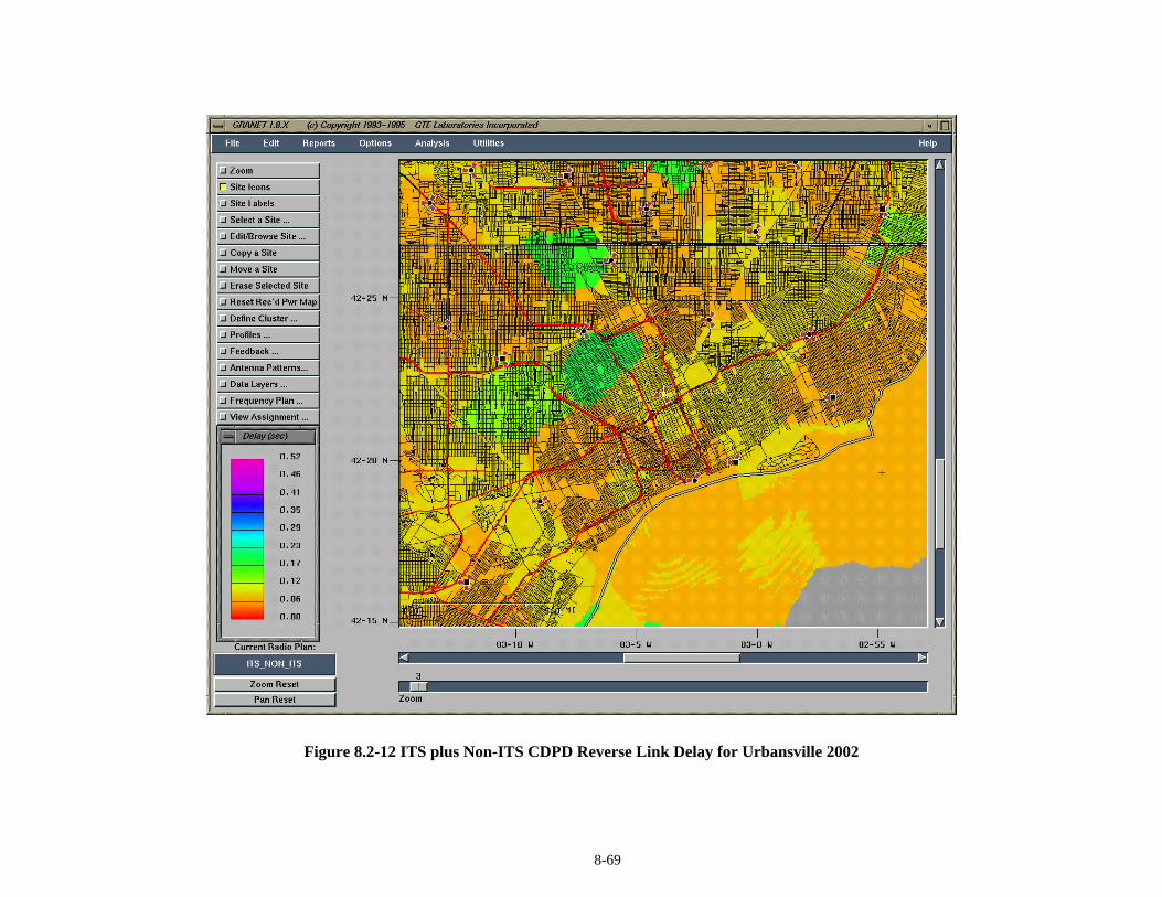
8-69
Figure 8.2-12 ITS plus Non-ITS CDPD Reverse Link Delay for Urbansville 2002

8-70
8.2.1.3.3 Peak-Period ITS plus Non-ITS with Incident
In Phase I, a worst case type incident was modeled but not specifically for Detroit. In Phase II, anaccident occurring in the CBD of the Detroit scenario was simulated with “incident loads” obtained fromMITRE from their vehicular traffic simulations.
We now analyze the impact of an incident on the CDPD performance. The average delay in the affectedsectors and in those in the immediate vicinity will be compared with those in absence of the incident. Forconvenience, the two sectors affected by the incident have been signaled in Figure 8.2-13 (gray instead ofblack) to make it easier to compare with the results in Figure 8.2-13 for the case of incident.
0
50
100
150
200
250
0 0.1 0.2 0.3 0.4
T hroughput (Erlang)
De
lay
(ms)
Figure 8.2-13 Delay-Throughput Pairs for Detroit 2002 for ITS plus Non-ITS in case of Incident
In the two sectors affected by the incident, the delay increased by a factor of 3.9% in the Tiger Stadium#1 sector, and by a factor of 7.95% in the Baltimore #3 sector. On the other hand, comparing the aboveresult with the one in absence of incident, we notice considerable fluctuation of the observed pairs, due toa natural statistical variation of the observed traffic from one simulation run to another. That fluctuationmakes the delay increase in the affected sectors almost meaningless (statistically insignificant). Again,the fact that we are in the “flat” portion of the curve makes the increase in delay due to the increase inload very small, and thus is buried in the statistical fluctuation.
Figure 8.2-14 presents a color-coded delay map of Detroit for the case of ITS plus non-ITS loads withincident affecting two of the downtown sectors.

8-71
Figure 8.2-14 ITS plus Non-ITS with Incident CDPD Reverse Link Delay for Urbansville 2002

8-72
8.2.1.4 Urbansville 2002 -- Dynamic Assignment of CDPD Channels (No Reserved Channel)
When the CDPD was initially conceived, the idea was to make exclusive use of the idle periods betweenvoice calls. In order to be able to do that, the MD-BS either has a connection to the Mobile SwitchingOffice (the AMPS switch), or has to implement “sniffing”, which is forward-sensing the channels that aremomentarily not in use.
A simpler method would be to reserve a channel for CDPD exclusive use, either by adding a new channelto the existing grouping, or by subtracting one from voice. The latter alternative is in general onlytemporary, since all cellular providers keep checking blocking probability, and adding channelswhenever it begins to approach the dreaded 2%.
The previous section looked into the performance of a system with a reserved CDPD channel in eachsector, the so called minimal CDPD deployment. Here we are going to analyze the case where no channelis reserved for CDPD, and only the idle periods are used.
Well established queuing theory results indicate that for a properly designed cellular network with areasonable number of channels per sector, which is always the case for urban environments, three CDPDchannels can capture, during the peak period, almost all the idle periods in the voice channels, and afourth would have minimal impact (very quickly diminishing returns). It should be noted that the cost ofthree CDPD channels per sector is considerably less than adding a new voice channel to each sector.
The performance of a 3-Dynamic CDPD channels (No Reserved) deployment will be assessed for the ITSplus non-ITS data Loads for the Detroit scenario. The resulting system performance is slightly better thanthat of the One Reserved CDPD channel minimal deployment.
8.2.1.4.1 System Performance for 3-Dynamically Assigned CDPD Channels
Figure 8.2-15 shows the delay PDF’s obtained for a totally dynamic deployment. The observed PDF’s arequite different from those obtained for one reserved CDPD channel. It is quite apparent the smallerstandard deviation of the delay that results from the availability of in general more than one channel forre-transmission in case of back-off due to collision or in case of packet error (remaining traffic hasalternative channels for delivery, and simultaneously is less likely to interfere with the re-trials).

8-73
0.10%
93.92%
1E-6
1E-5
1E-4
1E-3
1E-2
1E-1
1E+0
0 200 400 600 800 1000
Delay (ms)
PD
F
1 RS-block Long Packets
0.25%
93.34%
1E-6
1E-5
1E-4
1E-3
1E-2
1E-1
1E+0
0 200 400 600 800 1000
Delay (ms)
PD
F
2 RS-block Long Packets
Figure 8.2-15 Delay PDF’s as a Function of the Packet Length in RS-blocks, for 3-DynamicallyAssigned CDPD Channels (No Reserved) for ITS+Non-ITS Data Loads
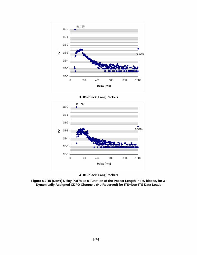
8-74
0.33%
91.36%
1E-6
1E-5
1E-4
1E-3
1E-2
1E-1
1E+0
0 200 400 600 800 1000
Delay (ms)
PD
F
3 RS-block Long Packets
0.34%
92.16%
1E-6
1E-5
1E-4
1E-3
1E-2
1E-1
1E+0
0 200 400 600 800 1000
Delay (ms)
PD
F
4 RS-block Long Packets
Figure 8.2-15 (Con’t) Delay PDF’s as a Function of the Packet Length in RS-blocks, for 3-Dynamically Assigned CDPD Channels (No Reserved) for ITS+Non-ITS Data Loads

8-75
0.42%
95.85%
1E-5
1E-4
1E-3
1E-2
1E-1
1E+0
0 200 400 600 800 1000
Delay (ms)
PD
F
5 RS-block Long Packets
Figure 8.2-15 (Con’t) Delay PDF’s as a Function of the Packet Length in RS-blocks, for 3-Dynamically Assigned CDPD Channels (No Reserved) for ITS+Non-ITS Data Loads
Figure 8.2-16 shows the behavior we came to expect. Also note the nearly perfect linear relation ofAverage Delay to Packet Length (driven by the channels fixed data rate).
0
20
40
60
80
100
120
140
1 2 3 4 5
Packet Length (RS-blocks)
Ave
rage
Del
ay/
Std
Dev
iatio
n (
ms)
Figure 8.2-16 Average Delay and Standard Deviation for 3-Dynamically Assigned CDPD Channels
Figure 8.2-17 shows the Delay-Throughput pairs for this totally dynamic deployment. The delay isobviously much smaller than in the case of One Reserved CDPD Channel, and the “curve” is now evenflatter.

8-76
0
20
40
60
80
100
120
140
160
180
0 0.1 0.2 0.3 0.4
Throughput (Erlang)
Del
ay (
ms)
Figure 8.2-17 Delay-Throughput for 3-Dynamically Assigned CDPD Channels (No Reserved) forITS+Non-ITS Data Loads
Since we had noticed fluctuations in the case of One Reserved channel, we looked at three distinct runsof the Dynamic Deployment for the Detroit scenario. The statistical fluctuations are here smaller (Figure8.2-18), reflecting the increased number of channels available on average for transmission.
0
50
100
150
200
250
0 0.1 0.2 0.3 0.4
Throughput (Erlang)
Del
ay (
ms)
Figure 8.2-18 Delay-Throughput Pairs Observed in Three Different Simulation Runs for 3-Dynamically Assigned CDPD Channels (No Reserved) for ITS+Non-ITS Data Loads
Figure 8.2-19 shows a color-coded delay map of Detroit for the case of ITS plus non-ITS loads for thisdynamic deployment.

8-77
Figure 8.2-19 CDPD Reverse Link Delay for ITS plus Non-ITS Data Loads and 3-Dynamically Assigned CDPD Channels

8-78
8.2.2 Thruville 2002
Coverage for the present cellular deployment, as well as best server information, (obtained usingGRANET), is shown in Figure 8.2-20.

8-79
Figure 8.2-20 Philadelphia-Trenton Corridor (Thruville) Coverage

8-80
For the data loads identified in Section 8.1.5, performance information was obtained for the casesof ITS Only, and ITS plus non-ITS. As in the previous cases for the Detroit cellular scenario, weobserve for the Philadelphia-Trenton cellular deployment, updated in March 1995, a few sectorsthat deviate from the expected Delay-Throughput curve.
Figure 8.2-21 shows that, for the small loads associated with ITS only, almost all sectors fall inthe “linear”, almost flat portion of the Delay-Throughput curve. Out of the 333 sectors in thescenario, only 13 have delays above 200 ms.
0
50
100
150
200
250
300
350
400
450
0 0.05 0.1 0.15 0.2 0.25 0.3 0.35
T hroughput (Er lang)
De
lay
(ms)
Figure 8.2-21 Delay-Throughput Pairs for ITS Only Data Loads for Thruville 2002
Figure 8.2-22 shows the performance of the system for ITS plus non-ITS Data Loads. Weobserve that almost all the Delay-Throughput curve is now filled. Exactly the same number ofsectors, 13, is now above 400 ms (two times 200 ms), when the reverse link load increased by afactor of 3.5.

8-81
0
100
200
300
400
500
600
700
0 0.2 0.4 0.6 0.8
T hroughput (Er lang)
De
lay
(ms)
Figure 8.2-22 Delay-Throughput Pairs for ITS plus Non-ITS Data Loads for Thruville 2002
As stated before, we had no opportunity to explore the effects of the incident “created” by theGovernment. However, comparing the Thruville incident scenario with that of Urbansville, wecan expect that the increase in data load due to the incident be, per cent-wise, even smaller in thiscase. This is in part because the incident expands over a much bigger region, and therefore ittakes that much longer to build the queues that were observed in MITRE’s simulation just beforethe incident began to clear. As a result, the increase in delay due to the (small) increase in loadwill, in all likelihood, be masked in the statistical fluctuation of the simulation.
8.2.3 Mountainville
Information on the cellular coverage in the Lincoln County, Montana area was used to computethe associated cellular coverage. A priori, full coverage of the area under consideration was notexpected – the relief and the low population density are such that only the major highways andpopulation concentrations have been targeted for coverage. However, looking at the obtainedcoverage information, we see that only a few deep valleys are not covered. The coverage forMountainville is shown in Figure 8.2-23.

Figure 8.2-23 Lincoln County, Montana (Mountainville) Coverage

8–83
8.3 Wireline System Performance
Simulations of wireline networks were performed in Phase I (see Phase I Document: Analysis ofData Loading Requirements). The results showed that for communication among ITS subsystemsthe delay of a reasonably designed network, with readily available technology, is extremely small(microseconds) and insignificant. Consequently, in Phase II the wireline simulation focused onthe wireline component of the CDPD network in order to obtain end-to-end system performance,including the effect of the higher layers of the protocol stack.
8.3.1 Traffic Over the Wireline Portion of the CDPD Network
Figure 8.3-1 shows the network to be simulated to assess the true end-to-end performance of theCDPD network. It takes into account all the CDPD traffic in the Urbansville area. It is based onthe cellular deployment information already collected (230 sectors in 80 sites), and essentiallyfollows the Rockwell Team’s Evaluatory design of Phase I: three jurisdictions; two MD-IS’sapproximately splitting the control of the sites; two TMS’s; and three (or possibly only two)ISP’s. One of the TMS’s, as well as one of the ISP’s see higher concentration of traffic since theycover the CBD of Detroit. Those will be therefore selected for the worst-case end-to-endperformance study.
In order to simplify the analysis, all users of a given type (of one of the groups identified above)will be treated as a composite source with the equivalent traffic. We will then identify the trafficthat originates and terminates at each mobile user group destined to and arriving from each of theF-ES’s of interest. In addition to the ISP, we have to consider the FMS, TRMS, EM, CVAS,PMS, and a few externals, like Pay Instrument, Location Data, and Intermodal FreightDepot/Shipper.

8–84
ISMD-IS
MDBS
IS
FMS
TRMS
ISP
RS
EM
“Internet”
FDDI
72
73
74
71
16 17
18
ISMD-IS
26 27
75
61
41 81
62
“2 DS0”
“112 DS0”
“115 DS0”
59
53
52
54
55
56
51
57
58 RAS
PIAS
VS
TRVS
CVS
EVS
RTS
FMSwl
CVCS
CVASPayInstrLocDataFrghtD PMSFrghtS
70 76 77 78 79 80
Figure 8.3-1 Network to be Simulated to Assess End-to-End Performance
Figure 8.3-2 shows the M-ES/F-ES Origin-Destination pairs of interest which will be simulated.Included are the non-ITS users (Remote Access - RAS) that also use the CDPD network toremotely access their home systems, mainly for the purpose of retrieving e-mail messages.
Figure 8.3-2 M-ES/F-ES Origin-Destination Pairs
Table 8.3-1 describes the traffic between ITS pairs, thus enabling an accurate simulation of theCDPD network performance in the Urbansville area.

8–85
Table 8.3-1 ITS Origin-Destination Pairs Traffic (RS-blocks/s/Sector)
<<<<Forward F1 F2 F3 F4 F5 Reverse>>>> R1 R2 R3 R4 R5CVCS CVAS 0.000 0.000 0.000 0.000 0.000 0.000 0.000FMS CVAS 0.003 0.001 0.002 0.000 0.004 0.002 0.002FMS EM 0.000 0.000 0.000 0.000 0.000 0.000FMS ImFrghtD 0.000 0.000 0.000 0.000FMS ImFrghtS 0.000 0.000 0.000 0.000FMS ISP 0.149 0.009 0.084 0.019 0.028 0.009 0.103 0.047 0.037 0.019FMS PayInstr 0.000 0.000 0.000 0.000PIAS EM 0.000 0.000 0.000 0.000PIAS ISP 0.032 0.002 0.000 0.020 0.006 0.003 0.006 0.000 0.002 0.004 0.000PIAS LocData 0.000 0.000PIAS PayInstr 0.000 0.000 0.000 0.000PIAS TRMS 0.001 0.001 0.000 0.000RTS EM 0.000 0.000RTS ISP 0.000 0.000 0.000 0.000 0.001 0.001 0.000 0.000 0.000RTS PayInstr 0.000 0.000 0.000 0.000 0.000CVS FMS 0.234 0.074 0.057 0.057 0.009 0.037 0.175 0.042 0.132 0.000EVS EM 0.018 0.012 0.006 0.029 0.023 0.006TRVS PayInstr 0.004 0.004 0.000 0.009 0.009TRVS TRMS 0.128 0.004 0.013 0.086 0.023 0.002 0.091 0.005 0.015 0.062 0.009VS EM 0.000 0.000 0.000 0.000 0.000VS ISP 0.210 0.095 0.092 0.024 0.000 0.045 0.006 0.037 0.002VS LocData 0.001 0.001VS PayInstr 0.000 0.000 0.000 0.000 0.000VS PMS 0.000 0.000 0.000RAS RS 6.513 3.473 1.380 1.026 0.414 0.220 1.897 0.938 0.507 0.293 0.117 0.042

8–86
8.4 End-to-End System Performance
8.4.1 Scope of Performance Analysis
The cellular simulation capabilities of GTE Laboratories (GTEL) are combined with Loral’sprotocol simulation capabilities to provide the end-to-end performance. GTEL’s MOSSaccurately characterizes the lower layers of the CDPD protocol (MAC and Physical in Figure8.4-1) in the reverse direction by using accurate propagation information obtained fromGRANET and by taking into account all the interference effects arising from both voice and data.Loral’s OPNET model of the CDPD protocol is used to model the higher layers, and the forwardlink, given that it operates in a broadcast mode (i.e., no contention).
Figure 8.4-1 shows the protocol stack to be simulated. The first observation is that for mostapplications, the Session, Presentation and Application layers are merged together. Thus, end-to-end performance will be measured from the moment information is delivered to the Transportlayer at the Mobile or Fixed End Systems (M-ES/F-ES) till the moment it is delivered by theTransport layer at the other end (F-ES/M-ES).
Transport
Network
DeviceDriver
DeviceDriver
MDLP
MAC
Physical
Network
DeviceDriver
M-ES CDPDModem
MDBS MD-IS IS F-ES
SNDCP
MDLP
MAC
Physical
Transport
Application
Presentation
Session
Serial(RS-232)
Application
Presentation
Session
RadioLink
SNDCP
MOSS
Figure 8.4-1 CDPD Protocol Stack for End-to-End Performance Evaluation (Shows thePortion to be Replaced by MOSS’ CDPD Traffic Characterization in Terms of Delay)
The scope of MOSS (and GRANET) is clearly identified in Figure 8.4-1. The delaycharacterization of the CDPD reverse link will be used to account for the over-the-air delay. As amatter of fact, the lower layers of the CDPD protocol guarantee delivery of information from theM-ES to the MD-BS. MOSS does in fact “listen” to the forward channel to make sure it accountsfor contention and other channel impairments as detected at the MD-BS.

8–87
With this integrated model (OPNET using the CDPD reverse channel characterization obtainedfrom MOSS and GRANET), the Joint Team obtained end-to-end (application to application)CDPD delay information, thus answering some of the questions raised at the conclusion of PhaseI. The performance of the CDPD networks deployed in Urbansville (based upon actual cellulardeployment in the areas that inspired those scenarios) during the peak period was used forarriving at the end-to-end delay.
8.4.2 Results
Simulation results are obtained for the important segments of the overall CDPD network –emphasizing non-ITS users, and the effect of the overall traffic in the CDPD network. See Figure8.4-2.
M-ES’s
* One DS0 line per CDPD channel
59
53
52
54
55
56
51
57
58
72
73
74
71
75
16 17
18
F-ES’s
ISMD-ISMDBS
RAS
PIAS
VS
TRVS
CVS
EVS
IS
FMS
TRMS
ISP
RS
EM
DS0 - T1
DS0
DS0
“Internet”
DS0
FDDI
ISMD-IS
DS0
DS0(’s)
*
RTS
FMSwl
CVCS
CVASPayInstrLocData
FrghtD
PMS
FrghtS
78 79 80 70
76 77
Figure 8.4-2 Portion of the CDPD Network that has been Simulated (Corresponding to OneSector of the Cellular Deployment)
The choice of specific links in the simulation (DS0 and T1) is determined by the expected trafficto and from the aggregated F-ES’s for the various service groupings.
Table 8.4-1 presents the cumulative traffic to and from the F-ES’s. It can be seen that, except forthe Emergency Management and Transit Management subsystems, which can do with a DS0 line(56 kbps capacity), all others need to have a higher capacity connection. In most cases, thishigher capacity will be achieved by leasing a few DS0 lines, allowing for flexibility in addingmore, whenever needed while paying only for the required throughput, instead of going directlyto fractional T1 or even T1 lines.

8–88
Table 8.4-1 Total Traffic Departing from/Arriving at the F-ES’s
1 SectorOrigin Dest <<<<Forward F1 F2 F3 F4 F5 Reverse>>>> R1 R2 R3 R4 R5
CVAS 0.003 0.001 0.002 0.000 0.004 0.000 0.002 0.002EM 0.018 0.012 0.000 0.006 0.029 0.023 0.000 0.006
FMS 0.234 0.074 0.057 0.057 0.009 0.037 0.175 0.042 0.132 0.000ImFrghtD 0.000 0.000 0.000 0.000ImFrghtS 0.000 0.000 0.000 0.000
ISP 0.391 0.011 0.179 0.131 0.058 0.013 0.155 0.047 0.046 0.041 0.020 0.000LocData 0.001 0.001PayInstr 0.005 0.005 0.000 0.009 0.009 0.000
PMS 0.000 0.000 0.000RS 6.513 3.473 1.380 1.026 0.414 0.220 1.897 0.938 0.507 0.293 0.117 0.042
TRMS 0.129 0.004 0.014 0.086 0.023 0.002 0.091 0.005 0.015 0.062 0.009
2 Sector Load<<<<Forward F1 F2 F3 F4 F5 Reverse>>>> R1 R2 R3 R4 R5
#62 CVAS 0.006 0.001 0.004 0.001 0.007 0.000 0.003 0.004#62 EM 0.035 0.023 0.000 0.012 0.059 0.047 0.000 0.012#62 FMS 0.468 0.148 0.114 0.113 0.019 0.074 0.349 0.085 0.264 0.001#62 ImFrghtD 0.001 0.001 0.001 0.001#62 ImFrghtS 0.001 0.001 0.001 0.001#62 ISP 0.782 0.022 0.357 0.262 0.116 0.025 0.309 0.094 0.092 0.082 0.041 0.000#62 LocData 0.003 0.003#62 PayInstr 0.010 0.010 0.000 0.019 0.019 0.000#62 PMS 0.000 0.000 0.000#62 RS 13.025 6.946 2.761 2.051 0.828 0.441 3.793 1.876 1.014 0.585 0.234 0.085#62 TRMS 0.258 0.007 0.028 0.173 0.047 0.004 0.183 0.011 0.030 0.124 0.017
112 Sector Load<<<<Forward F1 F2 F3 F4 F5 Reverse>>>> R1 R2 R3 R4 R5
#61 CVAS 0.330 0.072 0.221 0.036 0.410 0.001 0.181 0.228#61 EM 1.972 1.312 0.004 0.656 3.295 2.630 0.009 0.656#61 FMS 26.195 8.293 6.364 6.346 1.046 4.147 19.561 4.759 14.765 0.036#61 ImFrghtD 0.054 0.054 0.054 0.054#61 ImFrghtS 0.054 0.054 0.054 0.054#61 ISP 43.818 1.243 20.012 14.668 6.473 1.422 17.308 5.248 5.153 4.594 2.293 0.020#61 LocData 0.152 0.152#61 PayInstr 0.564 0.540 0.024 1.060 1.060 0.000#61 PMS 0.004 0.002 0.002#61 RS 729.421 388.954 154.590 114.858 46.344 24.675 212.431 105.030 56.772 32.769 13.118 4.741#61 TRMS 14.439 0.397 1.543 9.663 2.615 0.222 10.223 0.595 1.685 6.965 0.979
115 Sector Load 20% goes to the F-ES's of the other region
<<<<Forward F1 F2 F3 F4 F5 Reverse>>>> R1 R2 R3 R4 R5#41 CVAS 0.068 0.015 0.045 0.007 0.084 0.000 0.037 0.047#41 EM 0.405 0.269 0.001 0.135 0.677 0.540 0.002 0.135#41 FMS 5.379 1.703 1.307 1.303 0.215 0.852 4.017 0.977 3.032 0.007#41 ImFrghtD 0.011 0.011 0.011 0.011#41 ImFrghtS 0.011 0.011 0.011 0.011#41 ISP 8.998 0.255 4.110 3.012 1.329 0.292 3.554 1.078 1.058 0.943 0.471 0.004#41 LocData 0.031 0.031#41 PayInstr 0.116 0.111 0.005 0.218 0.218 0.000#41 PMS 0.001 0.000 0.000#41 RS 149.792 79.875 31.746 23.587 9.517 5.067 43.624 21.569 11.659 6.729 2.694 0.974#41 TRMS 2.965 0.082 0.317 1.984 0.537 0.046 2.099 0.122 0.346 1.430 0.201
#41 #81 671.107 328.735 150.549 119.749 47.049 25.025 217.186 94.984 67.413 36.598 14.280 3.911

8–89
Preliminary simulation results are available and they are presented below for some of the O-Dpairs previously identified. We account separately for the traffic in both directions. The mainjustification for this approach, besides the resulting simplification of the simulation effort, is thatas stated at the outset, we are only taking into account the communication delay, and not the ITSSubsystems performance. The overall end-to-end delay can thus be approximated by adding tothe independent delays in both directions, and then providing a margin for the expectedprocessing and information access times at the F-ES’s.
Figures 8.4-3 to 8.4-7 show the delay in both directions for the most relevant M-ES/F-ES O-Dpairs: Private Vehicle-ISP, CVO Local-FMS, and RAS-RS, assuming an initial period of 100 swith no packet loss followed by 40 s of 10% packet loss and then 60 s again with no packetloss. Lost packets will eventually be retransmitted, as soon as the TCP timers at either endexpire. This implies necessarily an increase in the overall CDPD traffic. As a firstapproximation, we can assume that there is a resulting 10% increase in the traffic in bothdirections between RAS and RS. Due to time and resource constraints, it was not possible torecompute the reverse link CDPD delay for this higher traffic, so the same CDPD delaydistribution was used over the whole observation period. From all the analysis in Section 8.1 and8.2, we are confident that the increase in delay due to this additional traffic would be minimal,since we are operating in a lightly loaded network.
Figure 8.4-3 shows the delay for the link directly affected by the packet loss. The increase indelay due to retransmission is obvious. However, the effect of the increase in traffic shows up onthe other links: Figures 8.4-4 to 8.4-7 not only show a slight increase in delay, but hint at a slowrecovery of the network.
In any case, the reverse link (including the CDPD Reverse Link) has higher delays, as expected,due to the contention mechanism involved.
In all cases, the delay is still quite small, less than 2 seconds, which is well within the delayrequirements of the various ITS services employing wide area wireless/wireline informationexchange.

8–90
0
0.2
0.4
0.6
0.8
1
1.2
1.4
1.6
1.8
0 50 100 150 200
T ime (s )
Reve
rse
Dire
ctio
n D
ela
y (s
)
Figure 8.4-3 RAS -> RS (Reverse Link) Assuming 100 s with No Packet Loss followed by 40s with 10% Packet Loss, and then 60 s with No Packet Loss

8–91
0
0.02
0.04
0.06
0.08
0.1
0.12
0.14
0.16
0.18
0 50 100 150 200
T ime (s )
Forw
ard
Dire
ctio
n D
ela
y (s
)
Figure 8.4-4 FMS -> CVO Local (Forward Link)
0
0.05
0.1
0.15
0.2
0.25
0.3
0 50 100 150 200
T ime (s )
Reve
rse
Dire
ctio
n D
ela
y (s
)
Figure 8.4-5 CVO Local -> FMS (Reverse Link)

8–92
0
0.02
0.04
0.06
0.08
0.1
0.12
0.14
0.16
0.18
0.2
0 50 100 150 200
T ime (s )
Forw
ard
Dire
ctio
n D
ela
y (s
)
Figure 8.4-6 ISP -> Private Vehicle (Forward Link)
0
0.05
0.1
0.15
0.2
0.25
0 50 100 150 200
T ime (s )
Reve
rse
Dire
ctio
n D
ela
y (s
)
Figure 8.4-7 Private Vehicle -> ISP (Reverse Link)

9-1
9. ITS ARCHITECTURE COMMUNICATION – CONCLUSIONS
In the last decade, many communication technologies and systems have been introduced at anever-accelerating pace, and some are gaining wide acceptance. The complex world oftelecommunications is evolving and expanding rapidly. For many application areas, includingtransportation, myriad communication options are available to the system architect and designer.These solutions, of course, meet the requirements at hand with varying degrees of satisfaction,with implications of performance, cost, and user acceptance.
The ITS world is broad and varied, as amply demonstrated by the twenty nine ITS user serviceswith their distinct needs and complex interactions. The National ITS Architecture can be viewedas a framework that ties together the transportation and telecommunication worlds to enable thecreation, and effective delivery, of the broad spectrum of ITS services. Throughout theArchitecture effort, the emphasis has been on flexibility. This aims to allow the localimplementors and service providers to select the specific technologies, within the framework ofthe architecture, that best meet their needs (expressed either in terms of market realities orjurisdictional constraints).
A basic architectural concept espoused in the definition of the National Architecture is that of aPhysical Architecture with a Transportation Layer and a Communication Layer. This concept isspecifically intended to mitigate the complexity that arises from the flexibility sought in the ITSArchitecture. It enables the separation of the two fairly independent domains of transportationand communication, yet, at the same time, maintaining them tightly coupled to meet the ITSusers service requirements. Through this framework, the interconnectivity requirements betweenthe transportation systems can be derived from the ITS user services, and various communicationchoices can be considered, and objectively evaluated, for their ability to meet those connectivityrequirements.
This National ITS Communication Document has presented, under the same cover, theinformation necessary to describe and characterize all aspects of communications within theNational ITS Architecture. The first ingredient provided is a thorough, coherent definition of the“communication layer” of the Architecture.

9-2
The Communication Layer (or architecture) for ITS has two components: one wireless and onewireline. All Transportation Layer entities requiring information transfer are supported by one orboth of these components. In many cases, the communication layer appears to the ITS user (onthe transportation layer) as “communication plumbing”, many details of which can, and should,remain transparent. Nevertheless, the basic telecommunication media types have criticalarchitectural importance. The wireline portion of the network can be manifested in manydifferent ways, most implementation dependent. The wireless portion has three basic and distinctmanifestations:
• Wide-area wireless infrastructure, supporting wide-area information transfer (many dataflows). For example, the direct use of existing and emerging mobile wireless systems. Thewireless interface to this infrastructure is referred to as u1. It denotes a wide area wirelessairlink, with one of a set of base stations providing connections to mobile or untetheredusers. It is typified by the current cellular telephone and data networks or the larger cells ofSpecialized Mobile Radio for two way communication, as well as paging and broadcastsystems. A further subdivision of this interface is possible and is used here in the document:u1t denotes two-way interconnectivity; and u1b denotes one-way, broadcast-typeconnectivity.
• Short range wireless infrastructure for short-range information transfer (also many dataflows, but limited to specific applications). This infrastructure would typically be dedicatedto ITS uses. The wireless interface to this infrastructure is referred to as u2, denoting a short-range airlink used for close-proximity (typically less than 50–100 feet) transmissionsbetween a mobile user and a base station, typified by transfers of vehicle identificationnumbers at toll booths.
• Dedicated wireless system handling high data rate, low probability of error, fairly shortrange, Advanced Highway Systems related (AHS-related) data flows, such as vehicle tovehicle communication systems. This wireless interface is denoted by u3. Systems in thisarea are still in the early research phase.
The ITS network reference model was tied to the specific interconnections between thetransportation subsystem, e.g., connection between Information Service Provider (ISP) subsystemand a vehicle subsystem (VS) through the Architecture Interconnect Diagram (AID), actually, awhole collection of them of varying levels of detail. The Level-0 AID provided is the top leveldiagram showing the types of interconnectivities between the various transportation subsystems.It is, perhaps, the best description of the communication framework in the ITS architecture. ThisAID Level-0 was broken down further to show subsets of it depicting certain interconnectivitiesof interest, for example, in one case the data flows which use broadcast (u1b), and in another,those that use either broadcast (u1b) or two-way wide area wireless (u1t).
Various media and media types are applicable as possible candidates for each type ofinterconnection. The best communication technology family applicable to each data flow wasspecified. This remained above the level of identifying a specific technology or system. Inpractice, i.e., in a real-world ITS deployment, the final step of selecting a given technologywould be performed by the local ITS implementor or service provider. A detailed specificationhere would have clearly crossed the boundary of architecture definition into the realm of systemdesign.
To assist the implementors and service providers in the ITS community, a broad and balancedtechnology assessment was performed. It used as much factual information as was publiclyavailable to identify and compare key pertinent attributes of the different communicationtechnologies from a National ITS perspective.

9-3
A host of land-mobile (i.e., cellular, SMR, paging, etc.), FM broadcast, satellite, and short rangecommunication systems have been assessed. The assessment addressed the maturity of thecandidate technologies and analyzed their capability for supporting ITS in general, and thearchitecture in particular. Within the limits of reliable, publicly available information, thefollowing attributes were assessed: infrastructure and/or service cost as applicable, terminal cost,coverage, and deployment time-line (if not yet deployed). Furthermore, interface issues (i.e.,open versus proprietary) were also addressed from a national ITS perspective. Wheneverpossible, analysis was performed to determine among other things : 1) supported data rate, 2)delay-throughput, 3) mobility constraints, etc. The ITS Architecture data flow specificationswere used in the analysis, including message sizes and update frequencies whenever appropriate.The key comparison characteristics were finally summarized in tables.
Some of the broad conclusions of this assessment are listed below:
A large set of architecture data flows, basically the vast majority of the u1t flows, are bestsupported by commercially available mobile wireless data networks, operated in the packetswitching mode. Prominent among these today are CDPD, and private packet radio networksystems like RAM and ARDIS. Like the rest of wireless communication, the field is expandingand new candidate systems are joining the arena.
CDPD’s technical performance has been validated through ITS-related simulation, as describedin Section 8, and through operational field trials (as in the example provided in Appendix J).CDPD is promising because it may provide coverage over the entire footprint of the cellularsystem in a few years. At the end of 1995, 42% of the population was covered. It is projected that75% of the population would be covered before the end of 1997. Another version of CDPD,which extends IP capabilities to regular AMPS cellular channels and to the PSTN is called“Circuit Switched CDPD”, and will be used to extend CDPD service to areas that do not have thefull CDPD overlay implementation on the cellular base stations. Nevertheless, some areas maynever have CDPD in any form, and may transition directly to other, more advanced, cellular- orPCS-based packet data systems. (The little information available on those very new systems hasbeen included in the technology assessment sections.)
Service prices for CDPD have gone down to where a mass market can develop, if equipmentcosts were to drop to the $200 range, and more applications became available. This will takesome time, i.e., a few years, and ITS is no different in this aspect than other wireless dataapplication areas. ITS applications will benefit from the developments, and users acceptancetrends, in the broader fields of the mobile office and wireless Internet access.
RAM and ARDIS both have nation-wide coverage that is focused on major metropolitan areas,where there is significant business activity. Since they are basically proprietary systems, it ishard to draw conclusions on their performance (delay/throughput, capacity, and so on). However,anecdotal evidence indicates that they may perform adequately for ITS applications. Non-opensystems are generally perceived to be less cost advantageous to the user than open systems. Asfar as the ITS consumer is concerned, if no cost penalty is perceived, the customer may wellchoose one of these solutions if the ITS service provider offers the service through them. Issuesof coverage outside metropolitan areas, and national inter-operability, may or may not be ofconcern to the end user. Final decisions on which medium to select will rest with the end usersand their constraints, and will be heavily influenced by cost.
Metropolitan area network (MAN) type wireless data systems intended for the non mobile user(only for fixed and pedestrian speeds), such as systems by Metricom and TAL, can be used forITS information access, or other ITS user services if the user’s mode of utilization is not mobileand the application is not time critical. These systems could offer price advantages over mobile

9-4
wireless data systems, because of simplicity. Prices of wireless data services will all follow adownward trend. However, individual prices for specific uses are harder to predict than theweather! The economic tradeoffs would obviously have to be performed by the consumer on acase by case basis.
Two way paging (narrow band PCS) systems were also assessed. These can be used to carry ITSservices that are not time critical, or that do not require a real time response. Particularly suitablewould be messages for which a canned response would suffice. Whether these features would beacceptable or not to an end customer, is a function of the detailed implementation of the ITSapplication offered by the service provider.
An array of satellite systems was also assessed for supporting the National ITS Architecture.These include a variety of Little (data only) and Big (voice and data) low-earth-orbit (LEO)systems, as well as more conventional medium-earth-orbit (MEO) and geosynchronous (GEO)satellite systems. Most of these systems are not yet deployed but are projected to be in service ina few years. Because of terminal and service cost, satellite systems in general would be usedwhere terrestrial alternatives (e.g., those listed above) are not available. Little LEO choices seemto be the most appropriate for ITS among satellite systems, since they are targeted specifically toshort bursty data transactions.
As for one way ITS data flows, those can be carried on one of several Broadcast media. The mostprominent among these are FM Subcarrier systems. A detailed quantitative assessment of thethree leading high speed subcarrier systems was performed. These are the HSDS, DARC, andSTIC systems, which all have roughly 7-8 kbps throughput. The analysis showed that any wouldbe adequate to carry the broadcast data flows envisioned and incorporated into the definition ofthe architecture. Cost and reliability of the communication service will depend on the details ofthe infrastructure deployment and the implementation of the service. At this point, those systemsare vying for a share of the market and for becoming a national standard. The low speed RBDSFM subcarrier standard can also be used for the ITS data flows if the update rates are maintainedlow, at about once per ten minutes, again depending on the detailed implementation of theservice.
It should be kept in mind that broadcast links, those denoted u1b, do not have to be implementedover FM subcarrier. Many two-way wireless systems, such as two-way paging and CDPD, havebroadcast protocols in the forward direction (infrastructure to vehicle), and could, in principle, beused. Also any array of one-way paging services could be used in one form or another. The costof service and equipment, and the detailed service features, will determine the approach mostattractive to customers and ITS service providers.
One of the great advantages of the wide-area wireless, u1, interface defined in thecommunication layer of the National ITS Architecture, is that it relies on sharing ofcommercially available wireless infrastructures. Over the next several years, an explosion of suchwireless infrastructures and services will be taking place. ITS will stand to benefit enormouslyfrom this powerful trend, and must leverage it to the fullest extent.
The second distinct type of infrastructure required in the ITS architecture is for dedicated shortrange communication (DSRC). This utilizes the so-called beacon systems, which are typically RFtransponders mounted in very close proximity to the road infrastructure. Because of theirdedicated nature, which implies that all their costs have to be absorbed by the ITS applicationsthey support, as well as their limited range, these systems must be used judiciously. They areadopted in the ITS Architecture only for specific ITS user services whose implementationrequires the close physical proximity that wide area wireless systems cannot achieve, eithertechnically or cost-effectively. For example, they are used for toll collection, CVO credentials

9-5
checks, parking lot management, and the like. There are some services that could be supported byeither the DSRC or wide area wireless, such as fixed-route transit support. For those, thearchitecture allows for flexibility, and local implementors would need to perform the pertinentcost tradeoffs. For some services, such as vehicle probes, the DSRC, where available for otheruses, can be utilized to complement wide area wireless and wired physical sensor systems.
One of the salient conclusions of the Architecture exercise is that short range beacon systemsshould not be used as a replacement of wide-area wireless systems. In other words, they shouldnot be used to carry such ITS user services as route guidance, mayday, commercial fleetmanagement (dispatch), and so on. The rationale is both technical and economic, and isdiscussed in the main text and supporting appendices of this document. Basically, beaconsystems are not suitable for time critical wide area services, or for those that cannot tolerateinterruptions of coverage. However, the cost of widespread urban deployments of such shortrange systems (e.g., 18,000 beacons to cover 11% of the roads in metro Detroit) would simply beprohibitive and unjustifiable.
There are at present several DSRC technologies, mostly using RF transponders. Some usepassive and others active vehicle transponders (tags). In the applications or deployments whereone transponder per lane is used , there is no technical basis for selecting one class over theother. In applications where a single beacon is to cover multiple lanes, active vehicletransponders can offer superior performance. There are also beacon systems that operate in theinfra-red spectrum; their role is harder to predict at this point. In any event, the ITS architectureshould start by accommodating multiple technologies, and gradually transition to the adoption ofa single standard that would facilitate the national inter-operability of all the DSRC applications.
From a National ITS Program perspective, the architecture development effort encompassed twobroad thrusts: (1) communication architecture definition, i.e., selection of communication serviceand media types to interconnect the appropriate transportation systems, and (2) several types ofinter-related communication analyses, to ensure the feasibility, and soundness, of thearchitectural decisions made in the definition. The two major communication analysis areas havebeen:
• An analysis of the data loading requirements derived from the ITS service requirements, theLogical and Physical Architectures and their data flows, the ITS service deploymenttimeline, and the attributes of the candidate scenarios in the “evaluatory design”.
• An in-depth, quantitative analysis of the real-world performance of selected technologies thatare good candidates for adoption as ITS service delivery media, and for which reliable, state-of-the-art simulation tools are available. The performance is determined under the demandsof the ITS and other projected applications of the media.
The overall objective of the analyses has been to ascertain whether the National ITS Architectureis feasible from the standpoint that communication technologies exist and will continue to evolveto meet its demands, both technically and cost-effectively. To set the stage for this, data loadinganalyses were completed for the wide area wireless interfaces u1t, u1b, and the wireline interfacew – data loading for the u2 and u3 interfaces is not as useful, so link data rates were determinedinstead.
The data loading analysis has defined all of the messages that flow between the transportationsubsystems. Deployment information from the evolutionary deployment strategy was used todefine which services, and therefore which messages would be available for each of the scenarioand time frames specified by the Government. The three scenarios provided were addressed,

9-6
namely, Urbansville (based on Detroit), Thruville (an inter-urban corridor in NJ/PA), andMountainville (a rugged rural setting based on Lincoln County, Montana).
Seven user service groups with distinct usage patterns were defined, along with the frequency ofuse of the messages by each user group. Messages were assigned to the u1t, u1b, and winterfaces based on suitability, and were allowed to flow over multiple interfaces with a fractionassigned to each one. The resulting data loading analyses provided the data loads on all of theabove interfaces and links, and a complete description of the message statistics, which were usedto drive the communications simulations.
For the u1t interface, the data loading results indicate that for Urbansville in 2002 the largest dataloads would result from the CVO-local user service group, followed closely by transit and privatevehicles. In Thruville, for the same time period, CVO-local and transit would be the largest datausers. For Urbansville in 2012, private vehicle and CVO-local would be the largest data users, atabout twice the rate of transit, with the others far below. For Thruville in 2012, CVO-localremains the largest data user, followed by transit. The Mountainville data loads are very low,with CVO-local the largest user, followed by private vehicles.
The ITS Architecture data loading information was used as input to the communicationsimulations. Due to the relative scarcity of wireless resources (relative to wireline) emphasis wasplaced on the evaluation of wireless system performance. However, network end-to-endperformance, comprising both the wireless and wireline components, given in terms of delay andthroughput was also obtained. Furthermore, representative analyses of a wireline networks havealso been included.
The wireless simulations performed were for Cellular Digital Packet Data (CDPD), primarilybecause it is an open standard with a publicly available specification, and because validated,state-of-the-art simulations were made available for use on the ITS Architecture Program. Thesesimulations accurately reflect the mobile system conditions experienced in the real world,including variable propagation conditions, land use/land cover information, user profiles, andinterference due to other (voice and data) users. These modeling tools have been tested in thedeployment and engineering of commercial wireless networks by GTE.
Simulations have been run for two of the three scenarios provided by the Government only forthe 2002 time frame, not only due to the lack of time to analyze all time frames, but because 10years is the farthest one can accept using present day deployment information. Since the numberof users is very small in Mountainville, only cellular coverage was obtained to ascertain itsadequacy in that remote area. For both Urbansville and Thruville, scenarios with both ITS andNon-ITS data traffic projected for the CDPD network were run, under normal peak conditionsand in the presence of a major incident.
The Government-provided scenario information was substantially augmented with informationon actual cellular system deployment obtained directly from FCC filings. A minor amount ofradio engineering was performed to fill a few gaps in the information obtained, especially for theThruville scenario. The commercial wireless deployment assumed in the simulation runs,therefore, was representative of the real operational systems. In fact, because of the continuousand rapid expansion of these systems, the results of the simulations should be viewed as worstcase in nature.
The wireless simulation results have shown that the reverse link delay, even in the presence ofnon-ITS data, and in the case of an incident during the peak period, is very low (150 ms for ITSonly; 300 ms for ITS plus non-ITS; with a 10% increase in the cell sectors affected by theincident).

9-7
The results of the CDPD simulations have further been validated by the results of an operationalfield trial that was performed in the spring of 1995, jointly by GTE and Rockwell, in the SanFrancisco Bay Area. The application demonstrated was commercial fleet management, usingGPS location, and CDPD as an operational commercial wireless network. A synopsis of the trialand its results have been presented in Appendix J.
The results for CDPD, summarized above, should be interpreted as a “proof by example”. Acommercial wireless data network is available today to meet the projected ITS requirements.Other networks also exist, and can be used, as indicated in the technology assessment sections.Future wireless data networks will be even more capable.
As for broadcast systems, the quantitative analysis has shown that the combination of the low-rate RDBS with the emerging high data rate FM subcarrier standard will satisfy the ITSArchitecture broadcast requirements in the foreseeable future. New broadcast techniques,including Digital Audio Broadcasting, which is on the horizon, will accommodate any long termgrowth.
The simulation results for the wireline network example deployment indicate that extremelysmall and completely insignificant delays are encountered, when the system is designed to beadequate for the projected use. With the capacities achievable today with fiber, whether leased orowned, wireline performance adequacy is not really an issue. The key issues there pertain to thecosts of installation and sustained operation for any given ITS deployment scenario.
The overarching conclusion from the data loading and communication system performanceanalyses is that commercially available wide area wireless (including broadcast) and wirelineinfrastructures and services adequately meet the requirements of the ITS architecture in thoseareas. These systems easily meet the projected ITS data loads into the foreseeable future, andthrough natural market pull, their continued expansion will meet any future ITS growth. Hence,from that particular standpoint, the National ITS Architecture is indeed sound and feasible.

Communications Document Addendum
January 1997i
TABLE OF CONTENTS
1. INTRODUCTION 1
1.1 Background 1
1.2 Relationship to other Documents 1
1.3 Organization of this Addendum 2
2. HRI PHYSICAL ARCHITECTURE 2
3. COMMUNICATIONS ARCHITECTURE SUPPORT FOR HRI 5
3.1 Approach 5
3.2 HRI-Specific Communications Architecture Elements 63.2.1 HRI Data Flow Mapping 63.2.2 HRI Architecture Interconnect Diagram 8
4. HRI DATA LOADING ANALYSIS 9
4.1 Approach 9
4.2 Source Data 9
4.3 Assessment 9
5. COMMUNICATION TECHNOLOGIES REVIEW 13
5.1 Wireline Communications 145.1.1 Candidate Wireline Technologies 145.1.2 Candidate Wireline Topologies 165.1.3 Public Network Usage 165.1.4 Localized Use of Internet 17

Communications Document Addendum
January 19971
1. INTRODUCTION
1.1 Background
The initial development of the National Intelligent Transportation System (ITS) Architecture wascompleted in July 1996. Leading up to this milestone was an intensive 33 month effort consistingof two phases and involving broad participation by public sector, industry, and academicstakeholders. The end-result of this effort was a single national ITS architecture which reflects thisbroad consensus input. This baseline architecture provides a structure through which the 29 ITSuser services identified in the National Program Plan can be delivered throughout the United States.The architecture and analyses presented in the separate Communications Document deliverablewere developed to support the original 29 user services.
More recently, a 30th user service has been developed that identifies the needs for Highway-RailIntersections (HRI) under the guidance of the Federal Railroad Administration (FRA) and the USDOT ITS Joint Program Office (JPO). The JPO tasked the two architecture teams, headed byRockwell International and Lockheed Martin, to modify the national architecture to include thisnew user service. This addendum provides a review and focused presentation of the elements ofthe communications architecture and communications analyses which apply to this additional userservice.
1.2 Relationship to other Documents
This Communications Document addendum is one of a series of reports documenting the NationalITS Architecture. In general, sufficient background information has been provided within thisaddendum so that it may be used without reference to the other reports. The interested reader mayrefer to these additional reports for more comprehensive treatment of the elements of the overallnational architecture documentation that provide a context for this report. Several of the reportsthat are most pertinent to the subject matter of this document are briefly described in the followingparagraphs.
The Logical Architecture provides a functional view of all user services, including the HRI userservice. It defines the functions that support each user service and all of the information flows thatconnect these functions. The information flows are source requirements for the communicationsarchitecture that is defined in this addendum. The Logical Architecture consists of three volumesthat include diagrams that identify all functions and relationships, process specifications that definethe functional requirements in detail, and a data dictionary that fully defines all of the informationflows.
The Physical Architecture collects related logical architecture functions together into subsystems.It defines a set of architecture flows that show all of the data that passes between the subsystemsand the special characteristics and constraints associated with each interface. This definition ofsubsystem connectivity is the basis for the communications architecture.
The Communications Document presents a thorough analysis of the communications elements ofthe National Architecture that support 29 user services. Beginning with the communicationsrequirements associated with the architecture flows, data loading analysis, communicationstechnology surveys, and a detailed simulation of one candidate wireless communications

Communications Document Addendum
January 19972
technology is provided. This addendum extends the communications document by focusing on theimpacts to the communication architecture and communication analysis associated with the HRIuser service.
1.3 Organization of this Addendum
This addendum consists of five major sections that define the communications architecture thatsupports the HRI user service and provides selected communications analyses related to this userservice.
Following this introduction, section 2 provides a focused presentation of the elements of thephysical architecture that support the HRI user service. This is the one place in the NationalArchitecture documentation that provides such a focused treatment of the architecture definition forHRI with some supporting information regarding its derivation.
Section 3 maps the HRI architecture definition to an updated communications architecture. Allarchitecture flows which were defined to support HRI are mapped to this updated communicationsarchitecture. Only the elements of the communications architecture that were updated to supportHRI are presented. Refer to the Communications Document for a comprehensive treatment of theentire Communications Architecture.
Section 4 provides a qualitative assessment of the data loading requirements imposed by the HRIuser service. This assessment is based on the information flows defined in the logical architecturecoupled with an evaluatory design and implementation scenario that is consistent with those usedas a basis for the companion Cost Analysis Addendum that is published under separate cover.
Section 5 provides a brief review of some of the communications technologies that will supportHRI. This section is an excerpt of a more comprehensive technology assessment section that isincluded in the Communications Document.
2. HRI PHYSICAL ARCHITECTUREThe National ITS Architecture is composed of separate Transportation Layer and CommunicationLayer domains. The Transportation Layer elements involved in the HRI user service include fieldequipment at the highway-rail intersection, the management center equipment that operates andmonitors the field equipment, and the trains and highway vehicles that are managed by the HRIUser Service. The architectural requirements for these transportation elements are documentedunder separate cover in the Physical Architecture document. The communications layer identifiesthe general framework for interconnecting the Transportation Layer elements and also includessupporting communications technology and data loading implications for the user services. Thecommunication layer elements for the HRI user service is the focus for this addendum. In order toprovide context for the communications discussion, an overview of the overall architecture for HRIis provided in this section.
Figure 1 is a high-level depiction of the transportation elements required for the HRI user serviceand their general connectivity. It shows equipment and interfaces traditionally operated by therailroads as well as equipment under the jurisdiction of state and local transportation agencies andkey interfaces between highway and railroad assets that may be implemented to support HRIimprovements. Table 1 expands on the figure by providing a brief overview of each of theinterconnections.

Communications Document Addendum
January 19973
TRAINAPPROACHING
WaysideEquipment
IntelligentController
AutomaticGates/Barriers
TrafficSignals
VariableMessage Signs
Surveillance
Short RangeCommunications
Rail Operations Traffic Management
TrackCircuits
2
1
3
4
3 7
5
6
7
7
78
9
10
Figure 1: HRI Elements and Interconnects
Table 1: HRI Interconnects Overview
Type Purpose Variations
1 Physical Detect train presence, speed, acceleration Track circuits are the most commonmechanism; other technologies may alsobe applied.
2 WirelineDiscrete
Fail-safe discrete representation of trainactivity at the intersection
Characteristics will be a function of thesurveillance technology and waysideequipment requirements.
3 WirelineDiscrete
Fail-safe discrete activation ofsignals/gates at the grade crossing
Railroad grade crossing devices are 12volt systems. Highway-highwayintersection devices are 110 volt systems.
4 WirelineDiscreteor Data
Communicate train presence from waysideequipment that is aware of train activity toroadside equipment that manages highwaytraffic. The purpose today is to allowcontrol strategies at adjacent highway-highway intersections to adapt to HRIclosures. The same interface could beused to notify roadside equipment toactivate signals/gates and other trafficmanagement devices at the grade crossingin other implementations.
Several variations may be implementedin different scenarios and timeframes.Near term implementations pass adiscrete signal indicating that the gradecrossing is closed (“Interconnect”) orwarning that the crossing will be closedin a short time (“Preemption”). Thisbasic connectivity may be expanded to adata interface providing more detailedinformation on expected closure times,duration, and train activity.

Communications Document Addendum
January 19974
Type Purpose Variations
5 WirelineData
Monitoring and control of waysideequipment. Represents the railroadswireline network providing connectivity towireless base stations, switches, signals,gates and other networked railroad assets.
Network characteristics will be differentfor different railroads.
6 WirelessData
Communications with the train is analternative method for monitoring trainposition/speed and deriving HRI closurerequirements. Communications to thetrain enables early warning of potentialintersection hazards.
Communications from the train back to acontrol center (Rail Operations) prior toHRI activation vs. Short rangecommunications to wayside equipmentwhich locally determines HRI closurerequirements.
7 WirelineDiscreteor Data
Local monitoring and control of trafficsurveillance and traffic control devicesenabling monitoring and management ofhighway traffic in the vicinity of HRIs.
Intelligent devices require data interfacesto support programming and statusmonitoring. Basic signals require onlydiscrete voltage inputs.
8 WirelessData
Direct provision of HRI status data to in-vehicle devices. Data may be provided asinformational displays to the driver, usedto provide safety warnings to the driver, orused as an input to vehicle controlsystems.
Content and timing requirements for theinterface vary with intended in-vehicleapplication.
9 WirelineData
Central monitoring and control ofhighway traffic surveillance and controldevices.
Many different protocols currentlyimplemented. Potentially significantfuture migration to NTCIP as a standardfor this interface.
10 WirelineData
Sharing of HRI status and closureschedules between highway managementand rail management systems
Shared data may be limited to as-neededcommunication of detected equipmentfailures affecting HRI communications orextended to more regular communicationof real-time information enabling HRIclosure forecasts.
Figure 2 identifies the mapping between the HRI elements and the Physical Architecturesubsystems and interconnects. As can be seen, the physical architecture aggregates roadsidesurveillance, controller, and device equipment associated with HRI into the roadway subsystem.This approach is consistent with the approach for highway-highway intersection equipment inrecognition of the high degree of potential commonality between this equipment. Similarly, theWayside Equipment terminator encapsulates the wireless interface to the train as well as the otherinterrelated wayside surveillance and control equipment that are the exclusive domain of theoperating railroad/rail agency. This general approach, to refrain from specification of internalrailroad requirements within the National ITS Architecture, also resulted in identification of RailOperations as a terminator. This mapping focuses the National Architecture specifications onthose interfaces which span agency and public/private boundaries.
Consistent with the Transportation Layer Definition, the communication layer focus is on theinteragency interfaces identified as #4 (Roadway - Wayside Equipment) and #10 (Rail Operations -Traffic Management) as well as the existing National Architecture interfaces that are alsonecessary to support HRI user service requirements (#8 Roadway - Vehicle and #9 TrafficManagement - Roadway).

Communications Document Addendum
January 19975
TRAINAPPROACHING
WaysideEquipment
IntelligentController
AutomaticGates/Barriers
TrafficSignals
VariableMessage Signs
Surveillance
Short RangeCommunications
Rail Operations Traffic Management
TrackCircuits Roadway
Subsystem
Traffic Management Subsystem
VehicleSubsystem
WaysideEquipmentTerminator
RailOperationsTerminator
48
9
10
Figure 2: Physical Architecture Mapping
3. COMMUNICATIONS ARCHITECTURE SUPPORT FOR HRI
3.1 Approach
The Communications Architecture defined in the Communications Document is in most waysrobust enough to address the communication requirement posed by the HRI User Service. Theexisting architecture was evaluated and refined following the same general approach used fordeveloping the architecture. The figure describing the communications architecture developmentapproach presented in chapter 2 of the Communications Document is reiterated in figure 3 withannotations highlighting the areas in which the HRI user service has impact. These new orchanged communications architecture products are presented in this section.
As shown in the figure, the basic Communications Services Hierarchy and Network ReferenceModel established for the first 29 user services is equally applicable to the HRI user service. Thewireline (w) and wireless interfaces (u1, u2) identified in the Network Reference Model support theinteragency connectivity and information distribution requirements for HRI. Similarly, the basicinteractive and distribution communication services are inclusive and cover all communicationservice categories applicable to HRI.

Communications Document Addendum
January 19976
Map Data Flows- Communication Services
Develop Architecture Interconnect Diagrams (AID)
Develop Network Reference Model
Develop Architecture Renditions (AR)
Map AID -AR
Recommend Communications Architecture
Logical Communication Functions
Physical Communication Entities
Feasibility & Cost Constraints
Architecture Interconnect Specifications
Technology Assessment
Map New Flows
No Change
Minor Mods
No Change
Minor Mods
Identify Applicable Subset
Identify HRI-ReleventElements in Appendix
Figure 3: HRI Modifications to Communications Architecture
3.2 HRI-Specific Communications Architecture Elements
3.2.1 HRI Data Flow Mapping
Both the Logical and Physical Architectures are sources for data flow definitions that can beallocated and assessed in the communications architecture and analysis. The Physical Architecturedefines architecture flows which show the major information transfer requirements for eachsubsystem. The Logical Architecture provides a more detailed presentation of the individual dataflow components which are allocated to, and define, the architecture flows in the PhysicalArchitecture. The Communications Layer maps the Logical Architecture Data Flows toInterconnects and Communications Services. Table 2 provides this mapping for the HRI-Specificdata flows. Note that there are many other data flows that may also convey HRI-relevantinformation (e.g., the Roadway-Vehicle flows supporting in-vehicle signing, the TrafficManagement Subsystem -Information Service Provider flows providing broad area distribution ofHRI events). These flows, which have application beyond the HRI user service, are defined insection 4 of the Communications Document.

Communications Document Addendum
January 19977
Table 2: New HRI Flow Mapping
Source Destination Architecture Flow Logical Data Flow Interconnects Comm ServiceRail Operations Traffic Management railroad advisories fro_incident_notification w c, mRail Operations Traffic Management railroad schedules fro_maintenance_schedules w c, mRail Operations Traffic Management railroad schedules fro_train_schedules w c, mRoadway Subsystem Traffic Management hri status hri_guidance_for_beacon_message w c, mRoadway Subsystem Traffic Management hri status hri_guidance_for_vms w c, mRoadway Subsystem Traffic Management hri status hri_status w c, mRoadway Subsystem Traffic Management hri status hri_traffic_data w c, mRoadway Subsystem Traffic Management hri status rail_operations_message w c, mRoadway Subsystem Traffic Management hri status traffic_management_request w c, mRoadway Subsystem Traffic Management intersection blockage
notificationhri_blockage w m
Roadway Subsystem Traffic Management intersection blockagenotification
intersection_blocked w m
Roadway Subsystem Wayside Equipment hri status twe_hri_status w c, mRoadway Subsystem Wayside Equipment intersection blockage
notificationtwe_stop_highway_indication w m
Roadway Subsystem Wayside Equipment intersection blockagenotification
twe_stop_train_indication w m
Traffic Management Rail Operations hri advisories tro_equipment_status w c, mTraffic Management Rail Operations hri advisories tro_event_schedules w c, mTraffic Management Rail Operations hri advisories tro_incident_notification w c, mTraffic Management Roadway Subsystem hri control data indicator_sign_control_data_for_hri w mTraffic Management Roadway Subsystem hri control data rail_operations_advisories w mTraffic Management Roadway Subsystem hri control data rail_operations_device_command w mTraffic Management Roadway Subsystem hri request hri_traffic_surveillance w c, mTraffic Management Roadway Subsystem hri request ro_requests w c, mTraffic Management Roadway Subsystem hri request tms_requests w c, mWayside Equipment Roadway Subsystem arriving train information fwe_approaching_train_announcementw mWayside Equipment Roadway Subsystem arriving train information fwe_train_data w mWayside Equipment Roadway Subsystem track status fwe_wayside_equipment_status w mw: wireline interconnect; m: messaging data service; c: conversational data service;

Communications Document Addendum
January 19978
3.2.2 HRI Architecture Interconnect Diagram
Construction of an architecture interconnect diagram that supports HRI entails addition ofinterconnects supporting the two terminators that were added for HRI. The content of this diagramis equivalent to figure 2 where each of the numerical interface designators (e.g., 4, 8, 9, 10) arereplaced with a wireline or wireless designators as identified in the previous table.
RSRoadway Subsystem
TMSTraffic Management
DriverWayside Equipment
Rail Operations
hri statusintersection blockage notification
driver informationhri status
intersection blockage notificationhri request
hri advisoriesarriving train information
track statusrailroad schedules
hri
WirelineWide Area WirelessDSRCVeh-VehHumanPosition, Pmt Inst, PhysicalBroadcast
hri control
Figure 4: HRI Interconnect Diagram

Communications Document Addendum
January 19979
4. HRI DATA LOADING ANALYSIS
4.1 Approach
A qualitative assessment of the impacts the HRI user service requirements have on the data loadinganalysis documented in sections 4 through 6 of this document was performed. This assessmentestimates the additional loads on the existing interfaces and the overall loads for the new interfacesthat would be required to support the HRI user service. While it is beyond the defined scope of theNational Architecture, the likely derived impacts on the wireless interface to the train due to theHRI communications defined in the architecture is also briefly assessed.
4.2 Source Data
The new HRI messages in the architecture definition are confined to wireline interconnects betweenRail Operations, the Traffic Management Subsystem, the Roadway Subsystem, and WaysideEquipment. As in the original data loading analysis discussed in sections 4-6 of theCommunications Document, the wireline data loading results are derived directly from aggregationof size estimates in the Logical Architecture based on communication user populations consistentwith those used in the cost analysis. These user populations and penetration factors for the threetime frames and scenarios is depicted in table 3.
Specific size estimates for each logical data flow as extracted from the logical architecture arepresented in table 4. The expressions that are used for some of the size estimates in the logicalarchitecture are reconciled for each data flow in the final column of this table. Where theparameter values vary across time frames and scenarios, the values associated with the urban, 20year scenario were used. As can be seen from the table, none of the messages identified for HRIare anticipated to be very large. The largest HRI-specific message (“railroad schedules”) conveysanticipated crossing closure schedules for a particular region.
Table 5 identifies the frequency estimates associated with each of the HRI specific data flows asextracted from the Logical Architecture data dictionary.
The larger messages identified in table 4 are all anticipated to be relatively infrequent messages(i.e., one per day or one per hour) as can be seen from table 5. A range of data loading estimatesfor various scenarios may be calculated from the input data in tables 3 through 5. The overall dataloads associated with the new HRI data flows would be relatively modest for each of the identifiedscenarios based on the assumptions and estimates identified in these tables.
4.3 Assessment
The findings are consistent with that for the other 29 user services; the wireline interfaces canreadily accommodate the relatively modest additional loads levied by these future HRI systems.This overall finding must be caveated by the many design assumptions it incorporates. Forinstance, grade crossing surveillance can be accomplished in many different ways, each with vastlydifferent data loading implications. As in the data loading analysis in the CommunicationsDocument, assumptions regarding the number of CCTV cameras, video encoding standards, anddesired image quality swamp the other wireline data requirements.

Communications Document Addendum
January 199710
Table 3: Highway-Rail Intersection Related Scenario Population and Penetration Estimates
EV_Parameters -- Relevant to HRI Urbansville Thruville MountainvillePhase II Source Parameters Basis 5 yr 10 yr 20 yr 5 yr 10 yr 20 yr 5 yr 10 yr 20 yr
CentersTraffic_Management_Centers NAR Ev Design 2 3 5 1 1 2 0 0 0Roadway CharacteristicsStd_Speed_HRIs 10% of Intersections;
50% for Rural256 256 256 104 104 104 10 10 10
High_Speed_HRIs 10% of Std_Speed 26 26 26 10 10 10 1 1 1CMS for HRI 40% of SSR + All HSR 128 128 128 52 52 52 5 5 5In-Vehicle Signing Beacons for HRI 25% of SSR + All HSR 90 90 90 36 36 36 4 4 4
Urbansville Urban-EVD -- Relevant to HRI Phase II Penetrations Evaluatory Design Quantities Summary
Subsystem EP ID Equipment Package Source Parameters 5 yr Low
5 yr High
10 yr Low
10 yr High
20 yr Low
20 yr High
5 yr Low
5 yr High
10 yr Low
10 yr High
20 yr Low
20 yr High
TMS TMS18 HRI Traffic Management TMCs 0% 0% 33% 66% 60% 100% 0 0 1 2 3 5TMS TMS19 Rail Operations Coordination TMCs 0% 0% 33% 66% 60% 100% 0 0 1 2 3 5RS RS15 Standard Speed Rail Crossing Std_Speed_HRIs 0% 0% 33% 66% 60% 100% 0 0 84 169 154 256RS RS16 High Speed Rail Crossing High_Speed_HRIs 0% 0% 33% 66% 60% 100% 0 0 8 17 15 26
RS RS7aRoadway In-Vehicle Signing -- Additional for HRI
In-Vehicle Signing Beacons for HRI 0% 0% 33% 66% 60% 100% 0 0 30 59 54 90
RS RS14aRoadway Traffic Information Dissemination -- Additional for HRI CMS for HRI 0% 0% 33% 66% 60% 100% 0 0 42 84 77 128
Thruville InterUrban-EVD -- Relevant to HRI Phase II Penetrations Evaluatory Design Quantities Summary
Subsystem EP ID Equipment Package Source Parameters 5 yr Low
5 yr High
10 yr Low
10 yr High
20 yr Low
20 yr High
5 yr Low
5 yr High
10 yr Low
10 yr High
20 yr Low
20 yr High
TMS TMS18 HRI Traffic Management TMCs 0% 0% 30% 60% 60% 100% 0 0 0 1 1 2TMS TMS19 Rail Operations Coordination TMCs 0% 0% 30% 60% 60% 100% 0 0 0 1 1 2RS RS15 Standard Speed Rail Crossing Std_Speed_HRIs 0% 0% 30% 60% 60% 100% 0 0 31 62 62 104RS RS16 High Speed Rail Crossing High_Speed_HRIs 0% 0% 30% 60% 60% 100% 0 0 3 6 6 10
RS RS7aRoadway In-Vehicle Signing -- Additional for HRI
In-Vehicle Signing Beacons for HRI 0% 0% 30% 60% 60% 100% 0 0 11 22 22 36
RS RS14aRoadway Traffic Information Dissemination -- Additional for HRI CMS for HRI 0% 0% 30% 60% 60% 100% 0 0 16 31 31 52
Mountainville Rural-EVD -- Relevant to HRI Phase II Penetrations Evaluatory Design Quantities Summary
Subsystem EP ID Equipment Package Source Parameters 5 yr Low
5 yr High
10 yr Low
10 yr High
20 yr Low
20 yr High
5 yr Low
5 yr High
10 yr Low
10 yr High
20 yr Low
20 yr High
TMS TMS18 HRI Traffic Management TMCs (incl virtual TMC) 0% 0% 0% 0% 0% 0% 0 0 0 0 0 0TMS TMS19 Rail Operations Coordination TMCs (incl virtual TMC) 0% 0% 0% 0% 0% 0% 0 0 0 0 0 0RS RS15 Standard Speed Rail Crossing Std_Speed_HRIs 0% 0% 30% 60% 60% 100% 0 0 3 6 6 10RS RS16 High Speed Rail Crossing High_Speed_HRIs 0% 0% 30% 60% 60% 100% 0 0 0 1 1 1
RS RS7aRoadway In-Vehicle Signing -- Additional for HRI
In-Vehicle Signing Beacons for HRI 0% 0% 30% 60% 60% 100% 0 0 1 2 2 4
RS RS14aRoadway Traffic Information Dissemination -- Additional for HRI CMS for HRI 0% 0% 30% 60% 60% 100% 0 0 2 3 3 5

Communications Document Addendum
January 199711
Table 4: Highway-Rail Intersection Related Data Flow Size Estimates
Source Data Architecture Flow Logical Data Flow Size Expressions Sizes (Bytes)Rail Operations Traffic Management railroad advisories fro_incident_notification =1024 1024Rail Operations Traffic Management railroad schedules fro_train_schedules =HRI_EVENTS_PER_DAY*(crossing_id+tr
ain_id+crossing_close_time+train_arrival_time)
187500
Rail Operations Traffic Management railroad schedules fro_maintenance_schedules =HRI_MAINT_PER_DAY*(crossing_id+crossing_close_time+crossing_close_duration+1024)
52
Roadway Subsystem Traffic Management hri status hri_guidance_for_beacon_message =3 3Roadway Subsystem Traffic Management hri status hri_guidance_for_vms =3 3Roadway Subsystem Traffic Management hri status hri_status =hri_state+hri_closure_data_response 1152Roadway Subsystem Traffic Management hri status hri_traffic_data =128 128Roadway Subsystem Traffic Management hri status rail_operations_message =128 128Roadway Subsystem Traffic Management hri status traffic_management_request =128 128Roadway Subsystem Traffic Management intersection blockage notification hri_blockage =16 16Roadway Subsystem Traffic Management intersection blockage notification intersection_blocked =16 16Roadway Subsystem Wayside Equipment hri status twe_hri_status =1 1Roadway Subsystem Wayside Equipment intersection blockage notification twe_stop_train_indication =1 1Roadway Subsystem Wayside Equipment intersection blockage notification twe_stop_highway_indication =1 1Traffic Management Rail Operations hri advisories tro_equipment_status =128 128Traffic Management Rail Operations hri advisories tro_incident_notification =1024 1024Traffic Management Rail Operations hri advisories tro_event_schedules =1024 1024Traffic Management Roadway Subsystem hri control data indicator_sign_control_data_for_hri =list_size+GRADE_CROSSINGS*(crossin
g_id+hri_sign_control_data)701
Traffic Management Roadway Subsystem hri control data rail_operations_advisories =128 128Traffic Management Roadway Subsystem hri control data rail_operations_device_command =128 128Traffic Management Roadway Subsystem hri request hri_traffic_surveillance =256 256Traffic Management Roadway Subsystem hri request ro_requests =128 128Traffic Management Roadway Subsystem hri request tms_requests =128 128Wayside Equipment Roadway Subsystem arriving train information fwe_train_data =train_id+train_speed+train_length+train_ar
rival_time19
Wayside Equipment Roadway Subsystem arriving train information fwe_approaching_train_announcement =2 2Wayside Equipment Roadway Subsystem track status fwe_wayside_equipment_status =1 1

Communications Document Addendum
January 199712
Table 5: Highway-Rail Intersection Related Data Flow Frequencies
Source Destination Architecture Flow Logical Data Flow Freq. Expression (1 = Once Per Second) Frequency
Rail Operations Traffic Management railroad advisories fro_incident_notification 1/DAY 1/86400Rail Operations Traffic Management railroad schedules fro_maintenance_schedules 1/DAY 1/86400Rail Operations Traffic Management railroad schedules fro_train_schedules 1/DAY 1/86400Roadway Subsystem Traffic Management hri status hri_status =ro_requests+tms_requests 1/3600+1/860
0Roadway Subsystem Traffic Management hri status hri_traffic_data =event_notice 188/86400Roadway Subsystem Traffic Management hri status traffic_management_request =1/HOUR 1/3600Roadway Subsystem Traffic Management hri status hri_guidance_for_beacon_message =hazard_condition 1Roadway Subsystem Traffic Management hri status hri_guidance_for_vms =hri_advisory 1Roadway Subsystem Traffic Management hri status rail_operations_message =current_hri_state 1Roadway Subsystem Traffic Management intersection blockage
notificationintersection_blocked =hri_hazard 1
Roadway Subsystem Traffic Management intersection blockagenotification
hri_blockage =current_hri_state 1Roadway Subsystem Wayside Equipment hri status twe_hri_status =fwe_approaching_train_announcement 188/86400Roadway Subsystem Wayside Equipment intersection blockage
notificationtwe_stop_train_indication =fwe_approaching_train_announcement 188/86400
Roadway Subsystem Wayside Equipment intersection blockagenotification
twe_stop_highway_indication =fwe_approaching_train_announcement 188/86400Traffic Management Rail Operations hri advisories tro_event_schedules =1/DAY 1/86400Traffic Management Rail Operations hri advisories tro_equipment_status =1/DAY 1/86400Traffic Management Rail Operations hri advisories tro_incident_notification =1/DAY 1/86400Traffic Management Roadway Subsystem hri control data rail_operations_advisories =1/DAY 1/86400Traffic Management Roadway Subsystem hri control data rail_operations_device_command =1/DAY 1/86400Traffic Management Roadway Subsystem hri control data indicator_sign_control_data_for_hri =1 1Traffic Management Roadway Subsystem hri request hri_traffic_surveillance =1/HOUR 1/3600Traffic Management Roadway Subsystem hri request ro_requests =1/DAY 1/86400Traffic Management Roadway Subsystem hri request tms_requests =1/HOUR 1/3600Wayside Equipment Roadway Subsystem arriving train information fwe_train_data = DAILY_TRAINS/DAY 188/86400
DAILY_TRAINWayside Equipment Roadway Subsystem arriving train information fwe_approaching_train_announcement =DAILY_TRAINS/DAY 188/86400Wayside Equipment Roadway Subsystem track status fwe_wayside_equipment_status =1 1

Communications Document Addendum
January 199713
Wireline bandwidth is plentiful, and inexpensive when compared to the wireless communicationsinterfaces. The wireless interface to the train, while not specified by the architecture, may beconsidered to be the most sensitive to projected data loading increases for advanced HRIimplementations which include train notification. For instance, current data communicationssystems may supports only 100 bits per second per train in a worst case scenario. Efficientlymanaging this bandwidth is a key concern and overall data loading analysis for this interface is anon-going railroad activity as new systems are deployed that require data communications. Tosupport these analyses, the messages that are provided to the wayside equipment that have potentialimplications for train communications may be considered separately.
An intuitive assessment indicates that HRI communications requirements to the train as identifiedin the user service are not likely to be a driving factor. Forward channel communications to thetrain is limited to emergency notification of blockage. By making the simplifying assumption thatthese warning systems are at every HRI and work perfectly (e.g., false alarm rate =zero), then thenumber of messages generated per year across the nation would be equal to the number ofaccidents at grade crossings which was approximately 5000 (excludes light rail) in 1993. While afalse alarm rate of zero is an unreasonable expectation, it is unlikely that these systems will befielded if the false alarm rate is significant due to the expense and risk to the railroad associatedwith the unscheduled full stops that these false alarms could initiate. At a false alarm rate that willbe acceptable to the railroads, the data loading associated with these systems will be nominal. Ofcourse, implementations which provide a positive proceed indication to the train prior to each HRIwould incur much higher data loads. Such implementations would also have a higher false alarmrate but would be consistent with fail-safe design practices.
5. COMMUNICATION TECHNOLOGIES REVIEWThis section contains a broad review of the various communication technologies that may be usedto satisfy the HRI user service communications requirements. The communications technologyreview is limited to wireline technologies to be consistent with the HRI interfaces identified in thearchitecture definition. Of course, wireless technologies may also be viable alternatives forcommunication with widely distributed field equipment at the wayside and roadside. Indeed, mosthighly distributed system implementations will include both wireline and wireless components inthe overall communications solution. This section includes applicable excerpts from the morecomprehensive wireline technology survey contained in the Communications Document. Also referto the Communications Document for wireless technology surveys.
A range of communications technologies will support the interconnects and data flows identified tosupport the HRI user service. Basic implementations of the Wayside Equipment to RoadwaySubsystem interface require only a point to point wireline connection providing a discrete voltagethat notifies the roadway subsystem of pending HRI activity. More sophisticated networksolutions become attractive for the communications between the Roadway Subsystem and TrafficManagement Subsystem. Finally, the peer-to-peer communications requirements associated withthe Traffic Management Subsystem to Rail Operations interface recommend a third set ofcommunications options.
The intent of this section is solely to provide the reader with a characterization of today’s candidatetechnologies that is as complete as possible, and also to offer a glimpse into the systems that loomon the horizon. Hopefully, this section will provide the implementors with a broad perspective ofexisting technologies. However, this section does not constitute in any way a technology study for

Communications Document Addendum
January 199714
any particular scenario. In particular, it does not account for any political, institutional,jurisdictional, budgetary or other similar constraints.
5.1 Wireline Communications
Wireline network options include the use of private networks, public shared networks, or a mixtureof the two. Examples of private network technologies are twisted pair cables, FDDI over fiberoptic rings, SONET fiber optic networks, and ATM over SONET networks. Examples of publicshared network options are the leasing of telephone company-offered services such as leased analoglines, frame relay, ISDN, metropolitan ethernet, and Internet. A third wireline network option isthat of a mixed network, where existing communications infrastructure can be utilized to thegreatest extent possible, and possibly upgraded to carry any increased data load. The addition ofCCTV in particular can overload the backbone of an existing network.
The decision to specify a private network is probably not motivated by technological reasonsbecause the desired data bandwidth can be supplied through the use of public shared networks.Public shared networks have many other advantages such as cost sharing and risk reduction. It iscertain that in the time frames studied that one or more local carriers can provide a networkconnectivity to fulfill the HRI communications requirements.
The reasons for building a private network have more to do with requirements/preference for anetwork built to the exact specifications of the user, and with matching the funding mechanism. Ifone-time capital funding is more easily obtained than monthly lease fees, then a private networkappears as the best choice. In any case, there will still be an ongoing maintenance cost.
The active participation of the owners of the roadway right of ways in partnership with one ormore commercial carriers may be a means of having a private network built for the ITSinfrastructure at little or no cost to the local agency. In exchange for the use of the rights of way,the carriers would provide a portion of the network capacity for ITS use, and much of themaintenance cost. Bartering of railroad right-of-way offers similarly attractive options to therailroad operator.
For the purposes of the communication analysis, the owner of the network is not an issue, nor is theexact technology used on each link an issue. The candidate network technologies studied includedthose that are standardized (or will be in the time frames of interest) and are available incommercial quantities. The choice of a network technology for a deployed network must be basedon the specific details of the infrastructure assets deployed in the specific metropolitan area. Anyconclusions drawn in this analysis should not be generalized to every deployment area.
5.1.1 Candidate Wireline Technologies
The candidate network technologies discussed below are chosen from standardized networktechnologies because they consist of components available from multiple vendors. There are noadded development costs, they are compatible with public shared networks, and they have beentested in various environmental conditions. The candidate private network technologies studied hereinclude Ethernet, Fiber Distributed Data Interface (FDDI), Synchronous Optical NETwork(SONET), and Asynchronous Transfer Mode (ATM).
In addition to the network technologies listed above, the use of twisted-pair copper lines for thelowest level in a network is considered as a cost saving means of transmission. This allows the
Communications Document Addendum
January 199715
reuse of existing twisted-pair infrastructure. For new construction, the cost of fiber with opticaltransceivers is close to the cost of twisted pairs with modems.
Ethernet is a network technology based on a bus, primarily used in local area networks. The datarate is typically 10 Mbps, and the transmission media is coaxial cable. Access is controlled by amedia access protocol (MAC) incorporating a Carrier Sensing Multiple Access with CollisionDetection (CSMA/CD) scheme. The access protocols cannot accommodate networks covering alarge area efficiently. To cover a metropolitan area the network must be broken down into manysmaller LAN areas, which are then linked together using high-speed links. The CCTV camera loadin any reasonable area would probably exceed the data capacity of ethernet, so a separate networkwould be required to carry the video data.
FDDI is a LAN-based network technology using a fiber optic transmission medium. It can supporta data rate of 100 Mbps, and a total network cable length of 100 km. Up to 500 stations can belinked on a single network. Although a logical ring network topology is required, FDDI cansupport both star and ring physical topologies. Access to the ring is controlled by a token-passingscheme: A station must wait for a token before transmitting, each station repeats any framesreceived downstream to the next station, and if the destination address on a frame matches thestation address, it is copied into the station’s buffer and a reception indicator is set in the framestatus field of the message which continues downstream. The message continues downstreamthrough the network to the originating station which then removes the message from the network.An enhancement to FDDI was standardized as FDDI II, which provides a circuit mode ofoperation. It allocates time slots of FDDI to isochronous channels. Up to sixteen, 1.144 Mbpschannels can be allocated, with a 1 Mbps channel remaining for a token channel. Using thisstandard would allow constant-rate data from CCTV cameras to be transmitted on the isochronouschannels with the remaining time slots available for the asynchronous (packet) data fromintersection controllers and sensors.
SONET is an optical interface standard for networks that allows inter-operability betweenequipment manufactured by different vendors. It defines the physical interface, optical line rates,frame format, and operations, maintenance, and provisioning overhead protocol. The base rate oftransmission is 51.84 Mbps, and higher rates are allowed as multiples of the base rate. At the baserate, data are transmitted in frames of 90 by 9 bytes every 125 microseconds. Higher rates areachieved by transmitting a multiple number of these frames every 125 microseconds. The firstthree “columns” of the 90 by 9 byte frame are reserved for overhead data, and the rest constitutethe “payload” of 50.11 Mbps. The synchronous structure and byte-interleaved structure of SONETallows easy access to lower-order signals, which allows the use of lower- cost hardware to performadd/drop, cross-connect, and other bandwidth allocation techniques, eliminating the need for back-to-back multiplexing/demultiplexing. The overhead allows remote network monitoring for faultdetection, remote provisioning and reconfiguration of circuits, reducing network maintenance costs.SONET networks can be configured as point-to-point or ring networks. For fault redundancy,SONET rings are frequently configured as bi-directional rings with one-half of the networkcapacity reserved for transmission during a fault. In the case of a cut in the two fibers (one for eachdirection) between two adjacent nodes on the ring, traffic is rerouted by the nodes on either side ofthe break, in the direction away form the break, using the reserved excess capacity of the ring.
ATM is a packet-switching technology that routes traffic based on an address contained in thepacket. Packets are statistically multiplexed through a store-and-forward network, allowingmultiple data streams of various data rates to flow through the network with greater instantaneouslink efficiency. The technology uses short, 53-byte fixed-length packets, called cells, allowing theintegration of data streams of various rates. The short cell length limits the length of time that

Communications Document Addendum
January 199716
another cell must wait before given access to the link. Cells containing video data can be given apriority over data cells, so that continuous video streams will not be interrupted. The 53-byte cellconsists of a 5-byte header and 48 bytes of user data. ATM is connection oriented, and every celltravels through the network over the same path, which is specified during call setup. The cellheader then contains only the information the network nodes need to relay the cell from one node tothe next through the network. ATM connections exist only as sets of routing tables stored in eachswitch node, based on the cell header. Each ATM switch along the route rewrites the cell headerwith address information to be used by the next switch node along the route. Each switch nodeneeds to do very little to route the cell through it, reducing switching delay. ATM can be used on avariety of links, and particularly SONET links for the medium-haul lengths required in ametropolitan-area deployment. The ATM concept, being based on switches routing packets, tendsto favor a star configuration with a dedicated line to each user. ATM is still in the developmentphase, but should be considered as one of the strongest network technology candidates for thedeployment time frames being considered.
5.1.2 Candidate Wireline Topologies
The network connecting the traffic surveillance and traffic management devices near each highway-rail intersection to the TMS will typically be at least a two-level network, with the first networklevel connecting the devices and associated intelligent controllers to a hub and the second networklevel connecting each of the section's hubs to the TMS. An additional network level may be addedas a set of concentrators deployed throughout the sections to concentrate data over higher-rate linesto the hub. Concentrators are applied in the network where they can be used to decrease the overallnetwork cost.
The use of star connectivity was studied for both levels of the network. The selection of a ring orstar network configuration is largely determined by the link transmission technology selected, suchas private FDDI networks, and public leased twisted pairs. Examples of some of the connectivityoptions and their effect on the total length of links was analyzed. The results of the simulationsshowed clearly that the delay on any reasonably designed wireline network was completelynegligible.
It is expected that a common communications network will be used to support communicationsrequirements associated with both highway-rail intersection management and highway-highwayintersection management. Even greater efficiencies associated with shared communicationsinfrastructure may be realized if this same common network is also used to supportcommunications between similarly located wayside equipment.
5.1.3 Public Network Usage
The candidate shared public network technologies include leased analog lines, digital leased lines,frame relay, Integrated Services Digital Network (ISDN), metropolitan ethernet, SwitchedMultimegabit Data Service (SMDS), and Internet.
Portions, or all, of the communications links for the architecture can be provided by shared publicnetwork technologies. The public network technologies that can be considered to fill a large subsetof communications requirements, and are available in most jurisdictions are detailed in Table 4.
Metropolitan ethernet may be available in some jurisdictions as a service provided by CATVcompanies. This shared network is currently found in only a few metropolitan areas, but could be
Communications Document Addendum
January 199717
offered in many more in the future as CATV systems are upgraded with fiber-optic technology.This network technology is only applicable to the controller data, and cannot handle the CCTVdata load.
Many jurisdictions will already have some form of communications network in place for thecentralized control of intersection controllers. The architecture will allow the continued use of thesenetworks if desired, with the lower-level twisted-pair links used for the intersection controller data.The addition of CCTV cameras brings the data rate requirement of the network up so that a high-speed network backbone is required. Concentrators can be placed in the network to multiplex theintersection controller links onto the high-speed backbone network, along with the CCTV datalinks.
Table 4: Widely Available Public Network Technologies
LinkTechnology
Analog leasedlines
Digital leasedlines
Frame Relay ISDN SMDS
Type of service Dedicated circuit Dedicated circuit Packet switched Circuit switchedand packet
Packet switched
Transmissionmedium
Standard telephoneline
Digital facilities standardtelephone line tofour-wire T1technology
basic rate ISDN -standardtelephone lines;primary rate ISDN- four-wire T1technology
four-wire T1, andfiber optics
Data rate up to 28.8 2.4 Kbps, 64Kbps, fractionalT!, T1 (1.5 Mbps),T3 (4.5 Mbps),DS3 (45 Mbps)
56 Kbps up to T1 Circuit switched Bchannel 64 Kbps,packet D channel16 Kbps; basicrate ISDN=2B+D,primary rate ISDN= 23B+D
T1, T3, SONETto 155 Mbps
Capabilities point-to-point andmultipoint
point-to-point andmultipoint
Suitable for dataonly.
B channel wellsuited for CCTVwhich can beusedintermittently, Dchannel forsimultaneous data
Suitable for dataonly.
Comments Universallyavailable
High reliability Fixed monthlycharge based ondata rate
Cost is usagedependent
Cost is usagedependent
Cost/month(roughestimate,based onundiscountedtariffs )
56 Kbps:$300/month; T1:$3.50/month/mile+ $2500/month;DS3:$45/mile/month+$16000/month
56 kbps:$175/monthT1: $435/month
basic rate ISDN:$25/month +$0.57/kilopacketfor data and$0.016/minute forB channel
5.1.4 Localized Use of Internet
The Internet could also potentially provide data communications, but there are security issues in itsuse for many of the ITS network applications.
The Internet is a collection of networks using TCP/IP protocol (Transmission Control Protocol--TCP, and the Internet Protocol--IP). Since its introduction by the Inter Networking Working Group

Communications Document Addendum
January 199718
in 1982, it has gained tremendous attention in the network communities. (The average time betweennew networks connecting to the Internet was ten minutes as early as July, 1993.)
Section 7.5.2.4 investigates the feasibility of using the Internet as a communication networkbetween the Traffic Management Subsystem and other transportation centers. This analysis isapplicable to consideration for use of the Internet for the TMS to Rail Operations interface. Ingeneral, this analysis supports the intuitive assessment of many Internet users that highly variablecommunications delays will be experienced. Large variations in reliability (measured by packetloss statistics) were also noted. These measures should not preclude use of the Internet for non-secure communications of data where high performance and reliability are not primaryconsiderations.

A–1
APPENDIX A COMMUNICATION ARCHITECTURE
DEVELOPMENT AND DEFINITIONS
This appendix provides the definitions for the pieces comprising the communication architecture. Thesubsections of this appendix are further described as follows:
Section A. describes the different types of communication services.
Section A.2 provides a definition of the logical communication functions
Section A.3 lists the physical communication entities and allocates to them one or more logicalcommunication functions.
Section A.4 describes the ITS communication network reference model and describes the interfacesbetween communication physical entities.
Section A.5 further identifies the relationship between the Transportation Layer and CommunicationArchitecture definitions
A.1 Communication Services Descriptions
The communication services define the exchange of information between two points and are independentof media and application (i.e., ITS user service). In essence, they are a specified set of user-informationtransfer capabilities provided by the communication architecture to a user in the transportation layer.Figure A.1-1 illustrates the hierarchy of communication services, all of which are detailed in thefollowing sections.
Service
Conversational Messaging Broadcast Multicast
Interactive Distribution
Figure A.1-1 Communication Services Hierarchy
A–2
Communication services consist of two broad categories, interactive and distribution. Interactive servicesallow the user to exchange data with other users or providers in real or near real time, asking for serviceor information and receiving it in the time it takes to communicate or look up the information.Distribution services allow the user to send the same message to multiple other users. Each of theseservice categories is further broken down into subcategories, or classes. A brief description of eachservice class is provided below. Additional information about the interactive service classes and thedistribution service classes is given in Sections A.1.1 and A.1.2, respectively.
Interactive services may be either conversational or messaging. Conversational implies the use of a two-way connection established before information exchange begins and terminated when the exchange iscompleted. Messaging, on the other hand, works more like electronic mail being exchanged betweenusers. The messages are exchanged without establishing a dedicated path between the two sites. Eachmessage is addressed and placed on the network for transmission, intermixed with messages from otherusers. The communications community labels this mode of communication a “datagram” service.
The distinction between interactive conversational and messaging services needs highlighting to ensureunderstanding of the choices made later in Table A.1-1. It also must be emphasized that the results shownhere represent the iterative steps in the communications architecture design process. During the firstiteration, several communication services and information types are considered for a particular data flow.However, after several steps, the initial service choice(s) are re-evaluated and refined to provide the bestperformance with a particular operation mode. Those service choices are the ones presented in TableA.1-1. The AID diagrams are provided in Section 3 (Level 0) and Appendix B (Level 1).
Conversational services provide the real-time response for a user to initiate a request for service, therequest to get to the supporting user host for processing and the response based on that processing beingtransmitted to and received by the request initiator often within a second or less. An example of thisprocess is the sensing of a Vehicle Subsystem by a Toll Collection Subsystem reading its fare card,sending the data to the Toll Administration Subsystem to verify the account's legitimacy, notifying theToll Collection Subsystem to accept/deny the fare card, and informing the driver of the VehicleSubsystem to proceed or to exit the toll road.
Messaging services provide for one-way data transmissions, but also support two way request-responsesequences where the response time is more relaxed (typically five or ten seconds, or even more, such astravel planning queries responded to with routing instructions). An analogy is computer E-mail, where amessage or file is sent to another user over a computer network and the response may be immediate(when the user is present and gives the response priority over other activities), or later, when higherpriority work is completed. This is in contrast to the telephone conversation where an answer is givenimmediately after receiving the question (effectively last in, first out, at least for questions with easyanswers). For Transportation Layer subsystems, the time frame for responses is considerably shorter thanin this analogy.
Distribution services may be either broadcast or multicast and may be used over wireline and/or wirelesscommunication links. Broadcast messages are those sent to all users while multicast messages are sentonly to a subset of users. Multicast differs from broadcast in its use of a designated address for all usersand user groups. Examples of broadcast information might include current weather or road conditions,whereas multicast information might be information sent to all drivers working for a specific company. Achanging group membership could be the set of users traveling between two locations or with a certaindestination, for which unique information must be transmitted.
Each of these service categories is oriented to carrying certain types of information. For example, aconversational service can provide voice (pure analog or digitized), data or video at various levels ofquality through different types of connections and using different service features. The servicecharacteristics are listed in Tables A.1.1 and A.1.2 under the heading “Bearer Service.”

A–3
In addition to the above, each communication service can be connection-oriented or connection-less. Theformer is analogous to the telephone system, where a link is established (number dialed, the called partyanswers), the information transfer takes place and the link is terminated (each party hangs up). Theconnection-less service is analogous to the postal system, where each letter has the full address and isrouted from node to node through the system, independently of all the other letters. Unacknowledgedconnection-less service is often called datagram service and is often acceptable when accurate receptionis not critical and the extra overhead is not worth the cost. When acknowledged, it is calledacknowledged datagram service, and is analogous to registered mail.
Additionally in Tables A.1-1 and A.1-2, for each class of interactive service, the tables list the types ofinformation that can be transferred, the service description (e.g., end-end connection, or store/forward)and bearer service. The interactive and distribution services can be offered over wireline links, wirelesslinks, or both.
Note that private lines, readily available from a local Telco or procured by an agency (totally private),support rates from 56/64 kbps to T1 (1.544 Mbps), T2 (6.312 Mbps), T3 (44.736 Mbps), T4M (274.176Mbps), and SONET OC-N (up to 2.48 Gbps). The various rates listed in Tables A.1-1 and A.1-2 indicatefull or partial use of such lines for rates above normal voice-grade twisted-pair rates, which routinelyspan 300 bps to 14.4 kbps and are now being extended to 28.8 kbps and above with V.32 FAST modems,etc.

A–4
A.1.1 Interactive Services
Two classes of service are identified under this category: conversational and messaging. In both cases,information can be transferred bi-directionally, point-point. The transfer may be transaction-based,unidirectional send/retrieve, or store-and-forward. These are listed in Table A.1-1.
Table A.1–1 Interactive Services
Service Type ofInformation
ServiceDescription
Bearer Service
Conversational
Description: Real-time (RT), ornear real-time, end-endessential to many informationtransfer applications, usuallywith an establishedconnection.
Voice End-End VoiceConnection
Mode: CircuitAccess: DemandSymmetry: 2-way, RTRates: 2.4 – 64 kbps
Data = Text,Audio,Computer bits
End-End DataConnection
Mode: CircuitAccess: DemandSymmetry: 2-way, RTRates: 300 bps – 2.48 Gbps——————————Mode: Packet (connection-oriented)Access: DemandSymmetry: 2-way, RTRates: 4.8 kbps – 622 Mbps——————————Mode: Non-switchedAccess: Full-periodSymmetry: 2-way, real-timeRates: 4.8 kbps – 2.48 Gbps
Video End-End VideoConnection
Mode: CircuitAccess: DemandSymmetry: 2-way, RTRates: 64 kbps – 155 Mbps
Messaging
Description: User-user informationtransfers that do not require real-time, dedicated connections.
Voice RetrieveSendStore/Forward
Mode: Circuit/PacketAccess: Demand, Reserved, RandomSymmetry: Bi-directionalRates: 2.4 – 64 kbps
Data = Text,Audio, Image,Computer bits
RetrieveSendStore/Forward
Mode: Packet (connection-less)Access: Demand, Reserved, RandomSymmetry: Bi-directionalRates: Low-rate: 4.8 kbps – 64 kbps
Hi-rate: 128 kbps – 622 MbpsVideo Retrieve
SendStore/Forward
Mode: Circuit/PacketAccess: Demand, Reserved, RandomSymmetry: Bi-directionalRates: 64 kbps –155 Mbps
Slow-scan: ² 14.4 kbps

A–5
A.1.2 Distribution Services
Distribution Services provide for the unidirectional dissemination of information from point tomultipoint, where the multipoint may be all users on the network (broadcast) or a subset of all users onthe network identified by a group address (or by multiple individual addresses).
Table A.1–2 Distribution Services
Service Type ofInformation
ServiceDescription
Bearer Service
Broadcasting
Description:Information is beingcommunicated to all partieswithin a coverage area or toparties attached to a wireline
Voice Voice message- Prerecorded- Live Narration
Mode:DirectPacket
Symmetry:Unidirectional
Rates:2.4 – 64 kbps
distribution plant. In somecases, the receiving party cancontrol which of the broadcastinformation messages toaccept.
Data = Text, Audio,Image, Computerbits
Data broadcasting Mode:Broadcast
Symmetry:Unidirectional
Rates:Low-rate:
4.8 kbps – 64 kbpsHi-rate:
128 kbps – 2.4 Gbps
Multicasting
Description:Information is sent to aspecified group of usersspread across several zonesor within one zone; not allusers receive the information
Voice Voice messagebroadcasting- Prerecorded- Live Narration
Mode: Direct PacketSymmetry: UnidirectionalRates:2.4 – 64 kbps
because of an addressingscheme.
Data = Text, Audio,Image, Computerbits
Data broadcasting Mode: BroadcastSymmetry: UnidirectionalRates:
Low-rate:4.8 kbps – 64 kbps
Hi-rate:128 kbps – 45 Mbps
A.1.3 Location Services
Location services mean the ability of a service provider to locate the user, or the user to locate himself byusing electronic means. (In this discussion, neither looking at a paper map or reporting one’s positionusing voice after visual observation count as meaningful location services!) Location services entail theperformance of processing and/or measurements of signals that are transmitted and received by the useror an infrastructure with which the user interacts.
Location services are key to the provision of a number of ITS user services across many applicationareas, for example, route guidance, mayday, vehicle probes, and fleet management. They also play acritical role in services that are related to ITS; such as E-911 and mobile yellow pages. In fact, theCellular Telecommunication Industry Association (CTIA) has recently reached an agreement with theFCC and a number of associations of emergency officials on required service availability and

A–6
performance. All commercial mobile wireless service providers will have to support some locationdetermination capability whose accuracy is 125 m root-mean-square within five years. The choice of thelocating technique and service mechanism are left open to the wireless provider. This will ensure thatkeen competition will exist between the various location technology and service offerings, and the mosteffective approach may become a standard. Quite likely, however, different location services will co-exist and flourish and be adopted by different users depending on their needs.
The location services use a variety of techniques for estimating user location which are described below.The service offerings use one or more of these technical approaches as will be discussed briefly.
A.1.3.1 Location Determination TechniquesLocation determination may use different attributes of received signals, these are: signal strength, timeof arrival in reference to a standard precise clock, and direction of signal arrival. A triangulation-type ofcomputation is performed on multiple signals. The signals that are used for this process are eithergenerated from transmitting towers (or satellites) or from the mobile unit (i.e., subscriber).
• The signal strength technique: The attenuation of the signal level (power) as a function of distancefrom the transmitting unit has been studied extensively. The measured signal level (i.e., power) froma transmitter, when received at several base sites can be used for estimating the distance from thetransmitter. The location determination algorithm uses propagation related data and triangulation toestimate the location of the unit. The main problem with this approach is its inherently low reliabilityand accuracy. This is because the propagation medium is dynamic and cannot be modeled with ahigh degree of accuracy. (For example, the propagation environment suffers from multipath,shadowing, and scattering, all with a fair degree of randomness.)
• The time difference of arrival technique: This technique measures the arrival time of signals frommultiple transmitters, relative to a reference standard clock. The time of arrival information is usedfor estimating the distance from the transmitter(s). The location determination algorithm (e.g.,triangulation) uses this information to estimate the position of the unit. This technique is well knownand has been used in RADAR applications as well as the Global Positioning System (GPS). Severalterrestrial systems which use this general approach also exist. The accuracy of this method is afunction of the signal and processing complexity. Complex systems use spread spectrum signals fordetermining the time delays; some can achieve accuracy on the order of meters. The challenges forthis technique involve the accuracy of the reference time and multipath.
• Angle of arrival technique: This technique utilizes phased array antenna technology for detecting theangle of arrival of the transmitted signal. In this technique the mobile units transmit the signals andmultiple fixed receiver stations detect the angle of arrival. The complexity in this technique relates tothe receiving antenna hardware, and the algorithm. One of the big challenges to this method is theeffect of multipath, especially in metropolitan areas, which tend to have strong reflectors.
A.1.3.2 Types of Location ServicesThe location determination techniques described above are implemented in several differentconfigurations. These include:
Terrestrial Infrastructure based location services
In this category the signal attributes of an existing (shared use) wireless infrastructure, such as cellular,or a separate, dedicated infrastructure are used. To provide the service the infrastructure is equipped withrequired hardware for detecting the features of the desired signals from the subscribers. Such a service

A–7
can use angle of arrival, time of arrival, as well as signal strength technique for estimating the location ofa mobile unit. For example:
• The cellular infrastructure (i.e., base stations) will be equipped with special hardware for detectingthe attributes of mobile cellular calls. The location determination is performed at a managementcenter connected to the base stations, and then the information is forwarded to the end user viawireline or wireless links. The advantage of this service approach would be the lower cost for thesubscriber, since the subscriber unit would have minimum hardware complexity. (For the cellularcase there would be no to minimum modification of the handsets). However, this service willtypically support a class of mobile units that have a cellular voice capability.
• A dedicated or separate infrastructure can be used for triggering and receiving signals from mobileunits. Such a service can use any of the above techniques for location estimation. The draw back willbe the deployment cost of a new infrastructure, in addition to the service and terminal cost.
Space infrastructure based Location Services
Here the most common approach is that of GPS, where the location determination is performed entirelywithin the mobile unit, basically using time difference of arrival. In this case, a relatively more complexunit compared to the infrastructure based approach would be required, but autonomous operation isachieved. Other services offer hybrid approaches. Service offerings have been proposed where thenecessary satellite signal attributes are detected in the subscriber’s terminal but not completelyprocessed. In stead, they are reported to a central office for location computation, map matching etc. Thiswill result in a scaled down user unit hardware, but will require a wireless data link between the mobileand the center.
Various other location service offerings will be introduced in the coming years in conjunction with lowearth orbiting satellite systems.
A.1.3.3 Service Deployment IssuesEach of the above configurations represents a unique approach to obtaining the location of a subscriber,and making it available to the ITS service provider. Each has its own advantages and potentialshortcomings. A complete tradeoff takes into account extensive technical field performance resultsinterpreted in the context of the application requirements, technology costs associated with requiredinfrastructure and/or terminal modifications, deployment feasibility, human factors, applicable user base,as well as the service offering mechanism.
A.2 Logical Communication Function Definitions
Based on the objectives of the communication architecture, a list of logical functions to support the ITSsystem communication requirements was identified. The primary logical communication functions can beconfined to the following:
Wireless Access: permits a user to access the network/communication resource from a tetherlessdevice (typically in, or needing communication with, a mobile element).
Wireline Access: permits a user to access the network/communication resource through a fixeddevice.
Switching: interconnects functional units, transmission channels, or telecommunications circuits foras long as required to convey a signal.

A–8
Routing: provides for the transparent transfer of data between two transport entities, even if they aredissimilar.
Registration: describes a set of procedures for identifying a user to the network resource as beingactive.
Authentication: ensures that the current user is legitimate, friendly, and acceptable to the network.
Interworking: supports interaction between dissimilar operation modes and networks, specificallyhandling the conversion of physical and electrical states and the mapping of protocols.
Validation/Billing: associates a user's profile with a valid accounting record to ensure payment fornetwork usage and/or to compile usage statistics.
Operations Support: provides management and administration functions for the variousCommunication Architecture entities.
A.3 Network Entity Definitions
The functional entities that make up the communication architecture were derived from existing andemerging infrastructure specifications and standards (e.g., TIA, ITU, Bellcore, ANSI). These basicbuilding blocks form the foundation of a generic communication system. As with the transportation layer,each functional entity consists of one or more logical functions. The description of each functional entityshows the mapping of that entity to the logical entities it supports.

A–9
User Device
Access to a network or communication link through wireless or wireline media. Thedevice includes a terminal connected to a transceiver and supports voice, data, and/orvideo information types.
User Profile Module
User-specific information used for registration, authentication, information delivery,mobility management, and billing. This module holds user-specific characteristics suchas personal schedule data, credit card data, encryption keys, preferred service mode,etc. (e.g., smart card).
SwitchSwitching functions for information delivery as well as routing. Two types of switchesare considered — circuit-switch and packet-switch1. The circuit switch accommodatescircuit-mode operation for voice and data information types and connects to wirelinenetworks such as the PSTN and ISDN. One circuit-switch can handover a liveconnection to another circuit-switch.
The packet switch accommodates packet mode operation for data information typesand connects to wireline networks such as the PDN, ISDN, and Internet. One packet-switch can handover a live connection to another packet-switch.
For interworking between two different switch types, refer to the InterworkingFunction.
Wireless Controller
The Wireless Controller (WC) provides an interface between multiple wireless devicesand the switches. The WC allocates wireless facilities and coordinates networkfacilities. To meet the objective of uninterrupted coverage in the cell-based system, thecontroller performs handover (handoff) between wireless base stations served by thesame controller. The Wireless Controller can also be viewed as the back-end for a suiteof short-range beacons.
WirelessBase Station
The Wireless Base Station provides access for information delivery to and fromtetherless users. The Wireless Base Station handles radio frequency exchanges andconverts the information coming over the radio link into baseband for the subsequentsystem components. The air interface may be realized in many combinations ofphysical interfaces, link layers, and multiple access techniques.
Interworking Function
The Interworking function provides transmission, including routing, between dissimilarnetworks, especially for inter-mode communication (e.g., circuit-to-packet, packet-to-circuit). This function can be viewed as an adjunct "black-box" capable of performingfunctions beyond the domain of the switch or interconnected network. It is looselydefined, and can be configured according to the specifications of the network serviceprovider.
1Although Asynchronous Transfer Mode (ATM) utilizes cell-switching, it is no more than a fast-packet-switch algorithm, and
therefore classified as packet-switching.
A–10
Profile DBase
Registration, mobility management, authentication, validation are supported in thesignaling plane rather than by the transport network. The defined entities includePersonal Registers and Terminal Registers, with the former archiving informationrelated to an individual and the latter storing information associated with a device. Thissubtle and important distinction satisfies the objective of seamless operation andprovides the user with tremendous flexibility. Records are maintained for allinformation types (i.e., voice, data, video). Note that not all data flows need to havetheir user profiles tracked, especially for free or highly localized applications. Detailedelaboration of the public databases is beyond the scope of this study.
Example Profile Databases include:
• Personal Home Location Register (HLRp): stores user identity and contains userinformation (e.g., current user location, current device, service profile).
• Terminal Home Location Register (HLRt): stores device identity and containsdevice information (e.g., current station location, device capabilities, deviceidentity for authentication).
• Personal Visitor Location Register (VLRp): stores information regarding a userthat is now associated with a device being served by a "visiting" network.Information associated with this user is retrieved from the HLRp.
• Terminal Visitor Location Register (VLRt): stores information regarding a devicethat is being served by a "visiting" network. Information associated with this useris retrieved from the HLRt.
• Authentication Center (AC): manages encryption keys associated with anindividual user or user device and verifies the legitimacy of the user.

A–11
Wireline Network
The wireline network provides access for information delivery as well as inter-entity(except wireless) connectivity. Wireline network resources handle information transferbetween the switch and the fixed user device or among user devices. Although thewireline network is a cloud or collection of multiple nodes, each cloud will be viewedas one virtual node.
Example Wireline Networks include:
• Public-Switched Telephone Network (PSTN): is the ubiquitous telephone net-work, operating in circuit-mode. A variety of switching technologies, physicalinterfaces media, and link layer services contribute to a wide range ofimplementation choices. Basically, there is something for everyone.
• Integrated Services Digital Network (ISDN): offers interactive voice and dataservices, operating in both circuit and packet mode. The choice of ISDN interface(BRI or PRI) determines the available data rate.
• Internet: provides users with a connection-less datagram carriage protocolaccommodating interactive as well as distribution services. It has witnessedexplosive growth during the past year. Access is becoming near-ubiquitous. Toaccommodate growth, OSI is introducing a new routing protocol, CLNP(Connection-less Network Protocol), which supports a 256-bit address field versusthe 32-bit address field used in IP.
• Packet Data Network (PDN): provides users with traditional interactive packetservices, typically virtual circuit carriage (e.g., X.25 networks, Frame Relaynetworks).
• Local Networks (LAN, MAN, WAN): provide both switched and non-switchedinteractive and distribution services among data communicating devices within alocal, metropolitan, and wide area. Typically, switching becomes necessary for theWAN case (i.e., interconnecting two or more MANs).

A–12
A.4 Network Reference Model
As discussed previously, the communication architecture design process consists of several steps. Theprevious sections presented the communication logical functions and the communication physicalentities. The architecture design process proceeds here with the development of the CommunicationNetwork Reference Model. This model provides an architecture or structure that shows how variouscommunication technologies can implement the Architecture Interconnect Diagrams (Level 0 AIDs inSection 3; Level 1 AIDs in Appendix B).
The network reference model shown in Figure A.4-1 is a generic abstraction representative of severalreference models developed for standard commercial systems including Personal CommunicationsServices (PCS) architectures, Groupe Speciale Mobile (GSM) or DCS-1800, TIA-IS-41, Cellular DigitalPacket Data (CDPD), Intelligent Network (IN) architectures, etc. Boxes represent the various physicalequipment (with descriptive uppercase letters) that perform the communication functions. Identified bylowercase letters (s, v, u1, u2, u3), the interfaces important to ITS are described in the followingparagraphs.
Since the wireline segment encompasses standard wireline configurations, the ITS-critical elements froma standards perspective are those comprising the wireless portion on the left side of Figure A.4-1. Thewireless portion consists of the User Profile Module (UPM), the User Terminal (UT), the WirelessTransceiver (WT) and the Wireless Base Station (WBS). The connections through the DedicatedTerminal and various User Terminals are shown in the column of boxes on the right. The equipment inthe center is the existing public telecommunications services, so the details are transparent to ITS, whichis a major benefit to the ITS community. All management, operations, expansion, and improvement costsare shared with the wider set of all telecommunications users.
This is a very important point to jurisdictions and agencies who prefer to procure and trench their ownnetwork along the right-of-way. Whereas a financial sensitivity analysis may point to a private solution, itfrequently does not consider the enormous Operation, Administration, Management , and Provisioning(OAM&P) fees that the agency will have to pay the telecommunications vendor during the system's lifecycle.
The most important reference point is the wireless interface (u) connecting the WBS and the wirelesstransceiver. To meet most of the communication element's objectives, as well as those of the overallarchitecture, it is imperative that the air interface become standard. The wireless portion of thearchitecture is manifested in 3 different ways, all of which demand a nationally-acceptable air link.Therefore, the u interface is realized in three ways: u1, u2, u3, with each interface corresponding to one ofthe wireless manifestations, as defined:
• u1 defines the wide-area airlink to one of a set of base stations providing connections between mobileusers or mobile and PSTN-connected users. It is typified by the current cellular telephone networksor the larger cells of Specialized Mobile Radio, etc., for two-way communication, and FM subcarrieror paging netwroks for one-way communication;
• u2 defines the short-range airlink used for close-proximity (typically, less than 50–100 feet)transmissions between a mobile user and a base station, typified by transfers of vehicle identificationnumbers at toll booths; and
• u3 addresses the vehicle-vehicle (AHS-type) airlink, for high data rate, burst, usually line-of-sighttransmission with high reliability between vehicles, where standards are in their infancy.

A–13
UPM UT WT
WT
WBS
WC
CS
PS
CS OAM&PPS
IWF
ISDN
PSTN
PDN
UT
Type 1
Type 2
Internet
Adapter
UT
UT
Signaling
UPM: User Profile Module UT: User Terminal DT: Dedicated Terminal WT: Wireless Transceiver WBS: Wireless Base Station WC: Wireless Controller CS: Circuit Switch PS: Packet Switch IWF: Interworking Function OAM&P: Operation, Administration, Management, Provisioning
s v u
uu
1
3 2
c
d
b e
DT
Figure A.4-1 Network Reference Model for the Communications Architecture
On the wireline side, user devices attach through the PSTN, ISDN, Internet, or PDN, operating in circuitor packet mode. The dedicated terminal accesses non-switched, dedicated infrastructures (e.g., a directconnect to a base station's wireless controller). An Interworking Function (IWF) mediates between twodifferent operational modes. As will become evident in later sections, the IWF assumes more than onecomposition. In some implementations, there may be no IWF between the switched and the wirelessnetworks. OAM&P (Operations, Administration, Management, and Provisioning) systems interface tovirtually all functional entities except user devices.
The switches appearing in this model are the functional communication entities mediating wirelesstraffic. It is likely that the circuit switch handles both voice and data information types whereas thepacket switch handles data exclusively. The b and e interfaces are points of connectivity betweenswitches of the same kind, and noted as reference points because neighboring switches must be able tocommunicate with each other to handover live connections, regardless of information type. Althoughboth b and e interfaces should be considered for standardization, they are beyond the purview of the ITScommunity.
The interfaces between the switches and the wireless controller (WC) can be considered forstandardization, if only to maintain a network open to all vendors (i.e., a network operator does not haveto purchase a switch, WC, and WBS from the same vendor). The c and d interfaces may be standardizedby the telecom community.
The wireless transceiver is actually the RF front-end to a user terminal. The terminal contains theprotocol control logic to establish and tear-down connections and to process packets. Given the objectiveof integrating maximum functionality into a single device, the user terminal may have the capability tohandle both voice and data information types (slow-scan video or compressed video, such as MPEG files,are considered as data types rather than video types). Identity information (either personal or terminal) isdescribed by the User Profile Module, which may be hardwired into the terminal or portable (e.g., asmartcard). The team favors the portable approach to the UPM, but does not preclude terminals withhardwired UPMs. The UPM-terminal interface, noted as the s interface, should be standardized to

A–14
maintain an open and flexible system. A traveler renting a vehicle in a foreign city should be able to use aUPM to activate a terminal in the vehicle. For the short-range information transfer scenario, the terminalmay be a dock for a UPM that stores payment information.
As shown in Figure A.4-2 entities and interfaces comprise the signaling plane, that part of the networkwhich controls user access and sets up circuit connections or addresses packets for transmission along theavailable route. The user equipment must provide certain information to the signaling functional entitiesto operate. The entities of importance to the ITS system are the Home Location Register (HLR), theVisitor Location Register (VLR), in both cases for the user as either a person or a terminal, and theAuthentication Center (AC), the entity which may manage the encrypting keys associated with anindividual user, if such functions are provided for within the network. A detailed description of theseinterfaces is beyond the scope of the study because most of these entities have been deployed andspecified in existing/emerging standards documents. Access to the signaling plane is accomplished by aTCAP Application Protocol delivered over SS7 MTP or X.25 links from circuit and packet switches.ISDN also requires access to the signaling plane for control data. For more details on this component,refer to ANSI Intelligent Networks architectures and TIA IS-41.
HLR (TERM)
HLR (PERS)
VLR (PERS)
VLR (TERM)
AC VLR (TERM)
Signaling Funct ional Ent it ies
To Swi tches To Switches
Figure A.4-2 Signaling Plane Entities
A.5 Communication Architecture Linkage
This section further identifies the relationship between the Transportation Layer and CommunicationArchitecture definitions. This is accomplished by mapping the communication services to the data flowsidentified in the Transportation Layer, generating the Architecture Interconnect Diagrams (AIDs),identifying the Architecture Renditions (ARs), mapping the AIDs to the ARs, identifying theArchitecture Interconnect Specifications (AISs) (based on the technology assessment) which completesthe definition of the communication architecture.
A.5.1 Mapping Communication Services to Data Flows
The figure that was provided earlier illustrating the Communications Architecture Design Process isshown again in Figure A.5-1 with the Map Data Flows-Communications block highlighted to guide thereader to the next step in the communication architecture design process.

A–15
Map DataFlows-CommunicationServices
DevelopArchitectureInterconnectDiagrams (AID)
DevelopNetworkReferenceModel
DevelopArchitectureRenditions(AR)
MapAID -AR
RecommendTechnologyCandidates
LogicalCommunicationFunctions
PhysicalCommunicationEntities
Feasibility &CostConstraints
ArchitectureInterconnectSpecifications
TechnologyAssessment
Figure A.5-1 Communications Architecture Development Process – Mapping Data Flowsto Communication Services
Table A.5-1 illustrates the mapping between data flows derived from the logical architecture andcommunication services presented in Section A.1. Mapping of the communication services to the dataflows establishes the first link between the transportation layer and the communication architecture, andthis initial link depends on the completion of two technical architecture milestones. First, the messagesizes and data requirements are to be carried over from Section 6, Data Loading Analysis. Second, thephysical architecture that allocates logical functions (see Logical Architecture Document) to subsystemsnecessitates a partitioning exercise, which defines the data flows that require communication. Thismapping is an iterative procedure, calibrated by feedback from the logical and physical architectures (andin turn the ITS stakeholders) by retracing the steps shown in Figure A.5-1.
The mapping process facilitates the synthesis of a preliminary physical communication architecture forseveral reasons. First, it translates the needs of the data flows, which are traced to the needs of the userservices, identified in the transportation layer, to the communication architecture. The mapping showsthat some data flows can be accommodated by both wireless links as well as wireline links. Going a stepfurther, the mapping also illustrates communication services that can support the data flow. For example,the Fleet_To_Driver_Update flow requires a Messaging service over a packet data network. More thanone service are offered for several data flows to maintain maximum flexibility in designing thecommunication architecture, which accommodates alternative implementations.
The second reason is that the mapping process serves as the baseline for developing an application setprotocol. The application protocol provides ITS users with a standardized ubiquitous message set thatcan be encapsulated with any lower level protocol suite. For example, the message set can sit on top of anIP, X.25, or Frame Relay stack.
Third, this mapping process serves, in some respects, as a validation between the physical and logicalarchitectures, as well as the data loading analysis.
The column names provided in the Table A.5-1 are described below:

A–16
Source & Destination interfaces: Entries in these columns identify the paired transportationsubsystems (e.g., CVAS, FMS, External) which are identified to exchange the designated information ordata flow (i.e., the paired transportation subsystems are the end points of the communication link thatcarries the data flow). The first entry (e.g., CVAS or Commercial Vehicle Administration Subsystem)corresponds to the originating, or source, entity, and the second to the destination, or sink (e.g., FMS orFreight and Fleet Management Subsystem). The transportation subsystem interface entries are derivedfrom the transportation layer physical architecture. Acronyms for the subsystem names are used in thetable and are defined below for the reader's convenience.
CVAS Commercial Vehicle Administration SubsystemCVCS Commercial Vehicle Check SubsystemCVS Commercial Vehicle SubsystemVS Vehicle SubsystemEMMS Emissions Management SubsystemEM Emergency Management SubsystemEVS Emergency Vehicle SubsystemFMS Freight and Fleet Management SubsystemISP Information Service Provider SubsystemPIAS Personal Information Access SubsystemPMS Parking Management SubsystemRS Roadside SubsystemRTS Remote Traveler Support SubsystemTAS Toll Administration SubsystemTCS Toll Collection SubsystemTMS Traffic Management SubsystemTRMS Transit Management SubsystemTRVS Transit Vehicle SubsystemPS Planning Subsystem
Architecture Flow: Entries in this column identify the actual data flows that are transferred between thetwo transportation subsystems specified in the preceding column. The allocation of the data flows tospecific paired subsystem interfaces was derived from the transportation physical architecture. However,the composition of the data flows was obtained from the logical architecture.
Communication Service: Entries in this column correspond to the communication services described inSection A.1. Mapping the communication services to the data flows links the transportation layer and thecommunication architecture; the link transforms two de-coupled, and seemingly independent frameworksinto a unified architecture. Selection of communication service entries is based on the data flowsdefinition presented in the Transportation Layer section of the Physical Architecture document, whichprovides insight into the requirements of the data flow. Thus the Data Dictionary indicates thetransit_information_requests message between Information Service Provider Subsystem and the TransitManagement Subsystem is a short message. Together with the fixed location of each entity, the shortnessleads to the determination that the message can be carried over the existing wired communicationservices, either on a switched or non-switched basis, depending on the total traffic load for the individuallocations. The operation mode can be either circuit, where a pair of wires is set aside for the use of thatmessage, or packet, where the message is divided up into short blocks and each block is individually sentfrom switch to switch on a path from the source to the destination. At the destination the packets arereassembled into the message and provided to the user. The final choice between circuit and packet is thecost, first between existing plant and new, but then at the technology level, the cost of wires (or

A–17
transmitter / receivers, modems) and the cost of computing (dividing up messages or data blocks intopackets and reassembling them). With the dropping price of computers and the constant or increasingcost of cable plant, the direction of current technology is toward packet switching.
Rationale & Critical Attributes: When necessary for clarification, this column provides justificationfor the choices in the preceding column, communication service. Most choices reflect quantitativerefinement from the operational requirements and the data loading analysis. Note that conversational datamay reflect the desire to provide early implementation or implementation in rural areas where userdensity may not support a more advanced technology in the near to mid term future. Conversationalspeech capability is noted for those message types which today may be conveyed by voice.
NoteTable A.5-1 includes voice services in order to accommodate existingand legacy systems. However, this document focuses on data servicessince they are envisioned to be the more efficient modes ofcommunication and would be adopted by future systems.

A–18
Table A.5-1 Data Flow – Communications Service Mapping
W = WirelineU1t = Wireless wide area interface
U1b = Wireless wide area one-way broadcastU2 = Short range (close proximity) vehicle to roadside wireless interface
Flow#
Source Source Name Architecture Flow Destination Destination Name Interconnects CommunicationService
Rationale
1 CVAS Commercial VehicleAdministration
credentials information CVCS Commercial VehicleCheck
W,U1t Conversational data,messaging data
The CVAS could be atransportable entity. Sometransactions may need realtime support
2 CVAS Commercial VehicleAdministration
safety information CVCS Commercial VehicleCheck
W,U1t Conversational data,messaging data
3 CVAS Commercial VehicleAdministration
CVO database update CVCS Commercial VehicleCheck
W Conversational data,messaging data
4 CVAS Commercial VehicleAdministration
international bordercrossing data
CVCS Commercial VehicleCheck
W messaging data
5 CVAS Commercial VehicleAdministration
electronic credentials FMS Fleet and FreightManagement
W,U1t messaging data The CVAS could be atransportable entity.
6 CVAS Commercial VehicleAdministration
compliance reviewreport
FMS Fleet and FreightManagement
W messaging data
7 CVAS Commercial VehicleAdministration
activity reports FMS Fleet and FreightManagement
W messaging data
8 CVAS Commercial VehicleAdministration
operational data PS Planning Subsystem W messaging data
9 CVAS Commercial VehicleAdministration
payment request X21 Financial Institution W Conversational data,messaging data
10 CVAS Commercial VehicleAdministration
tax-credentials-feesrequest
X22 GovernmentAdministrators
W messaging data
11 CVAS Commercial VehicleAdministration
credentials and safetyinformation request
X59 Other CVAS W messaging data
12 CVAS Commercial VehicleAdministration
CVAS informationexchange
X59 Other CVAS W messaging data
13 CVAS Commercial VehicleAdministration
violation notification X62 Enforcement Agency W messaging data
14 CVAS Commercial VehicleAdministration
license request X64 DMV W messaging data
15 CVAS Commercial VehicleAdministration
credentials and safetyinformation response
X65 CVO InformationRequestor
W messaging data
16 CVCS Commercial VehicleCheck
credentials informationrequest
CVAS Commercial VehicleAdministration
W Conversational data,messaging data
17 CVCS Commercial VehicleCheck
roadside log update CVAS Commercial VehicleAdministration
W Messaging data
18 CVCS Commercial VehicleCheck
citation and accidentdata
CVAS Commercial VehicleAdministration
W Conversational data,messaging data

A–19
Table A.5-1 Data Flow – Communications Service Mapping (Cont’d)
W = WirelineU1t = Wireless wide area interface
U1b = Wireless wide area one-way broadcastU2 = Short range (close proximity) vehicle to roadside wireless interface
Flow#
Source Source Name Architecture Flow Destination Destination Name Interconnects CommunicationService
Rationale
19 CVCS Commercial VehicleCheck
safety informationrequest
CVAS Commercial VehicleAdministration
W Conversational data,messaging data
20 CVCS Commercial VehicleCheck
international bordercrossing data update
CVAS Commercial VehicleAdministration
W Conversational data,messaging data
21 CVCS Commercial VehicleCheck
clearance event record CVS Commercial VehicleSubsystem
U2 Conversational data Short range communication,for moving vehicles whenpassing by specific locationsat speeds up to 70 mph
22 CVCS Commercial VehicleCheck
pass/pull-in CVS Commercial VehicleSubsystem
U2 Conversational data Short range communication,for moving vehicles whenpassing by specific locationsat speeds up to 70 mph
23 CVCS Commercial VehicleCheck
safety inspectionrecord
CVS Commercial VehicleSubsystem
U2 Conversational Data Short range communication,for moving vehicles whenpassing by specific locationsat speeds up to 70 mph
24 CVCS Commercial VehicleCheck
screening request CVS Commercial VehicleSubsystem
U2 Conversational data Short range communication,for moving vehicles whenpassing by specific locationsat speeds up to 70 mph
25 CVCS Commercial VehicleCheck
lock tag data request CVS Commercial VehicleSubsystem
U2 Conversational Data
26 CVCS Commercial VehicleCheck
border clearancerequest
CVS Commercial VehicleSubsystem
U2 Conversational data Short range communication,for moving vehicles whenpassing by specific locationsat speeds up to 70 mph
27 CVCS Commercial VehicleCheck
on-board safetyrequest
CVS Commercial VehicleSubsystem
U2 Conversational data Short range communication,for moving vehicles whenpassing by specific locationsat speeds up to 70 mph
28 CVCS Commercial VehicleCheck
border clearance eventrecord
CVS Commercial VehicleSubsystem
U2 Conversational Data Short range communication,for moving vehicles whenpassing by specific locationsat speeds up to 70 mph
29 CVS Commercial VehicleSubsystem
border clearance data CVCS Commercial VehicleCheck
U2 Conversational data Short range communication,for moving vehicles whenpassing by specific locationsat speeds up to 70 mph
30 CVS Commercial Vehicle on board safety data CVCS Commercial Vehicle U2 Conversational data Short range communication,

A–20
Table A.5-1 Data Flow – Communications Service Mapping (Cont’d)
W = WirelineU1t = Wireless wide area interface
U1b = Wireless wide area one-way broadcastU2 = Short range (close proximity) vehicle to roadside wireless interface
Flow#
Source Source Name Architecture Flow Destination Destination Name Interconnects CommunicationService
Rationale
Subsystem Check for moving vehicles whenpassing by specific locationsat speeds up to 70 mph
31 CVS Commercial VehicleSubsystem
screening data CVCS Commercial VehicleCheck
U2 Conversational data Short range communication,for moving vehicles whenpassing by specific locationsat speeds up to 70 mph
32 CVS Commercial VehicleSubsystem
lock tag data CVCS Commercial VehicleCheck
U2 Conversational Data
33 CVS Commercial VehicleSubsystem
driver and vehicleinformation
FMS Fleet and FreightManagement
U1t messaging data, locationdata
bursty transactions
34 CVS Commercial VehicleSubsystem
on board vehicle data FMS Fleet and FreightManagement
U1t,U2 messaging data Bursty transactions
35 CVS Commercial VehicleSubsystem
processed cargo data VS Vehicle W messaging data
36 CVS Commercial VehicleSubsystem
lock tag data request X08 Commercial Vehicle W Conversational Data
37 EM EmergencyManagement
emergency dispatchrequests
EVS Emergency VehicleSubsystem
U1t Conversational speech,messaging data
Low delay bursty data orconversational speech
38 EM EmergencyManagement
assigned route EVS Emergency VehicleSubsystem
U1t Conversational speech,messaging data
Low delay bursty data orconversational speech
39 EM EmergencyManagement
Hazmat information EVS Emergency VehicleSubsystem
U1t Conversational speech,messaging data
Low delay bursty data orconversational speech
40 EM EmergencyManagement
Hazmat informationrequest
FMS Fleet and FreightManagement
W Conversational data,messaging data
41 EM EmergencyManagement
emergency vehicleroute request
ISP Information ServiceProvider
W Conversational speech,messaging data
42 EM EmergencyManagement
incident information ISP Information ServiceProvider
W Conversational speech,messaging data
43 EM EmergencyManagement
emergencyacknowledge
PIAS Personal InformationAccess
W,U1t Conversational data,messaging data
Wide area communication toPDA
44 EM EmergencyManagement
operational data PS Planning Subsystem W Conversational data,messaging data
45 EM EmergencyManagement
emergencyacknowledge
RTS Remote TravelerSupport
W,U1t Conversational speech,messaging data
Wide area wirelesscommunication totransportable units
46 EM EmergencyManagement
incident information TMS Traffic Management W Conversational data,messaging data
47 EM EmergencyManagement
emergency vehiclegreenwave request
TMS Traffic Management W Conversational dataconversational speech

A–21
Table A.5-1 Data Flow – Communications Service Mapping (Cont’d)
W = WirelineU1t = Wireless wide area interface
U1b = Wireless wide area one-way broadcastU2 = Short range (close proximity) vehicle to roadside wireless interface
Flow#
Source Source Name Architecture Flow Destination Destination Name Interconnects CommunicationService
Rationale
48 EM EmergencyManagement
incident responsestatus
TMS Traffic Management W Conversational data,messaging data
49 EM EmergencyManagement
transit emergencycoordination data
TRMS Transit Management W Conversational data,messaging data
50 EM EmergencyManagement
emergencyacknowledge
VS Vehicle U1t Conversational dataconversational speech
Low delay bursty data
51 EM EmergencyManagement
emergency status X13 E911 or ETS W Conversational dataconversational speech
52 EM EmergencyManagement
map update request X23 Map Update Provider W messaging data
53 EM EmergencyManagement
emergencycoordination
X30 Other EM W Conversational data,messaging data
54 EMMS EmissionsManagement
operational data PS Planning Subsystem W messaging data
55 EMMS EmissionsManagement
vehicle pollution criteria RS Roadway Subsystem W messaging data
56 EMMS EmissionsManagement
widearea statisticalpollution information
TMS Traffic Management W messaging data
57 EMMS EmissionsManagement
map update request X23 Map Update Provider W messaging data
58 EVS Emergency VehicleSubsystem
emergency vehicledriver status update
EM EmergencyManagement
U1t messaging data Low delay bursty data or livevoice.
59 EVS Emergency VehicleSubsystem
emergency vehicledriver inputs
EM EmergencyManagement
U1t Conversational speech,messaging data
Bursty data or live voice.Minimum delay in datacommunication for forwardand reverse link may berequired
60 EVS Emergency VehicleSubsystem
emergency vehicledispatch acknowledge
EM EmergencyManagement
U1t Conversational speech,messaging data
Bursty data or live voice.Minimum delay in datacommunication for forwardand reverse link may berequired
61 EVS Emergency VehicleSubsystem
emergency vehiclepreemption request
RS Roadway Subsystem U2 Conversational data Short range bursty datacommunication while inmotion, when passing byspecific locations at speedsup to 70 mph
62 FMS Fleet and FreightManagement
tax filing, audit data CVAS Commercial VehicleAdministration
w messaging data
63 FMS Fleet and Freight credential application CVAS Commercial Vehicle W Conversational data,

A–22
Table A.5-1 Data Flow – Communications Service Mapping (Cont’d)
W = WirelineU1t = Wireless wide area interface
U1b = Wireless wide area one-way broadcastU2 = Short range (close proximity) vehicle to roadside wireless interface
Flow#
Source Source Name Architecture Flow Destination Destination Name Interconnects CommunicationService
Rationale
Management Administration messaging data64 FMS Fleet and Freight
Managementinformation request CVAS Commercial Vehicle
AdministrationW Conversational data,
messaging data65 FMS Fleet and Freight
Managementfleet to driver update CVS Commercial Vehicle
SubsystemU1t messaging data Bursty data
66 FMS Fleet and FreightManagement
Hazmat information EM EmergencyManagement
W Conversational data,messaging data
67 FMS Fleet and FreightManagement
route request ISP Information ServiceProvider
W Conversational data,messaging data
68 FMS Fleet and FreightManagement
intermod CVO coord X01 Intermodal FreightShipper
W messaging data
69 FMS Fleet and FreightManagement
intermod CVO coord X60 Intermodal FreightDepot
W messaging data
70 ISP Information ServiceProvider
emergency vehicleroute
EM EmergencyManagement
W Conversational speech,messaging data
71 ISP Information ServiceProvider
incident informationrequest
EM EmergencyManagement
W Conversational speech,messaging data
72 ISP Information ServiceProvider
route plan FMS Fleet and FreightManagement
W messaging data
73 ISP Information ServiceProvider
broadcast information PIAS Personal InformationAccess
W,U1b messagingdata,Broadcast data,Multicast
Free services & services thatrequire subscription
74 ISP Information ServiceProvider
trip plan PIAS Personal InformationAccess
W,U1t Conversational data,Messaging data
Bursty data
75 ISP Information ServiceProvider
traveler information PIAS Personal InformationAccess
W,U1t Broadcast data,Multicastdata
Bursty data upon request.Bursty or continuoustransmission for one-waysystems. Free services andservices that requiresubscription.
76 ISP Information ServiceProvider
parking lot datarequest
PMS Parking Management W messaging data
77 ISP Information ServiceProvider
parking reservationsrequest
PMS Parking Management W messaging data
78 ISP Information ServiceProvider
road network use PS Planning Subsystem W messaging data
79 ISP Information ServiceProvider
traveler information RTS Remote TravelerSupport
W Broadcast data,Multicastdata
80 ISP Information ServiceProvider
broadcast information RTS Remote TravelerSupport
U1b messagingdata,Broadcast data,
Free services and servicesthat require subscription
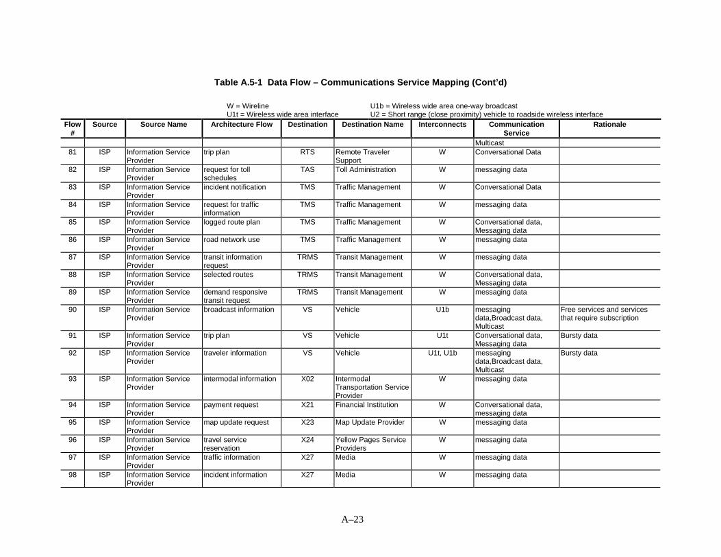
A–23
Table A.5-1 Data Flow – Communications Service Mapping (Cont’d)
W = WirelineU1t = Wireless wide area interface
U1b = Wireless wide area one-way broadcastU2 = Short range (close proximity) vehicle to roadside wireless interface
Flow#
Source Source Name Architecture Flow Destination Destination Name Interconnects CommunicationService
Rationale
Multicast81 ISP Information Service
Providertrip plan RTS Remote Traveler
SupportW Conversational Data
82 ISP Information ServiceProvider
request for tollschedules
TAS Toll Administration W messaging data
83 ISP Information ServiceProvider
incident notification TMS Traffic Management W Conversational Data
84 ISP Information ServiceProvider
request for trafficinformation
TMS Traffic Management W messaging data
85 ISP Information ServiceProvider
logged route plan TMS Traffic Management W Conversational data,Messaging data
86 ISP Information ServiceProvider
road network use TMS Traffic Management W messaging data
87 ISP Information ServiceProvider
transit informationrequest
TRMS Transit Management W messaging data
88 ISP Information ServiceProvider
selected routes TRMS Transit Management W Conversational data,Messaging data
89 ISP Information ServiceProvider
demand responsivetransit request
TRMS Transit Management W messaging data
90 ISP Information ServiceProvider
broadcast information VS Vehicle U1b messagingdata,Broadcast data,Multicast
Free services and servicesthat require subscription
91 ISP Information ServiceProvider
trip plan VS Vehicle U1t Conversational data,Messaging data
Bursty data
92 ISP Information ServiceProvider
traveler information VS Vehicle U1t, U1b messagingdata,Broadcast data,Multicast
Bursty data
93 ISP Information ServiceProvider
intermodal information X02 IntermodalTransportation ServiceProvider
W messaging data
94 ISP Information ServiceProvider
payment request X21 Financial Institution W Conversational data,messaging data
95 ISP Information ServiceProvider
map update request X23 Map Update Provider W messaging data
96 ISP Information ServiceProvider
travel servicereservation
X24 Yellow Pages ServiceProviders
W messaging data
97 ISP Information ServiceProvider
traffic information X27 Media W messaging data
98 ISP Information ServiceProvider
incident information X27 Media W messaging data

A–24
Table A.5-1 Data Flow – Communications Service Mapping (Cont’d)
W = WirelineU1t = Wireless wide area interface
U1b = Wireless wide area one-way broadcastU2 = Short range (close proximity) vehicle to roadside wireless interface
Flow#
Source Source Name Architecture Flow Destination Destination Name Interconnects CommunicationService
Rationale
99 ISP Information ServiceProvider
traffic information X28 Media Operator W messagingdata,Broadcast data,Multicast
100 ISP Information ServiceProvider
incident information X28 Media Operator W messaging data
101 ISP Information ServiceProvider
ISP coord X31 Other ISP W messaging data
102 PIAS Personal InformationAccess
emergency notification EM EmergencyManagement
U1t Conversational data,messaging data, locationdata
Minimum delay in datacommunication for forwardand reverse link mayberequired. Location data foremergency response
103 PIAS Personal InformationAccess
traveler informationrequest
ISP Information ServiceProvider
W,U1t messaging data Bursty messages, Wireless toPDA. Location data for valueadded services.
104 PIAS Personal InformationAccess
trip request ISP Information ServiceProvider
W,U1t Conversational Data,Messaging data
Bursty messages, Wireless toPDA
105 PIAS Personal InformationAccess
trip confirmation ISP Information ServiceProvider
W,U1t Conversational Data,Messaging data
Bursty messages. Wireless toPDA
106 PIAS Personal InformationAccess
yellow pages request ISP Information ServiceProvider
W,U1t Conversational Data,Messaging data
Bursty messages, Wireless toPDA
107 PIAS Personal InformationAccess
demand responsivetransit request
TRMS Transit Management U1t messaging data Bursty messages
108 PIAS Personal InformationAccess
map update request X23 Map Update Provider W,U1t messaging data Service on request or servicesby subscription
109 PMS Parking Management parking lot reservationconfirmation
ISP Information ServiceProvider
W messaging data
110 PMS Parking Management parking availability ISP Information ServiceProvider
W messaging data
111 PMS Parking Management operational data PS Planning Subsystem W messaging data112 PMS Parking Management demand management
price change responseTMS Traffic Management W messaging data
113 PMS Parking Management parking availability TMS Traffic Management W messaging data114 PMS Parking Management transit parking
coordinationTRMS Transit Management W Messaging data
115 PMS Parking Management request tag data VS Vehicle U2 Conversational data Data transfer while in motion,when passing the specificlocations at speeds up to 70mph
116 PMS Parking Management tag update VS Vehicle U2 Conversational data Data transfer while in motion,

A–25
Table A.5-1 Data Flow – Communications Service Mapping (Cont’d)
W = WirelineU1t = Wireless wide area interface
U1b = Wireless wide area one-way broadcastU2 = Short range (close proximity) vehicle to roadside wireless interface
Flow#
Source Source Name Architecture Flow Destination Destination Name Interconnects CommunicationService
Rationale
when passing the specificlocations at speeds up to 70mph
117 PMS Parking Management payment request X21 Financial Institution W Conversational data,messaging data
118 PMS Parking Management parking status X36 Parking Operator W messaging data119 PMS Parking Management parking availability X37 Parking Service
ProviderW messaging data
120 PMS Parking Management violation notification X62 Enforcement Agency W messaging data121 PMS Parking Management license request X64 DMV W Messaging data122 PS Planning Subsystem planning data TMS Traffic Management W messaging data123 PS Planning Subsystem map update request X23 Map Update Provider W Messaging data124 PS Planning Subsystem planning data X25 Transportation
PlannersW messaging data
125 RS Roadway Subsystem pollution data EMMS EmissionsManagement
W messaging data
126 RS Roadway Subsystem fault reports TMS Traffic Management W Conversational data,messaging data
127 RS Roadway Subsystem request for right of way TMS Traffic Management W Conversational Data128 RS Roadway Subsystem vehicle probe data TMS Traffic Management W messaging data129 RS Roadway Subsystem AHS status TMS Traffic Management W messaging data130 RS Roadway Subsystem incident data TMS Traffic Management W messaging data131 RS Roadway Subsystem freeway control status TMS Traffic Management w messaging data132 RS Roadway Subsystem signal control status TMS Traffic Management W messaging data133 RS Roadway Subsystem HOV data TMS Traffic Management W Messaging data134 RS Roadway Subsystem signal priority request TMS Traffic Management W messaging data135 RS Roadway Subsystem local traffic flow TMS Traffic Management W messaging data136 RS Roadway Subsystem AHS control data VS Vehicle U2 messaging data Data transfer while in motion,
when passing the specificlocations at speeds up to 70mph
137 RS Roadway Subsystem vehicle signage data VS Vehicle U2 messaging data Data transfer while in motion,when passing the specificlocations at speeds up to 70mph
138 RS Roadway Subsystem intersection status VS Vehicle U2 messaging data Data transfer while in motion,when passing the specificlocations at speeds up to 70mph
139 RS Roadway Subsystem request tag data VS Vehicle U2 Messaging data

A–26
Table A.5-1 Data Flow – Communications Service Mapping (Cont’d)
W = WirelineU1t = Wireless wide area interface
U1b = Wireless wide area one-way broadcastU2 = Short range (close proximity) vehicle to roadside wireless interface
Flow#
Source Source Name Architecture Flow Destination Destination Name Interconnects CommunicationService
Rationale
140 RS Roadway Subsystem grant right of wayand/or stop traffic
X29 Multimodal Crossings W Conversational data,messaging data
141 RTS Remote TravelerSupport
emergency notification EM EmergencyManagement
W,U1t Conversational speech,messaging data, locationdata
RTS can be a transportableunit. Location data emergencyresponse.
142 RTS Remote TravelerSupport
yellow pages request ISP Information ServiceProvider
W Conversational data,Messaging Data
143 RTS Remote TravelerSupport
trip request ISP Information ServiceProvider
W Conversational Data
144 RTS Remote TravelerSupport
traveler informationrequest
ISP Information ServiceProvider
W messaging data
145 RTS Remote TravelerSupport
demand responsivetransit request
ISP Information ServiceProvider
W messaging data
146 RTS Remote TravelerSupport
emergency notification TRMS Transit Management W Conversational data,Messaging Data
147 RTS Remote TravelerSupport
transit request TRMS Transit Management W messaging data
148 RTS Remote TravelerSupport
traveler informationrequest
TRMS Transit Management W messaging data
149 RTS Remote TravelerSupport
map update request X23 Map Update Provider W messaging data
150 TAS Toll Administration toll schedules ISP Information ServiceProvider
W messaging data
151 TAS Toll Administration operational data PS Planning Subsystem W messaging data152 TAS Toll Administration toll instructions TCS Toll Collection W messaging data153 TAS Toll Administration demand management
price change responseTMS Traffic Management W messaging data
154 TAS Toll Administration probe data TMS Traffic Management W messaging data156 TAS Toll Administration payment request X21 Financial Institution W messaging data157 TAS Toll Administration toll revenues and
summary reportsX44 Toll Service Provider W messaging data
158 TAS Toll Administration violation notification X62 Enforcement Agency W messaging data159 TAS Toll Administration license request X64 DMV W messaging data160 TCS Toll Collection toll transactions TAS Toll Administration W messaging data161 TCS Toll Collection tag update VS Vehicle U2 Conversational Data Data communication while
passing by specific locationsat speeds up to 70 mph
162 TCS Toll Collection request tag data VS Vehicle U2 Conversational data Data communication whilepassing by specific locationsat speeds up to 70 mph

A–27
Table A.5-1 Data Flow – Communications Service Mapping (Cont’d)
W = WirelineU1t = Wireless wide area interface
U1b = Wireless wide area one-way broadcastU2 = Short range (close proximity) vehicle to roadside wireless interface
Flow#
Source Source Name Architecture Flow Destination Destination Name Interconnects CommunicationService
Rationale
163 TMS Traffic Management incident informationrequest
EM EmergencyManagement
W Messaging data
164 TMS Traffic Management incident notification EM EmergencyManagement
W Messaging data
165 TMS Traffic Management pollution state datarequest
EMMS EmissionsManagement
W messaging data
166 TMS Traffic Management traffic information ISP Information ServiceProvider
W messaging data
167 TMS Traffic Management parking instructions PMS Parking Management W messaging data168 TMS Traffic Management demand management
price change requestPMS Parking Management W messaging data
169 TMS Traffic Management operational data PS Planning Subsystem W messaging data170 TMS Traffic Management freeway control data RS Roadway Subsystem W messaging data171 TMS Traffic Management signal control data RS Roadway Subsystem W messaging data172 TMS Traffic Management AHS control
informationRS Roadway Subsystem W messaging data
173 TMS Traffic Management signage data RS Roadway Subsystem W messaging data174 TMS Traffic Management demand management
price change requestTAS Toll Administration W messaging data
175 TMS Traffic Management traffic information TRMS Transit Management W messaging data176 TMS Traffic Management demand management
price change requestTRMS Transit Management W messaging data
177 TMS Traffic Management signal priority status TRMS Transit Management W Conversational data,messaging data
178 TMS Traffic Management event confirmation X19 Event Promoters W messaging data179 TMS Traffic Management map update request X23 Map Update Provider W messaging data180 TMS Traffic Management TMC coord. X35 Other TM W messaging data181 TMS Traffic Management violation notification X62 Enforcement Agency W messaging data182 TMS Traffic Management license request X64 DMV W messaging data183 TRMS Transit Management security alarms EM Emergency
ManagementW Conversational data,
messaging data, locationdata
Location data for emergencyresponse
184 TRMS Transit Management demand responsivetransit plan
ISP Information ServiceProvider
W Conversational data,messaging data
185 TRMS Transit Management transit and fareschedules
ISP Information ServiceProvider
W messaging data
186 TRMS Transit Management transit requestconfirmation
ISP Information ServiceProvider
W messaging data
187 TRMS Transit Management demand responsivetransit route
PIAS Personal InformationAccess
W,U1t messaging data Bursty data

A–28
Table A.5-1 Data Flow – Communications Service Mapping (Cont’d)
W = WirelineU1t = Wireless wide area interface
U1b = Wireless wide area one-way broadcastU2 = Short range (close proximity) vehicle to roadside wireless interface
Flow#
Source Source Name Architecture Flow Destination Destination Name Interconnects CommunicationService
Rationale
188 TRMS Transit Management parking lot transitresponse
PMS Parking Management W messagingdata,Broadcast data,Multicast
189 TRMS Transit Management operational data PS Planning Subsystem W messaging data190 TRMS Transit Management traveler information RTS Remote Traveler
SupportW messaging data,
Multicast data191 TRMS Transit Management transit and fare
schedulesRTS Remote Traveler
SupportW messaging data,
Multicast data192 TRMS Transit Management emergency
acknowledgeRTS Remote Traveler
SupportW Conversational data,
messaging data193 TRMS Transit Management request for transit
signal priorityTMS Traffic Management W messaging data
194 TRMS Transit Management demand managementprice change response
TMS Traffic Management W messaging data
195 TRMS Transit Management emergencyacknowledge
TRVS Transit VehicleSubsystem
U1t Conversational data,messaging data
Minimum delay may berequired
196 TRMS Transit Management driver instructions TRVS Transit VehicleSubsystem
U1t messaging data
197 TRMS Transit Management bad tag list TRVS Transit VehicleSubsystem
U1t messaging data Bursty data
198 TRMS Transit Management request for vehiclemeasures
TRVS Transit VehicleSubsystem
U1t,U2 Conversational data,messaging data
Bursty data using wideareawireless or short rang whilepassing by specific locationsat speeds up to 70 mph
199 TRMS Transit Management schedules, fare inforequest
TRVS Transit VehicleSubsystem
U1t messaging data Bursty data
200 TRMS Transit Management traveler information TRVS Transit VehicleSubsystem
U1t messaging data Bursty data
201 TRMS Transit Management route assignment TRVS Transit VehicleSubsystem
U1t,U2 messaging data Bursty data using wideareawireless or short rang whilepassing by specific locationsat speeds up to 70 mph
202 TRMS Transit Management intermodal information X02 IntermodalTransportation ServiceProvider
W messaging data
203 TRMS Transit Management payment request X21 Financial Institution W Conversational data,messaging data
204 TRMS Transit Management map update request X23 Map Update Provider W messaging data205 TRMS Transit Management TRMS coord X33 Other TRM W messaging data206 TRMS Transit Management camera control X42 Secure Area W Conversational data,
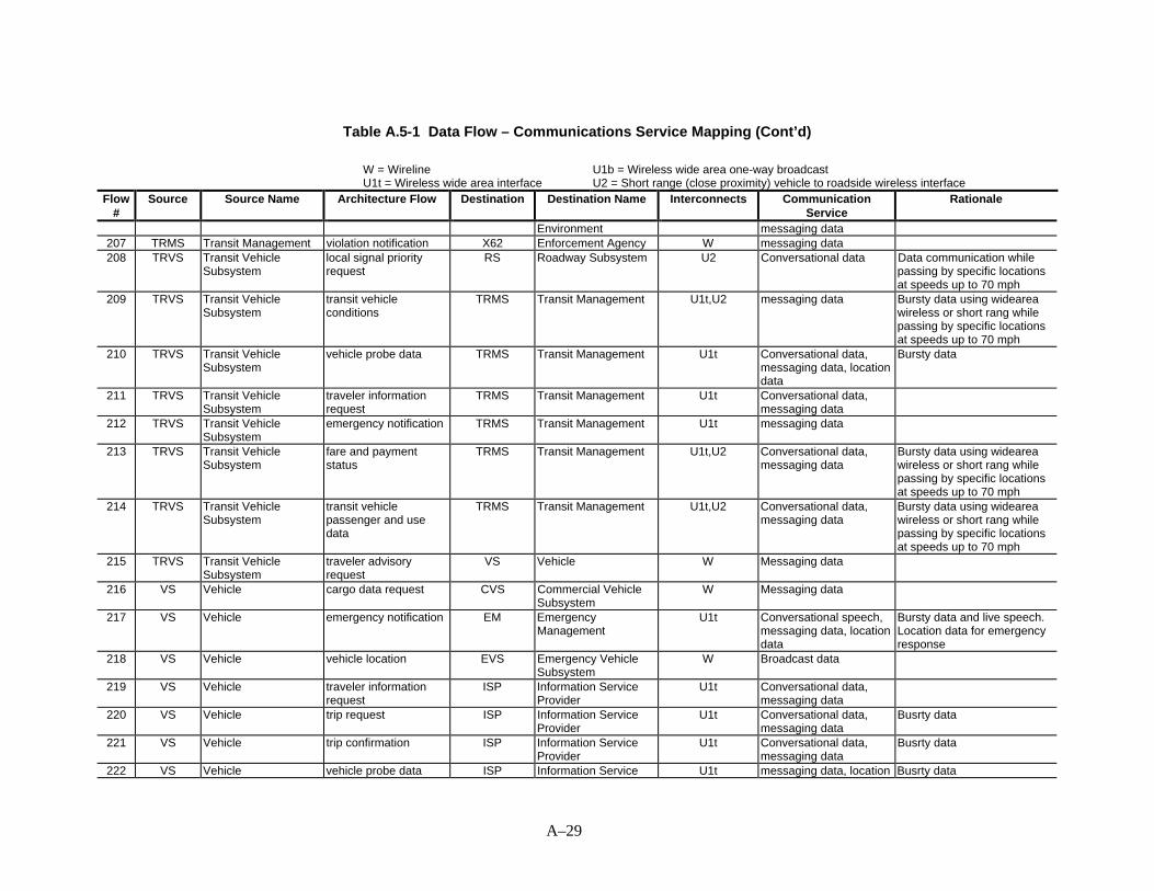
A–29
Table A.5-1 Data Flow – Communications Service Mapping (Cont’d)
W = WirelineU1t = Wireless wide area interface
U1b = Wireless wide area one-way broadcastU2 = Short range (close proximity) vehicle to roadside wireless interface
Flow#
Source Source Name Architecture Flow Destination Destination Name Interconnects CommunicationService
Rationale
Environment messaging data207 TRMS Transit Management violation notification X62 Enforcement Agency W messaging data208 TRVS Transit Vehicle
Subsystemlocal signal priorityrequest
RS Roadway Subsystem U2 Conversational data Data communication whilepassing by specific locationsat speeds up to 70 mph
209 TRVS Transit VehicleSubsystem
transit vehicleconditions
TRMS Transit Management U1t,U2 messaging data Bursty data using wideareawireless or short rang whilepassing by specific locationsat speeds up to 70 mph
210 TRVS Transit VehicleSubsystem
vehicle probe data TRMS Transit Management U1t Conversational data,messaging data, locationdata
Bursty data
211 TRVS Transit VehicleSubsystem
traveler informationrequest
TRMS Transit Management U1t Conversational data,messaging data
212 TRVS Transit VehicleSubsystem
emergency notification TRMS Transit Management U1t messaging data
213 TRVS Transit VehicleSubsystem
fare and paymentstatus
TRMS Transit Management U1t,U2 Conversational data,messaging data
Bursty data using wideareawireless or short rang whilepassing by specific locationsat speeds up to 70 mph
214 TRVS Transit VehicleSubsystem
transit vehiclepassenger and usedata
TRMS Transit Management U1t,U2 Conversational data,messaging data
Bursty data using wideareawireless or short rang whilepassing by specific locationsat speeds up to 70 mph
215 TRVS Transit VehicleSubsystem
traveler advisoryrequest
VS Vehicle W Messaging data
216 VS Vehicle cargo data request CVS Commercial VehicleSubsystem
W Messaging data
217 VS Vehicle emergency notification EM EmergencyManagement
U1t Conversational speech,messaging data, locationdata
Bursty data and live speech.Location data for emergencyresponse
218 VS Vehicle vehicle location EVS Emergency VehicleSubsystem
W Broadcast data
219 VS Vehicle traveler informationrequest
ISP Information ServiceProvider
U1t Conversational data,messaging data
220 VS Vehicle trip request ISP Information ServiceProvider
U1t Conversational data,messaging data
Busrty data
221 VS Vehicle trip confirmation ISP Information ServiceProvider
U1t Conversational data,messaging data
Busrty data
222 VS Vehicle vehicle probe data ISP Information Service U1t messaging data, location Busrty data

A–30
Table A.5-1 Data Flow – Communications Service Mapping (Cont’d)
W = WirelineU1t = Wireless wide area interface
U1b = Wireless wide area one-way broadcastU2 = Short range (close proximity) vehicle to roadside wireless interface
Flow#
Source Source Name Architecture Flow Destination Destination Name Interconnects CommunicationService
Rationale
Provider data223 VS Vehicle yellow pages request ISP Information Service
ProviderU1t Conversational data,
messaging data224 VS Vehicle tag data PMS Parking Management U2 Conversational data Data communication while
passing by specific locationsat speeds up to 70 mph
225 VS Vehicle AHS vehicle data RS Roadway Subsystem U2 Conversational data Data communication whilepassing by specific locationsat speeds up to 70 mph
226 VS Vehicle vehicle probe data RS Roadway Subsystem U2 Messaging Data Data communication whilepassing by specific locationsat speeds up to 70 mph
227 VS Vehicle tag data TCS Toll Collection U2 Conversational data Data communication whilepassing by specific locationsat speeds up to 70 mph
228 VS Vehicle vehicle location TRVS Transit VehicleSubsystem
W Broadcast data
229 VS Vehicle vehicle control X03 Basic Vehicle W Conversational Data230 VS Vehicle map update request X23 Map Update Provider U1t messaging data Busrty data231 X01 Intermodal Freight
Shipperintermod CVO coord FMS Fleet and Freight
ManagementW messaging data
232 X02 IntermodalTransportation ServiceProvider
intermodal information ISP Information ServiceProvider
W messaging data
233 X02 IntermodalTransportation ServiceProvider
intermodal information TRMS Transit Management W messaging data
234 X03 Basic Vehicle vehicle measures VS Vehicle W Broadcast data235 X08 Commercial Vehicle vehicle measures CVS Commercial Vehicle
SubsystemW Broadcast data
236 X10 CVO Inspector CVC override mode CVCS Commercial VehicleCheck
U2 Conversational data,messaging data
237 X13 E911 or ETS incident information EM EmergencyManagement
W Conversational dataconversational speec,location data
Location data for emergencyresponse
238 X19 Event Promoters event plans TMS Traffic Management W messaging data,Multicast data
239 X21 Financial Institution transaction status CVAS Commercial VehicleAdministration
W Conversational data,messaging data
240 X21 Financial Institution transaction status ISP Information Service W Conversational data,
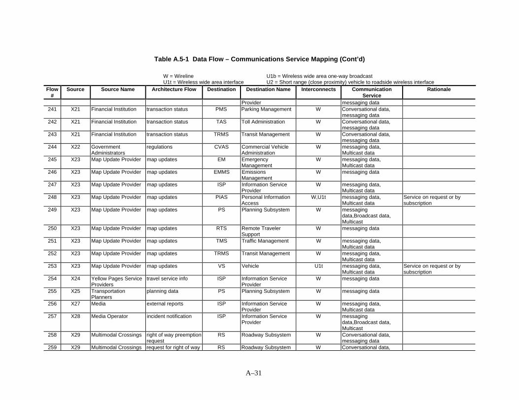
A–31
Table A.5-1 Data Flow – Communications Service Mapping (Cont’d)
W = WirelineU1t = Wireless wide area interface
U1b = Wireless wide area one-way broadcastU2 = Short range (close proximity) vehicle to roadside wireless interface
Flow#
Source Source Name Architecture Flow Destination Destination Name Interconnects CommunicationService
Rationale
Provider messaging data241 X21 Financial Institution transaction status PMS Parking Management W Conversational data,
messaging data242 X21 Financial Institution transaction status TAS Toll Administration W Conversational data,
messaging data243 X21 Financial Institution transaction status TRMS Transit Management W Conversational data,
messaging data244 X22 Government
Administratorsregulations CVAS Commercial Vehicle
AdministrationW messaging data,
Multicast data245 X23 Map Update Provider map updates EM Emergency
ManagementW messaging data,
Multicast data246 X23 Map Update Provider map updates EMMS Emissions
ManagementW messaging data
247 X23 Map Update Provider map updates ISP Information ServiceProvider
W messaging data,Multicast data
248 X23 Map Update Provider map updates PIAS Personal InformationAccess
W,U1t messaging data,Multicast data
Service on request or bysubscription
249 X23 Map Update Provider map updates PS Planning Subsystem W messagingdata,Broadcast data,Multicast
250 X23 Map Update Provider map updates RTS Remote TravelerSupport
W messaging data
251 X23 Map Update Provider map updates TMS Traffic Management W messaging data,Multicast data
252 X23 Map Update Provider map updates TRMS Transit Management W messaging data,Multicast data
253 X23 Map Update Provider map updates VS Vehicle U1t messaging data,Multicast data
Service on request or bysubscription
254 X24 Yellow Pages ServiceProviders
travel service info ISP Information ServiceProvider
W messaging data
255 X25 TransportationPlanners
planning data PS Planning Subsystem W messaging data
256 X27 Media external reports ISP Information ServiceProvider
W messaging data,Multicast data
257 X28 Media Operator incident notification ISP Information ServiceProvider
W messagingdata,Broadcast data,Multicast
258 X29 Multimodal Crossings right of way preemptionrequest
RS Roadway Subsystem W Conversational data,messaging data
259 X29 Multimodal Crossings request for right of way RS Roadway Subsystem W Conversational data,

A–32
Table A.5-1 Data Flow – Communications Service Mapping (Cont’d)
W = WirelineU1t = Wireless wide area interface
U1b = Wireless wide area one-way broadcastU2 = Short range (close proximity) vehicle to roadside wireless interface
Flow#
Source Source Name Architecture Flow Destination Destination Name Interconnects CommunicationService
Rationale
messaging data260 X30 Other EM emergency
coordinationEM Emergency
ManagementW Conversational data,
messaging data261 X31 Other ISP ISP coord ISP Information Service
ProviderW messaging data
262 X33 Other TRM TRMS coord TRMS Transit Management W messaging data263 X35 Other TM TMC coord. TMS Traffic Management W messaging data264 X37 Parking Service
Providerrequest forperformance data
PMS Parking Management W messaging data
265 X51 Transit Vehicle vehicle measures TRVS Transit VehicleSubsystem
W Broadcast data
266 X58 Weather Service weather information ISP Information ServiceProvider
W messagingdata,Broadcast data,Multicast
267 X58 Weather Service weather information TMS Traffic Management W messagingdata,Broadcast data,Multicast
268 X59 Other CVAS CVAS informationexchange
CVAS Commercial VehicleAdministration
W messaging data
269 X59 Other CVAS credentials and safetyinformation response
CVAS Commercial VehicleAdministration
W messaging data
270 X60 Intermodal FreightDepot
intermod CVO coord FMS Fleet and FreightManagement
W messaging data
271 X64 DMV registration CVAS Commercial VehicleAdministration
W messaging data
272 X64 DMV vehicle characteristics PMS Parking Management W Messaging data273 X64 DMV registration TAS Toll Administration W messaging data274 X64 DMV registration TMS Traffic Management W messaging data275 X65 CVO Information
Requestorcredentials and safetyinformation request
CVAS Commercial VehicleAdministration
W messaging data

B–1
APPENDIX B ARCHITECTURE INTERCONNECT DIAGRAMS
LEVEL 1
Using the AID template and the Data Flow - Communication Services Mapping table presentedin Appendix A, a sample set of the data flows are represented in an Architecture InterconnectDiagram (AID) format. Each AID may represent more than one data flow. Whereas many of theAIDs support messaging and conversational data, in many cases they can also be supported byconversational speech. In fact, near-term deployments of applications like pre-trip planning oren-route driver advisories will probably disseminate information verbally rather than via bitstreams. Thus providing for this in the analysis supports both rural deployments, and earlydeployment in any location. In rural areas providing new infrastructure will most likely beexpensive until enough other demand is reached or older existing equipment must be replaced.
The substantiation for the operation mode is based on the nature of the data flow (e.g.,anticipated frequency of use, message length, qualitative rationale). The operation mode wasrefined and calibrated with information from Section 6, Data Loading Analysis.
Figures B-1 through B-17 are a sample set of the AIDs for the inter-entity links, indicating thephysical medium, wireline (w) or wireless (u1, u2, u3) and the mode of operation (e.g., circuit,packet) and carrying forward the service types (conversational speech, conversational data,messaging data, broadcast data and/or multicast data) from the Data Flow - CommunicationServices Mapping Table. The figures show the flow from the left entity to the right entity, unlessspecifically indicated for that flow (which occurs when there are flows in both directions).

B–2
EmergencyManagementSubsystem(EM)
Wireless wide area interface (U1t)EmergencyVehicleSubsystem(EVS)
Bursty data or live speech. Low delay in data comm.may be required∧Data Flow: Emergency dispatch requests
Assigned route,Hazmat information &Emergency vehicle driver status updateEmergency vehicle driver inputsemergency vehicle dispatch ack.
---->---->----><----<----<----
Service Conversational speech, Messaging dataOperational Mode
Circuit, Packet
Figure B-1 First Level EM - EVS AID
PersonalInformationAccessSubsystem(PIAS)
Wireless wide area interface (U1t)Wireline (W)
EmergencyManagementSubsystem (EM)
Low delay in data communication may be required∧Data Flow: Emergency notification &
Emergency status-----><-----
Service Conversational data,Messaging data
Operational Mode Circuit, Packet
Figure B-2 First Level PIAS-EM AID

B–3
PersonalInformationAccessSubsystem(PIAS)
Wireless wide area interface (U1t)Wireline (W)
TransitManagementSubsystem (TRMS)
∧Data Flow: demand responsive transit
requestDemand responsive transitroute
------->
<------
Service Messaging dataOperational Mode Circuit, Packet
Figure B-3 First Level PIAS-TRMS AID
RemoteTravelerSupportSubsystem(RTS)
Wireless wide area interface (U1t)Wireline (W)
EmergencyManagementSubsystem (EM)
Wide area wireless communication totransportable units∧
Data Flow: Emergency notification &Emergency ack.
------><------
Service Conversational speech,Messaging data
Operational Mode Circuit, Packet
Figure B-4 First Level RTS-EM AID

B–4
ParkingmanagementSubsystem(PMS)
Wireline (W)Information ServiceProvider (ISP)
∧Data Flow: Parking availability &
parking reservationParking lot data requestParking reservationrequest
----->-----><-----<-----
Service Messaging dataOperational Mode Circuit, Packet
Figure B-5 First Level PMS-ISP AID
ParkingmanagementSubsystem(PMS)
Wireline (W)TrafficManagementSubsystem (TMS)
∧Data Flow: Parking availability &
Parking instructionsprice change req. /demandmang.
-----><-----<-----
Service Messaging dataOperational Mode Circuit, Packet
Figure B-6 First Level PMS-TMS AID

B–5
ParkingmanagementSubsystem(PMS)
Vehicle to road side interface (U2)VehicleSubsystem (VS)
Data transfer while in motion, when passing thespecific locations at speeds up to 70 mph∧
Data Flow: Request tag datatag updatetag data
----->-----><----
Service Conversational dataOperational Mode Packet
Figure B-7 First Level PMS-VS AID
InformationServiceProvider(ISP)
Wireline (W)EmergencyManagementSubsystem (EM)
Minimum delay in data communication may berequired∧
Data Flow: Emerg. vehicle routeIncident inf. req.Request for emergency routeIncident inf.
----->-----><----<----
Service Conversational data, &Messaging data
Operational Mode Circuit, Packet
Figure B-8 First Level ISP-EM AID

B–6
InformationServiceProvider(ISP)
Wireline (W)TransitManagementSubsystem(TRMS)
Information on request, free and services that requiresubscription.∧
Data Flow: selected routedemand responsive transit plan
-----><----
Service Messaging data, conversationaldata
Operational Mode Circuit, Packet
Data Flow: demand responsive transit req.transit information requesttransit req. confirmationtransit and fare schedule
----->-----><----<----
Service Messaging data
Operational Mode Circuit, Packet
Figure B-9 First Level ISP-TRMS AID
InformationServiceProvider(ISP)
Wireline (W)Traffic ManagementSubsystem (TMS)
∧Data Flow: incident notification
Request for traffic inf.road network useLogged route planTraffic information
----->----->----->-----><-----
Service Messaging data,conversational data
Operational Mode Circuit, Packet
Figure B-10 First Level ISP-TMS AID

B–7
InformationServiceProvider(ISP)
Wireline (W)Fleet ManagementSubsystem (FMS)
∧Data Flow: Route plan &
Route request------><-----
Service Messaging dataOperational Mode Circuit, Packet
Figure B-11 First Level ISP-FMS AID
InformationServiceProvider(ISP)
Wireless Wide area interface (U1t)VehicleSubsystem (VS)
Bursty data, free services & services that requiresubscription∧
Data Flow: Traveler informationBroadcast informationtrip plan
----->----->----->
Service Messaging data, broadcast &multicast
Operational Mode Circuit, Packet
Data Flow: Vehicle probe dataTraveler inf. requesttrip requesttrip confirmationYellow page request
<------<------<------<------<------
Service Messaging data,conversational data & location
Operational Mode Circuit, Packet
Figure B-12 First Level ISP-VS AID

B–8
TrafficManagementSubsystem(TMS)
Wireline (W)Transit ManagementSubsystem (TRMS)
∧Data Flow: signal priority status
Traffic informationdemand mang. pricechange req.Req. for transit signalpriority.demand mang. pricechange
------>------>------>
<----
<----
Service Messaging data,conversational data
Operational Mode Circuit, Packet
Figure B-13 First Level TMS-TRMS AID
TrafficManagementSubsystem(TMS)
Wireline (W)EmergencyManagementSubsystem (EM)
Minimum delay in data communication may berequired∧
Data Flow: incident inf. requestincident notificationincident informationEmergency veh. greenwave req.Incident notification
----->-----><-----<-----<-----
Service Conversational data, Messagingdata
Operational Mode Circuit, Packet
Figure B-14 First Level TMS-EM AID
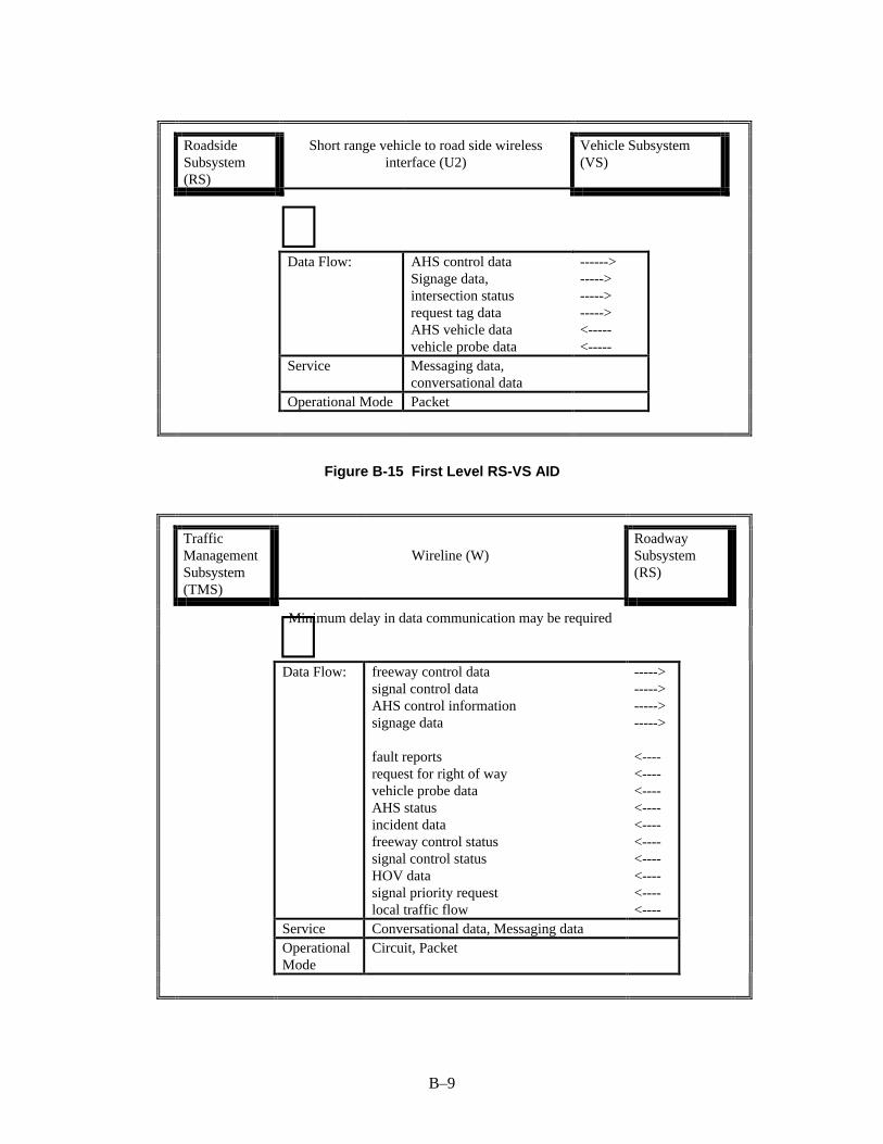
B–9
RoadsideSubsystem(RS)
Short range vehicle to road side wirelessinterface (U2)
Vehicle Subsystem(VS)
∧Data Flow: AHS control data
Signage data,intersection statusrequest tag dataAHS vehicle datavehicle probe data
------>----->----->-----><-----<-----
Service Messaging data,conversational data
Operational Mode Packet
Figure B-15 First Level RS-VS AID
TrafficManagementSubsystem(TMS)
Wireline (W)RoadwaySubsystem(RS)
Minimum delay in data communication may be required∧Data Flow: freeway control data
signal control dataAHS control informationsignage data
fault reportsrequest for right of wayvehicle probe dataAHS statusincident datafreeway control statussignal control statusHOV datasignal priority requestlocal traffic flow
----->----->----->----->
<----<----<----<----<----<----<----<----<----<----
Service Conversational data, Messaging dataOperationalMode
Circuit, Packet

B–10
Figure B-16 First Level TMS-RS AID
TrafficManagementSubsystem(TMS)
Wireline (W)EmissionManagementSubsystem (EMMS)
∧Data Flow: pollution state data request &
widearea statistical pollutioninformation
------><-------
Service Conversational speech,Messaging data
Operational Mode Circuit, Packet
Figure B-17 First Level TMS-EMMS AID

C–1
APPENDIX C COMMUNICATION ARCHITECTURE RENDITIONS
AND APPLICABLE TECHNOLOGIES
Section C.1 of this appendix provides information that represents the next step in thecommunications architecture design process – the development of the CommunicationArchitecture Renditions. This activity is denoted as the highlighted block in Figure C.0-1. Thearchitecture renditions are essentially examples of how to provide connections between usersbased on the communications network reference model and the evaluations of feasibleimplementations. In addition, to save the re-listing of the renditions, each rendition is combinedwith the listing of the data flows supported by that rendition. This effectively provides a mapbetween the renditions and the Architecture Interconnect Diagrams (AIDs). Section C.2 providesan example of mapping applicable communication technologies to the renditions.

C–2
Map DataFlows-CommunicationServices
DevelopArchitectureInterconnectDiagrams (AID)
DevelopNetworkReferenceModel
DevelopArchitectureRenditions(AR)
MapAID -AR
RecommendTechnologyCandidates
LogicalCommunicationFunctions
PhysicalCommunicationEntities
Feasibility &CostConstraints
ArchitectureInterconnectSpecifications
TechnologyAssessment
Figure C.0-1 Communications Architecture Development Process – DevelopArchitecture Renditions
C.1 Format/Purpose
The previous sections have identified the physical entities and the communication servicesrequired between them. The task now is to show how user-to-user communication paths are builtup from combinations of the identified wireline and wireless links, and to show that the user'sneeds are met by the identified communication services. This is accomplished by establishing aset of renditions which illustrate the connectivities provided by w and u links. A Level 1rendition is generated for each of the possible interconnections between these services, exceptthree which do not meet the needs of the architecture. Again the Level 0 Rendition, which showsthe full connectivity between users over multiple links, appears before the Level 1 renditionsfrom which it was developed.
C.1.1 Level 0 Rendition
The Level 0 rendition (Figure C.1-1) represents a composition of all the renditions to reflect thecombined needs of the architecture. The left side shows a general user with any one or all fourpossible communication links and how those links connect the user to other users.
The Level 0 Rendition shows a generic user communicating to another user over one of the fourcommunication types (w, u1, u2, u3), where the medium/long and short distance radio basedcommunication (u1 and u2, respectively) travels through a base station (the wireline almostwithout exception will pass through a central office or at least a user concentrator/switch) and thevehicle-to-vehicle radio (u3) uses no intermediary.

C–3
User
Central Office
Base Station
Base Station
Rendition 1
u1
w, u1
Rendition 2
u2
w
Rendition 4
w
Rendition 3
u3
Candidate Technologiesfor u1 interface
(Example)Terrestrial systems•FM subcarrierCellular based systems•CDPD•ESMR, RAM, ARDIS•Two-way paging
Candidate Technologiesfor w interface
(Example)Public Networks•PSTN, ISDNPrivate networks•SONET, ATM
Candidate Technologiesfor u2 interface
(Example)•Active RF•Passive RF•Infrared
User
User
Figure C.1-1 Level 0 Rendition
C.1.2 Level 1 Rendition
Figure C.1-2 illustrates the interaction between the users and the underlying communicationarchitecture. Given the choice of communication services and operation modes (i.e., circuitversus packet versus non-switched), several renditions of this general model are possible (thesemay be supported by a single communication infrastructure).

C–4
IVHS USER
IVHS USER
LOGICAL INFORMATION TRANSFER
(DATA FLOW)
TRANSPORTATION
UP
PSTN
ISDN UD
COMMUNICATION
WBS Switch
Internet
Control Flow Control Flow
Terminal &Transceiver
User Device
WC
PDN
Dedicated connection
IWF
Figure C.1-2 Communication Architecture – Transportation Layer Interaction
The communication architecture in Figure C.1-2 shows multiple functions necessary to deliverdata from or to a mobile ITS user to or from a stationary user, respectively. Because the pathfrom stationary user to stationary user makes use of the wireline component in all but a few dataflows, the best path makes use of the existing infrastructure provided by public communicationsservice providers such as the local Telco in all but a few exceptional locations. In those locationsITS users may deploy their own dedicated system; even then that connection will beinterconnected to, and therefore appear as an extension of, the existing public system.
To simplify the presentation, the end-to-end model represented by Figure C.1-2 is broken intothose types which are of direct interest to the ITS architecture: the u1, u2, u3, and w, those at eachend of the link for which the interface to the communications service provider is not transparentto the system. Thus four renditions are given, one for each of the u and w types of link. Thegathering deployment of digital cellular and other digital radio technologies bolsters theassumption that the tetherless (mobile) user will have a digital connection to other usersconnected to the group of base stations and, in most locations, to the local communicationsservice provider.
Rendition 1: (u1)The u1 link is required to provide (part way) service between tetherless and both other tetherlessusers and stationary users. The u1 link includes the two-way wireless link u1t and the broadcastlink u1b. As shown in Figure C.1-3a, the u1t link end-to-end service for tetherless users connectedto the same base station or base stations with dedicated connections. In the near term this ismostly an analog service but evolving to digital over the next few years. The service may useone or more of the technologies listed in Appendix D, Technology Survey and Assessment.When users have different technologies not supported by the same base station, the publicswitched network (PSTN) typically provides the connection between the different base stations.For communication between tetherless and stationary users, the u1t link connects the tetherlessuser to the base station and the public telco. The wireline portion of the connection is consideredsecondary to the wireless link in its criticality.

C–5
u1t interconnection between tetherless users and stationary users would be digital except in someinstances (including rural where the local telco service has not yet been digitized). In that case,while the fixed portion of the network supports circuit-mode operation, it cannot exchange digitalsignals. A modem bank interconnected to the Mobile Switching Center (MSC) initiates a callsetup to the target application. A modem at the target user converts the signal to digital data. Acall from a stationary user is routed through the telco or one of the Internet-like networks to thebase station in the reverse process and then a channel, either circuit-switched (primarily for voiceor large messages) or packet-switched (primarily for data but also voice) to the tetherless user isidentified. Thus, the logical connection between the two users in the transportation plane issatisfied. Because of the short nature of all currently identified messages, most will use packetswitching whenever that option is available. This rendition supports the data flows, listed inTable C.1-1a.
Figure C.1-3b depicts the rendition for u1b . This link can support low rate one-way wireless dataservices. It uses broadcast services which include paging and FM subcarrier technology fortransmitting data to subscribers over the paging and FM frequency channels. From Figure C.1-3b, the broadcast data is processed (in the message processor) and distributed to the selectedpaging or FM broadcast stations. Broadcast stations encode and modulate the data using pagingor FM subcarrier modulation format, as described in Section 7.
WIRELESS CONTROLLER
BASE STATIONs• • •
FIXED NETWORK
OAM&P
1t
USER TERMINAL • • •
OTHER PACKET SWITCH
MODEM BANK
PACKET SWITCH
CIRCUIT SWITCH
OTHER CIRCUIT SWITCH
USER TERMINAL
USER TERMINAL
T1
Packet mode Rendition for U1t supports: - messaging data, - multicast data,
Circuit mode Rendition for U1t supports: - conversational speech, - conversational data
u
Figure C.1-3a Rendition 1 — u1t, Two-Way Wide-Area Wireless Link

C–6
Broadcast Message Processor
FM Broadcast StationsData Encoder &
Subcarrier Generator
Data Distribution Network
Message EntrySystem
UserTerminal
UserTerminal
UserTerminal
U1b
Broadcast Mode Renditionfor U1b support: - Broadcast Data
Paging Broadcast StationsData Encoder & Modulator
Figure C.1-3b Rendition 1 — u1b, One-way Wide-Area Wireless Link

C–7
Table C.1-1a Wireless Wide Area Data Flows (u 1t)
Flow # Source Source Name Architecture Flow Destination Destination Name Interconnects CommunicationService
Rationale
33 CVS Commercial VehicleSubsystem
driver and vehicleinformation
FMS Fleet and FreightManagement
U1t messaging data,location data
bursty transactions
37 EM EmergencyManagement
emergency dispatchrequests
EVS Emergency VehicleSubsystem
U1t Conversational speech,messaging data
Low delay bursty data orconversational speech
38 EM EmergencyManagement
assigned route EVS Emergency VehicleSubsystem
U1t Conversational speech,messaging data
Low delay bursty data orconversational speech
39 EM EmergencyManagement
Hazmat information EVS Emergency VehicleSubsystem
U1t Conversational speech,messaging data
Low delay bursty data orconversational speech
50 EM EmergencyManagement
emergencyacknowledge
VS Vehicle U1t Conversational dataconversational speec
Low delay bursty data
58 EVS Emergency VehicleSubsystem
emergency vehicledriver status update
EM EmergencyManagement
U1t messaging data Low delay bursty data orlive voice.
59 EVS Emergency VehicleSubsystem
emergency vehicledriver inputs
EM EmergencyManagement
U1t Conversational speech,messaging data
Bursty data or live voice.Minimum delay in datacommunication forforward and reverse linkmay be required
60 EVS Emergency VehicleSubsystem
emergency vehicledispatch acknowledge
EM EmergencyManagement
U1t Conversational speech,messaging data
Bursty data or live voice.Minimum delay in datacommunication forforward and reverse linkmay be required
65 FMS Fleet and FreightManagement
fleet to driver update CVS Commercial VehicleSubsystem
U1t messaging data Bursty data
91 ISP Information ServiceProvider
trip plan VS Vehicle U1t Conversational data,Messaging data
Bursty data
92 ISP Information ServiceProvider
traveler information VS Vehicle U1t messagingdata,Broadcast data,Multicast
Bursty data
102 PIAS Personal InformationAccess
emergencynotification
EM EmergencyManagement
U1t Conversational data,messaging data,location data
Minimum delay in datacommunication forforward and reverse linkmaybe required.Location data foremergency response
107 PIAS Personal InformationAccess
demand responsivetransit request
TRMS Transit Management U1t messaging data Bursty messages
195 TRMS Transit Management emergencyacknowledge
TRVS Transit VehicleSubsystem
U1t Conversational data,messaging data
Minimum delay may berequired
196 TRMS Transit Management driver instructions TRVS Transit VehicleSubsystem
U1t messaging data
197 TRMS Transit Management bad tag list TRVS Transit VehicleSubsystem
U1t messaging data Bursty data
199 TRMS Transit Management schedules, fare inforequest
TRVS Transit VehicleSubsystem
U1t messaging data Bursty data
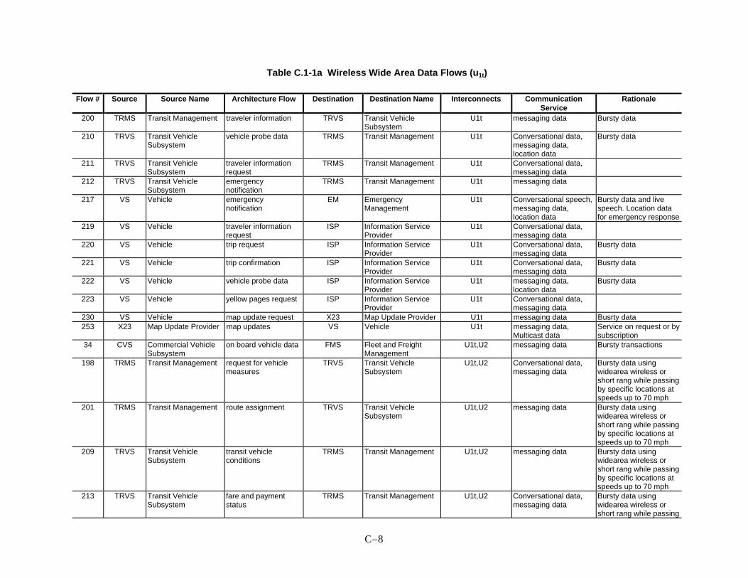
C–8
Table C.1-1a Wireless Wide Area Data Flows (u 1t)
Flow # Source Source Name Architecture Flow Destination Destination Name Interconnects CommunicationService
Rationale
200 TRMS Transit Management traveler information TRVS Transit VehicleSubsystem
U1t messaging data Bursty data
210 TRVS Transit VehicleSubsystem
vehicle probe data TRMS Transit Management U1t Conversational data,messaging data,location data
Bursty data
211 TRVS Transit VehicleSubsystem
traveler informationrequest
TRMS Transit Management U1t Conversational data,messaging data
212 TRVS Transit VehicleSubsystem
emergencynotification
TRMS Transit Management U1t messaging data
217 VS Vehicle emergencynotification
EM EmergencyManagement
U1t Conversational speech,messaging data,location data
Bursty data and livespeech. Location datafor emergency response
219 VS Vehicle traveler informationrequest
ISP Information ServiceProvider
U1t Conversational data,messaging data
220 VS Vehicle trip request ISP Information ServiceProvider
U1t Conversational data,messaging data
Busrty data
221 VS Vehicle trip confirmation ISP Information ServiceProvider
U1t Conversational data,messaging data
Busrty data
222 VS Vehicle vehicle probe data ISP Information ServiceProvider
U1t messaging data,location data
Busrty data
223 VS Vehicle yellow pages request ISP Information ServiceProvider
U1t Conversational data,messaging data
230 VS Vehicle map update request X23 Map Update Provider U1t messaging data Busrty data253 X23 Map Update Provider map updates VS Vehicle U1t messaging data,
Multicast dataService on request or bysubscription
34 CVS Commercial VehicleSubsystem
on board vehicle data FMS Fleet and FreightManagement
U1t,U2 messaging data Bursty transactions
198 TRMS Transit Management request for vehiclemeasures
TRVS Transit VehicleSubsystem
U1t,U2 Conversational data,messaging data
Bursty data usingwidearea wireless orshort rang while passingby specific locations atspeeds up to 70 mph
201 TRMS Transit Management route assignment TRVS Transit VehicleSubsystem
U1t,U2 messaging data Bursty data usingwidearea wireless orshort rang while passingby specific locations atspeeds up to 70 mph
209 TRVS Transit VehicleSubsystem
transit vehicleconditions
TRMS Transit Management U1t,U2 messaging data Bursty data usingwidearea wireless orshort rang while passingby specific locations atspeeds up to 70 mph
213 TRVS Transit VehicleSubsystem
fare and paymentstatus
TRMS Transit Management U1t,U2 Conversational data,messaging data
Bursty data usingwidearea wireless orshort rang while passing

C–9
Table C.1-1a Wireless Wide Area Data Flows (u 1t)
Flow # Source Source Name Architecture Flow Destination Destination Name Interconnects CommunicationService
Rationale
by specific locations atspeeds up to 70 mph
214 TRVS Transit VehicleSubsystem
transit vehiclepassenger and usedata
TRMS Transit Management U1t,U2 Conversational data,messaging data
Bursty data usingwidearea wireless orshort rang while passingby specific locations atspeeds up to 70 mph
Table C.1-1b Wireless Wide Area Data Flows (u 1b)
Flow#
Source Source Name Architecture Flow Destination Destination Name Interconnects CommunicationService
Rationale
73 ISP Information ServiceProvider
broadcast information PIAS Personal InformationAccess
W,U1b messagingdata,Broadcast data,Multicast
Free services & services thatrequire subscription
80 ISP Information ServiceProvider
broadcast information RTS Remote TravelerSupport
U1b messagingdata,Broadcast data,Multicast
Free services and servicesthat require subscription
90 ISP Information ServiceProvider
broadcast information VS Vehicle U1b messagingdata,Broadcast data,Multicast
Free services and servicesthat require subscription
92 ISP Information ServiceProvider
traveler information VS Vehicle U1t, U1b messagingdata,Broadcast data,Multicast
Bursty data
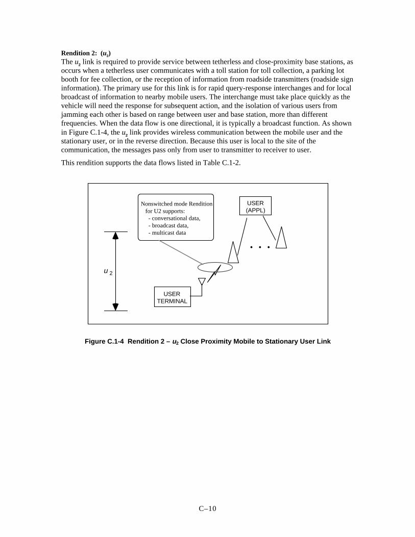
C–10
Rendition 2: (u2)The u2 link is required to provide service between tetherless and close-proximity base stations, asoccurs when a tetherless user communicates with a toll station for toll collection, a parking lotbooth for fee collection, or the reception of information from roadside transmitters (roadside signinformation). The primary use for this link is for rapid query-response interchanges and for localbroadcast of information to nearby mobile users. The interchange must take place quickly as thevehicle will need the response for subsequent action, and the isolation of various users fromjamming each other is based on range between user and base station, more than differentfrequencies. When the data flow is one directional, it is typically a broadcast function. As shownin Figure C.1-4, the u2 link provides wireless communication between the mobile user and thestationary user, or in the reverse direction. Because this user is local to the site of thecommunication, the messages pass only from user to transmitter to receiver to user.
This rendition supports the data flows listed in Table C.1-2.
USER TERMINAL
• • •
USER (APPL)
Nonswitched mode Rendition for U2 supports: - conversational data, - broadcast data, - multicast data
2u
Figure C.1-4 Rendition 2 – u2 Close Proximity Mobile to Stationary User Link

C–11
Table C.1-2 Short Range (Close-Proximity Mobile-Fixed) Wireless Data Flows ( u2)
Flow # Source Source Name Architecture Flow Destination Destination Name Interconnects CommunicationService
Rationale
34 CVS Commercial VehicleSubsystem
on board vehicle data FMS Fleet and FreightManagement
U1t,U2 messaging data Bursty transactions
198 TRMS Transit Management request for vehiclemeasures
TRVS Transit VehicleSubsystem
U1t,U2 Conversational data,messaging data
Bursty data using widearea wirelessor short rang while passing byspecific locations at speeds up to 70mph
201 TRMS Transit Management route assignment TRVS Transit VehicleSubsystem
U1t,U2 messaging data Bursty data using widearea wirelessor short rang while passing byspecific locations at speeds up to 70mph
209 TRVS Transit VehicleSubsystem
transit vehicle conditions TRMS Transit Management U1t,U2 messaging data Bursty data using widearea wirelessor short rang while passing byspecific locations at speeds up to 70mph
213 TRVS Transit VehicleSubsystem
fare and payment status TRMS Transit Management U1t,U2 Conversational data,messaging data
Bursty data using widearea wirelessor short rang while passing byspecific locations at speeds up to 70mph
214 TRVS Transit VehicleSubsystem
transit vehicle passengerand use data
TRMS Transit Management U1t,U2 Conversational data,messaging data
Bursty data using widearea wirelessor short rang while passing byspecific locations at speeds up to 70mph
21 CVCS Commercial VehicleCheck
clearance event record CVS Commercial VehicleSubsystem
U2 Conversational data Short range communication, formoving vehicles when passing byspecific locations at speeds up to 70mph
22 CVCS Commercial VehicleCheck
pass/pull-in CVS Commercial VehicleSubsystem
U2 Conversational data Short range communication, formoving vehicles when passing byspecific locations at speeds up to 70mph
23 CVCS Commercial VehicleCheck
safety inspection record CVS Commercial VehicleSubsystem
U2 Conversational Data Short range communication, formoving vehicles when passing byspecific locations at speeds up to 70mph
24 CVCS Commercial VehicleCheck
screening request CVS Commercial VehicleSubsystem
U2 Conversational data Short range communication, formoving vehicles when passing byspecific locations at speeds up to 70mph
25 CVCS Commercial Vehicle lock tag data request CVS Commercial Vehicle U2 Conversational Data

C–12
Table C.1-2 Short Range (Close-Proximity Mobile-Fixed) Wireless Data Flows ( u2)
Flow # Source Source Name Architecture Flow Destination Destination Name Interconnects CommunicationService
Rationale
Check Subsystem26 CVCS Commercial Vehicle
Checkborder clearance request CVS Commercial Vehicle
SubsystemU2 Conversational data Short range communication, for
moving vehicles when passing byspecific locations at speeds up to 70mph
27 CVCS Commercial VehicleCheck
on-board safety request CVS Commercial VehicleSubsystem
U2 Conversational data Short range communication, formoving vehicles when passing byspecific locations at speeds up to 70mph
28 CVCS Commercial VehicleCheck
border clearance eventrecord
CVS Commercial VehicleSubsystem
U2 Conversational Data Short range communication, formoving vehicles when passing byspecific locations at speeds up to 70mph
29 CVS Commercial VehicleSubsystem
border clearance data CVCS Commercial VehicleCheck
U2 Conversational data Short range communication, formoving vehicles when passing byspecific locations at speeds up to 70mph
30 CVS Commercial VehicleSubsystem
on board safety data CVCS Commercial VehicleCheck
U2 Conversational data Short range communication, formoving vehicles when passing byspecific locations at speeds up to 70mph
31 CVS Commercial VehicleSubsystem
screening data CVCS Commercial VehicleCheck
U2 Conversational data Short range communication, formoving vehicles when passing byspecific locations at speeds up to 70mph
32 CVS Commercial VehicleSubsystem
lock tag data CVCS Commercial VehicleCheck
U2 Conversational Data
61 EVS Emergency VehicleSubsystem
emergency vehiclepreemption request
RS Roadway Subsystem U2 Conversational data Short range bursty datacommunication while in motion,when passing by specific locationsat speeds up to 70 mph
115 PMS Parking Management request tag data VS Vehicle U2 Conversational data Data transfer while in motion, whenpassing the specific locations atspeeds up to 70 mph
116 PMS Parking Management tag update VS Vehicle U2 Conversational data Data transfer while in motion, whenpassing the specific locations atspeeds up to 70 mph
136 RS Roadway Subsystem AHS control data VS Vehicle U2 messaging data Data transfer while in motion, whenpassing the specific locations at
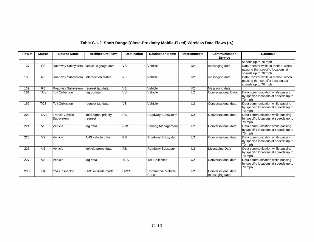
C–13
Table C.1-2 Short Range (Close-Proximity Mobile-Fixed) Wireless Data Flows ( u2)
Flow # Source Source Name Architecture Flow Destination Destination Name Interconnects CommunicationService
Rationale
speeds up to 70 mph137 RS Roadway Subsystem vehicle signage data VS Vehicle U2 messaging data Data transfer while in motion, when
passing the specific locations atspeeds up to 70 mph
138 RS Roadway Subsystem intersection status VS Vehicle U2 messaging data Data transfer while in motion, whenpassing the specific locations atspeeds up to 70 mph
139 RS Roadway Subsystem request tag data VS Vehicle U2 Messaging data161 TCS Toll Collection tag update VS Vehicle U2 Conversational Data Data communication while passing
by specific locations at speeds up to70 mph
162 TCS Toll Collection request tag data VS Vehicle U2 Conversational data Data communication while passingby specific locations at speeds up to70 mph
208 TRVS Transit VehicleSubsystem
local signal priorityrequest
RS Roadway Subsystem U2 Conversational data Data communication while passingby specific locations at speeds up to70 mph
224 VS Vehicle tag data PMS Parking Management U2 Conversational data Data communication while passingby specific locations at speeds up to70 mph
225 VS Vehicle AHS vehicle data RS Roadway Subsystem U2 Conversational data Data communication while passingby specific locations at speeds up to70 mph
226 VS Vehicle vehicle probe data RS Roadway Subsystem U2 Messaging Data Data communication while passingby specific locations at speeds up to70 mph
227 VS Vehicle tag data TCS Toll Collection U2 Conversational data Data communication while passingby specific locations at speeds up to70 mph
236 X10 CVO Inspector CVC override mode CVCS Commercial VehicleCheck
U2 Conversational data,messaging data

C–14
Rendition 3: (u3)
The u3 link is required to provide communication between two (or more) tetherless users, asoccurs in implementing the Automated Highway System (AHS). As shown in Figure C.1-5, theu3 link provides time critical mostly line-of-sight data communication between tetherless users.This is still an area of research and standards for this link are in their infancy. The typical dataflows include:
Source ArchitectureFlow
Destin-ation
CommunicationService
180 VS veh to veh cord X34 Conversational data207 X34 Speed and
HeadwayVS Conversational data
208 X34 veh to veh cord VS Conversational data
USER TERMINAL
Nonswitched mode Rendition for U3 supports: - conversational data, - messaging data, - broadcast data
USER TERMINAL
3u
Figure C.1-5 Rendition 3 – u3, Close Proximity Vehicle-to-Vehicle Connection

C–15
Rendition 4: (w)
The w link mostly makes use of existing public telecommunications services to providecommunication between fixed users. When the fixed users are not local and usage rates are low,the normal telco connection is used, whereas for heavily loaded communications, a dedicatedlink may be installed or leased from the telco. As shown in Figure C.1-6, the w link providesconnection from the user, either through an on-site switch (PBX) or directly ( the dotted boxindicates the switch may not be used) to the public service provider (Internet, PDN or ISDN,etc.), as in the case where access to the Internet was through a cable television service and theentire capacity was used for the single user terminal. The dedicated connection would usuallyonly apply to heavy usage links.
Note that in the figure for the wireline connection, Rendition 4, digital transmission can makeuse of the dedicated line, between single users when high loading is usual, or between switchesto spread its capacity among many users.
This rendition supports the data flows listed in Table C.1-3.
Circuit mode Rendition for W supports: - conversational speech, - conversational data
w
USER TERMINAL
PSTN ISDN Internet PDN
SWITCH
USER TERMINAL
USER TERMINAL
Dedicated line
SWITCH
Packet mode Rendition for W supports: - conversational data - messaging data, - multicast data, - broadcast data
Figure C.1-6 . Rendition 4 – w, The Wireline Connection

C–16
Table C.1-3 Wireline Connection Data Flows ( w)
Flow # Source Source Name Architecture Flow Destination Destination Name Interconnects CommunicationService
Rationale
3 CVAS Commercial VehicleAdministration
CVO database update CVCS Commercial VehicleCheck
W Conversational data,messaging data
4 CVAS Commercial VehicleAdministration
international bordercrossing data
CVCS Commercial VehicleCheck
W messaging data
6 CVAS Commercial VehicleAdministration
compliance review report FMS Fleet and FreightManagement
W messaging data
7 CVAS Commercial VehicleAdministration
activity reports FMS Fleet and FreightManagement
W messaging data
8 CVAS Commercial VehicleAdministration
operational data PS Planning Subsystem W messaging data
9 CVAS Commercial VehicleAdministration
payment request X21 Financial Institution W Conversational data,messaging data
10 CVAS Commercial VehicleAdministration
tax-credentials-feesrequest
X22 GovernmentAdministrators
W messaging data
11 CVAS Commercial VehicleAdministration
credentials and safetyinformation request
X59 Other CVAS W messaging data
12 CVAS Commercial VehicleAdministration
CVAS informationexchange
X59 Other CVAS W messaging data
13 CVAS Commercial VehicleAdministration
violation notification X62 Enforcement Agency W messaging data
14 CVAS Commercial VehicleAdministration
license request X64 DMV W messaging data
15 CVAS Commercial VehicleAdministration
credentials and safetyinformation response
X65 CVO InformationRequestor
W messaging data
16 CVCS Commercial VehicleCheck
credentials informationrequest
CVAS Commercial VehicleAdministration
W Conversational data,messaging data
17 CVCS Commercial VehicleCheck
roadside log update CVAS Commercial VehicleAdministration
W Messaging data
18 CVCS Commercial VehicleCheck
citation and accident data CVAS Commercial VehicleAdministration
W Conversational data,messaging data
19 CVCS Commercial VehicleCheck
safety information request CVAS Commercial VehicleAdministration
W Conversational data,messaging data
20 CVCS Commercial VehicleCheck
international bordercrossing data update
CVAS Commercial VehicleAdministration
W Conversational data,messaging data
35 CVS Commercial VehicleSubsystem
processed cargo data VS Vehicle W messaging data
36 CVS Commercial VehicleSubsystem
lock tag data request X08 Commercial Vehicle W Conversational Data

C–17
Table C.1-3 Wireline Connection Data Flows ( w)
Flow # Source Source Name Architecture Flow Destination Destination Name Interconnects CommunicationService
Rationale
40 EM EmergencyManagement
Hazmat informationrequest
FMS Fleet and FreightManagement
W Conversational data,messaging data
41 EM EmergencyManagement
emergency vehicle routerequest
ISP Information ServiceProvider
W Conversational speech,messaging data
42 EM EmergencyManagement
incident information ISP Information ServiceProvider
W Conversational speech,messaging data
44 EM EmergencyManagement
operational data PS Planning Subsystem W Conversational data,messaging data
46 EM EmergencyManagement
incident information TMS Traffic Management W Conversational data,messaging data
47 EM EmergencyManagement
emergency vehiclegreenwave request
TMS Traffic Management W Conversational dataconversational speec
48 EM EmergencyManagement
incident response status TMS Traffic Management W Conversational data,messaging data
49 EM EmergencyManagement
transit emergencycoordination data
TRMS Transit Management W Conversational data,messaging data
51 EM EmergencyManagement
emergency status X13 E911 or ETS W Conversational dataconversational speec
52 EM EmergencyManagement
map update request X23 Map Update Provider W messaging data
53 EM EmergencyManagement
emergency coordination X30 Other EM W Conversational data,messaging data
54 EMMS EmissionsManagement
operational data PS Planning Subsystem W messaging data
55 EMMS EmissionsManagement
vehicle pollution criteria RS Roadway Subsystem W messaging data
56 EMMS EmissionsManagement
widearea statisticalpollution information
TMS Traffic Management W messaging data
57 EMMS EmissionsManagement
map update request X23 Map Update Provider W messaging data
62 FMS Fleet and FreightManagement
tax filing, audit data CVAS Commercial VehicleAdministration
w messaging data
63 FMS Fleet and FreightManagement
credential application CVAS Commercial VehicleAdministration
W Conversational data,messaging data
64 FMS Fleet and FreightManagement
information request CVAS Commercial VehicleAdministration
W Conversational data,messaging data
66 FMS Fleet and FreightManagement
Hazmat information EM EmergencyManagement
W Conversational data,messaging data

C–18
Table C.1-3 Wireline Connection Data Flows ( w)
Flow # Source Source Name Architecture Flow Destination Destination Name Interconnects CommunicationService
Rationale
67 FMS Fleet and FreightManagement
route request ISP Information ServiceProvider
W Conversational data,messaging data
68 FMS Fleet and FreightManagement
intermod CVO coord X01 Intermodal FreightShipper
W messaging data
69 FMS Fleet and FreightManagement
intermod CVO coord X60 Intermodal FreightDepot
W messaging data
70 ISP Information ServiceProvider
emergency vehicle route EM EmergencyManagement
W Conversational speech,messaging data
71 ISP Information ServiceProvider
incident informationrequest
EM EmergencyManagement
W Conversational speech,messaging data
72 ISP Information ServiceProvider
route plan FMS Fleet and FreightManagement
W messaging data
76 ISP Information ServiceProvider
parking lot data request PMS Parking Management W messaging data
77 ISP Information ServiceProvider
parking reservationsrequest
PMS Parking Management W messaging data
78 ISP Information ServiceProvider
road network use PS Planning Subsystem W messaging data
79 ISP Information ServiceProvider
traveler information RTS Remote TravelerSupport
W Broadcastdata,Multicast data
81 ISP Information ServiceProvider
trip plan RTS Remote TravelerSupport
W Conversational Data
82 ISP Information ServiceProvider
request for toll schedules TAS Toll Administration W messaging data
83 ISP Information ServiceProvider
incident notification TMS Traffic Management W Conversational Data
84 ISP Information ServiceProvider
request for trafficinformation
TMS Traffic Management W messaging data
85 ISP Information ServiceProvider
logged route plan TMS Traffic Management W Conversational data,Messaging data
86 ISP Information ServiceProvider
road network use TMS Traffic Management W messaging data
87 ISP Information ServiceProvider
transit information request TRMS Transit Management W messaging data
88 ISP Information ServiceProvider
selected routes TRMS Transit Management W Conversational data,Messaging data
89 ISP Information ServiceProvider
demand responsivetransit request
TRMS Transit Management W messaging data

C–19
Table C.1-3 Wireline Connection Data Flows ( w)
Flow # Source Source Name Architecture Flow Destination Destination Name Interconnects CommunicationService
Rationale
93 ISP Information ServiceProvider
intermodal information X02 IntermodalTransportationService Provider
W messaging data
94 ISP Information ServiceProvider
payment request X21 Financial Institution W Conversational data,messaging data
95 ISP Information ServiceProvider
map update request X23 Map Update Provider W messaging data
96 ISP Information ServiceProvider
travel service reservation X24 Yellow PagesService Providers
W messaging data
97 ISP Information ServiceProvider
traffic information X27 Media W messaging data
98 ISP Information ServiceProvider
incident information X27 Media W messaging data
99 ISP Information ServiceProvider
traffic information X28 Media Operator W messagingdata,Broadcast data,Multicast
100 ISP Information ServiceProvider
incident information X28 Media Operator W messaging data
101 ISP Information ServiceProvider
ISP coord X31 Other ISP W messaging data
109 PMS Parking Management parking lot reservationconfirmation
ISP Information ServiceProvider
W messaging data
110 PMS Parking Management parking availability ISP Information ServiceProvider
W messaging data
111 PMS Parking Management operational data PS Planning Subsystem W messaging data112 PMS Parking Management demand management
price change responseTMS Traffic Management W messaging data
113 PMS Parking Management parking availability TMS Traffic Management W messaging data114 PMS Parking Management transit parking
coordinationTRMS Transit Management W Messaging data
117 PMS Parking Management payment request X21 Financial Institution W Conversational data,messaging data
118 PMS Parking Management parking status X36 Parking Operator W messaging data119 PMS Parking Management parking availability X37 Parking Service
ProviderW messaging data
120 PMS Parking Management violation notification X62 Enforcement Agency W messaging data121 PMS Parking Management license request X64 DMV W Messaging data122 PS Planning Subsystem planning data TMS Traffic Management W messaging data

C–20
Table C.1-3 Wireline Connection Data Flows ( w)
Flow # Source Source Name Architecture Flow Destination Destination Name Interconnects CommunicationService
Rationale
123 PS Planning Subsystem map update request X23 Map Update Provider W Messaging data124 PS Planning Subsystem planning data X25 Transportation
PlannersW messaging data
125 RS Roadway Subsystem pollution data EMMS EmissionsManagement
W messaging data
126 RS Roadway Subsystem fault reports TMS Traffic Management W Conversational data,messaging data
127 RS Roadway Subsystem request for right of way TMS Traffic Management W Conversational Data128 RS Roadway Subsystem vehicle probe data TMS Traffic Management W messaging data129 RS Roadway Subsystem AHS status TMS Traffic Management W messaging data130 RS Roadway Subsystem incident data TMS Traffic Management W messaging data131 RS Roadway Subsystem freeway control status TMS Traffic Management w messaging data132 RS Roadway Subsystem signal control status TMS Traffic Management W messaging data133 RS Roadway Subsystem HOV data TMS Traffic Management W Messaging data134 RS Roadway Subsystem signal priority request TMS Traffic Management W messaging data135 RS Roadway Subsystem local traffic flow TMS Traffic Management W messaging data140 RS Roadway Subsystem grant right of way and/or
stop trafficX29 Multimodal Crossings W Conversational data,
messaging data142 RTS Remote Traveler
Supportyellow pages request ISP Information Service
ProviderW Conversational data,
Messaging Data143 RTS Remote Traveler
Supporttrip request ISP Information Service
ProviderW Conversational Data
144 RTS Remote TravelerSupport
traveler informationrequest
ISP Information ServiceProvider
W messaging data
145 RTS Remote TravelerSupport
demand responsivetransit request
ISP Information ServiceProvider
W messaging data
146 RTS Remote TravelerSupport
emergency notification TRMS Transit Management W Conversational data,Messaging Data
147 RTS Remote TravelerSupport
transit request TRMS Transit Management W messaging data
148 RTS Remote TravelerSupport
traveler informationrequest
TRMS Transit Management W messaging data
149 RTS Remote TravelerSupport
map update request X23 Map Update Provider W messaging data
150 TAS Toll Administration toll schedules ISP Information ServiceProvider
W messaging data
151 TAS Toll Administration operational data PS Planning Subsystem W messaging data152 TAS Toll Administration toll instructions TCS Toll Collection W messaging data
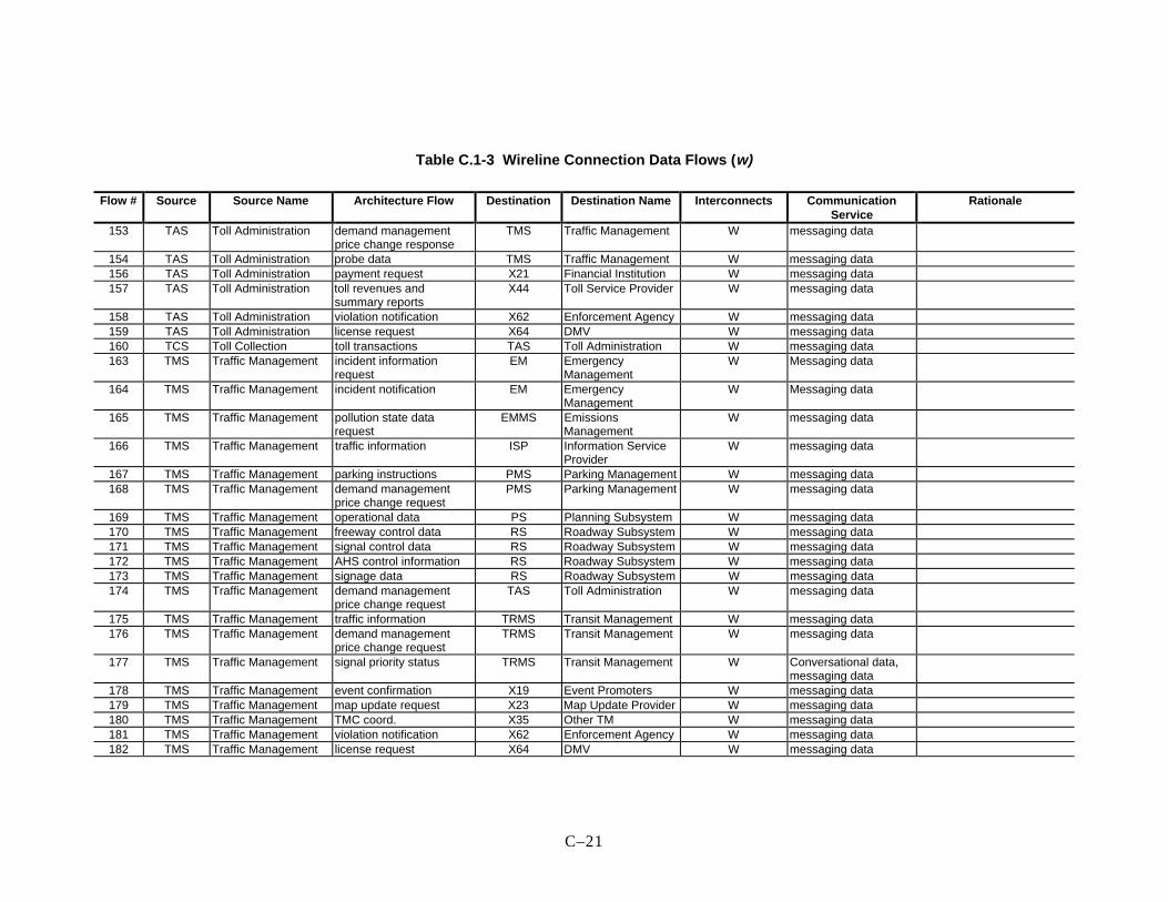
C–21
Table C.1-3 Wireline Connection Data Flows ( w)
Flow # Source Source Name Architecture Flow Destination Destination Name Interconnects CommunicationService
Rationale
153 TAS Toll Administration demand managementprice change response
TMS Traffic Management W messaging data
154 TAS Toll Administration probe data TMS Traffic Management W messaging data156 TAS Toll Administration payment request X21 Financial Institution W messaging data157 TAS Toll Administration toll revenues and
summary reportsX44 Toll Service Provider W messaging data
158 TAS Toll Administration violation notification X62 Enforcement Agency W messaging data159 TAS Toll Administration license request X64 DMV W messaging data160 TCS Toll Collection toll transactions TAS Toll Administration W messaging data163 TMS Traffic Management incident information
requestEM Emergency
ManagementW Messaging data
164 TMS Traffic Management incident notification EM EmergencyManagement
W Messaging data
165 TMS Traffic Management pollution state datarequest
EMMS EmissionsManagement
W messaging data
166 TMS Traffic Management traffic information ISP Information ServiceProvider
W messaging data
167 TMS Traffic Management parking instructions PMS Parking Management W messaging data168 TMS Traffic Management demand management
price change requestPMS Parking Management W messaging data
169 TMS Traffic Management operational data PS Planning Subsystem W messaging data170 TMS Traffic Management freeway control data RS Roadway Subsystem W messaging data171 TMS Traffic Management signal control data RS Roadway Subsystem W messaging data172 TMS Traffic Management AHS control information RS Roadway Subsystem W messaging data173 TMS Traffic Management signage data RS Roadway Subsystem W messaging data174 TMS Traffic Management demand management
price change requestTAS Toll Administration W messaging data
175 TMS Traffic Management traffic information TRMS Transit Management W messaging data176 TMS Traffic Management demand management
price change requestTRMS Transit Management W messaging data
177 TMS Traffic Management signal priority status TRMS Transit Management W Conversational data,messaging data
178 TMS Traffic Management event confirmation X19 Event Promoters W messaging data179 TMS Traffic Management map update request X23 Map Update Provider W messaging data180 TMS Traffic Management TMC coord. X35 Other TM W messaging data181 TMS Traffic Management violation notification X62 Enforcement Agency W messaging data182 TMS Traffic Management license request X64 DMV W messaging data
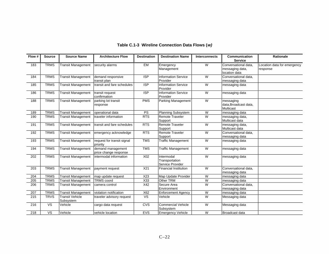
C–22
Table C.1-3 Wireline Connection Data Flows ( w)
Flow # Source Source Name Architecture Flow Destination Destination Name Interconnects CommunicationService
Rationale
183 TRMS Transit Management security alarms EM EmergencyManagement
W Conversational data,messaging data,location data
Location data for emergencyresponse
184 TRMS Transit Management demand responsivetransit plan
ISP Information ServiceProvider
W Conversational data,messaging data
185 TRMS Transit Management transit and fare schedules ISP Information ServiceProvider
W messaging data
186 TRMS Transit Management transit requestconfirmation
ISP Information ServiceProvider
W messaging data
188 TRMS Transit Management parking lot transitresponse
PMS Parking Management W messagingdata,Broadcast data,Multicast
189 TRMS Transit Management operational data PS Planning Subsystem W messaging data190 TRMS Transit Management traveler information RTS Remote Traveler
SupportW messaging data,
Multicast data191 TRMS Transit Management transit and fare schedules RTS Remote Traveler
SupportW messaging data,
Multicast data192 TRMS Transit Management emergency acknowledge RTS Remote Traveler
SupportW Conversational data,
messaging data193 TRMS Transit Management request for transit signal
priorityTMS Traffic Management W messaging data
194 TRMS Transit Management demand managementprice change response
TMS Traffic Management W messaging data
202 TRMS Transit Management intermodal information X02 IntermodalTransportationService Provider
W messaging data
203 TRMS Transit Management payment request X21 Financial Institution W Conversational data,messaging data
204 TRMS Transit Management map update request X23 Map Update Provider W messaging data205 TRMS Transit Management TRMS coord X33 Other TRM W messaging data206 TRMS Transit Management camera control X42 Secure Area
EnvironmentW Conversational data,
messaging data207 TRMS Transit Management violation notification X62 Enforcement Agency W messaging data215 TRVS Transit Vehicle
Subsystemtraveler advisory request VS Vehicle W Messaging data
216 VS Vehicle cargo data request CVS Commercial VehicleSubsystem
W Messaging data
218 VS Vehicle vehicle location EVS Emergency Vehicle W Broadcast data

C–23
Table C.1-3 Wireline Connection Data Flows ( w)
Flow # Source Source Name Architecture Flow Destination Destination Name Interconnects CommunicationService
Rationale
Subsystem228 VS Vehicle vehicle location TRVS Transit Vehicle
SubsystemW Broadcast data
229 VS Vehicle vehicle control X03 Basic Vehicle W Conversational Data231 X01 Intermodal Freight
Shipperintermod CVO coord FMS Fleet and Freight
ManagementW messaging data
232 X02 IntermodalTransportationService Provider
intermodal information ISP Information ServiceProvider
W messaging data
233 X02 IntermodalTransportationService Provider
intermodal information TRMS Transit Management W messaging data
234 X03 Basic Vehicle vehicle measures VS Vehicle W Broadcast data235 X08 Commercial Vehicle vehicle measures CVS Commercial Vehicle
SubsystemW Broadcast data
237 X13 E911 or ETS incident information EM EmergencyManagement
W Conversational dataconversational speec,location data
Location data for emergencyresponse
238 X19 Event Promoters event plans TMS Traffic Management W messaging data,Multicast data
239 X21 Financial Institution transaction status CVAS Commercial VehicleAdministration
W Conversational data,messaging data
240 X21 Financial Institution transaction status ISP Information ServiceProvider
W Conversational data,messaging data
241 X21 Financial Institution transaction status PMS Parking Management W Conversational data,messaging data
242 X21 Financial Institution transaction status TAS Toll Administration W Conversational data,messaging data
243 X21 Financial Institution transaction status TRMS Transit Management W Conversational data,messaging data
244 X22 GovernmentAdministrators
regulations CVAS Commercial VehicleAdministration
W messaging data,Multicast data
245 X23 Map Update Provider map updates EM EmergencyManagement
W messaging data,Multicast data
246 X23 Map Update Provider map updates EMMS EmissionsManagement
W messaging data
247 X23 Map Update Provider map updates ISP Information ServiceProvider
W messaging data,Multicast data

C–24
Table C.1-3 Wireline Connection Data Flows ( w)
Flow # Source Source Name Architecture Flow Destination Destination Name Interconnects CommunicationService
Rationale
249 X23 Map Update Provider map updates PS Planning Subsystem W messagingdata,Broadcast data,Multicast
250 X23 Map Update Provider map updates RTS Remote TravelerSupport
W messaging data
251 X23 Map Update Provider map updates TMS Traffic Management W messaging data,Multicast data
252 X23 Map Update Provider map updates TRMS Transit Management W messaging data,Multicast data
254 X24 Yellow Pages ServiceProviders
travel service info ISP Information ServiceProvider
W messaging data
255 X25 TransportationPlanners
planning data PS Planning Subsystem W messaging data
256 X27 Media external reports ISP Information ServiceProvider
W messaging data,Multicast data
257 X28 Media Operator incident notification ISP Information ServiceProvider
W messagingdata,Broadcast data,Multicast
258 X29 Multimodal Crossings right of way preemptionrequest
RS Roadway Subsystem W Conversational data,messaging data
259 X29 Multimodal Crossings request for right of way RS Roadway Subsystem W Conversational data,messaging data
260 X30 Other EM emergency coordination EM EmergencyManagement
W Conversational data,messaging data
261 X31 Other ISP ISP coord ISP Information ServiceProvider
W messaging data
262 X33 Other TRM TRMS coord TRMS Transit Management W messaging data263 X35 Other TM TMC coord. TMS Traffic Management W messaging data264 X37 Parking Service
Providerrequest for performancedata
PMS Parking Management W messaging data
265 X51 Transit Vehicle vehicle measures TRVS Transit VehicleSubsystem
W Broadcast data
266 X58 Weather Service weather information ISP Information ServiceProvider
W messagingdata,Broadcast data,Multicast
267 X58 Weather Service weather information TMS Traffic Management W messagingdata,Broadcast data,Multicast

C–25
Table C.1-3 Wireline Connection Data Flows ( w)
Flow # Source Source Name Architecture Flow Destination Destination Name Interconnects CommunicationService
Rationale
268 X59 Other CVAS CVAS informationexchange
CVAS Commercial VehicleAdministration
W messaging data
269 X59 Other CVAS credentials and safetyinformation response
CVAS Commercial VehicleAdministration
W messaging data
270 X60 Intermodal FreightDepot
intermod CVO coord FMS Fleet and FreightManagement
W messaging data
271 X64 DMV registration CVAS Commercial VehicleAdministration
W messaging data
272 X64 DMV vehicle characteristics PMS Parking Management W Messaging data273 X64 DMV registration TAS Toll Administration W messaging data274 X64 DMV registration TMS Traffic Management W messaging data275 X65 CVO Information
Requestorcredentials and safetyinformation request
CVAS Commercial VehicleAdministration
W messaging data
73 ISP Information ServiceProvider
broadcast information PIAS Personal InformationAccess
W,U1b messagingdata,Broadcast data,Multicast
Free services & services thatrequire subscription
1 CVAS Commercial VehicleAdministration
credentials information CVCS Commercial VehicleCheck
W,U1t Conversational data,messaging data
The CVAS could be atransportable entity. Sometranactions may need realtime support
2 CVAS Commercial VehicleAdministration
safety information CVCS Commercial VehicleCheck
W,U1t Conversational data,messaging data
5 CVAS Commercial VehicleAdministration
electronic credentials FMS Fleet and FreightManagement
W,U1t messaging data The CVAS could be atransportable entity.
43 EM EmergencyManagement
emergency acknowledge PIAS Personal InformationAccess
W,U1t Conversational data,messaging data
Wide area communication toPDA
45 EM EmergencyManagement
emergency acknowledge RTS Remote TravelerSupport
W,U1t Conversational speech,messaging data
Wide area wirelesscommunication totransportable units
74 ISP Information ServiceProvider
trip plan PIAS Personal InformationAccess
W,U1t Conversational data,Messaging data
Bursty data
75 ISP Information ServiceProvider
traveler information PIAS Personal InformationAccess
W,U1t Broadcastdata,Multicast data
Bursty data upon request.Bursty or continuoustransmission for one-waysystems. Free services andservices that requiresubscription.
103 PIAS Personal Information traveler information ISP Information Service W,U1t messaging data Bursty messages, Wireless

C–26
Table C.1-3 Wireline Connection Data Flows ( w)
Flow # Source Source Name Architecture Flow Destination Destination Name Interconnects CommunicationService
Rationale
Access request Provider to PDA. Location data forvalue added services.
104 PIAS Personal InformationAccess
trip request ISP Information ServiceProvider
W,U1t Conversational Data,Messaging data
Bursty messages, Wirelessto PDA
105 PIAS Personal InformationAccess
trip confirmation ISP Information ServiceProvider
W,U1t Conversational Data,Messaging data
Bursty messages. Wirelessto PDA
106 PIAS Personal InformationAccess
yellow pages request ISP Information ServiceProvider
W,U1t Conversational Data,Messaging data
Bursty messages, Wirelessto PDA
108 PIAS Personal InformationAccess
map update request X23 Map Update Provider W,U1t messaging data Service on request orservices by subscription
141 RTS Remote TravelerSupport
emergency notification EM EmergencyManagement
W,U1t Conversational speech,messaging data,location data
RTS can be a transportableunit. Location dataemergency response.
187 TRMS Transit Management demand responsivetransit route
PIAS Personal InformationAccess
W,U1t messaging data Bursty data
248 X23 Map Update Provider map updates PIAS Personal InformationAccess
W,U1t messaging data,Multicast data
Service on request or bysubscription

C–27
C.2 Applicable Technologies Mapped to the Renditions
The task here is to identify applicable technologies which will support the Level 0 Rendition.This requires assessing the technologies presented in Appendix D, and then mapping them ontothe Rendition Level 0 diagram as shown in Figure C.2-1. Evaluation of these technologies yieldsthe Architecture Interconnect Specifications. A host of existing and emerging technologiesapplicable to ITS are identified in Appendix D. This assessment covers the candidatecommunication technologies depicted in Figure C.2-1.
The wireline technologies are typically provided by the local Telco and other service providers,although private networks are sometimes used when the loading is high enough to justify thecost. Even then, lines are often leased from the local Telco. The choice between the differentservices (PSTN, ISDN, IP, PDN) will be based almost exclusively on cost. As the competition toprovide these services continues, it will be easy to switch from one to the other as the datatransmission loads change and new services are offered.
As an illustrative example, a set of communication technologies that are applicable to providesome or all of the services identified in the AIDs for the u1t link are listed in the highlighted boxin Figure C.2-2. This figure shows the list of technologies superimposed on the u1t Level 1rendition.
w
User
u
Useru
User
Central Office
Base Station
Base Station
u
Rendition 3
Rendition 2
Rendition 1
Rendition 4
U1t Interface: • CDPD • IS-95 Packet Data • PCS Packet Data • MSAT Packet Data • ESMR Packet Data
U3 Interface: • Active RF
1
2
3
w, u1
w
U2 Interface: • Active RF • Recommendadoption of theindustry's ETTMstandard
User
User
W Interface: PDN: • X.25 • Full-period Interconnection IP: • Internet, OSInet • Full-period Interconnection PSTN, ISDN: • Telco Private Network: • SONET, ATM
U1b Interface - FM Subcarrier - Paging
Figure C.2-1 Technology Mapping onto Level 0 Rendition

C–28
WIRELESS CONTROLLER
OTHER PACKET SWITCH
BASE STATIONs• • •
FIXED NETWORK
OAM&P
USER TERMINAL • • •
MODEM BANK
PACKET SWITCH
CIRCUIT SWITCH
OTHER CIRCUIT SWITCH
USER TERMINAL
USER TERMINAL
T1
Packet mode Rendition for U1t supports: - messaging data, - multicast data,
Circuit mode Rendition for U1t supports: - conversational speech, - conversational data
U1t Interface: • CDPD • IS-95 Packet Data • PCS Packet Data • MSAT Packet Data • ESMR Packet Data
1u
Figure C.2-2 Candidate Technologies for Rendition Level 1 – Two-Way Wide Area WirelessLink

D–1
APPENDIX D TECHNOLOGY ASSESSMENT SOURCES
This appendix provides a list of technical sources and the URL’s of web sites that were used toobtain information on the systems evaluated in Section 7.5. This information is intended tofacilitate more in-depth study of the systems and to provide up-to-date technical, availability, andprice information. Whenever possible, information for direct contact with the companiesinvolved will also be provided. As a general rule, ITS America’s World Wide Web site,http://www.itsa.org/, is a major source of information, however it is restricted to ITS Americamembership.
D.1 Wireless
Wireless has seen in recent times an explosion of new books, making it almost impossible to track thewealth of information now available. As a compromise, reference will be made only to those works thatendure the test of time, though still providing enough timely information to be useful.
D.1.1 MAN’s
Due to their proprietary nature, there is little existing information on MAN’s, especially on those usingthe ISM band. Therefore, only WWW references can be provided at this time.
Company URLMetricom, Inc.980 University AvenueLos Gatos, CA 95030(408) 399-8200
http://www.metricom.com/metricom.html
Tetherless Access Ltd.930 E. Arques Ave.Sunnyvale CA 94086(408) 523-8000
http://www.tetherless.net/home.html

D–2
D.1.2 Land Mobile Systems
General Sources:
1. Wireless Information Networks, K. Pahlavan, A. Levesque, John Wiley & Sons, 1995
2. Wireless Data Networking, N.J. Muller, Artech House, 1995
3. Wireless Personal Communications - The Future of Talk, R. Schneiderman, IEEE Press, 1994
4. Cellular Radio Systems, D.M. Balston, R.C.V. Macario, Eds., Artech House, 1993
5. Mobile Information Systems, J. Walker, Ed., Artech House, 1990
GSM Sources:
1. The GSM System for Mobile Communications, M. Mouly, M.-B. Pautet, self-published, 1992
2. An Introduction to GSM, S.M. Redl, M.K. Weber, M.W. Oliphant, Artech House, 1995
3. Mobile Radio Communications, R. Steele, Ed., Pentech Press Publishers, London, 1992
WWW sites and contacts:
Company URLOmnipoint Corporation1365 Garden of the Gods RoadColorado Springs, CO 80907(719) 548-1200
http://www.omnipoint.com/
Northern Telecom Ltd. http://www.nortel.com/english/wireless/omnipnt.html
RAM Mobile DataWoodbridge, NJ908-602-5500
http://www.ram-wireless.com/
BellSouth Mobile Data, Inc.1100 Peachtree Street, NE, Room 5D09Atlanta, GA 30309-4599(404) 249-4744
http://www.data-mobile.com/
Ericsson Mobile Communications AB Mobitex
http://www.ericsson.com/mobitex/
http://www.ericson.nl/EPI/BR/2mobitex.html
D-AMPS 1900
http://www.ericsson.com/systems/D-AMPS_1900/
ARDISLincolnshire, IL708-913-1215
http://www.ardis.com/ardis_hp/website2.htm
IBM Wireless700 Park Office Road, Highway 54Building 662Research Triangle Park, NC 27709(919) 543-7708
http://www.raleigh.ibm.com/cel/celinfo.html
Nextel Communications Inc.Rutherford, NJ
Geotek Communications Inc.20 Craig Road, Montvale, NJ 07645(201) 930-9305
http://www.geotek.com/
SkyTel Corp. http://www.skytel.com/
http://www.skytel.com/Products/2way/

D–3
Motorola http://www.mot.com/MIMS/WDG/
http://www.mot.com/MIMS/PPG/org/amg/products/tango/
QUALCOMM Incorporated6455 Lusk BoulevardSan Diego, CA 92121-2779(619) 587-1121
http://www.qualcomm.com/QualHome.html/
CDPD Sources:
Company URLIBM Corp. Wireless Headquarters http://www.raleigh.ibm.com/cel/celinfo.html
AT&T Wireless Services http://www.airdata.com/index.html
CDPD Forum Inc. http://www.cdpd.org/
Northern Telecom Ltd. http://www.nortel.com/english/wireless/cdpd_net.html
Pacific Communication Sciences Inc. http://www.pcsi.com/html/pr_cdpd.html
Tellabs Wireless Inc. http://steinbrecher.com/architecture.html
http://steinbrecher.com/compare.html
Rockwell International Corp. http://www.nb.rockwell.com/pb/cdpd.html
http://www.nb.rockwell.com/wcd/wireless.html
Sierra Wireless Inc. http://www.sierrawireless.ca/products.htm
Cincinnati Microwave http://www.cnmw.com/
http://www.cnmw.com/product/cdpd/cdpdhm.htm
Motorola http://www.mot.com/MIMS/WDG/Technology/CelTAC/
CDPD Service Providers
Company Service Name Deployed
Ameritech Cellular Services Hoffman Estates, IL 708-248-2000
WirelessPacket DataService
Chicago, Detroit/Ann Arbor, Gary,IN, Cincinnati, Columbus,OH, Milwaukee
Bell Atlantic Mobile Corp. Bedminster, NJ 908-306-7000
Airbridge PacketService
Charlotte, NC; New London,CT; Northern New Jersey; Philadelphia;Phoenix; Pittsburgh; Washington,DC/ Baltimore;Hartford, CT
Comcast Cellular Communications Inc. Wayne, PA 610-995-5000
Philadelphia; Delaware; New Jersey
GTE Mobilnet Atlanta, GA 404-391-8000
CDPD Service Houston, San Francisco, San Jose/ Oakland, Cleveland, Indianapolis,Memphis, Nashville, Tampa/ St. Petersburg
AT&T Wireless(ex-McCaw Cellular Communications Inc.) Kirkland, WA 206-803-4000
Airdata Dallas, Las Vegas, Miami, New York, Seattle, Denver, Jacksonville,Orlando, Tampa/ St. Petersburg, West Palm Beach, Kansas City,Minneapolis, Oklahoma City, Pittsburgh, Portland, OR, Sacramento,Salt Lake City, San Antonio, San Jose
Nynex MobileCommunications Co.Orangeburg, NY914-365-7200
Boston; New York
Sprint Cellular Co. Chicago 312-399-2275
New Mexico; Las Vegas, Greensboro/Winston-Salem, Norfolk

D–4
GSM/PCS 1900 Sources, and Service Providers
Company URLVODAFONE http://www.vodafone.co.uk/n3/index/indhome
Northern Telecom Ltd. http://www.nortel.com/english/wireless/pcs_1900.html
Sprint Spectrum L.P. http://www.sprint.com/home/product/spectrum.html
D.1.3 Satellite Mobile Systems
In compiling the information on Satellite systems, two major sources were used:
1. Satellite Communication Systems - Mobile and Fixed Services, M.J. Miller, B. Vucetic, L. Berry,Eds., Kluwer Academic Publs., 1993
2. Digital Satellite Communications Systems and Technologies - Military and Civil Applications, A.N.Ince, Ed., Kluwer Academic Publs., 1992
In addition, extensive use was made of the WWW to track the most recent information on the proposedsystems and to obtain the graphics relating to the systems’ characteristics, mainly their orbits andcoverage.
Company URLIridium http://leonardo.jpl.nasa.gov/msl/QuickLooks/iridiumQL.htmlTeledesic http://leonardo.jpl.nasa.gov/msl/QuickLooks/teledesicQL.htmlOdyssey http://leonardo.jpl.nasa.gov/msl/QuickLooks/odysseyQL.html
ICO Global Communications http://www.i-co.co.uk/index-page.html
Orbcomm http://leonardo.jpl.nasa.gov/msl/QuickLooks/orbcommQL.html
Skycell http://www.azstarnet.com/public/commerce/satellite/
MSAT http://www.radiosat.com/radiostar/msat.htm
OmniTRACS http://www.qualcomm.com/ProdTech/Omni/
INMARSAT http://www.inmarsat.org/inmarsat/
COMSAT http://www.comsat.com/
GPS http://leonardo.jpl.nasa.gov/msl/Programs/gps.html
DGPS http://www.inforamp.net/~pinpoint/
Differential Corrections Inc.10121 Miller AveCupertino, CA 95014408-446-8350
http://www.dgps.com/
Omnistar, Inc.8200 WestglenHouston, TX 77063713-785-5850
http://www.omnistar.com/
Glonass http://leonardo.jpl.nasa.gov/msl/QuickLooks/glonassQL.html
Mike’s Spacecraft Library (@ JPL) http://leonardo.jpl.nasa.gov/msl/home.html

D–5
D.1.4 Meteor Burst Systems
Main sources:
1. Meteor Burst Communications - Theory and Practice, D.L. Schilling, Ed., John Wiley & Sons, 1993
2. Meteor Burst Communications, J.Z. Schanker, Artech House, 1990
D.1.5 Broadcast Systems
An interesting article appeared recently in the IEEE Spectrum Magazine, covering most aspects of digitalbroadcasting:
1. “Broadcasting with Digital Audio”, Robert Braham, Ed., IEEE Spectrum, March 1996
D.1.5.1 FM Subcarrier
Similar pages exist for other cities in the country:
City URLSan Diego, CA http://www.scubed.com/caltrans/sd/big_map.shtmlLos Angeles, CA http://www.scubed.com/caltrans/la/la_big_map.shtmlSeattle, WA http://www.wsdot.wa.gov/regions/northwest/NWFLOW/Houston, TX http://herman.tamu.edu/traffic.htmlChicago, IL http://www.ai.eecs.uic.edu/GCM/CongestionMap.html
D.1.5.2 DAB
Company URLEuroDAB Newsletter http://www.ebu.ch/dep_tech/eurodab.htmlDigital Radio Research Inc. (DRRI) http://radioworks.cbc.ca/radio/digital-radio/drri.htmlUSA Digital Radio http://www.usadr.com/techieam.html
D.1.6 Short-Range Communications
ITS America’s World Wide Web site, http://www.itsa.org/ is the main source of short-rangecommunications information, since it maintains a data base of all related information.
D.1.6.1 DSRC Communications
Company Home PageHughes http://www.hughes.com/

D–6
D.1.6.2 Vehicle-to-Vehicle Communications
AHS is still quite a new area, and information of interest can be found almost exclusively in trademagazines and in academic publications. A good example of the latter is the IVHS Journal, now ITSJournal, where a few papers have focused on this issue.
D.2 Wireline Communications
Sources in this area abound. Here are just a few ones that we think are more appropriate given theiremphasis on performance:
1. Advances in Telecommunications Networks, W.S. Lee, D.C. Brown, Artech House, 1995
2. FDDI and FDDI-II: Architecture, Protocols, and Performance, B. Albert, A.P. Jayasumana, ArtechHouse, 1994
3. SMDS: Wide-Area Data Networking with Switched Multi-megabit Data Service, R.W. Klessig, K.Tesink, Prentice-Hall, 1995
4. Asynchronous Transfer Mode Networks: Performance Issues, R.O. Onvural, Artech House, 1994
As for service contacts, all RBOC’s and major telecommunication companies offer wireline services ofall kinds.

E–1
APPENDIX E POTENTIAL USERS ACCORDING TO
USER SERVICE GROUP
In order to enhance the understanding of the data loads generated by ITS services, the analyseswere performed for seven distinct user service groups, each with its own population, message set,peak period definition, and message frequency of use. The user service groups include privatevehicles, CVO-Local vehicles, CVO-long haul vehicles, travelers (PIAS users), transitmanagement, emergency management, and probes.
The number of potential users that might buy a service was determined for each of the ninescenarios through the use of national statistics. The analysis used in the derivation is shownbelow, using the 1997 Urbansville scenario as an example. The same derivation was used foreach of the other eight scenarios, working from the total population and number of householdvehicles of the scenario region in that time frame. The theory is that the number of vehicles of alltypes can be related to the population, as long as the scenario regions all have the same servicesavailable. The lack of a particular service (e.g. fixed route transit in the rural scenario) washandled later in the data loading models with the lack of an entry in the database table of marketpackages of services for that scenario, preventing messages related to that service from beingincluded in the message set for that scenario.
In the case of the Thruville scenario, the added traffic traveling completely through the entirescenario region must be added to the models shown here. This was accomplished by increasingthe number of private vehicles and CVO long haul vehicles shown here by one-third. The otheruser service groups do not travel through the scenario region by definition.
The number of potential users was derived for the peak period defined for that particular userservice group. The number of potential users for the off-peak period was then defined as afraction of the peak period number.

E–2
E.1 Private Vehicle Service Group Users – Urbansville, 1997
The peak period for this user service group is defined as the two, three-hour periods of 6 am to 9am, and 4 PM to 7 PM. This two-peak model may not be very pronounced over the traffic whichoccurs between the peaks in many urban areas, but the peaks are present. The number ofhousehold vehicles in the Urbansville region is defined in the Urbansville Scenario Guide for thefive-year time frame as 1,688,9701. The average daily number of miles driven per householdvehicle in the Urbansville region was derived from the average number of household vehiclemiles traveled per year in the US (1.4096 x 10¹²)2 divided by the total number of householdvehicles in the US (1.6522 x 10⁸)3. This result (8531.6 miles per year) is divided by 365 to obtainthe average household vehicle miles traveled per day (23.374). There is little error in theassumption that the miles driven are equal for every day of the week. The distribution of persontrips by day of the week shows little variation between week days and weekend days4. The dailyhousehold vehicle miles traveled (23.374) is multiplied by the number of household vehicles inthe Urbansville region (1,688,970) to obtain the Daily Vehicles Miles Traveled (DVMT) forUrbansville.
DVMT = 39,478,000 miles
Since we are principally interested in the peak period traffic, we must then obtain the DVMT inthe peak period, consisting of the two, three-hour periods. The fraction of traffic found in onestudy to consistently occur during the peak periods was 45%5. The number of weekday trips inthe peak periods was found by survey to be 41.3% of the daily trips6. A CALTRANS study foundthat the traffic counts during the peak periods were 37.6% of the daily traffic on their freewaysystem7. Using an rounded up average fraction of 42%, and multiplying DVMT by that peak-period fraction (0.42), results in the peak-period DVMT (PDVMT):
PDVMT = 16,700,000 miles
Dividing PDVMT by the average trip length during the peak period will result in the number oftrips during the peak period. The trip length used is 11 miles8. Since 95% of the household travel
1 Urban Scenario Guide, Urbansville, Phase II, March 13, 1995.
2 Summary of Travel Trends, 1990 National Personal Transportation Survey, Center for TransportationAnalysis, Energy Division, Oak Ridge National Laboratory, Oak Ridge TN, 1993, page 6.
3 Summary of Travel Trends, 1990 National Personal Transportation Survey, Center for TransportationAnalysis, Energy Division, Oak Ridge National Laboratory, Oak Ridge TN, 1993, page 6.
4 NPTS Databook, National Personal Transportation Survey, Volume I, Center for Transportation Analysis,Energy Division, Oak Ridge National Laboratory, Oak Ridge TN, 1993, page 4-103.
5 Hanks, J. W., and T. J. Lomax, Roadway Congestion in Major Urban Areas 1982 to 1988, TexasTransportation Institute, College Station, Texas, 1990, page D-5.
6 NPTS Databook, National Personal Transportation Survey, Volume I, Center for Transportation Analysis,Energy Division, Oak Ridge National Laboratory, Oak Ridge TN, 1993, page 4-108.
7 Perrin, C., California Department of Transportation, private communications, 1994.
8 National Transportation Statistics, Annual Report, September 1993, Historical Compendium, 1960-1992,Department of Transportation, 1993, page 198.

E–3
during the AM commute time is commuter travel9, and the average trip length for all trips is 9.0miles10, there is little error in using the 11 mile trip length for all trips in the peak periods. Theresulting number of peak-period trips in the peak period defined (consisting of two, three-hourperiods) is 1,520,000 trips. This result is divided by two to obtain the number of peak period tripsoccurring in each of the two three-hour periods, and is equal to 760,037 trips. Since we know that95% of these trips are commuting trips (with normally a work day on the order of eight hours),and the average length of the commute is 11 miles, which is close to one-half of the averagehousehold vehicle miles traveled per day (23.374), it is assumed that each vehicle makes one tripduring each of the two, three-hour peak periods in a day. This allows the translation of thenumber of trips to the number of vehicles which are potential users of the private vehicle userservice group.
NUMBER OF POTENTIAL USERS FOR PRIVATE VEHICLE USER SERVICE GROUP:760,037
E.2 CVO - Long-Haul Service Group Users
The number of long-haul trucks was obtained from the US Census Bureau11, by adding up thosetruck-type categories that fit the definition of long-haul trucks. The total number that fit thedefinition is 1 million nationwide, for the 1987 survey. Using the US population for 1987(242,804,000)12, this is one truck for every 242.8 people. It was assumed that these trucks spendone-half of their work day within a metropolitan area, resulting in 500,000 trucks withinmetropolitan areas, or one truck for every 485.6 people. Trucks are assigned to the Urbansvillemetropolitan region as a proportion of its population to that of the entire US, so that theUrbansville region population (2,814,950)13 is divided by 485.6 to arrive at the number of long-haul trucks within the Urbansville region.
NUMBER OF POTENTIAL USERS FOR LONG-HAUL CVO SERVICE GROUP: 5,797
E.3 CVO - Local Service Group Users
The number of short-haul trucks was obtained from the US Census Bureau14, by adding up thosetruck-type categories that fit the definition of short-haul trucks. The total number that fit thedefinition is 7 million nationwide, for the 1987 survey. This group includes short-haul trucks,taxis, and automobile fleets. Using the US population for 1987 (242,804,000)15, this is one short-haul vehicle for every 34.7 people. Vehicles are assigned to the Urbansville metropolitan region
9 Urban Scenario Guide, Urbansville, October 5, 1993, Integration Simulation Parameter, page 11.
10 National Transportation Statistics, Annual Report, September 1993, Historical Compendium, 1960-1992,Department of Transportation, 1993, page 198.
11 Truck Inventory and Use Survey, Census of Transportation, US Bureau of the Census, 1987, page 29.
12 Statistical Abstract of the United States: 1993, US Bureau of the Census, 1993, page 8.
13 Urban Scenario Guide, Urbansville, Phase II, March 13, 1995.
14 Truck Inventory and Use Survey, Census of Transportation, US Bureau of the Census, 1987, page 29.
15 Statistical Abstract of the United States: 1993, US Bureau of the Census, 1993, page 8.

E–4
as a proportion of its population to that of the entire US, so that the Urbansville regionpopulation (2,814,950)16 is divided by 34.7 to arrive at the number of short-haul trucks within theUrbansville region.
NUMBER OF POTENTIAL USERS FOR LOCAL CVO SERVICE GROUP: 81,155
E.4 Traveler Information Service Group Users
This group of users includes those accessing information from personal computers at the home oroffice, and those accessing information from portable computers while traveling. This includesboth wireless and wireline access. The number of users is related then to the number of personalcomputers in the region. The number was taken from the Evaluatory Design Document.
NUMBER OF POTENTIAL USERS OF TRAVELER INFORMATION SERVICES: 200,750
E.5 Public Transportation Management Service Users
There were 93,232 local transit vehicles of all types, including buses, light rail, heavy rail,trolleys, and ferries in the US in 199117. Dividing by the US metropolitan-area population (1990data) of 197,467,000, where bus systems are available, results in 472 such vehicles per millionmetropolitan area residents. The number of local transit vehicles in the Urbansville area isobtained by multiplying this number by the Urbansville population (resulting in 1329 transitvehicles). To account for the paratransit vehicles, it is assumed that the number of paratransitvehicles is equal to 25% of the transit vehicle number. This gives a total for the transit categoryof 1329 multiplied by 1.25:
NUMBER OF POTENTIAL USERS OF TRANSIT MANAGEMENT SERVICES: 1,661
E.6 Emergency Response Vehicles Management Services
The number of emergency response vehicles is provided in the Urban Scenario Guide, in theIntegration simulation parameters section as 0.25% of vehicles18.
NUMBER OF POTENTIAL USERS OF EMERGENCY RESPONSE MANAGEMENTSERVICES: 4,444
E.7 Probes
The goal is to provide a uniform distribution of probe vehicles throughout the region studied.The limited access highways and arterial surface streets need coverage throughout the day. Inorder to determine a data loading model, a scenario was developed for optimizing the distributionof probe vehicles in the region: Assuming that there are 225 miles of limited-access highwaysand 1701 miles of arterial surface streets to be covered, and a desired probe spacing of one milein each direction of travel, a total of 3852 probe vehicles are required. Adjusting this number by
16 Urban Scenario Guide, Urbansville, Phase II, March 13, 1995.
17 National Transportation Statistics, Annual Report, September 1993, Historical Compendium, 1960-1992,Department of Transportation, 1993, page 29.
18 Urban Scenario Guide, Urbansville, Phase II, March 13, 1995.

E–5
a factor of two to allow for traffic density variations and variations in local directional flowresults in a total of 7704 probe vehicles required. In order to maximize the probe densityuniformity, a probe acceptance scheme was assumed, where probes are accepted for participationbased on as uniform a distribution as possible. In this scheme potential probe vehicle ownerswould sign up to participate in the probe program, receiving some financial benefit, or additionalservice benefits, such as en-route route guidance updates. When leaving on a trip the probevehicle reports its location and destination to the TMS. The TMS may then accept the vehicle asa probe on that trip if the data is desired. If so, a probe-specific route message is sent to the probeindicating the route and the way point where the probe is to report in. At that way point, theprobe vehicle may also receive a new route and a way point for reporting in again.
NUMBER OF PROBES: 7,704

F–1
APPENDIX F MESSAGE DEFINITIONS AND
DATA LOADING MODELS
The complete definitions of the message sets for each scenario and time frame are provided inthis appendix. Models are sorted by physical source and sink. The definition of the message isprovided, along with the user penetration for that message, frequency of message use, size, andlink rate for that message.
The order of the models in the table is: 1997 results appear first, then 2002 results, and finally2012 results. Within each year the scenario regions are ordered with Urbansville first, Thruvillenext, and finally Mountainville results. Within the scenario region the models for the user servicegroups are ordered private vehicle, travelers (PIAS users), CVO-local, CVO-long haul, transit,emergency management, and finally probes. If a model does not appear for a scenario and timeframe it is because there were no market packages, and therefore data flows deployed for thatscenario/time frame.
The columns of the models are defined as follows. The first column contains the physicalarchitecture source for the message. The second column contains the sink for the message. Thedata flow name from the logical architecture, which is also the name of the message is shown inthe next column. The contents column shows the size of the data flow (in bytes, without the 18-bit message_id header) if it is a PEL (primitive element) in the logical architecture, or the columnlists the subflows within the data flow if the data flow is not a PEL. The direction of messageflow is shown next, with the forward direction being defined as the direction away from thecenter. In cases of messages flowing between vehicles, the flow has been defined as a reversedirection flow to provide a worst-case analysis on contention-based reverse channels. Thepenetration column shows the penetration for that particular message for that particular scenario.It is based on the penetration for the market package to which the message belongs. Thefrequency of use is defined as the number of uses of that message per user for the entire peakperiod of a day. For private vehicles, travelers, and probes this is a total of six hours. For CVOthis is 12 hours. For emergency management and transit this is 13 hours. Frequencies of use arebased on the best engineering judgment for the average user of that market package. The “freq”column contains the product of the message frequency of use times the penetration times the u1tfraction. The explanation for the frequency of use is shown in the next column. In some cases theexplanation will differ from the “freq” column by exactly the factor explained earlier in the bodyof this document as the fraction of the number of users of this message that are assigned to thewireless interface, where users are split between wireless and wireline, or anothercommunications interface. The size column shows the size of the message in bits. An 18-bitmessage_id header has been added to the logical data flow size at this point. The final columnscontain the average peak period data rate that results from the particular message on the widearea wireless interface in bits per second per user.

F–2
Table F-1 Data Loading Models for the Wide-Area Wireless Two-Way (u1t) Interface.
Private Vehicle, 1997, UrbansvillePASource
PA Sink Data Flow Contents Direc.
Penetration
freq Freq. Explain Fwdbits
Revbits
Fwd rate(b/s/u)
Rev rate(b/s/u)
EM VS emergency_request_driver_acknowledge
=1 f 0.05 5E-05 one emergency per 1000vehicles per peak period
26 0 6.02E-08
EM VS emergency_request_vehicle_acknowledge
=1 f 0.05 5E-05 one emergency per 1000vehicles per peak period
26 0 6.02E-08
VS EM emergency_request_driver_details
=date+driver_personal_emergency_request+time r 0.05 5E-05 one emergency per 1000vehicles per peak period
0 282 6.53E-07
VS EM emergency_request_vehicle_details
=date+time+vehicle_emergency_request r 0.05 5E-05 one emergency per 1000vehicles per peak period
0 3354 7.76E-06
VS ISP advisory_data_request =advisory_data_scope+vehicle_location_for_advisories+transit_route_number+transit_vehicle_identity
r 0.01 0.01 one request per vehicle perpeak period
0 290 1.34E-04
TOTALS (b/s/user): 1.20E-07 1.43E-04

F–3
Traveler, 1997, UrbansvillePASource
PA Sink Data Flow Contents Direc.
Penetration
freq Freq. Explain Fwdbits
Revbits
Fwd rate(b/s/u)
Rev rate(b/s/u)
EM PIAS emergency_request_personal_traveler_acknowledge
=confirmation_flag f 0.05 1E-05 one emergency per 2000users in peak period
26 0 1.50E-08
ISP PIAS transit_deviations_for_portables
=traveler_identity+list_size+TRANSIT_SEGS*(transit_vehicle_identity+transit_vehicle_achieved_time+transit_route_segment_number)
f 0.01 3E-05 one request per 20 pias perpeak period
3578 0 4.14E-06
PIAS EM emergency_request_personal_traveler_details
=date+time+traveler_personal_emergency_request r 0.05 1E-05 one emergency per 2000users in peak period
0 370 2.14E-07
PIAS ISP traffic_data_portables_request
=traffic_data_request+traveler_identity r 0.01 0.005 one request per pias per peakperiod
0 250 5.79E-05
PIAS ISP transit_deviations_portables_request
=traveler_identity+transit_vehicle_deviation_request+transit_route_number
r 0.01 3E-04 one request per 20 pias perpeak period
0 250 2.89E-06
TOTALS (b/s/user): 4.16E-06 6.10E-05

F–4
CVO-Local, 1997, UrbansvillePASource
PA Sink Data Flow Contents Direc.
Penetration
freq Freq. Explain Fwdbits
Revbits
Fwd rate(b/s/u)
Rev rate(b/s/u)
CVS FMS cf_driver_route_instructions_request
=cv_driver_number+cv_route_number r 0.25 0.5 average fleet vehicle requeststwo routes per peak period
0 154 1.78E-03
CVS FMS cv_driver_route_request =trip_request+route_type r 0.25 1 average vehicle requests 4routes per peak period
0 1234 2.86E-02
CVS FMS cv_driver_storage_request
=cv_route_number r 0.25 0.025 one in ten vehicles per peakperiod
0 26 1.50E-05
CVS FMS cv_static_route_data =256 r 0.25 1 four routes per vehicle perpeak period
0 2066 4.78E-02
EM VS emergency_request_driver_acknowledge
=1 f 0.05 5E-05 one emergency per 1000vehicles per peak period
26 0 3.01E-08
EM VS emergency_request_vehicle_acknowledge
=1 f 0.05 5E-05 one emergency per 1000vehicles per peak period
26 0 3.01E-08
FMS CVS cf_driver_route_instructions
=cf_driver_route+cf_driver_load_details f 0.25 0.5 twice per vehicle per peakperiod
5082 0 5.88E-02
FMS CVS cv_driver_route_data =cv_route_data+route_type+cv_route_number f 0.25 1 average vehicle requests fourroutes per peak period
3042 0 7.04E-02
FMS CVS cv_static_route_request =origin+destination+departure_time+desired_arrival_time+preferences+constraints
f 0.25 1 average vehicle requests fourroutes per peak period
1226 0 2.84E-02
FMS ImFrghtD
To_Intermodal_Freight_Depot
=64 r 0.25 0.003 one in ten of vehicles interactonce with an intermodalcarrier
0 530 3.07E-05
FMS ImFrghtS To_Intermodal_Freight_Shipper
=64 r 0.25 0.003 one in ten of vehicles interactonce with an intermodalcarrier
0 530 3.07E-05
FMS ISP cf_route_request =trip_request+cv_route_number r 0.25 0.05 twice per vehicle per peakperiod
0 1234 1.43E-03
FMS ISP cv_route_request =trip_request+vehicle_identity r 0.25 0.1 four times per vehicle perpeak period
0 1354 3.13E-03
ImFrghtD FMS From_Intermodal_Freight_Depot
=64 f 0.25 0.003 one in ten of vehicles interactonce with an intermodalcarrier
530 0 3.07E-05

F–5
CVO-Local, 1997, UrbansvilleImFrghtS FMS From_Intermodal_Freig
ht_Shipper=64 f 0.25 0.003 one in ten of vehicles interact
once with an intermodalcarrier
530 0 3.07E-05
ISP FMS cf_route =cv_route_data+cv_route_number f 0.25 0.05 twice per vehicle per peakperiod
3034 0 3.51E-03
ISP FMS cv_route =cv_route_data+vehicle_identity f 0.25 0.1 four times per vehicle perpeak period
3154 0 7.30E-03
VS EM emergency_request_driver_details
=date+driver_personal_emergency_request+time r 0.05 5E-05 one emergency per 1000vehicles per peak period
0 282 3.26E-07
VS EM emergency_request_vehicle_details
=date+time+vehicle_emergency_request r 0.05 5E-05 one emergency per 1000vehicles per peak period
0 3354 3.88E-06
VS ISP advisory_data_request =advisory_data_scope+vehicle_location_for_advisories+transit_route_number+transit_vehicle_identity
r 0.01 0.02 two requests per vehicle perpeak period
0 290 1.34E-04
TOTALS (b/s/user): 1.68E-01 8.29E-02

F–6
CVO-Long Haul, 1997, UrbansvillePASource
PA Sink Data Flow Contents Direc.
Penetration
freq Freq. Explain Fwdbits
Revbits
Fwd rate(b/s/u)
Rev rate(b/s/u)
CVS FMS cf_driver_route_instructions_request
=cv_driver_number+cv_route_number r 0.25 0.25 average fleet vehicle requestsone route per peak period
0 154 8.91E-04
CVS FMS cv_driver_route_request =trip_request+route_type r 0.25 0.5 average vehicle requests 2routes per peak period
0 1234 1.43E-02
CVS FMS cv_driver_storage_request
=cv_route_number r 0.25 0.025 one in ten vehicles per peakperiod
0 26 1.50E-05
CVS FMS cv_static_route_data =256 r 0.25 0.5 two routes per vehicle perpeak period
0 2066 2.39E-02
EM VS emergency_request_driver_acknowledge
=1 f 0.05 5E-05 one emergency per 1000vehicles per peak period
26 0 3.01E-08
EM VS emergency_request_vehicle_acknowledge
=1 f 0.05 5E-05 one emergency per 1000vehicles per peak period
26 0 3.01E-08
FMS CVS cf_driver_route_instructions
=cf_driver_route+cf_driver_load_details f 0.25 0.25 once per vehicle per peakperiod
5082 0 2.94E-02
FMS CVS cv_driver_route_data =cv_route_data+route_type+cv_route_number f 0.25 0.5 average vehicle requests tworoutes per peak period
3042 0 3.52E-02
FMS CVS cv_static_route_request =origin+destination+departure_time+desired_arrival_time+preferences+constraints
f 0.25 0.5 average vehicle requests tworoutes per peak period
1226 0 1.42E-02
FMS ImFrghtD
To_Intermodal_Freight_Depot
=64 r 0.25 0.003 one in ten vehicles interactsonce with an intermodalcarrier
0 530 3.07E-05
FMS ImFrghtS To_Intermodal_Freight_Shipper
=64 r 0.25 0.003 one in ten vehicles interactsonce with an intermodalcarrier
0 530 3.07E-05
FMS ISP cf_route_request =trip_request+cv_route_number r 0.25 0.025 once per vehicle per peakperiod
0 1234 7.14E-04
FMS ISP cv_route_request =trip_request+vehicle_identity r 0.25 0.05 twice per vehicle per peakperiod
0 1354 1.57E-03
ImFrghtD FMS From_Intermodal_Freight_Depot
=64 f 0.25 0.003 one in ten vehicles interactsonce with an intermodalcarrier
530 0 3.07E-05

F–7
CVO-Long Haul, 1997, UrbansvilleImFrghtS FMS From_Intermodal_Freig
ht_Shipper=64 f 0.25 0.003 one in ten vehicles interacts
once with an intermodalcarrier
530 0 3.07E-05
ISP FMS cf_route =cv_route_data+cv_route_number f 0.25 0.025 once per vehicle per peakperiod
3034 0 1.76E-03
ISP FMS cv_route =cv_route_data+vehicle_identity f 0.25 0.05 twice per vehicle per peakperiod
3154 0 3.65E-03
VS EM emergency_request_driver_details
=date+driver_personal_emergency_request+time r 0.05 5E-05 one emergency per 1000vehicles per peak period
0 282 3.26E-07
VS EM emergency_request_vehicle_details
=date+time+vehicle_emergency_request r 0.05 5E-05 one emergency per 1000vehicles per peak period
0 3354 3.88E-06
VS ISP advisory_data_request =advisory_data_scope+vehicle_location_for_advisories+transit_route_number+transit_vehicle_identity
r 0.01 0.02 two requests per vehicle perpeak period
0 290 1.34E-04
TOTALS (b/s/user): 8.43E-02 4.16E-02

F–8
Transit, 1997, UrbansvillePASource
PA Sink Data Flow Contents Direc.
Penetration
freq Freq. Explain Fwdbits
Revbits
Fwd rate(b/s/u)
Rev rate(b/s/u)
RTS ISP traffic_data_kiosk_request
=kiosk_identity+traffic_data_request r 0.01 0.032 average of one use per transituser per peak period = 32 pertransit vehicle
0 98 6.70E-05
RTS ISP transit_deviation_kiosk_request
=kiosk_identity+transit_vehicle_deviation_request r 0.01 0.006 one in five transit users = 6.4per transit vehicle per peakperiod
0 66 9.03E-06
RTS ISP traveler_current_condition_request
=kiosk_identity r 0.01 0.032 average of one use per transituser per peak period = 32 pertransit vehicle
0 58 3.97E-05
TRMS TRVS approved_corrective_plan
=transit_route_corrections+transit_changes_in_stops+transit_changes_in_speed
f 0.66 0.066 one corrective message perten vehicles per peak period
8210 0 1.16E-02
TRMS TRVS paratransit_transit_driver_instructions
=128 f 0.66 8.58 dispatch message every 15min. during peakperiod=48/4(ratio of paratr/trveh)
1042 0 1.91E-01
TRMS TRVS transit_services_for_corrections
=list_size+1*(2/NUM_TRANSIT_ROUTES)*(transit_services)
f 0.66 8.58 one correction per hour duringthe peak period
17260 0 3.16E+00
TRMS TRVS transit_services_for_eta =transit_route_number+transit_route_segment_list+transit_route_stop_list
f 0.66 34.32 update every 15 minutesduring the peak period
7786 0 5.71E+00
TRVS TRMS paratransit_transit_vehicle_availability
=1 r 0.66 8.58 avail. message every 15 min.during peak period=48/4(ratioof paratr/tr veh)
0 26 4.77E-03
TRVS TRMS transit_conditions_request
=2 r 0.66 0.066 one corrective message perten vehicles per peak period
0 34 4.79E-05
TRVS TRMS transit_services_for_eta_request
=transit_vehicle_identity+transit_route_number+transit_route_schedule_number
r 0.66 2.112 average of one use per 10transit users per peak period=3.2 per transit vehicle
0 186 8.39E-03

F–9
Transit, 1997, UrbansvilleTRVS TRMS transit_vehicle_arrival_c
onditions=128 r 0.33 4.29 updated every 60 minutes
during the peak period0 1042 9.55E-02
TRVS TRMS transit_vehicle_deviations_from_schedule
=32 r 0.66 34.32 update every 15 minutesduring the peak period
0 274 2.01E-01
TRVS TRMS transit_vehicle_eta =transit_vehicle_identity+transit_vehicle_time+transit_route_number
r 0.33 51.48 updated every 5 minutesduring the peak period
0 234 2.57E-01
TRVS TRMS transit_vehicle_location =transit_vehicle_identity+transit_vehicle_location_data
r 0.33 17.16 updated every 15 minutesduring the peak period
0 250 9.17E-02
TRVS TRMS transit_vehicle_location_for_deviation
=transit_vehicle_identity+transit_vehicle_location_data
r 0.33 17.16 updated every 15 minutesduring the peak period
0 250 9.17E-02
TRVS TRMS transit_vehicle_location_for_store
=transit_vehicle_identity+transit_vehicle_location_data
r 0.33 4.29 updated every 60 minutesduring the peak period
0 250 2.29E-02
TRVS TRMS transit_vehicle_schedule_deviation
=32 r 0.33 17.16 updated every 15 minutesduring the peak period
0 274 1.00E-01
TOTALS (b/s/user): 9.08E+00 8.74E-01

F–10
Emergency Management, 1997, UrbansvillePASource
PA Sink Data Flow Contents Direc.
Penetration
freq Freq. Explain Fwdbits
Revbits
Fwd rate(b/s/u)
Rev rate(b/s/u)
EM EVS emergency_vehicle_driver_outputs
=128 f 0.5 6.5 average one driver output pervehicle per hour during thepeak period
1042 0 1.45E-01
EVS EM emergency_driver_dispatch_acknowledge
=1 r 0.5 13 average one dispatchacknowledge per vehicle per1/2 hour during the peakperiod
0 26 7.22E-03
EVS EM emergency_driver_status_update
=16 r 0.5 13 average one status updateper vehicle per 1/2 hourduring the peak period
0 146 4.06E-02
EVS EM emergency_vehicle_driver_inputs
=64 r 0.5 6.5 average one driver input pervehicle per hour during thepeak period
0 530 7.36E-02
TOTALS (b/s/user): 1.45E-01 1.21E-01
Probes, 1997, UrbansvillePASource
PA Sink Data Flow Contents Direc.
Penetration
freq Freq. Explain Fwdbits
Revbits
Fwd rate(b/s/u)
Rev rate(b/s/u)
VS ISP vehicle_guidance_probe_data
=route_segment_identity+vehicle_identity r 1 12 average of 12 probe reportsper vehicle per peak period
0 314 1.74E-01
TOTALS (b/s/user): 0.00E+00 1.74E-01

F–11
CVO-Local, 1997, ThruvillePASource
PA Sink Data Flow Contents Direc.
Penetration
freq Freq. Explain Fwdbits
Revbits
Fwd rate(b/s/u)
Rev rate(b/s/u)
CVS FMS cf_driver_route_instructions_request
=cv_driver_number+cv_route_number r 0.25 0.5 average fleet vehicle requeststwo routes per peak period
0 154 1.78E-03
CVS FMS cv_driver_route_request =trip_request+route_type r 0.25 1 average vehicle requests 4routes per peak period
0 1234 2.86E-02
CVS FMS cv_driver_storage_request
=cv_route_number r 0.25 0.025 one in ten vehicles per peakperiod
0 26 1.50E-05
CVS FMS cv_static_route_data =256 r 0.25 1 four routes per vehicle perpeak period
0 2066 4.78E-02
FMS CVS cf_driver_route_instructions
=cf_driver_route+cf_driver_load_details f 0.25 0.5 twice per vehicle per peakperiod
5082 0 5.88E-02
FMS CVS cv_driver_route_data =cv_route_data+route_type+cv_route_number f 0.25 1 average vehicle requests fourroutes per peak period
3042 0 7.04E-02
FMS CVS cv_static_route_request =origin+destination+departure_time+desired_arrival_time+preferences+constraints
f 0.25 1 average vehicle requests fourroutes per peak period
1226 0 2.84E-02
FMS ImFrghtD
To_Intermodal_Freight_Depot
=64 r 0.25 0.003 one in ten of vehicles interactonce with an intermodalcarrier
0 530 3.07E-05
FMS ImFrghtS To_Intermodal_Freight_Shipper
=64 r 0.25 0.003 one in ten of vehicles interactonce with an intermodalcarrier
0 530 3.07E-05
FMS ISP cf_route_request =trip_request+cv_route_number r 0.25 0.05 twice per vehicle per peakperiod
0 1234 1.43E-03
FMS ISP cv_route_request =trip_request+vehicle_identity r 0.25 0.1 four times per vehicle perpeak period
0 1354 3.13E-03
ImFrghtD FMS From_Intermodal_Freight_Depot
=64 f 0.25 0.003 one in ten of vehicles interactonce with an intermodalcarrier
530 0 3.07E-05
ImFrghtS FMS From_Intermodal_Freight_Shipper
=64 f 0.25 0.003 one in ten of vehicles interactonce with an intermodalcarrier
530 0 3.07E-05

F–12
CVO-Local, 1997, ThruvilleISP FMS cf_route =cv_route_data+cv_route_number f 0.25 0.05 twice per vehicle per peak
period3034 0 3.51E-03
ISP FMS cv_route =cv_route_data+vehicle_identity f 0.25 0.1 four times per vehicle perpeak period
3154 0 7.30E-03
TOTALS (b/s/user): 1.68E-01 8.28E-02
CVO-Long Haul, 1997, ThruvillePASource
PA Sink Data Flow Contents Direc.
Penetration
freq Freq. Explain Fwdbits
Revbits
Fwd rate(b/s/u)
Rev rate(b/s/u)
CVS FMS cf_driver_route_instructions_request
=cv_driver_number+cv_route_number r 0.25 0.25 average fleet vehicle requestsone route per peak period
0 154 8.91E-04
CVS FMS cv_driver_route_request =trip_request+route_type r 0.25 0.5 average vehicle requests 2routes per peak period
0 1234 1.43E-02
CVS FMS cv_driver_storage_request
=cv_route_number r 0.25 0.025 one in ten vehicles per peakperiod
0 26 1.50E-05
CVS FMS cv_static_route_data =256 r 0.25 0.5 two routes per vehicle perpeak period
0 2066 2.39E-02
FMS CVS cf_driver_route_instructions
=cf_driver_route+cf_driver_load_details f 0.25 0.25 once per vehicle per peakperiod
5082 0 2.94E-02
FMS CVS cv_driver_route_data =cv_route_data+route_type+cv_route_number f 0.25 0.5 average vehicle requests tworoutes per peak period
3042 0 3.52E-02
FMS CVS cv_static_route_request =origin+destination+departure_time+desired_arrival_time+preferences+constraints
f 0.25 0.5 average vehicle requests tworoutes per peak period
1226 0 1.42E-02
FMS ImFrghtD
To_Intermodal_Freight_Depot
=64 r 0.25 0.003 one in ten vehicles interactsonce with an intermodalcarrier
0 530 3.07E-05
FMS ImFrghtS To_Intermodal_Freight_Shipper
=64 r 0.25 0.003 one in ten vehicles interactsonce with an intermodalcarrier
0 530 3.07E-05
FMS ISP cf_route_request =trip_request+cv_route_number r 0.25 0.025 once per vehicle per peakperiod
0 1234 7.14E-04

F–13
CVO-Long Haul, 1997, ThruvilleFMS ISP cv_route_request =trip_request+vehicle_identity r 0.25 0.05 twice per vehicle per peak
period0 1354 1.57E-03
ImFrghtD FMS From_Intermodal_Freight_Depot
=64 f 0.25 0.003 one in ten vehicles interactsonce with an intermodalcarrier
530 0 3.07E-05
ImFrghtS FMS From_Intermodal_Freight_Shipper
=64 f 0.25 0.003 one in ten vehicles interactsonce with an intermodalcarrier
530 0 3.07E-05
ISP FMS cf_route =cv_route_data+cv_route_number f 0.25 0.025 once per vehicle per peakperiod
3034 0 1.76E-03
ISP FMS cv_route =cv_route_data+vehicle_identity f 0.25 0.05 twice per vehicle per peakperiod
3154 0 3.65E-03
TOTALS (b/s/user): 8.43E-02 4.14E-02

F–14
Transit, 1997, ThruvillePASource
PA Sink Data Flow Contents Direc.
Penetration
freq Freq. Explain Fwdbits
Revbits
Fwd rate(b/s/u)
Rev rate(b/s/u)
TRMS TRVS approved_corrective_plan
=transit_route_corrections+transit_changes_in_stops+transit_changes_in_speed
f 0.66 0.066 one corrective message perten vehicles per peak period
8210 0 1.16E-02
TRMS TRVS paratransit_transit_driver_instructions
=128 f 0.66 8.58 dispatch message every 15min. during peakperiod=48/4(ratio of paratr/trveh)
1042 0 1.91E-01
TRMS TRVS transit_services_for_corrections
=list_size+1*(2/NUM_TRANSIT_ROUTES)*(transit_services)
f 0.66 8.58 one correction per hour duringthe peak period
17260 0 3.16E+00
TRMS TRVS transit_services_for_eta =transit_route_number+transit_route_segment_list+transit_route_stop_list
f 0.66 34.32 update every 15 minutesduring the peak period
7786 0 5.71E+00
TRVS TRMS paratransit_transit_vehicle_availability
=1 r 0.66 8.58 avail. message every 15 min.during peak period=48/4(ratioof paratr/tr veh)
0 26 4.77E-03
TRVS TRMS transit_conditions_request
=2 r 0.66 0.066 one corrective message perten vehicles per peak period
0 34 4.79E-05
TRVS TRMS transit_services_for_eta_request
=transit_vehicle_identity+transit_route_number+transit_route_schedule_number
r 0.66 2.112 average of one use per 10transit users per peak period=3.2 per transit vehicle
0 186 8.39E-03
TRVS TRMS transit_vehicle_arrival_conditions
=128 r 0.33 4.29 updated every 60 minutesduring the peak period
0 1042 9.55E-02
TRVS TRMS transit_vehicle_deviations_from_schedule
=32 r 0.66 34.32 update every 15 minutesduring the peak period
0 274 2.01E-01
TRVS TRMS transit_vehicle_eta =transit_vehicle_identity+transit_vehicle_time+transit_route_number
r 0.33 51.48 updated every 5 minutesduring the peak period
0 234 2.57E-01
TRVS TRMS transit_vehicle_location =transit_vehicle_identity+transit_vehicle_location_data
r 0.33 17.16 updated every 15 minutesduring the peak period
0 250 9.17E-02
TRVS TRMS transit_vehicle_location_for_deviation
=transit_vehicle_identity+transit_vehicle_location_data
r 0.33 17.16 updated every 15 minutesduring the peak period
0 250 9.17E-02

F–15
Transit, 1997, ThruvilleTRVS TRMS transit_vehicle_location
_for_store=transit_vehicle_identity+transit_vehicle_location_data
r 0.33 4.29 updated every 60 minutesduring the peak period
0 250 2.29E-02
TRVS TRMS transit_vehicle_schedule_deviation
=32 r 0.33 17.16 updated every 15 minutesduring the peak period
0 274 1.00E-01
TOTALS (b/s/user): 9.08E+00 8.74E-01
Emergency Management, 1997, ThruvillePASource
PA Sink Data Flow Contents Direc.
Penetration
freq Freq. Explain Fwdbits
Revbits
Fwd rate(b/s/u)
Rev rate(b/s/u)
EM EVS emergency_vehicle_driver_outputs
=128 f 0.5 6.5 average one driver output pervehicle per hour during thepeak period
1042 0 1.45E-01
EVS EM emergency_driver_dispatch_acknowledge
=1 r 0.5 13 average one dispatchacknowledge per vehicle per1/2 hour during the peakperiod
0 26 7.22E-03
EVS EM emergency_driver_status_update
=16 r 0.5 13 average one status updateper vehicle per 1/2 hourduring the peak period
0 146 4.06E-02
EVS EM emergency_vehicle_driver_inputs
=64 r 0.5 6.5 average one driver input pervehicle per hour during thepeak period
0 530 7.36E-02
TOTALS (b/s/user): 1.45E-01 1.21E-01

F–16
Probes, 1997, ThruvillePASource
PA Sink Data Flow Contents Direc.
Penetration
freq Freq. Explain Fwdbits
Revbits
Fwd rate(b/s/u)
Rev rate(b/s/u)
VS ISP vehicle_guidance_probe_data
=route_segment_identity+vehicle_identity r 1 12 average of 12 probe reportsper vehicle per peak period
0 314 1.74E-01
TOTALS (b/s/user): 0.00E+00 1.74E-01
Private Vehicle, 2002, UrbansvillePASource
PA Sink Data Flow Contents Direc.
Penetration
freq Freq. Explain Fwdbits
Revbits
Fwd rate(b/s/u)
Rev rate(b/s/u)
EM VS emergency_request_driver_acknowledge
=1 f 0.1 1E-04 one emergency per 1000vehicles per peak period
26 0 1.20E-07
EM VS emergency_request_vehicle_acknowledge
=1 f 0.1 1E-04 one emergency per 1000vehicles per peak period
26 0 1.20E-07
ISP VS advanced_fares_and_charges_response
=confirmation_flag+credit_identity+parking_lot_cost+stored_credit+transit_fare
f 0.1 1E-04 one user per 1000 users perpeak period
234 0 1.08E-06
ISP VS advanced_tolls_and_fares_response
=confirmation_flag+credit_identity+stored_credit+toll_cost+transit_fare
f 0.1 1E-04 one user per 1000 users perpeak period
234 0 1.08E-06
ISP VS advisory_data =traffic_data_for_advisories+predicted_incidents_for_advisories+prediction_data_for_advisories+transit_services_for_advisories+transit_running_data_for_advisories
f 0.1 0.1 one set of data per peakperiod
6146 0 2.85E-02
ISP VS yellow_pages_advisory_data
=yellow_pages_data_for_advisories+yellow_pages_cost+yellow_pages_dining_reservation_confirmation+yellow_pages_lodging_reservation_confirmation+yellow_pages_ticket_purchase_confirmation
f 0.1 0.01 one yellow pages advisoryper 10 vehicles per peakperiod
10802 0 5.00E-03
LocData VS From_Location_Data_Source
=16 f 0.07 0.007 one in ten vs uses per peakperiod
146 0 4.73E-05
PayInstr VS fpi_driver_vehicle_input_credit_identity
=credit_identity f 0.1 1E-04 one vehicle per 1000 perpeak period
178 0 8.24E-07

F–17
Private Vehicle, 2002, UrbansvillePayInstr VS fpi_transit_user_vehicle
_input_credit_identity=credit_identity f 1 1E-04 one in 10000 vehicles uses
this flow per peak period178 0 8.24E-07
VS EM emergency_request_driver_details
=date+driver_personal_emergency_request+time r 0.1 1E-04 one emergency per 1000vehicles per peak period
0 282 1.31E-06
VS EM emergency_request_vehicle_details
=date+time+vehicle_emergency_request r 0.1 1E-04 one emergency per 1000vehicles per peak period
0 3354 1.55E-05
VS ISP advanced_fares_and_charges_request
=0.6*(advanced_fare_details)+0.6*(advanced_parking_lot_charges)
r 0.1 1E-04 one user per 1000 users perpeak period
0 632.4 2.93E-06
VS ISP advanced_tolls_and_fares_request
=0.6*(advanced_fare_details)+0.6*(advanced_tolls) r 0.1 1E-04 one user per 1000 users perpeak period
0 642 2.97E-06
VS ISP advisory_data_request =advisory_data_scope+vehicle_location_for_advisories+transit_route_number+transit_vehicle_identity
r 0.1 0.1 one request per vehicle perpeak period
0 290 1.34E-03
VS ISP vehicle_guidance_route_accepted
=route_identity r 0.07 0.14 two acceptances per peakperiod
0 34 2.20E-04
VS ISP yellow_pages_advisory_requests
=advisory_data_scope+vehicle_location_for_advisories+transit_route_number+transit_vehicle_identity+yellow_pages_dining_reservation+yellow_pages_lodging_reservation+yellow_pages_ticket_purchase
r 0.1 0.01 one yellow pages advisoryper ten vehicles per peakperiod
0 674 3.12E-04
VS PayInstr tpi_debited_driver_payment_at_vehicle
=4 r 0.1 1E-04 one vehicle per 1000 perpeak period
0 50 2.31E-07
VS PMS advanced_parking_lot_charges_request
=credit_identity+parking_lot_identity+parking_space_details+stored_credit+vehicle_identity
r 0.1 5E-05 one user per 1000 users perpeak period
0 514 1.19E-06
VS PMS parking_lot_payment_confirmation
=confirmation_flag r 0.1 5E-05 one vehicle per 1000 perpeak period
0 26 6.02E-08
TOTALS (b/s/user): 3.35E-02 1.90E-03

F–18
Traveler, 2002, UrbansvillePASource
PA Sink Data Flow Contents Direc.
Penetration
freq Freq. Explain Fwdbits
Revbits
Fwd rate(b/s/u)
Rev rate(b/s/u)
EM PIAS emergency_request_personal_traveler_acknowledge
=confirmation_flag f 0.1 3E-05 one emergency per 2000users in peak period
26 0 3.01E-08
ISP PIAS transit_deviations_for_portables
=traveler_identity+list_size+TRANSIT_SEGS*(transit_vehicle_identity+transit_vehicle_achieved_time+transit_route_segment_number)
f 0.1 3E-04 one request per 20 pias perpeak period
3578 0 4.14E-05
ISP PIAS traveler_guidance_route =route_identity+traveler_route+traveler_identity f 0.07 0.004 one route per day per pias 18306 0 2.97E-03
ISP PIAS traveler_personal_payment_confirmation
=advanced_tolls_confirm+advanced_fares_confirm+advanced_parking_lot_charges_confirm+credit_identity+stored_credit+traveler_identity+traveler_total_trip_cost
f 0.1 0.005 one payment per 10 pias perpeak period
818 0 1.89E-04
ISP PIAS traveler_personal_transaction_confirmation
=credit_identity+traveler_identity+transaction_number+yellow_pages_cost+yellow_pages_lodging_reservation_confirmation+yellow_pages_dining_reservation_confirmation+yellow_pages_ticket_purchase_confirmation
f 0.1 0.005 one confirmation per 10 piasper day
650 0 1.50E-04
ISP PIAS traveler_personal_yellow_pages_data
=traveler_identity+0.01*(yellow_pages_general_information+yellow_pages_specific_information+yellow_pages_transaction_information)
f 0.1 0.05 one yellow pages responseper pias per peak period
1140 0 2.64E-03
LocData PIAS From_Location_Data_Source
=16 f 0.07 0.007 one in ten pias uses per peakperiod
146 0 4.73E-05
PayInstr PIAS fpi_traveler_personal_input_credit_identity
=credit_identity f 0.1 0.005 one transaction per 10 piasper day
178 0 4.12E-05
PIAS EM emergency_request_personal_traveler_details
=date+time+traveler_personal_emergency_request r 0.1 3E-05 one emergency per 2000users in peak period
0 370 4.28E-07
PIAS ISP traffic_data_portables_request
=traffic_data_request+traveler_identity r 0.1 0.05 one request per pias per peakperiod
0 250 5.79E-04
PIAS ISP transit_deviations_portables_request
=traveler_identity+transit_vehicle_deviation_request+transit_route_number
r 0.1 0.003 one request per 20 pias perpeak period
0 250 2.89E-05

F–19
Traveler, 2002, UrbansvillePIAS ISP traveler_personal_curre
nt_condition_request=traveler_identity r 0.1 0.05 one request per pias per peak
period0 210 4.86E-04
PIAS ISP traveler_personal_payment_information
=credit_identity+parking_space_details+ride_segments+stored_credit+toll_segments+traveler_identity
r 0.1 0.005 one payment per 10 pias perpeak period
0 1130 2.62E-04
PIAS ISP traveler_personal_transaction_request
=yellow_pages_dining_reservation+yellow_pages_lodging_reservation+yellow_pages_ticket_purchase
r 0.1 0.005 one request per 10 pias perpeak period
0 402 9.31E-05
PIAS ISP traveler_personal_yellow_pages_information_request
=1 r 0.1 0.05 one yellow pages request perpias per peak period
0 26 6.02E-05
PIAS PayInstr tpi_debited_payment_at_personal_device
=4 r 0.1 0.005 one transaction per 10 piasper day
0 50 1.16E-05
PIAS TRMS transit_services_portables_request
=destination+origin+traveler_identity r 0.1 0.005 one request per 10 pias perpeak period
0 466 1.08E-04
TRMS PIAS transit_services_for_portables
=traveler_identity+2*(transit_services_for_output) f 0.1 0.002 one request per 20 pias perpeak period
2530 0 1.93E-04
TOTALS (b/s/user): 6.27E-03 1.63E-03

F–20
CVO-Local, 2002, UrbansvillePASource
PA Sink Data Flow Contents Direc.
Penetration
freq Freq. Explain Fwdbits
Revbits
Fwd rate(b/s/u)
Rev rate(b/s/u)
CVS FMS cf_driver_route_instructions_request
=cv_driver_number+cv_route_number r 0.5 1 average fleet vehicle requeststwo routes per peak period
0 154 3.56E-03
CVS FMS cv_driver_route_request =trip_request+route_type r 0.5 2 average vehicle requests 4routes per peak period
0 1234 5.71E-02
CVS FMS cv_driver_storage_request
=cv_route_number r 0.5 0.05 one in ten vehicles per peakperiod
0 26 3.01E-05
CVS FMS cv_static_route_data =256 r 0.5 2 four routes per vehicle perpeak period
0 2066 9.56E-02
EM FMS cf_hazmat_request =16 f 0.1 1E-05 once per 1000 vehicles perpeak period
146 0 3.38E-08
EM VS emergency_request_driver_acknowledge
=1 f 0.1 1E-04 one emergency per 1000vehicles per peak period
26 0 6.02E-08
EM VS emergency_request_vehicle_acknowledge
=1 f 0.1 1E-04 one emergency per 1000vehicles per peak period
26 0 6.02E-08
FMS CVS cf_driver_route_instructions
=cf_driver_route+cf_driver_load_details f 0.5 1 twice per vehicle per peakperiod
5082 0 1.18E-01
FMS CVS cv_driver_route_data =cv_route_data+route_type+cv_route_number f 0.5 2 average vehicle requests fourroutes per peak period
3042 0 1.41E-01
FMS CVS cv_static_route_request =origin+destination+departure_time+desired_arrival_time+preferences+constraints
f 0.5 2 average vehicle requests fourroutes per peak period
1226 0 5.68E-02
FMS EM cf_hazmat_route_information
=cv_route_number+route r 0.1 1E-05 once per 1000 vehicles perpeak period
0 3754 8.69E-07
FMS EM cf_hazmat_vehicle_information
=28 r 0.1 1E-05 once per 1000 vehicles perpeak period
0 242 5.60E-08
FMS ImFrghtD
To_Intermodal_Freight_Depot
=64 r 0.5 0.005 one in ten of vehicles interactonce with an intermodalcarrier
0 530 6.13E-05
FMS ImFrghtS To_Intermodal_Freight_Shipper
=64 r 0.5 0.005 one in ten of vehicles interactonce with an intermodalcarrier
0 530 6.13E-05

F–21
CVO-Local, 2002, UrbansvilleFMS ISP cf_route_request =trip_request+cv_route_number r 0.5 0.1 twice per vehicle per peak
period0 1234 2.86E-03
FMS ISP cv_route_request =trip_request+vehicle_identity r 0.5 0.2 four times per vehicle perpeak period
0 1354 6.27E-03
ImFrghtD FMS From_Intermodal_Freight_Depot
=64 f 0.5 0.005 one in ten of vehicles interactonce with an intermodalcarrier
530 0 6.13E-05
ImFrghtS FMS From_Intermodal_Freight_Shipper
=64 f 0.5 0.005 one in ten of vehicles interactonce with an intermodalcarrier
530 0 6.13E-05
ISP FMS cf_route =cv_route_data+cv_route_number f 0.5 0.1 twice per vehicle per peakperiod
3034 0 7.02E-03
ISP FMS cv_route =cv_route_data+vehicle_identity f 0.5 0.2 four times per vehicle perpeak period
3154 0 1.46E-02
ISP VS advanced_fares_and_charges_response
=confirmation_flag+credit_identity+parking_lot_cost+stored_credit+transit_fare
f 0.1 1E-04 one user per 1000 users perpeak period
234 0 5.42E-07
ISP VS advanced_tolls_and_fares_response
=confirmation_flag+credit_identity+stored_credit+toll_cost+transit_fare
f 0.1 1E-04 one user per 1000 users perpeak period
234 0 5.42E-07
ISP VS advisory_data =traffic_data_for_advisories+predicted_incidents_for_advisories+prediction_data_for_advisories+transit_services_for_advisories+transit_running_data_for_advisories
f 0.1 0.2 two sets of data per peakperiod
6146 0 2.85E-02
ISP VS yellow_pages_advisory_data
=yellow_pages_data_for_advisories+yellow_pages_cost+yellow_pages_dining_reservation_confirmation+yellow_pages_lodging_reservation_confirmation+yellow_pages_ticket_purchase_confirmation
f 0.1 0.01 one yellow pages advisoryper 10 vehicles per peakperiod
10802 0 2.50E-03
LocData VS From_Location_Data_Source
=16 f 0.07 0.007 one in ten vehicles uses onceper peak period
146 0 2.37E-05
PayInstr VS fpi_driver_vehicle_input_credit_identity
=credit_identity f 0.1 1E-04 one vehicle per 1000 perpeak period
178 0 4.12E-07
VS EM emergency_request_driver_details
=date+driver_personal_emergency_request+time r 0.1 1E-04 one emergency per 1000vehicles per peak period
0 282 6.53E-07
VS EM emergency_request_vehicle_details
=date+time+vehicle_emergency_request r 0.1 1E-04 one emergency per 1000vehicles per peak period
0 3354 7.76E-06

F–22
CVO-Local, 2002, UrbansvilleVS ISP advanced_fares_and_c
harges_request=0.6*(advanced_fare_details)+0.6*(advanced_parking_lot_charges)
r 0.1 1E-04 one user per 1000 users perpeak period
0 632.4 1.46E-06
VS ISP advanced_tolls_and_fares_request
=0.6*(advanced_fare_details)+0.6*(advanced_tolls) r 0.1 1E-04 one user per 1000 users perpeak period
0 642 1.49E-06
VS ISP advisory_data_request =advisory_data_scope+vehicle_location_for_advisories+transit_route_number+transit_vehicle_identity
r 0.1 0.2 two requests per vehicle perpeak period
0 290 1.34E-03
VS ISP yellow_pages_advisory_requests
=advisory_data_scope+vehicle_location_for_advisories+transit_route_number+transit_vehicle_identity+yellow_pages_dining_reservation+yellow_pages_lodging_reservation+yellow_pages_ticket_purchase
r 0.1 0.01 one yellow pages advisoryper 10 vehicles per peakperiod
0 674 1.56E-04
VS PayInstr tpi_debited_driver_payment_at_vehicle
=4 r 0.1 1E-04 one vehicle per 1000 perpeak period
0 50 1.16E-07
VS PMS advanced_parking_lot_charges_request
=credit_identity+parking_lot_identity+parking_space_details+stored_credit+vehicle_identity
r 0.1 5E-05 one user per 1000 users perpeak period
0 514 5.95E-07
VS PMS parking_lot_payment_confirmation
=confirmation_flag r 0.1 5E-05 one vehicle per 1000 perpeak period
0 26 3.01E-08
TOTALS (b/s/user): 3.68E-01 1.67E-01

F–23
CVO-Long Haul, 2002, UrbansvillePASource
PA Sink Data Flow Contents Direc.
Penetration
freq Freq. Explain Fwdbits
Revbits
Fwd rate(b/s/u)
Rev rate(b/s/u)
CVAS CVCS cv_credentials_database_update
=cv_credentials_details+cv_credentials_status_code+cv_trip_classification_data
f 0.5 5E-05 one out of 1000 vehicles perpeak period
482 0 5.58E-07
CVAS CVCS cv_credentials_information_response
=cv_credentials_details+cv_credentials_status_code
f 0.5 0.005 one out of 10 vehicles 410 0 4.75E-05
CVAS CVCS cv_safety_database_update
=cv_credentials_details+cv_roadside_safety_data f 1 0.001 one out of 100 vehicles 410 0 9.49E-06
CVAS CVCS cv_safety_information_response
=cv_credentials_details+cv_roadside_safety_data f 1 0.001 one out of 100 vehicles aretransmitted
410 0 9.49E-06
CVAS FMS cf_clearance_enrollment_confirm
=confirmation_flag f 0.5 0.05 once per vehicle per peakperiod
26 0 3.01E-05
CVAS FMS cf_enrollment_information
=cv_route_number+cv_taxes_and_duties+route+route_type
f 0.5 0.025 one out of two vehiclesrequire info. per peak period
3818 0 2.21E-03
CVAS FMS cf_enrollment_payment_confirmation
=cv_route_number+cv_account_number+cv_amount_billed
f 0.5 0.05 once per vehicle per peakperiod
170 0 1.97E-04
CVAS FMS cv_enrollment_information
=cv_route_number+cv_taxes_and_duties+route+route_type
f 0.5 0.025 one out of two vehiclesrequire info. per peak period
3818 0 2.21E-03
CVAS FMS cv_enrollment_payment_confirmation
=cv_account_number+cv_amount_billed+cv_driver_credit_identity+cv_route_number
f 0.5 0.05 once per vehicle per peakperiod
346 0 4.00E-04
CVCS CVAS cv_credentials_information_request
=cv_credentials_details+cv_credentials_request_type+cv_credentials_request_identity+cv_roadside_facility_identity
r 0.5 0.005 request info on one in tenvehicles
0 554 6.41E-05
CVCS CVAS cv_roadside_daily_log =cv_roadside_facility_identity+date++cv_archived_safety_data+cv_archived_inspection_data+cv_screening_record
r 0.5 5E-04 one report per 100 vehiclesper peak period
0 3362 3.89E-05
CVCS CVAS cv_safety_information_request
=cv_credentials_details+cv_safety_information_request_identity+cv_safety_information_request_type+cv_roadside_facility_identity
r 1 0.01 request info on one in tenvehicles
0 554 1.28E-04
CVCS CVAS cv_update_safety_problems_list
=cv_credentials_details+cv_roadside_facility_identity+cv_roadside_safety_data
r 1 0.001 one out of 100 vehicles areon the list per peak period
0 538 1.25E-05

F–24
CVO-Long Haul, 2002, UrbansvilleCVS FMS cf_driver_route_instructi
ons_request=cv_driver_number+cv_route_number r 0.5 0.5 average fleet vehicle requests
one route per peak period0 154 1.78E-03
CVS FMS cv_driver_enrollment_payment_request
=cv_account_number+cv_driver_credit_identity+cv_route_number
r 0.5 0.5 once per vehicle per peakperiod
0 330 3.82E-03
CVS FMS cv_driver_enrollment_request
=cv_cargo_class+cv_route_number+cv_vehicle_class+cv_weight_class
r 0.5 0.5 once per vehicle per peakperiod
0 98 1.13E-03
CVS FMS cv_driver_route_request =trip_request+route_type r 0.5 1 average vehicle requests 2routes per peak period
0 1234 2.86E-02
CVS FMS cv_driver_storage_request
=cv_route_number r 0.5 0.05 one in ten vehicles per peakperiod
0 26 3.01E-05
CVS FMS cv_static_route_data =256 r 0.5 1 two routes per vehicle perpeak period
0 2066 4.78E-02
EM FMS cf_hazmat_request =16 f 0.1 1E-05 once per 1000 vehicles perpeak period
146 0 3.38E-08
EM VS emergency_request_driver_acknowledge
=1 f 0.1 1E-04 one emergency per 1000vehicles per peak period
26 0 6.02E-08
EM VS emergency_request_vehicle_acknowledge
=1 f 0.1 1E-04 one emergency per 1000vehicles per peak period
26 0 6.02E-08
FMS CVAS cf_enroll_clearance_data
=cv_credentials_details r 0.5 0.05 once per vehicle per peakperiod
0 402 4.65E-04
FMS CVAS cf_enrollment_payment_request
=cf_manager_credit_identity+cv_account_number+cv_route_number+1.5*(cv_taxes_and_duties)
r 0.5 0.05 once per vehicle per peakperiod
0 414 4.79E-04
FMS CVAS cf_enrollment_request =cv_route_data+cv_credentials_details+cv_route_number+cv_trip_classification_data+route_type
r 0.5 0.05 once per vehicle per peakperiod
0 3498 4.05E-03
FMS CVAS cv_enrollment_payment_request
=cv_account_number+cv_driver_credit_identity+cv_route_number+1.5*(cv_taxes_and_duties)
r 0.5 0.05 once per vehicle per peakperiod
0 414 4.79E-04
FMS CVAS cv_enrollment_request =cv_route_data+cv_credentials_details+cv_trip_classification_data+cv_route_number+route_type
r 0.5 0.05 once per vehicle per peakperiod
0 3498 4.05E-03
FMS CVS cf_driver_route_instructions
=cf_driver_route+cf_driver_load_details f 0.5 0.5 once per vehicle per peakperiod
5082 0 5.88E-02

F–25
CVO-Long Haul, 2002, UrbansvilleFMS CVS cv_driver_enrollment_in
formation=cv_route_number+cv_taxes_and_duties f 0.5 0.25 one out of two vehicles
require info. per peak period82 0 4.75E-04
FMS CVS cv_driver_enrollment_payment_confirmation
=cv_account_number+cv_amount_billed+cv_driver_credit_identity+cv_route_number
f 0.5 0.5 once per vehicle per peakperiod
346 0 4.00E-03
FMS CVS cv_driver_route_data =cv_route_data+route_type+cv_route_number f 0.5 1 average vehicle requests tworoutes per peak period
3042 0 7.04E-02
FMS CVS cv_static_route_request =origin+destination+departure_time+desired_arrival_time+preferences+constraints
f 0.5 1 average vehicle requests tworoutes per peak period
1226 0 2.84E-02
FMS EM cf_hazmat_route_information
=cv_route_number+route r 0.1 1E-05 once per 1000 vehicles perpeak period
0 3754 8.69E-07
FMS EM cf_hazmat_vehicle_information
=28 r 0.1 1E-05 once per 1000 vehicles perpeak period
0 242 5.60E-08
FMS ImFrghtD
To_Intermodal_Freight_Depot
=64 r 0.5 0.005 one in ten vehicles interactsonce with an intermodalcarrier
0 530 6.13E-05
FMS ImFrghtS To_Intermodal_Freight_Shipper
=64 r 0.5 0.005 one in ten vehicles interactsonce with an intermodalcarrier
0 530 6.13E-05
FMS ISP cf_route_request =trip_request+cv_route_number r 0.5 0.05 once per vehicle per peakperiod
0 1234 1.43E-03
FMS ISP cv_route_request =trip_request+vehicle_identity r 0.5 0.1 twice per vehicle per peakperiod
0 1354 3.13E-03
FMS PayInstr tpi_debited_commercial_manager_payment
=4 r 0.5 0.05 once per enrollment 0 50 5.79E-05
ImFrghtD FMS From_Intermodal_Freight_Depot
=64 f 0.5 0.005 one in ten vehicles interactsonce with an intermodalcarrier
530 0 6.13E-05
ImFrghtS FMS From_Intermodal_Freight_Shipper
=64 f 0.5 0.005 one in ten vehicles interactsonce with an intermodalcarrier
530 0 6.13E-05
ISP FMS cf_route =cv_route_data+cv_route_number f 0.5 0.05 once per vehicle per peakperiod
3034 0 3.51E-03
ISP FMS cv_route =cv_route_data+vehicle_identity f 0.5 0.1 twice per vehicle per peakperiod
3154 0 7.30E-03

F–26
CVO-Long Haul, 2002, UrbansvilleISP VS advanced_fares_and_c
harges_response=confirmation_flag+credit_identity+parking_lot_cost+stored_credit+transit_fare
f 0.1 1E-04 one user per 1000 users perpeak period
234 0 5.42E-07
ISP VS advanced_tolls_and_fares_response
=confirmation_flag+credit_identity+stored_credit+toll_cost+transit_fare
f 0.1 1E-04 one user per 1000 users perpeak period
234 0 5.42E-07
ISP VS advisory_data =traffic_data_for_advisories+predicted_incidents_for_advisories+prediction_data_for_advisories+transit_services_for_advisories+transit_running_data_for_advisories
f 0.1 0.1 one set of data per peakperiod
6146 0 1.42E-02
ISP VS yellow_pages_advisory_data
=yellow_pages_data_for_advisories+yellow_pages_cost+yellow_pages_dining_reservation_confirmation+yellow_pages_lodging_reservation_confirmation+yellow_pages_ticket_purchase_confirmation
f 0.1 0.01 one yellow pages advisoryper 10 vehicles per peakperiod
10802 0 2.50E-03
LocData VS From_Location_Data_Source
=16 f 0.07 0.007 one in ten vehicles uses onceper peak period
146 0 2.37E-05
PayInstr FMS fpi_commercial_manager_input_credit_identity
=12 f 0.5 0.05 once per enrollment = onceper cv per peak period
114 0 1.32E-04
PayInstr VS fpi_driver_vehicle_input_credit_identity
=credit_identity f 0.1 1E-04 one vehicle per 1000 perpeak period
178 0 4.12E-07
VS EM emergency_request_driver_details
=date+driver_personal_emergency_request+time r 0.1 1E-04 one emergency per 1000vehicles per peak period
0 282 6.53E-07
VS EM emergency_request_vehicle_details
=date+time+vehicle_emergency_request r 0.1 1E-04 one emergency per 1000vehicles per peak period
0 3354 7.76E-06
VS ISP advanced_fares_and_charges_request
=0.6*(advanced_fare_details)+0.6*(advanced_parking_lot_charges)
r 0.1 1E-04 one user per 1000 users perpeak period
0 632.4 1.46E-06
VS ISP advanced_tolls_and_fares_request
=0.6*(advanced_fare_details)+0.6*(advanced_tolls) r 0.1 1E-04 one user per 1000 users perpeak period
0 642 1.49E-06
VS ISP advisory_data_request =advisory_data_scope+vehicle_location_for_advisories+transit_route_number+transit_vehicle_identity
r 0.1 0.2 two requests per vehicle perpeak period
0 290 1.34E-03
VS ISP vehicle_guidance_route_accepted
=route_identity r 0.07 0.14 two acceptances per peakperiod
0 34 1.10E-04

F–27
CVO-Long Haul, 2002, UrbansvilleVS ISP yellow_pages_advisory_
requests=advisory_data_scope+vehicle_location_for_advisories+transit_route_number+transit_vehicle_identity+yellow_pages_dining_reservation+yellow_pages_lodging_reservation+yellow_pages_ticket_purchase
r 0.1 0.01 one yellow pages advisoryper 10 vehicles per peakperiod
0 674 1.56E-04
VS PayInstr tpi_debited_driver_payment_at_vehicle
=4 r 0.1 1E-04 one vehicle per 1000 perpeak period
0 50 1.16E-07
VS PMS advanced_parking_lot_charges_request
=credit_identity+parking_lot_identity+parking_space_details+stored_credit+vehicle_identity
r 0.1 5E-05 one user per 1000 users perpeak period
0 514 5.95E-07
VS PMS parking_lot_payment_confirmation
=confirmation_flag r 0.1 5E-05 one vehicle per 1000 perpeak period
0 26 3.01E-08
TOTALS (b/s/user): 1.95E-01 9.93E-02
Transit, 2002, UrbansvillePASource
PA Sink Data Flow Contents Direc.
Penetration
freq Freq. Explain Fwdbits
Revbits
Fwd rate(b/s/u)
Rev rate(b/s/u)
ISP RTS advanced_tolls_and_charges_roadside_confirm
=advanced_charges_confirm+advanced_tolls_confirm+confirmation_flag
f 0.1 3E-04 one use per 1000 transitusers per peak period, or0.032/transit vehicle
426 0 2.91E-06
ISP RTS traveler_payment_confirmation
=advanced_tolls_confirm+advanced_fares_confirm+advanced_parking_lot_charges_confirm+credit_identity+kiosk_identity+stored_credit+traveler_total_trip_cost
f 0.1 3E-04 one use per 1000 transitusers per peak period, or0.032/transit vehicle
666 0 4.55E-06
ISP RTS traveler_transaction_confirmation
=credit_identity+kiosk_identity+transaction_number+yellow_pages_cost+yellow_pages_lodging_reservation_confirmation+yellow_pages_dining_reservation_confirmation+yellow_pages_ticket_purchase_confirmation
f 0.1 3E-04 one use per 1000 transitusers per peak period, or0.032/transit vehicle
498 0 3.41E-06
ISP RTS traveler_yellow_pages_data
=kiosk_identity+0.01*(yellow_pages_general_information+yellow_pages_specific_information+yellow_pages_transaction_information)
f 0.1 3E-04 one use per 1000 transitusers per peak period, or0.032/transit vehicle
987.7 0 6.75E-06

F–28
Transit, 2002, UrbansvillePayInstr RTS fpi_confirm_fare_payme
nt_at_roadside=confirmation_flag f 0.1 0.064 one in five transit users = 6.4
per transit vehicle per peakperiod
26 0 3.56E-05
PayInstr RTS fpi_transit_roadside_tag_data
=credit_identity f 0.1 3E-04 one data set for 1000 users =0.032 uses per transit vehicleper peak period
178 0 1.22E-06
PayInstr RTS fpi_transit_user_roadside_input_credit_identity
=credit_identity f 0.1 3E-04 one data set for 1000 users =0.032 uses per transit vehicleper peak period
178 0 1.22E-06
PayInstr RTS fpi_traveler_roadside_input_credit_identity
=credit_identity f 0.1 3E-04 one data set for 1000 users =0.032 uses per transit vehicleper peak period
178 0 1.22E-06
PayInstr TRVS fpi_confirm_fare_payment_on_transit_vehicle
=confirmation_flag f 1 32 average of one use per transituser per peak period = 32 pertransit vehicle
26 0 1.78E-02
PayInstr TRVS fpi_transit_vehicle_tag_data
=credit_identity f 1 0.032 one data set for 1000 users =0.032 uses per transit vehicleper peak period
178 0 1.22E-04
RTS EM emergency_request_kiosk_traveler_details
=date+time+traveler_personal_emergency_request r 1 0.003 one emergency per 1000transit users per peak period,or 0.032/transit vehicle
0 370 2.53E-05
RTS ISP advanced_tolls_and_charges_roadside_request
=0.6*(advanced_charges)+0.6*(advanced_tolls) r 0.1 3E-04 one use per 1000 transitusers per peak period, or0.032/transit vehicle
0 738 5.05E-06
RTS ISP traffic_data_kiosk_request
=kiosk_identity+traffic_data_request r 0.1 0.32 average of one use per transituser per peak period = 32 pertransit vehicle
0 98 6.70E-04
RTS ISP transit_deviation_kiosk_request
=kiosk_identity+transit_vehicle_deviation_request r 0.1 0.064 one in five transit users = 6.4per transit vehicle per peakperiod
0 66 9.03E-05

F–29
Transit, 2002, UrbansvilleRTS ISP traveler_current_conditi
on_request=kiosk_identity r 0.1 0.32 average of one use per transit
user per peak period = 32 pertransit vehicle
0 58 3.97E-04
RTS ISP traveler_payment_information
=credit_identity+kiosk_identity+parking_space_details+ride_segments+stored_credit+toll_segments
r 0.1 3E-04 one use per 1000 transitusers per peak period, or0.032/transit vehicle
0 978 6.69E-06
RTS ISP traveler_transaction_request
=yellow_pages_dining_reservation+yellow_pages_lodging_reservation+yellow_pages_ticket_purchase
r 0.1 3E-04 one use per 1000 transitusers per peak period, or0.032/transit vehicle
0 402 2.75E-06
RTS ISP traveler_trip_confirmation
=paratransit_service_confirmation+traveler_identity+traveler_rideshare_confirmation
r 0.1 3E-04 one use per 1000 transitusers per peak period, or0.032/transit vehicle
0 858 5.87E-06
RTS ISP traveler_trip_request =trip_request+traveler_identity+traveler_rideshare_request
r 0.1 3E-04 one use per 1000 transitusers per peak period, or0.032/transit vehicle
0 1434 9.81E-06
RTS ISP traveler_yellow_pages_information_request
=1 r 0.1 3E-04 one use per 1000 transitusers per peak period, or0.032/transit vehicle
0 26 1.78E-07
RTS PayInstr tpi_debited_fare_payment_at_roadside
=4 r 0.1 0.064 one in five transit users = 6.4per transit vehicle per peakperiod
0 50 6.84E-05
RTS PayInstr tpi_debited_transit_user_payment_at_roadside
=4 r 0.1 0.032 one in ten transit users = 3.2per transit vehicle per peakperiod
0 50 3.42E-05
RTS PayInstr tpi_debited_traveler_payment_at_roadside
=4 r 0.1 3E-04 one data set for 1000 users =0.032 uses per transit vehicleper peak period
0 50 3.42E-07
RTS PayInstr tpi_request_fare_payment_at_roadside
=2 r 0.1 3E-04 one data set for 1000 users =0.032 uses per transit vehicleper peak period
0 34 2.32E-07
TRMS TRVS approved_corrective_plan
=transit_route_corrections+transit_changes_in_stops+transit_changes_in_speed
f 1 0.1 one corrective message perten vehicles per peak period
8210 0 1.75E-02

F–30
Transit, 2002, UrbansvilleTRMS TRVS confirm_vehicle_fare_p
ayment=confirmation_flag f 1 32 average of one use per transit
user per peak period = 32 pertransit vehicle
26 0 1.78E-02
TRMS TRVS other_services_vehicle_response
=traveler_identity+credit_identity+other_services_data
f 0.1 0.003 one data set for 1000 users =0.032 uses per transit vehicleper peak period
2418 0 1.65E-04
TRMS TRVS paratransit_transit_driver_instructions
=128 f 1 13 dispatch message every 15min. during peakperiod=48/4(ratio of paratr/trveh)
1042 0 2.89E-01
TRMS TRVS request_transit_user_image
=8 f 1 0.032 one image for 1000 users =0.032 uses per transit vehicleper peak period
82 0 5.61E-05
TRMS TRVS transit_operator_request_acknowledge
=2 f 1 0.032 one data set for 1000 users =0.032 uses per transit vehicleper peak period
34 0 2.32E-05
TRMS TRVS transit_services_for_corrections
=list_size+1*(2/NUM_TRANSIT_ROUTES)*(transit_services)
f 1 13 one correction per hour duringthe peak period
17260 0 4.79E+00
TRMS TRVS transit_services_for_eta =transit_route_number+transit_route_segment_list+transit_route_stop_list
f 1 52 update every 15 minutesduring the peak period
7786 0 8.65E+00
TRMS TRVS transit_services_for_vehicle_fares
=transit_route_fare_data f 1 1 update daily during peakperiod
16826 0 3.60E-01
TRMS TRVS transit_vehicle_advanced_payment_response
=advanced_charges_confirm+advanced_tolls_confirm+confirmation_flag+transit_vehicle_identity
f 1 0.032 one data set for 1000 users =0.032 uses per transit vehicleper peak period
554 0 3.79E-04
TRMS TRVS transit_vehicle_fare_data
=transit_fares f 1 1 updated once per peak periodper transit vehicle
922 0 1.97E-02
TRMS TRVS transit_vehicle_fare_payment_debited
=confirmation_flag f 1 32 average of one use per transituser per peak period = 32 pertransit vehicle
26 0 1.78E-02
TRMS TRVS transit_vehicle_fare_payment_request
=transit_fare f 1 32 average of one use per transituser per peak period = 32 pertransit vehicle
34 0 2.32E-02
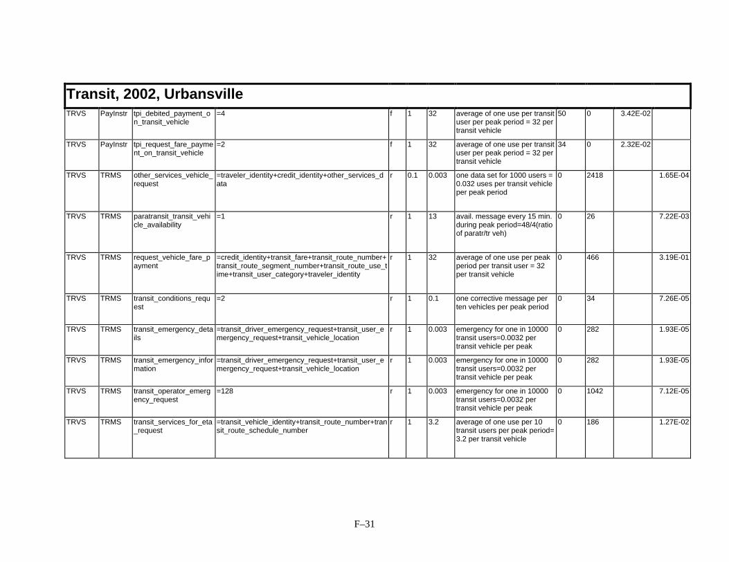
F–31
Transit, 2002, UrbansvilleTRVS PayInstr tpi_debited_payment_o
n_transit_vehicle=4 f 1 32 average of one use per transit
user per peak period = 32 pertransit vehicle
50 0 3.42E-02
TRVS PayInstr tpi_request_fare_payment_on_transit_vehicle
=2 f 1 32 average of one use per transituser per peak period = 32 pertransit vehicle
34 0 2.32E-02
TRVS TRMS other_services_vehicle_request
=traveler_identity+credit_identity+other_services_data
r 0.1 0.003 one data set for 1000 users =0.032 uses per transit vehicleper peak period
0 2418 1.65E-04
TRVS TRMS paratransit_transit_vehicle_availability
=1 r 1 13 avail. message every 15 min.during peak period=48/4(ratioof paratr/tr veh)
0 26 7.22E-03
TRVS TRMS request_vehicle_fare_payment
=credit_identity+transit_fare+transit_route_number+transit_route_segment_number+transit_route_use_time+transit_user_category+traveler_identity
r 1 32 average of one use per peakperiod per transit user = 32per transit vehicle
0 466 3.19E-01
TRVS TRMS transit_conditions_request
=2 r 1 0.1 one corrective message perten vehicles per peak period
0 34 7.26E-05
TRVS TRMS transit_emergency_details
=transit_driver_emergency_request+transit_user_emergency_request+transit_vehicle_location
r 1 0.003 emergency for one in 10000transit users=0.0032 pertransit vehicle per peak
0 282 1.93E-05
TRVS TRMS transit_emergency_information
=transit_driver_emergency_request+transit_user_emergency_request+transit_vehicle_location
r 1 0.003 emergency for one in 10000transit users=0.0032 pertransit vehicle per peak
0 282 1.93E-05
TRVS TRMS transit_operator_emergency_request
=128 r 1 0.003 emergency for one in 10000transit users=0.0032 pertransit vehicle per peak
0 1042 7.12E-05
TRVS TRMS transit_services_for_eta_request
=transit_vehicle_identity+transit_route_number+transit_route_schedule_number
r 1 3.2 average of one use per 10transit users per peak period=3.2 per transit vehicle
0 186 1.27E-02

F–32
Transit, 2002, UrbansvilleTRVS TRMS transit_user_vehicle_im
age=JPEG*(ftu_transit_user_vehicle_image) r 1 0.011 20 images per metro area per
peak period=20/1788 transitvehicles
0 73746 1.73E-02
TRVS TRMS transit_vehicle_advanced_payment_request
=advanced_charges+advanced_tolls+transit_vehicle_location
r 0.1 0.003 one data set for 1000 users =0.032 uses per transit vehicleper peak period
0 1450 9.91E-05
TRVS TRMS transit_vehicle_arrival_conditions
=128 r 1 13 updated every 60 minutesduring the peak period
0 1042 2.89E-01
TRVS TRMS transit_vehicle_collected_trip_data
=transit_vehicle_passenger_loading+transit_vehicle_running_times
r 1 13 every hour for each transitvehicle per peak period
0 1826 5.07E-01
TRVS TRMS transit_vehicle_deviations_from_schedule
=32 r 1 52 update every 15 minutesduring the peak period
0 274 3.04E-01
TRVS TRMS transit_vehicle_eta =transit_vehicle_identity+transit_vehicle_time+transit_route_number
r 1 156 updated every 5 minutesduring the peak period
0 234 7.80E-01
TRVS TRMS transit_vehicle_fare_payment_confirmation
=confirmation_flag r 1 32 average of one use per transituser per peak period = 32 pertransit vehicle
0 26 1.78E-02
TRVS TRMS transit_vehicle_location =transit_vehicle_identity+transit_vehicle_location_data
r 1 52 updated every 15 minutesduring the peak period
0 250 2.78E-01
TRVS TRMS transit_vehicle_location_for_deviation
=transit_vehicle_identity+transit_vehicle_location_data
r 1 52 updated every 15 minutesduring the peak period
0 250 2.78E-01
TRVS TRMS transit_vehicle_location_for_store
=transit_vehicle_identity+transit_vehicle_location_data
r 1 13 updated every 60 minutesduring the peak period
0 250 6.94E-02
TRVS TRMS transit_vehicle_passenger_data
=transit_passenger_numbers+transit_route_number+transit_route_segment_number+transit_route_use_time+transit_user_category+transit_vehicle_identity
r 1 52 update every 15 minutesduring the peak period
0 242 2.69E-01
TRVS TRMS transit_vehicle_schedule_deviation
=32 r 1 52 updated every 15 minutesduring the peak period
0 274 3.04E-01
TOTALS (b/s/user): 1.43E+01 3.45E+00

F–33
Emergency Management, 2002, UrbansvillePASource
PA Sink Data Flow Contents Direc.
Penetration
freq Freq. Explain Fwdbits
Revbits
Fwd rate(b/s/u)
Rev rate(b/s/u)
EM EVS emergency_vehicle_driver_outputs
=128 f 1 13 average one driver output pervehicle per hour during thepeak period
1042 0 2.89E-01
EVS EM emergency_driver_dispatch_acknowledge
=1 r 1 26 average one dispatchacknowledge per vehicle per1/2 hour during the peakperiod
0 26 1.44E-02
EVS EM emergency_driver_status_update
=16 r 1 26 average one status updateper vehicle per 1/2 hourduring the peak period
0 146 8.11E-02
EVS EM emergency_vehicle_driver_inputs
=64 r 1 13 average one driver input pervehicle per hour during thepeak period
0 530 1.47E-01
TOTALS (b/s/user): 2.89E-01 2.43E-01
Probes, 2002, UrbansvillePASource
PA Sink Data Flow Contents Direc.
Penetration
freq Freq. Explain Fwdbits
Revbits
Fwd rate(b/s/u)
Rev rate(b/s/u)
VS ISP vehicle_guidance_probe_data
=route_segment_identity+vehicle_identity r 1 12 average of 12 probe reportsper vehicle per peak period
0 314 1.74E-01
TOTALS (b/s/user): 0.00E+00 1.74E-01

F–34
Private Vehicle, 2002, ThruvillePASource
PA Sink Data Flow Contents Direc.
Penetration
freq Freq. Explain Fwdbits
Revbits
Fwd rate(b/s/u)
Rev rate(b/s/u)
EM VS emergency_request_driver_acknowledge
=1 f 0.1 1E-04 one emergency per 1000vehicles per peak period
26 0 1.20E-07
EM VS emergency_request_vehicle_acknowledge
=1 f 0.1 1E-04 one emergency per 1000vehicles per peak period
26 0 1.20E-07
LocData VS From_Location_Data_Source
=16 f 0.07 0.007 one in ten vs uses per peakperiod
146 0 4.73E-05
PayInstr VS fpi_transit_user_vehicle_input_credit_identity
=credit_identity f 1 1E-04 one in 10000 vehicles usesthis flow per peak period
178 0 8.24E-07
VS EM emergency_request_driver_details
=date+driver_personal_emergency_request+time r 0.1 1E-04 one emergency per 1000vehicles per peak period
0 282 1.31E-06
VS EM emergency_request_vehicle_details
=date+time+vehicle_emergency_request r 0.1 1E-04 one emergency per 1000vehicles per peak period
0 3354 1.55E-05
VS ISP advisory_data_request =advisory_data_scope+vehicle_location_for_advisories+transit_route_number+transit_vehicle_identity
r 0.1 0.1 one request per vehicle perpeak period
0 290 1.34E-03
VS ISP vehicle_guidance_route_accepted
=route_identity r 0.07 0.14 two acceptances per peakperiod
0 34 2.20E-04
TOTALS (b/s/user): 4.84E-05 1.58E-03

F–35
Traveler, 2002, ThruvillePASource
PA Sink Data Flow Contents Direc.
Penetration
freq Freq. Explain Fwdbits
Revbits
Fwd rate(b/s/u)
Rev rate(b/s/u)
EM PIAS emergency_request_personal_traveler_acknowledge
=confirmation_flag f 0.1 3E-05 one emergency per 2000users in peak period
26 0 3.01E-08
ISP PIAS transit_deviations_for_portables
=traveler_identity+list_size+TRANSIT_SEGS*(transit_vehicle_identity+transit_vehicle_achieved_time+transit_route_segment_number)
f 0.1 3E-04 one request per 20 pias perpeak period
3578 0 4.14E-05
ISP PIAS traveler_guidance_route =route_identity+traveler_route+traveler_identity f 0.07 0.004 one route per day per pias 18306 0 2.97E-03
LocData PIAS From_Location_Data_Source
=16 f 0.07 0.007 one in ten pias uses per peakperiod
146 0 4.73E-05
PIAS EM emergency_request_personal_traveler_details
=date+time+traveler_personal_emergency_request r 0.1 3E-05 one emergency per 2000users in peak period
0 370 4.28E-07
PIAS ISP traffic_data_portables_request
=traffic_data_request+traveler_identity r 0.1 0.05 one request per pias per peakperiod
0 250 5.79E-04
PIAS ISP transit_deviations_portables_request
=traveler_identity+transit_vehicle_deviation_request+transit_route_number
r 0.1 0.003 one request per 20 pias perpeak period
0 250 2.89E-05
TOTALS (b/s/user): 3.06E-03 6.08E-04

F–36
CVO-Local, 2002, ThruvillePASource
PA Sink Data Flow Contents Direc.
Penetration
freq Freq. Explain Fwdbits
Revbits
Fwd rate(b/s/u)
Rev rate(b/s/u)
CVS FMS cf_driver_route_instructions_request
=cv_driver_number+cv_route_number r 0.5 1 average fleet vehicle requeststwo routes per peak period
0 154 3.56E-03
CVS FMS cv_driver_route_request =trip_request+route_type r 0.5 2 average vehicle requests 4routes per peak period
0 1234 5.71E-02
CVS FMS cv_driver_storage_request
=cv_route_number r 0.5 0.05 one in ten vehicles per peakperiod
0 26 3.01E-05
CVS FMS cv_static_route_data =256 r 0.5 2 four routes per vehicle perpeak period
0 2066 9.56E-02
EM FMS cf_hazmat_request =16 f 0.1 1E-05 once per 1000 vehicles perpeak period
146 0 3.38E-08
EM VS emergency_request_driver_acknowledge
=1 f 0.1 1E-04 one emergency per 1000vehicles per peak period
26 0 6.02E-08
EM VS emergency_request_vehicle_acknowledge
=1 f 0.1 1E-04 one emergency per 1000vehicles per peak period
26 0 6.02E-08
FMS CVS cf_driver_route_instructions
=cf_driver_route+cf_driver_load_details f 0.5 1 twice per vehicle per peakperiod
5082 0 1.18E-01
FMS CVS cv_driver_route_data =cv_route_data+route_type+cv_route_number f 0.5 2 average vehicle requests fourroutes per peak period
3042 0 1.41E-01
FMS CVS cv_static_route_request =origin+destination+departure_time+desired_arrival_time+preferences+constraints
f 0.5 2 average vehicle requests fourroutes per peak period
1226 0 5.68E-02
FMS EM cf_hazmat_route_information
=cv_route_number+route r 0.1 1E-05 once per 1000 vehicles perpeak period
0 3754 8.69E-07
FMS EM cf_hazmat_vehicle_information
=28 r 0.1 1E-05 once per 1000 vehicles perpeak period
0 242 5.60E-08
FMS ImFrghtD
To_Intermodal_Freight_Depot
=64 r 0.5 0.005 one in ten of vehicles interactonce with an intermodalcarrier
0 530 6.13E-05
FMS ImFrghtS To_Intermodal_Freight_Shipper
=64 r 0.5 0.005 one in ten of vehicles interactonce with an intermodalcarrier
0 530 6.13E-05

F–37
CVO-Local, 2002, ThruvilleFMS ISP cf_route_request =trip_request+cv_route_number r 0.5 0.1 twice per vehicle per peak
period0 1234 2.86E-03
FMS ISP cv_route_request =trip_request+vehicle_identity r 0.5 0.2 four times per vehicle perpeak period
0 1354 6.27E-03
ImFrghtD FMS From_Intermodal_Freight_Depot
=64 f 0.5 0.005 one in ten of vehicles interactonce with an intermodalcarrier
530 0 6.13E-05
ImFrghtS FMS From_Intermodal_Freight_Shipper
=64 f 0.5 0.005 one in ten of vehicles interactonce with an intermodalcarrier
530 0 6.13E-05
ISP FMS cf_route =cv_route_data+cv_route_number f 0.5 0.1 twice per vehicle per peakperiod
3034 0 7.02E-03
ISP FMS cv_route =cv_route_data+vehicle_identity f 0.5 0.2 four times per vehicle perpeak period
3154 0 1.46E-02
LocData VS From_Location_Data_Source
=16 f 0.07 0.007 one in ten vehicles uses onceper peak period
146 0 2.37E-05
VS EM emergency_request_driver_details
=date+driver_personal_emergency_request+time r 0.1 1E-04 one emergency per 1000vehicles per peak period
0 282 6.53E-07
VS EM emergency_request_vehicle_details
=date+time+vehicle_emergency_request r 0.1 1E-04 one emergency per 1000vehicles per peak period
0 3354 7.76E-06
VS ISP advisory_data_request =advisory_data_scope+vehicle_location_for_advisories+transit_route_number+transit_vehicle_identity
r 0.1 0.2 two requests per vehicle perpeak period
0 290 1.34E-03
TOTALS (b/s/user): 3.37E-01 1.67E-01

F–38
CVO-Long Haul, 2002, ThruvillePASource
PA Sink Data Flow Contents Direc.
Penetration
freq Freq. Explain Fwdbits
Revbits
Fwd rate(b/s/u)
Rev rate(b/s/u)
CVAS CVCS cv_credentials_database_update
=cv_credentials_details+cv_credentials_status_code+cv_trip_classification_data
f 0.5 5E-05 one out of 1000 vehicles perpeak period
482 0 5.58E-07
CVAS CVCS cv_credentials_information_response
=cv_credentials_details+cv_credentials_status_code
f 0.5 0.005 one out of 10 vehicles 410 0 4.75E-05
CVAS CVCS cv_safety_database_update
=cv_credentials_details+cv_roadside_safety_data f 1 0.001 one out of 100 vehicles 410 0 9.49E-06
CVAS CVCS cv_safety_information_response
=cv_credentials_details+cv_roadside_safety_data f 1 0.001 one out of 100 vehicles aretransmitted
410 0 9.49E-06
CVAS FMS cf_clearance_enrollment_confirm
=confirmation_flag f 0.5 0.05 once per vehicle per peakperiod
26 0 3.01E-05
CVAS FMS cf_enrollment_information
=cv_route_number+cv_taxes_and_duties+route+route_type
f 0.5 0.025 one out of two vehiclesrequire info. per peak period
3818 0 2.21E-03
CVAS FMS cf_enrollment_payment_confirmation
=cv_route_number+cv_account_number+cv_amount_billed
f 0.5 0.05 once per vehicle per peakperiod
170 0 1.97E-04
CVAS FMS cv_enrollment_information
=cv_route_number+cv_taxes_and_duties+route+route_type
f 0.5 0.025 one out of two vehiclesrequire info. per peak period
3818 0 2.21E-03
CVAS FMS cv_enrollment_payment_confirmation
=cv_account_number+cv_amount_billed+cv_driver_credit_identity+cv_route_number
f 0.5 0.05 once per vehicle per peakperiod
346 0 4.00E-04
CVCS CVAS cv_credentials_information_request
=cv_credentials_details+cv_credentials_request_type+cv_credentials_request_identity+cv_roadside_facility_identity
r 0.5 0.005 request info on one in tenvehicles
0 554 6.41E-05
CVCS CVAS cv_roadside_daily_log =cv_roadside_facility_identity+date++cv_archived_safety_data+cv_archived_inspection_data+cv_screening_record
r 0.5 5E-04 one report per 100 vehiclesper peak period
0 3362 3.89E-05
CVCS CVAS cv_safety_information_request
=cv_credentials_details+cv_safety_information_request_identity+cv_safety_information_request_type+cv_roadside_facility_identity
r 1 0.01 request info on one in tenvehicles
0 554 1.28E-04
CVCS CVAS cv_update_safety_problems_list
=cv_credentials_details+cv_roadside_facility_identity+cv_roadside_safety_data
r 1 0.001 one out of 100 vehicles areon the list per peak period
0 538 1.25E-05

F–39
CVO-Long Haul, 2002, ThruvilleCVS FMS cf_driver_route_instructi
ons_request=cv_driver_number+cv_route_number r 0.5 0.5 average fleet vehicle requests
one route per peak period0 154 1.78E-03
CVS FMS cv_driver_enrollment_payment_request
=cv_account_number+cv_driver_credit_identity+cv_route_number
r 0.5 0.5 once per vehicle per peakperiod
0 330 3.82E-03
CVS FMS cv_driver_enrollment_request
=cv_cargo_class+cv_route_number+cv_vehicle_class+cv_weight_class
r 0.5 0.5 once per vehicle per peakperiod
0 98 1.13E-03
CVS FMS cv_driver_route_request =trip_request+route_type r 0.5 1 average vehicle requests 2routes per peak period
0 1234 2.86E-02
CVS FMS cv_driver_storage_request
=cv_route_number r 0.5 0.05 one in ten vehicles per peakperiod
0 26 3.01E-05
CVS FMS cv_static_route_data =256 r 0.5 1 two routes per vehicle perpeak period
0 2066 4.78E-02
EM FMS cf_hazmat_request =16 f 0.1 1E-05 once per 1000 vehicles perpeak period
146 0 3.38E-08
EM VS emergency_request_driver_acknowledge
=1 f 0.1 1E-04 one emergency per 1000vehicles per peak period
26 0 6.02E-08
EM VS emergency_request_vehicle_acknowledge
=1 f 0.1 1E-04 one emergency per 1000vehicles per peak period
26 0 6.02E-08
FMS CVAS cf_enroll_clearance_data
=cv_credentials_details r 0.5 0.05 once per vehicle per peakperiod
0 402 4.65E-04
FMS CVAS cf_enrollment_payment_request
=cf_manager_credit_identity+cv_account_number+cv_route_number+1.5*(cv_taxes_and_duties)
r 0.5 0.05 once per vehicle per peakperiod
0 414 4.79E-04
FMS CVAS cf_enrollment_request =cv_route_data+cv_credentials_details+cv_route_number+cv_trip_classification_data+route_type
r 0.5 0.05 once per vehicle per peakperiod
0 3498 4.05E-03
FMS CVAS cv_enrollment_payment_request
=cv_account_number+cv_driver_credit_identity+cv_route_number+1.5*(cv_taxes_and_duties)
r 0.5 0.05 once per vehicle per peakperiod
0 414 4.79E-04
FMS CVAS cv_enrollment_request =cv_route_data+cv_credentials_details+cv_trip_classification_data+cv_route_number+route_type
r 0.5 0.05 once per vehicle per peakperiod
0 3498 4.05E-03
FMS CVS cf_driver_route_instructions
=cf_driver_route+cf_driver_load_details f 0.5 0.5 once per vehicle per peakperiod
5082 0 5.88E-02

F–40
CVO-Long Haul, 2002, ThruvilleFMS CVS cv_driver_enrollment_in
formation=cv_route_number+cv_taxes_and_duties f 0.5 0.25 one out of two vehicles
require info. per peak period82 0 4.75E-04
FMS CVS cv_driver_enrollment_payment_confirmation
=cv_account_number+cv_amount_billed+cv_driver_credit_identity+cv_route_number
f 0.5 0.5 once per vehicle per peakperiod
346 0 4.00E-03
FMS CVS cv_driver_route_data =cv_route_data+route_type+cv_route_number f 0.5 1 average vehicle requests tworoutes per peak period
3042 0 7.04E-02
FMS CVS cv_static_route_request =origin+destination+departure_time+desired_arrival_time+preferences+constraints
f 0.5 1 average vehicle requests tworoutes per peak period
1226 0 2.84E-02
FMS EM cf_hazmat_route_information
=cv_route_number+route r 0.1 1E-05 once per 1000 vehicles perpeak period
0 3754 8.69E-07
FMS EM cf_hazmat_vehicle_information
=28 r 0.1 1E-05 once per 1000 vehicles perpeak period
0 242 5.60E-08
FMS ImFrghtD
To_Intermodal_Freight_Depot
=64 r 0.5 0.005 one in ten vehicles interactsonce with an intermodalcarrier
0 530 6.13E-05
FMS ImFrghtS To_Intermodal_Freight_Shipper
=64 r 0.5 0.005 one in ten vehicles interactsonce with an intermodalcarrier
0 530 6.13E-05
FMS ISP cf_route_request =trip_request+cv_route_number r 0.5 0.05 once per vehicle per peakperiod
0 1234 1.43E-03
FMS ISP cv_route_request =trip_request+vehicle_identity r 0.5 0.1 twice per vehicle per peakperiod
0 1354 3.13E-03
FMS PayInstr tpi_debited_commercial_manager_payment
=4 r 0.5 0.05 once per enrollment 0 50 5.79E-05
ImFrghtD FMS From_Intermodal_Freight_Depot
=64 f 0.5 0.005 one in ten vehicles interactsonce with an intermodalcarrier
530 0 6.13E-05
ImFrghtS FMS From_Intermodal_Freight_Shipper
=64 f 0.5 0.005 one in ten vehicles interactsonce with an intermodalcarrier
530 0 6.13E-05
ISP FMS cf_route =cv_route_data+cv_route_number f 0.5 0.05 once per vehicle per peakperiod
3034 0 3.51E-03
ISP FMS cv_route =cv_route_data+vehicle_identity f 0.5 0.1 twice per vehicle per peakperiod
3154 0 7.30E-03

F–41
CVO-Long Haul, 2002, ThruvilleLocData VS From_Location_Data_S
ource=16 f 0.07 0.007 one in ten vehicles uses once
per peak period146 0 2.37E-05
PayInstr FMS fpi_commercial_manager_input_credit_identity
=12 f 0.5 0.05 once per enrollment = onceper cv per peak period
114 0 1.32E-04
VS EM emergency_request_driver_details
=date+driver_personal_emergency_request+time r 0.1 1E-04 one emergency per 1000vehicles per peak period
0 282 6.53E-07
VS EM emergency_request_vehicle_details
=date+time+vehicle_emergency_request r 0.1 1E-04 one emergency per 1000vehicles per peak period
0 3354 7.76E-06
VS ISP advisory_data_request =advisory_data_scope+vehicle_location_for_advisories+transit_route_number+transit_vehicle_identity
r 0.1 0.2 two requests per vehicle perpeak period
0 290 1.34E-03
VS ISP vehicle_guidance_route_accepted
=route_identity r 0.07 0.14 two acceptances per peakperiod
0 34 1.10E-04
TOTALS (b/s/user): 1.78E-01 9.91E-02
Transit, 2002, ThruvillePASource
PA Sink Data Flow Contents Direc.
Penetration
freq Freq. Explain Fwdbits
Revbits
Fwd rate(b/s/u)
Rev rate(b/s/u)
PayInstr TRVS fpi_confirm_fare_payment_on_transit_vehicle
=confirmation_flag f 1 32 average of one use per transituser per peak period = 32 pertransit vehicle
26 0 1.78E-02
PayInstr TRVS fpi_transit_vehicle_tag_data
=credit_identity f 1 0.032 one data set for 1000 users =0.032 uses per transit vehicleper peak period
178 0 1.22E-04
RTS ISP traffic_data_kiosk_request
=kiosk_identity+traffic_data_request r 0.1 0.32 average of one use per transituser per peak period = 32 pertransit vehicle
0 98 6.70E-04
RTS ISP transit_deviation_kiosk_request
=kiosk_identity+transit_vehicle_deviation_request r 0.1 0.064 one in five transit users = 6.4per transit vehicle per peakperiod
0 66 9.03E-05
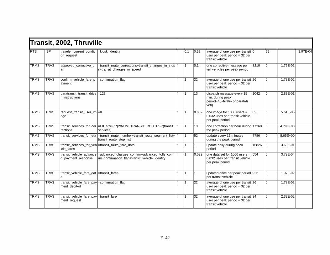
F–42
Transit, 2002, ThruvilleRTS ISP traveler_current_conditi
on_request=kiosk_identity r 0.1 0.32 average of one use per transit
user per peak period = 32 pertransit vehicle
0 58 3.97E-04
TRMS TRVS approved_corrective_plan
=transit_route_corrections+transit_changes_in_stops+transit_changes_in_speed
f 1 0.1 one corrective message perten vehicles per peak period
8210 0 1.75E-02
TRMS TRVS confirm_vehicle_fare_payment
=confirmation_flag f 1 32 average of one use per transituser per peak period = 32 pertransit vehicle
26 0 1.78E-02
TRMS TRVS paratransit_transit_driver_instructions
=128 f 1 13 dispatch message every 15min. during peakperiod=48/4(ratio of paratr/trveh)
1042 0 2.89E-01
TRMS TRVS request_transit_user_image
=8 f 1 0.032 one image for 1000 users =0.032 uses per transit vehicleper peak period
82 0 5.61E-05
TRMS TRVS transit_services_for_corrections
=list_size+1*(2/NUM_TRANSIT_ROUTES)*(transit_services)
f 1 13 one correction per hour duringthe peak period
17260 0 4.79E+00
TRMS TRVS transit_services_for_eta =transit_route_number+transit_route_segment_list+transit_route_stop_list
f 1 52 update every 15 minutesduring the peak period
7786 0 8.65E+00
TRMS TRVS transit_services_for_vehicle_fares
=transit_route_fare_data f 1 1 update daily during peakperiod
16826 0 3.60E-01
TRMS TRVS transit_vehicle_advanced_payment_response
=advanced_charges_confirm+advanced_tolls_confirm+confirmation_flag+transit_vehicle_identity
f 1 0.032 one data set for 1000 users =0.032 uses per transit vehicleper peak period
554 0 3.79E-04
TRMS TRVS transit_vehicle_fare_data
=transit_fares f 1 1 updated once per peak periodper transit vehicle
922 0 1.97E-02
TRMS TRVS transit_vehicle_fare_payment_debited
=confirmation_flag f 1 32 average of one use per transituser per peak period = 32 pertransit vehicle
26 0 1.78E-02
TRMS TRVS transit_vehicle_fare_payment_request
=transit_fare f 1 32 average of one use per transituser per peak period = 32 pertransit vehicle
34 0 2.32E-02

F–43
Transit, 2002, ThruvilleTRVS PayInstr tpi_debited_payment_o
n_transit_vehicle=4 f 1 32 average of one use per transit
user per peak period = 32 pertransit vehicle
50 0 3.42E-02
TRVS PayInstr tpi_request_fare_payment_on_transit_vehicle
=2 f 1 32 average of one use per transituser per peak period = 32 pertransit vehicle
34 0 2.32E-02
TRVS TRMS paratransit_transit_vehicle_availability
=1 r 1 13 avail. message every 15 min.during peak period=48/4(ratioof paratr/tr veh)
0 26 7.22E-03
TRVS TRMS request_vehicle_fare_payment
=credit_identity+transit_fare+transit_route_number+transit_route_segment_number+transit_route_use_time+transit_user_category+traveler_identity
r 1 32 average of one use per peakperiod per transit user = 32per transit vehicle
0 466 3.19E-01
TRVS TRMS transit_conditions_request
=2 r 1 0.1 one corrective message perten vehicles per peak period
0 34 7.26E-05
TRVS TRMS transit_services_for_eta_request
=transit_vehicle_identity+transit_route_number+transit_route_schedule_number
r 1 3.2 average of one use per 10transit users per peak period=3.2 per transit vehicle
0 186 1.27E-02
TRVS TRMS transit_user_vehicle_image
=JPEG*(ftu_transit_user_vehicle_image) r 1 0.011 20 images per metro area perpeak period=20/1788 transitvehicles
0 73746 1.73E-02
TRVS TRMS transit_vehicle_arrival_conditions
=128 r 1 13 updated every 60 minutesduring the peak period
0 1042 2.89E-01
TRVS TRMS transit_vehicle_collected_trip_data
=transit_vehicle_passenger_loading+transit_vehicle_running_times
r 1 13 every hour for each transitvehicle per peak period
0 1826 5.07E-01
TRVS TRMS transit_vehicle_deviations_from_schedule
=32 r 1 52 update every 15 minutesduring the peak period
0 274 3.04E-01
TRVS TRMS transit_vehicle_eta =transit_vehicle_identity+transit_vehicle_time+transit_route_number
r 1 156 updated every 5 minutesduring the peak period
0 234 7.80E-01
TRVS TRMS transit_vehicle_fare_payment_confirmation
=confirmation_flag r 1 32 average of one use per transituser per peak period = 32 pertransit vehicle
0 26 1.78E-02

F–44
Transit, 2002, ThruvilleTRVS TRMS transit_vehicle_location =transit_vehicle_identity+transit_vehicle_location_d
atar 1 52 updated every 15 minutes
during the peak period0 250 2.78E-01
TRVS TRMS transit_vehicle_location_for_deviation
=transit_vehicle_identity+transit_vehicle_location_data
r 1 52 updated every 15 minutesduring the peak period
0 250 2.78E-01
TRVS TRMS transit_vehicle_location_for_store
=transit_vehicle_identity+transit_vehicle_location_data
r 1 13 updated every 60 minutesduring the peak period
0 250 6.94E-02
TRVS TRMS transit_vehicle_passenger_data
=transit_passenger_numbers+transit_route_number+transit_route_segment_number+transit_route_use_time+transit_user_category+transit_vehicle_identity
r 1 52 update every 15 minutesduring the peak period
0 242 2.69E-01
TRVS TRMS transit_vehicle_schedule_deviation
=32 r 1 52 updated every 15 minutesduring the peak period
0 274 3.04E-01
TOTALS (b/s/user): 1.43E+01 3.45E+00
Emergency Management, 2002, ThruvillePASource
PA Sink Data Flow Contents Direc.
Penetration
freq Freq. Explain Fwdbits
Revbits
Fwd rate(b/s/u)
Rev rate(b/s/u)
EM EVS emergency_vehicle_driver_outputs
=128 f 1 13 average one driver output pervehicle per hour during thepeak period
1042 0 2.89E-01
EVS EM emergency_driver_dispatch_acknowledge
=1 r 1 26 average one dispatchacknowledge per vehicle per1/2 hour during the peakperiod
0 26 1.44E-02
EVS EM emergency_driver_status_update
=16 r 1 26 average one status updateper vehicle per 1/2 hourduring the peak period
0 146 8.11E-02
EVS EM emergency_vehicle_driver_inputs
=64 r 1 13 average one driver input pervehicle per hour during thepeak period
0 530 1.47E-01
TOTALS (b/s/user): 2.89E-01 2.43E-01

F–45
Probes, 2002, ThruvillePASource
PA Sink Data Flow Contents Direc.
Penetration
freq Freq. Explain Fwdbits
Revbits
Fwd rate(b/s/u)
Rev rate(b/s/u)
VS ISP vehicle_guidance_probe_data
=route_segment_identity+vehicle_identity r 1 12 average of 12 probe reportsper vehicle per peak period
0 314 1.74E-01
TOTALS (b/s/user): 0.00E+00 1.74E-01
Private Vehicle, 2002, MountainvillePASource
PA Sink Data Flow Contents Direc.
Penetration
freq Freq. Explain Fwdbits
Revbits
Fwd rate(b/s/u)
Rev rate(b/s/u)
EM VS emergency_request_driver_acknowledge
=1 f 0.1 1E-04 one emergency per 1000vehicles per peak period
26 0 1.20E-07
EM VS emergency_request_vehicle_acknowledge
=1 f 0.1 1E-04 one emergency per 1000vehicles per peak period
26 0 1.20E-07
PayInstr VS fpi_transit_user_vehicle_input_credit_identity
=credit_identity f 1 1E-04 one in 10000 vehicles usesthis flow per peak period
178 0 8.24E-07
VS EM emergency_request_driver_details
=date+driver_personal_emergency_request+time r 0.1 1E-04 one emergency per 1000vehicles per peak period
0 282 1.31E-06
VS EM emergency_request_vehicle_details
=date+time+vehicle_emergency_request r 0.1 1E-04 one emergency per 1000vehicles per peak period
0 3354 1.55E-05
TOTALS (b/s/user): 1.06E-06 1.68E-05

F–46
Traveler, 2002, MountainvillePASource
PA Sink Data Flow Contents Direc.
Penetration
freq Freq. Explain Fwdbits
Revbits
Fwd rate(b/s/u)
Rev rate(b/s/u)
EM PIAS emergency_request_personal_traveler_acknowledge
=confirmation_flag f 0.1 3E-05 one emergency per 2000users in peak period
26 0 3.01E-08
PIAS EM emergency_request_personal_traveler_details
=date+time+traveler_personal_emergency_request r 0.1 3E-05 one emergency per 2000users in peak period
0 370 4.28E-07
TOTALS (b/s/user): 3.01E-08 4.28E-07
CVO-Local, 2002, MountainvillePASource
PA Sink Data Flow Contents Direc.
Penetration
freq Freq. Explain Fwdbits
Revbits
Fwd rate(b/s/u)
Rev rate(b/s/u)
CVS FMS cf_driver_route_instructions_request
=cv_driver_number+cv_route_number r 0.5 1 average fleet vehicle requeststwo routes per peak period
0 154 3.56E-03
CVS FMS cv_driver_route_request =trip_request+route_type r 0.5 2 average vehicle requests 4routes per peak period
0 1234 5.71E-02
CVS FMS cv_driver_storage_request
=cv_route_number r 0.5 0.05 one in ten vehicles per peakperiod
0 26 3.01E-05
CVS FMS cv_static_route_data =256 r 0.5 2 four routes per vehicle perpeak period
0 2066 9.56E-02
EM FMS cf_hazmat_request =16 f 0.1 1E-05 once per 1000 vehicles perpeak period
146 0 3.38E-08
EM VS emergency_request_driver_acknowledge
=1 f 0.1 1E-04 one emergency per 1000vehicles per peak period
26 0 6.02E-08
EM VS emergency_request_vehicle_acknowledge
=1 f 0.1 1E-04 one emergency per 1000vehicles per peak period
26 0 6.02E-08
FMS CVS cf_driver_route_instructions
=cf_driver_route+cf_driver_load_details f 0.5 1 twice per vehicle per peakperiod
5082 0 1.18E-01

F–47
CVO-Local, 2002, MountainvilleFMS CVS cv_driver_route_data =cv_route_data+route_type+cv_route_number f 0.5 2 average vehicle requests four
routes per peak period3042 0 1.41E-01
FMS CVS cv_static_route_request =origin+destination+departure_time+desired_arrival_time+preferences+constraints
f 0.5 2 average vehicle requests fourroutes per peak period
1226 0 5.68E-02
FMS EM cf_hazmat_route_information
=cv_route_number+route r 0.1 1E-05 once per 1000 vehicles perpeak period
0 3754 8.69E-07
FMS EM cf_hazmat_vehicle_information
=28 r 0.1 1E-05 once per 1000 vehicles perpeak period
0 242 5.60E-08
FMS ImFrghtD
To_Intermodal_Freight_Depot
=64 r 0.5 0.005 one in ten of vehicles interactonce with an intermodalcarrier
0 530 6.13E-05
FMS ImFrghtS To_Intermodal_Freight_Shipper
=64 r 0.5 0.005 one in ten of vehicles interactonce with an intermodalcarrier
0 530 6.13E-05
FMS ISP cf_route_request =trip_request+cv_route_number r 0.5 0.1 twice per vehicle per peakperiod
0 1234 2.86E-03
FMS ISP cv_route_request =trip_request+vehicle_identity r 0.5 0.2 four times per vehicle perpeak period
0 1354 6.27E-03
ImFrghtD FMS From_Intermodal_Freight_Depot
=64 f 0.5 0.005 one in ten of vehicles interactonce with an intermodalcarrier
530 0 6.13E-05
ImFrghtS FMS From_Intermodal_Freight_Shipper
=64 f 0.5 0.005 one in ten of vehicles interactonce with an intermodalcarrier
530 0 6.13E-05
ISP FMS cf_route =cv_route_data+cv_route_number f 0.5 0.1 twice per vehicle per peakperiod
3034 0 7.02E-03
ISP FMS cv_route =cv_route_data+vehicle_identity f 0.5 0.2 four times per vehicle perpeak period
3154 0 1.46E-02
VS EM emergency_request_driver_details
=date+driver_personal_emergency_request+time r 0.1 1E-04 one emergency per 1000vehicles per peak period
0 282 6.53E-07
VS EM emergency_request_vehicle_details
=date+time+vehicle_emergency_request r 0.1 1E-04 one emergency per 1000vehicles per peak period
0 3354 7.76E-06
TOTALS (b/s/user): 3.37E-01 1.66E-01

F–48
CVO-Long Haul, 2002, MountainvillePASource
PA Sink Data Flow Contents Direc.
Penetration
freq Freq. Explain Fwdbits
Revbits
Fwd rate(b/s/u)
Rev rate(b/s/u)
CVAS CVCS cv_credentials_database_update
=cv_credentials_details+cv_credentials_status_code+cv_trip_classification_data
f 0.5 5E-05 one out of 1000 vehicles perpeak period
482 0 5.58E-07
CVAS CVCS cv_credentials_information_response
=cv_credentials_details+cv_credentials_status_code
f 0.5 0.005 one out of 10 vehicles 410 0 4.75E-05
CVAS CVCS cv_safety_database_update
=cv_credentials_details+cv_roadside_safety_data f 1 0.001 one out of 100 vehicles 410 0 9.49E-06
CVAS CVCS cv_safety_information_response
=cv_credentials_details+cv_roadside_safety_data f 1 0.001 one out of 100 vehicles aretransmitted
410 0 9.49E-06
CVAS FMS cf_clearance_enrollment_confirm
=confirmation_flag f 0.5 0.05 once per vehicle per peakperiod
26 0 3.01E-05
CVAS FMS cf_enrollment_information
=cv_route_number+cv_taxes_and_duties+route+route_type
f 0.5 0.025 one out of two vehiclesrequire info. per peak period
3818 0 2.21E-03
CVAS FMS cf_enrollment_payment_confirmation
=cv_route_number+cv_account_number+cv_amount_billed
f 0.5 0.05 once per vehicle per peakperiod
170 0 1.97E-04
CVAS FMS cv_enrollment_information
=cv_route_number+cv_taxes_and_duties+route+route_type
f 0.5 0.025 one out of two vehiclesrequire info. per peak period
3818 0 2.21E-03
CVAS FMS cv_enrollment_payment_confirmation
=cv_account_number+cv_amount_billed+cv_driver_credit_identity+cv_route_number
f 0.5 0.05 once per vehicle per peakperiod
346 0 4.00E-04
CVCS CVAS cv_credentials_information_request
=cv_credentials_details+cv_credentials_request_type+cv_credentials_request_identity+cv_roadside_facility_identity
r 0.5 0.005 request info on one in tenvehicles
0 554 6.41E-05
CVCS CVAS cv_roadside_daily_log =cv_roadside_facility_identity+date++cv_archived_safety_data+cv_archived_inspection_data+cv_screening_record
r 0.5 5E-04 one report per 100 vehiclesper peak period
0 3362 3.89E-05
CVCS CVAS cv_safety_information_request
=cv_credentials_details+cv_safety_information_request_identity+cv_safety_information_request_type+cv_roadside_facility_identity
r 1 0.01 request info on one in tenvehicles
0 554 1.28E-04
CVCS CVAS cv_update_safety_problems_list
=cv_credentials_details+cv_roadside_facility_identity+cv_roadside_safety_data
r 1 0.001 one out of 100 vehicles areon the list per peak period
0 538 1.25E-05
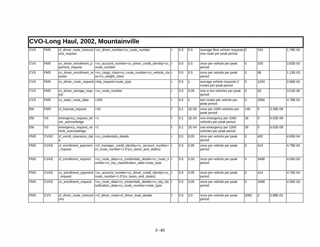
F–49
CVO-Long Haul, 2002, MountainvilleCVS FMS cf_driver_route_instructi
ons_request=cv_driver_number+cv_route_number r 0.5 0.5 average fleet vehicle requests
one route per peak period0 154 1.78E-03
CVS FMS cv_driver_enrollment_payment_request
=cv_account_number+cv_driver_credit_identity+cv_route_number
r 0.5 0.5 once per vehicle per peakperiod
0 330 3.82E-03
CVS FMS cv_driver_enrollment_request
=cv_cargo_class+cv_route_number+cv_vehicle_class+cv_weight_class
r 0.5 0.5 once per vehicle per peakperiod
0 98 1.13E-03
CVS FMS cv_driver_route_request =trip_request+route_type r 0.5 1 average vehicle requests 2routes per peak period
0 1234 2.86E-02
CVS FMS cv_driver_storage_request
=cv_route_number r 0.5 0.05 one in ten vehicles per peakperiod
0 26 3.01E-05
CVS FMS cv_static_route_data =256 r 0.5 1 two routes per vehicle perpeak period
0 2066 4.78E-02
EM FMS cf_hazmat_request =16 f 0.1 1E-05 once per 1000 vehicles perpeak period
146 0 3.38E-08
EM VS emergency_request_driver_acknowledge
=1 f 0.1 1E-04 one emergency per 1000vehicles per peak period
26 0 6.02E-08
EM VS emergency_request_vehicle_acknowledge
=1 f 0.1 1E-04 one emergency per 1000vehicles per peak period
26 0 6.02E-08
FMS CVAS cf_enroll_clearance_data
=cv_credentials_details r 0.5 0.05 once per vehicle per peakperiod
0 402 4.65E-04
FMS CVAS cf_enrollment_payment_request
=cf_manager_credit_identity+cv_account_number+cv_route_number+1.5*(cv_taxes_and_duties)
r 0.5 0.05 once per vehicle per peakperiod
0 414 4.79E-04
FMS CVAS cf_enrollment_request =cv_route_data+cv_credentials_details+cv_route_number+cv_trip_classification_data+route_type
r 0.5 0.05 once per vehicle per peakperiod
0 3498 4.05E-03
FMS CVAS cv_enrollment_payment_request
=cv_account_number+cv_driver_credit_identity+cv_route_number+1.5*(cv_taxes_and_duties)
r 0.5 0.05 once per vehicle per peakperiod
0 414 4.79E-04
FMS CVAS cv_enrollment_request =cv_route_data+cv_credentials_details+cv_trip_classification_data+cv_route_number+route_type
r 0.5 0.05 once per vehicle per peakperiod
0 3498 4.05E-03
FMS CVS cf_driver_route_instructions
=cf_driver_route+cf_driver_load_details f 0.5 0.5 once per vehicle per peakperiod
5082 0 5.88E-02

F–50
CVO-Long Haul, 2002, MountainvilleFMS CVS cv_driver_enrollment_in
formation=cv_route_number+cv_taxes_and_duties f 0.5 0.25 one out of two vehicles
require info. per peak period82 0 4.75E-04
FMS CVS cv_driver_enrollment_payment_confirmation
=cv_account_number+cv_amount_billed+cv_driver_credit_identity+cv_route_number
f 0.5 0.5 once per vehicle per peakperiod
346 0 4.00E-03
FMS CVS cv_driver_route_data =cv_route_data+route_type+cv_route_number f 0.5 1 average vehicle requests tworoutes per peak period
3042 0 7.04E-02
FMS CVS cv_static_route_request =origin+destination+departure_time+desired_arrival_time+preferences+constraints
f 0.5 1 average vehicle requests tworoutes per peak period
1226 0 2.84E-02
FMS EM cf_hazmat_route_information
=cv_route_number+route r 0.1 1E-05 once per 1000 vehicles perpeak period
0 3754 8.69E-07
FMS EM cf_hazmat_vehicle_information
=28 r 0.1 1E-05 once per 1000 vehicles perpeak period
0 242 5.60E-08
FMS ImFrghtD
To_Intermodal_Freight_Depot
=64 r 0.5 0.005 one in ten vehicles interactsonce with an intermodalcarrier
0 530 6.13E-05
FMS ImFrghtS To_Intermodal_Freight_Shipper
=64 r 0.5 0.005 one in ten vehicles interactsonce with an intermodalcarrier
0 530 6.13E-05
FMS ISP cf_route_request =trip_request+cv_route_number r 0.5 0.05 once per vehicle per peakperiod
0 1234 1.43E-03
FMS ISP cv_route_request =trip_request+vehicle_identity r 0.5 0.1 twice per vehicle per peakperiod
0 1354 3.13E-03
FMS PayInstr tpi_debited_commercial_manager_payment
=4 r 0.5 0.05 once per enrollment 0 50 5.79E-05
ImFrghtD FMS From_Intermodal_Freight_Depot
=64 f 0.5 0.005 one in ten vehicles interactsonce with an intermodalcarrier
530 0 6.13E-05
ImFrghtS FMS From_Intermodal_Freight_Shipper
=64 f 0.5 0.005 one in ten vehicles interactsonce with an intermodalcarrier
530 0 6.13E-05
ISP FMS cf_route =cv_route_data+cv_route_number f 0.5 0.05 once per vehicle per peakperiod
3034 0 3.51E-03
ISP FMS cv_route =cv_route_data+vehicle_identity f 0.5 0.1 twice per vehicle per peakperiod
3154 0 7.30E-03

F–51
CVO-Long Haul, 2002, MountainvillePayInstr FMS fpi_commercial_manag
er_input_credit_identity=12 f 0.5 0.05 once per enrollment = once
per cv per peak period114 0 1.32E-04
VS EM emergency_request_driver_details
=date+driver_personal_emergency_request+time r 0.1 1E-04 one emergency per 1000vehicles per peak period
0 282 6.53E-07
VS EM emergency_request_vehicle_details
=date+time+vehicle_emergency_request r 0.1 1E-04 one emergency per 1000vehicles per peak period
0 3354 7.76E-06
TOTALS (b/s/user): 1.78E-01 9.77E-02
Transit, 2002, MountainvillePASource
PA Sink Data Flow Contents Direc.
Penetration
freq Freq. Explain Fwdbits
Revbits
Fwd rate(b/s/u)
Rev rate(b/s/u)
PayInstr TRVS fpi_confirm_fare_payment_on_transit_vehicle
=confirmation_flag f 1 32 average of one use per transituser per peak period = 32 pertransit vehicle
26 0 1.78E-02
PayInstr TRVS fpi_transit_vehicle_tag_data
=credit_identity f 1 0.032 one data set for 1000 users =0.032 uses per transit vehicleper peak period
178 0 1.22E-04
TRMS TRVS confirm_vehicle_fare_payment
=confirmation_flag f 1 32 average of one use per transituser per peak period = 32 pertransit vehicle
26 0 1.78E-02
TRMS TRVS request_transit_user_image
=8 f 1 0.032 one image for 1000 users =0.032 uses per transit vehicleper peak period
82 0 5.61E-05
TRMS TRVS transit_services_for_vehicle_fares
=transit_route_fare_data f 1 1 update daily during peakperiod
16826 0 3.60E-01
TRMS TRVS transit_vehicle_advanced_payment_response
=advanced_charges_confirm+advanced_tolls_confirm+confirmation_flag+transit_vehicle_identity
f 1 0.032 one data set for 1000 users =0.032 uses per transit vehicleper peak period
554 0 3.79E-04

F–52
Transit, 2002, MountainvilleTRMS TRVS transit_vehicle_fare_dat
a=transit_fares f 1 1 updated once per peak period
per transit vehicle922 0 1.97E-02
TRMS TRVS transit_vehicle_fare_payment_debited
=confirmation_flag f 1 32 average of one use per transituser per peak period = 32 pertransit vehicle
26 0 1.78E-02
TRMS TRVS transit_vehicle_fare_payment_request
=transit_fare f 1 32 average of one use per transituser per peak period = 32 pertransit vehicle
34 0 2.32E-02
TRVS PayInstr tpi_debited_payment_on_transit_vehicle
=4 f 1 32 average of one use per transituser per peak period = 32 pertransit vehicle
50 0 3.42E-02
TRVS PayInstr tpi_request_fare_payment_on_transit_vehicle
=2 f 1 32 average of one use per transituser per peak period = 32 pertransit vehicle
34 0 2.32E-02
TRVS TRMS request_vehicle_fare_payment
=credit_identity+transit_fare+transit_route_number+transit_route_segment_number+transit_route_use_time+transit_user_category+traveler_identity
r 1 32 average of one use per peakperiod per transit user = 32per transit vehicle
0 466 3.19E-01
TRVS TRMS transit_user_vehicle_image
=JPEG*(ftu_transit_user_vehicle_image) r 1 0.011 20 images per metro area perpeak period=20/1788 transitvehicles
0 73746 1.73E-02
TRVS TRMS transit_vehicle_fare_payment_confirmation
=confirmation_flag r 1 32 average of one use per transituser per peak period = 32 pertransit vehicle
0 26 1.78E-02
TRVS TRMS transit_vehicle_passenger_data
=transit_passenger_numbers+transit_route_number+transit_route_segment_number+transit_route_use_time+transit_user_category+transit_vehicle_identity
r 1 52 update every 15 minutesduring the peak period
0 242 2.69E-01
TOTALS (b/s/user): 5.14E-01 6.23E-01

F–53
Emergency Management, 2002, MountainvillePASource
PA Sink Data Flow Contents Direc.
Penetration
freq Freq. Explain Fwdbits
Revbits
Fwd rate(b/s/u)
Rev rate(b/s/u)
EM EVS emergency_vehicle_driver_outputs
=128 f 1 13 average one driver output pervehicle per hour during thepeak period
1042 0 2.89E-01
EVS EM emergency_driver_dispatch_acknowledge
=1 r 1 26 average one dispatchacknowledge per vehicle per1/2 hour during the peakperiod
0 26 1.44E-02
EVS EM emergency_driver_status_update
=16 r 1 26 average one status updateper vehicle per 1/2 hourduring the peak period
0 146 8.11E-02
EVS EM emergency_vehicle_driver_inputs
=64 r 1 13 average one driver input pervehicle per hour during thepeak period
0 530 1.47E-01
TOTALS (b/s/user): 2.89E-01 2.43E-01

F–54
Private Vehicle, 2012, UrbansvillePASource
PA Sink Data Flow Contents Direc.
Penetration
freq Freq. Explain Fwdbits
Revbits
Fwd rate(b/s/u)
Rev rate(b/s/u)
EM VS emergency_request_driver_acknowledge
=1 f 0.3 3E-04 one emergency per 1000vehicles per peak period
26 0 3.61E-07
EM VS emergency_request_vehicle_acknowledge
=1 f 0.3 3E-04 one emergency per 1000vehicles per peak period
26 0 3.61E-07
ISP VS advanced_fares_and_charges_response
=confirmation_flag+credit_identity+parking_lot_cost+stored_credit+transit_fare
f 0.2 2E-04 one user per 1000 users perpeak period
234 0 2.17E-06
ISP VS advanced_tolls_and_fares_response
=confirmation_flag+credit_identity+stored_credit+toll_cost+transit_fare
f 0.2 2E-04 one user per 1000 users perpeak period
234 0 2.17E-06
ISP VS advisory_data =traffic_data_for_advisories+predicted_incidents_for_advisories+prediction_data_for_advisories+transit_services_for_advisories+transit_running_data_for_advisories
f 0.2 0.2 one set of data per peakperiod
6146 0 5.69E-02
ISP VS yellow_pages_advisory_data
=yellow_pages_data_for_advisories+yellow_pages_cost+yellow_pages_dining_reservation_confirmation+yellow_pages_lodging_reservation_confirmation+yellow_pages_ticket_purchase_confirmation
f 0.2 0.02 one yellow pages advisoryper 10 vehicles per peakperiod
10802 0 1.00E-02
LocData VS From_Location_Data_Source
=16 f 0.3 0.03 one in ten vs uses per peakperiod
146 0 2.03E-04
PayInstr VS fpi_driver_vehicle_input_credit_identity
=credit_identity f 0.2 2E-04 one vehicle per 1000 perpeak period
178 0 1.65E-06
PayInstr VS fpi_transit_user_vehicle_input_credit_identity
=credit_identity f 1 1E-04 one in 10000 vehicles usesthis flow per peak period
178 0 8.24E-07
VS EM emergency_request_driver_details
=date+driver_personal_emergency_request+time r 0.3 3E-04 one emergency per 1000vehicles per peak period
0 282 3.92E-06
VS EM emergency_request_vehicle_details
=date+time+vehicle_emergency_request r 0.3 3E-04 one emergency per 1000vehicles per peak period
0 3354 4.66E-05
VS ISP advanced_fares_and_charges_request
=0.6*(advanced_fare_details)+0.6*(advanced_parking_lot_charges)
r 0.2 2E-04 one user per 1000 users perpeak period
0 632.4 5.86E-06
VS ISP advanced_tolls_and_fares_request
=0.6*(advanced_fare_details)+0.6*(advanced_tolls) r 0.2 2E-04 one user per 1000 users perpeak period
0 642 5.94E-06

F–55
Private Vehicle, 2012, UrbansvilleVS ISP advisory_data_request =advisory_data_scope+vehicle_location_for_adviso
ries+transit_route_number+transit_vehicle_identityr 0.2 0.2 one request per vehicle per
peak period0 290 2.69E-03
VS ISP vehicle_guidance_route_accepted
=route_identity r 0.3 0.6 two acceptances per peakperiod
0 34 9.44E-04
VS ISP yellow_pages_advisory_requests
=advisory_data_scope+vehicle_location_for_advisories+transit_route_number+transit_vehicle_identity+yellow_pages_dining_reservation+yellow_pages_lodging_reservation+yellow_pages_ticket_purchase
r 0.2 0.02 one yellow pages advisoryper ten vehicles per peakperiod
0 674 6.24E-04
VS PayInstr tpi_debited_driver_payment_at_vehicle
=4 r 0.2 2E-04 one vehicle per 1000 perpeak period
0 50 4.63E-07
VS PMS advanced_parking_lot_charges_request
=credit_identity+parking_lot_identity+parking_space_details+stored_credit+vehicle_identity
r 0.2 1E-04 one user per 1000 users perpeak period
0 514 2.38E-06
VS PMS parking_lot_payment_confirmation
=confirmation_flag r 0.2 1E-04 one vehicle per 1000 perpeak period
0 26 1.20E-07
TOTALS (b/s/user): 6.71E-02 4.32E-03

F–56
Traveler, 2012, UrbansvillePASource
PA Sink Data Flow Contents Direc.
Penetration
freq Freq. Explain Fwdbits
Revbits
Fwd rate(b/s/u)
Rev rate(b/s/u)
EM PIAS emergency_request_personal_traveler_acknowledge
=confirmation_flag f 0.3 8E-05 one emergency per 2000users in peak period
26 0 9.03E-08
ISP PIAS transit_deviations_for_portables
=traveler_identity+list_size+TRANSIT_SEGS*(transit_vehicle_identity+transit_vehicle_achieved_time+transit_route_segment_number)
f 0.2 5E-04 one request per 20 pias perpeak period
3578 0 8.28E-05
ISP PIAS traveler_guidance_route =route_identity+traveler_route+traveler_identity f 0.3 0.015 one route per day per pias 18306 0 1.27E-02
ISP PIAS traveler_personal_payment_confirmation
=advanced_tolls_confirm+advanced_fares_confirm+advanced_parking_lot_charges_confirm+credit_identity+stored_credit+traveler_identity+traveler_total_trip_cost
f 0.2 0.01 one payment per 10 pias perpeak period
818 0 3.79E-04
ISP PIAS traveler_personal_transaction_confirmation
=credit_identity+traveler_identity+transaction_number+yellow_pages_cost+yellow_pages_lodging_reservation_confirmation+yellow_pages_dining_reservation_confirmation+yellow_pages_ticket_purchase_confirmation
f 0.2 0.01 one confirmation per 10 piasper day
650 0 3.01E-04
ISP PIAS traveler_personal_yellow_pages_data
=traveler_identity+0.01*(yellow_pages_general_information+yellow_pages_specific_information+yellow_pages_transaction_information)
f 0.2 0.1 one yellow pages responseper pias per peak period
1140 0 5.28E-03
LocData PIAS From_Location_Data_Source
=16 f 0.3 0.03 one in ten pias uses per peakperiod
146 0 2.03E-04
PayInstr PIAS fpi_traveler_personal_input_credit_identity
=credit_identity f 0.2 0.01 one transaction per 10 piasper day
178 0 8.24E-05
PIAS EM emergency_request_personal_traveler_details
=date+time+traveler_personal_emergency_request r 0.3 8E-05 one emergency per 2000users in peak period
0 370 1.28E-06
PIAS ISP traffic_data_portables_request
=traffic_data_request+traveler_identity r 0.2 0.1 one request per pias per peakperiod
0 250 1.16E-03
PIAS ISP transit_deviations_portables_request
=traveler_identity+transit_vehicle_deviation_request+transit_route_number
r 0.2 0.005 one request per 20 pias perpeak period
0 250 5.79E-05

F–57
Traveler, 2012, UrbansvillePIAS ISP traveler_personal_curre
nt_condition_request=traveler_identity r 0.2 0.1 one request per pias per peak
period0 210 9.72E-04
PIAS ISP traveler_personal_payment_information
=credit_identity+parking_space_details+ride_segments+stored_credit+toll_segments+traveler_identity
r 0.2 0.01 one payment per 10 pias perpeak period
0 1130 5.23E-04
PIAS ISP traveler_personal_transaction_request
=yellow_pages_dining_reservation+yellow_pages_lodging_reservation+yellow_pages_ticket_purchase
r 0.2 0.01 one request per 10 pias perpeak period
0 402 1.86E-04
PIAS ISP traveler_personal_yellow_pages_information_request
=1 r 0.2 0.1 one yellow pages request perpias per peak period
0 26 1.20E-04
PIAS PayInstr tpi_debited_payment_at_personal_device
=4 r 0.2 0.01 one transaction per 10 piasper day
0 50 2.31E-05
PIAS TRMS transit_services_portables_request
=destination+origin+traveler_identity r 0.2 0.01 one request per 10 pias perpeak period
0 466 2.16E-04
TRMS PIAS transit_services_for_portables
=traveler_identity+2*(transit_services_for_output) f 0.2 0.003 one request per 20 pias perpeak period
2530 0 3.87E-04
TOTALS (b/s/user): 1.94E-02 3.26E-03

F–58
CVO-Local, 2012, UrbansvillePASource
PA Sink Data Flow Contents Direc.
Penetration
freq Freq. Explain Fwdbits
Revbits
Fwd rate(b/s/u)
Rev rate(b/s/u)
CVS FMS cf_driver_route_instructions_request
=cv_driver_number+cv_route_number r 0.8 1.6 average fleet vehicle requeststwo routes per peak period
0 154 5.70E-03
CVS FMS cv_driver_route_request =trip_request+route_type r 0.8 3.2 average vehicle requests 4routes per peak period
0 1234 9.14E-02
CVS FMS cv_driver_storage_request
=cv_route_number r 0.8 0.08 one in ten vehicles per peakperiod
0 26 4.81E-05
CVS FMS cv_static_route_data =256 r 0.8 3.2 four routes per vehicle perpeak period
0 2066 1.53E-01
EM FMS cf_hazmat_request =16 f 0.5 5E-05 once per 1000 vehicles perpeak period
146 0 1.69E-07
EM VS emergency_request_driver_acknowledge
=1 f 0.3 3E-04 one emergency per 1000vehicles per peak period
26 0 1.81E-07
EM VS emergency_request_vehicle_acknowledge
=1 f 0.3 3E-04 one emergency per 1000vehicles per peak period
26 0 1.81E-07
FMS CVS cf_driver_route_instructions
=cf_driver_route+cf_driver_load_details f 0.8 1.6 twice per vehicle per peakperiod
5082 0 1.88E-01
FMS CVS cv_driver_route_data =cv_route_data+route_type+cv_route_number f 0.8 3.2 average vehicle requests fourroutes per peak period
3042 0 2.25E-01
FMS CVS cv_static_route_request =origin+destination+departure_time+desired_arrival_time+preferences+constraints
f 0.8 3.2 average vehicle requests fourroutes per peak period
1226 0 9.08E-02
FMS EM cf_hazmat_route_information
=cv_route_number+route r 0.5 5E-05 once per 1000 vehicles perpeak period
0 3754 4.34E-06
FMS EM cf_hazmat_vehicle_information
=28 r 0.5 5E-05 once per 1000 vehicles perpeak period
0 242 2.80E-07
FMS ImFrghtD
To_Intermodal_Freight_Depot
=64 r 0.8 0.008 one in ten of vehicles interactonce with an intermodalcarrier
0 530 9.81E-05
FMS ImFrghtS To_Intermodal_Freight_Shipper
=64 r 0.8 0.008 one in ten of vehicles interactonce with an intermodalcarrier
0 530 9.81E-05

F–59
CVO-Local, 2012, UrbansvilleFMS ISP cf_route_request =trip_request+cv_route_number r 0.8 0.16 twice per vehicle per peak
period0 1234 4.57E-03
FMS ISP cv_route_request =trip_request+vehicle_identity r 0.8 0.32 four times per vehicle perpeak period
0 1354 1.00E-02
ImFrghtD FMS From_Intermodal_Freight_Depot
=64 f 0.8 0.008 one in ten of vehicles interactonce with an intermodalcarrier
530 0 9.81E-05
ImFrghtS FMS From_Intermodal_Freight_Shipper
=64 f 0.8 0.008 one in ten of vehicles interactonce with an intermodalcarrier
530 0 9.81E-05
ISP FMS cf_route =cv_route_data+cv_route_number f 0.8 0.16 twice per vehicle per peakperiod
3034 0 1.12E-02
ISP FMS cv_route =cv_route_data+vehicle_identity f 0.8 0.32 four times per vehicle perpeak period
3154 0 2.34E-02
ISP VS advanced_fares_and_charges_response
=confirmation_flag+credit_identity+parking_lot_cost+stored_credit+transit_fare
f 0.2 2E-04 one user per 1000 users perpeak period
234 0 1.08E-06
ISP VS advanced_tolls_and_fares_response
=confirmation_flag+credit_identity+stored_credit+toll_cost+transit_fare
f 0.2 2E-04 one user per 1000 users perpeak period
234 0 1.08E-06
ISP VS advisory_data =traffic_data_for_advisories+predicted_incidents_for_advisories+prediction_data_for_advisories+transit_services_for_advisories+transit_running_data_for_advisories
f 0.2 0.4 two sets of data per peakperiod
6146 0 5.69E-02
ISP VS yellow_pages_advisory_data
=yellow_pages_data_for_advisories+yellow_pages_cost+yellow_pages_dining_reservation_confirmation+yellow_pages_lodging_reservation_confirmation+yellow_pages_ticket_purchase_confirmation
f 0.2 0.02 one yellow pages advisoryper 10 vehicles per peakperiod
10802 0 5.00E-03
LocData VS From_Location_Data_Source
=16 f 0.3 0.03 one in ten vehicles uses onceper peak period
146 0 1.01E-04
PayInstr VS fpi_driver_vehicle_input_credit_identity
=credit_identity f 0.2 2E-04 one vehicle per 1000 perpeak period
178 0 8.24E-07
VS EM emergency_request_driver_details
=date+driver_personal_emergency_request+time r 0.3 3E-04 one emergency per 1000vehicles per peak period
0 282 1.96E-06
VS EM emergency_request_vehicle_details
=date+time+vehicle_emergency_request r 0.3 3E-04 one emergency per 1000vehicles per peak period
0 3354 2.33E-05

F–60
CVO-Local, 2012, UrbansvilleVS ISP advanced_fares_and_c
harges_request=0.6*(advanced_fare_details)+0.6*(advanced_parking_lot_charges)
r 0.2 2E-04 one user per 1000 users perpeak period
0 632.4 2.93E-06
VS ISP advanced_tolls_and_fares_request
=0.6*(advanced_fare_details)+0.6*(advanced_tolls) r 0.2 2E-04 one user per 1000 users perpeak period
0 642 2.97E-06
VS ISP advisory_data_request =advisory_data_scope+vehicle_location_for_advisories+transit_route_number+transit_vehicle_identity
r 0.2 0.4 two requests per vehicle perpeak period
0 290 2.69E-03
VS ISP yellow_pages_advisory_requests
=advisory_data_scope+vehicle_location_for_advisories+transit_route_number+transit_vehicle_identity+yellow_pages_dining_reservation+yellow_pages_lodging_reservation+yellow_pages_ticket_purchase
r 0.2 0.02 one yellow pages advisoryper 10 vehicles per peakperiod
0 674 3.12E-04
VS PayInstr tpi_debited_driver_payment_at_vehicle
=4 r 0.2 2E-04 one vehicle per 1000 perpeak period
0 50 2.31E-07
VS PMS advanced_parking_lot_charges_request
=credit_identity+parking_lot_identity+parking_space_details+stored_credit+vehicle_identity
r 0.2 1E-04 one user per 1000 users perpeak period
0 514 1.19E-06
VS PMS parking_lot_payment_confirmation
=confirmation_flag r 0.2 1E-04 one vehicle per 1000 perpeak period
0 26 6.02E-08
TOTALS (b/s/user): 6.01E-01 2.68E-01

F–61
CVO-Long Haul, 2012, UrbansvillePASource
PA Sink Data Flow Contents Direc.
Penetration
freq Freq. Explain Fwdbits
Revbits
Fwd rate(b/s/u)
Rev rate(b/s/u)
CVAS CVCS cv_credentials_database_update
=cv_credentials_details+cv_credentials_status_code+cv_trip_classification_data
f 0.85 9E-05 one out of 1000 vehicles perpeak period
482 0 9.48E-07
CVAS CVCS cv_credentials_information_response
=cv_credentials_details+cv_credentials_status_code
f 0.85 0.009 one out of 10 vehicles 410 0 8.07E-05
CVAS CVCS cv_safety_database_update
=cv_credentials_details+cv_roadside_safety_data f 1 0.001 one out of 100 vehicles 410 0 9.49E-06
CVAS CVCS cv_safety_information_response
=cv_credentials_details+cv_roadside_safety_data f 1 0.001 one out of 100 vehicles aretransmitted
410 0 9.49E-06
CVAS FMS cf_clearance_enrollment_confirm
=confirmation_flag f 0.85 0.085 once per vehicle per peakperiod
26 0 5.12E-05
CVAS FMS cf_enrollment_information
=cv_route_number+cv_taxes_and_duties+route+route_type
f 0.85 0.043 one out of two vehiclesrequire info. per peak period
3818 0 3.76E-03
CVAS FMS cf_enrollment_payment_confirmation
=cv_route_number+cv_account_number+cv_amount_billed
f 0.85 0.085 once per vehicle per peakperiod
170 0 3.34E-04
CVAS FMS cv_enrollment_information
=cv_route_number+cv_taxes_and_duties+route+route_type
f 0.85 0.043 one out of two vehiclesrequire info. per peak period
3818 0 3.76E-03
CVAS FMS cv_enrollment_payment_confirmation
=cv_account_number+cv_amount_billed+cv_driver_credit_identity+cv_route_number
f 0.85 0.085 once per vehicle per peakperiod
346 0 6.81E-04
CVCS CVAS cv_credentials_information_request
=cv_credentials_details+cv_credentials_request_type+cv_credentials_request_identity+cv_roadside_facility_identity
r 0.85 0.009 request info on one in tenvehicles
0 554 1.09E-04
CVCS CVAS cv_roadside_daily_log =cv_roadside_facility_identity+date++cv_archived_safety_data+cv_archived_inspection_data+cv_screening_record
r 0.85 9E-04 one report per 100 vehiclesper peak period
0 3362 6.62E-05
CVCS CVAS cv_safety_information_request
=cv_credentials_details+cv_safety_information_request_identity+cv_safety_information_request_type+cv_roadside_facility_identity
r 1 0.01 request info on one in tenvehicles
0 554 1.28E-04
CVCS CVAS cv_update_safety_problems_list
=cv_credentials_details+cv_roadside_facility_identity+cv_roadside_safety_data
r 1 0.001 one out of 100 vehicles areon the list per peak period
0 538 1.25E-05

F–62
CVO-Long Haul, 2012, UrbansvilleCVS FMS cf_driver_route_instructi
ons_request=cv_driver_number+cv_route_number r 0.8 0.8 average fleet vehicle requests
one route per peak period0 154 2.85E-03
CVS FMS cv_driver_enrollment_payment_request
=cv_account_number+cv_driver_credit_identity+cv_route_number
r 0.85 0.85 once per vehicle per peakperiod
0 330 6.49E-03
CVS FMS cv_driver_enrollment_request
=cv_cargo_class+cv_route_number+cv_vehicle_class+cv_weight_class
r 0.85 0.85 once per vehicle per peakperiod
0 98 1.93E-03
CVS FMS cv_driver_route_request =trip_request+route_type r 0.8 1.6 average vehicle requests 2routes per peak period
0 1234 4.57E-02
CVS FMS cv_driver_storage_request
=cv_route_number r 0.8 0.08 one in ten vehicles per peakperiod
0 26 4.81E-05
CVS FMS cv_static_route_data =256 r 0.8 1.6 two routes per vehicle perpeak period
0 2066 7.65E-02
EM FMS cf_hazmat_request =16 f 0.5 5E-05 once per 1000 vehicles perpeak period
146 0 1.69E-07
EM VS emergency_request_driver_acknowledge
=1 f 0.3 3E-04 one emergency per 1000vehicles per peak period
26 0 1.81E-07
EM VS emergency_request_vehicle_acknowledge
=1 f 0.3 3E-04 one emergency per 1000vehicles per peak period
26 0 1.81E-07
FMS CVAS cf_enroll_clearance_data
=cv_credentials_details r 0.85 0.085 once per vehicle per peakperiod
0 402 7.91E-04
FMS CVAS cf_enrollment_payment_request
=cf_manager_credit_identity+cv_account_number+cv_route_number+1.5*(cv_taxes_and_duties)
r 0.85 0.085 once per vehicle per peakperiod
0 414 8.15E-04
FMS CVAS cf_enrollment_request =cv_route_data+cv_credentials_details+cv_route_number+cv_trip_classification_data+route_type
r 0.85 0.085 once per vehicle per peakperiod
0 3498 6.88E-03
FMS CVAS cv_enrollment_payment_request
=cv_account_number+cv_driver_credit_identity+cv_route_number+1.5*(cv_taxes_and_duties)
r 0.85 0.085 once per vehicle per peakperiod
0 414 8.15E-04
FMS CVAS cv_enrollment_request =cv_route_data+cv_credentials_details+cv_trip_classification_data+cv_route_number+route_type
r 0.85 0.085 once per vehicle per peakperiod
0 3498 6.88E-03
FMS CVS cf_driver_route_instructions
=cf_driver_route+cf_driver_load_details f 0.8 0.8 once per vehicle per peakperiod
5082 0 9.41E-02

F–63
CVO-Long Haul, 2012, UrbansvilleFMS CVS cv_driver_enrollment_in
formation=cv_route_number+cv_taxes_and_duties f 0.85 0.425 one out of two vehicles
require info. per peak period82 0 8.07E-04
FMS CVS cv_driver_enrollment_payment_confirmation
=cv_account_number+cv_amount_billed+cv_driver_credit_identity+cv_route_number
f 0.85 0.85 once per vehicle per peakperiod
346 0 6.81E-03
FMS CVS cv_driver_route_data =cv_route_data+route_type+cv_route_number f 0.8 1.6 average vehicle requests tworoutes per peak period
3042 0 1.13E-01
FMS CVS cv_static_route_request =origin+destination+departure_time+desired_arrival_time+preferences+constraints
f 0.8 1.6 average vehicle requests tworoutes per peak period
1226 0 4.54E-02
FMS EM cf_hazmat_route_information
=cv_route_number+route r 0.5 5E-05 once per 1000 vehicles perpeak period
0 3754 4.34E-06
FMS EM cf_hazmat_vehicle_information
=28 r 0.5 5E-05 once per 1000 vehicles perpeak period
0 242 2.80E-07
FMS ImFrghtD
To_Intermodal_Freight_Depot
=64 r 0.8 0.008 one in ten vehicles interactsonce with an intermodalcarrier
0 530 9.81E-05
FMS ImFrghtS To_Intermodal_Freight_Shipper
=64 r 0.8 0.008 one in ten vehicles interactsonce with an intermodalcarrier
0 530 9.81E-05
FMS ISP cf_route_request =trip_request+cv_route_number r 0.8 0.08 once per vehicle per peakperiod
0 1234 2.29E-03
FMS ISP cv_route_request =trip_request+vehicle_identity r 0.8 0.16 twice per vehicle per peakperiod
0 1354 5.01E-03
FMS PayInstr tpi_debited_commercial_manager_payment
=4 r 0.85 0.085 once per enrollment 0 50 9.84E-05
ImFrghtD FMS From_Intermodal_Freight_Depot
=64 f 0.8 0.008 one in ten vehicles interactsonce with an intermodalcarrier
530 0 9.81E-05
ImFrghtS FMS From_Intermodal_Freight_Shipper
=64 f 0.8 0.008 one in ten vehicles interactsonce with an intermodalcarrier
530 0 9.81E-05
ISP FMS cf_route =cv_route_data+cv_route_number f 0.8 0.08 once per vehicle per peakperiod
3034 0 5.62E-03
ISP FMS cv_route =cv_route_data+vehicle_identity f 0.8 0.16 twice per vehicle per peakperiod
3154 0 1.17E-02

F–64
CVO-Long Haul, 2012, UrbansvilleISP VS advanced_fares_and_c
harges_response=confirmation_flag+credit_identity+parking_lot_cost+stored_credit+transit_fare
f 0.2 2E-04 one user per 1000 users perpeak period
234 0 1.08E-06
ISP VS advanced_tolls_and_fares_response
=confirmation_flag+credit_identity+stored_credit+toll_cost+transit_fare
f 0.2 2E-04 one user per 1000 users perpeak period
234 0 1.08E-06
ISP VS advisory_data =traffic_data_for_advisories+predicted_incidents_for_advisories+prediction_data_for_advisories+transit_services_for_advisories+transit_running_data_for_advisories
f 0.2 0.2 one set of data per peakperiod
6146 0 2.85E-02
ISP VS yellow_pages_advisory_data
=yellow_pages_data_for_advisories+yellow_pages_cost+yellow_pages_dining_reservation_confirmation+yellow_pages_lodging_reservation_confirmation+yellow_pages_ticket_purchase_confirmation
f 0.2 0.02 one yellow pages advisoryper 10 vehicles per peakperiod
10802 0 5.00E-03
LocData VS From_Location_Data_Source
=16 f 0.3 0.03 one in ten vehicles uses onceper peak period
146 0 1.01E-04
PayInstr FMS fpi_commercial_manager_input_credit_identity
=12 f 0.85 0.085 once per enrollment = onceper cv per peak period
114 0 2.24E-04
PayInstr VS fpi_driver_vehicle_input_credit_identity
=credit_identity f 0.2 2E-04 one vehicle per 1000 perpeak period
178 0 8.24E-07
VS EM emergency_request_driver_details
=date+driver_personal_emergency_request+time r 0.3 3E-04 one emergency per 1000vehicles per peak period
0 282 1.96E-06
VS EM emergency_request_vehicle_details
=date+time+vehicle_emergency_request r 0.3 3E-04 one emergency per 1000vehicles per peak period
0 3354 2.33E-05
VS ISP advanced_fares_and_charges_request
=0.6*(advanced_fare_details)+0.6*(advanced_parking_lot_charges)
r 0.2 2E-04 one user per 1000 users perpeak period
0 632.4 2.93E-06
VS ISP advanced_tolls_and_fares_request
=0.6*(advanced_fare_details)+0.6*(advanced_tolls) r 0.2 2E-04 one user per 1000 users perpeak period
0 642 2.97E-06
VS ISP advisory_data_request =advisory_data_scope+vehicle_location_for_advisories+transit_route_number+transit_vehicle_identity
r 0.2 0.4 two requests per vehicle perpeak period
0 290 2.69E-03
VS ISP vehicle_guidance_route_accepted
=route_identity r 0.3 0.6 two acceptances per peakperiod
0 34 4.72E-04

F–65
CVO-Long Haul, 2012, UrbansvilleVS ISP yellow_pages_advisory_
requests=advisory_data_scope+vehicle_location_for_advisories+transit_route_number+transit_vehicle_identity+yellow_pages_dining_reservation+yellow_pages_lodging_reservation+yellow_pages_ticket_purchase
r 0.2 0.02 one yellow pages advisoryper 10 vehicles per peakperiod
0 674 3.12E-04
VS PayInstr tpi_debited_driver_payment_at_vehicle
=4 r 0.2 2E-04 one vehicle per 1000 perpeak period
0 50 2.31E-07
VS PMS advanced_parking_lot_charges_request
=credit_identity+parking_lot_identity+parking_space_details+stored_credit+vehicle_identity
r 0.2 1E-04 one user per 1000 users perpeak period
0 514 1.19E-06
VS PMS parking_lot_payment_confirmation
=confirmation_flag r 0.2 1E-04 one vehicle per 1000 perpeak period
0 26 6.02E-08
TOTALS (b/s/user): 3.20E-01 1.61E-01
Transit, 2012, UrbansvillePASource
PA Sink Data Flow Contents Direc.
Penetration
freq Freq. Explain Fwdbits
Revbits
Fwd rate(b/s/u)
Rev rate(b/s/u)
ISP RTS advanced_tolls_and_charges_roadside_confirm
=advanced_charges_confirm+advanced_tolls_confirm+confirmation_flag
f 0.2 6E-04 one use per 1000 transitusers per peak period, or0.032/transit vehicle
426 0 5.83E-06
ISP RTS traveler_payment_confirmation
=advanced_tolls_confirm+advanced_fares_confirm+advanced_parking_lot_charges_confirm+credit_identity+kiosk_identity+stored_credit+traveler_total_trip_cost
f 0.2 6E-04 one use per 1000 transitusers per peak period, or0.032/transit vehicle
666 0 9.11E-06
ISP RTS traveler_transaction_confirmation
=credit_identity+kiosk_identity+transaction_number+yellow_pages_cost+yellow_pages_lodging_reservation_confirmation+yellow_pages_dining_reservation_confirmation+yellow_pages_ticket_purchase_confirmation
f 0.2 6E-04 one use per 1000 transitusers per peak period, or0.032/transit vehicle
498 0 6.81E-06
ISP RTS traveler_yellow_pages_data
=kiosk_identity+0.01*(yellow_pages_general_information+yellow_pages_specific_information+yellow_pages_transaction_information)
f 0.2 6E-04 one use per 1000 transitusers per peak period, or0.032/transit vehicle
987.7 0 1.35E-05

F–66
Transit, 2012, UrbansvillePayInstr RTS fpi_confirm_fare_payme
nt_at_roadside=confirmation_flag f 0.2 0.128 one in five transit users = 6.4
per transit vehicle per peakperiod
26 0 7.11E-05
PayInstr RTS fpi_transit_roadside_tag_data
=credit_identity f 0.2 6E-04 one data set for 1000 users =0.032 uses per transit vehicleper peak period
178 0 2.43E-06
PayInstr RTS fpi_transit_user_roadside_input_credit_identity
=credit_identity f 0.2 6E-04 one data set for 1000 users =0.032 uses per transit vehicleper peak period
178 0 2.43E-06
PayInstr RTS fpi_traveler_roadside_input_credit_identity
=credit_identity f 0.2 6E-04 one data set for 1000 users =0.032 uses per transit vehicleper peak period
178 0 2.43E-06
PayInstr TRVS fpi_confirm_fare_payment_on_transit_vehicle
=confirmation_flag f 1 32 average of one use per transituser per peak period = 32 pertransit vehicle
26 0 1.78E-02
PayInstr TRVS fpi_transit_vehicle_tag_data
=credit_identity f 1 0.032 one data set for 1000 users =0.032 uses per transit vehicleper peak period
178 0 1.22E-04
RTS EM emergency_request_kiosk_traveler_details
=date+time+traveler_personal_emergency_request r 1 0.003 one emergency per 1000transit users per peak period,or 0.032/transit vehicle
0 370 2.53E-05
RTS ISP advanced_tolls_and_charges_roadside_request
=0.6*(advanced_charges)+0.6*(advanced_tolls) r 0.2 6E-04 one use per 1000 transitusers per peak period, or0.032/transit vehicle
0 738 1.01E-05
RTS ISP traffic_data_kiosk_request
=kiosk_identity+traffic_data_request r 0.2 0.64 average of one use per transituser per peak period = 32 pertransit vehicle
0 98 1.34E-03
RTS ISP transit_deviation_kiosk_request
=kiosk_identity+transit_vehicle_deviation_request r 0.2 0.128 one in five transit users = 6.4per transit vehicle per peakperiod
0 66 1.81E-04

F–67
Transit, 2012, UrbansvilleRTS ISP traveler_current_conditi
on_request=kiosk_identity r 0.2 0.64 average of one use per transit
user per peak period = 32 pertransit vehicle
0 58 7.93E-04
RTS ISP traveler_payment_information
=credit_identity+kiosk_identity+parking_space_details+ride_segments+stored_credit+toll_segments
r 0.2 6E-04 one use per 1000 transitusers per peak period, or0.032/transit vehicle
0 978 1.34E-05
RTS ISP traveler_transaction_request
=yellow_pages_dining_reservation+yellow_pages_lodging_reservation+yellow_pages_ticket_purchase
r 0.2 6E-04 one use per 1000 transitusers per peak period, or0.032/transit vehicle
0 402 5.50E-06
RTS ISP traveler_trip_confirmation
=paratransit_service_confirmation+traveler_identity+traveler_rideshare_confirmation
r 0.2 6E-04 one use per 1000 transitusers per peak period, or0.032/transit vehicle
0 858 1.17E-05
RTS ISP traveler_trip_request =trip_request+traveler_identity+traveler_rideshare_request
r 0.2 6E-04 one use per 1000 transitusers per peak period, or0.032/transit vehicle
0 1434 1.96E-05
RTS ISP traveler_yellow_pages_information_request
=1 r 0.2 6E-04 one use per 1000 transitusers per peak period, or0.032/transit vehicle
0 26 3.56E-07
RTS PayInstr tpi_debited_fare_payment_at_roadside
=4 r 0.2 0.128 one in five transit users = 6.4per transit vehicle per peakperiod
0 50 1.37E-04
RTS PayInstr tpi_debited_transit_user_payment_at_roadside
=4 r 0.2 0.064 one in ten transit users = 3.2per transit vehicle per peakperiod
0 50 6.84E-05
RTS PayInstr tpi_debited_traveler_payment_at_roadside
=4 r 0.2 6E-04 one data set for 1000 users =0.032 uses per transit vehicleper peak period
0 50 6.84E-07
RTS PayInstr tpi_request_fare_payment_at_roadside
=2 r 0.2 6E-04 one data set for 1000 users =0.032 uses per transit vehicleper peak period
0 34 4.65E-07
TRMS TRVS approved_corrective_plan
=transit_route_corrections+transit_changes_in_stops+transit_changes_in_speed
f 1 0.1 one corrective message perten vehicles per peak period
8210 0 1.75E-02
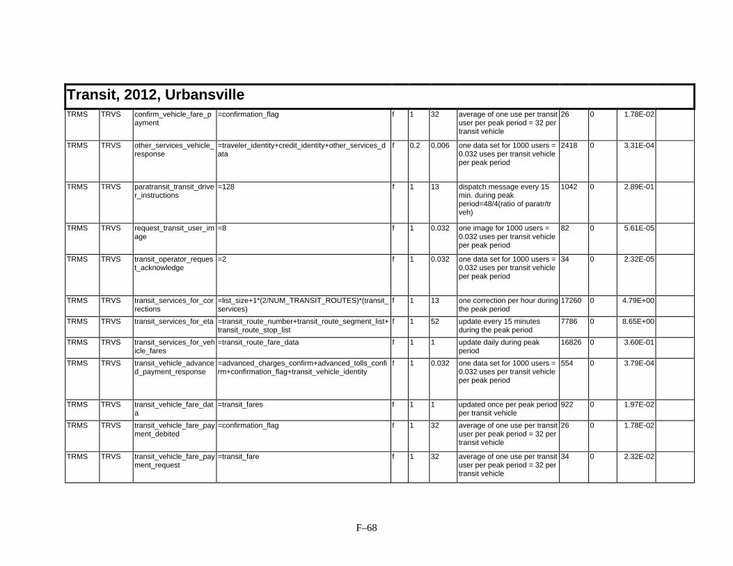
F–68
Transit, 2012, UrbansvilleTRMS TRVS confirm_vehicle_fare_p
ayment=confirmation_flag f 1 32 average of one use per transit
user per peak period = 32 pertransit vehicle
26 0 1.78E-02
TRMS TRVS other_services_vehicle_response
=traveler_identity+credit_identity+other_services_data
f 0.2 0.006 one data set for 1000 users =0.032 uses per transit vehicleper peak period
2418 0 3.31E-04
TRMS TRVS paratransit_transit_driver_instructions
=128 f 1 13 dispatch message every 15min. during peakperiod=48/4(ratio of paratr/trveh)
1042 0 2.89E-01
TRMS TRVS request_transit_user_image
=8 f 1 0.032 one image for 1000 users =0.032 uses per transit vehicleper peak period
82 0 5.61E-05
TRMS TRVS transit_operator_request_acknowledge
=2 f 1 0.032 one data set for 1000 users =0.032 uses per transit vehicleper peak period
34 0 2.32E-05
TRMS TRVS transit_services_for_corrections
=list_size+1*(2/NUM_TRANSIT_ROUTES)*(transit_services)
f 1 13 one correction per hour duringthe peak period
17260 0 4.79E+00
TRMS TRVS transit_services_for_eta =transit_route_number+transit_route_segment_list+transit_route_stop_list
f 1 52 update every 15 minutesduring the peak period
7786 0 8.65E+00
TRMS TRVS transit_services_for_vehicle_fares
=transit_route_fare_data f 1 1 update daily during peakperiod
16826 0 3.60E-01
TRMS TRVS transit_vehicle_advanced_payment_response
=advanced_charges_confirm+advanced_tolls_confirm+confirmation_flag+transit_vehicle_identity
f 1 0.032 one data set for 1000 users =0.032 uses per transit vehicleper peak period
554 0 3.79E-04
TRMS TRVS transit_vehicle_fare_data
=transit_fares f 1 1 updated once per peak periodper transit vehicle
922 0 1.97E-02
TRMS TRVS transit_vehicle_fare_payment_debited
=confirmation_flag f 1 32 average of one use per transituser per peak period = 32 pertransit vehicle
26 0 1.78E-02
TRMS TRVS transit_vehicle_fare_payment_request
=transit_fare f 1 32 average of one use per transituser per peak period = 32 pertransit vehicle
34 0 2.32E-02

F–69
Transit, 2012, UrbansvilleTRVS PayInstr tpi_debited_payment_o
n_transit_vehicle=4 f 1 32 average of one use per transit
user per peak period = 32 pertransit vehicle
50 0 3.42E-02
TRVS PayInstr tpi_request_fare_payment_on_transit_vehicle
=2 f 1 32 average of one use per transituser per peak period = 32 pertransit vehicle
34 0 2.32E-02
TRVS TRMS other_services_vehicle_request
=traveler_identity+credit_identity+other_services_data
r 0.2 0.006 one data set for 1000 users =0.032 uses per transit vehicleper peak period
0 2418 3.31E-04
TRVS TRMS paratransit_transit_vehicle_availability
=1 r 1 13 avail. message every 15 min.during peak period=48/4(ratioof paratr/tr veh)
0 26 7.22E-03
TRVS TRMS request_vehicle_fare_payment
=credit_identity+transit_fare+transit_route_number+transit_route_segment_number+transit_route_use_time+transit_user_category+traveler_identity
r 1 32 average of one use per peakperiod per transit user = 32per transit vehicle
0 466 3.19E-01
TRVS TRMS transit_conditions_request
=2 r 1 0.1 one corrective message perten vehicles per peak period
0 34 7.26E-05
TRVS TRMS transit_emergency_details
=transit_driver_emergency_request+transit_user_emergency_request+transit_vehicle_location
r 1 0.003 emergency for one in 10000transit users=0.0032 pertransit vehicle per peak
0 282 1.93E-05
TRVS TRMS transit_emergency_information
=transit_driver_emergency_request+transit_user_emergency_request+transit_vehicle_location
r 1 0.003 emergency for one in 10000transit users=0.0032 pertransit vehicle per peak
0 282 1.93E-05
TRVS TRMS transit_operator_emergency_request
=128 r 1 0.003 emergency for one in 10000transit users=0.0032 pertransit vehicle per peak
0 1042 7.12E-05
TRVS TRMS transit_services_for_eta_request
=transit_vehicle_identity+transit_route_number+transit_route_schedule_number
r 1 3.2 average of one use per 10transit users per peak period=3.2 per transit vehicle
0 186 1.27E-02

F–70
Transit, 2012, UrbansvilleTRVS TRMS transit_user_vehicle_im
age=JPEG*(ftu_transit_user_vehicle_image) r 1 0.011 20 images per metro area per
peak period=20/1788 transitvehicles
0 73746 1.73E-02
TRVS TRMS transit_vehicle_advanced_payment_request
=advanced_charges+advanced_tolls+transit_vehicle_location
r 0.2 0.006 one data set for 1000 users =0.032 uses per transit vehicleper peak period
0 1450 1.98E-04
TRVS TRMS transit_vehicle_arrival_conditions
=128 r 1 13 updated every 60 minutesduring the peak period
0 1042 2.89E-01
TRVS TRMS transit_vehicle_collected_trip_data
=transit_vehicle_passenger_loading+transit_vehicle_running_times
r 1 13 every hour for each transitvehicle per peak period
0 1826 5.07E-01
TRVS TRMS transit_vehicle_deviations_from_schedule
=32 r 1 52 update every 15 minutesduring the peak period
0 274 3.04E-01
TRVS TRMS transit_vehicle_eta =transit_vehicle_identity+transit_vehicle_time+transit_route_number
r 1 156 updated every 5 minutesduring the peak period
0 234 7.80E-01
TRVS TRMS transit_vehicle_fare_payment_confirmation
=confirmation_flag r 1 32 average of one use per transituser per peak period = 32 pertransit vehicle
0 26 1.78E-02
TRVS TRMS transit_vehicle_location =transit_vehicle_identity+transit_vehicle_location_data
r 1 52 updated every 15 minutesduring the peak period
0 250 2.78E-01
TRVS TRMS transit_vehicle_location_for_deviation
=transit_vehicle_identity+transit_vehicle_location_data
r 1 52 updated every 15 minutesduring the peak period
0 250 2.78E-01
TRVS TRMS transit_vehicle_location_for_store
=transit_vehicle_identity+transit_vehicle_location_data
r 1 13 updated every 60 minutesduring the peak period
0 250 6.94E-02
TRVS TRMS transit_vehicle_passenger_data
=transit_passenger_numbers+transit_route_number+transit_route_segment_number+transit_route_use_time+transit_user_category+transit_vehicle_identity
r 1 52 update every 15 minutesduring the peak period
0 242 2.69E-01
TRVS TRMS transit_vehicle_schedule_deviation
=32 r 1 52 updated every 15 minutesduring the peak period
0 274 3.04E-01
TOTALS (b/s/user): 1.43E+01 3.46E+00

F–71
Emergency Management, 2102, UrbansvillePASource
PA Sink Data Flow Contents Direc.
Penetration
freq Freq. Explain Fwdbits
Revbits
Fwd rate(b/s/u)
Rev rate(b/s/u)
EM EVS emergency_vehicle_driver_outputs
=128 f 1 13 average one driver output pervehicle per hour during thepeak period
1042 0 2.89E-01
EVS EM emergency_driver_dispatch_acknowledge
=1 r 1 26 average one dispatchacknowledge per vehicle per1/2 hour during the peakperiod
0 26 1.44E-02
EVS EM emergency_driver_status_update
=16 r 1 26 average one status updateper vehicle per 1/2 hourduring the peak period
0 146 8.11E-02
EVS EM emergency_vehicle_driver_inputs
=64 r 1 13 average one driver input pervehicle per hour during thepeak period
0 530 1.47E-01
TOTALS (b/s/user): 2.89E-01 2.43E-01

F–72
Probes, 2012, UrbansvillePASource
PA Sink Data Flow Contents Direc.
Penetration
freq Freq. Explain Fwdbits
Revbits
Fwd rate(b/s/u)
Rev rate(b/s/u)
VS ISP vehicle_guidance_probe_data
=route_segment_identity+vehicle_identity r 1 12 average of 12 probe reportsper vehicle per peak period
0 314 1.74E-01
TOTALS (b/s/user): 0.00E+00 1.74E-01
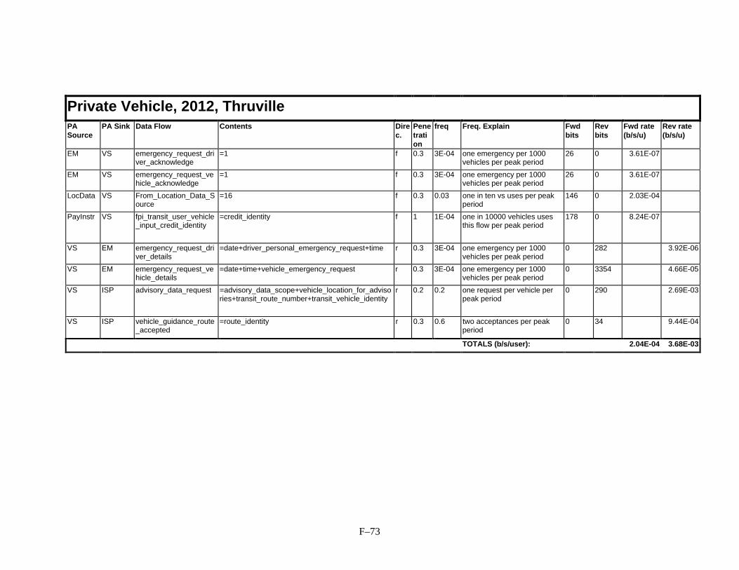
F–73
Private Vehicle, 2012, ThruvillePASource
PA Sink Data Flow Contents Direc.
Penetration
freq Freq. Explain Fwdbits
Revbits
Fwd rate(b/s/u)
Rev rate(b/s/u)
EM VS emergency_request_driver_acknowledge
=1 f 0.3 3E-04 one emergency per 1000vehicles per peak period
26 0 3.61E-07
EM VS emergency_request_vehicle_acknowledge
=1 f 0.3 3E-04 one emergency per 1000vehicles per peak period
26 0 3.61E-07
LocData VS From_Location_Data_Source
=16 f 0.3 0.03 one in ten vs uses per peakperiod
146 0 2.03E-04
PayInstr VS fpi_transit_user_vehicle_input_credit_identity
=credit_identity f 1 1E-04 one in 10000 vehicles usesthis flow per peak period
178 0 8.24E-07
VS EM emergency_request_driver_details
=date+driver_personal_emergency_request+time r 0.3 3E-04 one emergency per 1000vehicles per peak period
0 282 3.92E-06
VS EM emergency_request_vehicle_details
=date+time+vehicle_emergency_request r 0.3 3E-04 one emergency per 1000vehicles per peak period
0 3354 4.66E-05
VS ISP advisory_data_request =advisory_data_scope+vehicle_location_for_advisories+transit_route_number+transit_vehicle_identity
r 0.2 0.2 one request per vehicle perpeak period
0 290 2.69E-03
VS ISP vehicle_guidance_route_accepted
=route_identity r 0.3 0.6 two acceptances per peakperiod
0 34 9.44E-04
TOTALS (b/s/user): 2.04E-04 3.68E-03

F–74
Traveler, 2012, ThruvillePASource
PA Sink Data Flow Contents Direc.
Penetration
freq Freq. Explain Fwdbits
Revbits
Fwd rate(b/s/u)
Rev rate(b/s/u)
EM PIAS emergency_request_personal_traveler_acknowledge
=confirmation_flag f 0.3 8E-05 one emergency per 2000users in peak period
26 0 9.03E-08
ISP PIAS transit_deviations_for_portables
=traveler_identity+list_size+TRANSIT_SEGS*(transit_vehicle_identity+transit_vehicle_achieved_time+transit_route_segment_number)
f 0.2 5E-04 one request per 20 pias perpeak period
3578 0 8.28E-05
ISP PIAS traveler_guidance_route =route_identity+traveler_route+traveler_identity f 0.3 0.015 one route per day per pias 18306 0 1.27E-02
LocData PIAS From_Location_Data_Source
=16 f 0.3 0.03 one in ten pias uses per peakperiod
146 0 2.03E-04
PIAS EM emergency_request_personal_traveler_details
=date+time+traveler_personal_emergency_request r 0.3 8E-05 one emergency per 2000users in peak period
0 370 1.28E-06
PIAS ISP traffic_data_portables_request
=traffic_data_request+traveler_identity r 0.2 0.1 one request per pias per peakperiod
0 250 1.16E-03
PIAS ISP transit_deviations_portables_request
=traveler_identity+transit_vehicle_deviation_request+transit_route_number
r 0.2 0.005 one request per 20 pias perpeak period
0 250 5.79E-05
TOTALS (b/s/user): 1.30E-02 1.22E-03

F–75
CVO-Local, 2012, ThruvillePASource
PA Sink Data Flow Contents Direc.
Penetration
freq Freq. Explain Fwdbits
Revbits
Fwd rate(b/s/u)
Rev rate(b/s/u)
CVS FMS cf_driver_route_instructions_request
=cv_driver_number+cv_route_number r 0.8 1.6 average fleet vehicle requeststwo routes per peak period
0 154 5.70E-03
CVS FMS cv_driver_route_request =trip_request+route_type r 0.8 3.2 average vehicle requests 4routes per peak period
0 1234 9.14E-02
CVS FMS cv_driver_storage_request
=cv_route_number r 0.8 0.08 one in ten vehicles per peakperiod
0 26 4.81E-05
CVS FMS cv_static_route_data =256 r 0.8 3.2 four routes per vehicle perpeak period
0 2066 1.53E-01
EM FMS cf_hazmat_request =16 f 0.5 5E-05 once per 1000 vehicles perpeak period
146 0 1.69E-07
EM VS emergency_request_driver_acknowledge
=1 f 0.3 3E-04 one emergency per 1000vehicles per peak period
26 0 1.81E-07
EM VS emergency_request_vehicle_acknowledge
=1 f 0.3 3E-04 one emergency per 1000vehicles per peak period
26 0 1.81E-07
FMS CVS cf_driver_route_instructions
=cf_driver_route+cf_driver_load_details f 0.8 1.6 twice per vehicle per peakperiod
5082 0 1.88E-01
FMS CVS cv_driver_route_data =cv_route_data+route_type+cv_route_number f 0.8 3.2 average vehicle requests fourroutes per peak period
3042 0 2.25E-01
FMS CVS cv_static_route_request =origin+destination+departure_time+desired_arrival_time+preferences+constraints
f 0.8 3.2 average vehicle requests fourroutes per peak period
1226 0 9.08E-02
FMS EM cf_hazmat_route_information
=cv_route_number+route r 0.5 5E-05 once per 1000 vehicles perpeak period
0 3754 4.34E-06
FMS EM cf_hazmat_vehicle_information
=28 r 0.5 5E-05 once per 1000 vehicles perpeak period
0 242 2.80E-07
FMS ImFrghtD
To_Intermodal_Freight_Depot
=64 r 0.8 0.008 one in ten of vehicles interactonce with an intermodalcarrier
0 530 9.81E-05
FMS ImFrghtS To_Intermodal_Freight_Shipper
=64 r 0.8 0.008 one in ten of vehicles interactonce with an intermodalcarrier
0 530 9.81E-05

F–76
CVO-Local, 2012, ThruvilleFMS ISP cf_route_request =trip_request+cv_route_number r 0.8 0.16 twice per vehicle per peak
period0 1234 4.57E-03
FMS ISP cv_route_request =trip_request+vehicle_identity r 0.8 0.32 four times per vehicle perpeak period
0 1354 1.00E-02
ImFrghtD FMS From_Intermodal_Freight_Depot
=64 f 0.8 0.008 one in ten of vehicles interactonce with an intermodalcarrier
530 0 9.81E-05
ImFrghtS FMS From_Intermodal_Freight_Shipper
=64 f 0.8 0.008 one in ten of vehicles interactonce with an intermodalcarrier
530 0 9.81E-05
ISP FMS cf_route =cv_route_data+cv_route_number f 0.8 0.16 twice per vehicle per peakperiod
3034 0 1.12E-02
ISP FMS cv_route =cv_route_data+vehicle_identity f 0.8 0.32 four times per vehicle perpeak period
3154 0 2.34E-02
LocData VS From_Location_Data_Source
=16 f 0.3 0.03 one in ten vehicles uses onceper peak period
146 0 1.01E-04
VS EM emergency_request_driver_details
=date+driver_personal_emergency_request+time r 0.3 3E-04 one emergency per 1000vehicles per peak period
0 282 1.96E-06
VS EM emergency_request_vehicle_details
=date+time+vehicle_emergency_request r 0.3 3E-04 one emergency per 1000vehicles per peak period
0 3354 2.33E-05
VS ISP advisory_data_request =advisory_data_scope+vehicle_location_for_advisories+transit_route_number+transit_vehicle_identity
r 0.2 0.4 two requests per vehicle perpeak period
0 290 2.69E-03
TOTALS (b/s/user): 5.39E-01 2.68E-01

F–77
CVO-Long Haul, 2012, ThruvillePASource
PA Sink Data Flow Contents Direc.
Penetration
freq Freq. Explain Fwdbits
Revbits
Fwd rate(b/s/u)
Rev rate(b/s/u)
CVAS CVCS cv_credentials_database_update
=cv_credentials_details+cv_credentials_status_code+cv_trip_classification_data
f 0.85 9E-05 one out of 1000 vehicles perpeak period
482 0 9.48E-07
CVAS CVCS cv_credentials_information_response
=cv_credentials_details+cv_credentials_status_code
f 0.85 0.009 one out of 10 vehicles 410 0 8.07E-05
CVAS CVCS cv_safety_database_update
=cv_credentials_details+cv_roadside_safety_data f 1 0.001 one out of 100 vehicles 410 0 9.49E-06
CVAS CVCS cv_safety_information_response
=cv_credentials_details+cv_roadside_safety_data f 1 0.001 one out of 100 vehicles aretransmitted
410 0 9.49E-06
CVAS FMS cf_clearance_enrollment_confirm
=confirmation_flag f 0.85 0.085 once per vehicle per peakperiod
26 0 5.12E-05
CVAS FMS cf_enrollment_information
=cv_route_number+cv_taxes_and_duties+route+route_type
f 0.85 0.043 one out of two vehiclesrequire info. per peak period
3818 0 3.76E-03
CVAS FMS cf_enrollment_payment_confirmation
=cv_route_number+cv_account_number+cv_amount_billed
f 0.85 0.085 once per vehicle per peakperiod
170 0 3.34E-04
CVAS FMS cv_enrollment_information
=cv_route_number+cv_taxes_and_duties+route+route_type
f 0.85 0.043 one out of two vehiclesrequire info. per peak period
3818 0 3.76E-03
CVAS FMS cv_enrollment_payment_confirmation
=cv_account_number+cv_amount_billed+cv_driver_credit_identity+cv_route_number
f 0.85 0.085 once per vehicle per peakperiod
346 0 6.81E-04
CVCS CVAS cv_credentials_information_request
=cv_credentials_details+cv_credentials_request_type+cv_credentials_request_identity+cv_roadside_facility_identity
r 0.85 0.009 request info on one in tenvehicles
0 554 1.09E-04
CVCS CVAS cv_roadside_daily_log =cv_roadside_facility_identity+date++cv_archived_safety_data+cv_archived_inspection_data+cv_screening_record
r 0.85 9E-04 one report per 100 vehiclesper peak period
0 3362 6.62E-05
CVCS CVAS cv_safety_information_request
=cv_credentials_details+cv_safety_information_request_identity+cv_safety_information_request_type+cv_roadside_facility_identity
r 1 0.01 request info on one in tenvehicles
0 554 1.28E-04
CVCS CVAS cv_update_safety_problems_list
=cv_credentials_details+cv_roadside_facility_identity+cv_roadside_safety_data
r 1 0.001 one out of 100 vehicles areon the list per peak period
0 538 1.25E-05
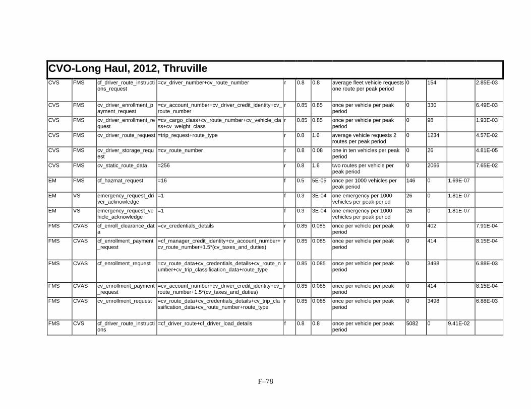
F–78
CVO-Long Haul, 2012, ThruvilleCVS FMS cf_driver_route_instructi
ons_request=cv_driver_number+cv_route_number r 0.8 0.8 average fleet vehicle requests
one route per peak period0 154 2.85E-03
CVS FMS cv_driver_enrollment_payment_request
=cv_account_number+cv_driver_credit_identity+cv_route_number
r 0.85 0.85 once per vehicle per peakperiod
0 330 6.49E-03
CVS FMS cv_driver_enrollment_request
=cv_cargo_class+cv_route_number+cv_vehicle_class+cv_weight_class
r 0.85 0.85 once per vehicle per peakperiod
0 98 1.93E-03
CVS FMS cv_driver_route_request =trip_request+route_type r 0.8 1.6 average vehicle requests 2routes per peak period
0 1234 4.57E-02
CVS FMS cv_driver_storage_request
=cv_route_number r 0.8 0.08 one in ten vehicles per peakperiod
0 26 4.81E-05
CVS FMS cv_static_route_data =256 r 0.8 1.6 two routes per vehicle perpeak period
0 2066 7.65E-02
EM FMS cf_hazmat_request =16 f 0.5 5E-05 once per 1000 vehicles perpeak period
146 0 1.69E-07
EM VS emergency_request_driver_acknowledge
=1 f 0.3 3E-04 one emergency per 1000vehicles per peak period
26 0 1.81E-07
EM VS emergency_request_vehicle_acknowledge
=1 f 0.3 3E-04 one emergency per 1000vehicles per peak period
26 0 1.81E-07
FMS CVAS cf_enroll_clearance_data
=cv_credentials_details r 0.85 0.085 once per vehicle per peakperiod
0 402 7.91E-04
FMS CVAS cf_enrollment_payment_request
=cf_manager_credit_identity+cv_account_number+cv_route_number+1.5*(cv_taxes_and_duties)
r 0.85 0.085 once per vehicle per peakperiod
0 414 8.15E-04
FMS CVAS cf_enrollment_request =cv_route_data+cv_credentials_details+cv_route_number+cv_trip_classification_data+route_type
r 0.85 0.085 once per vehicle per peakperiod
0 3498 6.88E-03
FMS CVAS cv_enrollment_payment_request
=cv_account_number+cv_driver_credit_identity+cv_route_number+1.5*(cv_taxes_and_duties)
r 0.85 0.085 once per vehicle per peakperiod
0 414 8.15E-04
FMS CVAS cv_enrollment_request =cv_route_data+cv_credentials_details+cv_trip_classification_data+cv_route_number+route_type
r 0.85 0.085 once per vehicle per peakperiod
0 3498 6.88E-03
FMS CVS cf_driver_route_instructions
=cf_driver_route+cf_driver_load_details f 0.8 0.8 once per vehicle per peakperiod
5082 0 9.41E-02

F–79
CVO-Long Haul, 2012, ThruvilleFMS CVS cv_driver_enrollment_in
formation=cv_route_number+cv_taxes_and_duties f 0.85 0.425 one out of two vehicles
require info. per peak period82 0 8.07E-04
FMS CVS cv_driver_enrollment_payment_confirmation
=cv_account_number+cv_amount_billed+cv_driver_credit_identity+cv_route_number
f 0.85 0.85 once per vehicle per peakperiod
346 0 6.81E-03
FMS CVS cv_driver_route_data =cv_route_data+route_type+cv_route_number f 0.8 1.6 average vehicle requests tworoutes per peak period
3042 0 1.13E-01
FMS CVS cv_static_route_request =origin+destination+departure_time+desired_arrival_time+preferences+constraints
f 0.8 1.6 average vehicle requests tworoutes per peak period
1226 0 4.54E-02
FMS EM cf_hazmat_route_information
=cv_route_number+route r 0.5 5E-05 once per 1000 vehicles perpeak period
0 3754 4.34E-06
FMS EM cf_hazmat_vehicle_information
=28 r 0.5 5E-05 once per 1000 vehicles perpeak period
0 242 2.80E-07
FMS ImFrghtD
To_Intermodal_Freight_Depot
=64 r 0.8 0.008 one in ten vehicles interactsonce with an intermodalcarrier
0 530 9.81E-05
FMS ImFrghtS To_Intermodal_Freight_Shipper
=64 r 0.8 0.008 one in ten vehicles interactsonce with an intermodalcarrier
0 530 9.81E-05
FMS ISP cf_route_request =trip_request+cv_route_number r 0.8 0.08 once per vehicle per peakperiod
0 1234 2.29E-03
FMS ISP cv_route_request =trip_request+vehicle_identity r 0.8 0.16 twice per vehicle per peakperiod
0 1354 5.01E-03
FMS PayInstr tpi_debited_commercial_manager_payment
=4 r 0.85 0.085 once per enrollment 0 50 9.84E-05
ImFrghtD FMS From_Intermodal_Freight_Depot
=64 f 0.8 0.008 one in ten vehicles interactsonce with an intermodalcarrier
530 0 9.81E-05
ImFrghtS FMS From_Intermodal_Freight_Shipper
=64 f 0.8 0.008 one in ten vehicles interactsonce with an intermodalcarrier
530 0 9.81E-05
ISP FMS cf_route =cv_route_data+cv_route_number f 0.8 0.08 once per vehicle per peakperiod
3034 0 5.62E-03
ISP FMS cv_route =cv_route_data+vehicle_identity f 0.8 0.16 twice per vehicle per peakperiod
3154 0 1.17E-02

F–80
CVO-Long Haul, 2012, ThruvilleLocData VS From_Location_Data_S
ource=16 f 0.3 0.03 one in ten vehicles uses once
per peak period146 0 1.01E-04
PayInstr FMS fpi_commercial_manager_input_credit_identity
=12 f 0.85 0.085 once per enrollment = onceper cv per peak period
114 0 2.24E-04
VS EM emergency_request_driver_details
=date+driver_personal_emergency_request+time r 0.3 3E-04 one emergency per 1000vehicles per peak period
0 282 1.96E-06
VS EM emergency_request_vehicle_details
=date+time+vehicle_emergency_request r 0.3 3E-04 one emergency per 1000vehicles per peak period
0 3354 2.33E-05
VS ISP advisory_data_request =advisory_data_scope+vehicle_location_for_advisories+transit_route_number+transit_vehicle_identity
r 0.2 0.4 two requests per vehicle perpeak period
0 290 2.69E-03
VS ISP vehicle_guidance_route_accepted
=route_identity r 0.3 0.6 two acceptances per peakperiod
0 34 4.72E-04
TOTALS (b/s/user): 2.86E-01 1.61E-01

F–81
Transit, 2012, ThruvillePASource
PA Sink Data Flow Contents Direc.
Penetration
freq Freq. Explain Fwdbits
Revbits
Fwd rate(b/s/u)
Rev rate(b/s/u)
PayInstr TRVS fpi_confirm_fare_payment_on_transit_vehicle
=confirmation_flag f 1 32 average of one use per transituser per peak period = 32 pertransit vehicle
26 0 1.78E-02
PayInstr TRVS fpi_transit_vehicle_tag_data
=credit_identity f 1 0.032 one data set for 1000 users =0.032 uses per transit vehicleper peak period
178 0 1.22E-04
RTS ISP traffic_data_kiosk_request
=kiosk_identity+traffic_data_request r 0.2 0.64 average of one use per transituser per peak period = 32 pertransit vehicle
0 98 1.34E-03
RTS ISP transit_deviation_kiosk_request
=kiosk_identity+transit_vehicle_deviation_request r 0.2 0.128 one in five transit users = 6.4per transit vehicle per peakperiod
0 66 1.81E-04
RTS ISP traveler_current_condition_request
=kiosk_identity r 0.2 0.64 average of one use per transituser per peak period = 32 pertransit vehicle
0 58 7.93E-04
TRMS TRVS approved_corrective_plan
=transit_route_corrections+transit_changes_in_stops+transit_changes_in_speed
f 1 0.1 one corrective message perten vehicles per peak period
8210 0 1.75E-02
TRMS TRVS confirm_vehicle_fare_payment
=confirmation_flag f 1 32 average of one use per transituser per peak period = 32 pertransit vehicle
26 0 1.78E-02
TRMS TRVS paratransit_transit_driver_instructions
=128 f 1 13 dispatch message every 15min. during peakperiod=48/4(ratio of paratr/trveh)
1042 0 2.89E-01
TRMS TRVS request_transit_user_image
=8 f 1 0.032 one image for 1000 users =0.032 uses per transit vehicleper peak period
82 0 5.61E-05
TRMS TRVS transit_services_for_corrections
=list_size+1*(2/NUM_TRANSIT_ROUTES)*(transit_services)
f 1 13 one correction per hour duringthe peak period
17260 0 4.79E+00

F–82
Transit, 2012, ThruvilleTRMS TRVS transit_services_for_eta =transit_route_number+transit_route_segment_list+
transit_route_stop_listf 1 52 update every 15 minutes
during the peak period7786 0 8.65E+00
TRMS TRVS transit_services_for_vehicle_fares
=transit_route_fare_data f 1 1 update daily during peakperiod
16826 0 3.60E-01
TRMS TRVS transit_vehicle_advanced_payment_response
=advanced_charges_confirm+advanced_tolls_confirm+confirmation_flag+transit_vehicle_identity
f 1 0.032 one data set for 1000 users =0.032 uses per transit vehicleper peak period
554 0 3.79E-04
TRMS TRVS transit_vehicle_fare_data
=transit_fares f 1 1 updated once per peak periodper transit vehicle
922 0 1.97E-02
TRMS TRVS transit_vehicle_fare_payment_debited
=confirmation_flag f 1 32 average of one use per transituser per peak period = 32 pertransit vehicle
26 0 1.78E-02
TRMS TRVS transit_vehicle_fare_payment_request
=transit_fare f 1 32 average of one use per transituser per peak period = 32 pertransit vehicle
34 0 2.32E-02
TRVS PayInstr tpi_debited_payment_on_transit_vehicle
=4 f 1 32 average of one use per transituser per peak period = 32 pertransit vehicle
50 0 3.42E-02
TRVS PayInstr tpi_request_fare_payment_on_transit_vehicle
=2 f 1 32 average of one use per transituser per peak period = 32 pertransit vehicle
34 0 2.32E-02
TRVS TRMS paratransit_transit_vehicle_availability
=1 r 1 13 avail. message every 15 min.during peak period=48/4(ratioof paratr/tr veh)
0 26 7.22E-03
TRVS TRMS request_vehicle_fare_payment
=credit_identity+transit_fare+transit_route_number+transit_route_segment_number+transit_route_use_time+transit_user_category+traveler_identity
r 1 32 average of one use per peakperiod per transit user = 32per transit vehicle
0 466 3.19E-01
TRVS TRMS transit_conditions_request
=2 r 1 0.1 one corrective message perten vehicles per peak period
0 34 7.26E-05
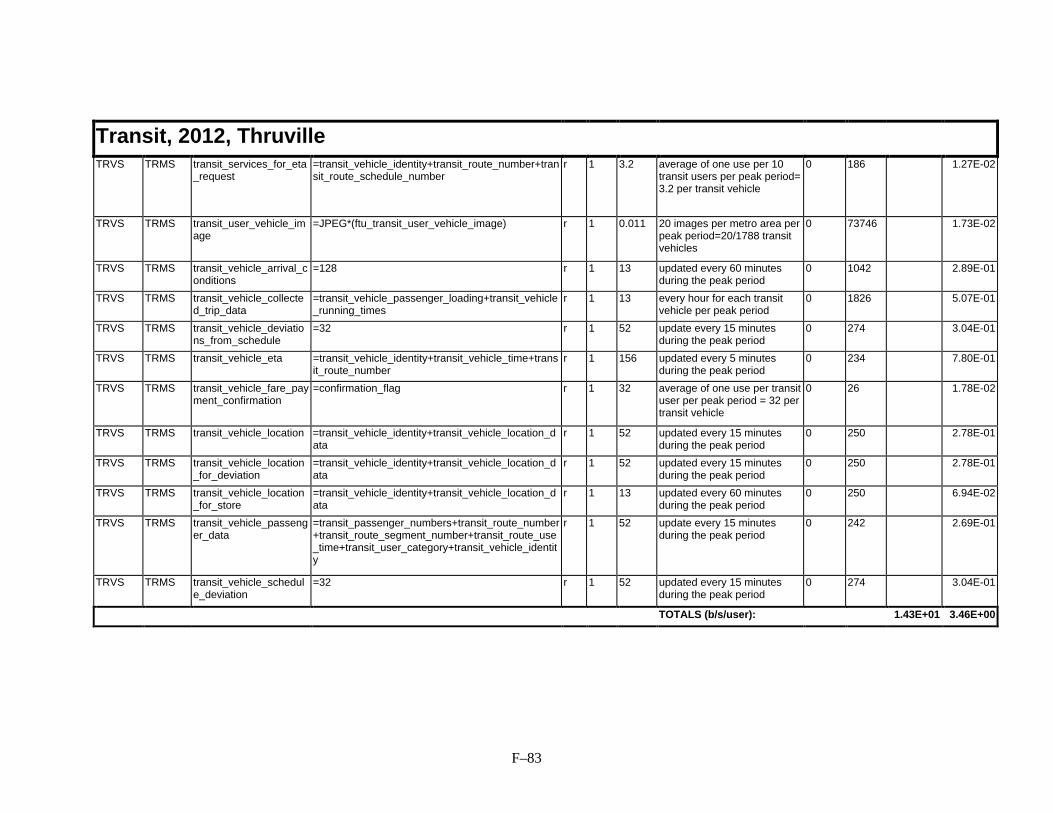
F–83
Transit, 2012, ThruvilleTRVS TRMS transit_services_for_eta
_request=transit_vehicle_identity+transit_route_number+transit_route_schedule_number
r 1 3.2 average of one use per 10transit users per peak period=3.2 per transit vehicle
0 186 1.27E-02
TRVS TRMS transit_user_vehicle_image
=JPEG*(ftu_transit_user_vehicle_image) r 1 0.011 20 images per metro area perpeak period=20/1788 transitvehicles
0 73746 1.73E-02
TRVS TRMS transit_vehicle_arrival_conditions
=128 r 1 13 updated every 60 minutesduring the peak period
0 1042 2.89E-01
TRVS TRMS transit_vehicle_collected_trip_data
=transit_vehicle_passenger_loading+transit_vehicle_running_times
r 1 13 every hour for each transitvehicle per peak period
0 1826 5.07E-01
TRVS TRMS transit_vehicle_deviations_from_schedule
=32 r 1 52 update every 15 minutesduring the peak period
0 274 3.04E-01
TRVS TRMS transit_vehicle_eta =transit_vehicle_identity+transit_vehicle_time+transit_route_number
r 1 156 updated every 5 minutesduring the peak period
0 234 7.80E-01
TRVS TRMS transit_vehicle_fare_payment_confirmation
=confirmation_flag r 1 32 average of one use per transituser per peak period = 32 pertransit vehicle
0 26 1.78E-02
TRVS TRMS transit_vehicle_location =transit_vehicle_identity+transit_vehicle_location_data
r 1 52 updated every 15 minutesduring the peak period
0 250 2.78E-01
TRVS TRMS transit_vehicle_location_for_deviation
=transit_vehicle_identity+transit_vehicle_location_data
r 1 52 updated every 15 minutesduring the peak period
0 250 2.78E-01
TRVS TRMS transit_vehicle_location_for_store
=transit_vehicle_identity+transit_vehicle_location_data
r 1 13 updated every 60 minutesduring the peak period
0 250 6.94E-02
TRVS TRMS transit_vehicle_passenger_data
=transit_passenger_numbers+transit_route_number+transit_route_segment_number+transit_route_use_time+transit_user_category+transit_vehicle_identity
r 1 52 update every 15 minutesduring the peak period
0 242 2.69E-01
TRVS TRMS transit_vehicle_schedule_deviation
=32 r 1 52 updated every 15 minutesduring the peak period
0 274 3.04E-01
TOTALS (b/s/user): 1.43E+01 3.46E+00
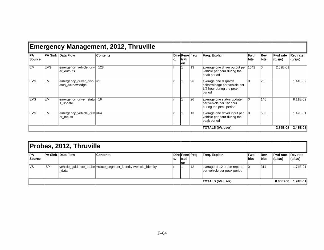
F–84
Emergency Management, 2012, ThruvillePASource
PA Sink Data Flow Contents Direc.
Penetration
freq Freq. Explain Fwdbits
Revbits
Fwd rate(b/s/u)
Rev rate(b/s/u)
EM EVS emergency_vehicle_driver_outputs
=128 f 1 13 average one driver output pervehicle per hour during thepeak period
1042 0 2.89E-01
EVS EM emergency_driver_dispatch_acknowledge
=1 r 1 26 average one dispatchacknowledge per vehicle per1/2 hour during the peakperiod
0 26 1.44E-02
EVS EM emergency_driver_status_update
=16 r 1 26 average one status updateper vehicle per 1/2 hourduring the peak period
0 146 8.11E-02
EVS EM emergency_vehicle_driver_inputs
=64 r 1 13 average one driver input pervehicle per hour during thepeak period
0 530 1.47E-01
TOTALS (b/s/user): 2.89E-01 2.43E-01
Probes, 2012, ThruvillePASource
PA Sink Data Flow Contents Direc.
Penetration
freq Freq. Explain Fwdbits
Revbits
Fwd rate(b/s/u)
Rev rate(b/s/u)
VS ISP vehicle_guidance_probe_data
=route_segment_identity+vehicle_identity r 1 12 average of 12 probe reportsper vehicle per peak period
0 314 1.74E-01
TOTALS (b/s/user): 0.00E+00 1.74E-01

F–85
Private Vehicle, 2012, MountainvillePASource
PA Sink Data Flow Contents Direc.
Penetration
freq Freq. Explain Fwdbits
Revbits
Fwd rate(b/s/u)
Rev rate(b/s/u)
EM VS emergency_request_driver_acknowledge
=1 f 0.3 3E-04 one emergency per 1000vehicles per peak period
26 0 3.61E-07
EM VS emergency_request_vehicle_acknowledge
=1 f 0.3 3E-04 one emergency per 1000vehicles per peak period
26 0 3.61E-07
ISP VS advanced_fares_and_charges_response
=confirmation_flag+credit_identity+parking_lot_cost+stored_credit+transit_fare
f 0.2 2E-04 one user per 1000 users perpeak period
234 0 2.17E-06
ISP VS advanced_tolls_and_fares_response
=confirmation_flag+credit_identity+stored_credit+toll_cost+transit_fare
f 0.2 2E-04 one user per 1000 users perpeak period
234 0 2.17E-06
ISP VS advisory_data =traffic_data_for_advisories+predicted_incidents_for_advisories+prediction_data_for_advisories+transit_services_for_advisories+transit_running_data_for_advisories
f 0.2 0.2 one set of data per peakperiod
6146 0 5.69E-02
ISP VS yellow_pages_advisory_data
=yellow_pages_data_for_advisories+yellow_pages_cost+yellow_pages_dining_reservation_confirmation+yellow_pages_lodging_reservation_confirmation+yellow_pages_ticket_purchase_confirmation
f 0.2 0.02 one yellow pages advisoryper 10 vehicles per peakperiod
10802 0 1.00E-02
LocData VS From_Location_Data_Source
=16 f 0.3 0.03 one in ten vs uses per peakperiod
146 0 2.03E-04
PayInstr VS fpi_driver_vehicle_input_credit_identity
=credit_identity f 0.2 2E-04 one vehicle per 1000 perpeak period
178 0 1.65E-06
PayInstr VS fpi_transit_user_vehicle_input_credit_identity
=credit_identity f 1 1E-04 one in 10000 vehicles usesthis flow per peak period
178 0 8.24E-07
VS EM emergency_request_driver_details
=date+driver_personal_emergency_request+time r 0.3 3E-04 one emergency per 1000vehicles per peak period
0 282 3.92E-06
VS EM emergency_request_vehicle_details
=date+time+vehicle_emergency_request r 0.3 3E-04 one emergency per 1000vehicles per peak period
0 3354 4.66E-05
VS ISP advanced_fares_and_charges_request
=0.6*(advanced_fare_details)+0.6*(advanced_parking_lot_charges)
r 0.2 2E-04 one user per 1000 users perpeak period
0 632.4 5.86E-06
VS ISP advanced_tolls_and_fares_request
=0.6*(advanced_fare_details)+0.6*(advanced_tolls) r 0.2 2E-04 one user per 1000 users perpeak period
0 642 5.94E-06

F–86
Private Vehicle, 2012, MountainvilleVS ISP advisory_data_request =advisory_data_scope+vehicle_location_for_adviso
ries+transit_route_number+transit_vehicle_identityr 0.2 0.2 one request per vehicle per
peak period0 290 2.69E-03
VS ISP vehicle_guidance_route_accepted
=route_identity r 0.3 0.6 two acceptances per peakperiod
0 34 9.44E-04
VS ISP yellow_pages_advisory_requests
=advisory_data_scope+vehicle_location_for_advisories+transit_route_number+transit_vehicle_identity+yellow_pages_dining_reservation+yellow_pages_lodging_reservation+yellow_pages_ticket_purchase
r 0.2 0.02 one yellow pages advisoryper ten vehicles per peakperiod
0 674 6.24E-04
VS PayInstr tpi_debited_driver_payment_at_vehicle
=4 r 0.2 2E-04 one vehicle per 1000 perpeak period
0 50 4.63E-07
VS PMS advanced_parking_lot_charges_request
=credit_identity+parking_lot_identity+parking_space_details+stored_credit+vehicle_identity
r 0.2 1E-04 one user per 1000 users perpeak period
0 514 2.38E-06
VS PMS parking_lot_payment_confirmation
=confirmation_flag r 0.2 1E-04 one vehicle per 1000 perpeak period
0 26 1.20E-07
TOTALS (b/s/user): 6.71E-02 4.32E-03

F–87
Traveler, 2012, MountainvillePASource
PA Sink Data Flow Contents Direc.
Penetration
freq Freq. Explain Fwdbits
Revbits
Fwd rate(b/s/u)
Rev rate(b/s/u)
EM PIAS emergency_request_personal_traveler_acknowledge
=confirmation_flag f 0.3 8E-05 one emergency per 2000users in peak period
26 0 9.03E-08
ISP PIAS transit_deviations_for_portables
=traveler_identity+list_size+TRANSIT_SEGS*(transit_vehicle_identity+transit_vehicle_achieved_time+transit_route_segment_number)
f 0.2 5E-04 one request per 20 pias perpeak period
3578 0 8.28E-05
ISP PIAS traveler_guidance_route =route_identity+traveler_route+traveler_identity f 0.3 0.015 one route per day per pias 18306 0 1.27E-02
ISP PIAS traveler_personal_payment_confirmation
=advanced_tolls_confirm+advanced_fares_confirm+advanced_parking_lot_charges_confirm+credit_identity+stored_credit+traveler_identity+traveler_total_trip_cost
f 0.2 0.01 one payment per 10 pias perpeak period
818 0 3.79E-04
ISP PIAS traveler_personal_transaction_confirmation
=credit_identity+traveler_identity+transaction_number+yellow_pages_cost+yellow_pages_lodging_reservation_confirmation+yellow_pages_dining_reservation_confirmation+yellow_pages_ticket_purchase_confirmation
f 0.2 0.01 one confirmation per 10 piasper day
650 0 3.01E-04
ISP PIAS traveler_personal_yellow_pages_data
=traveler_identity+0.01*(yellow_pages_general_information+yellow_pages_specific_information+yellow_pages_transaction_information)
f 0.2 0.1 one yellow pages responseper pias per peak period
1140 0 5.28E-03
LocData PIAS From_Location_Data_Source
=16 f 0.3 0.03 one in ten pias uses per peakperiod
146 0 2.03E-04
PayInstr PIAS fpi_traveler_personal_input_credit_identity
=credit_identity f 0.2 0.01 one transaction per 10 piasper day
178 0 8.24E-05
PIAS EM emergency_request_personal_traveler_details
=date+time+traveler_personal_emergency_request r 0.3 8E-05 one emergency per 2000users in peak period
0 370 1.28E-06
PIAS ISP traffic_data_portables_request
=traffic_data_request+traveler_identity r 0.2 0.1 one request per pias per peakperiod
0 250 1.16E-03
PIAS ISP transit_deviations_portables_request
=traveler_identity+transit_vehicle_deviation_request+transit_route_number
r 0.2 0.005 one request per 20 pias perpeak period
0 250 5.79E-05

F–88
Traveler, 2012, MountainvillePIAS ISP traveler_personal_curre
nt_condition_request=traveler_identity r 0.2 0.1 one request per pias per peak
period0 210 9.72E-04
PIAS ISP traveler_personal_payment_information
=credit_identity+parking_space_details+ride_segments+stored_credit+toll_segments+traveler_identity
r 0.2 0.01 one payment per 10 pias perpeak period
0 1130 5.23E-04
PIAS ISP traveler_personal_transaction_request
=yellow_pages_dining_reservation+yellow_pages_lodging_reservation+yellow_pages_ticket_purchase
r 0.2 0.01 one request per 10 pias perpeak period
0 402 1.86E-04
PIAS ISP traveler_personal_yellow_pages_information_request
=1 r 0.2 0.1 one yellow pages request perpias per peak period
0 26 1.20E-04
PIAS PayInstr tpi_debited_payment_at_personal_device
=4 r 0.2 0.01 one transaction per 10 piasper day
0 50 2.31E-05
PIAS TRMS transit_services_portables_request
=destination+origin+traveler_identity r 0.2 0.01 one request per 10 pias perpeak period
0 466 2.16E-04
TRMS PIAS transit_services_for_portables
=traveler_identity+2*(transit_services_for_output) f 0.2 0.003 one request per 20 pias perpeak period
2530 0 3.87E-04
TOTALS (b/s/user): 1.94E-02 3.26E-03

F–89
CVO-Local, 2012, MountainvillePASource
PA Sink Data Flow Contents Direc.
Penetration
freq Freq. Explain Fwdbits
Revbits
Fwd rate(b/s/u)
Rev rate(b/s/u)
CVS FMS cf_driver_route_instructions_request
=cv_driver_number+cv_route_number r 0.8 1.6 average fleet vehicle requeststwo routes per peak period
0 154 5.70E-03
CVS FMS cf_on_board_vehicle_data
=cv_on_board_data+cv_general_output_message+vehicle_location_for_cv
r 0.1 0.2 two times per vehicle perpeak period for an averageover all vehicles
0 2106 9.75E-03
CVS FMS cv_driver_route_request =trip_request+route_type r 0.8 3.2 average vehicle requests 4routes per peak period
0 1234 9.14E-02
CVS FMS cv_driver_storage_request
=cv_route_number r 0.8 0.08 one in ten vehicles per peakperiod
0 26 4.81E-05
CVS FMS cv_static_route_data =256 r 0.8 3.2 four routes per vehicle perpeak period
0 2066 1.53E-01
EM FMS cf_hazmat_request =16 f 0.5 5E-05 once per 1000 vehicles perpeak period
146 0 1.69E-07
EM VS emergency_request_driver_acknowledge
=1 f 0.3 3E-04 one emergency per 1000vehicles per peak period
26 0 1.81E-07
EM VS emergency_request_vehicle_acknowledge
=1 f 0.3 3E-04 one emergency per 1000vehicles per peak period
26 0 1.81E-07
FMS CVS cf_driver_route_instructions
=cf_driver_route+cf_driver_load_details f 0.8 1.6 twice per vehicle per peakperiod
5082 0 1.88E-01
FMS CVS cf_request_on_board_vehicle_data
=2 f 0.1 0.4 four times per vehicle perpeak period for an averageover all vehicles
34 0 3.15E-04
FMS CVS cv_driver_route_data =cv_route_data+route_type+cv_route_number f 0.8 3.2 average vehicle requests fourroutes per peak period
3042 0 2.25E-01
FMS CVS cv_static_route_request =origin+destination+departure_time+desired_arrival_time+preferences+constraints
f 0.8 3.2 average vehicle requests fourroutes per peak period
1226 0 9.08E-02
FMS EM cf_hazmat_route_information
=cv_route_number+route r 0.5 5E-05 once per 1000 vehicles perpeak period
0 3754 4.34E-06
FMS EM cf_hazmat_vehicle_information
=28 r 0.5 5E-05 once per 1000 vehicles perpeak period
0 242 2.80E-07

F–90
CVO-Local, 2012, MountainvilleFMS ImFrght
DTo_Intermodal_Freight_Depot
=64 r 0.8 0.008 one in ten of vehicles interactonce with an intermodalcarrier
0 530 9.81E-05
FMS ImFrghtS To_Intermodal_Freight_Shipper
=64 r 0.8 0.008 one in ten of vehicles interactonce with an intermodalcarrier
0 530 9.81E-05
FMS ISP cf_route_request =trip_request+cv_route_number r 0.8 0.16 twice per vehicle per peakperiod
0 1234 4.57E-03
FMS ISP cv_route_request =trip_request+vehicle_identity r 0.8 0.32 four times per vehicle perpeak period
0 1354 1.00E-02
ImFrghtD FMS From_Intermodal_Freight_Depot
=64 f 0.8 0.008 one in ten of vehicles interactonce with an intermodalcarrier
530 0 9.81E-05
ImFrghtS FMS From_Intermodal_Freight_Shipper
=64 f 0.8 0.008 one in ten of vehicles interactonce with an intermodalcarrier
530 0 9.81E-05
ISP FMS cf_route =cv_route_data+cv_route_number f 0.8 0.16 twice per vehicle per peakperiod
3034 0 1.12E-02
ISP FMS cv_route =cv_route_data+vehicle_identity f 0.8 0.32 four times per vehicle perpeak period
3154 0 2.34E-02
ISP VS advanced_fares_and_charges_response
=confirmation_flag+credit_identity+parking_lot_cost+stored_credit+transit_fare
f 0.2 2E-04 one user per 1000 users perpeak period
234 0 1.08E-06
ISP VS advanced_tolls_and_fares_response
=confirmation_flag+credit_identity+stored_credit+toll_cost+transit_fare
f 0.2 2E-04 one user per 1000 users perpeak period
234 0 1.08E-06
ISP VS advisory_data =traffic_data_for_advisories+predicted_incidents_for_advisories+prediction_data_for_advisories+transit_services_for_advisories+transit_running_data_for_advisories
f 0.2 0.4 two sets of data per peakperiod
6146 0 5.69E-02
ISP VS yellow_pages_advisory_data
=yellow_pages_data_for_advisories+yellow_pages_cost+yellow_pages_dining_reservation_confirmation+yellow_pages_lodging_reservation_confirmation+yellow_pages_ticket_purchase_confirmation
f 0.2 0.02 one yellow pages advisoryper 10 vehicles per peakperiod
10802 0 5.00E-03
LocData VS From_Location_Data_Source
=16 f 0.3 0.03 one in ten vehicles uses onceper peak period
146 0 1.01E-04

F–91
CVO-Local, 2012, MountainvillePayInstr VS fpi_driver_vehicle_input
_credit_identity=credit_identity f 0.2 2E-04 one vehicle per 1000 per
peak period178 0 8.24E-07
VS EM emergency_request_driver_details
=date+driver_personal_emergency_request+time r 0.3 3E-04 one emergency per 1000vehicles per peak period
0 282 1.96E-06
VS EM emergency_request_vehicle_details
=date+time+vehicle_emergency_request r 0.3 3E-04 one emergency per 1000vehicles per peak period
0 3354 2.33E-05
VS ISP advanced_fares_and_charges_request
=0.6*(advanced_fare_details)+0.6*(advanced_parking_lot_charges)
r 0.2 2E-04 one user per 1000 users perpeak period
0 632.4 2.93E-06
VS ISP advanced_tolls_and_fares_request
=0.6*(advanced_fare_details)+0.6*(advanced_tolls) r 0.2 2E-04 one user per 1000 users perpeak period
0 642 2.97E-06
VS ISP advisory_data_request =advisory_data_scope+vehicle_location_for_advisories+transit_route_number+transit_vehicle_identity
r 0.2 0.4 two requests per vehicle perpeak period
0 290 2.69E-03
VS ISP yellow_pages_advisory_requests
=advisory_data_scope+vehicle_location_for_advisories+transit_route_number+transit_vehicle_identity+yellow_pages_dining_reservation+yellow_pages_lodging_reservation+yellow_pages_ticket_purchase
r 0.2 0.02 one yellow pages advisoryper 10 vehicles per peakperiod
0 674 3.12E-04
VS PayInstr tpi_debited_driver_payment_at_vehicle
=4 r 0.2 2E-04 one vehicle per 1000 perpeak period
0 50 2.31E-07
VS PMS advanced_parking_lot_charges_request
=credit_identity+parking_lot_identity+parking_space_details+stored_credit+vehicle_identity
r 0.2 1E-04 one user per 1000 users perpeak period
0 514 1.19E-06
VS PMS parking_lot_payment_confirmation
=confirmation_flag r 0.2 1E-04 one vehicle per 1000 perpeak period
0 26 6.02E-08
TOTALS (b/s/user): 6.01E-01 2.78E-01

F–92
CVO-Long Haul, 2012, MountainvillePASource
PA Sink Data Flow Contents Direc.
Penetration
freq Freq. Explain Fwdbits
Revbits
Fwd rate(b/s/u)
Rev rate(b/s/u)
CVAS CVCS cv_credentials_database_update
=cv_credentials_details+cv_credentials_status_code+cv_trip_classification_data
f 0.85 9E-05 one out of 1000 vehicles perpeak period
482 0 9.48E-07
CVAS CVCS cv_credentials_information_response
=cv_credentials_details+cv_credentials_status_code
f 0.85 0.009 one out of 10 vehicles 410 0 8.07E-05
CVAS CVCS cv_safety_database_update
=cv_credentials_details+cv_roadside_safety_data f 1 0.001 one out of 100 vehicles 410 0 9.49E-06
CVAS CVCS cv_safety_information_response
=cv_credentials_details+cv_roadside_safety_data f 1 0.001 one out of 100 vehicles aretransmitted
410 0 9.49E-06
CVAS FMS cf_clearance_enrollment_confirm
=confirmation_flag f 0.85 0.085 once per vehicle per peakperiod
26 0 5.12E-05
CVAS FMS cf_enrollment_information
=cv_route_number+cv_taxes_and_duties+route+route_type
f 0.85 0.043 one out of two vehiclesrequire info. per peak period
3818 0 3.76E-03
CVAS FMS cf_enrollment_payment_confirmation
=cv_route_number+cv_account_number+cv_amount_billed
f 0.85 0.085 once per vehicle per peakperiod
170 0 3.34E-04
CVAS FMS cv_enrollment_information
=cv_route_number+cv_taxes_and_duties+route+route_type
f 0.85 0.043 one out of two vehiclesrequire info. per peak period
3818 0 3.76E-03
CVAS FMS cv_enrollment_payment_confirmation
=cv_account_number+cv_amount_billed+cv_driver_credit_identity+cv_route_number
f 0.85 0.085 once per vehicle per peakperiod
346 0 6.81E-04
CVCS CVAS cv_credentials_information_request
=cv_credentials_details+cv_credentials_request_type+cv_credentials_request_identity+cv_roadside_facility_identity
r 0.85 0.009 request info on one in tenvehicles
0 554 1.09E-04
CVCS CVAS cv_roadside_daily_log =cv_roadside_facility_identity+date++cv_archived_safety_data+cv_archived_inspection_data+cv_screening_record
r 0.85 9E-04 one report per 100 vehiclesper peak period
0 3362 6.62E-05
CVCS CVAS cv_safety_information_request
=cv_credentials_details+cv_safety_information_request_identity+cv_safety_information_request_type+cv_roadside_facility_identity
r 1 0.01 request info on one in tenvehicles
0 554 1.28E-04
CVCS CVAS cv_update_safety_problems_list
=cv_credentials_details+cv_roadside_facility_identity+cv_roadside_safety_data
r 1 0.001 one out of 100 vehicles areon the list per peak period
0 538 1.25E-05
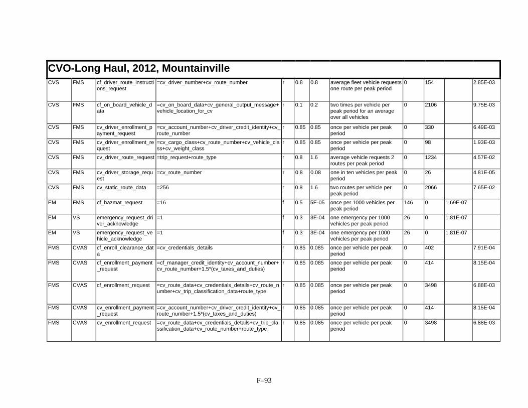
F–93
CVO-Long Haul, 2012, MountainvilleCVS FMS cf_driver_route_instructi
ons_request=cv_driver_number+cv_route_number r 0.8 0.8 average fleet vehicle requests
one route per peak period0 154 2.85E-03
CVS FMS cf_on_board_vehicle_data
=cv_on_board_data+cv_general_output_message+vehicle_location_for_cv
r 0.1 0.2 two times per vehicle perpeak period for an averageover all vehicles
0 2106 9.75E-03
CVS FMS cv_driver_enrollment_payment_request
=cv_account_number+cv_driver_credit_identity+cv_route_number
r 0.85 0.85 once per vehicle per peakperiod
0 330 6.49E-03
CVS FMS cv_driver_enrollment_request
=cv_cargo_class+cv_route_number+cv_vehicle_class+cv_weight_class
r 0.85 0.85 once per vehicle per peakperiod
0 98 1.93E-03
CVS FMS cv_driver_route_request =trip_request+route_type r 0.8 1.6 average vehicle requests 2routes per peak period
0 1234 4.57E-02
CVS FMS cv_driver_storage_request
=cv_route_number r 0.8 0.08 one in ten vehicles per peakperiod
0 26 4.81E-05
CVS FMS cv_static_route_data =256 r 0.8 1.6 two routes per vehicle perpeak period
0 2066 7.65E-02
EM FMS cf_hazmat_request =16 f 0.5 5E-05 once per 1000 vehicles perpeak period
146 0 1.69E-07
EM VS emergency_request_driver_acknowledge
=1 f 0.3 3E-04 one emergency per 1000vehicles per peak period
26 0 1.81E-07
EM VS emergency_request_vehicle_acknowledge
=1 f 0.3 3E-04 one emergency per 1000vehicles per peak period
26 0 1.81E-07
FMS CVAS cf_enroll_clearance_data
=cv_credentials_details r 0.85 0.085 once per vehicle per peakperiod
0 402 7.91E-04
FMS CVAS cf_enrollment_payment_request
=cf_manager_credit_identity+cv_account_number+cv_route_number+1.5*(cv_taxes_and_duties)
r 0.85 0.085 once per vehicle per peakperiod
0 414 8.15E-04
FMS CVAS cf_enrollment_request =cv_route_data+cv_credentials_details+cv_route_number+cv_trip_classification_data+route_type
r 0.85 0.085 once per vehicle per peakperiod
0 3498 6.88E-03
FMS CVAS cv_enrollment_payment_request
=cv_account_number+cv_driver_credit_identity+cv_route_number+1.5*(cv_taxes_and_duties)
r 0.85 0.085 once per vehicle per peakperiod
0 414 8.15E-04
FMS CVAS cv_enrollment_request =cv_route_data+cv_credentials_details+cv_trip_classification_data+cv_route_number+route_type
r 0.85 0.085 once per vehicle per peakperiod
0 3498 6.88E-03

F–94
CVO-Long Haul, 2012, MountainvilleFMS CVS cf_driver_route_instructi
ons=cf_driver_route+cf_driver_load_details f 0.8 0.8 once per vehicle per peak
period5082 0 9.41E-02
FMS CVS cf_request_on_board_vehicle_data
=2 f 0.1 0.2 two times per vehicle perpeak period for an averageover all vehicles
34 0 1.57E-04
FMS CVS cv_driver_enrollment_information
=cv_route_number+cv_taxes_and_duties f 0.85 0.425 one out of two vehiclesrequire info. per peak period
82 0 8.07E-04
FMS CVS cv_driver_enrollment_payment_confirmation
=cv_account_number+cv_amount_billed+cv_driver_credit_identity+cv_route_number
f 0.85 0.85 once per vehicle per peakperiod
346 0 6.81E-03
FMS CVS cv_driver_route_data =cv_route_data+route_type+cv_route_number f 0.8 1.6 average vehicle requests tworoutes per peak period
3042 0 1.13E-01
FMS CVS cv_static_route_request =origin+destination+departure_time+desired_arrival_time+preferences+constraints
f 0.8 1.6 average vehicle requests tworoutes per peak period
1226 0 4.54E-02
FMS EM cf_hazmat_route_information
=cv_route_number+route r 0.5 5E-05 once per 1000 vehicles perpeak period
0 3754 4.34E-06
FMS EM cf_hazmat_vehicle_information
=28 r 0.5 5E-05 once per 1000 vehicles perpeak period
0 242 2.80E-07
FMS ImFrghtD
To_Intermodal_Freight_Depot
=64 r 0.8 0.008 one in ten vehicles interactsonce with an intermodalcarrier
0 530 9.81E-05
FMS ImFrghtS To_Intermodal_Freight_Shipper
=64 r 0.8 0.008 one in ten vehicles interactsonce with an intermodalcarrier
0 530 9.81E-05
FMS ISP cf_route_request =trip_request+cv_route_number r 0.8 0.08 once per vehicle per peakperiod
0 1234 2.29E-03
FMS ISP cv_route_request =trip_request+vehicle_identity r 0.8 0.16 twice per vehicle per peakperiod
0 1354 5.01E-03
FMS PayInstr tpi_debited_commercial_manager_payment
=4 r 0.85 0.085 once per enrollment 0 50 9.84E-05
ImFrghtD FMS From_Intermodal_Freight_Depot
=64 f 0.8 0.008 one in ten vehicles interactsonce with an intermodalcarrier
530 0 9.81E-05

F–95
CVO-Long Haul, 2012, MountainvilleImFrghtS FMS From_Intermodal_Freig
ht_Shipper=64 f 0.8 0.008 one in ten vehicles interacts
once with an intermodalcarrier
530 0 9.81E-05
ISP FMS cf_route =cv_route_data+cv_route_number f 0.8 0.08 once per vehicle per peakperiod
3034 0 5.62E-03
ISP FMS cv_route =cv_route_data+vehicle_identity f 0.8 0.16 twice per vehicle per peakperiod
3154 0 1.17E-02
ISP VS advanced_fares_and_charges_response
=confirmation_flag+credit_identity+parking_lot_cost+stored_credit+transit_fare
f 0.2 2E-04 one user per 1000 users perpeak period
234 0 1.08E-06
ISP VS advanced_tolls_and_fares_response
=confirmation_flag+credit_identity+stored_credit+toll_cost+transit_fare
f 0.2 2E-04 one user per 1000 users perpeak period
234 0 1.08E-06
ISP VS advisory_data =traffic_data_for_advisories+predicted_incidents_for_advisories+prediction_data_for_advisories+transit_services_for_advisories+transit_running_data_for_advisories
f 0.2 0.2 one set of data per peakperiod
6146 0 2.85E-02
ISP VS yellow_pages_advisory_data
=yellow_pages_data_for_advisories+yellow_pages_cost+yellow_pages_dining_reservation_confirmation+yellow_pages_lodging_reservation_confirmation+yellow_pages_ticket_purchase_confirmation
f 0.2 0.02 one yellow pages advisoryper 10 vehicles per peakperiod
10802 0 5.00E-03
LocData VS From_Location_Data_Source
=16 f 0.3 0.03 one in ten vehicles uses onceper peak period
146 0 1.01E-04
PayInstr FMS fpi_commercial_manager_input_credit_identity
=12 f 0.85 0.085 once per enrollment = onceper cv per peak period
114 0 2.24E-04
PayInstr VS fpi_driver_vehicle_input_credit_identity
=credit_identity f 0.2 2E-04 one vehicle per 1000 perpeak period
178 0 8.24E-07
VS EM emergency_request_driver_details
=date+driver_personal_emergency_request+time r 0.3 3E-04 one emergency per 1000vehicles per peak period
0 282 1.96E-06
VS EM emergency_request_vehicle_details
=date+time+vehicle_emergency_request r 0.3 3E-04 one emergency per 1000vehicles per peak period
0 3354 2.33E-05
VS ISP advanced_fares_and_charges_request
=0.6*(advanced_fare_details)+0.6*(advanced_parking_lot_charges)
r 0.2 2E-04 one user per 1000 users perpeak period
0 632.4 2.93E-06
VS ISP advanced_tolls_and_fares_request
=0.6*(advanced_fare_details)+0.6*(advanced_tolls) r 0.2 2E-04 one user per 1000 users perpeak period
0 642 2.97E-06

F–96
CVO-Long Haul, 2012, MountainvilleVS ISP advisory_data_request =advisory_data_scope+vehicle_location_for_adviso
ries+transit_route_number+transit_vehicle_identityr 0.2 0.4 two requests per vehicle per
peak period0 290 2.69E-03
VS ISP vehicle_guidance_route_accepted
=route_identity r 0.3 0.6 two acceptances per peakperiod
0 34 4.72E-04
VS ISP yellow_pages_advisory_requests
=advisory_data_scope+vehicle_location_for_advisories+transit_route_number+transit_vehicle_identity+yellow_pages_dining_reservation+yellow_pages_lodging_reservation+yellow_pages_ticket_purchase
r 0.2 0.02 one yellow pages advisoryper 10 vehicles per peakperiod
0 674 3.12E-04
VS PayInstr tpi_debited_driver_payment_at_vehicle
=4 r 0.2 2E-04 one vehicle per 1000 perpeak period
0 50 2.31E-07
VS PMS advanced_parking_lot_charges_request
=credit_identity+parking_lot_identity+parking_space_details+stored_credit+vehicle_identity
r 0.2 1E-04 one user per 1000 users perpeak period
0 514 1.19E-06
VS PMS parking_lot_payment_confirmation
=confirmation_flag r 0.2 1E-04 one vehicle per 1000 perpeak period
0 26 6.02E-08
TOTALS (b/s/user): 3.20E-01 1.71E-01
Transit, 2012, MountainvillePASource
PA Sink Data Flow Contents Direc.
Penetration
freq Freq. Explain Fwdbits
Revbits
Fwd rate(b/s/u)
Rev rate(b/s/u)
ISP RTS advanced_tolls_and_charges_roadside_confirm
=advanced_charges_confirm+advanced_tolls_confirm+confirmation_flag
f 0.2 6E-04 one use per 1000 transitusers per peak period, or0.032/transit vehicle
426 0 5.83E-06
ISP RTS traveler_payment_confirmation
=advanced_tolls_confirm+advanced_fares_confirm+advanced_parking_lot_charges_confirm+credit_identity+kiosk_identity+stored_credit+traveler_total_trip_cost
f 0.2 6E-04 one use per 1000 transitusers per peak period, or0.032/transit vehicle
666 0 9.11E-06
ISP RTS traveler_transaction_confirmation
=credit_identity+kiosk_identity+transaction_number+yellow_pages_cost+yellow_pages_lodging_reservation_confirmation+yellow_pages_dining_reservation_confirmation+yellow_pages_ticket_purchase_confirmation
f 0.2 6E-04 one use per 1000 transitusers per peak period, or0.032/transit vehicle
498 0 6.81E-06

F–97
Transit, 2012, MountainvilleISP RTS traveler_yellow_pages_
data=kiosk_identity+0.01*(yellow_pages_general_information+yellow_pages_specific_information+yellow_pages_transaction_information)
f 0.2 6E-04 one use per 1000 transitusers per peak period, or0.032/transit vehicle
987.7 0 1.35E-05
PayInstr RTS fpi_confirm_fare_payment_at_roadside
=confirmation_flag f 0.2 0.128 one in five transit users = 6.4per transit vehicle per peakperiod
26 0 7.11E-05
PayInstr RTS fpi_transit_roadside_tag_data
=credit_identity f 0.2 6E-04 one data set for 1000 users =0.032 uses per transit vehicleper peak period
178 0 2.43E-06
PayInstr RTS fpi_transit_user_roadside_input_credit_identity
=credit_identity f 0.2 6E-04 one data set for 1000 users =0.032 uses per transit vehicleper peak period
178 0 2.43E-06
PayInstr RTS fpi_traveler_roadside_input_credit_identity
=credit_identity f 0.2 6E-04 one data set for 1000 users =0.032 uses per transit vehicleper peak period
178 0 2.43E-06
PayInstr TRVS fpi_confirm_fare_payment_on_transit_vehicle
=confirmation_flag f 1 32 average of one use per transituser per peak period = 32 pertransit vehicle
26 0 1.78E-02
PayInstr TRVS fpi_transit_vehicle_tag_data
=credit_identity f 1 0.032 one data set for 1000 users =0.032 uses per transit vehicleper peak period
178 0 1.22E-04
RTS EM emergency_request_kiosk_traveler_details
=date+time+traveler_personal_emergency_request r 1 0.003 one emergency per 1000transit users per peak period,or 0.032/transit vehicle
0 370 2.53E-05
RTS ISP advanced_tolls_and_charges_roadside_request
=0.6*(advanced_charges)+0.6*(advanced_tolls) r 0.2 6E-04 one use per 1000 transitusers per peak period, or0.032/transit vehicle
0 738 1.01E-05
RTS ISP traffic_data_kiosk_request
=kiosk_identity+traffic_data_request r 0.2 0.64 average of one use per transituser per peak period = 32 pertransit vehicle
0 98 1.34E-03
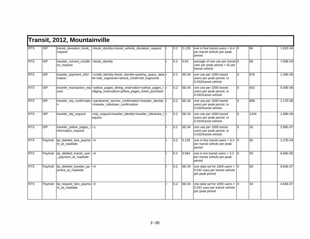
F–98
Transit, 2012, MountainvilleRTS ISP transit_deviation_kiosk_
request=kiosk_identity+transit_vehicle_deviation_request r 0.2 0.128 one in five transit users = 6.4
per transit vehicle per peakperiod
0 66 1.81E-04
RTS ISP traveler_current_condition_request
=kiosk_identity r 0.2 0.64 average of one use per transituser per peak period = 32 pertransit vehicle
0 58 7.93E-04
RTS ISP traveler_payment_information
=credit_identity+kiosk_identity+parking_space_details+ride_segments+stored_credit+toll_segments
r 0.2 6E-04 one use per 1000 transitusers per peak period, or0.032/transit vehicle
0 978 1.34E-05
RTS ISP traveler_transaction_request
=yellow_pages_dining_reservation+yellow_pages_lodging_reservation+yellow_pages_ticket_purchase
r 0.2 6E-04 one use per 1000 transitusers per peak period, or0.032/transit vehicle
0 402 5.50E-06
RTS ISP traveler_trip_confirmation
=paratransit_service_confirmation+traveler_identity+traveler_rideshare_confirmation
r 0.2 6E-04 one use per 1000 transitusers per peak period, or0.032/transit vehicle
0 858 1.17E-05
RTS ISP traveler_trip_request =trip_request+traveler_identity+traveler_rideshare_request
r 0.2 6E-04 one use per 1000 transitusers per peak period, or0.032/transit vehicle
0 1434 1.96E-05
RTS ISP traveler_yellow_pages_information_request
=1 r 0.2 6E-04 one use per 1000 transitusers per peak period, or0.032/transit vehicle
0 26 3.56E-07
RTS PayInstr tpi_debited_fare_payment_at_roadside
=4 r 0.2 0.128 one in five transit users = 6.4per transit vehicle per peakperiod
0 50 1.37E-04
RTS PayInstr tpi_debited_transit_user_payment_at_roadside
=4 r 0.2 0.064 one in ten transit users = 3.2per transit vehicle per peakperiod
0 50 6.84E-05
RTS PayInstr tpi_debited_traveler_payment_at_roadside
=4 r 0.2 6E-04 one data set for 1000 users =0.032 uses per transit vehicleper peak period
0 50 6.84E-07
RTS PayInstr tpi_request_fare_payment_at_roadside
=2 r 0.2 6E-04 one data set for 1000 users =0.032 uses per transit vehicleper peak period
0 34 4.65E-07

F–99
Transit, 2012, MountainvilleTRMS TRVS approved_corrective_pl
an=transit_route_corrections+transit_changes_in_stops+transit_changes_in_speed
f 1 0.1 one corrective message perten vehicles per peak period
8210 0 1.75E-02
TRMS TRVS confirm_vehicle_fare_payment
=confirmation_flag f 1 32 average of one use per transituser per peak period = 32 pertransit vehicle
26 0 1.78E-02
TRMS TRVS other_services_vehicle_response
=traveler_identity+credit_identity+other_services_data
f 0.2 0.006 one data set for 1000 users =0.032 uses per transit vehicleper peak period
2418 0 3.31E-04
TRMS TRVS paratransit_transit_driver_instructions
=128 f 1 13 dispatch message every 15min. during peakperiod=48/4(ratio of paratr/trveh)
1042 0 2.89E-01
TRMS TRVS request_transit_user_image
=8 f 1 0.032 one image for 1000 users =0.032 uses per transit vehicleper peak period
82 0 5.61E-05
TRMS TRVS transit_operator_request_acknowledge
=2 f 1 0.032 one data set for 1000 users =0.032 uses per transit vehicleper peak period
34 0 2.32E-05
TRMS TRVS transit_services_for_corrections
=list_size+1*(2/NUM_TRANSIT_ROUTES)*(transit_services)
f 1 13 one correction per hour duringthe peak period
17260 0 4.79E+00
TRMS TRVS transit_services_for_eta =transit_route_number+transit_route_segment_list+transit_route_stop_list
f 1 52 update every 15 minutesduring the peak period
7786 0 8.65E+00
TRMS TRVS transit_services_for_vehicle_fares
=transit_route_fare_data f 1 1 update daily during peakperiod
16826 0 3.60E-01
TRMS TRVS transit_vehicle_advanced_payment_response
=advanced_charges_confirm+advanced_tolls_confirm+confirmation_flag+transit_vehicle_identity
f 1 0.032 one data set for 1000 users =0.032 uses per transit vehicleper peak period
554 0 3.79E-04
TRMS TRVS transit_vehicle_fare_data
=transit_fares f 1 1 updated once per peak periodper transit vehicle
922 0 1.97E-02
TRMS TRVS transit_vehicle_fare_payment_debited
=confirmation_flag f 1 32 average of one use per transituser per peak period = 32 pertransit vehicle
26 0 1.78E-02

F–100
Transit, 2012, MountainvilleTRMS TRVS transit_vehicle_fare_pay
ment_request=transit_fare f 1 32 average of one use per transit
user per peak period = 32 pertransit vehicle
34 0 2.32E-02
TRVS PayInstr tpi_debited_payment_on_transit_vehicle
=4 f 1 32 average of one use per transituser per peak period = 32 pertransit vehicle
50 0 3.42E-02
TRVS PayInstr tpi_request_fare_payment_on_transit_vehicle
=2 f 1 32 average of one use per transituser per peak period = 32 pertransit vehicle
34 0 2.32E-02
TRVS TRMS other_services_vehicle_request
=traveler_identity+credit_identity+other_services_data
r 0.2 0.006 one data set for 1000 users =0.032 uses per transit vehicleper peak period
0 2418 3.31E-04
TRVS TRMS paratransit_transit_vehicle_availability
=1 r 1 13 avail. message every 15 min.during peak period=48/4(ratioof paratr/tr veh)
0 26 7.22E-03
TRVS TRMS request_vehicle_fare_payment
=credit_identity+transit_fare+transit_route_number+transit_route_segment_number+transit_route_use_time+transit_user_category+traveler_identity
r 1 32 average of one use per peakperiod per transit user = 32per transit vehicle
0 466 3.19E-01
TRVS TRMS transit_conditions_request
=2 r 1 0.1 one corrective message perten vehicles per peak period
0 34 7.26E-05
TRVS TRMS transit_emergency_details
=transit_driver_emergency_request+transit_user_emergency_request+transit_vehicle_location
r 1 0.003 emergency for one in 10000transit users=0.0032 pertransit vehicle per peak
0 282 1.93E-05
TRVS TRMS transit_emergency_information
=transit_driver_emergency_request+transit_user_emergency_request+transit_vehicle_location
r 1 0.003 emergency for one in 10000transit users=0.0032 pertransit vehicle per peak
0 282 1.93E-05
TRVS TRMS transit_operator_emergency_request
=128 r 1 0.003 emergency for one in 10000transit users=0.0032 pertransit vehicle per peak
0 1042 7.12E-05

F–101
Transit, 2012, MountainvilleTRVS TRMS transit_services_for_eta
_request=transit_vehicle_identity+transit_route_number+transit_route_schedule_number
r 1 3.2 average of one use per 10transit users per peak period=3.2 per transit vehicle
0 186 1.27E-02
TRVS TRMS transit_user_vehicle_image
=JPEG*(ftu_transit_user_vehicle_image) r 1 0.011 20 images per metro area perpeak period=20/1788 transitvehicles
0 73746 1.73E-02
TRVS TRMS transit_vehicle_advanced_payment_request
=advanced_charges+advanced_tolls+transit_vehicle_location
r 0.2 0.006 one data set for 1000 users =0.032 uses per transit vehicleper peak period
0 1450 1.98E-04
TRVS TRMS transit_vehicle_arrival_conditions
=128 r 1 13 updated every 60 minutesduring the peak period
0 1042 2.89E-01
TRVS TRMS transit_vehicle_collected_trip_data
=transit_vehicle_passenger_loading+transit_vehicle_running_times
r 1 13 every hour for each transitvehicle per peak period
0 1826 5.07E-01
TRVS TRMS transit_vehicle_deviations_from_schedule
=32 r 1 52 update every 15 minutesduring the peak period
0 274 3.04E-01
TRVS TRMS transit_vehicle_eta =transit_vehicle_identity+transit_vehicle_time+transit_route_number
r 1 156 updated every 5 minutesduring the peak period
0 234 7.80E-01
TRVS TRMS transit_vehicle_fare_payment_confirmation
=confirmation_flag r 1 32 average of one use per transituser per peak period = 32 pertransit vehicle
0 26 1.78E-02
TRVS TRMS transit_vehicle_location =transit_vehicle_identity+transit_vehicle_location_data
r 1 52 updated every 15 minutesduring the peak period
0 250 2.78E-01
TRVS TRMS transit_vehicle_location_for_deviation
=transit_vehicle_identity+transit_vehicle_location_data
r 1 52 updated every 15 minutesduring the peak period
0 250 2.78E-01
TRVS TRMS transit_vehicle_location_for_store
=transit_vehicle_identity+transit_vehicle_location_data
r 1 13 updated every 60 minutesduring the peak period
0 250 6.94E-02
TRVS TRMS transit_vehicle_passenger_data
=transit_passenger_numbers+transit_route_number+transit_route_segment_number+transit_route_use_time+transit_user_category+transit_vehicle_identity
r 1 52 update every 15 minutesduring the peak period
0 242 2.69E-01
TRVS TRMS transit_vehicle_schedule_deviation
=32 r 1 52 updated every 15 minutesduring the peak period
0 274 3.04E-01
TOTALS (b/s/user): 1.43E+01 3.46E+00

F–102
Emergency Management, 2012, MountainvillePASource
PA Sink Data Flow Contents Direc.
Penetration
freq Freq. Explain Fwdbits
Revbits
Fwd rate(b/s/u)
Rev rate(b/s/u)
EM EVS emergency_vehicle_driver_outputs
=128 f 1 13 average one driver output pervehicle per hour during thepeak period
1042 0 2.89E-01
EVS EM emergency_driver_dispatch_acknowledge
=1 r 1 26 average one dispatchacknowledge per vehicle per1/2 hour during the peakperiod
0 26 1.44E-02
EVS EM emergency_driver_status_update
=16 r 1 26 average one status updateper vehicle per 1/2 hourduring the peak period
0 146 8.11E-02
EVS EM emergency_vehicle_driver_inputs
=64 r 1 13 average one driver input pervehicle per hour during thepeak period
0 530 1.47E-01
TOTALS (b/s/user): 2.89E-01 2.43E-01

G–1
APPENDIX G USE OF BEACONS FOR WIDE AREA
DELIVERY /COLLECTION OF ITS I NFORMATION
G.1 Introduction
In the ITS architecture, certain ITS interconnections are handled by means of wide area wirelesscommunication systems such as cellular, while other services are handled by short range wirelesslinks such as dedicated short range communications (DSRC) systems or beacons. It is importantto chose the communications technology appropriate for each application. It is also worthwhile toobserve that ITS has a number of new applications for each technology that will expand the useof existing infrastructures. Significant attention has been paid to the wide area technologyelsewhere in this document. This section focuses more on the dedicated short rangecommunications. The broad collection of messages specific to this interface is summarized intable G5.1.
The first type of interconnections, wide area wireless communication systems, supports severalservice groupings which include:
• traveler and driver information (e.g., routes, yellow pages information, emergency services)
• commercial vehicle operation – local and long haul (e.g., routes, dispatch, preclearance,yellow pages, emergency services, vehicle and cargo tracking)
• emergency vehicle management (e.g., dispatch, routes, status reporting)
The second type of interconnections, short range wireless links, support services that include:
• public transportation management (e.g., fixed route and paratransit management, emergencyservices, fare and passenger load management)
• toll collection
• roadside safety inspection (e.g., roadside check and safety check)
• in-vehicle signing (e.g., fixed signage beacons, incident warning beacons)
Message structure, traffic loading, and performance have been analyzed elsewhere in thisdocument for the first type of interconnections under the proposed cell-based architecture.However, the partition of user services between wide-area and short-range wirelesscommunication is not uniquely determined by (technical) system requirements.
In the communications analysis, messages are allowed to flow over the wide area (u1t) interfaceand the dedicated short range (u2) interface. A determination of the fraction that may flow overeach interface was also made. The assignments are detailed in Section 4.5 of this document.

G–2
Table 4.5-1 lists the messages and the interface(s) that each is allowed to flow over. This tablewas primarily developed in order to model the u1t interface loads, and therefore was designed forthe worst case analysis for that interface. This means that the ratio of u1t to u2 data loads waskept high, and u1t data loads were maximized by assuming that the use of the u2 interface doesnot, in many cases, reduce the u1t data load. This was done in order to model the worst casesituation where no beacons are deployed.
The purpose of this section is to examine, primarily from technical and feasibility standpoints,alternative architectures in which some or all of the services in the first category are provided byshort-range wireless communication between vehicles and roadside beacons, i.e., wide areacoverage by means of roadside beacons. The specific beacon system considered here just as anexample is Hughes’ DSRC system.
Three technical issues will be examined quantitatively, based on traffic loading analyses whichhave already been performed. These are: 1) compatibility of message formats with Hughes’signaling format used here as a working example; 2) the impact of DSRC data traffic on thewireline network; and 3) most importantly, the crucial issue of coverage and the related problemsof delay and complexity. Conclusions will then be drawn, from a technical perspective, regardingthe utilization of short-range communication systems (beacons) in the ITS architecture. This willbe followed by an analysis that touches upon the economic considerations of wide areadeployment of dedicated beacon systems.
G.2 Candidate Beacon Deployment
All beacons in the metropolitan area are assumed to use the same frequency, and beaconplacement is constrained by the need to eliminate interference. In the DSRC system, receiversensitivity is set to limit the effective range to about 200 feet. For acceptable interference levels,the minimum separation between beacons in the absence of obstructions is about 1/3 mile. Thisleads to the deployment shown below using cross-hatched circles. In an urban or suburbansetting, however, the obstruction caused by buildings located on a rectangular street grid allowsplacement of additional beacons without interference. Typically the number of beacons can bedoubled by locating the additional beacons (shown as dotted circles) equidistant from the originalones. We therefore postulate the idealized full deployment of Figure G.2-1.
1/3 mile
radius=200 ft
1/3
mile
Figure G.2-1 Full Deployment of a Beacon System

G–3
In this deployment, there are eighteen beacons per square mile. Since the Urbansville regioncovers 800 square miles, the postulated deployment would require approximately 14,400beacons. The postulated full deployment of DSRC would greatly increase the number of deviceswhich must be installed along roadways and connected via wired communication networksrelative to a cellular wide area solution, and would thus increase the initial costs associated withcommunication infrastructure deployment.
Another key aspect of the indicated deployment is that the fraction of the total area actuallywithin communication range of a beacon is just 18 * π(200)2 / 52802 = 0.081 (8.1%). However,given that the vehicles move essentially on surface streets and highways, it is more meaningful tocompute the percentage of “linear” coverage, i.e., the fraction of the roadway length covered bythe beacons. The fraction is slightly higher at 200 / (5280/3) = 0.114 (11.4%). This immediatelypoints out to the fact that only a small percentage of the vehicles will be within range of such afully deployed system.
This possible coverage could be increased if frequency reuse were implemented, since beaconsoperating at different frequencies could be interspersed among those shown above. Such asystem would then be no different from a full fledged micro-cellular system-- and if implementedon a wide scale as in the case of cellular telephone systems, would be prohibitively expensivefor any dedicated set of users . Such a hypothetical situation, however, would defeat the essenceof DSRC, which is based on site specific information exchange. Thus, it will not be considered.
G.3 Message Compatibility with DSRC
Again we consider here the open system specification proposed by Hughes as an example of aDSRC system capabilities. The Hughes system uses TDMA with a reservation slotted-ALOHAaccess protocol to resolve collisions that result from multiple vehicles responding to the triggerof the reader. The TDMA protocol has a basic frame length of 9.58 ms (including guard and deadtimes) during which the reader and transponders communicate. The frame consists of threesegments. The first is the segment where the reader sends a control message to activate thetransponders and/or give them instructions. The second segment is the data message segmentcontaining four slots each of which can be used for either forward or reverse transmission of adata packet under control of the reader. The size of these packets is 512 bits. The third segment isthe one in which transponders respond to the reader's trigger with their respective ID's.
The message lengths which have been defined in the ITS architecture to be sent over the u2interface for various wireless ITS services are generally less than 500 bits. (See Table G.5-1 for alisting of the messages.) Hence, the majority of ITS messages will be compatible with a single512 bit slot in the DSRC TDMA format. In some cases, messages may include larger amounts ofdata that will significantly increase their length. However, these messages can be accommodatedeither by multiple slots within a frame or multiple slots in successive frames.
G.4 Impact of ITS Data on Beacon Capacity
The effective user data rate of a beacon (on the order of 200 kbps) is much greater than that of amobile wide area wireless channel (e.g., a CDPD channel with a 19.2 kbps channel rate). Inaddition, a beacon will serve fewer vehicles than a cellular sector. Therefore, data throughput ofa DSRC is adequate to support ITS wireless traffic from vehicles within its limited range (100 to200 feet).

G–4
G.5 Impact of DSRC Traffic on Wireline Network
If wide area wireless communication is based on beacons rather than cell-based techniques,additional communications loading will occur on the wireline network connecting beacons, hubsand TMCs. In a cell-based architecture, wide area mobile communications are provided bywireless carriers, so they do not contribute to this wireline traffic. If cellular communicationswere replaced by widely deployed beacons, some of this wireless traffic would also have to passthrough the ITS wireline network.
Many beacons may be placed along highway rights of way and then be able to utilize any privatefiber network placed along that path to provide wireline communications with their controller.
The larger fraction of the total beacon population that is not along a fiber route will need to beconnected to the beacon controller through additional wireline links. These will be assumed to beleased digital lines and will not impact the performance of any existing wireline network..

G–5
Table G.5-1 ITS Wireless Messages for the u2 Interface
PA Source PA Sink Logical Data Flow Size (Bytes)Basic Vehicle PMS fbv vehicle characteristics 6Basic Vehicle RS fbv vehicle characteristics 6Basic Vehicle TCS fbv vehicle characteristics 6Commercial Vehicle CVCS fcv vehicle characteristics 6CVCS Commercial Vehicle
Drivertcvd clearance pull in output 64
CVCS Commercial VehicleDriver
tcvd general pull in output 64
CVCS Commercial VehicleDriver
tcvd safety pull in output 64
CVCS Commercial VehicleDriver
tcvd inspection results 32
CVCS CVS cv inspection data output 1024CVCS CVS cv request on board data 32CVS CVCS cv on board data 200CVS CVCS cv electronic clearance data 48EVS RS emergency vehicle preemptions 8PMS Driver td parking lot payment confirmed 2PMS Driver td parking lot payment invalid 2PMS VS parking lot payment debited 1PMS VS parking lot payment request 2PMS VS advanced parking lot charges confirm 18Potential Obstacles VS From Potential Obstacles 16Roadway VS From Roadway 16Roadway VS From Roadway 16RS Driver td lane use indication 4RS Driver td ramp state indication 4RS Driver td signal indication 4RS Driver td vms indication 8RS VS vehicle signage data 20RS VS ahs check response 513TCS Driver td toll payment confirmed 2TCS Driver td toll payment invalid 2TCS VS toll payment debited 1TCS VS toll payment request 2TRMS Transit Driver ttd route assignments 64TRMS TRVS transit operator request acknowledge 2TRMS TRVS approved corrective plan 1024TRMS TRVS transit vehicle conditions 2908TRMS TRVS paratransit transit driver instructions 128TRMS TRVS transit services for corrections 10240000TRMS TRVS transit services for eta 10240000TRMS TRVS transit vehicle advanced payment response 53TRMS TRVS transit vehicle fare payment debited 1TRMS TRVS transit vehicle fare payment request 2TRMS TRVS transit vehicle fare data 113TRMS TRVS request transit user image 8TRMS TRVS other services vehicle response 293TRMS TRVS transit services for vehicle fares 10240000TRMS TRVS confirm vehicle fare payment 1TRVS Payment Instrument tpi debited payment on transit vehicle 4TRVS Payment Instrument tpi request fare payment on transit vehicle 2TRVS RS transit roadway preemptions 16TRVS RS transit ramp preemptions 16TRVS TRMS transit emergency details 36TRVS TRMS transit operator emergency request 256TRVS TRMS transit user vehicle image 1024000TRVS TRMS fare collection vehicle violation information 1024046TRVS TRMS request vehicle fare payment 49

G–6
Table G.5-1 ITS Wireless Messages for the u2 Interface
PA Source PA Sink Logical Data Flow Size (Bytes)TRVS TRMS other services vehicle request 293TRVS TRMS transit vehicle passenger data 28TRVS TRMS paratransit transit vehicle availability 1TRVS TRMS transit vehicle fare payment confirmation 1TRVS TRMS transit vehicle advanced payment request 283TRVS TRMS transit vehicle location for deviation 32TRVS TRMS transit vehicle location 32TRVS TRMS transit vehicle arrival conditions 128TRVS TRMS transit vehicle schedule deviation 32TRVS TRMS transit vehicle eta 27TRVS TRMS transit vehicle deviations from schedule 32TRVS TRMS transit conditions request 2TRVS TRMS transit vehicle collected data 0TRVS TRMS transit emergency information 36TRVS TRMS transit vehicle location for store 32VehicleCharacteristics
PMS From Vehicle Characteristics 1000000
VehicleCharacteristics
TCS From Vehicle Characteristics 1000000
VS PMS parking lot payment confirmation 1VS PMS parking lot tag data 15VS PMS advanced parking lot charges request 74VS RS vehicle status details 4VS RS ahs route data 2401VS RS ahs vehicle condition 128VS TCS toll tag data 15VS TCS toll payment confirmation 1
G.6 Some Problems with Beacon Systems
One of the serious drawbacks of wireless communication using beacons is transmission delayswhich occur while a vehicle is located in the dead zone between beacons. This is, of course, mostsignificant for vehicles which are traveling slowly or are stationary for some period of time asillustrated in Figure G.6-1.
Vehicle Velocity (mph)
0
20
40
60
80
100
120
140
160
180
200
5
10 15 20 25 30 35 40 45 50 55 60 65 70 75 80 85 90 9510
0
Figure G.6-1 Transmission Delay as a Function of Vehicle Velocity

G–7
For example, a vehicle traveling 10 mph requires 93 seconds to traverse the 1360 foot dead zonebetween beacons. This should be compared with the following list of requirements for round-triptransmission time:
Driver information 5 secondsEn route transit advisory 5 secondsRoute guidance 5 secondsIncident management 1 secondTraffic control 5 secondsCommercial vehicle pre clearance 5 secondsAutomated roadside safety inspection 5 secondsCommercial vehicle administrative processing 5 secondsOn-board safety monitoring 5 secondsCommercial fleet management 15 secondsPublic transportation management 5 secondsPersonalized public transit 5 secondsEmergency notification and personal security 1 secondPublic travel security 1 secondEmergency vehicle management 1 second
It is clear that a beacon system cannot meet transmission time requirements for many wide areaITS services under normal traffic conditions.
Another problem that surfaces with a wide area deployment of a beacon system is the complexityrequired to carry out two-way communications between the fixed center (ISP or TMC) andvehicles which move from one beacon to another during the exchange. The time a movingvehicle will remain in the coverage area of a beacon is plotted in Figure G.6-2.
For example, a vehicle traveling at 60 mph will traverse beacon coverage (400 feet) in 4.6seconds. For many traffic types a query from the vehicle will elicit a response from either theTMC or a third-party provider. In many cases, the response will not be available until after thevehicle has left the coverage range of the beacon. Therefore, the TMC must direct its response tomultiple neighboring beacons. Figure G.6-3 shows the number of beacons at which vehiclestraveling at 60 mph might be located as a function of elapsed time assuming vehicle direction isknown to the service provider within ± 90 degrees. Compensating for this location uncertaintywill increase processing at the TMC or service provider and message storage at the beacons. Inorder to minimize wireless traffic, the beacon-to-vehicle communication protocol should restricttransmission of such responses to the first reader which establishes contact with the vehicle andtransmits the response.

G–8
Vehicle Velocity (mph)
0
10
20
30
40
50
60
510 15 20 25 30 35 40 45 50 55 60 65 70 75 80 85 90 95
100
Figure G.6-2 Time a Vehicle will Remain in the Coverage Area of a Beacon
Elapsed Time (sec)
0
5
10
15
20
25
30
35
0
10 20 30 40 50 60
Figure G.6-3 Location Uncertainty (number of beacons at which vehicles traveling at 60mph might be located at) as a Function of Elapsed Time

G–9
G.7 Summary
An evaluation of beacon systems in the context of providing wide area ITS communicationservices has led to the following conclusions:
• A widely deployed beacon system would be technically capable of accommodating projectedITS wireless communications traffic within its footprint. Such a beacon system wouldhowever be inadequate and inappropriate for all time-sensitive wide area services due toholes in coverage.
• A beacon system is appropriate only for specific short-range services, requiring only alimited deployment. This avoids issues of delay, complexity and above all cost, which arisein connection with a widely deployed system. Examples of short-range services for whichbeacons are suitable include toll collection, truck clearance at borders, and roadsideinspection (see Chapter 3 for the full details).

H–1
APPENDIX H WIRELESS AND WIRELINE PROTOCOLS
H.1 Wireless Protocols
H.1.1 CDPD
The wireless protocols for the CDPD test case are described concisely as follows:
1. Media access protocol: – DSMA/CD in the reverse link – TDM broadcast in the forward link
2. Link access protocol: MDLP
3. Error control/correction protocol: RS-coding plus TCP/IP control
4. Transport protocol: TCP
5. Networking protocols: IP
6. Routing algorithm/tables: IP
7. Packet processing algorithm: SNDCP
H.1.2 CDPD Protocols as Implemented in MOSS
The data delivery air-interface platform which is implemented on MOSS, follows the CellularDigital Packet Data (CDPD) reverse and forward links protocols. The following is a shortdescription of the CDPD part in MOSS, which draws closely from the CDPD systemspecification1.
In the forward link, MOSS implements a constantly transmitting Mobile Data Base Station(MDBS). By default, for a given base station and a given sector, MOSS randomly selects a singlechannel for CDPD use, out of the set of frequencies allocated to that sector under a given, mostlikely 3-sectored, frequency plan1.
1 The default frequency plan used in MOSS, which meets the Advanced Mobile Phone System (AMPS)
specifications, is given in Mobile Telecommunications Systems, W.C.Y. Lee, McGraw-Hill 1989.

H–2
MOSS’ CDPD forward link transmission information includes periodically two signals thatinform the mobile users on the reverse CDPD channel status: a "Busy/Idle" flag and a "DecodeStatus" flag. The content of these signals is constantly updated and is made available to the usercommunity every seven CDPD "minislots" (a minislot last 3.1msec approximately), i.e., everyRS-Block, the “quantum” of information in the reverse link. Note that no other information(more specifically no ITS information) is transmitted to the users in the forward link.
The performance of CDPD equipped cellular infrastructure for a mix of voice and data usershinges on the combined performance of the Physical layer and the Medium Access Control(MAC) layer on top of it. The task of the Physical layer design is to control the interferenceinduced by co-channel voice users in other cells through the use of power control and errorcorrecting codes (ECC), in this case a Reed-Solomon (RS) (63,47) code. The MAC protocol, onthe other hand, resolves contention on the common reverse channel due to the competition withthe other data users within the same cell.
In the reverse link, MOSS implements the random-access protocol as described in the CDPDSystem Specification. At the Physical Layer, the implementation uses independently computedresults regarding the decoding performance of a CDPD receiver that meets the specifications.The CDPD receiver uses a two-branch diversity scheme called Decision-Directed PhaseEstimation2. The receiver makes maximum use of knowledge of the waveform structure, and ofall the information made available by the system (e.g., the sync and continuity indications on thereverse link, and sync words and flags on the forward link).
At the MAC layer, MOSS follows all the details of CDPD reverse channel random-accessprotocol, which conforms to a non-persistent Digital Sense Multiple Access with CollisionDetection (DSMA/CD) protocol. Parts of the Mobile Data Link Protocol (MDLP) which relate tothe CDPD re-transmission policy are implemented as well.
The CDPD specification (see Figure H.1-1 and H.1-2) establishes the Reed-Solomon (RS)-blockas the quantum of information transmitted in the channel. Thus, the transaction lengthsdetermined elsewhere in this document have to be converted to the corresponding number ofblocks, taking into account the overhead introduced by TCP/IP.3 In its present form, TCP/IP adds40 bytes (320 bits) of addressing and control overhead to the first packet of each transaction. Ifmore than one packet (are required, significant header compression gain (from 40 to 3 bytes onaverage4) could be achieved. Industry consensus at this time is that four RS-blocks is theoptimum length of a packet. In the ITS case, all the transactions analyzed so far require only onepacket in each direction, so no gain can be achieved.
2 Described in Digital Communications, J.G. Proakis, McGraw-Hill, 1983.3 A recent reference on this subject is TCP/IP Illustrated- Volume I : The Protocols, W.R. Stevens,
Addison-Wesley, 1994.4 The definitive reference for header compression is “Compressing TCP/IP Headers for Low-Speed Serial
Links”, V. Jacobson, Network Working Group Request for Comments 1144, February 1990.

H–3
N E T W O R K L A Y E R D A T A H E A D E R
H E A D E R C O M P R E S S I O N
D A T A
S E G M E N T 1S E G M E N T 2S E G M E N T 3
E N C R Y P T IO N E N C R Y P T I O N E N C R Y P T I O N
S E G M E N T 1S E G M E N T 2S E G M E N T 3
F R A M I N G
F R AM E 1F R A M E 2F R AM E 3
I N F O R M A T IO N B I T S T R E A M C R E A T I O N
F R A M E 1F R A M E 2F R A M E 3
B L O C K I N G
B L O C K 4 B L O C K 3 B L O C K 2 B L O C K 1F E C 1F E C 2F E C 3F E C 4
N E T W O R K L A Y E R : I P /C L N P
S U B N E T W O R K L A Y E R :S N D C P
L E G E N D
U n m odified Input
M odif ied I n put orA dded to I nput
C O M P R E S S E DH E A D E R
S E G M E N TH E A D E R
F R A M EH E A D E R
F R A M EF L A G
E N C R Y P T E DD A T A
L I N K L AY E R :M D L P
M A C L A Y E R :D S M A /C D
P H Y S I C A L L A Y E R :G M S K
S E G M E N T A T I O N
P R OCE S S I N G
Figure H.1-1 Packet Segmentation in CDPD(from CDPD System Spec-Release 1.0)

H–4
Reed-Solomon (63/47) Block
47 Data Symbols 16 Parity Symbols
Color Code 8-bits
Frame Frame Frame
47 Data Symbols
274 bits 282 bits
Flags Flags Flags FlagsInformation Bistream
Reverse Channel Framing and Block Structure
Forward Channel Framing and Block Structure
Reed-Solomon (63/47) Block
47 Data Symbols 16 Parity Symbols
Color Code 8-bits
Frame Frame Frame
47 Data Symbols
Color Code
274 bits 274 bits
Flags Flags Flags FlagsInformation Bistream
Figure H.1-2 Framing and Block Structure for CDPD(from CDPD System Spec-Release 1.0)

H–5
H.1.3 GPRS
As soon as the information becomes available (i.e., as soon as the standard work at ETSI movesto a no-proprietary level), a brief, comparative description of the proposed protocol will beincluded.
H.2 Wireline Protocols
Whenever appropriate, the protocols in the supporting wireline component will be matched withthose of the wireless segment. More specifically, TCP/IP will be used to direct the informationcoming from/destined to the wireless portion. For the interconnection of the fixed networkentities (e.g., TMCs, TIPs, ERCs, sensors, signals, CMSs), a host of protocols, with a point-to-point emphasis, are available. A few protocols have been considered for the Data Collection andControl network, namely Ethernet-like, FDDI, and ATM/SONET. They are described below.
H.2.1 Ethernet
Ethernet is a bus-based local area network (LAN) technology commonly used today. Itsoperation is managed by a media access protocol (MAC) based on IEEE 802.3 standard. The roleof this MAC protocol is to provide efficient and fair sharing of the communication busconnecting the stations in the LAN. The Ethernet MAC accepts data packets from a higher layerprotocol and attempts to transmit them at appropriate times to other stations on the bus.However, because the higher layer protocols can forward data at any time and the bus is abroadcast medium, it is possible that several stations will simultaneously attempt to transmitresulting in packet collision. To resolve this problem, Ethernet's MAC protocol uses theCSMA/CD (Carrier Sensing Multiple Access with Collision Detection) scheme. This togetherwith the “Truncated Binary Exponential Backoff” re-transmission mechanism promote Ethernetas one of the most powerful LAN protocols.
However, Ethernet has the following limitations when using fiber-based transmission formetropolitan-area communication between hubs and TMC in Urbansville:
• Ethernet is a coaxial-cable-based protocol. Therefore, electrical/optical (E/O) conversion isrequired as the interface between the optical signals transmitted and the electrical signals forprocessing.
• Ethernet is a LAN-based technology. For MAN application, such as our ITS architecture, therelatively large propagation delay will significantly degrade the system performance.
• Ethernet offers a typical data rate of 10 Mbits/sec. However, given that in our candidateimplementation there are 6 Type-A and 3 Type-C hubs in Urbansville, each with 13 and 40CCTV cameras, respectively, with each CCTV camera transmitting continuously at 64kbits/sec, the total data rate required will be 12.672 Mbits/sec which exceeds Ethernet'snominal data rate. Therefore, Ethernet is not adequate to support this video traffic. Aseparate network for CCTV camera traffic would then be required.
• Ethernet cannot gracefully migrate to fully optical protocols such as ATM/SONET.

H–6
H.2.2 FDDI
Fiber Distributed Data Interface (FDDI) is a fiber-based medium access protocol formetropolitan area networks (MANs). The nominal channel transmission rate is 100 Mbps.Although a logical ring network topology is required, this protocol can support both physical starand ring topologies as in our ITS system architecture candidate implementations.
There are two types of traffic at each hub, namely, the constant-bit-rate traffic from the CCTVcameras and the variable-bit-rate traffic from various traffic controllers/sensors. In order tosupport both types of traffic, we use an enhanced version of FDDI called FDDI-II. In FDDI-II,the whole bandwidth (100 Mbps) is divided into 16 wideband channels (WBC) of 6.144 Mbpseach. Each WBC can operate either in isochronous (circuit-switched) mode or asynchronous(packet-switched) mode. In our case, we assign an integral number of WBCs to the constant-bit-rate CCTV traffic and then use the rest of the bandwidth for asynchronous transmission.
H.2.3 ATM
Fiber Distributed Data Interface (FDDI) is a fiber-based medium access protocol formetropolitan area networks (MANs). The nominal channel transmission rate is 100 Mbps.Although a logical ring network topology is required, this protocol can support both physical starand ring topologies as in our ITS system architecture candidate implementations.
There are two types of traffic at each hub, namely, the constant-bit-rate traffic from the CCTVcameras and the variable-bit-rate traffic from various traffic controllers/sensors. In order tosupport both types of traffic, we use an enhanced version of FDDI called FDDI-II. In FDDI-II,the whole bandwidth (100 Mbps) is divided into 16 wideband channels (WBC) of 6.144 Mbpseach. Each WBC can operate either in isochronous (circuit-switched) mode or asynchronous(packet-switched) mode. In our case, we assign an integral number of WBCs to the constant-bit-rate CCTV traffic and then use the rest of the bandwidth for asynchronous transmission.

I–1
APPENDIX I SIMULATION TOOLS
I.1 Introduction
The data volume analysis was completed using a database model. A separate database form wasdefined to model each of the groups of user services studied. A total of seven groups of serviceswere studied: Traveler Information, Freight and Fleet Management - Local, Freight and FleetManagement - Long Haul, Private Vehicle Information, Public Transportation Management,Emergency Management, and Probes. The other ITS service groups (Traffic Management,Vehicle Monitoring and Control, and Electronic Payment) were not studied here explicitly, buttheir relevant wireless data flows (e.g., vehicle probes) were included within other servicesstudied. Traveler Information is defined as information for a traveler other than a driver. Freightand Fleet Management - Local includes all commercial vehicle services operating only within themetropolitan area. Driver information is reserved for non-commercial driver services. The PublicTransportation and Emergency Management functions serve those two specific areas.
As mentioned in the Architecture Evaluation Plan document under simulation strategy, the ITScommunication system simulation will be configured into two modules: wireless andwireline/backbone. Although the wireless segment typically limits performance, the jointperformance is required for complete characterization and optimization of the communicationlayer of the ITS system architecture. GTE Laboratories' proprietary tools MOSS and GRANETwill be used to model the wireless candidate technology implementations, and the commercialpackage OPNET will be used to simulate the wireline/backbone alternatives.
The wireless communication module simulates the communication between the vehicles and theserving base stations (BSs) through the air interface, covering all radio aspects, namely fadingchannel, frequency allocation, modulation scheme, transmitted powers, antenna patterns, andmulti-access protocols. This, obviously, is only a segment of the overall connection between thevehicle and the fixed transportation entities such as the traffic management centers (TMCs),traffic information service providers (TIPs), or fleet management centers (FMCs). The wirelessmodule would also evaluate the communication between the TMC and roadway sensors/actuatorsif these connections are wireless in some physical architecture renditions.
The wireline module simulates communication between the BSs and the mobile switchingcenters (MSCs — MD-ISs in the CDPD nomenclature), and provides as well the connectivity toand among fixed transportation entities (e.g., TMCs, TIPs, FMCs, regulatory agencies, andkiosks). The wireline network also provides connectivity between a TIP and a personal computer

I–2
or cable TV user at home. Wireline is also likely to provide the connection between the TMCsand roadway sensors or traffic control signals. For the wide variety of fixed links and nodesidentified herein the wireline simulation models link performance, processing at the switchingnodes, and network routing protocols.
End-to-end (wireless and wireline) system performance will be obtained by feeding into thebackbone simulation results derived from the wireless simulation. Dividing the communicationsimulation into the two separate modules has the following advantages:
• Increases the programming and technical efficiency — The wireless communication moduleuses cell-based (mobile) radio as the communication medium, while the "wireline"communication module uses either copper, optical fiber or fixed point-to-point microwaveradio links. These two drastically different types of links (for fixed and mobile/portableusers) have very different attributes and behaviors requiring distinct simulation capabilitiesand functions. In addition, the two modules, wireless and wireline, correspond to differentmix of ITS user service traffic, with different traffic volumes, requirements, coverage areas,and with transport protocols that could well be very different. Partitioning the simulation intothese two modules is therefore logical, and leads to enhanced utilization of specializedtechnical skills and programming efficiency.
• Matches the strength of the simulation packages used — The distinct transmissioncharacteristics, communication schemes, and networking protocols require specific, highlydeveloped simulation programs. A particular package (commercial or otherwise) typicallydoes not provide an adequate simulation environment for both the wireless and the wirelinecommunications. Partitioning the program into two modules allows us to take advantages ofthe strengths of the individual simulation packages.
It may be thought that the wireless and wireline communication modules should interact in real-time to simulate the end-to-end message transmission, for example between the vehicles andfixed entities like the TMCs, TIPs and FMCs. The wireless communication module wouldsimulate how the packets are transmitted from a vehicle to a base station, and then the wirelinecommunication module would take over the packets and simulates how a given packet istransmitted from the base station to the eventual fixed transportation entity. In the forward link,the fixed entity would, for example, answer the requesting vehicle or demand an update from itvia the associated base station.
A close examination, however, reveals the following problems with a real time interface:
• Incompatibility — In general, integration of multiple commercial packages into a singleinteractive simulation requires heavy code translation and even code development. Theincreased overhead would offset any benefits resulting from the use of an integrated package.
• Communication Overhead — Large amounts of data would need to be transferred back andforth among the packages, significantly slowing the speed of the overall simulation.
Hence, in Phase 1, we consider off-line rather than interactive simulation with the followingassumptions:
• The interaction between the wireless and the wireline communication modules occurs onlyas the data packet arrives at the base station and is delivered to the wireline communicationmodule, or from the wireline communication module delivers a packet to the base station.
• The data packets suffer in the wireline portion of the communication system delays whichare independent of those in the wireless portion, i.e., the delay distributions in the twosegments are independent of each other.
I–3
The off-line interaction between the wireless and the wireline communication modules, i.e.,between MOSS and OPNET, is as follows:
• The reverse wireless link simulation generates the input packet statistics for the wirelinecommunication module. (Note : Voice is a factor in determining the wireless delay, but assoon as the data packets, ITS or non-ITS, reach the BS, it no longer affects the wirelinebehavior.)
• The wireline communication module, based on the data loading analysis and other marketassessment derived inputs, generates the output packet statistics for the forward linksimulation.
The packet statistics include the traffic matrix, the percentage of various traffic classes, thedistribution of packet length, and the distribution of the packet inter arrival times.
The wireless communication module can be thought of as consisting of two wirelesscommunication "sub-modules", one for each link: the up-link or reverse (i.e., from the vehicle tothe base station) module, and the down-link or forward (i.e., from the base station to the vehicle)module. This division is convenient since different protocols are typically used on these twolinks. On the reverse link, many vehicles will share the same communication channel, and hencemulti-access with collision-resolution protocols are used. In the forward link, on the other hand,the base station broadcasts messages to the vehicles, and thus a point-to-point protocol may beused.
The wireline communication module will simulate the data packet stream from the wirelesscommunication by generating a packet arriving sequence with the statistics obtained from thereverse wireless module. On the other hand, the forward wireless communication module shouldsimulate the data packet stream from the wireline communication by generating a packet arrivingsequence.
I.2 Wireless Communications (Cellular/PCS)
The primary wireless communication simulation tools used are MOSS and GRANET, both GTELaboratories proprietary software packages. The selected wireline simulation tool was OPNET,which was also used in conjunction with MOSS+GRANET for end-to-end performance analysis.
MOSS simulates the performance of mobile and wireless communication systems providing bothvoice and data services. It computes voice and data link and system aggregate performancefigures. GRANET is a radio planning tool for Cellular and Personal Communication Systemswhich models the mobile propagation environment, the allocation of frequency channels, and themanagement of all the relevant detailed infrastructure and scenario information.
MOSS and GRANET have been developed based on years of experience with analysis, designand modeling of practical, deployed or soon to be deployed, state-of-the-art wirelesscommunication systems. GRANET, for example, has been extensively used by GTE Mobilnet inthe U.S. and abroad (Germany, Israel, Korea, Japan) for radio planning, and because of itscapability to be tuned by field measurements, has performed consistently very well as aprediction/analysis tool in various GTE cellular service areas. MOSS, on the other hand, containsunique capabilities that combine in-depth analysis of wireless data packet systems (ideal for ITS)with the realism derived from validation with the measured behavior of operational cellularsystems.

I–4
OPNET, the wireline simulation tool, on the other hand, is a widely used commercial product. Itis very versatile and very powerful; an excellent match to the analysis required of the wirelinenetwork — with its myriad possibilities of mixing and matching technologies to meet the needsof disparate scenarios and jurisdictions. OPNET will be used to simulate the CDPD protocolstack beyond the radio link. Loral’s CDPD protocol simulation will be integrated with GTEL’sCDPD channel characterization to provide end-to-end CDPD delay, a much missed informationin Phase I.
The combination of MOSS, supported by GRANET, with OPNET offers the Joint Team theability to analyze, predict, and tradeoff the performance of the communication architecture,including both the wireless and wireline segments, and their interfaces.
I.2.1 Graphical RAdio Network Engineering Tool (GRANET)
GRANET is a radio planning tool for Cellular and PCS developed by the Mobile SystemsDepartment of GTE Laboratories. This planning tool consists of a collection of software modulesfor the modeling of the mobile propagation environment, the allocation of frequency channels,and the management of all the relevant input/output information, which may includegeographical data, antenna patterns, FCC forms, demographics, traffic, overlay maps, etc. Thecomplete package may be used to engineer and optimize analog and/or digital wirelesscommunication systems.
GRANET, which is graphics-based and highly interactive, is designed to run on UNIX graphicsworkstations with an X-Windows/Motif user interface. The radio propagation model that formsthe core of this planning tool was originally developed to provide accurate AMPS and DCS-1800radio coverage predictions. This model is based on extensive experimentation, and if necessary,can be easily tuned to specific areas. The AMPS frequency planning module is based oncollaborative research carried out with Professor J. McEliece of the California Institute ofTechnology beginning in 1989. In addition, GRANET incorporates basic CDMA planningfeatures based on radio engineering technology currently under development at GTELaboratories.
GRANET has the capability to calculate and display:
• Coverage map – The maximum field strength among all cells serving the area.
• Best server map – This is a graphical display of the area served by each cell, i.e., the area forwhich the field strength contributed by a cell exceeds both a minimum service threshold andthe field from every other cell.
• Interference diagram – The tool displays the ratio of carrier (best-server field strength) tointerference (the total field strength contributed by all other cells using the same frequencygroup).
• Frequency planning – State-of-the-art algorithms have been developed for automaticallyfinding optimum frequency allocation. These algorithms resulted from a researchcollaboration between GTE Laboratories and the California Institute of Technology. Some ofthe frequency planning display techniques were developed by GTE Mobilnet.
• CDMA planning – The tool can display maps of soft/softer hand-off regions as well asforward/reverse link availability.
• Comparisons with experiments – This feature is useful for tuning parameters of the PCSmodel using experimental data.

I–5
• Geographical information – Any of the above results may be overlaid on a variety of digitalmaps from the geographical database included with the tool. This type of information isprovided for all of the US.
• Carey contours, necessary for FCC filings.
The planning tool is able to handle an arbitrary number of sites, configured as omni or sectored,arbitrary antenna patterns (horizontal and vertical), as well as arbitrary antenna down tilt. Apowerful feature of GRANET is its ability to carry out traffic analysis using population databasesand marketing inputs.
I.2.2 MObile Systems Simulator (MOSS)
The MObile System Simulator (MOSS) is a proprietary software package that has beendeveloped at GTE Laboratories for simulating the performance of mobile and wirelesscommunication systems providing voice and data services. Development of MOSS began inJanuary 1991, with the following major objectives:
1. To simulate the behavior of cellular mobile radio systems on a macroscopic level;
2. To determine overall system performance given knowledge of the performance of itselements; and
3. To be able to easily study the performance impact of varying system parameters anddeployment methods.
MOSS' objectives have been met in the form of a stand-alone modular C program which can berun on any UNIX workstation. MOSS models both the forward (base station to mobile terminal)and the reverse (mobile to base) links in a wireless communication system, and includes theeffects of teletraffic statistics, large scale propagation effects such as log-normal shadowing andpower loss laws, channel assignment algorithms, configuration of network elements such as radioports and antenna sites, antenna gain patterns, and other details of the layout and configuration.
The core of MOSS is an event-list-driven discrete-event simulator designed specifically forsimulating the behavior of mobile systems. The core module processes all events in the system,such as arrival and completion of service requests (calls and protocol data units), power controlinitiations, and vehicle motion. The software also includes data structures that define the systemgeometry, track and compile statistics for individual connections and traffic at individual basesites and for the system as a whole. These data structures include data on features such as:antenna gain patterns for each radio port, radio port placement and antenna sectorization,channels available at each sector, transmit power at each sector, and propagation characteristicsin the system. Statistics on various aspects of system performance are collected and reported.Separate statistics are kept for forward- and reverse-link performance on each occurrence ofservice.
In the cellular voice mode, calls are modeled with Poisson arrival and exponential holding times,but arbitrary distributions for these quantities can be easily incorporated. In particular, theconcept of a call has been generalized to apply to data packets, and statistics appropriate forarrivals and lengths of data packets in various applications can be used/computed.
Propagation loss is modeled using the Okumura-Hata equation A+Blog10 D, where D is thedistance in km, A is the 1 km intercept, and B is usually taken to be 3.46, which is a typical valueencountered in cellular systems in urban environments. Log-normal variability of the receivedsignal strength is taken into account by adding a zero mean normal random variable to the
I–6
propagation loss, expressed in dB. Standard deviations of 6 dB and 8 dB are typically used.MOSS can model three levels of system interference: 1) co-channel only, 2) co-channel andadjacent, or 3) co-channel, adjacent and alternate.
Currently, MOSS incorporates simulation of AMPS analog cellular systems, IS-54 TDMAcellular systems, and CDPD packet data for overlay on voice cellular systems. Enhancement ofMOSS to include facilities for simulating CDMA cellular systems is also under way. In addition,MOSS functions will be integrated with a GTEL-proprietary radio propagation analysis andprediction software tool, GRANET, which will be described below.
Specific features of MOSS include:
• Discrete event simulation of mobile/wireless systems.
• Determination of quality and performance statistics of mobile systems: voice quality, dataquality, blocked calls, dropped calls or messages, average delay, etc.
• Simulation of analog and digital cellular voice systems and cellular packet data systems.
• Accommodates arbitrary cell/radio port geometry, arbitrary antenna gain patterns andtransmit powers, and allows for arbitrary specification of traffic sources and distributions.
• Implements reverse link power control.
• Multi-channel CDPD capability: more than one CDPD data channel per sector.
• Enhanced mobility functionality
• Interface to the GRANET propagation prediction tool allowing for detailed radio signalstrength maps for specific service areas to be used in place of the generic Okumura-Hatamodels currently used in MOSS.
Users are able to model their individual systems by selecting from various blocks of code to meettheir own specifications. Performance is evaluated by examining the statistics generated, inparticular C/I ratios and the number of calls blocked. Performance can be re-evaluated followingselected changes to the system, such as using different antenna types, using different channelassignment techniques, modifying the frequency plan, etc. System evaluation is rapid – as anindication, modeling a 3 hour run at 10 Erlang of traffic, executing on an HP 9000/730 unloadedworkstation, takes approximately 10 minutes. Raising the traffic level to 40 Erlang takesapproximately 2.5 hours.
Development plans that will span 1995 and 1996 include addition of GSM and CDMA modelingcapabilities to the existing AMPS, IS-54 TDMA, and CDPD packet data capabilities:
• Detailed link-level analysis and simulation of the performance of the GSM/DCS-1800 airinterface – This effort will include modeling the effects of coding and interleaving inconjunction with a fully functional receiver employing maximum likelihood sequenceestimation for optimal detection of the GMSK wave form in the presence of channelmultipath. The model will also include the effects of antenna diversity and slow frequencyhopping.
• CDMA packet data performance – We will make use of the CDMA modeling capabilitydeveloped in previous years to explore various packet data schemes for use as an overlay onsystems that providing voice services according to the IS-95 standard for CDMA cellularservice.

I–7
I.2.3 Integrated GRANET+MOSS
As stated above, a modicum of integration between the two packages has already been achieved.However, it is still GTEL’s purpose, independent of the National ITS Architecture effort, toproceed with the objective of full integration. The idea is to automate the use of the extensivemobile radio system simulation capabilities of MOSS with realistic propagation informationobtained via GRANET (based upon topographical, topological, and land use informationavailable through GIS data bases) made even more accurate via field measurement feedback, andnot use MOSS’ default Okumura-Hata model.
During Phase I, GRANET was used to obtain very realistic scenario propagation data for Detroitbased upon topographical, topological, and land use information available through GIS databases. Feeding this information into MOSS resulted in a rather tedious task which is currentlybeing automated.
In Phase II, two other regions are being considered, corresponding to the Thruville andMountainville scenarios, namely the Philadelphia-Trenton corridor, and Lincoln County,Montana. At this time, only coverage information is available, based upon information liftedfrom the operating cellular companies’ FCC filings. Additional analysis using MOSS will haveto be postponed until more complete, better information on the cellular deployment in those twoarea is obtained.

I–8
I.3 OPtimized Network Engineering Tools (OPNET)
Commercial simulation packages are usually designed for special types of problems, and theirperformance varies. The choice of OPtimized Network Engineering Tools (OPNET) as thesimulation package for the wireline communication simulation stems from the followingstrengths of OPNET:
• A variety of library programs – OPNET addresses all the related levels of digitalcommunication networks, including network architectures, node structures, protocols, datatransmissions, and operational environments. A variety of library model programs,particularly those of wireline communication networks, are included in this package.
• The most recent version of OPNET includes a model for ATM, as well as an highlysimplified model for cellular radio (in that it does not account for all the interference causedby voice and data in an actual cellular deployment, nor for the actual number of channelsavailable for CDPD — in no way a match for the MOSS+GRANET combination).
• Open environment and compatibility with C – OPNET is a set of UNIX-based C programs,and hence it is compatible with C. In addition, OPNET has an open design environment inwhich user-developed C programs can be easily incorporated into an OPNET program.
OPNET is a dynamic, event-driven simulation package and as stated above particularly suited asa simulation tool for modeling protocols and evaluating the performance of large communicationnetworks. Some of the features of OPNET are listed below:
• OPNET has a hierarchical, object-based structure – Programming is done hierarchically fromthe network, the node, and the process/link models. The module is object-based, which allowthe extensive reuse of the same code in different simulations.
• OPNET allows for the graphical specification of models – The input of the network topologycan be done using the graphical interface. The library models can be selected using thegraphical interface. Some programs can be written from the state transition diagram using thegraphical interface.
• OPNET has comprehensive data analysis tools – There are many complicated data analysisfunctions in this package and specific variables can be probed and selected as theperformance measures. The results of data analysis can be displayed using a powerful, userfriendly graphical display.
OPNET is very versatile and powerful package, indeed an excellent match to the analysisrequired of the wireline network with its myriad possibilities of mixing and matchingtechnologies to meet the needs of disparate scenarios and jurisdictions. Simultaneously, itswireless capabilities are increasing, with new cellular and satellite models recently added.
I.3.1 Wireline Communications
All Government-provided scenarios will be analyzed, for the evaluatory designs identified in thePhysical Architecture. The same wireline topology alternatives analyzed in Phase I, namely Ring,Star, and hybrid, will be considered again in Phase II, where appropriated (a backboneinfrastructure is not likely to exist in the rural scenario), for all transportation mechanismsalready studied, namely FDDI, and Ethernet, with the addition of ATM modeling.

I–9
I.3.2 Wireless + Wireline Simulation Integration
As mentioned above, GTEL’s MOSS deals primarily with the lower layers of the CDPD stack(Physical and MAC layers), taking into account in its entirety the actual cellular environmentunder consideration, providing realistic over-the-air delay characterization. The upper layers ofthe stack were not analyzed in detail since they were expected to add only a small fraction to theoverall CDPD delay.
In Phase II, we have combined GTEL’s precise characterization of the radio channel with Loral’sprotocol stack simulation capabilities. For that purpose, Loral’s OPNET simulation of the CDPDstack will be enhanced by substituting GTEL’s radio channel characterization for the lowerlayers of the stack. We expect thus to answer to the concerns expressed by the Technical ReviewTeam (TRT) referring to the overall performance of the CDPD channel.
I.4 Validation of the Modeling Tools
It is recognized that a primary problem in the development of any simulation is verification of thecorrectness of the simulation and the numerical results from the simulation. Whenever possible,the simulation results obtained using the models above will be compared with available fieldmeasurements. Otherwise, the following methods have been successfully used at GTELaboratories to control the possibility of simulation error:
• Analytical Models – Where possible strong in-house analytical skills have been utilized tobuild analytical models. Typically, it is not possible to develop analytical models that captureas much detail as a good simulation, which is the reason for building the simulation.Nevertheless, analytical models provide data points for special cases and bounds for moregeneral cases and have been used to check the operation of the simulations.
• Published Results – Results for certain designs and special cases are frequently published inthe open literature. Such results have been used in the same way as internal modeling effortsto provide data points and bounds for verifying internally generated simulation results.
Industry and Professional Contacts – GTE Laboratories staff members have extensive contacts inthe industry, through participation in industry standards activities and other industry meetings,working arrangements with cellular equipment manufacturers, and professional and academicrelationships. Results from work in progress in other companies on performance evaluation havebeen and continues to be available through these channels when not available elsewhere. Thisinput has frequently proven to be very useful in validating internal simulation results.

J–1
APPENDIX J CDPD FIELD TRIAL RESULTS
J.1 Introduction
This appendix presents a synopsis of the results of a technical trial where CDPD was used as thecommunication medium to transfer information between a fleet of vehicles and a fleetmanagement dispatch center. The trial was performed during the first half of 1995 in GTEMobilnet’s San Francisco Bay Area Region. The trial involved GTE Mobilnet and GTELaboratories in collaboration with Rockwell International who provided the software andhardware of their “FleetMaster” fleet management application. It also involved a commercialfleet customer (to remain confidential).
The trial activities included adapting the Rockwell FleetMaster hardware and applicationsoftware (which was initially developed to operate over conventional SMR) to interface withCDPD modems and to operate smoothly over the CDPD network. (In the FleetMaster system,each vehicle carries a “NavCell” which contains a GPS receiver which determines vehiclelocation from GPS satellite transmissions. The CDPD network provides communication with thepersonal computer-based FleetMaster base station located in the Fleet operator’s dispatchcenter.) The trial included a host of technical field tests and culminated in demonstrations ofperformance in customer fleet vehicles.
The remainder of this appendix will summarize the salient components of the trial and will focuson the CDPD application’s end-to-end performance results demonstrated in the field. Theexposition will essentially be limited by the need to protect proprietary and competition sensitiveinformation pertaining to both the FleetMaster product and GTE’s CDPD network infrastructure.Business related results are also not included.

J–2
J.2 Trial Objectives
The first broad objective of the field trial was to investigate and assess the technical feasibilityand viability of CDPD service for local commercial vehicle operations with a real customer. Thesecond broad objective was to gather data on message traffic and billing in order to assessservice structures and pricing for local truck dispatch operations.
The objectives of the trial translated into the following field testing tasks:
• Verify satisfactory operation of the FleetMaster application and its interface to the CDPDnetwork.
• Test operation with different transport protocols (TCP and UDP).
• Verify satisfactory CDPD coverage throughout the area served by the commercial fleetcustomer.
• Verify mobile operation, particularly prompt recovery from any radio outages (e.g., due totunnels or mountains), and smooth, rapid sector hand-offs.
• Perform side-by-side comparisons of multiple CDPD modems, particularly regarding speedand reliability of hand-offs.
• Test CDPD system loading limits.
• Obtain billing records of on-the-air operation to allow customer-specific cost prediction.
• Obtain extensive log files for detailed post-field-trial investigations.
J.3 Trial Participants
A trial of a new infrastructure technology with a new, emerging customer application is a majoreffort that requires a significant amount of coordination, as well as an engineering and businessteam with specialized and synergistic capabilities. This is reflected in Table J.3-1.
Table J.3-1 Participating Organizations and their Responsibilities
Participant ResponsibilityGTE Labs • Trial Plan Preparation
• Test Plan Development• Lab Integration, Setup and Testing• CDPD protocol analysis support• Field Testing (Bay Area)• CDPD Field Performance Evaluation
GTE Mobilnet • CDPD Operation and Network Support• Lab and CDPD analysis support• Provisioning & Billing System Support• Customer Satisfaction Assessment
Rockwell • Dispatch Center Hardware/Software• CDPD Application Software• Mobil Unit Hardware/Software• System Installation, Integration & Testing• Test Plan Development Support• Customer Satisfaction Assessment
Customer • Performance Evaluation• Truck Fleet Test Platforms• Host for Control Center

J–3
J.4 FleetMaster System and Trial Configuration
The configuration and connectivity used in the trial is shown in Figure J.4-1. In the FleetMastersystem, each vehicle carries a NavCell which contains the GPS receiver, processing, and acommunication interface (RS-232). When configured for SMR operation, the NavCell contains amodem board which interfaces to the audio input of the SMR radio. When configured for CDPDoperation, a CDPD modem (transceiver) is connected to the communication interface to provideconnectivity, through the CDPD network, to the fleet operator’s dispatch center as indicated inFigure J.4-1. CDPD modems (actually modem/radio transceivers) are provided by third partyvendors. Modems from Cincinnati Microwave Inc. (CMI) and PCSI were used in the trial. Moreextensive testing was performed with CMI’s DART-100 modem due to software developmentconsiderations in the FleetMaster system during the trial period.
The personal computer-based FleetMaster base station located in the dispatch center containsgeographical data. This interface consists primarily of a map display window on which iconsshow the current locations of vehicles being tracked. In addition, there is a system messagedisplay window and other interactive interface tools that enable the system operator to controlthe display parameters, vehicle configuration, communication parameters, polling/reportingstatus, and other aspects of the system.
User Interface
(optional)
CDPD Modem
GPS Engine
Processor
Comm. Module
Rockwell NAVCELL
GPS Antenna
CDPD Antenna
RS-232
MOBILE UNIT
IP SUBNET
Rockwell DISPATCH STATION
CONTROL CENTER (@ Customer Site)
Router
CDPD Base Station
MD-IS
GTE Mobilnet
Router
Customer Vehicle
Figure J.4-1 CVO-CDPD Field Trial Configuration

J–4
J.5 Sample Field Results
J.5.1 Signal Strength and Waiting Time Measurements
Runs were performed as early as January 24-27, 1995. In CDPD terminology, the Mobile EndSystem (MES) consisted of the NavCell connected to the CDPD modem. The CDPD modemused was CMI’s MC-DART 100 and the protocol used during those runs was TCP. The CDPDdeployment at the time was in many but not all voice cells in the San Francisco Bay area.(Roughly half the cells for voice covering the entire cellular region, extending from Napa toSanta Barbara, were deployed). The deployed cells had one CDPD dedicated channel per sector.A rental vehicle was used to travel some extended routes in the Bay Area while a ThinkPadlaptop computer equipped with an internal Ubiquity 1000 CDPD modem measured and recordedsignal strength in the vehicle. Although the signals received by the MC-DART with an antennaexternal to the vehicle and the Ubiquity modem with an attached antenna are not instantaneouslycorrelated, this setup provided very useful macroscopic information on the propagationconditions encountered in the field. This is particularly true in light of the incomplete CDPDdeployment at the time.
To facilitate the analysis of the test results, complete logs were kept of the experiment. Theseincluded the logs of the TCP/IP software (from Distinct) residing at the dispatch center (alsocalled the Fixed End System or FES in CDPD language), which kept track of all IP packetsoriginating and destined to the FES, and the ThinkPad logs which included information on signalstrength and selected channel in a given cell. Besides these logs, the FleetMaster application logs(also at the FES) registered all transactions, including all retrials. The FleetMaster system wasconfigured to poll the vehicle regularly. (As will be discussed later, during normal fleet operationvehicle reporting without polling is the more efficient approach used.)
Figure J.5-1 shows the signal variation measured during the longest run around the Bay Areawith the IBM ThinkPad with built-in Ubiquity 1000 CDPD modem programmed to log thereceived signal strength every 10 s. Besides the usual short fades encountered in the mobileenvironment, a few long “fades” were also experienced. Those were easily identified with somesheltered canyon situations, a long tunnel, and the lower deck of the Bay Bridge, were CDPDcoverage had not yet extended.
-110
-100
-90
-80
-70
-60
-50
-40
-30
02:03:24PM 02:21:52PM 02:40:20PM 02:58:48PM 03:17:16PM 03:35:45PM 03:54:13PM 04:12:41PM
Received Signal Inside the Vehicle During Longest Run, Jan 24-27, 1995
Rece
ived S
ignal P
ow
er
(dB
m)
Time

J–5
Figure J.5-1 Received CDPD Signal Strength Inside a Vehicle During a Run in Jan. 1995
The wait associated with the polling transactions, defined as the time between the polling queryand the reception of the answer at the F-ES, measured from the Distinct log files, is shown inFigure J.5-2. (Instances where polling was not successful due to lack of coverage, as in a tunnelor sheltered canyon are not represented in the plot.) Tests were performed during different hoursof the day, and many were performed during the afternoon/evening rush hours. Two way end-to-end delays stayed generally below 1 s, and showed no particular dependence on the time of theday. Figure J.5-2 and J.5-3 show the probability density function (pdf) and the cumulativedistribution function (cdf) of the waiting time, respectively. The average wait for an answer fromthe NavCell was 0.812 s. In practice, this limits the polling rate with TCP to once every fewseconds. (Typically in a commercial application a much less frequent update rate is used.)
0
50
100
150
200
0.4 0.6 0.8 1 1.2 1.4 1.6 1.8 2
Count
Wait (s)
Figure J.5-2 PDF of the Polling Waiting Time

J–6
0.4
0.6
0.8
1
1.2
1.4
1.6
1.8
2
.01 .1 1 5 10 20 30 50 70 80 90 95 99 99.9 99.99
Wait
(s)
Percent
Figure J.5-3 CDF of the Polling Waiting Time
J.5.2 TCP versus UDP
The adaptation of FleetMaster to CDPD, involved the typical challenges of upgrading from alegacy communication technique to a modern, information age one. CDPD is a TCP/IP protocolsuite-based system. TCP is responsible for maintaining reliable sessions between the mobile(MES) and the fixed dispatch center (i.e., the FES). In a traditional radio system, no suchintelligence exists. Hence the application layer itself is responsible for maintaining the integrityof the end-to-end link. Correspondingly, the application, when requested (as an option) performsthe acknowledgments. Although the difference between having the application and transportlayers perform this maintenance task seems insignificant at first blush, it is anything but thatwhen successful interfacing of the application software to the protocol stack is the task at hand.Significant application software adaptation is required to avoid anomalous operation whenoutages are encountered-- as they inevitably do in a dynamic wireless environment.
A fleet dispatch application is one wherein repeated transmissions from the vehicle take placeover time as the vehicle progresses along its route. In many cases, an acknowledgment is notrequired if the transmission medium is sufficiently reliable and the dispatcher can tolerate theoccasional loss of a position report.
Because of the original design of the FleetMaster application and the observed overall reliabilityof the CDPD medium it was decided in the middle of the trial to switch from TCP (guaranteeddelivery) to UDP (not guaranteed). Since the application is capable of acknowledgment whenrequested to do so, extremely high reliability could still be maintained with UDP when desired.
In addition to the simplification in programming the application interfaces, a cost advantage isrealized for the customer. UDP has a small billable header of 8 bytes. TCP on the other hand, hasa header of 20 bytes; moreover, all routine transport layer acknowledgments are also billed perbyte. Thus, the guaranteed delivery of TCP comes at a price, which can be avoided in the fleetdispatch application over CDPD. It should be noted that TCP header compression, which is

J–7
implemented automatically for transactions containing multiple packets, is not useful here, nor inmost ITS mobile applications, because the transactions are typically short (few tens of bytes),and fit well within a single CDPD packet.
J.5.3 CDPD System Loading Limits
During the March 27 - 30, 1995 period a simple but telling test of the CDPD system’s loadinglimits was performed. Operating two NavCell/MC-DART mobile units within the same sectorreporting at the intentionally exaggerated rate of once per second did not cause any appreciablenetwork delays. (UDP was the protocol used at that point.) Adding other significant backgroundusers in the same sector started causing delays and intermittent operation of the application. Thecapacity demonstrated successfully, however, far exceeded the requirements of the application ornetwork loading in the foreseeable future. It is equivalent to the simultaneous operation of 600NavCell/CDPD-equipped vehicles in the same cell sector if we assume a more representative fiveminute reporting interval.
J.5.4 Application Inter-Arrival Times with UDP
During tests conducted on March 29-30, 1995, position reports were transmitted from themobiles either autonomously at approximately fixed intervals or in response to polls sent fromthe dispatch center at approximately fixed intervals. (The software timers in both ends of theapplication depended on previous events and did not follow precise repetition intervals.) If thevehicle were in a “hole” in coverage, or if the application were in the process of recovering froman outage, position reports would not be received at the expected intervals. Thus, by examiningthe intervals separating the arrivals of position reports at the dispatch center, insight was intoboth the coverage of the CDPD system and operation of the FleetMaster application when usingUDP.
On March 29 a mobile unit was set to “broadcast” – that is, report to the dispatch station – at 15second intervals without acknowledgments from the dispatch station. Figure J.5-4 indicates thatthe inter-arrival times were tightly clustered around a value slightly higher than the preset value.In addition, a number of position reports arrived at very small intervals. The FleetMaster logreveals that on a number of occasions a brief outage was followed by the arrival of severalposition reports in rapid succession. Only nine out of 312 intervals exceed one minute, indicatinga success rate of 97%.
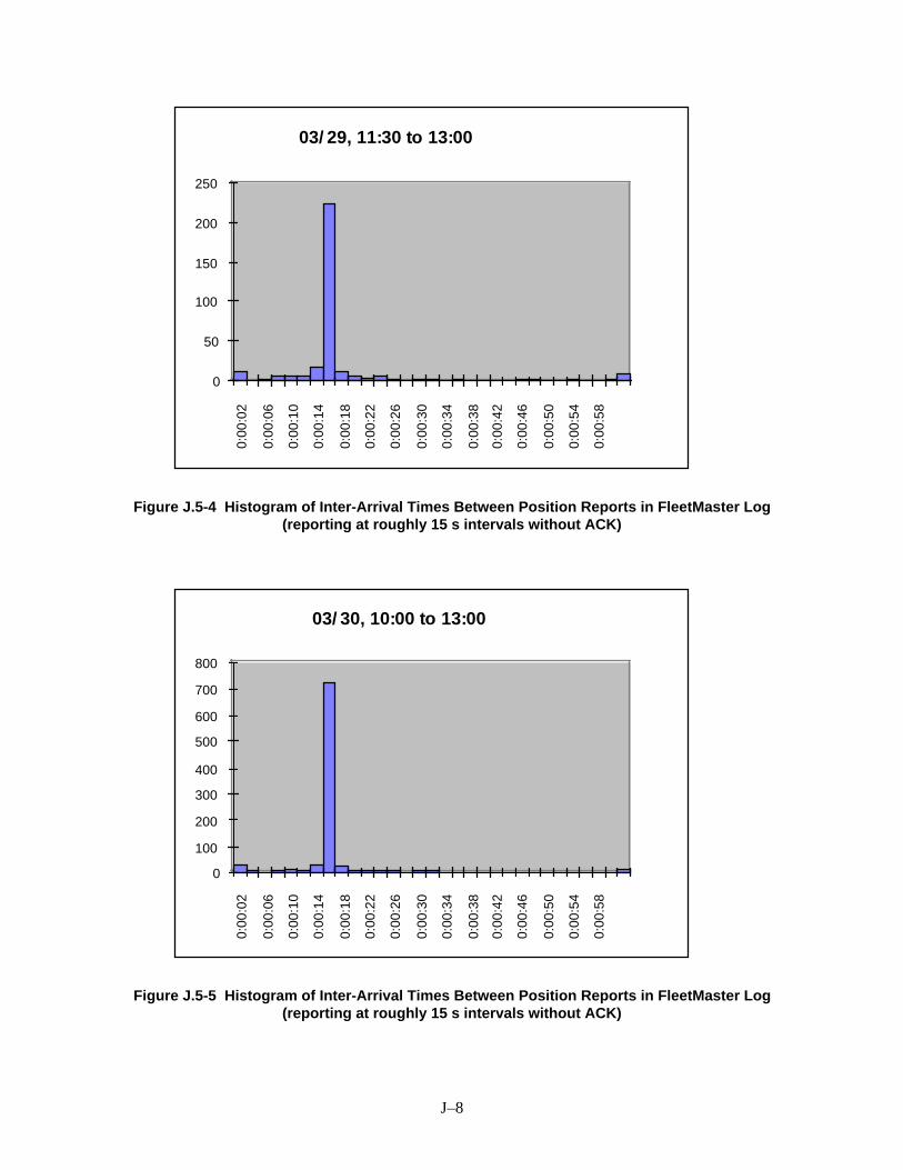
J–8
03/29, 11:30 to 13:00
0
50
100
150
200
250
0:00
:02
0:00
:06
0:00
:10
0:00
:14
0:00
:18
0:00
:22
0:00
:26
0:00
:30
0:00
:34
0:00
:38
0:00
:42
0:00
:46
0:00
:50
0:00
:54
0:00
:58
Figure J.5-4 Histogram of Inter-Arrival Times Between Position Reports in FleetMaster Log(reporting at roughly 15 s intervals without ACK)
03/30, 10:00 to 13:00
0
100
200
300
400
500
600
700
800
0:00
:02
0:00
:06
0:00
:10
0:00
:14
0:00
:18
0:00
:22
0:00
:26
0:00
:30
0:00
:34
0:00
:38
0:00
:42
0:00
:46
0:00
:50
0:00
:54
0:00
:58
Figure J.5-5 Histogram of Inter-Arrival Times Between Position Reports in FleetMaster Log(reporting at roughly 15 s intervals without ACK)

J–9
On March 30 another mobile was set to “broadcast” position reports at 15 second intervalswithout acknowledgments from the dispatch station. Only twelve out of 861 intervals exceed oneminute, indicating a success rate of 99%. This is depicted in the histogram of Figure J.5-5.
A second unit was set to “broadcast” position reports at 30 second intervals but withacknowledgments from the dispatch station. Only twenty out of 343 intervals exceed one minute,indicating a success rate of 94%.
Finally, a third unit on the same day was configured to resemble a more realistic operationalenvironment over a very wide geographic area during a three hour run. The mobile was polled bythe dispatch station at 5 minute intervals. If no response was received a second pole was sentautomatically after 30 seconds. Figure J.5-6 indicates only two instances out of thirty where theinterval between position reports differed significantly from the five minute value. This indicateda success rate of 93%.
03/30, 10:00 to 13:00
0
2
4
6
8
10
12
14
0:00
:30
0:01
:30
0:02
:30
0:03
:30
0:04
:30
0:05
:30
0:06
:30
0:07
:30
0:08
:30
0:09
:30
0:10
:30
0:11
:30
0:12
:30
0:13
:30
0:14
:30
Figure J.5-6 Histogram of Inter-Arrival Times Between Position Reports in FleetMaster Log(Polled at roughly 5 minute intervals with re-poll at 30 seconds.)
The primary conclusion to be drawn from this analysis of inter-arrival times is that coverage inthe area served by the fleet customer was generally good, with success rates ranging from 93% to99%. This includes the severe environment of downtown San Francisco. There are somelocalized areas where there are holes in CDPD coverage. These should not impact customeroperations significantly, and would be eliminated as the CDPD deployment continues.
An additional conclusion that may be drawn from the inter-arrival time data is that operation ofthe application using the UDP protocol was smooth. In general it was observed that theapplication recovered quickly from any outages which occurred due to holes in coverage. Finally,network operation seemed to be completely transparent to the application in the sense that no

J–10
significant delays are incurred in handling the CDPD traffic. As mentioned earlier, there was noperceptible variation in the performance as a function of the time of day or the voice activity onthe rest of the cellular network.
J.6 Operation in Customer’s Vehicles and Billing System Validation Tests
A billing validation test was performed using the three customer vehicles equipped withNavCells . The vehicles conducted an approximately ten hour operational run in the Bay Areaand the FleetMaster application logs were compared with information obtained from the billingsystem of GTE Mobilnet.
The NavCells of the three vehicles were configured by the FleetMaster dispatch computer totransmit at three different intervals (1) thirty seconds, (2) one minute, and (3) five minutes. Thethree vehicles had different routes. Vehicle #1 traveled from Oakland to San Francisco, spentmost of the day traveling in San Francisco, and then returned to Oakland. Vehicle #2 spent mostof the day traveling in the areas south of San Francisco, traveling from Oakland to San Francisco,to Burlingame, San Mateo, Redwood city, San Carlos, Belmont, Foster city, Hayward, SanLeandro, and then back to Oakland. Vehicle # 3 traveled primarily in the East Bay, from Oaklandto Concord, Walnut Creek, Lafayette, to San Francisco and then back to Oakland.
For the duration of this experiment, the Customer’s FleetMaster dispatch computer recorded thetransactions from the three vehicles at the specific rates (for example, thirty second intervals).The recorded transactions included the following information: (1) time, (2) status, and (3)location.
The records of the FleetMaster transactions were inspected and the total number of bytes wascalculated for each vehicle. The summary of the results is depicted in Table J.6-1, which alsopresents the reported transaction bytes from the Mobilnet billing system.
Table J.6-1. Comparison of Application Log and Billing Records
Vehicle ID Interval BetweenTransactions
Total No. of Bytes*from Customer’sFleetMaster Log
Total No. of BillableBytes from MobilnetBilling System
Deviation Between theBilling Record andCustomer FleetMaster Log
Vehicle #1 30 Sec. 82946 83376 0.5 %Vehicle #2 1 Min. 44402 44294 0.2 %Vehicle #3 5 Min. 6538 6550 0.18 %* Application (vehicle report) data payload plus the 8-byte UDP header per transaction (a few non-standard sizetransactions at power-ups are also accounted for)

J–11
J.7 Summary of Conclusions
The trial demonstrated that the CDPD network is technically very well suited to the needs offleet management systems. Specifically, it was found that:
• The CDPD system’s loading limits well exceed the requirements of the application ornetwork loading in the foreseeable future.
• End-to-end delay experienced in the CDPD network is on the order of a second and has apositive impact on operation of the application.
• Coverage in the area served by the commercial fleet customer was generally good, withtransmission success rates ranging from 93% to 99%. This included the severe environmentof downtown San Francisco. (Only a fraction of the base stations in the entire cellularterritory of GTE Mobilnet were equipped with CDPD at the time; the service roll-out hassince expanded.)
• Billing records accurately represented actual network traffic.
• CDPD modems from two manufacturers had different characteristics including differentspeed of hand-off between cells or channels.
• The UDP protocol is more suitable for operation with the FleetMaster application than TCP.In addition, UDP is more cost-efficient for the customer due to its lower packet overhead andthe elimination of transport layer ACK’s.
• A CDPD approach is a viable, cost-effective solution for fleet management operations.


![[NN40160-103] Nortel Business Communications Manager 450 1 ...€¦ · BCM450 1.0 Business Communications Manager Document Status: Standard Document Number: NN40160-103 Document Version:](https://img.dokumen.tips/doc/110x75/6027ea697a68867ff3095b86/nn40160-103-nortel-business-communications-manager-450-1-bcm450-10-business.jpg)