It’s Baaack, Twenty Years Later

Paul Krugman

February 2018

1

This paper is an exercise in self-indulgence and self-aggrandizement.

The background: In the late 1990s some U.S.-based economists began to grow disturbed about

the economic troubles facing Japan. The source of our unease wasn’t, to be honest, mainly

concern for Japan per se, or even about the impact of Japanese troubles on the global

economy. What bothered us, instead, was the sense that our intellectual framework was falling

down on the job; that Japan’s stagnation and slide into deflation called into question the

monetary policy orthodoxy of the day, which basically asserted that central bankers could

always head off deflation and get unemployment down to the NAIRU.

This unease also had a practical dimension. Japan, for all its cultural distinctiveness, is in

economic terms much like other nations, our own in particular: a big, advanced economy with

its own currency, effective administration, a competent civil service, and economic

policymakers who, if rarely ideal, aren’t usually idiots. If Japan could get stuck in an economic

trap for years on end, the same thing could happen to the rest of us.

In early 1998 I set out to reassure myself by writing down a little model to show that if Japan

was having troubles, it was simply because the Bank of Japan wasn’t trying hard enough. But as

sometimes happens when you try to model your intuitions explicitly (and is one of the main

reasons for doing formal analysis), the model ended up telling me something quite different –

namely, that when short-term interest rates are near zero it is not, in fact, easy for the central

bank to reflate the economy. In fact, even very large increases in the monetary base will have

2

essentially no effect unless the private sector is convinced that there has been a permanent

shift in the central bank’s objectives, a new willingness to accept and even promote inflation. As

I put it, the central bank needed to “credibly promise to be irresponsible.”

I wrote up that analysis in a short online theoretical paper in March 1998, then enlarged it later

that year in a Brookings paper (Krugman 1998) that took on issues of the performance of the

financial sector, the role of fiscal policy, and the relevance of historical experience.

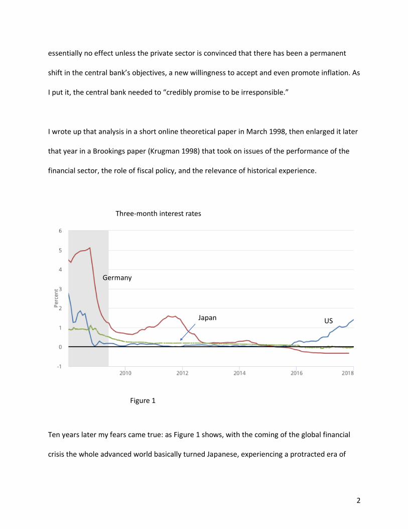
Ten years later my fears came true: as Figure 1 shows, with the coming of the global financial

crisis the whole advanced world basically turned Japanese, experiencing a protracted era of

Three-month interest rates

Germany

USJapan

Figure 1

3

near-zero interest rates. The United States has emerged from that era, barely; Europe and

Japan itself have not.

What I want to ask in this paper is how good the analytical approach of 1998 looks in the light

of subsequent experience. Were its basic predictions correct? Where did it fall down? What

new issues have arisen? And how does its policy prescription look after all these years?

1. Modeling the liquidity trap

The concept of a liquidity trap goes all the way back to Hicks (1937). Interest in the issue faded

during the long postwar boom and the inflationary, high-interest rate era that followed. Still,

some economists, notably Summers (1991), expressed concern that too low an inflation target

might lead to frequent episodes in which monetary policy was constrained by the zero lower

bound. In fact, the now-conventional 2 percent inflation target was adopted in part because

simulation analyses like Reifschneider and Williams (2000) suggested (wrongly) that 2 percent

was high enough to make ZLB episodes rare and brief.

So what was new in my 1998 analysis? Three main things, I think.

First, I framed the argument in terms of a New Keynesian model rather than some version of IS-

LM: intertemporal maximization by representative agents and rational expectations, with short-

term price stickiness the only deviation from full equilibrium. I did these things not because I

4

believe them to be an accurate description of reality – I’m very much an IS-LM fanboy – but to

give hostages, to ensure that the results weren’t being driven by the ad-hockery of Hicksian

macro.

Second, I focused on the effects of changes in the monetary base, rather than following what

had by that time become the conventional approach of modeling monetary policy in terms of

an interest rate target (e.g. as set by a Taylor rule.) Again, this was not a matter of realism, since

monetary policy at the time was in fact usually formulated in terms of interest rate targets.

Instead, it was an attempt to deal – in advance, it turned out – with an argument Bernanke

(2000) and others made, which is that expanding the money supply must, more or less as a

matter of definition, raise the equilibrium price level: “money issuance must ultimately raise

the price level, even if nominal interest rates are bounded at zero.”

This was the view I myself held before setting out to model the issue. It turned out, however,

not to be true.

Third, in the Brookings paper I spent considerable time on the implications of changes in the

monetary base on financial intermediaries and hence on broader definitions of the money

supply. This reflected contemporary policy discussions: it was common, indeed almost

conventional wisdom, to attribute Japan’s troubles to problems in its banking sector, as

evidenced by the failure of broader aggregates to expand despite supposedly loose monetary

policy. But I ended up concluding that failure of broad aggregates to rise with the monetary

5

base – a collapse of the money multiplier – is exactly what one should expect in a liquidity trap,

even if the banks are in perfectly fine shape.

I won’t rehash the theoretical model here, just summarize the key strategic simplifications. It

was, as I said, a New Keynesian-style model, but an extremely stripped-down one. There was no

explicit modeling of production, and hence no discussion of the labor market. And while the

model was infinite-horizon, I assumed that nothing would change after the second period, so

that in effect it became a two-period model, with the first period being “now” and the second

“forever after.”

The result of these simplifications was an extremely minimalist model, with an immediate,

striking implication. If, for whatever reason, the natural rate of interest in the first period was

negative – that is, it would require a negative nominal rate to achieve full employment – the

proposition that money issuance must raise the price level was false. Or if you like, it was

missing a word: permanent money issuance would raise the price level. But a monetary

expansion the private sector expected to be temporary, to be wound down after the crisis had

passed, would do nothing at all: the extra monetary base would just sit there.

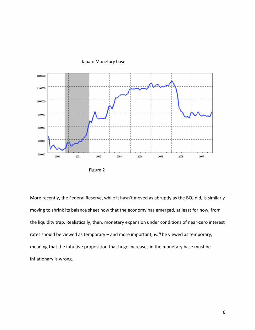
Furthermore, it was reasonable for the private sector to assume that even large increases in the

monetary base in a liquidity-trap economy would be temporary. We saw this in practice when

Japan adopted a policy of quantitative easing in the 2000s. As Figure 2 shows, this policy was

quickly reversed once the economy appeared to be recovering.

6

More recently, the Federal Reserve, while it hasn’t moved as abruptly as the BOJ did, is similarly

moving to shrink its balance sheet now that the economy has emerged, at least for now, from

the liquidity trap. Realistically, then, monetary expansion under conditions of near-zero interest

rates should be viewed as temporary – and more important, will be viewed as temporary,

meaning that the intuitive proposition that huge increases in the monetary base must be

inflationary is wrong.

Japan: Monetary base

Figure 2

7

Of course, a model is only a model, and this model didn’t even pretend to be realistic. What

matters are predictions and prescriptions: what the model says should happen, and what it

suggests about appropriate policy responses. So how has it worked out?

2. Liquidity-trap analysis in the global crisis

Although my 1998 paper focused on monetary policy, the framework had clear implications for

fiscal policy as well. In fact, I would summarize its predictions as involving two propositions

about monetary policy and two about fiscal policy. In a liquidity trap:

• Expansion of the monetary base, even if very large, would have little if any effect on

nominal GDP or the price level

• Base expansion would also have little effect on broad monetary aggregates like M2, not

because of some failure in the transmission mechanism, but because intermediaries

would have no incentive to lend out excess reserves

• Because money demand would be perfectly elastic, and there would be an incipient

excess supply of savings, there would be no crowding out: even large budget deficits

would not raise interest rates

• Because there would be no conventional crowding out, fiscal multipliers would be larger

than in normal times. In the formal model, the spending multiplier would be exactly

one; but relaxing the assumptions to allow for credit-constrained consumers would

suggest a multiplier of more than 1

8

In retrospect, these propositions may seem obvious. But they weren’t, either in 1998 or in the

midst of the post-crisis slump: many prominent figures denied one or all of them (and some still

do).

Start with the proposition that monetary expansion would be neither inflationary nor effective.

One of the discussants of that 1998 paper was Ken Rogoff, who declared that

“No one should seriously believe that the BOJ would face any significant technical problems in

inflating if it puts it mind to the matter, liquidity trap or no. For example, one can feel quite

confident that if the BOJ were to issue a 25 percent increase in the current supply and use it to

buy back 4 percent of government nominal debt, inflationary expectations would rise.”

And in 2009, Allan Meltzer declared that

“[N]o country facing enormous budget deficits, rapid growth in the money supply and the

prospect of a sustained currency devaluation as we are has ever experienced deflation. These

factors are harbingers of inflation.”

Finally, in 2010 a who’s who of conservative economists and pundits sent an open letter to Ben

Bernanke warning of dire consequences from the Fed’s policy of quantitative easing:

9

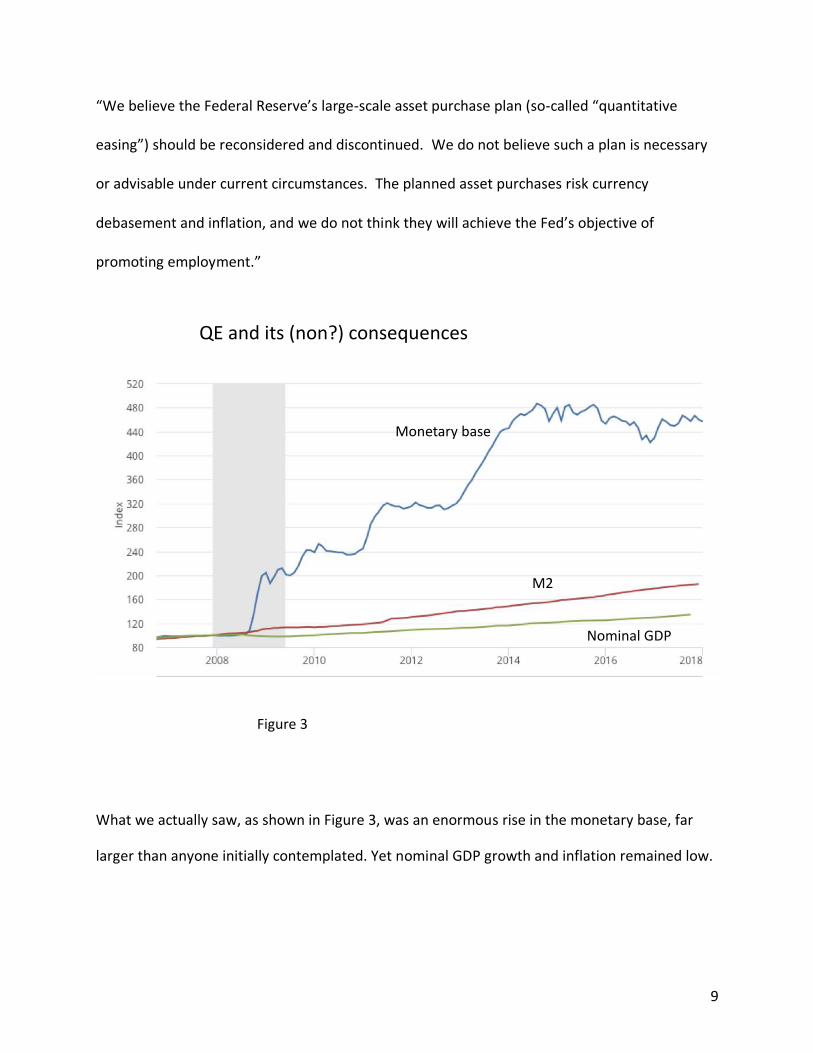
“We believe the Federal Reserve’s large-scale asset purchase plan (so-called “quantitative

easing”) should be reconsidered and discontinued. We do not believe such a plan is necessary

or advisable under current circumstances. The planned asset purchases risk currency

debasement and inflation, and we do not think they will achieve the Fed’s objective of

promoting employment.”

What we actually saw, as shown in Figure 3, was an enormous rise in the monetary base, far

larger than anyone initially contemplated. Yet nominal GDP growth and inflation remained low.

Monetary base

M2

Nominal GDP

QE and its (non?) consequences

Figure 3

10

The figure also shows strikingly little growth in M2; what growth there was probably reflected,

at least in part, a shift of funds from shadow banking, not counted in the aggregate, to insured

intermediaries.

All this was exactly as predicted, although some economists apparently didn’t get the memo.

For example, in 2013 Martin Feldstein described the failure of monetary expansion to produce

inflation as “puzzling,” and insisted that the decoupling was due to the Fed’s decision to pay

interest on excess reserves, which caused monetary base to simply accumulate in the banking

system. As it happens, the Bank of Japan did not pay such interest during the quantitative

easing episode shown in Figure 2, and saw a similar lack of results.

Deficits and interest rates

Budget balance, % of GDP

10-year

Figure 4

11

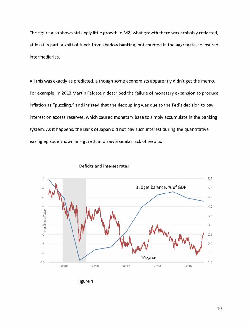
What about deficits and interest rates? As Figure 4 shows, huge U.S. deficits in 2009-12 were

actually associated with interest rates that were low by historical standards, as liquidity-trap

analyses predicted. This was very much not what many influential figures, including some

economists, expected to happen. The Wall Street Journal seized on an uptick in long-term rates

in early 2009 to publish an editorial titled “The bond vigilantes: The disciplinarians of U.S. policy

makers return.” In 2010 Alan Greenspan, writing in the Financial Times, came out with one of

my favorite economic pronouncements of all time (emphasis mine):

“Despite the surge in federal debt to the public during the past 18 months—to $8.6 trillion from

$5.5 trillion—inflation and long-term interest rates, the typical symptoms of fiscal excess, have

remained remarkably subdued. This is regrettable, because it is fostering a sense of

complacency that can have dire consequences.”

Some historians of science tell us that the conventional view of how theories get accepted –

that they are tested against evidence, and accepted if they pass – isn’t quite right. What

matters is that a theory make surprising predictions, ones that run counter to conventional

wisdom, and is proved right.

That seems to me to be a pretty good description of how liquidity-trap economics fared in the

aftermath of the financial crisis. The theory made predictions about inflation, monetary

aggregates, and interest rates that were very much at odds with what many people believed;

those predictions were proved correct.

12

So far, however, I haven’t gotten to the fourth prediction, large fiscal multipliers. That’s

because there’s more controversy about what the evidence says. Clearly we didn’t have

runaway inflation or soaring interest rates. But evaluating the effect of fiscal policy takes a bit

more parsing of the data. Skeptics of the liquidity-trap case, I’d argue, have misunderstood how

to frame the issue. But let me take a moment first to point out that here, too, many influential

voices, both among academic economists and among policymakers, vehemently disagreed with

the proposition that fiscal multipliers would be large, or even positive.

Why? There were actually three distinct anti-Keynesian arguments, in each case made by

people one would not normally have regarded as cranks.

First, one set of economists essentially resurrected Say’s Law: they insisted that since income

must be spent, any increase in public spending must, by definition, crowd out an equal amount

of private spending. (See the discussion in Krugman 2009.)

Second, another set of economists managed to convince themselves, wrongly, that Ricardian

equivalence implies a zero multiplier on government spending. (See Krugman 2011.) Actually,

my original paper laid out a model with full Ricardian equivalence, in which the multiplier on

short-term increases in government spending was 1.

13

Most consequentially for actual policy, many policymakers were persuaded by the arguments

of Alesina and Ardagna (2010) that spending cuts would actually be expansionary, because they

would improve confidence. Here’s Jean-Claude Trichet in 2010:

“As regards the economy, the idea that austerity measures could trigger stagnation is incorrect

… In fact, in these circumstances, everything that helps to increase the confidence of

households, firms and investors in the sustainability of public finances is good for the

consolidation of growth and job creation. I firmly believe that in the current circumstances

confidence-inspiring policies will foster and not hamper economic recovery, because

confidence is the key factor today.”

Now, empirical analysis of fiscal policy is notoriously difficult, because of the endogeneity of

both revenues and, to a lesser extent, spending. The raw correlation between budget deficits

and output is negative, but everyone understands that this is because recessions cause

revenues to shrink and spending on safety-net programs to grow.

Yet simply attempting to purge the cyclical component of the deficit, as Alesina and Ardagna

did, is problematic. For one thing, statistical techniques for doing so don’t seem to work very

well: it was immediately obvious to many readers of the A-A work that their episodes of fiscal

expansion and contraction didn’t seem to correspond to known policy changes; an IMF analysis

that used narrative evidence on actual policy reversed their main result. Even identifying the

policy right, however, doesn’t deal with the problem that stimulus programs are likely to be

14

implemented when the economy is weak (as in the case of the Obama stimulus) and austerity

programs often implemented, or at least delayed until, the economy is strong.

There are a variety of ways one might try to circumvent these problems, but as it happens the

crisis itself provided something approximating a natural experiment: the debt panic that

followed the 2009 Greek crisis. Following that crisis, some countries either chose or were

forced into severe fiscal austerity despite high unemployment and the inability to pursue

offsetting monetary expansion. Others were under less pressure.

This wasn’t a perfect natural experiment, because arguably some of the countries forced into

the harshest austerity were troubled in other ways. Still, as Blanchard and Leigh (2013) pointed

out, one can at least partially deal with this issue by comparing economic performance with

forecasts generated before austerity went into effect.

It’s important to note, by the way, that this natural experiment took place over a limited period

– 2009 to 2012 or 2013. Why? Because that’s how long the debt panic lasted. Once Mario

Draghi issued his famous pronouncement that the ECB would do “whatever it takes,” bond

spreads rapidly dropped and the pressure on governments to engage in extreme austerity

policies faded. As a result, all the usual measurement and endogeneity issues apply to data

from subsequent years.

15

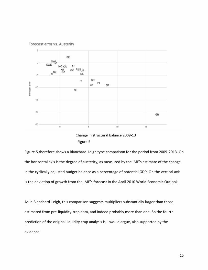
Figure 5 therefore shows a Blanchard-Leigh type comparison for the period from 2009-2013. On

the horizontal axis is the degree of austerity, as measured by the IMF’s estimate of the change

in the cyclically adjusted budget balance as a percentage of potential GDP. On the vertical axis

is the deviation of growth from the IMF’s forecast in the April 2010 World Economic Outlook.

As in Blanchard-Leigh, this comparison suggests multipliers substantially larger than those

estimated from pre-liquidity-trap data, and indeed probably more than one. So the fourth

prediction of the original liquidity-trap analysis is, I would argue, also supported by the

evidence.

Change in structural balance 2009-13

Figure 5

16

Overall, this is a pretty good record! An analysis made a decade before the global financial

crisis, based on theory with a bit of historical evidence from the 1930s, ended up providing a

good guide to monetary and fiscal policy post-2008 – a much better guide than the views held

by many influential policymakers.

3. Can monetary policy be effective in a liquidity trap?

In 1998 I argued that while a monetary expansion perceived as temporary would be ineffective

in a liquidity trap, an expansion perceived as permanent would work – because it would raise

the expected rate of inflation, and hence reduce real interest rates. So I declared that the Bank

of Japan needed to “credibly promise to be irresponsible,” making clear its willingness to

tolerate higher inflation.

A more diplomatic way to put this prescription, and the way many economists now do put it, is

to say that when nominal rates are near zero, gaining monetary traction requires convincing

markets that there has been a monetary regime change. So what have we learned about the

usefulness of this prescription since 2008?

The first thing we’ve learned, disappointingly, is how hard it is to get central bankers to

consider a regime change.

17

Since the 1990s there has been a wide consensus that responsible monetary policy, with a due

concern for price stability, means having an inflation target of 2 percent. Why 2, as opposed to

1 or 3? Well, that’s a funny story. Partly it’s New Zealand’s fault: as the first central bank to

explicitly adopt an inflation target, their choice has had an effect utterly disproportionate to

their economic weight or population (even if you include the sheep.)

But 2 percent also seemed to be a good compromise among different factions in the economic

policy community. Those who believed that “price stability” should mean zero inflation were

willing to accept 2 percent on the grounds that given unmeasured gains from technological

progress, 2 might really be zero. Meanwhile, as mentioned before, those who worried about

hitting the zero lower bound believed that 2 was high enough to largely eliminate that concern.

And 2 percent inflation also seemed high enough to eliminate most problems associated with

downward nominal wage rigidity.

We now know, however, that the assumptions underlying the 2 percent solution were all

wrong. Despite a 2 percent inflation target, the U.S. spent 7 years at the zero lower bound, and

the euro area is still there. Downward nominal wage rigidity turned out to be a significant issue

in the United States, and a huge issue in southern Europe, where it greatly increased the

difficulty of achieving internal devaluation in Spain and especially Portugal.

Given the way experience has undermined much of the original case for a 2 percent inflation

target, and given the severity of the economic crisis, you might therefore have expected some

18

revision – a rise in the inflation target, or a shift to some other kind of targeting – price level or

nominal GDP targeting. But that hasn’t happened. Even though a 2 percent inflation target is an

essentially arbitrary number, it has become a focal point, a sort of token of respectability that

almost no central bankers are willing to meddle with. (In this sense it resembles the role once

played by the gold standard.)

This is quite remarkable. If the worst economic crisis since the 1930s, one that cumulatively

cost advanced nations something on the order of 20 percent of GDP in foregone output, wasn’t

enough to provoke a monetary regime change, it’s hard to imagine what will.

This in turn might seem to suggest that while monetary policy could in principle offer a solution

to the problem of the zero lower bound, fiscal policy ends up being the only realistic tool.

Unfortunately, fiscal responses were pretty bad too: a brief, modest turn toward stimulus at

the beginning of the crisis was followed by austerity in the midst of high unemployment and

impotent monetary policy.

Aside from the economic and human costs of this failure to act, the unwillingness and/or

inability of central bankers to even attempt regime change means that we don’t have much

evidence on whether the monetary policy prescriptions from liquidity-trap analysis could work

in practice. There is, however, one exception: the place where it all began, Japan.

19

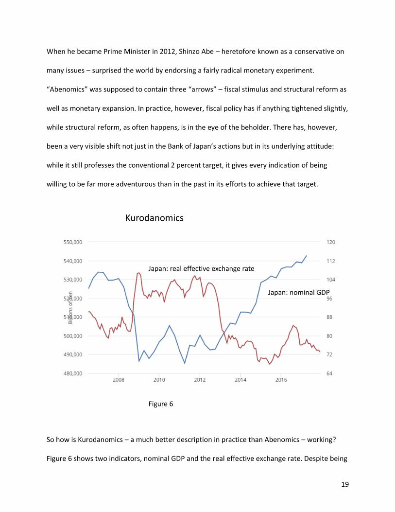
When he became Prime Minister in 2012, Shinzo Abe – heretofore known as a conservative on

many issues – surprised the world by endorsing a fairly radical monetary experiment.

“Abenomics” was supposed to contain three “arrows” – fiscal stimulus and structural reform as

well as monetary expansion. In practice, however, fiscal policy has if anything tightened slightly,

while structural reform, as often happens, is in the eye of the beholder. There has, however,

been a very visible shift not just in the Bank of Japan’s actions but in its underlying attitude:

while it still professes the conventional 2 percent target, it gives every indication of being

willing to be far more adventurous than in the past in its efforts to achieve that target.

So how is Kurodanomics – a much better description in practice than Abenomics – working?

Figure 6 shows two indicators, nominal GDP and the real effective exchange rate. Despite being

Japan: real effective exchange rate

Japan: nominal GDP

Kurodanomics

Figure 6

20

at (or slightly below) the zero lower bound, the Bank of Japan evidently managed to achieve

considerable traction. It has not so far managed to achieve the inflation target, but at least the

Japanese experiment suggests some support for the view that monetary regime change can be

effective even at the zero lower bound. Credibly promising to be irresponsible makes a

difference; the problem is that central bankers won’t do it.

Before pronouncing Kurodanomics a vindication of the 1998 view, however, I would raise a

question that worries me both about Japan and about the role of monetary policy in general:

what happens to the analysis if we really do face a future of secular stagnation?

Since there still seems to be a lot of confusion – willful confusion? – about what secular

stagnation means, let’s be clear: it has nothing to do with the economy’s growth rate, certainly

not in the short run and maybe not even in the long run. Instead, it’s the proposition that for

whatever reason the natural rate of interest, the interest rate consistent with full employment,

will on average be negative for a long time. This in turn means that liquidity-trap conditions will

become the norm, not the exception – rather than an economy that goes through brief

episodes at the zero lower bound in the aftermath of exceptional busts, we will have an

economy in which the ZLB is binding most of the time, except during exceptional

booms/bubbles.

This was not the way I modeled the liquidity trap in 1998, or how Eggertsson and Woodford

modeled it in 2003. In these papers the assumption was that after a period of depressed

21

demand, the economy would return to a regime with a positive natural rate of interest. Once

the economy returned to “normal”, conventional monetary policy would regain traction. So

what the central bank needed to do was commit to a higher price level in this future period

when it would have regained its normal superpowers.

But if a negative natural interest rate is the new normal, how can the central bank gain

traction? The answer seems to be that it must create a self-fulfilling prophecy of higher

inflation: it must convince the market that it will achieve inflation; this higher expected inflation

reduces real interest rates; and lower real interest rates create an economic boom that

generates the expected inflation.

This is obviously even harder than convincing the market that there has been a monetary

regime change. And it also raises the prospect of what I’ve called the timidity trap: if the

inflation target is set too low, it won’t generate the required economic boom even if markets

believe the central bank will hit it. I find this especially worrisome for Japan, where

demographic factors – a rapidly shrinking working-age population – suggest that the

conventional 2 percent target might well be too low to achieve economic escape velocity.

But let me not end on a down note. I began this paper by framing it as an assessment of how

modern liquidity-trap analysis, brought into being two decades ago in an attempt to make

sense of Japan’s problems, has fared in the aftermath of a global crisis that produced Japan-like

conditions in many countries. And the answer, I’d argue, is that it has done very well.

22

Put it this way: If economists were like natural scientists, we’d be celebrating the success of our

standard model. Confronted with conditions very different from those encountered in the past,

the model made predictions very much at odds with the expectations of many policymakers

and market participants. And those predictions proved correct.

Now, it’s true that policymakers by and large ignored this successful analysis, with ugly results

for the real world. It’s also true that essentially nobody who was wrong has admitted error, or

changed his views. But aside from that, this is basically a happy story.

REFERENCES

Alesina, A. and Ardagna, S. (2010), “Large changes in fiscal policy: taxes versus spending” in J.

Brown, ed., Taxes and the Economy.

Bernanke, B. (2000), “Japanese Monetary Policy: A Case of Self-Induced Paralysis?” in Japan’s

Financial Crisis and Its Parallels to U.S. Experience, Ryoichi Mikitani and Adam Posen, eds.,

Institute for International Economics.

Blanchard, O. and Leigh, D. (2013), “Growth forecast errors and fiscal multipliers,”, American

Economic Review

Eggertsson, G. and Woodford, M. (2003), “The zero bound on interest rates and optimal monetary policy,” Brookings Papers on Economic Activity, 1. Hicks, J. (1937), “Mr. Keynes and the classics,” Econometrica.

Krugman, P. (1998), “It’s baaack: Japan’s slump and the return of the liquidity trap,” Brookings

Papers on Economic Activity, 2, 137-187.

Krugman, P. (2009), “A dark age of macroeconomics,” at

https://krugman.blogs.nytimes.com/2009/01/27/a-dark-age-of-macroeconomics-wonkish/

23

Krugman, P. (2011), “Ricardian confusions”, at

https://krugman.blogs.nytimes.com/2011/03/10/ricardian-confusions-wonkish/

Reifschneider, David L., and John C. Williams. (2000) “Three Lessons for Monetary Policy in a

Low-Inflation Era.” Journal of Money, Credit and Banking, 32:4-2, 936-66.

Summers, L. (1991), “Panel Discussion: Price Stability, How Should Long-Term Monetary

Policy Be Determined?”, Journal of Money, Credit and Banking 23(3), pp. 625-631.