Iterative factorization of the error system in

Moment Matching and applications to error bounds

Heiko Panzer, Thomas Wolf, Boris Lohmann

GAMM-Workshop – Applied and Numerical Linear AlgebraBremen, 22.09.2011

Heiko Panzer 2

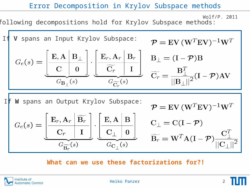
Error Decomposition in Krylov Subspace methods

If V spans an Input Krylov Subspace:

If W spans an Output Krylov Subspace:

Wolf/P. 2011The following decompositions hold for Krylov Subspace methods:

What can we use these factorizations for?!

Heiko Panzer 3

Feature 1: Numerical advantage

Compare the classical error system…

…to its new formulation…

contains twice the (almost) same dynamics

subtraction is performed in the output signals

small scale and easy to analyze

invariant zeros at expansion points,poles equal to those of Gr(s)→ all-pass for IRKA/ISRK

very similar to G(s)input vector/matrix contains subtraction

Heiko Panzer 4

Numerical advantage II

Example: Reduce ISS model [2] using RK-ICOP [Eid 2009]

q = 14ICOP: sopt = 0.94

Assume we want to perform a second reduction step starting from G(s)-Gr(s)

q = 14ICOP: sopt = 0.77

Use GB┴ instead:

ICOP: sopt = 37.7 → Detected frequency much better suited

Heiko Panzer 5

Numerical advantage III

Example: ISS model

→ Additional information is available and can be used to optimize RK-ICOP!

Heiko Panzer 6

Feature 2: H2-error in SVD-Krylov-methods

The Gramian Q is assumed to be known anyway in SVD-Krylov.→ Cheap error bound!

Special case ISRK [4]:

All-pass in case oflocally H2-optimal reduction

small scale

Wolf/P. 2011

Heiko Panzer 7

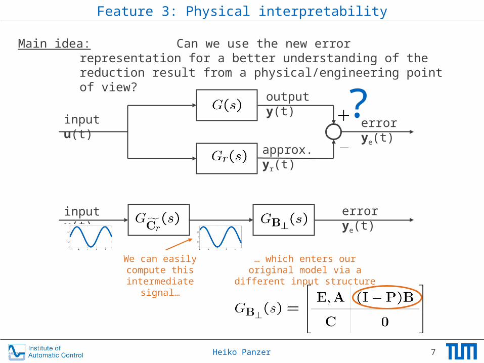
Feature 3: Physical interpretability

Main idea: Can we use the new error representation for a better understanding of the reduction result from a physical/engineering point of view?

input u(t) error ye(t)

input u(t) error ye(t)

approx. yr(t)

output y(t) ?

We can easily compute this intermediate signal…

… which enters our original model via a different input structure

Heiko Panzer 8

Physical interpretability II

input u(t) error ye(t)

Example: Continuous heat equation [2] Rational Krylov. n=200, q=15

not all-pass, but amplitude is diminished

at all frequencies

→ The error resulting from MOR is equivalent to the output caused by a minor additional heat source. An engineer might regard this as admissable.

Heiko Panzer 9

Feature 4: Iterative decomposition

qq2 nq q2

qq2 nq q2q

qq2q q2q q3 n q3

qq2q q2q q3 n q3qq2

∑qi n ∑qi

Let V form an Input Krylov Subspace

2nd reduction

3rd reduction

Heiko Panzer 10

Iterative decomposition II

q q2 nq q2

qq2 nq q2q

qq2q q2q q3 nq3

qq q2q3 nq3q q2

∑qi n∑qi

q q2

Let W form an Output Krylov Subspace

2nd reduction

3rd reduction

Heiko Panzer 11

Iterative decomposition III

qq2q q2q q3 nq3qq2

∑qi n ∑qiV

One can iteratively influence the input and output matrices of the remaining large scale model according to one‘s objectives!

∑qiW

from Output Krylovdecomposition

from Input Krylov decomposition

large scale

Heiko Panzer 12

Feature 5: Dissipativity-based error bound

A large class of systems fulfills

→ Positive definite E

→ Strictly dissipative A

This is e.g. true for port-Hamiltonian systems with R > 0 or can be achieved for typical second order systems.

Then:

compute iteratively(inexpensive!)

P./Wolf ACC2012

Heiko Panzer 13

Dissipativity-based error bound II

use bound for dissipative systems

easy to compute

Objectives:

• Iteratively lower bound on G*(s) by making B┴ and C┴ smaller

→ orthogonal projection with W=V

• Keep feedthrough-filters close to all-pass (avoid peaks that boost H∞-norm)→ IRKA/ISRK or pole-placement algorithms

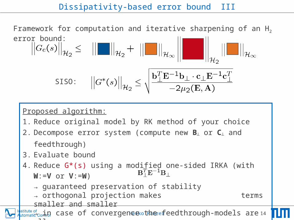
Framework for computation and iterative sharpening of an H2 error bound:

goal conflict

Heiko Panzer 14

Dissipativity-based error bound III

Proposed algorithm:

1. Reduce original model by RK method of your choice

2. Decompose error system (compute new B┴ or C┴ and feedthrough)

3. Evaluate bound

4. Reduce G*(s) using a modified one-sided IRKA (with W:=V or V:=W)

→ guaranteed preservation of stability→ orthogonal projection makes terms smaller and smaller→ in case of convergence the feedthrough-models are all-pass

5. Return to step 2.

Framework for computation and iterative sharpening of an H2 error bound:

SISO:

Heiko Panzer 15

Feature 5: Dissipativity-based error bound

Example: CD Player [2]

Heiko Panzer 16

Feature 5: Dissipativity-based error bound

Example: Butterfly Gyroscope [2]

Heiko Panzer 17

Conclusions

The new factorization…

• is most inexpensive to compute

• exhibits nice numerical behaviour

• offers cheap H2 error expressions in SVD-Krylov-methods like ISRK

• makes the error physically interpretable

• can be iteratively applied

• provides a purely Krylov-based H2 error bound for strictly dissipative systems

But…

• we need a strategy how the iterative reductions must be performed

• we have no experience with MIMO, so far

Heiko Panzer 18

Bibliography

[1] R. Eid: Time Domain Moment Matching. PhD Thesis. TU München, 2009.

[2] Oberwolfach Model Reduction Benchmark Collection.Available online at http://www.imtek.uni-freiburg.de/simulation/benchmark/

[3] H. Panzer, J. Hubele, R. Eid and B. Lohmann: Generating a Parametric Finite Element Model of a 3D Cantilever Timoshenko Beam Using Matlab. TRAC-4 Number 3. 2009. Available online at www.rt.mw.tum.de

[4] S. Gugercin, An iterative SVD-Krylov based method for model reduction of large-scale dynamical systems. Linear Algebra and its Applications, 2008.