Embed Size (px)
Citation preview

MAU130010 Rev D
MicroCal, LLC 22 Industrial Drive East
Northampton, MA 01060 USA Phone: +413 586 7720
Fax: +413 586 0149 Binding Stability Kinetics [email protected]
ITC Data Analysis in Origin®
Tutorial Guide Version 7.0 - January 2004
Using Origin® scientific plotting software to analyze calorimetric data from all
MicroCal Isothermal Titration Calorimeters

Table of Contents
MAU130010 Rev D
Table of Contents Introduction to ITC Data Analysis...............................................................................1 Getting Started...............................................................................................................3
System Requirements...................................................................................................................3 Installing Origin - Single User License........................................................................................3 Installing Origin for ITC Custom Disk ........................................................................................3 Registering with OriginLab..........................................................................................................4 Starting Origin..............................................................................................................................5 Menu Levels.................................................................................................................................5 Simultaneously Running DSC, ITC and PPC Configurations .....................................................6 View Mode...................................................................................................................................6 A Note About Data Import...........................................................................................................7 Opening and Analyzing Previous Versions of Origin (*.ORG) Documents ................................7
Lesson 1: Routine ITC Data Analysis and Fitting ......................................................9 Routine ITC Data Analysis ..........................................................................................................9 Curve Fitting ................................................................................................................................13 Fitting Parameter Constraints.......................................................................................................14 Fitting Parameters Text ................................................................................................................14 Creating a Final Figure for Publication........................................................................................17
Lesson 2: Setting Baseline and Integration Range.....................................................21 Lesson 3: Deleting Bad Data ........................................................................................27 Lesson 4: Analyzing Multiple Runs and Subtracting Reference..............................29
Opening Multiple Data Files ........................................................................................................29 Adjusting the Molar Ratio............................................................................................................33 Subtracting Reference Data..........................................................................................................34 Subtracting Reference Data: Additional Topics..........................................................................36
Lesson 5: ITC Data Handling ......................................................................................43 Reading Worksheet Values from Plotted Data.............................................................................43 Copy and Paste Worksheet Data ..................................................................................................45 Exporting Worksheet Data ...........................................................................................................46 Importing Worksheet Data ...........................................................................................................48
Lesson 6: Modifying Templates...................................................................................49 Modifying the DeltaH Template ..................................................................................................49 Modifying the RawITC template .................................................................................................52 A Note About Units .....................................................................................................................53
Lesson 7: Advanced Curve Fitting ..............................................................................55 Fitting with the Two Sets of Sites Model.....................................................................................55 NonLinear Least Squares Curve: Fitting Session........................................................................58 Controlling the Fitting Procedure.................................................................................................59 Deconvolution with Ligand in the Cell and Macromolecule in the Syringe ................................60 Deconvolution with the Sequential Binding Sites Model ............................................................63 Enzyme/substrate/inhibitor Assay................................................................................................66 Dimer Dissociation Model ...........................................................................................................75 Competitive Ligand Binding........................................................................................................77 Simulating Curves........................................................................................................................79 Using Macromolecule Concentration, rather than n, as a Fitting Parameter ................................82 Single Injection Method...............................................................................................................82

MAU130010 Rev D
Lesson 8: Autosampler Data (Optional Accessory) ...................................................89
Launching the ITC Autosampler Data Session ............................................................................89 Auto ITC Buttons.........................................................................................................................91 Single Injection Method with AutoITC........................................................................................95
Lesson 9: Other Useful Details ....................................................................................101 Chi-square (chi^2) Minimization .................................................................................................101 Line Types for Fit Curves ............................................................................................................101 Inserting an Origin graph into Microsoft® Word .........................................................................102 Calculating a Mean Value for Reference Data.............................................................................103
Appendix: Equations Used for Fitting ITC Data.......................................................105 I. General Considerations............................................................................................................105 II. Single Set of Identical Sites....................................................................................................106 III. Two Sets of Independent Sites ..............................................................................................107 IV. Sequential Binding Sites .......................................................................................................108 V. Enzyme/substrate/inhibitor Assay ..........................................................................................110 VI. Dimer Dissociation Model ....................................................................................................111 VII. Competitive Binding Model ................................................................................................112 VIII. Single Injection Method .....................................................................................................113
Index................................................................................................................................115

Getting Started
MAU130010 Rev D 1
Introduction to ITC Data Analysis
Origin is a general purpose, scientific and technical data analysis and plotting tool. In addition, Origin can carry add-on routines to solve specific problems. Analyzing isothermal titration calorimetric (i.e., ITC) data from the OMEGA, MCS or VP-ITC instruments is one such specific application. This version of Origin includes routines designed to analyze ITC data. Most of the ITC routines are implemented as buttons in plot window templates designed specifically for the ITC data analysis software. Some routines are located in the ITC menu in the Origin menu display bar. This tutorial will show you how to use all of the ITC routines. Lesson 1 provides an overview of the ITC data analysis and fitting process, and should be read first. The subsequent lessons each look in more detail at particular aspects of ITC data analysis, and may be read in whatever order you see fit. If you are unfamiliar with the basic operation of Origin, you may find it helpful to read through OriginLab's Origin - Getting Started Manual (particularly the introductory chapter). Note that this ITC tutorial contains information about Origin only in so far as it applies to ITC data analysis. If you have questions or comments, we would like to hear from you. Technical support and customer service can be reached at the following numbers: Toll-Free in North America: 800.633.3115 Telephone: 413.586.7720 Fax: 413.586.0149 Email: [email protected] Web Page: www.microcalorimetry.com

ITC Tutorial Guide
2 MAU130010 Rev D
This page was intentionally left blank

Getting Started
MAU130010 Rev D 3
Getting Started In this chapter we describe how to install Origin on your hard drive, how to configure Origin to include the ITC add-on routines, and how to start Origin.
System Requirements
Origin version 7 requires the following minimum system configuration: • Microsoft Windows® 95 or later or Windows NT® version 4.0 or later. • 133 MHz or higher Pentium compatible CPU. • 64 megabytes (MB) of RAM • CD-ROM drive. • 50 MB of free hard disk space. • Internet Explorer version 4.0 or later (we recommend version 5.0 or later). Internet
Explorer need not be your default browser, but it must be installed for viewing Origin's compiled HTML Help.
Installing Origin - Single User License
Note: We recommend that when installing Origin you do not accept the default directory, but choose the folder C:\Origin70\
To install a new copy of Origin or to upgrade an existing copy, insert the Origin 7 CD into your CD-ROM. A window opens with a number of options, including installing Origin. Click the link to install Origin. If the CD does not start automatically, browse the CD and run ORIGINCD.EXE directly. The Setup program prompts you to type in your Origin serial number and license key. These numbers are located inside your registration card in the Origin product package.
Please refer to the 'Origin : Getting Started Booklet' for further information (When choosing a Destination directory (or folder) name to place Origin, make sure this name or any other name in the path does not include a space, otherwise Origin will not operate properly).
After installation is complete you will see the Origin70 program folder with the program icons. If you wish to create a shortcut desktop icon you may do the following. Right click the MicroCal LLC ITC icon and select copy from the drop down menu, then right click anywhere on the desktop and select paste to install a desktop icon for Origin ITC.
Installing Origin for ITC Custom Disk
After installing Origin you will need to install the Custom disk for the ITC routines (if you have purchased other options, the relevant Autosampler, PPC and DSC routines will be included on this disk).
• Insert the Custom Disk CD into your CD-ROM

ITC Tutorial Guide
4 MAU130010 Rev D
• Using Windows Explorer, navigate to the AddOn Setup sub folder of the Origin 7.0
folder, and open the Setup.exe application file by double clicking on the filename.
Note: you may also launch the setup up program by selecting Run from the Start Menus then entering c:\Origin70\AddOn Setup\Setup.exe into the text box and clicking OK.
• Follow the instructions on screen.
Registering with OriginLab
Select the AddOn Setup Folder
Double click on Setup.exe file

Getting Started
MAU130010 Rev D 5
OriginLab™ Corporation., a separate company from MicroCal™ , LLC., produces and supports the Origin software package. MicroCal™, LLC. produces and supports the calorimetric fitting routines imbedded in the Origin for DSC and Origin for ITC packages. MicroCal, LLC. will provide technical support for all aspects of the software without registration. OriginLab Corp. will not provide technical support for the calorimetric fitting routines, but if the copy is registered, will provide standard technical support for the general purpose routines of the program . Upon receipt of Origin, please fill out and return the registration form included with your package to OriginLab. You may also register at any time by contacting the Customer Support Department at OriginLab.
Starting Origin
To start Origin, double-click on the Origin 7.0 program icon on the Desk Top. Alternatively, click Start, then point to Programs then point to the OriginLab folder then click on the MicroCal LLC ITC program icon from the submenu.
Menu Levels
This ITC version of Origin comes with a minimum of three distinct menu configuration options, or menu levels (there are other levels available if you purchased the optional DSC, PPC, or Autosampler DSC software ). Each menu level has its own distinct menu commands. After Origin has opened you may change a menu level option under the Format : Menu option. The nine menu levels are: General Full Menus - Select this option to run Origin in the generic, non-instrument mode. This menu level contains no instrument-specific routines, but does contain many general data analysis and graphics routines, not present in the instrument-specific menus, that you may find useful for other applications. ITC Data Analysis - Select this option to run Origin in a configuration that includes the instrument-specific ITC data analysis routines. Single Injection ITC Data Analysis - Select this option to run Origin in a configuration that analyzes Single Injection ITC experiments. Autosampler ITC Data Analysis - Select this option to run Origin in a configuration that includes the instrument specific autosampler with ITC data analysis routines for handling multiple data files. Note that this menu level is available only if you purchased the optional AutoITC software module. AutoITC Single Injection Data Analysis - Select this option to run Origin in a configuration that analyzes multiple data files of Single Injection ITC experiments. Note that this menu option is available only if you purchased the AutoITC software module. DSC Data Analysis - Select this option to run Origin in a configuration that includes the instrument-specific DSC data analysis routines. Autosampler DSC Data Analysis - Select this option to run Origin in a configuration that includes the instrument specific autosampler with DSC data analysis routines for

ITC Tutorial Guide
6 MAU130010 Rev D
handling multiple data files. Note that this menu level is available only if you purchased the autosampler DSC software module. PPC Data Analysis - Select this option to run Origin in a configuration that includes the instrument-specific PPC data analysis routines. Note that this menu level is available only if you purchased the optional DSC with the PPC attachment. Short Menus - Select this option to run Origin with menus that are an abbreviated version of the General Full Menus configuration. Note that you cannot switch to a new menu level if there is a maximized plot window or worksheet in the current project. A warning prompt will appear if you try to switch levels while a window is maximized. If this happens, simply click on the window
Restore button. You will then be able to switch levels.
Simultaneously Running DSC, ITC and PPC Configurations
If you purchased the DSC, ITC, Autosampler and PPC software modules, the installation program will have automatically created icons in the MicroCal OriginLab program group for the relevant software. This allows you to run the configurations simultaneously. The most likely reason to do this would be if you have the MicroCal DSC with the PPC or Autosampler attachment and the MicroCal ITC microcalorimeters, and you intend to run them on the same computer. Double-click on any icon to run that configuration.
View Mode
Each Origin plot window can be viewed in any of four different view modes: Print View, Page View, Window View, and Draft View. These are available under the View menu option. Print View is a true WYSIWYG (What You See is What You Get) view mode. This view mode displays a page that corresponds exactly to the page from your hard copy device. Exact font placement and size is guaranteed, at some sacrifice to screen appearance, since the printer driver fonts must be scaled to fit their positions on the page (this will not harm the appearance of true vector fonts). This is a slow process, and screen refresh speed suffers as a result. Thus, reserve the Print View mode for previewing your work prior to printing. Origin automatically changes to Print View mode when graphics are exported to another application and when printing. The view mode automatically returns to the selected view mode after the operation is complete. Page View provides faster screen updating than Print View , but does not guarantee exact text placement on the screen unless you are using typeface scaling software (such as Adobe Type Manager). Use Page View mode until your application is ready for printing or copying to another application. Change to Print View mode to check object placement before exporting, copying, or printing.
Getting Started
MAU130010 Rev D 7
Window View expands the page to fill up the entire graph window. Labels, buttons, or other objects in a graph window that reside in the gray area of the page are not visible in Window View mode. Draft View has the fastest screen update of the four view modes. In Draft View, the page automatically sizes to fill the graph window. This is a convenient mode to use when you are primarily interested in looking at on-screen data. Note that view mode will not affect your print-outs. Only on-screen display is affected.
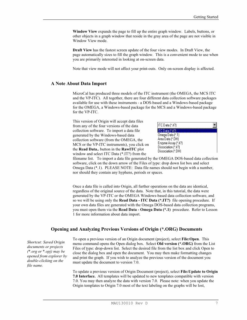
A Note About Data Import
MicroCal has produced three models of the ITC instrument (the OMEGA, the MCS ITC and the VP-ITC). All together, there are four different data collection software packages available for use with these instruments - a DOS-based and a Windows-based package for the OMEGA, a Windows-based package for the MCS and a Windows-based package for the VP-ITC. This version of Origin will accept data files from any of the four versions of the data collection software. To import a data file generated by the Windows-based data collection software (from the OMEGA, the MCS or the VP-ITC instruments), you click on the Read Data.. button in the RawITC plot window and select ITC Data (*.IT?) from the filename list. To import a data file generated by the OMEGA DOS-based data collection software, click on the down arrow of the Files of type: drop down list box and select Omega Data (*.1). PLEASE NOTE: Data file names should not begin with a number, nor should they contain any hyphens, periods or spaces. Once a data file is called into Origin, all further operations on the data are identical, regardless of the original source of the data. Note that, in this tutorial, the data were generated by the VP-ITC or the OMEGA Windows-based data collection software, and so we will be using only the Read Data - ITC Data (*.IT?) file opening procedure. If your own data files are generated with the Omega DOS-based data collection programs, you must open them via the Read Data - Omega Data (*.1) procedure. Refer to Lesson 1 for more information about data import.
Opening and Analyzing Previous Versions of Origin (*.ORG) Documents
To open a previous version of an Origin document (project), select File:Open. This menu command opens the Open dialog box. Select Old version (*.ORG) from the List Files of type: drop-down list. Select the desired file from the list box and click Open to close the dialog box and open the document. You may then make formatting changes and print the graph. If you wish to analyze the previous version of the document you must update the document to version 7.0. To update a previous version of Origin Document (project), select File:Update to Origin 7.0 Interface. All templates will be updated to new templates compatible with version 7.0. You may then analyze the data with version 7.0. Please note: when you update the Origin templates to Origin 7.0 most of the text labeling on the graphs will be lost,
Shortcut: Saved Origin documents or projects (*.org or *.opj) may be opened from explorer by double-clicking on the file name.

ITC Tutorial Guide
8 MAU130010 Rev D
including the fitting parameters. If you want to save the old fitting parameters text, you must copy the text before you update to Origin 7.0. To copy the fitting parameter text (or any other text) right-click anywhere in the text box and select copy. After you update to Origin 7.0 you may right-click in any of the 7.0 templates and select paste.

Lesson 1:Routine ITC Data Analysis and Fitting
MAU130010 Rev D 9
Lesson 1: Routine ITC Data Analysis and Fitting
In this lesson you will learn to perform routine analysis of ITC data. For reasonably good data, Origin makes a very good guess on the baseline, the range to integrate the injection peaks, and the initialization of the fitting parameters. These factors can be adjusted manually, as described in the following chapters, but it is not always necessary to do so.
Routine ITC Data Analysis
A series of sample ITC files have been included for your use with this tutorial. A typical file is designated RNAHHH.ITC. This file contains data from a single experiment which included 20 injections. It is located in the [samples] subfolder of the [origin70] folder. Note: The .1 file extension indicates an ITC file generated with the non-Windows MicroCal data acquisition software. The .ITC extension indicates an OMEGA, MCS ITC or VP-ITC file generated with the Windows version of the MicroCal data acquisition software. The two file types are identical, except that the procedure for opening them differs slightly, as described below.
To open the RNAHHH.ITC ITC file
• Start Origin for ITC (as described in the previous section).
The program opens and automatically displays the RawITC plot window. Along the left side of the window you will notice several buttons. Clicking on these buttons gives you access to many of the ITC routines.
If you are not seeing the entire window as shown above, click on the Restore button
in the upper right corner of the RawITC template.

ITC Tutorial Guide
10 MAU130010 Rev D
• Click on the Read Data.. button. The Open dialog box opens, with the ITC Data (*.it?) selected as the Files of type:
• Navigate to the C:\Origin70\Samples folder, then select Rnahhh.itc from the Files list.
PLEASE NOTE: Data file names should not begin with a number, nor should they contain any hyphens, periods or spaces. Also, Origin truncates the filenames to the first 15 characters, therefore when reading in multiple files the first 15 characters of the filename must be a unique combination to prevent overwriting the data. You may select a default folder for Origin to 'Look in' for a data file by selecting File : Set Default Folder... and entering the default path (e.g. for this tutorial you may wish to choose the path to be C:\Origin70\Samples). (Your dialog box may not show the DOS filename extension .ITC, you may view the extension by opening Windows Explorer and selecting View : Options and removing the check mark next to Hide MS-DOS file extensions for file types that are registered. )
• Click Open. Hint: You may prefer the shortcut method for opening files. Instead of selecting a file and clicking Open, simply double-click on the file name. The RNAHHH file is read and plotted as a line graph in the RawITC window, in units of µcal/second vs. minutes. Origin then automatically performs the following operations:
1) Selects Auto Baseline routine. Each injection peak is analyzed and a baseline is created. 2) Selects Integrate All Peaks routine. The peaks are integrated, and the area (µcal) under
each peak is obtained. 3) Opens the DeltaH window. Plots the normalized area data rnahhh_ndh, in kcal per mole
of injectant versus the molar ratio ligand/macromolecule. Note that the DeltaH window contains buttons that access ITC routines.
You may view more information about the files by clicking the Details button.
Lesson 1:Routine ITC Data Analysis and Fitting
MAU130010 Rev D 11
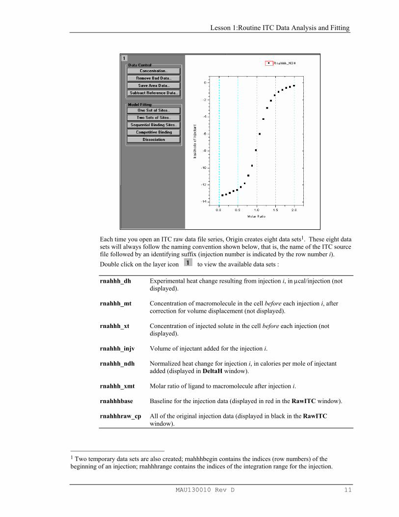
Each time you open an ITC raw data file series, Origin creates eight data sets1. These eight data sets will always follow the naming convention shown below, that is, the name of the ITC source file followed by an identifying suffix (injection number is indicated by the row number i). Double click on the layer icon to view the available data sets :
rnahhh_dh Experimental heat change resulting from injection i, in µcal/injection (not
displayed). rnahhh_mt Concentration of macromolecule in the cell before each injection i, after
correction for volume displacement (not displayed). rnahhh_xt Concentration of injected solute in the cell before each injection (not
displayed). rnahhh_injv Volume of injectant added for the injection i. rnahhh_ndh Normalized heat change for injection i, in calories per mole of injectant
added (displayed in DeltaH window). rnahhh_xmt Molar ratio of ligand to macromolecule after injection i. rnahhhbase Baseline for the injection data (displayed in red in the RawITC window). rnahhhraw_cp All of the original injection data (displayed in black in the RawITC
window).
1 Two temporary data sets are also created; rnahhhbegin contains the indices (row numbers) of the beginning of an injection; rnahhhrange contains the indices of the integration range for the injection.

ITC Tutorial Guide
12 MAU130010 Rev D
Origin creates three worksheets to hold these data sets. To open these worksheets refer to Lesson 5, which describes how to open worksheets from plotted data, copy and paste data, and export data to an ASCII file. Now would be a good time to save the area data (the RNAHHH integration results) as a separate data file. We will use this data again in Lesson 4 when we subtract reference data.
To save area data to a separate file
• Select Window:DeltaH to make DeltaH the active window. Alternatively, you may
press and hold the Ctrl key and press the tab key to scroll through Origin's open windows.
• Click on the Save Area Data button Origin opens the File Save As dialog box, with Rnahhh.DH selected in the File name text box.
• Select a folder for the file and click OK. Before fitting a curve to the data, it is a good idea to check the current concentration values for this experiment.
To edit concentration values
• Click on the Concentration button in the DeltaH window.
• A dialog box opens showing the concentration values for the RNAHHH data.
Click OK or Cancel to close the dialog box. You should always check that the concentration values are correct for each experiment. Incorrect values will negate the fitting results. If you need to edit the concentration values, simply enter a new value in the appropriate text box. The concentration and injection volume values which appear initially are those which the operator enters before the experiment starts. The cell volume is a constant which is stored in the data collection software. This value is read by Origin whenever you call up an ITC data file.

Lesson 1:Routine ITC Data Analysis and Fitting
MAU130010 Rev D 13
Before you proceed to fit the data, you may want to manually adjust baselines or integration details. These procedures are discussed in Lesson 2, but here we will simply accept the computer-generated results.
Curve Fitting
Origin provides six built-in curve fitting models: One Set of Sites, Two Sets of Sites, Sequential Binding Sites, Competitive Binding, Dissociation and Enzyme Assays. To invoke one of these models, click on the appropriate button in the DeltaH window. The following describes the basic procedure for fitting a theoretical curve to your data. See Lesson 7 for advanced curve fitting lessons, and the Appendix for a discussion of fitting equations.
To fit the area data to the One Set of Sites model
• Click anywhere on the DeltaH plot window to make it the active window. Or select DeltaH from the Window menu.
• Click on the One Set of Sites button.
A new command menu display bar appears. The Fitting Function Parameters dialog box opens (there are two modes for the Fitting Sessions dialog box, basic and advanced, see page 58 for more information), showing initial values for the three fitting parameters for this model - N, K, and H. Origin initializes the fitting parameters, and plots an initial fit curve (as a straight line, in red, please see page 101 for a discussion of line types) in the DeltaH window.
• Click 1 Iter. or 100 Iter. button in the Fitting Session dialog box to control the iteration
of the fitting cycles. Click 1 Iter. to perform a single iteration, 100 Iter. to perform up to 100 iterations. It may be necessary that the 100 Iter. command be used more than once before a good fit is achieved. Repeat this step until you are satisfied with the fit, and Chi^2 is no longer

ITC Tutorial Guide
14 MAU130010 Rev D
decreasing. Note that the fitting parameters in the dialog box update to reflect the current fit.
Fitting Parameter Constraints
Each fitting model has a unique set of fitting parameters. For the One Set of Sites model these are N (number of sites), K (binding constant in M-1), and ∆H (heat change in cal/mole). A fourth parameter, ∆S (entropy change in cal/mole/deg), is calculated from ∆H and K and displayed after fitting. You can use the Fitting Session dialog box to apply mathematical constraints to the fitting parameters. We mention this subject only in passing, for a detailed discussion see page 59 and the appendix.
To hold a parameter constant The Vary? column in the Fitting Session dialog box contains three checkboxes, one associated with each fitting parameter. If a box is check marked, Origin will vary that parameter during the fitting process in order to achieve a better fit. To hold a parameter constant during iterations, click in the box to remove the checkmark from the checkbox.
Fitting Parameters Text
To copy and paste the fitting parameters to the DeltaH window
Once you have a good fit, click on the Done.. button and the fitting parameters will be automatically pasted into a text window named Results Log and to the DeltaH window in a text label. This label is a named object (called Fit.P) that is linked to the fitting process through Origin's label control feature (For more information see the Origin User's Manual or for online help, right click anywhere in the text label and select Label Control… then press the F1 key ). Position and format this label just as you want the fitting parameters to appear. When you paste the fitting parameters, they will replace the "Fit Parameters" label, but retain its position and style. Origin will use any text label named Fit.P to display the fitting parameters. To name a text label, click on the label once to select it, select Format:Label Control, and enter a name in the Object Name text box in the Label Control dialog box.
Data: Rnahhh_NDH Model: OneSites Chi^2/DoF = 2856 N 1.02±0.0016 K 5.54E4 ±1.1E3 ∆H -1.361E4 ±29.8 ∆S -22.0

Lesson 1:Routine ITC Data Analysis and Fitting
MAU130010 Rev D 15
To format the fitting parameters text
• Right-click anywhere in the text box and select Properties item from the drop down menu. The
Text Control dialog box will appear allowing you to format the fitting parameters text.
The Text Control dialog box is in three sections. The upper section contains various formatting options. The middle contains the text box where the desired text, with formatting options, are entered. The lower view box provides a WYSIWYG (What You See Is What You Get) display of the text entered into the middle text box. Hint: Press the F1 key while the Text Control dialog box is open for Online help and a thorough description of text formatting options. • Use the controls to format the text.. Select Black Line from the Background drop-
down list box to change the background style from shadow to border (to remove the background style altogether, select (None) from the Background drop down list. If the background line is not removed, it may be necessary to select Window:Refresh). Click OK when done. The DeltaH window redraws to show the changes in the text box.
To move the text in the plot window
• Click once on the text in the plot window.
• A colored outline appears, indicating that the text is selected and the cursor will change
into an arrow headed cross.

ITC Tutorial Guide
16 MAU130010 Rev D
• Slowly Click again,within the colored outline, to move the text.
• Click outside the colored outline to deselect the text.
Hint: If you click anywhere along the edge of the text background border, a colored size box appears around the text with various size boxes positioned around the perimeter. Click and drag on one of the small perimeter boxes to change the size of the text background frame. Origin will automatically change the font size to fit within the size of the box. Note that any formatting changes can be saved as part of the DeltaH plot window template file. See page 49 for details.
To view the Results Log
Origin automatically routes most analysis and fitting results to the Results Log (a sub window of Origin's Project Explorer). In most cases, when results are output to the Results Log, it opens automatically (although it may be positioned out of view, docked to the lower edge of the workspace). However, to manually open (and Close) the Results
Log, click the Results Log button on the standard toolbar. Opening and closing the Results Log only controls its view state. You do not lose results by closing the log. When the Results Log first opens, it displays docked to the lower edge of the workspace. You can dock it to any other edge or display it as a window in the workspace. To prevent the Results Log from docking when positioning it it as a window, press CTRL while dragging.
Each entry in the Results Log includes a date/time stamp, the window name, a numeric stamp which is the Julian day, the type of analysis performed, and the results.
Please refer to the Origin User's Manual or on-line help for more information about the Results Log and Project Explorer
When you save an Origin project, the contents of the Results Log is saved with the project.

Lesson 1:Routine ITC Data Analysis and Fitting
MAU130010 Rev D 17
Creating a Final Figure for Publication
To create a final figure for publication, select Final Figure from the ITC menu. The ITCFINAL plot window opens. This window contains two related graphs. The top graph shows raw data in terms of µcal/second plotted against time in minutes, after the integration baseline has been subtracted. The bottom graph shows normalized integration data in terms of kcal/mole of injectant plotted against molar ratio. The two X axes are linked, so that the integrated area for each peak appears directly below the corresponding peak in the raw data.
-40
-20
0
0 10 20 30 40
Time (min)
µcal
/sec
0.0 0.5 1.0 1.5 2.0-14
-12
-10
-8
-6
-4
-2
0
Molar Ratio
kcal
/mol
e of
inje
ctan
t
Note: The user should understand that the "raw data" in the upper frame of the ITCFinal template is the original raw data after the integration baseline has been subtracted from it. Once this subtraction has been made by creating the ITCFinal figure, there is no way to recover the original raw data except by starting a new project and calling in the raw data file again, since the subtracted data has been stored under the original filename and the original integration baseline replaced by the Y=0 baseline.
If you modify the integration data or the fit curve in the DeltaH window, or the raw data in the RawITC window, simply select Final Figure again to update the ITCFINAL window with your changes. Note that the top graph in the ITCFINAL window still includes the integration baseline at Y = 0. You may wish to remove this baseline before printing the graph.
ITC Tutorial Guide
18 MAU130010 Rev D
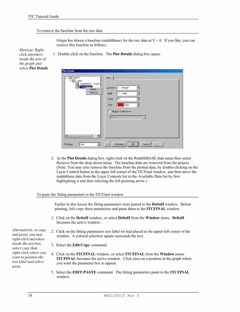
To remove the baseline from the raw data Origin has drawn a baseline (rnahhhbase) for the raw data at Y = 0. If you like, you can remove this baseline as follows:
1. Double-click on the baseline. The Plot Details dialog box opens.
2. In the Plot Details dialog box, right-click on the RnahhhBASE data name then select Remove from the drop down menu. The baseline data are removed from the project. (Note: You may also remove the baseline from the plotted data, by double-clicking on the Layer Control button in the upper left corner of the ITCFinal window, and then move the rnahhhbase data from the Layer Contents list to the Available Data list by first highlighting it and then selecting the left-pointing arrow.)
To paste the fitting parameters to the ITCFinal window
Earlier in this lesson the fitting parameters were pasted to the DeltaH window. Before printing, let's copy these parameters and paste them to the ITCFINAL window.
1. Click on the DeltaH window, or select DeltaH from the Window menu. DeltaH becomes the active window.
2. Click on the fitting parameters text label we had placed in the upper-left corner of the window. A colored selection square surrounds the text.
3. Select the Edit:Copy command. 4. Click on the ITCFINAL window, or select ITCFINAL from the Window menu.
ITCFINAL becomes the active window. Click once on a position in the graph where you want the parameter box to appear.
5. Select the EDIT:PASTE command. The fitting parameters paste to the ITCFINAL
window.
Shortcut: Right-click anywhere inside the axis of the graph and select Plot Details
Alternatively, to copy and paste, you may right-click anywhere inside the text box, select copy then right-click where you want to position the text label and select paste.

Lesson 1:Routine ITC Data Analysis and Fitting
MAU130010 Rev D 19
6. We want to position the text label next to the integration data, but first we need to reduce the size of the label. Right-click inside the text box then select Properties… from the drop down menu to open the Text Control dialog box. Select 10 (or type 10) in the Size drop-down list to reduce the point size to 8. Click OK to close the dialog box.
7. Click and drag the label to position it next to the integration data, as shown below:
To print the final figure
To print the page in the ITCFINAL window, select Print from the File menu. Before you print, make sure ITCFINAL is the active window. When a window is active its title bar changes from gray to blue (this can vary depending on your Windows setup, to view or change your setup select Start:Settings:Control Panel then double click on Display and click on the Appearance tab). Click on a window to make it active, or select the window from the Window List in the Window menu.
To save the project and exit
• Choose Save Project As... from the File menu. The file Save As dialog box opens.
• Enter a name for the project (for example, Lesson 1) in the File Name text box. The name for the project may contain up to 255 characters and include spaces.
Shortcut: Click the Save Project button on the Standard toolbar.
0.0 0.5 1.0 1.5 2.0
-14
-12
-10
-8
-6
-4
-2
0
0 10 20 30 40
-50-45-40-35-30-25-20-15-10-505
Data: Rnahhh_NDHModel: OneSitesChi^2/DoF = 2856N 1.02 ±0.0016K 5.54E4 ±1.1E3∆H -1.361E4 ±29.8∆S -22.0
Time (min)
µcal
/sec
Molar Ratio
kcal
/mol
e of
inje
ctan
t

ITC Tutorial Guide
20 MAU130010 Rev D
• Click on the Save button.
The entire contents of this project (including all data sets and plot windows) are saved into a file called Lesson 1.OPJ.
• Choose Exit from the File menu. Origin closes.

Lesson 2: Setting Baseline and integration Range
MAU130010 Rev D 21
Lesson 2: Setting Baseline and Integration Range
In Lesson 1 you learned how to use Origin to perform routine data analysis of ITC files. In routine data analysis, integration details (baselines and integration ranges) are determined automatically. Sometimes, however, the automatically determined values are not sufficiently accurate, and you will want to set integration details manually. This is especially true when working with very small injection peaks. This lesson shows you how to manually set integration details. Begin this lesson by starting Origin, then opening the RNAHHH. ITC data file, as you did at the beginning of Lesson 1.
To start Origin
• Double-click on the MicroCal, LLC ITC icon on the DeskTop. (If the icon is not
available on the DeskTop, Start from the task bar, then select Programs: OriginLab:MicroCal LLC ITC). Origin opens and displays a new project with the RawITC template plot window.
To open the RNAHHH file • Click on the Read Data button. The Open dialog box opens, with the ITC Data (*.it?)
file name extension selected. • If you have not previously Set Default Folder... to the samples subfolder, then navigate
to the C:\Origin70\samples subfolder. • Select Rnahhh from the Files list. • Click OK.
• Raw data are plotted in the RawITC window. Normalized area data are plotted in the
DeltaH window. • Select the RawITC window from the file list in the Window menu.
Note: If you ever notice that the the RawITC window , or another window, has lost some of its formatting instructions (e.g., text rotation), this can happen from being in the Draft View mode. Draft View is the fastest view mode, and is very useful when precise formatting is not required. The View Mode is selected from the Page menu. To view the page as it will appear when printed, select Page View mode which is the slowest but most accurate. Page View mode is often the most useful, since it combines reasonably good WYSIWYG accuracy with fast operation. (also see Origin User’s Manual or Origin’s Help menu item, for more information on view mode).
To enter the Adjust Integration session
• Click on the Adjust Integrations button in the RawITC window. The cursor changes into a cross hair.

ITC Tutorial Guide
22 MAU130010 Rev D
• Move the cursor into the RawITC plot window and click on or near the injection peak
you want to adjust. For this example, click on peak 19 (second peak from the right). The window zooms to shows the baseline region of peaks 18, 19 and 20. (Note: Origin will show the injection peak before and the injection peak after the injection chosen, but any manipulations will only affect the integrated area between the center injection)
A new set of buttons appears along the top edge of the window. Two blue lines appear,
the section of the plot between the lines is the integration range.
The basic procedure for adjusting integration details is to select a peak, adjust the baseline and the integration range, integrate the peak, and then move on to the next peak and repeat the process. The expanded screen is shown below.
To adjust the baseline
• Click on the Baseline button in the RawITC window (which has been temporarily titled Peak 19). The automatically generated points for this baseline appear. (For the baseline, Origin displays 15 points which includes the central peak and each neighboring peak. In most cases you may want to adjust only the central five points for the central peak of interest. The outermost points are usually more closely associated with the neighboring peaks. Click on a point, then drag the mouse or use the ↑ and ↓ keys to move the point (note that baseline points can only move vertically). Use the ← and →keys (or the mouse) to select the next point to the right or left. Repeat for each point you want to move. Note: When any point on the baseline is moved, the position of the moved point automatically becomes part of the baseline and any future integration will be calculated from this new baseline.

Lesson 2: Setting Baseline and integration Range
MAU130010 Rev D 23
(Note: For a closer look you may use the Magnifying Glass from the Toolbox to expand the flat baseline portion of your data for more accurate adjustment of the integration baseline. To do this, click on the appropriate icon in the Toolbox. Then place the icon pointer near the indicated position 1 in the above figure, click and drag it to position 2 shown above. When you release the mouse button, that part of the graph contained within the solid rectangle will expand to fill the plot window for better viewing of the baseline. If you wish to return to the original non-expanded display, double-click on the Magnifying Glass icon or proceed on to integrate the next peak. If you wish to keep the same expanded Y axis limits for integrating other peaks, then double-click on the Y axis to bring up the Y Axes Dialog Box (see below). Click on the Scale tab then in the lower left corner of the dialog box, change the Rescale option from Normal to Manual and click OK. Now the Y axis will maintain these limits and will not rescale when you proceed on to adjust integration for other peaks. ) Contact MicroCal if you wish to permanently change the default values for the y-axis scaling.
• Once the baseline is where you want it, you may press the escape key (or the Enter
key) to set the baseline. The data points will disappear and the cursor will change from the cross hair to the pointer tool so you may adjust the integration range. If the

ITC Tutorial Guide
24 MAU130010 Rev D
integration range is already set you may click on the Integrate button and click on an arrow key to show an adjacent peak
To adjust the integration range
• If the baseline data points are still visible double-click on any data point or press the
Enter key or press the Esc key. The data points will disappear and the cursor will change from the cross-hair to the pointer tool.
• Set a new integration range by clicking and dragging either line with the mouse.
• The integration area for the central peak selected will be between the dashed blue lines.
To integrate the selected peak • Click on the Integrate button.
This integrates the peak, using the current baseline and integration range. The curve in the DeltaH window is updated accordingly. The integration results are also updated on the worksheet containing the injection data.
To select another peak
• Click on the and buttons to move to the next or
previous peak. Note that the current peak number is always displayed in the window title bar.
To end the Adjust Integration session
• Click on the Quit button. The RawITC window is restored to show all of the injection peaks. Note that the area data in the DeltaH window will have updated to reflect any changes you made.

Lesson 2: Setting Baseline and integration Range
MAU130010 Rev D 25
You will notice that the RawITC template includes a button to Integrate All Peaks. This button integrates all injection peaks and replots the area data. You will recall from the previous lesson that the area data in the DeltaH window were originally created with the Integrate All Peaks routine. It is not necessary at this point to integrate on all peaks again. In fact, it is a good idea not to. If you now integrate on all peaks, you will not get the same area result as when you integrated each peak separately.
To view the worksheet data • Select the Pointer tool by clicking on it in the Toolbox.
• Double-click anywhere on the trace of the RawITC data plot in the plot window or select Format : Plot. The Plot Details dialog box opens for this data plot.
• Click on the Worksheet button. The Worksheet containing the injection data opens.
Note: You may notice that the worksheet X axis values are in seconds, while the plotted data is shown in minutes. This is because the X axis has been factored, as described in Lesson 6. You can now proceed to fit the data (see Lesson 1). If necessary, you can first delete any bad data points, as descried in the next lesson.
Shortcut to the Worksheet: Right-click anywhere on the data trace and select Open Worksheet.

ITC Tutorial Guide
26 MAU130010 Rev D
This page was intentionally left blank

Lesson 3: Deleting Bad Data
MAU130010 Rev D 27
Lesson 3: Deleting Bad Data
After your injection data are integrated, the integration results are displayed in the DeltaH plot window. You can delete bad data points from the DeltaH window before starting the fitting session.
To delete bad data points
• Select Window : DeltaH to make it the active window. • Click on the Remove Bad Data button.
The pointer becomes a cross-hair. • Click on the point that you want to delete.
A small red cross appears on the selected data point. The XY coordinates, index number, and data set name for the selected point are displayed immediately in the Data Display Tool (floating). Note: If you have trouble selecting a particular data point, select a point near by and use the left or right arrow keys to move to the data point you wish to select.
• Press ENTER.
The selected data point is deleted. Alternatively, after clicking on Remove Bad Data, you may double click on a data point to delete it. Note: The main menu bar also contains a data deletion function under Data: Remove Bad Data Points… and this works a little differently. We recommend the user always delete data using the Remove Bad Data button located on the DeltaH plot window. Though there is no Undo command available in this version of Origin with which to un-delete a data point, it is possible to recover if you have mistakenly deleted a point. To recover, simply integrate the injection peaks again (by clicking on the Integrate All Peaks button in the RawITC window). All of the injection peaks will re-integrate, and the area data, including the deleted data point, will replot in the DeltaH window. A second way to recover the bad point, without reintegrating, is to click on the Concentration button and then click OK. Even if you did not change the concentration in the dialog box, Origin goes back to the worksheet and normalizes on the concentration again which then restores the deleted point.
Shortcut to switch between Origin windows: Press and hold down the Ctrl key while pressing the Tab key.

ITC Tutorial Guide
28 MAU130010 Rev D
This page was intentionally left blank

Lesson 4: Analyzing Multiple runs and subtracting Reference
MAU130010 Rev D 29
Shortcut: Click the New Project button on the Standard toolbar.
Lesson 4: Analyzing Multiple Runs and Subtracting Reference Origin allows you to open multiple runs of ITC data into the same project, and subtract one run from another. The heat of ligand dilution into buffer can thus be subtracted from the reaction heat by performing the control experiment of injecting into a buffer solution, and subtracting this reference data from the reaction heat data. In order to subtract the reference injections, you must have both the sample and reference area data in memory. This lesson shows you how to read two area data files into Origin and subtract one from the other. In the first example below you will read two area (.DH) data files from disk. In the second example, you will work directly with two raw (*.ITC) ITC data files. This second example also illustrates some helpful procedures for dealing with difficult data Two reference data files, BUFFER.DH and FEBUF10.ITC, have been included in the [samples] subfolder for your use with this lesson. Before you begin this lesson, open a new project. This will clear any old data that may be in memory.
To open a new project
• Choose Project from the New sub-menu under the File menu.
Opening Multiple Data Files
In the following example you will open two area (.DH) data files and subtract one from the other. Both area files were previously saved to disk. This example assumes that you have previously opened the ITC file Rnahhh.itc into Origin, and saved the resulting area data as Rnahhh.DH, as described in Lesson 1. If you have not yet done so, you should refer to Lesson 1 now.
To read the sample and reference data into memory
• Click on the Read Data.. button in the RawITC plot window.
The File Open dialog box opens click on the down arrow in the Files of type: drop-down list box and select Area Data (*.DH).
• Navigate to the C:\Origin70\samples subfolder.
Several .DH files will be listed in the File Name list box.

ITC Tutorial Guide
30 MAU130010 Rev D
• Double-click on Rnahhh.dh. Alternatively you can single click and click Open. The Rnahhh.dh file opens, the data are normalized on concentration, then the data are plotted in the DeltaH window, as a scatter plot called Rnahhh_ndh. Rnahhh_ndh shows area data as kilo-calories per mole of injectant plotted against molar ratio.
The Rnahhh_NDH normalized area data.
0.0 0.5 1.0 1.5 2.0
-14
-12
-10
-8
-6
-4
-2
0
Rnahhh_NDH
Molar Ratio
kcal
/mol
e of
inje
ctan
t

Lesson 4: Analyzing Multiple runs and subtracting Reference
MAU130010 Rev D 31
• Return to the RawITC template and repeat the above steps to open the reference data file Buffer.dh. Buffer.dh is also located in the [samples] subfolder.
A new plot, Buffer_ndh, replaces Rnahhh_ndh in the DeltaH window.
The Buffer_ndh normalized buffer data. When you open the second ITC data file Buffer_ndh, the Rnahhh_ndh data are cleared from the DeltaH plot window. The Rnahhh_ndh data have not been deleted from the project, but are simply removed from the window display. Since the data are not deleted, they can be retrieved from memory and replotted.
To show both the sample and the reference area data
• Double-click on the layer 1 icon , at the top left corner of the DeltaH window. The Layer Control dialog box opens.
• Click on Rnahhh_ndh in the Available Data list, then click on the => button.
Rnahhh_ndh copies to the Layer Contents list.
Shortcut to Layer Control: Right-click on any white space between the axis and select Layer Contents…
0.0 0.5 1.0 1.5
-0 .25
-0 .20
-0 .15
-0 .10
-0 .05
0.00
B uffer_N D H
M olar R atio
kcal
/mol
e of
inje
ctan
t

ITC Tutorial Guide
32 MAU130010 Rev D
• Click OK. Rnahhh_ndh plots into the DeltaH window. The axes automatically rescale to show all of the data.
Rnahhh_ndh and Buffer_ndh, plotted together.
The Available Data list in the Layer Control dialog box shows all data sets currently available for plotting in this project. The Layer Contents list shows all data sets currently plotted in the active layer. See the Origin User’s Manual or Origin's Online Help menu item (or press F1) for more on handling Origin data.
0.0 0.5 1.0 1.5 2.0
-14
-12
-10
-8
-6
-4
-2
0
Buffer_NDH
Rnahhh_NDH
Molar Ratio
kcal
/mol
e of
inje
ctan
t

Lesson 4: Analyzing Multiple runs and subtracting Reference
MAU130010 Rev D 33
Note that you can read any number of data files into the same DeltaH window. When multiple data plots appear in the same window, you can set the active data plot by clicking on the plot type (line/symbol) icons next to the data set name in the legend: A black border around the line/symbol icon indicates the currently active data plot. Editing, fitting, and other operations can only be carried out on the active plot.
Adjusting the Molar Ratio
Note in the above figure that the Buffer_ndh data plots from molar ratio 0 to ca. 1.3, while the Rnahhh_ndh data plots from 0 to ca. 2.0. In the case of the Buffer_ndh data, the molar ratio is in fact infinity since injections of 21.16 mM ligand solution were made into a cell which contained only buffer and no macromolecule (i.e., in order to determine heats of dilution of ligand into buffer). Origin automatically assigns a concentration of 1.0 mM in order to obtain non-infinite values for the molar ratio to allow plotting of the Buffer_ndh points. Before subtracting the reference data you should check that the molar ratio is identical for both data sets. This will ensure that the final result is accurate, and will also ensure that the two data sets plot in register (that is, injection #1 of the control experiment plots at the same molar ratio as injection #1 of the sample experiment, etc.).
To adjust the molar ratio
1. Click on the Data menu, and check that Rnahhh is checkmarked. If not, select Rnahhh from the menu. This sets Rnahhh as the active data set.
(as a simpler alternative to the above procedure, you could have just clicked on the Rnahhh_NDH listing in the plot type icon.)
2. In the DeltaH window, click on the Concentration button. In the dialog box that opens, note the value in the C in Cell (mM) field (it should be 0.651).
3. Click Cancel to close the dialog box. Now repeat step 1, but this time set the Buffer data
set as active.
Alternatively you may right-click on any open space between the axis and click on Rnahhh

ITC Tutorial Guide
34 MAU130010 Rev D
4. In the DeltaH window, click again on the Concentration button. This time a dialog box opens to show the concentration values for Buffer. In the C in Cell (mM) field, enter 0.651. Click OK. The two data sets will now plot in register, as shown below:
Subtracting Reference Data
To subtract Buffer_ndh from Rnahhh_ndh • Click on the Subtract Reference Data.. button in the DeltaH window.
The Subtract Reference Data dialog box opens. The most recent file opened, in this case Buffer_NDH, will appear in both the Data and Reference drop down list box. Note that the data set in the Reference box will be subtracted from the data set in the Data box.
• Select Rnahhh_NDH from the Data drop down list. Rnahhh_NDH becomes highlighted and will be entered as the Data.

Lesson 4: Analyzing Multiple runs and subtracting Reference
MAU130010 Rev D 35
• Click OK.
Every point in Buffer_ndh is subtracted from the corresponding point in Rnahhh_ndh. The result is plotted as Rnahhh_ndh in the active layer, in this case layer 1 in the DeltaH plot window.
Note that Buffer_ndh is not affected by this operation. It is cleared from the DeltaH window, but is still listed as available data in the Layer Control dialog box. The Original Rnahhh_ndh data could be recovered by selecting Math : Simple Math and adding the Buffer_ndh data set to the new Rnahhh_ndh data set.
To save the project and all related data files
• Select the File:Save Project As command from the Origin menu bar.
The Save As dialog box opens, with untitled selected as the file name.
• Enter a new name (Origin7.0 accepts long filenames) for the project, navigate to the folder in which you want to save the file, and click OK. It is not necessary to enter the .opj file extension. This will be added automatically. Now that you have named the file, the next time you save it you can simply use the File:Save Project command. In order to save some memory space, you may find it useful to delete the original injection data. This may be useful when you are reading a large number of data sets into the same Origin project.
0.0 0.5 1.0 1.5 2.0-14
-12
-10
-8
-6
-4
-2
0
Rnahhh_NDH
###
Molar Ratio
kcal
/mol
e of
inje
ctan
t

ITC Tutorial Guide
36 MAU130010 Rev D
To delete a data set from a project, either • Double-click on any layer icon in any plot window.
• Select a data set from the Available Data list, then click on the Delete button.
or
• If the data are plotted in a plot window, double-click on the trace of the data plot that you
want to delete. The Plot Details dialog box opens. The name of the data set appears in the file list box under the layer icon.
• Right-click on the file name you wish to delete then click Delete from the drop down menu.
In either case the data set, along with any related data plots, is deleted from the project. If you have saved the data set to disk, the saved copy will not be affected.
Plotting Multiple Data Sets Whenever multiple data sets are included in the same plot, there may be overlap of data points from the different data sets. There are two ways to eliminate this overlap by displacing one or more of the curves on the Y axis if you wish to do so. First, you may select Math : Simple Math and add or subtract a constant from all points in one data set to displace it. Remember if you are doing this on data plotted in the DeltaH template that although data is plotted in kcal, the actual data is in the worksheet as cal so they must be modified by adding or subtracting cal (see A Note about Units starting on page 53). Second, you may make the appropriate data set active by selecting it in the list for plot type icons. Then select Math : Y Translate. Use the resulting cross-hair icon to select one data point in the active set , click on it, and hit enter (or double click on a data point). Then move the icon to the Y position on the graph where you wish that point to be after displacement, click on it and hit enter. The entire data set will be translated on the Y axis by that amount.
Subtracting Reference Data: Additional Topics
In the previous example, the sample injection data and reference injection data matched precisely. This may not always be the case, however. Your reference data may have a different number of injections than your sample data, or the injection time spacing may differ between the two runs. You will see below how to deal with these situations. In the following example you will open two ITC raw (*.ITC) data file series, one containing the sample data and one containing the reference data. You will then plot the area data for each data file series, and subtract reference data from sample data. Begin by opening a new project:
• Select File:New:Project and click OK.

Lesson 4: Analyzing Multiple runs and subtracting Reference
MAU130010 Rev D 37
To open both sample and reference raw data files • Click on the Read Data.. button in the RawITC window and select ITC Data (*.it?)
from the Files of type: drop down list.
• Double-click on Rnahhh in the File Name list (located in the [Origin70][samples] subfolder). The Rnahhh.itc file opens. The data are integrated, normalized, and the area data plots in the DeltaH window.
• Return to the RawITC window and repeat the above steps to open the Febuf10.itc data file.
• The Febuf10_ndh area data replaces Rnahhh_ndh in the DeltaH window. You need to plot both area data sets into layer 1.
To show both area data sets in layer 1
• Double-click on the layer 1 icon in the DeltaH plot window. The Layer Control dialog box opens.
• Select Rnahhh_ndh in the Available Data list, then click on the => button. Rnahhh_ndh joins Febuf10_ndh in the Layer Contents list.
• Click OK.
Rnahhh_ndh joins Febuf10_ndh in the DeltaH plot window. The axes automatically rescale to show all the data. Your plot window should now look like the illustration below:
As we discussed earlier in this lesson (page 33), you should now check that the ligand concentrations for both data sets are identical. Make each data set active in turn, then

ITC Tutorial Guide
38 MAU130010 Rev D
click on the Concentration button in the DeltaH window, and check that value in the C in Cell (mM) field for Febuf10_ndh is identical to that value for Rnahhh_ndh. In this case, you will find that the two values are the same. Notice that Febuf10_ndh shows only twelve injections, while Rnahhh_ndh shows twenty. How do you subtract one data set from another when the number of injections doesn't match? The quick and dirty way is to subtract a constant. A more precise method would be to fit a straight line to the reference data, then subtract the line. Let's look briefly at each method.
To subtract a constant from Rnahhh_ndh
• Select the Data Reader tool from the toolbox. The pointer changes to a cross-hair.
• Click the mouse on several different data points in the Febuf10_ndh data series in the DeltaH window, each time noting the Y value that appears in the Data Display.
• Using these Y values, figure a rough average for the data. For this example, let's say the average Y value is 350 (See Calculating a Mean Value for Reference Data starting on page 103 for a method to quickly calculate a mean of the data). (Note that the Data Reader tool shows values in calories, while the Y axis in this graph shows values in kcal. This is because the Y axis in the DeltaH plot window template is factored by a value of 1000. See Lesson 6 for more about factoring.)
• Select Simple Math from the Math menu. The Math on/between Data Set dialog box opens.
• Select Rnahhh_ndh from the Available Data list, then click on the uppermost => button.
• Rnahhh_ndh copies to the Y1 text box. Rnahhh_ndh also appears next to Y:. Y: indicates the name of the data set into which the resulting data will be copied. Click in the Y2 text box and type " 350 " at the insertion point. Click in the operator box, and type " - " at the insertion point.

Lesson 4: Analyzing Multiple runs and subtracting Reference
MAU130010 Rev D 39
• Click OK.
The constant "350" is subtracted from each value in the Rnahhh_ndh data set. The result is plotted as Rnahhh_ndh in the DeltaH window.
To subtract a straight line from RNAHHH_NDH
• Click on the Pointer tool to deselect the Screen Reader tool. Now check the Data menu to see that Febuf10_ndh is the active data set (the active data set will be checkmarked). All editing, and fitting operations are carried out on the active data set. Select Febuf10_ndh if it is not active.
• Select Linear Regression from the Math menu. A straight line is fit to the Febuf10_ndh data. Origin assigns the name LinearFit_Febuf10ND to the data set for this line.

ITC Tutorial Guide
40 MAU130010 Rev D
• Select Simple Math from the Math menu.
The Math dialog box opens.
• Select Rnahhh_NDH from the Available Data list, then click on the uppermost => button. Rnahhh_NDH copies to the Y1 text box.
• Select LinearFit_Febuf10ND from the Available Data list, then click on the lowermost => button. LinearFit_Febuf10ND copies to the Y2 text box.
• Click in the operator box and type " - ".
• Click OK.
Every point in LinearFit_Febuf10ND is subtracted from the corresponding point in Rnahhh_ndh. The resulting data set is plotted as Rnahhh_ndh in the DeltaH plot window. Note that the Febuf10_ndh reference data plot (the original twelve injection points) is not affected.

Lesson 4: Analyzing Multiple runs and subtracting Reference
MAU130010 Rev D 41
We will end this lesson with a note about injection timing. You may have noticed the difference in injection time spacing between Rnahhhraw_cp and Febuf10raw _cp. To make this difference more apparent you need to plot both raw data sets in the same plot window.
To plot both Rnahhhraw_cp and Febut10raw_cp in the RawITC plot window • Click on the RawITC window to make it active (or select RawITC from the Window
menu).
• Double-click on the layer 1 icon in the RawITC window. The Layer Control dialog box opens for layer 1.
• Select rnahhhraw_cp in the Available Data list, then click on the => button. rnahhhraw_cp is added to the Layer Contents list.

ITC Tutorial Guide
42 MAU130010 Rev D
• Click OK.
Both rnahhhraw_cp and febuf10raw_cp are now plotted in the RawITC window. Note the difference in the time spacing of the injections.
The difference in peak spacing is not a problem when subtracting reference data. You can work with data files having different time spacing, since you are interested primarily in the integration area data for each peak.
0.00 8.33 16.67 25.00 33.33 41.67 50.00-70
-60
-50
-40
-30
-20
-10
0
Time (min)
µcal
/sec

Lesson 5: ITC Data Handling
MAU130010 Rev D 43
Lesson 5: ITC Data Handling
Every data plot in Origin has an associated worksheet. The worksheet contains the X, Y and, if appropriate, the error bar values for the plot. A worksheet can contain values for more than one data plot.
It is always possible to view the worksheet from which data were plotted. This lesson shows you how to open the worksheet associated with a particular data plot, copy/paste the data, export the data to an ASCII file, and import ASCII data.
Reading Worksheet Values from Plotted Data
Begin this lesson by opening the ITC Rnahhh.ITC data file series, as follows:
• Select File : New : Project. A new Origin project opens to display the RawITC plot window.
• Click on the Read Data.. button.
The File Open dialog box opens, with the ITC Data (*.IT?) file name extension selected.
• If you have not previously Set Default Folder... to the samples folder, then navigate to
the C:\Origin70\samples folder. • Select Rnahhh from the file name list, and click OK.
As you saw in Lesson 1, Origin plots the Rnahhh data as a line graph in the RawITC plot window, automatically creates a baseline, integrates the peaks, normalizes the integration data, and plots the normalized data in the DeltaH plot window. As a result, the following eight data sets are created: rnahhh_dh Experimental heat change resulting from injection i, in
µcal/injection (not displayed). rnahhh_mt Concentration of macromolecule in the cell before each
injection i, after correction for volume displacement (not displayed).
rnahhh_xt Concentration of injected solute in the cell before each injection (not displayed).
rnahhh_injv Volume of injectant added for the injection i. rnahhh_ndh Normalized heat change for injection i, in calories per mole of
injectant added (displayed in DeltaH window). rnahhh_xmt Molar ratio of ligand to macromolecule after injection i (X
value of data point). rnahhhbase Baseline for the injection data (displayed in red in the
RawITC window). rnahhhraw_cp All of the original injection data (displayed in black in the
RawITC window). In addition origin creates two temporary data sets:
Shortcut: Select the New Project button.

ITC Tutorial Guide
44 MAU130010 Rev D
rnahhhbegin Contains the indices (row numbers) of the start of an injection. rnahhhrange Contains the indices of the integration range for the injections. An Origin data set is named after its worksheet and worksheet column, usually separated by an underscore. Thus the first six data sets above will all be found on the same worksheet (RNAHHH), in columns named DH, INJV, Xt, Mt, XMt and NDH, respectively. The temporary two data sets above are located on separate worksheets, named rnahhhbase (an Origin created baseline) and RnahhhRAW (the experimental data). The temporary data sets are indices created by Origin and do not have a worksheet created.
To open the Rnahhh worksheet
• Select the Plot... command from the Format menu.
The Plot Details dialog box opens for the rnahhh_ndh data plot (if the DeltaH window is active).
• Click on the Worksheet button. The Rnahhh worksheet opens. Please note: If a worksheet cell is not wide enough to display the entire number, Origin will fill the cell with ###### signs. The full number is used by Origin. If you wish to view the full number you may increase the column width, by placing the cursor on the left or right border of the column name, waiting till the cursor changes to a double headed arrow, then moving the column edge to the left or right to increase the column width. Alternatively you may right-click the column name select properties from the drop-down list and increase the value in the Column Width text box.
Shortcut to worksheet: Right-click on the data trace and select Open Worksheet.

Lesson 5: ITC Data Handling
MAU130010 Rev D 45
Copy and Paste Worksheet Data
Data can be copied from a worksheet to the clipboard, then pasted from the clipboard into another Origin worksheet, a plot window, or another Windows application. To copy and paste worksheet data:
Select a range of worksheet values • Select the initial cell, row, or column in the range.
To select a cell, click on the cell. To select an entire row, click on the row number. To select an entire column, click on the column heading.
• To select a contiguous portion of worksheet values, click on the first cell, row or column, keep the mouse button depressed, drag to the final cell, row, or column that you want to include in the selection range, then release the mouse button. The entire selection range will now be highlighted. (Note: If you ever wish to select a range of cells where the initial cell but not the final cell is in view, then click on the first cell and scroll to the final cell, press and hold the shift key then click the final cell.
Copy the selected values to the clipboard
• Choose Copy from the Edit menu, alternatively you may click the right mouse button inside the highlighted text and select Copy from the menu. The selected values are copied to Windows clipboard.
Select a destination for the copied values • To paste into a plot window, click on the plot window to make it active. • To paste into a worksheet, click on the worksheet (or select File:New:Worksheet to
open a new worksheet), then click to select a single cell. This cell will be in the upper left corner of the destination range.
Shortcut: To open a new worksheet click on the New Worksheet button from the Standard toolbar.

ITC Tutorial Guide
46 MAU130010 Rev D
• To paste into another Windows application, switch to the target application, then follow the pasting procedure for that application. (Shortcut: If an application is already open you may switch to it by pressing and holding down the Alt key then pressing the Tab key till the application's icon is selected.
Paste the copied values from the clipboard to the destination
• Select Paste from the Edit menu, alternatively click the right mouse button and select Paste. The selected values are pasted from the clipboard. Note: It may happen that your worksheet does not show the data, but only displays pound signs, as shown on the right. The data is available for manipulations but is not displayed because the column is not wide enough. You may increase the column width by moving the cursor to the right edge of the column header (the cursor will change into a double headed arrow) then clicking and dragging the cursor to the right or you may right click the column heading, select properties, then increase the number for the column width.
Exporting Worksheet Data
The contents of any worksheet can be saved into an ASCII file. In this section you will open the worksheet for the RnahhhBASE baseline data plotted in the RawITC window, and export the X and Y data to an ASCII file.
To open the Rnahhhbase worksheet
• Click on the RawITC window (or choose RawITC from the Window menu) to make it
the active window. • Select RnahhhBASE from the Data menu.
RnahhhBASE becomes checkmarked to show it is selected.
• Select Plot... from the Format menu.
The Plot Details dialog box opens.
• Click on the Worksheet button. The RnahhhBASE worksheet opens.
Shortcut to worksheet: Right-click on the data trace and select Open Worksheet.

Lesson 5: ITC Data Handling
MAU130010 Rev D 47
To export the worksheet data as an ASCII file • Select Export ASCII... from the File menu.
The Export ASCII dialog box opens, with RnahhhBASE.DAT selected as the file name.
• Click Save. • After you click Save in the Export ASCII dialog box, the ASCIII Export Into dialog box
opens.
Shortcut: Right-click on the upper left containing white-space then select Export ASCII.

ITC Tutorial Guide
48 MAU130010 Rev D
• You may format the output of this ASCII file (Please refer to the Origin User's Manual for more information about Exporting worksheet data). This file may then be opened into any application that recognizes ASCII text files.
Importing Worksheet Data
ASCII files can be imported directly into an Origin worksheet or plot window. The basic worksheet Origin menu supports a number of additional file formats for importing data (Lotus, Excel, dBASE, LabTech, etc.) while the menus for ITC or DSC Data Analysis support routine ASCII import.
To import an ASCII file into a new worksheet
• Choose Worksheet from the New sub-menu under the File menu. A new Origin worksheet, Data1, opens.
• Select the File : Import : ASCII command. (If you like, you can select File : ASCII : Options. This will allow you to set ASCII file import options.) The Import ASCII dialog box opens, set to open a data file with a .DAT extension.
• Double-click on a file in the File Name list (for example, the RnahhhBASE.DAT file you just exported). The RnahhhBASE data imports into the worksheet.
To import an ASCII data file into a plot window • Choose Graph from the New sub-menu under the File menu. • Choose Import ASCII: Single File from the File menu. • Select the rnahhhBASE.dat ASCII file from the Files list. Enter the appropriate Initial
X Value (0 for RnahhhBASE.dat) and Increment in X (28.25287) and click OK.
Shortcut: To create a graph, click on the New Graph button from the Standard toolbar

Lesson 6: Modifying Templates
MAU130010 Rev D 49
Lesson 6: Modifying Templates
The RawITC, DeltaH, and ITCFinal plot windows (and all other plot windows in Origin) are created from template files (*.OTP file extension). A template file is a file that contains all of the attributes of a plot window (or a worksheet) except the data. The important thing about template files is that you can change a plot window, and then save the changes into the template file for that window. The next time you open the window it will include your changes. Thus template files let you customize plot windows to meet your specifications. You can change any of Origin's template files. In this lesson we will edit both the DeltaH and ITCFinal plot windows, then save the changes into the corresponding template file. Though the changes we make will be minor, you can actually change any property of a template. For more information about customizing templates, refer to the Origin User’s Manual or press the F1 key for Online Help. Caution: In this lesson you will be modifying plot window templates that are basic to Origin's operation. In the unlikely event that you make a mistake you are unable to correct, simply copy the original template file from the Custom folder of the installation CD-ROM. This will correct any problem that may arise.
Modifying the DeltaH Template
The DeltaH template shows units of kilocalories/mole of injectant along the left Y axis. The scale for this axis is actually defined in terms of calories/mole of injectant, but the axis is factored by 1000 to yield units of kilocalories/mole. The right Y axis labels for the DeltaH template are hidden from view. In the following example we will modify the template so that the right Y axis labels are visible. We will then factor the labels by 1000, so they will be identical to the left Y axis labels, and then save these changes into the DeltaH template file.
To open the DeltaH plot window • If you are continuing from a previous lesson click on the New Project button from the
Standard toolbar or select Project from the New sub-menu under the File menu to create a new project.
• Click on the Read Data.. button in the RawITC window
The File Open dialog box opens, with the ITC Data (*.ITC) file extension selected.
• Navigate to the C:\Origin70\Samples folder and open any ITC data file (for example, FEBUF10.ITC). The DeltaH template opens to show the normalized area data.
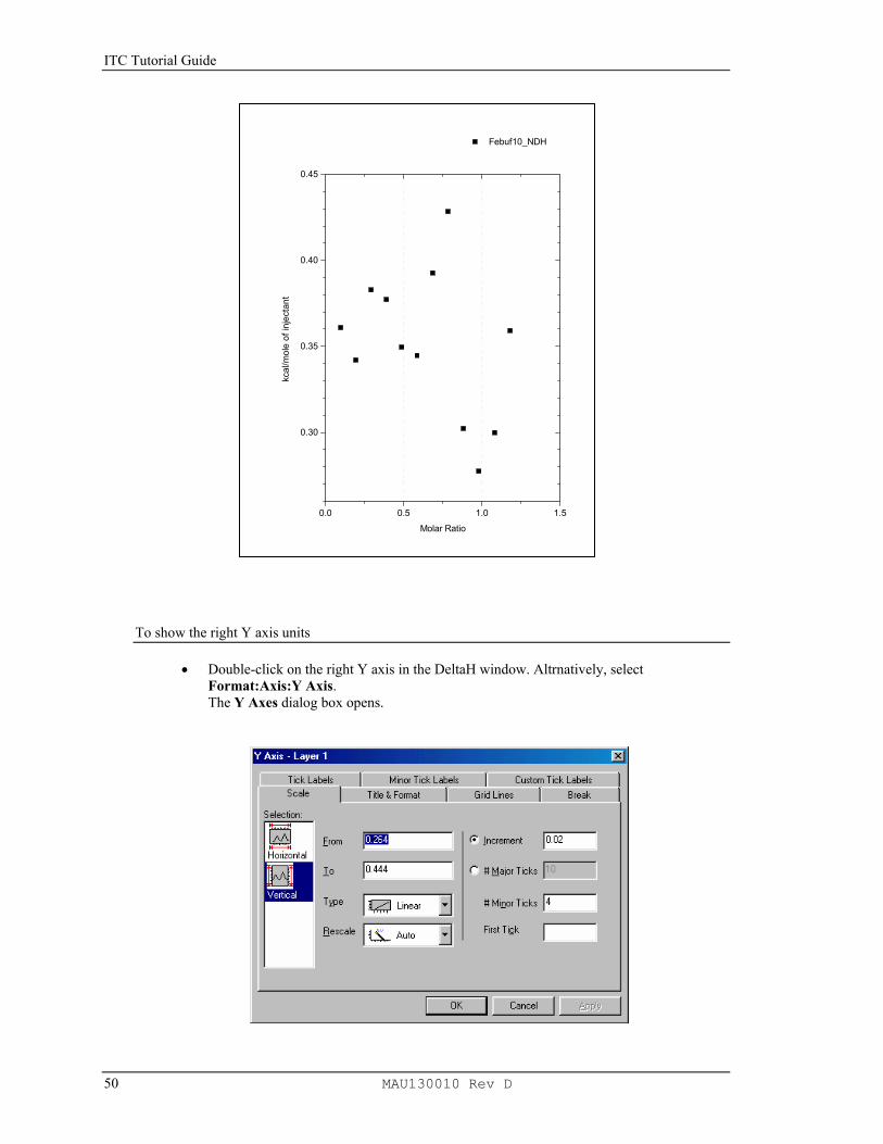
ITC Tutorial Guide
50 MAU130010 Rev D
To show the right Y axis units
• Double-click on the right Y axis in the DeltaH window. Altrnatively, select Format:Axis:Y Axis. The Y Axes dialog box opens.
0.0 0.5 1.0 1.5
0.30
0.35
0.40
0.45
Febuf10_NDH
Molar Ratio
kcal
/mol
e of
inje
ctan
t
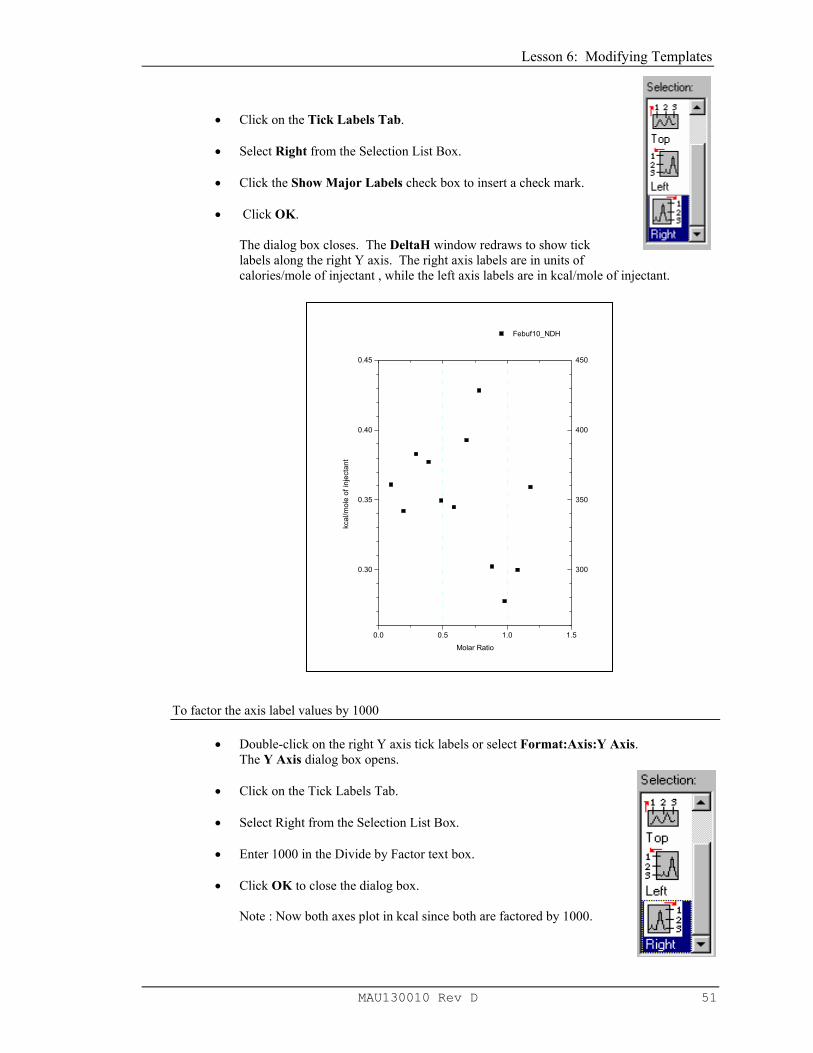
Lesson 6: Modifying Templates
MAU130010 Rev D 51
• Click on the Tick Labels Tab.
• Select Right from the Selection List Box.
• Click the Show Major Labels check box to insert a check mark. • Click OK.
The dialog box closes. The DeltaH window redraws to show tick labels along the right Y axis. The right axis labels are in units of calories/mole of injectant , while the left axis labels are in kcal/mole of injectant.
To factor the axis label values by 1000
• Double-click on the right Y axis tick labels or select Format:Axis:Y Axis. The Y Axis dialog box opens.
• Click on the Tick Labels Tab.
• Select Right from the Selection List Box.
• Enter 1000 in the Divide by Factor text box.
• Click OK to close the dialog box.
Note : Now both axes plot in kcal since both are factored by 1000.
0.0 0.5 1.0 1.5
0.30
0.35
0.40
0.45
300
350
400
450
Febuf10_NDH
Molar Ratio
kcal
/mol
e of
inje
ctan
t

ITC Tutorial Guide
52 MAU130010 Rev D
To save the changes into the DeltaH template file
• Select File:SaveTemplate As…. Origin opens a dialog box asking if you want to save the file as DELTAH.OTP (the DeltaH template file).
• Click Cancel at this point if you do not want to change the original DeltaH template. If you click OK, Origin will save the modified DeltaH window as DELTAH.OTP. If you saved the modified template and now select the File:Read Data.. buttonthe modified DeltaH window will appear. Note that plotted data cannot be saved to a template file, so there is no need to delete the plotted area data before saving the DeltaH window.
To revert to the original DeltaH template If you do decide to modify the DeltaH template, it is easy to recreate the original. Simply reverse the steps you used to create the modified template. That is, open the DeltaH window, open the Y-Axis dialog box, click on the Tick Labels tab, remove the check mark from the Show Major Labels check box, then select File: Save Template As…
Modifying the RawITC template
The RawITC plot window shows bottom X axis tick labels in units of minutes. Let's use what we have just learned about factoring tick labels to change this axis scale so that the tick labels are in units of hours rather than minutes.
To factor the RawITC X axis tick labels by 3600 • Set the RawITC window as the active window (by either pressing and holding the Ctrl
key then pressing the Tab key, or selecting RawITC from the Window menu).
• Double-click on the bottom X axis tick labels or select Format:Axis:X Axis. The X Axis dialog box opens.
• Click on the Tick Labels Tab.
• Select Bottom from the Selection List Box.
• Enter 3600 in the Divide by Factor text box. Since the worksheet X values for raw ITC data are in terms of seconds, a factor of 3600 gives us axis tick label values in units of hours for this axis.
• Set Decimal Places to 2.
Shortcut: Click on the Save Template icon from the Standard toolbar.
Shortcut: Right-click on the bottom X-axis tick labels and select Tick Labels from the drop down menu list
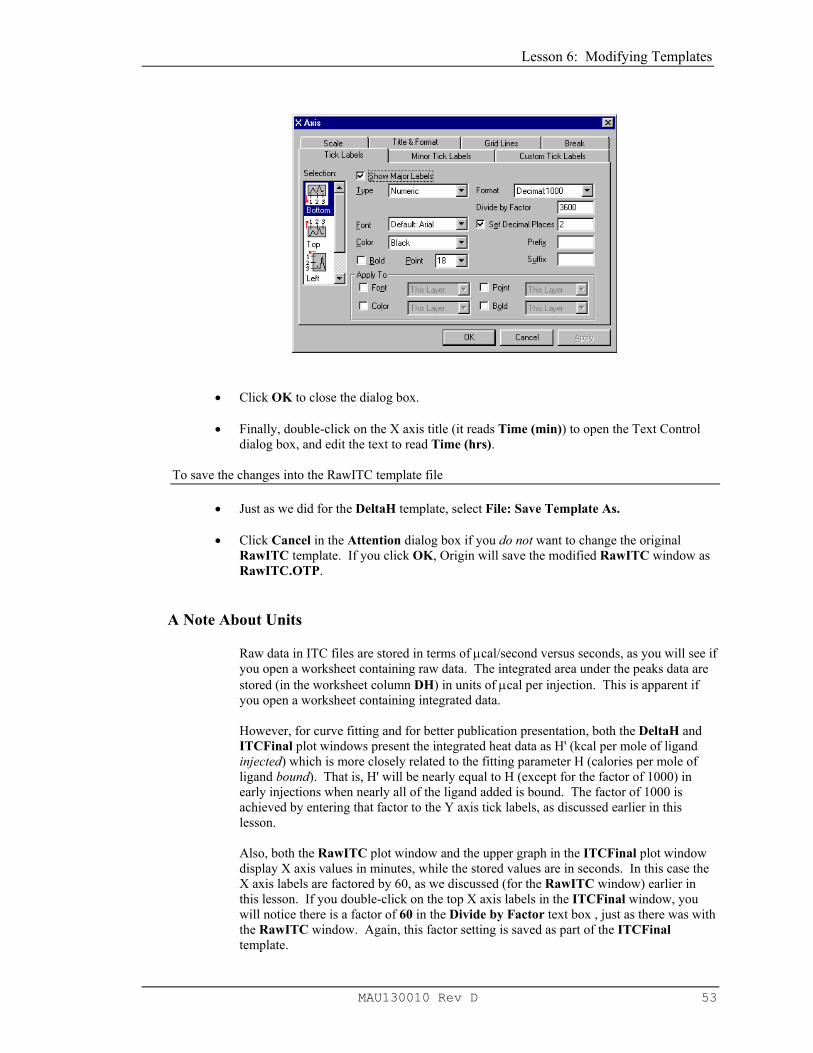
Lesson 6: Modifying Templates
MAU130010 Rev D 53
• Click OK to close the dialog box.
• Finally, double-click on the X axis title (it reads Time (min)) to open the Text Control dialog box, and edit the text to read Time (hrs).
To save the changes into the RawITC template file • Just as we did for the DeltaH template, select File: Save Template As.
• Click Cancel in the Attention dialog box if you do not want to change the original
RawITC template. If you click OK, Origin will save the modified RawITC window as RawITC.OTP.
A Note About Units
Raw data in ITC files are stored in terms of µcal/second versus seconds, as you will see if you open a worksheet containing raw data. The integrated area under the peaks data are stored (in the worksheet column DH) in units of µcal per injection. This is apparent if you open a worksheet containing integrated data. However, for curve fitting and for better publication presentation, both the DeltaH and ITCFinal plot windows present the integrated heat data as H' (kcal per mole of ligand injected) which is more closely related to the fitting parameter H (calories per mole of ligand bound). That is, H' will be nearly equal to H (except for the factor of 1000) in early injections when nearly all of the ligand added is bound. The factor of 1000 is achieved by entering that factor to the Y axis tick labels, as discussed earlier in this lesson.
Also, both the RawITC plot window and the upper graph in the ITCFinal plot window display X axis values in minutes, while the stored values are in seconds. In this case the X axis labels are factored by 60, as we discussed (for the RawITC window) earlier in this lesson. If you double-click on the top X axis labels in the ITCFinal window, you will notice there is a factor of 60 in the Divide by Factor text box , just as there was with the RawITC window. Again, this factor setting is saved as part of the ITCFinal template.

ITC Tutorial Guide
54 MAU130010 Rev D
The Y axis data plotted in the DeltaH and lower ITCFinal templates (i.e., data with .ndh extension) are normalized on moles of injectant. If you ever wish to view the experimental integrated heats in µcal per injection, then double-click on the Layer dialog box, and move the _ndh file out of the Active data and move the _dh file into the Active data. To complete the process, you must double-click on the Y axis tick labels and remove the factor of 1000.

Lesson 7: Advanced Curve Fitting
MAU130010 Rev D 55
Lesson 7: Advanced Curve Fitting
The model for one set of sites discussed in Lesson 1 will work for any number of sites n if all sites have the same K and ∆H. If a macromolecule has sites with two different values of K and/or ∆H, then the model with two sets of sites must be used. Whenever there are two sets of sites, the automatic initialization procedure is rarely effective. If the initialization parameters are extremely far away from best values, then convergence to the best values cannot take place as iterations proceed. In fact, often the fit gets worse rather than better with successive iterations. Therefore, the user must get involved in arriving at initialization parameters before the iterations can be started. An indication of poor initialization occurs when values for the K parameter become negative during the fitting procedure.
Fitting with the Two Sets of Sites Model
The protein ovotransferrin has two very tight, non identical sites for binding ferric ions; one located in the N domain and one in the C domain. The Origin area data FeOTF54.NDH shown below were obtained by titrating ovotransferrin with ferric ion. Injections 1-5 titrate primarily the stronger N site, injections 7-11 primarily the C site, while injections 13-15 result in no binding since both sites are already saturated. • Select File:New:Project (or click on the New Project button) to create a new
project. Click on the Read Data.. button in the RawITC window and select Area Data (*.DH) from the File of type drop down list, go to the C:\Origin70\Samples folder, and open FeOTF54.DH.
0.0 0.5 1.0 1.5 2.0 2.5 3.0
-12
-10
-8
-6
-4
-2
0
2
Feotf54_NDH
Molar Ratio
kcal
/mol
e of
inje
ctan
t

ITC Tutorial Guide
56 MAU130010 Rev D
• Now click on the Two sets of Sites button in the DeltaH window. Origin opens the
NonLinear Curve Fitting: Fitting Session dialog box, but produces an attention dialog box and a very poor initial fit to the curve. Click OK in the warning dialog to proceed.
You will see that the auto initialization produces a curve which represents the data very poorly. If iterations are started from this, the fit will not converge. A little intuition, however, will allow the operator to obtain a satisfactory initialization which will lead to convergence. Examination of the experimental points shows that the first few injections at a molar ratio below 1 produce ca. 1 kcal per mole of injectant, changing to ca. -12 kcal for molar ratio 1 to 2 and finally changing to zero at molar ratios larger than 2. Begin manual initialization then by entering 1 into both the N1 and N2 parameter boxes in the Fitting Session dialog box. Because of the behavior noted above, H1 must be near +1000 and H2 close to -12,000, so enter these guesses into the appropriate parameter boxes. Since the experimental heats fall off quickly from the H1 value to the H2 value, it is clear that K1 must be much larger than K2, and because the heat changes abruptly from the H2 value to zero (i.e., beginning with the eleventh injection) it is also clear that K2 itself must be large (i.e., even though it is smaller than K1). Enter 1e8 into the K1 parameter box, and 1e6 into the K2 parameter box. Be careful not to insert a space before or after the e when using exponential notation, or Origin will not accept the value.

Lesson 7: Advanced Curve Fitting
MAU130010 Rev D 57
Click on the Chi-Sqr button in the dialog box. Origin draws a new fit curve using the entered parameters, which is a much better representation of the data.
Though this fit is good enough to lead to correct convergence, we can still improve on it some. Since the fit curve goes from H2 to zero much more gradually than the data, let's increase K2 from 1e6 to 1e8. We must still keep K1 larger than K2, so increase K1 from 1e8 to 1e10. Click on Chi-Sqr button and observe that we now have a very good initialization curve. Select the 100 Iter. button a few times, and convergence occurs with a final chi^2 of about 33,000.

ITC Tutorial Guide
58 MAU130010 Rev D
Note that N1 and N2 are nearly the same magnitude, but not quite. It would be interesting to see if a fit of nearly equal quality could be obtained with N1 and N2 exactly equal to each other. (Although theoretically they should each be 1.0. Assign the value 1.0 into the N1 and N2 parameter value box, click in the N1 and N2 checkboxes to remove the checkmark, and continue the iterations. The final fit is not as good as when N1 and N2 are both floated, although there is no obvious explanation for this. Float all variables (by replacing the checkmark for N1 and N2) and iterate until you return to the earlier fit with a chi^2 of about 33,000. Note that sometimes you may have to click on the 10 Iter. command many times before you achieve the smallest chi^2 value, as the fitting can become trapped in a local minimum for several iterations. Click on the Done button to end the fitting session
NonLinear Least Squares Curve: Fitting Session
Two NLSF Modes: Basic and Advanced Origin offers two modes of its nonlinear least squares fitter, Basic and Advanced. While both modes allow you to fit your data, they differ substantilallly in the options they provide as well as in the degree of complexity.
By default, when you enter the NLSF Curve Fitting Session by selecting one of the three ITC curve fitting models, the Origin's nonlinear least squares fitter starts in the mode most recently used.
Basic Mode
Allows for performing iterative curve fitting to the built in functions and plotting the results to the graph. Click on the More… button to enter the Advanced mode.
Advanced Mode
In addition to the basic mode features the Advanced Mode allows for defining linear constraints, adjusting the configuration of the fitting parameters, simulating data and defining your own fitting function. Click on the Basic Mode button to return to the Basic mode.
Aborting the NLSF Session If you wish to exit the NLSF session without printing the fitting parameters to the Results window or the graph text box, select the fitting session dialog box close button and click No to the dialog box question: Do you want to end the current fitting session?
For more information on the Fitting Session, press the F1 after opening the dialog box.
Basic Mode
Advanced Mode

Lesson 7: Advanced Curve Fitting
MAU130010 Rev D 59
Controlling the Fitting Procedure
You may enter the NLSF Curve Fitting Session and initialize the parameters by selecting one of the three fitting models (One Set of Sites, Two Sets of Sites or Sequential Binding Sites). After the parameters have been determined you may re-enter the NLSF Curve Fitting Session and keep the same fitting parameters by selecting from the menu, Math : Start Fitting Session. Normally the Fitter will open in the Basic mode, click on the More… button to enter the Advanced Mode of the Fitter. From the Fitting Session window, select Options:Control to open the Control Parameters dialog box. Edit this dialog box to specify several quantitative properties (as described below) of the fitting procedure. These properties directly affect the way the fitter performs iterations.
The Control Parameters Dialog Box
The Tolerance Text Box MicroCal has preset this value to be 0.05, but you may type a new value for the tolerance in this text box. When you click 'n Iter' in the Fit Session dialog box, this causes the fitter to try to perform, at most, n Levenberg-Marquardt (LM) iterations. If the relative change of the value of chi-square between two successive iterations is less than the value in the Tolerance text box, less than n iterations are performed. If you want the fitter to perform still more iterations, click on either the n Iter or the 1 Iter button in the Fitting Session dialog box. The value, 100, is specified as 'n' in the Max. Number of Iterations text box (see below).

ITC Tutorial Guide
60 MAU130010 Rev D
The Max. Number of Iterations Drop-down List Specify the value for the maximum number of iterations performed when the n Iter button is clicked on in the Fitting Session dialog box. This has been preset by MicroCal to be 100, but the user may change this number to be effective during a session of Origin, by entering a new value in the text box. However, the value will be reset to 100 after exiting Origin.
The Derivative Delta Group This group determines how the fitter will compute the partial derivatives with respect to parameters for ITC fitting functions during the iterative procedure. If the Fixed Delta check box is unchecked (recommended for ITC users), then the actual value of Delta (derivative step size) for a particular parameter is equal to the current value of the parameter times the value specified in the Delta text box. The Maximum and Minimum text boxes specify the limiting values of the actual Delta, in case a parameter value becomes too large or too small. MicroCal has preset the Delta to be .06 with the limiting maximum to be 5 x 10+30 and the minimum to be 5 x 10-30. If your fit curve is not converging well you may want to try a different value for the Delta, for ITC users this is typically a larger value (e.g. 0.07, 0.08, etc). The new value will be valid for the current session of Origin, but will default back to .01 the next time Origin for ITC is opened. Contact MicroCal, if you need to permanently change the Delta value.
The Parameters Significant Digits Group Select values for the display of significant digits for each parameter from the associated drop-down list. Select Free from the drop-down list to use the current Origin setting. This will only effect the text box display in the Fitting Sessions dialog box. MicroCal has preset the significant digits to be 4 for all parameters.
The Weighting Method Drop-Down List The bottom part of the Control Parameters dialog box enables you to select how different dataset points are to be weighted when computing chi-square during the iterative procedure. The choices are: No weighting, Instrumental, Statistical, Arbitrary dataset, and Direct Weighting. We recommend that the default option of No weighting be used for all ITC data unless the user has strong reason to feel another choice is more appropriate for a particular data set. No weighting assumes that each data point has the same absolute error probability. Return to the Fitting Session dialog box by clicking on the button or by selecting Action : Fit.
Deconvolution with Ligand in the Cell and Macromolecule in the Syringe
Whenever the ligand and macromolecule each have only one site for interaction with the other, then the system is symmetrical, and it does not matter which of the two is loaded into the cell and which into the injection syringe. The operator must only be careful to record the proper concentration of the species in the syringe and the species in the cell. In cases where the ligand is sparingly soluble and the macromolecule is not, then it is sometimes advantageous to load the ligand into the cell since the starting concentration then need not be so high. The situation is a little more complicated if the macromolecule has more than one site (even if there is only one set of sites). Let's assume that it has two fairly strong sites with differing affinity for ligand. If we put the macromolecule in the cell and the ligand in the

Lesson 7: Advanced Curve Fitting
MAU130010 Rev D 61
syringe, then the tightest of the two sites with heat change H1 will titrate in the early injections and the weakest of the two with heat change H2 will titrate in subsequent injections until both sites are saturated, whereupon the heat change goes to zero. However, if the ligand is loaded into the cell and the macromolecule in the syringe, then the situation is different, since the ligand will be in excess in the early injections so that both sites will titrate with heat change H1 + H2. Once sufficient macromolecule (i.e., molar ratio of macromolecule/ligand of 0.5) has been added to tie up all of the ligand as the 2-to-1 complex, then further injections of the apo-macromolecule will result in some of the ligand being removed from the weaker site in the 2-to-1 complex so that it can bind to the stronger site on the newly-injected macromolecule. The heat change for this second phase of the titration will then be H1 - H2, assuming that site 1 is sufficiently stronger than site 2. This being the case, then all of the ligand will be in the 1-to-1 complex when the molar ratio reaches 1.0, and further injections of macromolecule will give zero heats. For example, take a look at the ITC integration data file OTFFe3.DH. To open this file, first click Done! in the fitting session menu bar to exit from the fitting session, then select File:New:Project (or click on the New Project button) to create a new project. Now click on the Read Data.. button in the RawITC window, select Files of type: Area Data (*.DH), then navigate to the C:\Origin70\Samples folder, then double-click on OTFFe3 in the File Name list. The normalized (.NDH) data plot into the plot window.
The data in file OTFFe3.DH were obtained with the macromolecule (ovotransferrin) in the syringe and the ligand (a chelated form of ferric ion) in the cell. Injections 1-5 correspond to formation of the diferric form of ovotransferrin with heat change H1 + H2. Injections 8-14 involve conversion of the diferric form into the mono ferric form with heat change H1 - H2.
• Before fitting to this data, select Ligand is in (Cell) from the ITC menu.

ITC Tutorial Guide
62 MAU130010 Rev D
• Click OK in the Attention dialog box.
This switches the settings, letting Origin know that the ligand is now in the cell. You may confirm this by clicking on the ITC menu again and noting that the checkmark is next to Ligand is in (Cell). (Note: Origin defines the "macromolecule" as the species with n greater than 1.0 and the "ligand" as the species with only one site, irrespective of their molecular weights.)
Now you can click on the Two Sets of Sites button to select the appropriate fitting model. The default fitting parameters will lead to a satisfactory convergence in this case but lets try to improve on them before beginning interations. The first several injections indicate that H1 + H2 equals about -10,000 calories per mole. You might start off with values of -7000 for H1 and -3000 for H2. Set n1 and n2 equal to 1.0,, and click to remove the N1and N2 checkmark. Insert 1e8 for K1 and 1e6 for K2. Select Chi-Sqr, and use the 100 Iter. command to iterate until chi^2 no longer changes. Notice that the estimated errors for K1 and K2 are quite large, being about 100% in the case of K1. To verify this, change the K1 value from ca 3.2E7 to 5E7, remove the checkmark from K1, and carry out 30 iterations. Replace the checkmark at K1 and click on Chi-Sqr, which then shows a value of ca 32000. Click on 100 Iter. again, note that the original K1 value of ca 3.2 x 10⁷ has reappeared, and that the new Chi-Sqr value is only slightly smaller at ca 31000. Thus the two fits having very different fit parameter values, have approximately the same Chi-Sqr. This is because these data show rather large scatter from the smooth theoretical fit curve and are therefore not capable of defining precise values for the fitting parameters. You may run across other instances in your own experiments when fitting parameters are even more poorly defined than for OTFFe3.DH. The most likely situation for this to occur is with two sets of sites, where K1 and K2 values are less than 10-fold different. It is even possible that the set of "best fit" parameters may be quite different depending on the initialization parameters which are used to start the fit; i.e., the curve-fitting routine can become trapped in a local minimum for chi^2 and be unable to find the global minimum. You can usually detect this by starting with several different sets of initialization parameters to see if you arrive at the same final minimum with nearly the same fitting parameters. When you are satisfied with the fit, click on the Done button in the dialog box to paste the fitting parameters to the Results Window, the plot window and end the fitting session. Go to the ITC menu, and reselect the default option, Ligand is in (Syringe)

Lesson 7: Advanced Curve Fitting
MAU130010 Rev D 63
Deconvolution with the Sequential Binding Sites Model
All models discussed until now are concerned only with independent sites. It often occurs in biological systems that the binding of a ligand to one site will be influenced by whether or not ligands are bound to any of the other sites. If the sites happen to be non-identical in the first place, then binding studies alone cannot determine whether the sites are independent or interacting. On the other hand, if the sites within a molecule are known to be identical, then it is possible, sometimes, to determine if they are interacting. Consider the simplest case, that of a macromolecule with two identical sites; this might be a homodimeric protein, for example. If the sites are identical, then we can no longer distinguish between binding at the first site and binding at the second site, so the bookkeeping must be done in terms of the first ligand bound (K1, H1) and the second ligand bound (K2, H2), as described in the Appendix. A system with positive cooperativity means K2>K1, while negative cooperativity means K1>K2. Positive cooperativity is generally more difficult to distinguish from binding studies alone, since the tendency is for both sites on any single molecule to saturate together with heat change H1 + H2, so that only one "phase" is seen in the titration curve. To determine if cooperativity were present, one could use another technique which was able to show that, at half saturation, the dominant molecular forms were the macromolecule with either two or no ligands attached, with very little of the singly-liganded form. Negative cooperativity can be more easily detected from binding studies, since there will be two different "phases" occurring: the strong binding of the first ligand and the weaker binding of the second. The Origin file protb.dh shows integrated heat data on a macromolecule with two identical sites. If you have not done so yet click on Done! in the Fitting Sessions window to exit. Then select File:New:Project (or click on the New Project button) to open a new project. To open protb.dh, click on the Read Data.. button in the RawITC window, then select Area Data (*.dh) from the File of Type: drop down box. Go to the C:\Origin70\Samples sub-folder, and double-click on protb.dh.
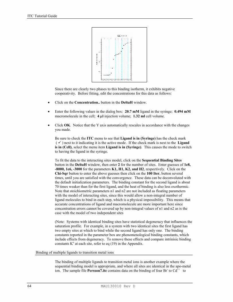
ITC Tutorial Guide
64 MAU130010 Rev D
Since there are clearly two phases to this binding isotherm, it exhibits negative cooperativity. Before fitting, edit the concentrations for this data as follows:
• Click on the Concentration.. button in the DeltaH window. • Enter the following values in the dialog box: 20.7 mM ligand in the syringe; 0.494 mM
macromolecule in the cell; 4 µl injection volume; 1.32 ml cell volume.
• Click OK. Notice that the Y axis automatically rescales in accordance with the changes you made. Be sure to check the ITC menu to see that Ligand is in (Syringe) has the check mark ( ) next to it indicating it is the active mode. If the check mark is next to the Ligand is in (Cell), select the menu item Ligand is in (Syringe). This causes the mode to switch to having the ligand in the syringe. To fit the data to the interacting sites model, click on the Sequential Binding Sites button in the DeltaH window, then enter 2 for the number of sites. Enter guesses of 1e8, -8000, 1e6, -3000 for the parameters K1, H1, K2, and H2, respectively. Click on the Chi-Sqr button to enter the above guesses then click on the 100 Iter. button several times, until you are satisfied with the convergence. These data can be deconvoluted with the default initialization parameters. The binding constant for the second ligand is about 70 times weaker than for the first ligand, and the heat of binding is also less exothermic. Note that stoichiometric parameters n1 and n2 are not included as floating parameters with the model of interacting sites, since this would allow a non-integral number of ligand molecules to bind in each step, which is a physical impossibility. This means that accurate concentrations of ligand and macromolecule are more important here since concentration errors cannot be covered up by non-integral values of n1 and n2 as is the case with the model of two independent sites (Note: Systems with identical binding sites have statistical degeneracy that influences the saturation profile. For example, in a system with two identical sites the first ligand has two empty sites at which to bind while the second ligand has only one. The binding constants reported in the parameter box are phenomenological binding constants, which include effects from degeneracy. To remove these effects and compare intrinisic binding constants Ko at each site, refer to eq (19) in the Appendix.
Binding of multiple ligands to transition metal ions The binding of multiple ligands to transition metal ions is another example where the sequential binding model is appropriate, and where all sites are identical in the apo-metal ion. The sample file Persson7.itc contains data on the binding of four Br- to Cd++ to

Lesson 7: Advanced Curve Fitting
MAU130010 Rev D 65
form CdBr4--. For practice call up the file and do curve fitting to obtain binding
parameters for each of the four bromide ions using the Sequential Binding Sites model. The concentrations of both Br- and Cd++ are correct as contained in the file. Convergence occurs (you must click on 100 Iter.. button several times) without operator selection of initial parameters, but you may want to try to improve the initialization for practice.
Using the Sequential Binding model with non-identical sites The model of Sequential Binding can also be useful for systems with non-identical sites. The Two Sets of Sites model, discussed earlier, considers the saturation of individual sites on the same molecule, assumes they saturate independently of one another, and uses three fitting parameters for each site; N, K and H. The model of Sequential Binding Sites assumes a fixed sequence of binding, i.e., the first ligand which binds to an individual molecule always binds to site 1, the second ligand which bids to an individual molecule always binds to site 2, etc. The number of sequential sites must be exactly integral (1,2,3,…) so there is no fitting parameter equivalent to N, and best-fit is determined by only two parameters, K and H, at each site once the total number of sites has been selected by the operator. For a molecule which has 2 sites of quite different affinity (e.g., K values different by a factor of five or more) the two models will tend to give equivalent values of K and H since thermodynamics will dictate binding to the site of highest affinity first. However, when K values at two independent sites are more nearly equivalent, then sequential binding will not be strictly followed.
0 2 4 6 8 10 12
0
2
Data: Persson7_NDHModel: Sequential Binding SitesChi^2/DoF = 50.98K1 2.34E3 ±37∆H1 -318.7 ±6.33∆S1 14.4K2 114 ±5.0∆H2 4565 ±125∆S2 24.6K3 2.22E3 ±99∆H3 1119 ±141∆S3 19.0K4 25.0 ±0.86∆H4 -6690 ±75.1∆S4 -15.9
Persson7_NDH Persson7_B
Molar Ratio
kcal
/mol
e of
inje
ctan
t
ITC Tutorial Guide
66 MAU130010 Rev D
One inherent advantage of the sequential model is the smaller number of fitting parameters for each site. Using a model for independent sites, it would be extremely difficult to obtain a unique fit for more than two sets of sites - which is why no fitting model for three sets of independent sites has been included in this software. As shown above for the Persson7.itc file, the sequential model is capable of providing a unique fit even for systems with four binding sites (if the K and/or H values are sufficiently different for each site). Thus, for some multi-site systems the model of sequential binding may be the only choice available for providing a unique phenomenological characterization of binding parameters..
Enzyme/substrate/inhibitor Assay
There are two different methods described below for carrying out an enzyme assay. These methods are discussed in the Appendix, where the appropriate equations are included. Both methods assume that no significant product inhibition occurs. In Method 1, an enzyme solution is in the sample cell and the experiment consists of a single injection of substrate solution into the sample cell. Immediately after injection the calorimeter baseline shifts prominently to reflect heat effects which occur from the decomposition of substrate as it comes into contact with the enzyme (because of the finite response time of the instrument, it takes a few minutes before the calorimetric signal becomes equilibrated with the actual heat from substrate turnover). Eventually, after all substrate has been reacted, the baseline will return to its original position prior to injection of substrate. From analysis of the decay curve resulting from substrate decomposition, the Michaelis parameters KM (mM)and Kcat (sec-1) may be determined as well as the heat of substrate decomposition ∆H. If a second similar experiment is carried out but with an inhibitor in the sample cell along with the enzyme, then the resulting decay curve may be analyzed in a similar way to determine the Michaelis inhibitor constant KI (mM). In the analysis of this second decay curve, the parameters determined in the first experiment (KM, Kcat and ∆H) are used as input parameters and only KI is used as a fitting parameter. In Method 2, the enzyme solution is again placed into the reaction cell but the enzyme concentration will generally be lower than in method 1. A number of injections of substrate solution are carried out, allowing baseline equilibration to occur subsequent to each injection. The equilibrated baseline value after each injection is then used to construct a plot of reaction rate versus total substrate concentration (assuming no appreciable substrate degradation takes place during measurement). From curve-fitting these data, parameters KM, Kcat, and ∆H may be determined. As in Method 1, if the experiment is repeated again but this time with added inhibitor in the enzyme solution, then the inhibitor constant KI may also be determined.
Before starting this example, you should have Origin up and running. The routines for Enzyme Assays become available after you read in the ITC data when the File of type was selected to be Enzyme Assay (*.it?).
Enzyme Assay - Method 1) Substrate Only
Begin this lesson by opening the ITC data file, M1NoInhibitor.itc, as follows:
• Select File : New : Project.
A new Origin project opens to display the RawITC plot window. • Click on the Read Data.. button.

Lesson 7: Advanced Curve Fitting
MAU130010 Rev D 67
Click on the scroll down arrow of the Files of type text box and select Enzyme Assay (IT?) file type.
• Navigate to the C:\Origin70\Samples folder and select M1NoInhibitor from the File Name list, and click OK. The Enzyme Assay dialog box will open, allowing you to select one of the four models
• Select Method 1) Substrate only and click OK. The Method 1) Substrate only dialog box will open up, as shown below. If you do not enter a value for ∆H, the program will calculate ∆H (using the formula on page 110 in the appendix).
• Click Cancel. The data file will be read in and plotted in a new window,as shown.

ITC Tutorial Guide
68 MAU130010 Rev D
Concentration
The concentration and injection volume values which appear initially are those which the operator enters before the experiment starts. The cell volume is a constant which is stored in the data collection software. This value is read by Origin whenever you call up an ITC data file. You should always check that the concentration values are correct for each experiment, incorrect values will negate the fitting results. If you need to edit the concentration values, simply enter a new value in the appropriate text box.
• Click the Concentration button. The Concentration dialog box will open showing the concentration values and the cell volume. The values are correct for this example so you may click OK or Cancel.

Lesson 7: Advanced Curve Fitting
MAU130010 Rev D 69
Apply Time Constant When substrate is injected into the enzyme solution, substrate decomposition starts to occur immediately. However, as can be seen in the figure above, it takes approximately one minute after the injection before the baseline has reached the position where it reflects the full amount of heat which is being released in the cell. This lag is caused by the finite response time of the instrument. There are two software procedures designed to reduce the effect which instrument response time exerts on final parameters obtained from the data. The first procedure is activated from the Apply Time Constant button. Knowing the actual time constant for the instrument (determined by MicroCal before shipment, and stored in Origin) the experimental data are mathematically “corrected” to remove the effect which this time constant exerted on the experimental data. When this operation is carried out, the old data is transferred out of the active window and the corrected data appears in the active window. The second procedure is activated from the Truncate Data button. Here the operator is able to remove that portion of the data immediately after the injection where distortion remains even after the time constant correction.
• Click the Apply Time Constant button.
The time constant dialog box will open allowing you to check and edit the time constant for your instrument. The value of 18.5 is correct for high gain feedback mode, so you may click OK or Cancel. Note: Once you apply the Time Constant correction, the original data is replaced in the active window by the corrected data.
The response time of your instrument is dependant on the FeedBack gain mode used during the experiment. Typical values for the relaxation time are ca. 18.5 seconds for high gain, 51 seconds for low gain and 72 seconds for no active feedback (none) gain mode. The actual values are measured for your instrument and stored in the VPViewer.ini file. Note: Older instruments may not have these values stored, please contact MicroCal if you wish to save the values for your instrument. Zero axis
• Select the Zero Y Axis button.
The cursor will turn to a cross hair allowing you to double-click a point (as indicated in the graph on the previous page) to place that point at y=0. Choose a point on the flat part of the baseline before the injection is made. You may also pick a point to Zero X axis. The point where the injection was made should be used to zero the X axis (where you see the first small deflection in the baseline). Note: you may single click a point then use the arrow keys to move the point then press enter to select that point.
Calculate Rate
• Click the Calculate Rate button. The Rate will be calculated and plotted in a new window, in a graph of the Rate (millimoles/sec) Vs [S] (mM) (i.e. the concentration of the unreacted substrate in the cell). Two new buttons will be made available;Truncate Data will allow you to eliminate the abberation at the start of the experiment. Fit to Model will open Origin's Non linear Least Squares curve fitter to perform the fitting iterations.

ITC Tutorial Guide
70 MAU130010 Rev D
Truncate Data
• Select the Truncate Data button. Move the data markers to the positions shown and double click on one of the markers or press enter. This will eliminate the data obtained immediately after the injection of the substrate, before the calorimeter equilibrated with the on going reaction.
Fit to Model • Click on the Fit to Model button.
The Fitting Sessions dialog box will open.
• Click on the 100 Iter button , two or three times, to ensure that the chi^2 value is no longer decreasing, then click Done to end the fitting session. Kcat and Km are used as the variable parameters during the iterative fitting and the best values, along with ∆H, are reported in the output parameter box. Note: ∆H is determined from the total area contained in the negative peak of the raw data, but is not used as a fitting parameter.
0.0 0.1 0.2 0.3
-0.00005
0.00000
0.00005
0.00010
0.00015
0.00020
0.00025
0.00030
0.00035
0.00040
0.00045
0.00050 Data: M1NoInhibiRAW_RtModel: M1SubstrateOnlyChi^2/DoF = 3.148E-11Kcat 81.9 ±0.223Km 0.076 ±5.06E-4∆H -1.049E4
Rt ###
Rat
e (m
illim
oles
/l/se
c)
[S] (mM)

Lesson 7: Advanced Curve Fitting
MAU130010 Rev D 71
Enzyme Assay - Method 1) Substrate Plus Inhibitor
In the presence of inhibitor I, it is necessary to enter previously determined values of Kcat, KM and •H (as determined in the previous example) and use KI as the only fitting variable. Begin this example by opening the ITC data file, M1Inhibitor0175.itc, as follows:
• Select File : New : Project.
A new Origin project opens to display the RawITC plot window.
• Click on the Read Data.. button. Click on the scroll down arrow of the Files of type text box and
select Enzyme Assay (IT?) file type. • Navigate to the C:\Origin70\Samples folder and select
M1Inhibitor0175.ITC from the File Name list, and click OK. The Enzyme Assay dialog box will open, allowing you to select one of the four models
• Select Method 1) Substrate plus inhibitor and click OK.
The Method 1) Substrate plus inhibitor dialog box will open up. Enter .0175 (mM) for [I] inhibitor concentration, -10500 (cal/mole) for ∆H, as determined in the previous example, enter 81.9 (sec-1) for Ko
cat and .076 (mM) for Ko
M. Click OK. Note: Your values for Ko
M and Kocat may be slightly
different depending on where the data was truncated.
• Click the Concentration button. The concentration dialog box will open allowing you to verify or edit the concentrations.
• Click the Zero Y Axis button.
The cursor will turn to a cross hair allowing you to double click a point, to place at y=0.
• Click the Apply Time Constant button. The time contant dialog box will open allowing you verify or edit the time constant for your data,
• Click the Calculate Rate button. As illustrated in the previous example, the Rate will be calculated and plotted in a new window Vs the concentration of the injectant in the cell. Two new button will be made available;Truncate Data will allow you to eliminate the abberation at the start of the experiment. Fit to Model will open Origin's Non linear Least Squares curve fitter to perform the fitting iterations
• Select the Truncate Data button. Move the data marker to remove the abberation on the right side of the data display, then double click on one of the markers or press enter to set the point to truncate the curve.
• Click on the Fit to Model button. The Fitting Sessions dialog box will open.
• Click on the 100 Iter button , two or three times, then click Done to end the fitting session.
The inhibition constant, KI is used as the variable parameter during the iterative fitting and reported in the output parameter box. The values for the three entered paramters (Ko
cat , KoM and
∆H) are also displayed in the parameter box.

ITC Tutorial Guide
72 MAU130010 Rev D
Enzyme Assay - Method 2) Substrate Only
Begin this lesson by opening the ITC data file, M2NoInhibitor.itc, as follows:
• Select File : New : Project. A new Origin project opens to display the RawITC plot window.
• Click on the Read Data.. button. Click on the scroll down arrow of the Files of type text box and select Enzyme Assay
(IT?) file type.
• Navigate to the C:\Origin70\Samples folder and select M2NoInhibitor from the File Name list, and click OK. The Enzyme Assay dialog box will open, allowing you to select one of the four models
• Select Method 2) Substrate only and click OK. The Method 2) Substrate only dialog box will open up, as shown below.
• Enter -10500 (cal/mole) for ∆H. Note: In Method 2, the ∆H must be independently determined in a separate single-injection expermiement (Method 1) and that value is entered here.
• Click the Concentration button.
The concentration dialog box will open allowing you to verify or edit the concentrations.
Average Time (P)

Lesson 7: Advanced Curve Fitting
MAU130010 Rev D 73
The rate of substrate decomposition reactions are determined by measuring the change in the power output in the calorimeter cell which results after each addition of the substrate. The new power level is determined by averaging the power level for a specified time prior to the next injection. After each injection, you need to allow enough time for the instrument to equilibrate at the new power level, but not so much time to allow significant hydrolysis of substrate to occur. With this in mind, a default value of 15 seconds is entered for the time period to average the power signal before each injection. You may change this default value with the Average Time (P) button.
• Click the Average Time (P). The dialog box will open allowing you the opportunity to change or accept the default value of 30 seconds. Click OK to accept 30 seconds for average the power level.
• Click the Zero Y Axis button.
The cursor will turn to a cross hair allowing you to double click a point, to place at y=0.
• Click the Calculate Rate button. As illustrated in the previous examples, the Rate will be calculated and plotted in a new window Vs the concentration of the injectant in the cell. Two new button will be made available;Truncate Data will allow you to eliminate the abberation at the start of the experiment. Fit to Model will open Origin's Non linear Least Squares curve fitter to perform the fitting iterations. For this examle you will not need to use the Truncate Data nor the Apply Time Constant buttons.
• Click on the Fit to Model button. The Fitting Sessions dialog box will open.
• Click on the 100 Iter button , one or two times, then click Done to end the fitting session.
Data: M2NoInhibi_R Model: M2SubstrateOnly Chi^2/DoF = 2.129E-12 Kcat 67.8 ±0.423 Km 0.084 ±0.00219 ∆H -1.050E4

ITC Tutorial Guide
74 MAU130010 Rev D
Kcat and Km are used as the variable parameters during the iterative fitting and , along with the entered ∆H, reported in the output parameter box.
Enzyme Assay - Method 2) Substrate plus inhibitor Begin this lesson by opening the ITC data file, M2Inhibitor01.itc, as follows:
• Select File : New : Project.
A new Origin project opens to display the RawITC plot window. • Click on the Read Data.. button. Click on the scroll down arrow of the Files of type text box and select Enzyme Assay
(IT?) file type.
• Navigate to the C:\Origin70\Samples folder and select M2NoInhibitor from the File Name list, and click OK. The Enzyme Assay dialog box will open, allowing you to select one of the four models
• Select Method 2) Substrate plus inhibitor and click OK. The Method 2) Substrate plus inhibitor dialog box will open up, as shown below. Enter 0.01 (mM) for [I] inhibitor concentration, -10500 (cal/mole) for ∆H, as determined in the previous example, enter 67.8 (sec-1) for Kcat and 0.084 mM for KM.
• Click the Zero Y Axis button. The cursor will turn to a cross hair allowing you to double click a point, to place at y=0.

Lesson 7: Advanced Curve Fitting
MAU130010 Rev D 75
• Click the Calculate Rate button. As illustrated in the previous example, the Rate will be calculated and plotted in a new window Vs the concentration of the injectant in the cell. Two new button will be made available;Truncate Data will allow you to eliminate the abberation at the start of the experiment. Fit to Model will open Origin's Non linear Least Squares curve fitter to perform the fitting iterations In Method 2, you do not need to use the Truncate Data button
• Click on the Fit to Model button. The Fitting Sessions dialog box will open.
• Click on the 100 Iter button , one or two times, then click Done to end the fitting session.
KI is used as the variable parameter during the iterative fitting and reported in the output parameter box. You should get a value near .0076 mM.
Dimer Dissociation Model
This model is intended for the analysis of heats of dilution data, where the sample compound in the syringe has a tendency to form dimers, i.e.,
][P[P] K 2P P
2
2H
2 ==∆
Multiple injections are made from the syringe and the resulting heats analyzed to give best values for the dissociation constant K and the heat of dissociation ∆H.
Begin this lesson by opening the ITC data file, Dissociation.itc, as follows: • Select File : New : Project.
A new Origin project opens to display the RawITC plot window. • Click on the Read Data.. button. Click on the scroll down arrow of the Files of type text box and select Dissociation (IT?) file
type.
• Navigate to the C:\Origin70\Samples folder and select Dissociation.itc from the File Name list, and click OK.

ITC Tutorial Guide
76 MAU130010 Rev D
Similar to the normal ITC files, the Dissociation file is read and plotted as a line graph in the RawITC window, in units of µcal/second Vs. minutes. Origin then automatically performs the following operations:
1) Selects Auto Baseline routine. Each injection peak is analyzed and a baseline is created
2) Selects Integrate All Peaks routine. The peaks are integrated and the area (µcal) under each peak is obtained.
3) Opens the DeltaH window. The difference for this model is that Origin then plots the area (µcal/injection) Vs. equivalent monomer concentration (mM)
• At this point you may wish to check the concentration in the syringe, this concentration must always be entered as equivalent monomer concentration. Click on the Concentration button. In this case the concentration has been correctly entered and stored in the data file. Click OK or Cancel. Note: Unlike typical ITC files there is no entry for "macromolecule" concentration in the cell, as the concentration is zero.
• Select the Dissociation button. The NonLinear Curve Fitting dialog box for the Dissociation model will open
• Click the 100 Iterations button one or two times (to ensure that Chi^2 is no longer decreasing) then click OK.
• The fitting parameters should be similar to below.

Lesson 7: Advanced Curve Fitting
MAU130010 Rev D 77
Competitive Ligand Binding
Competitive binding experiments are carried out by injecting a strong-binding ligand A into a solution which contains both the macromolecule and the competing ligand B. The ligand A appears to bind more weakly to the macromolecule in the presence of the competing ligand. In order to do curve-fitting on results from a competitive binding experiment, a second non-competitive experiment must first be carried out in the conventional way to determine the binding parameters for ligand B (NB, KB and ∆HB) itself. These three parameters are used as input which then allows NA, KA and ∆HA to be determined from results of the competitive experiment. When designing a competitive experiment, the total concentration of the competing ligand, [B]tot, should be selected so that
1-85
totB
A M 10- 10 B][K
"K"≅
where “KA” is the estimated value of KA. This insures that the apparent binding constant in the competitive experiment will be in the best “window”, 105 to 108 M-1, to be easily measured by ITC. In the following example, results from a conventional, non-competitive experiment have already been analyzed to obtain the parameters NB=0.993, KB=21600 M-1 and ∆HB= -11700 cal/mole. The data from the competitive experiment have been saved in an area data file named Competitive.dH which will be analyzed below. Begin this lesson by opening the ITC data file, Competitive.dH, as follows:
• Select File : New : Project.
A new Origin project opens to display the RawITC plot window. • Click on the Read Data.. button. Click on the scroll down arrow of the Files of type text box and select Area Data (*.DH) file type.
• Navigate to the C:\Origin70\Samples folder and select Competitive.dH from the File Name list, and
click OK. The Competitive.dh file opens, the data are normalized on concentration and plotted in the DeltaH window.
Data: Dissociatio_DH Model: Dissociation Chi^2 = 0.1881 DH (cal/mole) -9994 ±16.7 K (mM) 0.623 ±0.0037

ITC Tutorial Guide
78 MAU130010 Rev D
• Click the Competitive Binding button and the dialog box will open as shown below. Enter the following values obtained from the first experiment NB =0.993, KB = 216000 , ∆HB = -11700and CB = 0.887 then click OK. The NonLinear Curve Fitting dialog box for the Competitive Binding model will open
• Click the 100 Iterations button one or two times (to ensure that Chi^2 is no longer decreasing) then click OK.

Lesson 7: Advanced Curve Fitting
MAU130010 Rev D 79
Simulating Curves
You may want to simulate titration experiments without actually going through the fitting routine. The simulated curve may or may not be related to actual data which you have obtained. To simulate data, there must be some ITC results in computer memory (either raw data called up, or an Origin project that contains data) but these results need not be related to the simulations you carry out. The data in memory needs to contain at least as many data points (or number of injections) as the curve you wish to simulate (Note: for proper simulation you must use a data file that had all injections of the same volume, so do not use a file which used a preliminary 1st injection of a different size.)
To simulate a fit curve • Exit the fitting session and start a new project by selecting File:New:Project (or click on
the New Project button) from the menu. Click on the Read Data.. button in the RawITC window and select ITC Data (*.ITC) from the List Files As type box, and open the Rnahhh.ITC data file located in the [Origin70][samples] folder (alternatively you may read in the Area Data (*.dh) data file, Rnahhh.dh). The DeltaH window becomes the active window.
• Click on the Concentration.. button in the DeltaH window. When the concentrations dialog box opens, change the concentrations and injection volume values to those desired for the simulation. For this example, set concentration in syringe to 14, concentration in cell to 0.3, and injection volume to 3.0. (Note: If you do not see the Inject Vol. (ul) text box, the file contained injections which were not all the same size, you will need to read in a different data file).

ITC Tutorial Guide
80 MAU130010 Rev D
• Click OK.
• For this example we will simulate to the Two Sets of Sites model. Click on the Two sets of Sites button from the model fitting box. The Fitting Session dialog box will open with the Two Sets of Sites model selected.
• Enter the following parameters in the parameters text boxes: n1 = 1, K1 = 1e7, H1 = 10000, n2 = 1, K2 = 1e5, H2 = -10000.
• Click on the Chi-Sqr button. The simulated curve yfit appears in the DeltaH window.
Be careful not to click on the 1 or 30 Iter. buttons or the parameters will be changed.

Lesson 7: Advanced Curve Fitting
MAU130010 Rev D 81
• The original data detracts from the simulated data, but this data is required to be in
memory for simulated data. You cannot delete this data but you can hide it from view. Right-click directly on any of the square data points of the Rnahhh curve and select Hide.
• Right-click on the simulated data trace and select Change to Line + Symbol. Notice that the simulated data has twenty data points, the same as the original Rnahhh curve. Also it appears that the simulated curve has not leveled due to complete binding. This can be corrected by clicking on the Concentration.. button to increase the concentration in the syringe, decrease the concentration in the cell or increasing the volume of the injection. Alternatively you could start over and read in a data set with more data points (or injections).
• Select Window : DeltaH then click on the Concentrations button. Enter .2 mM for the
concentration in the cell. The graph will rescale on the X-axis, but the simulated curve will not be affected until you click on the Chi-Sqr button again.
• Click on the Chi-Sqr button. The curve will be simulated using the new concentration.
0.0 0.5 1.0 1.5 2.0 2.5-30
-20
-10
0
10
Rnahhh_NDH
YFIT
Molar Ratio
kcal
/mol
e of
inje
ctan
t

ITC Tutorial Guide
82 MAU130010 Rev D
Using Macromolecule Concentration, rather than n, as a Fitting Parameter
In some instances, you may know the value for the stoichiometric parameter n from independent studies, but are not able to come up with an accurate estimate for macromolecule concentration Mt (Sigurskjold, Altman & Bundle (1991) Eur. J. Biochem. 197, 239-246.). Using Origin, it is an easy matter to determine Mt (along with the correct binding constant and heat of binding) from curve-fitting. The procedure is as follows: 1.) Guess at the macromolecular concentration and enter this incorrect concentration, Mt*, into the Concentration dialog box. 2.) Select the model for curve-fitting and proceed to find the best fit in the usual way. The values which you obtain for the binding constant and heat of binding will be correct since these depend only on the accuracy of the ligand concentration. However, the best value which appears for the stochiometric parameter, n*, will be incorrect since you wish to assign this yourself and, after making the correct assignment n, to determine the actual Mt. 3.) Once curve-fitting is completed, you may calculate the correct Mt which is equal to the incorrect concentration Mt* times the ratio n*/n. You may satisfy yourself that the above procedure is correct by calling the RNAHHH.ITC data into Origin, do curve-fitting using the correct concentration, and record the best values of parameters n, K and H as the correct values. Now, change the concentration by multiplying the correct concentration in the cell by 2 and enter that incorrect value into the Concentration dialog box. Do curve-fitting again and you will see that the new, incorrect value of n is exactly 50% of the correct value obtained using the correct concentration! The values for binding constant and heat of binding will be the same in the two cases.
Single Injection Method
The VP- ITC is also capable of carrying out a complete binding experiment using only a single continuous injection as opposed to the normal procedure which requires multiple injections. In this single-injection procedure, only one slow, continuous injection of ligand solution is made from the injection syringe into the macromolecule solution contained in the sample cell. It should be pointed out that the binding parameters obtained from a well designed multiple injection experiment usually have higher degree of accuracy than the single injection experiment. If the sample turnover rate is not a prime concern users should perform the multiple injection experiment for more precise binding parameters.
Correction of Raw Data for time constant of the instrument, etc. There are several operations which are automatically performed by Origin when the data file is opened : a) data corrected for the time constant of the instrument. and b) corrected data set is filtered using the standard Fourier transform filter in Origin 7.0 and a bandwidth of 15 data points. The user then a) sets the “zero baseline” from which the experimental data will be subtracted. (page 84-85), and b) exclude distorted or extraneous data points prior to subsequent analysis (page 86).
Creating New Worksheet. The raw data (after time constant correction, Fourier filtering, baseline subtraction, and eliminating inappropriate data) can then be used to form a new worksheet which is modeled after the existing worksheet used with multi-injection binding data.

Lesson 7: Advanced Curve Fitting
MAU130010 Rev D 83
To create SIM ITC icon on desktop
• Right-click any Origin 7 icon on the desktop • Choose Copy, then right-click mouse on desktop and choose Paste to create copy of Origin 7
icon. • Rename icon: Right-click the copy of the icon, choose Rename, and enter SIM ITC.
• Change target of desktop icon to SIM: Right-click SIM ITC icon, choose Properties. In Target
window, change final number of target to 8, enter OK.
To input SIM data
• Double-click SIM ITC icon on desktop.
• Click on the Read Data button in the Single Injection group
The Import Multiple ASCII dialog box opens. The only option for Files of type is ITC Data (*.sim). Navigate to the C:\Origin70\Samples folder, and then select OneInj001.sim from the Files list.
Please Note: Raw data file names should not begin with a number, nor should they contain any hyphens, periods or spaces.
• Click Open. The file is then read in and the following operations take place on the data set. 1) The data is read into a worksheet that is created with the corresponding name and
RAW appended (i.e. the worksheet is named OneInj001RAW). 2) The time before the injection starts (60 seconds) is subtracted from the x data so that
the injection starts at t=0 and all data points are shifted to the left. Note: The x data before t=0 is removed from the worksheet, but the data is still plotted in the graph for use in baseline subtraction.
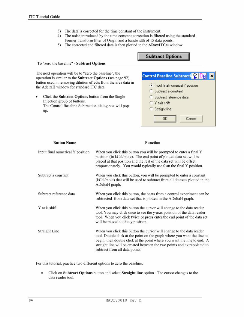
ITC Tutorial Guide
84 MAU130010 Rev D
3) The data is corrected for the time constant of the instrument. 4) The noise introduced by the time constant correction is filtered using the standard
Fourier transform filter of Origin and a bandwidth of 15 data points.. 5) The corrected and filtered data is then plotted in the ARawITCsi window.
To "zero the baseline" - Subtract Options
The next operation will be to "zero the baseline", the operation is similar to the Subtract Options (see page 92) button used in removing dilution effects from the area data in the AdeltaH window for standard ITC data. • Click the Subtract Options button from the Single
Injection group of buttons. The Control Baseline Subtraction dialog box will pop up.
Button Name Function
Input final numerical Y position When you click this button you will be prompted to enter a final Y position (in kCal/mole). The end point of plotted data set will be placed at that position and the rest of the data set will be offset proportionately. You would typically use 0 an the final Y position.
Subtract a constant When you click this button, you will be prompted to enter a constant (kCal/mole) that will be used to subtract from all datasets plotted in the ADeltaH graph.
Subtract reference data When you click this button, the heats from a control experiment can be subtracted from data set that is plotted in the ADeltaH graph.
Y axis shift When you click this button the cursor will change to the data reader tool. You may click once to see the y-axis position of the data reader tool. When you click twice or press enter the end point of the data set will be moved to that y position.
Straight Line When you click this button the cursor will change to the data reader tool. Double click at the point on the graph where you want the line to begin, then double click at the point where you want the line to end. A straight line will be created between the two points and extrapolated to subtract from all data points.
For this tutorial, practice two different options to zero the baseline.
• Click on Subtract Options button and select Straight line option. The cursor changes to the data reader tool.

Lesson 7: Advanced Curve Fitting
MAU130010 Rev D 85
• Double click the data reader tool on the near the end of the curve (about 30 minutes) and then double click the data reader tool on the curve at 0 minutes.
• Origin quickly creates a straight line which is extrapolated and subtracted from all data points. Your plot should look like this:
• Now Click on the Read Data button and re-open the OneInj001.sim data file, • Click on Subtract Options button and select Input final numerical Y position option. • Enter 0 in Value window. • Click OK.
Your plot should look like this: Use this data set for subsequent curve fitting. To Remove Bad Data

ITC Tutorial Guide
86 MAU130010 Rev D
Hint: When moving a data marker you may press the space bar to increase the size of the cross-hair
Data at the beginning of the experiment will be distorted by the time constant correction and there may be extraneous data points after the injection was completed. The Remove Bad Data button will simplify the task of excluding these data points from subsequent analysis. At the start of the injection, typical experiments will have a high point (exothermic reaction) or a low point (endothermic reaction). When you select the Remove data before option, you may select either the High Point or Low Point check box, then when you click OK, Origin will search each data set and delete all data before the corresponding High or Low point in the data. The data will then be plotted on the graph with the beginning data removed. Alternatively, you may select the Remove selected range option. When you select this option button and click OK, each data set will be sequentially plotted on the graph with two data markers displayed on the trace. You may click and drag on a marker to move it to your desired point on the trace, then double click or press enter to set the point. All data between the two markers will be removed from the graph and eliminated from future analysis.. • Click on Remove Bad Data button from Single Injection group. • Select the Remove data before option, then put a check into the Low Point box and click OK.
The graph should look, as shown below
To Normalize Data points

Lesson 7: Advanced Curve Fitting
MAU130010 Rev D 87
• Click the Normalize Data button from the Single Injection group. After clicking the Normalize Data button the concentration continuum will be calculated and the normalized heat will be plotted in a new window, named DeltaH. The data is now in the form of conventional ITC normalized data and may be fit with the methods described in previous Lessons (e.g. Lesson 1, One Set of Sites on page 13). If necessary, you can modify macromolecule and ligand concentrations by clicking Concentration button and entering new values (Page 12).


Lesson 9: Other Useful Details
MAU130010 Rev D 89
Lesson 8: Autosampler Data (Optional Accessory)
The Autosampler is an optional accessory for use with the ITC to allow multiple unattended experiments. The AutoITC Origin module contains curve fitting routines that operate on multiple data files from the autosampler. If you are not familiar with curve fitting of standard ITC data, you should review the previous Lessons of this tutorial, especially Lessons 1, 2, 3 & 4, before starting this lesson.
Launching the ITC Autosampler Data Session
The routines for Auto ITC files are located on a separate window (named ARawITC) from the regular ITC routines.
• To launch the Auto DSC, double-click on the MicroCal LLC Auto ITC icon on the Desk
Top. Or alternatively select Start : Programs : OriginLab : MicroCal LLC Auto ITC
When you start Origin, the program automatically opens the ARawITC graph window.
To input the data
Raw data files from the autosampler are typically a series of data files of the form FamilyName001.ITC, FamilyName002.ITC, FamilyName003.ITC, etc.. The family name may have up 11 alphanumerical characters, VPViewer adds the sequential 3 digit number, therefore there may be a maximum of 14 characters for the filename. To open the file series click on the Read Data… button and the Import Multiple ASCII dialog box will open. Select the Auto ITC Data (*.ITC) as the Files of type, the upper File Name list box will list only the first file of the series (*001.ITC), but when selected all files of the same file name will be read in until the end of the series is reached. Alternatively, you may open individual files or a selection of files similar to the normal ITC method for multiple file input. When you select the Files of type to be ITC Data (*.ITC), then all files with the ‘ITC’ extension will be listed in the upper list box. You may then manually select the files to add to the lower list box and read into Origin.

ITC Tutorial Guide
90 MAU130010 Rev D
To open serial Auto ITC (*001.ITC) files
• Click on the Read Data.. button. The Import Multiple ASCII dialog box opens. Select Auto ITC Data (*.itc) as the Files of type and only ITC files that have 001 before the extension dot will be listed.
• Navigate to the C:\Origin70\Samples folder, and then select itc0523c001.ITC from the Files list.
Please Note: Raw data file names should not begin with a number, nor should they contain any hyphens, periods or spaces.
Note: You may select a default folder for Origin to “Look in” for a data file by selecting File : Set Default Folder… and entering the default path (e.g. for this tutorial you may wish to choose the path to be C:\Origin70\Samples)
• Select itc0523c001.ITC file and click Add File(s).
• Click OK. The itc0523c001 family of files is then read in sequentially (i.e. itc0523c001, itc0523c002…….itc0523c006.). As the files are read in, the following operations take place on each data set. 1) The data is plotted as a line graph in the ARawITC window. 2) Each injection peak is analyzed and a baseline is created 3) The peaks are integrated, and the area (µcal) between the peaks and the baseline is
obtained. 4) The normalized area data is then plotted in the ADeltaH window.

Lesson 9: Other Useful Details
MAU130010 Rev D 91
Note: The Data Control and Model Fitting group of buttons (as shown above) are normally used with the standard ITC data, as described in the previous lessons of this tutorial. These buttons are fully functional on data collected from the AutoITC, but only operate on a single data set.
Auto ITC Buttons
Apart from the buttons associated with the standard ITC, there is a group of buttons labeled AutoITC that perform data manipulations on multiple ITC files. Examples of the use of each button are presented in the following pages. Button Name Function
Subtract Mode When you click this button, the Control Baseline Subtraction dialog box will pop up providing 4 different means to adjust the experimental datasets to minimize the heats of dilution.
One Set of Sites When you select this button, the One Set of Sites fitting model will be applied to all data sets plotted in the AdeltaH graph. The calculated fitting parameters will then be printed in a summary table.
Two Sets of Sites This button will apply the Two Sets of Sites fitting model to all data sets plotted in the active layer, then prints the fitting parameters in a summary table.
Raw Data Window This button provides a quick method to return to the ARawITC window.

ITC Tutorial Guide
92 MAU130010 Rev D
To check and edit concentration values
The concentration values for the cell and syringe are usually entered into the data files when setting up the experiments in VPViewer. You should always check that concentration values are correct for each experiment. Incorrect values will produce erroneous fitting results.
• Select the menu item Window : MicroCal VP-ITC Autosampler Summary Table. The summary table will open and display the concentration values (mM) for the data. If you need to edit the concentration values, enter the value in the appropriate cell, then exit the cell to make the change effective
• Select the menu item Window: ADeltaH to return to the ADeltaH window. To subtract the heats of dilution effect from area data
You may use the Subtract Options button to adjust each integral heat data set, thereby minimizing the effects of the heats of dilution. • Click the Subtract Options button.
The Control Baseline Subtraction dialog box will pop up.

Lesson 9: Other Useful Details
MAU130010 Rev D 93
Button Name Function Subtract reference data When you click this button, the heats from a control experiment can be
subtracted from all data sets that are plotted in the ADeltaH graph. The control experiment must have same or greater number of injections (data points) as any of the plotted data sets.
Subtract a constant When you click this button, you will be prompted to enter a constant (kCal/mole) that will be used to subtract from all datasets plotted in the ADeltaH graph.
Input final numerical Y position When you click this button you will be prompted to enter a final Y position (in kCal/mole). The end point of each plotted data set will be placed at that position and the rest dataset will be offset proportionately.
Y axis shift When you click this button all data sets are moved out of the graph (layer), the cursor will change to the data reader tool, then the first data set will be moved back into the graph. You may click once to see the y-axis position of the data reader tool. When you click twice or press enter the end point of the data set will be moved to that y position, the data set will be removed from the graph and the next file of the series will be plotted in the graph and you may repeated the process for all data sets that were originally plotted in the graph.
Using the One Set of Sites model with multiple data sets
• Click the One Set of Sites button. Each data set that is plotted in the graph will be fitted to the One Set of Sites model and the parameters n (number of sites), K (binding constant), ∆H (enthalpy change ) and ∆S (entropy change) are calculated. These parameters will then be printed in the summary table.
• Select the menu item Window : MicroCal VP-ITC Autosampler Summary Table. The summary table will open display the parameter values.

ITC Tutorial Guide
94 MAU130010 Rev D
Using the Two Sets of Sites model with multiple data sets To fit your data to the Two Sets of Sites model perform the same preliminary operations as described in the previous pages then:
• Click the Two Sets of Sites button. Each data set that is plotted in the graph will be fitted to the Two Sets of Sites model and the eight parameters n1, n2 (number of sites), K1, K2 (binding constants), ∆H1, ∆H2 (enthalpy change ) and ∆S1, ∆S2 (entropy change) are calculated. These parameters will then be printed in the summary table.
To return to the ARawITC window • Click the Raw Data Window button to return to the ARawITC window.

Lesson 9: Other Useful Details
MAU130010 Rev D 95
Single Injection Method with AutoITC
Auto ITC is also capable of carrying out a complete binding experiment using only a single continuous injection as opposed to the normal procedure which requires multiple injections. In this single-injection procedure, only one slow, continuous injection of ligand solution is made from the injection syringe into the macromolecule solution contained in the sample cell. It should be pointed out that the binding parameters obtained from a well designed multiple injection experiment usually have higher degree of accuracy than the single injection experiment. If the sample turnover rate is not a prime concern users should perform the multiple injection experiment for more precise binding parameters. Correction of Raw Data for time constant of the instrument, etc. There are several operations which are automatically performed by Origin when the data file is opened : a) data corrected for the time constant of the instrument. and b) corrected data set is filtered using the standard Fourier transform filter in Origin 7.0 and a bandwidth of 15 data points. The user then a) sets the “zero baseline” from which the experimental data will be subtracted. (page 97-98), and b) exclude distorded or extraneous data points prior to subsequent analysis (page 99).
Creating New Worksheet. The raw data (after time constant correction, Fourier filtering, baseline subtraction, and eliminating inappropriate data) can then be used to form a new worksheet which is modeled after the existing worksheet used with multi-injection binding data.
To create SIM Auto ITC icon on desktop
• Right-click any Origin 7 icon on the desktop • Choose Copy, then right-click mouse on desktop and choose Paste to create copy of Origin 7
icon. • Rename icon: Right-click the copy of the icon, choose Rename, and enter SIM AutoITC.
• Change target of desktop icon to SIM: Right-click SIM AutoITC icon, choose Properties. In
Target window, change final number of target to 9, enter OK.
To input SIM data
Double-click SIM AutoITC icon on desktop. • Click on the Read Data button in the Single Injection group
The Import Multiple ASCII dialog box opens. Select Auto ITC Data (*.sim) as the Files of type and only ITC files that have 001 before the extension dot will be listed.
• Navigate to the C:\Origin70\Samples folder, and then select OneInj001.sim from the Files list.

ITC Tutorial Guide
96 MAU130010 Rev D
Please Note: Raw data file names should not begin with a number, nor should they contain any hyphens, periods or spaces.
• Select OneInj001sim file and click Add File(s). • Click OK.
TheOneInj001 family of files is then read in sequentially. As the files are read in, the following operations take place on each data set. 1) The data is read into a worksheet that is created with the corresponding name and
RAW appended (i.e. OneInjo001.sim is read into a worksheet named OneInj001RAW).
2) The time before the injection starts (60 seconds) is subtracted from the x data so that the injection starts at t=0 and all data points are shifted to the left. Note: The x data before t=0 is removed from the worksheet, but the data is still plotted in the graph for use in baseline subtraction.
3) The data is corrected for the time constant of the instrument. 4) The noise introduced by the time constant correction is filtered using the standard
Fourier transform filter of Origin and a bandwidth of 15 data points.. 5) The corrected and filtered data is then plotted in the ARawITCsi window.

Lesson 9: Other Useful Details
MAU130010 Rev D 97
To "zero the baseline" - Subtract Options
The next operation will be to "zero the baseline", the operation is similar to the Subtract Options (see page 92) button used in removing dilution effects from the area data in the AdeltaH window for standard ITC data. • Click the Subtract Options button from Single
Injection the group of buttons. The Control Baseline Subtraction dialog box will pop up.
(
Button Name Function
Input final numerical Y position When you click this button you will be prompted to enter a final Y position (in kCal/mole). The end point of each plotted data set will be placed at that position and the rest dataset will be offset proportionately. You would typically use 0 an the final Y position.
Subtract a constant When you click this button, you will be prompted to enter a constant (kCal/mole) that will be used to subtract from all datasets plotted in the ADeltaH graph.
Subtract reference data When you click this button, the heats from a control experiment can be subtracted from all data sets that are plotted in the ADeltaH graph.
Y axis shift When you click this button all data sets are moved out of the graph (layer), the cursor will change to the data reader tool, then the first data set will be moved back into the graph. You may click once to see the y-axis position of the data reader tool. When you click twice or press enter the end point of the data set will be moved to that y position, the data set will be removed from the graph and the next file of the series will be plotted in the graph and you may repeated the process for all data sets that were originally plotted in the graph.
Straight Line When you click this button all data sets are moved out of the graph (layer), the cursor will change to the data reader tool, then the first data set will be moved back into the graph. Double click at the point on the graph where you want the line to begin, then double click at the point where you want the line to end. A straight line will be created between the two points and extrapolated to subtract from all data points. The first data set will be removed from the graph and the next file of the series will be plotted in the graph and you may repeated the process for all data sets that were originally plotted in the graph.

ITC Tutorial Guide
98 MAU130010 Rev D
For this tutorial, practice two different options to zero the baseline.
• Click on Subtract Options button and select Straight line option. Data set OneInj001 is the only data set in the active window, and the cursor changes to the data reader tool.
• Double click the data reader tool on the near the end of the curve (about 30 minutes) and double click again on the curve at about 0 minutes.
• Origin quickly creates a straight line which is extrapolated and subtracted from all data points. • Data set OneInj002 is now the only data set in the active window. Repeat above steps for this
data set. • Repeat for remaining data sets.
Your plot should look like this:
• Now Click on the Read Data button and re-open the OneInj001 data file, • Click on Subtract Options button and select Input final numerical Y position option. • Enter 0 in Value window. • Click OK.
Your plot should look like this: Use this data set for subsequent data analysis.

Lesson 9: Other Useful Details
MAU130010 Rev D 99
Hint: When moving a data marker you may press the space bar to increase the size of the cross-hair
To Remove Bad Data
Data at the beginning of the experiment will be distorted by the time constant correction and there may be extraneous data points after the injection was completed. The Remove Bad Data button will simplify the task of excluding these data points from subsequent analysis. At the start of the injection, typical experiments will have a high point (exothermic reaction) or a low point (endothermic reaction). When you select the Remove data before option, you may select either the High Point or Low Point check box, then when you click OK, Origin will search each data set and delete all data before the corresponding High or Low point in the data. The data will then be plotted on the graph with the beginning data removed. Alternatively, you may select the Remove selected range option. When you select this option button and click OK, each data set will be sequentially plotted on the graph with two data markers displayed on the trace. You may click and drag on a marker to move it to your desired point on the trace, then double click or press enter to set the point. All data between the two markers will be removed from the graph and eliminated from future analysis.. • Click on Remove Bad Data button from Single Injection group. • Select the Remove data before option, then put a check into the Low Point box
and click OK.

ITC Tutorial Guide
100 MAU130010 Rev D
To Normalize Data points
• Click the Normalize Data button from the Single Injection group.
After clicking the Normalize Data button the concentration continuum will be calculated and the normalized heat will be plotted in a new window, named DeltaH. The data are now in the form of conventional ITC normalized data and may be fit with the methods described in pages 93 and 94.

Lesson 9: Other Useful Details
MAU130010 Rev D 101
Lesson 9: Other Useful Details
Chi-square (chi^2) Minimization
The aim of the fitting procedure is to find those values of the parameters which best describe the data. The standard way of defining the best fit is to choose the parameters so that the sum of the squares of the deviations of the theoretical curve(s) from the experimental points for a range of independent variables is at a minimum. For the ITC models, where there is no weighting, the theoretical models can be represented by: where: pi = the fitting parameters the expression for χ2 simplifies to :
where: neff = the total number of experimental points used in the fitting p = total number of adjustable parameters yi = experimental data points f(x;p1,p2,p3,…) = fitting function Note: the difference d = neff - p is usually referred to as the number of degrees of freedom. The above equation states that the Chi squared value of the fit is equal to the sum of the squares of the deviations of the theoretical curve(s) from the experimental points divided by the number of degrees of freedom. Since there is no weighting, it can be seen that the calculated values are dependent on the magnitude of the scale and the number of data points. After fitting this value is reported as Chi^2/DoF.
Line Types for Fit Curves
You may select a line type to plot your data or fit curves from the Plot Details dialog box. The Plot Details dialog box is available by double-clicking on the data plot, right-clicking on the data plot and selecting Plot Details from the shortcut menu or selecting the desired data plot from the Data menu data list and selecting Format:Plot.
,...),,;( 321 pppxfy =
( )[ ]∑ −−
= 221
2 ,...,;1 ppxfypn iieffχ

ITC Tutorial Guide
102 MAU130010 Rev D
The Line Group
Select the desired line connection from the associated Connect drop-down list. The line connection type affects interpolation results. The default line type for fit curves is Straight line. The most common method of connecting the fit curve data points are straight, spline or B-spline: Straight: A straight line is displayed between data points. This type of line connection will not give a smooth representation of the fit curve if there are few data points. Spline: This option generates a cubic spline connection. To use the connection, the X values must be discrete and increasing. Furthermore, the number of data points cannot exceed 900 (if the data set exceeds this number, the operation will fail).
Since curvature information is held in memory, the spline resolution remains the same regardless of page magnification. The SplineStep variable in the ORIGIN.INI file controls the spline calculation increment. It is expressed in units of .1 point. This is usually the most satisfactory representation of the fit curve, but may exhibit an excursion from the actual fit curve if there is a sharp corner in the data. B-Spline: The B-spline curve can be described by parametric equations. Unlike spline curves which pass through the original data points, the B-spline curve winds around the original data points without passing through them. Thus this curve may not produce a satisfactory representation of the fit curve. For a complete discussion of the B-spline connection, see the Origin User's Manual
Inserting an Origin graph into Microsoft® Word
There are two ways to include your Origin graph into Word (or other applications), you may import your graph into Word or you may link (share) your graph with Word. When you import your graph, Word will display the graph as an object and it cannot be edited by Origin tools (although it may be resized or reposition in the Word document). When you link (share) your graph, Word displays the graph as an object which can be edited by Origin and updated when the Origin graph changes. Please refer to the Origin manual for more information about Creating a Graphic Presentation.
Importing your graph into Word • Create you graph in Origin and when you are satisfied with its appearance, select
Edit:Copy page.
• Open your Word document and click at the location where you want the graph to be located.
• Select Edit:Paste Special. • Select Origin Graph Object from the As list box.
• Select the Paste radio button.
• Click OK.

Lesson 9: Other Useful Details
MAU130010 Rev D 103
Linking your graph into Word
• You must first create your graph in Origin and then save it as part of an Origin project (*.OPJ).
• Open the saved Origin project (if it is not already opened) that includes the desired graph window.
• Make the desired graph window active, select Edit:Copy Page.
• Open your Word document and click at the location where you want to insert the graph.
• Select Edit:Paste Special.
• Select Origin Graph Object from the As: list box
• Select the Paste Link radio button.
• Click OK.
After your Origin graph is linked to Word you may return to the original Origin graph and make changes to the graph. These changes can be reflected in the Word document by:
• Select Edit:Update Client from the Origin menu (to make immediate changes to the Word document graph).
(Shortcut: You may quickly start Origin and load the linked graph by simply double-clicking on the graph while in Word. Origin will be started with the original document loaded, the changes can be made and by selecting Edit:Update Client, the changes will be transferred to the Word document.)
Calculating a Mean Value for Reference Data
You may quickly calculate a mean value for the area data of any reference (or blank) injections by the following method. For this example we will calculate the mean of the area data of the reference file Febuf10.itc (see Subtracting Reference Data starting on page 34). • From the RawITC window, click on Read Data.. button and open the file
Febuf10.itc (located in the [Origin70][Samples] folder).
• Open the area data worksheet by right-clicking on any data point of the Febuf10.itc data set in the DeltaH window and selecting Plot Details : Worksheet from the menu.
• Select the NDH column by clicking on the column heading.
All the cells of the column should be highlighted. • Click on the Statistics on Column(s) button. (Note: If you do not see the button
while the worksheet is open ; Select View:Toolbars then select the Worksheet check box.)
A new worksheet will appear with the mean, standard deviation, standard error of the mean, the sum of the data and the number of data points of the NDH dataset column.

ITC Tutorial Guide
104 MAU130010 Rev D
This page was intentionally left blank

Appendix: Equations Used for Fitting ITC Data
MAU130010 Rev D 105
Appendix: Equations Used for Fitting ITC Data
I. General Considerations
It will be assumed throughout that the macromolecule M is in the cell at an initial bulk concentration otM
(moles/liter) before the first injection, and the ligand X to be injected is initially at zero concentration in the cell. The working volume (cross-hatched area below) of the lollipop-shaped cell is Vo, the size of the ith injection is ∆Vi and the total liquid which has been injected at any point during the experiment, ∆V, is simply the sum of the individual ∆Vi for all injections.
At the beginning of an experiment, both the cell and the long communication tube are filled with macromolecule solution, but it is only that contained within Vo that is sensed calorimetricallly, Because of the total-fill nature of the cell each injection acts to drive liquid out of the working volume and up into the inactive tube as shown by the darkened portion representing ∆V. Thus, the concentration of macromolecule in V changes a small amount with each injection since the total number of moles of macromolecule initially in V (i.e. o
tM times Vo) at the beginning of the experiment is later distributed in a larger volume, Vo + ∆V. Since the average bulk concentration of macromolecule in ∆V is the mean of the beginning concentration Mt
o and the present concentration Mt in the active volume, then conservation of mass requires that
( )M V M V M M Vto
o t o t to= + +
12
∆ (1)
so that
M M
VVV
V
t to o
o
=−
+
12
12
∆
∆ (2)
Using similar reasoning, it is easily shown that the actual bulk concentration of ligand in Vo, Xt, is related to the hypothetical bulk concentration X t
o (assuming that all of the injected ligand remained in Vo) as follows:
VXVXVX totoot ∆+=
21
(3)
oV
V∆

ITC Tutorial Guide
106 MAU130010 Rev D
X X VVt t
o
o
= −
1
2∆
(4)
q The above expressions for Mt and Xt are used by Origin to correct for displaced volume effects which occur with each injection.
II. Single Set of Identical Sites
In the following equations,
K = Binding constant; n = # of sites; Vo = active cell volume; Mt and [M] are bulk and free concentration of macromolecule in Vo; Xt and [X] are bulk and free concentration of ligand, and Θ = fraction of sites occupied by ligand X.
( )[ ]
KX
=−ΘΘ1
(5)
[ ]X X n Mt t= + Θ (6) Combining equations (5) and (6) above gives
Θ Θ2 1 1 0− + +
+ =
XnM nKM
XnM
t
t t
t
t
(7)
The total heat content Q of the solution contained in Vo (determined relative to zero for the unliganded species) at fractional saturation Θ is
Q n M HVt o= Θ ∆ (8)
where ∆H is the molar heat of ligand binding. Solving the quadratic equation (7) for Θ and then substituting this into eq. (8) gives
( )Q
nM HVt o XnM nKM
XnM nKM
XnM
t
t t
t
t t
t
t= + + − + + −
∆2
1 11 12 4
(9)
The value of Q above can be calculated (for any designated values of n, K, and ∆H) at the end of the ith injection and designated Q(i). The parameter of interest for comparison with experiment, however, is the change in heat content from the completion of the i-1 injection to completion of the i injection. The expression for Q in eq. (9) only applies to the liquid contained in volume Vo. Therefore, after completing an injection, it is obvious that a correction must be made for displaced volume (i.e., ∆Vi = injection volume) since some of the liquid in Vo after the i-1 injection will no longer be in Vo after the ith injection, even though it will contribute to the heat effect (assuming the kinetics of reaction and mixing are fast) before it passes out of the working volume Vo. The liquid in the displaced volume contributes about 50%

Appendix: Equations Used for Fitting ITC Data
MAU130010 Rev D 107
as much heat effect as an equivalent volume remaining in Vo1 The correct expression then for heat released,
∆Q(i), from the ith injection is
∆Q i Q idVV
Q i Q i Q ii
o
( ) ( ) ( ) ( ) ( )= ++ −
− −
12
1 (10)
The process of fitting experimental data then involves 1) initial guesses (which most often can be made accurately enough by Origin) of n, K, and ∆H; 2) calculation of ∆Q(i) for each injection and comparison of these values with the measured heat for the corresponding experimental injection; 3) improvement in the initial values of n, K, and ∆H by standard Marquardt methods; and 4) iteration of the above procedure until no further significant improvement in fit occurs with continued iteration.
III. Two Sets of Independent Sites
Using the same definition of symbols as above for set 1 and set 2, we have
( )[ ]
KX1
1
11=
−ΘΘ
( )[ ]XK
2
22 1 Θ−
Θ= (11)
[ ] ( )X X M n nt t= + +1 1 2 2Θ Θ (12) Solving equation (11) for Θ 1 and Θ 2 and then substituting into equation (12) gives
[ ] [ ][ ]
[ ][ ]
X Xn M X K
X Kn M X K
X Ktt t= +
++
+1 1
1
2 2
21 1 (13)
Clearing equation (13) of fractions and collecting like terms leads to a cubic equation of the form
[ ] [ ] [ ]X p X q X r3 2 0+ + + = (14)
where
( )pK K
n n M Xt t= + + + −1 1
1 21 2
qnK
nK
MK K
XK Kt t= +
− +
+1
2
2
1 1 2 1 2
1 1 1
rX
K Kt=
−
1 2
(15)
1 The first infinitesimal volume element in the i injection contributes no heat effect since it has already equilibrated at existing concentrations after the i-1 injection. The last volume element of an injection contributes heat effects equal to the liquid remaining in Vo since its concentrations are equivalent to those in Vo after the i injection. Assuming linearity over the small ∆Vi volume increment, then the liquid in the displaced volume is only half as effective in producing heat relative to the liquid in Vo).

ITC Tutorial Guide
108 MAU130010 Rev D
Equations 14 and 15 can be solved for [X] either in closed form or (as done in Origin) numerically by using Newton’s Method if parameters n1, n2, K1, and K2 are assigned. Both Θ1 and Θ2 may then be obtained from equation 11 above.
As discussed earlier in section II, the heat content after any injection i is equal to
( )Q M V n H n Ht o= +1 1 1 2 2 2Θ ∆ Θ ∆ (16)
After a similar correction for displaced volume, the pertinent calculated heat effect for the i injection is
∆Q i Q idVV
Q i Q i Q ii
o
( ) ( ) ( ) ( ) ( )= ++ −
− −
12
1 (17)
which may be used in the Marquardt algorithm to obtain best values for the six fitting parameters.
IV. Sequential Binding Sites
For sequential binding, the binding constants K1, K2, .....Kn must be defined relative to the progress of saturation, so that
[ ][ ][ ]XM
MXK =1 [ ][ ][ ]
KMX
MX X22=
[ ][ ][ ]
KMX
MX X33
2
= (18)
In the sequential model, there is no distinction as to which sites are saturated, but only as to the total number of sites that are saturated. If the sites are identical, then there is a statistical degeneracy associated with the sequential saturation since the first ligand to bind has more empty sites of the same kind to choose from than does the second ligand, etc. For identical interacting sites then, we can distinguish between the phenomenological binding constants Ki (defined by eq (18)) and the intrinsic binding constants Ki
o where the effect of degeneracies has been removed. The relationship between the two binding constants is given by:
oii K
iinK 1+−
= (19)
All calculations given below, as well as parameters reported from curve-fitting, are in terms of Ki values but the operator may convert to Ki
o values, if desired, using eq (19). Since concentrations of all liganded species [MLi] can be easily expressed in terms of the concentration of the non-liganded species, [M], then the fraction of total macromolecule having i bound ligands, Fi, is simply

Appendix: Equations Used for Fitting ITC Data
MAU130010 Rev D 109
FPo =1
[ ]F
K XP1
1=
(20)
[ ]F
K K XP2
1 22
=
[ ]F
K K K XPn
nn
= 1 2 ....
where
P K X K K X K K K Xnn= + + + +1 1 1 2
21 2[ ] [ ] .... .... [ ]
(21)
X X M iFt t ii
n
= +=∑[ ]
1
Once n and values of fitting parameters K1 through Kn are assigned, then equations (20) - (21) may be solved for [X] by numerical methods (the Bisection method is used). After [X] is known, all Fi may be calculated from equation (20) and the heat content after the ith injection is determined from
[ ] [ ]( )nnot HHHHFHHFHFVMQ ∆++∆+∆+∆++∆+∆+∆= ........... 32121211 (22)
And, as before,
∆Q i Q idVV
Q i Q i Q ii
o
( ) ( ) ( ) ( ) ( )= ++ −
− −
12
1 (23)
Which then leads into the Marquardt minimization routine.

ITC Tutorial Guide
110 MAU130010 Rev D
V. Enzyme/substrate/inhibitor Assay
Assaying enzymes, inhibitors or substrates by calorimetric activity has the major advantage that it works well for any enzyme/substrate/inhibitor system with no prior chemical modification of any participants in the reaction. The rate Rt of the substrate decomposition reaction is directly proportional to the power output in the calorimeter cell, i.e.,
0HV
PRt ∆= (24)
where P is the power generated by the reaction, ∆H is the heat of decomposition of the substrate, and Vo is the cell volume. The units of Rt will be moles/l/sec if P is expressed in µcal/sec, ∆H in µcal per mole of substrate, and Vo in liters, for example.
If Michaelis-Menten kinetics are assumed then the experimental values for the rate Rt can be expressed as
++
=
IMt
tcatcatt
KIKS
SEkR
][1][
][][ (25)
where kcat is the catalytic rate constant for substrate decomposition, KM is the Michaelis constant, [E]tot is the total enzyme concentration, and [S]t is the instantaneous concentration of substrate. The equation as written is valid both in the absence or presence of a competitive inhibitor at concentration [I] and with inhibition constant KI.
The use of equation (25) assumes no effects from product inhibition. This assumption has been discussed by Todd and Gomez (Todd, M. J. & Gomez, J. (2001) Analytical Biochemistry 296, 179-187.) and found to be quantitative in many cases. In those cases where product inhibition is significant, then equation (25) can only be used to express initial rates of reaction prior to accumulation of product.
Todd and Gomez discussed in some detail the two methods by which assays can be carried out in a titration calorimeter, and these are summarized below.
Method 1: Single injection. Using this approach, the reaction is initiated by injecting enzyme solution from the syringe into the sample cell containing substrate solution, or vice versa. If desired, a competitive inhibitor may also be included in one solution or the other. The reaction is allowed to go to completion in the calorimeter cell, and the power P is recorded as a function of time t.
Integration of the excess power P associated with the reaction enables ∆H to be determined, i.e.,
00
0
][ VS
PdtH
t=
∞
∫=∆ (26)

Appendix: Equations Used for Fitting ITC Data
MAU130010 Rev D 111
where [S]t=0 is the starting substrate concentration. Knowing ∆H, the substrate concentration can be determined as a function of time from the equation:
00][][HV
PdtSS
t
ott ∆−=∫
= (27)
After obtaining the time-dependent rate from equation (24), then these data can be equated to the Michaelis expression in equation (25) to provide the final equation to be fit by non-linear least squares. In the absence of inhibitor, kcat and KM are used as variable parameters during iterative fitting. In the presence of inhibitor I, it is best to enter previously determined values of kcat and KM and use KI as the only variable fitting parameter.
Method 2: Multiple injections. In this method, multiple injections of substrate solution from the syringe are made into the reaction cell containing enzyme solution (with or without inhibitor). After each injection, a sufficient time is allowed for the instrument to equilibrate at the new power level resulting from the increased substrate concentration. Measurements are carried out quickly enough however so that little hydrolysis of substrate takes place relative to the total substrate contained in the cell. That is, [S]t is calculated directly from the total added substrate assuming no significant hydrolysis.
Equations (24)-(25) are still valid for Method 2, except that Rt and [S]t now correspond to discrete values of the rate and substrate concentration after each injection, rather than time-dependent values. To determine ∆H from equation (26), it is necessary to carry out another single-injection experiment where hydrolysis is allowed to go to completion. Having done this, then discrete values of Rt at different [S]t are calculated, so that equation (25) can then be fit to obtain best values of kcat and KM (in the absence of inhibitor). In the presence of a competitive inhibitor, data are also fit to equation (25) but using kcat and KM as fixed (results obtained from previous experiment with no inhibitor present) and treating KI as the only fitting parameter.
VI. Dimer Dissociation Model
A protein molecule P may associate at high concentrations to form a dimer. The dilution of this concentrated protein solution by injection into the calorimeter cell containing buffer can then result in some heat effects from dissociation
PPdiscH
22 ⇔∆
( )( )2
2
PPK =
where (P) and (P2) are the concentrations of monomer and dimer and where ∆Hdisc is the heat of dissociation of the dimer. It is assumed in this model that the stoichiometry is well-defined, i.e., no aggregates with stoichiometry higher than 2 are present. By measuring heats for a series of injections it is then possible, using curve-fitting, to determine the dissociation constant K, and heat of dissociation.
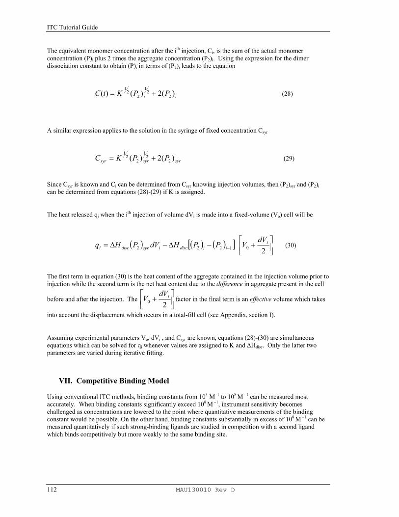
ITC Tutorial Guide
112 MAU130010 Rev D
The equivalent monomer concentration after the ith injection, Ci, is the sum of the actual monomer concentration (P)i plus 2 times the aggregate concentration (P2)i. Using the expression for the dimer dissociation constant to obtain (P)i in terms of (P2)i leads to the equation
ii PPKiC )(2)()( 22
1
22
1+= (28)
A similar expression applies to the solution in the syringe of fixed concentration Csyr
syrsyrsyr PPKC )(2)( 22
1
22
1+= (29)
Since Csyr is known and Ci can be determined from Csyr knowing injection volumes, then (P2)syr and (P2)i can be determined from equations (28)-(29) if K is assigned.
The heat released qi when the ith injection of volume dVi is made into a fixed-volume (Vo) cell will be
( ) ( ) ( )[ ]
+−∆−∆= − 201222
iiidiscisyrdisci
dVVPPHdVPHq (30)
The first term in equation (30) is the heat content of the aggregate contained in the injection volume prior to injection while the second term is the net heat content due to the difference in aggregate present in the cell
before and after the injection. The
+
20idV
V factor in the final term is an effective volume which takes
into account the displacement which occurs in a total-fill cell (see Appendix, section I).
Assuming experimental parameters Vo, dVi , and Csyr are known, equations (28)-(30) are simultaneous equations which can be solved for qi whenever values are assigned to K and ∆Hdisc. Only the latter two parameters are varied during iterative fitting.
VII. Competitive Binding Model
Using conventional ITC methods, binding constants from 103 M–1 to 108 M –1 can be measured most accurately. When binding constants significantly exceed 108 M –1, instrument sensitivity becomes challenged as concentrations are lowered to the point where quantitative measurements of the binding constant would be possible. On the other hand, binding constants substantially in excess of 108 M –1 can be measured quantitatively if such strong-binding ligands are studied in competition with a second ligand which binds competitively but more weakly to the same binding site.

Appendix: Equations Used for Fitting ITC Data
MAU130010 Rev D 113
Competitive binding studies are carried out using the strong-binding ligand A as the injectant, with the solution in the cell containing the second competitive ligand B as well as the binding protein P (or other target molecule). This system then has two equilibria which are displaced with each injection, i.e.,
]][[][K
]][[][K
B
A
BPPBPBPB
APPAPAPA
B
A
H
H
=⇔+
=⇔+
∆
∆
The value of KB and ∆HB for the competing ligand are first measured in a conventional ITC experiment, and these parameter values are entered as known parameters when determining KA from results of the competition experiment. For the competition experiment, the total concentration of competing ligand, [B]tot, should be selected such that
1-85 M 1010][""
−≅totB
A
BKK
where “KA” is the estimated value of KA.
The detailed equations used in the fitting model for competitive binding are found in a paper by Sigurskjold (Sigurskjold, B. W. (2000) Analytical Biochemistry 277, 260-266.). MicroCal would like to thank Dr. Sigurskjold for providing this fitting routine.
VIII. Single Injection Method
Creating New Worksheet. The raw data (after time constant correction, Fourier filtering, baseline subtraction, and eliminating inappropriate data) are used to form a new worksheet which is modeled after the existing worksheet used with multi-injection binding data.
1) Input Parameters. In addition to the raw data parameters (∆P (ucal/sec) from the Y axis and time t
(sec) from the X axis of the corrected raw data, the known parameters are the injection rate R (µl/sec, stored in header), total delivery volume Vinj (ul, stored in header), active cell volume Vcell (ml), the initial macromole concentration in the cell Mo (mM) before any dilution, the dilution factor dM for the macromolecule solution resulting from autosampler loading, the initial ligand concentration in the syringe Xo before any dilution, the dilution factor dX for the ligand concentration resulting from loading. The approximate values are 0.95 for dM and 0.91 for dX, and the values will be independent of the instrument which is used in the experiment.
2) Point numbering. In the existing Origin worksheet for multiple injections, the rows are numbered 1,2,3, …. according to the injection number. In the worksheet for single injection experiments, the numbering corresponds to the data point number. The data points will be spaced at one for each filter period (2 sec).

ITC Tutorial Guide
114 MAU130010 Rev D
3) DH and time t columns. The DH column corresponds to the column of the same name in the existing Origin ITC worksheet while the time t column is one which doesn’t exist in the existing worksheet and must be added. The DH and time t columns should be filled with the data points from the above data set (after TC correction, FT smoothing, control subtraction, and data trimming). DH is the Y axis value ∆P (ucal/sec) and time t (sec) is the corresponding X axis value.
4) INJV column. All entries into this column should be identical and equal to the injection rate R (ul/sec) times the filter time (2 sec).
5) Xt column.
−
=
cellcell
Xo
t 2000VRt1
1000VRtdX
X
6) Mt column.
+
−=
cell
cellM
0t
2000Vrt1
2000Vrt1
dMM
7) XMt column. t
tt M
XXM =
Note: Indexing for Xt, Mt, and INJV refer to values before the ith injection, while DH, XMt, NDH refer to indexing after the ith injection (the new column time t is also indexed after the ith injection).

Index
MAU130010 Rev D 115
Index
A
Aborting the NLSF Session, 58 Active data set, 33, 39 Active data set icon, 33 Adjust integration session. see Integration details Area data. see also Subtracting reference (buffer)
data deleting, 36 opening multiple runs, 29–31 plotting in DeltaH window, 37 saving, 12
ASCII data transfer. see Exporting ASCII data; Importing Worksheet data
Auto ITC Baseline command, 10 Available Data list
in Layer Control dialog box, 31, 32, 37, 41 in Math dialog box, 38, 40 in Subtract Reference Data dialog box, 34
B
Baseline and Auto ITC Baseline command, 10 creating automatically, 10 modify in adjust integration session, 22–24
Binding equations Competitive, 102–3 Dimer Dissociation, 101–2 Enzyme Assay, 100–101 general considerations, 95–96 Sequential Binding Sites, 98–99 SingleSet of Identical Sites, 96–97 Two Sets of Sites, 97–98
Blank injections. See Subtracting reference data
C
Chi-Sqr button, 57, 64, 80, 81, 91 Competitive binding, 79 Control Parameters dialog box, 59–60 Copy and paste worksheet data, 45–46 Copy command, 45 Curve fitting
Competitive binding, 79 Dimer Dissociation, 75–77 invoking one of the three fitting models, 13 line types, 91–92 Nonlinear Least Squares Fitting Session, 14 One Set of Sites, 13–14 Sequential Binding Sites
fitting procedure, 63–66 Two Sets of Sites, 55–58
with ligand in cell and macromolecule in
syringe, 63 Custom disk
installing, 3–4
D
Data deleting, 36 Importing, 7
Data markers and setting integration range, 24
Data Reader tool, 38 Data set. see also ITC data
active, 39 deleting, 36 mean value, 93 naming, 44 naming conventions, 11–12, 43–44 set as active, 33
Data, deleting points, 27 Deconvolution. see Curve fitting Deleting bad data, 27 DeltaH plot window. see templates Derivative Delta Group, 60 Dimer Dissociation, 77
equations, 101–2 Draft view mode, 7, 21
E
Enzyme Assay, 66–75 equations, 101 Method 1) Substrate Only, 66–70 Method 1) Substrate Plus Inhibitor, 71 Method 2) Substrate Only, 72–74 Method 2) Substrate Plus Inhibitor, 74–75
Exiting Origin, 20
F
Final figure, 17–19 Fitting Function dialog box, 13. see also Curve
fitting Fitting parameters
and Sequential Binding Sites, 63–66, 98–99 and the single set of sites model, 13–14, 96–97 and the two sets of sites model, 55–58, 97–98 general considerations, 96 text box, 14 using macromolecule concentration, 82

ITC Tutorial Guide
116 MAU130010 Rev D
I
Importing data, 7 Importing Worksheet Data, 48 Initialization parameters, 55–58 Installing
Custom Disk, 3–4 Origin, 3
Integrate injection peaks in routine data analysis, 10 Integrate on All Peaks command, 10, 25 single peak, 24
Integration details and modifying baseline, 22–24 defined, 21 To adjust the integration range, 24, 23–25
ITC data. see also Subtracting reference (buffer) data; Area data; Routine ITC data analysis and opening multiple area data runs, 37 and subtracting reference (buffer) data from
reaction heat data, 29, 36–42 data sets created in routine data analysis, 11–
12, 43–44 opening multiple area data runs, 29–31 plotting in DeltaH window, 37
ITCFinal plot window. see Templates Iterations
Max. Number of Iterations, 60
L
Layer Contents list, 31, 32, 37, 41 Layer Control dialog box, 31, 32, 37, 41 Layer icon
double-clicking on, 31, 37, 41 Line types for fit curves, 91–92 Linear Regression command, 39
M
Math dialog box using to subtract reference data, 38–39, 40
Mean value of a data set, 93
Menu Levels, 5
N
Naming a data set, 11–12, 43–44
O
Opening and Analyzing Previous Versions of Origin (*.ORG) Documents, 7
P
Page view mode, 6, 21 Paste command, 46
Plot command, 44, 46 Plot Details dialog box, 18, 25, 36, 44, 91 Plot window templates. see Templates Plotting data. see Area data; ITC data; Raw ITC
data files; Routine ITC data analysis Print view mode, 6 Project
opening, 21, 29, 36, 43, 66, 71, 72, 74, 75, 77 saving, 20
R
Raw ITC data files, opening, 9–10, 37, 43 RawITC plot window. see Templates Reaction heat, subtracting reference from. see
ITC data; Subtracting reference (buffer) data Read Data button, 7, 10, 49, 79 Reference data. See Subtracting reference data Registering with OriginLab, 5 Routine ITC data analysis. see also ITC data
and integrating injection peaks, 10 and opening raw data files, 9–10, 37, 43
S
Save area data, 12 Sequential Binding Sites, 63–66
binding equations, 98–99 multiple ligands to transition metal ions, 65 non-identical sites, 65–66
Significant digits, 60 Simple Math command, 38–39, 40 Simulating Curves, 79–81 Starting Origin, 5 Subtract Reference Data button, 34 Subtracting reference (buffer) data. see also ITC
data and calculating mean value for, 93 and injection time spacing, 36, 41–42 and opening multiple runs, 29–33 subtracting a constant, 38–39 subtracting a straight line, 39–40 with a different number of injections than
reaction data, 36–41 System requirements for Origin, 3
T
Templates defined, 49 DeltaH, 18, 21, 52 ITCFinal, and creating a final figure for
publication, 17–19 modifying and saving, 49–52 units used to display data in, 53–54
Text annotations formatting, 15–16

Index
MAU130010 Rev D 117
repositioning, 15 Time Constant, 69 Tolerance Text Box, 59 Two Sets of Sites
fitting equations, 97–98 fitting procedure, 55–58
U
Units used in default templates, 53–54
V
View Mode and available types, 6
W
Weighting Method, 60 Window view mode, 6 Windows
Restore button, 6, 9 set as active, 46
Worksheet copy and paste worksheet data, 45–46


![Saizen [somatropin (rDNA origin) for injection] For ... · Saizen® [somatropin (rDNA origin) for injection] For subcutaneous or intramuscular injection DESCRIPTION Saizen® [somatropin](https://img.dokumen.tips/doc/110x75/5b8977fc7f8b9abe1e8db061/saizen-somatropin-rdna-origin-for-injection-for-saizen-somatropin.jpg)


![Nutropin AQ [somatropin (rDNA origin) injection] Nutropin ... · Nutropin®®® [somatropin (rDNA origin) for injection] DESCRIPTION ® ®. ® in ® ® ® ® ®. •• ®](https://img.dokumen.tips/doc/110x75/5b8977fc7f8b9abe1e8db08f/nutropin-aq-somatropin-rdna-origin-injection-nutropin-nutropin.jpg)