Embed Size (px)
Citation preview

1
ISSUES IN TRANSMISSIVITY ESTIMATION
G.N. Newsam
Abstract The dependence of transmissivity estimates on head data is both nonlinear and ill-posed, and so is difficult to analyse and solve. The paper looks at the setting of this problem, in particular in what spaces are the actual data and in what spaces can uniqueness be proven. The paper also looks at the problem of finding a discretization that has at least some of the useful properties found in discretizations of linear ill-posed problems based the singular value decomposition. As definitive answers have not yet been found to the many of the questions raised, the paper is intended to serve more as a platform for further work than as a report on results achieved.
1. Introduc.Hon
Water resource management is shaping up as a major issue for Australian communitles. A
succession of local crises (pollution of beaches and rivers, contaminated drinldng water and
land loss due to salinity) has dragged it into the limelight, and, in particular, has brought home
the need for efficient management of what are quite limited resources [1]. Effective
management requires good quantitative models of reality to resolve the many "What if?"
scenarios that arise when a limited resource is to be distributed among many users. As is so
often the case, the importance of Lhe problem is reflected in the intrinsic interest and difficulty of
the mathematical and numerical analysis needed to get reliable results from these models.
The particular mathematical problems considered here arise out of analysis of a model widely
used in groundwater management: that is the modelling steady state flow in a confined aquifer
as an elliptic p.d.e. The model assumes that the observable variables of piezometric head qi.x)
(i.e. water pressure in the aquifer) and recharge I discharge q(x) of water in to I out of the
aquifer may be reasonably related by a p.d.e. of the fonn:
V • (a(x) Vq>(x)) = q(x) (1)
where a(x) > 0 is the transmissivity of the aquifer and Q is the region containing the aquifer.
Effective management of groundwater requires repeated solution of this equation for rp under
differing recharge regimes in order to explore the resulting changes in groundwater flows and

2
associated phenomena, such as the height of the water table and discharges at the margins of the
aquifer.
Before such exploration can be carried out, however, the transmissivity a must be determined.
Transmissivity essentially reflects the porosity of the aquifer and the ease with which water can
flow through it. However, as the model is only valid on scales greater than the width of the
aquifer, transmissivity is really a bulk property of the aquifer and includes the effects of large
scale features such as cracks or gravel lenses as well as small scale pores. Thus transmissivity
cannot be simply inferred from examination of rock cores from drills; indeed the only way to
get "point" measurements of transmissivity is by what are known as pump tests (see, e.g., [6]
and the references therein), and these are relatively costly to make on a large scale. Therefore
the preferred method for determining transmissivity is to take measurements of recharge and
piezometric head in the aquifer's existing equilibrium, and to use these and (1) to infer a.
This parameter identification problem is, however, an ill-posed inverse problem in that
solutions for a can be arbitrarily sensitive to errors in measurements of ({), or to errors in the
model. Therefore numerical solutions of (1) for a need to be preceded by a fairly rigourous
mathematical analysis in order to ensure that they are reliable in some well-defmed sense. This
note briefly discusses the key issues in such an analysis: existence, uniqueness and stability.
As transmissivity estimation is a difficult and at times frustrating problem, many of the points
raised concern still open problems.
2 • Appropriate mathematical settings for the model
Any rigourous analysis requires a well-defmed setting for the model. Given the discontinuous
nature of some of the variables (e.g. recharge), perhaps the most natural interpretation of (1) for
scenario modelling is that it holds in some weak sense. No boundary conditions were given in
(1) as in practice they are not usually known with confidence, so for convenience we assume
here Dirichlet boundary data with ({J(x) = 0 on aD. (This corresponds to maintaining a fixed
pressure on the boundary, and would be true in practice if, for example, the boundary was a
river). In this case (1) might be recast as:
The theory of elliptic p.d.e.'s in weak form is very well developed; in it the most suitable
spaces for the various functions would be: a E L -(D), ffJ E H~(D) and q E H(/(D).

3
If a is known a priori, this setting is also convenient for numerical analysis; it is easiest to set
up approximation schemes and derive error analyses for them in fmite dimensional subspaces
of Hilbert spaces. If, however, a is to be determined, then it would be more convenient that a
also be in a Hilbert space, e.g. £2(!2) or HJ(D).
In opposition to these considerations is the fact that the data on fP and q available for
identification of a usually consist of water pressures measured in a number of bore holes
scattered over the aquifer, together with flow rates of any pumps sunk into the aqnifer plus a
(usually very rough) estimate of wide area recharge rates into the aquifer from above or below.
Moreover any data on a is usually in the form of pump tests. Thus the data consists of the
measurement sets:
am f a(x) dx pump tests B.£x,.)
(/)n = (/)(xn) bore measurements
{qp O(X-Xp) pumps Qp =
qn(x) background recharge
where B.£x) is the ball of radius e around x. Thus translating error bars on the data set into
error bounds on the functions suggests that the setting for the problem most consistent with the
data is: a E Li(D), t/1 E C(.Q) and that q consist of two components q1 and q2 with q1 E C*(D)
and q2 E Li(D).
Finally, in transmissivity estimation (1) is viewed not as an elliptic p.d.e. for fP but as a first
order p.d.e. for a. The standard theory for such an equation centres on the idea of
characteristics along which the solution behaves like an o.d.e., and this theory essentially
requires piecewise continuity of the variables in order for the characteristics to be well defmed.
As we shall see, this appears to be the only setting in which uniqueness can be easily proven.
3. Existence
We shall not examine the particular question of under what conditions a solution exists for the
transmissivity estimation problem, but shall rather make a general point about the existence
question: in a sense it may usually be reduced to questions of uniqueness or stability. To see
this, consider the general linear problem:
4
'X! = g where '1(: X~ Y (2)
If a solution f to (2) does not exist then g must be in Y but not in the range 'l({X)r;;;;Y. If
'l({X);~;y then there are two possibilities: that 'l({X) is a proper subspace of Y. or that 'l({X)
is dense in y. The first case might well be termed strong non-existence since it implies that
there is data g such that:
inftExll'l<J-gll > e > 0
It immediately follows from this that the kernel of the adjoint operator '1(* : Y* ~ X* is non
empty, and that the equation 'l(*u = v will have multiple solutions. Thus in transmissivity
estimation we could settle the question of strong non-existence of a solution a to V. (a Vq;) = q
by deciding whether the adjoint equation Vcfi. VqJ = 0 has a nontrivial solution 1/J.
The second case can be termed weak non-existence since in this case there exists data g and a
sequence fk such that II'J<lk -gil J, 0 but the sequence fk does not converge in the given norm
for X This is essentially a statement that the problem is unstable; under the given norms for
X and y, 'l( does not have a bounded inverse. If, however, X (9') was enlarged
(diminished) by appropriate re-norming (i.e. the problem was recast in a different setting) then
in the new norms '1( may have a bounded inverse, the problem would be stable and a solution
would always exist. The relationship between the new norms and the old can then be used to
characterize the degree of instability of the problem.
4. Uniqueness
Two general results on uniqueness of solutions to (1) for a have previously appeared. The
first, due to Chicone and Gerlach [2], contains an elegant proof showing that if no characteristic
crosses the aquifer then the solution must be unique. This condition applies in the particular
problem considered here since the boundary essentially defines a closed contour for the head q;,
and a characteristic cannot cross a closed contour twice. Their result requires, however, that qJ
be twice differentiable and does not hold out much promise of being generalized to prove
uniqueness of weak solutions of ( 1 ).
The second, due to the author and Claude Dietrich [3], is based integration by parts, and so
may still hold under weaker conditions than those of Chicone and Gerlach. To see if this is
indeed possible, we look more closely at the result and its proof.

5
Theorem 1. If Vrp is continuously differentiable and vanishes only on a set of measure zero
in D, then ( 1) coupled with the condition rp = 0 on ()Q has a unique solution among all
continuously differentiable functions a.
Proof: It suffices to show that V. (a Vrp) = 0 implies a= 0, and this we shall prove by
contradiction. In particular, assume that a non-zero solution does exist, let A+ = {x : a(x);?: OJ
and let D +=DnA+. Then w.Lo.g. we may assume that a(x) > 0 in some subset of Q + with
nonzero measure (if not we simply work with Q- in what follows). Now consider:
J f V • (a Vcp)
Integrating by parts gives:
J T V • (a Vcp) + fa ()cp cp
an
(3)
()Q +
Since V. (a Vp) = 0, the l.h.s. vanishes. By continuity and the construction of Q + at any
point x E iJQ + either a(x) = 0 or q;(x) = o, so that the boundary integral also vanishes. But by
assumption there is some subset of Q+ with nonzero measure such that a Vrp. Vp is strictly
positive. As the integrand is non-negative over the rest of Q+ it follows that the first term on
the r.h.s. is strictly positive, which establishes the desired contradiction. Q.E.D.
The proof rests on the assumption that the functions fP, V. (a VfP) and the level set Q + are
sufficiently nice to permit integration by parts. It is known [5] that the class of sets for which
the Gauss-Green identity:
f div g A.
where
2
divg "~ - ~dXi i=l
holds for every vector-valued continuously differentiable function g : A. --+ 9\2 are the so-called
Cacciopoli sets. These sets can be characterized by the fact that their associated characteristic
functions are in the space BV(Q), where A cc D and BV(Q) is the space of functions of
bounded variation in . D, i.e. the set of all functions f E L 1 ( Q) for which:
sup { f f div g : gi E Crf£2), IMx)l :f 1} Q
(4)
6
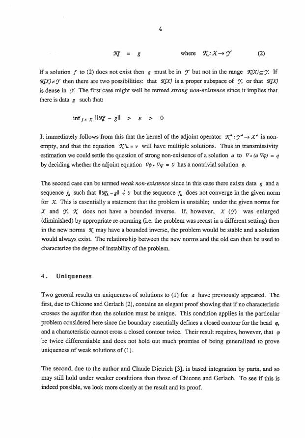
is finite. Moreover it can be shown that if f E BV(.Q) then almost all level sets of f are
Cacciopoli sets.
These results indicate that the minimum requirement on a to ensure that integration by parts is
permissible on the set .Q+ is that a E BV(.Q). Since D c 9!2, the Sobolev inequalities show
that this is roughly comparable to the condition that a E L ~(.a). However, with this restriction
(3) should more properly be rewritten as
L (q>Xa+) V•(a Vcp)
Recognizing cp Xn + as a function of bounded variation, in the worst case it follows from the
definition (4) that integration by parts is valid only if the remainder of the integrand is
continuous, and therefore that a E c 1 (D) and cp E cJmJ.
This shows that striving for the most general level set .a+ does not actually result in a
weakening of the conditions under which the theorem is valid. It may be possible, however, to
get slightly weaker conditions on V. (a V()') by tightening the class of permissible level sets. If
a theory analogous to that of BV(.Q) could be developed by relaxing the class of functions g
appearing in (4) to be, e.g., g, E Hi(D), llg,ll2 = 1 (and so produce a new function space that
was strictly contained in BV(.Q)), then it might be that the existing two conditions (a E BV(D)
and a E C 1(.0), p E C 2(.Q)) could be adjusted simultaneously with the first being strengthened
while the second was relaxed, until ultimately some sort of optimal balance is reached.
Finally, the following example shows that a general uniqueness result for (1) cannot be
established under the weaker conditions: a E L =(D), If> E Hi(D). Let .a= {-1,11 and let ()'(x) =
1-/x/. Now it is simple to show that if a(x) =sgn(x) then
Ja(x)dcpdtf> dx dx dx
-1
5. Stability
0 '<itf>E HJ!:l)
It is clear that a solution a to (1) depends linearly on q but nonlinearly on cp, and furthermore
that a will be stable w.r.t. small perturbations in q (since these are essentially integrated and
so smoothed out in recovering a) but the solution will be unstable w.r.t. small perturbations in
cp (since these are differentiated to give the coefficients in the p.d.e. and are thus amplified). A
rigourous stability analysis confirming this has been given by Richter [8] who showed that,
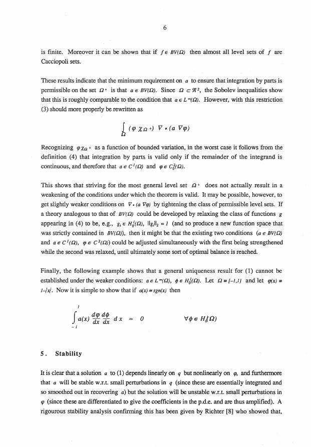
7
under some reasonable conditions needed to ensure uniqueness, given perturbations 7p, if of
the data rp, q (due, e.g., to measurement errors), the induced perturbation in the transmissivity
estimate is bounded above by:
Moreover Falk has given a finite element method for the numerical solution of (1) (again under
certain side conditions necessary to ensure uniqueness) together with an error analysis
consistent with Richter's. In particular, he showed that if a E H r+1Q) and ah is a solution to a
particular discretization of ( 1) using standard finite element spaces and with perturbed data 7p,
then:
(5)
Unfortunately these results do not give much insight into exactly what sort of perturbations in
tp cause instability in a, and thus how to construct a numerical solution that efficiently
approximates only that component of a that is well determined by the model and the data. To
make this point more clearly, consider again the model linear problem (2) with the extra
assumptions that X and 9' are both Hilbert spaces and that '!( is a compact operator. For
simplicity, consider the class of numerical solutions l PO.. got by choosing two N dimensional
subspaces 'U c: X, "v' c: y and then solving the reduced finite dimensional system:
QJ(PfpQ = Qg
where P, Q are the orthogonal projections onto 'll, o/ respectively and g is a perturbation of
the data. After noting that the complete projection of the original system is:
where pc = I -P is the projection onto the complement of 'l1, it follows that
(6)
The terms in Falk's error bound (5) may now be matched with those in (6).
8
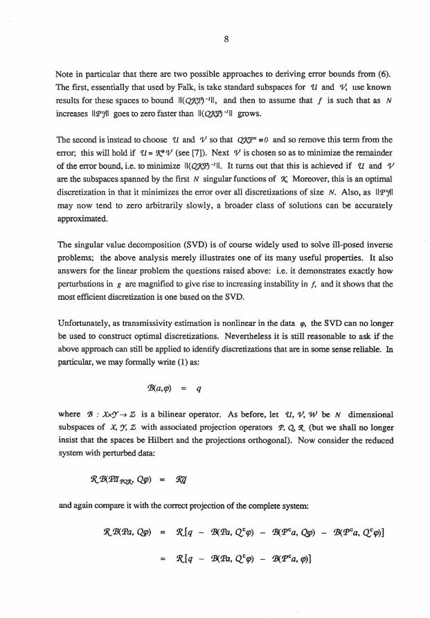
Note in particular that there are two possible approaches to deriving error bounds from (6).
The frrst, essentially that used by Falk, is take standard subspaces for 'U and o/, use known
results for these spaces to bound II(QXP}-1 11, and then to assume that f is such that as N
increases IIP':/11 goes to zero faster than II(Qm') -1 11 grows.
The second is instead to choose 'U and o/ so that QJ(!?• = 0 and so remove this term from the
error; this will hold if 'U = ~o/ (see [7]). Next o/ is chosen so as to minimize the remainder
of the error bound, i.e. to minimize II( Q7(!P) -1 11. It turns out that this is achieved if 'U and o/
are the subspaces spanned by the first N singular functions of ~ Moreover, this is an optimal
discretization in that it minimizes the error over all discretizations of size N. Also, as IIP':tfl
may now tend to zero arbitrarily slowly, a broader class of solutions can be accurately
approximated.
The singular value decomposition (SVD) is of course widely used to solve ill-posed inverse
problems; the above analysis merely illustrates one of its many useful properties. It also
answers for the linear problem the questions raised above: i.e. it demonstrates exactly how
perturbations in g are magnified to give rise to increasing instability in f, and it shows that the
most efficient discretization is one based on the SVD.
Unfortunately, as transmissivity estimation is nonlinear in the data qJ, the SVD can no longer
be used to construct optimal discretizations. Nevertheless it is still reasonable to ask if the
above approach can still be applied to identify discretizations that are in some sense reliable. In
particular, we may formally write (1) as:
f}J(a,lp) q
where '13 : Xx~ ~ Z is a bilinear operator. As before, let 'Zl, o/, 'W be N dimensional
subspaces of X, ?; Z with associated projection operators P, Q, 9{. (but we shall no longer
insist that the spaces be Hilbert and the projections orthogonal). Now consider the reduced
system with perturbed data:
and again compare it with the correct projection of the complete system:
1{.f}J(Pa, QgJ) = 1{.[q
9
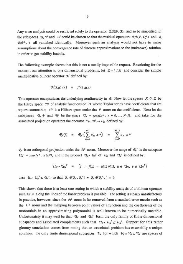
Any error analysis could be restricted solely to the operator !l? .. !B(P·, Q), and so be simplified, if
the subspaces 'll, 'II and 'W could be chosen so that the residual operators 1('13(P., Q'·) and 1<.
'B(Pc·, ·) all vanished identically. Moreover such an analysis would not have to make
assumptions about the convergence rate of discrete approximations to the (unknown) solution
in order to get stability bounds.
The following example shows that this is not a totally impossible request. Restricting for the
moment our attention to one dimensional problems, let Q = [-1,1] and consider the simple
multiplicative bilinear operator :M defined by:
9vf(j,g) (x) = f(x) g(x)
This operator encapsulates the underlying nonlinearity in 'B. Now let the spaces X, ry; Z be
the Hardy space %2 of analytic functions on Q whose Taylor series have coefficients that are
square summable; %2 is a Hilbert space under the [2 norm on the coefficients. Next let the
subspaces 'U, 'II and 'W be the space 'UN= span{xn : n = 0, ... , N-1}, and take for the
associated projection operators the operator PN: :J-P ---!- ·UN defined by:
N-1
L Cn xn
n=O
PN is an orthogonal projection under the :J-{2 norm. Moreover the range of PNc is the subspace
'U/ = span{ X n : n :?: N)' and if the product 'UN. 'UNC of 'UN and 'UNC is defined by:
This shows that there is at least one setting in which a stability analysis of a bilinear operator
such as 'B along the lines of the linear problem is possible. The setting is clearly unsatisfactory
in practice, however, since the %2 norm is far removed from a standard error metric such as
the L 2 norm and the mapping between point values of a function and the coefficients of the
monomials in an approximating polynomial is well known to be numerically unstable.
Unfortunately it may well be that 'UN and 'UN" form the only family of finite dimensional
subspaces and associated complements such that 'UN. 'liNe c 'liNe. Support for this rather
gloomy conclusion comes from noting that an associated problem has essentially a unique
solution: the only finite dimensional subspaces '!IN for which '!IN x o/,v c '!IN are spaces of

10
piecewise constant functions, so that essentially the only orthonormal basis that would generate
a family of such subspaces are the Walsh functions.
6. Conclusion
In conclusion, despite the progress made on transmissivity estimation in the last decade there
are still some important unanswered questions. First, it is still not clear exactly what the correct
mathematical setting for the problem should be. Second, while a weak formulation is the
preferred starting point for numerical solutions, the best results on uniqueness apply only for
continuous functions. This leaves some uncertainty as to the performance of, e.g., finite
element methods on the general problem with discontinuous data. It may be possible to extend
the function spaces on which uniqueness holds by generalizing the idea of bounded variation,
but this is a problem for a different discipline.
Finally, the numerical methods proposed for transmissivity estimation to date have used
standard discretizations and have imposed a priori conditions on the solution in order to bound
the residuals in the associated error analyses. The insight obtainable from these results does not
yet match that available in the theory of linear ill-posed problems: in that theory optimal
discretizations can be defined that separate out exactly that part of the problem for which a
stable solution can be found. A similar approach can at least be formulated for transmissivity
estimation, but a complete solution requires a better understanding of decompositions of
bilinear operators.
References
[1] Murray Basin '88, BMR J. Aust. Geology and Geophysics, 11 (1989).
[2] C. Chicone and J. Gerlach, A note on the identifiability of distributed parameters in elliptic equations, SIAM J. Math. Anal., 18 (1987), 1378-84.
[3] C.R. Dietrich and G.N. Newsam, Sufficient conditions for identifying transmissivity in a confined aquifer, Inverse Problems, 6 (1990), L21-28.
[ 4] R.S. Falk, Error estimates for the numerical identification of a variable coefficient, Math. Comp., 40 (1983), 537-46.
[5] E. Giusti, Minimal Surfaces and Functions of Bounded Variation, Birkhaliser, Boston, 1984.
11
[6] R.B. Guenther and F.A. Mohamed, Well response tests: I. The direct problem, Inverse Problems, 2 (1986), 83-94.
[7] G.N. Newsam, Measures of information in linear ill-posed problems, Technical report no. CMA-R28-84, Centre for Mathematical Analysis, Australian National University, Canberra, 1984.
[8] G.R. Richter, An inverse problem for the steady state diffusion equation, SIAM J. Appl. Math., 41(2) (1981), 210-221.
Information Technology Division, Electronics Research Laboratory, DSTO, P.O. Box 1600, Salisbury, S.A. 5108, Australia.