Embed Size (px)
Citation preview


ISSN 1453 – 7303 “HIDRAULICA” (No. 1/2014) Magazine of Hydraulics, Pneumatics, Tribology, Ecology, Sensorics, Mechatronics
CONTENTS
• EDITORIAL Gabriela MATACHE
5 - 6
• CFD MODEL OF FLOW IN THE OUTLET CHANNEL OF FLOATING CHAMBER Karol STRAČÁR, Jozef KRCHNÁR, Karol PRIKKEL
7 - 13
• BIOMASS COMBINED HEAT AND POWER DFIG CONCEPT CIGRE BENCHMARK NETWORK IMPACT
Curac IOAN, Viorel TRIFA , Bogdan Ionut CRACIUN
14 – 20
• MATERIAL REQUIREMENTS PLANNING, INVENTORY CONTROL SYSTEM IN INDUSTRY
Marin RUSĂNESCU
21 – 25
• THE LUBRICATION IN HIP JOINT Andrea HARINGOVÁ, Karol PRIKKEL, Karol STRAČÁR
26 – 31
• NUMERICAL MODELING OF VISCOUS FLUID FLOW BY SEALING LABYRINTHS Sanda BUDEA, Ştefan SIMIONESCU
32 – 38
• MICROSTRUCTURE AND TRIBOLOGICAL CHARACTERISTICS OF BIOCOMPATIBLE 316 L STAINLESS STEEL
Florina VIOLETA ANGHELINA, Vasile BRATU
39 – 45
• THE FLOW MODELING ON THE CYLINDER VALVE Iulian FLORESCU, Daniela FLORESCU
46 – 49
• INFLUENCE OF CHEMICAL COMPOSITION ON HARDENING PROCESSES, CORRESPONDING FOR ALUMINUM ALLOYS 2024 USED AT HYDRAULIC EQUIPMENT
Vasile BRATU , Florina Violeta ANGHELINA
50 – 57
• AUTOMATION OF A PUMPING STATION FOR LOW POWER APPLICATIONS Laurentiu ALBOTEANU, Gheorghe MANOLEA, Alexandru NOVAC
58 - 64
3

ISSN 1453 – 7303 “HIDRAULICA” (No. 1/2014) Magazine of Hydraulics, Pneumatics, Tribology, Ecology, Sensorics, Mechatronics
MANAGER OF PUBLICATION
- PhD. Eng.Petrin DRUMEA - Hydraulics and Pneumatics Research Institute in Bucharest, Romania
CHIEF EDITOR - PhD.Eng. Gabriela MATACHE - Hydraulics and Pneumatics Research Institute in Bucharest, Romania
EXECUTIVE EDITORS
- Valentin MIROIU - Hydraulics and Pneumatics Research Institute in Bucharest, Romania
- Ana-Maria POPESCU - Hydraulics and Pneumatics Research Institute in Bucharest, Romania
SPECIALIZED REVIEWERS - PhD. Eng. Heinrich THEISSEN – Scientific Director of Institute for Fluid Power Drives and Controls IFAS,
Aachen - Germany
- Prof. PhD. Eng. Henryk CHROSTOWSKI – Wroclaw University of Technology, Poland
- Prof. PhD. Eng. Pavel MACH – Czech Technical University in Prague, Czech Republic
- Prof. PhD. Eng.Alexandru MARIN – POLITEHNICA University of Bucharest, Romania
- Assoc.Prof. PhD. Eng. Constantin RANEA – POLITEHNICA University of Bucharest, Romania
- Lecturer PhD.Eng. Andrei DRUMEA – POLITEHNICA University of Bucharest, Romania
- PhD.Eng. Ion PIRNA - General Manager - National Institute Of Research - Development for Machines and
Installations Designed to Agriculture and Food Industry – INMA, Bucharest- Romania
- PhD.Eng. Gabriela MATACHE - Hydraulics & Pneumatics Research Institute in Bucharest, Romania
- Lecturer PhD.Eng. Lucian MARCU - Technical University of Cluj Napoca, ROMANIA
- PhD.Eng.Corneliu CRISTESCU - Hydraulics & Pneumatics Research Institute in Bucharest, Romania
- Prof.PhD.Eng. Dan OPRUTA - Technical University of Cluj Napoca, ROMANIA
Published by: Hydraulics & Pneumatics Research Institute, Bucharest-Romania Address: 14 Cuţitul de Argint, district 4, Bucharest, cod 040557, ROMANIA Phone: +40 21 336 39 90; +40 21 336 39 91 ; Fax:+40 21 337 30 40 ; E-mail: [email protected] Web: www.ihp.ro with support of: National Professional Association of Hydraulics and Pneumatics in Romania - FLUIDAS E-mail: [email protected] Web: www.fluidas.ro HIDRAULICA Magazine is indexed in the international databases:
HIDRAULICA Magazine is indexed in the Romanian Editorial Platform:
ISSN 1453 – 7303; ISSN – L 1453 – 7303
4

ISSN 1453 – 7303 “HIDRAULICA” (No. 1/2014) Magazine of Hydraulics, Pneumatics, Tribology, Ecology, Sensorics, Mechatronics
EDITORIAL
VREMURI DE SCHIMBARE
Traim vremuri de schimbare. O schimbare haotica si nedefinita prea
bine de cei care vor sa o faca. Punem interesele personale inaintea
intereselor de grup. Promovam nepotismul si mediocrul inaintea
capacitatilor si excelentei. Se cheltuiesc bani si timp cu “experti
europeni” care nu au competente si disponibilitate sa evalueze
obiectiv proiecte depuse cu mult timp in urma. Discrepantele de opinii
si evaluarile pe langa subiecte au distrus sperantele institutelor de
cercetare intr-o evaluare obiectiva a proiectelor depuse la
Parteneriatele 2013.
Dr.ing. Gabriela MATACHE REDACTOR SEF
Punctaje cu diferente de 40 de puncte intre evaluatori arata lipsa de obiectivism a acestora si
faptul ca in realitate nu se doreste o evaluare corecta si concreta a temelor, ci exista numai dorinta
de castig a celor care au “lobby” bine reprezentat in aceste foruri ale cercetarii. Dorim sa
promovam excelenta, dar nu se face nimic in acest sens, iar sprijinul din partea celor care ar trebui
sa-l dea, nu va veni. S-a lansat, nu cu mult timp in urma, cu mult fast programul Orizont 2020. Se
organizeaza de catre toata lumea conferinte, evenimente pe aceasta tema. Sunt adusi experti din
toata lumea sa ne invete cum sa facem si ce sa scriem pentru a castiga proiecte. Dar nimeni nu
spune lucruri concrete, nimeni nu spune ca pentru a realiza aceasta cercetare de “excelenta”
Romania nu are nicio sansa sa castige singura aceste proiecte, ca trebuie depuse impreuna cu tari
UE, astfel incat banii sa se intoarca tot acolo de unde au plecat. Am fost la o astfel de intalnire de
curand, unde un reprezentant al European Research Council ne-a explicat slaba reprezentare a
Romaniei la proiectele FP7. De ce? Probabil si pentru faptul ca in acest Consiliu expertii romani
lipsesc aproape cu…desavarsire. Am spus ‘aproape’ pentru ca sunt cativa care de fapt traiesc si-si
desfasoara activitatea in tari dezvoltate stiintific, ce investesc in oamenii de valoare si-i
promoveaza. Nu cred oare persoanele ce au puterea de a promova cercetarea romaneasca ca
cercetatorii de calitate care traiesc si lucreaza in Romania ar fi bine si ar merita sa fie promovati sa
reprezinte interesele cercetarii romanesti? Cum pot cercetatori “experti” din Diaspora romanesca
sa ne reprezinte pe noi ca tara daca ei sunt rupti de realitatea si nevoile noastre? De unde stiu ei
care sunt temele prioritare si de interes ale Romaniei, daca acolo unde traiesc, muncesc si creaza
nu se confrunta cu greutatile, lipsurile si oportunismul din tara? Poate ca aici ar trebui sa se
gandeasca responsabilii cu cercetarea si sa realizeze ca Romania ca tara nu va evolua decat
rezolvandu-si nevoile si necesitatile actuale.
Pana se va intampla insa ceva, vom continua sa depunem proiecte ce vor fi evaluate de aceeasi
“experti” care cunosc mai bine nevoile tarii noastre.
5

ISSN 1453 – 7303 “HIDRAULICA” (No. 1/2014) Magazine of Hydraulics, Pneumatics, Tribology, Ecology, Sensorics, Mechatronics
EDITORIAL TIMES OF CHANGE
We are going through times of change; a chaotic change, not so well
defined by those who want to do it. We put personal interests above
the interests of the group; promote nepotism and mediocrity prior to
capacity and excellence. They spend time and money with
"European experts" who are not competent and do not have the
willingness to objectively assess projects submitted long ago.
Discrepancies of opinions and off the mark assessments of topics
have destroyed the hopes of research institutes for an objective
assessment of projects submitted under Partnerships 2013.
Ph.D.Eng. Gabriela MATACHE
CHIEF EDITOR
Scores with differences of 40 points between evaluators show their lack of objectivity and the fact
that actually there is not intended a fair and concrete assessment of the themes, but there is only
the desire to win of those who have well represented "lobby" in these bodies of research. We wish
to promote excellence, but nothing is done in this regard, and support from those who are
supposed to give it will not come. It was released, not long ago, with great pomp the programme
Horizon 2020. Everyone organizes conferences, events on the topic. They brought experts from
around the world to teach us how to do and what to write in order to win projects. But no one says
tangible facts; no one says that in order to perform this "excellence" research Romania has no
chance to win these projects by itself, that they must be submitted jointly with EU countries, so that
the money to return back from where they left. I have recently attended such a meeting, where a
representative of the European Research Council explained to us the low representation of
Romania in FP7 projects. Why is it so? Perhaps also because in this Council Romanian experts
are almost completely.... absent. I said ‘almost’ because there are few who actually live and carry
their activity in scientifically developed countries, that invest in valuable people and promote them.
Do not those people who have the power to promote Romanian research believe that it would be
good to promote quality researchers living and working in Romania – and that they deserve to be
promoted - in order for them to represent the interests of Romanian research? How can "expert"
researchers of the Romanian Diaspora represent us as a country, while they are out of touch with
our reality and needs? How do they know which are the topics of interest and priority in Romania, if
there where they live, work and create they do not face the difficulties, shortcomings and
opportunism existent in the country? Maybe this is what the research leaders should think about,
and understand that Romania as a country will evolve only by solving its current requirements and
needs. But until such a thing will happen, we will continue to submit projects, which will be
evaluated by the same "experts" who know better what the needs of our country are.
6

ISSN 1453 – 7303 “HIDRAULICA” (No. 1/2014) Magazine of Hydraulics, Pneumatics, Tribology, Ecology, Sensorics, Mechatronics
CFD MODEL OF FLOW IN THE OUTLET CHANNEL OF FLOATING
CHAMBER
Ing. Karol STRAČÁR*, doc. Ing. Jozef KRCHNÁR*, CSc., doc. Ing. Karol PRIKKEL*, CSc.
*Institute of Chemical and Hydraulic Machines and Equipment, Faculty of Mechanical Engineering, Slovak University of Technology, Nám. slobody 17, 812 31 Bratislava 1 [email protected], [email protected], [email protected]
Abstract: The article deals with the creation of a mathematical model of a floating chamber outlet. The created model should simulate the loading of the segment of a regulatory outlet closure caused by flowing of the fluid around this object. The result should help in designing changes that could help decrease the vibration on segments of the regulatory closure of floating chambers Waterworks Gabčíkovo – Nagymaros.
Keywords: simulation model, CFD, regulatory closures
1. INTRODUCTION
The dynamical component from the flowing fluid will be determined by numerical simulations by means of CFD methods that are a necessary supplement of experiments on a real outlet object. They help us describe the effect of the flow on the regulatory closures segment of the outlet channel of a floating chamber. From this we could determine the loading of the segment without the necessity of time and material consuming and financially demanding measurement. Equally, we get the data about the distribution of examined parameters such as the distribution of pressure, phases in outlet channel or information about the course of the flow velocity in the outlet channel.
CFD methods are used in fluid mechanics where, by means of the numerical methods and solution algorithms, we can analyze problems dealing with the fluid flow. It is possible to obtain information about the interaction of fluids and gases with surfaces, while defining the boundary conditions [6], [7]. The fluid that flows through the outlet channel drains around the regulatory closure segment and influences it by force. The fluid force that acts on the segment is transmitted to a linear hydro-engine. To discover the force effecting on the regulatory closure segment, it is necessary to create a simulation model with a dynamic mesh. Similarly processed also the authors in article [1], where they used the CFD simulations to better understand the complicated flows inside the channel used for the free transfer of fish through the waterworks dam. The possibilities of a CFD solution with dynamic mesh are described in the article [2], where the author describes CFD simulation of a 2D computational analysis of fluid dynamics for a 3-paddle H-Darrieus rotor using nonstructural mesh with a moving model. The description of a flowing field using the CFD models are presented also in the article [4], where the author solved the flow in the area of wave-breaks within the free water surface in a full 3D model.
7

ISSN 1453 – 7303 “HIDRAULICA” (No. 1/2014) Magazine of Hydraulics, Pneumatics, Tribology, Ecology, Sensorics, Mechatronics
FIGURE 1: The forces acting on the regulatory closure segment
The outlet closures allow the entry of water from the floating chamber until an equilibrium of water levels within the lower level is reached in the concerned chamber. The chamber has square dimensions, which means that the setting of the segment is made with a barrier surface of squared shape and 4 x 4m dimensions. The segment is gimbaled, while the movement of the segment can be stopped in any position. All closures have the same structure. Each closure is directed by one linear hydro-engine filled with a pressurized fluid inserted by a hydraulic aggregate [5].
The time of elevation of the regulatory closure segment in the outlet channel of a floating chamber is 120s. The emptying of the floating chamber to a water level suitable for a boat to sail out is approximately 15-20 minutes. However, this is not the time of total water level equilibrium in the floating chamber.
2. THE CREATION OF A SIMULATION MODEL USING THE DYNAMIC MESH
The creation of a dynamic mesh allows us in one simulation to describe the loading rates as well as the pressure and velocity courses during the whole 120 second cycle of the opening of the regulatory closure segment. The example of such a model is in (Fig. 2). It is advantageous to use structural mesh on parts that are sufficiently far away from the regulatory closure segment. However, it is also necessary to use non-structured mesh on areas around the regulatory closure segment that are intended to move. During the designing of the dynamic mesh we made use of the MAP, SUBMAP and PAVE meshing schemes. The final model was composed of 700 000 elements. The input into the simulation model of the outlet channel of the floating chamber is on the left side, the output on the right side (Fig. 2).
8

ISSN 1453 – 7303 “HIDRAULICA” (No. 1/2014) Magazine of Hydraulics, Pneumatics, Tribology, Ecology, Sensorics, Mechatronics
Figure 2: The defined boundary conditions of the model in software Ansys/FLUENT
The input was defined by boundary condition pressure-inlet (1), where the maximum height of the water level was determined and also the height at which the water level decreases during opening. The output was defined by boundary condition pressure-outlet (2), where the height of the water level was set at 9m, which is also the river level. In the upper shaft, similarly to output we set boundary condition pressure-outlet (3), which was defined by the maximum and minimum heights of the water level. The configuration of the height of the water level as input parameter was set by the condition that defined the free level surface in this shaft (the definition of free surface means determination of the borders between fluid and atmosphere). In the numerical simulation, as a flowing media was used water as the primary medium with real values defined for 4°C and as a secondary phase, air. The simulation must be resolved in steps because this method improves the stability as well as the precision of the computation
Moreover, in this case it is necessary to set up in the computational software the parameters of the dynamic mesh, in other words to set up the values for smoothing and re-meshing of the result that is appropriate for the numerical simulation. Apart from the creation of a dynamic mesh, dynamic zones must also be created. In this case a dynamic zone is composed only from the moving regulatory closure segment that is defined as the rigid body. This zone has to have the direction and velocity of the motion also determined, since in our case the segment is moving continuously alongside the circle with velocity 0.035 m/s. In cases of simulation models built up with dynamic mesh, one small disadvantage is the need for a UDF, User Defined Function, subprogram. It is represented by the function determined by the software or environment user. The disadvantage is that this function slows down the computational process in the simulation model, as it influences
9
ISSN 1453 – 7303 “HIDRAULICA” (No. 1/2014) Magazine of Hydraulics, Pneumatics, Tribology, Ecology, Sensorics, Mechatronics
the internal computation system of the own simulation program. Using dynamic mesh through UDF, we define the weight of the regulatory closure segment and the moment point of inertia.
In simulation models where the dynamic mesh is used, we have to first of all find the simulation solution in a stable time mode. In the beginning was created a simple solver scheme, whereas the computation was done in stable time mode with setting up 100 time steps, as previous models were worked out. Later the simulation was set in second and third orders of precision, as is noted in Table 1.
Table 1: Setting up of simulation in the stationary mode in the computational software Ansys/FLUENT
Number of time steps
Pressure - velocity coupling
Pressure Volume fraction Momentum
100 SIMPLE PRESTO! 1st order upwind 1st order upwind
100 Coupled PRESTO! 1st order upwind 1st order upwind
100 Coupled PRESTO! 2nd order upwind 2nd order upwind
100 Coupled PRESTO! 2nd order upwind 3rd order muscl
100 Coupled Body Force Weighted
2nd order upwind 3rd order muscl
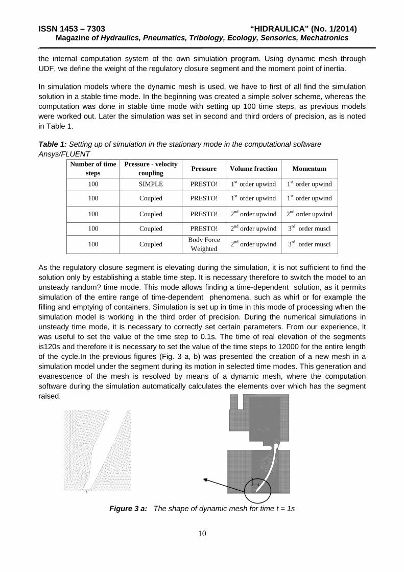
As the regulatory closure segment is elevating during the simulation, it is not sufficient to find the solution only by establishing a stable time step. It is necessary therefore to switch the model to an unsteady random? time mode. This mode allows finding a time-dependent solution, as it permits simulation of the entire range of time-dependent phenomena, such as whirl or for example the filling and emptying of containers. Simulation is set up in time in this mode of processing when the simulation model is working in the third order of precision. During the numerical simulations in unsteady time mode, it is necessary to correctly set certain parameters. From our experience, it was useful to set the value of the time step to 0.1s. The time of real elevation of the segments is120s and therefore it is necessary to set the value of the time steps to 12000 for the entire length of the cycle.In the previous figures (Fig. 3 a, b) was presented the creation of a new mesh in a simulation model under the segment during its motion in selected time modes. This generation and evanescence of the mesh is resolved by means of a dynamic mesh, where the computation software during the simulation automatically calculates the elements over which has the segment raised.
Figure 3 a: The shape of dynamic mesh for time t = 1s
10

ISSN 1453 – 7303 “HIDRAULICA” (No. 1/2014) Magazine of Hydraulics, Pneumatics, Tribology, Ecology, Sensorics, Mechatronics
Figure 3 b: The shape of the dynamic mesh for time t = 15s
During the simulation, in each time step we recorded the forces along the axes „x“and „y“. The values of the forces are represented on the graphs (Fig. 4, Fig. 5). The barrier is connected to a linear hydro-engine, which secures its lifting. One part of the force acting on the barrier is transmitted to the hydro-engine. As the segment is also fixed onto the wall of the outlet channel, one part of the force from the axes „x“ is consumed just at this point and is represented by friction.
Figure 4: The force acting on the segment in direction of x-axis
Figure 5: The force acting on the segment in direction of y-axis
11
ISSN 1453 – 7303 “HIDRAULICA” (No. 1/2014) Magazine of Hydraulics, Pneumatics, Tribology, Ecology, Sensorics, Mechatronics
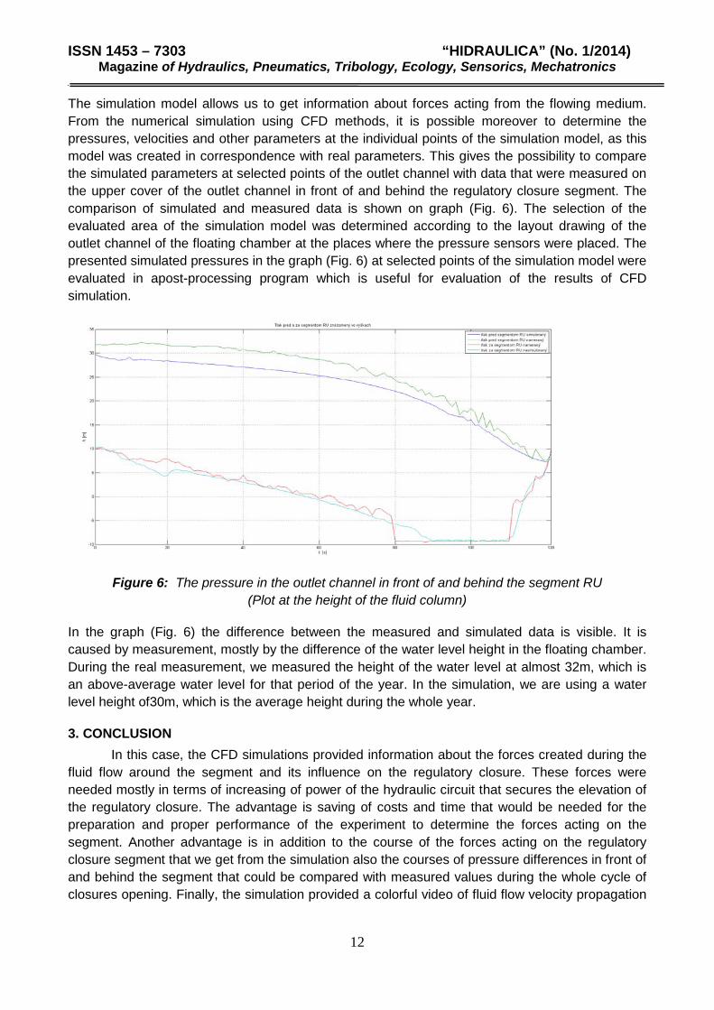
The simulation model allows us to get information about forces acting from the flowing medium. From the numerical simulation using CFD methods, it is possible moreover to determine the pressures, velocities and other parameters at the individual points of the simulation model, as this model was created in correspondence with real parameters. This gives the possibility to compare the simulated parameters at selected points of the outlet channel with data that were measured on the upper cover of the outlet channel in front of and behind the regulatory closure segment. The comparison of simulated and measured data is shown on graph (Fig. 6). The selection of the evaluated area of the simulation model was determined according to the layout drawing of the outlet channel of the floating chamber at the places where the pressure sensors were placed. The presented simulated pressures in the graph (Fig. 6) at selected points of the simulation model were evaluated in apost-processing program which is useful for evaluation of the results of CFD simulation.
Figure 6: The pressure in the outlet channel in front of and behind the segment RU (Plot at the height of the fluid column)
In the graph (Fig. 6) the difference between the measured and simulated data is visible. It is caused by measurement, mostly by the difference of the water level height in the floating chamber. During the real measurement, we measured the height of the water level at almost 32m, which is an above-average water level for that period of the year. In the simulation, we are using a water level height of30m, which is the average height during the whole year.
3. CONCLUSION In this case, the CFD simulations provided information about the forces created during the fluid flow around the segment and its influence on the regulatory closure. These forces were needed mostly in terms of increasing of power of the hydraulic circuit that secures the elevation of the regulatory closure. The advantage is saving of costs and time that would be needed for the preparation and proper performance of the experiment to determine the forces acting on the segment. Another advantage is in addition to the course of the forces acting on the regulatory closure segment that we get from the simulation also the courses of pressure differences in front of and behind the segment that could be compared with measured values during the whole cycle of closures opening. Finally, the simulation provided a colorful video of fluid flow velocity propagation
12

ISSN 1453 – 7303 “HIDRAULICA” (No. 1/2014) Magazine of Hydraulics, Pneumatics, Tribology, Ecology, Sensorics, Mechatronics
alongside the floating chamber outlet channel that could be used in future modifications of this channel.
REFERENCES [1] FERRARI, E. G., POLITANO, M., WEBER, L. Numerical simulation of free surface flows on a fish
bypass. Hydroscience and Engineering, Iowa, Elsevier Ltd., 2008 [2] GUPTA, R., BISWAS, A. Computational fluid dynamics analysis of a twisted three-bladed H-Darrieus
rotor. Journal of renewable and sustainable energy, American Institute of Physics, 2010, ISSN 1941-7012/2010/2(4)/043111/15
[3] PODLESNÝ, J. Diagnostika lineárneho hydrostatického pohonu. STU, Strojnícka fakulta, Bratislava, Dizertačná práca, 2012
[4] YAZDI, J., SARKARDEH, H., AZAMATHULLA, H. MD., GHANI, AB. A. 3D simulation of flow around a single spur dike with free-surface flow. Intl. J. River Basin Management, Vol. 8, No. 1, International Association for Hydro-Environment Engineering and Research, 2010, ISSN 1814-2060 online
[5] Haťová prevádzka a suchý dok plavebnej komory VD Gabčíkovo, STU, Strojnícka fakulta, Bratislava, 2000
[6] Ansys/FLUENT 12.0/12.1 Documentation. Ansys, Inc. 2009 [7] Computational fluid Dynamics. Základná teória CFD, Internet:
http://en.wikipedia.org/wiki/Computational_fluid_dynamics
13

ISSN 1453-7303 “HIDRAULICA” (No. 1/2014) Magazine of Hydraulics, Pneumatics, Tribology, Ecology, Sensorics, Mechatronics
BIOMASS COMBINED HEAT AND POWER DFIG CONCEPT CIGRE
BENCHMARK NETWORK IMPACT
Curac IOAN1, Viorel Trifa ,2 Craciun BOGDAN IONUT3 1 Technical University Of Cluj Napoca, Department of Electrical Machines and Drives, [email protected] 3 Technical University Of Cluj Napoca, Department of Electrical Machines and Drives, [email protected] 2 Aalborg University Department of Energy Technology, [email protected]
Abstract: The following paper has been done in order to analyze the impact of DG penetration in MV CIGRE benchmark network and analyze the medium scale biomass CHP concept impact over the MV grid. Keywords: Biomass, Combined Heat and Power, CIGRE Benchmark Network, DFIG, Distributed Generators
1. Introduction
The market of distributed energy resources (DER) is growing continually and powerfully. Because of this intense growth, the electric power system of centrally located generation, transmission networks and distribution networks is expected to evolve into an infrastructure where small-scale distributed energy resources and loads, connected through local micro grids, are common. Available and reliable methods and techniques are most needed to enable the economic, robust and environmentally responsible integration of DER and to ensure the successful change of the present electric power system. Research and development are active in the whole world in industry, universities and research institutes due to the importance of DER [1]. The power obtained from renewable energy sources has quality problems caused by intermittent and uncontrollable nature of these sources. Among these quality issues there are disturbances in the voltage, oscillations in power flow through the lines, etc. All of them can generate inconveniences. E.g., the voltage disturbances can cause the disconnection of the sensitive equipment and may lead to huge economical loss due to the damaged products. VSCs are largely utilized in most of the DGs (Wind power, Photovoltaic, etc.) and these inverters are very sensitive to voltage disturbances. A disturbance in the voltage can cause disconnection of the inverters from the grid that leads to the loss of energy [2].
2. CIGRE Benchmark Network model
The real network supplies a small town and the surrounding rural area. It has a rated voltage level of 20 kV, being supplied from a 110 kV transformer station, with cable connections for most of the situations, but having some overhead lines sections, too. The network has 30 nodes. This number had to be reduced in order to reduce the size of the network to a required level for DG integration studies but in the same time, maintaining the realistic character [3].
The benchmark network is designed for studying the impact of diverse DG at the medium-voltage level. The list of studies that can be carried out with this benchmark includes the following [3]:
• study of the impact of DG units on the power flow of MV distribution lines; • study of the impact of DG units on the voltage profile in the MV distribution network; • study of energy management systems (DEMS) for DG in the MV distribution network;
14
ISSN 1453-7303 “HIDRAULICA” (No. 1/2014) Magazine of Hydraulics, Pneumatics, Tribology, Ecology, Sensorics, Mechatronics
• study of power quality issues such as harmonics, flicker, frequency variations, and
voltage variations; • study of small signal stability; • study of voltage stability; • study of the impact of MVDC coupling on the power flow of MV distribution lines; • study of the impact of MVDC coupling on the voltage profile in the MV distribution
network; • study of the impact of DG units on transmission capability of the sub-network 1 feeder;
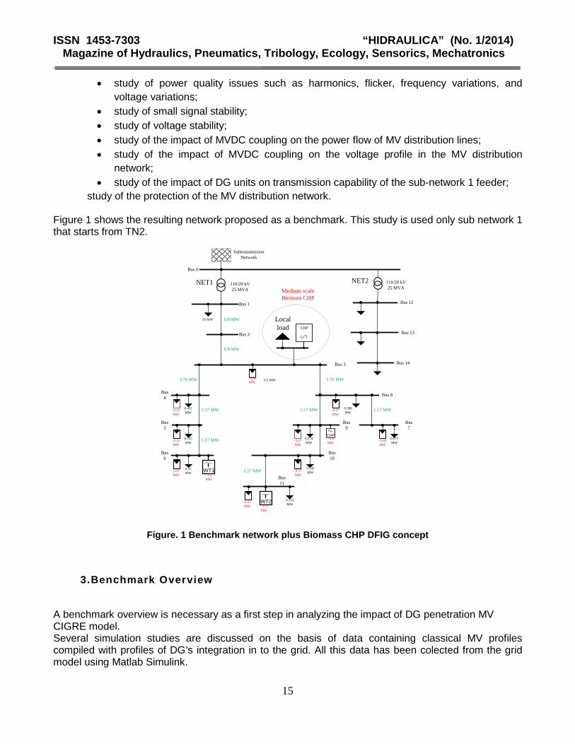
study of the protection of the MV distribution network. Figure 1 shows the resulting network proposed as a benchmark. This study is used only sub network 1 that starts from TN2.
110/20 kV25 MVA
SubtransmissionNetwork
Bus 3
Bus 2
Bus 1
Bus 0
Bus 4
Bus 5
Bus 6
Bus 8
Bus 9
Bus 10
Bus 11
Bus 7
20 MW
0.5 MW
0.432 MW
0.725 MW
0.55 MW
0.588 MW
0.574 MW
0.545 MW
0.331 MW
0.077 MW
- 0.24 MW
- 0.21 MW
- 0.33 MW
- 0.27 MW
- 0.27 MW
- 0.27 MW
- 0.27 MW
- 0.15 MW
- 0.04 MW
8.8 MW
8.8 MW
3.76 MW 3.76 MW
1.57 MW
1.57 MW
1.57 MW
1.57 MW
1.57 MW
Medium scaleBiomass CHP
WT1
WT2- 1.5 MW
- 1.5 MW
- 0.6 MW
CHP
Bus 12
110/20 kV25 MVA
Bus 13
Bus 14
NET2NET1
CHP
Localload
Figure. 1 Benchmark network plus Biomass CHP DFIG concept
3.Benchmark Overview
A benchmark overview is necessary as a first step in analyzing the impact of DG penetration MV CIGRE model. Several simulation studies are discussed on the basis of data containing classical MV profiles compiled with profiles of DG’s integration in to the grid. All this data has been colected from the grid model using Matlab Simulink.
15

ISSN 1453-7303 “HIDRAULICA” (No. 1/2014) Magazine of Hydraulics, Pneumatics, Tribology, Ecology, Sensorics, Mechatronics
The studies were carried out using distribution line as follow:
• industry three-phase dynamic load grid connected on Bus 1 • biomass CHP concept grid connected on Bus 3 • house hold three-phase dynamic load grid connected on Bus 11 • PV power plants grid connected on Bus 1, Bus 3 and Bus 11 • wind turbine grid connected on Bus 11 • internal combustion CHP grid connected on Bus 11
The Three-Phase V-I Measurement block is used to measure instantaneous three-phase voltages and currents in the circuit on each Bus line. The Three-Phase instantaneous active and reactive power is used on transformer terminal strip in oreder to compute the values associated with a periodic set of three phase voltages and current. The following section are presents simulation result of classic medium voltage substation without the integration of DG’s. In the classical representation, the feeders are populated only with loads and the power is delivered in a unidirectional manner. In its initial layout the MV substation provides energy to its end consumers (industrial and residential) and the voltage profile has a descending nature from the MV transformer down to the end consumer located in the last feeders . for this purpose the solution to provide voltage condition was realized by capacitor bank which had the purpose of delivering the needed reactive power to maintain the voltage within the limits.
Figure 2 displays the household consumption profile for 24 hours. As it can be seen the profile follows a normal path of human consumption. It starts ascending at 4:00 AM when people use to wake up and decreases at 9:00 when they are at work. The maximum load is achieved in the afternoon when the characteristic reaches its maximum peak consumption. Figure 3 present the industrial consumption profile for 24 hours. Compared with the household consumption, the industrial load characteristic proves to have its maximum peak in the middle of the day. The figure shows that the profile starts ascending at 5:00 when industry sector starts and decreasing at 16:00.
Figure 2: Household consumption profile over one day
16

ISSN 1453-7303 “HIDRAULICA” (No. 1/2014) Magazine of Hydraulics, Pneumatics, Tribology, Ecology, Sensorics, Mechatronics
Figure 3: Industry active consumption profile
Figure 4 shows the industry reactive power consumption over one day. It start increasing at 5:00 PM until midday and result of this consumption can be seen also in the voltage falling on the same period from Figure 6
Figure 4: Industry reactive power consumption for 24h
In a classical medium voltage substation, the voltage profile encountered in the feeders have a descending nature. Thus, proving once again that only loads are present in the system. To boost up the voltage in the end feeders usually capacitor bank are used to provide the necessary reactive power which is used to support the grid voltage. It can be observed that the value is falling during the peak hours (Figure 6). and the system transformer load is up to 0.92 p.u. Figure 5
17

ISSN 1453-7303 “HIDRAULICA” (No. 1/2014) Magazine of Hydraulics, Pneumatics, Tribology, Ecology, Sensorics, Mechatronics
Figure 5: Transformer Load for 24h
Figure 6: Voltage profiles for classic power system
4. Biomass CHP DFIG concept and DG penetration in MV grid
After collecting the results from the classical layout of the MV substation, several changes were made to analyze the impact of DG’s Biomass CHP DFIG concept integration. The following section presents another set of simulation results proving the changes that are present due to their location and their variability knowing the fact that their primary energy resource is characterized by high intermittency. The new layout of the MV substation which now is populated with different DG’s in its feeders start to change the nature of all characteristics presented in the subchapter above. Beside the classical loads, the feeders are now populated with DGs such as wind turbines, combustion engine CHP and PV systems. As a result the MV substation starts to be more active and leading to a bidirectional power flow. The purpose for this study case is to evaluate the behavior of the entire MV grid under the integration of medium scale CHP giving the fact that unit becomes one of the most important players in the substation.
The Figure 7 displays the values of voltages for 3 different busses encountered in the MV substation. Bus 1 is the closest to the MV transformer and as it can be seen is a heavily loaded bus since the effect of the industrial and residential lower has a major effect on the voltage profile. Bus 3 is located in the middle of the MV substation and has a light loading character. Beside this section of the MV substation is located most of the DG generation and as a consequence the voltage profile is boosted up due to the injection of active power which is supplied by the DGs. Bus 11 is the bus which is the lowest in the MV substation hierarchy and it can been that the voltage profile has the same nature as in Bus 3. It can be seen voltage profile in the above mentioned busses which are analyzed.
18

ISSN 1453-7303 “HIDRAULICA” (No. 1/2014) Magazine of Hydraulics, Pneumatics, Tribology, Ecology, Sensorics, Mechatronics
The green line is the Bus 3 where Biomass CHP concept is connected and as it can be observed, it has a good contribution on voltage profile compared with classic system (Figure 6) Bus 1.
Figure 7: Voltage profiles after DG penetration and DFIG biomass CHP integration
In order to analyze the impact in the entire system transformer load is displayed in Figure 8 for all the cases and it can be observed the peak load value decrease.
Figure 8: Overview of transformer load complete system
One of the advantages of DG’s integration presented in Figure 8, is that the transformer peak load decrease significantly. As a proven fact, this shows once again the active nature of the substation, which starts to share the active power, consumed between its local generation and the power absorbed from the HV power system.
5. Conclusions
DG and Biomass CHP concept characteristics can influence voltage sag depending on their position in network (how far or close are from transformer of from big consumers) capacity and operation mode. The transformer load capacity decreases significantly particularly because the Biomass CHP concept is connected on the same bus line and due to bidirectional power flow. Both Biomass CHP concept and CHP have the same contribution with active power, the only difference being them capacity. On important aspect that should be taking into account is that
19

ISSN 1453-7303 “HIDRAULICA” (No. 1/2014) Magazine of Hydraulics, Pneumatics, Tribology, Ecology, Sensorics, Mechatronics
generation profile of both CHP’s system can be changed by their system operator. Their main contribution to the system is made during working hours where most of the active power is consumed. Compared with the CHPs, wind turbines have the same behavior like the PV systems. While the CHPs can be operated in accordance with a presented schedule, wind turbines are producing the power only if their primary energy exists.
6. Appendix
Parrameters Of DG Units Used In Study Case
Node no DG Type Pmax
[kw]
1 PV 20
3 PV 20
11 PV 30
3 DFIG CHP 5000
11 Wind 1500
9 CHP 1500
ACKNOWLEDGEMENT: The paper work was supported by the Romanian grant 'Doctoral Studies in engineering sciences for developing the knowledge based society (Q-DOC)', POSDRU/107/1.5/S/78534, under the European Social Fund through Sectorial Operational Program Human Resources 2007-2013.
REFERENCES
[1]. Kai Strunz, Developing Benchmark Models for Studying the Integration of Distributed Energy Resources, IEEE Power Engineering Society General Meeting, (2006).
[2]. Ghullam Mustafa Bhutto , Birgitte Bak-Jensen, Pukar Mahat, Modeling of the CIGRE Low Voltage Test Distribution Network and the Development of Appropriate Controllers, International Journal of Smart Grid and Clean Energy, (2012).
[3]. K. Rudion, A. Orths, Z. A. Styczynski, K. Strunz, Design of Benchmark of Medium Voltage Distribution Network for Investigation of DG Integration, IEEE Power Engineering Society General Meeting, (2006).
[4]. Curac I, Craciun B I, Creta I, State of The Art Biomass Combined Heat And Power Technology, Proceedings of 2012 International Conference of Hydraulics and Pneumatics - HERVEX 7 - 9 November, Calimanesti-Caciulata, Romania, ISSN 1454 – 8003
[5]. Curac I, Craciun B I, Banyai D V, Doubly Fed Induction Generator For Biomass Combined Heat And Power Systems, Magazine of Hydraulics, Pneumatics, Tribology, Ecology, Sensorics, Mechatronics, No1/ 2013, ISSN 1453 – 7303
20

ISSN 1453 – 7303 “HIDRAULICA” (No. 1/2014) Magazine of Hydraulics, Pneumatics, Tribology, Ecology, Sensorics, Mechatronics
MATERIAL REQUIREMENTS PLANNING, INVENTORY CONTROL SYSTEM
IN INDUSTRY
Marin Rusănescu1
1 Valplast Industry Bucharest, [email protected] Abstract: In this paper, I present a method of control of the inventories, one of the most used methods to control the inventory, I present the mmaterial requirements planning, the purposes of this method, and I present a classification of the MRP users Keywords: system, method, material requirements, independent request, control 1. Introduction Many practitioners, managers and researchers have raised the question of how you can control stocks. These issues were made in the form of questions, to which answers must be found. The questions were: What items should I keep in stock? Because the stock is expensive and you have to have exactly what you should do. When I do an order? How much should I order? Thus have been attempts to classify inventory control methods. A criterion was whether the application is dependent or independent. Demand is dependent on whether the request for an article is linked to the demand for other items, and the demand for an item can be forecasted according to the demand for other items, while demand is independent when the demand for an item is independent of the demand for an item. Thus, other application dependent methods are: MRP and JIT, and application methods employed are: EOQ and Periodic review [1]. In this paper I will address materials requirements planning 2. Material Requirements Planning Material requirements planning (MRP) is seen as one of the most widely used systems for production planning and control in industry, becoming very popular thanks to Orlicky (1975) with his material Requirements Planning - The New Way of Life on Production and Inventory management, which has shown the potential and benefits of MRP. As we know, the systems represent sets of elements that are interconnected, interacting, acting as a whole to accomplish a goal, [2]. We also know that any system is seen as a subsystem within the organization, [3]. Our approach is that within organizations as MRP system helps the organization to achieve the objectives, interacting with other subsystems. CHIRCHIR and MAGETO, [4], say that material requirements planning is a technique which helps in detailed planning of production, with the following characteristics: • It aims particularly assembly operations • The technical application dependent • It is a computer-based information system aiming to make available any ensemble be purchased or produced even before being asked the next stage of production or delivery, "allows orders to be tracked through the entire production do help their acquisition and control to move goods suitable to the time according to the production or distribution points”. Material requirements planning is based on the idea that we can use to find the application planned production of materials and master program initializes and uses a bill of materials to turn it into a
21

ISSN 1453 – 7303 “HIDRAULICA” (No. 1/2014) Magazine of Hydraulics, Pneumatics, Tribology, Ecology, Sensorics, Mechatronics
calendar of required materials, which can be further used to scheduling orders sent to suppliers and internal operations related [1]. MRP is "a program that enhances production control production efficiency and customer service”, [5]. The purpose of material requirements planning (MRP) Material requirements planning has its principal forms Master program , using it to design a detailed timetable for ordering materials , master program article showing the number of units made , every week , also for unit develops a list of materials needed and a timetable for suppliers of materials , these materials are either purchased or produced internally , the main results are: • Calendars showing the necessary materials; • Calendars showing when purchased materials should be ordered; • Calendars for the operations required to produce material internally, [1]. Using MRP makes stocks are generally low, but increases as deliveries are made just before the start of production, stocks are used during production and decreases the amount held until you return to a normal level, low, [1].
Fig. 1. Comparison of inventory levels with demand method dependent, MRP, [1]
Stocks are not related to production plans independent application methods, higher levels being kept in case they are needed, inventories are reduced during production, but are replenished as soon as possible, MRP advantage is a lower level of average stock, [1].
22

ISSN 1453 – 7303 “HIDRAULICA” (No. 1/2014) Magazine of Hydraulics, Pneumatics, Tribology, Ecology, Sensorics, Mechatronics
Fig. 2. Comparison of inventory levels with demand method independent MRP [1]
Computer systems or logical MRP II / ERP organization serve the following functions: "In terms of stocks: -Determine the number of parts, components and materials required to produce each item. -determine the right part, the right quantity, the right time to order spare parts programs provide time-ordering of materials and spare parts -maintain bill of materials parts assembly sequencing ('' schematically product structure tree ") Priorities: Order for appropriate due date, due date kept valid Capacity: Plan to optimize the use of plant and equipment Objectives: MRP has the same objectives as any inventory management system 1. Improve customer service 2. Minimize investment in inventories 3. To maximize the efficiency of production operation’’, [5]. Classification MRP users MRP systems fall into four categories in terms of usage and organizational deployment is often identified as ABCD. According Moustakis, [6]: “Class is full implementation of the MRP. MRP system is linked to the company's financial system and includes capacity planning, shop floor dispatching and scheduling ties suppliers and human resources planning. There are no performance monitoring and inventory records and master production schedules accurate. Class B is less than full implementation. MRP system is limited in the production area, however, include master production scheduling. Class C is a traditional MRP approach the system is limited to inventory management. Class D represents a data processing application MRP. The system is used to keep track of data rather than as a tool for decision making”.
23

ISSN 1453 – 7303 “HIDRAULICA” (No. 1/2014) Magazine of Hydraulics, Pneumatics, Tribology, Ecology, Sensorics, Mechatronics
Fig. 3. MRP in the context of production management processes
The organization uses the above scheme can be classified as Class C MRP user, [6].
Fig. 4. Overview of the inputs to the program requirements of standard materials and reports
generated by the program [6]
24

ISSN 1453 – 7303 “HIDRAULICA” (No. 1/2014) Magazine of Hydraulics, Pneumatics, Tribology, Ecology, Sensorics, Mechatronics
3. Conclusions In this paper I have presented a method of inventory control and MRP-dependent specific request method. I have presented a framework in which appeared the need to control stocks; I made a classification of methods, materials requirements planning method we presented. I presented planning purposes, objectives, and a classification of the MRP users. The main idea is that using this method helps practitioners to supply exactly what they need to help to achieve production plan so that customers are satisfied, be satisfied by the fact that they receive it on time, their behavior can be influenced, [7], so resist in the market the organization and the result is materialized in savings space, time, financial resources, production system is efficient and the stocks are at an optimal level, which is consistent with the stated objectives. References [1] Waters, D., (2003) Inventory Control and Management John Wiley & Sons Ltd, The Atrium,
Southern Gate, Chichester,West Sussex PO19 8SQ, England [2] Marin RUSĂNESCU, Anca Alexandra PURCĂREA ASPECTS REGARDING PRODUCTION
ENTERPRISE IN SISTEMIC CONCEPTION Metalurgia International;Apr2013, Vol. 18 Issue 4, p100
[3] Marin Rusănescu, Anca Alexandra Purcărea, Carmen Otilia Rusănescu Comparative Analysis of Different Approaches to Industrial Organization as a System The 6th International Conference of\ Management and Industrial Engineerring ICMIE 2013 Management-Facing New Technology Challenges [4] CHIRCHIR, M., K. și MAGETO , J.,N. (2012) DPS 302 INVENTORY MANAGEMENT https://profiles.uonbi.ac.ke/mchirchir/publications/dps_502_inventory_management 16/11/2013 [5]Oleskow, J.,Pawlewski,P., Fertsch,M.,(2013) LIMITATIONS AND PERFORMANCE OF MRPII/ERP SYSTEMS –SIGNIFICANT CONTRIBUTION OF AI TECHNIQUES 19th International Conference on Production Research , Valparaiso, Chile http://www.icpr19.cl/mswl/Papers/090.pdf accesat 07/12/2013 [6] Moustakis, V., (2000) MATERIAL REQUIREMENTS PLANNING MRP Report produced for the EC funded project INNOREGIO: dissemination of innovation and Knowledge management techniques http://www.adi.pt/docs/innoregio_MRP-en.pdf accesat la 07/12/2013 [7] Anca Alexandra Purcarea ,Marin Rusanescu ANALYSIS OF DIFFERENCES IN PURCHASING BEHAVIOR OF INDIVIDUALS AND LEGAL ENTITIES AND THE FACTORS THAT INFLUENCE THE PURCHASING BEHAVIOR OF INDUSTRIAL ORGANIZATIONS The 5th International Conference of Management and Industrial Engineerring ICMIE 2011 CHANGE MANAGEMENT IN A DYNAMIC ENVIRONMENT
25

ISSN 1453 – 7303 “HIDRAULICA” (No. 1/2014) Magazine of Hydraulics, Pneumatics, Tribology, Ecology, Sensorics, Mechatronics
THE LUBRICATION IN HIP JOINT
Andrea HARINGOVÁ1, Karol PRIKKEL2 , Karol STRAČÁR3
1 Institute of chemical and hydraulic machines and equipment, STU in Bratislava, Slovak republic, [email protected] 2 Institute of chemical and hydraulic machines and equipment, STU in Bratislava, Slovak
republic, [email protected] 3Institute of chemical and hydraulic machines and equipment, STU in Bratislava, Slovak
republic, [email protected] Abstract: The theory to the lubrication of diarthrodial joints that contains as well the hip joint was described in the previous articles [4], [5], [6], [7]. In this article, we would like to deal with the simulation and possible simplification of fluid flow in the gap of hip joint.
Keywords: lubrication, hip joint, ANSYS FLUENT
1. Introduction
The lubrication in the hip joint depends on the properties of liquid used for it. In the human body we could find as the lubricant hyaluronic acid in the liquid called synovial fluid. The properties of this fluid depends on the shear rate and film thickness. The type of the lubrication is determined by Stribeck curve.
Fig. 1 Stribeck´s curve [1]
The synovial fluid behaves as Non-Newtonian fluid, however under the value 10-1 s-1 and up from the value 105 s-1, we suppose the synovial fluid as Newtonian fluid. The properties of synovial fluid could be summarized as followed in the table 1.
26

ISSN 1453 – 7303 “HIDRAULICA” (No. 1/2014) Magazine of Hydraulics, Pneumatics, Tribology, Ecology, Sensorics, Mechatronics
Synovial fluid Density 1010 kg/m3
Dynamic viscosity 0.01-102 Pas Average shear rate 0.2-1.4 s-1
Depends on Shear rate Does nor depends on Temperature, pressure
Concentration of the
hyaluronic acid
0 – 15 mg/mL
Table 1. Physical properties of synovial fluid 2. Analysis of synovial fluid flow
The 3D model of hip joint is reffered to the ball and socket joint, from what comes the prediction for the symmetricity of the analysis. Our predictions confirms Wierzcholski [2], according to whom the loading of the hip joint could be simplified into the two main directions. These directions are meridial and circumferetial direction as is shown in the picture.
Fig.2 Two main load direction in the hip joint
The area of pressure and lubrication distribution and so the boundary conditions are [2]:
- in the circumferential direction is spread in the upper half of the whole circuit, - in the meridial direction approximately 22 ° from the upper pole of the head of hip joint.
The area of pressure and lubrication distribution could be expressed as:
0 ≤ ϕ ≤ 2πθ ,0 θ 1 πR1 / 8 ≤ ϑ ≤ πR1 ,0 ≤ hx ≤ h
(15) (16)
where h - the height of the gap, hx - the instantaneous height, R1 - diameter of the head.
The result of the analysis is the following graph of the coefficient of the friction in the meridial and circumferential direction of the head of hip joint with respect to the time.
27

ISSN 1453 – 7303 “HIDRAULICA” (No. 1/2014) Magazine of Hydraulics, Pneumatics, Tribology, Ecology, Sensorics, Mechatronics
Graph 1 The dependence of coefficient of friction of healthy joint in circumferential φ and meridial ϑ
direction with respect to time [2]
According to these conclusion in the following analysis we would concern on the analysis in the meridial direction as the highest values of coefficient of friction are determined in this direction.
2. Simulation of synovial fluid flow
First of all we had to make the appropriate mesh that would be used for analysis. The mesh was done in the GAMBIT. The size of the head 32 mm was selected from size catalogue of producer of endoprosthesis company BEZNOSKA. The 2D model of the gap would have shape of semi-circle with inner diameter16mm and thickness 50 μm. The mesh was done from 25210 QUAD elements type MAP with size10 μm. The mesh was controlled by the value of the maximum distortion of the mesh that was almost zero and so the mesh was suitable for the computation.
Fig.3 Mesh of the hip joint gap Simulation were done in the programme ANSYS FLUENT using the standard k-epsilon model. The boundary conditions were:
1. zero pressure in the inlet and outlet 2. the velocity of the outer wall (wall in neighbor with socket of the joint) is zero 3. the velocity of the inner wall (wall in neighbor with head of the joint) depends on the
viscosity 4. viscosity is derived from the dependence on the shear rate according to the fig.4
28

ISSN 1453 – 7303 “HIDRAULICA” (No. 1/2014) Magazine of Hydraulics, Pneumatics, Tribology, Ecology, Sensorics, Mechatronics
Fig. 4 Dynamic viscosity of healthy and pathologic joint [3]
2D flow in the gap of hip joint
In the following figures you could observe the results from the analysis of fluid flow in the gap of hip joint. Figures 5 and 6 represents very slow flow 10-1 s-1 , what means that synovial fluid behaves is Newtonian fluid and the viscosity is constant with value 102 Pas.
Fig. 5 Result of the simulation of fluid flow during shear rate 10-1 s-1
29

ISSN 1453 – 7303 “HIDRAULICA” (No. 1/2014) Magazine of Hydraulics, Pneumatics, Tribology, Ecology, Sensorics, Mechatronics
Fig. 6 Result of the simulation of fluid flow during shear rate 10-1 s-1- vectors The next analysis was done with the higher shear rate 100 s-1. This value means that synovial fluid is not any more in validity of Newtonian laws and so we have to determine in the analysis fluid as Non-Newtonian. The viscosity is determined according to the coefficient K, so called consistency coefficient that is derived from the average value of viscosity and according to the index N, depending on the type of the fluid. In our case it is pseudoplastic fluid. The results of the analysis are shown in figures 7 and 8.
Fig. 7 Result of the simulation of fluid flow during shear rate 100 s-1
30

ISSN 1453 – 7303 “HIDRAULICA” (No. 1/2014) Magazine of Hydraulics, Pneumatics, Tribology, Ecology, Sensorics, Mechatronics
Fig. 8 Result of the simulation of fluid flow during shear rate 100 s-1 - vectors 3. Conclusions
This article was concerned about the analysis of lubrication of synovial fluid in the gap of the hip joint. Before the analysis we found out that the 3D model is not necessary as the effect of the loading is mainly presented in two main directions. Moreover during walking the coefficient of friction is mostly concentrated in the meridial direction. According to this we had analysed the fluid flow in 2D model of hip joint gap in meridial cut. From the analysis follows that although in high velocities, there is a permanent 2-3 µm thick layer of fluid with zero velocity that secures the permanent lubrication layer. This result would be used in the research of the new types of endoprosthesis, in respect with the aim of prolongation of lifetime of endoprosthesis.
REFERENCES
[1] COLES, J. M. – CHANG, D. P. – ZAUSCHER, S. 2010. Molecular mechanisms of aquaeous
boundary lubrication by mucinus glycoproteins . In Current Opinion in Colloid & Interface Science, 2010. Vol. 15, s. 406 – 416., ISSN 1359-0294
[2] WIERZCHOLSKI, K. 2011. Topology of calculating pressure and friction coefficients for time-
dependent human hip joint lubrication. In Acta of bioengineering and biomechanics. Wroclav University of Technology, 2011. No. 13, p. 41 – 56., ISSN 1509-409X
[3] VALENTA, J. - KONVIČKOVA, S. 1996. Biomechanika človeka - Svalově a kosterní system 1. Dil.
Praha: ČVUT, 1996. 177 s. ISBN 80-01-01452.
[4] HARINGOVÁ, A. - PRIKKEL, K. : Effective thickness of synovial fluid layer in the gap of endoprosthesis of hip joint. 2012 In: Hydraulika a pneumatika. - ISSN 1335- 5171.
[5] HARINGOVÁ, A. - PRIKKEL, K. : Fluid flow in the synovial membrane and its usage. In:
Hydraulika a pneumatika. - ISSN 1335-5171. - Roč. 13, č. 3-4 (2011), s. 20-23
[6] HARINGOVÁ, A. - MAGDOLEN, Ľ. 2009. Analysis of human motion. Novus Scientia 2009:, Košice, 321--335. ISBN 978-80- 553-0305-5.
[7] HARINGOVA, A. - PRIKKEL, K. 2010. Damping properties of fluid in endoprostheses of hip joint.
International Doctoral Seminar 2010: Proceeding. Smolenice, 16-19 May 2010. Trnava: AlumniPress, 2010. s. 201 - 208. ISBN 978-80-8096-118-3.
31

ISSN 1453 – 7303 “HIDRAULICA” (No. 1/2014) Magazine of Hydraulics, Pneumatics, Tribology, Ecology, Sensorics, Mechatronics
NUMERICAL MODELING OF VISCOUS FLUID FLOW BY SEALING LABYRINTHS
Lecturer PhD. Eng. Sanda BUDEA1, Eng. Ştefan SIMIONESCU2 1 University Politehnica Bucharest, Faculty of Power Engineering, [email protected] 2 INOE 2000 - IHP, [email protected]
Abstract: This paper analyzes laminar viscous fluid flow through interstices in order to properly design the labyrinth seals and improve the volumetric efficiency of the turbomachines. The theoretical study and hydrodynamic modeling of the threedimensional flow inside the labyrinth was made using a CFD application - ANSYS® Fluent, on different labyrinth geometries. There were determined: the flow spectrum, axial, tangential and total velocities, pressure variations along the labyrinths. From the analysis of three different geometries of labyrinth with baffles, resulted an optimal geometry for the sealing labyrinths of turbomachines, in terms of the gaps between the fixed and the rotating ring and the depth of the baffles. The numerical results also allowed the evaluation of the pressure losses along the maze, leading to the conclusion that the best geometry for labyrinths with baffles is the one were the width of the flow channel is equal or less than the baffle depth. Keywords: sealing labyrinth, baffle, turbomachine, geometry. 1. Introduction This paper analyzes the laminar flow of viscous fluids through interstices in order to properly design the labyrinth seals between the rotor and the housing and improve the volumetric efficiency of turbomachines. In order to increase the volumetric efficiency of centrifugal turbomachines, especially at relatively small flow rates and high pressures, losses of fluid through the interstices with or without baffles of the non-contact seal between the rotor’s suction diameter and the housing have to be minimized. At the turbomachine rotors, fluid flow velocities through labyrinths are relatively large and heat is released.
Fig.1 Labyrinths used for hydraulic turbomachine rotors [5]
I – straight labyrinths without or with baffles; II – labyrinths with threshold; III – storeyed labyrinths for high pressure rotors; IV – labyrinths for hydraulic turbomachines with two pieces housing
Due to the small size of the interstice, from tenths of millimeter in the case of high-pressure pumps, to milimeters for the hydraulic turbines and large fans, the flow of the real fluid is in many cases
32

ISSN 1453 – 7303 “HIDRAULICA” (No. 1/2014) Magazine of Hydraulics, Pneumatics, Tribology, Ecology, Sensorics, Mechatronics
laminar, occuring at low Reynolds numbers, which does not eliminate the mathematical complexity of solving spatial viscous fluid flow through these interstices. The great constructive variety of labyrinths led us to a classification shown in Figure 1, the theoretical research in this article is exemplified for the straight labyrinth with baffles. 2. Numerical solving of the viscous fluid flow through the interstice of baffled labyrinths
The research in terms of hydrodynamic fluid flow through the labyrinths presents interest, both in pumping liquids with different viscosities, as well as for the calculation of the volumetric efficiency of the turbomachines. Given the complexity of the spatial flow, with axial symmetry of the viscous fluid through the sealing labyrinths equipped with baffles, solving the nonlinear system of equations of Navier - Stokes is possible only by numerical integration. The Computational Fluid Dynamics program ANSYS® Fluent 14 was used to analyse the threedimensional fluid flow inside the labyrinth seal of a turbomachine. Specific geometry elements of the labyrinth in triortogonal system and flow parameters on the labyrinth’s inlet and outlet are shown in Figure 2, in which we noted R – rotor, C – casing, ω - angular velocity, δ - size of the labyrinth gap, pi – labyrinth inlet pressure, pe – labyrinth outlet pressure, Ri – labyrinth radius.
Fig. 2 Scheme of flow through the labyrinth in the
meridian plane of a turbomachine [5] 2.1. Simplifying assumptions and boundary conditions In the mathematical modeling of the three-dimensional viscous fluid flow through the labyrints of a turbomachine, the following simplifying assumptions have been used: permanent movement (𝜕 𝜕𝑡⁄ = 0), incompressible viscous liquid, movement with axial symmetry around Y axis and the interstice radius 𝑅𝑖 ≫ 𝛿. Solving the three-dimensional movement of liquid through the labyrinth of the hydraulic turbomachine consists in finding the axial and tangential flow velocities, to verify the boundary conditions:
- on the surface of the sealing ring on the rotor, the condition of adhesion of the liquid, 𝑉𝑅 = 𝑈��⃗ = 𝑅�⃗ × 𝜔 ≈ 𝑐𝑜𝑛𝑠𝑡. (1)
- on the surface of the sealing ring on the casing, for the same reason the speed on the casing is 𝑉𝐶 = 0 (2)
- at the inlet and outlet from the labyrinth interstitium, the peripheral component is assumed to have a linear distribution: 𝑈 = 𝑈(0, 𝑧) = 𝑈(𝑙, 𝑧) = 𝑈𝑅 ∙ 𝑧 (3)
33

ISSN 1453 – 7303 “HIDRAULICA” (No. 1/2014) Magazine of Hydraulics, Pneumatics, Tribology, Ecology, Sensorics, Mechatronics
There were analyzed several geometries of labyrinths with baffles, of which 3 were the most conclusive and are presented in the following:
1. Labyrinth depth 0.25 mm and channel width 0.75 mm; 2. The 2 sizes equal to 0.5 mm, respectively; 3. Labyrinth depth 0.75 mm and channel width 0.25 mm.
The mesh network is shown in Figure 3 (made in the programe Gambit 2.3.16), for the first mentioned geometry. The labyrinth inlet pressure was varied and there were watched speed variations (relative tangential velocity RTV (m/s), velocity magnitude - as resultant on the three directions VM (m/s), velocity by X axis Vx (m/s), velocity by Y axis Vy (m/s)), variations in pressure P (Pa) and stream lines specific to the labyrinth flow, highlighting the formation of vortices in labyrinth’s baffles.
Fig. 3 Meshed geometry
2.2. Numerical results obtained in the CFD modeling 2.2.1. Modeling of the labyrinth with the geometry 1 For the first case, in which the baffle’s depth is less than the width of the flow channel, 0.25/0.75 in parametric design, there were obtained the folowing results (Figure 4).
a) b)
c) d)
34

ISSN 1453 – 7303 “HIDRAULICA” (No. 1/2014) Magazine of Hydraulics, Pneumatics, Tribology, Ecology, Sensorics, Mechatronics
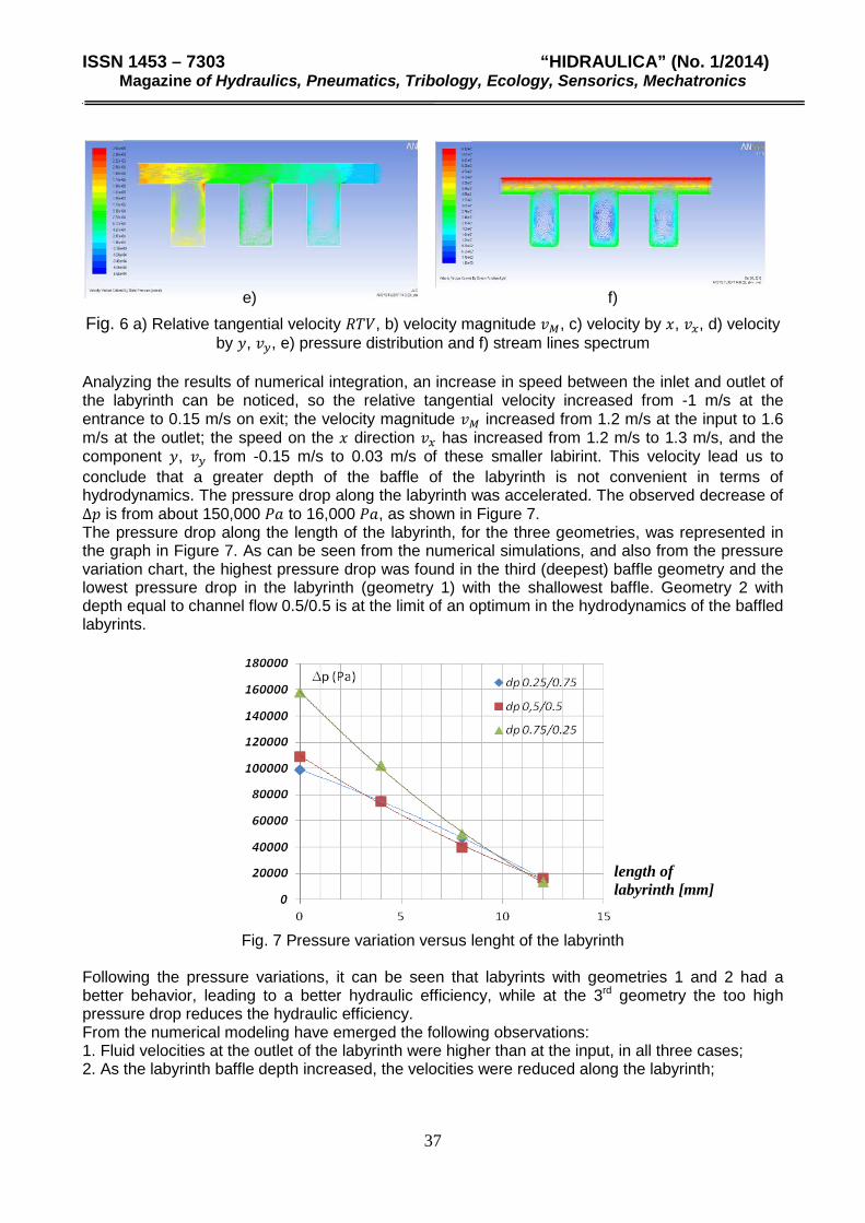
e) f) Fig. 4 a) Relative tangential velocity 𝑅𝑇𝑉, b) velocity magnitude 𝑣𝑀, c) velocity by 𝑥, 𝑣𝑥, d) velocity
by 𝑦, 𝑣𝑦, e) pressure distribution and f) stream lines spectrum From the results obtained it was observed an increase in speed between the inlet and outlet of the labyrinth, so the relative tangential velocity increased from -0.5 m/s at the entrance to 0.6 m/s at the outlet, the velocity magnitude - the resultant velocity representing the 2 directions - increased from 7 m/s at the entrance to 8.7 m/s at the outlet, the speed 𝑣𝑥 on the horizontal direction has increased from 6.8 m/s to 8.7 m/s, and 𝑣𝑦 on the vertical direction from -0.1 m/s at input to 0.6 m/s at the outlet of the labyrinth. Within the baffles, 𝑣𝑀 and 𝑣𝑥 velocities are lower, you can see the vortices formed in the liquid flow and the pressure drop ∆𝑝 along the labyrinth is observed to decrease is from about 100000 𝑃𝑎 to 5500 𝑃𝑎, variation illustrated in Figure 7. The increase in speed is also checked by the pressure drop along the labyrinth. The vortices formed within the baffles ensure proper sealing of the flow, thus leading to the reduction of leakage flow and a better volumetric efficiency.
2.2.2. Modeling of the labyrinth with the geometry 2 The case when the baffle’s depth is equal to the width of the flow channel, 0.5 / 0.5 in parametric design, has led to the the folowing results (Figure 5):
a) b)
b) d)
35
ISSN 1453 – 7303 “HIDRAULICA” (No. 1/2014) Magazine of Hydraulics, Pneumatics, Tribology, Ecology, Sensorics, Mechatronics
e) f) Fig. 5 a) Relative tangential velocity 𝑅𝑇𝑉, b) velocity magnitude 𝑣𝑀, c) velocity by 𝑥, 𝑣𝑥, d) velocity
by 𝑦, 𝑣𝑦, e) pressure distribution and f) stream lines spectrum An analysis of the results obtained showed an increase in speed between the inlet and outlet of the labyrinth, so the relative tangential velocity increased from -3.5 m/s at the entrance to -0.7 m/s at the outlet; the velocity magnitude 𝑣𝑀 increased from 3.88 m/s at the inlet to 4.8 m/s at the outlet; the velocity on horizontal direction 𝑣𝑥 has increased from 3.95 m/s to 4.83 m/s, and the vertical velocity component 𝑣𝑦 from -0.2 m/s at the entrance to 0.2 m/s at the labyrinth’s outlet. Within the baffles, the velocities 𝑣𝑀 and 𝑣𝑥 are much lower, the vortices formed in the liquid flow can be clearly seen, and the pressure drop ∆𝑝 along the labyrinth decreases from about 109000 𝑃𝑎 to 4800 𝑃𝑎 (see also figure 7). From the stream lines spectrum can be observed the formation of vortices in the labyrinth’s baffles, a "dead zone", who ensures the seal between rotor and housing of the turbomachine.
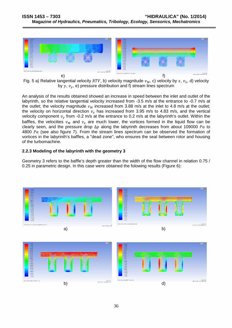
2.2.3 Modeling of the labyrinth with the geometry 3 Geometry 3 refers to the baffle’s depth greater than the width of the flow channel in relation 0.75 / 0.25 in parametric design. In this case were obtained the folowing results (Figure 6):
a) b)
b) d)
36
ISSN 1453 – 7303 “HIDRAULICA” (No. 1/2014) Magazine of Hydraulics, Pneumatics, Tribology, Ecology, Sensorics, Mechatronics
e) f)
Fig. 6 a) Relative tangential velocity 𝑅𝑇𝑉, b) velocity magnitude 𝑣𝑀, c) velocity by 𝑥, 𝑣𝑥, d) velocity by 𝑦, 𝑣𝑦, e) pressure distribution and f) stream lines spectrum
Analyzing the results of numerical integration, an increase in speed between the inlet and outlet of the labyrinth can be noticed, so the relative tangential velocity increased from -1 m/s at the entrance to 0.15 m/s on exit; the velocity magnitude 𝑣𝑀 increased from 1.2 m/s at the input to 1.6 m/s at the outlet; the speed on the 𝑥 direction 𝑣𝑥 has increased from 1.2 m/s to 1.3 m/s, and the component 𝑦, 𝑣𝑦 from -0.15 m/s to 0.03 m/s of these smaller labirint. This velocity lead us to conclude that a greater depth of the baffle of the labyrinth is not convenient in terms of hydrodynamics. The pressure drop along the labyrinth was accelerated. The observed decrease of ∆𝑝 is from about 150,000 𝑃𝑎 to 16,000 𝑃𝑎, as shown in Figure 7. The pressure drop along the length of the labyrinth, for the three geometries, was represented in the graph in Figure 7. As can be seen from the numerical simulations, and also from the pressure variation chart, the highest pressure drop was found in the third (deepest) baffle geometry and the lowest pressure drop in the labyrinth (geometry 1) with the shallowest baffle. Geometry 2 with depth equal to channel flow 0.5/0.5 is at the limit of an optimum in the hydrodynamics of the baffled labyrints.
Fig. 7 Pressure variation versus lenght of the labyrinth
Following the pressure variations, it can be seen that labyrints with geometries 1 and 2 had a better behavior, leading to a better hydraulic efficiency, while at the 3rd geometry the too high pressure drop reduces the hydraulic efficiency. From the numerical modeling have emerged the following observations: 1. Fluid velocities at the outlet of the labyrinth were higher than at the input, in all three cases; 2. As the labyrinth baffle depth increased, the velocities were reduced along the labyrinth;
length of labyrinth [mm]
37

ISSN 1453 – 7303 “HIDRAULICA” (No. 1/2014) Magazine of Hydraulics, Pneumatics, Tribology, Ecology, Sensorics, Mechatronics
3. Equal values of inlet- and outlet-velocities were recorded at geometry 2, for the labyrinth baffle depth equal to channel width 0.5/0.5, which leads to the idea of an optimal configuration for this geometry; 4. The variation of the pressure at the entrance of the maze has led to small velocity variation. Labyrinth’s baffle geometry is essential; 5. Maximum Relative Tangential Velocity levels occur within the baffles, as well as maximum Velocity Magnitudes 𝑣𝑀 and maximum 𝑣𝑦 velocities; 6. The pressure drop along the labyrinth length was different, accelerated the for deeper baffles, when more fluid loses into them; 7. The flow spectrum highlighted turbulent flow by forming vortices in the area of the labyrinth’s baffles, at the flow of the viscous fluid through it, providing the labyrinth seal. These observations led us to the conclusion that an optimal baffled labyrinth has baffles with a maximum depth equal to the width of the fluid flow and the step of the grooves equal to this depth. Numerical simulations and similar conclusions were found in papers [1-4]. 3. Conclusions Numerical modeling of the viscous fluid flow through the labyrints of a turbomachine led to the following observations: fluid flow velocities increase between inlet and outlet of the labyrinth in all three geometries studied; at the deepening of the labyrinth baffle, speeds were reduced along the labyrinth; approximately equal velocity levels were recorded at a baffle depth equal to the channel width (in parametric design 0.5/0.5) - this may represent the optimal configuration for the design of sealing labyrinths with baffles. The pressure drop along the labyrinth was different, more accelerated in the case of deeper baffles. The flow spectrum showed the formation of vortices in the area of the baffles, providing the labyrinth seal. We obtained stable numerical solutions at low speeds through the labyrint (0.5, 5 or 10 m/s). In subsequent experimental research were viewed flows at different Reynolds numbers and the pressure decreases were confirmed. These will be subject to the following article. This research will be extended by further researches on the effect of the geometry in the improvement of the turbomachine’s hydraulic efficiency. REFERENCES [1] Rhode, DL; KO, SH; Morrison, GL (2008) - Experimental and numerical assessment of an advanced labyrinth seal, Tribology transactions 37(4), 743-750. [2] Kirk R.G., Guo Z. (2009) - Influence of Leak Path Friction on Labyrinth Seal Inlet Swirl, Tribology transactions 52(2), 139-145. [3] Liu, Z.P.; Liu, S. L., Zheng, S.Y.(2011), A New Numerical Method to Realize Unsteady Calculation of Flow in Labyrinth Seals, Advances in Mechanical Design, PTS 1 AND 2Book Series: Advanced Materials Research Volume: 199-200, 68-71. [4] Hirono T., Guo Z.L., Kirk R.G. (2005) – Application of computational fluid dynamics analysus for rotating machinery – Part II: Labyrinth seal analysis, Journal of engineering for gas turbines and power transaction of the ASME, Vol 127 (4), 820-826. [5] Cazacu M.D., Budea S. – Curgeri tridimensionale ale fluidelor vascoase prin masini si echipamente, Editura Printech, 2012, 92-112. [6] Cazacu M.D.(2003) – On the boundary conditions in three-dimensional viscos flow, the 5-th Congres of Romanian Matematicians, June 22-28, 24-26.
38
ISSN 1453 – 7303 “HIDRAULICA” (No. 1/2014) Magazine of Hydraulics, Pneumatics, Tribology, Ecology, Sensorics, Mechatronics
MICROSTRUCTURE AND TRIBOLOGICAL CHARACTERISTICS OF
BIOCOMPATIBLE 316 L STAINLESS STEEL
PhD physicist FLORINA VIOLETA ANGHELINA1, PhD Eng. VASILE BRATU 1
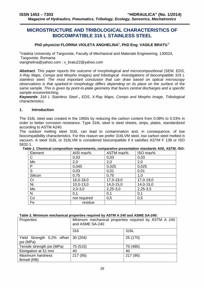
1Valahia University of Targoviste, Faculty of Mechanical and Materials Engineering, 130024, Targoviste, Romania [email protected] ; [email protected] Abstract. This paper reports the outcome of morphological and microcompozitional (SEM, EDS, X-Ray Maps, Compo and Morpho images) and tribological investigations of biocompatible 316 L stainless steel. The most important conclusion that can draw based on optical microscopy observations is that sparked-in morphology differs depending on its place on the surface of the same sample. This is given by point-to-plate geometry that favors central discharges and a specific sample erosion/etching. Keywords: 316 L Stainless Steel , EDS, X-Ray Maps, Compo and Morpho Image, Tribological characteristics. 1. Introduction
The 316L steel was created in the 1950s by reducing the carbon content from 0.08% to 0.03% in order to better corrosion resistance. Type 316L steel is steel sheets, strips, plates, standardized according to ASTM A240. The outdoor melting steel 316L can lead to contamination and, in consequence, of low biocompatibility characteristics. For this reason we prefer 316LVM steel, low carbon steel melted in vacuum. A steel 316L or 316LVM is considered biocompatible if it satisfies ASTM F 138 or ISO 5832-1.
Table 1. Chemical composition requirements, comparative presentation standards AISI, ASTM, ISO: Element AISI max% ASTM max% ISO max% C 0,03 0,03 0,03 Mn 2,0 2,0 2,0 P 0,045 0,025 0,025 S 0,03 0,01 0,01 Silicon 0,75 0,75 1,0 Cr 16,0-18,0 17,0-19,0 17,0-19,0 Ni 10,0-13,0 14,0-15,0 14,0-15,0 Mo 2,0-3,0 2,25-3,0 2,25-3,5 N 0,1 0,1 0,1 Co not required 0,5 0,5 Fe residue
Table 2. Minimum mechanical properties required by ASTM A 240 and ASME SA-240: Properties Minimum mechanical properties required by ASTM A 240
and ASME SA-240
316 316L
Yield Strength 0,2% offset psi (MPa)
30 (204) 25 (170)
Tensile strength psi (MPa) 75 (515) 70 (485) Elongation at 51 mm 40 40 Maximum hardness Brinell (RB)
217 (95) 217 (95)
39

ISSN 1453 – 7303 “HIDRAULICA” (No. 1/2014) Magazine of Hydraulics, Pneumatics, Tribology, Ecology, Sensorics, Mechatronics
Steels type AISI 316 L is a special type of biocompatible material for applications in orthopedics, to obtain which were done extensive research at SC COST SA Targoviste, Valahia University of Targoviste and Polytechnic University of Bucharest. In this case, questions have arisen about compositional analysis with high accuracy to validate their application in clinical practice. [1÷11]. 2. Materials and methods Optical emission spectrometry with spark excitation (OES-Spark Stand) If using high energy discharge in argon atmosphere, a portion of the sample is remelted. The discharge vaporizes only a segment of the sample. The result of the analysis is independent of sample fragment structure remained. The method technique known as HEPS (High Energy Pre Spark) allows calibration with reference materials and / or samples of materials with unknown structures. With this technique you can obtain sufficiently accurate results making some corrections. Detection limits for some elements (eg. Pb, Sb, Bi) require improvements. OES method is complicated and requires a lot of time and abrasive paper. When using standard samples OES analysis for the elements Cr and Ni can record accuracy (2 S)> 1% rel For the spectrochemical test was used Specrolab spectrometer. To clear image of electric spark discharge in argon were investigated both macrostructural and microstructural optical microscopy and electron microscopy, SEM-EDS, sparking areas resulting from OES investigations method and associated studied samples of AISI 316L steel. Determination of microstructure was performed in the laboratory of microstructural analysis of SC COST Targoviste, the laboratory is equipped with line type BUEHLER metallographic sample preparation. Microstructures were visualized with a microscope type REICHERT Univar assisted by a computer equipped with image analysis software. The device is equipped with a high resolution digital camera Type Polaroid DMC 1E type TWAIN driver. Image analysis equipment, has a Frame Grabber type Matrox Meteor II. For SEM investigation of fingerprint evidence spark steel AISI 316L was used electron microscope XL-30-ESEM TMP equipped with ED-RS spectrometer (Fig. 1).
Fig. 1. Overview of electron microscope. XL-30-ESEM TMP.
The microscope is equipped with appropriate software to support the operation, data acquisition and processing of results ie SEM images, ED-XRF spectra etc. (Environmental Scanning Electron Microscope) [12]. Preparation of samples. The samples studied are cylindrical samples (wires) that can be analyzed directly using a special support. Armed with several standard samples first thing we must ensure is that the standards used are similar samples to be analyzed. The more similar in terms of compositional calibration will be even better. When using the technique HEPS sample preparation method has no influence on spectrochemical results as long as the chemical composition of the sample is changed. It takes into account possible decarburization evidence by overheating (cutting or crushing) and chopped material contamination.
40

ISSN 1453 – 7303 “HIDRAULICA” (No. 1/2014) Magazine of Hydraulics, Pneumatics, Tribology, Ecology, Sensorics, Mechatronics
Regarding electric discharge spark OES spectrometry used, it is considered that it would have a temperature of about 30 000 K, which would allow instant vaporization of the material from the discharge. Also, it is known that the electric discharge is primed metallic inclusions in the sample, formed by particles of slag, abrasive particles of the compound or at "paper" eg grinding. corrundum. If the spectrometer was calibrated using standard samples unknown test results (especially for the elements precipitated) are valid when the intensities are measured at steady state. Specific times corresponding pre-spark samples are as follows: For the control samples taken from the melt (steel, bio, and so on) that S <0.05%, pre-spark times are about 5 seconds. To control the melt samples (steel casting), S <0.05% rise times of about 10 s For samples of semi-finished and finished products with S <0.1% during the pre-spark is about 15 seconds.
3. Results and discussions. 3.1. Spectrometric analytical results. Reproducibility of homogeneous samples obtained at different levels of concentrations can be compared with standard data BEC (Background Equivalent Concentration) and depending on the type of item [10,11].
Element type Sample Concentration 5>Bec Concentration BEC soluble Cr, Ni, Mo,Cu 0,3-0,8 1-2 partially precipitated Al, Ti, P 1-2 2-4 precipitate S, As, Pb, Sb 2-4 4-8 It is impossible to make a classification of all elements as separate conditions of the elements depend on the presence or absence of other elements (oxides, carbides, sulfides) and also depend on the speed of cooling and deformation. Calibration curves for C, Cr, Ni are typical of Cr and CrNi steels base. Surface composition is interpreted by registering ratio metal / oxide for Cr and Fe. To measure the passivation, is determined the composition according to the depth, so the majority elements and for those who are in a lower proportion. Below are presented the analysis of alloy 316L, polished mechanically and passivated respectively.
Fig 2.a Fig 2.b
Figure 2a presents the concentration of the elements O, Fe, Cr depending on the depth. In Figure 2.b passivation effect is presented aiming at the report Cr / Fe.
3.2. Their macro and microscopic investigation of areas spark 316L steel samples. Macrostructural investigations. Macroscopic images of the spark areas are shown in Fig.3. a, b. Sample circled in Fig. 3.b was chosen to be investigated by metallographic microscopy and SEM-EDS microscopy. The sample shows four well differentiated sparks that are representative of the spark.
41

ISSN 1453 – 7303 “HIDRAULICA” (No. 1/2014) Magazine of Hydraulics, Pneumatics, Tribology, Ecology, Sensorics, Mechatronics
a) b)
Fig. 3. a) Macroscopic images of samples spark b) detail view.
Investigation metallographic microstructure by optical microscopy. Microscopic investigation spark area. No 1. The image of Fig. 4 presents the overall appearance of the surface spark. For granular appearance of the central area, which is different from the rest of the surface, it is possible to estimate the diameter of the spark. But this is not relevant from the point of view of accuracy, because there is a transition area from the scanned area of the surrounding area which has a diffuse and a non-homogeneous distribution of the incidence of sparks. The picture shows aspects that suggest the existence of pores or pitting in the spark sites. Also in Fig.4 demonstrates unmistakably that the sparked area is not uniformly morphological aspect uniformly .
Fig. 4. Overview of the sparkle area Fig. 5. Overview of the central sparkle area
no. 1 (spark 1-1X) no.1(spark 1-4X). In the Fig.5 morphological aspects of the sparkle area are shown (spark 1). And this picture shows a granular morphology inhomogeneous local but homogeneous at zonal respectively grainy central area is homogenous relief tenths of a millimeter scale.
Fig..6. Detail of the edge of sparkle area No.1 (spark 1-4X)
The image transition area (Fig. 6) has a rougher than that of the morphology of the the central, which may be corroborated with the relevant aspects of Fig. 4
42

ISSN 1453 – 7303 “HIDRAULICA” (No. 1/2014) Magazine of Hydraulics, Pneumatics, Tribology, Ecology, Sensorics, Mechatronics
The most important aspect is metallographic microscopy revealed granular appearance, coarser, the center of the the spark in relation to adjacent areas. On the other hand, observing with the naked eye sparks suggests that marginal sparkle areas are rough. Investigations by scanning electron microscopy. As a result of investigations by optical microscopy, they do not get enough accurate information or covers to elucidate the mechanisms of interaction of spark sample steel AISI 316 L, therefore it was felt that an investigation by scanning electron microscopy as superior optical microscopy investigations. To highlight the microstructure at magnifications of 1500 - 2000X, the most used method is scanning electron microscopy (Scanning Electron Microscope - SEM). The sample was subjected to investigation is sparkle area No.1, Overview of the sparkle zone obtained in the secondary electron (SE Secondary Electrons) is shown in Fig. 7.
a) b)
Fig.7 Overview of the sparkle footprint) image markers b). 4. Conclusions. Conclusions on investigations of samples of AISI 316L by metallographic microscopy. Images spark one central areas suggest a texture attack (Fig. 9 5). Images peripheral areas, of the sparkle area, scattering sparks point out the existence of cracking the "field" full attack, but with less intensity. Explanation could be a net shaped spark, something like a jet shower, which has a significant scattering droplets of water that the incidence of a sand layer generates a small board crevice excavation. Similarly, it can be shown schematically, the morphological profile generated by a spark (Fig. 8).
Fig. 218 Schematic representation the mode to "attack of sparks".
Thus, in Fig.9 is present unprocessed image of the central area of sparkr no. 1. This image was the "signal" input for frame Graber program that attempted to identify distinct structural units based on gray scale uniformity and discrimination of the threshold ("thre shoulding").
43

ISSN 1453 – 7303 “HIDRAULICA” (No. 1/2014) Magazine of Hydraulics, Pneumatics, Tribology, Ecology, Sensorics, Mechatronics
Fig..9 Raw image of the central area, the spark.
1 Tabelul 3. Data related to the image of Fig. 9
Results "structural discrimination / morphological" are given in Table 3. Thus, there are morphological discrimination unit, the minimum area of 13 µm2 with a weight ratio of about 19% of the area under investigation and the maximum structural unit of area of about 300 µm2 in a proportion of about 81%. Thanks the rough form of relief sample and lack of discrimination of thresholds, it is understandable that the data in Table 3 are not exact, but guidance. Detailed analysis of the image of semicentral fingerprint area no. 1 reveals that there is a small gradient transition intensity of the attack, from the center to the periphery. Conclusions on investigations steel AISI 316 L samples by electron microscopy. Of Fig. 7 make clear the overall morphology of the fingerprint spark, that is, it consists of a central location approximately circular (Fig. 417 b), in which the incidence of sparks (individual) to destroy preexisting structure. The area looks like a muddy field into the was raining with stone. This area has a diameter of about 2 mm. Circumscribing the disc is a ring, with the side of about 1 mm (Fig. 41.7 b), in which the incidence of spark bombardment is reduced, however, this crown are the recesses (pitting and crevice s) for which genesis can be assigned to most likely, discharge channels "fixed". Backscatter electron images obtained are intended to highlight the heterogeneous chemical comoziţia the area concerned. COMPO image of Fig.10 followed also highlight possible changes in the distribution of chemical elements into spark area. This picture does not reveal any significant inhomogeneities of chemical composition, but show morphological differences diminish due to the way of obtaining the SEM image.
\ Fig.10 COMPO image of footprint spark.
In conclusion, BSE and COMPO images without relevant information in this case. Elemental analysis to energy dispersive radiation spectrometry (ED-XRS-Energy Dispersion X-ray Spectroscopy-) can be correlated with BS and COMPO investigations to estimate the combined
Analysis Statistics Phase Area Area (µm)
Minimum
Maximum
Mean
Std. Dev.
Field Statistics
Total Scanned Area
Field Area
Number of Fields
18.606% 12.90532
81.394% 2959.621
N/A 167.7805
N/A 261.7775
1784032
1784032
1
44

ISSN 1453 – 7303 “HIDRAULICA” (No. 1/2014) Magazine of Hydraulics, Pneumatics, Tribology, Ecology, Sensorics, Mechatronics
effect of composition, segregation, or distillation of the elements into the sparkle surface. Therefore it was decided that the areas to be analyzed and investigated SEM ED-XRS. Thus, in Fig.11 presented the X-ray emission spectrum characteristic electron beam induced incidents. Of Fig. 11, that in the spark are found all main alloying elements in steel AISI 316 with intensities proportional to the concentrations of those elements.
Element C(%) Cr 17,32 Ni 10,07 Mo 1,39 Mn 1,26 Si 0,62 Cu 1,3 O 2,34 S 0,42 Fe 65,28 Total 100
Fig.11 ED-XRF spectrum obtained throughout fingerprint of the spark Tabel 4. The concentrations associated Fig. 11
Mass concentration C (%) dosed by ED-XRS technique corresponding of spectrum for Fig.11 is given in Table 4. All the evidence we experience light and electron microscopy SEM lead to the idea of a local discharge. Discharges are made through "channels" with relatively large diameters >2 µm, which remains to explain. A discharge channel generates shock waves that expels material as excited atoms, ions, and clusters and particles with diameter < 2 µm. The particles are deposited on the periphery spark and generates a surface appearance to "peach skin". "Peach skin" is the reason why the crown spark appears as black. In fact the crown contains nothing that has black or absorb light, but light is dispersible, or better said is scattered randomly scattered on the incidence at surface with the scattering centers at 0,2÷5 µm that break wavefront. Basically, in the footprint, from the center outward diffusive particle density increases (which break wavefront incident) and practically no longer reflects light. What happens at this level remains to be studied! The fact is that black appearance, the appearance of smoked spot from the center to the interior, is given by metal particles deposited. On the other hand, the center of the sample reflected light as the this smooth area, the sizes of 100-200 µm forming tiny mirrors that reflect the light diffusely. Thus, these investigations found the explanation of black crown spark zone, corresponding samples biocompatible steel AISI 316L.
REFERENCES. [1].Constantin Baciu, ş.a.,”Ştiinţa materialelor metalice”, Ed.Didactică şi pedagogică R.A., Bucureşti,1996. [2].Ghe.Ioniţă ş.a.,”Evoluţia şi proprietăţile materialelor”, Ed. Fundaţia “Metalurgia Română”, Bucureşti,1998. [3]. SR ISO 5832-1:1999, Implanturi chirurgicale. Produse metalice. Partea 1: Oţel inoxidabil deformabil. [4]. Pencea I, Bazele incercarilor spectrochimice de emisie optica prin scanteie si arc electric, Ed. Printech, 2007. [5]. B.Antoszewski, s.a., A study of friction of textured surface, Hidraulica Nr. 1 (23) /martie 2009. [6]. Ilare BORDEAȘU, Ion MITELEA, Mircea Octavian POPOVICIU, Marcela SAVA, Stainless steel cold-work hardening through cavitation , ISSN 1453 – 7303 HIDRAULICA (No. 2/2013),Magazine of Hydraulics, Pneumatics, Tribology, Ecology, Sensorics, Mechatronics. [7]. **A. Nocivin, I. Ciuca, Guide Book of Metallic Biomaterials, litografia UPB, 1998. [8]. L.B.Loeb,Statistical factors in spark discharge mechanisms, Rev.Modern Phys. V. 20. No.1,p.151—160, 1948. [9]. A. Jantschi, Chimie Fizică. Analize Instrumentale, Ed. AcademicDirect, 2004, [10] I. Pencea, M. Branzei, F. Miculescu, M.Pencea, O.Trante, M. Miculescu, The matrix effect on spectrochemical analysis accuracy of AISI 316 biomaterial grades, Journal of optoelectronics and advanced materiales, v.9, No.11, November 2007, p. 3411 – 3414. [11]. Contract CEEX 223/2006, Materiale noi biocompatibile pentru implantologie ortopedica. [12 ] www.thermofisher.com/ .
45

ISSN 1453 – 7303 “HIDRAULICA” (No.1/2014) Magazine of Hydraulics, Pneumatics, Tribology, Ecology, Sensorics, Mechatronics
THE FLOW MODELING ON THE CYLINDER VALVE
Prof. dr. eng. Iulian Florescu1, Assoc. prof. dr. eng. Daniela Florescu2
1,2“Vasile Alecsandri” University of Bacau, [email protected], [email protected]
Abstract: Being performed in a wide range of sizes, cylinder valve has been tested only on hydraulic losses by experimental methods or the values passed and sealing flow. An analysis of flow parameters for different valve openings or hydrodynamic parameters variation in these conditions can give us additional elements of design the optimal mode of operation of the valve. Keywords: cylindrical valve, flow modelling, pressure, velocity, Solidworks Flow Simulation
1. Introduction
Cylinder valve or Johnson cylinder valve after its inventor's name, has a central cylindrical ends placed coaxially surrounded by hydrodynamic flow of water rotationally symmetric, which is fixed to the housing by transverse frames in the form of wings. This area includes the locking of a cylindrical part axially sliding part which provides for a partial closure hydrodynamic flow continues with minimum load losses, Figure 1 [1].
Fig. 1. The components of the cylinder valve [2]: 1 - valve body, 2 - ribs fusel; 3 - intermediate housing 3 '- housing upstream, 4 - ribs fusel
5,6 - closure, 7 - joints, 8 - pivot, 9 - crank, 10 - ring; 11 – collar;
Various types of such valves cylindrical construction were performed according to the destination. In hydropower are used to purge the bottom of the dam or penstocks, are classified according to their size or supply pressure. For sizes up to 1 m (D < 1m) for operation of lock body can be achieved by simple mechanisms, such crank and connecting rod, but the size or high pressure is achieved by actuating the gear wheel and threaded rods, pistons or actuators employed. Water flow direction can be left or right depending on the placement of the valve to the turbine or bottom emptying [1, 2, 4]. Being designed to work at pressures of tens of bars or to cope with unsteady flow situations with high overload, it should be possible flow analysis parameters variations depending on input values and design parameters [1, 5]. This theoretical analysis can be done using dynamic simulations allow the study of the influence of a number of physic-mechanical or constructive parameters. Solid Works Flow Simulation Through
46

ISSN 1453 – 7303 “HIDRAULICA” (No.1/2014) Magazine of Hydraulics, Pneumatics, Tribology, Ecology, Sensorics, Mechatronics
these simulations can take benefit on speed and pressure change some constructive shapes and sizes, which can be reflected in the optimal design of cups types of equipment [6, 7]. Using the calculus presented in [1], [2] and [3] we can analyze the influence of parameters on physical-mechanical construction or operation and hence derive dynamic optimal design of these types of valves. 2. The flow modeling Modeling flow through a cylindrical valve was performed using Solid Works program that allows recording of flow parameter variation at different points of the flow, depending on the modification of the piston stroke. For example have been selected 20 points on each line of the current; first line in the vicinity of the bulb inside the valve, the second line in the middle area of the third flow of water in the vicinity of the outer shell as shown in Figure 2. As the input data are selected the inlet pressure with 4 bars values, and for the outlet pressure is selected the atmospheric pressure.
Fig. 2. Position power lines that are followed hydrodynamic parameters Maximum valve opening is 400 mm and in relation to the position of the shutter will position the openings 100, 200 and 300 mm. For each position of the three current lines are held positioned as in Figure 2. Velocity and pressure distribution for maximum opening of 400 mm is shown in Figure 3, with traceability streamlines with velocity vectors attached and with limits of values of their respective pressure distribution along the flow.
a.
b.
47
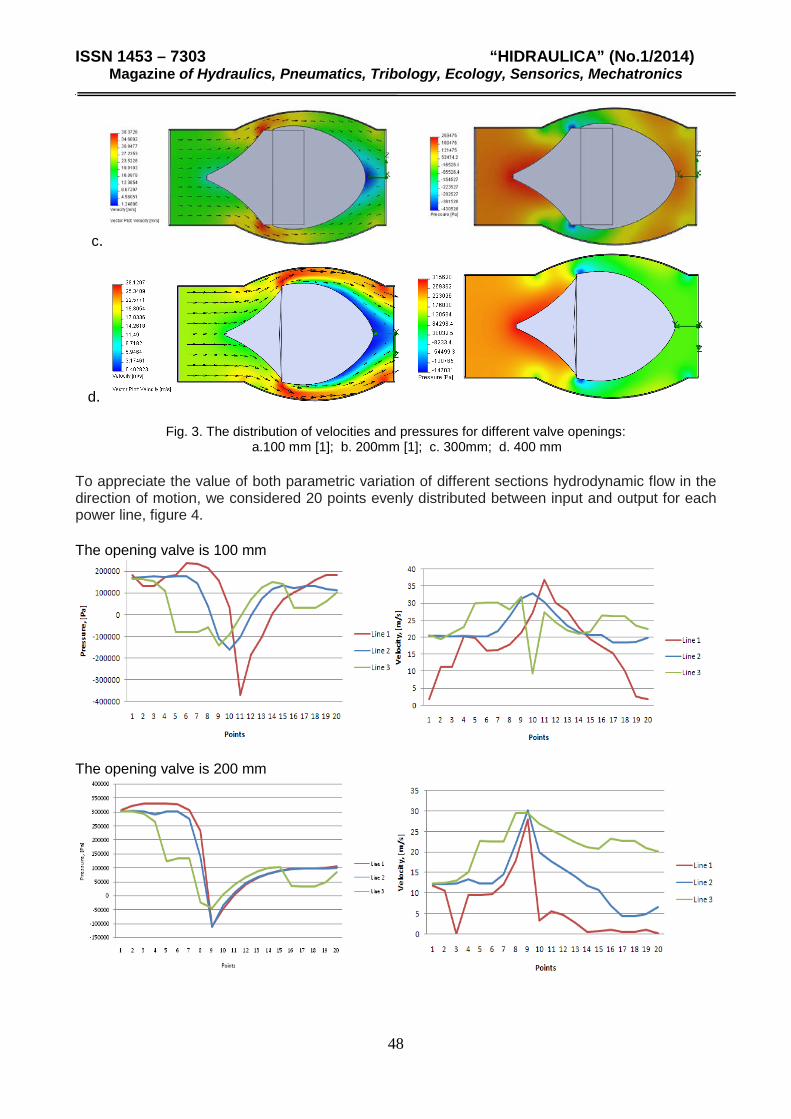
ISSN 1453 – 7303 “HIDRAULICA” (No.1/2014) Magazine of Hydraulics, Pneumatics, Tribology, Ecology, Sensorics, Mechatronics
c.
d.
Fig. 3. The distribution of velocities and pressures for different valve openings: a.100 mm [1]; b. 200mm [1]; c. 300mm; d. 400 mm
To appreciate the value of both parametric variation of different sections hydrodynamic flow in the direction of motion, we considered 20 points evenly distributed between input and output for each power line, figure 4.
The opening valve is 100 mm
The opening valve is 200 mm
48

ISSN 1453 – 7303 “HIDRAULICA” (No.1/2014) Magazine of Hydraulics, Pneumatics, Tribology, Ecology, Sensorics, Mechatronics
The opening valve is 300 mm
The opening valve is 400 mm
Fig. 4. The variations of velocities and pressures for different valve openings:
a.100 mm; b. 200mm; c. 300mm; d. 400 mm Note that the pressure variation along the flow properties keep the allure is the schedule for various openings tends to travel in the direction of flow of minimum with increasing valve opening. For speeds are observed to shift the maximum in the flow direction with increasing valve opening. These two trends are normal relationship between dynamic pressure and water flow rate. Conclusions For different working fluids with mechanical and physical properties and chemical characteristics known we can estimate the flow through the valve section with important dates regarding the main hydrodynamic parameters. You can get such a spectrum of current flow on different lines, variations of pressure and velocity at different points of the valve. It can analyze phenomena such as cavitations in areas where the pressure may drop to low values close to vapor pressure when there is danger of biphasic mixture (vapor of the liquid used). As a consequence of this theoretical analysis of the flow through the valve cylinder can appreciate different design parameters with implications on the reports sections flow through the valve and connecting pipe section. REFERENCES [1] D. Florescu, I. Florescu “Studies on the hydrodynamic flow through the cylinder valve”, Applied Mechanics and
Materials, Trans Tech Publications, Switzerland, Vol. 837 (2014), pp 84-87. [2] Pavel, D., Zarea Şt., „Turbine hidraulice şi echipamente hidroenergetice”, Didactic and Pedagogic Publishing House,
Bucharest, 1968. [3] Florescu, I. „Mecanica fluidelor”, Alma Mater Publishing House, Bacău, 2009. [4] Sajin, T. - Masini mecanoenergetice, Alma Mater Publishing House, Bacău, 2002. [5] Anton, V, Popoviciu, M., Fitero, I. „Hidraulică şi maşini hidraulice”, Didactic and Pedagogic Publishing House,
Bucharest, 1978. [6] I. Florescu, D. Florescu, D. Nedelcu „Studies on the variation of flow parameters through a ball valve”, Applied
Mechanics and Materials, Trans Tech Publications, Switzerland, Vols. 321-324 (2013) pp 1799-1804; [7] I. Florescu, D. Florescu, D. Nedelcu „Hydrodynamic studies on spherical valve”, Applied Mechanics and Materials,
Trans Tech Publications, Switzerland, Vol. 332 (2013) pp 27-32
49

ISSN 1453 – 7303 “HIDRAULICA” (No. 1/2014) Magazine of Hydraulics, Pneumatics, Tribology, Ecology, Sensorics, Mechatronics
INFLUENCE OF CHEMICAL COMPOSITION ON HARDENING PROCESSES, CORRESPONDING FOR ALUMINUM ALLOYS 2024 USED
AT HYDRAULIC EQUIPMENT
PhD Eng. VASILE BRATU 1, PhD physicist FLORINA VIOLETA ANGHELINA1
1Valahia University of Targoviste, Faculty of Mechanical and Materials Engineering, 130024, Targoviste, Romania ; [email protected]
Abstract. In the case of duralumin complex compounds have been identified as: Mg2Si, Al2CuMg, Al7Cu2Fe, etc.This indicates structural complexity for duralumin due to the extensive alloying, complexity that generates multiple factors influence the mechanical, functional, tribological properties. This paper studies the influence of alloying compounds in the emergence hardening phases in aluminum alloys 2024, special destinations use. Keywords: aluminum alloys 2024, chemical composition, hardening processes.
1. Introduction. Compositional analysis of conventional metallic materials (alloys based on Fe, Al, Cu, Co, Ni, etc.) is almost exclusively taken out by spectrometry OES[1,2,3,4,5]. Compositional analysis of special metal materials incumbent special dosing methods and techniques that ensure quality test results as required the estimation their conformity with requirements related (eg Law 608/2001 and SR EN 573-3/2009 [6,7] for aluminum alloys) and Law 608/2001 ISO 5832-1 conjugated and test standards EN 17025 and EN 13005 [see Table A], [8,9]. Spectrometry OES is the most effective technique for compositional analysis of metal alloys. In fact, more or less intentionally, special metal alloys elemental analysis is performed by analyzing OES, either preliminary or routine testing in order to identify the alloy class (eg 2017 or 2024 dural type) or even conformity assessment related specification alloy composition. 2024 type alloys are produced in S.C.ALPROM S.A. Slatina, they can be used on aircraft, electronics and electrical, hydraulic valves bodies, pistons, bushings, orthopedic structures, etc. In order to ensure that the alloy developed can be used in requested it to be characterized in a complex way, that employment must be assessed ie chemical composition chemical compliance with the provisions of SR EN 573 3: 1994 specifies the compositional limits of the alloys in 2024 in percentage by mass:
Table 1. The chemical composition of the alloy 2024 according to EN 573 3:1994.
Element Cu Mg Zn Mn Si Fe Composition SR EN 573 3:1994
3,80.. ..4,90
1,20.. .1,80
max 0,250
0,30 ...0, 90
max 0.50
max 0,50
50

ISSN 1453 – 7303 “HIDRAULICA” (No. 1/2014) Magazine of Hydraulics, Pneumatics, Tribology, Ecology, Sensorics, Mechatronics
Table A.
51

ISSN 1453 – 7303 “HIDRAULICA” (No. 1/2014) Magazine of Hydraulics, Pneumatics, Tribology, Ecology, Sensorics, Mechatronics
Table 2. The chemical composition of the 2024 alloy according to the manufacturer's specifications .
2024 Chemical Analysis Percentage Elements Si Fe Cu Mn Mg Cr Zn Ti Other
elements Total other elements
Al
Val. Min. - - 3.8 0.30 1.2 - - - - - Val. Max. 0.50 0.50 4.9 0.9 1.8 0.10 0.25 0.15 0.05 0.15 rest
On the other hand, the alloy composition is not insured for the proper behavior into service of the alloy because the microstructure (grain size) and content of inclusions and compounds affect the mechanical strength, corrosion resistance and wear resistance, including heat ciclaj generated by temperature variations at required regions. This obviously causes, in addition to determining the chemical composition of the alloy candidate for use in industry to require knowledge pertinent to the nature, size and distribution in the matrix alloy of specific compounds or, worse, that non-specific alloy.
2. Detailing matter
The airline industry and the automobile industry, electrical etc, are used mostly hardenable alloys. Al-Cu binary alloys are used rarely in aviation, but also in industry because of their hardening would be provided only Al2Cu phase (phase θ). Among the many alloys hardened by heat treatment, the most important are those referred duralumin alloy [9,10], which are part of the Al-Cu-Mg alloys with the addition of manganese (and other elements such as Zr, Li, Cr, Be , Ti, Cd, Ag, V). Conventionally, duralumins are divided into three groups, depending on the content of the main alloying elements according to Table 3:
Table 3. Types of duralumin alloy.
Tip duraluminiu % Cu % Mg % Mn % Si % Fe Slab aliat 2,0-3,5 0,2-0,5 0,2-0,5 ≤ 0,7 ≤ 0,6 Mediu aliat 2,5-4,5 0,3-0,8 0,3-0,8 ≤ 0,5 ≤ 0,5 Inalt aliat 3,5-5,0 0,6-1,8 0,6-1,2 ≤ 0,5 ≤ 0,5
Duralumins alloy mechanical strength increases from the low alloy to the high alloy, but at the expense of a decrease in plasticity. Alloy with the highest strength achieved till now is chemically very complex, by 10 alloying elements in Table 4: Table 4. Chemical composition of the aluminum alloy with the high mechanical strength [9].
E Zn Mg Cu Mn Ni Fe Cr Zr B Y Al % 5,5
÷ 7,5
2,3 ÷ 3,6
2÷2,6
0,2 ÷ 0,4
0,3 ÷ 0,5
0,4 ÷ 0,8
0,12 ÷ 0,25
0,25 ÷ 1
0,5 ÷ 0,1
0,15 ÷ 0,25
Rest
Besides alloy composition plays an important role heat treatment conditions applied to it (hardening - aging) as treatment influences the behavior of the alloy in use. Has been found that the rate of hardening has less influence on the mechanical properties and greater influence on the corrosion resistance. Establishing the size of hardening speed is achieved using temperature-time curves - transformation (TTP), similar curves of steels TTT, and built like them.
52
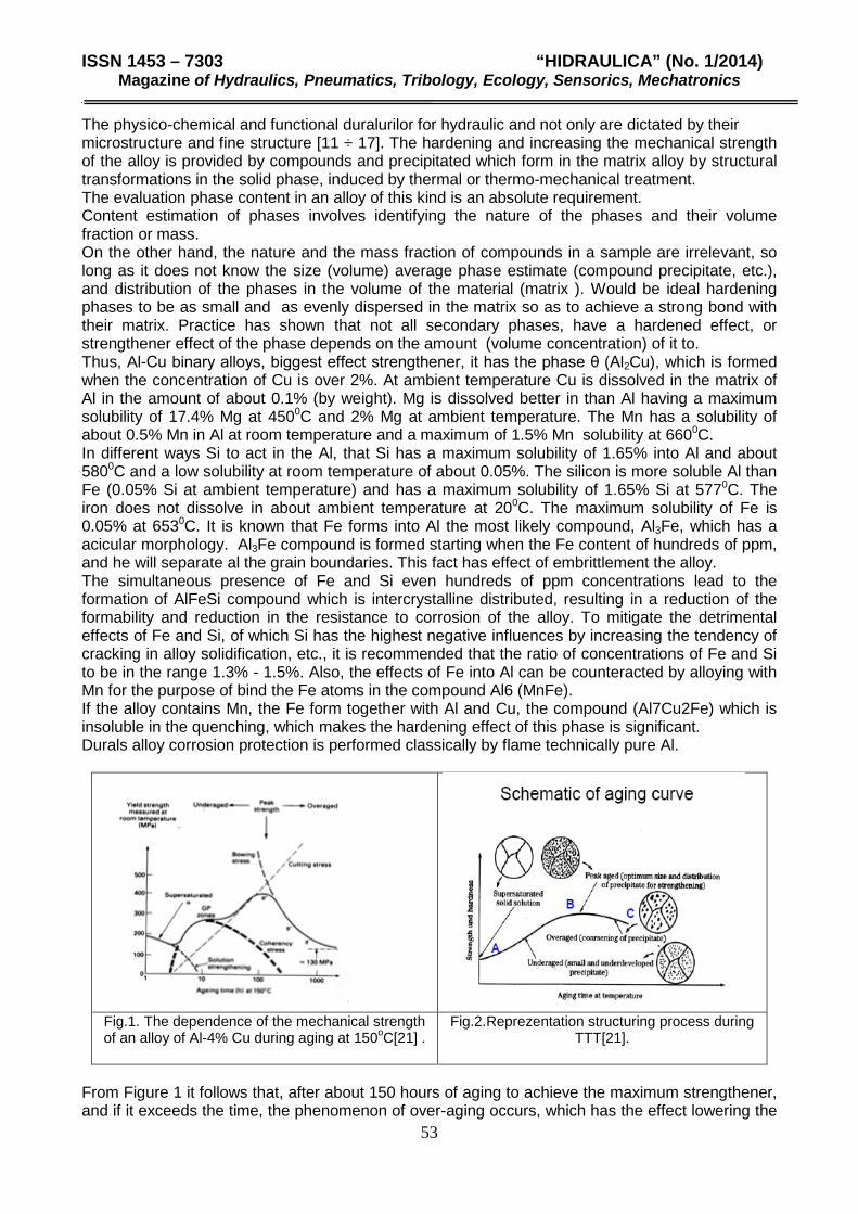
ISSN 1453 – 7303 “HIDRAULICA” (No. 1/2014) Magazine of Hydraulics, Pneumatics, Tribology, Ecology, Sensorics, Mechatronics
The physico-chemical and functional duralurilor for hydraulic and not only are dictated by their microstructure and fine structure [11 ÷ 17]. The hardening and increasing the mechanical strength of the alloy is provided by compounds and precipitated which form in the matrix alloy by structural transformations in the solid phase, induced by thermal or thermo-mechanical treatment. The evaluation phase content in an alloy of this kind is an absolute requirement. Content estimation of phases involves identifying the nature of the phases and their volume fraction or mass. On the other hand, the nature and the mass fraction of compounds in a sample are irrelevant, so long as it does not know the size (volume) average phase estimate (compound precipitate, etc.), and distribution of the phases in the volume of the material (matrix ). Would be ideal hardening phases to be as small and as evenly dispersed in the matrix so as to achieve a strong bond with their matrix. Practice has shown that not all secondary phases, have a hardened effect, or strengthener effect of the phase depends on the amount (volume concentration) of it to. Thus, Al-Cu binary alloys, biggest effect strengthener, it has the phase θ (Al2Cu), which is formed when the concentration of Cu is over 2%. At ambient temperature Cu is dissolved in the matrix of Al in the amount of about 0.1% (by weight). Mg is dissolved better in than Al having a maximum solubility of 17.4% Mg at 4500C and 2% Mg at ambient temperature. The Mn has a solubility of about 0.5% Mn in Al at room temperature and a maximum of 1.5% Mn solubility at 6600C. In different ways Si to act in the Al, that Si has a maximum solubility of 1.65% into Al and about 5800C and a low solubility at room temperature of about 0.05%. The silicon is more soluble Al than Fe (0.05% Si at ambient temperature) and has a maximum solubility of 1.65% Si at 5770C. The iron does not dissolve in about ambient temperature at 200C. The maximum solubility of Fe is 0.05% at 6530C. It is known that Fe forms into Al the most likely compound, Al3Fe, which has a acicular morphology. Al3Fe compound is formed starting when the Fe content of hundreds of ppm, and he will separate al the grain boundaries. This fact has effect of embrittlement the alloy. The simultaneous presence of Fe and Si even hundreds of ppm concentrations lead to the formation of AlFeSi compound which is intercrystalline distributed, resulting in a reduction of the formability and reduction in the resistance to corrosion of the alloy. To mitigate the detrimental effects of Fe and Si, of which Si has the highest negative influences by increasing the tendency of cracking in alloy solidification, etc., it is recommended that the ratio of concentrations of Fe and Si to be in the range 1.3% - 1.5%. Also, the effects of Fe into Al can be counteracted by alloying with Mn for the purpose of bind the Fe atoms in the compound Al6 (MnFe). If the alloy contains Mn, the Fe form together with Al and Cu, the compound (Al7Cu2Fe) which is insoluble in the quenching, which makes the hardening effect of this phase is significant. Durals alloy corrosion protection is performed classically by flame technically pure Al.
Fig.1. The dependence of the mechanical strength of an alloy of Al-4% Cu during aging at 150oC[21] .
Fig.2.Reprezentation structuring process during TTT[21].
From Figure 1 it follows that, after about 150 hours of aging to achieve the maximum strengthener, and if it exceeds the time, the phenomenon of over-aging occurs, which has the effect lowering the
53

ISSN 1453 – 7303 “HIDRAULICA” (No. 1/2014) Magazine of Hydraulics, Pneumatics, Tribology, Ecology, Sensorics, Mechatronics
mechanical strength. The hardening mechanisms of complex alloyed dural involving at least two parallel hardening process by forming sequential phase θ and S phase, respectively [18]: 𝐺𝑃 − 1 → 𝜃 ′′ → 𝜃 ′ → 𝜃(𝐴𝑙2𝐶𝑢) (1) 𝐺𝑃 − 1 → 𝑆 ′′ → 𝑆 ′ → 𝑆 (𝐴𝑙2𝐶𝑢𝑀𝑔) (2) Equilibrium S phase has orthorhombic crystal structure with unit cell parameters: a0 = 0.40 nm, b0 = 0.923 nm and c0 = 0.714 nm [18]. Equilibrium θ phase has tetragonal crystal structure with unit cell parameters a0 = b0 = 0.606 nm, c0 = 0.4874 nm [12,18]. Phase θ ', is a nonequilibrium phase that has a tetragonal structure with unit cell parameters vary depending on the size of the precipitate (phase). Reference values of unit cell parameters are a0 = b0 = 0.404 nm and c0 = 0.508 nm. Also phase θ '' has the tetragonal crystal structure with lattice parameters a0 = b0 = 0.404 nm and c0 = 0.78 ÷ 0.79 nm [18].
3. Materials and methods
For spectrochemical testing of mentioned samples was used optical emission spectrometer by electric spark type Foundry-Master. This is an automated installation, intended elemental analysis of metallic materials, and operates under the control of a soft. Master Foundry spectrometer consists of four main parts :
1. spectrometry apparatus (Fig. 3), 2. process computer 3. preliminary vacuum system (vorvacuum) 4. spectral argon supply installation,
Figure 3. Optical emission by electric spark spectrometer Foundry-Master.
The distributions of elements or conducted with the electron microprobe JXA 50A that operates as a SEM microscope. Main features of the microprobe are maximum accelerating voltage 60kV, 0.86 min scan area 0,86x0,64 µm ; max 6,5x4.5 µm ; magnification 20 -: -1.4 x10⁵x. In this work the results of structural and compositional investigations carried out on samples taken from batches of aluminum alloys "2024" produced by Alro Slatina. Batch studied has AL1 code. The main objective of the investigation is the assessment under these alloys, type specifications (ie in 2024) [19,20], in terms of chemical composition. Subsequently aims microstructural evaluation under the terms of the grain and the effects of hardening natural or artificial aging by the manufacturer.
4. Experimental results.
4.1. Chemical and structural analysis of the charged AL1. Compositional analysis. Semi-finished subjected to the expertise is a 50x50mm rectangular bar. Dosage wet was performed for all elements specified according to EN 515. Since dosing wet prevents estimation uncertainty than by expensive repeating was used optical emission spectrometry determination. Dosage by OSE is extremely important for estimating uncertainties per element and to provide additional control over the exact chemical tests.
54

ISSN 1453 – 7303 “HIDRAULICA” (No. 1/2014) Magazine of Hydraulics, Pneumatics, Tribology, Ecology, Sensorics, Mechatronics
To ensure the quality spectrochemical testing (traceability, uncertainty, etc.) spectrochemical testing OES was performed in accordance with standards EN 17025, EN 13005 and EN 515, ie was performed in a laboratory accredited by RENAR to facilitate the estimate in terms of chemical composition / elements, and it was decided that, along with experimental results to be presented the concentrations required by standard EN 1423 mark . The chemical compositions required, ones wet determined and ones estimated compositions by spectrophotometry are shown in Table 5. Spectrometric compositions are accompanied by uncertainty measurement U (95%), ie 95% confidence level.
Tabelul.5. The reference data and the results dosages.
Concentration Tip Cu Mg Mn Si Fe Cr Ti Zn other elements
cr(%) min 3,80 1,20 0,30 0 0 0 0 0 cr(%) max 4,90 1,80 0,90 0,50 0,50 0,10 0,15 0,25 0,05 cu(%) 4,27 1,62 0,58 0,16 0,24 0,05 0,04 0,25 0,05 cs(%) 4,2 1,52 0,55 0,18 0,21 0,07 0,05 0,21 0,04 Us(95%) 0,1 0,08 0,05 0,04 0,04 0,03 0,02 0,04 0,01
In (Fig. 4) are shown modes of framing the concentrations determined in respect of
concentrations of imposed on.
Fig.4. Comparative representation of specified concentrations of SR 1423 and dosed concentrations.
4.2. Morphological and compositional analysis of the batch AL1 by SEM-EDAX
investigations.
SEM-EDAX investigations have been carried out according to the above specifications, on the sample AL1. The image in (Fig. 5), (650X magnification) shows an area where compounds are highlighted by shades of gray and by form. Thus the white rods are compounds that contain Fe and Cu, at most likely Al7Cu2Fe. Compounds ellipsoidal, or even round, black colored represents strengthener Mg2Si compound. This compound occurs in isolation, and in the vicinity of S phase (Al2CuMg), which has the appearance of baguette. In some areas, these baguettes are agglomerates, forming laced areas of S phase. Position Section: cross.
0.00
2.00
4.00
6.00
Cu Mg Mn Si Fe Cr Ti Zn
Concentrations specified and determined in sample AL1
Cmin SR
C max SR
C umed
C spectrometric
U(95%)
55

ISSN 1453 – 7303 “HIDRAULICA” (No. 1/2014) Magazine of Hydraulics, Pneumatics, Tribology, Ecology, Sensorics, Mechatronics
SEM-EDAX test results: SEM image (Fig. 5) Magnification: 650X. Image size 184x136 µm.
a) magnification 650x b) Right detail central electronic-
increased Fig.5. SEM image of the distribution and morphology of the constituents of the sample AL1. 4. Conclusions 5.
Analyses were performed on batch AL1 highlighted the following conclusions: - The results of Table 5 and Fig.4 : alloy studied falling from the a compositional point of view
in the mark- dural aluminum alloys "2024". - Microstructure, the fineness of grain, was estimated as corresponding to the type of alloy
2024, by an expert metallurgist. - batch shows typical class compounds of dural (Mg2Si, S and S’ phases. Al2CuMg ) and
atypical type compounds Al7Cu2Fe, - In batch studied, is missing the Al2Cu equilibrium compound specified at literature as the
most important strengthener element. This can be explained by the fact that, in the case of batch investigated a dominant precipitation reaction leading to the formation of S-phase (Al2CuMg) and / or the phase S 'according to the scheme:
areas G.P → S '→ S (Al2CuMg)
On the basis of the distributions of elements shown in Fig. 6. have identified the phases:
1) Mg2Si round morphology with apparent diameters in the range 1-10 µm, by "color" black. 2) Phase S (S ') with baguette morphology with lengths of about 15 µm. Also, the phases S
and S ' have a the coalescence phenomena around of some Mg2Si compounds. 3) The compound Al7Cu2Fe is morphologically similar to S phase, and the white color in
lengths of less than about 10 µm.
REFERENCES: [1].K. Slickers, The Automatic Emission Spectroscopy, ISBN 3980.3333-l-0 Brühl Universitäts – Drukerei, Germany, 1993. [2]. I. Pencea, Bazele incercarilor spectrochimice de emisie optica prin scanteie si arc electric, Ed. Printech, 2007. [3]. E. Ţenescu, N. Vlahovici, A. Vancu, Spectroscopie Aplicată, Ed. Did. Ped., 1975. [4]. Truţia, I. Ioniţă, G. Stănescu, Spectroscopie optică, atomică şi moleculară – Lucrări practice, Ed. Univ. Bucureşti, 2003.
56

ISSN 1453 – 7303 “HIDRAULICA” (No. 1/2014) Magazine of Hydraulics, Pneumatics, Tribology, Ecology, Sensorics, Mechatronics
[5]. F.Grigorescu, L. Lupu, Analiza instrumentala in metalurgie si constructii de masini, Ed. Tehnica, Bucuresti, 1986. [6]. *** X-ray Diffractometry(Hardant).doc [7]. Legea nr 608: 2001 - Legea privind evaluarea conformitatii produselor [8]. ****, SR EN ISO/CEI17025:2005 „Cerinţe generale pentru competenţa laboratoarelor de încercări şi etalonări”.www.asro.ro [9]. ****, SR E N 13005., www.asro.ro [10]. N. Popescu, R. Saban, D. Bunea, I. Pencea, Stiinta materialelor pentru Ingineria Mecanica, Editura Fair Partners,Bucuresti 1999. [11]. V. Suciu, M. V. Suciu, Studiul materialelor, Bucuresti, Ed. Fair Partners, ISBN 978-973-1877-01-3, 2007. [12]. C.Baciu, ş.a.,”Ştiinţa materialelor metalice”, Ed.Didactică şi pedagogică R.A., Bucureşti,1996. [13]. Ghe.Ioniţă ş.a.,”Evoluţia şi proprietăţile materialelor”, Ed. Fundaţia “Metalurgia Română”, Bucureşti,1998. [14]. F. Oprea, Z. Bacinski - Introducere în termodinamica materialelor, Ed.Fundaţia Metalurgia Română, 1998. [15].I. Licea, “Fizica metalelor”, Editura ştiinţifică şi enciclopedică, Bucureşti, 1986. [16].Ghe. Zet şi D. Ursu,“Fizica stării solide (aplicaţii în inginerie)”, Editura Tehnică, Bucureşti, 1889. [17]. T.V. Popescu, Executia sistemelor hidraulice prin metalurgia pulberilor, Hidraulica, Nr.1 (21)/martie 2008, ISSN 2343 – 7707 ; ISSN-L 1453-7303. [18].S. Zamarca, F. Vasiliu, I. Pencea, Studiul durificarii duralurilor, Rev. Studii si cercetari de fizica, Vol.109, 1988. [19]. SAE AMS 4037N, Aerospace materials specification; NA 41.100, NA 41.101, NA 41.110, NA 41.118. [20]. EN 515, Aluminium and aluminium alloys, Wrought products-Temper designation; Aluminum standards and data, The aluminum Association May, 2009. [21]***www.http//usersmlr.uiuc.edu/cahil/308/precipitation/pdf. “Precipitation hardening”, January,2009.
57

ISSN 1453 – 7303 “HIDRAULICA” (No. 1/2014) Magazine of Hydraulics, Pneumatics, Tribology, Ecology, Sensorics, Mechatronics
AUTOMATION OF A PUMPING STATION FOR LOW POWER APPLICATIONS
Laurentiu ALBOTEANU1, Gheorghe MANOLEA1, Alexandru NOVAC2 1 University of Craiova, [email protected], [email protected] 2 S.C. Promat S.A., [email protected]
Abstract: The paper shows a solution of automation and monitoring for a pumping station. The monitoring and control is performed locally using a PLC and remotely using a PC. Remote transmission of information from local equipment to computer is performed on a serial RS232 communication network. The experimental results were obtained in real conditions of operation and showed good functioning of the monitoring system
1. Introduction
Starting and stopping the pumps in a pump station can provide manual, semi-automatic and automatic. Due to the high consumption of electricity, the need for continuous surveillance and danger of malfunction, start and stop manual pump is completely abandoned. Automating of starting and stopping pumps can be based on the following parameters:
• Automation a function of time; • Automation a function of fluid level; • Automation a function of pressure; • Automation a function of flow.
This paper presents a solution of automation based on fluid level out of the tanks. Also, the solution provides the user with a choice of pump control: automatic, semi-automatic, or manual.
2. PLC hardware description
2.1. Requirements of PLC design PLC of pumping system must meet the following requirements: - development will be around a microcontroller; - it must be possible to purchase 10 digital signals; - programming will be in a higher level language; - keeping settings will be in an internal EEPROM memory; -user interface will be provided by tandem liquid crystal display and keypad minimum of three buttons; - microcontroller programming will be provided via a connector on the PCB; - it must be possible to link information between it and a PC in RS232 standard; - it must be possible to acquire a unified signal 4-20mA; - order will be provided four relays
2.2 PLC structure Ensuring the requirements mentioned above is possible using a structure developed around a microcontroller product type ATMEGA ATMEL 8535 (Fig. 1). It can identify nine functional entities: microcontroller module, the reference voltage block inputs and digital outputs, TTL-RS232 adapter, keyboard, alphanumeric display, analogue input block and power supply. The output voltage of industrial power supply is 12 V DC. Figure 2 shows the final board components corresponding to PLC. Also it can see electrical circuits located on the back of the PCB board.
58

ISSN 1453 – 7303 “HIDRAULICA” (No. 1/2014) Magazine of Hydraulics, Pneumatics, Tribology, Ecology, Sensorics, Mechatronics
Fig. 1. Block diagram of the PLC for pumping plant
Fig. 2. PLC for pumping system.
The ATMEGA is a low-power CMOS 8-bit microcontroller based on the AVR RISC architecture. By executing powerful instructions in a single clock cycle, the microcontroller achieves throughputs approaching 1 MIPS per MHz, allowing the system designed to optimize power consumption versus processing speed. The AVR core combines a rich instruction set with 32 general purpose working registers. All the 32 registers are directly connected to the Arithmetic Logic Unit (ALU), allowing two independent registers to be accessed in one single instruction executed in one clock cycle. The resulting architecture is more code efficient while achieving throughputs up to ten times faster than conventional CISC microcontrollers. The fluid level sensor is likewise in the form of an electronic module (fig. 3). It consists of two identical cells developed around two NPN transistors. Common electrode has a +5 VDC potential. We analyse the block built around transistor Q1. The diode D2 serves to limit the amplitude of the signal received via the limiting resistor R2. The capacitor C1 acts as a filter to acquired signal. Transistor Q1 is then polarized by means of resistors R3 and R4. Diode D3 protects transistor Q1 against external voltages induced.
Microcontroller Keyboard
TTL-RS232 adapter
Analogic input: 4…20mA
Display
Digital inputs block
Digital outputs block
Power supply
PC
Reference voltage
In Relays
Pressure (4…20mA)
+12V
59

ISSN 1453 – 7303 “HIDRAULICA” (No. 1/2014) Magazine of Hydraulics, Pneumatics, Tribology, Ecology, Sensorics, Mechatronics
GNDGND
D25,6DZ
R62,2K
GND
+5VR1
1K
R2
1K
GNDGND
Q1BC546
Q2BC546
Jos
R32,2K
GND
Jos
D15,6DZ
GND
J1
CON4
1234
GND
GND
R747K
D3
1N4007
R447K
D5
1N4007+
C210uF
Sus
GNDGND
R5
1K
D45,6DZ
J2
CON3
123
+5V
GND
Sus
+C1
10uF
Fig. 3. Fluid level sensor. a) electronic diagram; b) components board.
3. PLC software description
3.1. Requirements of microcontroller software The software must assure: - Scanning of analogue inputs; - Reading ten digital inputs; - The status of system will be signalled by a LCD display; - Acquisition of signals from a keyboard with three buttons; - Interconnection of electronic computer serial port via a UART; - Transmission of data packets to PC organized by a predetermined protocol; - Reception of the PC data packages organized by a predetermined protocol. 3.2 General description of microcontroller software The program (Fig. 5) starts with the initialization of the microcontroller and the variables used. Making various timings is possible by using a sequence of decrement all counters used. Afterwards follows the analogue input acquisition, the ten digital signals and signals associated of keyboard. It then set and printed messages through LCD display.
Fig. 4. Flowchart of microcontroller program The implementation of the algorithm contains all interactions between input quantities and corporate output. The program continues with relay control and processing serial communication.
Start
Display
System initialization
Decrement counters
Digital inputs
Algorithm execution
Relays control
Serial communication
60

ISSN 1453 – 7303 “HIDRAULICA” (No. 1/2014) Magazine of Hydraulics, Pneumatics, Tribology, Ecology, Sensorics, Mechatronics
Except block, execution algorithm consists in all other fundamental elements of program elements that do not change from one application to another. In according to desired application obviously will change the content block ‘’algorithm execution’’. 4. PC software
One of the most important is code sequences which enable data transfer between PC and PLC of pumping installation. The following flowchart (Fig. 5) captures such a procedure.
Fig. 5. Flowchart corresponding to serial communication procedure
Chosen software for application development is Visual Basic. It is commonly encountered in industry, is extremely quick and easy to use interface construction equipment - user. Noteworthy is the fact that it contains an object specializing in serial liaising with other digital equipment, ensuring virtually the only convenient way to transfer data between the PC and the technological processes involved.
5. Electrical plant of pumping system For electrical installation of the pumping system has started from the premise that the pump can operate in two modes: - Manual mode (controlled by operator); - Automatic mode (controlled by PLC). The electric scheme that allows operation in both regimes is shown in figure 6, and electric box of automation is shown in figure 7. Operating mode selection is done by the operator through the three-position switch (Q).
Manual mode operating For the manual operation switches position 1 of the Q switch and the control contactor coil supply k is by with the Bp button. Normally open contact k, connected in parallel with the Bp start push button serves to maintain the start command. Cancellation of command is made with the Bo button. Pump operation indication is made by L lamp, which is supplied as standard pump is running. The last circuit on electrical diagram is the power part of the electrical installation. It contains: F1 fuse for short circuit protection, thermal F2 relay for overload protection, K power contactor for pump drive motor.
yes
Testing packet
presence
Processing data
Download buffer
Data concatenation
Extracting data
Save residuum
61

ISSN 1453 – 7303 “HIDRAULICA” (No. 1/2014) Magazine of Hydraulics, Pneumatics, Tribology, Ecology, Sensorics, Mechatronics
Fig. 6. Electrical diagram of pump station Fig. 7. Electrical box of automation
1-LCD display; 2-keyboard; 3-switch; 4-on-off pushbutton; 5-output relay; 6-lichid level sensors; 7- automaton (PLC); 8- DC power supply; 9- contactor; 10- thermal relay; 11- fuse; 12- output to pump.
Automatic mode operating For automatic operation mode switches Q switch in position 2. In this way the work of operator is taken by PLC.The PLC will be mounted on output a Ka additional relay. Its coil will be supplied at a voltage 12 VDC. Normally open contact relay Ka will be mounted in series with the K contactor coil that powers the pump drive motor. Enabling corresponding of output power coil Ka, will be made based on the protocol required for automatic operation of the pumping system.
6. Experimental results
The experimental results were obtained using the automaton (PLC), a serial cable, a PC and the pumping system. The components of the entire automated pumping system are shown in figure 8.
Fig. 8. Automated pumping system: 1- automation box; 2- laptop (PC); 3- sensors box of storage
tank; 4- storage tank;5 – sensors box of supply tank 6- submersible pump; 7-supply tank.
1
2
3
4
5
6
7
8
9
10
11
12
1
2
4
5
6
3
7
62

ISSN 1453 – 7303 “HIDRAULICA” (No. 1/2014) Magazine of Hydraulics, Pneumatics, Tribology, Ecology, Sensorics, Mechatronics
As has been observed in the implementation of programs for the microcontroller and for PC, the automation system was performed according to the water level in the two tanks. Protocol for automatic operation of the pumping system is as follows: 1. The PLC will control the pump starts when the water level in the storage tank is low (Down level storage tank = 0); 2. The PLC will control the pump stop if the water level in the storage tank is at maximum (Up level storage tank = 0); 3. The PLC will control the pump starts if the water level in the supply tank is at maximum (Up level supply tank = 0), and if the water level in the storage tank is not maximum (Up level storage tank = 1); 4. The PLC will control the pump stop if the water level in the supply tank is at minimum (Down level supply tank = 0). To demonstrate the functionality of automation achieved, the system has been experimented in the next cases: 1. Both tanks filled (fig.9); 2. Storage tank being discharge (fig.10); 3. Storage tank empty (fig.11); 4. Both tanks empty (fig.12). The print screens of the PC graphical interface shown below demonstrate operation of the automatic system in all four practice experimental cases. Graphical interface window of PC contains the following areas of monitoring and control: - the area of analogue input (an analogue channel of pressure); - the area of digital inputs (10 inputs); - the area of outputs relay type (4 outputs); - the area of control program; - the area of display control; - the area of semi-automatic control mode In implementing programs for the microcontroller and PC, has been associated negative logic inputs related to PLC (active input = 0; inactive input = 1) and its outputs, has been associated positive logic (active output = 1; inactive output = 0). The experimental results for the cases considered are shown in figures 9 ... 12.
Fig. 9. Storage tank full, the pump is OFF Fig. 10. Storage tank being empty (Up level sensor inactive)
63

ISSN 1453 – 7303 “HIDRAULICA” (No. 1/2014) Magazine of Hydraulics, Pneumatics, Tribology, Ecology, Sensorics, Mechatronics
Fig.11. Storage tank was emptied. Pump is ON Fig. 12. Both tanks are empty. Pump is OFF
As can be seen from the above figures projected PLC has resources for expansion of application. It has 6 digital inputs and 3 outputs unused. Also it offer the opportunity to achieve the automation by pressure, PLC acquires an analogue signal from a pressure sensor.
7. Conclusions
Infrastructure hardware and software used allows monitoring and control of pumping system in real time. Sensors, electrical equipment and electronic components used in the pumping system have a high degree of accessibility and performance using software and standard interfaces. Using a microcontroller for automation and monitoring of pumping system is a solution that can significantly reduce the number of electronic components and cost of design and development of the made equipment. The results of the experiments carried out of the local and remote automation-monitoring system of the pumping system have emphasized the functionality of all elements and of the overall system. REFERENCES
[1] L. Alboteanu, F. Ocoleanu, Al. Novac, Gh. Manolea, ‘’Remote monitoring system of the temperature of detachable contacts from electric cells’’, Annals of the University of Craiova, Electrical Engineering series, No. 34, 2010; ISSN 1842-4805.
[2] L. Alboteanu, Al. Novac, Gh. Manolea, ‘’Parameters monitoring of Stand Alone Photovoltaic System’’, Annals of the University of Craiova, Electrical Engineering series, No. 33, 2009; ISSN 1842-4805.
[3] C. Nedelcut, Al. Novac, Gh. Manolea, Fl. Ravigan, L. Alboteanu, ‘’The automation and supervision of the cultivation environment for horticulture products – functionary food’’, Buletinul Institutului Politehnic Iasi, Tomul LII Fasc. 5A, Electrotehnica. Energetica. Electronica, 1th International Conference on electrical and power engineering (EPE 2006), 12-14 oct., Iasi, 2006, ISSN 1223-8139, pp. 123-128.
[4] D. Păsculescu, T. Niculescu, "The measurement systems with microcomputers". Annals of the University of Petrosani. Electrical Engineering. Universitas Publishing House. Petroşani-România, 2006. ISSN 1454-8518. Pag. 123-128.
[5] W. Nawrocki, “Measurement Systems and Sensors”, London, ARTECH HOUSE, 2005. [6] Zoller C., Dobra Remus, “Microcontroller Implementation In The Electrical Networks For The Hazardous
Areas”, microCAD 2008, International Scientific Conference, University of Miskolc, Hungary, 2008 [7] *** Microsoft, “MSDN Visual Studio 6.0”. [8]*** www.atmel.com.
64