Isogeometric sizing and shape optimization of thin

HAL Id: hal-01898851https://hal.archives-ouvertes.fr/hal-01898851

Submitted on 18 Oct 2018

HAL is a multi-disciplinary open accessarchive for the deposit and dissemination of sci-entific research documents, whether they are pub-lished or not. The documents may come fromteaching and research institutions in France orabroad, or from public or private research centers.

L’archive ouverte pluridisciplinaire HAL, estdestinée au dépôt et à la diffusion de documentsscientifiques de niveau recherche, publiés ou non,émanant des établissements d’enseignement et derecherche français ou étrangers, des laboratoirespublics ou privés.

Isogeometric sizing and shape optimization of thinstructures with a solid-shell approach

Thibaut Hirschler, Robin Bouclier, Arnaud Duval, Thomas Elguedj, JosephMorlier

To cite this version:Thibaut Hirschler, Robin Bouclier, Arnaud Duval, Thomas Elguedj, Joseph Morlier. Isogeometric siz-ing and shape optimization of thin structures with a solid-shell approach. Structural and Multidisci-plinary Optimization, Springer Verlag (Germany), 2018, 10.1007/s00158-018-2100-6. hal-01898851

https://hal.archives-ouvertes.fr/hal-01898851

https://hal.archives-ouvertes.fr

Noname manuscript No.(will be inserted by the editor)

Isogeometric sizing and shape optimization of thin structures with a

solid-shell approach

T. Hirschler1,3 · R. Bouclier2 · A. Duval1 · T. Elguedj1 · J. Morlier3

Received: date / Accepted: date

Abstract This work explores the use of solid-shell elements

in the the framework of isogeometric shape optimization of

shells. The main difference of these elements with respect

to pure shell ones is their volumetric nature which can pro-

vide recognized benefits to analyze, for example, structures

with non-linear behaviors. From the design point of view,

we show that this geometric representation of the thickness

is also of great interest since it offers new possibilities: con-

tinuous sizing variations can be imposed by modifying the

distance between the control points of the outer surfaces.

In other words, shape and sizing optimization can be per-

formed in an identical manner. Firstly, we carry out a range

of numerical experiments in order to carefully compare the

results with the commonly adopted technique based on the

Kirchhoff-Love formulation. These studies reveal that both

solid-shell and Kirchhoff-Love strategies lead to very simi-

lar optimal shapes. Then we apply a bi-step strategy to inte-

grate shape and sizing optimization. We highlight the poten-

tial of the proposed approach on a stiffened cylinder where

the cross-section along the stiffener is optimized leading to

a final design with smooth thickness variations. Finally, we

combine the benefits of both Kirchhoff-Love and solid-shell

formulations by setting up a multi-model optimization pro-

cess to efficiently design a roof.

Keywords Shape Optimization · Sizing Optimization ·Isogeometric Analysis · Stiffened structures · Solid-shell ·Kirchhoff-Love

B T. Hirschler

[email protected]

1 Univ Lyon, INSA-Lyon, CNRS, LaMCoS UMR 5259

F69621 Villeurbanne Cedex, France

2 Univ Toulouse, INSA-Toulouse, IMT UMR CNRS 5219

F31077 Toulouse Cedex 04, France

3 Univ Toulouse, ISAE Supaero-INSA-Mines Albi-UPS,

CNRS UMR5312, Institut Clement Ader

F31055 Toulouse Cedex 04, France

1 Introduction

Shape optimization is one of the great application of Iso-

geometric Analysis (IGA) since the latter integrates Com-

puter Aided Design (CAD) and analysis (Hughes et al

2005; Cottrell et al 2009). Structural optimization requires

a suitable mix of an accurate geometric description and

an efficient analysis model. The classical Finite Ele-

ment Method (FEM) faces few difficulties originated

from the geometric approximation inherent to the fi-

nite element mesh. Two approaches can be distinguished

in the FEM framework: the CAD-based (Imam 1982;

Braibant and Fleury 1984; Ramm et al 1993; Lund 1994)

and the FE-based (Bletzinger et al 2010; Le et al 2011;

Firl et al 2013; Bletzinger 2014) approach. The CAD-based

approach uses a CAD model to define the shape design

and the corresponding shape parameters. The main prob-

lem is that the finite element mesh has to be generated at

every design update. The FE-based approach consists in

using the spatial location of the nodes as the design vari-

ables. It leads to a high number of design variables and ir-

regular shapes with possible distortion meshes. Expensive

mesh regularization techniques are performed to overcome

the shape design representation (Firl et al 2013; Bletzinger

2014). Beyond this, the IGA concept fills the needs of em-

bedding efficient geometric and analysis models by dis-

cretizing the structure with its intrinsic, computer-aided ge-

ometric definition. This study relies on a Non-Uniform Ra-

tional B-Splines (NURBS) based framework (Cohen et al

2001; Piegl and Tiller 1997; Farin 2002). In fact, before the

development of IGA, NURBS have been used in shape opti-

mization due to their ability to describe smooth design, and

because they offer an attractive way to impose the design

updates (Imam 1982; Braibant and Fleury 1984; Ramm et al

1993; Lund 1994). Finally, since CAD uses the boundary

representation (B-rep), IGA is especially suitable for analyz-

mailto:[email protected]

2 T. Hirschler et al.

ing structures whose geometry is easily derived from a sur-

face, as is the case for shells (Kiendl et al 2009; Benson et al

2010; Echter et al 2013; Dornisch et al 2013; Bouclier et al

2013; Caseiro et al 2014; Cardoso and Cesar De Sa 2014;

Bouclier et al 2015b,a; Caseiro et al 2015). Therefore, iso-

geometric shape optimization of shells is a promising

field whose effectiveness has already been highlighted in

some recent works (Nagy et al 2013; Kiendl et al 2014;

Bandara and Cirak 2017).

Isogeometric shape optimization has been suc-

cessfully applied to a wide range of applications (see

for example (Wall et al 2008; Qian 2010; Nagy et al

2010, 2011; Nguyen et al 2012; Nagy et al 2013;

Kiendl et al 2014; Taheri and Hassani 2014; Fußeder et al

2015; Wang and Turteltaub 2015; Ding et al 2016;

Bandara and Cirak 2017; Herrema et al 2017; Wang et al

2017c,b)). A general procedure, which has been improved

over the years (Daxini and Prajapati 2017), is commonly

adopted. It is based on a multilevel design concept which

consists in choosing different refinement level of the same

NURBS-based geometry to define both optimization and

analysis spaces (Nagy et al 2010, 2011, 2013; Kiendl et al

2014; Wang and Turteltaub 2015). Shape updates are repre-

sented by altering the spatial location of the control points,

and in some case the weights, on the coarse level. The

finer level defines the analysis model and is set to ensure

good quality of the solution. The optimization and analysis

refinement levels are independently chosen which provides

a problem-adapted choice of the spaces. Gradient-based

optimization algorithms are generally called upon to solve

the isogeometric optimization problems cited therein. In

fact, isogeometric shape optimization can provide accurate

sensitivities, especially when geometric properties such as

curvature are involved. Several works tackle the issue of

suitable IGA-based sensitivities which has led to improve

the optimization procedures by reducing the discretization-

dependency during the shapes updates (Wang et al 2017a;

Kiendl et al 2014). From this overview, it can be seen

that main researches focus on modeling and optimization

aspects leading today to an accurate general procedure of

resolution. However, discussion from the analysis point of

view is somehow missing. We believe that this is a crucial

issue especially regarding the shape optimization of shells.

In the framework of isogeometric shape optimiza-

tion of shells, it seems that Kirchhoff-Love NURBS el-

ements have been mainly considered (Nagy et al 2013;

Kiendl et al 2014; Bandara and Cirak 2017), while little re-

search works adopt a Reissner-Mindlin NURBS shell for-

mulation (Kang and Youn 2016). However, the influence of

the shell formulations on the optimization results is not

well-known, and, unfortunately, the choice of one shell for-

mulation rather than another is usually dictated by numer-

ical needs. Thus, the Kirchhoff-Love NURBS element is

attractive due to its low computational cost, but it should

be borne in mind that it is restricted to very thin shells.

In order to provide a broader framework that is also suit-

able for thicker shells, we propose to consider in this

work solid-shell NURBS-based element as well. Indeed,

we believe that the solid-shell element can bring inter-

esting features in the shell shape optimization framework

from both the analysis and the design points of view.

First and foremost, it has been demonstrated that such el-

ements are particularly adapted to compute shells with vari-

able shell thicknesses and with complex behaviors (geo-

metric, material and contact nonlinearities) (Bouclier et al

2013; Caseiro et al 2014; Cardoso and Cesar De Sa 2014;

Bouclier et al 2015b,a; Caseiro et al 2015).

Then, regarding more precisely the design aspect, it ap-

pears that the geometric representation of the thickness of-

fers new possibilities. Indeed, the volume representation of

the structure enables to optimize the thickness profile con-

tinuously by modifying the control point coordinates. In this

respect, Ding et al (2016) highlight the benefits of making

use of a NURBS solid element to accurately represent and

analyze the thickness variations encountered in tailor rolled

blanks. Thickness optimization becomes thus natural with

the solid-shell approach and its inherent continuous tran-

sition between the thin and the thick case appears attrac-

tive in a large range of applications. For example, automo-

tive industry already uses rolling processes to enable weight

reduction and a better use of materials (Kopp et al 2005;

Merklein et al 2014; Hirt and Senge 2014). Blended com-

posite laminate structures also presents continuous thick-

ness transition which has a fundamental role to play in this

context (Adams et al 2004). Regarding the optimization, the

number of design variables is reduced in comparison to

more classic methods using discrete sizing parameters at

the element level. Applying the thickness variations with the

NURBS geometry tends to regularize the problem and it acts

as a filter. Therefore, no additional filtering techniques are

required to avoid undesired phenomenon as, for example,

checkerboard pattern experienced with discrete thickness

approaches (Nha et al 1998; Lam et al 2000). The benefits

of solid-shells must, however, be qualified: the automatic

generation of analysis-suitable volumetric NURBS models

is still a challenging task (Liu et al 2014; Al Akhras et al

2017). All the same, for slender structures the task is afford-

able since the geometry is derived from a surface.

Therefore, this study has two main objectives. Firstly,

we seek to extend the existing methodology to be able to

consider solid-shell elements. Comparisons with Kirchhoff-

Love elements are performed in order to validate the pro-

posed solid-shell strategy. Then, we study the benefits of the

solid-shell formulation for the shape optimization of vari-

able thickness structures, and its interest in carrying out

continuous sizing optimization of shells. Hence, this pa-

Isogeometric sizing and shape optimization of thin structures with a solid-shell approach 3

per is organized as follows. In section 2, we review the

concept of isogeometric shape optimization, and we give

practical aspects on the design parametrization of shells.

In section 3, we remind the basics of the solid-shell and

the Kirchhoff-Love NURBS formulations and specify their

treatment to be used for isogeometric shape optimization.

Section 4 provides optimization examples on which com-

parisons between the optimal results obtained with both

shell formulations are made. In section 5, we apply the

proposed solid-shell strategy for thickness optimization of

shells. We perform an integrated shape and sizing optimiza-

tion on a stiffened cylinder. Then, we combine both bene-

fits of Kirchhoff-Love and solid-shells into a multi-model

approach. The global optimal shape is obtained through a

first optimization by using Kirchhoff-Love shells. Then, the

solid-shell formulation is used to further improve the struc-

tures by optimizing the thickness variation. Finally, section 6

concludes on this work by summarizing our most important

points and motivating future research in this direction.

2 Isogeometric shape optimization of shells

The framework of this study draws on research deal-

ing with isogeometric shape optimization (see for exam-

ple (Kiendl et al 2014; Fußeder et al 2015; Nagy et al 2013;

Bandara and Cirak 2017)). This section reviews the princi-

pal insights of the approach by highlighting main theoreti-

cal points and also practical aspects. In particular, we dis-

cuss the multilevel optimization process and the definition

of design variations in the context of isogeometric shape op-

timization of shells.

2.1 NURBS and Isogeometric Analysis

NURBS are a generalization of B-splines and standard in

CAD and computer graphics for geometry modeling (see

(Cohen et al 2001; Piegl and Tiller 1997; Farin 2002)). Only

the fundamentals are given in the following. For futher de-

tails, the interested read is referred to the references cited

therein. A general expression for a NURBS geometry with

parameter ξ ∈ Rd (d being the dimension of the space) is

written as:

SSS(ξ ) =n

∑I=1

RI(ξ )PI , (1)

where n is the number of control points PI and RI are the

NURBS basis functions. The multivariate NURBS basis

functions RI are obtained as weighted B-splines NI by the

following rational definition:

RI(ξ ) =NI(ξ )wI

W (ξ ), with W (ξ ) =

n

∑k=1

Nk(ξ )wk, (2)

where wI is the weight of the Ith control point. The multi-

variate B-spline functions NI are defined as the tensor prod-

uct of univariate B-spline functions. Finally, the 1D B-spline

basis functions are piecewise polynomials defined by the

polynomial degree p and a set of parametric coordinates ξi

collected into a knot vector Ξ. These B-spline basis func-

tions are obtained recursively using the Cox-de Boor re-

cursion formula (see (Cohen et al 2001)). The concept be-

hind IGA (Hughes et al 2005; Cottrell et al 2009) consists

in discretizing the displacement field using the NURBS

parametrization already introduced to describe the geome-

try:

uuu(ξ ) =n

∑I=1

RI(ξ )UI , (3)

where UI is the displacement corresponding to the Ith con-

trol point. By substituting the NURBS approximations in the

weak formulation of a boundary value problem, a linear sys-

tem to be solved is obtained as in standard FEM.

An interesting feature of NURBS is their high degree of

continuity. If m is the multiplicity of a given knot, the func-

tions are Cp−m continuous at that location. This is attractive

from both design and analysis points of view. In particular,

it allows to define smooth free form shapes with high conti-

nuity. Numerical errors in the analysis are reduced because

the geometry can be exactly preserved. The higher conti-

nuity within a NURBS patch increases the accuracy of the

analysis in comparison to standard FEM where C0 regular-

ity is encountered. Furthermore, NURBS present efficient

refinement procedures which allows to enhance the design

space without changing the geometry nor the parametriza-

tion. In particular, k-refinement, in which order and conti-

nuity of the basis functions are simultaneously increased,

can be performed. In practice and especially in the struc-

tural optimization framework, it is efficient to use the matrix

representation of refinement methods of NURBS. For more

details on refinement strategies of NURBS and their matrix

representation, reference is made to (Piegl and Tiller 1997;

Lee and Park 2002).

2.2 Optimization flowchart

Figure 1 describes the main steps of the optimization pro-

cess. It gets an initial CAD model as a main input. CAD

model has here to be understood as an analysis suitable

NURBS geometry. As an output the optimal shape is given

and, an interesting point to notice is that this shape is a

NURBS geometry too. Therefore, the result is directly us-

able by designers and, thus, for production. There is no need

to re-design the final geometry in a CAD environment as it

would be the case with FE-based optimization.


Shape update

Optimization Model

Run Analysis

Analysis Model

Optimization

algorithm

Optimal Shape

CAD Model

k-refinement

IGA results

No

Yes

design

variables

interesting

features

x

J

k-refinement

Fig. 1 Isogeometric shape optimization flowchart: overview of the main steps of the process.

The optimal NURBS geometry is obtained from an iter-

ative process with three main steps. Each iteration consists

in:

1. updating the current shape in a hopefully better one,

2. running the analysis for this new geometry and then in-

ferring mechanical and/or geometrical properties of in-

terest,

3. computing new design variations to further improve the

structure.

A more detailed description of each step of the process is

given in the following paragraphs.

2.3 Multilevel Design

A major asset of isogeometric shape optimization is the

possibility to properly choose both optimization and analy-

sis spaces (Qian 2010; Nagy et al 2010, 2011; Nguyen et al

2012; Nagy et al 2013; Kiendl et al 2014; Fußeder et al

2015; Wang and Turteltaub 2015; Herrema et al 2017;

Wang et al 2017c,b). A fine NURBS discretization is intro-

duced as the analysis model in order to ensure good quality

computations. Conversely, the optimization model is defined

to impose suitable shape variations. Both spaces describe

the exact same geometry and are initially obtained through

different refinement levels of the CAD model as shown in

figure 2.

It is clear that, the finer the analysis model, the better

the results. The choice of the refinement level used for the

analysis model is principally dictated by the need for re-

alistic computational cost. When it comes to the optimiza-

tion model, the situation is quite different. In this case, the

Initial CAD Model OPTIMIZATION Model ANALYSIS Model

Refinement

Fig. 2 Multi-level design approach: optimization and analysis spaces

describe the exact same geometry and are initially obtained through

different refinement levels of the CAD model (above: NURBS ele-

ments, below: control points).

choice of the refinement level has an impact on the com-

plexity of the optimal shape reached. A coarse optimization

model may provide a simpler optimal shape than a fine op-

timization model. Therefore, few questions can be asked in

order to accurately define the refinement levels for the anal-

ysis and optimization models :

• How different from the initial geometry the optimal

shape is allowed to be ?

• Depending on the intended level of shape variation com-

plexity, how fine should the analysis model be to ensure

reliable results ?

These points are illustrated and discussed in more details in

section 4 of this paper.


Fig. 3 Illustration of the design variations of the hemisphere. Middle control points move in radial directions (top) and boundary control points

are coupled with their neighbors to ensure G1-continuity between patches (bottom).

2.4 Design variables

The isogeometric framework provides a proper and accu-

rate way to vary the geometry. It has long been established

that shape control of NURBS is very comfortable and leads

to smooth optimal design (Imam 1982; Braibant and Fleury

1984; Ramm et al 1993). Indeed, a straightforward and nat-

ural way of modifying the shape of the structure is to move

the control points. NURBS also offer an other interesting

way to apply shape variation by modifying the control point

weights, but this point is not investigated here. As pointed

out by Kiendl et al (2014), for the optimization of free form

shapes it is generally sufficient to use only the control point

coordinates. Nevertheless, note that taking the weights as

design variables may improve the optimal shape by adding

proper shape adjustments if the optimization is performed

on a very coarse NURBS model (Wall et al 2008; Nagy et al

2010; Qian 2010; Nagy et al 2013).

Although attractive, taking the control point coordi-

nates as design variables requires attention. Problems are

similar to those encountered with FE-based optimization

where the FE nodal points are directly used as design

variables. In fact, attention must be paid to mesh dis-

tortion in order to avoid local non-injectivities due to

fold-overs. If the control points are allowed to indepen-

dently move in every spatial direction then the optimiza-

tion process constantly needs to check the mesh quality

and often requires cumbersome mesh regularization tech-

niques (Bletzinger et al 2010; Choi and Cho 2015; Le et al

2011; Nguyen et al 2012; Firl et al 2013). In the context of

isogeometric optimization, links between design variables

and move directions are usually set up to avoid these chal-

lenges (Lee and Hinton 2000; Wall et al 2008; Kiendl et al

2014; Taheri and Hassani 2014; Wang et al 2017c,b). Fig-

ure 3 shows this idea in the case of a hemisphere. By letting

only each design control point moving in the radial direc-

tion, we avoid mesh regularity problems. Moreover, control

points located on patch boundaries are often (but not always)

coupled with their neighbors to ensure a G1 geometric conti-

nuity between patches (Kiendl et al 2009). This prevents the

emergence of kinks during the optimization and it finally

leads to smoother optimal shapes. Linking design variables

may also be relevant to preserve initial shape properties as

reflectional, rotational and translational symmetries. It also

guarantees a reduction in the number of design variables

which leads to lower computational cost and again smoother

optimal shapes.

2.5 Shape gradient and Normalization

A typical shape optimization problem can be formulated as

the minimization of a given objective function carried out

over a set of admissible domains. In this work, we limit

ourselves to the case of minimizing the compliance. Other

objective function could have been considered as the mass,

the displacement of a given material point, the maximal

stress, or the critical buckling load and so on. The design

space is limited by lower bound sl and upper bound su

which surround the ns design variables collected in vector

s = (s1,s2, . . . ,sns). This unconstrained optimization prob-

lem can be defined mathematically as:

mins∈Ω

f (s) where: Ω = s ∈ Rns | sl ≤ s ≤ su

f (s) = 12

F ·U = 12

U ·K ·U.(4)

F denotes the force vector, K the stiffness matrix, and U the

displacement vector which satisfies the equilibrium equa-

tions. Moreover, note that constraints, as for example a max-

imal mass, can be added to this optimization problem. An

illustration regarding a constrained optimization problem is

provided in 5.1.


In order to use a gradient-based optimization algorithm,

the derivatives of the compliance with respect to the design

variables need to be computed. A simple chain rule leads

to the following result (see, e.g., Nagy et al (2010, 2013);

Kiendl et al (2014) for more details):

d f

ds= U · dF

ds− 1

2U · dK

ds·U. (5)

The derivatives of the force vector and stiffness matrix with

respect to the design variables are approximated by first-

order finite differences

dF

ds≈ F(s+∆s)−F(s)

∆s,

dK

ds≈ K(s+∆s)−K(s)

∆s. (6)

Combining equation (6) with equation 5 gives semi-

analytical sensitivities which are easy to compute and of-

fer practical advantages (Lund 1994; Kiendl et al 2014). In

fact, the computation of semi-analytical sensitivities does

not require more development than those necessary to build

the stiffness matrix and the force vector. In addition, what-

ever the shell formulation, computation of the sensitivi-

ties is identical. Note that analytical sensitivities may also

be available, depending on the shell formulation, but re-

quire more numerical development (Cho and Ha 2009; Qian

2010; Nagy et al 2013; Taheri and Hassani 2014; Ha 2015).

In practice, the derivatives of the compliance with re-

spect to the design variables are not directly used as the

search direction. Indeed, it has been shown (Kiendl et al

2014; Wang et al 2017a) that normalization approaches help

to reduce discretization-dependency. As a results, we use

here the diagonally-lumped mapping matrix normalization,

also called sensitivity weighting, which leads to the follow-

ing search directions:

di =− 1

Mii

d f

dsi

, with Mii = ∑k∈Ωi

(∫

DRk dD

). (7)

Geometric factor Mii can be interpreted as the fraction of

surface or volume linked to the ith design variable. It inte-

grates in the physical space D all NURBS basis functions

related to the ith design variable (Ωi lists the indexes of the

control points governed by the ith design variable). Finally,

this normalized semi-analytical gradient can be used in gra-

dient based optimization algorithms as, for example, those

provided in the SciPy package (Jones et al 2001–). In this

work, the SLSQP method is used (Kraft 1988).

3 Isogeometric shell analysis

In this work, two isogeometric shell formulations are en-

visaged to perform the optimization. On the one hand, we

extend the shell shape optimization framework in order to

be able to use solid-shell elements for the modeling. On the

other hand, we consider the already established optimiza-

tion process based on the Kirchhoff-Love elements in order

to compare its results with those provided by the solid-shell

element-based procedure. The two shell formulations, along

with their treatment to be used for isogeometric shape opti-

mization, are introduced in this section.

3.1 NURBS-based solid-shell element

3.1.1 Basics

The solid-shell NURBS element used in this work is the

classical one introduced by Bouclier et al (2013). It is based

on a 3D continuum mechanics-type formulation. The idea

is to take a 3D solid continuum element and, in order to

limit the computational costs, discretize the shell using a

single layer of elements through the thickness. This element

is used in its raw form and no particular treatment (strain-

projection, reduced integration, etc.) is put in place here. To

alleviate locking, the basic strategy of increasing the polyno-

mial degree of the analysis model is performed. Despite the

simplicity of the formulation, this element has shown sim-

ilar behaviours to those of Kirchhoff-Love or of Reissner-

Mindlin NURBS shell elements through several shell bench-

marks (Bouclier et al 2013; Benson et al 2010; Kiendl et al

2009; Belytschko et al 1985). Other efficient NURBS-based

solid-shell elements have been developed to overcome lock-

ing phenomena (Bouclier et al 2013; Caseiro et al 2014) and

to analyze structures with geometric (Bouclier et al 2015b;

Cardoso and Cesar De Sa 2014) and material (Bouclier et al

2015a; Caseiro et al 2015) nonlinearities.

Since based on classical 3D continuum elements, the

standard solid-shell formulation is well-know. We only re-

mind the basics in order to underline differences with the

Kirchhoff-Love NURBS shell formulation. No particular

kinematic assumptions are made on the displacement field uuu.

Therefore, strain and stress fields have six components us-

ing Voigt notation. In the context of small perturbations, the

components of the infinitesimal strain tensor εεε are:

εεε i j =1

2

(∂ ui

∂x j

+∂ u j

∂xi

)∀ i, j = 1, . . . ,32, (8)

where ui denotes the ith component of the displacement at

point M located at (x1,x2,x3) in the Cartesian frame. In IGA,

the displacement field is approximated using the NURBS

functions which enables to build the geometry of the struc-

ture. This implies an approximation εεεh of the strains as fol-


Master surface

Slave surface

P0s

P0m

Pm

P0m

Ps

var1 n1

PsPs

var2 n2

(a) (b)

Fig. 4 Definition of the design variables in the context of solid-shell isogeometric elements. (a) A first set of design variables updates the master

surface and (b) the slave surface follows the shape variation through a second set of variables.

lows:

εεεh = ∑A

BAUA with BA =

RA,1 0 0

0 RA,2 0

0 0 RA,3

0 RA,3 RA,2

RA,3 0 RA,1

RA,2 RA,1 0

, (9)

where UA is the vector of the control variables at control

point A, and RA,i denotes the derivative of the NURBS func-

tion at control point A with respect to coordinate xi. Intro-

ducing the approximation fields into the classical weak for-

mulation leads to the following linear system to be solved:

K ·U = F where Kab =∫

D

[Ba ·C ·Bb

]dV,

Fa =∫

DRa fff dV +

∫

ΓF

Ra FFF dγ ,(10)

and with C the Hooke tensor, fff as body force in D, and FFF as

surface load over the Neumann boundary ΓF .

It has been shown that for solid-shell element it is un-

necessary to increase the degree of approximation of the

functions through the thickness beyond 2. When speaking

of solid-shell elements of degree p, the reader should un-

derstand that degree of p is used in the main directions

(commonly referred to as ξ and η) and that degree 2 is se-

lected trough the thickness of the shell. Finally, this basic

solid-shell NURBS element is nothing other than the classi-

cal IGA solid element. Consequently, being able to perform

shape optimization of shell with this element offers another

attractive interest: with the simplest IGA code in hand, one

can run optimization without any further development.

3.1.2 Imposing shape variations

With solid-shell elements, the structure is described by its

volume and not by its mid-surface. Thus, the standard strat-

egy depicted in section 2.4 needs to be further improved: the

shape control has to deal with volume. A solid-shell is char-

acterized by two outer skins. A natural idea is to define one

of the outer skin as the master surface and the other as the

slave surface. This is carried out in this work in two steps.

A first set of design variables updates the master surface as

it is commonly done with shell structure and as already dis-

cussed. Then, a second set of design variables moves the

slave surface starting from the master surface. This idea is

illustrated in figure 4 which shows the shape parametriza-

tion of a tube.

Each control point from the master surface has its equiv-

alent on the slave surface. If a variable var1 moves the mas-

ter point from initial position P0m to Pm in direction n1 and

a second variable var2 further updates the neighbour slave

point form P0s to Ps in direction n2, then the design update

follows

Pm = P0m +var1 n1, [step1]

Ps = P0s +var1 n1 +var2 n2. [step2]

(11)

By setting additional bounds to var2 we avoid undesir-

able shapes as for example overlapping of the outer skins.

Generally, in shape optimization of shells, the thickness is

kept constant. For this purpose, we apply a simple approach

where the second set of design variables is not included in

the optimization. In other words, same shape variations are

applied on both outer skins. If the optimization model has

a higher degree through the thickness than 1, then the inter-

mediate control points are interpolated between both outer

skin. Finally, the use of solid-shell NURBS element offers

the possibility to optimize through the thickness. The thick-

ness optimization issue seems to be promising (Ding et al

2016), and it is investigated in the present work (see sec-

tion 5).

3.2 Kirchhoff-Love NURBS shell formulation

3.2.1 Basics

At the beginning of NURBS-based shell formulations, struc-

tural model approach was firstly developed (see, e.g., the

initial works of (Kiendl et al 2009) on the Kirchhoff-Love


theory and (Benson et al 2010) on the Reissner-Mindlin

theory, and then, more recently, (Echter et al 2013) and

(Dornisch et al 2013)). The structural model approach is

based on a discretization of the mean surface alone. It leads

to fewer degrees of freedom per element in comparison

with solid-shell element. This is particularly true with the

Kirchhoff-Love formulation where no rotational degrees of

freedom are needed. In return, Kirchhoff-Love shells require

C1 continuity but thanks to NURBS surfaces, this condi-

tion is easily satisfied. IGA based on NURBS surfaces offers

Cp−1 continuity throughout the element. Finally, one should

keep in mind that Kirchhof-Love shells neglect transverse

shear deformations, and thus they are accurate for analyzing

thin structures only.

In the Kirchhoff-Love NURBS shell formulation, the

structure is defined by its mid-surface D and its thick-

ness t. In the IGA concept, the mid-surface is described by

a NURBS function S providing at each material point x ∈ D

a straightforward parametrization in terms of a system of

curvilinear coordinates as

x(ξ ,η ,ζ ) = S(ξ ,η)+ζ a3(ξ ,η), − t

2≤ ζ ≤ t

2. (12)

The unit normal a3 and the standard covariant vectors of the

mid-surface aα are given by

a1 =∂ S

∂ξ= S,ξ , a2 =

∂ S

∂η= S,η , a3 =

a1 ×a2

|a1 ×a2|. (13)

The displacement at each material point on the whole struc-

ture is directly linked to the displacement on the mid-surface

uuu. This is the result of the well-know Kirchhoff kinematic

assumptions: straight lines normal to the mid-surface are

characterized by rigid-body displacements and remain nor-

mal to the mid-surface after deformation. It follows that the

linearized strain tensor of the shell is found to be of the form

εεεαβ = eeeαβ +ζ κκκαβ , (14)

where membrane strains eee and bending strains κκκ are given

by

eeeαβ =1

2

(uuu,α ·aβ + uuu,β ·aα

), (15)

κκκαβ =−uuu,αβ ·a3 (16)

+1

|a1 ×a2|[uuu,ξ ·

(aα ,β ×a2

)+ uuu,η ·

(a1 ×aα ,β

)]

+a3 ·aα ,β

|a1 ×a2|[uuu,ξ ·

(a2 ×a3

)+ uuu,η ·

(a3 ×a1

)].

Greek indices take the values 1 and 2. In fact, the kinematic

assumptions vanish the transverse shear strains εεεα3 = 0. As

for the mid-surface, the displacement field is approximated

using the NURBS basis functions. Introducing the approxi-

mation uh into (15) and (16) gives the membrane and bend-

ing strains as follows:

eee(uh) =n

∑i=1

Bmi Ui , and κκκ(uh) =

n

∑i=1

Bfi Ui, (17)

where the matrices Bmi and B

fi can be found in A.1. The

equilibrium configurations of the shell follow from the prin-

ciple of minimum potential energy which, once expressed in

weak form, leads to the linear system

K · U = F where:

Kab =∫

Dt Bm

a ·H ·Bmb + t3

12B

fa ·H ·B f

b dA,

Fa =∫

DRa ppp dA+

∫

Γt

Ra ttt dγ ,

(18)

and with ppp as distributed loads per unit area of D, ttt as axial

forces per unit length of border Γt , and H the material ten-

sor describing the linear elastic behaviour of the shell. Its

expression is given in A.2.

3.2.2 Multi-patch analysis

By comparing the basic solid-shell NURBS element with

the Kirchhoff-Love NURBS shell element, it is clear that

the first is simpler. In addition to this practical aspect,

Kirchhoff-Love element faces some difficulties when it

comes to enforce the G1-continuity between patches, fix

the angle between surface folds, enforce symmetry con-

ditions and prescribe rotational Dirichlet boundary condi-

tions. Computational formulations to overcome these dif-

ficulties are usually either expensive or difficult to imple-

ment and this issue is still of interest (Apostolatos et al

2015; Guo et al 2017; Duong et al 2017; Coox et al 2017).

In this paper the bending-strip approach (Kiendl et al 2010;

Goyal and Simeon 2017) is used to handle multi-patch dis-

cretization and thus, in particular, to perform the coupling

between stiffeners and panels when a stiffened structure

is investigated. The idea is to introduce additional patches

of fictitious material, namely the bending strips, where the

patches are joined with C0 continuity. The material has zero

membrane stiffness and non-zero bending stiffness only in

the direction transverse to the strip. In practice, adding the

bending strips consists in adding terms to the global stiff-

ness matrix introduced in 18. The stiffness matrix of a bend-

ing strip is the same as the one of a classical Kirchhoff-Love

NURBS patch, except the material tensors:

Kbnd-strip

ab =∫

D

t Bma ·H ·Bm

b + t3

12B

fa ·Hbnd-strip ·B f

b dA.


Cylinder (a) Hemisphere(b)

Height H 600 -

Radius R 300 10

Thickness t 3.0 0.04

Modulus E 3.0×106 6.825×107

Ratio ν 0.30 0.30

Loading Local loads Local loads

F = 1 F = 2

Fig. 5 Numerical examples to investigate the use of isogeometric solid-shell elements for shape optimization of shell structures: (a) pinched

cylinder and (b) pinched hemisphere.

The membrane material tensor is null and the bending ma-

terial tensor Hbnd-strip

is given by

Hbnd-strip =P

T ·Hbnd-strip ·P, Hbnd-strip =

E 0 0

0 0 0

0 0 0

(19)

and with E as the directional bending stiffness. Matrix

Hbnd-strip

describes the stress-strain relationship in the local

coordinate system defined by:

e1 =a1

|a1|, e2 =

a2 − (a2 · e1)e1

|a2 − (a2 · e1)e1|, e3 = a3. (20)

Finally, matrix P maps the components of the strain tensor

with respect to the contravariant basis vectors to those with

respect to local orthonormal basis ei.

4 Investigation on preliminary optimization examples

4.1 Description of the numerical examples

In order to investigate the use of isogeometric solid-shell el-

ements for shape optimization of shell structures, two opti-

mization examples depicted in figure 5 are first studied. The

motivation is to ensure compatibility of solid-shell NURBS

elements with isogeometric shape optimization. The effec-

tiveness of the isogeometric Kirchhoff-Love shell formula-

tion for shape optimization of thin structures no longer needs

to be proven. Therefore, there is a great interest in compar-

ing the optimum results obtained by solid-shell elements to

those obtained by the Kirchhoff-Love formulation.

Both the pinched cylinder and the pinched hemisphere

are known from the shell obstacle course (Belytschko et al

1985). These optimization problems are non-convex and are

numerically challenging. In fact, the pinched hemisphere

and the pinched cylinder are commonly studied to test high-

efficient shell elements. The hemisphere is challenging in

terms of locking: it exhibits almost no membrane strains.

The pinched cylinder is even more severe. The loading and

the displacement boundary conditions lead to a highly lo-

calized strain state. The local loading associated with the

curved geometry make the problem challenging numeri-

cally in terms of both locking and representation of com-

plex membrane states. Optimizing this set of problems au-

tomatically requires accurate analysis results. Approxima-

tion error of sensitivity analysis can lead to different local

minimum and unfortunately lead to poor optimal geome-

try (Kiendl et al 2014).

4.2 Pinched cylinder

We first deal with the test case of the pinched cylinder (see

figure 5(a)). The optimization model is chosen relatively

coarse in order to keep the shape simple. Because of the

complexity of the strain state generated by the local loading,

a fine optimization model would lead to a too complex fi-

nal shape. Due to the symmetry of the problem, one eighth

of the cylinder is considered, hence only one NURBS patch

is needed. In the framework of the results presented in fig-

ure 6, the optimization model is built with uniform knot

vectors which discretize the patch in 3 and 4 elements in

the circumferential and the axial direction respectively. De-

gree 2 is chosen in both directions. With such an optimiza-

tion model in hand, 6 design variables update the geometry

as depicted in figure 6(a). Variables named xi move some

control points in the x-direction, whereas variables denoted

ri move some control points in the radial direction. At the

patch boundaries, groups of two or four control points are

set in order to preserve a smooth G1-continuous shape as ex-

plained in figure 3. All variables are constrained by bounds

of [0,60]. Analysis is performed with cubic elements. Re-

finement level of 4 and 3 are set in the circumferential and


Fig. 6 Shape optimization of the pinched cylinder: (a) 6 design variables update the optimization model, (b) final shapes obtained by both shell

formulations, and (c) comparison of the final shapes depicted as the distance between their mid-surface.

Fig. 7 Shape optimization of the pinched hemisphere: (a) 25 design variables update the optimization model, (b) final shapes obtained by both

shell formulations, and (c) comparison of the final shapes depicted as the distance between their mid-surface.

the axial direction respectively, leading to an analysis model

of 1536 elements.

We run the shape optimization with Kirchhoff-Love

NURBS shell elements and with Solid-shell NURBS ele-

ments. Final shapes are identical as shown in figure 6. The

difference between both results is not visible when look-

ing at the design modifications. To further compare the re-

sults, the distance between the mid-surfaces is presented.

The maximum gap between the optimal surface obtained by

Kirchhoff-Love elements and the final mid-surface obtained

by Solid-shell elements is about 0.5 which is, by compari-

son with the range of allowed design variation, very small.

The maximum gap normalized by 60 is lower than 1%. Ta-

Table 1 Optimal values of the design variables for the shape optimiza-

tion of the pinched cylinder.

x1 x2 x3 r1 r2 r3

Kirchhoff-Love 60.0 22.65 7.52 0.0 1.74 0.23

Solid-shell 60.0 23.31 7.58 0.0 1.72 0.51

Relative Gap [%] 0.0 1.10 0.10 0.0 0.02 0.47

ble 1 gives the optimal values of the design variables for

both shell formulations. Results are similar and the relative

gap (defined as |sKL − sSolid|/60) for each variable does not

exceed 1%.

The small difference in final design when using either

Kirchhoff-Love elements or Solid-shell elements may be

a result of the difference in converged solutions. It has be

shown that the converged solution using NURBS solid-

shell elements for the pinched cylinder problem is a lit-

tle softer than the reference solution (Bouclier et al 2013;

Hughes et al 2005). This little difference in solution may

influence the shape updates and finally lead to a slightly

different optimal design. Beyond that, the shape optimiza-

tion of the pinched cylinder reveals very similar behavior

for both shell formulations. During the optimization process,

the shape updates are similar and it has been observed that

the convergence is reached after the same amount of itera-

tions.


Fig. 8 History of compliance and shape during the optimization of the pinched hemisphere when using Kirchhoff-Love NURBS shell elements

and NURBS-based Solid-shell elements.

4.3 Pinched hemisphere

The second example of the pinched hemisphere helps us to

further investigate the use of solid-shell NURBS elements

for shape optimization of shells. Note that the same test case

has been conducted by Kiendl et al (2014) in the context

of isogeometric shape optimization. The symmetry of the

problem allows to consider only one quarter of the structure.

Hence, only one NURBS patch is needed. The optimization

model is built with uniform knot vectors which discretize

the geometry in 5 quadratic elements per parametric direc-

tion. 25 design variables depicted in figure 7(a) are defined

in order to prescribe the shape modifications in radial di-

rection. Once again, the boundary control points are cou-

pled in order the preserve a smooth G1-continuous shape.

All variables are constrained by bounds of [−1, 1]. Further

k-refinement is applied to perform the analysis, leading to an

analysis model with 400 cubic elements. Tests showed that

this refinement level was adequate to converge to the good

looking optimal design.

Once again, we run the optimization with the Solid-

shell NURBS elements and compare the results with those

provided by Kirchhoff-Love NURBS elements. Figure 7(b)

presents the optimal design obtained by both formulations.

Despite the complexity of this optimization problem, the

final shapes are very similar: no visible difference can be

observed. Similar hollows and bumps are located on both

optimal designs. To compare more in detail the results, the

distance between the two mid-surfaces is computed (see fig-

ure 7(c)). The maximum gap in shape is about 6.34 · 10−3

which is very small in comparison with the allowed range

of design modification. Normalized by 2, the maximum rel-

ative distance between the optimal mid-surfaces is lower

than 0.5%. Final values of the cost function also demon-

strate the similarity between the optimal design obtained

with the solid-shell NURBS elements and the one obtained

with the Kirchhoff-Love NURBS elements. The final com-

pliance is 1.34 ·10−3 for the solid-shell case and 1.30 ·10−3

for the Kirchhoff-Love case. However, the final shape ob-

tained by Kirchhoff-Love NURBS elements is not better.

Note that in order to correctly compare the final shapes,

the compliance has to be evaluated on the same analysis

model (Kiendl et al 2014). Strain energy is evaluated for the

optimized shapes in a post-processing step using a fine mesh

with quartic Kirchhoff-Love NURBS elements. This post-

processing procedure reveals that both shapes give a final

compliance of 1.34 ·10−3 which is 1.5% of the initial value

9.24 ·10−2.

Beyond the similarity in final shape, the whole optimiza-

tion histories look alike. Figure 8 shows the convergence

of the objective function in both cases either with solid-

shell NURBS elements or with Kirchhoff-Love NURBS el-

ements. Optimization processes converge at the same speed

and stop after an equivalent number of iterations within a

given tolerance on function value. Some of the intermediary

shapes are also shown in figure 8. Shape updates are very

similar and the different hollows and bumps appear at the

same iteration during the optimization.


5 Application to shape optimization of structures with

variable thickness

The volume representation of the structure offers the possi-

bility to optimize the thickness profile continuously. This in-

teresting feature is investigated through two examples. First,

simultaneous shape and thickness optimization is performed

on a stiffened cylinder. Secondly, we present a multi-model

approach to combine benefits of both Kirchhoff-Love and

solid-shell formulations.

5.1 Stiffened cylinder: shape and sizing optimization

Fig. 9 The stiffened cylinder: two stiffeners are added to the initial

pinched cylinder test case. The left side depicts a global 3D view of

the problem. The right side shows a top view of one quarter of the

stiffener and its cross-section for several angles (Notes: thickness is

magnified by a factor of 4 for better visualization; this detailed view of

the stiffener will be useful to depict the optimal designs in figure 11).

The test case of the stiffened cylinder on which both

sizing and shape optimization will be performed is derived

from the already discussed pinched cylinder problem (see

figures 5 and 6). Two stiffeners are added to the cylinder

as depicted on figure 9. The stiffeners are located at heights

150 and 450. Initially, these stiffeners have a constant rect-

angular cross-section of height 30 and thickness 3. The other

geometric and material parameters are detailed in figure 5.

The optimization problem consists in modifying the cross

section along the stiffeners in order to improve the global

stiffness of the structure. A volume constrain is set in order

to keep the final volume lower or equal to the initial one V0.

Due to the symmetry of the problem, only an eighth of the

structure is considered.

The optimization procedure is done here in two steps.

Height and thickness of the stiffener are optimized one-

by-one. Since the thickness is much less sensitive than the

height, combining both quantities in a single optimization

problem may lead to mostly modify the height of the stiff-

ener. From here on, the shape step denotes the change in

height and the sizing step denotes the change in thickness. A

(a) Height modification:

(b) Thickness modification:

Fig. 10 Shape and sizing optimization with solid-shell NURBS based

elements: the cross-section of the stiffener can be geometrically

parametrized and thus optimized. Here, for each section of control

points, two variables var1 (a) and var2 (b) impose local design modi-

fications in the height and in the thickness directions respectively

first set of design variables hhh updates the height of the stiff-

ener as depicted on figure 10(a). A second set of design vari-

ables ttt modifies the thickness as shown in figure 10(b). Ob-

viously, the design parametrization is not unique. Depending

on how complex the final shape is allowed to be, a simpler

or finer parametrization can be chosen. However, this ex-

ample shows that using solid-shell NURBS based elements

offer an interesting way to optimize through the thickness.

Smooth and continuous thickness variations can be imposed.


(a) Shape only

(b) Shape and sizing optimization

Fig. 11 Optimization results of the stiffened cylinder: (a) final shape when only the stiffener height is modified, and (b) final shape when both

height and thickness are optimized. From left to right are depicted a general 3D view of the final shapes, a top view and several cross sections of

the final stiffeners, and the displacement fields for these two optimized designs (annotations on figure 9 can be helpful to understand the detailed

views of the stiffener).

In this work, the optimization problems behind the shape

step and the sizing step are different. The shape step con-

sists in minimizing the compliance C with a maximal vol-

ume constrain. An additional bound is set in order to limit

the height of the stiffener h in the range [25, 100]. The siz-

ing step minimizes the volume V under the constrain that

the final compliance is lower or equal to the one obtained

from the shape step C*. The design space for the thickness

t is limited to [0.5, 3.0]. The global optimization process is

made of sequences of a shape step followed by a sizing step.

The fixed point process iterates until the global convergence

is reached; that is, convergence on the design variables, the

compliance and the volume. The kth sequence takes the fol-

lowing form:

Minimize C

such that 25 ≤ h ≤ 100

V ≤V0

hhhk, tttk hhhk+1, tttk

C*

1. Shape Step

(21)

Minimize V

such that 0.5 ≤ t ≤ 3.0C ≤C*

hhhk+1, tttk+1hhhk+1, tttk

C*

2. Sizing Step

(22)

Both optimization problems are complementary. The shape

step will use all the available material in order to minimize

the compliance. The sizing step rearranges the material dis-

tribution through the thickness in order to save material.

Then, this saving material can be further use in the shape

step in order to continue minimizing the compliance. This

sequential optimization strategy is sensitive to the initial

starting point and may lead to local optimum. The height and

the thickness design variables are decoupled. Thus, to ensure

a good quality result, we performed a multi-start algorithm.

On top of that, we notice that multidisciplinary optimization

strategies could be of interest to properly solve this problem

and we refer the interested reader to Balesdent et al (2012)


Fig. 12 Optimization history of the bi-step approach applied to the

stiffened cylinder problem. Three global iterations with successive

shape and sizing steps are preformed until convergence. Red zones de-

note the shape steps where the compliance is minimized and blue zones

denote the sizing step where the volume is minimized.

and Martins and Lambe (2013) for futher details regarding

this point.

The results of this study are given in figure 11. More pre-

cisely, figure 11(a) presents the optimal design when only

the height of the stiffener is modified and figure 11(b) de-

picts the final design when both shape and sizing optimiza-

tions are performed. Optimizing through the thickness leads

to a better design in the sense of the compliance. It helps to

make a better use of the material volume. By reducing the

thickness in some locations, the height of the stiffener can

be increased in others. The initial compliance C0 in the case

of a straight stiffener is about 1.73e-06. When only shape

optimization is employed, the final compliance C1 is about

1.68e-06. The final compliance C2 when both shape and

sizing optimizations are performed is about 1.64e-06. The

compliance gain can be defined as Gi = 1−Ci/C0. There-

fore, the compliance gain G2 when adding the sizing op-

timization is almost twice the compliance gain G1 when

only the height of the stiffener is taken into the optimiza-

tion process. Figure 12 depicts the optimization history. It

takes three global iterations to converge. The main design

changes are imposed during the first stage (i.e. the first suc-

cession of a shape and a sizing step) and the second shape

step. For this optimization case, these steps may be enough

to get an optimal geometry. Finally, this example shows that

the solid-shell NURBS element offers an interesting way to

deal with sizing optimization. It extends all the advantages

of the NURBS parametrization to sizing optimization prob-

lem.

5.2 Multi-model optimization

In this last example, we present a multi-model optimization.

The idea is to combine the potential of both Kirchhoff-Love

and Solid-Shell formulations. In a first stage, the Kirchhoff-

Love formulation is used to perform a shape optimization in

which the shell structure is varied in the out-of-plane direc-

tion. Then, the optimal surface is used to generate a volume

model of the structure. In the second stage, thickness opti-

mization is done on the volume model by using the devel-

oped solid-shell approach. We notice that this multi-model

optimization appears consistent since it corresponds to the

design process of structures. The first stage is the proto-

typing in which the influence of many parameters is stud-

ied. It requires a model with low computational cost in or-

Fig. 13 Optimal shape of a square plate subjected to an uniform snow

load: (a) 3D view, (b) top view and (c) side view of the final structure.

Red points represent the control points.


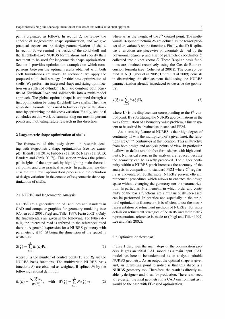
Fig. 14 Variable thickness roof: evolution of the compliance, the volume and the thickness distribution during the optimization.

der to perform many simulations. Once the global shape of

the structure is obtained, an high-fidelity volume model is

created. Instead of directly using this model to generate the

CAD drawings, one can perform a last optimization to apply

final adjustments. Thank to the isogeometric approach, the

final geometry can directly be transferred to the manufactur-

ing step since no conversion in a CAD format is required.

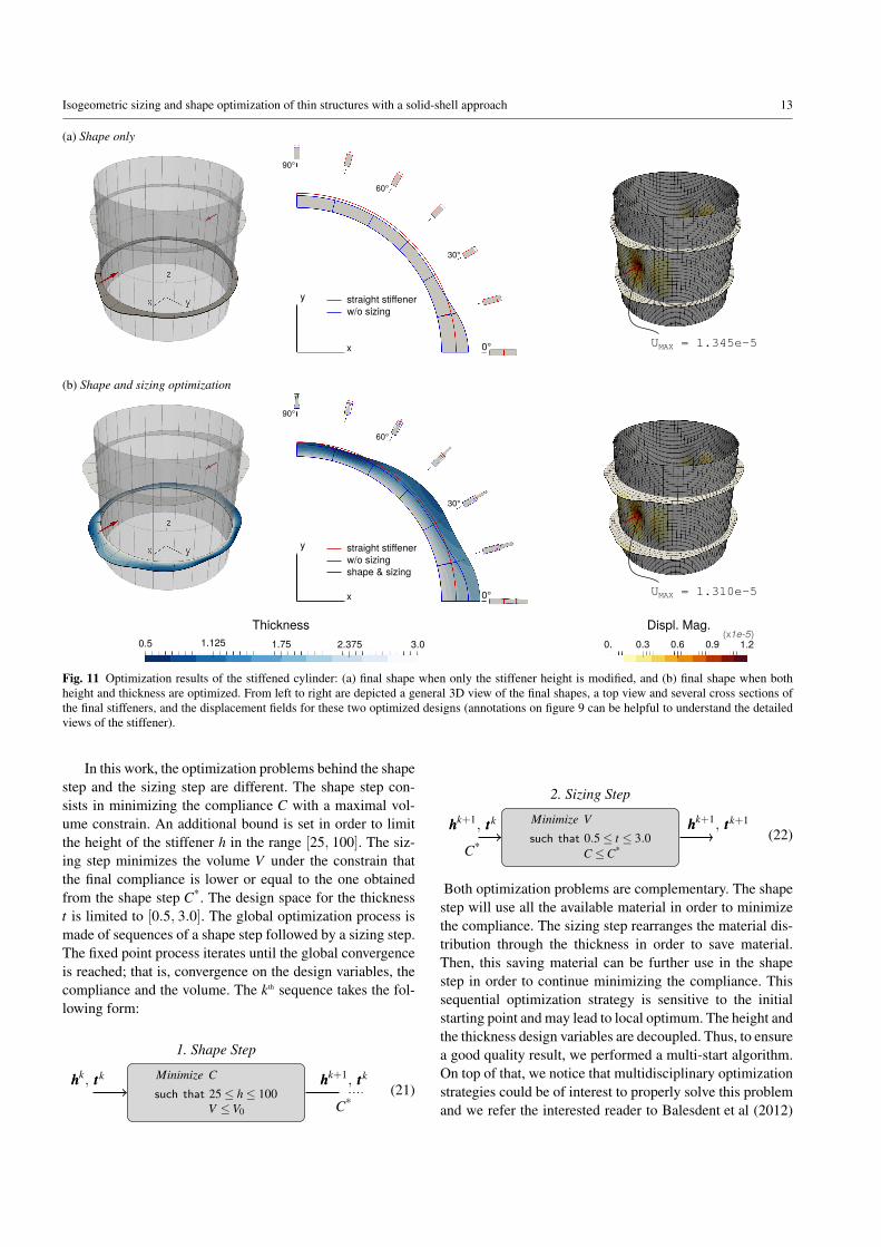
We show the reliability of the procedure on the follow-

ing example. Starting from a roof made of a square plate,

the objective is to optimize the shape and the thickness of

the structure by minimizing the compliance under a maxi-

mal volume constraint. This example is based on the work

of Kegl and Brank (2006) and similar studies can be found

for example in Bletzinger et al (2005); Ikeya et al (2016).

The mechanical parameters of the study are the following:

Young modulus E = 210e9, Poisson ratio ν = 0.30, length

L= 10, thickness h= 0.10, uniform snow load P= 500. The

four corners of the plate are fixed. For the first step, the opti-

mization model is defined by a single quadratic Nurbs patch

which discretize the whole structure in 4-by-4 NURBS ele-

ments. The surface is parametrized with 32 design variables;

the 4 control points located at the corners are kept fixed.

A refinement level of 3 is applied in both parametric direc-

tions, resulting in an analysis model with 1024 quadratic el-

ements. The volume is constrained to be lower than 110%

of the initial volume. Figure 13 shows the final shape. The

SLSQP optimizer converges after approximately 40 itera-

tions. The compliance is drastically reduced with a factor

of 1.44e-03. The final shape has 4 symmetric planes defined

by the origin and the normal vectors X , Y , X+Y and X-Y .

This is expected since the problem presents these symme-

tries. Therefore, some design variables have identical opti-

mal values. The fact that we obtain the symmetries without

setting groups of design variables is a meaningful indication

to validate the result. Moreover, our result is similar to the

one of Kegl and Brank (2006) when the control points are

only modified in Z-direction (case B in section 5.2 of the

cited paper). The optimal positions of the control points are

given on the top view and on the side view of the structure

on figure 13. This global shape could have been obtained us-

ing the solid-shell model as in the previous examples of this

paper.

Once the global shape of the structure is obtained, one

can build a volume model. Here, we create it by offset-

ting the previous surface in Z-direction with a distance of

h = 0.10. This time, only one quarter of the structure is con-

sidered. In order to enrich the design model, knot insertion

is performed. The in-plane parametric directions are defined

by the same knot vector U = 0 0 0 16

26

12

34

1 1 1. Degree

one is chosen in the thickness direction for building the op-

timization model. Thus, the optimization model counts 25

elements. The design variables modify the distance between

the upper and lower surfaces. A total of 36 variables are de-

fined. They parametrize the distance between neighboring

control points of both upper and lower surfaces. The de-

sign variables are bounded so that the distance between the


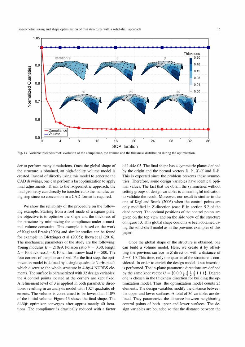
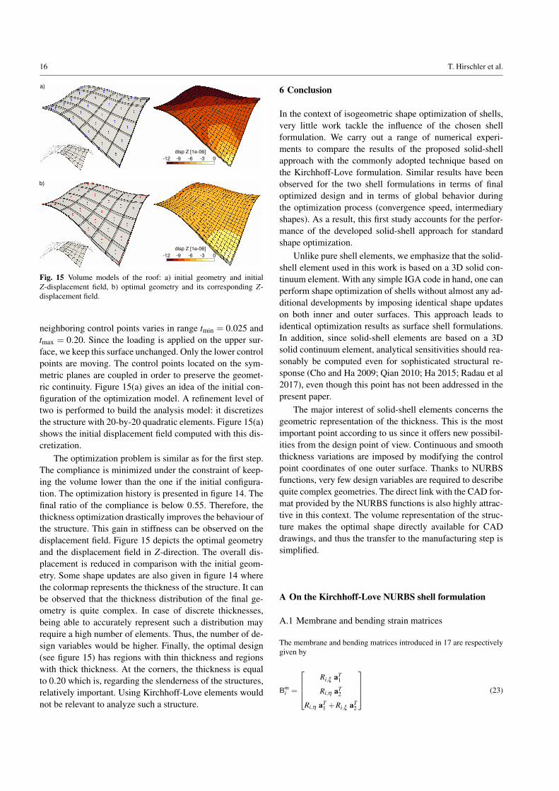
Fig. 15 Volume models of the roof: a) initial geometry and initial

Z-displacement field, b) optimal geometry and its corresponding Z-

displacement field.

neighboring control points varies in range tmin = 0.025 and

tmax = 0.20. Since the loading is applied on the upper sur-

face, we keep this surface unchanged. Only the lower control

points are moving. The control points located on the sym-

metric planes are coupled in order to preserve the geomet-

ric continuity. Figure 15(a) gives an idea of the initial con-

figuration of the optimization model. A refinement level of

two is performed to build the analysis model: it discretizes

the structure with 20-by-20 quadratic elements. Figure 15(a)

shows the initial displacement field computed with this dis-

cretization.

The optimization problem is similar as for the first step.

The compliance is minimized under the constraint of keep-

ing the volume lower than the one if the initial configura-

tion. The optimization history is presented in figure 14. The

final ratio of the compliance is below 0.55. Therefore, the

thickness optimization drastically improves the behaviour of

the structure. This gain in stiffness can be observed on the

displacement field. Figure 15 depicts the optimal geometry

and the displacement field in Z-direction. The overall dis-

placement is reduced in comparison with the initial geom-

etry. Some shape updates are also given in figure 14 where

the colormap represents the thickness of the structure. It can

be observed that the thickness distribution of the final ge-

ometry is quite complex. In case of discrete thicknesses,

being able to accurately represent such a distribution may

require a high number of elements. Thus, the number of de-

sign variables would be higher. Finally, the optimal design

(see figure 15) has regions with thin thickness and regions

with thick thickness. At the corners, the thickness is equal

to 0.20 which is, regarding the slenderness of the structures,

relatively important. Using Kirchhoff-Love elements would

not be relevant to analyze such a structure.

6 Conclusion

In the context of isogeometric shape optimization of shells,

very little work tackle the influence of the chosen shell

formulation. We carry out a range of numerical experi-

ments to compare the results of the proposed solid-shell

approach with the commonly adopted technique based on

the Kirchhoff-Love formulation. Similar results have been

observed for the two shell formulations in terms of final

optimized design and in terms of global behavior during

the optimization process (convergence speed, intermediary

shapes). As a result, this first study accounts for the perfor-

mance of the developed solid-shell approach for standard

shape optimization.

Unlike pure shell elements, we emphasize that the solid-

shell element used in this work is based on a 3D solid con-

tinuum element. With any simple IGA code in hand, one can

perform shape optimization of shells without almost any ad-

ditional developments by imposing identical shape updates

on both inner and outer surfaces. This approach leads to

identical optimization results as surface shell formulations.

In addition, since solid-shell elements are based on a 3D

solid continuum element, analytical sensitivities should rea-

sonably be computed even for sophisticated structural re-

sponse (Cho and Ha 2009; Qian 2010; Ha 2015; Radau et al

2017), even though this point has not been addressed in the

present paper.

The major interest of solid-shell elements concerns the

geometric representation of the thickness. This is the most

important point according to us since it offers new possibil-

ities from the design point of view. Continuous and smooth

thickness variations are imposed by modifying the control

point coordinates of one outer surface. Thanks to NURBS

functions, very few design variables are required to describe

quite complex geometries. The direct link with the CAD for-

mat provided by the NURBS functions is also highly attrac-

tive in this context. The volume representation of the struc-

ture makes the optimal shape directly available for CAD

drawings, and thus the transfer to the manufacturing step is

simplified.

A On the Kirchhoff-Love NURBS shell formulation

A.1 Membrane and bending strain matrices

The membrane and bending matrices introduced in 17 are respectively

given by

Bmi =

Ri,ξ aT1

Ri,η aT2

Ri,η aT1 +Ri,ξ aT

2

(23)


and

Bfi =

Bi1 · e1 Bi

1 · e2 Bi1 · e3

Bi2 · e1 Bi

2 · e2 Bi2 · e3

2Bi3 · e1 2Bi

3 · e2 2Bi3 · e3

. (24)

In 23 and 24, (e1,e2,e3) are the basis vectors of the global Cartesian

coordinates system, and the quantities Bi1, Bi

2 and Bi3 are given by

Bi1 =−Ri,ξ ξ a3 +

1√a

[Ri,ξ a1,ξ ×a2 + Ri,η a1 ×a1,ξ

+ a3 ·a1,ξ

(Ri,ξ a2 ×a3 +Ri,η a3 ×a1

)],

Bi2 =−Ri,ηη a3 +

1√a

[Ri,ξ a2,η ×a2 + Ri,η a1 ×a2,η

+ a3 ·a2,η


)],

Bi3 =−Ri,ξ η a3 +

1√a

[Ri,ξ a1,η ×a2 + Ri,η a1 ×a1,η

+ a3 ·a1,η


)],

(25)

with√

a = |a1 ×a2|.

A.2 Material tensor

The material tensor within the Voigt formalism is in the form

H=E

1−ν2

a11a11 h12 a11a12

∗ a22a22 a22a12

∗ ∗ h33

where: h12 = νa11a22 +(1−ν)a12a12

h33 =12

[(1−ν)a11a22 +(1+ν)a12a12

]

(26)

with E as the Young’s modulus, ν as the Poisson’s ratio, and aαβ =aα · aβ as the contravariant metric. The corresponding contravariant

base vectors aα are defined trough the relation aα · aβ = δαβ where

δαβ is the Kronecker delta.

References

Adams DB, Watson LT, Gurdal Z, Anderson-Cook CM (2004) Genetic

algorithm optimization and blending of composite laminates by lo-

cally reducing laminate thickness. Advances in Engineering Soft-

ware 35(1):35–43

Al Akhras H, Elguedj T, Gravouil A, Rochette M (2017) Towards

an automatic isogeometric analysis suitable trivariate models

generation–Application to geometric parametric analysis. Com-

puter Methods in Applied Mechanics and Engineering 316:623–

645

Apostolatos A, Breitenberger M, Wuchner R, Bletzinger KU (2015)

Domain decomposition methods and kirchhoff-love shell multi-

patch coupling in isogeometric analysis. In: Juttler B, Simeon B

(eds) Isogeometric Analysis and Applications 2014, Springer In-

ternational Publishing, Cham, pp 73–101

Balesdent M, Berend N, Depince P, Chriette A (2012) A survey of

multidisciplinary design optimization methods in launch vehicle

design. Structural and Multidisciplinary Optimization 45(5):619–

642

Bandara K, Cirak F (2017) Isogeometric shape optimisation of shell

structures using multiresolution subdivision surfaces. Computer-

Aided Design

Belytschko T, Stolarski H, Liu WK, Carpenter N, Ong JSJ (1985)

Stress projection for membrane and shear locking in shell finite

elements. Computer Methods in Applied Mechanics and Engineer-

ing 51(1-3):221–258

Benson DJ, Bazilevs Y, Hsu MC, Hughes TJR (2010) Isogeometric

shell analysis: The Reissner-Mindlin shell. Computer Methods in

Applied Mechanics and Engineering 199(5-8):276–289

Bletzinger KU (2014) A consistent frame for sensitivity filtering and

the vertex assigned morphing of optimal shape. Structural and

Multidisciplinary Optimization 49(6):873–895

Bletzinger KU, Wuchner R, Daoud F, Camprubı N (2005) Compu-

tational methods for form finding and optimization of shells and

membranes. Computer Methods in Applied Mechanics and Engi-

neering 194(30-33):3438–3452

Bletzinger KU, Firl M, Linhard J, Wchner R (2010) Optimal shapes of

mechanically motivated surfaces. Computer Methods in Applied

Mechanics and Engineering 199(5):324–333

Bouclier R, Elguedj T, Combescure A (2013) Efficient isogeometric

NURBS-based solid-shell elements: Mixed formulation and B-

method. Computer Methods in Applied Mechanics and Engineer-

ing 267:86–110

Bouclier R, Elguedj T, Combescure A (2015a) Development of a

mixed displacement-stress formulation for the analysis of elasto-

plastic structures under small strains: Application to a locking-

free, NURBS-based solid-shell element. Computer Methods in

Applied Mechanics and Engineering 295:543–561

Bouclier R, Elguedj T, Combescure A (2015b) An isogeometric

locking-free nurbs-based solid-shell element for geometrically

nonlinear analysis. International Journal for Numerical Methods

in Engineering 101(10):774–808

Braibant V, Fleury C (1984) Shape optimal design using b-splines.

Computer Methods in Applied Mechanics and Engineering

44(3):247–267

Cardoso RPR, Cesar De Sa JMA (2014) Blending moving least squares

techniques with NURBS basis functions for nonlinear isogeomet-

ric analysis. Computational Mechanics 53(6):1327–1340

Caseiro JF, Valente RAF, Reali A, Kiendl J, Auricchio F, Alves De

Sousa RJ (2014) On the Assumed Natural Strain method to allevi-

ate locking in solid-shell NURBS-based finite elements. Compu-

tational Mechanics 53(6):1341–1353

Caseiro JF, Valente RAF, Reali A, Kiendl J, Auricchio F, Alves de

Sousa RJ (2015) Assumed natural strain NURBS-based solid-shell

element for the analysis of large deformation elasto-plastic thin-

shell structures. Computer Methods in Applied Mechanics and En-

gineering 284:861–880

Cho S, Ha SH (2009) Isogeometric shape design optimization: ex-

act geometry and enhanced sensitivity. Structural and Multidisci-

plinary Optimization 38(1):53–70

Choi MJ, Cho S (2015) A mesh regularization scheme to update

internal control points for isogeometric shape design optimiza-

tion. Computer Methods in Applied Mechanics and Engineering

285:694–713

Cohen E, Riesenfeld RF, Elber G (2001) Geometric Modeling with

Splines: An Introduction. A. K. Peters, Ltd., Natick, MA, USA

Coox L, Maurin F, Greco F, Deckers E, Vandepitte D, Desmet W

(2017) A flexible approach for coupling nurbs patches in rota-

tionless isogeometric analysis of kirchhofflove shells. Computer

Methods in Applied Mechanics and Engineering 325:505 – 531


Cottrell JA, Hughes TJR, Bazilevs Y (2009) Isogeometric Analysis:

Toward Integration of CAD and FEA, 1st edn. Wiley Publishing

Daxini SD, Prajapati JM (2017) Parametric shape optimization tech-

niques based on Meshless methods: A review. Structural and Mul-

tidisciplinary Optimization 56(5):1197–1214

Ding CS, Cui XY, Li GY (2016) Accurate analysis and thickness op-

timization of tailor rolled blanks based on isogeometric analysis.

Structural and Multidisciplinary Optimization 54(4):871–887

Dornisch W, Klinkel S, Simeon B (2013) Isogeometric Reissner-

Mindlin shell analysis with exactly calculated director vec-

tors. Computer Methods in Applied Mechanics and Engineering

253:491–504

Duong TX, Roohbakhshan F, Sauer RA (2017) A new rotation-free

isogeometric thin shell formulation and a corresponding continu-

ity constraint for patch boundaries. Computer Methods in Applied

Mechanics and Engineering 316:43–83

Echter R, Oesterle B, Bischoff M (2013) A hierarchic family of isoge-

ometric shell finite elements. Computer Methods in Applied Me-

chanics and Engineering 254:170–180

Farin G (2002) Curves and Surfaces for CAGD: A Practical Guide, 5th

edn. Morgan Kaufmann Publishers Inc., San Francisco, CA, USA

Firl M, Wuchner R, Bletzinger KU (2013) Regularization of shape

optimization problems using FE-based parametrization. Structural

and Multidisciplinary Optimization 47(4):507–521

Fußeder D, Simeon B, Vuong AV (2015) Fundamental aspects of shape

optimization in the context of isogeometric analysis. Computer

Methods in Applied Mechanics and Engineering 286:313–331

Goyal A, Simeon B (2017) On penalty-free formulations for multipatch

isogeometric KirchhoffLove shells. Mathematics and Computers

in Simulation 136:78–103

Guo Y, Ruess M, Schillinger D (2017) A parameter-free variational

coupling approach for trimmed isogeometric thin shells. Compu-

tational Mechanics 59(4):693–715

Ha YD (2015) Generalized isogeometric shape sensitivity analy-

sis in curvilinear coordinate system and shape optimization of

shell structures. Structural and Multidisciplinary Optimization

52(6):1069–1088

Herrema AJ, Wiese NM, Darling CN, Ganapathysubramanian B, Kr-

ishnamurthy A, Hsu MC (2017) A framework for parametric de-

sign optimization using isogeometric analysis. Computer Methods

in Applied Mechanics and Engineering 316:944–965

Hirt G, Senge S (2014) Selected Processes and Modeling Techniques

for Rolled Products. Procedia Engineering 81(October):18–27

Hughes TJR, Cottrell JA, Bazilevs Y (2005) Isogeometric analysis:

CAD, finite elements, NURBS, exact geometry and mesh refine-

ment. Computer Methods in Applied Mechanics and Engineering

194(39-41):4135–4195

Ikeya K, Shimoda M, Shi JX (2016) Multi-objective free-form opti-

mization for shape and thickness of shell structures with compos-

ite materials. Composite Structures 135:262–275

Imam MH (1982) Three-dimensional shape optimization. International

Journal for Numerical Methods in Engineering 18(5):661–673

Jones E, Oliphant T, Peterson P, et al (2001–) SciPy: Open source sci-

entific tools for Python. URL http://www.scipy.org/

Kang P, Youn SK (2016) Isogeometric shape optimization of trimmed

shell structures. Structural and Multidisciplinary Optimization

53(4):825–845

Kegl M, Brank B (2006) Shape optimization of truss-stiffened shell

structures with variable thickness. Computer Methods in Applied

Mechanics and Engineering 195(19-22):2611–2634

Kiendl J, Bletzinger KU, Linhard J, Wchner R (2009) Isogeometric

shell analysis with Kirchhoff-Love elements. Computer Methods

in Applied Mechanics and Engineering 198(49-52):3902–3914

Kiendl J, Bazilevs Y, Hsu MC, Wuchner R, Bletzinger KU (2010) The

bending strip method for isogeometric analysis of Kirchhoff-Love

shell structures comprised of multiple patches. Computer Methods

in Applied Mechanics and Engineering 199(37-40):2403–2416

Kiendl J, Schmidt R, Wuchner R, Bletzinger KU (2014) Isogeomet-

ric shape optimization of shells using semi-analytical sensitivity

analysis and sensitivity weighting. Computer Methods in Applied

Mechanics and Engineering 274:148–167

Kopp R, Wiedner C, Meyer A (2005) Flexibly Rolled Sheet Metal and

its use in Sheet Metal Forming. Advanced Materials Research 6-

8:81–92

Kraft D (1988) A Software Package for Sequential Quadratic Pro-

gramming. Deutsche Forschungs- und Versuchsanstalt fur Luft-

und Raumfahrt Koln: Forschungsbericht, Wiss. Berichtswesen d.

DFVLR

Lam YC, Manickarajah D, Bertolini A (2000) Performance charac-

teristics of resizing algorithms for thickness optimization of plate

structures. Finite elements in analysis and design 34(2):159–174

Le C, Bruns T, Tortorelli D (2011) A gradient-based, parameter-free

approach to shape optimization. Computer Methods in Applied


Lee BG, Park Y (2002) Degree elevation of nurbs curves by weighted

blossom. Korean Journal of Computational & Applied Mathemat-

ics 9(1):151–165

Lee S, Hinton E (2000) Dangers inherited in shells optimized with lin-

ear assumptions. Computers and Structures 78(1):473–486

Liu L, Zhang Y, Hughes TJR, Scott MA, Sederberg TW (2014) Volu-

metric T-spline construction using Boolean operations. Engineer-

ing with Computers 30(4):425–439

Lund E (1994) Finite element based design sensitivity analysis and

optimization. PhD thesis, Aalborg University

Martins JRRA, Lambe AB (2013) Multidisciplinary Design Optimiza-

tion: A Survey of Architectures. AIAA Journal 51(9):2049–2075

Merklein M, Johannes M, Lechner M, Kuppert A (2014) A review on

tailored blanks–Production, applications and evaluation. Journal

of Materials Processing Technology 214(2):151–164

Nagy AP, Abdalla MM, Gurdal Z (2010) Isogeometric sizing and shape

optimisation of beam structures. Computer Methods in Applied


Nagy AP, Abdalla MM, Gurdal Z (2011) Isogeometric design of elastic

arches for maximum fundamental frequency. Structural and Mul-

tidisciplinary Optimization 43(1):135–149

Nagy AP, Ijsselmuiden ST, Abdalla MM (2013) Isogeometric design of

anisotropic shells: Optimal form and material distribution. Com-

puter Methods in Applied Mechanics and Engineering 264:145–

162

Nguyen DM, Evgrafov A, Gravesen J (2012) Isogeometric Shape Op-

timization for Electromagnetic Scattering Problems. Progress In

Electromagnetics Research B 45:117–146

Nha CD, Xie Y, Steven G (1998) An evolutionary structural optimiza-

tion method for sizing problems with discrete design variables.

Computers & Structures 68(4):419–431

Piegl L, Tiller W (1997) The NURBS Book (2Nd Ed.). Springer-Verlag

New York, Inc., New York, NY, USA

Qian X (2010) Full analytical sensitivities in NURBS based isogeomet-

ric shape optimization. Computer Methods in Applied Mechanics

and Engineering 199(29-32):2059–2071

Radau L, Gerzen N, Barthold FJ (2017) Sensitivity of structural re-

sponse in context of linear and non-linear buckling analysis with

solid shell finite elements. Structural and Multidisciplinary Opti-

mization 55(6):2259–2283

Ramm E, Bletzinger KU, Reitinger R (1993) Shape optimization of

shell structures. Revue Europenne des lments Finis 2(3):377–398

Taheri A, Hassani B (2014) Simultaneous isogeometrical shape and

material design of functionally graded structures for optimal

eigenfrequencies. Computer Methods in Applied Mechanics and

Engineering 277:46 – 80

Wall WA, Frenzel MA, Cyron C (2008) Isogeometric structural shape

optimization. Computer Methods in Applied Mechanics and Engi-

http://www.scipy.org/


neering 197(33-40):2976–2988

Wang ZP, Turteltaub S (2015) Isogeometric shape optimization for

quasi-static processes. International Journal for Numerical Meth-

ods in Engineering 104(5):347–371

Wang ZP, Abdalla M, Turteltaub S (2017a) Normalization approaches

for the descent search direction in isogeometric shape optimiza-

tion. CAD Computer Aided Design 82(June):68–78

Wang ZP, Poh LH, Dirrenberger J, Zhu Y, Forest S (2017b) Isoge-

ometric shape optimization of smoothed petal auxetic structures

via computational periodic homogenization. Computer Methods

in Applied Mechanics and Engineering 323:250–271

Wang ZP, Turteltaub S, Abdalla M (2017c) Shape optimization and

optimal control for transient heat conduction problems using an

isogeometric approach. Computers and Structures 185:59–74

Documents

Isogeometric sizing and shape optimization of thin