Isoefficiency : Measuring the Scalability of Parallel Algorithms and Architectures Ananth Y. Grama, Anshul Gupta, and Vipin Kumar University of Minnesota

Isoeffiency analysis helps us determine the best akorith m/a rch itecture combination for a particular p ro blem without explicitly analyzing all possible combinations under all possible conditions.

An earlier version of this article appeared as “Analyzing Performance of Large-scale Parallel Systems” by Anshul Gupta and Vipin Kumar on pp. 144-153 of the Proceedings ofthe 26th Hawaii International Confwence MI System Sciences, published in 1993 by IEEE Computer Society Press, Los Alamitos, Calif.

T he fastest sequential algorithm for a given problem is the best sequential algorithm. But determining the best par- allel algorithm is considerably more complicated. A par- allel algorithm that solves a problem well using a fixed number of processors on a particular architecture may

perform poorly if either of these parameters changes. Analyzing the per- formance of a given parallel algorithdarchitecture calls for a compre- hensive method that accounts for scalability: the system’s ability to increase speedup as the number of processors increases.

The isoefficiency function is one of many parallel performance met- rics that measure It relates problem size to the number of processors required to maintain a system’s efficiency, and it lets us deter- mine scalability with respect to the number of processors, their speed, and the communication bandwidth of the interconnection network. The isoefficiency function also succinctly captures the characteristics of a par- ticular algorithdarchitecture combination in a single expression, letting us compare various combinations for a range of problem sizes and num- bers of processors. Thus, we can determine the best combination for a problem without explicitly analyzing all possible combinations under all possible conditions. (The sidebar on page 14 defines many basic concepts of scalability analysis and presents an example that is revisited through- out the article.)

12 1063-6SS2/93/0800-0012 $3.000 1993 IEEE IEEE Parallel & Distributed Technology

Scalable parallel systems The number of processors limits a par- allel system's speedup: The speedup for a single processor is one, but if more are used, the speedup is usually less than the number of processors.

Let's again consider the example in the sidebar. Figure 1 shows the speedup for a few values of n on up to 3 2 proces- sors; Table 1 shows the corresponding efficiencies. The speedup does not increase linearly with the number of

6? 10 'T

igure 1. Speedup versus number of processors for adding a l i s t of numbers on a hypercube.

processors; instead, it tends to saturate. In other words, the efficiency drops as the number of processors increases. Tlus is true for all parallel systems, and is often referred to as Amdahl's law. But the figure and table also show a higher speedup (efficiency) as the problem size increases on the same number of processors.

If increasing the number of processors reduces effi- ciency, and increasing the problem size increases effi- ciency, we should be able to keep efficiency constant by increasing both simultaneously. For example, the table shows that the efficiency of adding 64 numbers on a four-processor hypercube is 0.80. When we increase p to eight and n to 192, the efficiency remains 0.80, as it does when we further increase p to 16 and n to 512. Many parallel systems behave in this way. We call them scalable parallel systems.

The isoefficiency function A natural question at this point is: At what rate should we increase the problem size with respect to the num- ber of processors to keep the efficiency fixed? The answer varies depending on the system.

In the sidebar, we noted that the sequential execution time T, equals the problem size Wmultiplied by the cost of executing each operation (t,). Making this sub- stitution in the efficiency equation gives us

If the problem size Wis constant while p increases, then the efficiency decreases because the total overhead T, increases with p . If Wincreases while p is constant, then, for scalable parallel systems, the efficiency increas- es because To grows slower than @(w) (that is, slower than all functions with the same growth rate as LV). We can maintain the efficiency for these parallel systems at

Table 1. Efficiency as a function of n and p for adding n numbers on p-processor hypercubes.

n = 64 1.0 3 0 .57 .33 .17

n=320 1.0 .95 .87 .71 .50 n=512 1.0 .97 .91 .80 .62

n = 192 1.0 .92 .80 .60 .38

a desired value (between 0 and 1) by increasingp, pro- vided W also increases. For different parallel systems, we must increase Wat different rates with respect top to maintain a fixed efficiency. For example, W might need to grow as an exponential function ofp. Such sys- tems are poorly scalable: It is difficult to obtain good speedups for a large number of processors on such sys- tems unless the problem size is enormous. On the other hand, if Wneeds to grow only linearly with respect to p , then the system is highly scalable: Its speedups increase linearly with respect to the number of proces- sors for problem sizes increasing at reasonable rates.

For scalable parallel systems, we can maintain effi- ciency at a desired value (0 < E < 1) if T,/Wis constant:

w='(").. t r 1 - E

If K = E/(t,( 1 - E ) ) is a constant that depends on the efficiency, then we can reduce the last equation to

W = KT,

August 1993 13

Through algebraic manipulations, we can use this equation to obtain Was a function ofp. This function dictates how Wmust grow to maintain a fixed efficien- cy as p increases. This is the system’s isoeficienqificnc- tion. It determines the ease with which the system yields speedup in proportion to the number of processors. A small isoefficiency function implies that small incre- ments in the problem size are sufficient to use an increasing number of processors efficiently; hence, the system is highly scalable. Conversely, a large isoeffi- ciency function indicates a poorly scalable parallel sys- tem. Furthermore, the isoefficiency function does not exist for some parallel systems, because their efficiency cannot be kept constant as p increases, no matter how fast the problem size increases.

For the equation above, if we substitute the value of T, from the example in the sidebar, we get W = 2 Kp log p . Thus, this system’s isoefficiency function is @( p log p) . If the number of processors increases from p top’, the problem size (in this case n) must increase by a factor of (p’ logp’)/( p logp) to maintain the same effi- ciency. In other words, increasing the number of proces-

sors by a factor of p’/p requires n to be increased by a factor of (p’ logp’)/(p logp) to increase the speedup by a factor ofp‘/p.

In this simple example of adding n numbers, the com- munication overhead is a function of onlyp. But a typ- ical overhead function can have several terms of differ- ent orders of magnitude with respect to both the problem size and the number of processors, making it impossible (or a t least cumbersome) to obtain the iso- efficiency function as a closed form function ofp.

Consider a parallel system for which T - - p3/2 +p3/4w3/4

The equation W = KT, becomes W = Kp3/2 + Kp3/4W3/4

For this system, it is difficult to solve for Win terms of p . However, since the condition for constant efficiency is that the ratio of T, and Wremains fixed, then ifp and Wincrease, the efficiency will not drop if none of the terms of T, grows faster than W. W e thus balance each term of T, against Wto compute the corresponding iso-

14 IEEE Parallel & Distributed Technology

3 7 11 15 2 6 10 14 1 5 9 1 3 0 4 8 1 2

~- ~~~~ ___

efficiency function. The term that causes the problem size to grow fastest with respect top determines the sys- tem’s overall isoefficiency function. Solving for the first term in the above equation gives us

Solving for the second term gives us W = Kp3/4W3/4 Wv4 = Kp3/4

W = K4p3 = 0 ( p 3 )

So if the problem size grows as 0 ( p 3 / ’ ) and @ ( p 3 ) , respectively, for the first two terms of T,, then efficien- cy will not decrease as p increases The isoefficiency function for this system is therefore O(p3), which is the higher rate. If Wgrows as 0 ( p 3 ) , then T, will remain of the same order as W.

OFTIMUKNG COST A parallel system is cost-optimal if the product of the number of processors and the parallel execution time is

proportional to the execution time of the best serial algorithm on a single processor:

In the sidebar, we noted that pTp = TI + T,, so

T I + T , = W

Since TI = Wt,, we have

wt,+T,- w W- T,

This suggests that a parallel system is cost-optimal if its overhead function and the problem size are of the same order of magnitude. This is exactly the condition required to maintain a fixed efficiency while increasing the number of processors. So, conforming to the isoef- ficiency relation between Wand p keeps a parallel sys- tem cost-optimal as it is scaled up.

How small can an isoefficiency function be, and what is an ideally scalable parallel system? If a problem con-

August 1993 15

sists of Wbasic operations, then a cost-optimal system can use no more than Wprocessors. If the problem size grows a t a rate slower than @ ( p ) as the number of processors increases, then the number of processors will eventually exceed W. Even in an ideal parallel system with no communication or other overhead, the effi- ciency will drop because the processors exceeding W will have no work to do. So, the problem size has to increase a t least as fast as @ ( p ) to maintain a constant efficiency; hence @ ( p ) is the lower bound on the isoef- ficiency function. It follows that the isoefficiency func- tion of an ideally scalable parallel system is @ ( p ) .

DEGREE OF CONCURRENCY The lower bound of @ ( p ) is imposed on the isoeffi- ciency function by the algorithm's degree of commen- cy: the maximum number of tasks that can be execut- ed simultaneously in a problem of size W. This measure is independent of the architecture. If C( W ) is an algorithm's degree of concurrency, then given a problem of size W, at most C( W ) processors can be employed effectively. For example, using Gaussian elimination to solve a system of n equations with n vari- ables, the total amount of computation is @(1z3). How- ever, the n variables have to be eliminated one after the other, and eliminating each variable requires @(n')

Vector

computations. Thus, at most @(n') processors can be kept busy at a time.

Now if W = @(n3) for this problem, then the degree of concurrency is @(W2'j). Given a problem of size W, at most @(W?/') processors can be used, so given p processors, the size of the problem should be at least @( p3'?) in order to use all the processors. Thus, the iso- efficiency function of this computation due to concur- rency is @( p 3 l 2 ) .

The isoefficiency function due to concurrency is opti- mal - @ ( p ) - only if the algorithm's degree of con- currency is @( W). If it is less than @( W), then the iso- efficiency function due to concurrency is worse (greater) than @ ( p ) . In such cases, the system's overall isoeffi- ciency function is the maximum of the isoefficiency functions due to concurrency, communication, and other overhead.

Isoefficiency analysis Isoefficiency analysis lets us test a program's perfor- mance on a few processors and then predict its perfor- mance on a larger number of processors. It also lets us study system behavior when other hardware parame- ters change, such as processor and communication speeds.

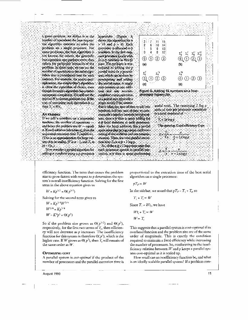
Figure 2. Multiplication of an n x n matrix with an n x 1 vector using "rowwise" striped data partitioning.

COMPARING ALGORITHMS W e often must compare the perfor- mance of two parallel algorithms for a large number of processors. The iso- efficiency function gives us the tool to do so. The algorithm with the small- er isoefficiency function ylelds better performance as the number of proces- sors increases.

Consider the problem of multiply- ing an i z x n matrix with an n x 1 vec- tor. The number of basic operations (the problem size ur) for this matrix- vector product is n?. If the time taken by a single addition and multiplication operation together is t,, then the sequential execution time of this algo- rithm is rz't, (that is, TI = n2t,).

Figure 2 illustrates a parallel version of this algorithm based on a striped partitioning of the matrix and the vec- tor. Each processor is assigned n/p rows of the matrix and n/p elements of

16 IEEE Parallel & Distributed Technology

the vector. Since the multiplication requires the vector to be multiplied with each row of the matrix, every processor needs the entire vector. T o accomplish this, each processor broad- casts its n/p elements of the vector to every other processor (this is called an all-to-allbroahrt). Each processor then has the vector available locally and n/p rows of the matrix. Using these, it com- putes the dot products locally, gwing it n/p elements of the resulting vector.

Let's now analyze this algorithm on a hypercube. The all-to-all broadcast can be performed in ts logp + twn(pl)/p (t, is the startup time of the communi-

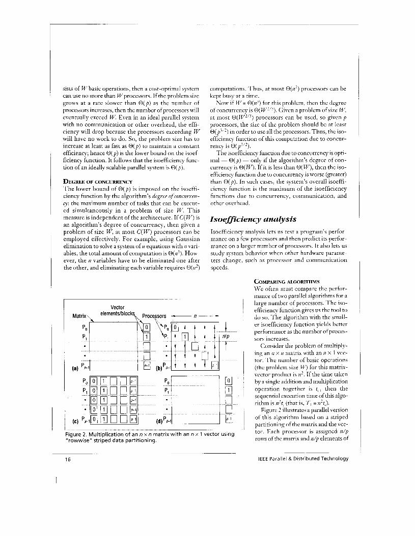
Figure 3. Matrix-vector multiplication using checkerboard partitioning.

cation network, and tw is the per-word transfer time).7 For large values of p we can approximate this as ts log p + twn. Assuming that an additiodmultiplication pair takes tcunits of time, each processor spends tcn2/p units of time in multiplying its n/p rows with the vector. Thus, the parallel execution time of this procedure is

Tp = tc(n2/p) + t, logp + t,n

The speedup and efficiency are

P S = 1 + P(t,l%P+twn) t,n'

Using the relation T, =pTp- TI, the total overhead is

To = tsp logp + twnp

Now we can determine the isoefficiency function. Rewriting the equation W= Do using only the first term of T, gives the isoefficiency term due to the message startup time:

W = Ktsp logp

Similarly, we can balance the second term of T, (due to per-word transfer time) against the problem size W:

n2 = Ktwnp

n = Kt,p

W = a2 = K2tw2p2

From the equations for both terms, we can infer that the problem size needs to increase with the number of

processors at an overall rate of Ob2) to maintain a fixed efficiency.

Another example Now instead of partitioning the matrix into stripes, let's use Checkerboard partitioning: divide it into p squares, each of dimensions (n/$) x (n/$).7 Figure 3 shows the algorithm.

The vector is distributed along the last column of the mesh. In the first step, all processors of the last column send their n/$elements of the vector to the diagonal processor of their respective rows (Figure 3a). Then the

erform a columnwise one-to-all broadcast processo? of the n/ p elements (Figure 3b). The vector is then aligned along the rows of the matrix. Each processor er-

of products. Each processor now has n/$partial sums that need to be accumulated along each row to obtain the product vector (Figure 3c). The last step is a single-node accumulation of the n/$values in each row, with the last processor of the row as the destination (Figure 3d).

On a hypercube with store-and-forward routing, the first step can be performed in at most ts + t,(n/$) log $ time.7 The second step can be performed in (t, + t,n/$) log $time. If a multiplication and an addition are assumed to take tc units of time, then each processor spends about tcn2/p time performing computation. If the product vector must be placed in the last column (like the starting vector), then a single-node accumulation of vector components of size n/$must be performed in each row. Ignoring the time needed to perform addi- tions during this step, the accumulation can be per- formed with a communication time of (ts + t&$) log $. The total parallel execution time is

forms n2/p multiplications and locally adds the n/ P p sets

August 1993 17

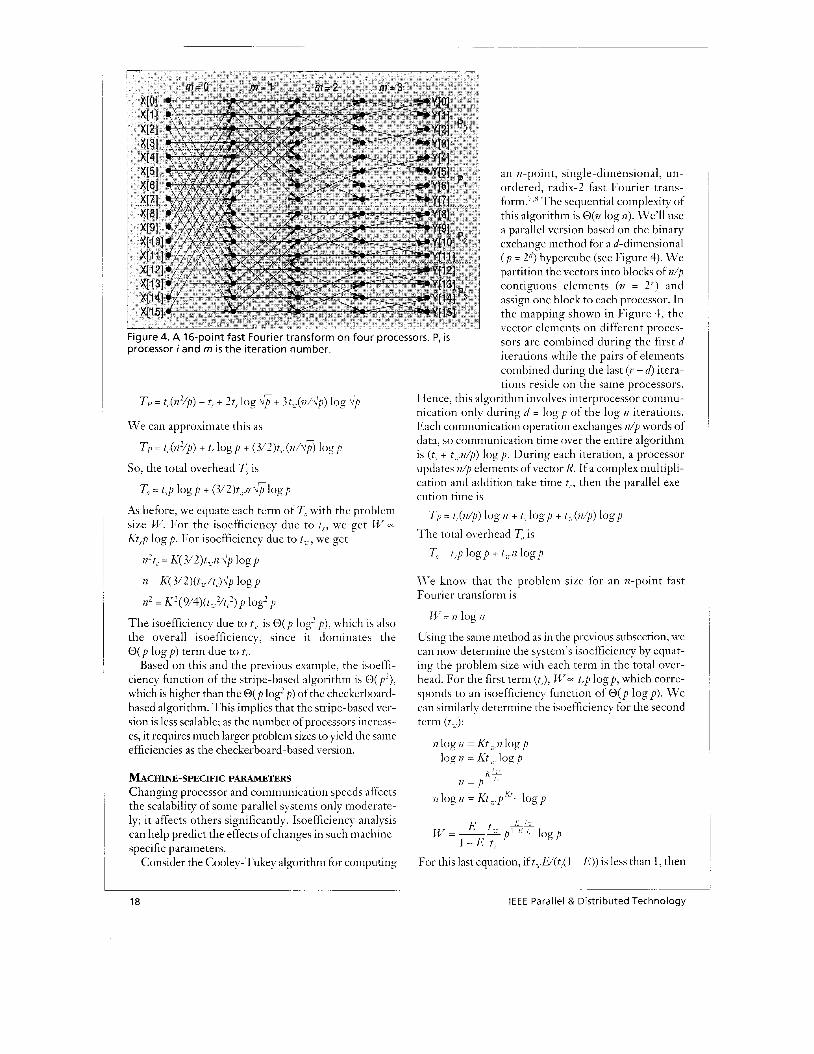
Figure 4. A 16-point fast Fourier transform on four processors. Pi i s processor i and m is the iteration number.

Tp = t,(n'/p) + t, + 2tJ log $+ 3t,.(12/43 log dF We can approximate this as

TI, = t , (d/p) + t, logp + ( 3 / 2 ) t 7 r ( ~ ~ / d 3 logp

So, the total overhead To is

To = t.p logp + (3/2)t,.17 dT10gp

As before, we equate each term of TI with the problem size W. For the isoefficiency due to t,, we get W - Kt,p logp. For isoefficiency due to t::, we get

I z ' t , = K( 3/2)t,.n dF10gp

72 = K( 3/2)(t,./t,)$logp

72' = K'( 9/4)(ti:.'/tL.') p log' p The isoefficiency due to t,. is O ( p log? p ) , which is also the overall isoefficiency, since it dominates the O( p log p ) term due to t3..

Based on this and the previous example, the isoeffi- ciency function of the stripe-based algorithm is O(p') , which is higher than the O( p log2 p) of the checkerhoard- based algorithm. This implies that the stripe-based ver- sion is less scalable; as the number of processors increas- es, it requires much larger problem sizes to yield the same efficiencies as the checkerboard-based version.

MACHINE-SPECIFIC PARAMETERS Changing processor and communication speeds affects the scalability of some parallel systems only moderate- ly; it affects others significantly. Isoefficiency analysis can help predict the effects of changes in such niachine- specific parameters.

Consider the Cooley-Tukey algorithm for computing

~

18

an 17 -point, single -di mensional , u n- ordered, radix-2 fast Fourier trans- form.:,' The sequential complexity of this algorithm is O(n log 72). We'll use a parallel version based on the binary exchange method for a &dimensional ( p = 2n) hypercube (see Figure 4). W e partition the vectors into blocks of n/p contiguous elements (n = 2'-) and assign one block to each processor. In the mapping shown in Figure 4, the vector elements on different proces- sors are combined during the first d iterations while the pairs of elements combined during the last ( T - - d) itera- tions reside on the same processors.

Hence, this algorithm involves interprocessor commu- nication only during d = log p of the log 17 iterations. Each communication operation exchanges w'p words of data, so communication titne over the entire algorithm is (t,< + t;&) log p. During each iteration, a processor updates 77/p elements of vector R. If a complex multipli- cation and addition take time t(., then the parallel exe- cution time is

Tp = t , ( 7 7 / " ) log I7 + t, log^ + t::.(11/p) logp The total overhead TI is

7;) = t3p logp + t ; : . /1 logp

IZ'e know that the problem size for an n-point fast Fourier transform is

rz/ = log 7z

Using the same method as in the previous subsection, we can now determine the system's isoefficiency by equat- ing the problem size with each term in the total over- head. For the first term (t,J, W- tJp logp, which corre- sponds to an isoefficiency function of O( p log p ) . W e can similarly determine the isoefficiency for the second term (t:?):

For this last equation, if t7JZ/(tc.( I - E ) ) is less than 1, then

-~ ~~~~

IEEE Parallel & Distributed Technology

Ws rate of growth is less than O(p logp), so the overall isoefficiency function is O( p logp). But if t,E/(tc( 1 - E)) is greater than 1, then the overall isoefficiency function is greater than O( p log p ) . The isoefficiency function depends on the relative values of E/(1 - E) , t,, and t,. Thus, this algorithm is unique in that the isoefficiency function is a function not only of the desired efficiency, but also of the hardware-dependent parameters. In fact, the efficiency corresponding to t,E/(tc( 1 - E)) = 1 - that is, U(1 - E ) = t&,, or E = t,/(tc + t,) - acts as a thresh- old value for efficiency. For a hypercube, efficiencies up to this value can be obtained easily. But much higher efficiencies can be obtained only if the problem size is extremely large.

Let’s examine the effect of the value of t,E/(tc( 1 - E ) ) on the iso- efficiency function. If t, = t,, then the isoefficiency function is E/( 1 - E)pE’(’ - log p . Now for E/(l - E ) I 1 (that is, E 5 O.S), the overall isoefficiency is O ( p logp), but for E > 0.5 it is much worse. For instance, if E = 0.9, then E/( 1 - E ) = 9 and the isoefficiency function is O( p9 log p). Now if t, = 2tc and the threshold efficiency is 0.3 3 , then the isoefficiency func- tion for E = 0.3 3 is O( p log. p ) , for

Consider Dijkstra’s all-pairs shortest-path problem for a dense graph with n ~ertices.’,~ The problem involves finding the shortest path between each pair of vertices. The best-known serial algorithm takes O(n3) time. We can also solve this problem by executing one instance of the single-source shortest-path algorithm for each of the n vertices. The latter algorithm deter- mines the shortest path from one vertex to every other vertex in the graph. Its sequential complexity is O(n2).

We can derive a simple parallel version of this algo- rithm by executing a single-source

Some parallel algorithms that seem attractive because of their low overhead have limited concurrency, making them perform poorly as the number of processors grows. IsoeMciency analysis can capture this effect.

E = 0.5 it is 0(p2 log);), anYd for E = 0.9 it is O(p18 logp).

These examples show that the efficiency we can obtain for reasonable problem sizes is limited by the ratio of the CPU speed to the hypercube’s communication band- width. We can raise this limit by increasing the band- width, but making the CPU faster without improving the bandwidth lowers this threshold. In other words, this algo- rithm performs poorly on a hypercube whose communi- cation and computation speeds are not balanced. How- ever, the algorithm is fairly scalable on a balanced hypercube with an overall isoefficiency function of O( p logp), and good efficiencies can be expected for a rea- sonably large number of processors.

CONCURRENCY Some parallel algorithms that seem attractive because of their low overhead have limited concurrency, mahng them perform poorly as the number of processors grows. Isoefficiency analysis can capture this effect.

- - shortest-path problem indepen- dently on each of n processors. Since each of these computations is independent of the others, the parallel algorithm requires no communication, mahng it seem that it is the best possible algo- rithm. But the algorithm can use at most n processors ( p = n), and since the problem size Wis @(a3), Wmust grow at least as O(p3) to use more processors. So the over- all isoefficiency is relatively high; other algorithms with better iso- efficiencies are available.

CONTENTION FOR SHARED DATA STRUCruRES An algorithm can have low com- - munication overhead and high concurrency, but still have over-

head from contention over shared data structures. Such overhead is difficult to model, malung it difficult to com- pute the parallel execution time. However, we can still use isoefficiency analysis to determine the scalability.

Consider an application that solves discrete opti- mization problems by performing a depth-first search of large unstructured trees. Some parallel algorithms solve this problem by using a dynamic load-balancing strategy. ‘OJ’ All work is initially assigned to one proces- sor. An idle processor Pi selects a processor P, using some selection criterion and sends it a work request. If processor P, has no work, it responds with a reject mes- sage; otherwise, it partitions its work into two parts and sends one part to Pi (as long as the work is larger than some minimum size). This process continues until all processors exhaust the available work.

One selection criterion -global round robin - main- tains a global pointer G at one of the processors. This

August 1993 19

pointer initially points to the first processor. When an idle processor needs to select Pa, it reads the current value of G, and requests work from Pc. The pointer is incremented by one (modulo p) before the next request is processed. The pointer distributes the work requests evenly over the processors.

The nondeterministic nature of this algorithm makes it impossible to estimate the exact parallel execution time beforehand. We can, however, set an upper bound on the communication COS^.'^^^ Under certain assump- tions,1° the upper bound on the number of communi- cations is O( p log W ) (that is, it is of the same order or smaller than p log W ) . If each communication takes O(1ogp) time, then the total overhead from the com- munication of work is bounded by O( p logp log W). As before, we can equate this term with the problem size to derive the isoefficiency due to communication overhead:

W.. O(p logp log W )

If we take the Won the right hand side of this expres- sion, put the value of Win its place, and ignore the dou- ble log terms, then the isoefficiency due to communi- cation overhead is O(p log2 p).

But &s term does not specify the system’s overall iso- efficiency because the algorithm also has overhead due to contention: Only one processor can access the glob- al variable at a time; others must wait. So, we must also analyze the system’s isoefficiency due to contention.

The global variable is accessed a total of O(p log W ) times (for the read and increment operations). If the processors are used efficiently, then the total execution time is O(W/p). If there is no contention while solving a problem of size Wonp processors, then W/p is much greater than the total time during whch the shared vari- able is accessed. Now, as we increase the number of processors, the total execution time (W/p) decreases, but the number of times the shared variable is accessed increases. At some point, the shared variable access becomes a bottleneck, and the overall execution time cannot be reduced further. We can eliminate this bot- tleneck by increasing W at a rate such that the ratio between W/p and O ( p log W ) remains the same. Equating W/p and O(p log W ) and then simplifying yields an isoefficiency of O( p 2 log p ) . Thus, since the isoefficiency due to contention dominates the isoeffi- ciency due to communication, the overall isoefficiency is O(p2 logp). (It has been shown elsewhere that dynam- ic load-balancing schemes with better isoefficiency functions outperform those with poorer isoefficiency functions. lo)

20

T he isoefficiency metric is useful when we want performance to increase at a linear rate with the number of processors: If the problem size grows at the rate spec- ified by the isoefficiency function, then

the system’s speedup is linear. In some cases, though, we might not want (or be able) to increase the problem size at the rate specified by the isoefficiency function; if the problem size grows at a smaller rate, then the speedup is sublinear.

For a grven growth rate, we can use the speedup curve as a scalability metric. If the problem size increases at a linear rate with the number of processors, the curve shows scaled speedup.2 The growth rate can also be con- strained by the computer’s memory, in which case the problem size increases at the fastest rate allowed by the available m e m ~ r y . ~ ~ ~ , ~

In many situations, the growth rate is dictated by the time available to solve the problem, in which case the problem size increases with the number of processors in such a way that the run time remains ~ o n s t a n t . ~ , ~ , ~ W e can also keep the problem size fixed and use the speedup curve as a scalability metric.12

There are interesting relationships between isoeffi- ciency and some of these metrics. If the isoefficiency function is greater than O(p), then the problem size for a scalable parallel system cannot increase indefinitely while maintaining a fixed execution time, no matter how many processors are used.’J2 Also, for a class of paral- lel systems, the isoefficiency function specifies the rela- tionship between the problem size’s growth rate and the number of processors on which the problem executes in minimum time.12

ACKNOWLEDGMENTS This work was supported by Army Research Office grant 28408-MA- SDI to the University of Minnesota, and by the Army High Perfor- mance Computing Research Center at the University of Minnesota. We also thank Daniel Challou and Tom Nurkkala for their help in preparing this article.

REFERENCES 1. V. Kumar and A. Gupta, “Analyzing Scalability of Parallel Algo-

rithms and Architectures,” Tech. Report 91-18, Computer Sci- ence Dept., Univ. of Minnesota, Minneapolis, 1991.

2. J.L. Gustafson, “Reevaluating Amdahl’s Law,” Cmm. ACM, Vol. 31, NO. 5 , 1988, pp. 532-533.

3. J.L. Gustafson, “The Consequences of Fixed-Time Performance Measurement,” Pror. 25th Hawaii Int’l ConJ System Sciences, Vol.

IEEE Parallel & Distributed Technology

III, IEEE Computer Soc. Press, Los Alamitos, Calif., 1992, pp. 113-124.

4. X.-H. Sun and L.M. Ni, “Another View of Parallel Speedup,” Proc. Super- computing ‘90, IEEE Computer Soc. Press, Los Alamitos, Calif., 1990, pp.

5. X.-H. Sun and D.T. Rover, “Scalabil- ity of Parallel Algorithm-Machine Combinations,” Tech. Report IS- 5057, Ames Lab., Iowa State Univ., 1991.

6. P.H. Worley, “The Effect of Time Constraints on Scaled Speedup,” SIAMJ. Scientific and Statistical Com- puting, Vol. 11, No. 5, Sept. 1990, pp.

7. V. Kumar et al., Introduction to Parallel Computing: Algm’th Design and Analy- sis, BenjaminXummings, Redwood City, Calif., to be published (1994).

8. A. Gupta and V. Kumar, “The Scala- bility of FIT on Parallel Computers,” IEEE Trans. Parallel and Distributed System, Vol. 4, No. 7, July 1993.

9. V. Kumar and V. Singh, “Scalability of Parallel Algorithms for the All-Pairs Shortest-Path Problem,”J. Parallel and Distributed Computing, Vol. 13, No. 2, Oct. 1991, pp. 124-138.

10. V. Kumar, A. Grama, and V.N. Rao, “Scalable Load-Balancing Techniques for Parallel Computers,” Tech. Report 91-55, Computer Science Dept., Univ. of Minnesota, Minneapolis, 1991.

11. V. Kumar and V.N. Rao, “Parallel Depth-First Search, Part 11: Analysis,” Int’lJ. Parallel Programming, Vol. 16, No. 6, Dec. 1987, pp. 501-519.

12. A. Gupta and V. Kumar, “Performance Properties of Large-scale Parallel Sys- tems,” to appear in3. Parallel and Dis- tributed Computing, Nov. 1993.

324-333.

838-858.

architecture-inde- pendent parallel programming. He received his MS in computer engineering from Wayne State University, Detroit, in 1990, and his BE in computer science from the University of Roorkee, India, in 1989.

Anshul Gupta is a doctoral candidate in computer science at the Uni- versity of Minnesota. His research interests include parallel algorithms, scientific computing, and scalability and performance evaluation of par- allel and distributed systems. He received his B.Tech. degree in com- puter science from the Indian Institute of Technology, New Delhi, in 1988.

Vipin Kumar is an associate professor in the Department of Comput- er Science at the University of Minnesota. His research interests include parallel processing and artificial intelligence. He is coeditor of Search in ArtijGial Intelligence, Parallel Algorithmsfbr Machine Intelligme and Vision, and Introduction to Parallel Computing. Kumar received his PhD in com- puter science from the University of Maryland, College Park, in 1982; his ME in electronics engineering from Philips International Institute, Eindhoven, The Netherlands, in 1979; and his BE in electronics and communication engineering from the University of Roorkee, India, in 1977. He is a senior member of IEEE, and a member of ACM and the American Association for Artificial Intelligence.

The authors can be reached at the Department of Computer Science, 200 Union St. SE, Uni- versity of Minnesota, Minneapolis, MN 55455; Internet: kumar, ananth, or aguptaQcs.umn.edu

PARAUELCOMPWATIONAL FLUID DYNAMlcS Implementations and Results edited b y Horst D. Simon Computational Fluid Dynamics (CFD) is setting the pace for developments in scientific computing. Anyone who wonts to design a new parallel computer or develop o new software tool must understand the issues involved in CFD in order to be successful. Scientific and En ineering Computation series 390pp $4!?00

UNSTRUCTURED XlENnFK COMPWAllONON XALABLE MULllPROCESSORS edited b y Piyush Mehrotra, Joel Saltz, and Robert Voigt This book focuses on the implementation of such algorithms on parallel computers, such os hypercubes and the Connection Machine, that con be scaled up to incredible performances. Scientific and En ineering Com utation series 432 pp., 58 illus. $36.95

To order call toll-free 1-800-356-0: Prices will k

“ ~ m M I T ENTERPRISE INTEGRATION MODELING Proceedings of the First International Conference edited b y Charles J. Petrie, Jr. These roceedings, the first on El modeling technoLgies, provide a synthesis of the technical issues involved; describe the various approaches and where they overlap, complement, or conflict with each other; and identify problems and gaps in the current technologies that point to new research. Scientific and En ineering Computation series 650 pp. $45.80

DATA-PARAUEL PROGRAMMING ON MlMD COMPUTERS PhilipJ. Hatcher and MichaelJ. Quinn Data-Parallel Programming on MIMD Computers demonstrates that architectureindependent parallel programming is possible by describing in detail how programs written in a high-level SlMD programming language may be compiled and efficiently executed on both shared-memory multiprocessors and distributed-memory multicomputers. Scientific and En ineering Computation series 231 pp. $30.80

I or /6 17) 625-8569. MosferCord ond VISA. iigher outside the U.S

The MIT Press 55 Hayward Street, Cambridge, MA 02 142

August 1993 Reader Service Number 4