Embed Size (px)
Citation preview

© ISO 2005 – All rights reserved
WD 'F-less-less-minus' ISO TC 67/SC 7 N WG7-9Date: 2005-11-09
ISO/WD 19905-1.7
ISO TC 67/SC 7/WG 7
Secretariat: BSI
Petroleum and natural gas industries — Site-specific assessment of mobile offshore units — Part 1: Jack-Ups
Industries du pétrole et du gaz naturel — Evaluation spécifique de site d'unités offshore mobile — Partie 1:Jack-ups
Warning
This document is not an ISO International Standard. It is distributed for review and comment. It is subject to change without notice and may not be referred to as an International Standard.
Recipients of this draft are invited to submit, with their comments, notification of any relevant patent rights of which they are aware and to provide supporting documentation.
NOTE TO REVIEWERS: This document has deliberately been written to facilitate the future specific inclusion of mat-supported units.
The tracked changes show changes introduced since "ISO 19905-1 (E) E-Norm-and-Inform " of 2nd August 2005.
<< PALE BLUE HIGHLIGHTING indicates changes to Normative made post issue of N375 >>
Document type: International StandardDocument subtype: Document stage: (20) PreparatoryDocument language: E
/tt/file_convert/5ae1164d7f8b9a97518e0f7e/document.doc STD Version 2.1c2

ISO/WD 19905-1.7
Copyright notice
This ISO document is a working draft or committee draft and is copyright-protected by ISO. While the reproduction of working drafts or committee drafts in any form for use by participants in the ISO standards development process is permitted without prior permission from ISO, neither this document nor any extract from it may be reproduced, stored or transmitted in any form for any other purpose without prior written permission from ISO.
Requests for permission to reproduce this document for the purpose of selling it should be addressed as shown below or to ISO's member body in the country of the requester:
[Indicate the full address, telephone number, fax number, telex number, and electronic mail address, as appropriate, of the Copyright Manger of the ISO member body responsible for the secretariat of the TC or SC within the framework of which the working document has been prepared.]
Reproduction for sales purposes may be subject to royalty payments or a licensing agreement.
Violators may be prosecuted.
II

ISO/WD 19905-1.7
Contents
Foreword........................................................................................................................................................ viiiIntroduction...................................................................................................................................................... x1 Scope................................................................................................................................................... 12 Normative references.........................................................................................................................13 Terms and definitions......................................................................................................................... 24 Abbreviated terms and symbols......................................................................................................154.1 Abbreviated terms............................................................................................................................. 154.2 Symbols for Clause xx...................................................................................................................... 154.3 Symbols for Clause yy...................................................................................................................... 154.4 Symbols for Clause yy...................................................................................................................... 155 Overall considerations..................................................................................................................... 155.1 General............................................................................................................................................... 155.1.1 Planning............................................................................................................................................. 155.1.2 Assessment situations and criteria.................................................................................................155.1.3 Regulations........................................................................................................................................ 165.2 Assessment approach...................................................................................................................... 165.3 Selection of limit states.................................................................................................................... 185.4 Determination of assessment situations........................................................................................185.4.1 General............................................................................................................................................... 185.4.2 Reaction point and foundation fixity...............................................................................................195.4.3 Storm approach angle...................................................................................................................... 195.4.4 Weights and centre of gravity..........................................................................................................195.4.5 Hull elevation..................................................................................................................................... 195.4.6 Leg length reserve............................................................................................................................ 195.4.7 Adjacent structures.......................................................................................................................... 195.4.8 Other.................................................................................................................................................. 195.5 Exposure levels................................................................................................................................. 205.5.1 General............................................................................................................................................... 205.5.2 Life-safety categories....................................................................................................................... 205.5.3 Consequence categories.................................................................................................................. 215.5.4 Determination of exposure level......................................................................................................226 Data to be assembled for each site location...................................................................................236.1 Scope................................................................................................................................................. 236.2 Rig data.............................................................................................................................................. 236.3 Site data............................................................................................................................................. 236.4 Metocean data................................................................................................................................... 236.5 Geotechnical and geophysical data................................................................................................247 Loads................................................................................................................................................. 247.1 Scope................................................................................................................................................. 247.2 General............................................................................................................................................... 247.3 Hydrodynamic model........................................................................................................................ 257.4 Wave and current loads.................................................................................................................... 257.5 Wind loads......................................................................................................................................... 257.6 Functional loads................................................................................................................................ 267.7 Displacement dependent loads.......................................................................................................267.8 Dynamic effects................................................................................................................................. 267.9 Earthquake......................................................................................................................................... 267.10 Other Loads....................................................................................................................................... 26
III

ISO/WD 19905-1.7
8 Structural modelling.........................................................................................................................278.1 Scope................................................................................................................................................. 278.2 General considerations....................................................................................................................278.2.1 Modelling philosophy....................................................................................................................... 278.2.2 Levels of FE modelling..................................................................................................................... 278.3 Modelling the leg............................................................................................................................... 288.3.1 General............................................................................................................................................... 288.3.2 Detailed leg........................................................................................................................................ 288.3.3 Equivalent stick leg........................................................................................................................... 288.3.4 Combination detailed and equivalent stick leg..............................................................................288.3.5 Stiffness adjustment......................................................................................................................... 288.3.6 Leg inclination (add to response section)......................................................................................288.4 Modelling the hull.............................................................................................................................. 288.4.1 General............................................................................................................................................... 288.4.2 Detailed hull model........................................................................................................................... 288.4.3 Equivalent hull model.......................................................................................................................288.5 Modelling the hull/leg connection...................................................................................................298.5.1 General............................................................................................................................................... 298.5.2 Guide systems................................................................................................................................... 298.5.3 Jacking (or elevating) pinions..........................................................................................................298.5.4 Fixation system................................................................................................................................. 298.5.5 Shock pad – floating jacking systems.............................................................................................298.5.6 Jackcase and associated bracing...................................................................................................298.6 Modelling the spudcan and foundation...........................................................................................298.6.1 Spudcan structure............................................................................................................................ 298.6.2 Seabed reaction point....................................................................................................................... 298.6.3 Foundation modelling.......................................................................................................................308.7 Mass modelling................................................................................................................................. 308.8 Application of loads and load effects..............................................................................................318.8.1 The assessment loadset................................................................................................................... 318.8.2 Permanent and variable loads........................................................................................................318.8.3 Hull sagging....................................................................................................................................... 328.8.4 Environmental loads......................................................................................................................... 328.8.5 Inertial loads...................................................................................................................................... 328.8.6 Large displacement effects..............................................................................................................328.8.7 Conductor loads................................................................................................................................ 328.8.8 Earthquake loads.............................................................................................................................. 329 Foundations....................................................................................................................................... 329.1 Scope................................................................................................................................................. 329.2 General............................................................................................................................................... 329.3 Geotechnical analysis of independent leg foundations................................................................339.3.1 General............................................................................................................................................... 339.3.2 Leg penetration during preloading..................................................................................................339.3.3 Foundation stability assessment.....................................................................................................339.3.4 Skirted spudcans.............................................................................................................................. 349.4 Other considerations........................................................................................................................ 359.4.1 Footprint considerations.................................................................................................................. 359.4.2 Hard sloping strata at or below mudline.........................................................................................359.4.3 Leaning instability............................................................................................................................. 359.4.4 Leg extraction difficulties.................................................................................................................359.4.5 Liquefaction and cyclic mobility......................................................................................................359.4.6 Seafloor instability............................................................................................................................ 359.4.7 Scour.................................................................................................................................................. 369.4.8 Shallow gas....................................................................................................................................... 379.4.9 Spudcan – pile-interaction...............................................................................................................3710 Structural response.......................................................................................................................... 3810.1 Scope................................................................................................................................................. 3810.2 General considerations....................................................................................................................3810.3 Types of analyses and associated methods...................................................................................38
IV © ISO 2005 – All rights reserved

ISO/WD 19905-1.7
10.4 Generic factors.................................................................................................................................. 3810.4.1 Natural periods and affecting factors..............................................................................................3910.4.2 Damping............................................................................................................................................. 3910.4.3 Soils................................................................................................................................................... 3910.4.4 Storm Excitation................................................................................................................................ 3910.5 Storm analysis................................................................................................................................... 4010.5.1 General............................................................................................................................................... 4010.5.2 Deterministic storm analysis...........................................................................................................4010.5.3 Stochastic storm analysis................................................................................................................4010.5.4 Leg inclination................................................................................................................................... 4010.5.5 Limit state checks............................................................................................................................. 4110.6 Fatigue............................................................................................................................................... 4110.7 Earthquake......................................................................................................................................... 4110.8 Accidental situations........................................................................................................................ 4110.9 Alternative analysis methods...........................................................................................................4111 Long-term applications..................................................................................................................... 4311.1 Scope................................................................................................................................................. 4311.2 Assessment data............................................................................................................................... 4311.3 Special requirements........................................................................................................................ 4311.3.1 Fatigue assessment.......................................................................................................................... 4311.3.2 Weight control................................................................................................................................... 4311.3.3 Corrosion protection........................................................................................................................ 4311.3.4 Marine Growth................................................................................................................................... 4311.3.5 Foundations....................................................................................................................................... 4411.4 Survey requirements........................................................................................................................ 4412 Structural strength............................................................................................................................ 4512.1 Scope................................................................................................................................................. 4512.1.1 General............................................................................................................................................... 4512.1.2 Truss Type Legs................................................................................................................................ 4512.1.3 Other Leg Types................................................................................................................................ 4512.1.4 Fixation system and/or Elevating system.......................................................................................4512.1.5 Spudcan capacity including connection to the leg........................................................................4512.1.6 Overview of Assessment Procedure...............................................................................................4512.2 Classification of cross-sections......................................................................................................4612.2.1 General............................................................................................................................................... 4612.2.2 Classification Definitions................................................................................................................. 4612.3 Section properties............................................................................................................................. 4612.3.1 General............................................................................................................................................... 4612.3.2 Plastic and compact sections..........................................................................................................4612.3.3 Semi-compact sections.................................................................................................................... 4712.3.4 Slender sections............................................................................................................................... 4712.3.5 Cross section properties for assessment.......................................................................................4712.4 Moment Amplification....................................................................................................................... 4712.5 Strength of Tubular Members..........................................................................................................4712.5.1 General............................................................................................................................................... 4712.6 Strength of Prismatic Members.......................................................................................................4712.7 Assessment of member joints.........................................................................................................4713 Acceptance criteria........................................................................................................................... 4913.1 Scope................................................................................................................................................. 4913.1.1 ULS Structural integrity.................................................................................................................... 4913.1.2 SLS & ALS Structural integrity........................................................................................................4913.1.3 FLS Structural integrity.................................................................................................................... 4913.2 General formulation.......................................................................................................................... 5013.3 Leg strength...................................................................................................................................... 5113.3.1 Partial factor approach..................................................................................................................... 5113.3.2 Working stress approach................................................................................................................. 5113.4 Spudcan strength.............................................................................................................................. 5113.5 Holding system strength.................................................................................................................. 51
© ISO 2005 – All rights reserved V

ISO/WD 19905-1.7
13.6 Hull elevation..................................................................................................................................... 5113.7 Leg length reserve............................................................................................................................ 5113.8 Overturning stability......................................................................................................................... 5113.9 Foundation Integrity......................................................................................................................... 5213.9.1 Capacity check.................................................................................................................................. 5213.9.2 Displacement check.......................................................................................................................... 5213.9.3 Spudcan-footprint interaction..........................................................................................................5213.10 Temperature...................................................................................................................................... 53Annex A (informative) Recommendations and Information........................................................................54A.1 Scope................................................................................................................................................. 54A.2 Normative references....................................................................................................................... 54A.3 Terms and definitions.......................................................................................................................54A.4 Symbols............................................................................................................................................. 54A.4.1 Symbols for Clause A.1.................................................................................................................... 54A.4.2 Symbols for Clause A.2.................................................................................................................... 54A.4.3 Symbols for Clause A.3.................................................................................................................... 54A.4.4 Symbols for Clause A.4.................................................................................................................... 54A.4.5 Symbols for Clause A.5.................................................................................................................... 54A.4.6 Symbols for Clause A.6.................................................................................................................... 54A.4.7 Symbols for Clause A.7.................................................................................................................... 54A.4.8 Symbols for Clause A.8.................................................................................................................... 54A.4.9 Symbols for Clause A.9.................................................................................................................... 54A.4.10 Symbols for Clause A.10.................................................................................................................. 58A.4.11 Symbols for Clause A.11.................................................................................................................. 58A.4.12 Symbols for Clause A.12.................................................................................................................. 58A.4.13 Symbols for Clause A.13.................................................................................................................. 58A.5 Overall considerations.....................................................................................................................59A.5.1 Planning............................................................................................................................................. 59A.5.2 Assessment situations and criteria.................................................................................................59A.5.3 Assessment approach......................................................................................................................59A.5.4 Selection of limit states.................................................................................................................... 59A.5.5 Determination of assessment situations........................................................................................59A.5.6 Determination of exposure levels....................................................................................................59A.5.7 Regulations........................................................................................................................................ 60A.6 Data to be assembled for each site location...................................................................................61A.6.1 Scope................................................................................................................................................. 61A.6.2 Rig data.............................................................................................................................................. 61A.6.3 Site data............................................................................................................................................. 61A.6.4 Metocean data................................................................................................................................... 61A.6.5 Geotechnical data............................................................................................................................. 68A.7 Loads................................................................................................................................................. 71A.7.1 Scope................................................................................................................................................. 71A.7.2 General............................................................................................................................................... 71A.7.3 Hydrodynamic model........................................................................................................................ 74A.7.4 Wave and current loads....................................................................................................................79A.7.5 Wind loads......................................................................................................................................... 86A.7.6 Functional loads................................................................................................................................ 87A.7.7 Displacement dependent loads.......................................................................................................87A.7.8 Dynamic effects................................................................................................................................. 87A.7.9 Earthquake......................................................................................................................................... 87A.7.10 Other Loads....................................................................................................................................... 88A.8 Structural modelling.........................................................................................................................89A.8.1 Scope................................................................................................................................................. 89A.8.2 General considerations....................................................................................................................89A.8.3 Modelling the leg............................................................................................................................... 91A.8.4 Modelling the hull.............................................................................................................................. 93A.8.5 Modelling the hull/leg connection...................................................................................................93A.8.6 Modelling the spudcan and foundation...........................................................................................96A.8.7 Mass Modelling................................................................................................................................. 97
VI © ISO 2005 – All rights reserved

ISO/WD 19905-1.7
A.8.8 Application of loads and load effects..............................................................................................97A.9 Foundations..................................................................................................................................... 107A.9.1 Scope............................................................................................................................................... 107A.9.2 General............................................................................................................................................. 107A.9.3 Geotechnical analysis of independent leg foundations..............................................................201A.9.4 Other considerations...................................................................................................................... 224A.9.5 Analysis of single (mat) foundations............................................................................................227A.10 Structural response........................................................................................................................ 228A.10.1 Scope............................................................................................................................................... 228A.10.2 General considerations.................................................................................................................. 228A.10.3 Types of analyses and associated methods.................................................................................228A.10.4 Generic factors................................................................................................................................ 234A.10.5 Storm analysis................................................................................................................................. 239A.10.6 Fatigue............................................................................................................................................. 264A.10.7 Earthquake....................................................................................................................................... 264A.10.8 Accidental situations...................................................................................................................... 264A.10.9 Alternative Analysis Methods........................................................................................................264A.11 Long term applications................................................................................................................... 265A.11.1 Scope............................................................................................................................................... 265A.11.2 Assessment data............................................................................................................................. 265A.11.3 Special requirements...................................................................................................................... 265A.11.4 Survey requirements...................................................................................................................... 268A.12 Member checking............................................................................................................................ 269A.12.1 Scope and overview........................................................................................................................ 269A.12.2 Classification of cross-sections....................................................................................................269A.12.3 Section properties........................................................................................................................... 274A.12.4 Moment Amplification..................................................................................................................... 279A.12.5 Strength of Tubular Members........................................................................................................309A.12.6 Strength of Prismatic Members.....................................................................................................309A.13 Acceptance checks......................................................................................................................... 309A.13.1 Scope............................................................................................................................................... 309A.13.2 General formulation........................................................................................................................ 309A.13.3 Issues to be assessed.................................................................................................................... 309A.13.4 Structural strength checks.............................................................................................................309A.13.5 Hull elevation................................................................................................................................... 309A.13.6 Leg length reserve.......................................................................................................................... 309A.13.7 Overturning stability....................................................................................................................... 309A.13.8 Foundation Integrity....................................................................................................................... 309A.13.9 Displacement Check....................................................................................................................... 309A.13.10Temperature.................................................................................................................................... 309Annex B (informative) Summary of Load and Resistance Factors..........................................................309Annex C (informative) Response Analysis - Additional Information and Alternative Approaches.......309Annex D (informative) Foundations - Additional Information and Alternative Approaches..................309Bibliography................................................................................................................................................. 3091 Bibliography for Clause xx.............................................................................................................3092 Bibliography for Clause yy.............................................................................................................3093 Bibliography for Clause zz.............................................................................................................3094 Bibliography for Clause A.xx.........................................................................................................3095 Bibliography for Clause A.yy.........................................................................................................3096 Bibliography for Clause A.zz..........................................................................................................3097 Bibliography for Clause C..............................................................................................................3098 Bibliography for Clause D..............................................................................................................309
© ISO 2005 – All rights reserved VII

ISO/WD 19905-1.7
Foreword
ISO (the International Organization for Standardization) is a worldwide federation of national standards bodies (ISO member bodies). The work of preparing International Standards is normally carried out through ISO technical committees. Each member body interested in a subject for which a technical committee has been established has the right to be represented on that committee. International organizations, governmental and non-governmental, in liaison with ISO, also take part in the work. ISO collaborates closely with the International Electrotechnical Commission (IEC) on all matters of electrotechnical standardization.
International Standards are drafted in accordance with the rules given in the ISO/IEC Directives, Part 2.
The main task of technical committees is to prepare International Standards. Draft International Standards adopted by the technical committees are circulated to the member bodies for voting. Publication as an International Standard requires approval by at least 75 % of the member bodies casting a vote.
ISO 19905-1 was prepared by Technical Committee ISO/TC 67, Materials, equipment and offshore structures for petroleum and natural gas industries, Subcommittee SC 7, Offshore structures.
ISO 19905 is one of a series of standards for offshore structures. The full series consists of the following International Standards:
ISO 19900, Petroleum and natural gas industries — General requirements for offshore structures
ISO 19901-1, Petroleum and natural gas industries — Specific requirements for offshore structures — Part 1: Metocean design and operating considerations
ISO 19901-2, Petroleum and natural gas industries — Specific requirements for offshore structures — Part 2: Seismic design procedures and criteria
ISO 19901-4, Petroleum and natural gas industries — Specific requirements for offshore structures — Part 4: Geotechnical and foundation design considerations
ISO 19901-5, Petroleum and natural gas industries — Specific requirements for offshore structures — Part 5: Weight control during engineering and construction
ISO 19902, Petroleum and natural gas industries — Fixed steel offshore structures
The following International Standards are under preparation:
ISO 19901-3, Petroleum and natural gas industries — Specific requirements for offshore structures — Part 3: Topsides structure
ISO 19901-6, Petroleum and natural gas industries — Specific requirements for offshore structures — Part 6: Marine operations
ISO 19901-7, Petroleum and natural gas industries — Specific requirements for offshore structures — Part 7: Stationkeeping systems for floating offshore structures and mobile offshore units
ISO 19903, Petroleum and natural gas industries — Fixed concrete offshore structures
ISO 19904-1, Petroleum and natural gas industries — Floating offshore structures — Part 1: Monohulls, semi-submersibles and spars
VIII © ISO 2005 – All rights reserved

ISO/WD 19905-1.7
ISOº19904-2, Petroleum and natural gas industries — Floating offshore structures — Part 2: Tension leg platforms
ISO 19905-1, Petroleum and natural gas industries — Site-specific assessment of mobile offshore units — Part 1: Jack-ups
ISO/TR 19905-2, Petroleum and natural gas industries — Site-specific assessment of mobile offshore units — Part 2: Jack-ups commentary
ISO 19906, Petroleum and natural gas industries — Arctic offshore structures
© ISO 2005 – All rights reserved IX

ISO/WD 19905-1.7
Introduction
<< 1st 3 paras now based on submission of ISO/DIS 19902:2004 >>
The series of International Standards applicable to types of offshore structures ISO 19900 to ISO 19906 constitute a common basis covering those aspects that address design requirements and assessments of all structures used by the petroleum and natural gas industries worldwide. Through their application, the intention is to achieve reliability levels appropriate for manned and unmanned offshore structures, whatever the nature or combination of the materials used.
It is important to recognize that structural integrity is an overall concept comprising models for describing actions, structural analyses, design or assessment rules, safety elements, workmanship, quality control procedures and national requirements, all of which are mutually dependent. The modification of one aspect of the assessment in isolation can disturb the balance of reliability inherent in the overall concept or structural system. The implications involved in modifications, therefore, need to be considered in relation to the overall reliability of all offshore structural systems.
The series of International Standards applicable to types of offshore structure are intended to provide a wide latitude in the choice of structural configurations, materials and techniques without hindering innovation. Sound engineering judgement is therefore necessary in the use of these International Standards.
This Part 1 of this International Standard states the general principles and basic requirements for the Site Specific Assessment of Mobile Jack-Ups.
Site Specific Assessment is normally carried out when an existing jack-up unit is to be installed at a specific site. The Assessment is not intended to provide a full evaluation of the jack-up; it assumes that aspects not addressed herein have been addressed using other practices and standards at the design stage. In some instances the original design of all or part of the structure may be in accordance with other Standards in the ISO 19900 series, and in other cases other practices or standards may have been applied.
The purpose of the Site Assessment is to demonstrate the adequacy of the jack-up and its foundations for the defined limit states and assessment situations, taking into account the consequences of failure. The results of an Assessment should be appropriately recorded and communicated to those persons required to know or act on the conclusions and recommendations. Alternative approaches to the site assessment may be used provided that they have been shown to give a level of structural reliability equivalent, or superior, to that implicit in this Standard.
Some background to and guidance on the use of this document is provided in informative Annex A. The clause numbering in annex A is the same as in the normative text to facilitate cross-referencing. ISO/TR 19905-2 provides additional background to some clauses.
Information on alternative approaches to aaa, bbb is presented in Annexes B - yy respectively.
<< Regional information on the application of the document to specific offshore areas is provided in informative Annex x. >>
To meet certain needs of industry for linking software to specific elements in this International Standard, a special numbering system has been permitted for Figures, Tables and Equations.
X © ISO 2005 – All rights reserved

ISO/WD 19905-1.7
<< FOR WG7 INFORMATION, THE SOURCE INFORMATION FOR THIS DRAFT WAS AS FOLLOWS:
Preamble & Clauses 1 to 6: As edited at P0 meeting of 416th May September 2005. Also includes geotechnical definitions provided by Patrick Wong in his e-mail of 28 th April 2005. Some met-ocean definitions updated with reference to the submitted ISO/FDIS 19901-1:2005.
Clause 7: P1/2 Normative & Informative received from Olav Mo under cover of e-mail of 12th 19th May October 2005.
Clause 8: P3 Normative received from Bob Bowie under cover of e-mail of 17th May 2005. Informative received under cover of e-mail of 27th May 2005.
Clause 9: P4 Normative & Informative received from Patrick Wong under cover of e-mail of 24th 18th May Octoer 2005. Informative received under cover of e-mail of xxth May 2005.
Clause 10: P3 Normative & Informative received from Bob Bowie under cover of e-mail of 17 th May October 2005. Informative received under cover of e-mail of 27th May 2005.
Clause 11: P11 Normative & Informative received from Gregers Kudsk under cover of e-mail of 13th 14th May October 2005.
Clause 12: P10 Normative & Informative received from John Stiff under cover of e-mail of 5th 18th May October 2005.
Clause 13: P10 Normative received from John Stiff under cover of e-mail of 5th 18th May October 2005.
>>
<< CHEVRONS AS HERE INDICATE COMMENTS FROM EDITOR OR AUTHOR .>>
© ISO 2005 – All rights reserved XI

WORKING DRAFT ISO/WD 19905-1.7
Petroleum and natural gas industries — Site-specific assessment of mobile offshore units — Part 1: Jack-Ups
<< Review Panel Rec Jan 06: Change all instances of environmental to metocean where this is the intended meaning >>
1 Scope
1.1 This International Standard specifies requirements and guidance for the site specific assessment of independent leg jack-up units for use in the petroleum and natural gas industries. It addresses:
a) manned and unmanned jack-ups;
b) the installed operational phase at a specific site.
To ensure acceptable reliability the provisions of this Standard form an integrated approach which shall be used in its entirety for the assessment of a jack-up.
This Standard does not address design, transportation to and from site or installation and removal from site. However it is recommended that the assumptions used in the assessment be checked against the as-installed condition.
1.2 To ensure that the design of the jack-up is sound and the structure adequately maintained, this Part 1 of ISO 19905 is applicable only to independent leg jack-ups that either:
Hold valid Classification Society certification from an IACS member body throughout the duration of operation at the specific site subject to assessment or
Have been verified by an independent competent body to be structurally fit for purpose for elevated conditions and will be subject to periodic inspection, both to the standards of an IACS member body.
Jack-ups that do not comply with this requirement shall be assessed according to the provisions of ISO 19902, supplemented by methodologies from this standard, where applicable.
NOTE Future revisions of this standard may be expanded to cover mat supported jack-ups.
NOTE 2 Well conductors are a safety-critical element for jack-up operations. However, The integrity of well conductors is not part of the site assessment process for jack-ups and is therefore not addressed in this standarddocument. Annex AThe Informative provides references to other publications addressing this topic.
2 Normative references
For dated references, subsequent amendments to, or revisions of, any of these publications do not apply. However, parties to agreements based on this part of ISO 19905 are encouraged to investigate the possibility of applying the most recent editions of the normative documents indicated below. For undated references, the latest edition of the normative document referred to applies. Members of ISO and IEC maintain registers of currently valid International Standards.
<< ONLY INCLUDE THESE IF THEY ARE SPECIFICALLY REFERENCED >>
© ISO 2005 – All rights reserved 1

WORKING DRAFT ISO/WD 19905-1.7
ISO 19900, Petroleum and natural gas industries - General requirements for offshore structures
ISO 19901, Petroleum and natural gas industries - Specific requirements for offshore structures – Part 1: Metocean design and operating conditions
ISO 19901, Petroleum and natural gas industries - Specific requirements for offshore structures – Part 2: Seismic design procedures and criteria
<< 19901-3 is not required – as agreed by SC 7 >>
ISO 19901, Petroleum and natural gas industries - Specific requirements for offshore structures – Part 4: Geotechnical and foundation design criteria
<< 19901-5, 6 are not required >>
ISO 19902, Petroleum and natural gas industries – Fixed steel offshore structures
<< 19903, 19904 are not needed. We want to use dated references >>
3 Terms and definitions
For the purposes of this part of ISO 19905, the terms and definitions given in ISO 19900, ISO 19901-1, ISO 19901-2, ISO 19901-4, ISO 19902 << what are we using from 19901-series ?? >> and the following apply. Terms that are used in the definitions in section Clause 3, that are in themselves defined terms within this standard, are printed in italics << This sentence & the italics will be removed later to comply with the crazy ISO directives >>.
<< The following needs x-ref with N328 (&N329 ?) >>
MJRH Note, November 2004: We can repeat terms that are defined in higher level documents, but must indicate their source (see examples below). At a given level, alternative definitions are allowed - although multiple usage of a definition is not encouraged.
3.xabnormal assessment situationassessment situation in which conditions exceed conventionally specified design or assessment conditions and which is used to mitigate against very remote events
NOTE Abnormal assessment situations are used to provide robustness against events with a probability of typically 10 -4
per annum or lower by avoiding, for example, gross overloading.
3.xabnormal wave crest<< to be written >>
3.xaccidental assessment situationassessment situation involving exceptional conditions of the structure or its exposure
EXAMPLES Accidental situations include impact, fire, explosion, local failure or loss of intended differential pressure (e.g. buoyancy).
3.xafter damage assessment situationassessment situation for which the condition of the structure reflects damage due to an accidental assessment situation and for which the environmental conditions are specially defined
© ISO 2005 – All rights reserved 2

3.xaction<< replace definition with that from 19900 >>
[ISO 19900:2002]
NOTE Whether or not the action is regarded as dynamic is dependent on the structure and the nature of the source of the action. For simplicity, dynamic actions may often be treated as equivalent static actions in which the dynamic effects, which depend on the behaviour of the structure, are taken into account by either an appropriate increase in the magnitude of the primary static action or by the addition of a representative set of inertial actions as appropriate for the type of structure.
3.xdirect actionsan assembly of concentrated or distributed actions acting on the structure (direct actions),
3.xindirect actions an assembly of actions resulting from imposed or constrained deformations (indirect actions).
[ISO 19900:2002]
NOTE Whether or not the action is regarded as dynamic is dependent on the structure and the nature of the source of the action. For simplicity, dynamic actions may often be treated as equivalent static actions in which the dynamic effects, which depend on the behaviour of the structure, are taken into account by either an appropriate increase in the magnitude of the primary static action or by the addition of a representative set of inertial actions as appropriate for the type of structure.
3.xair gapThe the clearance between the highest water surface that occurs during the extreme environmental conditions and the underside of the deckhull. << check source >>..
[after ISO 19900:2002]
NOTE This definition differs from the definition historically used by the jack-up industry which is herein called hull elevation.
3.xanalysis typemethod including governing equations for deriving action effects
EXAMPLE Typical examples are static analysis, transient dynamic analysis, non-linear analysis
[ISO 19902:200x]
3.xassessmentsite specific assessmentthe evaluation of the stability and structural integrity of a jack-up and, where applicable, its seabed restraint or support against the actions determined in accordance with the requirements of this standard
NOTE An assessment may be limited to an evaluation of the elements components or members of the structure which, when removed or damaged, would cause failure of the whole structure, or a significant part of it. The evaluation may rely upon information generated during the original design process.
3.xassessment situationthe set of physical conditions representing situations during a certain time interval for which the assessment is intended to demonstrate that the acceptance criteria of this standard for relevant limit states do are not exceeded the acceptance criteria of this standard
© ISO 2005 – All rights reserved 3

3.xassessment valuevalue derived from the representative value for use in the assessment verification procedure
[after: ISO 19900:2002]
3.xassessorentity performing the site assessment.
3.xback-flowmovement of soil over onto the top of a spudcan
P4: movement of soft soil over the top of a penetrating spudcan
3.xbathymetric surveymeasurement of the water depth over an area
NOTE Such surveys normally often carried out using acoustic reflection systems.
P4: Measurements of the water depth by acoustic reflection systems.
3.x
bearing capacityrepresentative resistance of a foundation against combined loading
P4: resistance of a foundation to withstand design loads.
3.xboundary conditionsactions and constraints on a (section of a) structural component (or a group of structural components) by other structural components or by the environment surrounding it
NOTE Boundary conditions may be used to generate reaction forces at locations of restraint.
[ISO 19902:200x]
3.xcharacteristic valuevalue assigned to a basic variable associated with a prescribed probability of not being violated by unfavourable values during some reference period
[ISO 19900:2002]
NOTE The characteristic value is the main representative value. In some assessment situations a variable can have two characteristic values, an upper and a lower value.
3.xxchart datum local datum used to fix water depths on a chart or tidal heights over an area
NOTE Chart datum is usually an approximation to the level of the lowest astronomical tide.
[ISO 19901-1:2005]
4 © ISO 2005 – All rights reserved

3.xconsequence categorya classification system for identifying the environmental, and economic and indirect personnel safety consequences of failure
NOTE Categories for environmental and economic consequences are (see 5.3.3):
C-C1 = high environmental and economic consequence
C-C2 = medium environmental and economic consequence
C-C3 = low environmental and economic consequence
3.xClassification Society<< add - Bob to suggest >>
3.xdeformation capacity ability of a structure or structural component to deform without significant loss of resistance, or the extent to which it can do so
[ISO 19902:200x]
3.xDdeterministic analysisanalysis in which the response is determined from a single combination of actions
<< Definition needed (?) >>
3.xdynamic amplification factorDAFratio of a dynamic action effect to the corresponding static action effect
NOTE For a jack-up the dynamic action effect is best simulated by means of a concentrated or distributed inertial loadset. It is usually not appropriate to factor the static environmental loads to simulate the effects of dynamic actions.
[ISO 19902:200x]
3.xDAF1
ratio of the amplitude of a dynamic action effect to the amplitude of the corresponding static action effect, each excluding their mean effect
NOTE For a jack-up the dynamic action effect is best simulated by means of a concentrated or distributed inertial loadset. It is usually not appropriate to factor the static environmental loads to simulate the effects of dynamic actions.
3.xDAF3
ratio of the absolute value of a dynamic action effect to the absolute value of the corresponding static action effect, each including their mean effect
NOTE For a jack-up the dynamic action effect is best simulated by means of a concentrated or distributed inertial loadset. It is usually not appropriate to factor the static environmental loads to simulate the effects of dynamic actions.
[After ISO 19902:200x]
© ISO 2005 – All rights reserved 5
3.xxelement<< MJRH 2005-04-19: See also structural component - do we need both? >>
<< P0 say the hierarchy is:
elements/components - do we need both - P10 to advise suggest deleting element throughout
Member/plate beam
Part (leg/hull)
Structure = assembly of parts >>
3.xexposure levelclassification system used to define the requirements for a structure based on consideration of life safety and of environmental and economic consequences
NOTE An exposure level 1 (L-L1) jack-up is the most critical and exposure level 3 (L-L3) the least.
3.xextreme storm eventextreme combination of wind, wave and current conditions which the structure can be subjected to during its deployment at the assessed site.
NOTE The integrity of the structure should be unimpaired, but minor damage to non safety-critical secondary structure can be tolerated.
3.xfootingsee spudcan
3.xfooting with skirted spudcan a footing spudcan with a peripheral vertical structureskirt extending of low bearing area located below the main bearing area
P4: extension of a flat footing with vertical plates
3.xfootprintseabed depression which remains when a jack-up is removed from a site
3.xfoundationsoil and spudcan supporting a jack-up leg
3.xfoundation fixityrotational restraint offered by the soil supporting to the foundationspudcan
3.xfoundation stabilityability of the foundation to provide sufficient support to remain stable when subjected to loading and incremental deformation
6 © ISO 2005 – All rights reserved

3.xgeoscience studiesanalysis of geological, geotechnical and geophysical data
3.xgeotechnical investigationsoil investigation by sampling and/or in-situ testing
3.xglobal analysisdetermination of a consistent set of internal forces and moments, or stresses, in a structure that are in equilibrium with a defined set of actions on the entire structure
[ISO 19902:200x]
3.xhard sloping stratasloping top layers of relatively strong soil << is this really needed? >>
3.xxhighest astronomical tideHATlevel of high tide when all harmonic components causing the tides are in phase
NOTE The harmonic components are in phase approximately once every 19 years but these conditions are approached several times each year.
[ISO 19901-1:20042005]
3.xxindividual extreme environmental valuescombination of individual return period extremes of wind, wave and current acting in the same direction
<< SNAME RP Sec.3.3.3 >>
3.xindependent leg jack-upjack-up unit with legs that can be raised and lowered independently
3.xxindependent leg foundationfoundation of the legs of an independent leg jack-up
3.xxintegrated studyanalysis consisting of integration of geophysical, geotechnical and geological data
3.xxintrinsic wave frequencywave frequency in a reference frame that is stationary with respect to the wave, i.e. with no current present
[from.ISO 19901-1:2005, (Ti)]
3.xxjack-upa mobile offshore unit with a buoyant hull and one or more legs that can be moved up and down relative to the hull
NOTE A jack-up reaches its operational mode by lowering the leg(s) to the sea floor and then raising the hull to the required elevation. The majority of jack-ups have three or more legs, each of which can be moved independently and which are supported on the sea floor by spudcans. Single leg type jack-ups are commonly supported by mat-type foundations.
© ISO 2005 – All rights reserved 7

3.xxjoint probability environmental datacombinations of wind, wave and current which produces the load level that would be expected to occur, on average, once in the return period
<< SNAME NS Annex Sept 2001 Sec.1.3.1 >>
3.xleaning instabilityinstability of an independent leg jack-up arising when the rate of increase of foundation load with jack-up inclination exceeds the rate of increase of resistance with depth
P4: instability of independent leg foundation of jack-up rig triggered by initial movements in soils with a low increase of resistance with depth
3.xleg extraction upward movement of leg of jack-up rig which has to overcome resistance from leg friction, base suction and soil backflow << is this really needed? >>
3.xleg inclinationangle of a leg to the vertical resulting from guide clearances and hull out-of-level
3.xlife safety categoryclassification system for identifying the applicable level of life safety:
NOTE Categories for life safety are (see 5.5.2):
S-S1 = manned non-evacuated
S-S2 = manned-evacuated
S-S3 = unmanned
3.xlimit statestate beyond which the structure no longer fulfils the relevant assessment criteria
[After: ISO 19900:2002]
3.xlimited duration deploymentoperation for a period less than one year which avoids seasonal severe loading conditions
3.xcyclic mobilityliquefactioninstability of soil due to loss of shear resistance caused by inceasing porewater pressures
3.xload arrangementidentification of the position, magnitude and direction of a free action.
[ISO 19900:2002]
8 © ISO 2005 – All rights reserved

3.xload casea compatible set of load arrangements, sets of deformations and imperfections considered simultaneously with fixed variable actions for a particular verification.
3.xlocal analysisdetermination of a consistent set of internal forces and moments, or stresses, in a cross-section of a structural component, or in a subset of structural components forming part of the structural system, that are in equilibrium with the boundary conditions
[ISO 19902:200x]
3.xlong term operationoperation of a jack up on one particular site for more than the normal Classification Special Survey period of five years
3.xlowest astronomical tideLATlevel of high low tide when all harmonic components causing the tides are in phase
NOTE The harmonic components are in phase approximately once every 19 years but these conditions are approached several times each year.
[ISO 19901-1:2005]
3.xxmagnetometer survey.seabed survey to detect metallic objects
3.xxmat foundationfoundation of a mat-supported jack-up
3.6mat-supported jack-upjack-up unit with the leg(s) that rigidly connected by a foundation structure such that the leg(s) must be raised and lowered in unison
3.xxmean sea levelmean water levelMSLMWLarithmetic mean of all sea levels measured at hourly intervals over a long period, ideally 19 years
NOTE Seasonal changes in mean level can be expected in some regions and over many years the mean sea level can change.
[ISO 19901-1:2005] CHECK FINAL WRT 19 yrs
3.xxmemberphysically distinguishable part of a braced structure
leg of a non-truss leg jack-up
© ISO 2005 – All rights reserved 9

3.xxmonsoonwind which blows for several months from approximately one direction
NOTE The term was first applied to the winds over the Arabian Sea which blow for 6 months from north-east and for six months from south-west, but it has been extended to similar winds in other parts of the world.
[ISO 19901-1:2005]
3.xxmost probable maximumvalue of the maximum of a variable with the highest probability of occurring over a defined period of time (e.g. X hours)
NOTE The most probable maximum is the value for which the probability density function of the maxima of the variable has its peak. It is also called the mode or modus of the statistical distribution.
[ISO 19901-1:2005 CHECK FINAL FOR ADDITION OF TIME period]
3.xnominal strengthstrength calculated for the cross-sectional area, allowing for the stress raising effects of the macro-geometrical shape of the component of which the section forms a part, but disregarding the local stress raising effects from the section shape and any weldment or other fixing detail << mjrh: Not happy with this one >>
[after ISO 19902:200x]
3.xnominal valuevalue assigned to a basic variable determined on a non-statistical basis, typically from acquired experience or physical conditions
[ISO 19900:2002]
3.xxoperations manualthe Classification Society approved (marine) operating manual that defines the operational characteristics and capabilities of the jack-up
3.xoperatorrepresentative of the companies leasing the site
NOTE The operator will normally be the oil company acting on behalf of co-licensees.
3.xpermanent loadnon-varying load due to hull, fixed and moveable equipment
3.xxpower density spectrum << P1-2 to revise associated text >>spectral density functionenergy density functionspectrummeasure of the amount of energyvariance associated with a time time-varying variable per unit frequency band and per unit directional sector
NOTE 1 Spectrum is a shorthand expression for the full and formal name of spectral density function or energy density function.
10 © ISO 2005 – All rights reserved

NOTE 2 The spectral density function is the variance (the mean square) of the time time-varying variable concerned in each frequency band and directional sector. Therefore the spectrum is in general written with two arguments, one for the frequency variable and one for a direction variable.
NOTE 3 Within this document the concept of a spectrum applies to waves, wind turbulence and action effects (responses) that are caused by waves or wind turbulence. For waves, the spectrum is a measure of the energy traversing a given space.
[ISO 19901-1:2005]
3.xpreloadingvertical load test at jack-up leg to ensure sufficient support during design loading<< above needs work – Graham Bagnell to provide >> Add note about pre-drive.
3.xpunch-throughrapid uncontrolled leg movement due to soil failure in strong soil overlying weak soil
3.xquasi-static analysisstatic analysis of a structure subjected to loads that vary slowly in relation to the structure's fundamental natural periods << UPDATE from published 19902 >>
NOTE The influence of structural accelerations may be approximated by an inertia load set[After ISO 19902:200x}
3.xrack phase differenceRPDrelative position of adjacent leg chords within a leg displacement of the chords of a leg relative to each other measured along the axis of the chords perpendicular to the base-line adjacent to the leg
3.xredundancyability of a structure to find alternative load paths following failure of one or more non-critical components, thus limiting the consequences of such failures
NOTE All structures having redundancy are statically indeterminate.
[ISO 19902:200x]
3.xxRegulatorauthority established by a national governmental administration to oversee the activities of the offshore oil and natural gas industries within its territorial waters << in many cases this is not the right area (see IMO?) >>, with respect to the overall safety to life and protection of the environment
NOTE 1 The term regulator can encompass more than one agency in any particular territorial waters.
NOTE 2 The regulator can appoint other agencies, such as marine classification societies, to act on its behalf, and in such cases the term regulator within this document includes such agencies.
NOTE 3 Within this document the term regulator does not include any agency responsible for approvals to extract hydrocarbons, unless such agency also has responsibility for safety and environmental protection.
[ISO 19902:200x - check final version and modify if we don't like it ]
3.xrepresentative value value assigned to a basic variable for verification of a limit state
© ISO 2005 – All rights reserved 11

[ISO 19900:2002]
3.xrepresentative yield strength strength of a component when the maximum nominal stress in the component is equal to the representative yield stress
[ISO 19902:200x << before adding nominal per US comments >>]
3.xrepresentative valuevalue assigned to a basic variable for verification of a limit state
3.xreserve strength ratio measure of the capacity of a structural system to withstand overload wrt the unfactored assessment loading << check final 19902 version and modify if we don't like it >>
NOTE The concept of a reserve strength ratio is usually applied to environmental actions, but it is not limited to these actions.
[After: ISO 19902:200x]
3.xxreturn periodaverage period between occurrences of an event or of a particular value being exceeded
NOTE The offshore industry commonly uses a return period measured in years for environmental events. The return period in years is equal to the reciprocal of the annual probability of exceedance of the event.
[ISO 19901-1:2005]
3.xx scatter diagramjoint probability of two or more (metocean) parameters
NOTE A scatter diagram is especially used with wave parameters in the metocean context, see ISO 19901-1 Clause A.5.8. The wave scatter diagram is commonly understood to be the probability of the joint occurrence of the significant wave height (Hs) and a representative period (Tz or Tp).
[After: ISO 19901-1:2005]
3.xxscourthe transportremoval of seabed material due to the effect of current and waves
P4: seabed depression due to effects of currents and waves around a footing.
3.xxseafloor instabilityinstability of the seabed due to slope failure, mudslides or vibrations, resulting in large mass movement
3.xxshallow gasgas pockets or entrapped gas below impermeable layers at shallow depth
3.xxshallow seismicseabed survey with high resolution acoustic refection techniques to determine the stratification of the top zone
12 © ISO 2005 – All rights reserved

3.xxsidescan sonarhigh resolution acoustic survey
NOTE This technique is used to identify seabed obstructions and seabed features
P4: seabed survey using high resolution acoustic techniques to identify seabed obstructions and seabed features.
3.xxsignificant wave heightstatistical measure of the height of waves in a sea state
NOTE The significant wave height was originally defined as the mean height of the highest one-third of the zero upcrossing waves in a sea state. In most offshore data acquisition systems the significant wave height is currently taken as 4√mo (where mo
is the zeroth spectral moment, see ISO 19901-1 Clause 3.31) or 4σ, where σ is the standard deviation of the time series of water surface elevation over the duration of the measurement, typically a period of approximately 30 minutes.
[ISO 19901-1:2005]
3.xxslant leg unitjackup with legs that can be inclined at a significant angle to the vertical
NOTE The inclination angle is typically about 5 degrees. The benefit is that the jack-up behaves more like a braced frame and less like a portal frame, with accompanying reductions in leg axial forces and moments loading.
3.xxslidinghorizontal movement of a footing
3.xxsliding resistancelateral resistance to sliding provided to a footing by the soil
P4 offering: the sliding resistance is the friction at the interface base footing-soil
3.xxsolidification effectincrease of wave forces due to interference from objects ”side by side” in the flow field
NOTE The effect is normally not included in the hydrodynamic coefficients formulation for jack-ups since shielding is also neglected. Jack-up rigs are usually space frame structures with few parallel elements in close proximity so that this effect is usually not important.
<< Ref. SNAME C4.6.4. >>
3.xxspecial surveyextensive and complete survey carried out at each nominal five year interval which closes a cycle of annual classification and mandatory surveys
period of the ……
3.xxspectral peak periodperiod of the maximum (peak) energy density in the spectrum
NOTE In practice there is often more than one peak in a spectrum.
[ISO 19901-1:2005]
© ISO 2005 – All rights reserved 13

3.xspudcanfootingstructure at the base of a leg providing the area supported by the seabed << needs work >>soil
P4: large plate type footing with pronounced tip at the bottom of the leg of a jack-up rig
3.xsqueezing lateral movement of weak soil between the footing base and an underlying stronger layer or of weak soil between two stronger layers
3.xspudcan-pile interactionthe effect of soil movement induced by a spudcan on nearby piles
P4: the effects of soil movements induced by a penetrating footing on nearby piles.
3.xstrengthmechanical property of a material indicating its ability to resist actions, usually given in units of stress
[ISO 19902:200x]
3.xstochastic analysisanalysis in which the response is determined statistically as the extreme value of multiple responses<< definition required >>
3.xstress concentration factorSCFfactor relating a nominal stress to the local stress at a detail
NOTE SCFs are very important for and especially used in determining fatigue damage (see 16.10.2).
[ISO 19902:200x]
3.xstructural analysisprocess or algorithm for determining action effects from a given set of actions
NOTE Structural analyses are performed at three levels (global analysis of an entire structure, local analysis of a structural component, local analysis of a section of a structural component) using different structural models.
[ISO 19902:200x] Check for changes in final version
3.14structural componentphysically distinguishable part of a member cross-section
3.14structureorganised combination of parts designed to provide some measure of strength and stiffness rigidity
<< is this defined elsewhere >>
3.xxsustained wind speedtime averaged wind speed with an a defined averaging duration of one minutes or longer
14 © ISO 2005 – All rights reserved
<< in ISO 19901-1:2005 def. 3.33 reference is given to “ten minutes or longer”) >>
3.xundrained shear strengthmaximum shear stress at yielding or at a specified maximum strain for soil in anthe undrained condition
NOTE Yielding is the condition of a material in which a large plastic strain occurs at little or no stress increase.
[ISO 19901-4:2003]
<<as instructed, MJRH has taken above from 19901-4>>
3.xutilizationmember utilizationjoint utilization(maximum value of the) ratio of the generalized representation of the assessment force in a structural component to the generalized representation of the assessment resistance in force units of the component
NOTE 1 The utilization is the maximum absolute value of the ratio for all conditions being considered.
NOTE 2 Only utilizations smaller than or equal to 1,0 satisfy the assessment criteria for a particular limit state.
NOTE 3 The assessment force is the force due to factored actions: Fd = Fr f. The assessment resistance is the representative resistance divided by the partial resistance factor: Rd = Rr / R.
NOTE 4 For members and joints subjected to a single force the utilization U = Fd / Rd = Fr f R / Rr.
NOTE 5 For members and joints subjected to combined forces, the internal force pattern and the resistance combine into an interaction equation. If the interaction equation governing the assessment check is, or can be, reduced to an inequality for the form I 1,0 the utilization is equal to I.
[After: ISO 19902:200x]
3.xvariable loadnon-permanent load carried by the jack-up to support its operation and function
3.xxwater depthvertical distance between the sea floor and still water level
NOTE 1 As there are several options for the still water level (see A.6.4.4) there can be several water depth values. Generally assessment water depth is determined to the extreme still water level.
[After: ISO 19901-1:2005 def. 3.41]
3.xxworking stressto be defined if and when required by Dave
3.xxmean zero-crossing periodaverage period of the (up or down) zero-crossing waves in a sea state
NOTE In practice the mean zero-crossing period is often estimated from the zeroth and second moments of the wave spectrum as defined in ISO 19901-1, clause 3.17
[After: ISO 19901-1:2005 def. 3.17]
© ISO 2005 – All rights reserved 15

4 Abbreviated terms and symbols
4.1 Abbreviated terms
ALS Accidental limit state
FLS Fatigue limit state
IACS International Association of Classification Societies
MOU Mobile offshore unit
SLS Serviceability limit state
ULS Ultimate limit state
4.2 Symbols for Clause xx
4.3 Symbols for Clause yy
4.4 Symbols for Clause yy
5 Overall considerations
5.1 General
5.1.1 Planning
Adequate planning shall be undertaken before a site specific assessment is started. The planning shall include the determination of all assessment situations, operating and environmental conditions and assessment criteria upon which the assessment shall will be based following the general requirements and conditions specified in relevant sub-clauses of ISO 19900 as relevant for jack-ups. clause 4.
5.1.2 Assessment situations and criteria
The situations to be assessed shall include both extreme storm and operational modes because the critical mode of operation is not always obvious. The assessor shall use site specific environmental, seismic and geotechnical data, as applicable, for the assessment. The assessment situations and criteria are jointly specified in the remainder of this Standard. They form one whole and shall not be separated from one another.
5.1.3 Regulations
Each country may have its own set of regulations concerning offshore operations. It is the responsibility of the operator to comply with relevant rules and regulations, depending upon the site and type of operations to be conducted.
5.2 Assessment approach
This clause provides an overview of the data required, the assessment methodology, and the acceptance criteria. A flow chart is shown in Figure 5.2-1. Annex A (informative) provides further details and guidance, including detailed calculation methodology. Annexes B-? (informative) provide alternative calculation methodologies. The
16 © ISO 2005 – All rights reserved

associated Technical Report ISO 19905-2 provides background to some of the recommendations given in the Annexes. Other approaches may be applied, provided that they have been shown to give a level of structural reliability equivalent, or superior, to that implicit in this Standard.
The assessment of the jack-up may be carried out at various levels of complexity as expanded below (in order of increasing complexity), however in all cases the adequacy of the foundation shall be assessed.
a) Compare site conditions with design conditions or other existing assessments determined in accordance with this Standard.
© ISO 2005 – All rights reserved 17

Figure 5.2-1 — Overall flow chart for the assessment << updated but need to check the references >>
18 © ISO 2005 – All rights reserved
Obtain jack-up data, Clause 6.1Establish proposed Weights and C. of G.s, Clause 6.2
Obtain Environmental data, Clause 6.4Obtain Geotechnical data, Clauses 6.5
Will “other aspects” limit suitability:- Hydrodynamics, Clause 7.x.- Foundations, Clause 9.4 - Condition of unit, Clause 8.7
Preventive measures available and will be
adopted?
Determine hull elevation, Clause 13.6 (or as dictated by other considerations, if higher, Clause 5.4.5). Estimate leg penetrations (based on maximum preload), Section 9.3.2.
Determine responses (e.g. SDOF method), Clause 10.5/Figure x.x.
Assess structure and overturning, Clauses 12 & 13.8
If required, re-assess penetration, Clause 9.3.2 & leg length, Clauses 5.4.6 &13.7.
Choose more detailed:- Response calculation
(Clause 7/Figure 7.1.)- Response calculation
including foundation Fixity (Clause 7/Figure 7.1 & Clause 6.3/Figure 6.10)
If applicable, check horizontal deflections, Clause 13.9.2
UNIT SUITABLE
Assess foundation, Clauses 13.9.1 & 9.3.3 / Figure 9.x
Yes
UNIT UNSUITABLE
No
Yes No
Is adequate leg length available? Clauses 5.4.6 &13.7.
No
Choose to calculate required preload and re-
assess penetration and leg length?
No
Assess foundation, Clauses 13.9.1 & 9.3.3
Applicable calculations according to this Standard exist and show acceptability? Section 5.2 a).
Establish hydrodynamic coefficients, Clause 7.3; wind loads, Clause 7.5. Prepare analysis models, Clause 8.
Yes
No
OK
OK
Not OK
UNIT UNSUITABLE
Not OK
Not OK
Not OK
Not OK
OK
OK
OK
Yes
Yes

b) Carry out appropriate calculations according to the simpler methods given in this Standard. Possibly compare results with those from existing more detailed/complex calculations.
c) Carry out appropriate detailed calculations according to the more complex methods given in this Standard.
The objective of the assessment is to show that the acceptance criteria of Clause 13 are met. If this is achieved at a particular complexity level there is no need to consider a more complex level.
5.3 Selection of limit states
Clause 4.1 of ISO 19900 divides the limit states into four categories as described below. For jack-up site assessment all limit states shall be considered; however normally only the ULS needs to be assessed.
a) Ultimate limit states (ULS).
The site-specific assessment shall include evaluation of the ULS for extreme combination of metocean actions and loading configuration (variable load level, cantilever position, centre of gravity, etc.). Seismic actions shall also be considered; however evaluation is rarely required. The applicable load and resistance factors for the ULS and exposure level are summarised in the Informative Annex B.
NOTE In benign areas the ULS environment may be within the defined SLS limits for the jack-up. In such cases the assessment will be for the ULS environment and the proposed operating configurations. This is because the environmental conditions will not exceed the limits for changing to the elevated storm mode.
b) Serviceability limit states (SLS).
The SLS are normally covered by operational limits specified in the operations manual, and therefore do not need to be evaluated in the assessment unless the operational requirements for the site differ from those previously documented.
c) Fatigue limit states (FLS).
The FLS will generally have been addressed at the design stage. Fatigue need not be evaluated unless the jack-up is to be deployed for a long-term operation (refer to 11).
d) Accidental damage limit states (ALS).
The ALS will generally have been addressed at the design stage. They do not need to be evaluated in the assessment unless there are unusual risks at the site under consideration.
5.4 Determination of assessment situations
5.4.1 General
A jack-up may be used in various modes at a single site (e.g. cantilever drilling / workover mode, elevated storm mode, and/or tender mode). Where more than one mode of operation is contemplated the differences in these modes (e.g., the varying airgaps hull elevations required for each) as well as the operations necessary to change from one mode to another (e.g., skidding the cantilever in for a storm) shall be considered in the assessment. The practicality of any required mode change shall be evaluated, and appropriate assumptions incorporated into the assessment calculations. Any required restrictions on the operations shall be included in the operating procedures. For each mode and limit state to be considered, the necessary assessment situations shall be determined.
NOTE Where the assessment indicates that an initial assessment situation does not meet the appropriate acceptance criteria, the assessment situation may be adjusted to achieve acceptability providing that any resulting deviations from the standard operating procedure of the jack-up are practically achievable, are documented and are communicated to the personnel operating the jack-up.
© ISO 2005 – All rights reserved 19

5.4.2 Reaction point and foundation fixity
The assumed reaction point at the spudcan shall be specified clearly in the assessment. The jack-up's legs shall normally be assumed to be pinned at the reaction point. Any divergence from this assumption shall be clearly stated together with the justification for any moment fixity provided by the soil to the spudcans. << This should be updated to reflect current practice i.e. fixity normally considered >>
5.4.3 Storm approach angle
The critical storm approach angles relative to the jack-up are usually different for the various checks that are made (e.g., strength vs. overturning checks). The critical direction for each check shall be used as appropriate.
5.4.4 Weights and centre of gravity
The location of the cantilever, substructure, and other significant weights shall be considered. If these differ between the operating condition and the elevated storm condition, the practicality of making the changes required to achieve the elevated storm condition shall be established. The assessment shall therefore be made using appropriate weight and centre of gravity combinations, accounting for required cantilever position, upper and lower bound values of variable load, etc.
5.4.5 Hull elevation
The hull elevation used in the assessment shall comply with the airgap requirements specified in 13.6. Generally this will be the larger of that required to maintain adequate clearance with:
adjacent structures, such as a fixed platform;
the wave crest.
5.4.6 Leg length reserve
The assessor shall determine the necessity for a reserve of leg length above the upper guides to account for any uncertainty in prediction of penetration and to provide a contingency against settlement or scour. Recommended leg length reserve requirements are given in 13.7.
5.4.7 Adjacent structures
It may be necessary to consider the interaction of the jack-up with any adjacent structures. Possible topics to be included in the site specific assessment are the effects of the jack-up's spudcans on the foundation of the adjacent structure and the effects of relative motions on the drill-string, well conductor, well conductor guides, etc.
5.4.8 Other
The assessor should be aware that there may be characteristics of certain designs that will impact the site specific assessment that are not specifically addressed in this document. For example, when reacted by the upper and lower guides, the shear due to a high bending moment acting on a truss leg can cause the leg braces in way of the guides to fail. Such moments may be caused by lateral displacement of the spudcan or eccentric vertical footing reaction due to footprints or other seabed features. Certain truss leg jack-up designs are able to withstand considerable RPD before brace failure occurs. On these jack-ups the measured RPD is a good indicator of the onset of brace failure. If the normal RPD limits are exceeded during installation or operation, the validity of the initial assessment shall be confirmed.
20 © ISO 2005 – All rights reserved

5.5 Exposure levels
5.5.1 General
Structures can be categorised by various levels of exposure to determine criteria that are appropriate for the intended service of the structure. The levels are determined by consideration of life safety and of environmental and economic consequences of failure.
The Life Safety category addresses personnel on the jack-up and the likelihood of successful evacuation if and when an extreme environmental event occurs.
The Consequence category considers the potential risk to life of personnel brought in to react to any incident, the potential risk of environmental damage and the potential risk of economic losses.
5.5.2 Life-safety categories
The category for life safety (S-S1, S-S2 or S-S3) shall be determined by the Owner prior to the assessment and shall be agreed with the Regulator or Operator when either S-S2 or S-S3 is selected. It is recognised that matching actual situations to generic life safety category definitions requires a degree of judgement.
a) S-S1 Manned non-evacuated
The manned non-evacuated category refers to the situation when a jack-up (or an adjacent structure that could be affected by the failure of the jack-up) is continuously manned, and from which personnel evacuation prior to the extreme metoceanstorm event is either not intended or impractical. A jack-up shall always be considered S1 for the consideration of seismic events.
<< need to standardise on 'extreme storm event' throughout >>
A jack-up shall be categorised as S-S1 manned non-evacuated unless the particular requirements for S-S2 or S-S3 apply throughout the expected period of operations at the assessment site.
b) S-S2 Manned-evacuated
The manned-evacuated category refers to a jack-up that is normally manned except during a forecast extreme metocean storm event. For categorisation purposes, a manned jack-up may only be categorised as a manned-evacuated jack-up if:
1) reliable forecast of a extreme metocean storm event is technically and operationally feasible, and the weather between any such forecast and the occurrence of the assessment environmental event is not likely to inhibit an evacuation; and
2) prior to a extreme metocean storm event, evacuation is planned; and
3) sufficient time and resources exist to safely evacuate all personnel from the jack-up (and any adjacent structure that could be affected by the failure of the jack-up) with due consideration of the other demands on those resources (e.g. the evacuation of other manned platforms in the area).
c) S-S3 Unmanned
The unmanned category refers to a jack-up that is only manned for occasional inspection, maintenance and modification visits. For categorisation purposes a jack-up may only be categorised as unmanned if:
1) visits are not usually expected to last more than 24 hours; and
2) the evacuation criteria for S-S2 manned-evacuated jack-ups are also met for the period of the planned visit.
© ISO 2005 – All rights reserved 21

A jack-up in this category may also be described as not normally manned.
5.5.3 Consequence categories
<< These may not be needed, depending upon the final content of the matrix >>
Factors that should be considered in determining the consequence category include:
life-safety of personnel on, or near to, the platform brought in to react to any consequence of failure, but not personnel that are part of the normal complement of the platform; << added per NL comment - but WG7 does not see what it adds, or how the assessor would/could/should react >>
damage to the environment;
anticipated losses to the owner, the operator and the industry and / or other third parties as well as society in general. << 'as well as society' needs further discussion; need WG3's explanation; which is that this relates to the situation where a community/state/country would suffer significant losses as a consequence of the interruption of production. >>
NOTE This classification excludes loss of human life, which is covered under 5.5.2. The primary driver for the classification is damage to the environment or to society (e.g. the situation where a community/state/country would suffer significant losses as a consequence of the interruption of production). The classification is based on the assumption that the Operator will drive the economic loss category to suit their tolerance of risk.
The consequence category that applies shall be determined by the Owner of the jack-up prior to the assessment and shall be agreed by the Regulator or Operator where applicable. It is recognised that matching actual situations to generic consequence category definitions requires a degree of judgement.
a) C-C1 High consequence category
The high consequence category refers to jack-ups where either of the following conditions apply:A jack-up unit shall normally be categorised as C-C2 or C-C3 unless at any time during the expected period of operations at the assessment site:
1) the jack-up is operating over, or adjacent to, other facilities considered to be in the environment consequence category C-C1; or.
2) as the result of structural failure due to an extreme metocean storm or seismic event:
there is the potential for a significant unintended release of oil from the well(s) or from adjacent major oil transport lines and / or storage facilities; and
the shut-in of oil production is not planned, or not practical, prior to the occurrence of an extreme metocean storm or seismic event that could cause such failure.
Unless one or both of these conditions apply a jack-up unit shall normally be categorised as C2 or C3.
b) C-C2 Medium consequence category
The medium consequence category refers to jack-up units where production of oil will be shut-in during the extreme metocean storm event. The following criteria shall apply:
1) all wells that could flow on their own in the event of structural or foundation failure shall contain fully functional, means of reliably closing in the well to prevent such flow, and such means shall be manufactured and tested in accordance with applicable specifications;
NOTE The possibility of flow should be considered as a result of failure in any part of the system including the riser/conductor.
22 © ISO 2005 – All rights reserved

2) oil storage is limited to process inventory and “surge” tanks for pipeline transfer;
3) pipelines that could be affected by failure of the jack-up shall be protected from releasing hydrocarbons, either by virtue of inventory and pressure regime, or by check valves or seabed safety valves located at sufficient distance to be unaffected by the failure;
4) any facilities which the jack-up unit is operating over, or is adjacent to, shall be in consequence of failure category C-C2 or C-C3.
c) C-C3 Low consequence category
The low consequence category refers to jack-up units operating in open water sites, work-over mode or production mode with low production rates and where any production will be shut-in during the extreme event. These units may support production departing from the jack-up and low volume infield pipelines. For categorisation purposes a jack-up may only be categorised as low consequence if:
3) all wells that could flow on their own in the event of structural or foundation failure shall contain fully functional, means of reliably closing in the well to prevent such flow., and such means shall be is manufactured and tested in accordance with applicable specifications;
NOTE The possibility of flow should be considered as a result of failure in any part of the system including the riser/conductor.
4) oil storage is limited to process inventory;
5) pipelines that could be affected by failure of the jack-up shall be limited in their ability to release hydrocarbons, either by virtue of inventory and pressure regime, or by check valves or seabed safety valves located at sufficient distance to be unaffected by the failure;
6) any facilities which the jack-up is operating over, or is adjacent to, shall be in consequence of failure category C-C3.
5.5.4 Determination of exposure level
The 3 categories for each of life safety and consequence can, in principle, be combined into 9 exposure levels. However, the level to be used for categorisation is the more restrictive level for either life safety or consequence.
This results in three exposure levels as illustrated in Table 5.5-1
Table 5.5-1 — Determination of exposure level
Life Safety Category Consequence Category
C-C1 High consequence
C-C2 Medium consequence
C-C3 Low consequence
S-S1 Manned non-evacuated
L 1 L 1 L 1
S-S2 Manned evacuated L 2 L 2 L 3L2
S-S3 Unmanned L 2 L2L 3 L 3
The exposure level applicable to a jack-up shall be determined by the owner of the jack-up prior to the assessment and shall be agreed by the Regulator or Operator where applicable.
<< The following is a summary of what we will include herelater in the document - the numbers will be placed in elsewhere Annex B and may will be removed from here >>
© ISO 2005 – All rights reserved 23

L1 : 50 yr individual extremes with LF = 1.15 or 100yr j-p with LF = 1.25.
L2 : xx yr return period sudden tropical revolving storm with LF = yy (the RP will likely be a function of the time required to place the rig in storm mode and then evacuate).
L3 : to be agreed between the stakeholders which would normally include the owner, operator, regulator.
6 Data to be assembled for each site location
6.1 Scope
This clause describes the data that are required to undertake an assessment.
6.2 Rig data
The jack-up data required to perform an assessment will include:
Rig type;
Drawings, specifications and the operations manual;
Data pertaining to the capacity, stiffness and operation of the leg-hull connection;
Lightship and variable weights and centres of gravity;
Preloading capacity or pre-drive capability;
Limiting spudcan loading and load distribution;
Design parameters including, where applicable, RPD limits and any proposed deviations for the intended operation;
Details of any relevant modifications.
6.3 Site data
The site data should include the site coordinates, seabed topography and water depth referenced to a clearly specified datum e.g. Lowest Astronomical Tide (LAT) or Chart Datum (CD). Note that charts derived for use by comparatively shallow draft shipping are often not sufficiently accurate for siting jack-ups.
6.4 Metocean data
It is of prime importance to obtain appropriate wind, wave and current data for the site evaluation with due recognition of the quality of the data. Other data are toshall be evaluated as when applicable e.g. tides, rate of marine growth, ice, sea and lowest average daily sea and air temperatures, etc., refer to the Informative.
The 50-year return period individual extreme or the 100-year joint probability environmental values should normally be used for the site specific assessment of manned jack-ups. Partial Load load factors for the alternative return periods are given in 5.5.4 and 8.8.1.
NOTE To give consistent reliability different action factors are used with actions determined for 50-year return period individual extremes and 100-year joint probability environment.
If the jack-up life safety category is manned-evacuated or unmanned, consideration may be given to the use of a reduced return period see 5.5.4. However, the assessor shall assure that the structural reliability of the jack-up is not compromised. << Review panel; Jan 06 addition: >> A manned-evacuated jack-up shall also be assessed for
24 © ISO 2005 – All rights reserved

the 50 year independent extremes or 100 year joint probability data that could be reached at the site prior to evacuation being effected.
If the jack-up deployment is to be of limited duration, applicable seasonal data may be used (for example, the required return period summer extreme environmental eventstorm).
Directionality of wind, wave and current may be considered if accurate data is available.
Informative Annex A describes the details required of the metocean data.
6.5 Geotechnical and geophysical data
<< The informative will be A-9.2 has been re-located by Review Panel Jan 06 >>
Site specific geotechnical information applicable to the anticipated range of penetrations shall be obtained. The type and amount of geotechnical data required depends on the particular circumstances such as the type of jack-up and previous experience of the site, or nearby sites, for which the assessment is being performed. Such information may include shallow seismic survey (sub-bottom profiler) data, boring/coring data, piezocone penetrometer test data, side-scan sonar data, magnetometer survey data and diver's survey data.
The site shall be evaluated for the presence of geohazards as described in Table A.9.26.5-1.
For sites where previous operations have been performed by jack-ups of the same basic design, it may be sufficient to identify the location of, and hazards associated with, existing footprints and refer to previous site data and preloading or penetration records; however, it is recommended that the accuracy of such information should be verified.
At sites where there is any uncertainty, borings/corings and/or piezocone penetrometer tests (PCPT) data are recommended. Alternatively the site may be tied-in to such data at another site by means of shallow seismic data. If data are not available prior to the arrival of the jack-up at the site, it may be possible to take boring(s)/coring(s), etc., from the jack-up before preloading and jacking to full airgap. Suitable precautions should be taken to ensure the safety of the jack-up during this initial period on site and during subsequent preloading.
The site shall be evaluated for potential scour problems. These are most likely to occur at sites with a firm seabed composed of non-cohesive soils and where the penetration is low.
Certain sites prone to mudslides may involve the acceptance of additional risks. Such risks should be assessed by carrying out specialist studies of the area on which the jack-up is to be sited.
7 Loads
7.1 Scope
This clause presents an overview of, and basic requirements for, the modelling of loads for site assessment according to the present standard.
Details regarding applicable methods and formulations and methods to calculate loads are further presented in A.7 << Review Panel edit Jan 06 >>. In the A.7 which formulations and methods for calculation of wind, wave and current loads are presented for quasi-static extreme analysis, in which dynamic effects are preferably represented by an inertia load case. Furthermore, formulations and methods for load calculation for dynamic analysis in the frequency and time domains are presented. A.7 also includes presentation of hydrodynamic formulations and coefficients together with formulas for detailed and equivalent modelling of leg hydrodynamic loads on legs.
In the present clause, and the corresponding annex, loads are presented without partial load factors. Loads shall be factored as given in 8.8 prior Prior to the determination of the load effects. , loads shall be factored as given in 8.7.
© ISO 2005 – All rights reserved 25

7.2 General
The following outlines the loadings to be considered in general terms:
a) Environmental Loads
1) Loads on legs and other structures subject to wave and current loading, plus
2) Loads on hull and exposed areas (e.g. legs) subject to wind loading.
b) Functional Loads
1) Permanent loads, plus
2) Variable loads
c) Indirect loads resulting from rResponses Effects
1) Displacement dependent effects, plus
2) Dynamic effects.
d) Other Loads including for example additional leg moments due to leg inclination
7.3 Environmental loads
7.3.1 General
Wind, wave and current loads are typically considered to act simultaneously and from the same direction. Directionality of wind, wave and current may be applied when it can be demonstrated that such directionality persists for the site under consideration.
7.3.2 Hydrodynamic model
The hydrodynamic modelling of the jack-up leg may be carried out by utilising ''detailed'' or ''equivalent'' techniques. The hydrodynamic models shall represent all structures and appurtenances subject to wind, wave and current loading. The effect of different hydrodynamic properties in different directions shall be represented as appropriate for the analysis.
Drag and inertia coefficients shall be selected that are appropriate for the flow regime of the actual jack-up leg structure and chosen wave theory. Applicable test results may be used to select the coefficients. The effects of raw water piping, ladders and other appurtenances should be considered in the calculation of the load coefficients for the legs.
The effect of marine growth on the hydrodynamic loading shall be considered. Because jack-ups are mobile, opportunities are available to clean the leg if required. Where existing marine growth is not to be cleaned or where the operation is to last long enough for significant growth to occur the influence of growth on the leg hydrodynamic properties shall be considered. It may also be important to consider the timing of the jack-up deployment in relation to the marine growth season.
7.3.3 Wave and current loads
Wave and current loads on the legs and appurtenances (e.g. raw water tower) shall be computed using the Morison equation and an appropriate hydrodynamic model. A wave theory appropriate to the wave height, period and water depth shall be used for the determination of particle kinematics. Wave kinematics for the calculation of loads caused by waves shall be derived from the intrinsic wave periods (or the intrinsic wave frequency). The derived loadings are directly affected by the current profile chosen and the method used to modify the profile in the presence of waves. Guidance is provided in A.6.4.3.
26 © ISO 2005 – All rights reserved
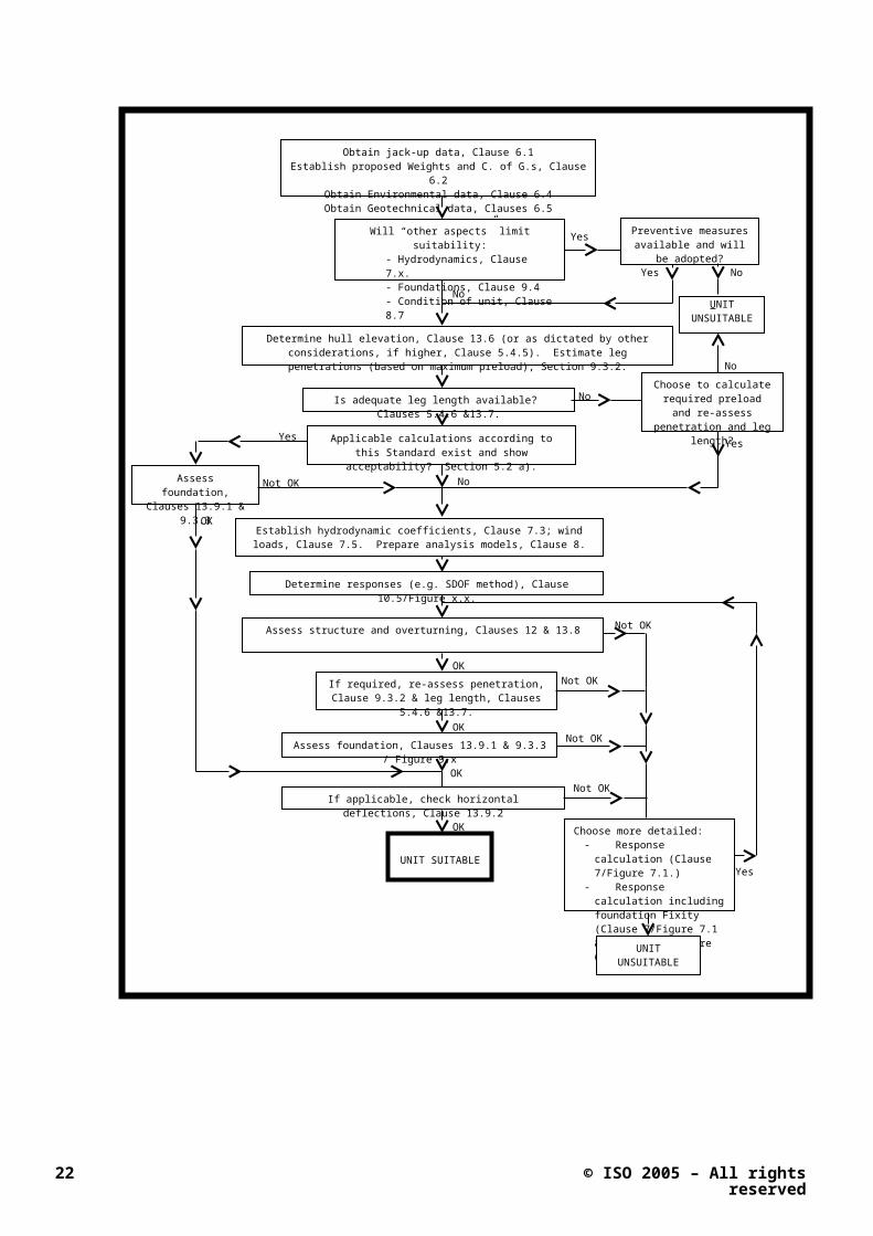
7.3.4 Wind loads
Wind loads shall be computed. using wWind velocities and wind profiles as presented in A.6.4.6 may be used. These loads may be calculated using appropriate formulae and coefficients or may be derived from applicable wind tunnel tests. Generally, for site assessments, block areas may be used for the hull, superstructures and appurtenances.
Wind loads on legs can be a dominant factor for jack-ups operating at less than their maximum design water depth.
7.4 Functional loads
For functional loads it is usual to consider the jack-up in the fully loaded condition for structural checks and with the minimum anticipated variable load (often 50%) for the overturning calculation. If the assessment of the jack-up shows it is marginal in one of these conditions, consideration may be given to limiting the variable load to a lower or higher level (depending on the critical parameter), providing the jack-up can be successfully operated under such restrictions. The assessor shall document any restrictions on the variable loads that apply to the operating limits for the site and ensure that these limits are included in the operating procedures for the site.
7.5 Displacement dependent effectsloads
Indirect loadsLoad effects that are a consequence of the displacement of the structure shall be considered in the analysis. These effects are due to the first order sway (P-delta), and theirits enhancement due to the increased flexibility of the legs in the presence of axial loads (Euler amplification).
7.6 Dynamic effects
The Indirect loads due to dynamic response of the jack-up shall be considered, and is are particularly important for seastates having significant energy near the natural periods of the jack-up or multiples thereof.
7.7 Earthquakes
Earthquake loads Loads and load effects due to earthquakes shall be considered where appropriate.
7.8 Other Loads
Other types of load may can occur in certain geographical regions, for example loads due to ice and snow loading. These loads shall be computed and applied in combination with other appropriate concurrent loads.
© ISO 2005 – All rights reserved 27

8 Structural modelling
8.1 ScopeApplicability
This clause presents the provisions for the development of an analytical model of a jack-up structure. Included in a jack-up structure are the legs, hull, leg-to-hull connection, and spudcans. The modelling of the foundation is not considered in this clause, but is presented in Clause 9.
The modelling provisions cover the generation of stiffness, self-weight, mass and application of loads.
8.2 General Overall considerations
8.2.1 General
In general, structural modelling for the assessment of a jack-up should achieve the following objectives for both the static and dynamic responses:
Realistic global response (e.g. displacement, base shear, overturning moments) for the jack-up under the applicable environmental and functional loads;
Suitable representation of the leg, leg/hull connection and the leg-foundation interaction, including non-linear effects as necessary; and
Sufficient detail to allow for assessment of the leg structure, structural/mechanical components of the jacking and/or fixation system and the foundation.
8.2.2 Modelling philosophy
The purpose of structural modelling is to estimate the forces and displacements in a structure when subjected to the calculated applied loads.
Global load distribution and estimates of forces and displacements may be obtained through use of simplified, equivalent modelling techniques.
To determine displacements and forces in the leg, leg/hull connection, leg/spudcan connection, and hull displacements, a finite element (FE) model shall be developed.
An explicit model of the conductor is rarely warranted.
8.2.3 Levels of FE modelling
In general, a jack up model shall include the leg, leg/hull connection and representative hull structure. FE models may contain combinations of detailed and simplified structural modelling. Four modelling techniques are summarised below.
a) Fully detailed model of all legs and leg/hull connections with detailed or representative stiffness model of hull and spudcan.
b) Equivalent stick leg and equivalent hull. Equivalent stiffness model of all legs and spudcans, equivalent leg/hull connection springs and representative beam-element hull grillage.
c) Combined equivalent/detailed leg and hull. Simplified lower legs and spudcans, detailed upper legs and leg/hull connections with detailed or representative stiffness model of hull.
d) Detailed single leg (or leg section) and leg/hull connection model. This model is to be used in conjunction with the reactions at the spudcan or the forces and moments in the vicinity of lower guide obtained from Model (b).
28 © ISO 2005 – All rights reserved

8.3 Modelling the leg
8.3.1 General
The leg may be modelled as a 'detailed leg', an 'equivalent leg' or a combination of the two.
8.3.2 Detailed leg
A ‘detailed leg' model consists of all structural members such as chords, horizontal, diagonal and internal braces of the leg structure and the spudcan (if required). Each structural component of the leg is represented by one or more appropriate finite elements. In the development of a detailed leg model, the use of beam elements is generally accepted practice. However, other finite elements may be utilized when necessary to accurately represent individual structural members.
8.3.3 Equivalent stick leg (stick model)
An 'equivalent leg' model consists of a series of collinear beam elements (stick model) simulating the complete leg structure. In this model, a series of one or more beam elements represent the overall stiffness characteristics of the detailed leg.
8.3.4 Combination detailed and equivalent stick leg
In this model, the areas of interest are modelled in detail and the remainder of the leg is modelled as an equivalent stickleg.
8.3.5 Stiffness adjustment
The leg stiffness used in the overall response analysis may account for a contribution from a portion of the rack tooth material. Unless detailed calculations indicate otherwise, the assumed effective area of the rack teeth should not exceed 10% of their maximum cross sectional area. When checking the capacity of the chords the chord properties should be determined discounting the rack teeth. <<< Note: a statement re. Chord properties applicable to the different inputs to acceptance checks should also be included in Clause 12 >>
8.3.6 Leg inclination (add to response section)
The additional leg moment due to leg inclination resulting from leg-hull clearances and hull inclination shall be considered (see 10.5.4), but need not be explicitly modelled.
The designed-in leg inclination of slant-leg jack-ups shall be modelled explicitly.
8.4 Modelling the hull
8.4.1 General
The hull structure shall be modelled so that the loads can be correctly transferred to the legs and the hull flexibility is represented accurately.
8.4.2 Detailed hull model
The detailed hull model shall include primary load carrying structures explicitly modelled with appropriate finite elements.
8.4.3 Equivalent hull model
If a detailed hull model is not used, an equivalent hull model shall be constructed using a grillage of beams.
© ISO 2005 – All rights reserved 29

8.5 Modelling the hull/leg/hull connection
8.5.1 General
The leg/hull connection controls the distribution of leg bending moments and shears carried between the guides and the jacking/fixation system. In the elevated condition the most heavily loaded portion of the leg is normally within the vicinity of the leg to hull connection. The stress levels in this area depend on the design concept of the jack-up. The model shall provide the means to identify any possible leg to hull contact at locations other than the guides.
8.5.2 Guide systems
The guide structures shall be modelled to restrain the chord member. When chord to guide contact occurs in the span between chord-brace connections, significant local chord bending moments may can occur. Therefore, various guide positions should be investigated.
8.5.3 Elevating systemJacking (or elevating) pinions
The jacking pinionselevating system shall be modelled based either on the pinion stiffness derived from detailed analysis or testing. Generally, the manufacturer specifies this information.
8.5.4 Fixation system
The fixation system shall be modelled to resist both vertical and horizontal forces.
8.5.5 Shock pad – floating jacking systems
For floating jacking systems, the shock pad stiffness shall be modelled and the shock pad shall be modelled to resist vertical compressive forces only. Generally, the manufacturer specifies the stiffness information.
8.5.6 Jackcase and associated bracing
The jackcase or jackhouse structures and associated bracing shall be modelled based on their actual stiffness.
8.5.7 Equivalent leg/hull stiffness
The model shall represent the overall stiffness characteristics of the leg-to-hull connection.
8.6 Modelling the spudcan and foundation
8.6.1 Spudcan structure
The spudcan structure shall be modelled sufficiently to achieve an accurate representation of the load transfer of the seabed reaction into the leg structure.
Where there is insufficient data available regarding the structural capacity of the spudcans the suitability of the spudcans for the site shall be determined from applicable analysis methods.
8.6.2 Seabed reaction point
The selected reaction point at the spudcan shall be specified clearly in the assessment. Selection of the reaction point shall be based on the estimated penetration using geotechnical information from the site and shall consider any anticipated horizontal eccentricity.
30 © ISO 2005 – All rights reserved

8.6.3 Foundation modelling
For analyses of an independent leg jack-up unit under elevated storm conditions the foundations may normally be assumed to behave as pinned supports, which are unable to sustain moment. Analysis and practical experience suggest that this may be a conservative approach for bending moment in the leg in way of the leg/hull connection.
In cases where the inclusion of rotational foundation fixity is justified and is included in the structural analysis, the nonlinear soil-structure interaction effects shall be taken into account. The model shall include the interaction of rotational, lateral and vertical soil forces. Methods of establishing foundation fixity are given in 9.
When fixity brings the structural natural period closer to the excitation frequency, the inclusion of foundation fixity may amplify the response and shall therefore be considered.
For assessing the spudcans, the leg-to-can connection and the lower parts of the leg, the foundation model shall be adequate to determine the spudcan reactions including moment.
<< Note: Panel 5 to provide guidance on foundation modelling for seismic analysis. >>
8.7 Mass modelling
The mass model shall reflect the mass distribution of the jack-up. The model shall include structural and non-structural mass, including entrapped fluids and added mass. The added mass shall be computed based on the displaced volume of the submerged members including marine growth acting in the direction of motion normal to the member. The mass associated with consumables stored within the hull (i.e. variable load) should be included in the mass model but loads such as conductor tension and hook loads should not.
The structural mass shall include:
Legs;
Hull structure; and
Spud cans.
The non-structural mass shall include:
Hull equipment and outfitting;
Variable load;
Seawater supply system;
Leg appurtenances;
Marine growth; and
Entrapped water in flooded members and spudcans.
Added mass shall include contributions from:
Submerged leg chords and braces;
Seawater caissons; and
Spud cans.
© ISO 2005 – All rights reserved 31

8.8 Application of loads and load effects
8.8.1 The assessment loadset
The assessment loadset, Fd, shall be determined using the following generalized form before application within the structural response analysis:
Fd = f,G.G + f,Q.Q + f,E[Ee + f,D.De]
where the loads are defined as: << Need to ensure that this section is compatible with clause 7. >>
G = Permanent Load: Load due to the weight of the structure and non-varying loads positioned to represent their vertical and horizontal distribution.
Q = Variable Load: Load due to maximum or minimum variable load, as appropriate, positioned at the most onerous centre of gravity location applicable to conditions under consideration. .
Ee = Environmental load: Load due to the assessment return period wind, wave and current conditions.
De = Dynamic response: Response due to the inertial loadset which represents the contribution of dynamics over and above the quasi-static response due to Ee, see 10. .
and the load factors are given by;
f,G = 1.0 and is applied to the permanent loads
f,Q = 1.0 and is applied to the variable loads
f,E = 1.15 when applied to the 50-yr return period independent extreme environmental loads
= 1.25 when applied to the 100-yr return period joint probability environmental loads
f,D = 1.0 and is applied to the dynamic response
NOTE Reference may be made to the Table in Annex B which contains all of the applicable factors to be used in a site specific analysis.
The loads and load effects to be included in the analysis are outlined as follows:
8.8.2 Permanent and variable loads
The permanent gravity loads due to hull lightweight including:
- Weight in air including appropriate solid ballast;
- Equipment or other objects;
- Buoyancy; and
- Permanent enclosed liquid.
together with the variable and functional loads shall be modelled to represent their correct vertical and horizontal distribution.
32 © ISO 2005 – All rights reserved

8.8.3 Hull sagging
Hull sagging resulting from distributed loading and hull flexibility may impose bending moments on the legs. It shall be verified that the amount of hull sag-induced moment transferred to the legs in the analytical model is appropriate given the operating procedures of the jack-up and site-specific conditions.
8.8.4 Environmental loads
The wind loading on the legs and hull shall be modelled to represent the correct vertical and horizontal distribution.
The wave/current loading on the leg and spudcan structures above the mudline should be modelled to represent their correct vertical and horizontal distribution.
8.8.5 Inertial loads
Depending on the dynamic approach adopted, (see Clause 10), inertial loads may be applied as a single point load at the hull, distributed loading on the hull or a complete set of distributed loads applied on the hull and legs.
8.8.6 Large displacement effects
P-delta effects occur because the jack-up is a relatively flexible structure and is subject to lateral displacement of the hull (sidesway) under environmental loads.
P-delta effects shall be included in the structural response.
8.8.7 Conductor loads
Although an explicit model of the conductor is rarely warranted, the factored tension and hydrodynamic loads shall be included in the analysis.
8.8.8 Earthquake loads
<< Expect input from Panel 5 - or is 10.7 all they will provide? >>
9 Foundations
<< all footings to be spudcans unless footing is essential >>
9.1 Scope
This clause addresses the geotechnical considerations, soil-structure interaction, capacity, stiffness and hazards associated with the foundations supporting independent leg jack-ups.
NOTE Mat-supported rigs are not covered and may be included in a future revision.
9.2 General
Adequate geotechnical and geophysical information shall be made available to assess the foundation stability of the jack-up at the site. Applicable information from previous operations, other surveys or activities in the area may be used in the assessment of site conditions. Soil investigation shall be carried out for areas sites where there is are no data available from previous operations. In areas where information is available, it may be possible to use such information or information obtained from other surveys or activities in the area. See 6.5 and A.6.5.for details of the recommended geotechnical and geophysical information.
The objective of the assessment is to ensure that the foundation is adequate to carry static, cyclic, and transient loads without excessive settlement or movement. The assessment shall consider:
© ISO 2005 – All rights reserved 33

The possibility of punch through;
The effects of cyclic loading;
The consequences of excessive movement of the spudcans;
The positioning of spudcans on hard sloping seabed strata; and
The effects of local soil disturbances on the stability of the footingsspudcans; such disturbances include but are not limited to footprints left by previous jack-up footings, conductor installation, scour, etc.
9.3 Geotechnical analysis of independent leg foundations
9.3.1 General
The loading imposed on the foundation during a storm due to wave in combination with wind and current is time varying and random in nature. The response to the horizontal, vertical and rotational forces on the spudcan and the embedded portion of the leg arising from the imposed loading is nonlinear and hysteretic. The nonlinearity of the foundation may have a major impact on dynamic response of the structure.
Foundation fixity is the rotational restraint offered by the soil supporting the spudcan. The degree of fixity is dependent on the soil type, the maximum vertical spudcan load during installation, the foundation stress history, the structural stiffness of the jack-up, the geometry of the footings spudcans and the combination of vertical and horizontal loading under consideration. Foundation fixity in dynamic analysis of the structure can be included in two different ways: 1) Fully Nonlinear Model and 2) Linearised Fixity Model. These methods are described in ?A.x.
The behaviour of the foundation under the action of combined loading is appropriately described by a theoretical yield surface in vertical, horizontal and moment load space. Foundation safety assessment is achieved by comparing the imposed loads with the yield surface.
9.3.2 Leg penetration during preloading
The purpose of preloading is to develop adequate foundation capacity to resist the extreme vertical and horizontal loading. The jack-up should normally have sufficient capacity to apply preload in excess of the maximum factored vertical soil loading determined for the assessment. Where there is insufficient preload capacity to meet the extreme loading, a lower preload may be acceptable when justified by appropriate geotechnical considerations (e.g. Level 3 of Clause 9.3.3).
The methods for calculating ultimate vertical bearing capacity of a foundation in various types of soil are discussed in A.9.3.2. The predicted footing spudcan penetration is obtained from the bearing capacity versus footing spudcan penetration curve at the specified preload. Uncertainties regarding the geotechnical data should be properly reflected in the interpretation and reporting of analyses.
9.3.3 Foundation stability assessment
The overall foundation stability shall be assessed. The stability may be assessed using any of the three methods below with each level increasing in order of complexity (See Figure A.9.3-8). Any higher level check need only be performed if the lower level check fails to meet the foundation acceptance criteria given in Clause 13.8:
Level 1 Preload and Sliding Check (Clause A.9.3.2.1). Loads from pinned footing spudcan analysis.
Step 1a The foundation capacity check is based on the preloading capability.
Step 1b Sliding of the windward leg is also checked (Clause A.9.3.2.2).
Level 2 Bearing Capacity Checks.
34 © ISO 2005 – All rights reserved

Step 2a Bearing capacity check (Clause A.9.3.2.2), based on resultant loading, assuming a pinned footingspudcan. Also check sliding.
Step 2b Bearing capacity check (Clause A.9.3.2.3), including rotational, vertical and translational foundation stiffness.
Level 3 Displacement Check (Clause A.9.3.2.4).
Step 3a Simple check using leg-penetration curve.
Step 3b Numerical analysis of the complete jack-up, e.g., finite Element approach
Under pinned conditions, the maximum vertical load is expected to occur on the leeward leg. Likewise, the minimum vertical load is expected on the windward leg. In Step 1, the preload check of the leeward leg is based on the assumption that the ultimate vertical bearing capacity is equal to the maximum footing spudcan load during preloading. The sliding check of the windward leg shall also be performed to ensure that the sliding capacity is adequate under minimum vertical loading conditions. (See Clause 7.2 on selection of load cases)
In Step 2a, the bearing capacity of the leeward leg shall be checked for the combined vertical and horizontal leg reactions. A reduction in vertical bearing capacity of a spudcan footing occurs when it is simultaneously subjected to horizontal and moment loading. The latter is ignored in Step 2a analyses as the spudcans footings are considered to be pinned. The sliding check of the windward leg shall be performed similarly to Step 1b.
For Step 2b, the loads are for a spudcan footing with ‘fixity’ conditions. Inclusion of foundation fixity in an assessment incorporates a check on bearing capacity in terms of vertical and horizontal (sliding) capacities. The amount of rotational fixity is not directly involved in a checking equation, but it serves to modify the forces in both the foundation and structure. The bearing and sliding checks are performed implicitly through the use of a yield function described in Annex A9.3.2.3.
When a Level 2 assessment results in an overload situation, Level 3 may be used to calculate the associated displacements. The procedure shall account for the load redistribution resulting from the overload and displacement of the spudcan(s). The displacements derived from the analysis shall be checked against the allowable displacements of the spudcans and should satisfy the following requirements:
The spudcan vertical and horizontal displacements shall not lead to unacceptable overturning or strength checks; and
The resulting rotation of the jack-up shall neither exceed the limitations defined by the operating manual nor lead to the possibility of contact with any adjacent structure.
For Step 3a, this may be accomplished by identifying the enhanced preload level that would be required to expand the V-H yield surface such that the factored capacity exceeds the applied loading. The displacement associated with this required preload is then obtained from the load-penetration curve. If the displacement is significant the effects on the foundation loads shall be evaluated and the procedure iterated.
The displacement check in Step 3b should be performed using a structural model including non-linear soil response. The displacements and rotations from a fully non-linear load-displacement foundation model shall be checked against the allowable displacements.
9.3.4 Skirted spudcans
Special considerations shall be given to the analysis of skirted spudcans including but not limited to:
Bearing capacity
Settlement including consolidation of trapped soils
Sliding resistance
© ISO 2005 – All rights reserved 35

Drainage paths
9.4 Other considerations
9.4.1 Footprint considerations
The seabed depressions, which remain when a jack-up is removed from a site, are referred to as 'footprints'. The form of the depression depends on several factors such as the spudcan shape, the soil conditions, the spudcan footing penetration achieved and the method of extraction. The shape and the time period over which the depression exists may also be affected by the local sedimentary regime.
The positioning of spudcans very close to, or partially overlapping, footprints shall be carefully considered. This is because the difference in resistance between the original soil and the disturbed soil in the footprint area and/or the slope at the footprint perimeter. The resulting leg displacements and/or eccentric spudcan loading could cause damage to the jack-up. The situation may be complicated by the proximity of a fixed structure or wellhead. <<Added post issue of N375 >> A reference is provided in Annex A.
One preventive approach is avoidance (i.e., positioning spudcans at some minimum distance away from the footprints) while a mitigative approach is leg stomping. (This may need to go to the Informative.)
9.4.2 Hard sloping strata at or below mudline
Problems associated with positioning of spudcans on a hard sloping stratum shall be carefully considered. In this respect, a hard stratum is a soil layer where only partial spudcan penetration is expected and can be either a surface or a buried feature. Where a spudcan partially penetrates into a hard sloping stratum, there is potential to generate eccentricity in the spudcan reaction.
9.4.3 Leaning instability
Leaning instability of jack-ups can occur during operations in soft clays where the rate of increase in bearing capacity with penetration is small, leading to uncontrollable leg penetration. The potential for and consequences of such instability shall be considered.
9.4.4 Leg extraction difficulties
Prior to emplacement of the jack-up unit consideration shall be given to potential leg extraction difficulties.
9.4.5 Liquefaction and cyclic mobility
Liquefaction, or cyclic mobility, occurs when the cyclic stresses within the soils cause a progressive build up of pore pressure. The excess pore pressure within the profile may build up to a stage where it becomes equal to the initial average vertical effective stress, resulting in liquefaction. Cyclic mobility may occur at a lower excess pore pressures. Foundation failure may result depending on the extent of pore pressure developed.
Such failures may be manifested as continued foundation settlements or large-scale failure of the soil mass as described above. In areas where liquefaction is known to be possible its potential shall be assessed.
For further guidance refer to Annex A.
9.4.6 Seafloor instability
Seafloor instability can be caused by a number of mechanisms, which may be interactive or act independently. The most frequent types of instability result in large-scale mass movement, in the form of mudslides or slope failures. Such phenomena are often associated with deltaic deposits, and it is recommended that expert advice be obtained when such situations are encountered.
36 © ISO 2005 – All rights reserved

Such failures may be manifested as continued foundation settlements or large-scale failure of the soil mass as described above.
For further guidance refer to Annex A.
9.4.7 Scour
When a footing spudcan is installed on the seafloor, its presence can cause increased local current velocities, which may result in the seafloor soils being eroded. The phenomenon of scour is observed around spudcans that are embedded in granular materials at sites with high seafloor current velocities, and as such the key ingredients for scour to occur are:
Hydrodynamic conditions
Flow disturbance due to presence of an obstruction
Erodibility of seafloor material
For the hydrodynamic conditions, the combination of tidal and non-tidal current velocities (e.g. storm driven currents) are found to be key parameters, so that the effects of scour can increase rapidly during storm conditions, particularly when the two contributions are aligned.
The maximum depth of scour adjacent to the spudcan is related to the dimensions of the obstruction introduced, either the spudcan itself or the spudcan in combination with the leg structure.
Particle size has a strong influence on the erodibility [McDowell & O’Connor 1977]. The larger particle sizes such as gravels and cobbles may be useful for scour protection measures if not part of the original seafloor soils.
Scour is more important for spudcans with limited seafloor penetration, as the removal the soil may result in:
A redistribution of leg load or loss of jack-up hull trim;
A reduction of the bearing capacity of the foundation and seabed fixity;
Eccentricity in the spudcan reaction;
Increase in an existing potential for punch-through.
There is no definitive procedure for the evaluation of scour potential, but useful reference material may be found in Sweeney et al (1988), Whitehouse (1998), and Rudolph et al. (2005). Previous operational experience may help in the management of scour, either in the development of scour protection measures or of an awareness of the critical combination of tidal and non-tidal (storm driven) currents that may induce scour.>>
If scour is recognised to be a potential problem, then preventive measures should be implemented. These measures may include:
a) Gravel dumping prior to installation provided the selected gravel gradation will not cause damage to the jack-up spudcans. Particularly for the larger materials, care must be taken to ensure that this activity does not adversely affect future jack-up emplacements.
b) Use of frond mats, gravel bags, gravel or grout mattresses after installation. The requirement for this may be evaluated from scour surveillance monitoring. .
c) Use of stone/gravel dumping, gravel bags or grout mattresses after installation.
d) Monitoring and adjusting for loss of airgap.
© ISO 2005 – All rights reserved 37

9.4.8 Shallow gas
Gas charged sediments might result in hazards during site investigation soil borings, reduced bearing capacity, unpredictable foundation behaviour (due to seabed depressions or gas accumulations under the spudcans) and complications with shallow drilling operations, including blowouts.
The presence of gas charged sediments may be identified by geophysical digital high-resolution shallow seismic surveys using attribute analysis techniques.
Any gas concentration should be avoided if it is located above the primary casing shoe level or the conductor pipe shoe level that are determined during the drilling program design. This is because neither of these holes are drilled under BOP control and, therefore, there is a risk of seabed cratering around the well which could result in the undermining of the footingspudcans in the event of a blow out.
Of lesser risk is the potential for gas migration from depth to the surface outside the casing. Although this occurrence is uncommon the potential should be considered.
9.4.9 Spudcan – pile-interaction
For jack-ups located in close proximity to pile-founded structures, soil displacements caused by the spudcan penetration may induce lateral loading on the nearby piles. The magnitude of the soil displacement depends on the spudcan proximity (spudcan edge-to-pile distance), the spudcan diameter, penetration, and soil stratigraphy. If the foundation materials comprise either a deep layer of homogeneous firm to stiff clay or sand and i If the proximity of the spudcan to the pile is greater than one spudcan diameter, then no significant pile loading is expected in a homogeneous single-layer soil system. On the other hand, a proximity of one spudcan diameter may not be sufficient if the soil stratigraphy consists of interbedded clay and sand layers. When the proximity is closer than one spudcan diameter or interbedded soil conditions are encountered, then analysis by the platform owner is recommended to determine the consequences of the induced pile loading.<< __________ = Added after release of N-375 >> Suggest to change the above to “if the site conditions do not consist of homogeneous soils, ……
Guidance regarding the analytical procedures available for assessing these spudcan induced pile loads is given in Annex A9.3.
38 © ISO 2005 – All rights reserved

10 Structural response
10.1 ScopeApplicability
The response of a jack-up unit is determined by applying the loading to the structural model to determine the internal forces in the members and the reactions at the foundations. The responses are to be compared with the resistances to determine the safety of the jack-up.
This section presents methods for calculating the response of a jack-up including static and dynamic effects. This section also presents a discussion of the important parameters affecting the dynamic response including mass, stiffness and damping. Stiffness and mass modelling, as well as application of loads is addressed in 8. Foundation modelling is addressed in 9 and environmental loading is presented in 7.
10.2 General considerations
Action effects required for the assessment of jack-ups typically include:
Component forces from which the adequacy of components may be checked;
Reactions from which foundation performance and global stability may be checked;
Displacements and vibrations for which the acceptability may be checked; and
When required for Long Term Operations (see 11), local stresses and cyclic behaviour from which fatigue resistance may be assessed.
10.3 Types of analyses and associated methods
A jack-up shall be assessed for in-place elevated storm environmental conditions and may need to be assessed for fatigue resistance, accidental situations, earthquake and abnormal environmental events.
Different methods of analysis may be used for the various limit states to be considered. The methods of analysis include:
Deterministic analysis in which the assessment response is determined from a single combination of actions for a given worst case analysis condition;
Stochastic analysis in which the assessment response is determined statistically as the extreme value of multiple responses.
Whether the method is primarily manual or based on analysis with computers, the analyses shall consider the parameters discussed in the following clauses. Much of the Normative text and associated Informative text is directed at computer analysis.
10.4 Generic factors
10.4.1 General
This clause presents a description of important parameters that are applicable to all methods of analyses.
10.4.2 Natural periods and affecting factors
10.4.2.1 General
The estimation of the natural period is critical in the determination of the structural response because jack-ups can exhibit a significant dynamic inertial response (above the static response). The assessment of response should
© ISO 2005 – All rights reserved 39

consider the implication of not only the accuracy of the estimate of the natural period but also the implications of variation in the natural period. Determining the correct natural period depends upon accurate estimates for the:
nature of the foundation, water depth and hull elevation; and
magnitude and location of permanent and variable loading (mass)
10.4.2.2 Stiffness
The overall stiffness of the jack-up shall include the hull, legs, leg/hull connection, foundation and the P-delta geometric effects as defined by the modelling practices in 8. A range of stiffness values should be considered where stiffness information is less well defined.
10.4.2.3 Mass
The mass model shall include contributions from structural, non-structural and added mass.
For all analysis types, the most likely mass distribution should be considered. For example, the position of the cantilever, the variable loads present, and the level of marine growth. A range of mass values or distributions should be considered where information is less well defined.
10.4.2.4 Variability in natural period
There are several factors that can cause variability in natural period. The natural period of the jack-up may change as a function of the static and possibly the time varying loading due to nonlinearities in the structural and foundation response. Structural nonlinearities may result from stiffness changes (gap impact, yielding, etc.). Foundation nonlinearities may result from changes in stiffness as a function of load level with respect to the yield surface and hysteresis.
NOTE The calculated period may vary considerably between linear elastic and nonlinear analyses.
10.4.3 Damping
System damping contributors include foundation, hydrodynamic and structural damping. Nonlinear behaviour of the foundation and jacking system also contribute to system damping. The degree to which each of these contributes to damping will depend on the type of analyses and the level of system response.
10.4.4 SoilsFoundations
Foundation response modelling is described in 9.
10.4.5 Storm ExcitationStorm excitation
Wind, current and wave all contribute to the storm excitation. The primary source of dynamic excitation is from the fluctuating nature of waves.
<< >> Panel edit inadvertently omitted from N 375
As waves and currents interact these two environmental factors should be considered in combination when generating time varying hydrodynamic drag forces according to 7 and A7.
The effects of wave directionality and spreading may be considered. When using joint probability data, all the supplied combinations of wind, wave and current shall be considered to determine maximum response. << request Panel ½ to include description of critical combinations of JP to be assessed.>>
NOTE In a deterministic calculations, waves with a periods close to the natural period of the jack-up will give the largest dynamic amplification, but this may not necessarily result in the largest response. Therefore, waves with peak periods closest to the natural period of the jack-up should be considered.
40 © ISO 2005 – All rights reserved

10.5 Storm analysis
10.5.1 General
For typical jack-up assessments, the time-varying nature of the wave loading will amplify the quasi-static responses and shall be considered. The extreme response including the quasi-static and dynamic effects can be assessed either by a quasi-static analysis procedure (A.10.5.2) including an inertial loadset (A.10.5.2.1.) or by a more detailed dynamic analysis procedure (A.10.5.3).
Gravity and wind loading shall be combined with deterministic or stochastic wave and current loads. Inertial loading is implicitly included in stochastic analysis but shall be explicitly added to the deterministic analysis. (also see A.7.2.2).
Increased leg bending moment due to leg inclination shall be combined with bending moment due to extreme response analysis prior to completing member strength checks.
10.5.2 Deterministic storm analysis
The most common method of analysis adopted for the determination of the extreme response is the deterministic, quasi-static wave analysis. This method approximates the random nature of wave excitation and implicitly assumes that the extreme response is uniquely related to the occurrence of the extreme wave. For all cases, the loads shall be calculated as given in 7. Deterministic responses are normally calculated by stepping the wave through the structure. The extreme response is determined by combining the quasi-static wave-current loading with wind loads, fixed loads, variables and an inertial loadset to represent the loading due to dynamic response.
The inertial load used in a deterministic storm analysis represents the dynamic response to the wave. Inertial loads are determined from a dynamic amplification factor (DAF). Methods of calculating the DAF include:
Direct methods such as a single degree-of-freedom approximation
Indirect methods such as estimating the ratio of quasi-static and dynamic responses
10.5.3 Stochastic storm analysis
The stochastic method for storm analysis estimates the response of the jack-up by evaluating extreme value statistics from an analysis of response to a seastate described by random variable statistics. This response may be evaluated in the time domain.
The selection of environmental load parameters is defined in 7. The environmental load parameters shall include wind and current effects. The extreme response is determined by combining the wave-current loading with wind loads, fixed loads and variables to represent the loading due to dynamic response.
10.5.4 Leg inclination
The leg moment due to leg inclination shall be combined with the leg moment due to extreme response when undertaking the structural strength checks. This will normally be accomplished by increasing the effective moment in the leg at the lower guide by an amount equal to the offset times the factored vertical reaction at the leg base. <<do we need additional language to describe methods of accounting for leg inclination??>>
10.5.5 Limit state checks
For extreme response analysis, limit state checks shall be made for the following:
Strength of leg members, particularly in the vicinity of the upper and lower guides and adjacent to leg to spud can connections;
Capacity of holding systems and jackhouse to deck connections. Hull capacities are considered to be covered by Classification unless special circumstances apply;
© ISO 2005 – All rights reserved 41

Overturning stability (related to foundation sliding); and
Spudcan strength and foundation bearing capacity.
<< >> Panel edit inadvertently omitted from N 375
Checks shall be made for a range of seastate directions that are reasonable for the location to determine the maximum component check.
See also 9, 12 and 13.
10.6 Fatigue
Although fatigue should be considered, this does not imply that a detailed assessment or analysis is required. A fatigue analysis is normally undertaken during the design phase. For jack-up operations of relatively short duration, when compared with the inspection interval, a fatigue analysis is not required, provided that structural integrity is maintained through an appropriate program of inspection. For jack-up operations of relatively long duration, see 11.
10.7 Earthquake
A one-level seismic assessment procedure shall be followed. The structure shall be assessed to the ultimate limit state (ULS) for strength and stiffness, when it is subjected to a 1000yr abnormal level earthquake (ALE). Under this ALE it should sustain little or no damage. A fuller description of the earthquake assessment methods, including the ALE may be found in ISO19901-2.
If the jack-up does not satisfy this ULS assessment, additional methods beyond those presented here may be used to demonstrate that sufficient ductility and energy dissipation capacity exists to survive this event. With these additional methods, the jack-up may sustain considerable damage, but structural failures causing loss of life and/or major environmental damage shall not be expected to occur.
Since it is not possible to ready the jack-up for an earthquake, it is important to consider all reasonable weight and operating conditions. A low weight will tend to lead to a shorter natural period, and hence greater amplification. A higher weight will result in a longer period, but greater lateral loads for the same transverse accelerations.
NOTE The greatest threat to a jack-up subject to an earthquake is likely to be from the vertical influence on the soils, or due to lateral stability. In sensitive soils in seismically active areas, caution is needed. At sites where cohesionless soil conditions dominate, seismic induced soil liquefaction needs to be considered.
10.8 Accidental situations
Accidental situations shall be addressed as required by Regulatory or Stakeholder requirements.
10.9 Alternative analysis methods
<< Draft to be developed by P3 based on 19902 12.4.6 /A12.4.6 >>
10.9.1 Ultimate strength analysis
An ultimate strength analysis is intended to identify the collapse strength of the jack-up structure and foundation under the action of abnormal environmental actions and/or to determine a reserve strength ratio. The uncertainties associated with foundation capacity are significantly greater than those associated with the ultimate strength of the structure. In performing ultimate strength analyses, it is therefore important to make this distinction and to evaluate both structural and foundation failure modes. Therefore, the following strategy is recommended:
42 © ISO 2005 – All rights reserved

a) structural or foundation failure should be identified using an analysis based on mean (or best estimates) of structural steel properties and soil properties.
b) where foundation failure occurs before structural failure, structural failure should be determined assuming a foundation capacity based on upper bound estimates of soil properties. This should provide an assessment of the steel structure strength.
Ultimate strength evaluation is used to estimate the most likely collapse strength of a structure with partial resistance factors set to 1,0. Due to the absence of partial resistance factors an ultimate strength evaluation shall be interpreted and used with care.
10.9.2 Types of analysis
Methodology for performing an ultimate strength analysis can be found in 19902. The derivation of loads and foundation properties shall be according to this document.
© ISO 2005 – All rights reserved 43

11 Long-term applications
11.1 Scope
When a jack-up is to be operated on one particular site for more than the normal Classification Special Survey period of five years, the assessment criteria shall be supplemented by the provisions of this clause and Classification Society requirements.
NOTE It is recommended that the specific requirements of the Regulator related to long-term applications be investigated.
11.2 Assessment data
In addition to the data normally required for short-term assessment, further data associated with long-term use are required. These data shall include:
the duration for which the jack-up will be on the site;
a list of modifications to the jack-up which affect the loads, fatigue endurance or structural resistance;
limitations on the ability to re-level the jack-up and maintain airgap e.g. supported conductors;
deviations from the standard operating and elevated storm configurations given in the marine operations manual;
environmental data suitable for fatigue assessment, which may account for the directionality of wind, wave and current;
expected accumulation and vertical distribution of marine growth and mitigation procedures;
geotechnical data required for the assessment of long term operations; and
other data required for fatigue assessment (see 11.3.1).
11.3 Special requirements
11.3.1 Fatigue assessment
It shall be assessed and verified that the jack jack-up has a fatigue life endurance capacity with an adequate margin of safety in relation to the planned period on site. Historical jack-up and site data shall be requested from the owner.
11.3.2 Weight control
Changes in weight during the long term operations shall be monitored to ensure compliance with the assessment assumptions. Otherwise a sufficient allowance for weight growth shall be included in the assessment.
11.3.3 Corrosion protection
Adequate corrosion protection shall be implemented to cover the entire duration on site.
11.3.4 Marine Growth
The assessment shall include the effects of the long-term accumulation of marine growth.
44 © ISO 2005 – All rights reserved

11.3.5 Foundations
The assessment shall include consideration of the potential for and effects of:
long-term foundation settlement;
seabed subsidence, e.g. due to reservoir depletion;
scour; and
seabed mobility.
11.4 Survey requirements
Surveys are required to ensure that the integrity of the jack-up is maintained during the long-term application. As a minimum the jack-up owner shall develop a plan which includes the following surveys:
1) Classification Society Special Survey prior to deployment on site; and
2) Project Specific In-service inspection program (PSIIP) surveys.
The PSIIP required for long-term operations shall be developed based on:
Classification Society requirements;
the jack-up's prior operating and inspection history; and
the assessment results for the expected operations.
Seabed survey shall be included in the PSIIP for sites where scour and/or seabed mobility are known to occur. Any changes to the PSIIP, including extension beyond the initially planned duration, shall be agreed with the Classification Society and include documentation of sufficient fatigue life.
© ISO 2005 – All rights reserved 45

12 Structural strength
12.1 Scope
12.1.1 General
This clause provides basis for the determination of the structural strength of truss type legs. Limited guidance is given for other leg types; fixation system and/or elevating system and spudcan capacity including connection to the leg. The utilisation checks shall be carried out according to the equations in 13.
???Do we want to limit spudcan loading conditions, eccentricity, boulders, etc. as used to be in Clause 13???
A suitable method of carrying out the specific calculations required by this clause can be found in A12. The factors given in A.12 are specifically tied to the calculation methods presented in the informative and should be re-calibrated if other methods are to be used.
NOTE Classification Society requirements cover the design, construction, and periodic survey of the jack-up (see 1.2). Issues, such as material properties, fabrication tolerances, welds, and construction details, are addressed by the Classification Society. Similarly, other parts of the jack-up (e.g. jack house and hull structure) are also not addressed here.
EXAMPLE If the reactions within the fixation system are within the limits set by the manufacturer, then no additional assessment is required of the hull and jack house. In addition, if the spudcan reaction is within the limits set by the manufacturer, it is not necessary to check the capacity of the leg to can connection.
12.1.2 Truss Type Legs
The requirements set out below relate to chords and braces. Weld sizes, gusset plates, the strength of joints, etc. are covered by Classification Society requirements per 1.2, and should not control the overall structural integrity. Chords and braces are covered in 12.3 to 12.6.
12.1.3 Other Leg Types
Some of the checks included in the following sub-clauses will be applicable to either tubular or box-type legs but it anticipated that other documents will need to be addressed to encompass stiffened sections. (e.g. DNV-RP-C201 "Buckling Strength of Plated Structures" and DNV-RP-C202 "Buckling Strength of Shells") << This is in 'changes accepted, but not in 'mark-up' >>
12.1.4 Fixation system and/or Elevating system
Capacity of the fixation and/or the elevating system will normally be supplied by the manufacturer. The data should represent the un-factored ultimate capacity of the system, normally given in the vertical and horizontal directions.
12.1.5 Spudcan capacity including connection to the leg
Capacity of the spudcan will normally be supplied by the manufacturer. The data should represent the un-factored ultimate capacity of the system, normally given for all of vertical and horizontal loads, and moment about the horizontal axes.
12.1.6 Overview of Assessment Procedure
The basic approach shall include the following:
Classification of cross sections (12.3);
Determination of Section Properties (12.4);
46 © ISO 2005 – All rights reserved
Node-to-node Euler amplification of member loads (if not included within the structural analysis) (12.5); and
Determination of capacity of lattice leg members (tubular members (12.6), and Non-tubular or prismatic members (12.7)), or tubular / box section legs (12.8) as appropriate.
12.2 Classification of cross-sections
12.2.1 General
The strength of a steel cross-section is affected by its potential to suffer local buckling when subject to compression due to either a bending moment or an axial force. By classifying cross-sections, the need to explicitly calculate local buckling stresses is avoided. Components and cross-sections are classified as plastic, compact, non-compact (or semi-compact) and slender. When a cross-section is composed of components of different classes, it shall be classified according to the highest (least favourable) class of its compression components.
12.2.2 Classification Definitions
The following classification shall be applied:
Class 1 Plastic: Cross-sections with plastic hinge rotation capacity. Compliance with this classification enables a plastic hinge to develop with sufficient rotation capacity to allow redistribution of moments to occur within the structure. All plastic sections are inherently compact.
Class 2 Compact: Cross-sections with plastic moment capacity. Compliance with this classification enables the full plastic moment capacity of a cross-section to be developed but local buckling may prevent development of a plastic hinge with sufficient rotation capacity to permit plastic assessment.
Class 3 Non-Compact (or Semi-Compact): Cross-sections with yield moment capacity. Compliance with this classification enables the yield stress to be realised at the extreme compression fibre but local buckling prevents the development of the plastic moment capacity.
Class 4 Slender: Cross-sections that buckle locally before yield stress can be achieved. A cross-section is classified as slender if any of the compression components of the cross-section do not comply with the limits for non-compact components.
In 12.6, strength of tubular members, the presented equations account for local buckling, whether plastic or elastic. Consequently, there is no need for tubular sections to be classified to the same extent as non-tubular sections other than to identify those tubulars for which plastic hinge rotation capacity, ie, Class 1, is possible.
12.3 Section properties
12.3.1 General
These recommendations apply to rolled and welded prismatic members which may be made up of one or more components such as can be found in a chord section of a jack-up leg.
Cross-sectional properties for prismatic (non-tubular) members shall be determined as described in this sub-clause.
Cross section properties of tubular members are included within the capacity determination and are addressed in sub-clause 12.5.
12.3.2 Plastic and compact sections
For Class 1 Plastic and Class 2 Compact sections, section properties can be determined assuming fully plastic properties.
© ISO 2005 – All rights reserved 47

Where elastic section properties are determined for Class 1 and 2 sections in place of plastic section properties, these can be based on a fully effective cross-section. When determining the elastic section modulus to be used for a cross-section comprised of components having different yield strengths, the value of the section modulus used in the calculations shall be that which coincides with the onset of first yield: this may not coincide with the minimum section modulus. << this last thought could perhaps be written more clearly, Why are we using elastic properties for Class 1 & 2? >>
12.3.3 Semi-compact sections
Section properties for Class 3 Semi-compact sections shall be based on elastic properties assuming fully effective cross-sections, i.e., Ay for cross-sectional area and Sy for elastic section modulus. When determining the section modulus to be used for a cross-section comprised of components having different yield strengths, the value of the section modulus used in the calculations shall be that which coincides with the onset of first yield: this may not coincide with the minimum section modulus. << this last thought could perhaps be written more clearly >>
12.3.4 Slender sections
Cross-section properties for Class 4 Slender sections shall be determined using elastic principles. In tension, fully effective sections shall be assumed, ie, Ay and Sy. In compression, the sectional properties shall be based on effective sections.
12.3.5 Cross section properties for assessment
The nomenclature and equations required by this sub-clause to be used in assessment of members are summarised in A.12.3.5.
12.4 Moment AmplificationMoment amplification and effective lengths
If the node-to-node member Euler amplification is explicitly included in the member actions, then there is no need to amplify the moments in the capacity equations. If the structural analysis does not explicitly include the effects of node-to-node member Euler amplification, then moment amplification shall be included.
Effective length and moment reduction factors can be determined using a rational analysis that includes joint flexibility and side-sway.
12.5 Strength of Tubular tubular Mmembers
12.5.1 General
The strength of tubular members subjected to combined axial loading and bending shall be checked. The strength of members subjected to shear and torsional shear shall also be checked.
The requirements given in this clause ignore the effects of hydrostatic pressure. The validity of this assumption shall be checked for all tubular sections.
12.6 Strength of Prismatic prismatic Mmembers
The strength of prismatic members subjected to combined axial loading and bending shall be checked. The strength of prismatic members subjected to shear and torsional shear shall also be checked.
12.7 Assessment of member joints
Tubular joints shall be assessed in accordance with ISO 19902 25.8.1.2 (Assessment of structural connections). Rational analysis shall be used for non-tubular joints. The factored loads shall be determined in accordance with 8.1.3, rather than using the factors in ISO 19902 and 19901-3.
48 © ISO 2005 – All rights reserved

NOTE The intent of the joint check is to ensure that the joint is strong enough for the applied loads. There is no requirement for the joint to be sufficiently strong to withstand the member capacity loads. There may be guidance on non-tubular joints given in other clauses of ISO 19902 and 19901-3.
© ISO 2005 – All rights reserved 49

13 Acceptance criteria
13.1 Scope
This clause defines the consequence-based criteria for checking the acceptability of a jack-up for operation at a specific site.
The load and resistance factors set out in these Acceptance Criteria have been developed in conjunction with the analysis methodology set out in the rest of this document (ISO/WD 19905-1) and are valid only with said methodology. The factors may not provide adequate reliability if used with other methodologies.
NOTE This clause presently addresses the manned-nonevacuated condition (L-L1) only and is currently based on the 50 year independent extremes as given in 6.4. Other levels will be included when they are developed.
The criteria for checking the acceptability of a jack-up are discussed in this Clause, and include consideration of the following issues:
Structural strength including legs, spudcan, and holding system;
Hull elevation;
Leg length reserve;
Overturning stability;
Foundation integrity including preload, bearing, sliding displacement and punch-through; and
Temperature.
<<< With ref to “Consequence Based in 1st para: jjs: present categorisation of L1 to include any other than manned evacuated needs to be re-considered. mjrh: Other return periods can be used based on 6.4. Would like it to be “consequence based exposure level criteria (life safety PAFA).>>>
13.1.1 ULS Structural integrity
The assessment shall ensure that the acceptance criteria are not exceeded at the ultimate limit state condition. Compliance may be demonstrated through comparison with prior calculations according to this standard.
Areas that are often critical on jack-up rigs are the legs at the lower guides, the legs between guides, the pinions and/or rack teeth, the chocks and/or chock supports (if chocks are fitted) and the leg to spudcan connection.
Where foundation fixity exists, the lower parts of the leg shall be checked assuming an upper bound fixity value. Foundation fixity shall only be included in the evaluation of the upper leg when an applicable and detailed foundation study has been made.
13.1.2 SLS & ALS Structural integrity
Serviceability limit states and accidental limit states are discussed in 5.3.
13.1.3 FLS Structural integrity
For jack-up operations of duration less than the Classification Special Survey period a fatigue analysis is not required, provided that structural integrity is maintained through an appropriate program of inspection. For long term applications, fatigue shall be considered in accordance with 11.
NOTE The special survey period is normally 5 years.
50 © ISO 2005 – All rights reserved

13.2 General formulation
The assessment shall follow a partial factor format. The partial load factors shall be applied to loads as defined in other clauses (i.e. they shall be load factors, NOT load-effect factors).
NOTE Normally both partial load and partial resistance factors are greater than unity: loads will be multiplied by partial load factors and resistances will be divided by partial resistance factors.
The utilisation of a limit state shall be expressed in the following general form:
<<<Above equation needs to be corrected for Load/Action>>>
Note: This is a generalized form of the equation, and the form appropriate for each application can differ slightly. See specific clauses for the particular form of the equation to be used. <<<Added to answer NL comment on error in formulation>>>
The factored load can be generalised as
where;
A = Assessment load
f = The specific load factor for the load being assessed
Factored loads shall be determined in accordance with 8.
Action effects are determined by following the calculation methodology set out in 10 of this standard. The Factored Resistance can be defined as:
where;
C = Representative resistance <<<Characteristic needs to be changed to Representative throughout and all lower case >>>
R = The Resistance factor for the capacity being assessed
The structural and foundation resistance factors are found in 12 and 9 respectively.
The check for capacity can be generalised as:
U 1.0
where U is the utilization defined above to one significant decimal place.
© ISO 2005 – All rights reserved 51

13.3 Leg strength
13.3.1 Partial factor approach
Details of the methodology for undertaking checks on the strength of members and elements are given in 12. In general the formulation given in 13.2 shall be used to assess the utilisation of the leg structure.
Resistance factors to be used in assessing the strength of members are given in 12.***.
NOTE Reference may be made to the Table in Informative Annex B which contains all the factors to be used in a site specific analysis, however, reference should always be made to the applicable clause in the normative to ensure that the most up to date values are used.
13.3.2 Working stress approach
<< Section to be included when completed in SNAME>>
13.4 Spudcan strength
The factored pressure on the top and bottom of the spudcan shall be checked against the unfactored ultimate capacity specified by the manufacturer. Where limited information is supplied a rational approach shall be used.
NOTE This check addresses issues such as: Spudcan overburden (maximum penetration); spudcan strength (minimum penetration/bearing area); eccentric spudcan loading / sloping seabed; and existing spudcan footprints.
13.5 Holding system strength
The factored loads in the holding system shall be checked against the unfactored ultimate capacity specified by the manufacturer. Where limited information is supplied a rational approach shall be used.
13.6 Hull elevation
Sufficient hull elevation to accommodate an abnormal crest elevation shall be provided wherever reasonably practicable. A hull elevation resulting in an air gap of 1.5 metres above the extreme wave crest is considered adequate in many areas of the world.
The extreme wave crest elevation is normally determined from the extreme water level in A.6.4.4 and the wave crest in A.6.4.2.3. For assessments where it is considered important to minimise the hull elevation and where appropriate metocean databases and reliability models exist, account may be taken of the joint probability of tide, surge and crest height in determining extreme crest elevation. Alternatively, where it is not reasonably practicable to achieve this air gap, account shall be taken of wave-in-deck actions.
NOTE The air gap is defined in ISO 19900 as the clearance between the extreme wave crest and the hull. This differs from the definition historically used by the jack-up industry.
13.7 Leg length reserve
A leg length reserve above the upper guides of at least 1.5 metres should be allowed to account for any settlement, and to provide a contingency in case the actual penetration exceeds that predicted. A larger reserve may be required due to the strength limitations of the top bay or leg/hull interface considerations.
13.8 Overturning stability
The formulation given in 13.2 shall be used to assess the overturning resistance of the jack-up. The utilization shall be calculated based on:
AEOTM = Overturning moment due to factored actions Fd
52 © ISO 2005 – All rights reserved

ROTM = The factored stabilising moment based on the representative stabilising moment COTM
The overturning moment AEOTM shall be calculated from the factored environmental actions about the most critical overturning axis. For independent leg jack-ups the overturning axes shall pass through any two or more spudcan reaction points. The reaction points are given in 8.6.2 and further described in A.8.6.2.
The representative stabilizing moment COTM shall be calculated about the same critical axis as used to calculate the overturning moment and shall account for the following parameters:
The stabilizing moments due to the permanent load (at the displaced position resulting from the factored loads).
The stabilizing moment due to the most onerous combination of minimum variable load and centre of gravity applicable to extreme conditions as specified in 7.6.
The stabilizing moments due to seabed foundation fixity. Any stabilizing moments shall be calculated in accordance with 9, taking account of degradation of the rotational moment to comply with the yield surface.
The resistance factor on the representative stabilizing moment shall be taken as:
R,OTM = Resistance Factor on hull stabilizing moment = 1.0
Large deflection effects shall be included as either an increase in overturning moment or a reduction in stabilizing moment.
Note: The reduction in stabilizing moment due to large deflection effects is implicitly included within the overturning moment when the overturning moment is calculated from the reactions obtained from a large deflection analysis. Otherwise the reduction in dead and live load stabilizing moment caused by the displacement resulting from the factored loads shall be considered either as an increase in the overturning moment or as a reduction in the stabilizing moment. <<<THIS NEEDS TO BE RE-WORKED>>>
13.9 Foundation Integrity
13.9.1 Capacity check
In general the formulation given in section 13.2 shall be used to assess the foundation. The following utilisations shall be checked:
US,vhm = foundation bearing capacity
US,hvm = foundation sliding capacity
Utilisations shall be calculated using the factored foundation resistances and foundation action effect formulations given in 9.xx.
<< PCW Note amplified by MJRH: P4 Geotech Members – We may want to make sure that the deleted subsections from draft C addressing Preload, sliding and generalised capacity checks both pinned and with fixity re-appear at Clause 9 or A.9. >>
NOTE The foundation capacity check described above encompasses the traditional sliding and preload checks.
13.9.2 Displacement check
If the factored loads on any footing exceed the factored capacity discussed above a further assessment may be performed in order to show that any additional settlements and/or the associated additional structural loads are within acceptable limits (see A.9.3.2.2).
NOTE Guidance on the allowable hull inclination may sometimes be obtained from the operations manual.
© ISO 2005 – All rights reserved 53

13.9.3 Spudcan-footprint interaction
This standard does not provide criteria for evaluating the effect of spudcans interacting with existing footprints. The assessment should consider the effect on the leg load and the necessity for mitigation.
<<<Post Sept 2005 meeting note: Patrick says that this should be deleted per US comments as well>>>
13.10 Temperature
The lowest daily average air and water temperatures should be in compliance with the limits given in the operating manual.
54 © ISO 2005 – All rights reserved

Annex A(informative)
Recommendations and Information
NOTE The clauses in this annex provide guidance on the related clause in the body of the document.
A.1 Scope
Although this standard does not address the integrity of well conductors, the following references provide guidance on their assessment: << Expect input from Rupert Hunt providing references for Conductor assessment >
A.2 Normative references
No Guidance is offered.
A.3 Terms and definitions
No Guidance is offered.
A.4 Symbols
A.4.1 Symbols for Clause A.1
A.4.2 Symbols for Clause A.2
A.4.3 Symbols for Clause A.3
A.4.4 Symbols for Clause A.4
A.4.5 Symbols for Clause A.5
A.4.6 Symbols for Clause A.6
A.4.7 Symbols for Clause A.7
A.4.8 Symbols for Clause A.8
A.4.9 Symbols for Clause A.9
A = Spudcan effective bearing area based on cross-section taken at uppermost part of bearing area in contact with soil (see Figure 6.2).
As = Spudcan laterally projected embedded area.
a = Bearing capacity squeezing factor.
© ISO 2005 – All rights reserved 55

au = Adhesion.
B = Effective spudcan diameter at uppermost part of bearing area in contact with the soil (for rectangular footing B = width).
b = Bearing capacity squeezing factor.
cu = Undrained cohesive shear strength at D + B/4 below mudline.
cu1 = Undrained cohesive shear strength at spudcan tip.
cuo = Undrained cohesive shear strength at maximum bearing area (D below mudline).
cus = Undrained cohesive shear strength at D/2 below mudline.
cu,b = Undrained cohesive shear strength - lower clay below spudcan.
cu,t = Undrained cohesive shear strength - upper clay below spudcan.
dc = Bearing capacity depth factor.
= 1 + 0.2 (D/B) (max 1.5)
dq = Bearing capacity depth factor.
= 1 + 2tan(1- sin)2 D/B for D/B 1
= 1 + 2tan(1- sin)2 arctan(D/B) for D/B > 1
d = Bearing capacity depth factor = 1.
D = Distance from mudline to spudcan maximum bearing area.
f1 = Factor used in yield surface equation for embedded footings on clay.
f2 = Factor used in yield surface equation for embedded footings on clay.
fr = Reduction factor on stiffness.
Fo' = Effective overburden pressure due to back-flow at depth of uppermost part of bearing area.
FH = Horizontal foundation capacity.
FHM = Horizontal foundation capacity in combination with moment.
FV = Vertical foundation capacity.
FV,b = Ultimate vertical bearing capacity assuming the footing bears on the surface of the lower (bottom) clay layer with no back-flow.
FVH = Vertical foundation capacity in combination with horizontal load.
FVHM = Vertical foundation capacity in combination with horizontal and moment load.
FM = Moment capacity of foundation.
Gv = Shear Modulus for vertical loading.
56 © ISO 2005 – All rights reserved

Gh = Shear Modulus for horizontal loading.
Gr = Shear Modulus for rotational loading.
h = Distance from rotation point to reaction point.
h1 = Embedment depth to the uppermost part of the spudcan, (if not fully embedded = 0).
h2 = Spudcan tip embedment depth.
H = Distance from spudcan maximum bearing area to weak strata below.
HLo = (C1/C2)(VLo/4), C1 = 0.3, C2 = 0.625 (sand)
= Acuo +(cuo + cu1)As (clay)
ic = Inclination factor (for = 0).
= 1 - mFH/AcuNc
iq = Inclination factor.
= (1 - FH/FVH)m
i = Inclination factor.
= (1 - FH/FVH)m+1
I = Height of soil column above spudcan.
ka = Active earth pressure coefficient (for cu = 0) = tan2(45-/2)
kp = Passive earth pressure coefficient = 1/ka
K1,K2,K3 = Stiffness factors.
Ks = Coefficient of punching shear.
L = Foundation length, for circular foundation L=B.
m For strip footing - inclination in direction of shorter side.
= (2 + B/L)/(1 + B/L)
m = For strip footing - inclination in direction of longer side.
= (2 + L/B)/(1 + L/B)
m For circular footing = 1.5
MLo = C1VLoB/4, C1 = 0.3 (sand)
= 0.1VLoB (clay)
MP = moment capacity associated with further spudcan penetration under environmental loading (equal to minimum of MPS and MPV).
MPS = moment capacity when further spudcan penetration leads to fully seated spud conditions.
© ISO 2005 – All rights reserved 57

MPV = moment capacity under further spudcan penetration, when the actual vertical force is too low to reach fully seated conditions.
n = Iteration factor, 2.
N = Stability factor.
NC = Bearing capacity factor (taken as Nc sc= 6.0 for circular footings).
Nq = Bearing capacity factor = etantan2(45 + /2)
NY = Bearing capacity factor = 2(Nq + 1)tan
po' = Effective overburden pressure at depth, D, of maximum bearing area.
QH = Applied factored horizontal load.
QM = Applied factored moment load.
QV = Applied factored vertical load.
rf = Failure ratio.
sc = Bearing capacity shape factor = (1 + (Nq/Nc)(B/L))
sq = Bearing capacity shape factor = 1 + (B/L)tan
sY = Bearing capacity shape factor = 1 - 0.4(B/L)
( = 0.6 for circular footing under pure vertical load).
T = Thickness of weak clay layer underneath spudcan.
V = Volume of soil displaced by spudcan.
VLo = Maximum vertical foundation load during preloading.
= Adhesion factor = 1.0 for soft clays, = 0.5 for stiff clays.
= Steel/soil friction angle - degrees, (-5).
v = Vertical displacement of foundation.
h = Horizontal displacement of foundation.
Y' = Submerged unit weight of soil.
= Foundation rotation - radians.
= Angle of internal friction for sand - degrees.
v = Poisson's ratio.
58 © ISO 2005 – All rights reserved

A.4.10 Symbols for Clause A.10
A.4.11 Symbols for Clause A.11
A.4.12 Symbols for Clause A.12
A.4.13 Symbols for Clause A.13
© ISO 2005 – All rights reserved 59

A.5 Overall considerations
A.5.1 General
A.5.1.1 Planning
No Guidance is offered.
A.5.1.2 Assessment situations and criteria
No Guidance is offered.
A.5.1.3 Regulations
No Guidance is offered.
A.5.2 Assessment approach
No Guidance is offered.
A.5.3 Selection of limit states
No Guidance is offered.
A.5.4 Determination of assessment situations
No Guidance is offered.
A.5.4.1 General
No Guidance is offered.
A.5.4.2 Reaction point and foundation fixity
No Guidance is offered.
A.5.4.3 Storm approach angle
No Guidance is offered.
A.5.4.4 Weights and centre of gravity
No Guidance is offered.
A.5.4.5 Hull elevation and air gap
No Guidance is offered.
A.5.4.6 Leg length reserve
No Guidance is offered.
60 © ISO 2005 – All rights reserved

A.5.4.7 Adjacent structures
No Guidance is offered.
A.5.4.8 Other
No Guidance is offered.
A.5.5 Determination of eExposure levels
A.5.5.1 General
No Guidance is offered.
A.5.5.2 Life-safety categories
No Guidance is offered.
A.5.5.3 Consequence categories
No Guidance is offered.
A.5.5.4 Determination of exposure level
No Guidance is offered.
A.5.6 Regulations
© ISO 2005 – All rights reserved 61

A.6 Data to be assembled for each site location
A.6.1 Scope
No Guidance is offered.
A.6.2 Rig data
No Guidance is offered.
A.6.3 Site data
No Guidance is offered.
A.6.4 Metocean data
A.6.4.1 General
Experience of site assessment for manned jack-ups supports the use of the 50 year return period independent extremes. The use of 100-year joint probability environmental metocean data may be used as an alternative to the 50-year extremes. The action factors for these two alternatives differ.
In some cases a smaller return period extremes may be justified. For example, in the absence of regional guidance, if the jack-up is manned-evacuated or unmanned and the risk of environmental pollution is considered to be sufficiently low, the use of a 10-year return period storm is recommended. In such cases the availability and effectiveness of early warning systems and the adequacy of the evacuation plans should be assessed. For the manned condition prior to evacuation the historical metocean database should be reviewed for instances of sudden tropical revolving storms that could affect the location within the period of time required to evacuate the jack-up.
Safety Partial factors for each of these options are presented in ?5 and/or 13 << and/or Annex B >>.
Site specific data, if available, should be used for the assessment as regional data may not take account of local variations.
Where there is sufficient evidence that any of the environmental loads at the site are directional, it may be possible to align the jack-up on the most advantageous heading.
<<Panel 10 is to provide the factors for each of the three conditions discussed in this section. Panel 10 can consider safety factors for WSD at the same time.>>
A.6.4.2 Waves
A.6.4.2.1 Extreme wave height environment
The extreme wave height environment used for elevated storm conditions shall, as a minimum, be computed according to the following sub-sections clauses based on the three-hour storm duration with an intensity defined by the significant wave height, Hsrp, for the assessment return period. The seasonally adjusted wave height may be used as appropriate for the operation.
The wave height information for a specific site may also be expressed in terms of Hmax, the individual extreme wave height for the return period, rather than the significant wave height Hsrp. The relationship between Hsrp and Hmax
must be determined accounting for the effects of storms (longer than 3 hours) and for the additional probability of other return period storms <<see Commentary Section C3.5.1>>. This relationship will depend on the site specific conditions, however Hsrp may usually be determined from Hmax using the generally accepted relationship for non-cyclonic areas:
62 © ISO 2005 – All rights reserved

Hsrp = Hmax/1.86
For cyclonic areas the recommended relationship is:
Hsrp = Hmax/1.75
Note: The wave load can be computed either stochastically (through a random frequency or time domain approach) or deterministically (through an individual maximum wave approach). The scaled wave heights for the two approaches are discussed in A.6.4.2.5 and A.6.4.2.2, respectively <<(see Commentary)>>.. The scaled wave heights are to be used only in conjunction with the associated kinematics modelling recommended in A.7 and the hydrodynamic coefficients given in A.7.3.
A.6.4.2.2 Deterministic waves
For deterministic/regular wave load calculations it is appropriate to apply a kinematics reduction factor of 0.86 in order to obtain realistic load estimates for a 50 year storm <<(see Commentary)>>. This factor accounts for the need to ensure that both the deterministic/regular wave load calculation and 3 hour simulation produce statistically comparable results (i.e. both target the most probable maximum response in the 50 year storm). In addition, the 0.86 factor may be considered to take some account of wave spreading and the conservatism of deterministic/regular wave kinematics (traditionally accomplished by adjusting the hydrodynamic properties).
The factor should be applied by means of a reduced wave height, Hdet. Hdet may be determined as a function of Hmax from:
Hdet = 0.86 Hmax
The use of a factor smaller than 0.86 may be justified on the basis of an analysis which explicitly accounting for the effects of three-dimensional spreading. However, such effects should be properly balanced by the inclusion of second-order interaction effects between spectral wave components. <<Commentary reference to IADC/ND study on wave directional spreading?>>
The wave loads should be determined using an appropriate wave kinematics model in accordance with A.7.4.3.
In the analysis a single value for the wave period Tass, in seconds, associated with the maximum wave may be considered. The “intrinsic” period of the wave as seen by an observer moving with the current should be used in the derivation of wave kinematics required for load calculations; guidance is given in ISO 19901-1, Metocean Design and Operation Conditions, Clauses 5.2 and 8.3. Unless site specific information indicates otherwise T ass will normally be between the following limits:
3.44 < Tass < 4.42
where Hsrp is the return period extreme significant wave height in meters.
A.6.4.2.3 Wave crest elevation
For calculation to determine minimum hull elevation the wave crest elevation above the extreme still water level in A.6.4.4 may be obtained from the relationship between Hmax/Hsrp in A.6.4.2.1 above and the appropriate deterministic wave theory in A.7.4.3.
A reasonably foreseeable extreme return period should be used for this calculation, and is recommended to be no shorter than 50 years, even if a lower return period is used for other purposes. . <<Need to provide some text on how to calculate abnormal/extreme wave crest for use in 13.6, ref. SNAME NS annex / or 19901-1 >>
© ISO 2005 – All rights reserved 63

A.6.4.2.4 Wave spectrum
<< Note to 6.2.4.6 is not in a logical location - put here and move much/all of the spectral information to TR ??? ALSO: Check whether we can rely on 19901-1 for any the spectral definitions >> Where the analysis method requires the use of spectral data, the choice of the analytical wave spectrum and associated spectral parameters should reflect the width and shape of spectra for the site and significant wave height under consideration. In cases where fetch and duration of extreme winds are sufficiently long a fully developed sea will result (this is rarely realised except, for example, in areas subject to monsoons). Such conditions may be represented by a Pierson-Moskowitz spectrum. Where fetch or duration of extreme winds is limited, or in shallow water depths, a JONSWAP spectrum may normally be applied (see Note at the end of this Clause).
The wave spectrum can be represented by the power density of wave surface elevation S(f) as a function of wave frequency by:
S(f) = (16I0())-1Hs2TP(TPf)-5exp(-1.25/(TPf)4)q
[Note: An alternative formulation is given in <<the Commentary>>]
where;
q = exp(-(Tpf-1)2/22) with:
= 0.07 for Tpf <= 1
= 0.09 for Tpf > 1 (Carter 1982, [1]) <<Ensure this reference & ref. number is included in Bibliograph>>
and;
Hs = significant wave height (meters), including depth correction, according to Clause A.6.4.2.5
Tp = peak period (seconds)
f = frequency (Hz)
= peak enhancement factor
I0() = is discussed below.
The above definition yields a single parameter Pierson-Moskowitz spectrum when = 1 and Tp = 5 , with Hs
in meters. In this case an appropriate Tp/Tz ratio is 1.406 (see below).
When considering a JONSWAP spectrum, the peak enhancement factor varies between 1 and 7 with a most probable average value of 3.3. There is no firm relationship between , Hs and Tp. Relationships between variables for different according to Carter (1982) [1] <<Ensure this reference & ref. number is included in Bibliograph>>are as follows:
1233.34567
I0()
0.2000.2490.2930.3050.3340.3720.4100.446
Tp/Tz
1.4061.3391.2951.2861.2601.2411.2211.205
Alternatively:
64 © ISO 2005 – All rights reserved

Unless site specific information indicates otherwise = 3.3 may be used.
A.6.4.2.5 Effective significant wave height
For stochastic/random wave load calculations Airy wave theory is implied, see A.7.4.3. To account for wave asymmetry, which is not included in Airy wave theory, a scaling of the significant wave height should be applied to capture the largest wave loads at the maximum crest amplitude. The effective significant wave height, Hs, may be determined as a function of the water depth, d in meters, from:
Hs = [1 + 0.5e(-d/25)] Hsrp (d 25m)
and should be used with the wave kinematics model described in A.7.4.3.
For water depths less than 25m an appropriate regular wave analysis should be considered.
A.6.4.2.6 Zero-upcrossing period
For a given significant wave height the wave period depends on the significant wave steepness which in extreme seas in deep water often lies within the range 1/20 to 1/16. This leads to an expression for zero-upcrossing period Tz, related to Hsrp in meters, as follows:
3.2 < Tz < 3.6
However in shallow water the wave steepness can increase to 1/12 or more, leading to a zero-upcrossing period T z
as low as 2.8 . This is because the wave height increases and wave length decreases for a given Tz.
Note: << This is not in a logical location - put at start of 6.4.2.4 and move much/all of the spectral information to TR ??? >>
If a JONSWAP spectrum is applied the response analysis should consider a range of periods associated with H srp
based on the most probable value of Tp plus or minus one standard deviation. However it should be ensured that the assumptions made in deriving the spectral period parameters are consistent with the values used in the analysis. Alternatively, applicable combinations of wave height and period may be obtained from a scatter diagram determined from site specific measurements; in this case specialist advice should be obtained on a suitable spectral form for the site. To avoid the need for analyses of several wave periods a practical alternative is to use a 2 parameter spectrum with = 1.0 in combination with the site specific most probable peak period.
A.6.4.2.7 Short-crested stochastic waves
For stochastic/random wave load calculations, the short-crestedness of waves (i.e. the angular distribution of wave energy about the dominant direction) may be accounted for when site-specific information indicates that such effects are applicable. In all cases the potential for increased response due to short-crested waves should be investigated. The effect may be included by means of a directionality function F(), as follows:
S(f, ) = S(f).F()
where;
= angle between direction of elementary wave trains and dominant direction of the short-crested waves.
S(f, ) = directional short-crested power density spectrum.
F() = directionality function.
and, in the absence of more reliable data:
© ISO 2005 – All rights reserved 65

F() = C.Cos2n for -
where;
n = power constant
C = constant chosen such that:
/2
F() .d = 1.0-/2
<< Review Panel Jan 06: Can this text be harmonised with or reference 19901-1 ?? >>
The minimum value for the power constant n, should not normally be taken as less than:
n = 2.0 for fatigue analysis
n = 4.0 for extreme analysis
Note:
The modelling of short-crested stochastic waves in the present clause is not to be mixed-up or combined with the wave kinematics factor used in deterministic wave analysis to represent wave spreading and the conservatism of deterministic/regular wave kinematics, see A.6.2.2.
A.6.4.2.8 Non-linear wave effects
Where the natural period of the jack-up is such that it may respond dynamically to waves, see A.10.4.1, the maximum dynamic response may be caused by wave heights or seastates with periods outside the ranges given in A.6.4.2.2 and A.6.4.2.6. Such conditions should also be investigated to ensure that the maximum (dynamic plus quasi-static) response is determined.
A.6.4.2.9 Long term data
For fatigue calculations, (see 11.3.1) the long term wave climate may be required. For the purposes of the fatigue analysis the long-term data may be presented deterministically in terms of the annual number of waves predicted to fall into each height/period/direction group. Alternatively the probability of occurrence for each seastate (characterized by wave energy spectra and the associated physical parameters) may be presented in the form of a significant wave height versus zero-upcrossing period scatter diagram or as a table of representative seastates.
A.6.4.3 Current
The extreme wind driven surface current velocity should be that associated with the assessment return period wind, seasonally adjusted if appropriate. When directional information regarding other current velocity components is available the maximum surface flow of the mean spring tidal current and the assessment return period surge current, seasonally adjusted if appropriate, should be vectorially added in the down-wind direction and combined with the wind driven surface current as indicated below. If directional data are not available the components should be assumed to be omni-directional and should be summed algebraically.
Note: A site specific study will normally be required to define the current velocity components.
The current profile may be expressed as a series of velocities at certain stations from seabed to water surface. Unless site specific data indicates otherwise, and in the absence of other residual currents (such as circulation, eddy currents, slope currents, internal waves, inertial currents, etc.), an appropriate method for computing current profile (see Figure A.6.4-1) is:
66 © ISO 2005 – All rights reserved

VC = Vt + Vs + (Vw - Vs) [(h+z)/h], for z h and Vs < Vw
VC = Vt + Vs for z > h or Vs Vw
where;
VC = current velocity as a function of z. Note that a reduction may be applicable according to A.7.4.4.
Vt = downwind component of mean spring tidal current.
Vs = downwind component of associated surge current (excluding wind driven component).
Vw = wind generated surface current. In the absence of other data this may conservatively be taken as 2.6% of the 1 minute sustained wind velocity at 10m.
h = reference depth for wind driven current. In the absence of other data h should be taken as 10 meters.
z = distance above still water level (SWL) under consideration (always negative).
<< Review Panel comment Jan 06: Is the above still considered to be correct? This profile was popular for a very short period of time. What does 19901-1 recommend ? >>
Figure A.6.4-1 — Suggested current profile
In the presence of waves the current profile should be stretched/compressed such that the surface component remains constant. This may be achieved by substituting the elevation as described in A.7.4.3.2. Alternative methods may be suitable, however mass continuity methods are not recommended. The current profile may be changed by wave breaking. In such cases the wind induced current could be more uniform with depth.
For a fatigue analysis, current may normally be neglected.
A.6.4.4 Water depths
The water depth at the site should be determined and related to lowest astronomical tide (LAT). The relationship between LAT and Chart Datum is discussed in << Part 2 Commentary >>.
The mean water level (MWL) related to the seabed should be expressed as the mean level between highest astronomical tide (HAT) and lowest astronomical tide (LAT) i.e.:
© ISO 2005 – All rights reserved 67

MWL = (HAT + LAT)/2
The extreme still water level (SWL) should be expressed as a height above LAT, and should be the sum of;
Mean high water spring tide (MHWS)+ relevant return period extreme storm surge (Use a reasonably foreseeable extreme return period (not less than 50-year value) for minimum hull elevation determination).
unless reliable data indicates that an alternative summation is appropriate.
When lower water levels are more onerous the minimum still water level (SWL) to be considered in the loading calculations should be the sum of:
Mean Low Water Spring Tide (MLWS)+ relevant return period negative storm surge.
A.6.4.5 Marine growth
<< Moved to A.7.3.5 by review panel Jan 06 >>Where existing marine growth is not to be cleaned between sites or where the operation is to last long enough for significant growth to occur, the influence of growth on the leg hydrodynamic properties should be considered. Where applicable, site specific data should be obtained. In the absence of such data, default values for thickness and distribution are given in A.7.3.5.
A.6.4.6 Wind
A.6.4.6.1 General
The wind velocity used for the 50-year or 10-year storm should be the 1 minute sustained wind for the assessment return period, related to a reference level of 10.0m above mean sea level. In case the 100 year joint probability load level approach is applied the methodology presented in <<Commentary C3.A to the SNAME North Sea Annex >> may be used to determine the 100 year joint probability load level wind velocity. This wind speed may be conservatively taken as the 100 year return period individual extreme 1 hour mean wind << Review Panel query Jan 06 : IS THIS STILL ACCEPTED ?? >>. However, when wind loads dominate, the 100 year return period individual extreme 1 minute mean wind should be used. A reference level of 10.0m above mean sea level should be applied.
The wind velocity profile may be taken as a power law unless site specific data indicates otherwise.
Different jack-up configurations (weight, centre of gravity, cantilever position, etc.) may be specified for operating and elevated storm modes. In such cases, the maximum wind velocity considered for the operating mode should not exceed that permitted for the change to the elevated storm mode.
A.6.4.6.2 Wind profile
The expression for the vertical profile of the mean wind velocity in the form of a power law is:
VZ = Vref (Z/Zref)1/N
where;
VZ = the wind velocity at elevation Z above mean water level.
Vref = the 1 minute sustained wind velocity at elevation Zref (normally 10m above MWL).
N = 10 unless site specific data indicate that an alternative value of N is appropriate.
68 © ISO 2005 – All rights reserved

A.6.5 Geotechnical data
<< Info from A.9 moved to here by Review Panel Jan 06 >>
A.6.5.1 Integrated geoscience studies
Adequate geotechnical and geophysical information shall be available to assess the site and the foundation stability. Aspects, which should be investigated, are shown in Table A.6.5-1 and are discussed in more detail in the referenced sections. The information obtained from the surveys and investigations set out in Clauses A.6.5.1.1 to A.6.5.1.5 is required for areas where there is no data available from previous operations. In areas where information is available, it may be possible to reduce the requirements set out below by use of information obtained from other surveys or activities in the area.
A.6.5.1.1 Bathymetric survey
An appropriate bathymetric survey should be supplied for an area approximately 1 kilometer square centered on the proposed position at the site. Line spacing of the survey should typically be not greater than 100 meters x 250 meters over the survey area. Interlining is to be performed within an area 200 meters x 200 meters centered on the proposed position at the site. Interlining should have spacing less than 25 meters x 50 meters.
A.6.5.1.2 Seabed surface survey
The seabed surface shall be surveyed using sidescan sonar or high-resolution multibeam echosounder techniques and shall be of sufficient quality to identify obstructions and seabed features and should cover the immediate area (normally a 1 km square) of the intended site. The slant range selection shall give a minimum of 100% overlap between adjacent lines. A magnetometer survey may also be required if there are buried pipelines, cables and other metallic debris located on or slightly below the sea floor.
Where seabed obstructions such as pipelines and wellheads are known to be present, sufficient information to enable safe positioning of the jack-up is required. In some cases an ROV or diver’s inspection may be required in addition to the seabed surface survey.
Seabed surface surveys can become out-of-date, particularly in areas of construction/drilling activity or areas with mobile sediments. . At open water sites the maximum period for the validity of seabed surveys for debris and mobile sediment conditions should be determined taking account of local conditions. For positions at the sites (pending Review Panel decision) close to existing installations seabed surveys for debris and sediment conditions should, subject to practical considerations, be undertaken immediately prior to the arrival of the jack-up at the site.
A.6.5.1.3 Shallow seismic survey
The principal objectives of the shallow seismic survey are:
To determine near surface soil stratigraphy. This requires correlation of the seismic data with (existing) soil boring data in the vicinity.
To reveal the presence of shallow gas concentrations.
Due to the qualitative nature of seismic surveys it is not possible to conduct analytical foundation appraisals based on seismic data alone. This requires correlation of the seismic data with soil boring data in the vicinity through similar stratigraphy.
A shallow seismic survey should be performed over an approximately 1 kilometre square area centred on the proposed position at the site. Line spacing of the survey should typically be not greater than 100 meters x 250 meters over the survey area. Equipment should normally be capable of giving detailed data to a depth equal to the greater of 30 meters or the anticipated spudcan penetration plus 1.5 times the spudcan diameter.
© ISO 2005 – All rights reserved 69

The survey report should include at least two vertical cross-sections passing through the proposed position at the site showing all the relevant reflectors and allied geological information. The equipment used should be capable of identifying reflectors of 0.5m and thicker.
A.6.5.1.4 Geotechnical investigation
A.6.5.1.4.1 Introduction
Site-specific geotechnical investigation and testing are recommended in areas where any of the following apply:
the shallow seismic survey cannot be interpreted with any certainty
no geotechnical data is available in nearby area
significant layering of the strata is indicated
the site is known to be potentially hazardous.
A.6.5.1.4.2 Soil investigation and testing
A geotechnical investigation should comprise a minimum of one borehole to a depth equal to 30 metres or the anticipated spudcan penetration plus 1.5 times the spudcan diameter, whichever is the greater. All the layers should be adequately investigated and the transition zones cored at a sufficient sampling rate.
The number of boreholes required should account for the lateral variability of the soil conditions, regional experience and the geophysical investigation. When a single borehole is made, the preferred location is at the center of the leg pattern at the intended position at the site.
“Undisturbed” soil sampling and laboratory testing and/or in-situ piezocone penetrometer testing should be conducted. Other recognized types of in-situ soil testing may be appropriate such as vane shear and/or pressure meter tests.
A.6.5.1.4.3 Geotechnical report
The geotechnical report should include borehole logs, piezocone penetrometer records (if appropriate) and documentation of all laboratory tests, together with interpreted soil design parameters. A competent geotechnical engineer should select design parameters. For the methods recommended in Section 9.3 and 9.4, the design parameters should include profiles of undrained shear strength and/or effective stress parameters, soil indices (plasticity, liquidity, grain size, etc.), relative density, unit weight and, the over consolidation ratio (OCR).
Additional soil testing to provide shear moduli and cyclic/dynamic behaviour may be required if more comprehensive analyses are to be applied or where the soil strength may deteriorate under cyclic loading.
A.6.5.1.5 Integrated studies
The results of bathymetric surveys, seabed surface surveys, shallow seismic surveys, seabed samples and geotechnical investigations should be integrated to assess the soil conditions at the proposed site. Lateral variations of geotechnical parameters can be assessed from the correlation of the shallow seismic data and the geotechnical information from the borehole logs or piezocone penetration tests.
Table A.6.5-1 — Foundation risks, methods for evaluation and prevention
RISK METHODS FOR EVALUATION & PREVENTION
CLAUSE
Installation Problems Bathymetric survey
Seabed surface survey
A.6.5.1.1
A.6.5.2.2
70 © ISO 2005 – All rights reserved

Punch-through Shallow seismic survey
Soil sampling and other geotechnical testing and analysis
A.6.5.1.3
A.6.5.1.4,A.9.3.2.7
Settlement under storm loading/Bearing failure
Shallow seismic survey
Soil sampling and other geotechnical testing and analysis
Ensure adequate jack-up preload capability
A.6.5.1.3
A.6.5.1.4A.9.3.2.7
A.9.3.3
Sliding failure Shallow seismic survey
Soil sampling and other geotechnical testing and analysis
Increase vertical spudcan reaction
Modify the spudcans
A.6.5.1.3
A.6.5.1.4A.9.3.3.2
Scour Bathymetric and seabed surface survey (identify sand waves)
Surface soil samples and seabed currents
Inspect spudcan foundation regularly
Install scour protection (gravel bag/artificial seaweed) when anticipated
A.6.5.1.1
A.6.5.1.2
9.4.7
Geohazards (mudslides, mud volcanos etc)
Seabed surface survey
Shallow seismic survey
Soil sampling and other geotechnical testing and analysis
A.6.5.1.2
A.6.5.1.3
A.6.5.1.4
Gas pockets/Shallow gas Shallow seismic survey A.6.5.1.3
Faults Shallow seismic survey A.6.5.1.3
Metal or other object, sunken wreck, anchors, pipelines etc.
Magnetometer and seabed surface survey A.6.5.1.2
Local holes (depressions) in seabed, reefs, pinnacle rocks, non-metallic structures or wooden wreck
Seabed surface survey
Diver/ROV inspection
A.6.5.1.2
Legs stuck in mud Soil sampling and other geotechnical testing and analysis
Consider change in spudcans
Jetting/Airlifting
A.6.5.1.3
A.6.5.1.4
A.6.5.1.5
Eccentric spudcan reactions Bathymetric and seabed surface surveys
Shallow seismic survey (buried channels or footprints)
Soil sampling and other geotechnical testing and analysis
Seabed modification
A.6.5.1.1, A.6.5.1.2
A.6.5.1.3
A.6.5.1.4A.9.3 ????
Seabed slope Bathymetric and Seabed surface surveys
Seabed modification
A.6.5.1.1, A.6.5.1.2
© ISO 2005 – All rights reserved 71

Footprints of previous jack-ups Evaluate site records
Prescribed installation procedures
Consider filling/modification of holes as necessary
A.6.5.1.1A.6.5.1.2
9.4.1
9.4.1
A.7 Loads
A.7.1 Scope
This section clause presents applicable formulations and methods to calculate loads for site assessment according to the present standard.
The wave and current loads are presented for quasi-static and dynamic analysis. Normally a quasi-static, deterministic extreme wave analysis where dynamics is represented by an inertia load set, is performed for jack-up site assessment. Calculations of loads for stochastic analysis in frequency or time domain are also presented. Such analysis analyses are applicable for calculation of inertia load sets or for the direct calculations of the structural dynamic responses. The hydrodynamic formulations and coefficients are presented together with formulas for detailed and equivalent modelling of leg hydrodynamic loads.
Wind models, flow coefficients for different structural parts and load formulation for calculation of static wind loads are presented.
Principles for assessment of functional loads and response effects are presented. << Guidance/references on wave in deck loads should be provided by Panel 1-2, ref. 13.6 - perhaps reference MSL CU paper and/or 19902 >>
A.7.2 General
No guidance offered.
A.7.3 Environmental loads
A.7.3.1 General
A.7.3.1.1 Environmental load modelsLoad combinations
For the 50-year return period individual extreme environmental load model the combination of environmental load components should be:
Loading on legs and other structures subject to wave loading due to 50-year return period individual extreme wave and current,
plus
loading on hull and exposed areas (e.g., legs) as applicable due to the 50-year return period 1 minute individual extreme mean wind.
Alternatively, for the 100-year return period, joint probability load model the combination of environmental load components should be:
a) Loading on legs and other structures subject to wave loading due to 100-year return period load level wave and associated joint probability current (typically the wave height may be taken as the 100-year return period individual extreme),
72 © ISO 2005 – All rights reserved

plus
loading on hull and exposed areas (e.g., legs) as applicable due to the 100-year return period load level wind associated with the selected wave height and current velocity (typically this wind speed may be taken conservatively as the 1 hour mean 100-year return period individual extreme wind),
ORor, where the wind load exceeds the wave/current plus dynamic loads,
b) Loading on hull and exposed areas (e.g., legs) as applicable due to the 100-year return period 1 minute mean individual extreme wind,
plus
loading on legs and other structures subject to wave loading due to the joint probability 100-year load level wave and current combination associated with the selected wind velocity.
<< Guidance for unmanned operations on hold waiting for outcome of the “GoM” annex>>
A.7.3.1.2 Analysis mMethods for the determination of actions
The actions can be determined by one of two alternative methods, deterministic and stochastic. The dynamic actions for the deterministic method may be determined stochastically. In a stochastic analysis the dynamics of the jack-up and non-linearities of the loading and foundation interaction may be considered. Normally Often a deterministic quasi-static analysis should beis applied used for jack-up site assessment. In such analysis tThe environmental load calculation procedure should follow the steps in the applicable tables these steps:.
<< Review Panel suggestion Jan 06 : The lists below are very useful. They should be tabulated (see suggested layout below) and perhaps placed in the Normative. The order should be carefully reviewed to ensure the data is presented in a logical order. May need some added information (including functional, other, seismic) to link to other clauses, particularly 10. >>
Table A.7.3-1 — Deterministic approach
TOPIC Etc …
<< single word item >>
Sub-topic << as per a) - z) lists >> Reference clause(s)
Wave Height, range of associated wave periods, storm water depth, and current profile,
A.6.4.2.1 A.6.4.2.2, A.6.4.4, and A.6.4.3
A reduction factor should be applied to the wave height to determine Hdet A.6.4.2.2
Wave Theory The two dimensional wave kinematics are determined from an appropriate wave theory for the specified wave height, storm water depth, and intrinsic wave period,
A.7.3.3.3
Current The effective local current profile may be determined by multiplying the specified current profile by a factor accounting for interference from the structure on the flow field,
A.7.3.3.7
Stretching
Hydrodynamic Modelling
Model
Coefficients
Marine growth
Wave-current action
Morison
© ISO 2005 – All rights reserved 73

Application 10
a) Specification of the wave height and range of associated wave periods, storm water depth, and current profile, (see A.6.4.2.1, A.6.4.2.2, A.6.4.4, and A.6.4.3).
b) A reduction factor should be applied to the wave height to determine Hdet, (see A.6.4.2.2).
c) The two dimensional wave kinematics are determined from an appropriate wave theory for the specified wave height, storm water depth, and intrinsic wave period, (see A.7.4.3.17.3.3.3).
d) The effective local current profile may be determined by multiplying the specified current profile by a factor accounting for interference from the structure on the flow field as permitted by the practice, (see A.7.3.3.74.4).
e) The local current profile, stretched as appropriate (see A.6.4.3), is combined vectorially with the wave kinematics to determine locally incident fluid velocities and accelerations for use in Morison's equation.
f) Detailed or equivalent leg models are established to represent structural members, appurtenances and marine growth, (see A.7.3.2.1, A7.3.2.2, A.7.3.2.3 and 7.3.2.6A.7.3.2, A.7.3.3, A.7.3.5, and A.7.3.6).
g) Drag and inertia coefficients (detailed or equivalent) are determined as functions of member shape, roughness (marine growth), size, and orientation, (see A.7.3.2.4 and A.7.3.2.5.3.4).
h) Wave/current loads are calculated by use of Morison's equation, (see A.7.3.44.2).
i) The static wind load is calculated based on the specified wind velocity, (see A.6.4.6 and A.7.3.45.1).
j) Dynamic effects are represented by an inertia load set or a dynamic amplification factor which may be determined deterministically (A.10.5.2) or stochastically (A.10.5.3). , (see A.7.8, 8.7.6, and <<Clause covering DAF>>).
k) Other, seismic, etc as required.
l) The global load is computed as the factored vector sum of all the local loads and applied as described in 8.8 / A.8.8.
Table A.7.3-2 — Stochastic approach
For assessment of the dynamic effects, i.e. above item j), or as an alternative to performing a quasi-static wave analysis a stochastic wave analysis may be performed. In such analysis the dynamics of the jack-up and non-linearities of the loading and foundation interaction may be considered. The main steps of the calculation procedure for the wave and current load in a time domain analysis are:
Specification of the wave direction, wave spectrum, wave spreading function, storm water depth, and current profile, (see A.6.4.2.4, A.6.4.2.5, A.6.4.2.6, A.6.4.2.7, A.6.4.3, and A.6.4.4).
e) Wave velocities and accelerations are calculated by superposition of wave components representing the wave spectrum and wave spreading functions, (see A.7.4.3.2).
f) The local current profile is combined vectorially with the wave velocity to determine locally incident fluid velocities for use in Morison's equation, eventually corrected for structure velocity in case the relative velocity formulation applied, (see A.6.4.3 and A.7.4.2).
g) Detailed or equivalent leg models are established to represent structural members, appurtenances and marine growth, (see A.7.3.2, A.7.3.3, A.7.3.5, and A.7.3.6).
h) Drag and inertia coefficients are determined as a function of member shape, roughness (marine growth), size, and orientation, (see A.7.3.4).
74 © ISO 2005 – All rights reserved

i) Wave/current loads are calculated by use of Morison's equation, (see A.7.4.2).
A.7.3.2 Hydrodynamic model
A.7.3.2.1 General
The hydrodynamic modelling of the jack-up leg may be carried out by utilizing 'detailed' or 'equivalent' techniques. << deleted as this is not a prerequisite >>In both cases the geometric modelling procedure corresponds to the respective modeling techniques described in <<B5-5 Section 5.6.4>>. The hydrodynamic properties are then found as described in the clauses below. In all cases the following shall be considered:
A.7.3.2.2 'Detailed' leg model
All relevant members are modeled with their own unique descriptions for the Morison term values with the correct orientation to determine vn and n and the corresponding CDD = CDiDi and CMA = CMiDi
2/4, as defined in A.7.3.4.
'Equivalent' leg model
The hydrodynamic model of a bay is comprised of one, 'equivalent' vertical tubular located at the geometric center of the actual leg. The corresponding (horizontal) vn and n are applied together with equivalent CDD = CDeDe and CMA = CMeAe, as defined in A.7.3.4. The model should be varied with elevation, as necessary, to account for changes in dimensions, marine growth thickness, etc.
NOTE The drag properties of some chords will differ for flow in the direction of the wave propagation (wave crest) and for flow back towards the source of the waves (wave trough). Often the combined drag properties of all the chords on a leg will give a total which is independent of the flow direction along a particular axis. When this is not the case it is recommended that the effect is included directly in the wave-current loading model. If this is not possible it is recommended that:
a) Regular wave deterministic calculations use a value appropriate to the flow direction under consideration, noting that the flow direction is that of the combined wave and current particle motion.
b) An average drag property is considered for random wave analyses which are solely used to determine dynamic effects for inclusion in a final regular wave deterministic calculation which will be made on the basis of item a) above.
c) The drag property in the direction of wave propagation is used for random wave analyses from which the final results are obtained directly.
Lengths of members are normally taken as the node-to-node distance (see note below) of the members in order to account for small non-structural items (e.g. anodes, jetting lines of less than 4" nominal diameter). Large non-structural items such as raw water pipes and ladders are to be included in the model. Free standing conductor pipes and raw water towers are to be considered separately from the leg hydrodynamic model.
(Note to text: For the purpose of this practice a node is defined as that point where two member axes intersect. An offset at this location may be used in calculating the equivalent Cd.)
The contribution of the part of the spudcan above the seabed should be investigated and only excluded from the model if it is shown to be insignificant. In water depths greater than 2.5 H s or where penetrations exceed 1/2 the spudcan height, the effect of the spudcan is normally insignificant.
For leg structural members, shielding and solidification effects should not normally be applied in calculating wave loads. The current flow is however reduced due to interference from the structure on the flow field, see A.7.4.4.
© ISO 2005 – All rights reserved 75

A.7.3.2.3 'Detailed' leg model << 's added in following paras >>
All members are modelled with Morison coefficients accounting for member cross-section orientation relative to the flow direction. Members and/or members with appurtenances may be lumped together using the corresponding CDD = CDiDi and CMA = CMiDi
2 /4, accounting for flow direction, as defined in A.7.3.2.4.
<< Review Panel comment: Does the re-write above capture your intended meaning? What is it that v and v dot were being used to tell us in " to determine vn and n << should be v dot >> .. " ???? >>
A.7.3.2.4 'Equivalent' leg model
The hydrodynamic model of a bay is comprised of one, 'equivalent' vertical tubular located at the geometric center of the actual leg. The corresponding (horizontal) vn and n << should be v dot >> are applied together with equivalent CDD = CDeDe and CMA = CMeAe, as defined in A.7.3.2.4. The model should be varied with elevation, as necessary, to account for changes in dimensions, marine growth thickness, etc.
When the hydrodynamic properties of a lattice leg are idealized by an 'equivalent' model description the model properties may be found using the method given below:
The equivalent value of the drag coefficient, CDe, times the equivalent diameter, De, for CDei of the bay may be chosen as:
CDe De = De CDei
The equivalent value of the drag coefficient for each member, CDei, is determined from:
CDei = [ sin2i + cos2i sin2i ]3/2 CDi
where;
CDi = drag coefficient of an individual member (i) as defined in A.7.3.2.4Di = reference diameter of member 'i' (including marine growth as applicable) as defined in A.7.3.2.4.
De = equivalent diameter of leg, suggested as
li = length of member 'i' node to node center.s = length of one bay, or part of bay considered.i = angle between flow direction and member axis projected onto a horizontal plane.i = angle defining the member inclination from horizontal (see Figure A.7.3-1).
Note: indicates summation over all members in one leg bay
The above expression for CDei may be simplified for horizontal and vertical members as follows:
Vertical members (e.g. chords): CDei = CDi (Di/De)
Horizontal members: CDei = sin3 CDi (Dili/Des)
76 © ISO 2005 – All rights reserved
Figure A.7.3-1 — Flow angles appropriate to a lattice leg
(after DNV Class Note 31.5, February 1992, [6]) <<Capture reference and reference number in biblography>
The equivalent value of the inertia coefficient, CMe, and the equivalent area, Ae, representing the bay may be chosen as:
CMe = equivalent inertia coefficient which may normally be taken as 2.0 when using Ae
Ae = equivalent area of leg per unit height = (Aili)/s
Ai = equivalent area of element = Di2/4
Di = reference diameter chosen as defined in A.7.3.2.4.
For a more accurate model the CMe coefficient may be determined as:
CMe Ae = Ae CMei
where;
CMei = [1 + (sin2i + cos2i sin2i)(CMi - 1)]
CMi = the inertia coefficient of an individual member, CMi is defined in A.7.3.2.4 related to reference dimension Di.
NOTE For dynamic modelingmodelling the added mass of fluid per unit height of leg may be determined as Ai(Cmi - 1) for a single member or Ae(CMe - 1) for the equivalent model, provided that Ae is as defined above.
A.7.3.2.5 Drag and inertia coefficients
Hydrodynamic coefficients for leg members are given in this Clause. Tubulars, brackets, split tube and triangular chords are considered. Hydrodynamic coefficients including directional dependence are given together with a fixed reference diameter Di. No other diameter should be used unless the coefficients are scaled accordingly. Unless better information is available for the computation of wave and current forces, the values of drag and inertia coefficients applicable to Morison's equation should be obtained from this Clause.
Recommended values for hydrodynamic coefficients for tubulars (<1.5m diameter) are given in Error: Referencesource not found based on the data discussed in the supporting ISO/TR 19905-2.
© ISO 2005 – All rights reserved 77

Table A.7.3-3 — Base hydrodynamic coefficients for tubulars
Surface condition (see Note) CDi CMi
Smooth 0.65 2.0
Rough 1.00 1.8
NOTE The smooth values will normally apply above MWL + 2m and the rough values below MWL + 2m, where MWL is as defined in A.6.4.4. If the jack-up has operated in deeper water and the fouled legs are not cleaned the surface should be taken as rough for wave loads above MWL + 2m.
The in-line lLoads due to gussets in any vertical plane should be determined using a drag coefficient: << Note to P1-2. Above changed because this text may be used for detailed models as well as equivalent models >>
CDi = 2.0
applied together with the projected area of the gusset visible in the flow direction, unless model test data shows otherwise. This drag coefficient may be applied together with a reference diameter D i and corresponding length li chosen such that their product equals the plane area, A = D ili and Di = li (see Figure A.7.3-2). In the equivalent model of A.7.3.3 the gussets may be treated as a horizontal element of length l i , with its axis in the plane of the gusset. CMi should be taken as 1.0 and marine growth may be ignored.
Figure A.7.3-2 — Gusset plates
For non-tubular geometries (e.g. leg chords) the appropriate hydrodynamic coefficients may, in lieu of more detailed information, be taken in accordance with Figure A.7.3-3 or Figure A.7.3-4 and corresponding formulas, as appropriate.
78 © ISO 2005 – All rights reserved

Figure A.7.3-3 — Split tube chord and typical values for CDi
For a split tube chord as shown in Figure A.7.3-3 the drag coefficient CDi related to the reference dimension D i = D+2tm, the diameter of the tubular including marine growth as in A.7.3.3 may be taken as:
CDi =
where;
= Angle in degrees, see Figure A.7.3-3
CD0 = The drag coefficient for a tubular with appropriate roughness, see Table A.7.3-3. (CD0 = 1.0 below MWL+2m and CD0 =0.65 above MWL+2m.)
CD1 = The drag coefficient for flow normal to the rack ( = 90), related to projected diameter, W. CD1 is given by:CD1 =
The inertia coefficient CMi = 2.0, related to the equivalent volume Di2/4 per unit length of member, may be applied
for all heading angles and any roughness.
Figure A.7.3-4 — Triangular chord and typical values of CDi
For a triangular chord as shown in Figure A.7.3-4, the drag coefficient CDi related to the reference dimension Di = D, the backplate width, may be taken as:
© ISO 2005 – All rights reserved 79
CDi = CDpr() Dpr() / Di
where the drag coefficient related to the projected diameter, CDpr, is determined from:
CDpr =
Linear interpolation is to be applied for intermediate headings. The projected diameter, Dpr(), may be determined from:
Dpr() =
The angle o, where half the rackplate is hidden, o = tan-1(D/(2W)).
The inertia coefficient CMi = 2.0 (as for a flat plate), related to the equivalent volume of Di2/4 per unit length of
member, may be applied for all headings and any roughness.
Shapes, combinations of shapes or closely grouped non-structural items which do not readily fall into the above categories should be assessed from relevant literature (references to be provided) and/or appropriate interpretation of (model) tests. The model tests should consider possible roughness, Keulegan-Carpenter and Reynolds number dependence.
A.7.3.2.6 Marine growth
Where existing marine growth is not to be cleaned between sites or where the deployment is long enough for significant growth to occur, the influence of growth on the leg hydrodynamic properties should be considered. The influence of marine growth arises through increased drag coefficient due to roughness and density, increased diameter, and their variation with depth. The thickness of marine growth depends on site. Experience in one area of the world cannot necessarily be applied in another. Where possible, site specific studies should be conducted to establish thickness and depth dependence.
If such data are not available all members below MWL + 2m should be considered to have a marine growth thickness equal to 12.5 mm (i.e. total of 25 mm across the diameter of a tubular member). Marine growth on the teeth of elevating racks and protruding guided surfaces of chords may normally be ignored.
The nominal sizes of structural members, conductors, risers, and appurtenances should be increased to account for marine growth thickness.
The marine growth thickness may be ignored if anti-fouling, cleaning or other means are applied. The surface roughness is still to be taken into account (see B5-5 Commentary).
A.7.3.2.7 Hydrodynamic models for appurtenances
Raw water caissons on the legs and their guides shall be included in the hydrodynamic model of the structure.
NOTE The guides for raw water caissons can cause a significant increase in the leg drag, especially when they are comprised of high drag sections such as I-beams, flat bar, etc..
Depending upon the type and quantity, appurtenances can significantly increase the global wave loads. Appurtenances, such as stairways, ladders, jetting lines, and anodes, be considered for inclusion in the hydrodynamic model of the structure.
Appurtenances are generally modelled as additional diameter or hydrodynamic coefficients contributing to the equivalent wave forces.
80 © ISO 2005 – All rights reserved

A.7.3.3 Wave and current loads
A.7.3.3.1 General
Hydrodynamic loads for deterministic or stochastic analysis may be calculated by formulas, in combination with the hydrodynamic model and appropriate wave theories as described below.
A.7.3.3.2 Hydrodynamic loads
Wave and current loads on slender members having cross sectional dimensions sufficiently small compared with the wave length should be calculated using Morison's equation. Morison's equation is normally applicable providing:
> 5Di
where;
= wave length and
Di = reference dimension of member (e.g. tubular diameter)
Morison's equation specifies the load per unit length as the vector sum:
F = Fdrag + Finertia = 0.5 D CD vn vn+ CM A n
where the terms of the equation are described in the following.
To obtain the drag load, the appropriate drag coefficient (CD) is to be chosen in combination with a reference diameter, including any required additions for marine growth, as described in A.7.3.
The Morison's drag load formulation is:
Fdrag = 0.5 CD D vn vn
where;
Fdrag = drag load (per unit length) normal to the axis of the member considered in the analysis and in the direction of vn.
= mass density of water (normally 1025 kg/m3).
CD = drag coefficient ( = CDi or CDe from A.7.3).
vn = relative fluid particle velocity resolved normal to the member axis.
D = the reference dimension in a plane normal to the fluid velocity vn
( = Di or De from A.7.3).
The relative fluid particle velocity, vn, may be taken as:
vn = un + VCn - n
where;
un + VCn = the combined particle velocity found as the vectorial sum of the wave particle velocity and the current velocity, normal to the member axis.
© ISO 2005 – All rights reserved 81

= the velocity of the considered member, normal to the member axis and in the direction of the combined particle velocity.
= 0, if an absolute velocity is to be applied, i.e. neglecting the structural velocity.
= 1, if relative velocity is to be included. May only be used for stochastic/random wave load analyses if:
uTn/Di 20
where u = particle velocity = VC + Hs/Tz
Tn = first natural period of surge or sway motion, and
Di = the reference diameter of a chord.
Note: See also <<B5-5 Section 7.3.7>> A.10.4.3 for relevant damping coefficients depending on .
To obtain the inertia force, the appropriate inertia coefficient (CM) is to be taken in combination with the cross sectional area of the geometric profile, including any required additions for marine growth, as described in A.7.3. The Morison's inertia force formulation is:
Finertia = CM A n
where;
Finertia = inertia load (per unit length) normal to the member axis and in the direction of n.
= mass density of water (normally 1025 kg/m3).
CM = inertia coefficient.
A = cross sectional area of member ( = Ai or Ae from A.7.3)
n = fluid particle acceleration normal to member.
A.7.3.3.3 Wave theories
A.7.3.3.4 Deterministic waves
For deterministic analyses an appropriate wave theory for the water depth, wave height and period should be used, based on the curves shown in Figure A.7.3-5 , after HSE [3]. <<Be sure to capture reference and reference number in bibliography>> For practical purposes, an appropriate order of Dean's Stream Function or Stokes' 5th (within its bounds of applicability) is acceptable for regular wave elevated storm analysis.
If breaking waves are specified indicated according to Figure A.7.3-5 , it is recommended that the wave period is changed to comply with the breaking limit for the specified height.
<<Note: The following figure needs to be redrafted to correct the text language - find more recent versionBETTER ? REFER TO OR BORROW FROM 19901-1>>
82 © ISO 2005 – All rights reserved
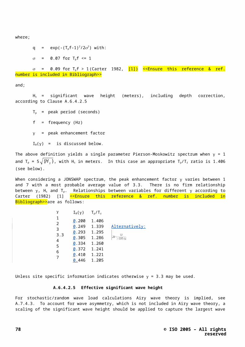
Notes
1) None of these theories is theoretically correct at the breaking limit. Nomenclature
2) Wave theories intended for limiting height waves should be referenced for waves higher than 0.9Hb when stream function theory may underestimate the kinematics.
Hmax/gTass2 = Dimensionless wave steepness
3) Stream function theory is satisfactory for wave loading calculations over the remaining range of regular waves. However, stream function programs may not produce a solution when applied to near breaking waves or deep water waves
d/gTass2 = Dimensionless relative depth
Hmax = Wave height (crest to trough)
Hb = Breaking wave height
d = Mean water depth
4) The order of stream function theory likely to be satisfactory is circled. Any solution obtained should be checked by comparison with the results of a higher order solution.
Tass = Wave period
L = Wave length (distance between crests)
5) The error involved in using Airy theory outside its range of applicability is discussed in the background document.
g = Acceleration due to gravity
Figure A.7.3-5 — Range and validity of different wave theories for regular waves, (after HSE [3]) <<Be sure to capture reference and reference number in bibliography>>
© ISO 2005 – All rights reserved 83

A.7.3.3.5 Stochastic waves
Stochastic analysis may be performed in the frequency or in the time domain.
In a frequency domain analysis linearization assumptions are considered with respect to wave and current loading, as well as for structural and soil non-linearities. Frequency domain analysis should thus be performed only in case of moderate wave conditions with structural or soil non-linearities of small significance, or when proper linearization may be performed. Generally, time domain analysis is recommended for stochastic wave jack-up analysis.
In a stochastic time domain analysis the waves are modelled as a linear random superposition model which is fully described by the wave spectrum, (see A.6.4.2.4, A.6.4.2.5, A.6.4.2.6, and A.4.2.7). It is recommended that the random seastate is generated from the summation of at least 200 component Linear (Airy) waves of height and frequency determined to match the required wave spectrum. The phasing of the component waves should be selected at random.
The extrapolation of the wave kinematics to the free surface is most appropriately carried out by substituting the true elevation at which the kinematics are required with one which is at the same proportion of the still water depth as the true elevation is of the instantaneous water depth. This can be expressed as follows:
z' =
where;
z' = The modified coordinate to be used in particle velocity formulationz = The elevation at which the kinematics are required (coordinate measured vertically upward
from the still water surface) = The instantaneous water level (same axis system as z)d = The still, or undisturbed water depth (positive).
This method ensures that the kinematics at the surface are always evaluated from the linear wave theory expressions as if they were at the still water level, Wheeler (1969) [4] <<be sure to capture reference and reference number for bibliography>> <<see B5-5 Figure C4.4.2 in the Commentary). >>
The statistics of the underlying random wave process are gaussianGaussian and fully known theoretically. The empirical modification around the free surface to account for free surface effects, together with the fact that drag loads are a nonlinear (squared) transformation of wave kinematics, makes the hydrodynamic load excitation always nonlinear. As a result, the random excitation is non-gaussianGaussian. The statistics of such a process are generally not known theoretically, but the extremes are generally larger than the extremes of a corresponding gaussianGaussian random process. For a detailed investigation of the dynamic behaviorbehaviour of a jack-up the non-gaussianGaussian effects must be included. A number of procedures for doing this are presented in the <<Annex C Commentary>>.
When the random displacements of the submerged parts are small and the velocities are significant with respect to the water particle velocities the damping is not well represented by the relative velocity formulation in Morison's equation, which will tend to overestimate the damping and under predict the response. A criterion for determining the applicability of the relative velocity formulation is given in A.7.3.3.2.
A summary of recommendations for frequency and time domain modelling of random waves is given in Table A.7.4-23.4.
84 © ISO 2005 – All rights reserved

Table A.7.3-4 - Recommendation for modelling of frequency and time domain stochastic wavesMethod Recommendations
Frequency Domain
Consider linearization assumptions with respect to:
- wave-current loading (quadratic dependence on particle velocity and finite wave ht).
- structural non-linearity.
Generate random sea from at least 200 components and use divisions of equal frequency.
Note: Fewer frequency components may be used provided that the divisions are shown to be sufficiently small around the wave period, the natural period and periods associated with reinforcement and cancellation.
Time Domain
Generate random sea from at least 200 components and use divisions of generally equal energy. It is recommended that smaller energy divisions are used in the higher frequency portion of the spectrum, which will generally contain the reinforcement and cancellation frequencies. Each wavelet should be taken to disperse with its own linear dispersion relationship [9]. <<be sure to capture reference and reference number for bibliography>>
Check validity of wave simulation:
- correct mean wave elevation
- standard deviation = (Hs/4) 1%
- - 0.03 < skewness < 0.03
- 2.9 < kurtosis < 3.1
- Maximum crest elevation = (Hs/4) -5% to +7.5%
where N is the number of cycles in the time series being qualified,
N Duration / Tz
Integration time-step less than the smaller of:
Tz/20 or Tn/20
where
Tz =the zero-upcrossing period of the wave spectrum
Tn = the jack-up natural period
(unless it can be shown that a larger time-step leads to no significant change in results)
Avoid transients in 'run-in' ( 100 secs).
Ensure simulation length OK for method chosen to determine the Most Probable Maximum Extreme (MPME) response(s) <<Reference to definition – like MPME is defined in Table 7.3>>
© ISO 2005 – All rights reserved 85

A.7.3.3.6 Directionality and spreading
The effects of directionality and wave spreading may be considered in any random dynamic analysis. It is recommended that a comparison be made between the Base Shear Transfer Function (BSTF) for the chosen 2-D (long crested/unspread) analysis direction and the 3-D (short crested/spread) BSTF to determine whether the selected direction is unconservative. Optimally the direction of the 2-D seastate should be chosen to obtain a match with the 3-D BSTF for the entire wave spectrum. If this is not possible the match between the spread and unspread BSTFs should be good at the natural period.
A 3-D BSTF, H3D, can be generated from a set of 2-D BSTFs, H2D, by the following expression:
H3D() =
where:
= Wave excitation frequency
= Angle between 2-D BSTF and dominant direction of 3-D BSTF
n = Power constant of spreading function
2.0 for fatigue analysis
4.0 for extreme analysis
A simple approximation to the incorporation of wave spreading into inertial load calculations is to perform a 2-D analysis with the wave approach angle which is between the two approach angles which give the maximum and minimum forces at the cancellation and reinforcement points (see Figure ?? in Informative Annex C).
<< Review Panel Feb 06 : Add a note giving a simple explanation of the issue and possibly a simplified approach >>
A.7.3.3.7 Current
The current velocity and profile as specified in A.6.4.3 should be used. Interpolation between the data points may be required and liWhere the current profile is defined by discrete points linear interpolation between the data points is recommended sufficientfor simplicity.
The current induced drag forces are to be determined in combination with the wave loads. This is to be carried out by the vectorial addition of the wave and current induced particle velocities prior to the drag load calculations.
The current may be reduced due to interference from the structure on the flow field of the current, Taylor [5]. ] <<be sure to capture reference and reference number for bibliography>> The current may be reduced as follows (see B5-5 Commentary):
VC = Vf [1 + CDeDe/(4D1)]-1
where;
VC = the current velocity to be used in the hydrodynamic model, VC should be not taken as less than 0.7Vf.
Vf = the far field (undisturbed) current.
CDe = equivalent drag coefficient, as defined in A.7.3.3.
De = equivalent diameter, as defined in A.7.3.3.
86 © ISO 2005 – All rights reserved

D1 = face width of leg, outside dimensions.
A.7.3.4 Wind loads
A.7.3.4.1 Wind load
The wind force for each component (divided into blocks of not more than 15m vertical extent), F Wi, may be computed using the formula:
FWi = Pi AWi
where;
Pi = the pressure at the center of the block.AWi = the projected area of the block considered.
The pressure Pi should be computed using the formula:
Pi = 0.5 Vzi2 Cs
where;
= density of air (to be taken as 1.2224 kg/m3 unless an alternative value can be justified for the site).
Vzi = the specified wind velocity at centre of each block A.6.4.6.2.
Cs = shape coefficient, as given below.
NOTE The wind area of the hull and associated structures (excluding derrick and legs) may normally be taken as the profile area viewed from the direction under consideration.
A.7.3.4.2 Shape coefficient
Using a building block of elements the following shape coefficients should be used :
Type of member orStructure
Shape coefficientCs
Hull side, (flat side). 1.0, based on total projected area.
Deckhouses, jack-frame structure, sub-structure, draw-works house, and other above-deck blocks.
1.1, based on the total projected area (i.e. the area enclosed by the extreme contours of the structure)
Leg sections projecting above jack-frame structure and below the hull.
Cs = CDe as determined from A.7.3.4 using tubular CDI = 0.5 AWi determined from De and section length.
Isolated tubulars (crane pedestals, etc.) 0.5
Isolated structural shapes (angles, channels, box, I- sections).
1.5, based on member projected area.
Derricks, crane booms, flare towers (open lattice sections only, not boxed- in sections.)
The appropriate shape coefficient for the members concerned applied to 50% of the total projected profile area of the item (25% from each of the front and back faces).
Shapes or combinations of shapes which do not readily fall into the above categories will be subject to special
© ISO 2005 – All rights reserved 87

consideration.
A.7.3.4.3 Wind tunnel data
Wind pressures and resulting loads may be determined from wind tunnel tests on a representative model when wind loads are crucial.
A.7.4 Functional loads
Provided appropriate procedure exist and it is practical to change the mode of the jack-up unit from operating to elevated storm mode on receipt of an unfavourable weather forecast, only the elevated storm condition need be assessed. Consideration should be given to loadings on the conductors if supported by the jack-up.
The following should be defined:
a) Maximum and minimum elevated weight and weight distribution (fixed and variable load). In the absence of other information the minimum elevated weight may normally be determined assuming 50% of the variable load permitted by the operating manual.
b) Extreme limits of centre of gravity position (or reactions of the elevated weight on the legs) for the conditions in a) above.
c) Substructure and derrick position, hook load, rotary load, setback and conductor tensions for the conditions in a) above.
d) Weight, centre of gravity and buoyancy of the legs.
If a minimum elevated weight or a limitation of center of gravity position is required to meet the overturning acceptance criteria (see Clause 13.x.x), then the addition of water in lieu of variable load is permitted, provided that:
a) Maximum allowable loadings are not exceeded.
b) Procedures, equipment and instructions exist for performing the operation.
c) The maximum variable load, including added water, is used for all appropriate assessment checks (preload, stress, etc.).
If a reduction in elevated weight or a limitation of center of gravity position is required to meet the foundation acceptance criteria (see Clause 13.x.x), then the variable load may be limited provided that procedures, equipment and instructions exist for the timely performance of the operation.
<< Do we need the following one-line paragraphs? Can we point directly to the destination from the tables ?? >>>
A.7.5 Displacement dependent loads
The effect of large displacement, i.e. (P-delta) should be considered as described in A.8.7.3.
A.7.6 Dynamic effects
Further information on dynamic modelling of dynamic loads is given in A.10.5.2 and A.10.5.3. xx?? >>.
A.7.7 Earthquake
Procedures for developing earthquake loads are contained in 10.7
88 © ISO 2005 – All rights reserved

A.7.8 Other Loads
Other loads should be represented as relevant for the site.
For areas where accumulation of ice may occur in the season for the planned operation the possible effect on weight and the environmental loads should be considered. Relevant data for the region should be applied. For calculating wave, current and wind actions, increases in dimension and changes in shape and surface roughness may be of significance.
© ISO 2005 – All rights reserved 89

A.8 Structural modelling
A.8.1 ScopeApplicability
This clause outlines, in some detaildescribes, methods for the development of an analytical model of an independent leg jack-up. Techniques for modelling of the legs, hull, leg/hull connection, and leg/spudcan connection are discussed. Modelling of the The leg/hull connection model includes the upper and lower guides, jacking pinions, fixation systems, and jackcase/ and associated bracing is also discussed. Modelling of the foundation is not consideredlimited to the structural details in this clause;, geotechnical aspects arebut is presented in A.9.
A.8.2 General Overall considerations
A.8.2.1 General
No guidance offered
A.8.2.2 Modelling philosophy
For most jack-up configurations the load distribution at the leg-hull interface is not amenable to manual calculation so a Finite Element (FE) computer model is required. The structural model should accurately reflect the complex mechanism of the jack-up. so, for most jack-up configurations, this requires the use of a Finite Element (FE) computer model. It is most desirable to fully model the jack-up when assessing its structural strength. Very often assumptions and simplifications such as equivalent hull, equivalent leg, etc. will be made in the process of building the model.
A.8.2.3 Levels of FE modelling
While it can be considered desirable to fully model the jack-up when assessing its structural strength this is rarely necessary for a site assessment. An overly complex model can introduce errors and unnecessarily complicate the assessment. Consequently assumptions and simplifications such as equivalent hull, equivalent leg, etc. are often made when building the model(s) used for the assessment.Assumptions and simplifications may be made in the process of building the model. In view of this, various levels of modelling described in a) through d) below may can be used. It should be noted that some of these methods may have limitations with respect to the accuracy of assessing the structural adequacy of a jack-up. Table A 8.2-1 outlines the limitations of the various modelling techniques and should be referenced to ensure that the selected model addresses all aspects required for the assessment. When simplified models, such as those described in (b) and (d), are used, it may beis usually appropriate to calibrate them against a more detailed model.
<< The cross-referencing in the following paras needs further thought >>
a) Fully detailed leg model
The model consists of 'detailed legs', hull, hull/leg/hull connections and spudcans modelled in accordance with A.8.3.2, A.8.4.2, 8.5, A.8.5 and A.8.6, respectively. The results from this model can be used to examine all aspects of a jack-up site assessment including foundation stability requirements, overturning resistance, leg strength and the adequacy of the jacking system or fixation system.
90 © ISO 2005 – All rights reserved

Figure A.8.2-1- Combined equivalent/detailed leg and hull model
b) Equivalent stick-leg model(stick model)
The model consists of 'equivalent 'stick modellegs' legsmodelled in accordance with A.8.3.3, hull structure modelled using beam elements in accordance with A.8.4.3, leg to hull connections modelled in accordance with A.8.5 and spudcans modelled as a stiff or rigid extension to the equivalent leg. The results from this model can be used to examine foundation stability requirements and overturning resistance. This model may also be used to obtain reactions at the spudcan and internal forces and moments in the leg at the vicinity of the lower guide for application to the 'detailed leg' and leg/hull model (d) which should be used to assess the strength of the leg in the area between lower and upper guides.
c) Combined equivalent/detailed leg and hull model
The model consists of a combination of 'detailed leg' for the upper portion of legs and 'equivalent 'stick leg' model' for the lower portion of the legs modelled in accordance with A.8.3.4. The hull, leg/hull connections and spudcans are modelled in accordance with A.8.4, A.8.5 and A.8.6 respectively. The results from this model can be used to examine foundation stability requirements, overturning resistance, leg strength in the region of the leg/hull connections and the adequacy of the jacking and/or fixation systems.
d) Detailed single leg and leg/hull connection model
The model consists of a 'detailed leg' or a portion of a 'detailed leg' modelled in accordance with A.8.3.2, the leg/hull connection modelled in accordance with A.8.5 and, when required, the spudcan modelled in accordance with A.8.6. The results from this model can be used to examine the leg strength and the adequacy of the jacking and/ or fixation systems.
© ISO 2005 – All rights reserved 91

Table A 8.2-1 — Applicability of the suggested models
Applicability
ModelType
I
GlobalLoads
II
OverturningChecks
III
FoundationChecks
IVGlobalLegLoads
VLegMemberLoads
VIJacking / FixationSystem oads
VIIHullElementLoads
a) Fully detailed leg Y Y Y Y Y Y See note1
b) Equivalent leg (stick model) Y Y Y Y - - -
c) Combined equivalent / detailed leg and hull
Y Y Y Y Y Y See note1
d) Detailed single leg and leg/hull connection model
- - - - Y Y -
Legend:
Y = Applicable
- = Not applicable
Notes:
1) Hull stresses will only be available from more complex hull models.
A.8.3 Modelling the leg
A.8.3.1 General
The For truss legs the model(s) shall may be generated in accordance with the applicable following sub-clause(s). Single column legs may modelled either in accordance with A.8.3.3 or by means of appropriate non-beam finite elements << P3 to review this >>.
A.8.3.2 Detailed leg
Modelling should account for offsets between element work points and centroids as omitting this detail may can be non-conservative. If member offsets are not included in the model, analysis of the relevant joints should consider this their effect. Gusset plates may be ignored in the structural leg model. However their effects may be taken into account in the calculation of member and joint strength.
A.8.3.3 Equivalent stick leg (stick model)
The leg structure can be simulated by a series of collinear beams with the equivalent cross sectional properties calculated using the formulae indicated in Figure A.8.3-1 or derived from the application of suitable 'unit' load cases to the 'Detailed Leg'. The stiffness properties of the equivalent leg shall equate to those of the ‘detailed leg’ model described above. The simplified formulae indicated below may be used to calculate stiffness properties. Where such a model is used, analysis results must be combined with a detailed leg model to determine member stresses, fixation system/pinion loads, etc.
The determination of stiffness for the equivalent leg model referred to above may be accomplished as outlined below:
Equivalent leg stiffness
Hand calculations using the formulae presented in Figure A.8.3-1. Provided that there are no significant offsets between the brace work points these will be reasonably accurate for cases A (sideways K bracing), C (X bracing) and D (Z bracing); case B (normal K bracing) should be used with caution as the values of
92 © ISO 2005 – All rights reserved

equivalent shear area and second moment of area are dependent on the number of bays being considered. If the leg scantlings change in different leg sections this can be accounted for by calculating the properties for each leg section and creating the equivalent leg model accordingly.
The application of unit load cases to a detailed leg model prepared in accordance with 8.3.2 and 8.3.5 and rigidly restrained at the first point of lateral load transfer between the hull and leg. The following load cases should be considered, applied about the major and minor axes of the leg:
- Axial load. This is used to determine the axial area, A, of the equivalent beam according to standard theory:
where;
= axial deflection of cantilever at point of load application
F = applied axial end load
L = cantilevered length (from rigid support to seabed reaction point – see A.8.6.2)
E = Young's modulus
‘Rigid support’ is considered to be the first point of lateral load transfer between the hull and leg
<< should consider this - the analyst may find it more convenient to use a different reference point e.g chock level or neutral axis of hull >>.
- Pure moment applied either as a moment or a couple. This is used to derive the second moment of area (I) according to standard beam theory:
and
where;
= lateral end deflection of cantilever at point of load application
M = applied end moment
= end slope of cantilever at point of load application
It should be noted that the value of I resulting from the two equations may can differ somewhat.
- Pure shear, P, applied at the end of the leg which may be used to derive I according to standard beam theory:
Using either this value of I, or a value obtained from the pure moment case, the effective shear area, As, can then be determined from:
© ISO 2005 – All rights reserved 93

where;
G = shear modulus = E/2.6 for Poisson’s ratio of 0.3
A.8.3.4 Combination detailed and equivalent stick leg
The combined detailed and equivalent stick leg model shall be constructed with the areas of interest being modelled in detail and the remainder of the leg is modelled as an equivalent legstick. To facilitate obtaining detailed stresses in the vicinity of the leg/hull connection (guides, fixation/jacking system, etc.), the detailed portion of the leg model should extend far enough above and below this region to ensure that boundary conditions at the ‘detailed leg’/‘equivalent leg’ connection do not affect stresses in the areas of interest. Care is required to ensure an appropriate interface and consistency of boundary conditions at the connections.
The plane of connection between ‘detailed leg’/‘’equivalent leg’ should remain a plane and without shear distortion when the leg is bent. The connection should be composed of rigid elements that control local bending and shear distortion.
A.8.3.5 Stiffness adjustment
No Guidance is offered
A.8.3.6 Leg inclination
No guidance offered
A.8.4 Modelling the hull
A.8.4.1 General
Recommended methods of modelling the hull structure are given in the following sub-clauses:
A.8.4.2 Detailed hull model
The model shall be generated using plate elements in which appropriate directional modelling of the effect of the stiffeners on the plates shall be included. The elements shall be capable of carrying in-plane and, where applicable, out of plane loads.
A.8.4.3 Equivalent hull model
The deck, bottom, side shell and major bulkheads are modelled as a grillage of beams in an equivalent hull model. The properties of the beams should be calculated based on the depth of the bulkheads, side-shell and the ’effective width’ of the deck and bottom plating. Beam elements should be positioned with their neutral axes at mid-depth of the hull. Attention should be paid to the in-plane and torsional properties due to the continuity of the deck and bottom structures. << calculate torsional property of box and divide amongst the grillage members>>
. << This sub-clause could be usefully expanded - mass distribution & yaw gyradius >>
A.8.5 Modelling the hull/leg/hull connection
A.8.5.1 General
The leg/hull connection modelling is of extreme importance to the analysis since it controls the distribution of leg bending moments and shears carried between the upper and lower guide structures and the jacking or fixation system. It is therefore necessary that these systems are properly modelled in terms of stiffness, orientation and clearance. For the equivalent stick-leg model a simplified derivation of the equivalent leg/hull connection stiffness may be applicable.
94 © ISO 2005 – All rights reserved

A specific jack-up design concept can be described by a combination of the following components (see also Figure A.8.5-1):
a) With or without fixation system,
b) Opposed or unopposed jacking pinions,
c) Fixed or floating jacking system.
F ixe djack in gsys tem
Flo atin gjac k in gs ys tem
O p p osed p in io n s
F ix edjac k in gs ys te m
Floa tin gjack in gs ys te m
U n op p o se d p in ion s
F ix at ion s y stem
Fixedjac k in gs ys tem
F loa tingja ck ings ys tem
O p po s ed p in ion s
F ixe dja ckin gs ystem
F lo atin gjac kin gsy st em
U n op p os ed p in io n s
N o fi xat io n s ys te m
L E G -H UL L C O N NE C TIO N
F&G L 780 II MSC CJ 46
L780 V, L780 VI MSC CJ 50
Hitachi giant
MSC CJ 62
Modec 300c MSC CJ 50 LeTourneau
CFEM 2005 -116C
CFEM 2600 -Super 300
Gusto -Gorilla
Examples of
Units in this
category
MSC CJ50 is not floating; Gustos are in other categories …
Figure A.8.5-1- Leg/hull connection component combinations
<< suggest that the moment carrying mechanisms (vertical and horizontal force couples) are explained in more detail (diagrams?). Also need to advise that some units with fixation systems release the pinions >>
For jack-ups with a fixation system, the leg bending moment will be shared by the upper and lower guides, the jacking and the fixation systems. Normally the leg bending moment and axial force due to environmental loading are resisted largely by the fixation system because of its high rigidity. Depending on the specified method of operation, the stiffnesses, the initial clearances and the magnitude of the applied loading a portion of the environmental leg loading may can be resisted by the jacking system and the guide structures. Typical shear force and bending moment diagrams for this configuration are shown in Figure A.8.5-2.
For jack-ups without a fixation system, the leg bending moment will be shared by the jacking system and guide structure. For a fixed jacking system, the distribution of leg moment carried between the jacking system and guide structure mainly depends on the stiffness of the jacking pinions. Typical shear force and bending moment diagrams for this configuration are shown in Figures A.8.5-3 and A.8.5-4.
For a floating jacking system, the distribution of leg bending moment carried between the jacking system and guide structure depends on the combined stiffness of the shock pads and pinions. Typical shear force and bending moment diagrams for this configuration are shown in Figure A.8.5-5.
The leg/hull connection should be modelled considering the effects of guide and support system clearances, wear, construction tolerances and backlash (within the gear-train and between the drive pinion and the rack).
© ISO 2005 – All rights reserved 95

If the jacking system has unopposed pinions, local chord moments will arise due to:
The horizontal pinion load component (due to the pressure angle of the rack/pinion).
The vertical pinion load component acting at an offset from the chord neutral axis.
The following techniques are recommended for modelling leg/hull connections (specific data for the various parts of the structure may can be available from the design data package):
Add SNAME sketches of opposed & unopposed pinions
A.8.5.2 Guide Systems
The guide structures shall be modelled to restrain the chord member horizontally only in directions in which guide contact occurs. The upper and lower guides may be considered to be relatively stiff with respect to the adjacent structure, such as jackcase, etc. The nominal lower guide position relative to the leg may can be derived using the sum of leg penetration, water depth and airgap. It is however recommended that at least two positions are covered when assessing leg strength: one at a node and the other at midspan. This is to allow for uncertainties in the prediction of leg penetration and possible differences in penetration between the legs.
The finite lengths of the guides may be included in the modelling by means of a number of discrete restraint springs/connections to the hull. Care is required to ensure that such restraints carry loads only in directions/senses in which they can act. Alternatively the results from analyses ignoring the guide length may be corrected, if necessary, by modification of the local bending moment diagram to allow for the proper distribution of guide reaction, see Figure A.8.5-6.
A.8.5.3 Elevating system
A.8.5.3.1 Jacking (or elevating) pinions
The jacking pinions shall be modelled based on the pinion stiffness specified by the manufacturer and should be modelled so that the pinions can resist vertical and the corresponding horizontal forces. A linear spring or cantilever beam can be used to simulate the jacking pinion. The force required to deflect the free end of the cantilever beam a unit distance should be equal to the jacking pinion stiffness specified by the manufacturer. The offset of the pinion/rack contact point from the chord neutral axis should be incorporated in the model.
A.8.5.3.2 Other
<< P3 to add text re other types of elevating systems - model the stiffness >>
A.8.5.4 Fixation system
The fixation system shall be modelled to resist both vertical and horizontal forces based on the stiffness of the vertical and horizontal supports and on the relative location of their associated foundations. It is important that the model can simulate the local moment capacity of the fixation system arising from its finite size and the number and location of the supports.
A.8.5.5 Shock pad – floating jacking systems
Floating jacking systems generally have two sets of shock pads at each jackcase, one located at the top and the other at the bottom of the jackhouse. Alternatively shock pads may can be provided for each pinion or block of pinions. The jacking system is free to move up or down until it contacts the upper or lower shock pad. In the elevated condition, the jacking system is in contact with the upper shock pad and in the transit condition it is in contact with the lower shock pad. The stiffness of the shock pad should be based on the manufacturer's data and the shock pad should be modelled to resist vertical force only. It should also be noted that the shock pad stiffness characteristics may beare normally nonlinear.
96 © ISO 2005 – All rights reserved

A.8.5.6 Jackcase and associated bracing
The jackcase and associated bracing should be modelled based on the actual stiffness since it has direct impact on the horizontal forces that the upper guide can resist.
If the hull is not modelled it is normally suitable to restrain the base of the jackcase and associated bracing, the foundations of the fixation system and the lower guide structures at their connections to the hull.
A.8.5.7 Equivalent leg/hull stiffness
The determination of stiffnesses for the equivalent leg/hull connection model referred to in 8.5.7 may be accomplished the following means:
Hand calculations using the formulae presented in Figure A.8.3-1
The application of unit load cases to a detailed leg model in combination with a detailed leg/hull connection model in accordance with 8.3.2 and 8.5. Unit load cases are applied, as described in A.8.3.3. In this instance the differences between the results from the detailed leg model alone (see A.8.3.3) and the detailed leg plus leg/hull connection model allow the effective stiffness of the connection to be determined:
Axial load. This is used to determine the vertical leg/hull connection stiffness, Kvh from the axial end displacements of the detailed leg model, , and the axial end displacements of the combined leg and leg/hull connection model, C, under the action of the same loading, F:
Kvh = F/(C-)
Pure moment applied either as a moment or a couple. This is used to derive the rotational connection stiffness, Krh from either the end slopes, and C, or the end deflections, and C, of the two models under the action of the same end moment, M:
Krh = M/(C-) or Krh = ML/(C-)
Pure shear which may can be used to determine the horizontal leg/hull connection stiffness, Khh, in a similar manner, accounting for the rotational stiffness already derived. Normally the horizontal leg/hull connection stiffness may be assumed infinite.
If the model contains nonlinearities due to the inclusion of gap elements care should be taken to ensure that suitable levels of 'unit' loading are applied such that the derived stiffness is applicable to the analysis to be undertaken.
A.8.6 Modelling the spudcan and foundation
A.8.6.1 Spudcan structure
When modelling the spudcan, rigid beam elements are considered sufficient to achieve an accurate load transfer of the seabed reaction into the leg chords and bracing in the area between upper and lower guides. It should be noted that, due to the sudden change in stiffness, these rigid beams may can cause artificially high stresses at the leg to spudcan connections. Hence the modelling and selection of element type should be carefully considered when an accurate calculation of leg member stresses is required in this area.
For a strength analysis of the spudcan and its connections to the leg it may can be appropriate to develop a separate detailed model with appropriate boundary conditions.
A.8.6.2 Seabed reaction point
The vertical position of the reaction point at each spudcan shall be located at a distance above the spudcan tip equivalent to:
© ISO 2005 – All rights reserved 97
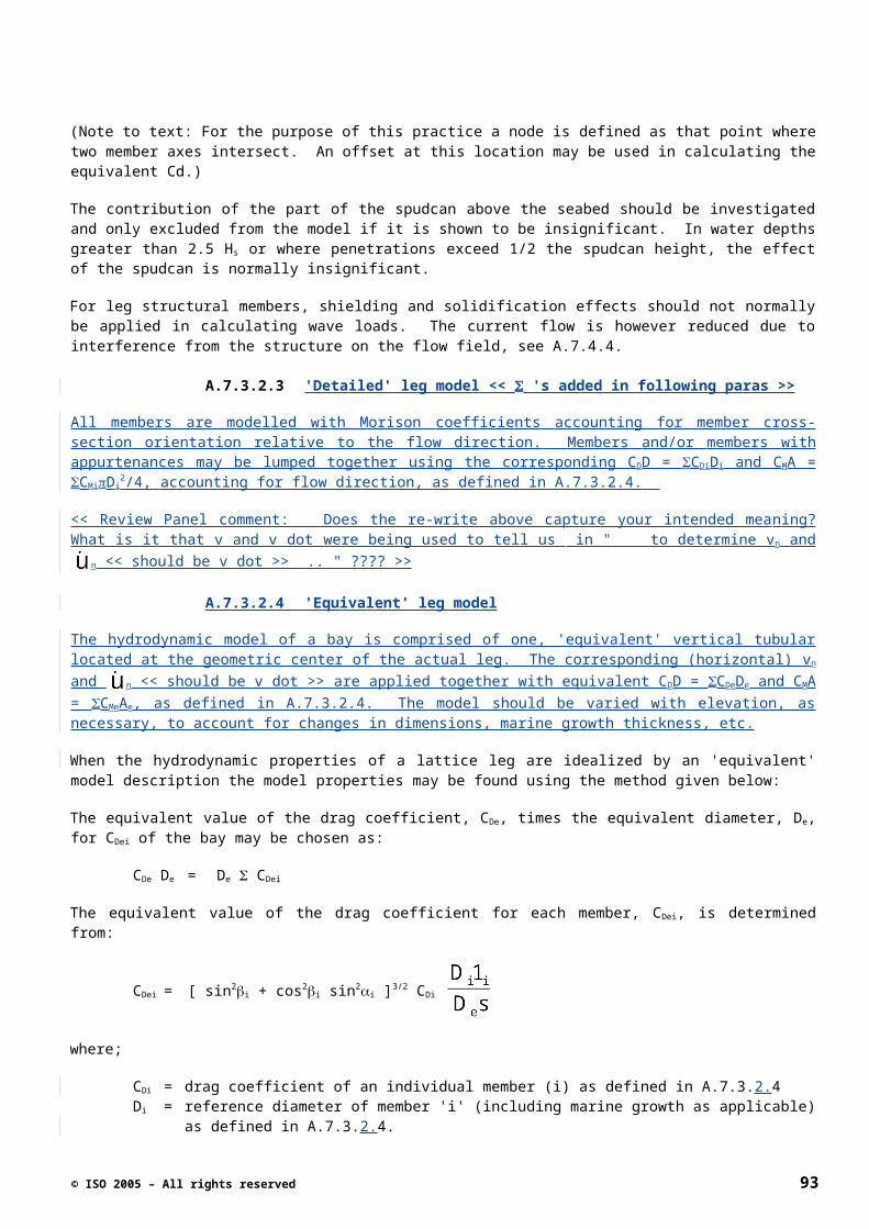
a) Half the maximum predicted penetration (when spudcan is partially penetrated), or
b) Half the height of the spudcan (when the spudcan is fully penetrated)
c) If detailed information exists regarding the soils and spudcan the position of the reaction point may be calculated. (Brekke et al)<<should this be referenced in the foundation section – check with Panel 4???>>
The legs of an independent leg jack-up will normallymay be assumed to be pinned at the reaction point. Any divergence from this assumption should be clearly stated together with the assumptions for any moment fixity provided to the leg's cans by the soil.
The horizontal position (eccentricity) of the reaction point used in the analysis shall be established through consideration of spudcan geometry and seabed topology under the action of preload.
Non-symmetrical geometries shall be specially considered.
Note: Situations leading to horizontal eccentricity may can result from spudcan geometry, sloping seabeds, bottom obstructions, existing spudcan holes, etc.
Further discussion on seabed reaction is contained in Clause 9.
A.8.6.3 Foundation modelling
Methods of establishing the degree of rotational restraint, or fixity, at the footings are discussed further in Clauses 9 and A.9. Upper or lower bound values should be considered as appropriate for the areas of the structure under consideration.
For checking the spudcans, the leg-to-can connection and the lower parts of the leg, appropriate calculations considering soil-structure interaction shall be carried out to determine the upper bound spudcan moment. These areas may be checked assuming that a percentage of the maximum storm leg moment at the lower guide (derived assuming a pinned footing) is applied to the spudcan together with the associated horizontal and vertical loads. This percentage would normally be not less than 50%. For such simplified checks the loading on the spudcan may be modelled assuming that the soil is linear-elastic and incapable of taking tension.
A.8.7 Mass Modelling
No guidance offered.Refer to A.8.8.2. << may be better to bring (or repeat) the key thoughts together here >>
A.8.8 Application of loads actions and load action effects
A.8.8.1 General
The loads and load effects to be included in the analysis comprise of:
a) Self weight and non-varying loads, variable and drilling loads.
b) Wind loads.
c) Hydrodynamic wave-current loads.
d) Inertial loads due to dynamic response.
e) Second order effects.
The assessment follows a partial factor format. The partial action factors are applied to actions as defined in other clauses (i.e. they are action factors, NOT action-effect factors).
These loads and load effects are discussed in turn below.
98 © ISO 2005 – All rights reserved

A.8.8.2 Permanent and variable loads
To correctly capture these effects the hull loads should be applied to the model in such a manner as to represent their correct vertical and horizontal distribution. If dynamic analyses are to be performed all weights should be represented by means of masses together with vertical gravitational acceleration. It is generally appropriate to apply these masses by means of factored element self-weight with additional correction masses applied as necessary to obtain the correct total mass and centre of gravity. Alternatively, it may be sufficient to apply point masses at the node points of the model.
The bulk of the text in the following 2 paragraphs needs to be merged with A.8.8.3
Depending on the initial positions of the legs with respect to guide clearances, and the operation of the jacking and fixation systems (if fitted), the distributed hull loading and stiffness will lead to hull sagging which may can impose bending moments on the legs which remain present for the remainder of the period on site. Such moments should be considered in the site assessment analyses, and will be larger in shallow waters where the leg extension below the hull is small and consequently the leg bending stiffness is higher.
To correctly capture these effects the hull loads should be applied to the model in such a manner as to represent their correct vertical and horizontal distribution. If dynamic analyses are to be performed all weights should be represented by means of masses together with vertical gravitational acceleration. It is generally appropriate to apply these masses by means of factored element self-weight with additional correction masses applied as necessary to obtain the correct total mass and centre of gravity. Alternatively, it may be sufficient to apply point masses at the node points of the model.
It is noted that an F.E. model with distributed hull stiffness and loading will incorporate hull sag effects if the hull and variable gravity loading is 'turned on' with the jack-up defined in its initially undeflected shape at the operating airgap. It should be verified that the amount of hull sag moment arising is applicable, given the operating procedures pertaining to the jack-up. It may be necessary to apply corrections to the final results for any discrepancies in the hull sag induced loadings. Further guidance is given in Clause A.8.7.2.18.3 below << update reference >>.
At some sites, the extreme storm may can be less then the limits specified for operating conditions. Care must be taken to ensure that the site assessment is based on the worst anticipated conditions of loading, i.e. with increased elevated weight, cantilever extended and unequal leg loads.
A.8.8.3 Hull sagging
When a jack-up is installed on site the legs will normally engage the seabed with the hull supported by its own buoyancy in a hogged condition. Subsequently, with the hull slightly clear of the water, preload ballast will be taken on board thus preloading the legs to achieve their final penetration. This will normally lead to an extreme hull sagging condition. Finally the preload ballast is dumped and the hull elevated to the required airgap for the site. In this condition the hull will be sagging under self-weight and variable loads.
As explained in Clause A.8.7.2 above, the leg shear and bending moments caused by hull sagging are very dependent on leg guide clearances, the design of the jacking system, operational parameters and the modelling used in the analysis. A simplified approach for a conservative quantitative assessment is to assume that 25 to 50 percent of the theoretical hull sagging moment at the lower guide is seen in practice. This may be accounted for in a global model by reducing the distributed hull mass by 75 to 50 percent and applying the residual mass as point masses on the hull adjacent to the connections to the legs. This procedure is not applicable when hull stresses are required. A more thorough method is to apply self equilibrating pairs of forces/moments across the spring connections between hull and legs:
© ISO 2005 – All rights reserved 99

An alternative approach is to allow a relaxation of the horizontal seabed restraint by means of prescribed displacements.
A.8.8.4 Environmental loads
A.8.8.4.1 Wind loads
Wind loading is determined from 7.5. The wind loading on the legs above and below the hull shall be modelled to represent the correct vertical and horizontal distribution. Loads may be applied as distributed or nodal loads. Where nodal loads are used, a sufficient number should be applied to reflect the nature of the loading, and it should be ensured that the correct total shear and overturning moment is applied on each leg.
Similarly, the wind loading on the hull and associated structure may be applied as distributed or nodal loads. The application should also ensure the correct total shear and overturning moment is applied to the hull.
A.8.8.4.2 Wave/current loads
Wave/current loading is determined from 7.4. The wave/current loading on the leg and spudcan structures above the mudline should be modelled to represent their correct vertical and horizontal distribution. Where nodal loads are used, their application should ensure the correct total shear and overturning moment on each leg, and reflect the distributed nature of the loading.
A.8.8.5 Inertial loads
When the dynamic approach (see Clause 10) leads to the explicit determination of an inertial loadset, this should be applied to the hull mx`odel. In simpler dynamic approaches the inertial load may be represented by a single lateral point loading acting at the hull center of gravity, or by a number of point loads applied to other parts of the hull having the same line of action. In more complex approaches a more complete distributed load vector may be applied to the hull and legs << Goal is to match BS and OTM >> . << This paragraph lacks the guidance needed to ensure that the modelling is properly representative of the loading e.g. could allow uniformly distributed load over the whole structure >>
A.8.8.6 Large displacement effects
a) Large Displacement Methods
For large displacement methods the solution is obtained by applying the load in increments and iteratively generating the stiffness matrix for the next load increment from the deflected shape of the previous increment.
b) Geometric Stiffness Methods
Geometric stiffness methods apply a linear correction to the stiffness matrix based on the axial load present in the element.
100 © ISO 2005 – All rights reserved

A.8.8.7 Conductor loads
The conductor tension is modelled as a static force; and when applicable, the hydrodynamic loading is included in the jack-up’s global analysis model. An explicit model of the conductor is rarely warranted. Hydrodynamic loading on the conductor can either be modelled as additional loading distributed among the legs, or on an explicit model. The effects of stiffness and damping in the conductor are not generally modelled in a jack-up structural assessment because they are often considered to have negligible influence on the global jack-up response. Structural integrity assessment of an individual conductor is outside the scope of this document.
© ISO 2005 – All rights reserved 101

A.8.8.8 Earthquake loads (see panel 5)
Figure A.8.3-1: Formulas for the determination of equivalent member properties;
(Reference DNV Class Note 31.5 1992 [6] (corrected))
102 © ISO 2005 – All rights reserved
Review panel suggested the figure above and those below could go to TR << BUT NEED TO KEEP Figure A.8.5-6 >>
© ISO 2005 – All rights reserved 103

Figure A 8.5-2: Leg shear force and bending moment - jack-ups with a fixation system
104 © ISO 2005 – All rights reserved

Figure A 8.5-3: Leg shear force and bending moment - jack-ups without a fixation system and having a fixed jacking system with opposed pinions
© ISO 2005 – All rights reserved 105

Figure A.8.5-4: Leg shear force and bending moment - jack-ups without a fixation system and having a fixed jacking system with unopposed pinions
106 © ISO 2005 – All rights reserved

Figure A.8.5-5 Leg shear force and bending moment - jack-ups without a fixation system and having a floating jacking system
© ISO 2005 – All rights reserved 107

Figure A.8.5-6: Correction of point supported guide model for finite guide length
(After DNV Class Note 31.5, 1992 [6]
<< This Figure is/was the same as Fig A.8.3-1 >>
108 © ISO 2005 – All rights reserved

A.9 Foundations
A.9.1 Scope
No guidance offered.
A.9.2 General
The analyses for the stability during assessment loading conditions may be performed using a Working Stress Design (WSD) method with an overall safety factor or a Load and Resistance Factor (LRFD) approach.
<< Following text moved to A.6.5 >>
A.9.2.1 Integrated geoscience studies
Adequate geotechnical and geophysical information shall be available to assess the site and the foundation stability. Aspects, which should be investigated, are shown in Table A.9.2-1 and are discussed in more detail in the referenced sections. The information obtained from the surveys and investigations set out in Clauses A.9.2.1.1 to A.9.2.1.5 is required for areas where there is no data available from previous operations. In areas where information is available, it may be possible to reduce the requirements set out below by use of information obtained from other surveys or activities in the area.
A.9.2.1.1 Bathymetric survey
An appropriate bathymetric survey should be supplied for an area approximately 1 kilometer square centered on the proposed position at the site. Line spacing of the survey should typically be not greater than 100 meters x 250 meters over the survey area. Interlining is to be performed within an area 200 meters x 200 meters centered on the proposed position at the site. Interlining should have spacing less than 25 meters x 50 meters.
A.9.2.1.2 Seabed surface survey
The seabed surface shall be surveyed using sidescan sonar or high-resolution multibeam echosounder techniques and shall be of sufficient quality to identify obstructions and seabed features and should cover the immediate area (normally a 1 km square) of the intended site. The slant range selection shall give a minimum of 100% overlap between adjacent lines. A magnetometer survey may also be required if there are buried pipelines, cables and other metallic debris located on or slightly below the sea floor.
Where seabed obstructions such as pipelines and wellheads are known to be present, sufficient information to enable safe positioning of the jack-up is required. In some cases an ROV or diver’s inspection may be required in addition to the seabed surface survey.
Seabed surface surveys can become out-of-date, particularly in areas of construction/drilling activity or areas with mobile sediments. . At open water sites the maximum period for the validity of seabed surveys for debris and mobile sediment conditions should be determined taking account of local conditions. For positions at the sites (pending Review Panel decision) close to existing installations seabed surveys for debris and sediment conditions should, subject to practical considerations, be undertaken immediately prior to the arrival of the jack-up at the site.
A.9.2.1.3 Shallow seismic survey
The principal objectives of the shallow seismic survey are:
To determine near surface soil stratigraphy. This requires correlation of the seismic data with (existing) soil boring data in the vicinity.
To reveal the presence of shallow gas concentrations.
© ISO 2005 – All rights reserved 109

Due to the qualitative nature of seismic surveys it is not possible to conduct analytical foundation appraisals based on seismic data alone. This requires correlation of the seismic data with soil boring data in the vicinity through similar stratigraphy.
A shallow seismic survey should be performed over an approximately 1 kilometre square area centred on the proposed position at the site. Line spacing of the survey should typically be not greater than 100 meters x 250 meters over the survey area. Equipment should normally be capable of giving detailed data to a depth equal to the greater of 30 meters or the anticipated footing penetration plus 1.5 times the footing diameter.
The survey report should include at least two vertical cross-sections passing through the proposed position at the site showing all the relevant reflectors and allied geological information. The equipment used should be capable of identifying reflectors of 0.5m and thicker.
Geotechnical investigation
Introduction
Site-specific geotechnical investigation and testing are recommended in areas where any of the following apply:
the shallow seismic survey cannot be interpreted with any certainty
no geotechnical data is available in nearby area
significant layering of the strata is indicated
the site is known to be potentially hazardous.
Soil investigation and testing
A geotechnical investigation should comprise a minimum of one borehole to a depth equal to 30 metres or the anticipated footing penetration plus 1.5 times the footing diameter, whichever is the greater. All the layers should be adequately investigated and the transition zones cored at a sufficient sampling rate.
The number of boreholes required should account for the lateral variability of the soil conditions, regional experience and the geophysical investigation. When a single borehole is made, the preferred location is at the center of the leg pattern at the intended position at the site.
“Undisturbed” soil sampling and laboratory testing and/or in-situ piezocone penetrometer testing should be conducted. Other recognized types of in-situ soil testing may be appropriate such as vane shear and/or pressure meter tests.
Geotechnical report
The geotechnical report should include borehole logs, piezocone penetrometer records (if appropriate) and documentation of all laboratory tests, together with interpreted soil design parameters. A competent geotechnical engineer should select design parameters. For the methods recommended in Section 9.3 and 9.4, the design parameters should include profiles of undrained shear strength and/or effective stress parameters, soil indices (plasticity, liquidity, grain size, etc.), relative density, unit weight and, the over consolidation ratio (OCR).
Additional soil testing to provide shear moduli and cyclic/dynamic behaviour may be required if more comprehensive analyses are to be applied or where the soil strength may deteriorate under cyclic loading.
Integrated studies
The results of bathymetric surveys, seabed surface surveys, shallow seismic surveys, seabed samples and geotechnical investigations should be integrated to assess the soil conditions at the proposed site. Lateral variations of geotechnical parameters can be assessed from the correlation of the shallow seismic data and the geotechnical information from the borehole logs or piezocone penetration tests.
110 © ISO 2005 – All rights reserved

Table A.9.2-1 — Foundation risks, methods for evaluation and prevention
RISK
METHODS FOR EVALUATION & PREVENTION SECTION
Installation Problems Bathymetric survey
Seabed surface survey
A.9.2.1.1
A.9.2.2.2
Punch-through Geophysical investigation (shallow seismic survey)
Soil sampling and other geotechnical testing and analysis
A.9.2.1.3
,A.9.3.2.7
Settlement under storm loading/Bearing failure
Geophysical investigation (shallow seismic survey)
Soil sampling and other geotechnical testing and analysis
Ensure adequate jack-up preload capability
A.9.2.1.3
A.9.3.2.7
A.9.3.3
Sliding failure Geophysical investigation (shallow seismic survey)
Soil sampling and other geotechnical testing and analysis
Increase vertical footing reaction
Modify the footings
A.9.2.1.3
A.9.3.3.2
Scour Bathymetric and seabed surface survey (identify sand waves)
Surface soil samples and seabed currents
Inspect footing foundation regularly
Install scour protection (gravel bag/artificial seaweed) when anticipated
A.9.2.1.1
A.9.2.1.2
9.3.4.3
Geohazards (mudslides, mud volcanos etc)
Seabed surface survey
Shallow seismic survey
Soil sampling and other geotechnical testing and analysis
A.9.2.1.2
A.9.2.1.3
Error: Reference source not found
Gas pockets/Shallow gas Geophysical Investigation (shallow seismic survey)
A.9.2.1.3
Faults Geophysical Investigation(shallow seismic survey)
A.9.2.1.3
Metal or other object, sunken wreck, anchors, pipelines etc.
Magnetometer and seabed surface survey A.9.2.1.2
Local holes (depressions) in seabed, reefs, pinnacle rocks, non-metallic structures or wooden wreck
Seabed surface survey
Diver/ROV inspection
A.9.2.1.2
Legs stuck in mud Soil sampling and other geotechnical testing and analysis
A.9.2.1.3
© ISO 2005 – All rights reserved 111

Consider change in footings
Jetting/Airlifting
Eccentric spudcan reactions Bathymetric and seabed surface surveys
Geophysical Investigation (buried channels or footprints)
Soil sampling and other geotechnical testing and analysis
Seabed modification
A.9.2.2.1, A.9.2.2.2
A.9.2.2.3
A.9.2.2.4
Seabed slope Bathymetric and Seabed surface surveys
Seabed modification
A.9.2.2.1, A.9.2.2.2
Footprints of previous jack-ups Evaluate site records
Prescribed installation procedures
Consider filling/modification of holes as necessary
A.9.2.1.1A.9.2.1.2
9.4.1
112 © ISO 2005 – All rights reserved

A.9.3 Geotechnical analysis of independent leg foundations
A.9.3.1 General
This clause addresses the foundation analysis of spudcan supported jack-ups. For mat supported jack-ups see Clause A.9.4 Geotechnical Analysis of Mat Foundations.
(Proper intro to be inserted – P4) Inside the yield surface the foundation behaviour is considered to be elastic, whereas on the yield surface the foundation can undergo inelastic deformation. When the foundation is considered as pinned, the yield surface degenerates to a vertical-horizontal load space. (Richard Dean)
A.9.3.2 Leg penetration during preloading
A.9.3.2.1 Introduction
The majority of spudcans are effectively circular in plan but other spudcan geometries are not uncommon. The bearing capacity formulas given in this section are consistent with 'circular' spudcan footingspudcans without skin-friction on the leg. Due consideration should be given to the tapered geometry of most spudcans for bearing capacity assessment.
Note: Terms which are not defined in the text may be found in Clause A4.9.
Figure A.9.3-1 — Typical spudcan geometries
© ISO 2005 – All rights reserved 113

Figure A.9.3-2 — Spudcan foundation model
114 © ISO 2005 – All rights reserved

A.9.3.2.2 Analysis method
The conventional procedure for the assessment of spudcan load/penetration behaviour is given in the following steps:
1. Model the spudcan.
2. Compute the vertical bearing capacity of the footing at various depths below seabed using closed form bearing capacity solutions and plot as a curve to suitable depth.
3. Enter the vertical bearing capacity versus footing spudcan penetration curve with the specified maximum vertical installation (during preloading) reaction at the footingspudcans and read off the predicted footing spudcan penetration.
For conventional foundation analyses the spudcan can often be modelled as a flat circular foundation. The equivalent diameter is determined from the area of the actual spudcan cross section in contact with the seabed surface, or where the spudcan is fully embedded, from the largest cross sectional area in plan. Foundation analyses are then performed for this circular foundation at the depth (D) of the maximum cross sectional area in contact with the soil. Conical shapes are discussed in Annex D. Alternative shapes, e.g. tubular legs, should be treated as appropriate.
The depth of spudcan penetration is often defined as the distance from the spudcan tip to the mudline. In the analytical model below the depth D is defined as the depth of the maximum diameter of the spudcan below mudline. It is therefore necessary to correct for this when referring to the analytical foundation model.
The possibility of soil back-flow over the footing spudcan should be considered when computing bearing capacity. In very soft clays complete back-flow may occur whereas in firm to stiff clays and granular materials, where limited footingspudcan penetration may be expected, the significance of back-flow diminishes. The effect of punch through or local failure of a weak layer between two stronger layers, e.g. squeezing, should be incorporated in the soil model underneath the footingspudcan.
A.9.3.2.3 Penetration in clays
The ultimate vertical bearing capacity of a foundation in clay of uniform shear strength (undrained failure in clay, = 0) at a specific depth can be expressed by:
FV = (cu.Nc.sc.dc + po')A.
For the selection of the design undrained shear strength su, an evaluation should be made of the sampling method, the laboratory test type and the field experience regarding the prediction and observations of spudcan penetrations. Preference should be given to high quality push samples and laboratory strength data from unconsolidated undrained triaxial tests, miniature vane tests or torvane tests. (Randolph: To check the 19901-4 and decide on path forward, i.e., by reference only or copy and paste. [make sure in-situ tests are included and no fixed structure work scope is imposed here].
Traditionally the value of Nc has been determined from solutions for strip footing on homogeneous clay, with shape and depth factors based on Skempton (1951). However, these factors are significantly affected by the gradient of shear strength with depth (Young et al, 1984). Recent tabulated lower bound solutions have been provided by Houlsby and Martin (2003) for circular conical foundations of diameter, DB, cone angles between 60 and 180 (flat plate), different embedment depths (zero to 2.5 diameters) in soil with different strength gradients (expressed as D/Bcum from 0 to 5, where is the rate of increase in shear strength with depth, from a value of cum at the mudline) [See Annex D]. Values for a rough circular plate in homogeneous soil are given in Table 9.3-1. Where the strength increases with depth, they recommend taking the shear strength, cu su, at a depth of 0.09D0.09B below the level of the plate (see also the Commentary). For clay layers with distinct strength differences methods for layered soils should be used.
(Write type of shear strength test required for su)
© ISO 2005 – All rights reserved 115
(Re-insert figure C6.3 of SNAME)
Table A.9.3-1 Bearing capacity factors for circular rough plate (Houlsby & Martin, 2003)
Embedment ratio, h/DB
Bearing factor, Nc.sc.dc
0 6.0
0.1 6.3
0.25 6.6
0.5 7.1
1.0 7.7
2.5 9.0
The maximum preload is equal to the ultimate vertical bearing capacity, FV, taking into account the effect of backflow, Fo'A, and the effective weight of the soil replaced by the spudcan, 'V (see Commentary) i.e.:
VLo = FV - F'oA + 'V
See Figure A.9.3-3 and note that the terms - F'oA + 'V should always be considered together.
The backflow term, F’oA, depends on the limiting depth of open cavity, Hcav, that remains open above the spudcan during penetration, since F’o=’(D-Hcav) (Figure A.9.3.3). During penetration, the depth of open cavity is limited by the onset of soil backflow around the spudcan (not collapse of the cavity wall). The penetration resistance (normalised by the local shear strength, su) offered by a localised backflow mechanism becomes independent of depth for penetrations exceeding B, whereas that offered by a conventional bearing capacity failure mechanism increases with depth, even though conventionally a limiting bearing capacity factor of 9 is generally adopted (see Table 9.3-1). The transition between these two penetration mechanisms governs the onset of backflow and hence the limiting cavity depth, Hcav.
Hcav can be estimated either by comparing the resistance offered by each failure mechanism, or using the curve shown in Figure A.9.3.3, which applies to uniform clay [reference].
In addition to affecting the vertical load on the spudcan during preloading, the degree of backflow influences the embedment condition of the spudcan, and hence the uplift resistance, moment restraint and the yield surface (see A.9.3.3.4.1). After installation, wall collapse may occur as the surrounding soil softens, reducing the cavity depth further and increasing the vertical load on the spudcan.
For normally consolidated clays preference should be given to methods using the strength gradient. For clay layers with distinct strength differences methods for layered soil should be used (Section A.9.3.2.7)
Field experience in the Gulf of Mexico has indicated that penetrations in clay can be predicted by selecting su as the average over a depth of B/2 below the widest cross section in combination with the use of Skempton bearing capacity and depth factors.
116 © ISO 2005 – All rights reserved

Figure A.9.3.3. - Estimation of limiting cavity depth, Hcav, due to backflow during installation.
[Reference. Hossain M.S., Hu Y., Randolph M.F. & White D.J. 2005. Limiting cavity depth for spudcan foundations penetrating in clay. Géotechnique. Under revision for publication.]
A.9.3.2.4 Penetration in silica sands
The ultimate vertical bearing capacity of a circular foundation on the surface of homogeneous frictional material (drained failure, with no effective surcharge, in sand), can be expressed as:
FV = NR3 (1)
where R is the footing spudcan radius, the effective unit weight of the soil and the dimensionless bearing capacity factor calculated for the axisymmetric case (see commentaryAnnex D).Adequate consideration should be given to the selection of appropriate friction angle of the soil and displacements required to mobilise the capacity.
The maximum preload is equal to the ultimate vertical bearing capacity, FV, taking into account the effect of backflow, Fo'A, and the effective weight of the soil replaced by the spudcan, 'V (see Annex D) i.e.:
VLo = FV - F'oA + 'V
See (Figure 6.4 in SNAME) and note that the terms - F'oA + 'V should always be considered together.
© ISO 2005 – All rights reserved 117

NB: correction: shaded area within leg
(idem Fig A.9.6)
Figure A.9.3-3 — Spudcan bearing capacity analysis
A.9.3.2.5 Penetration in carbonate sands
Penetrations in carbonate sands are highly unpredictable and may be minimal in strongly cemented materials, or large, in uncemented materials. Extreme care should be exercised when operating in these materials. (see SNAME C6.2.4 on p.108; MC to update SNAME text).
A.9.3.2.6 Penetration in silts
It is recommended that upper and lower bound analyses for drained and undrained conditions are performed to determine the range of penetrations. The upper bound solution is modeled as loose sand and the lower bound solution as soft clay. Cyclic loading may significantly affect the bearing capacity of silts.
A.9.3.2.7 Penetration in layered soils
Three basically different foundation failure mechanisms are considered in spudcan predictions in layered soils:
1) General shear.
2) Squeezing.
3) Punch-through.
The first failure mechanism occurs if soil strengths of subsequent layers do not vary significantly. Thus an average soil strength (either cu or ) can be determined below the footingspudcan. The footing spudcan penetration versus foundation capacity relationship is then generated using criteria from Sections A.9.3.1.3 through A.9.3.1.4
Criteria for the other two failure mechanisms (squeezing and punch-through) are given below. The last condition is of particular significance since it concerns a potentially dangerous situation where a strong layer overlies a weak layer and hence a small additional spudcan penetration may be associated with a significant reduction in bearing capacity.
Backflow should be considered for deep penetrations in weak soils.
118 © ISO 2005 – All rights reserved

A.9.3.2.7.1 Squeezing of clay
On a soft clay subject to squeezing overlaying a significantly stronger layer, the ultimate vertical bearing capacity of a footing spudcan can be analyzed by methods given by Brown and Meyerhof [8] and by Vesic [8] in combination with the Skempton bearing capacity and depth factors [4].
For no back-flow conditions:
and for full back-flow conditions:
where the following squeezing factors are recommended:
a = 5.00
b = 0.33 for small footingspudcans to 0.25 for very large footingspudcans (“large” is when B>15m).
and Cu su refers to the undrained shear strength of the soft clay layer.
Figure A.9.3-5: Spudcan bearing capacity analysis - squeezing clay layer
It is noted that the lower bound foundation capacity is given by general failure in the clay layer (right hand side of equation), and that squeezing occurs when B (1.14T/b)/(1+1.1D/B). The upper bound capacity (for T<<B) is determined by the ultimate bearing capacity of the underlying strong soil layer.
Comment on the limits included in the above relationships is provided in the Informative Section <<Technical Report? Annex D ?>>. MC to add cautionary statement on the current technology limitations.
A.9.3.2.7.2 Punch-through : Two clay layers
The ultimate vertical bearing capacity of a spudcan on the surface of a strong clay layer overlying a weak clay layer can be computed according to Brown [9]:
FV = A (3 cusu,t + Nc sc cusu,b) A Nc sc cusu,t
The equation above applies to clay layers of uniform undrained shear strengths. It is noted that the condition (firm clay over soft clay) can also be "man-made’’ as in some clays artificial crusts can form during delays in the
© ISO 2005 – All rights reserved 119

installation procedure. Caution is therefore required in situations where soil sampling/testing is performed from a jack-up prior to preloading.
A.9.3.2.7.3 Punch-through : Sand overlying clay
The ultimate vertical capacity of a spudcan on a sand layer overlying a weak clay layer can be computed using load spread model. In this model the bearing capacity of the foundation is assumed to be equal to the bearing capacity of the foundation projected onto the lower layer for a given load spread. Typical load spread factors (v/h) for sand overlying clay are in the order of 3 to 5.
The bearing capacity may also be calculated using the following equations derived from Hanna and Meyerhof (26) :
For no backflow:
Fv = Qu,b - AH’ + 2AH(H’ + 2 p0’)Kstan /B
For full or partial backflow:
Fv = Qu,b - AH’ -AI’ + 2AH(H’ + 2p0’)Kstan/B
where Qu,b is determined according to Section A.9.3.2.3, assuming the footing spudcan bears on the surface of the lower clay layer with no backflow. (
The punching shear coefficient, Ks, depends on the strength of both the sand layer and the clay layer, which can be derived from the graphs in the reference paper. (GVDZ and ETRD to discuss and recommend)
Figure A.9.3-2 — Spudcan bearing capacity analysis - sand over clay
A.9.3.2.7.4 Punch-through: Cemented crust over weak soil.
The occurrence of a cemented surface crust overlying a weak layer of clay or loose sand/silt requires careful consideration. The starting point is to achieve accurate information on the thickness of the surface crust and the strength of the crust and the underlying layer. Analyses may be performed using simplified load spread models or advanced numerical or analytical models.
120 © ISO 2005 – All rights reserved

A.9.3.2.7.5 Three layered systems
The foundation bearing capacity for a spudcan resting on three soil layers can be computed using the squeezing and punch-through criteria for two layer systems. Firstly the bearing capacity of a footing spudcan with diameter B resting on top of the lower two layers is computed. These two layers can then be treated as one (lower) layer in a subsequent two-layer system analysis involving the (third) upper layer. Analysis for the top layer may incorporate load spread effects.
Figure A.9.3-3 — Spudcan bearing capacity analysis - squeezing clay layer
© ISO 2005 – All rights reserved 121

Figure A.9.3-4 — Spudcan bearing capacity analysis - three layer case
122 © ISO 2005 – All rights reserved

A.9.3.3 Foundations Stability Assessment
The overall foundation stability may be assessed using a phased method with three steps increasing in order of complexity (See Figure A.9.3-4Error: Reference source not found. The following sections give details regarding the three-phased acceptance procedure. However, there are certain aspects that are not covered in these sections, which may require further consideration. Some of the more common ones are listed below:
- Soils where the "long term" (drained) bearing capacity is less than the "short term" (undrained) capacity. This may be the case for overconsolidated cohesive soils (silts and clays) with significant amounts of sand seams.
- Where soil back-flows over the spudcan after the preload installation phase, (silts, clays).
- If a reduction of soil strength due to cyclic loading occurs. This can be of particular significance for silty soils and/or carbonate materials.
- If an increase in spudcan penetration occurs, due to cyclic loading, where a potential punch-through exists.
- In soils with horizontal seams of weak soils located beneath the spudcan it is recommended that the lateral bearing capacity/sliding stability of the foundation is verified.
If any of the above circumstances exist further analysis is required.
In the case of partial spudcan embedment, (e.g. sandy soils), additional footing spudcan embedment may result in a considerable increase in bearing capacity.
Correct the section no. references, etc. in the figure below.
Action item: GTH to cross check the text against Fig. A.9.3-5 and perhaps improve the figure.
© ISO 2005 – All rights reserved 123

Figure A.9.3-5 — Foundation stability assessment
124 © ISO 2005 – All rights reserved

A.9.3.3.1 Ultimate bearing capacity for vertical loading - Preload check (Step 1)
Re-word this para; more to follow (e.g., acceptance criteria)
Except as discussed in 9.3.2 (should be 9.3.3), when the horizontal load is small, the ultimate vertical bearing capacity under extreme conditions is assumed to be the same as the maximum footing spudcan load during preloading (Vlo). The minimum requirements for Vlo are given (refer the specific clause)elsewhere as applicable.
A.9.3.3.2 Bearing capacity/sliding check - Pinned footing spudcan (Step 2a)
A reduction in vertical bearing capacity, FV, of a footing spudcan occurs when it is simultaneously subjected to horizontal loading, QH, and moment loading, QM. The latter is ignored in Step 2a analyses as the footingspudcans are considered to be pinned.
The vertical/horizontal capacity envelope, FVH, for sands and clays may be generated according to the following criteria, however, further discussion with regard to the analytical applicability is provided in the Commentary <<Technical Report-out of date?>>. (VM to include SNAME Commentary and VM to revise)
Alternately, the interaction surface approach described for Step 2b can be used by setting the moment terms to zero.
A.9.3.3.2.1 Ultimate vertical/horizontal bearing capacity envelopes for footingspudcans in sand:
The general ultimate vertical/horizontal bearing capacity envelope for jack-up footingspudcans in sand is as follows:
FVH = A (0.5 ' B N s i d + po'Nq sq iq dq)
During the preloading phase it may be assumed that no horizontal load acts on the foundation and that the ultimate vertical bearing capacity of the soil is in equilibrium with the applied spudcanfooting installation load, VLo. The applied footing spudcan installation load should include the effect of back-flow and spudcan buoyancy i.e. VLo = FV - Fo'A + 'V. In this instance the inclination factors assume values of unity and the remaining terms may be defined.
Substituting for iq and i the appropriate relationship may be written for generation of the foundation capacity for combined vertical and horizontal loading as:
FVH = A {0.5 ' B N s d [1 - (FH/ FVH)*]m+1 + po'Nq sq dq [1 - (FH/FVH)*]m}
This may be solved by the use of assumed values for (FH/FVH) designated (FH/FVH)*. For example use (FH/FVH)* = 0.00, 0.04, 0.08, 0.12, etc. For these values corresponding FVH values may be determined.
The correct FH values may then be determined as FVH and (FH/FVH)* are known, e.g. for (FH/FVH)* = 0.12, FH* = 0.12 FVH*.
The corrected horizontal capacity, FH, may then be given as:
FH = FH* + 0.5' (kp - ka) (h1 + h2) As
The sliding capacity envelope of a footingspudcan in sand is given by:
FH = FVHtan + 0.5' (kp - ka) (h1 + h2) As
where is the steel/soil friction angle which for a flat plate, = - 5, and for a rough surfaced conically shaped spudcan = .
A.9.3.3.2.2 Ultimate vertical/horizontal bearing capacity envelopes for footingspudcans in clay
The general equation for the horizontal and vertical bearing capacity envelopes for footingspudcans in clay is as follows:
© ISO 2005 – All rights reserved 125

FVH = A [(Nc cu sc dc ic) + po' Nq sq iq dq]
Substituting for the inclination factors for a circular footingspudcan the equation may be written as:
FVH = A {Nc cu sc dc [1 - (1.5FH*/NcAcu)]
+ po' Nq sq (1 - FH*/FVH)1.5 dq}
The ultimate bearing capacity envelope under inclined loading may be determined by substituting values of F VH and solving for FH*.
FH may then be given as:
FH = FH* + (cuo + cul)As
Footing Spudcan sliding capacity in clay:
When 0 QV 0.5 FV the sliding capacity in clay may be conservatively assumed constant, determined by:
FH = Acuo + (cuo + cul)As
A.9.3.3.2.3 Ultimate vertical/horizontal bearing capacity envelopes for spudcan for footingspudcans on layered soils.
The above formulas (Sections A.9.4.2.1 through A.9.4.2.2) can also generally be used to make a conservative estimate of the ultimate FVH-FH relationship for layered soils by considering failure through the weakest zones in such a soil profile.
The bearing capacity of layered soils may be determined using the principles of limiting equilibrium analysis or the finite element method.
A.9.3.3.2.4 Settlements resulting from exceedance of the capacity envelope
Vertical settlement and/or sliding of a footingspudcan can occur if the storm load combination is in excess of the (FVH-FH) resistance envelope computed for the spudcan at the penetration achieved during installation. Such settlements can result in a gain of (FVH-FH) bearing capacity, e.g. in silica sands. However, the integrity of the foundation may decrease in the situation where a potential punch-through exists, e.g. where dense sand overlies soft clay. More thorough analyses are required for complex and/or potentially dangerous foundation conditions of the type listed in Section A.9.3.7.
A.9.3.3.3 SpudcanFooting with moment fixity and vertical and horizontal stiffness (Step 2b)
Foundation fixity is the rotational restraint offered by the soil supporting the foundation. The degree of fixity is dependent on the soil type, the maximum vertical footingspudcan load during installation, the foundation stress history, the structural stiffness of the jack-up, the geometry of the footingspudcans and the combination of vertical and horizontal loading under consideration.
Inclusion of foundation fixity in an assessment incorporates a check on bearing capacity in terms of vertical and horizontal (sliding) capacities. The amount of rotational fixity is not directly involved in a checking equation, but it serves to modify the forces (beneficially) in both the foundation and structure. The bearing and sliding checks are performed implicitly through the use of the yield function and explicitly through the bearing capacity and sliding checks described in Section A.9.4.2.
Uncertainties in soil properties should be considered when including fixity in assessments. Where data reliability is uncertain, an upper/lower bound sensitivity analysis should be performed.
126 © ISO 2005 – All rights reserved

For performing structural analysis, horizontal and vertical spring stiffnesses should be included in addition to the rotational stiffness (see Section 5.3). The springs should be applied to the spudcan support point as defined in Section 5.2. The calculation of fixity should be based on factored environmental loading including dead, live, environmental, inertial and P- loads.
A.9.3.3.3.1 Calculation procedures accounting for moment fixity
During preloading, the soil below the spudcan is overconsolidated in diminishing degree with depth. The spudcan attains a bearing capacity due to the preload. Any additional horizontal loading or moment on the spudcan reduces the effective bearing capacity of the footing spudcan. When the spudcan is subjected to cycles of loading, still remaining within the bearing capacity corresponding to preload value, the load-deformation behaviour will follow the unload-reload curve and will exhibit much stiffer behaviour than is the case with virgin loading. Should the yield surface be reached, the soil stiffness will drop to that associated with additional penetration (sec 6.3.4.4). Due to random wave cycles, most of the time the amplitude of the resultant wave forces are likely to remain at a low value, with a few events where the loads may be close to the maximum or exceed the critical.
The interaction of vertical, horizontal and rotational forces has been modelled based on a plasticity relationship (References C6 [48] through [52]). The plasticity relationship can account for moment softening at high load levels, unloading behaviour and work-hardening effects.
The analysis of the structure and the foundation evaluation can be performed essentially in two different ways:
Option 1: One stage approach, where structural analysis and assessment is performed using one model. Here a fully detailed non-linear time-domain analysis is performed taking into account the elasto-plastic behaviour of the spudcan stiffness.
Option 2: Two-stage approach, where the dynamic loads on the structure are evaluated based on a simpler linear analysis. The foundation and structural assessment is then performed using a pseudo-static iterative analysis technique, with the dynamic loads already evaluated. The dynamic analysis may include linearised foundation fixity. Typically the initial linearised rotational stiffness for the dynamic analysis may be taken as 80-100% the value determined from the formulation in the first paragraph of Section 6.3.4.3. This simplified approach does not capture the temporary reductions in stiffness which occur during plasticity events (with detrimental effects), but also does not capture the increased damping associated with these events (with beneficial effects). These two effects may or may not be self-cancelling.
In Option 1, the effects of the foundation fixity are simultaneously considered on both the dynamic response and the seabed reactions. This approach is more complete and may require a complex incremental and iterative calculation procedure. The following outline procedure may be adopted:
a) Use a time-domain dynamic analysis to determine structural response and foundation loading at each time step.
b) Compute the foundation behaviour using a non-linear elasto-plastic model, such that at each time step the plastic and elastic portions of the behaviour are captured. If desired, this model may include hysteresis. This will likely require an iterative procedure.
c) As the dynamic response will be influenced by the load history, a number of analyses should be performed for differing wave histories, and the extremes determined from a procedure described elsewherein Annex C.
For a pseudo-static analysis in Option 2, a simplified application of this full plasticity analysis is described in this section. This simple approach can be used to create moment loads on the spudcan by inclusion of a simple linear rotational spring to generate moments at the spudcan. The moment thus induced on the spudcan is limited to a capacity based on the yield interaction relationship among vertical (QV), horizontal (QH) and moment (QM) loads acting at the spudcan.
This simple procedure is described in the following steps:
© ISO 2005 – All rights reserved 127

1) Include vertical, horizontal and (initial) rotational stiffnesses (linear springs) to the analytical model and apply the gravity and factored metocean and inertial loading already calculated from a linearised dynamic analysis.
2) Calculate the yield interaction function value using the resulting forces at each spudcan. For extreme wave analysis, the result will probably indicate the force combination falls outside the yield surface. In this case, reduce the rotational stiffness (arbitrarily) and repeat the analysis.
3) Continue with step 2 until the force combination at each spudcan lies essentially on the yield surface. If the moment is reduced to zero, and the force combination is still outside the yield surface, then a bearing failure (either vertical or horizontal) is indicated.
4) If a force combination initially falls within the yield surface, the rotational stiffness must be further checked to satisfy the reduced stiffness conditions in Section 6.3.4.3.
The following sections are applicable to traditional spudcan designs.
A.9.3.3.4 Displacement check (Step 3)
Replace relevant clauses with IADC Fixity Report Appendix E.
Structural model with non-linear soil response included
<< THIS IS SAME AS NORMATIVE AND SHOULD BE REPLACED OR DELETED (says) mjrh >>When a Step 2 assessment results in an overload situation, Step 3 may be used to calculate the associated displacements and rotations from a full non-linear load-displacement foundation model. The procedure should account for the load redistribution resulting from the overload and displacement of the spudcan(s). The displacements derived from the analysis should be checked against the allowable displacements of the spudcans and should satisfy the following requirements:
- The spudcan vertical and horizontal displacements should not lead to unacceptable overturning or strength checks.
- The resulting rotation of the jack-up should neither exceed the limitations defined by the operating manual nor lead to the possibility of contact with any adjacent structure.
A.9.3.3.4.1 Ultimate vertical / horizontal / rotational capacity interaction function for spudcans footings in sand and clay
Meaning of F and Q
For shallow embedment for both sand and clay, the yield interaction is defined by the following expression:
where VLo is taken to be equal to the vertical spudcan load achieved during preloading and H Lo and MLo are defined as follows:
For sand:
Origin of C1 and C2
128 © ISO 2005 – All rights reserved

For clay:
HLo = cuoA + (cuo + cul) As
MLo = 0.1VLoB
Note that in the above expression for the yield surface, if a load combination (QV,QH,QM) satisfies the equality then (QV,QH,QM) = (FVHM, FHM, FM). The load combination (QV,QH,QM) lies outside the yield surface if the left-hand side is greater than zero. Conversely, the load combination lies inside the yield surface if the left-hand side is less than zero.
The expression for the yield surface can be re-written to give the maximum spudcan moment as a function of the horizontal and vertical loads. Thus, for a given vertical and horizontal load combination which, with zero moment, lies inside the yield surface given above, the maximum moment at a spudcan cannot exceed the value defined below.
FM = MLo
The equation above only applies when:
Embedded footingspudcans in clay achieve greater moment and sliding capacities as compared to shallow penetrations in clay. For fully or partially penetrated spudcans, the yield surface at FVHM/VLo<0.5 can be expressed as:
+ - 1.0 = 0
where;
f1 = + 2(1 - )
f2 = f1 where suction (i.e. uplift resistance) is available,
= 4 where suction cannot be relied upon
= 1.0 for soft clays
= 0.5 for stiff clays (see over)
Guy is uneasy about f1 and f2
Thus, for a given vertical and horizontal load combination which, with zero moment, lies inside the yield surface given above, the maximum moment at a spudcan for a clay foundation with Q VHM/VLo<0.5 cannot exceed the value defined below:
© ISO 2005 – All rights reserved 129

The equation above only applies when:
accounts for the degree of adhesion. Engineers may want to consider values within the range 0.5-1.0 depending on site specific soil data, spudcan/soil interface roughness, etc. An value less than 0.5 may be considered for situations such as a hard clay at the surface. In this case, the standard form of the yield surface should be considered.
There is no existing data for deeply embedded footingspudcans in sand. The application of the yield surface calibrated to shallow penetrations will likely be conservative for the deep penetration case.
A.9.3.3.4.2 Estimation of rotational, vertical, and horizontal stiffness
An initial estimate for rotational stiffness, K3, which is applicable for a flat spudcan without embedment (Winterkorn [10]) under relatively low levels of load is given below:
K3 = , flat spudcan with no embedment
Values for K3 for other cases are given in the Commentary. The selection of the shear modulus, G, is discussed later in this Clause. e Commentary (Note for the recommended values based on Dean, the appropriate units are kN-m/rad). An upper or lower bound value should be selected as appropriate for the analysis being undertaken.
For clays susceptible to cyclic degradation (OCR 4) the soil rotational stiffness, calculated from the degraded static soil properties, may be multiplied by a factor of 1.25, Anderson [18].
If the load combination of (QV,QH,QM) lies outside the yield surface, the linear rotational stiffness at the spudcan must be reduced until the load combination lies on the yield surface. The reduction in stiffness is arbitrary and requires iterative analyses.
It should be noted that if the initial load combination (QV,QH,QM) lies outside the yield surface, the final value of the rotational stiffness is determined only by the requirement that the generated moment at the spudcan falls on the yield surface.
If the load combination of (QV,QH,QM) lies inside the yield surface, the initial estimate of rotational stiffness should be reduced by a factor, fr. The reduction factor is equal to unity when the moment and horizontal forces are zero. It is given by the following expression (Svanø, [56]):
fr =
This is difficult? Is there a better approach/equation? We use the same for sand & clay - should we?
where rf is the failure ratio defined by:
130 © ISO 2005 – All rights reserved

rf =
Note that rf > 1.0 implies that the load combination (QV,QH,QM) lies outside the yield surface. Under such conditions, the reduced stiffness factor is not applicable.
For fully embedded foundations in clays at vertical load ratio FVHM/VLo < 0.5, the failure ratio may be expressed as:
rf =
where f1 and f2 are as defined in Section 6.3.4.2 above, but replacing FVHM with QV.
Guy is uneasy about f1 and f2
Vertical and horizontal stiffnesses can be estimated from the elastic solutions for a rigid circular plate on an elastic half-space (assuming no embedment):
Vertical stiffness, K1 =
Horizontal stiffness,K2 =
a)
The elastic stiffness factors are calculated assuming full contact of the spudcan with the seabed. If the vertical load is insufficient to maintain full contact as the moment increases then reduced stiffnesses should be used. The stiffness factors are derived for a homogeneous, linear, isotropic soil. Choice of the appropriate shear modulus should take into account the expected stress level and strain amplitude. In general, the shear modulus decreases with increasing strain amplitude. Guidance is given as follows:
a) Selection of Shear Modulus, G, in clay
The value of the initial, small-strain shear modulus for clay should be based on the value of the shear strength (cu) measured at the depth where B is the diameter of the spudcan and D is the depth below mudline of the lowest point on the spudcan at which this diameter is attained. Where the clay is significantly layered the average strength within the range to should be used. Except in areas with carbonate clays or clayey silts the shear modulus should be calculated as [ref. 53 – Needs to be changed]:
= with G < CuIrNC and subject to the limitations given below.
Where
OCR = the overconsolidation ratio;
IrNC = rigidity index for normally consolidated clays
© ISO 2005 – All rights reserved 131

For extreme loading conditions and in the absence of other data IrNC shall be conservatively limited to 400 (Noble Denton, [53 – Needs to be changed]).
NOTE The recommendations of [53] are based on overconsolidated clay sites with Plasticity Indices of up to 60%. Due consideration should be given to the possibility of determining site-specific shear moduli for cohesive soils other than overconsolidated clays and/or where the Plasticity Indices exceed 60%.
IrNC = 600 is supported by field data for jack-up response in the Gulf of Mexico (Templeton [54]);
It should be noted that IrNC appears to be fundamentally inversely proportional to the Plasticity Index (Andersen [55 – Needs to be changed], figure 10.2, reproduced below). For sites with Plasticity Indices in excess of 60%, and not covered by field data, the analyst should account for the inverse relationship when determining G.
In some cases higher ratios of IrNC may be used. The data published by Andersen ([55 – Needs to be changed], figure 10.2,) would support use of values as high as 1000 or even 2500, particularly for Plasticity Indices less than 20%.
132 © ISO 2005 – All rights reserved
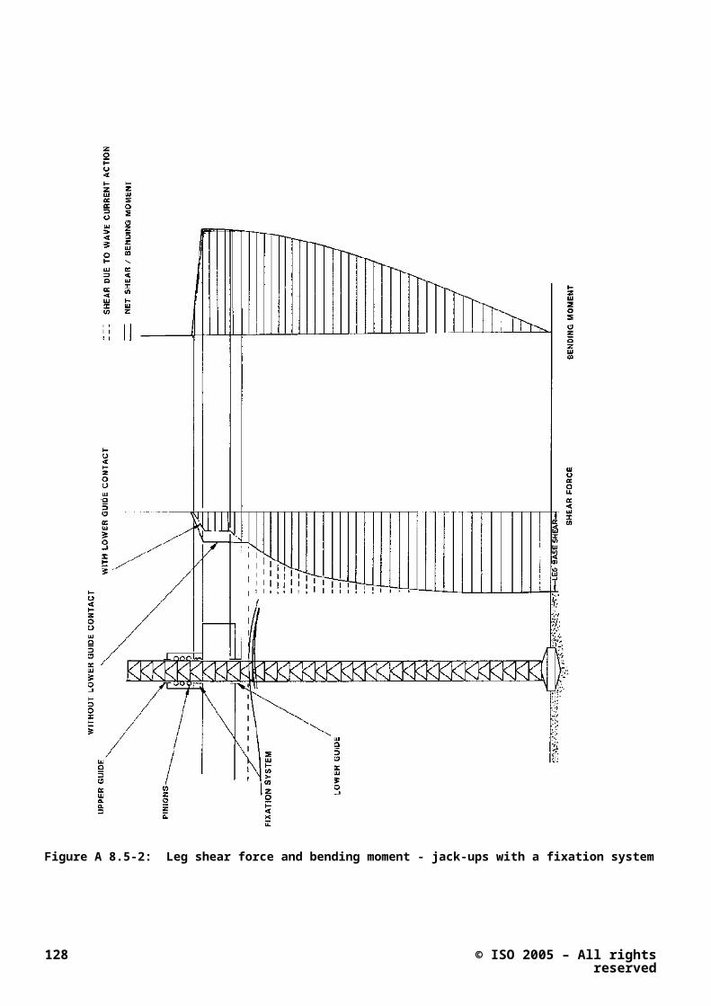
Figure A.9.2-1 Normalised inritial shear modulus as a function of Plasticity Index, Ip, for 11 different clays. Figure 10.2 from Anderson [55 – Needs to be changed]
The recommendations given above are intended for use in both site assessments for extreme loading and applications involving small strain beneath the spudcan. In the calculation of fixity for extreme loading, the moment stiffness based on the small strain G values will be degraded using the stiffness reduction formulae given in 6.3.4 of the Practice. In the case of small strain applications, such as in structural fatigue analysis, the stiffness reductions do not apply and it may be appropriate to adopt upper-bound values.
b) Selection of shear modulus, G, in sand
For sands the initial, small-strain shear modulus should be computed from:
=
where
= (dimensionless stiffness factor)
= atmospheric pressure
© ISO 2005 – All rights reserved 133
0 20 40 60 80 100
P lastic ity Index, Ip (% )
0
1000
2000
3000G
max
/ s u
DS
S
3
40
4
102540
2
2.8
2.8
1.9
1.0 < O C R <1.5O C R > 1.5. O C R ind icated a t data po int

= relative density (percent)
Vswl = seabed vertical reaction under still water conditions.
A.9.3.3.4.3 Extension of the yield surface for additional penetration
On seabeds of silica sands, conical spudcans which are not fully seated may show a plastic moment restraint due to further penetration. The effect may be taken into account for legs with QV/VLo > 0.
The moment capacity Mp associated with further penetration is estimated as the minimum of MPS and MPV, calculated as follows (Svanø [56 – Needs to be changed]):
MPS = 0.075 B VLo(DB/B)3
MPV = 0.15 B FVHM
in which B is the plan diameter of the effective contact area after preload, and D B is the plan diameter of the contact area when the spudcan is fully seated.
The combined capacity should be checked against the modified yield function:
For additional penetration of spudcans in clay, references C6 (to be changed) [49 – Needs to be changed] and [52 – Needs to be changed] provide work-hardening modifications to the yield surface equations. Updated stiffnesses are determined through plasticity principles.
53 Noble Denton Europe & Oxford University (2005), "The Calibration of SNAME Spudcan Footing Equations with Field Data", Report No L19073/NDE/mjrh, Rev 3, dated ????? 2005.
54 Templeton J.S., Lewis D.R., Brekke J.N. (2003), "Spud Can Fixity in Clay, First Findings of a 2003 IADC Study", 9th City University Jack-up Platform Conference, London.
55 Andersen K.H. (2004), "Cyclic clay data for foundation design of structures subjected to wave loading", Invited lecture, International Conf. on Cyclic Behaviour of Soils and Liquefaction Phenomena, CBS04, Bochum, Germany. Proc. p. 371 – 387.
56 Svanø G. (1996), "Foundation Fixity Study for Jack-Up Unit", SINTEF report STF22 F96660, August 1996.
57 Murff, J. D., M. D. Prins, E. T. R. Dean, R. G. James, A. N. Schofield, "Jack-Up Rig Foundation Modeling", Proceedings, Offshore Technology Conference, Houston, Paper No. 6807, May 1992, pp. 35-46.
58 van Langen, H., P. C. Wong, E. T. R. Dean, “Formulation and Validation of a Theoretical Model for Jack-Up Foundation Load-Displacement Assessment”, Proceedings, 6th International Conference on the Jack-Up Platform – Design, Construction and Operation, London, 1997.
59 Wong, P. C., J. C. Chao, J. D. Murff, E. T. R. Dean, R. G. James, A. N. Schofield, Y. Tsukamoto, “Jack-Up Rig Foundation Modeling II”, Proceedings, Offshore Technology Conference, Houston, Paper No. 7303, May 1993, pp. 411-420.
A.9.3.3.4.4 Deep footingspudcan penetrations
For deep footingspudcan penetrations, typically experienced in soft clay conditions, the calculation of foundation fixity may be augmented with the inclusion of the lateral soil resistance on the leg members due to soil back-flow over the spudcan. This lateral soil resistance is effectively added to the rotational elastic stiffness of the spudcan (as determined in Section A.9.4.3.1), (Brekke [37]).
134 © ISO 2005 – All rights reserved

The lateral soil resistance may be modelled based on concepts proposed by Matlock [38] for lateral soil resistance of piles. The jack-up leg may be modelled as an equivalent pile for purposes of determining "p-y", or load-deflection curves.
The diameters of the individual members (i.e., leg chords and braces) give appropriate characteristic dimensions for determining the p-y curves. The p-y curve for each member is summed to form a p-y curve for the entire leg. Only one face of each leg should be assumed to be in contact with the soil and contribute to lateral resistance.
Given a set of p-y curves for the leg, the lateral force-deflection along the entire embedded leg section is thus determined. Typically, equivalent springs at each bay elevation are used to simplify the calculations.
For overconsolidated clays (OCR 4) susceptible subjected to cyclic degradation loading (OCR 4) the soil rotational stiffness, calculated from the static soil properties, may be multiplied by a factor of 1.25, Anderson [36].
A.9.3.3.4.5 Foundation Settlement
Settlements of the jack-up rig foundation have to be estimated and checked. If necessary, corrective actions have to be taken. The settlements due to bearing capacity failure during to preloading are not part of this Section (Refer Section 6.2). The settlements of installed spudcans can be assessed from a combination of:
elastic settlements
consolidation settlement
settlements due to cyclic loading
settlements due to hydraulic instability
The elastic settlements and consolidation settlements can be calculated using conventional analytical or numerical geotechnical models.
The elastic settlements occur instantaneous and can be calculated as function of the basic elastic soil properties ( and G), the applied load and the boundary conditions. The consolidation settlements of cohesive soils can be calculated using conventional models accounting for time effects.
Cyclic environmental loading or operational vibrations may induce further settlements. Special attention should be given to cyclic loading in silty sand or silt. The cyclic loading may also involve a soil strength reduction. This may induce settlements due to bearing failure.
© ISO 2005 – All rights reserved 135
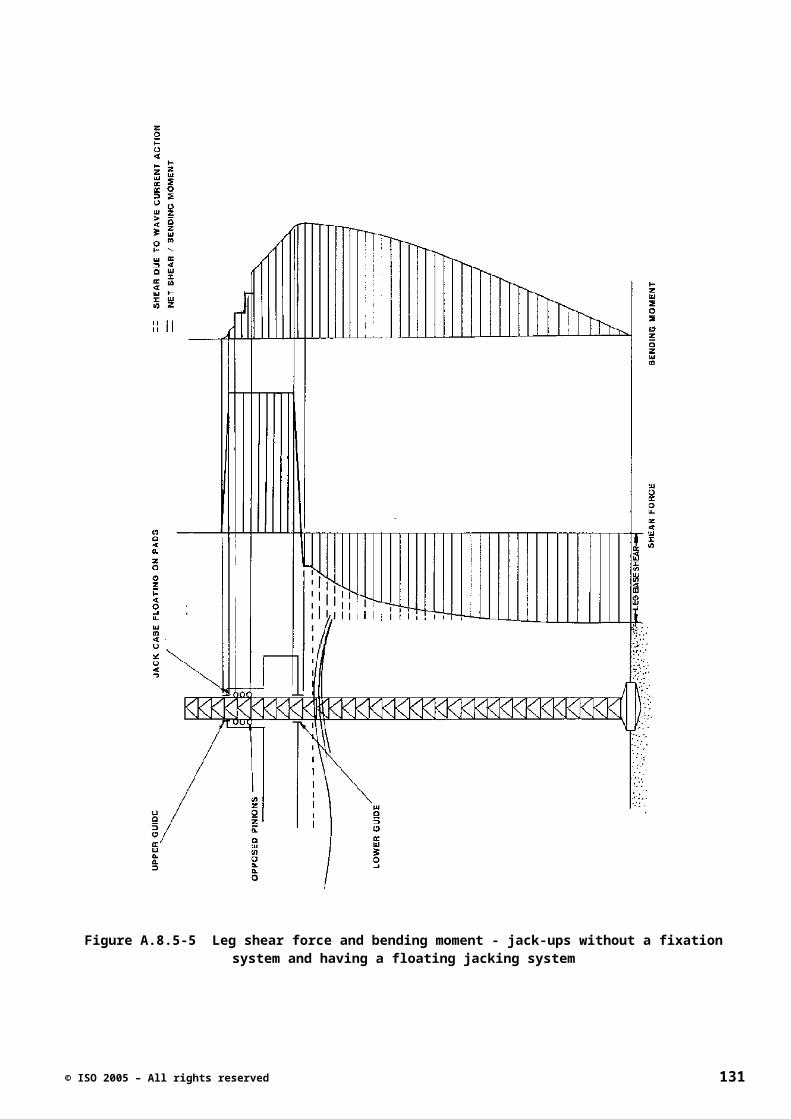
Figure A.9.3-6 — Procedure for assessment with foundation fixity
Seafloor instability due to scour or piping involves a decrease of the effective bearing capacity. This may induce settlements due to local bearing failure or due local increase of loading pressures.
136 © ISO 2005 – All rights reserved
Assume elastic spudcan response QM = K3θ, QV = K1δv, QH = K2δh,
Unit NOT acceptable
Performstructural assessment with
pinned case inertial loadset, See Sections 5,7 & 8.
Perform
foundation check at all spudcans (see 8.3.3)
OK Not OK
Not OK
OK
Unit acceptable
Run iterative structural analysis using current inertial loadset and de-grade foundation stiffness until spudcan loads fall within foundation yield surface. Section 6.3.4.2
Perform dynamic analysis accounting for fixity?
YesPerform simplified or
detailed dynamic analysis accounting for fixity?
No
Perform
foundation checks at all spudcans
(see 8.3.3)
Perform structural
assessments See Sections 5,7 & 8
OK
OK
Run dynamic analysis using linearised fixity and determine wave force transfer functions.
Run non-linear elasto-plastic dynamic time-domain analysis and determine DAF from a number of differing storm simulations. Use resulting DAF to determine new inertial loadset. (Section 6.3.4.1 Option 1)
Natural Period close to
cancellation point?
Select initial linearised fixity
Yes
Select revised linearised fixity &/or change hull mass.
No
Not OK
Perform Step 3
Not OK
Not OK
OKTry more complex method?
No
Yes
Unit NOT acceptable
Simplified
Detailed
Section 6.3.4.1 (Option 2)
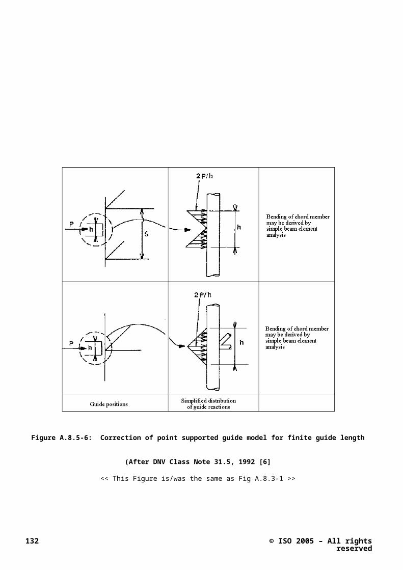
The settlements should be checked regularly. If necessary level adjustments should be made or protective measurements against scour development should be taken. (Section Clause 6.5.3)
A.9.3.4 Foundations equipped with skirts
Information on spudcans fitted with skirts can be found in the references listed below.
[1] Dean, et al. (1995), "Centrifuge Modelling of 3-Leg Jackups with Non-Skirted and Skirted Spuds on Partially Drained Sand", Proceedings Offshore Technology Conference, Houston, (OTC 7839).
[2] Eide, A., K. A. Tuen and M. Baerheim (1996), “The Yme Jack-up with Skirt Foundation”, Proceedings Offshore Technology Conference, Houston (OTC 8158).
[3] Svano and Tjelta (1993), "Skirted Spudcans - Extending Operational Depth and Improving Performance", 4th City University Jack-up Platform Conference, London.
A.9.4 Other considerations
A.9.4.1 Footprint considerations
Information on spudcan-footprint interaction can be found in the reference listed below:
[4] Stewart, D. P. and Finnie, I. M. S. (2001), “Spudcan- Footprint Interaction During Jack-up Workovers”, Proceedings, 11th International Offshore and Polar Engineering Conference, Stavanger, Vol. I, pp. 61-65.
A.9.4.2 Hard sloping strata at or below mudline
A hard sloping stratum can be created by a sand wave, sand bank, scour around a jacket or platform, buried geomorphic features such as channels, surface or buried footprints produced by previous jack-up unit emplacements, human-related seabed activity, or a combination of the above.
Eccentricity in the spudcan reaction can lead to emplacement and removal difficulties, particularly for slender brace/leg designs.
This eccentric loading can result in a significant leg bending moment in the region of the hull. Where the bending moment is reacted by the leg guides, a large shear force in the leg may result that could overstress the leg lattice members.
If a fixation system (rack chocks) is employed at the leg to hull interface, the bending moment present at the time when the fixation system is engaged will be locked into the leg. If the eccentricity of the spudcan reaction is subsequently exacerbated (e.g. by scouring around the spudcan), then the effective leg bending moment in the region of the hull may increase. When the fixation system is later disengaged, the moment in the leg will be redistributed in equilibrium with the present support conditions, which may result in overstressing of the leg members.
Where the jack-up unit is pre-stressed as a result of installation on such a seabed (e.g. by differential jacking on each chord of the leg), these installation stresses should be included in the overall site-specific assessment. Consideration may also be given to the potential benefit of seabed preparation prior to emplacement of the jack-up unit.
A.9.4.3 Leaning instability
No guidance offered
A.9.4.4 Leg extraction difficulties
Experience has shown that leg extraction difficulties are relevant but not limited to conditions such as:
© ISO 2005 – All rights reserved 137

Deeply penetrated spudcan in soft clay or loose silt
Skirted or caisson-type spudcan where uplift resistance is greater than the installation load.
Sites where soil exhibits strength gain with time.
The load required to extract the leg is a combination of several factors including the nature of the soils, the depth of penetration, the geometry of the footingspudcan and whether soil backflow has occurred behind the footingspudcan. Cassidy et al. [5] present the results from a limited number of centrifuge model tests performed on soft normally consolidated kaolin clay using a spudcan and caisson footing. The latter had a skirt depth to diameter ratio of 0.5. Immediate backflow occurred behind the footingspudcans in all tests and the caisson footing was sealed post installation prior to loading (i.e. the installation drainage valve was closed post-installation). A peak tensile load in the order of 0.5 times the maximum applied compressive installation load was observed for the spudcan footing. The caisson footing, when pushed into the soil to a depth of half a diameter, developed a peak tensile load ratio in the order of 0.6 times the maximum applied compressive load. However, depending upon the penetration depth and loading history, somewhat higher peak tensile load ratios were observed for the caisson foundation. For a caisson foundation that has not been penetrated into the ground (i.e. has not been loaded past its bearing capacity) the tensile capacity can be as much as the reverse undrained bearing capacity ([6] and [7]).
Craig [8] presented a very similar result for a single undrained centrifuge model experiment carried out using a 14m diameter prototype spudcan on a sand overlying clay foundation. In this case, a peak tensile load of 0.5 times the maximum compressive installation load was observed for a spudcan penetration to diameter ratio (D/B) of 1.0. Additional information is given in [9] and [10].
A jack-up unit pulls it legs from the seabed by lowering the hull into the water, which generates a buoyant uplift force and thereby induces tensile loading in the legs. In this manner a jack-up unit can typically apply a maximum tensile footingspudcan reaction of around 85% of the preload footingspudcan reaction, which generally ensures that legs with conventional spudcans are extracted without too much difficulty. However, where significant leg penetrations are attained, it is not uncommon for pulling of the legs to take several days, or in some cases much longer. Jetting on the underside and topside of the footingspudcans can be carried out to assist with leg extraction, though where leg extraction has been particularly difficult the following techniques have also been employed:
Alternating between compressive and tensile loading on the footingspudcan (i.e. working the legs up and down).
Use of a supplementary jetting system in the form of drill pipe and/or flexible tubing to jet on top of and around the sides of the footingspudcan.
Offloading as much variable load as possible to maximise hull buoyancy and hence the leg uplift load.
Excavation of the surface soils.
It should be noted that jetting and/or excavation of the surface soils can alter soil strength and the seabed topography, which could affect future emplacements of jack-up units at the same location.
References:
[5] Cassidy, M.J., Byrne, B.W. and Randolph, M.F. (2004). A comparison of the combined load behaviour of spudcan and caisson foundations on soft normally consolidated clay. Geotechnique 54(2).
[6] Byrne, B.W. and Cassidy, M.J. (2002). Investigating the response of offshore foundations in soft clay soils. Proc. OMAE’02 21st Int. Conf. On Offshore Mechanics and Artic Engineering, Oslo, Norway, Paper No OMAE2002-28057.
[7] Cassidy, M.J. and Byrne, B.W. (2001). Drum centrifuge model tests comparing the performance of spudcans and caissons in kaolin clay, University of Oxford Report OUEL 2248/01.
[8] Craig, W.H. (1998). Spudcan foundations: installation with deep penetration and subsequent removal. Geotechnical Engineering, Vol 131 No 3, pp146-151.
138 © ISO 2005 – All rights reserved

[9] Craig, W.H. and Chua, K. (1990). Extraction forces for offshore foundations under undrained loading. Journal of Geotechnical Engineering, Vol 116, No 5, pp 868-884.
[10]Craig, W.H., Cruickshank, M. and Fisher, R. (2002). Seabed breakout forces. Proc. Int. Conf. on Physical Modelling in Geotechnics 2002, Newfoundland, Canada. Balkema. pp 283-287.
A.9.4.5 Liquefaction and cyclic mobility
No guidance offered
A.9.4.6 Seafloor instability
No guidance offered
A.9.4.7 Scour
0.001
0.01
0.1
1
10
0.001 0.01 0.1 1 10 100 1000
Particle Size [mm]
Mea
n Fl
ow V
eloc
ity [m
/s]
CLA
Y Fine Medium Coarse Fine Medium Coarse Fine Medium Coarse
SILT SAND GRAVELBOULDERS
SedimentationTransport
Erosion
After McDowell & O'Connor (1977)
References
[11]Sweeney, M., Webb, R.M., Wilkinson, R.H. (1988): Scour around jackup rig footings, Proceedings of the 20th Offshore Technology Conference, Paper No. 5764, Houston, Texas, USA
[12]Whitehouse, R.J.S. (1998): Scour at marine structures, Thomas Telford Publications, London, UK
[13]Rudolph, D., Arnout C., Bos, K.J., Rietema, K.,. (2005): Scour around spudcans – analysis of field measurements, The Fifteenth International Offshore and Polar Engineering (ISOPE) Conference Korea, June , 2005.
© ISO 2005 – All rights reserved 139

A.9.4.8 Shallow gas
No guidance offered
A.9.4.9 Spudcan-pile interaction
No guidance offered (Put reference here for the Siciliano, et al. 1991)
A.9.5 Analysis of single (mat) foundations
No guidance offered
<< Symbols for section A9 now located in A.4.9 >>
140 © ISO 2005 – All rights reserved

A.10 Structural response
A.10.1 ScopeApplicability
No guidance offered
A.10.2 General considerations
Two aspects of the response are to be distinguished and assessed separately. These are:
a) The extreme response - The maximum calculated response to the design environment occurring at a particular instant in time. For typical jack-up assessment, the time-varying nature of the wave loading will amplify the quasi-static responses and must be considered. The extreme responses required forwhich must be assessedment are typically include the internal forces and moments offorces in the leg members, overturning moments of the jack-up, horizontal deflections of the hull of the joints, reactions and displacements at the spudcans, and loads in the pinionsholding system, and internal loads in the hull. The extreme responses should be obtained using appropriate combinations of fixed loads, variablefunctional loads, and wave/current and windenvironmental or seismic loads, and dynamic, second order and leg inclination effects with the load factors required by the acceptance criteria in<< wherever P10 puts them >>in Section 8. Load application is described in A.8.8. Section 5.7. Section 5.1 Clause 5.4.3 requires that the analysis is to be carried out for a range of environmental headings with respect to the jack-up such that the most onerous loading(s) for each major type of element in the structural system is(are) determined.
b) Fatigue - The cumulative effect of stress/strain cycling, which is used to estimate the fatigue lives of steel components (see Section 7.4). Clause 10 is specifically aimed at short-term operations where fatigue is typically not a consideration. However, fatigue response may can be important for long-term applications of a jack-up unit and the reader is referred to Clause 11.
A.10.3 Types of analyses and associated methods
The extreme response can be assessed determined either by a quasi-static analysis procedure including an inertial loadset or by a more detailed (random) dynamic analysis procedure. Figure A.10-1 shows the procedures for using these two approaches to determine the extreme response.
The quasi-static analysis procedure including an inertial loadset uses the deterministic method to calculate the extreme response. see Clause A.10.5.2). describes how to use the deterministic, quasi-static analysis with inertial load set for determining the extreme response for assessment.
The detailed (random) dynamic analysis procedure uses the stochastic method to predict the extreme response. (see Clause A.10.5.3). describes how to use the stochastic, random dynamic analysis for determining the extreme response for assessment.
Figure A.10-1 shows the procedures for using these two approaches to determine the extreme response.
© ISO 2005 – All rights reserved 141

Figure A.410-1 — Recommended approach to determine extreme responses (MJD to revise )
142 © ISO 2005 – All rights reserved
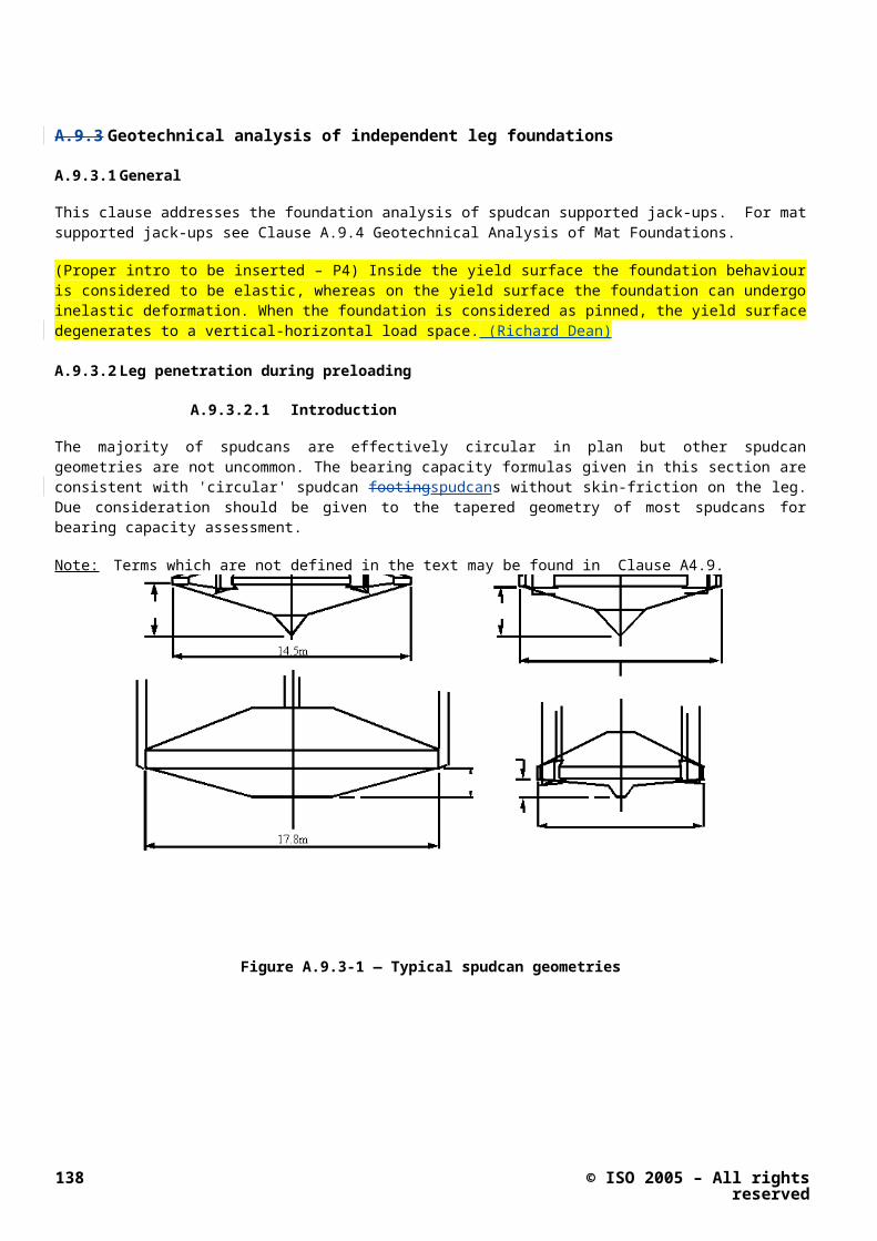
A.10.4 Generic factors
A.10.4.1 General
The magnitude of the extreme response may be calculated either by a quasi-static analysis procedure including an inertial loadset or by a more detailed (random) dynamic analysis procedure. will be affected by the parameters used in the analysis.
The magnitude of the quasi-static response is controlled by the structural stiffness of the jack-up and the magnitudes of the fixed loads, variablefunctional loads and environmental loads applied on the jack-up. Section 5 A.8 identifies the factors that affect the structural stiffness of the jack-up and Section 5.6A.8.x discusses the structural stiffness modeling at various levels of complexity. Section 4Clause 7 identifies the factors that affect the hydrodynamic and wind forces.
The magnitude of the dynamic response is primarily influenced by the amount of wave energyenvironmental excitation at or near the natural period of the jack-up and is therefore affected by the following two characteristics:
a) The dynamic characteristics (natural periods) of the structural system (natural periods) formed by the jack-up on its foundation, and
b) The characteristics of the wave-currentenvironmental excitation. << Higher order Harmonics ? >>
The following sections discuss the factors that affect these two characteristics.
A.10.4.2 Natural periods and affecting factors
A.10.4.2.1 General
The natural period of the jack-up on its foundation in the fundamental (or first) mode of vibration is an important indicator of the degree of dynamic response to be expected. The first and second vibrational modes are nearly always the surge and sway modes. The natural periods of these vibrational modes are usually close together; which of the two is the higher depends on which direction is less stiff. Where the natural or wave period varies with environmental heading, care should be taken that the periods used is are applicable to the environmental direction being considered in the analysis. The third vibrational mode is normally a torsional mode, the three-dimensional effects of which may can be important, in particular for environmental attack directionsheadings where the legs and hence wave loads are not symmetric about the direction of wave propagation.
<< wave cancellation discussion moved to TR by PLTan and brought back by Nov 2005 Review panel as below - needing work. Action confirmed by March 2006 Review panel, >><< mjrh: Where have the deleted paras above been placed ? >>
The natural period is dictated by the characteristics of the structural system, which are governed by the overall (global) structural stiffness, the mass and mass distribution and the damping.
The undamped natural period is determined from the following equation:
Tn = 2
where;
Tn = highest (or first mode) natural period.
Me = effective system mass;
Ke = effective system stiffness.
Due to uncertainty in parameters affecting the natural period, the calculated natural period(s) will also be uncertain. The natural period(s) used in the dynamic analysis should be selected such that a realistic but conservative value
© ISO 2005 – All rights reserved 143

of the dynamic response is obtained for the particular application envisaged. Care should be taken to ensure that the maximum dynamic amplification is not selected as coincident with a cancellation period causing minimum environmental loading. The potential for increased response due to shortcrested waves should be considered (see Clause xxx). << Put the figures presently in Annex C here >> For further details refer to Annex << or TR >> xxxx.
<< Re-write with better explanation and methods to avoiding the problem. >>
A.10.4.2.2 Stiffness
The jack-up on its foundation represents a multi degree-of-freedom system. If available, a finite element structural model, containing the mass and stiffness properties, of the jack-up should be used to obtain the various natural periods and mode shapes.
Structural modelingmodelling at various levels of complexity is discussed in A.8 Section 5.6 and should include stiffness contributions from the bending, shear deformation and axial straining of the legs, the leg to hull connections, the hull and the spudcan-foundation interface (if applicable) considering the following effects:
1) bending of the legs, leg-soil and leg-hull rotational stiffness.;
2) shear deformation of the legs;.
3) axial deformation of the legs;.
4) hull bending deformation;.
5) horizontal vertical and rotationalsoil and leg-hull connection stiffness;.
6) horizontal, vertical and rotational foundation soil and leg-hull connection stiffness;.
7) second order P- or Euler stiffness reductionamplification.
The model may contain a number of nonlinear elements, notably the leg to hull connections and the spudcan-foundation interfaces.
If desired such a capability (a finite element structural model containing the mass and stiffness properties of the jack-up) is not available, due to the fact that the mass of the hull dominates the mass distribution, the system stiffness for the fundamental modesglobal dynamic behavior of the jack-up may in some cases be determined from an idealized single degree-of-freedom system and thus the fundamental mode period may be determined from an idealized single degree-of-freedom systembe estimated as described in Annex C << P3 suggested TR >>.
<< The above deleted section has been moved to the Technical Report (TR) - or Annex C >>
A.10.4.2.3 Mass
No guidance offered – See Clauses 8.8 and A.8.8 for guidance.
A.10.4.2.4 Variability in natural period
?? – May add text later
A.10.4.3 Damping
System damping contributors include foundation, hydrodynamic and structural damping. Non-linear behaviour of the foundation and jacking system also contribute to system damping. The degree to which each of these contributes to damping will depend on the type of analyses and the level of system response. Damping may be accounted for explicitly or implicitly:
Explicit damping is input to the analysis as a percentage of critical damping e,g 3% hydrodynamic;
144 © ISO 2005 – All rights reserved

Implicit damping arises as a function of the analytical response and modelling e.g. fluid-structure relative velocity for hydrodynamic damping and hysteresis for foundation damping.
Where the model relies on explicitly defined damping, then the total system damping shall not exceed 7% without credible, applicable justification. Lower values may be appropriate for fatigue analyses and smaller seastates. Care should be taken with the explicit and implicit representation of damping in the analyses e.g. relative velocity hydrodynamic damping and soil hysteretic damping. Table A.10.4-1 summarizes appropriate typical upper bound percentages of critical damping for the various damping sources that should be summed to providecomprise the total explicitly defined damping.
Table A.10.4-1 — Recommended explicit damping from various sources
Damping source Global damping not to exceed (% of critical damping)
Structure, holding system, etc. 2%
Foundation 2% or 0%(1)
Hydrodynamic 3% or 0%(2)
NOTES 1. Where a non-linear foundation model is adopted the hysteresis foundation damping will be accounted for directly and should not therefore be included in the global damping.
2. In cases where the relative velocity formulation may be used ( = 1 in Section 4.3.2) the hydrodynamic damping will be accounted for directly and should not therefore be included in the global damping.
<< This will need a rewrite when we include the Templeton (2006) stiffness and damping >>
Table A.10.4-1 — Recommended damping from various sources
A.10.4.4 SoilsFoundations
Typically the initial linearized rotational stiffness for the dynamic analysis may be taken as 80% of the value determined from the formulation in <<Clause 9??? SNAME 6.3.4.3>>
<<< move to cancellation discussion in TR; This stiffness may need to be further adjusted to avoid wave force cancellation. The adjusted value may lie anywhere between 0% and 100% of the value from <<Clause 9??? SNAME 6.3.4.3>>>No guidance offered.
A.10.4.5 Directionality and spreading<<< this one goes to Panel ½>>>
The effects of directionality and wave spreading may be considered in any random dynamic analysis. It is recommended that a comparison be made between the Base Shear Transfer Function (BSTF) for the chosen 2-D (long crested/unspread) analysis direction and the 3-D (short crested/spread) BSTF to determine whether the selected direction is unconservative. Optimally the direction of the 2-D seastate should be chosen to obtain a match with the 3-D BSTF for the entire wave spectrum. If this is not possible the match between the spread and unspread BSTFs should be good at the natural period.
A 3-D BSTF, H3D, can be generated from a set of 2-D BSTFs, H2D, by the following expression:
H3D() =
where:
= Wave excitation frequency
= Angle between 2-D BSTF and dominant direction of 3-D BSTF
n = Power constant of spreading function
© ISO 2005 – All rights reserved 145

2.0 for fatigue analysis
4.0 for extreme analysis
A simple approximation to the incorporation of wave spreading into inertial load calculations is to perform a 2-D analysis with the wave approach angle which is between the two approach angles which give the maximum and minimum forces at the cancellation and reinforcement points (see Figure C7.1 in the Commentary).
A.10.4.6 Storm Excitation
Currents change slowly compared with the natural periods at which jack-ups may oscillate and may hence be considered to be a steady phenomenon. Variations in wind velocity cover a wide range of periods, but the main wind energy is associated with periods whichperiods that are considerably longer than the natural periods of jack-up oscillations. Therefore, in connection with jack-ups, the wind may generally be represented as a steady flow of air. The periods of waves typically lie between some 2-3 sec and some 20 sec. Since typical jack-up natural periods fall within this range, the primary source of dynamic excitation is from waves.
Sea waves are generally not regular but random in nature unless swell is predominant. This has important implications whichimplications that should be considered for both the dynamic excitation and the resulting dynamic response.
A.10.5 Storm analysis
A.10.5.1 General
No guidance offered
A.10.5.2 Deterministic storm analysis
The quasi-static analysis shall be carried out in accordance with all relevant requirements of Sections 3 to 6. The maximum wave loading is determined by 'stepping' the maximum wave through the structure. The maximum wave is defined in Section 3.5.1.2 and the methodology for calculating the wave loading is described in Section 4.3. Load cases and combinations are discussed in Section 7.1.7.A.10.5.4x.x.
The inertial loads are determined from a dynamic amplification factor (DAF). Methods for determining the dynamic amplification factors (DAFS or DAFR) and subsequently the inertial loadset are given in Section A.10.5.2.1.
<< ADD A FIGURE RE AMPLITUDES AND DEFINE DAFS and DAFR etc. >>
The spudcan-foundation interface should normallycan be modeledmodelled as a pin joint. The inclusion of a degree of fixity is to be justified on a case by case basis. If foundation fixity is included it shall should generally be represented by a combination of horizontal, vertical and rotational springs (which may be coupled) at the spudcan , and not rather than by a rotational spring alone. The inclusion of foundation fixity shall be in accordance with Clause 9. (See also Sections 5.3, 6.3.4 and 7.3.5.2).
A.10.5.2.1 Dynamic amplification factors (DAF) and inertial loadsets
A.10.5.2.1.1 General
When using the deterministic analysis for determining calculating the extreme response, the dynamic actionresponse is represented by an equivalent point load applied at the hull. center of gravity. The inertial loadset may be derived from the simple approach described in Section A.10.5.2.1.21 or from the more complex methods discussed in Section A.10.5.2.1.32.
146 © ISO 2005 – All rights reserved

A.10.5.2.1.2 The classical SDOF analogy
This representation assumes that the jack-up on its foundation may be modeledmodelled as an equivalent mass-spring-damper mechanism. The (highest) natural period of the vibrational modes may be determined as described in Section A.10.4.12. The torsional mode and corresponding three-dimensional effects cannot be included in this representation.
The single degree-of-freedom (SDOF) method is fundamentally empirical because (1) the wave-current loading does not occur at the mass centrehull and (2) the loading is non-periodic (random) and non-linear. It should also be noted that all global and detailed response parameters are not equally amplified. See TR << Annex C >> for guidance on using the single degree-of-freedom (SDOF) for deriving the DAF and inertia loadset.
The method described below will generally lead to a reasonable approximation of the jack-up's real behavior and has been calibrated against more rigorous methods. The following cautions are noted when using the SDOF method:
8) If the ratio of the jack-up natural period to the wave excitation period, , is less than 0.5 and the current is 'relatively small' the SDOF method should give reasonably accurate results when compared to a more rigorous analysis.
9) If is greater than 0.5, the relative position of the jack-up natural period within the base shear transfer function should be checked. If the natural period falls near a wave force peak, then the SDOF method can be unconservative because it ignores forcing at other than the full wave excitation period. Note that a range of natural periods should be considered to account for a reasonable range of foundation fixity (see A.10.x.x).
10) The SDOF method can be unconservative for cases with relatively high currents. If the results of the assessment are close to the acceptance criteria further detailed analysis is recommended.
The ratio of the single amplitudes (and not the absolute values or ranges) of the dynamic to the quasi-static response as a function of frequency () or period (T) of steady state, periodic and sinusoidal excitation is calculated as the classical dynamic amplification factor (DAFS):
DAFS =
where;
=
=
= Damping ratio or fraction of critical damping
= (% Critical Damping)/100, 0.07.
T = 0.9Tp.
Tp = most probable peak wave period.
Tn = the jack-up natural period as derived in 7.3.5.
© ISO 2005 – All rights reserved 147

The damping parameter in this model represents the total of all damping contributions (structural, hydrodynamic and soil damping). For the evaluation of extreme response using the SDOF method a value not exceeding 0.07 is recommended. << Will need revision when Templeton (2006) is introduced >>
The calculated DAFS from the SDOF method is used to estimate an inertial load which represents the contribution of dynamics over and above the quasi-static response in accordance with Figure 7.1. This inertial load should be determined as follows and applied at the hull in the down-wind direction:
Fin = (DAFS - 1) BSAmplitude
where;
Fin = Magnitude of the inertial loadset for use in conjunction with the SDOF method.
BSAmplitude = Single Amplitude of quasi-static Base Shear over one wave cycle.
= (BS(Q - S)Max - BS(Q - S)Min)/2
BS(Q - S)Max = Maximum quasi-static wave/current Base Shear.
BS(Q - S)Min = Minimum quasi-static wave/current Base Shear.
Note: The above equation is part of a calibrated procedure and should not be altered. A more general inertial loadset procedure, using the results from random analysis, is described in Section 7.3.6.3.
<< The above deleted section has been moved to the Technical Report (TR) - or Annex C >>
A.10.5.2.1.3 Inertial loadset based on random dynamic analysis
(Note PLT to work on rewrite of this section)
The inertial loadset can also be derived from the DAF calculated based on from a random frequency or time domain analysis for random-wave excitation according to the recommendations of the Stochastic Storm Analysis in Section 7.3.7 (A.10.5.3). The DAFR is to be the ratio of the Most Probable Maximum Extreme (MPME) of the dynamic response to the MPME of the static response (MPMEdyn/MPMEstatic). The MPME is defined in Table 7.3 as the extreme with a 63% chance of exceedence (typically this is the mode or highest point on the probability density function (PDF)). This is approximately equivalent to the 1/1000 highest peak level in a 3-hour storm.
The inertial loadset should be such that it increases the responses of the deterministic quasi-static analysis by the same ratios as those determined between the random quasi-static (zero mass) analysis and the random dynamic analysis. In such cases the structural model (used for dynamic analysis) may be simplified and does not need to contain all the structural details, but will nevertheless be a multi degree-of-freedom model. An equivalent single point load applied at the hull centre of gravity to match the inertial moment effect can be used as an inertial loadset. << WE SHOULD TRY TO MATCH DYNAMIC BS & OTM - PROVIDE GUIDANCE ON THE WAYS THIS CAN BE ACHIEVED >>
A.10.5.3 Stochastic storm analysis
As an alternative to the deterministic Storm Analysis, the extreme response can also be predicted by a stochastic method of analysis. As the dynamic amplification of the structural response must be taken into account in the extreme response and the waves are random in nature, the stochastic method of analysis for predicting the extreme response must be based on the results of a random wave dynamic analysis.
The waves can be modelled as a linear random superposition model whichmodel that is fully described by the wave spectrum (see Section 3.5.3). The random wave dynamic analysis can be carried out in thea time domain or frequency domain. Table 7.2 identifies the most important factors constraints associated with each of these two types of methods for random wave dynamic analysis.
148 © ISO 2005 – All rights reserved

<<shouldn’t this be defined by the we need met-ocean partial factors (? sqrt(1.15) ?) that allow us to metocean/assessment panels such that achieve the same levels of reliability are assuredwith a load factor of 1.0 and the regular resistance factors. The solution may not be as simple as it appears; wave asymmetry, spreading, MPM's for non-linear systems provide added complications to achieving the desired degree of comparability with the more accurate method (less modelling uncertainty) requiring less conservatism. >>.
A.10.5.3.1 Random Wave Dynamic Analysis Method
Frequency domain methods require the linearization of the wave-current drag loading. It is recommended that the statistical (or least squares) linearization procedure formulated by Borgman is adopted [L.E. Borgman, ‘Ocean Wave Simulation for Engineering Design’, Civil Engineering in the Oceans, ASCE conference, San Francisco, September 1967]; other forms of linearization may not adequately handle the current velocity, wave induced particle velocity and the structures velocity (if a relative velocity formulation is used). Table 7.2 makes some additional recommendations regarding the generation of the random seastate.<< reference should be moved to the bibliography >> GET RVA’s input on this.
Time domain simulations require that a suitable random seastate is generatedion of the random seastate, that the validity of the generated seastate is checked, and that the time-step for the solution of the equations of motion is sufficiently small. It is also necessary to ensure that the duration of the simulation(s) is sufficient for the method being used to determine the MPME. Specific recommendations are given in Tables 7.2 and 7.3
Table A.10.5-1 - Recommendations for application of random wave dynamic analysis methods
Method Recommendations
FrequencyDomain
Consider linearization assumptions with respect to:
- wave-current loading (quadratic dependence on particle velocity and finite wave height).
- structural non-linearity.
Generate random sea from at least 200 components and use divisions of equal frequency.Note: fewer frequency components may be used provided that the divisions are shown to be sufficiently small around the wave period, the natural period & periods associated with reinforcement and cancellation.
Time Domain
Generate random sea from at least 200 components and use divisions of generally equal energy. It is recommended that smaller energy divisions are used in the high frequency portion of the spectrum, which will generally contain the reinforcement and cancellation frequencies. Each wavelet should be taken to disperse with its own linear dispersion relationship [12]
Check validity of wave simulation: correct mean wave elevation
standard deviation = (Hs /4) ± 1%
- -0.03 < skewness < 0.03
2.9 < kurtosis < 3.1
Max crest elevation = (Hs/4){2ln(N)} -5% to +7.5%where N is the number of cycles in the time series being qualified, N Duration / Tz
Integration time-step less than the smaller of:
Tz/20 or T /20
© ISO 2005 – All rights reserved 149

where;
Tz = the zero-upcrossing period of the wave spectrum
Tn = the jack-up natural period
(unless it can be shown that a larger time-step leads to no significant change in results)
Avoid transients in 'run-in' (100 secs).
Ensure simulation length OK for method chosen to determine the Most Probable Maximum Extreme (MPME) response(s).
Note: The MPME is defined in Table 7.3
Table 7.2 - Recommendations for application of random wave dynamic analysis methods
A.10.5.3.2 Methods for Determining the MPME
When using the stochastic method to predict the extreme response from the results of a random wave dynamic analysis, it should be noted that the extreme response should be the required most probable maximum (MPM) response, which is defined in Table 7.3 as the mode value (or highest point on the PDF with a 63% chance of exceedance). This corresponds to a 1/1000 probability level in a 3-hour storm.
The waves may be modeledmodelled as a linear random superposition model which is fully described by the wave spectrum (see Section 3.5.3). The statistics of the underlying random process are gaussian Gaussian and fully known theoretically. An empirical modification around the free surface may be needed to account for free surface effects. This, together with the fact that drag forces are a nonlinear (squared) transformation of wave kinematics, makes the hydrodynamic force excitation always nonlinear. As a result, the random excitation is non-gaussianGaussian. The statistics of such a process are generally not known theoretically, but the extremes are generally larger than the extremes of a corresponding gaussian Gaussian random process. For a detailed investigation of the dynamic behaviorbehaviour of a jack-up the non-gaussian Gaussian effects must be included.
Four Three methods for obtaining the Most Probable Maximum Extreme (MPME) of this non-gaussianGaussian response are recommended below. Table 7.3A.10.x.x identifies the most important factors associated with each approach to determining the extreme responses.
It should be noted that the simpler modelingmodelling approaches will not lead directly to the MPME of all quantities of interest. For example, SDOF based models will provide directly only the MPME hull displacement; simpler multi-degree-of-freedom models may can provide the MPME of total leg loads, but will not lead directly to loads in individual members of a truss-leg.
It should also be noted that the application of the load factors required in section 8 may can be difficult for using the stochastic method to predict the extreme response. << ? we will now use partial metocean factors ?? >>
As a means of circumventing this difficulty, the random wave dynamic analysis may be used solely to determine the inertial loadset which represents the contribution of dynamics over and above the quasi-static response (see Figure C7.B.1 << OK, but will need major updating >>).
The four three recommended methods for determining the MPME are as follows
Use of drag-inertia parameter (or equivalent) determined from mean and standard deviation of a frequency or time-domain analysis.
Fit Weibull distribution to results of a number of time-domain simulations to determine responses at required probability level and average the results.
Fit Gumbel distribution to histogram of peak responses from a number of time-domain simulations to determine responses at required probability level.
Apply Winterstein's Hermite polynomial method to the results of time domain simulation(s).
150 © ISO 2005 – All rights reserved

Table A.10.5-2 - Recommendations for determining MPME (see Commentary)
Method Recommendations
General Define the Most Probable Maximum Extreme (MPME) as the extreme with a 63% chance of exceedance (typically this is the mode or highest point on the probability density function (PDF)).This is approximately equivalent to the 1/1000 highest peak level in a 3-hour storm.
Frequency Domain
Use mean & standard deviation to determine drag-inertia parameter and use Figure C7.B.6 in Commentary Section C7.B.2.1.
Time Domain Use mean & standard deviation to determine drag-inertia parameter and use Figure C7.B.5 or Figure C7.B.6 in Commentary Section C7.B.2.1. Simulation time of at least 60 minutes usually required to obtain stable standard deviation.
or
Fit Weibull distribution to distribution, for 3-hour probability level. Take results as average of MPME's from 5 simulations. Each input wave simulation to be of
sufficient length for recommendations of Table 7.2 to be met (usually at least 60 minutes). See Commentary C7.B.2.3.
or
Use multiple 3-hour simulations and use Gumbel distribution on the extreme from each simulation. Sufficient simulations (usually at least 10) are required to obtain stable MPME of responses. See Commentary C7.B.2.4.
or
Use Winterstein's Hermite polynomial model, with improvements by Jensen if Kurtosis kurtosis > 5. Simulation of sufficient duration to provide stable skewness and kurtosis of responses (normally in excess of 180 several hoursminutes). See Commentary Section C7.B.2.5.
Table 7.3 - Recommendations for determining MPME (see Commentary)
See TR << Annex C >> for additional guidance.
<< The deleted section above has been moved to the Technical Report (TR) - or Annex C >>
A.10.5.4 Leg Inclination
The effects of initial leg inclination should be considered. Leg inclination may can occur due to leg-hull clearances and the hull inclination permitted by the operating manual. Thus the total horizontal offset due to leg inclination, OT, may can be determined as:
OT = O1 + O2
where;
OT = Total horizontal offset of leg base with respect to hull.
O1 = Offset due to leg-hull clearances.
O2 = Offset due to maximum hull inclination permitted by the operating manual.
If detailed information is not available, OT should be taken as 0.5% of the leg length below the lower guide.
The effects of leg inclination need be accounted for only in structural strength checks. This will normally be accomplished by increasing the effective moment in the leg at the lower guide by an amount equal to the offset O T
© ISO 2005 – All rights reserved 151

times the factored vertical reaction at the leg base due to permanent, variable, environmental, inertial and P- loads.
A.10.5.5 Limit state checks
The extreme responses for assessment should be determined using appropriate combinations of gravity permanent loads, variable loads, wave/current loads and wind loads as required by the acceptance criteria in Section 8Clause 13. Load application is described in Section 5.7. Section 5.1 requires that the analysis is carried out for a range of environmental headings with respect to the jack-up such that the most onerous loading(s) for each major type of element in the structural system is(are) determined. The checks cover:
Table A.10.5-3 — xxxx
Load Component
Limit State Check SectionClause
Response Parameters(s)1 L note 2
D min max E Dn
Strength of elements 8.112 Element load vectors3 Y Y4 Y Y Y
Overturning8.213
Overturning moment 5 5 Y Y
Stability Stabilizing moment Y5 Y5
Foundation capacity: 8.39
- preload 8.3.19.xx Vertical leg reaction Y Y Y Y
- sliding 8.3.19.xx Vertical & Horizontal leg reactions Y Y Y Y
- bearing 8.3.2/39.xx
Vertical, Horizontal (& moment) leg reactions Y Y6 Y6 Y Y
- displacement 8.3.49.xx Leg footingSpudcan displacements and reactions Y Y6 Y6 Y Y
Horizontal deflection 8.413.x Hull displacement. Y Y6 Y6 Y Y
Holding system loads 8.513.y Holding system loads vectors Y Y4 Y6 Y Y
where D, L, E and Dn are defined in the glossary at the end of section 7.
NOTES
1. In all instances the responses are evaluated including the effects of deformation under dead functional loads (hull sag) and large displacement (P-) effects.
2. Placed at most onerous center of gravity position.
3. The effects of leg offset to be added after global response analysis (see Section 5.4).
4. Consider minimum live (variable) load if this is more onerous.
5. Must be included in response calculation so P- effects are included.
6. Worst case combination required.
152 © ISO 2005 – All rights reserved

A.10.6 Fatigue
No guidance is offered.
A.10.7 Earthquake
A.10.7.1 General
If operating close to an active fault, it may can be necessary to consider near source ground motions. These have been found to be considerably in excess of the normal design values with large ground motions at relatively long periods. << This may belong on A.7 >>
A.10.7.2 Soils
No guidance is offered.
A.10.8 Accidental situations
No guidance is offered.
<< ?? >>
A.10.9 Alternative Analysis Methods
A.10.9.1 Ultimate strength analysis
No guidance offered.
A.10.9.2 Types of analysis
Care should be taken when using 19902 in modelling non-linear behaviour of chords and holding system of a jack-up structure.
<< ?? >>
© ISO 2005 – All rights reserved 153

A.11 Long term applications
A.11.1 Scope
No guidance offered.
A.11.2 Assessment data
A.11.2.1 Jack-up data << latest P11 draft has Unit in place of Jack-up - it seems they started from an out-dated draft >>
For the assessment of the jack jack-up a list of relevant modifications shall include information about weights, wind areas and appurtenances added or removed that affect applied actions and structural integrity.
This can include:
Increased weight and wind area from such items as production modules, risers, flare towers, accommodation blocks, and conductors.
Increased wave and current actions due to risers, conductors or other structures exposed to waves.
A.11.2.2 Metocean data
Joint probability and/or directional metocean data may be more relevant for the long term application. The data required for a fatigue analysis shall include long term wave distribution and wave scatter data, refer to A.6.4.2.9.
Refer to xx.x for the partial action factor to be used for extreme storm analysis. For fatigue analysis the partial action factor may be reduced to unity when using S-N curves at -2SD.
A.11.2.3 Geotechnical data
Effects of seabed scour, differential settlement, consolidation settlement, reservoir subsidence and sand waves etc. may be more significant for long term application at a site. For this reason site specific geotechnical data shall include information necessary to evaluate these phenomena.
A.11.2.4 Other data
In addition to the above further data associated with long term use may be needed such as the possible affect on geotechnical properties due to top-hole construction activities..
A.11.3 Special requirements
A.11.3.1 Fatigue Assessment
In order to assess existing fatigue damage, specific information relevant to prior installations is advantageous. The availability of the information will depend on the information collected and retained by the rig owner over the life of the jack-up. The quality of the database will affect the historical results. The historical data may have a large variability requiring the assessor to make assumptions in the historical fatigue assessment. The assessment may include detailed fatigue analysis of the historical data and/or evaluation of inspection records
The number of prior site installations with similar parameters should be assessed in the context of the proposed long term site. Parameters identified as important in addressing the historical aspects of jack-up fatigue are as follows:
11) Site location including region (e.g. Gulf of Mexico, North Sea, Eastern Canada etc);
154 © ISO 2005 – All rights reserved

12) Hull Elevation;
13) Water Depth;
14) Penetration; and
15) Soil Type and Characteristics.
The required margin of safety of a structural detail shall depend on its accessibility for inspection and the availability of one or more alternative load paths (redundancy) after failure of the detail investigated.
The assessment shall take into account the fatigue history of critical details prior to installation on the planned site and focus on details of members that are essential for the overall structural integrity of the jack up. Areas that are susceptible may include:
The leg members and joints in the vicinity of the upper and lower guides for the operating leg/guide locations(s);
The leg-to-hull holding system;
The leg members and joints adjacent to the waterline;
The leg members and joints in the lower part of the leg near the spudcan; and
The spudcan to leg connection.
Other special considerations in the fatigue assessment are listed below:
Inclusion of detailed models to arrive at local stress levels:Areas in the structure with high stress levels may be identified using models developed for global analysis. For fatigue assessment it may be necessary to use more detailed models to identify the actual locations of high stress. The hotspot stress may be determined using fine mesh models (as defined in various codes) or by using appropriate SCF (Stress Concentration Factors) from literature.
Effect of foundation stiffness (seabed fixity)The stiffness of the foundations may normally be determined only within certain bounds. As a consequence, an upper and lower bound analysis may be required. Typically the fatigue assessment of the spudcan and lower part of the leg requires the use of upper bound stiffness while the fatigue assessment for the upper leg and the leg to hull interface requires lower bound stiffness. Furthermore the assessment may take into account that foundation stiffness varies according to loading on the spudcan. The stiffness will be higher at low spud can loadings and lower at high spud can loadings.
Inclusion of geometrical non-linear effects (Refer to Clause 8.7.6)
Inclusion of non-linear (Wave) loading:The structural response of a jack-up is such that pure linear techniques may not be adequate. Therefore the analysis tools should include the non-linear effects of the structure, wave-loading and dynamic response.
Inclusion of dynamic amplification (Refer to Clause 10)
Taking into account that some structural elements transfer load in compression contact only, i.e. such elements are loaded by half the load range only (leg guides, jacking and fixation systems).
A robust analysis method shall be used to determine the fatigue capacity. The method shall determine the response of the jack-up structure to various seastates representing the operational environment. << Review Panel Feb 06 : In light of debate with WG3 and SC7 regarding long-term application of jack-ups for production we need this clause to provide firm guidance acceptable to SC7. P11 should offer references to suitable methodology. See if clause 16 of 19902 can be used, perhaps with jack-up specific modifications. Otherwise reference Class Rules/Guidance ? >>
© ISO 2005 – All rights reserved 155

The jack-up configuration shall be considered in the operational phase. This configuration includes the levels of variable load, hull elevation and cantilever position.
Wave spreading and directionality effects are permitted to be included.
Foundation stiffnesses are generally assumed as linear in smaller seastates. A check of non-linearity is required to validate this assumption for higher seastates.
The required margin of safety of a structural detail shall depend on its accessibility for inspection and the availability of one or more alternative load paths (redundancy) after failure of the detail investigated. The acceptance criterion for fatigue capacity is as follows:
ff*SD + ED < 1.0 << why were we factoring history ?? is this a Norwegian thing >>
ff*(SD+ED)<1.0
Where:
SD = Fatigue damage during planned operations on site
ED = Existing fatigue damage prior to arriving at site
ff = fatigue factor, this factor is determined as follows:
Description No Access
Full access
No Redundancy/Major Consequence 3 2
Full Redundancy/Minor Consequence 2 1
Fatigue life enhancement methods such as weld profiling or weld toe grinding may be considered.
A.11.3.2 Weight control
An installation change procedure shall be prepared to track installation changes during the long term operation and the affect on the site assessment. This shall include wet weights were applicable. Due to the long term application, weight changes may be significant and these should be monitored to maintain the original assessment assumption.
The weight control plan shall be sufficient to satisfy the Classification Societies requirements in lieu of the periodic dead weight survey.
A.11.3.3 Corrosion protection
No guidance offered << added by MJRH >>
A.11.3.4 Marine Growth
Marine growth during the application period may be taken into account in the site assessment or monitored and removed.
A.11.3.5 Foundations
Consolidation of the soil through distribution of pore pressures over the long term operation may result in additional settlement. This consolidation settlement should be addressed in the assessment.
156 © ISO 2005 – All rights reserved

Where settlement has occurred, re-levelling of the rig may have consequences which should be considered in the assessment. In some conditions where scour may occur, scour protection may be required.
A.11.4 Survey requirements
A.11.4.1 Project specific inspection plan
The extent and types of inspections should be decided during the project-planning phase. A special survey shall be undertaken prior to going to site and in-service inspection program developed.
An inspection plan shall be prepared that specifies location and type of inspection. This should take into account the actual critically stressed and fatigue sensitive areas identified during the assessment. The plan shall also describe access to areas that are to be inspected.
Areas not accessible for inspection during operation shall be specially evaluated (see 11.3.1).
Areas that require special procedures for inspection such as underwater parts shall be inspected in accordance with an approved procedure giving due consideration to the most suitable and practical methods.
A.11.4.2 Special Survey
The jack-up shall comply with the special survey requirements of the Classification Society rules. This survey shall be performed prior to going to site.
A.11.4.3 In-service inspection program
The existing In-service Inspection Program normally required for Classification shall be modified and updated to reflect the requirements for the planned long term application defined in 11.4.1.
The results of the in-service inspections should be reviewed. If appropriate, the In-service Inspection Program should be modified to reflect this review. This information may be relevant for extending the jack-ups time on location beyond the original plan period.
A.11.4.4 Alternative In-service inspection program surveys
An alternative IIP may be derived using a probabilistic approach. The safety philosophy behind the alternative IIP shall be in accordance with the Classification Society's safety philosophy and the structural reliability level inherent in the Classification Society rules shall be maintained. The developed approach shall be documented.
When using a probabilistic approach it should be recognised that uncertainties are associated with prediction of the fatigue performance and the inspection techniques applied. Key uncertainties need to be accounted for in the probabilistic analysis.
© ISO 2005 – All rights reserved 157

A.12 Member checkingStructural Strength
A.12.1 Scope and overview
No Guidance Offered <<< except see stuff below on member/component distinction>>>
A.12.1.1 Structural members and components
For the purposes of strength assessment, it is necessary to consider the structure as comprised of structural members. Typically each structural member can be represented by a single finite element in an appropriate finite element model of the structure. Examples of members would include braces and chords in truss type legs, box or tubular legs and plating, all of which form a piece of structure for which the properties can readily be calculated.
<<<Where does this go????>>>>
The cross-section of a structural member is usually comprised of several structural components. Figure 12.2-1 shows example components for typical jack-up chords comprising split-tubulars, rack plates, side plates and back plates.
A component normally consists of only one material. However, where a plate component is reinforced by another piece of plating, the reinforcement may be of a different yield strength.
It is not always appropriate to consider fundamental structural parts as components, for example, a plain tubular should be assessed as a member.
b) Structural Components
A structural component is defined as a part of a structural member (see Figure 8.2). Typically, structural components are pieces of plating or tubulars such as the plates, split-tubulars and rack pieces forming a jack-up chord, or the stringers on a panel. Note that it is not always appropriate to consider fundamental structural parts as components. A plain tubular, for example is better analyzed as a member. A component should not consist of more than one material.
<<Is the above 12.2.1 and 12.2.2 needed? Need distinction between components and members, but can handle through careful wording elsewhere??>>
A.12.2 Classification of cross-sections
A.12.2.1 Tubular Classification
The requirement for a tubular section for classification as a Class 1 section is
D/t 11,000/Fy (Imperial: 1,600/Fy) (A.12.23-1)
A.12.2.2 Prismatic Classification
When classifying non-tubular components in accordance with Table 12.3-1 to 3, a distinction is made between internal components and outstand components as follows:
Internal Components: These components are supported by other components along both longitudinal edges, ie, edges parallel to the direction of compression stress, and include:
Flange components: internal components parallel to the axis of bending
Web components: internal components perpendicular to the axis of bending
158 © ISO 2005 – All rights reserved

Outstand Components: These components are supported by other components along one longitudinal edge and at both ends with the other longitudinal edge being free.
In calculating the ratios given in Table 12.3-1 to 3, the dimensions to be used are those given in the table. The components are generally of constant thickness; for components that taper in thickness, the average thickness over the width of the component should be adopted.
A.12.2.3 Reinforced components
Reinforcement to jack-up sections is often of the form shown in Figure A.12.23-1.
Figure A.12.2-1 Definitions for reinforced plate
The reinforcing plate shall be classified as a compression flange internal component or web internal component in accordance with Table A.12.3-1 and 3 depending on the type of in-plane loading. The value of yield stress to be used is that of the reinforcing plate.
The composite section shall be classified as a compression flange internal component, a web internal component or a compression flange outstand component in accordance with Tables A.12.3-1 to 3 depending on the type of in-plane loading and support conditions. The value of thickness to be used in the formulae in Table A.12.3-1 and A.12.3-3 shall be
t = tcheck (A.12.32-2)
where
tcheck = (t3eff t1)0.25
teff = (12 I / b1)1/3
I = b1(t1 + t2)3/3 - (b1 - b2)t23/3 - A(t1 + t2 - y1)2
y1 = [b1t12 + b2t2(2t1 + t2)]/2A
A = b1t1 + b2t2
The value of yield stress to be used in Table A.12.3-1 to 3 is the larger of the yield stress values for the reinforcing plate or the base plate.
© ISO 2005 – All rights reserved 159
Base plate Reinforcing plate
b1
t1
b2t2

Axis of
bending
Table A.12.2-1 - Cross-section classification - Internal flange limiting width to thickness ratios
Limiting width-to-thickness ratios for compression flange internal components
Class Type
Section in bending
Section in compression
Stress distribution in componentand across section(compression positive)
Plastic Rolled or Welded b/tf 465/Fy b/tf 650/Fy
Compact Rolled or Welded b/tf 530/Fy b/tf 650/Fy
Stress distribution in componentand across section(compression positive)
Semi-Compact Rolled or Welded b/tf 650/Fy b/tf 650/Fy
160 © ISO 2005 – All rights reserved
FyFy Fy
Fy
Fy
tfb
b
tf
b
tf

Table A.12.2-2 - Cross-section classification - Flange outstand limiting width to thickness ratios
Limiting width-to-thickness ratios for compression flange outstand components
Class Type Flange subject to compression
Flange subject to compression and bendingTip in compression Tip in tension
Stress distribution in component(compression positive)
PlasticRolled
Welded
b/tf 150/Fy
b/tf 135/Fy
b/tf 150/(Fy)
b/tf 135/(Fy)
b/tf 150/([Fy])
b/tf 135/([Fy])
CompactRolled
Welded
b/tf 166/Fy
b/tf 150/Fy
b/tf 166/(Fy)
b/tf 150/(Fy)
b/tf 166/([Fy])
b/tf 150/([Fy])
Stress distribution in component(compression positive)
Maximum compression at tip
Maximum compression at connected edge
© ISO 2005 – All rights reserved 161
tf
btf
b
b
tf
Axis ofbending
b b
b
b
b
b
b
b
b
2
b
2

Fy
Fy
Fy
Fy
Fy
Fy
Semi-Compact
Rolled
Welded
b/tf 250/Fy
b/tf 225/Fy
b/tf 380(k/Fy)
b/tf 340(k/Fy)
k=0.57–0.21
for 1 -1
b/tf 380(k/Fy)
b/tf 340(k/Fy)
k = 0.578/(
for 1 0k =1.7–
5
for 0 > -1NOTE In the figures relating to stress distributions, the dimension b is illustrated only in the case of rolled sections. For welded sections, b should be assigned appropriately.
Table A.12.32-3 - Cross-section classification - Web limiting width to thickness ratios
Limiting width-to-thickness ratios for web internal components when subject to compression and/or bending
Class Web subject toBending
Web subject tocompression
Web subject to bending and compression
Stressdistribution incomponent(compressionpositive)
Plastic
= 0.5
d/tw 1160/Fy
= 1.0
d/tw 465/Fy
when > 0.5d/tw 2345/[(6.043-1)Fy]
when 0.5d/tw 580/(Fy)
Compact d/tw 1400/Fy d/tw 530/Fy
when > 0.5d/tw 2184/[(5.12-1)Fy]
when 0.5d/tw 700/(Fy)
162 © ISO 2005 – All rights reserved
tw
Axis of
bending
d d
tw
d
tw
dd d d

fb
fb
fc fb
fb
Stressdistribution incomponent(compressionpositive)
Semi-Compact d/tw 1875/Fy d/tw 650/Fy
when > -1.0
d/tw 650/[(0.674+0.327)Fy]
when -1.0d/tw 937.5(1-)(-)/Fy
A.12.3 Section properties
A.12.3.1 General
Cross-sectional properties for prismatic (non-tubular) members shall be determined as described in A.12.3.1 to A.12.3.3. The properties to be used in analysis are summarised in A.12.3.5. Cross-sectional properties for tubular members are specified in A.12.5.
NOTE Note: In certain situations, the leg stiffness properties used in determining structural deflections and natural periods, will be based oncan be larger values than can be suitablythose used to assess the member strength. (For example, leg chord properties may include approximately 10% of the rack area to determine leg stiffness for natural period calculation, however, this additional material should not be included when calculating the member section properties for strength assessment.) <<<Note added at suggestion of Panel 3 3rd May 2005.>>>
A.12.3.2 Plastic and compact sections
A.12.3.2.1 Axial properties
For Class 1 Plastic and Class 2 Compact sections, section properties can shall be determined assuming fully plastic properties.
For axial tension and compression, the fully plastic cross-sectional area Ap may shall be found as
Ap = ( Fyi Ai)/ Fymin (A.12.3-14-2)
where
Fyi = yield strength of the ith component comprising the structural member.
Ai = cross-sectional area of the ith component comprising the structural member.
When using this definition, the value of yield stress to be used in the calculation of plastic capacities shall be Fymin, the minimum value of yield stress Fy of the components comprising the cross-section where Fy is defined in 12.6.1.
<< It seems that we never use Ap in the calculations >>
A.12.3.2.2 Flexural properties
For bending, the fully plastic section modulus Zp may shall be found as
© ISO 2005 – All rights reserved 163
d d d

Zp = 0.5 dp ( Fyi Ai)/ Fymin (A.12.3-24-4)
where
dp = distance between the centroids of the plastic tension and compression zones of the cross-sectional fully plastic moment, each centroid to account for the variability in yield strength of the components comprising the zone under consideration.
When using this definition, the value of yield stress to be used in the calculation of plastic capacities shall be Fymin.
Where elastic section properties are determined for Class 1 and 2 sections in place of plastic section properties, these can be based on a fully effective cross-section. When determining the elastic section modulus to be used for a cross-section comprised of components having different yield strengths, the value of the section modulus used in the calculations shall be that which coincides with the onset of first yield: this may not coincide with the minimum section modulus.
A.12.3.3 Semi-compact sections
Section properties for Class 3 Semi-compact sections shall be based on elastic properties assuming fully effective cross-sections, i.e., Ay for cross-sectional area, If for second moment of area, and Sy for elastic section modulus. When determining the section modulus to be used for a cross-section comprised of components having different yield strengths, the value of the section modulus used in the calculations shall be that which coincides with the onset of first yield: this may not coincide with the minimum section modulus. The properties I f and Sf will normally need to be determined with respect to both axes of bending.
A.12.3.4 Slender sections
Cross-section properties for Class 4 Slender sections shall be determined using elastic principles. In tension, fully effective sections shall be assumed, ie, Ay and Sy. In compression, the sectional properties shall be based on effective sections as described in this clause. The bases for the determination of effective cross-sections are the limiting effective width to thickness ratios specified for semi-compact sections in Table A.12.3-1 to 3.
Effective sections shall be based on actual plating thicknesses combined with plating effective widths. The effective widths of compression flange internal or outstand components shall be determined in accordance with the formulae presented in Table A.12.4-1 (a) or (b) respectively. The effective widths of web internal component subject to compression and/or bending shall be determined as shown in Table A.12.4-1 (c) for which the following definitions apply:
= compression to bending stress ratio
1 = compressive stress if 2 tensile or larger compressive stress if 2 compressive, compression positive
2 = tensile stress if 2 tensile or smaller compressive stress if 2 compressive, tension negative
k = buckling coefficient
= reduction coefficient
p = plate slenderness parameter
plim = limiting plate slenderness ratio
po = plate slenderness ratio coefficient
When determining effective widths for web internal components, the stress ratio used in Table A.12.4-1 can be based on compression flange internal and outstand component effective widths and web gross section properties.
164 © ISO 2005 – All rights reserved

The use of plating effective widths will generally lead to a shift in the neutral axis compared with that found using gross sectional properties. This shift should be taken into account when determining effective widths. The structural analysis should be performed using effective section properties. If the analysis is performed using gross section properties, the additional moment caused by the shift in the neutral axis should be found as the product of the axial force acting on the member and the shift in neutral axes. This moment shall be treated as additional to other moments acting on the effective section unless more onerous conditions arise if it is omitted.
A.12.3.4.1 Effective areas for compressive loading conditions
For compression flange internal components subject to uniform compression whether due to uniform compression or flexural loading conditions, effective widths shall be determined from Table A.12.4-1 (a) and (b). For flange internal components subject to combinations of compression and bending loading, effective widths shall be determined as described for web internal components in Table A.12.4-1 (c). For flange outstand components subject to compression only or combinations of compression and bending loading, effective widths shall be determined from Table A.12.4-1 (b).
The effective area Aeff of a compressed component shall be found as the product of its thickness and its effective width. The total effective area Ae = Aeff.
A.12.3.4.2 Effective moduli for flexural loading conditions
For web or flange internal components subject to combinations of flexural and compression loading, effective widths shall be determined from Table A.12.4-1 (c). For web or flange outstand components subject to combinations of flexural and compression loading, effective widths shall be determined from Table A.12.4-1 (b).
<<<Added from later PAFA draft>>>
The effective second moment of area Ie shall be found by calculating the properties of the section based on fully effective areas for components subject to tension, effective areas as defined in A.12.4.4.1 for components subject to compression, and effective areas as defined immediately above for components subject to combinations of compression and flexure.
Application of this procedure for determining effective second moment of area when applied to cross-sections with slender components and not symmetric with respect to a particular axis will generally lead to two values of I e about such an axis. The smaller value of Ie shall be used in analysis.
When determining the section modulus Se to be used for a cross-section comprised of components having different yield strengths, the value of the modulus used in the calculations shall be that which coincides with the onset of first yield: this may not coincide with the minimum section modulus found by ignoring differences in yield stress.
© ISO 2005 – All rights reserved 165

Table A.12.3-1 Section properties - Effective widths for Slender Sections
166 © ISO 2005 – All rights reserved
(a) Compression flange internal components
tf
325 tf /Fy 325 tf /Fy
b
tf
325 tf /Fy
b
tf
tf
tf
tf 225/Fy
tf 225/Fy
tf
Axis ofbending
tf 340(k/Fy)tf 340(k/Fy)
tf 225/Fy
(b) Outstand components under compression and/or bending
See Figure A.12.3-2 for definition of k IS THIS RIGHT FIG NO ? >>

JJS NOTE: 12.3.2 from SNAME has been removed from here (8.1.4.6, 8.1.4.3, 8.1.4.3(b)
A.12.3.5 Cross section properties for assessment
A.12.3.5.1 Tension
In tension, the cross-sectional area to be used in assessment shall be At where
At = Ap for Class 1 Plastic or Class 2 Compact sections (see equation A.12.4-1 or A.12.4-2)
= Ay for Class 3 Semi-compact or Class 4 Slender sections as defined in clause A.12.4.33.4.
A.12.3.5.2 Compression
In compression, the cross-sectional area to be used in both analysis and design shall be Ac where
Ac Ap for Class 1 Plastic or Class 2 Compact sections (see equation A.12.4-1 or A.12.4-2)
© ISO 2005 – All rights reserved 167
(c) Web internal components under bending and/or compression
Ineffective area - to be ignored when calculating effective section properties
1
2
d
de1
de2
1 0
deff = d
de1 = 2deff/(5 - )
de2 = deff - de1
1
2
d
de1
de2
0
deff = dc = d/(1 - )
de1 = 0.4 deff
de2 = 0.6 deff
dc
dt
tw
Axis ofbending
d d
tw
d
tw
= 2/1
= 1if p
plim
= (p - po)/p2 if p > plim
p = (d/tw) (Fy/k)/435.4
plim = 0.747 (1.09 - 0.09 )
po = plim - plim2
k = 8.2/(1.05 + ) if 1 > 0
= 7.81 - 6.29 + 9.78 2 if 0 > -1
= 5.98 (1 - )2 if -1 > -2

= Af for Class 3 Semi-compact sections as defined in A.12.4.3
= Ae for Class 4 Slender sections as defined in A.12.4.4.1.
A.12.3.5.3 Flexure
In flexure, the second moment of area with respect to major (x) and minor (y) axis bending to be used in both analysis and design shall be determined from
Ix, Iy If for Class 1 Plastic, Class 2 Compact or Class 3 Semi-compact sections as defined in ?A.12.4.3 accounting for the direction of bending
= Ie for Class 4 Slender sections as defined in A.12.4.4.2 accounting for the direction of bending
For design, the value of modulus to be used shall be determined from
Sx, Sy Zp for Class 1 Plastic or Class 2 Compact sections (see equation A.12.4-3 or A.12.4-4) accounting for the direction of bending
= Sf for Class 3 Semi-compact sections as defined in A.12.4.3 accounting for the direction of bending
= Se for Class 4 Slender sections as defined in A.12.4.4.2 accounting for the direction of bending.
The radius of gyration to be used for lateral-torsional buckling considerations ry shall be determined by
ry = (Iy/Ac)0.5 (A.12.4-5)
A.12.4 Moment Amplification and effective lengths
A.12.4.1
<<<from 8.1.4.5>>><<<PAFA Words follow>>>
The requirements presented in 12.6 Strength of tubular members and 12.7 Strength of prismatic members apply to the components of typical jack-up leg structures where lateral stability of the leg is provided by diagonal bracing within the leg and where a first-order analysis has been used in the structural analysis of the leg structure. The bracing system within the leg shall be determined by the analysis to be adequate to prevent overall buckling of the leg-hull structural system and to maintain the lateral stability of the structure, including the overturning actions of p- effects, under the factored load combinations specified in Clause Z.
The chords and diagonal members, when used as the vertical bracing system, may be considered to comprise a vertically cantilevered rigidly connected truss in the analysis of overall lateral stability. The use in analysis of rigidly connected members assumes that full strength connections between chord and brace members exist and that joint flexibility can be ignored. Where joint flexibility cannot be ignored, such as in welded tubular joints, this shall either be accounted for in the analysis or the connections assumed to be simply supported. Axial deformation of all members in the vertical bracing system shall be included in the lateral stability analysis.
In the leg-hull system, where lateral stability depends upon the bending stiffness of the leg-hull connections, the leg effective length factor K shall be determined by structural analysis. Analysis of the required strength of legs shall include the effects of frame instability and column axial deformation under the factored load combinations specified in Clause Z.
168 © ISO 2005 – All rights reserved

For analyses based on the above assumption, the effective length factors and moment reduction factors specified in 12.6.4 apply. In the event that a second-order analysis is conducted at a member level, all the effective length factors and moment reduction factors shall be assumed equal to unity.
<<<SNAME Words, I think are......>>>
If the node-to-node member Euler amplification is explicitly included in the member actions, then there is no need to amplify the moments in the capacity equations. If the structural analysis does not explicitly include the effects of node-to-node member Euler amplification, then moment amplification shall be included.
Effective length and moment reduction factors can be determined using a rational analysis that includes joint flexibility and side-sway. In lieu of such rational analysis, values of effective length factors K and moment reduction factors Cm may be taken from Table 12.5-1.
Note that the K and Cm values given in Table 12.5-1:
a) do not apply to cantilevers
b) assume both ends of members are rotationally restrained in both planes of bending.
© ISO 2005 – All rights reserved 169

Table 12.5-1 - Effective length and moment reduction factors
Structural element <<This Table may need work>> K Cm(1)
Tubular or Box complete legs
Chords with lateral loading
Chords without lateral loading
Braces
Primary diagonals and horizontals
K-braces(3)
Longer segment length of X-brace (Opposing pair in tension)
Secondary horizontals
2(2)
1.0
1.0
0.7
0.7
0.8
0.7
(a)
(c)
(b)
(b) or (c)
(c)
(c)
(c)
Notes:
1. Cm values are as follows:
(a) 0.85
(b) for members with no transverse loading ignoring self-weight
Cm = 0.6 - 0.4 M1 / M2
where M1/M2 is the ratio of the smaller to the larger end moments of the segment of the member in the plane of bending under consideration. M1/M2 is positive for the segment subject to reverse curvature and negative when subject to single curvature.
(c) for members with transverse loading ignoring self-weight
Cm = 1.0 - 0.4 fc / Fe or 0.85, whichever is smaller
in which fc = Pc/A (A and Pc are defined in 12.5.2.2 and 12.5.2.3 respectively) and
Fe = Fey or Fez as appropriate (Fe and Fey, Fez are defined in 12.5.2.4 and 12.5.3.2 respectively).
2. Alternatively use effective length alignment chart in AISC
3. For either in-plane or out-of-plane effective lengths, at least one pair of members framing into a K- or X-joint must be in tension for K = 0.8 to be valid, if the joint is not braced out-of-plane. For X-braces, when all members are in compression and not braced out-of-plane, the K-factor should be determined in accordance with the procedure at A.12.5.4.
JJS note
Paul: Where is 12.5.4 Effective Length & Moment reduction factors that was in here?????
===============================================================
170 © ISO 2005 – All rights reserved

from 8.1.4.5
8.1.4.5 Effective Applied Moment for Compression Members; Mue (Muex,Muey)
<<<Paul feels that this should be handled as a reduction in strength rather than an increase in load for the individual members (as per 19902).>>> <<<from 8.1.4.5>>>
The amplified moment shall be calculated for each bending axis:The effective applied moment for a member under axial compression shall be taken to be:
Mue = B Mu [Eq. H1.2]
where;
Mu is the applied moment determined in an analysis which includes global P-/hull-sway effects and accounts for local loading.
When the eccentricity, e, between the elastic and plastic neutral axes is not explicitly incorporated in the FE model, the equation for Mue should shall be modified to include pue Pue. When elastic strength checks govern, this eccentricity shall be ignored due to the eccentricity, e, between the elastic and plastic neutral axes.
NOTE Note: When the member considered represents the leg the requirement to include P- effects in the global analysis means that the provisions of ii) below apply.
and
i) Tension <<<this needs to be handled somewhat differently as it presently sits in a clause for compression members>>>
B = 1.0
ii) Where the individual member loads are determined from a first order linear elastic analysis i.e. the equilibrium conditions were formulated on the undeformed structure: ,
NOTE This formulation may be used for the analysis of either individual members within a leg, or an overall tubular/box section leg. (For example a linear analysis of a detailed truss type leg, using external loads determined from a second order analysis of a simplified global model.):
B = [Eq. H1-3]
<<<Note that this a change from SNAME that had a limit of B>= 1.0. This allows B to take on the value that it wants. Need to add a separate equatyion into the prismatic member check for the case where B<1.0. (effectively a Pa+My+Mz)>>>
where:
PE = (2r2AE)/(KL/r)2 with K 1.0 and PE and is to be calculated for the plane of bending. A is defined in Section 8.1.4.3 a) and r is the radius of gyration for the plane of loading.
K and Cmare given in Table A.12.4-1 << Have added A, >>
Cm = a coefficient whose value shall be taken as follows [Ch. H1.2a]:
i) For members not subject to transverse loading between their supports in the plane of bending Cm = 0.6 - 0.4 (M1/M2) [Eq. H1-4] where M1/M2 is the ratio of the smaller to the larger moments at the ends of that portion of the member unbraced in the plane
© ISO 2005 – All rights reserved 171

of bending under consideration. M1/M2 is positive when the member is bent in reverse curvature, negative when bent in single curvature.
ii) For members subjected to transverse loading between their supports, the value of Cm can be determined from rational analysis. In lieu of such analysis, the following values may be used:
For members whose ends are restrained against
sidesway Cm = 0.85
For members whose ends are unrestrained against
sidesway Cm = 1.0
iii) Where the individual member loads are determined from a second order analysis i.e. the equilibrium conditions were formulated on the elastically deformed structure so that local P- loads were also included in the analysis:
B = 1.0
iii) Tension
B = 1.0
172 © ISO 2005 – All rights reserved

Table A.12.4-1 - Effective length and moment reduction factors
Structural element <<This Table may need work>> K Cm(1)
Tubular or Box complete legs
Chords with lateral loading
Chords without lateral loading
Braces
Primary diagonals and horizontals
K-braces(3)
Longer segment length of X-brace (Opposing pair in tension)
Secondary horizontals
2(2)
1.0
1.0
0.7
0.7
0.8
0.7
(a)
(c)
(b)
(b) or (c)
(c)
(c)
(c)
Notes:
1. The value of Cm can be determined from rational analysis. In lieu of such analysis, the following values may be used:
(a) For members whose ends are restrained against sidesway Cm = 0.85
For members whose ends are unrestrained against sidesway Cm = 1.0
(b) for members with no transverse loading ignoring self-weight
Cm = 0.6 - 0.4 M1 / M2
where M1/M2 is the ratio of the smaller to the larger end moments of the segment of the member in the plane of bending under consideration. M1/M2 is positive for the segment subject to reverse curvature and negative when subject to single curvature.
(c) for members with transverse loading ignoring self-weight
Cm = 1.0 - 0.4 fc / Fe or 0.85, whichever is smaller
in which fc = Pc/A (A and Pc are defined in 12.5.2.2 and 12.5.2.3 respectively) and
Fe = Fey or Fez as appropriate (Fe and Fey, Fez are defined in 12.5.2.4 and 12.5.3.2 respectively).
2. Alternatively use effective length alignment chart in AISC
3. For either in-plane or out-of-plane effective lengths, at least one pair of members framing into a K- or X-joint must be in tension for K = 0.8 to be valid, if the joint is not braced out-of-plane. For X-braces, when all members are in compression and not braced out-of-plane, the K-factor should be determined in accordance with the procedure at A.12.5.4.
===============================================================
<<Main May 2003 review to here>>
© ISO 2005 – All rights reserved 173

A.12.5 Strength of Tubular Members
A.12.5.1 Applicability
The strength of unstiffened tubular members that satisfy the following condition shall should to be assessed in accordance with A.12.5.
except for those tubulars that satisfy the following provisions which should be assessed using a methodology that has been developed for such section (e.g. DNV Class Note 30.1). For these geometries, the nominal strength/resistance factors shall be the same as given in the relevant codes, but the load cases and factored loads should be determined in accordance with Section 8.1.3 rather than using the factors in the reference. The requirements for tubular members are based on those applicable to fixed steel structures as presented in the draft of ISO 19902 [Ref. A.1] which are considered applicable for steels of up to yield strength of 700 N/mm 2 and the ratio of the yield stress to ultimate tensile strength should not exceed 0.85, (however ductility may be considerably more important). The limitation specified in 12.2.1 is consistent with limit of application of the 19902 requirements.
<<<Source is API RP 2A and for example, DNV Class Note 30.1 Buckling. SNAME has 44,815 rather than 50,000.>>>
a) An unstiffened tubular with D/t <> 50,000/Fy (Imperial: 7,250/Fy) (A.12.2-1)
where
D = outside diameter
t = wall thickness
Fy = yield stress in N/mm² (Imperial: ksi)
Tubulars that do not satisfy these conditions shall be assessed using alternative methods that result in comparable levels of reliability to those implicit in this standard.
Note: The requirements for tubular members are based on ISO 19902 clause 13. The requirements are considered applicable for steels with yield strength of up to 700 N/mm2 . The value of yield stress to be used in the assessment should not exceed 0.9 ultimate tensile strength. <<<(however ductility may be considerably more important. This has been discussed at some length Sept 2005. Agreed to increase 0.85 to 0.9. Still OK??? This is still in a note, and so probably should come out into the body of the text.).>>> The 19902 formulations have been converted to a force base rather than a stress base.
<<<Source is API RP 2A and for example, DNV Class Note 30.1 Buckling. SNAME has 44,815 rather than 50,000.>>>
b) Any tubular with ring stiffeners and/or longitudinal stiffeners.
The strength of prismatic members should be assessed in accordance with 12.6.
and the ratio of the yield stress to ultimate tensile strength should not exceed 0.85
The recommendations assume the tubular is constructed in accordance with the fabrication tolerances given in clause XX.
In the following, y and z are used to define the in-plane and out-of-plane axes of a tubular member respectively.
NOTE Note: Subscript y is also used in the definition of yield stress in Fy and first yield moment My. Effort has been made in relation to y-axis definitions so as not to lead to confusion with respect to y as a subscript referring to yield.
The requirements given in this clause ignore the effect of hydrostatic pressure. The condition under which hydrostatic pressure can be ignored is given by
(D/t)m = 0.00123 d2 - 0.417 d + 74.5 (12.5-1)
174 © ISO 2005 – All rights reserved

where
d = water depth applicable to the tubular in question
(D/t)m = maximum D/t ratio possible given d.
For convenience, some typical (D/t)m values are listed in Table A.12.5-1.
Table A.12.5-1 Maximum D/t ratios given water depth
Water depth d(m)
Maximum tubularD/t
39.3 60.0
50 56.9
75 49.7
100 45.2
125 41.9
150 39.5
A.12.5.2 Tubular members subjected to tension, compression, bending or shear
A.12.5.2.1 General
Tubular members subjected independently to axial tension, axial compression, bending or shear should be designed to satisfy the strength and stability requirements specified in 12.5.2.2 to 12.5.2.8.
A.12.5.2.2 Axial Tension
Tubular members subjected to axial tensile forces shall be designed to satisfy the following condition:
Pt Py/t (A.12.5-2)
where
Pt = axial tensile force due to factored actions
Py = representative characteristic tensile capacity
= A Fy
Fy = specified minimum yield stresscharacteristic yield strength, in stress units Need to define characteristic value.
A = total cross-sectional area
t = partial resistance factor for axial tensile strength, 1.05
A.12.5.2.3 Axial Compression
Tubular members subjected to axial compressive forces shall be designed to satisfy the following condition:
© ISO 2005 – All rights reserved 175

Pc Pa/c (12.5-3)
where
Pc = axial compressive force due to factored actions
= representative compressive strength determined in A.12.5.2.4
Pa = characteristic compressive capacity
= A Fc
Fc = characteristic axial compressive strength, in stress units (see 12.5.2.4)
A = as defined in 12.5.2.2
c = partial resistance factor for axial compressive strength, 1.18
A.12.5.2.4 Column Buckling
The characteristic axial compressive strength of tubular members shall be the buckling strength determined from the following equations:
PaFc = A [1.0 - 0.2782] Fyc for 1.34 (A.12.5-4a)
= 0.9 A Fyc/2 for > 1.34 (A.12.5-4b)
= [Fyc/Fe]0.5 (A.12.5-5)
where
Fyc = characteristic local buckling strength, in stress units (see 12.5.2.5) << A. ? >>
A = as defined in A.12.5.2.2
= column slenderness parameter
Fe = smaller Euler buckling strength in y or z direction, in stress terms <<<Maybe move this definition up to 12.4 along with A to create Pe>>>
= E / (KL/r)2
E = Young’s modulus of elasticity
K = effective length factor in y or z direction, see A.12. 5.4
L = unbraced length in y or z direction measured between centrelines
r = radius of gyration.
A.12.5.2.5 Local Buckling
The characteristic local buckling strength shall be determined from:
Fyc = Fy for Fy/Fxe 0.170 (A.12.5-6a)
= [1.047 –0.274 Fy/Fxe] Fy for 0.170 < Fy/Fxe 1.911 (A.12.5-6b)
176 © ISO 2005 – All rights reserved
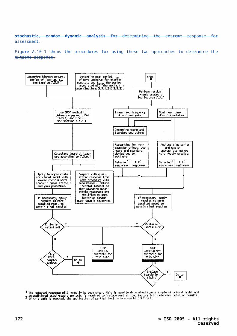
= Fxe for Fy/Fxe 1.911 (A.12.5-6c)
where
Fxe = representative characteristic elastic local buckling strength, in stress units
= 2 Cx E (t / D) (A.12.5-7)
Cx = critical elastic buckling coefficient
The theoretical value of Cx for an ideal tubular is 0.6. However, a reduced value of C x = 0.3 is recommended for use in Equation 12.5-7 to account for the effect of initial geometric imperfections. within tolerance limits given in clause XX. A reduced value of Cx = 0.3 is also implicit in the limits for Fy/Fxe given in Equations 12.5-6.
A.12.5.2.6 Bending
Tubular members subjected to bending forces shall be designed to satisfy the following condition:
M Mb/b (A.12.5-8)
where
M = bending moment due to factored actions
Mb = characteristic bending moment capacity
b = partial resistance factor for bending strength, 1.05.
The representative characteristic bending strength for tubular members should be determined from:
Mb = Mp for (Fy D)/(E t) 0.0517 (A.12.5-9a)
= [1.13 – 2.85 (Fy D)/(E t)] Mp for 0.0517 < (Fy D)/(E t) 0.1034 (A.12.5-9b)
= [0.94 – 0.76 (Fy D)/(E t)] Mp for 0.1034 < (Fy D)/(E t) 120 (Fy / E) (A.12.5-9c)
where
Mp = plastic moment of resistance
= Z Fy
Z = plastic section modulus
= (1/6) [D3 – (D - 2t)3]
My = first yield moment
= S Fy
S = elastic section modulus
= (/64) [D4 – (D-2t)4]/(D/2)
A.12.5.2.7 Beam Shear
Tubular members subjected to beam shear forces shall be designed to satisfy the following condition:
© ISO 2005 – All rights reserved 177

V Fv/v (A.12.5-10)
where
V = beam shear due to factored actions
Fv = representative characteristic shear strength
= A Fy/(23)
A = as defined in 12.5.2.2 << A. ? >>
v = partial resistance factor for beam shear strength, 1.05
A.12.5.2.8 Torsional Shear
Tubular members subjected to torsional shear forces shall be designed to satisfy the following condition:
T Tv/v (A.12.5-11)
where
T = torsional moment due to factored actions
Tv = representative characteristic torsional strength
= 2 Ip Fy/(3 D)
Ip = polar moment of inertia
= ( [D4 – (D - 2t)4]
A.12.5.3 Tubular members subjected to combined forces
A.12.5.3.1 Axial tension and bending
Tubular members subjected to combined axial tension and bending forces shall be designed to satisfy the following condition at all cross sections along their length:
(t Pt / Py) + b (Mby2 + Mbz
2) / Mb] 1.0 (A.12.5-12)
where
Pt, Py, t = as defined in 12.5.2.2 << A. ? >>
Mby, Mbz= bending moments about member y- and z-axes respectively due to factored actions
Mb = as defined in 12.5.2.6 << A. ? >>
b = as defined in 12.5.2.6 << A. ? >>
A.12.5.3.2 Axial compression and bending
Tubular members subjected to combined axial compression and bending forces shall be designed to satisfy the following conditions at all cross sections along their length:
(cPc/Pa) + b/Mb){[ByMby]2 +[BzMbz]2}0.5 1.0 (A.12.5-13)
178 © ISO 2005 – All rights reserved

and
(c Pc/Fyc) + (b /Mb) (Mby2 + Mbz
2)0.5 1.0 (A.12.5-14)
where
Pc, Pa = as defined in 12.5.2.3 << A. ? >>
c = as defined in 12.5.2.3 << A. ? >>
Cmy, Cmz = Moment reduction factors corresponding to the member y and z axes respectively (see 12.5.4) << A. ? >>
My = bending moment about member y-axis due to factored actions
Mz = bending moment about member z-axis due to factored actions
A = as defined in 12.5.2.2 << A. ? >>
Fey, Fez= Euler buckling stresses corresponding to the member y and z axes respectively
Fey = 2 E/(Ky Ly/r)2 (A.12.5-15)
Fez = 2 E/(Kz Lz/r)2 (A.12.5-16)
Ky, Kz = Effective length factors corresponding to the member y and z axes respectively (see 12.5.4) << A. ? >>
Ly, Lz = unbraced length in y or z direction respectively measured between centrelines
r = as defined in 12.5.2.4 << A. ? >>
Mb = as defined in 12.5.2.6 << A. ? >>
b = as defined in 12.5.2.6 << A. ? >>
A.12.6 Strength of Prismatic Members
A.12.6.1 General
The recommendations given in this section apply to rolled and welded prismatic members which may be made up of one or more components such as can be found in a chord section of a jack-up leg. Materials must comply with the general requirements of clause XX and the fabrication must satisfy the tolerance requirements of clause yyy.
Where plating forms one of the components of a cross-section, the yield strength shall be measured both parallel and perpendicular to the direction of rolling and the minimum value adopted. For a rolled section, the yield strength shall be measured in accordance with the relevant standard. The value of yield strength taken from the tensile test shall correspond to the 0.2% offset value and shall not exceed 5/6 th of the ultimate tensile strength. The strain at the ultimate tensile strength should be at least 20 times the strain at the onset of yield.
<<< Maybe insert version of Figure 8.1 here???>>>
<<<8.1.1.1>>>
<<<Maybe insert following as a note??>>>
Code Basis
© ISO 2005 – All rights reserved 179

The main basis for the structural strength check is the AISC 'Load and Resistance Factor Design (LRFD) Specification for Structural Steel Buildings' [14]. The AISC LRFD specification has been interpreted and, in some cases, modified for use in the assessment of mobile jack-up unit structures. Interpretation of the code has been necessary to enable a straight-forward method to be presented for the assessment of beam-columns of non 'I' section. Development of the code has been necessary in two areas as described below:
a) A method has been established for dealing with sections constructed of steels with different material properties.
b) A method has been established for the assessment of beam columns under biaxial bending to overcome a conservatism which has been identified in the standard AISC LRFD equations.
<<<End 8.1.1.1>>>
The resistance factors used in the AISC LRFD specification have been adopted.
In the following sub-sections, x and y are used to define the major and minor axes of a prismatic member.
A.12.6.2 Prismatic members subjected to tension, compression, bending or shear
A.12.6.2.1 General
Non-tubular members subjected independently to axial tension, axial compression, bending or shear should be designed to satisfy the strength and stability requirements specified in 12.6.2.2 to 12.6.2.X.
*****<<Accept Changes and Give All Above To MJRH for Release to WG7 Only>>*****
A.12.6.2.2 Axial Tension
FROM 8.1.4.2
<< ? use P = At * Fymin from 12.3.5.1earlier >>
The nominal tensile strength of a tension component shall be the lower value from the following equations:
a) Pni = FyiAi
b) Pni = FuiAi
where;
Ai = area of component
Fyi = specified minimum yield stress of component (or specified yield strength where no yield point exists)
Fui = specified minimum tensile (ultimate) strength of component
Pni = component nominal axial tensile strength
This assumes that for members in jack-up units the net section is equal to the gross section [Eq's. D1.1 and D1.2].
===============================================================
from 8.1.4.2
180 © ISO 2005 – All rights reserved

A.12.6.2.2.1 Nominal Axial Strength of a Structural Member in tension Pn
For a member comprising more than one component, the nominal tensile strength lies between the maximum individual tensile strength of any one component, and the sum of all the individual tensile strengths.
The total member nominal tensile strength shall be:
Pn = FminAi
with the resistance factor
t = 0.90 [Eq. D1.1]
where Fmin is the smallest value of Fyi or Fui of all the components.
Note: If for any component the nominal strength is significantly different from the nominal strengths of other components, the formulation above may be conservative and alternative rational methods may be applied. An example is given in the Commentary.
<< ? use At from 12.3.5.1earlier >>
A.12.6.2.3 (8.1.4.3 )Nominal Axial Strength of a Structural Member in Compression Pn
So long as local buckling of the components of a member is not the limiting state, the member can be treated for global loads only. Should local buckling dominate, the loads in the components must be considered. Therefore, in determining the nominal axial strength of a member in compression, a local buckling check must first be applied.
Check: Local buckling
The structural components which make up the cross section of a compact or noncompact section must satisfy the following criteria [Table B5.1]:
For a member comprising more than one component, the nominal tensile strength lies between the maximum individual tensile strength of any one component, and the sum of all the individual tensile strengths.
The total member nominal tensile strength shall be:
Pn = FminAi
with the resistance factor
t = 0.90 [Eq. D1.1]
where Fmin is the smallest value of Fyi or Fui of all the components.
Note: If for any component the nominal strength is significantly different from the nominal strengths of other components, the formulation above may be conservative and alternative rational methods may be applied. An example is given in the Commentary.
© ISO 2005 – All rights reserved 181

A.12.6.2.3.1 (8.1.4.3 )Nominal Axial Strength of a Structural Member in Compression Pn
A.12.6.2.3.2 Strength assessment for Compact and Noncompact Sections
The nominal axial strength of a structural member subject to axial compression and within the above stipulated
restrictions regarding cross section shall be determined from the following equations:
<< ? use Ac from 12.3.5.1earlier >>
Pn = A Fcr [Eq. E2.1]
Fcr = (0.658c2) Fyeff For c 1.5 [Eq. E2.2]
Fcr = Fyeff For c > 1.5 [Eq. E2.3]
where;
A = gross area of section (excluding rack teeth of chords)
c = for max. K/r from all directions [Eq. E2.4]
= unbraced length of member:
- face to face for braces
- braced point to braced point for chords
- longer segment length of X-braces (one pair must be in tension, if not braced out of plane)
r = radius of gyration, based on gross area of section.
E = material Young's modulus (200,000 MN/m2 {29,000 ksi}).
Fyeff = effective material yield stress, to be taken as the minimum of (specified) yield stress or 5/6 (ultimate stress) of all components in the member unless rational analysis shows that a higher value may be used.
A.12.6.2.3.3 b) Strength Assessment for Members with Slender Components
The nominal axial strength of a structural member subject to axial compression and outside the restrictions for a) above shall be determined from the following equations.
<< ? use Ay from 12.3.5.x earlier >>
Pn = A Fcr
where;
Fcr = Q(0.658Qc2)Fyeff for c 1.5 [Eq. A-B5-11]
182 © ISO 2005 – All rights reserved

Fcr = Fyeff for c > 1.5 [Eq. A-B5-13]
where c is defined in Section 8.1.4.3 a) and Q is determined from the following:
i) For members comprising entirely of stiffened components [A-B5.3.b and A-B5.3.c]:
Q = Qa
where;
Qa = Ae/A [Eq. A-B5-10]
and
===============================================================
Add SSRC curve ?3? Suggestion is that PAFA and 5-5A may be excessively conservative wrt high strength steel and residual stresses
===============================================================
All assumes low shear (per PAFA). Should include if shear is above 60% of full plastic shear capacity. Incorporated as a simple modifier = 1.0 at < 40% and <1.0 at > 60%
===============================================================
A.12.6.2.4 8.1.4.6 Nominal Bending Strength; Mn (Mnx, Mny)
The calculation of nominal bending strength is based on the plastic properties of the section. The practice allows for hybrid sections built up from components of different yield strengths. Standard techniques shall be applied to obtain a section plastic moment in the absence of axial load, Mp, based on the individual component values which are the lesser values of Fyi and 5/6 Fui (an example is given in the Commentary).
Lateral torsional buckling and local buckling of components must be considered.
If both tensile and compressive yielding occur during the same load cycle, it shall be demonstrated that the structure will shake down without fracture.
a) Compact Sections
The nominal bending strength is given by the plastic bending moment of the whole section
Mn = Mp [Eq-A-F1-1]
where Mp is derived as discussed above.
b) Noncompact Sections
The nominal bending strength is given by an interpolation between the plastic bending moment and the limiting buckling moment:
Mn = Mp - (Mp- Mr) [Eq. A-F1.3]
where;
© ISO 2005 – All rights reserved 183

Mp = Section Plastic Moment.
h = subscript referring to the component which produces the smallest value of Mn.
= b/t or 2R/t as applicable for component h.
p is determined for component h from 8.1.4.6 a).
r is determined for component h from 8.1.4.6 b).
Mr is the limiting buckling moment of the section defined as follows:
For bending of non-tubular sections about the major axis, the lesser of
Mr = Fl S (flange buckling) [Table A-F1.1]
Mr = ReFyfjS (web buckling) [Table A-F1.1]
where;
Fl = the smaller of (Fyfj – Fr) and Fywj
S = minimum section elastic modulus for plane of bending under consideration.
For bending of non-tubular sections about the minor axis;
Mr = FyfjS (flange buckling) [Table A-F1.1]
Fyfj = yield stress of flange component.
Re = hybrid girder reduction factor [A-G2]
= 1.0 if components are of the same material
otherwise:
= [12 + ar (3m – m3)] / (12 + 2 ar) <=1.0
ar = ratio of total web area to area of compression flange.
m = ratio of web component yield stress to flange component yield stress which gives smallest value of Re.
c) Slender Sections
The nominal bending strength of members including components which do not satisfy the above criteria for compact and noncompact sections or for lateral torsional buckling shall be determined in accordance this section.
The nominal bending strength of a member is given by the limiting flexural bending moment:
Mn = S Fcr
where S is the elastic section modulus for the plane of bending under consideration and Fcr is the lowest value from (where appropriate):
i) Doubly symmetric members (lateral torsional buckling)
184 © ISO 2005 – All rights reserved

Fcr = 6.895 [Table A-F1.1(b)]
{Imperial: Fcr = }
where;
Cb = 1.75 + 1.05(M1/M2) + 0.3(M1/M2)2 2.3 where M1 is the smaller and M2 the larger end moment in the unbraced member; M1/M2 is positive when the moments cause reverse curvature. ( 1/MLT in PAFA)
X1 = (/S)
X2 = (4Cw/Iy)(Sx/GJ)2
E = Modulus of elasticity (200,000 MN/m2 {29,000 ksi}).
G = Shear modulus of elasticity (77,200 MN/m2 {11,200 ksi}).
J = Torsion constant for section.
A = Cross-sectional area (excluding rack teeth).
Iy = Second moment of area of section about minor axis.
Sx = Elastic section modulus for major axis bending.
Cw = Warping constant.
= Lb/ry
ry = Radius of gyration about the minor axis
ii) Singly symmetric members (lateral torsional buckling) [Table A-F1.1(c)]
Fcr = {B1 + } Fy
{Imp'l: Fcr = {B1 + } Fy}
where;
B1 = 2.25
B2 = 25
h = web depth.
Ic = second moment of area of compression flange about the section minor axis
Cb = as for doubly symmetric sections.
© ISO 2005 – All rights reserved 185

iii) Doubly and singly symmetric members (flange local buckling)
[Table A-F1.1(g)]
Fcr = 77,220/2 {Imperial: Fcr = 11,200/2}
where;
= bi/ti for flange(s)
A.12.6.2.5
Check: Lateral torsional buckling (Not applicable to tubulars) <<<Paul believes need additional check for non-slender members which can be copy/pasted out of original work>>>
The cross sectional geometry of a member subjected to bending shall be examined for susceptibility to the limit state of lateral torsional bucking. The member cross section must satisfy the following criteria for compact sections for the nominal bending strength to be assessed under Sections 8.1.4.6 a) or 8.1.4.6 b).
Lb/ry 25860 {Imperial: Lb/ry 3750 }
[Table A-F1.1]
where;
Lb = Laterally unbraced length; length between points which are either braced against lateral displacement of the compression flange or braced against twist of the cross section.
ry = Radius of gyration about the minor axis.
A = Cross sectional area.
J = Torsional constant for the section
Sections which do not satisfy this criteria are susceptible to lateral torsional buckling and are treated as having slender compression components as in Section 8.1.4.6 c).
===============================================================
Concern by PAFA that 5-5A does not have suitable lateral torsional buckling checks. Concern that Clause may be misused by people trying to find a fudge system of assessing an odd structure made up of odd sections
===============================================================
A.12.6.2.6
8.1.4 Assessment of Members
8.1.4.1 General interaction equations
Each structural member within the scope of Section 8.1.2 shall satisfy the following conditions:
If Pu/aPn > 0.2
186 © ISO 2005 – All rights reserved

[Eq. H1-1a]
else
[Eq. H1-1b]
where;
Pu = applied axial load
Pn = nominal axial strength determined in accordance with Section 8.1.4.2 (tension) and 8.1.4.3 (compression).
Muex,Muey = effective applied bending moment determined in accordance with Section 8.1.4.4 (tension) and 8.1.4.5 (compression).
<<<May need to add a local strength check here because B has now been allowed to take on a value of <1.0.>>>
===============================================================
from 8.1.4.1
Mnx,Mny = nominal bending strength determined in accordance with Section 8.1.4.6.
a = Resistance factor for axial load = 0.85 for [Eq. E2.1] compression and 0.90 for tension [Eq. D1.1].
b = Resistance factor for bending = 0.9 [Ch. F1.2]
= Exponent for biaxial bending, a constant dependent on the member cross section geometry, determined as follows:
i) For solid or hollow rectangular sections = 5/3
ii) For doubly symmetric open section members, = 1.0
iii) For all other geometries, the value of may be determined by analysis as described in Section 8.1.4.7 but shall not be less than 1.0. In lieu of analysis, a value of equal to 1.0 may be used.
The interaction equations can be used in a reduced form if one or two of the three load ratio terms in the equation are zero.
Note: For purely circular tubular members, = 2.0
Alternatively, the more complex interaction formulations given in Section C8.1.4.7 of the Commentary may be used where applicable.
===============================================================
8.1.4.7 Determination of for non-tubular sections
The general interaction equation requires that applied bending moments are resolved into components in two perpendicular axes (X,Y). For elaborate sections such as chords, these axes may be selected on the basis of section geometry and not on load incidence. Therefore neither of these axes need be coincident with the angle of load. The use of the exponent is necessary to ensure that the effective nominal bending strength of the section is not significantly influenced by this choice of axes.
© ISO 2005 – All rights reserved 187

To determine a suitable value of the following process is applied:
1. For angles q = 0, 30, 45, 60, 90, to the X-axis, obtain the allowable bending strengths Mnq.
2. Assume loads incident at angle q=30, the limiting bending moment in the absence of axial load is Muq
= Mnq. When the section is non-compact Mnq is a function of Mr and a suitable analysis in line with that of Section 8.1.4.6 b), should be applied in determining Mr for non-principal axes.
3. Resolve this limiting moment into limiting components M'uex and M'uey about the X and Y axes:
M'uex = Muq cos q
M'uey = Muq sin q
4. The interaction ratio for the (X,Y) axis pair is required to give the same result as if the X-axis were lined up with the q-axis:
i.e.
Since Mnx and Mny are by definition Mnq for q = 0 and 90 respectively and so are known, the only unknown in the above identity is . This can be determined from the graph in Figure 8.4 or by numerical means if preferred. Figure 8.4 is based on the ratio Muq/Mnq being equal to unity, and will produce conservative results when axial loads are present.
5. Step 4 yields a value of suitable for loads from 30 to the X-axis. Steps 2 to 4 are repeated for q = 45 and 60 to obtain a range of values of .
6. The value of for use in subsequent assessment shall be the least of the above determined values, but not less than 1.0.
This method includes some approximation. Since bending will not be along or perpendicular to a plane of symmetry, deflection will not necessarily be at the same angle as the applied moment. This effect is second order.
Note: An alternative, more detailed approach, involving modified interaction equations is
presented below for a number of typical chord configurations.
===============================================================
C8.1.4.7 Determination of
Determination of the correct value of is carried out by calculation of the nominal strength of the member about axes other than the x- and y-axes. This can be done in the normal manner based on the effective plastic section modulus with reductions for local buckling if applicable. Although a beam will not necessarily bend in the same plane as the applied moment when the bending plane is at an angle to the orthogonal axes, it is not expected that the capacity will be greatly affected.
Once the nominal bending strength has been calculated for a few angles between the x- and y-axes, the value for can be calculated using the graphical procedure given in the practice, or by an iterative procedure. A successful iterative procedure was found to be by the use of the coupled equations, setting a = M'uex/Mnx and b = M'uey/Mny:
i+1 =
with the accelerating step:
i+2 = 0.5(i+1 + i)
188 © ISO 2005 – All rights reserved

and the initial value = 1.5.
The three angles which were chosen, 30, 45 and 60 give a good spread over the 90 range. It is not the intention to fit a curve through all the values from the three angles but merely find the lowest value to . This may still make the equation conservative although considerably less so than for = 1.0.
Plastic Interaction Curve Approach
Alternatively, interaction equations and curves for generic families of chords are presented in Figures C8.1.8 - C8.1.11. The offset distance between the elastic centroid (used in the structural analysis) and the 'center of squash', together with other geometric data for the members of each family of chord is presented in Tables C8.1.1 to C8.1.4.
===============================================================
8.1.4.8 Plastic Interaction Curve Approach
Alternatively, interaction equations and curves for generic families of chords are presented in Figures C8.1.8 - C8.1.11 in the Commentary. These are taken from Dyer [19] and based on the interaction approach proposed by e.g. Duan & Chen [20]. It should be noted that the curves and equations are based on axial load applied at the 'center of squash' which is defined as the location at which the axial load produces no moment on the yielded section. For chords without two axes of symmetry (triangular and tubular with offset rack) this is offset from the elastic centroid when the section is comprised of materials of differing yield strengths. Before a section is checked it is necessary to correct as appropriate moments by the axial load times the offset distance between the elastic centroid (used in the structural analysis) and the 'center of squash'. This offset, together with other geometric data for the members of each family of chord is presented in Tables C8.1.1 to C8.1.4 in the Commentary. The effective applied moment may then be calculated from:
Muex = Bx(Mux + Pu.ey)
Muey = By(Muy + Pu.ex)
The interaction equations are based on ultimate capacity. It is therefore necessary to introduce the required resistance factors. This is achieved by defining:
Py = F1.a.Pn
Mpx = F2.b.Mnx
Mpy = F2.b.Mny
where; F1 = 1.0, unless alternative values are justified by analysis.
F2 = 1.0, unless alternative values are justified by analysis.
The ratio of Pu/Py, Muex/Mpx and Muey/Mpy shall be determined for the condition under consideration. The user should then enter the plastic interaction curves with the Muex/Mpx and Muey/Mpy ratios. The allowable value for Pu/Py may then be determined. A measure of the interaction ratio can then be obtained as the ratio between the actual and allowable values of Pu/Py.
The user should note that the equations for sections with only one axis of symmetry depend on the sign of the moment about the Y-Y axis (given in the Figures). The sign convention should be observed with care.
The equations are based on lower bound data from each family of chord shape and will therefore tend to be conservative. More accurate results will be obtained from the individual consideration of the chord in question.
[NOTE: At present Figures C8.1.8 - C8.1.11 in the Commentary cover only fully plastic section strength considerations, and their use for a beam-column member is based on the assumption that the member being evaluated is sufficiently short/compact that elasto-plastic stability (buckling at large strains) is not a consideration.
© ISO 2005 – All rights reserved 189

Violating this assumption may lead to errors on the unsafe side. Updated information covering elasto-plastic stability may be generated in the future, and should preferentially be used for member evaluations.]
===============================================================
190 © ISO 2005 – All rights reserved

A.13 Acceptance checks
A.13.1 Scope
A.13.2 General formulation
A.13.3 Issues to be assessed
A.13.4 Structural strength checks
A.13.5 Hull elevation
A.13.6 Leg length reserve
A.13.7 Overturning stability
A.13.8 Foundation Integrity
A.13.9 Displacement Check
A.13.10 Temperature
© ISO 2005 – All rights reserved 191

Annex B(informative)
Summary of Load and Resistance Factors
Symbol Description Factor Ref. Clause
f,GAction factor to be applied to the Permanent Action G
1.00 8.7.1
f,Q Action factor to be applied to the Variable Action U 1.00 8.7.1
f,E
Action factor to be applied to the Extreme Environmental Action Ee (used with 50 year independent extreme values)
1.15 8.7.1
f,E
Action factor to be applied to the Extreme Environmental Action Ee (used with 100 year joint probability values)
1.25 8.7.1
f,DAction factor on the Dynamic Action De in combination with f,E
1.00 8.7.1
??? Inertial action induced by the ALE ground motions 0.9 A.10.7
R,NtResistance Factor for prismaticnon-tubular axial tensile loads 1.11 A.12.6
R,NcResistance Factor for prismatic non-tubular axial compressive loads 1.18 A.12.6
R,NbResistance Factor for prismatic non-tubular bending loads 1.11 A.12.6
R,Tt Resistance Factor for tubular axial tensile loads 1.11 A.12.5
R,TcResistance Factor for tubular axial compressive loads 1.18 A.12.5
R,Tb Resistance Factor for tubular bending loads 1.11 A.12.5
R,HResistance Factor for vertical holding system between hull and leg 1.11 13.5
NOTE Values given in this table are for information purposes only. Reference should always be made to the specific clause to ensure that the most up to date values are used.
192 © ISO 2005 – All rights reserved

Annex C(informative)
Response Analysis - Additional Information and Alternative Approaches
© ISO 2005 – All rights reserved 193

Wave reinforcement and cancellation effects << Needs some text and link to Normative or Informative A >>
Figure C.C1 — Periods for wave force cancellation and reinforcement as a function of leg spacing
194 © ISO 2005 – All rights reserved

C.10.4.1.1 - Idealized Single Degree of Freedom System for Natural PeriodsIf such a capability (a finite element structural model containing the mass and stiffness properties of the jack-up) is not available, due to the fact that the mass of the hull dominates the mass distribution, the global dynamic behavior of the jack-up may in some cases be determined from an idealized single degree-of-freedom system and thus the fundamental mode period may be estimated from the system described by:
an equivalent mass representing the mass of the jack-up and its distribution as referred to in Section 7.3.2; (A.10.4.1.2) the equivalent mass is equal to the mass of the hull plus a contribution from the mass of the legs, including added mass, and is located at the center of gravity of the hull.
an equivalent spring representing the combined effect of the overall (global) structural stiffness including stiffness contributions from bending, shear deformation and axial straining of the legs, the leg to hull connections, the hull and the spudcan-foundation interface (if applicable).
The period is determined from the following equation applied to one leg:
Tn = 2
where;
Tn = highest (or first mode) natural period.
Me = effective mass associated with one leg.
= + Mla +
Mhull = full mass of hull including maximum variable load.
N = number of legs.
Mla = mass of leg above lower guide (in the absence of a clamping mechanism) or above the center of the clamping mechanism.
Mlb = mass of leg below the point described for M la, including added mass for the submerged part of the leg ignoring spudcan. The added mass may be determined as A e(CMe - 1) per unit length of one leg (for definitions of Ae and CMe see Section 4.6.6); = mass density of water.
Ke = effective stiffness associated with one leg (for derivation, refer to Commentary).
= *
When the soil rotational stiffness Krs at the spudcan-foundation interface is zero this may be re-written:
© ISO 2005 – All rights reserved 195

Ke = *
Krs = rotational spring stiffness at spudcan-foundation interface.
Krh = rotational stiffness representing leg to hull connection stiffness (see below).
Fr = factor to account for hull bending stiffness.
=
IH = representative second moment of area of the hull girder joining two legs about a horizontal axis normal to the line of environmental action.
E = Young's modulus for steel.
A = axial area of one leg (equals sum of effective chord areas, including a contribution from rack teeth - see Note to Section 5.6.4).
As = effective shear area of one leg (see Figure 5.1).
I = second moment of area of the leg (see Figure 5.1), including a contribution from rack teeth (see Note to Section 5.6.4).
Y = distance between center of one leg and line joining centers of the other two legs (3 leg unit).
= distance between windward and leeward leg rows for direction under consideration (4 leg unit)
Fg = geometric factor.
= 1.125 (3 leg unit), 1.0 (4 leg unit)
Fv = factor to account for vertical soil stiffness, Kvs, and vertical leg-hull connection stiffness, Kvh
(see below).
=
Fh = factor to account for horizontal soil stiffness, Khs, and horizontal leg-hull connection stiffness, Khh (see below).
=
L = length of leg from the seabed reaction point (see Section 5.2.1) to the point separating M1a and M1b (see above).
196 © ISO 2005 – All rights reserved

P = the mean force due to vertical fixed and variable loads acting on one leg.
=
g = acceleration due to gravity.
PE = Euler buckling load of one leg.
= 2EI
= the minimum positive non-zero value of L satisfying:
tan(L) =
Thus:
when Krs = 0 and Krh = , L = /2 and hence:
PE =
when Krs = and Krh = , L = and hence
PE =
The hull to leg connection springs, Krh, Kvh and Khh represent the interaction of the leg with the guides and supporting system and account for local member flexibility and frame action. They should be computed with respect to the point separating M1a and M1b, as described above. The following approximations may be applied:
Khh =
Kvh = effective stiffness due to the series combination of all vertical pinion or fixation system stiffnesses, allowing for combined action with shock-pads, where fitted.
Unit with fixation system:
Krh = combined rotational stiffness of fixation systems on one leg.
= Fnh2kf
where;
Fn = 0.5, three chord leg; = 1.0, four chord leg
h = distance between chord centers.
kf = combined vertical stiffness of all fixation system components on one chord.
Unit without fixation system:
© ISO 2005 – All rights reserved 197

Krh = rotational stiffness allowing for pinion stiffness, leg shear deformation and guide flexibility.
= Fnh2kj +
where;
h = distance between chord centers (opposed pinion chords) or pinion pitch points (single rack chords).
kj = combined vertical stiffness of all jacking system components on one chord.
d = distance between upper and lower guides.
ku = total lateral stiffness of upper guides with respect to lower guides.
As = effective shear area of leg.
The above equations for estimating the fundamental natural period are approximate and ignore the following effects:
more realistic representation of possible fixity at the spudcan-foundation interface in the form of (coupled) horizontal, vertical and rotational spring stiffnesses.
three dimensional influences of the system as compared with the two-dimensional single leg model.
Xxxxxxx
C.1.1.1.1.1 The classical SDOF analogy
This representation assumes that the jack-up on its foundation may be modeled as an equivalent mass-spring-damper mechanism. The (highest) natural period of the vibrational modes may be determined as described in Section A.10.4.1. The torsional mode and corresponding three-dimensional effects cannot be included in this representation.
The single degree-of-freedom (SDOF) method is fundamentally empirical because (1) the wave-current loading does not occur at the mass center and (2) the loading is non-periodic (random) and non-linear. It should also be noted that all global and detailed response parameters are not equally amplified. The method described below will generally lead to a reasonable approximation of the jack-up's real behavior and has been calibrated against more rigorous methods. The following cautions are noted when using the SDOF method:
1) If the ratio of the jack-up natural period to the wave excitation period, , is less than 0.5 and the current is 'relatively small' the SDOF method should give reasonably accurate results when compared to a more rigorous analysis.
2) If is greater than 0.5, the relative position of the jack-up natural period within the base shear transfer function should be checked. If the natural period falls near a wave force peak, then the SDOF method may be unconservative because it ignores forcing at other than the full wave excitation period. Note that the calculation of natural periods should include a range of periods to account for a reasonable estimate of foundation fixity (see Section 7.3.5.2).
3) The SDOF method may be unconservative for cases with relatively high currents. If the results of the assessment are close to the acceptance criteria further detailed analysis is recommended.
198 © ISO 2005 – All rights reserved

The ratio of (the amplitudes of the) dynamic to the quasi-static response as a function of frequency () or period (T) of steady state, periodic and sinusoidal excitation is calculated as the classical dynamic amplification factor (DAF):
DAF =
where;
=
=
= Damping ratio or fraction of critical damping
= (% Critical Damping)/100, 0.07.
T = 0.9Tp.
Tp = most probable peak wave period.
Tn = the jack-up natural period as derived in 7.3.5.
The damping parameter in this model represents the total of all damping contributions (structural, hydrodynamic and soil damping). For the evaluation of extreme response using the SDOF method a value not exceeding 0.07 is recommended.
The calculated DAF from the SDOF method is used to estimate an inertial loadset which represents the contribution of dynamics over and above the quasi-static response in accordance with Figure 7.1. This inertial loadset should be determined as follows and applied at the hull (center of gravity) in the down-wind direction:
Fin = (DAF - 1) BSAmplitude
where;
Fin = Magnitude of the inertial loadset for use in conjunction with the SDOF method.
BSAmplitude = Amplitude of quasi-static Base Shear over one wave cycle.
= (BS(Q - S)Max - BS(Q - S)Min)/2
BS(Q - S)Max = Maximum quasi-static wave/current Base Shear.
BS(Q - S)Min = Minimum quasi-static wave/current Base Shear.
NOTE The above equation is part of a calibrated procedure and should not be altered. A more general inertial loadset procedure, using the results from random analysis, is described in Section 7.3.6.3. (A.10.5.2.1.2)
Xxxxxxxxxxxxxxxxxxxxx
C.10.5.3.2 Methods for determining the MPME
C7.B.2.1 Use of drag-inertia parameter (or equivalent) determined from mean and standard deviation of a frequency or time-domain analysis
© ISO 2005 – All rights reserved 199

This procedure relies on the identification of the two components of the total dynamic response, i.e. the quasi-static and the 'inertial' parts. The 'inertial' part is the amplification of the quasi-static part due to dynamic effects, and should not be confused with inertial wave loading. The procedure requires the determination of the basic statistical parameters of the mean, , and the standard deviation (excluding the mean), , of the required response variable(s). In general the root-mean-square, RMS, , unless = 0. The notation MPMR is used to refer to the most probable value of the response minus the mean response, R(t) - R, for a given storm duration. When the mean is included the MPM value is referred to as the most probable maximum extreme of R(t) and denoted by MPMER.
The response quantity of interest is indicated by the general notation R; this can be any quantity which is related to the random wave excitation (e.g. base shear BS, overturning moment OTM, etc.) Where necessary to distinguish between different forms of response a second subscript is used as follows: 's' for (quasi-)static, 'i' for inertial and 'd' for total dynamic (quasi-static plus inertial) response.
The procedure for estimating the extreme response is shown on Figure C7.B.4, and requires the means and standard deviations of the (overall) dynamic and quasi-static response, and the standard deviation of the 'inertial' response. These can be determined from time domain simulations (Figure C7.B.2) or frequency domain analyses (Figure C7.B.3). Figures C7.B.5 or C7.B.6 form an input to Figure C7.B.4. These Figures are based on [SIPM EPD/51/52 'Dynamic Analysis and Estimation of Extreme Responses for Jack-Ups', August 1991].
C7.B.2.2 Fit Weibull distribution to results of a number of time-domain; simulations to determine responses at required probability level and; average the results.
This procedure requires a suitable length time domain simulation record for each quantity of interest. The input seastate record should be checked for 'Gaussianity'. Guidance is given in Tables 7.2 and 7.3 of the PRACTICE. The procedure requires the following steps.
Step 1
The signal record is first analyzed to calculate the mean, R, as:
where
R(ti) = time history of signal
ti = time points
n = number of useable time points in simulation
(discounting the run-in)
Step 2
The individual point-in-time maxima are next extracted according to the following criteria:
A maximum occurs at ti if:
R(ti-1) < R(ti) and R(ti+1) R(ti)
Suppose Nmax maxima are found in the extraction.
Step 3
200 © ISO 2005 – All rights reserved

From the Nmax maxima, the mean of the signal, R, is subtracted and the maxima R(max,i) are ranked into 20 blocks having mid-points in ascending order. The blocks all have the same width and the upper bound of block 20 is taken as being 1.01 x the largest value, the lower bound of the first block being zero. A distribution of maxima observations is then found, using for each block the Gumbel plotting position in order to obtain the best possible description of the distribution for large values of R. If each block has n i
maxima, the cumulative probability Fi to be plotted against the mid point for block i is then given by:
where n0 = 0.
Step 4.a
A Weibull distribution is fitted against the cumulative distribution of the maxima as defined under Step 3 (see Steps 4.b to 4.d). The 3-parameter Weibull cumulative distribution function is defined as:
F(R;,,) = 1 - exp.
where;
F(R;,,) = probability of non-exceedance
= scale parameter
= slope parameter
= threshold parameter
and ,,(R-) > 0.0
Step 4.b
Only data points R(max,i), corresponding to a probability of non-exceedance greater than a threshold value of 0.2 are used to fit the Weibull distribution, i.e. only the points:
for i>0.2 x Nmax
Notice that R(max,i) are in ascending order.
Step 4.c
For each of these points, the deviations between the Weibull distribution and the values R (max,i)
(transformed to Weibull scales) are calculated as:
i = ln[-ln{1-F(R(max,i),,,)}] - [ln(r(max,i)-) - ln()]
Step 4.d
The parameters ,, are now estimated by a non-linear least square technique, i.e.
© ISO 2005 – All rights reserved 201

is minimized
The procedure may be based on a Levenberg-Marquardt algorithm, using the parameters of a 2-parameter Weibull distribution (found by the maximum likelihood method) as initial estimates.
Step 5
The MPM value RMPM is found as the value of R for which:
F(R,,,) = 1 -
Step 6
The total extreme MPM value, RMPME is found as:
RMPME = R + RMPM
where R = the mean value of R established in Step 1 RMPM = the MPM value (excluding the mean) established in Step 5.
Step 7
The procedure is repeated for each required response parameter.
The basic assumption of this method is that the 3-hour extreme values follow a Gumbel distribution:
C7.B.2.3 Fit Gumbel distribution to histogram of peak responses from a number of time-domain simulations to determine responses at required probability level.
The basic assumption of this method is that the 3-hour extreme values follow a Gumbel distribution:
F3h(x) = exp
where;
F3h(x) = the probability that the 3-hour maximum will not exceed value x.
= location parameter
= scale parameter
The following steps are followed for each required response parameter:
Step 1
Extract maximum (and minimum) value for each of 10 3-hour response signal records.
Step 2
A Gumbel distribution is fitted through these 10 maxima/minima. This is done using the maximum likelihood method, yielding and .
202 © ISO 2005 – All rights reserved

Step 3
The Most Probable Maximum Extreme is found according to:
MPME = - ln
with;
F3h (MPME) = 0.37
The 0.37 lower quantile is used because the extreme of recurrence of once in 3 hours will have a probability of exceedance of 0.63 (= 1 - 0.37). In this case it can be seen that:
MPME =
Step 4
The procedure of Step 3 is similarly applied for minima.
C7.B.2.4 Apply Winterstein's Hermite polynomial method to the results of time domain simulation(s).
For Gaussian processes, analytical results exist for the determination of the MPM values (e.g. MPM wave height = 1.86 x significant wave height). For general non-inear, non-gaussian, finite band-width processes, approximate methods are required to generate the probability density function of the process. The method proposed by Winterstein [Winterstein S.R., 'Non-Linear Vibration Models for Extremes and Fatigue', Journal of Engineering Mechanics, Vol. 114, No 10, 1988] fits a Hermite polynomial of gaussian processes to transform the non-linear, non-gaussian process into a mathematically tractable probability density function. This has been further refined by Jensen [Jensen, J.J. 'Dynamic Amplification of Offshore Steel Platform Responses due to Non-Gaussian Wave Loads', The Danish Center for Applied Mathematics and Mechanics Report No 425, May 1991, Submitted to Journal of Structural Engineering, ASCE] for processes with large kurtosis.
This procedure requires a suitable length time domain simulation record for each quantity of interest. The input seastate record should be checked for 'Gaussianity'. Guidance is given in Tables 7.1 and 7.2 of the PRACTICE. The calculation procedure to determine the maximum of a time series, R(t), in duration T is as follows:
Step 1
Calculate the following quantities of the time series for the parameter under consideration:
= mean of the process
= standard deviation
3 = skewness
4 = kurtosis
Step 2
Hence construct a standardised response process, z = (R - )/. Using this standardised process, calculate the number of zero-upcrossings, N. In lieu of an actual cycle count from the simulated time series, N = 1000 may be assumed for a 3-hour simulation.
Step 3
Compute the following quantities from the characteristics of the response parameters identified earlier:
h3 =
© ISO 2005 – All rights reserved 203

h4 =
K =
It is necessary to seek a more accurate result by determining the solution of the following equations for C1, C2 and C3:
2 = C12 + 6C1C3 + 2C2
2 + 15C32
33 = C2(6C12 + 8C2
2 + 72C1C3 + 270C32)
44 = 60C24 + 3C1
4 + 10395C34 + 60C1
2C22 + 4500C2
2C32 + 630C1
2C32 + 936C1C2
2C3 + 3780C1C3
3 + 60C13C3
using as initial guesses:
C1 = K(1-3h4)
C2 = Kh3
C3 = Kh4
with , K, h3 and h4 from above. Following the solution for C1, C2 and C3, the values for K, h3 and h4 are computed as follows:
K = (C1 + 3C3)/
h3 = C2/(K)
h4 = C3/(K)
Step 4
The most probable value, U, of the transformed process is computed by the following equation:
U =
Where U is a Gaussian process of zero mean, unit variance.
Step 5
The most probable maximum, transformed back to the standardised variable, z, is then given by:
zMPM = K[U + h3(U2 - 1) + h4(U3 - 3U)]
Step 6
Finally, the most probable maximum extreme in the period T, for the response under consideration, can be computed from the following equation:
RMPME = + zMPM
204 © ISO 2005 – All rights reserved

Specific notes with Figure C7.B.2
General
The procedure for estimating the extreme response due to hydrodynamic loading shown in Figure C7.B.4 requires knowledge of the mean and the standard deviation of the quasi-static and dynamic responses, and the standard deviation of the "inertial" response. A time domain procedure may be used to determine these.Re blocks 4, 5, 6: The mean of the "inertial" response is not used in the procedure. In most cases the mean of the static
response will be (approximately) equal to the mean of the dynamic response. Therefore, the mean of the "inertial" response will be (approximately) zero. This may serve as a check on the simulations performed.
However, under certain conditions the means may truly be different. this can most clearly be seen when relative velocities (i.e. the wave induced water particle velocity minus the structure's velocity) are used to perform the dynamic simulation.
Figure C7.B.2 Time domain procedure for determining mean and standard deviation
© ISO 2005 – All rights reserved 205

Specific notes with Figure C7.B.3
General
The procedure for estimating the extreme response due to hydrodynamic loading shown in Figure C7.B.4 requires knowledge of the mean and the standard deviation of the quasi-static and the dynamic responses, and the standard deviation of the "inertial" response. A frequency domain procedure may be used to determine these. In order to reflect the interactions between the current velocity, the absolute wave induced water particle velocity and the structure's velocity (if a relative velocity formulation is adopted) and to linearize the associated drag loading adequately it is necessary to adopt a statistical or least squares linearization procedure as first formulated by Borgman (see Ref. below). Other forms of linearization in frequency domain analysis cannot handle these interactions.
For the least square linearization procedure, there only is a mean response in case of a non-zero current. The magnitude of the mean depends on the value of the current velocity and on the standard deviation of the wave induced (horizontal) water particle velocity, both taken at the same elevation z, and subsequently integrated over the full water depth. The wave induced water particle velocity may be the absolute or the relative velocity, depending on which of these is more appropriate for the case considered.
The transfer functions HRs() and HRd() between the response and the water surface elevation are similarly dependent on both the wave induced (horizontal) absolute or relative velocities and the current velocities at various elevations.
The means mRs and mRd and the transfer functions HRs() and HRd(), are therefore a function of the sea state and the current sued in the environmental definition.Re block 3: The transfer function representing the difference between the dynamic and the quasi-static response is
only notionally associated with "mass inertial" forces (not to be confused with inertial wave loading). The difference may additionally be due to damping forces and any effect causing (frequency dependent) phase differences between HRd() and HRs(). (e.g. associated with multi degree of freedom system responses).
Re blocks 4, 5, 6: The spectral analyses operate on the transfer functions HRx(), which by definition represent the time varying part of the response minus the mean, i.e. Rx(t)-Rx.
A similar note on the mean values of the various responses as given with Figure C7.B.2 should be made here. The mean value of the "inertial" response cannot be determined in a frequency domain analysis and is not required either. However, the fact remains that in most cases the mean of the static response will be (approximately) equal to the mean of the dynamic response. This should again serve as a useful check o the analyses performed.
From the above general note it can be seen that both means will only be non-zero if there is a current present. When relative velocities are used in the analysis of the dynamic problem the interaction
206 © ISO 2005 – All rights reserved

between the current and the relative velocity may be different for the dynamic and the static case, resulting in realistically different mean values.
Reference: L.E. Borgman: "Ocean wave simulation for engineering design" Civil Engineering in the Oceans, ASCE conference, San Francisco, September 1967
Figure C7.B.3 Frequency domain procedure for determining mean and standard deviation
Figure C7.B.4 Procedure for estimating the extreme response
© ISO 2005 – All rights reserved 207

Specific notes with Figure C7.B.4
Re block 7: The correlation coefficient R is theoretically a value between -1 and +1. For virtually all applications to offshore structures problems it is expected that:
2Rd > 2
Rs + 2Ri so that 0 < R < 1.
For rR = 0, zero correlation, the quasi-static and "inertial" responses do not influence one another and will be well separated in the frequency domain. This is generally only to be expected for relatively low natural periods which fall in the (very) high frequency tail of the wave spectrum and where H Rs() is also very low. Under these circumstances the variance (or mean square) of the full dynamic response is equal to the sum of the variances of the quasi-static response and the "inertial" response:
2Rd = 2
Rs + 2Ri
Geometrically, this means a direct addition of non-overlapping areas of the two parts of the response spectrum.
For rR = 1, full correlation, the quasi-static and "inertial" responses are fully dependent on one another. The two parts of the response spectrum overlap strongly and will not really be distinguishable. This will increasingly be the case for high natural periods, considerably closer to the peak of the wave spectrum and therefore associated with a region of significant wave energy, and where HRs() is also having appreciable values. Under these circumstances the standard deviation (instead of the variance) of the full dynamic response is equal to the sum of the standard deviations of the quasi-static response and the "inertial" response:
Rd = Rs + Ri
Re blocks 8, 12, 16: Several definitions of the dynamic amplification factor DAF are in use. The purest and most meaningful definition is believed to be DAF1, the ratio of the standard deviations of the dynamic and static responses (block 8), i.e. after eliminating the means which are not affected by dynamic magnification. If the static and the dynamic processes are both gaussian, or to an equal degree non-gaussian, then DAF2 = DAF1; however, this will not be the case in general. The ratio DAF3 of the most probably maximum extremes, including the means, is a practical overall measure of the increase in response due to dynamics.
Re block 9: The mpm-factor for an arbitrary non-gaussian response is not known. As an engineering postulate it is assumed that this is equal to the mpm-factor for Morison type wave loading on a cylindrical element of unit length. The factor for a nominal number of 1000 peaks (corresponding approximately with a 3 hr storm duration) then varies between the extremes of 3.7 (for inertial wave loading only and hence a gaussian process) and 8.0 (for drag waver loading only and consequently a strongly non-gaussian process). It can be determined on the basis of a drag-inertia parameter or the kurtosis of the response, as shown in Figure C7.B.5 with its associated notes.
Note that the factor 8.0 is different from the previously used factor of 8.6. This is due to the fact that in this report the most probably maximum is consistently used as a predictor for the maximum of a random process. The previous factor 8.6 referred to the expected maximum instead of the most probably maximum.
Re block 10: The mpm-factor for the "inertial" part of the response is associated with the dynamic behavior and predominantly of a purely narrow banded resonant nature. Experience has shown (and theory supports this) that such lightly damped dynamic processes tend towards gaussianity so that a mpm-factor of 3.7 is a reasonable and confident assumption for engineering purposes.
Re block 11: The relationship between the mpm-values is entirely analogous with the relationship between the standard deviations from which the correlation coefficient is determined. However, while it is theoretically proven equation for the standard deviations, it is an engineering postulate for the mpm-values.
Re blocks 14, 15: It should be recalled that the procedure depicted in Figures C7.B.2 to C7.B.6 is aimed at estimating the extreme short-term response due to hydrodynamic loading only (see General Note 1). Therefore, the
208 © ISO 2005 – All rights reserved

effect of wind should be excluded from the most probably maximum extreme static and dynamic responses in block 14 and 15, respectively. Wind is assumed to produce a static load and a static response, and not to influence the dynamic behavior. To determine the ultimate response the mean response due to wind should be determined separately and added to mpmeRs and mpmeRd.
Notes to Figure C7.B.4
Figure C7.B.5 Procedure for determining the mpm-factor of the static response
Specific notes with Figure C7.B.5
Re blocks 9a and 9b: These standard deviations may be obtained from separate time domain simulations in the same manner as shown in Figure C7.B.2 (blocks 1 and 4) or, alternatively, from separate frequency domain analyses as shown in Figure C7.B.3 (blocks 1 and 4). The mean values are not required and neither is it necessary to subtract dynamic and static response time series or transfer functions, respectively.
Re block 9c: The drag-inertia parameter is defined as the ratio of the magnitude of the drag force to the magnitude of the inertia force due to waves. All relationships given below are valid for the case of zero current, which is used as the basis for the whole procedure in view of the engineering approximations involved. For an element of a circular cylinder of diameter D and unit length, subjected to a periodic wave, the drag-inertia parameter then becomes:
© ISO 2005 – All rights reserved 209

K = ( Cd D v2) / ( Cm D2 a)
= (1)
Where v and a are the velocity and the acceleration normal to the element, respectively. As both v and a depend on the wave parameters (wave height, wave period, waterdepth) and the elevation at which the element is located, it is obvious that K is also a function of depth, waterdepth, wave height and wave period. therefore, the theoretical definition of K is only meaningful for Morison wave loading per unit length of the element.
The definition of K can be generalized to random instead of periodic wave conditions by replacing the deterministic normal velocity v by the standard deviation of the random normal velocity v and replacing the deterministic normal acceleration a by the standard deviation of the random normal acceleration a. Equation (1) then becomes:
K = (2)
Using a statistical or least squares linearization procedure in the frequency domain, as developed by Borgman (see notes with Figure C7.B.3), it can be shown that for the wave force on an element of a single member the standard deviations of the two parts of the wave force are as follows:
R(Cm = 0) = 1/2 Cd D.v2
R(Cd = 0) = Cm.1/4 D2.a
These relationships can be used to determine v2 and a, which can then be substituted into equation 2 to
result in:
K = (3)
With R being the wave force per unit length in a random sea.
Equation (3) may subsequently be generalized to apply to any other local or global response R selected for interest. It will be clear that such a generalization is purely an engineering postulate and not founded on theoretical reasoning. It is an attempt to incorporate the important but unknown non-gaussian effects on the maximum response through the assumed similarity with the wave loading process for which the non-gaussian statistics are known.
Yet another way to determine the drag-inertia parameter K for a generalized response R is by using the kurtosis of R. The kurtosis is defined through the expected values of the second and fourth order moments of the time simulations of R, i.e.:
= E {R4} / [E {R2}]2 (4)
For Morison wave loading per unit length of member the relationship between K and the kurtosis k is (see Ref. 2 below):
= (5a)
or in the inverse form:
Notes to Figure C7.B.5
210 © ISO 2005 – All rights reserved

K = (5b)
While K varies between 0 (inertia loading only) and infinity (drag loading only) ranges from 3 to 35/3. It may now be assumed that the same relationship holds for an arbitrary response variable R. Therefore, if the kurtosis of R is know the corresponding drag-inertia parameter K can be determined. If this is done, separate time domain simulations for the standard deviations in blocks 9a and 9b are not required but the route through block 93 cannot be followed. One enters the diagram in block 9c and must read CRs from Figure C7.B.6 as per block 9d.
Both the kurtosis and the drag-inertia parameter may be subject to appreciable statistical variability and their determination may require time domain simulations of substantial length; see Ref. 2 below.
Re blocks 9d and 9e: Figure C7.B.6 (referred to in block 9d) is equivalent to the figure that was derived by Brouwers and Verbeek and presented in Ref. 1 below as well as in Figure A1 of the SIPM - Practice (EP 89-0550). However, this latter figure presented the ratio of the expected value of the extreme to the standard deviation for a 1000 peaks, rather than the mpm-factor CR which is the ratio of the most probable maximum value of the response to the standard deviation, which is used in this report. Therefore, Figure C7.B.6 has been recalculated in accordance with Ref. 3 and now truly presents the mpm-factor CR. It should be noted that the figure is valid for a narrow band process, the corresponding ratios for a broad band process being somewhat smaller. Therefore, CR is a slightly conservative estimate for the mpm-factor. This is in accordance with the general principles underlying a simplified engineering method and is well within the accuracy of the overall procedure.
An alternative and practical method to estimate K is to apply the engineering assumption for estimating the most probably maximum value of the dynamic response, as used in block 11 of Figure C7.B.4, to separate responses due to hydrodynamic drag loading only and inertia loading only, replacing RS from block 9 and Ri from block 10, respectively. These two hydrodynamic loading components are fully uncorrelated and so are the responses caused by them; hence the correlation coefficient r = 0. Further, the mpm-factor for a totally drag dominated Morison force is 8.0 and for a totally inertia dominated Morison force it is 3.7. With these substitutions the equation in block 11 of Figure C7.B.4 becomes:
mpmR2 = {8.0 R (Cm = 0)}2 + {3.7 R (Cd = 0)}2
For zero correlation the standard deviation of the overall response is obtained from the equation:
R2 = {R (Cm = 0)}2 + {R (Cd = 0)}2
(see note with block 7 of Figure C7.B.4).
These are the equations presented in block 9e. The comments made with regard to conservatism included in the route through block 9d remain equally valid here.
Its determination in block 9c could therefore, strictly speaking be avoided. The input of KRs into block 93 of Figure C7.B.5 is symbolic, representing the implicit use through Rs (Cm = 0) and Rs (Cd = 0), resulting directly from blocks 9a and 9b. In practical applications it is recommended that both routes through block 9d and 93 are followed as a check on the calculations.
Reference 1: J.J.H. Brouwers and P.H.J. Verbeek, "Expected fatigue damage and expected extreme response for Morison-type wave loading", Applied Ocean Research, Vol. 5, No. 3, 1983, pp. 129-133
Reference 2: P.M. Hagemeijer, "Estimation of drag/inertia parameters using time-domain simulations and the prediction of the extreme response", Applied Ocean Research, Vol. 12, No. 3, 1990, pp. 134-140.
Reference 3: J.J.M. Baar, Extreme values of Morison-type processes", Report EP 90-33365, October 1990. To be published shortly in Applied Ocean Research
Notes to Figure C7.B.5 (cont.)
© ISO 2005 – All rights reserved 211

The equation for the curve is Ref. 3, Specific notes with Fig. C7.B.5
Where A, B, C and D are functions of k as follows:
A = 3K2 + 1
B =
C =
D = 1/(8K2)
Figure C7.B.6 Ratio C R of most probable maximum to standard deviation as a function of drag-inertia parameter K for N = 1000 peaks
212 © ISO 2005 – All rights reserved

Figure C7.B.7 Comparison between the normalized spectra S ( ), S ( ) and S PM( )
© ISO 2005 – All rights reserved 213

Annex D(informative)
Foundations - Additional Information and Alternative Approaches
214 © ISO 2005 – All rights reserved
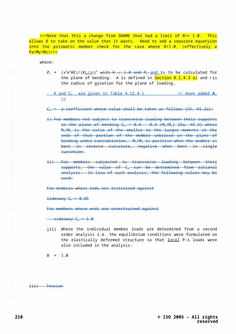
D.9.3.2.3 Penetration in clays << Note to P4 -inserted as Word Tables per ISO re translation, etc. >>
30 degrees cones FV/(Acuo) factors
2R D cuo 2R Roughness
cum R cum cuo 0.0 0.2 0.4 0.6 0.8 1.0
0.0 0.0 1.00 0.00 4.61 5.51 6.38 7.22 8.03 8.78
0.0 0.2 1.00 0.00 4.80 5.70 6.56 7.40 8.20 8.95
0.0 0.5 1.00 0.00 5.05 5.94 6.80 7.63 8.43 9.18
0.0 1.0 1.00 0.00 5.41 6.29 7.14 7.79 8.76 9.50
0.0 2.0 1.00 0.00 5.98 6.85 7.70 8.51 9.29 10.03
0.0 5.0 1.00 0.00 7.12 7.98 8.81 9.61 10.38 11.10
1.0 0.0 1.00 1.00 7.53 9.02 10.46 11.84 13.19 14.46
1.0 0.2 1.10 0.91 7.45 8.89 10.27 11.61 12.90 14.13
1.0 0.5 1.25 0.80 7.38 8.73 10.05 11.32 12.55 13.72
1.0 1.0 1.50 0.67 7.28 8.55 9.78 10.98 12.14 13.24
1.0 2.0 2.00 0.50 7.20 8.38 9.51 10.61 11.68 12.68
1.0 5.0 3.50 0.29 7.34 8.39 9.39 10.37 11.30 12.19
2.0 0.0 1.00 2.00 10.45 12.51 14.51 16.44 18.31 20.10
2.0 0.2 1.20 1.67 9.65 11.53 13.33 15.08 16.79 18.40
2.0 0.5 1.50 1.33 8.89 10.58 12.19 13.76 15.27 16.72
2.0 1.0 2.00 1.00 8.20 9.67 11.09 12.47 13.80 15.08
2.0 2.0 3.00 0.67 7.60 8.87 10.10 11.30 12.45 13.54
2.0 5.0 6.00 0.33 7.37 8.44 9.48 10.18 11.44 12.35
3.0 0.0 1.00 3.00 13.36 15.98 18.56 21.03 23.42 25.71
3.0 0.2 1.30 2.31 11.51 13.76 15.92 18.02 20.05 22.00
3.0 0.5 1.75 1.71 9.98 11.89 13.72 15.49 17.21 18.85
3.0 1.0 2.50 1.20 8.74 10.33 11.87 13.36 14.80 16.18
3.0 2.0 4.00 0.75 7.79 9.11 10.39 11.64 12.83 13.98
3.0 5.0 8.50 0.35 7.40 8.46 9.51 10.52 11.49 12.42
4.0 0.0 1.00 4.00 16.27 19.46 22.57 25.62 28.52 31.32
4.0 0.2 1.40 2.86 13.10 15.68 18.14 20.54 22.86 25.08
4.0 0.5 2.00 2.00 10.83 12.87 14.86 16.79 18.66 20.44
4.0 1.0 3.00 1.33 9.11 10.77 12.38 13.96 15.47 16.91
4.0 2.0 5.00 0.80 7.91 9.26 10.57 11.84 13.06 14.23
4.0 5.0 11.00 0.36 7.40 8.47 9.52 10.54 11.52 12.46
5.0 0.0 1.00 5.00 19.18 22.94 26.61 30.20 33.63 36.92
5.0 0.2 1.50 3.33 14.48 17.33 20.06 22.72 25.29 27.75
5.0 0.5 2.25 2.22 11.46 13.64 15.75 17.80 19.78 21.68
5.0 1.0 3.50 1.43 9.37 11.08 12.77 14.38 15.94 17.43
5.0 2.0 6.00 0.83 7.98 9.35 10.68 11.97 13.21 14.40
5.0 5.0 13.50 0.37 7.40 8.47 9.53 10.56 11.55 12.48
60 degrees cones FV/(Acuo) factors
© ISO 2005 – All rights reserved 215

2R D cuo 2R Roughnesscum R cum cuo 0.0 0.2 0.4 0.6 0.8 1.0
0.0 0.0 1.00 0.00 4.45 4.96 5.45 5.90 6.32 6.69
0.0 0.2 1.00 0.00 4.68 5.19 5.67 6.12 6.53 6.90
0.0 0.5 1.00 0.00 4.98 5.50 5.96 6.40 6.81 7.18
0.0 1.0 1.00 0.00 5.41 5.90 6.37 6.81 7.21 7.57
0.0 2.0 1.00 0.00 6.07 6.55 7.01 7.43 7.84 8.18
0.0 5.0 1.00 0.00 7.33 7.81 8.25 8.66 9.05 9.39
1.0 0.0 1.00 1.00 5.81 6.51 7.15 7.77 8.34 8.87
1.0 0.2 1.10 0.91 5.92 6.59 7.23 7.83 8.38 8.89
1.0 0.5 1.25 0.80 6.04 6.70 7.30 7.88 8.42 8.91
1.0 1.0 1.50 0.67 6.20 6.84 7.41 7.96 8.47 8.94
1.0 2.0 2.00 0.50 6.43 7.05 7.58 8.12 8.59 9.03
1.0 5.0 3.50 0.29 6.97 7.55 8.08 8.54 8.98 9.39
2.0 0.0 1.00 2.00 7.14 8.02 8.84 9.60 10.32 10.99
2.0 0.2 1.20 1.67 6.92 7.73 8.49 9.21 9.88 10.50
2.0 0.5 1.50 1.33 6.74 7.50 8.18 8.84 9.46 10.03
2.0 1.0 2.00 1.00 6.59 7.29 7.91 8.53 9.09 9.61
2.0 2.0 3.00 0.67 6.55 7.20 7.76 8.33 8.83 9.30
2.0 5.0 6.00 0.33 6.99 7.49 8.03 8.50 8.95 9.37
3.0 0.0 1.00 3.00 8.49 9.54 10.50 11.42 12.29 13.10
3.0 0.2 1.30 2.31 7.77 8.70 9.56 10.38 11.14 11.85
3.0 0.5 1.75 1.71 7.24 8.03 8.80 9.53 10.20 10.82
3.0 1.0 2.50 1.20 6.82 7.56 8.21 8.86 9.45 10.00
3.0 2.0 4.00 0.75 6.60 7.27 7.85 8.44 8.94 9.43
3.0 5.0 8.50 0.35 6.99 7.47 8.01 8.49 8.94 9.36
4.0 0.0 1.00 4.00 9.83 11.02 12.16 13.24 14.26 15.18
4.0 0.2 1.40 2.86 8.51 9.52 10.48 11.38 12.22 13.00
4.0 0.5 2.00 2.00 7.61 8.44 9.26 10.04 10.75 11.41
4.0 1.0 3.00 1.33 6.97 7.74 8.41 9.08 9.69 10.26
4.0 2.0 5.00 0.80 6.64 7.31 7.90 8.49 9.01 9.51
4.0 5.0 11.00 0.36 6.86 7.45 8.00 8.48 8.94 9.35
5.0 0.0 1.00 5.00 11.17 12.52 13.83 15.06 16.20 17.26
5.0 0.2 1.50 3.33 9.14 10.23 11.26 12.25 13.15 13.99
5.0 0.5 2.25 2.22 7.90 8.78 9.63 10.43 11.17 11.87
5.0 1.0 3.50 1.43 7.08 7.84 8.55 9.24 9.86 10.45
5.0 2.0 6.00 0.83 6.66 7.32 7.94 8.53 9.06 9.56
5.0 5.0 13.50 0.37 6.85 7.44 7.99 8.47 8.93 9.35
216 © ISO 2005 – All rights reserved

90 degrees cones FV/(Acuo) factors
2R D cuo 2R Roughnesscum R cum cuo 0.0 0.2 0.4 0.6 0.8 1.0
0.0 0.0 1.00 0.00 4.64 5.02 5.36 5.67 5.95 6.17
0.0 0.2 1.00 0.00 4.90 5.28 5.61 5.91 6.18 6.41
0.0 0.5 1.00 0.00 5.22 5.59 5.93 6.23 6.49 6.71
0.0 1.0 1.00 0.00 5.68 6.03 6.36 6.66 6.92 7.14
0.0 2.0 1.00 0.00 6.37 6.71 7.05 7.32 7.58 7.79
0.0 5.0 1.00 0.00 7.65 8.03 8.32 8.60 8.86 9.05
1.0 0.0 1.00 1.00 5.57 6.05 6.47 6.87 7.22 7.53
1.0 0.2 1.10 0.91 5.74 6.21 6.62 7.00 7.36 7.65
1.0 0.5 1.25 0.80 5.94 6.38 6.79 7.16 7.50 7.79
1.0 1.0 1.50 0.67 6.16 6.61 6.99 7.36 7.68 7.97
1.0 2.0 2.00 0.50 6.50 6.93 7.30 7.64 7.95 8.21
1.0 5.0 3.50 0.29 7.25 7.57 7.94 8.25 8.53 8.78
2.0 0.0 1.00 2.00 6.46 7.03 7.54 8.01 8.45 8.82
2.0 0.2 1.20 1.67 6.41 6.94 7.43 7.88 8.28 8.65
2.0 0.5 1.50 1.33 6.41 6.88 7.35 7.76 8.14 8.46
2.0 1.0 2.00 1.00 6.40 6.88 7.29 7.69 8.03 8.35
2.0 2.0 3.00 0.67 6.54 6.99 7.37 7.73 8.06 8.33
2.0 5.0 6.00 0.33 7.16 7.49 7.86 8.18 8.47 8.72
3.0 0.0 1.00 3.00 7.36 8.00 8.59 9.14 9.65 10.08
3.0 0.2 1.30 2.31 6.99 7.57 8.10 8.60 9.05 9.45
3.0 0.5 1.75 1.71 6.70 7.24 7.73 8.17 8.59 8.94
3.0 1.0 2.50 1.20 6.54 7.04 7.47 7.88 8.24 8.57
3.0 2.0 4.00 0.75 6.56 7.02 7.41 7.78 8.11 8.39
3.0 5.0 8.50 0.35 7.12 7.46 7.83 8.15 8.44 8.46
4.0 0.0 1.00 4.00 8.22 8.96 9.64 10.25 10.82 11.33
4.0 0.2 1.40 2.86 7.49 8.11 8.68 9.22 9.70 10.14
4.0 0.5 2.00 2.00 6.94 7.50 8.01 8.48 8.92 9.29
4.0 1.0 3.00 1.33 6.63 7.15 7.58 8.01 8.38 8.72
4.0 2.0 5.00 0.80 6.57 7.03 7.43 7.80 8.14 8.42
4.0 5.0 11.00 0.36 7.05 7.44 7.81 8.13 8.42 8.67
5.0 0.0 1.00 5.00 9.11 9.93 10.66 11.35 12.00 12.56
5.0 0.2 1.50 3.33 7.87 8.55 9.17 9.74 10.26 10.75
5.0 0.5 2.25 2.22 7.12 7.71 8.24 8.72 9.17 9.57
5.0 1.0 3.50 1.43 6.70 7.22 7.67 8.09 8.47 8.82
5.0 2.0 6.00 0.83 6.57 7.04 7.44 7.82 8.16 8.44
5.0 5.0 13.50 0.37 7.03 7.42 7.80 8.12 8.41 8.66
© ISO 2005 – All rights reserved 217
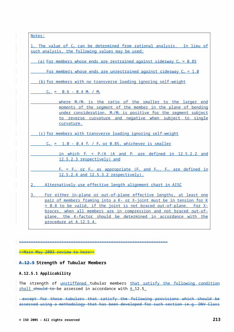
120 degrees cones FV/(Acuo) factors
2R D cuo 2R Roughnesscum R cum cuo 0.0 0.2 0.4 0.6 0.8 1.0
0.0 0.0 1.00 0.00 4.96 5.25 5.51 5.73 5.92 6.05
0.0 0.2 1.00 0.00 5.23 5.52 5.77 5.99 6.17 6.30
0.0 0.5 1.00 0.00 5.57 5.85 6.10 6.31 6.49 6.62
0.0 1.0 1.00 0.00 6.04 6.31 6.55 6.76 6.93 7.05
0.0 2.0 1.00 0.00 6.74 7.01 7.24 7.44 7.61 7.72
0.0 5.0 1.00 0.00 8.07 8.32 8.55 8.75 8.90 8.99
1.0 0.0 1.00 1.00 5.69 6.04 6.36 6.65 6.89 7.09
1.0 0.2 1.10 0.91 5.89 6.24 6.55 6.82 7.07 7.26
1.0 0.5 1.25 0.80 6.12 6.45 6.76 7.02 7.26 7.45
1.0 1.0 1.50 0.67 6.39 6.72 7.01 7.27 7.48 7.66
1.0 2.0 2.00 0.50 6.80 7.10 7.37 7.61 7.82 7.97
1.0 5.0 3.50 0.29 7.52 7.82 8.08 8.29 8.49 8.61
2.0 0.0 1.00 2.00 6.38 6.79 7.16 7.50 7.80 8.04
2.0 0.2 1.20 1.67 6.41 6.80 7.16 7.47 7.75 7.97
2.0 0.5 1.50 1.33 6.46 6.83 7.17 7.46 7.72 7.94
2.0 1.0 2.00 1.00 6.56 6.91 7.22 7.49 7.74 7.92
2.0 2.0 3.00 0.67 6.80 7.12 7.40 7.65 7.87 8.03
2.0 5.0 6.00 0.33 7.43 7.72 7.99 8.21 8.41 8.53
3.0 0.0 1.00 3.00 7.04 7.51 7.93 8.31 8.66 8.93
3.0 0.2 1.30 2.31 6.84 7.27 7.65 8.00 8.31 8.57
3.0 0.5 1.75 1.71 6.71 7.09 7.45 7.76 8.05 8.27
3.0 1.0 2.50 1.20 6.66 7.02 7.34 7.63 7.88 8.08
3.0 2.0 4.00 0.75 6.81 7.11 7.41 7.67 7.89 8.06
3.0 5.0 8.50 0.35 7.38 7.68 7.95 8.17 8.38 8.51
4.0 0.0 1.00 4.00 7.70 8.22 8.69 9.11 9.49 9.81
4.0 0.2 1.40 2.86 7.20 7.66 8.07 8.44 8.77 9.03
4.0 0.5 2.00 2.00 6.88 7.28 7.65 7.98 8.27 8.53
4.0 1.0 3.00 1.33 6.72 7.08 7.42 7.71 7.97 8.18
4.0 2.0 5.00 0.80 6.80 7.12 7.41 7.68 7.90 8.08
4.0 5.0 11.00 0.36 7.39 7.66 7.93 8.15 8.36 8.49
5.0 0.0 1.00 5.00 8.35 8.91 9.43 9.89 10.31 10.67
5.0 0.2 1.50 3.33 7.52 7.99 8.43 8.82 9.18 9.95
5.0 0.5 2.25 2.22 7.01 7.43 7.81 8.15 8.45 8.72
5.0 1.0 3.50 1.43 6.77 7.13 7.47 7.77 8.03 8.25
5.0 2.0 6.00 0.83 6.80 7.12 7.42 7.69 7.91 8.09
5.0 5.0 13.50 0.37 7.34 7.64 7.91 8.14 8.34 8.48
218 © ISO 2005 – All rights reserved

150 degrees cones FV/(Acuo) factors
2R D cuo 2R Roughnesscum R cum cuo 0.0 0.2 0.4 0.6 0.8 1.0
0.0 0.0 1.00 0.00 5.32 5.55 5.74 5.89 6.01 6.05
0.0 0.2 1.00 0.00 5.60 5.82 6.00 6.16 6.26 6.30
0.0 0.5 1.00 0.00 5.94 6.16 6.34 6.49 6.59 6.61
0.0 1.0 1.00 0.00 6.41 6.62 6.80 6.94 7.03 7.05
0.0 2.0 1.00 0.00 7.13 7.32 7.49 7.62 7.71 7.72
0.0 5.0 1.00 0.00 8.46 8.65 8.81 8.93 8.99 8.99
1.0 0.0 1.00 1.00 5.94 6.22 6.46 6.67 6.84 6.97
1.0 0.2 1.10 0.91 6.16 6.43 6.67 6.87 7.04 7.15
1.0 0.5 1.25 0.80 6.41 6.67 6.90 7.09 7.25 7.36
1.0 1.0 1.50 0.67 6.71 6.96 7.18 7.36 7.51 7.60
1.0 2.0 2.00 0.50 7.13 7.36 7.57 7.73 7.86 7.95
1.0 5.0 3.50 0.29 7.91 8.12 8.31 8.44 8.56 8.61
2.0 0.0 1.00 2.00 6.50 6.82 7.11 7.35 7.57 7.73
2.0 0.2 1.20 1.67 6.59 6.90 7.16 7.40 7.59 7.74
2.0 0.5 1.50 1.33 6.69 6.98 7.23 7.45 7.63 7.76
2.0 1.0 2.00 1.00 6.84 7.10 7.34 7.54 7.70 7.82
2.0 2.0 3.00 0.67 7.11 7.35 7.57 7.74 7.89 7.99
2.0 5.0 6.00 0.33 7.81 8.01 8.21 8.35 8.47 8.53
3.0 0.0 1.00 3.00 7.03 7.40 7.72 7.98 8.24 8.43
3.0 0.2 1.30 2.31 6.94 7.27 7.56 7.81 8.03 8.21
3.0 0.5 1.75 1.71 6.88 7.18 7.45 7.68 7.88 8.03
3.0 1.0 2.50 1.20 6.91 7.18 7.43 7.63 7.81 7.94
3.0 2.0 4.00 0.75 7.10 7.35 7.57 7.75 7.90 8.00
3.0 5.0 8.50 0.35 7.76 7.97 8.16 8.31 8.43 8.49
4.0 0.0 1.00 4.00 7.55 7.94 8.30 8.58 8.88 9.10
4.0 0.2 1.40 2.86 7.23 7.58 7.89 8.16 8.40 8.59
4.0 0.5 2.00 2.00 7.02 7.34 7.62 7.86 8.07 8.23
4.0 1.0 3.00 1.33 6.95 7.23 7.49 7.70 7.88 8.01
4.0 2.0 5.00 0.80 7.09 7.34 7.56 7.75 7.90 8.00
4.0 5.0 11.00 0.36 7.72 7.94 8.13 8.29 8.41 8.47
5.0 0.0 1.00 5.00 8.05 8.48 8.86 9.19 9.48 9.74
5.0 0.2 1.50 3.33 7.46 7.83 8.16 8.44 8.69 8.90
5.0 0.5 2.25 2.22 7.13 7.45 7.74 7.99 8.20 8.37
5.0 1.0 3.50 1.43 6.99 7.27 7.53 7.74 7.93 8.07
5.0 2.0 6.00 0.83 7.09 7.34 7.56 7.75 7.91 8.01
5.0 5.0 13.50 0.37 7.70 7.93 8.12 8.27 8.40 8.46
© ISO 2005 – All rights reserved 219

180 degrees cones FV(Acuo) factors
2R D cuo 2R Roughnesscum R cum cuo 0.0 0.2 0.4 0.6 0.8 1.0
0.0 0.0 1.00 0.00 5.69 5.86 5.97 6.03 6.05 6.05
0.0 0.2 1.00 0.00 5.97 6.13 6.24 6.29 6.30 6.30
0.0 0.5 1.00 0.00 6.31 6.47 6.57 6.61 6.61 6.61
0.0 1.0 1.00 0.00 6.79 6.93 7.02 7.05 7.05 7.05
0.0 2.0 1.00 0.00 7.49 7.63 7.70 7.71 7.71 7.71
0.0 5.0 1.00 0.00 8.82 8.94 8.99 8.99 8.99 8.99
1.0 0.0 1.00 1.00 6.25 6.47 6.65 6.79 6.90 6.95
1.0 0.2 1.10 0.91 6.48 6.69 6.87 7.00 7.10 7.14
1.0 0.5 1.25 0.80 6.74 6.94 7.11 7.23 7.32 7.35
1.0 1.0 1.50 0.67 7.05 7.24 7.39 7.51 7.58 7.60
1.0 2.0 2.00 0.50 7.47 7.64 7.79 7.88 7.93 7.94
1.0 5.0 3.50 0.29 8.26 8.32 8.52 8.60 8.61 8.61
2.0 0.0 1.00 2.00 6.73 6.98 7.20 7.39 7.53 7.63
2.0 0.2 1.20 1.67 6.85 7.08 7.30 7.46 7.59 7.68
2.0 0.5 1.50 1.33 6.98 7.20 7.39 7.55 7.66 7.72
2.0 1.0 2.00 1.00 7.15 7.36 7.53 7.67 7.76 7.80
2.0 2.0 3.00 0.67 7.45 7.63 7.78 7.90 7.96 7.98
2.0 5.0 6.00 0.33 8.16 8.27 8.43 8.50 8.53 8.53
3.0 0.0 1.00 3.00 7.16 7.45 7.69 7.91 8.08 8.21
3.0 0.2 1.30 2.31 7.13 7.40 7.62 7.81 7.96 8.07
3.0 0.5 1.75 1.71 7.15 7.37 7.58 7.75 7.88 7.96
3.0 1.0 2.50 1.20 7.21 7.42 7.61 7.75 7.86 7.91
3.0 2.0 4.00 0.75 7.43 7.62 7.78 7.90 7.97 7.99
3.0 5.0 8.50 0.35 8.13 8.23 8.38 8.46 8.49 8.49
4.0 0.0 1.00 4.00 7.56 7.87 8.15 8.38 8.58 8.73
4.0 0.2 1.40 2.86 7.38 7.64 7.89 8.09 8.26 8.39
4.0 0.5 2.00 2.00 7.26 7.50 7.71 7.89 8.03 8.13
4.0 1.0 3.00 1.33 7.25 7.46 7.65 7.80 7.92 7.98
4.0 2.0 5.00 0.80 7.44 7.61 7.77 7.89 7.97 8.00
4.0 5.0 11.00 0.36 8.09 8.19 8.36 8.44 8.47 8.47
5.0 0.0 1.00 5.00 7.94 8.27 8.57 8.83 9.05 9.23
5.0 0.2 1.50 3.33 7.56 7.85 8.10 8.32 8.50 8.64
5.0 0.5 2.25 2.22 7.34 7.59 7.81 8.00 8.15 8.25
5.0 1.0 3.50 1.43 7.27 7.49 7.68 7.84 7.96 8.02
5.0 2.0 6.00 0.83 7.43 7.60 7.77 7.89 7.97 8.00
5.0 5.0 13.50 0.37 8.07 8.18 8.35 8.43 8.46 8.46
220 © ISO 2005 – All rights reserved

D.9.3.2.4 Penetration in silica sands
Commentary: (MC to move this to Annex D with some additional write-up on conical angle)
Values of :
Various bearing capacity and shape factors are given in the literature for the analysis of bearing capacity in silica sands. Traditionally, the value of the dimensionless bearing capacity has been calculated for strip footings, and applied to circular foundations by using an empirical shape factor. However, more recently values for the axisymmetric case have been directly determined. Recent tabulated lower bound solutions have been provided by Cassidy and Houlsby (2002) for circular conical foundations of radius, R, cone angles between 30 and 180 (flat plate), a range of roughness from smooth to fully rough and angles of friction () between 5 and 50. Other values for rough circular footings have been provided by Martin (2004) and are discussed in the context of the load carrying capacity of foundation by Randolph et al. (2004). For the rough circular plate the suggested values of Martin (2004) are given in Table C9.3-1.
Table D.9.3-1 Bearing capacity factors for circular rough plate (Martin, 2004)
Friction angle
: degrees
Bearing factor, Nγ
Bearing factor,
Nq
5 0.081 1.71
10 0.32 2.96
15 0.93 5.25
20 2.42 9.61
25 6.07 18.4
30 15.5 37.2
35 41.9 80.8
40 124 193
45 418 521
The factors of Cassidy and Houlsby (2002) have been derived for the problem defined in Figure D9.4.1 (friction angle, ; radius, R; cone apex angle, β; roughness factor α, such that the interface friction angle δ is given by tanδ = αtan). The dimensionless bearing capacity values of Cassidy and Houlsby are detailed in Tables D9.3.2 to D9.3.7.
Figure D.9.3-1 – Definition of parameters for Tables D.9.3.2 to D.9.3.7
© ISO 2005 – All rights reserved 221
footing roughness
FV
homogeneous soil
R

needs to be addressed due to overlapped uses.Table D.9.3-2 – Bearing capacity factors (N) for a conical apex angle of 30°
= 30°
(°) = 1 = 0.8 = 0.6 = 0.4 = 0.2 = 0
5 2.626 2.483 2.333 2.183 2.028 1.870
10 5.290 4.821 4.324 3.823 3.318 2.825
15 10.49 9.307 7.987 6.712 5.482 4.294
20 20.86 18.08 15.10 12.09 9.232 6.619
25 42.39 36.07 29.08 22.18 15.70 10.15
30 89.80 75.22 58.92 42.45 29.05 16.26
35 203.4 166.2 132.8 84.73 53.14 25.82
40 504.1 410.7 295.4 183.7 101.3 45.24
45 1420.3 1149.1 787.5 417.3 211.7 74.34
50 6504.3 3871.1 2567.7 1388.2 562.1 145.0
Table D.9.3-2 – Bearing capacity factors (N) for a conical apex angle of 60°
= 60°
(°) = 1 = 0.8 = 0.6 = 0.4 = 0.2 = 0
5 1.073 1.036 0.995 0.953 0.909 0.863
10 1.999 1.872 1.735 1.591 1.446 1.299
15 3.775 3.445 3.080 2.708 2.340 1.979
20 7.333 6.546 5.639 4.752 3.896 3.075
25 14.69 12.99 10.94 8.660 6.639 4.820
30 31.99 27.45 22.50 16.70 11.86 7.950
35 79.26 62.95 48.81 34.83 22.57 13.36
40 209.2 163.2 122.3 80.13 47.27 23.75
45 646.3 495.8 382.4 214.1 108.0 46.05
50 2650.0 1913.2 1414.7 698.1 295.3 108.8
Table D.9.3-4 – Bearing capacity factors (N) for a conical apex angle of 90°
= 90°
(°) = 1 = 0.8 = 0.6 = 0.4 = 0.2 = 0
5 0.625 0.605 0.586 0.565 0.544 0.521
10 1.175 1.113 1.044 0.972 0.896 0.818
15 2.269 2.100 1.909 1.709 1.540 1.313
20 4.540 4.114 3.625 3.114 2.600 2.115
25 9.581 8.502 7.257 5.936 4.663 3.509
30 21.12 18.87 15.58 12.09 8.911 6.219
35 51.76 47.42 37.01 26.95 18.26 11.26
40 142.8 132.6 99.18 67.48 40.80 22.13
45 458.7 419.5 312.6 199.6 107.1 51.30
50 1923.3 1850.4 1384.0 751.8 340.1 115.2
222 © ISO 2005 – All rights reserved

Table D.9.3-5 – Bearing capacity factors (N) for a conical apex angle of 120°
= 120°
(°) = 1 = 0.8 = 0.6 = 0.4 = 0.2 = 0
5 0.386 0.379 0.368 0.356 0.343 0.329
10 0.778 0.740 0.708 0.660 0.611 0.561
15 1.595 1.510 1.387 1.248 1.105 0.963
20 3.373 3.155 2.810 2.437 2.055 1.688
25 7.460 6.987 6.046 5.008 3.994 3.064
30 17.58 16.80 14.30 11.04 8.232 5.768
35 44.73 42.99 35.79 26.74 18.67 11.88
40 129.4 124.9 103.3 73.810 46.44 25.84
45 446.8 410.0 359.1 244.2 138.4 65.00
50 1905.4 1840.3 1580.0 1089.4 518.4 180.2
Table D.9.3-6 – Bearing capacity factors (N) for a conical apex angle of 150°
= 150°
(°) = 1 = 0.8 = 0.6 = 0.4 = 0.2 = 0
5 0.221 0.220 0.211 0.206 0.198 0.188
10 0.548 0.503 0.478 0.442 0.411 0.374
15 1.189 1.140 1.059 0.951 0.843 0.728
20 2.725 2.609 2.386 2.055 1.752 1.428
25 6.441 6.126 5.604 4.632 3.774 2.890
30 15.93 15.13 14.02 11.64 8.632 6.270
35 42.36 40.42 36.41 31.34 21.53 13.79
40 128.1 120.5 110.5 94.07 60.86 34.36
45 477.1 421.6 387.7 328.2 201.6 99.10
50 1981.3 1881.9 1746.5 1584.3 916.6 347.2
Table D.9.3-7 – Bearing capacity factors (N) for a conical apex angle of 180°
= 180°
(°) = 1 = 0.8 = 0.6 = 0.4 = 0.2 = 0
5 0.067 0.064 0.064 0.063 0.062 0.062
10 0.266 0.261 0.264 0.246 0.223 0.200
15 0.796 0.787 0.751 0.691 0.601 0.553
20 2.160 2.041 1.990 1.802 1.477 1.219
25 5.270 5.375 5.144 4.371 3.776 2.865
30 14.13 13.91 12.98 11.38 9.891 6.935
35 42.56 40.93 36.81 32.69 26.61 17.88
40 129.4 121.5 117.0 103.0 79.44 50.46
45 505.0 459.4 427.9 363.5 279.3 165.1
50 2050.0 1920.0 2079.6 1656.6 1050.2 703.1
© ISO 2005 – All rights reserved 223

Choice of Friction Angle:( the following paras. Need to be consolidated )
Critical to the use of Equation (1) is the choice of friction angle (which should account for the curvature of the strength envelope exhibited by sands).
Consideration of the effect of the compressibility of sands and its effect on bearing capacity should also be made. Recent numerical studies by Frydman and Burd (1997) and Erickson and Drescher (2002) for strip and circular footings respectively have indicated that the dilation angle has little effect on the bearing capacity at small friction angles, but becomes significant for friction angles above 35. This may mean that bearing capacity values derived through rigorous plasticity analysis using the assumption of associated flow (angle of friction equal to the angle of dilation) could be significantly affected by the effect of soil compressibility (i.e. due to excessive displacements the tabulated values of D9.3.1-9.3.7 are unlikely to be achievable in practice (Randolph et al., 2004)).
Therefore, reduced angles of friction have been recommended by various practitioners for use in bearing capacity calculations on sand (Graham and Stewart, 1971; James and Tanaka, 1984 and Kimura et al., 1985). Based on centrifuge model tests on spudcan footings, Murff et al. (1992) proposed a reduction of the bearing capacity factor itself.
Records of penetration of large diameter spudcans in loose sands suggest that the above procedures may underestimate penetration. Although the precise causes of the discrepancy are uncertain they may be related to partial drainage, compression of the sand or local shearing. Better predictions for loose sands may be obtained where CPT data is available by including the additional penetration derived from the procedure defined by Schmertman (1978?). Alternatively, where no CPT data are available the empirical procedure of using significantly reduced Ø’ values compared to those measured in the laboratory have to be adopted in the above analysis.
[Reduction of 5 deg. And a table from SNAME’s generic friction angle table on p.106]
Effect of penetration:
FootingSpudcan penetrations in a thick layer of clean silica sand are usually minimal with the maximum diameter of the spudcan rarely coming into contact with the soil. It is therefore not usual to consider the effect of soil backflow and the increased capacity due to the effective surcharge. For consideration of the latter reference can be made to, among others, Randolph et al. (2004) and the ultimate vertical bearing capacity calculation adjusted to:
FV = NR3 + poNqR2
where po is the effective surcharge at foundation level and Nq the dimensionless (surcharge) bearing factor. Lower bound values of Nq derived by Martin (2004) for the fully rough circular case are given in Table D9.3.1.
General Comment:
Emphasis should be placed on the identification and analysis of potential punch-throughs into a clay layer (or a silt layer which may behave undrained).
References:
[14]Cassidy, M.J. and Houlsby, G.T. (2002). Vertical bearing capacity factors for conical footings on sand. Géotechnique, Vol. 52, No. 9, pp. 687-692
[15]Graham, J. and Stewart, J.B. (1984). Scale and boundary effects in foundation analysis. J. of the Soil Mechanics and Foundation Division, ASCE, Vol. 97, No. SM11, pp. 1533-1548.
224 © ISO 2005 – All rights reserved
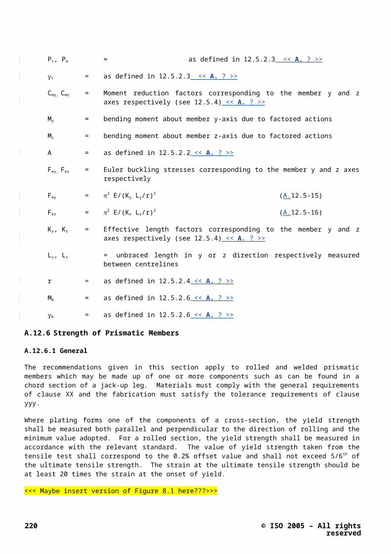
[16] James, R.G. and Tanaka, H. (1984). An investigation of the bearing capacity of footings under eccentric and inclined loading in sand in a geotechnical centrifuge. Proc. Symp. Recent Advances in Geotechnical Centrifuge Modelling, University of California, Davis, pp. 88-115.
[17]Kimura, T., Kusakabe, O. And Saitoh, K. (1985). Geotechnical model tests ofbearing capacity problems in centrifuge, Géotechnique, Vol. 35, No. 1, pp. 33-45.
[18]Martin (2003). New software for rigorous bearing capacity calculations. Proc. British Geotechnical Association Int. Conf. on Foundations, Dundee, UK, pp. 581-592.
[19]Martin (2004). Calculations using Martin’s ABC program (Martin, 2003) and published in Randolph et al., 2004.
[20]Randolph, M.F., Jamiolkowski, M.B. and Zdravkovi, L. (2004). Load carrying capacity of foundations. Proc. Skempton Memorial Conf., London, 1, 207-240.
© ISO 2005 – All rights reserved 225

Bibliography
<< The Bibliography has to be the last section in the whole Part of the Standard >>
1 Bibliography for Clause xx
2 Bibliography for Clause yy
3 Bibliography for Clause zz
4 Bibliography for Clause A.xx
5 Bibliography for Clause A.yy
6 Bibliography for Clause A.zz
7 Bibliography for Clause C
8 Bibliography for Clause D
226 © ISO 2005 – All rights reserved


![[4063] – 67 - Savitribai Phule Pune · PDF file[4063] – 67 T.E. (E & TC/Electronics, ... A step down DC chopper has a resistive load of R=15Ω and input voltage ... thickness of](https://img.dokumen.tips/doc/110x75/5a9dd2c37f8b9abd0a8d9823/4063-67-savitribai-phule-pune-4063-67-te-e-tcelectronics-a.jpg)