DEPARTMENT OF ECONOMICS

ISSN 1441-5429

DISCUSSION PAPER 03/16

Is there a conditional convergence in the per capita incomes of

BIMAROU states in India?

Ankita Mishra1 and Vinod Mishra2*

Abstract: The stochastic income convergence hypothesis is examined for five BIMAROU (Bihar,

Madhya Pradesh, Rajasthan, Orissa and Uttar Pradesh) states in India for the period 1960–2012

using univariate Lagrange multiplier (LM) unit root test that endogenously determines two

structural breaks in level and/or trend of the time series. The per capita incomes of all

BIMAROU states except Uttar Pradesh are found to converge to the national average per capita

income in the long run. Significant structural breaks are detected in relative per capita income

series of BIMAROU states. Most of the breaks spotted in the relative per capita income series

seem to correspond with periods of political uncertainty and regime changes in the state

elections.

Keywords: BIMAROU, Income, Unit Root, Convergence, India

JEL Classification Numbers: O40, C12

1 School of Economics, Finance and Marketing, RMIT University. Email: ankita.mishra@rmit.edu.au 2* Corresponding Author. Department of Economics, Monash University, VIC 3800, Australia.

Email: vinod.mishra@monash.edu. Phone: +61 3 99047179

© 2016 Ankita Mishra and Vinod Mishra

All rights reserved. No part of this paper may be reproduced in any form, or stored in a retrieval system, without the prior

written permission of the author.

monash.edu/ business-economics

ABN 12 377 614 012 CRICOS Provider No. 00008C

1. Introduction

Economic growth models based on New Growth Theory postulate that economies grow when the

capital per hour worked increases and technological improvements take place. As the payoffs from

using additional capital or better technology are greater for poorer economies, such economies should

be able to increase their growth rate at a faster rate than richer economies, thus enabling them to catch

up. Various studies in the literature have taken an empirical view as to whether catch up or

convergence has actually occurred for different groups of countries (Mankiw et al., 1992; Evans,

1996, 1997) and for diverse regions within a single large country. The latter is defined as ‘regional

convergence’, and has been investigated in numerous studies in the literature for various industrial

and emerging market economies (see Young et al., 2008; Carlino & Mills, 1993 for the United States;

Canova & Marcet 1995 for regions in Western Europe; Jian, Sachs, & Warner, 1996, and Weeks &

Yao, 2003 for provinces in China; Koo, Kim, & Kim, 1998 for 10 states in Korea; Ferreira, 1999 for

Brazil; Elias, & Fuentes, 1998 for Chile and Argentina; and de la Fuente, 2002 for regions in Spain).

In this article, we analyse the issue of regional convergence for five of the poorest Indian states,

namely Bihar, Madhya Pradesh, Rajasthan, Uttar Pradesh and Orissa.

In the early 1980s, demographer Ashish Bose examined selected demographic indicators for Indian

states and found that Bihar, Madhya Pradesh, Rajasthan and Uttar Pradesh, which accounted for

nearly 40% population of the country in 1981, very much lagged behind other states on those

indicators. Given the poor demographic performance of these states, Bose coined the acronym

BIMARU, formed from the first letters of the names of these states (i.e. BI: Bihar; MA: Madhya

Pradesh; R: Rajasthan; U: Uttar Pradesh). As the word ‘BIMARU’ resembles a Hindi word ‘BIMAR’

which means ‘sick’, Bose formulated the term to draw the attention of policymakers to the need to

bridge the gap between the demographically ‘sick’ states that comprise BIMARU and the better-

performing states of Kerala, Tamil Nadu, Andhra Pradesh and Karnataka. On this, Bose cautioned

that if the gap was not bridged, it may “cause social turbulence and may even pose a threat to political

stability” (Sharma, 2015). Although the term BIMARU was originally used by Bose to indicate the

poor performance of these states on demographic indicators, the acronym was soon used to refer to

the economic backwardness of these states as well. Later, some scholars expanded BIMARU to

BIMAROU (i.e. BI: Bihar; MA: Madhya Pradesh; R: Rajasthan; O: Orissa; U: Uttar Pradesh) to

include Orissa as well.

Although for many years BIMAROU states were held responsible for dragging down the GDP growth

of India, some recent research suggests otherwise. Ahluwalia (2000), for example, contends that the

so-called characterization of BIMAROU states as a homogeneous group of poor economic performers

does not hold, particularly in the post-reform period 1991–1992 onwards. While many articles in

newspapers and popular media have noted that BIMAROU states are no longer sick because of their

high economic growth rates in the post reform period (Sharma, 2015), there is no consensus on this

subject. For example, Bhattacharya and Sakthivel (2004), and Kumar (2004) assert that the reforms of

the 1990s widened the gap between the richer and poorer states. Purfield (2006) also suggests that the

benefits of growth have remained concentrated in India’s richer states (i.e. Tamil Nadu, Gujarat,

Haryana, Maharashtra and Punjab), leaving the poorer states of India (mainly the BIMAROU states

and some small north-eastern states) further and further behind. Given these conflicting findings on

convergence for BIMAROU states, this paper revisits this issue by employing a time series approach

based on the notion of stochastic convergence, with our empirical findings supporting stochastic

convergence for all BIMAROU states except Uttar Pradesh.

A number of studies have examined the regional convergence hypothesis for per capita income of

Indian states in a very general context, with the majority of these studies adopting a cross-sectional

growth convergence equation approach. Very few studies, however, have used time series stochastic

convergence to examine the income convergence hypothesis for Indian states1. This stochastic

convergence approach is generally based on unit root tests, and is often criticized for low power and

unreliable results due to its ignoring the possibility of structural breaks in the time-series framework

(Ghosh, 2013). Taking into account this criticism, this paper tests stochastic income convergence

hypothesis for BIMAROU states of India for the period 1960–2012 using Lagrange Multiplier (LM)

unit root test that allows for two structural breaks in level and/or trend of the series. This paper

contributes to the literature in two significant ways. First, the testing methodology as used here is not

prone to rejection of the null in the presence of a unit root with break(s), which is a well-documented

criticism aimed at traditional univariate unit root tests such as the Augmented Dickey Fuller (ADF)

and PP tests. In addition, with this approach, the rejection of the null hypothesis (of a unit root)

unambiguously implies stationarity in contrast to earlier uses of unit root tests with breaks, in which

rejection of the null may indicate a unit root with break(s) rather than a stationary series with break(s).

Second, the detection of these structural breaks carries significant implications for policy makers as

state-specific conditioning variables such as physical infrastructure/investment expenditure (as

measured by irrigation, electrification and railway track-building expenditure in Bandyopadhyay

(2011), and Baddeley et al. (2006)), and social infrastructure (defined as human capital in Lahiri et al.

(2009)), can be permanently altered following a major shock and impose permanent changes on the

time path of relative income. While this paper explores whether identified structural breaks can be

linked to significant political, economic and environmental events that occurred around the same time

in a particular state, it does not, however, attempt to establish any causal relationship between such

events and statistically significant breaks in income. The suggested events can only be taken as a

1Refer to Mishra and Mishra (2015) for a list of such studies, their approaches and main results.

likely cause of the structural breaks due to the close associations between the timing of the breaks and

occurrence of the events.

The rest of the paper is organized as follows. Section 2 outlines the econometric methodology;

Section 3 describes the data and some trends observed during preliminary analysis; sections 4 and 5

present the results and discuss the location of structural breaks identified in the per capita income

series; and Section 6 concludes the paper.

2. Econometric methodology

Conventional Unit Root Tests

As a starting point, this paper uses conventional univariate unit root testing methods without structural

breaks. The rationale behind applying these three conventional tests is to use them as a benchmark

against which to compare the respective test versions that include structural breaks. Comparison

between these two sets of results, then, helps to identify the extent to which misspecification is due to

ignoring structural breaks.

The conventional univariate unit root tests that we employ are the ADF (Dickey & Fuller, 1979), the

KPSS stationarity test (Kwiatkowski, Phillips, Schmidt, & Shin, 1992), and the Lagrange multiplier

(LM) unit root test (Schmidt & Phillips, 1992). The null hypothesis for the ADF and the LM unit root

tests is that the relative (to the national average) per capita income series of state 𝑖 contains a unit

root. If the null of a unit root is accepted for the per capita income series of state 𝑖, this implies that

shocks to the income of state 𝑖 relative to the average income (measured by per capita income at the

national level) will be permanent. Hence, the per capita income of state 𝑖 will diverge from national

per capita income. On the contrary, if the null hypothesis of a unit root in the per capita income series

of state 𝑖 is rejected, this suggests that shocks to the income of state 𝑖 relative to national per capita

income will be temporary. Over the long term, the per capita income of state 𝑖 will converge to the

average national per capita income. The KPSS test differs from the ADF and LM unit root tests,

however, in that it has a null hypothesis of stationarity against the alternative hypothesis of unit root.

As these tests are well documented in the literature, we do not discuss their full scope, methodology

and limitations here2.

Unit root tests with two structural breaks

2 For details, refer to Smyth, Nielsen, and Mishra (2009).

The potential problem with conventional unit root tests is that these tests do not take into account the

possibility of structural breaks in data series. As a result, the ability of these tests to reject the null

hypothesis of unit root declines where data series contain structural breaks (Perron, 1989). Many

significant events occurred in the Indian economy in general and BIMAROU states in particular

during the period 1960‒2012, giving rise to the possibility of breaks in the intercept or trend, or both,

of the per capita income of BIMAROU states. Hence, ignoring the possibility of these structural

breaks in the income series of BIMAROU states can lead to misspecification bias and consequently to

misleading conclusions.

This paper uses Lee and Strazicich’s (2003) LM unit root test with two endogenous breaks. The LM

test has the advantage over ADF-type endogenous break tests (Zivot & Andrews, 1992; Lumsdaine &

Papell, 1997) in that it is unaffected by breaks under the null of a unit root. In ADF-type endogenous

break unit root tests, the critical values are derived assuming no break(s) under the null. As a result, in

ADF-type endogenous break unit root tests, rejection of the null may indicate a unit root with break(s)

rather than a stationary series with break(s), giving rise to the spurious rejection problem (Smyth,

Nielsen, & Mishra, 2009). With LM unit root test approach, the rejection of the null hypothesis (of a

unit root) unambiguously implies stationarity.

Lee and Strazicich (2003) developed two versions of the LM unit root test with two structural breaks.

This paper applies the Model CC specification, which can accommodate two breaks in the intercept

and the slope3. The test relies on determining the breaks where the endogenous two-break LM t-test

statistic is at a minimum. Critical values for this case are tabulated in Lee and Strazicich (2003).

3. Data

We use per capita net state domestic product (NSDP) of Bihar, Madhya Pradesh, Rajasthan, Orissa

and Uttar Pradesh for the analysis. The data is collected from Indiastat database. The NSPDs for the

five BIMAROU states were originally expressed in Indian Rupees (INRs) and provided at different

base periods. Hence, all the series are converted to the common base period of 2004‒20054.

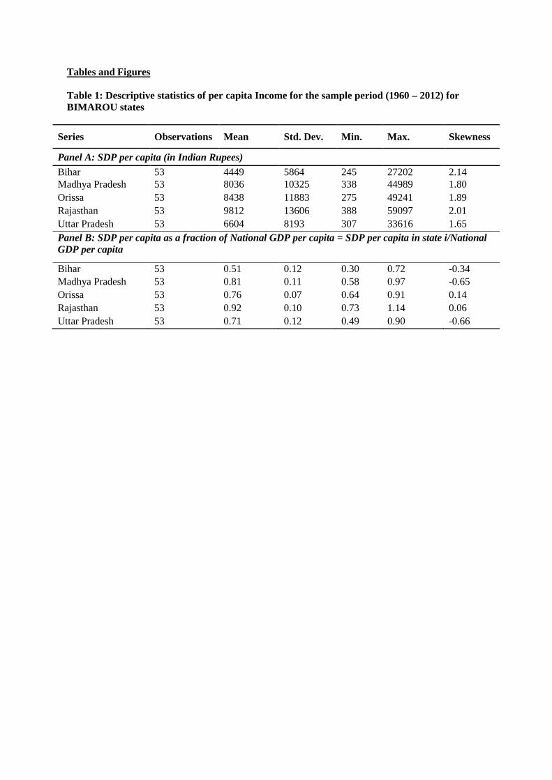
Descriptive statistics on NSDP per capita are reported for the full sample period in Table 1. We note

that among BIMAROU states, Rajasthan has the highest average per capita NSDP while Bihar has the

lowest for the full sample period of 1960–2012. NSDP per capita series for all the states are positively

skewed, which indicates that the future values of NSDP per capita are more likely to be higher than

the mean.

3 For other versions and more technical details of the test, refer to Smyth, Nielsen, and Mishra (2009). 4 The latest base period used for compiling the net state domestic products.

This paper has taken the relative per capita income measure to examine the convergence hypothesis.

For this, the NSDP per capita of state 𝑖 is converted to its relative NSDP per capita in the following

way:

𝑅𝑒𝑙𝑎𝑡𝑖𝑣𝑒 𝑃𝑒𝑟 𝐶𝑎𝑝𝑖𝑡𝑎 𝑁𝑆𝐷𝑃𝑖𝑡 = 𝑙𝑛 (𝑃𝑒𝑟𝐶𝑎𝑝𝑖𝑡𝑎 𝑁𝑆𝐷𝑃𝑖𝑡

𝑁𝑎𝑡𝑖𝑜𝑛𝑎𝑙 𝑃𝑒𝑟 𝐶𝑎𝑝𝑖𝑡𝑎 𝐼𝑛𝑐𝑜𝑚𝑒𝑡)

Panel B of Table 1 presents the descriptive statistics of the relative series of per capita income of state

i/national per capita income. In a hypothetical scenario, where the per capita income of a state is

exactly equal to the national per capita income, this series will take a value of one, whereas a value

smaller than one means that the per capita income of that state is lower, and a value greater than one

indicates that the per capita income of the state is higher than the national average. As expected, the

relative per capita income of BIMAROU states is lower than the national average with Rajasthan

closest to the national average and Bihar farthest.

INSERT TABLE 1 HERE

Trends in per capita income of BIMAROU states

Before undertaking econometric testing to examine convergence for BIMAROU states, we investigate

the trends in income series over the sample period. For this, we divide our sample period into three

sub-periods: 1960–1990 classified as pre-reform period; 1991–1999 classified as reform period; and

2000–2012 classified as post-reform period, such that reforms refer to the 1991 economic

liberalisation of the Indian economy. Panels A and B of Table 2 present the per capita income as a

fraction of national income for BIMAROU states for the three sub-periods. It is evident from Panel B

of Table 2 that over the years the gaps between per capita incomes of BIMAROU states and the

national average have widened in levels. When we look at the growth rates of per capita income for

BIMAROU states in Table 3, we note that growth rate in Rajasthan consistently increased while

growth rate in Madhya Pradesh consistently decreased from one sub-period to the other. For Uttar

Pradesh and Orissa, growth rate increased from 1960–1990 to 1991–1999 but then decreased in 2000–

2012. Bihar registered the highest growth rate in the post-reform period among all the BIMAROU

states. This preliminary investigation of data seems to support the findings of some researchers who

contend that economic reforms favour the richer states of India, leaving the poorer states behind

(Purfield, 2006).

INSERT TABLE 2 HERE

As the notion of convergence suggests, for poorer regions to catch up with the national average, such

regions should grow at a rate higher than the national average. Based on this notion, if we consider the

average growth rate for the full sample period (column 5 of Table 3), Orissa and Rajasthan have

growth rates higher than the national average and seem to catch up, while Bihar, Madhya Pradesh and

Uttar Pradesh have slower growth rates than the national average and seem to be diverging from the

national average in the long run. Based on this preliminary investigation, in the next section we apply

the more rigorous econometric testing procedure to analyse this issue of convergence of BIMAROU

states.

INSERT TABLE 3 HERE

4. Results

As a benchmarking exercise, the ADF and LM unit root tests and the KPSS stationarity test without

structural breaks were carried out for relative per capita income series of BIMAROU states. The

results for these tests are reported in Table 4. The results for the ADF test suggest that the null of unit

root cannot be rejected in any of the relative per capita income series at the traditional levels of

significance. This test gives no evidence of convergence in per capita incomes of BIMAROU states to

the national average. In the KPSS test, the null of stationarity is rejected for 3 of the 5 states. The LM

test fails to reject null of unit root in 4 of the 5 cases. The overall conclusion, which seems evident

based on these tests results, is that there is no convergence in per capita incomes of BIMAROU states

to the national average.

INSERT TABLE 4 HERE

Table 5 presents the LM unit root test results with two endogenous breaks in the intercept and/or

slope. The Lee and Strazicich (2003) LM unit root test has a null hypothesis of unit root in the series.

Model CC, the most general specification of the test, is used here as it allows for two breaks in the

intercept and/or trend of the series. In this test, the null hypothesis of a unit root is rejected (or

accepted) by looking at the LM statistics, and the presence of significant structural breaks are

determined by looking at the significance of the dummies for breaks in intercept and trend. The full

results of this test (including the LM test statistics, the coefficients, and the significance of dummies

for breaks in trend and intercepts for the break dates that were endogenously determined by the test)

are reported in Table 5. The null of a unit root in the relative per capita income series is rejected for

all BIMAROU states except Uttar Pradesh. The results of this test provide evidence in support of the

convergence hypothesis. Looking at the break dates uncovered by the test and the significance of

dummies at those break dates, we observe the following: for Bihar, on the first break date in 1985

there is a break only in trend, while at the second break date in 2001, there is a break in both intercept

as well as trend of the series; for Madhya Pradesh, on the first break date in 1987, none of the

dummies are significant, which suggests the break is not powerful enough to change the level and/or

trend of the series, while a second break in 2004 causes a change in both level and trend of the series;

for Orissa, both the break dates (in 1979 and 2002) change the intercept of the series without affecting

its trend; for Rajasthan, the first break (in 1978) shifts the level while the second break (in 1999)

changes the trend; and for Uttar Pradesh, only the second break (in 2004) seems strong enough to

cause change both in the level as well as trend of the series.

Comparing these results with the results of Table 4 (more specifically, comparing them with the LM

unit root test without structural breaks), we note that the number of states for which the null of unit

root can be rejected increases dramatically to 4 out of 5 compared to 1 out of 5 after allowing for the

structural breaks in the series. Given the conflicting stationarity and non-stationarity results from

different tests, we take the result obtained from the model with structural breaks as the final result.

Tests that allow for structural breaks assume more parameters in the data generating process and

hence provide a better fit to the data. Also, given the time series of the last five decades, it seems

natural to rely on the model with structural breaks. This conclusion is supported by the fact that the

break dates in these states match major socio-political events. In the next section, we discuss the

location of break dates and the events to which they may possibly correspond.

INSERT TABLE 5 HERE

5. Structural Breaks

The presence of structural breaks carries significant implications for our findings as the time path of

relative income can be permanently changed after a major shock. In this section, we analyse the

association between the suggested break dates and any major political or economic event as the

probable cause of the break in the time path of relative per capita incomes of the BIMAROU states.

We observe that for all states except Uttar Pradesh, the first structural break in the series occurs in the

period 1978–1987 while the second structural break for all the states occurs in the period 1999–2004.

It is noted that the Indian economy suffered a macroeconomic crisis in 1979–1980 and again in 1991,

with both crises primarily related to balance of payment. While, the crisis of 1979–1980 was mainly

the result of external factors such as the international oil crises of 1973 and 1979, the crisis of 1991

was due to the unsustainable level of government spending and expenditure on subsidies in the 1980s

that resulted in mounting internal and external debt. In the aftermath of the 1991 crisis, India adopted

a major program of structural and economic reforms.

Table 6 lists the identified structural breaks and the most likely causes of these events for each of the

five BIMAROU states. In the following paragraphs, we discuss these major events in detail and

analyse the effect of these shocks on the overall time path of the relative income of that state.

INSERT TABLE 6 HERE

5.1 Structural breaks in relative income of Bihar

Bihar is located in eastern India and the country’s third largest state by population5. Figure 1 presents

the location of breaks and corresponding trend in its relative per capita income series. We note that

the first break in relative per capita income of Bihar take place in 1984, which seems to correspond to

the turbulent socio-political situation prevailing in India in that year. Violent anti-Sikh riots erupted in

India following the assassination of then Prime Minister Mrs Indira Gandhi by her two Sikh

bodyguards on October 31, 1984, and although these riots originally broke out in Delhi, many

northern states were affected, including Bihar. The Indian National Congress (the political party to

which Mrs Indira Gandhi belonged) ruled Bihar at that time and some of its members being held

responsible for spreading the anti-Sikh riots of 1984. After the first break, the relative per capita

income of Bihar began to fall. In 1990, the governance of the state shifted from the Indian National

Congress, which had ruled the state for most of the years since the country’s independence in 1947, to

the political party Rashtriya Janata Dal (RJD) with Mr Lalu Prasad Yadav in the role of chief minister

of Bihar from 1990–1997. His wife, Mrs Rabri Devi, then served as chief minister from 1997–2005

with a few periods of interruptions. This period from 1990–2005 is characterized as the Lalu

Prasad/Rabri Devi era6 and marked by a complete collapse of the Bihar economy, excessive rise in

crimes and mass outward migration from Bihar to other states. The fallout of both national and

internal factors, then, was that the relative income of Bihar, which in 1984 had been 0.59 of the

national average, dwindled to 0.30 in 2005. The second break in the income series of Bihar occurred

in 2001. The two most likely events that led to the break around this time were the formation of the

new state Jharkhand out of Bihar in 2000, as well as the change in political regime from Lalu

Prasad/Rabri Devi to Mr Nitish Kumar of Janata Dal (United), who became chief minister in 2005. As

Figure 1 shows, per capita income in Bihar has revived since then, with Nitish Kumar initiating

various social and infrastructure development projects in Bihar that resuscitated economic growth. As

a result, the per capita income in Bihar grew roughly at the rate of 19% per year from 2005–2012,

which was markedly higher than the national average of 14%.

5 This information is taken from Bihar Government’s official website www.bihar.gov.in 6 Rashtriya Janata Dal (RJD) is a political party formed by Mr Lalu Prasad Yadav in 1997 after he was expelled

from Janata Dal (the party to which Mr Lalu Yadav earlier belonged) on corruption charges.

INSERT FIGURE 1 HERE

5.2 Structural breaks in relative income of Madhya Pradesh

Madhya Pradesh is a resource rich state with India’s largest reserves of copper and diamonds as well

as various other mineral reserves, including coal. Figure 2 presents the location of breaks and

corresponding trend in its relative per capita income series. We note that the first break in relative per

capita income of Madhya Pradesh occurred in 1987. The most likely cause of this break appears to be

the Bhopal Gas Tragedy of 1984, which took place in Madhya Pradesh’s capital city of Bhopal. On

December 3, 1984, a chemicals manufacturing company (Union Carbide Corporation) released

methyl isocyanate (MIC) into the atmosphere above Bhopal. The leak was attributed to employer

negligence and poor plant maintenance, with the state government officially placing the death toll at

around 4,000. However, unofficial estimates claim that it killed 20,000 and injured over 500,000

people, making it the world’s worst industrial disaster. To compound the tragedy of lost lives and

injuries, the gas leak also impacted economic growth in Madhya Pradesh by adversely affecting

transportation and supply of other necessities as well as the working ability of 75% of Bhopali

citizens7. These factors affected the growth in per capita income of Madhya Pradesh in the 1980s,

with its average per capita income growing roughly 4 times from one break date to another (1987-

2004) while during the same period the average national per capita income grew 6 times. The second

break in the relative per capita income of Madhya Pradesh is detected in 2004. The two most likely

events leading to this break appear to be the formation of the new state Chattisgarh out of Madhya

Pradesh, and the shift in Madhya Pradesh’s political regime in 2003 to the Bhartiya Janata Party (BJP)

after the state’s being mainly governed by the Indian National Congress since 1947. After the second

break, the per capita income in Madhya Pradesh grew roughly 3 times which was almost the same

(marginally higher) as the national average of 2.8 times.

INSERT FIGURE 2 HERE

5.3 Structural breaks in relative income of Orissa

The state of Orissa has a large coastline and is enriched with abundant natural resources. Figure 3

presents the location of breaks and corresponding trend in its relative per capita income series. The

first break in relative per capita income series of Orissa is detected in 1979. The most significant

corresponding event is the establishment in 1981 of NALCO (National Aluminium Company

Limited), which is one of Asia’s largest integrated aluminium complexes with headquarters in

Bhubaneswar, the capital city of Orissa. Although a big infrastructure project such as NALCO

contributes to productivity and production, it also causes undesirable effects including deforestation,

7 Taken from Source: http://bhopalgasdisaster.weebly.com/economic-effects.html

loss of agricultural land, environmental degradation and marginalization of the weaker sections

(Mohanty, 2011). As noted by Mohanty, while the beneficial ‘spread effects’ of a project like

NALCO are enjoyed by the nation as a large, its adverse effects mainly impact the local population.

Notwithstanding these various contradictory effects, we find an improvement in the relative per capita

income of Orissa for the first few years after NALCO’s establishment in 1981. However, from this

time until the next break in relative income in 1999, Orissa’s relative income as a fraction of national

average fell from 0.85 to 0.69. The next break in relative per capita income of Orissa is spotted in

2002. The most likely cause of this break seems to be the cyclone of 1999 that caused huge economic

damage and loss of human lives. In the aftermath of this cyclone, from 1999–2002 the growth rate in

per capita income of Orissa fell below the national average. Post-2002, however, per capita income

growth started to pick up, and from 2002— 2012 the per capita income of Orissa grew 3.9 times

against the national average of 3.5 times.

INSERT FIGURE 3 HERE

5.4 Structural breaks in relative income of Rajasthan

While Rajasthan is the largest state of India in terms of area, a large portion is desert with little forest

cover. Figure 5 presents the location of breaks and corresponding trend in its relative per capita

income series. The first break in the relative per capita income series of Rajasthan is spotted in 1978.

The most likely cause of this break is the political uncertainty prevailing in Rajasthan from 1977–

1980 before the Indian National Congress came to power in June 1980, where it remained until 1990.

During this time of stability, per capita income of Rajasthan grew 3.4 times which was slightly better

than the national average of 3.04 times. In 1990, power shifted from the Congress party to the

Bhartiya Janata Party (BJP), which governed the state till 1998 with a brief period of president’s rule.

From 1990–1998, the per capita income of Rajasthan grew 2.5 times which was slightly lower than

the national average of 2.6 times. In 1998, power again shifted from BJP to the Congress party and

roughly around this time we spot the second break in Rajasthan’s relative per capita income series.

Relative per capita income of Rajasthan began to show signs of improvement and also better

performance than the national level around 2009. However, the post-2009 sample is not long enough

to detect any decisive trend in per capita income.

INSERT FIGURE 4 HERE

5.5 Structural breaks in relative income of Uttar Pradesh

Uttar Pradesh is the most populous and one of the poorest states of India. Figure 5 depicts the breaks

in the relative per capita series for Uttar Pradesh. The first structural break in the relative income

series of Uttar Pradesh is noted in 1992. The most likely cause of this break seems to be the

demolition of a disputed Mosque-like structure in Ayodhaya (a city in the Faizabad district of Uttar

Pradesh) in 1992, and the consequent outbreak of Hindu-Muslim riots in Uttar Pradesh and in many

other parts of India that resulted in an estimated death toll of more than 2,000 people. The 16-year

period from 1991–2007 was a time of major political uncertainty for Uttar Pradesh. From the

beginning of the government led by Mr Mualayam Singh in December 1989 and the start of the

government led by Ms Mayawati in May 2007, the state witnessed 14 changes of government

(accompanied by extended periods of president’s rule), with no chief minister completing his/her full

term. The average per capita income in India increased around 5.5 times between 1991 and 2007

while the per capita income in Uttar Pradesh increased only 3.5 times. In terms of relative per capita

income, Uttar Pradesh actually became poorer compared with the rest of India. In 1991, the relative

per capita SDP of Uttar Pradesh was 77% of national per capita income, falling to 50% a decade and a

half later in 2007. Another structural break in Uttar Pradesh’s data series occurred in 2007 at the same

time as the Mayawati government was elected. The Mayawati Government became the first

government to complete its full term of five years after a period of 16 years. However, the post-2007

sample is too small to be conclusive about the trend in relative per capita income series since that

year.

INSERT FIGURE 5 HERE

6. Conclusion

This paper examines the stochastic income convergence hypothesis for five BIMAROU states in India

using relative per capita income series from 1960–2012. To test this hypothesis we employ univariate

Lagrange multiplier (LM) unit root test that endogenously determines two structural breaks either in

level and/or trend of the time series. With this approach, the rejection of the null hypothesis (of a unit

root) unambiguously implies stationarity in contrast to earlier uses of unit root tests with breaks, in

which rejection of the null may indicate a unit root with break(s) rather than a stationary series with

break(s). After controlling for breaks, we find that the relative incomes of BMAROU states are

conditionally converging to the national average with the exception of Uttar Pradesh. The main reason

for the diverging per capita income of Uttar Pradesh appears to be lack of coherent economic policies

due to frequent changes in government in the period 1990–2007. The political instability that

prevailed in the state for most of the previous two decades seems to have permanently altered the

growth path of relative per capita income series of Uttar Pradesh.

References

Ahluwalia, M. S. (2000). Economic performance of states in post-reforms period. Economic and

Political Weekly, 35(19)

Baddeley, M., McNay, K., and Cassen, R. (2006). Divergence in India: Income differentials at the

state level, 1970–97. Journal of Development Studies, 42(6), 1000–1022.

Bhattacharya, B. B., and Sakthivel, S. (2004). Regional growth and disparity in India: Comparison of

pre- and post-reform decades. Economic and Political Weekly, 39(10), 1071–1077.

Bandyopadhyay, S. (2011). Rich states, poor states: Convergence and polarisation in India. Scottish

Journal of Political Economy, 58(3), 414–436.

Canova, F. and Marcet, A. (1995). The poor stay poor: Non-Convergence across

countries and regions. Universitat Pompeu Fabra Economics Working Paper No. 137 (Barcelona).

Carlino, G. A., & Mills, L. O. (1993). Are U.S. regional incomes converging? Journal of Monetary

Economics, 32(2), 335–346

De la Fuente, A. (2002). Regional Convergence in Spain, 1965–95. CEPR Discussion

Papers, No. 3137 (London: Center for Economic Policy Research).

Dickey, D. A., and Fuller, W. A. (1979). Distribution of the estimators for autoregressive time series

with a unit root. Journal of the American Statistical Association, 74, 427–431.

Elias, V.J., and Fuentes, R. (1998). Convergence in the Southern cone. Estudios de

Economia, 25(2) 179–89

Evans, P. (1996). Using cross-country variances to evaluate growth theories. Journal of Economic

Dynamics and Control, 20(6), 1027–1049.

Evans, P. (1997). How fast do economics converge? Review of Economics and Statistics, 79(2), 219–

225.

Ferreira, A. H. B. (1999). Concentração regional e dispersãp das renas per capita estaduais: Um

comentário. Estudias Economicãs, 29(10), 47–63

Ghosh, M. (2013). Regional economic growth and inequality. In liberalization, growth and regional

disparities in India. India Studies in Business and Economics series 17–45, Springer India.

doi:10.1007/978-81-322-0981-2_3

Jian, T., Sachs, J. and Warner, A. (1996). Trends in regional inequality in China. NBER Working

Paper Series, No. 5412 (Cambridge, Massachusetts:National Bureau of Economic Research).

Koo, J., Kim, Y.Y. and Kim, S. (1998). Regional income convergence: Evidence from a rapidly

growing economy. Journal of Economic Development, 23(2), 191–203.

Kumar, S. (2004). Impact of economic reforms on the Indian electorate. Economic and Political

Weekly, 39(16), 1621–1630

Kwiatkowski, D., Phillips, P. C. B., Schmidt, P., and Shin, Y. (1992). Testing the null hypothesis of

stationarity against the alternative of a unit root: How sure are we that economic time series have a

unit root? Journal of Econometrics, 54(1), 159–178.

Lahiri, A. and Yi, K.-M. (2009). A tale of two states: Maharashtra and West Bengal. Review of

Economic Dynamics, 12 (3), 523–542.

Lee, J., and Strazicich, M. C. (2003). Minimum Lagrange multiplier unit root test with two structural

breaks. Review of Economics and Statistics, 85(4), 1082–1089.

Lumsdaine, R. L., and Papell, D. H. (1997). Multiple trend breaks and the unit-root hypothesis.

Review of Economics and Statistics, 79, 212–218.

Mankiw, N., Romer, D., & Weil, D. (1992). A contribution to the empirics of economic growth.

Quarterly Journal of Economics, 107(2), 407-438

Mishra, A. and Mishra, V. (2015). Examining income convergence among Indian states: Time series

evidence with structural breaks. Monash Business School, Department of Economics Discussion

Paper No. 44/15

Mohanty, R. (2011). Impact of development project on the displaced tribals: A case study of a

development project in eastern India. Orissa Review September-October 2011

Perron, P. (1989). The great crash, the oil price shock and the unit root hypothesis, Econometrica, 57,

1361–1401.

Purfield, C. (2006). Mind the gap: Is economic growth in India leaving some states behind? IMF

working paper WP/06/103

Schmidt, P., and Phillips, P. C. B. (1992). LM tests for a unit root in the presence of deterministic

trends. Oxford Bulletin of Economics and Statistics, 54(3), 257–287.

Sharma, V. (2015). Are BIMARU states still Bimaru? Economic and Political Weekly, 50(18), 58–63

Smyth, R., Nielsen, I., and Mishra, V. (2009). I”ve been to Bali too’ (and I will be going back): are

terrorist shocks to Bali’s tourist arrivals permanent or transitory? Applied Economics, 41(11), 1367–

1378.

Weeks, M. and Yao, J. Y. (2003). Provincial conditional income convergence in China, 1953–1997:

A Panel data approach. Econometric Review, 22(1), 59–77.

Young, A. T., Higgins, M. J., and Levy, D. (2008). Sigma Convergence versus Beta Convergence:

Evidence from U.S. County-Level Data. Money, Credit and Banking, 40(5), 1083–93

Zivot, E., & Andrews, D. W. K. (1992). Further Evidence on the Great Crash, the Oil-Price Shock,

and the Unit-Root Hypothesis. Journal of Business and Economic Statistics, 10.

Tables and Figures

Table 1: Descriptive statistics of per capita Income for the sample period (1960 – 2012) for

BIMAROU states

Series Observations Mean Std. Dev. Min. Max. Skewness

Panel A: SDP per capita (in Indian Rupees)

Bihar 53 4449 5864 245 27202 2.14

Madhya Pradesh 53 8036 10325 338 44989 1.80

Orissa 53 8438 11883 275 49241 1.89

Rajasthan 53 9812 13606 388 59097 2.01

Uttar Pradesh 53 6604 8193 307 33616 1.65

Panel B: SDP per capita as a fraction of National GDP per capita = SDP per capita in state i/National

GDP per capita

Bihar 53 0.51 0.12 0.30 0.72 -0.34

Madhya Pradesh 53 0.81 0.11 0.58 0.97 -0.65

Orissa 53 0.76 0.07 0.64 0.91 0.14

Rajasthan 53 0.92 0.10 0.73 1.14 0.06

Uttar Pradesh 53 0.71 0.12 0.49 0.90 -0.66

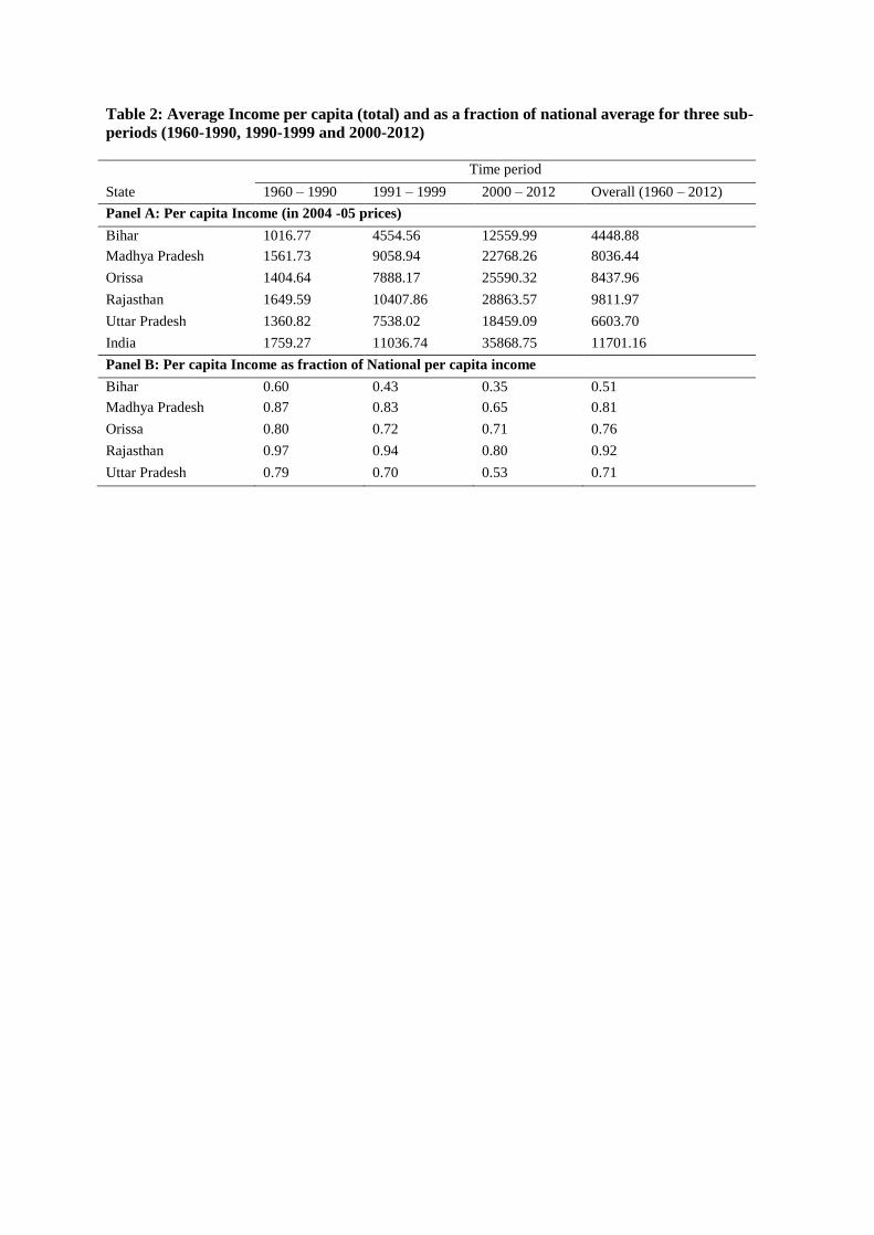
Table 2: Average Income per capita (total) and as a fraction of national average for three sub-

periods (1960-1990, 1990-1999 and 2000-2012)

Time period

State 1960 – 1990 1991 – 1999 2000 – 2012 Overall (1960 – 2012)

Panel A: Per capita Income (in 2004 -05 prices)

Bihar 1016.77 4554.56 12559.99 4448.88

Madhya Pradesh 1561.73 9058.94 22768.26 8036.44

Orissa 1404.64 7888.17 25590.32 8437.96

Rajasthan 1649.59 10407.86 28863.57 9811.97

Uttar Pradesh 1360.82 7538.02 18459.09 6603.70

India 1759.27 11036.74 35868.75 11701.16

Panel B: Per capita Income as fraction of National per capita income

Bihar 0.60 0.43 0.35 0.51

Madhya Pradesh 0.87 0.83 0.65 0.81

Orissa 0.80 0.72 0.71 0.76

Rajasthan 0.97 0.94 0.80 0.92

Uttar Pradesh 0.79 0.70 0.53 0.71

Table 3: Average Income per capita growth rates per year (in percentage terms) for three sub-

periods (1960-1990, 1990-1999 and 2000-2012)

Time period

State 1960 – 1990 1991 – 1999 2000 – 2012 Overall (1960 – 2012)

Bihar 9.00 8.67 12.46 9.81

Madhya Pradesh 10.50 10.49 10.16 10.42

Orissa 9.89 13.16 12.13 11.02

Rajasthan 10.26 11.49 11.57 10.80

Uttar Pradesh 9.58 10.11 9.58 9.67

India 9.61 12.49 11.53 10.59

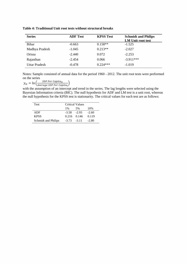
Table 4: Traditional Unit root tests without structural breaks

Series ADF Test KPSS Test Schmidt and Philips

LM Unit root test Bihar -0.663 0.158** -1.525

Madhya Pradesh -1.045 0.213** -2.027

Orissa -2.440 0.072 -2.253

Rajasthan -2.454 0.066 -3.911***

Uttar Pradesh -0.478 0.224*** -1.019

Notes: Sample consisted of annual data for the period 1960 - 2012. The unit root tests were preformed

on the series

𝑦𝑖𝑡 = ln (𝑆𝐷𝑃 𝑃𝑒𝑟 𝐶𝑎𝑝𝑖𝑡𝑎𝑖𝑡

𝐴𝑣𝑒𝑟𝑎𝑔𝑒 𝑆𝐷𝑃 𝑃𝑒𝑟 𝐶𝑎𝑝𝑖𝑡𝑎𝑡)

with the assumption of an intercept and trend in the series. The lag lengths were selected using the

Bayesian Information criteria (BIC). The null hypothesis for ADF and LM test is a unit root, whereas

the null hypothesis for the KPSS test is stationarity. The critical values for each test are as follows:

Test Critical Values

1% 5% 10%

ADF -3.58 -2.93 -2.60

KPSS 0.216 0.146 0.119

Schmidt and Philips -3.73 -3.11 -2.80

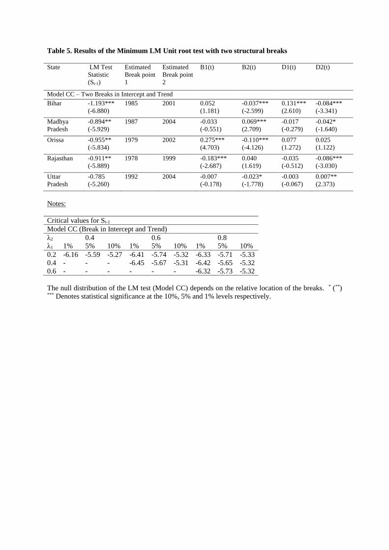
Table 5. Results of the Minimum LM Unit root test with two structural breaks

State LM Test

Statistic

(St-1)

Estimated

Break point

1

Estimated

Break point

2

B1(t) B2(t) D1(t) D2(t)

Model CC – Two Breaks in Intercept and Trend

Bihar -1.193***

(-6.880)

1985 2001 0.052

(1.181)

-0.037***

(-2.599)

0.131***

(2.610)

-0.084***

(-3.341)

Madhya

Pradesh

-0.894**

(-5.929)

1987 2004 -0.033

(-0.551)

0.069***

(2.709)

-0.017

(-0.279)

-0.042*

(-1.640)

Orissa -0.955**

(-5.834)

1979 2002 0.275***

(4.703)

-0.110***

(-4.126)

0.077

(1.272)

0.025

(1.122)

Rajasthan -0.911**

(-5.889)

1978 1999 -0.183***

(-2.687)

0.040

(1.619)

-0.035

(-0.512)

-0.086***

(-3.030)

Uttar

Pradesh

-0.785

(-5.260)

1992 2004 -0.007

(-0.178)

-0.023*

(-1.778)

-0.003

(-0.067)

0.007**

(2.373)

Notes:

Critical values for St-1

Model CC (Break in Intercept and Trend)

λ2 0.4 0.6 0.8

λ1 1% 5% 10% 1% 5% 10% 1% 5% 10%

0.2 -6.16 -5.59 -5.27 -6.41 -5.74 -5.32 -6.33 -5.71 -5.33

0.4 - - - -6.45 -5.67 -5.31 -6.42 -5.65 -5.32

0.6 - - - - - - -6.32 -5.73 -5.32

The null distribution of the LM test (Model CC) depends on the relative location of the breaks. * (**) *** Denotes statistical significance at the 10%, 5% and 1% levels respectively.

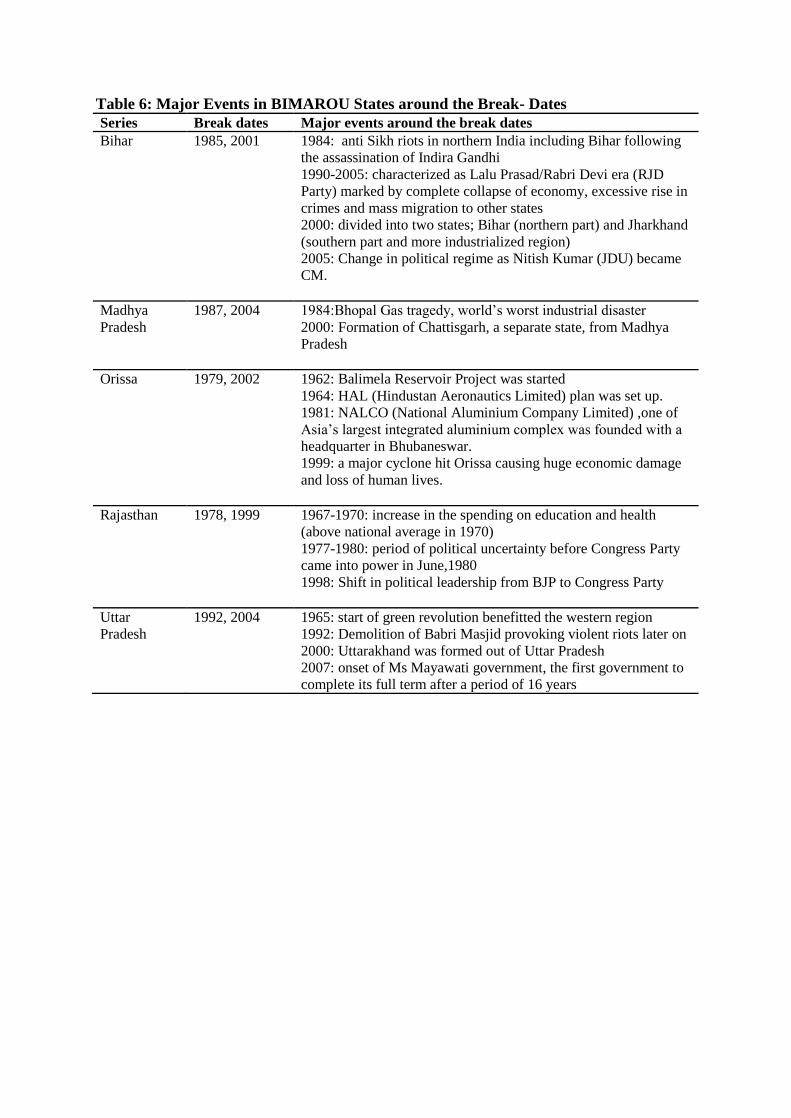
Table 6: Major Events in BIMAROU States around the Break- Dates

Series Break dates Major events around the break dates

Bihar 1985, 2001 1984: anti Sikh riots in northern India including Bihar following

the assassination of Indira Gandhi

1990-2005: characterized as Lalu Prasad/Rabri Devi era (RJD

Party) marked by complete collapse of economy, excessive rise in

crimes and mass migration to other states

2000: divided into two states; Bihar (northern part) and Jharkhand

(southern part and more industrialized region)

2005: Change in political regime as Nitish Kumar (JDU) became

CM.

Madhya

Pradesh

1987, 2004 1984:Bhopal Gas tragedy, world’s worst industrial disaster

2000: Formation of Chattisgarh, a separate state, from Madhya

Pradesh

Orissa 1979, 2002 1962: Balimela Reservoir Project was started

1964: HAL (Hindustan Aeronautics Limited) plan was set up.

1981: NALCO (National Aluminium Company Limited) ,one of

Asia’s largest integrated aluminium complex was founded with a

headquarter in Bhubaneswar.

1999: a major cyclone hit Orissa causing huge economic damage

and loss of human lives.

Rajasthan 1978, 1999 1967-1970: increase in the spending on education and health

(above national average in 1970)

1977-1980: period of political uncertainty before Congress Party

came into power in June,1980

1998: Shift in political leadership from BJP to Congress Party

Uttar

Pradesh

1992, 2004 1965: start of green revolution benefitted the western region

1992: Demolition of Babri Masjid provoking violent riots later on

2000: Uttarakhand was formed out of Uttar Pradesh

2007: onset of Ms Mayawati government, the first government to

complete its full term after a period of 16 years

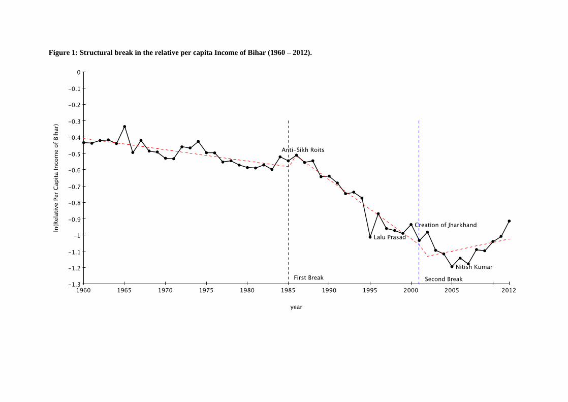
Figure 1: Structural break in the relative per capita Income of Bihar (1960 – 2012).

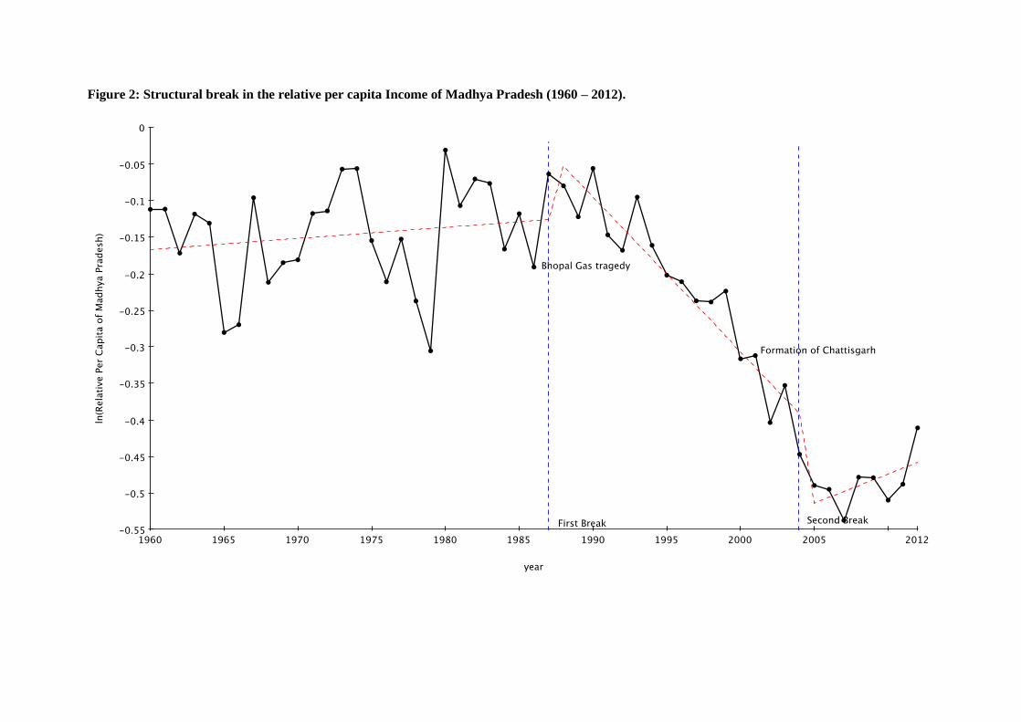
Figure 2: Structural break in the relative per capita Income of Madhya Pradesh (1960 – 2012).

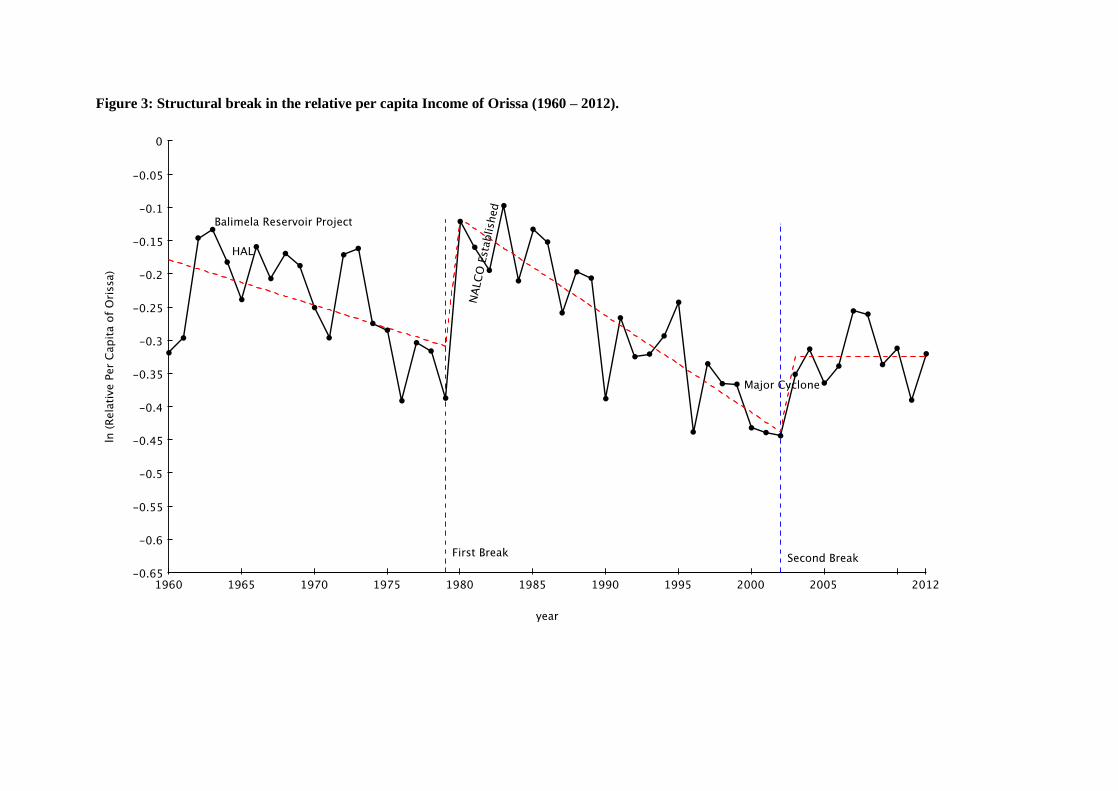
Figure 3: Structural break in the relative per capita Income of Orissa (1960 – 2012).

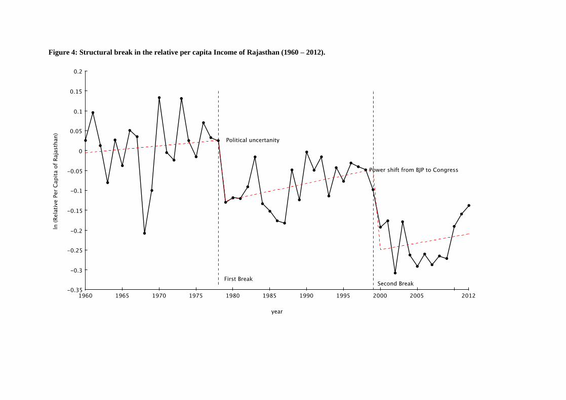
Figure 4: Structural break in the relative per capita Income of Rajasthan (1960 – 2012).

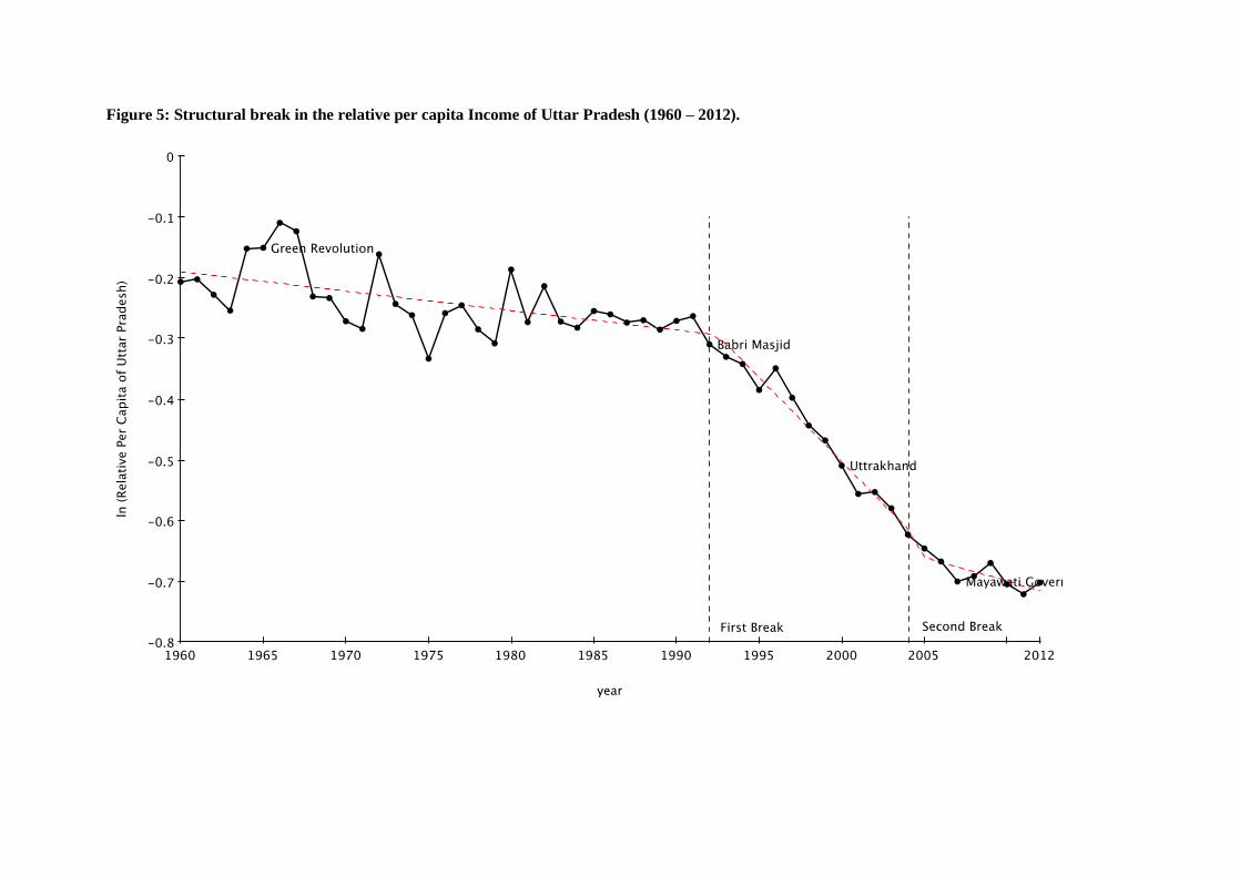
Figure 5: Structural break in the relative per capita Income of Uttar Pradesh (1960 – 2012).