Embed Size (px)
Citation preview

Is Financial Globalization Polluting? – Symmetricand Asymmetric Effects of External Liabilities onCO2 Emissions in the MENA RegionBrahim Gaies
IPAG Business School Paris Campus: IPAG Business SchoolMohamed Sahbi Nakhli
Universite de Kairouan Institut Superieur d'Informatique et de Gestion de Kairouanhttps://orcid.org/0000-0001-5708-5314
Jean-Michel SAHUT ( [email protected] )IDRAC Lyon https://orcid.org/0000-0002-4228-9207
Research Article
Keywords: �nancial globalization, CO2, FDI, portfolio investment, debt, non-linear dynamics
Posted Date: May 24th, 2021
DOI: https://doi.org/10.21203/rs.3.rs-467034/v1
License: This work is licensed under a Creative Commons Attribution 4.0 International License. Read Full License
Is Financial Globalization Polluting? – Symmetric and Asymmetric Effects
of External Liabilities on CO2 Emissions in the MENA Region
Brahim Gaies
IPAG Lab, IPAG Business School, France
Mohamed Sahbi Nakhli
ISIG Kairouan, University of Kairouan, Tunisia
LaREMFIQ Laboratory, University of Sousse, Tunisia
Jean-Michel Sahut (*)
IDRAC Business School, France
Abstract
This paper aims to study the symmetric and asymmetric effects of financial globalization on
CO2 emissions in the MENA region. Using a panel dataset of seven non-OPEC MENA
countries over the period 1980-2014, we perform a comprehensive econometric analysis
based on the panel ARDL and non-linear panel ARDL (NARDL) models and a battery of
tests, including cross-sectional dependence tests, second-generation unit root tests and
cointegration tests. The findings reveal a significant long-term impact of financial
globalization on CO2 emissions that can be symmetric or asymmetric depending on the nature
of financial globalization. While external debt liabilities appear to be polluting because they
increase CO2 emissions significantly and linearly, the long-term impact of FDI and portfolio
investment liabilities on CO2 emissions is asymmetric, with only negative shocks of FDI and
portfolio investment decreasing CO2 emissions. This suggests that financial globalization
through foreign investment (FDI and portfolio investment) is more environmentally friendly
than financial globalization through debt, which provides interesting insights for policy
makers.
Keyword: financial globalization; CO2; FDI; portfolio investment; debt; non-linear dynamics
(*) Correspondence to [email protected]

1. Introduction
Since the Industrial Revolution, CO2 levels have increased by more than 40%1
worldwide. About 7% of the 32 gigatons of carbon dioxide (CO2) emitted each year comes
from the MENA region (World Bank, 2016). However, these emissions are not homogenous
across MENA countries. The major oil producers and members of OPEC (Organization of the
Petroleum Exporting Countries) emit the most CO2, and they have access to this fossil fuel at
a low cost and no or very low taxes on petroleum products. On the contrary, despite the fact
that the non-OPEC MENA countries are relatively less CO2 emitters, they have made very
strong commitments at COP21 (the 2015 UN climate change conference) to reduce their
emissions, as is the case of Tunisia2. This leads the governments of these countries to review
their growth model, taking into account their internal constraints – including high
unemployment rates – and especially external constraints – including the negative trade
balance and the low quality of technological transfer – in an increasingly globalized world.
Thus, rethinking financial openness is essential to reassess the growth model of non-OPEC
MENA countries in light of the link between financial globalization and pollution. Since the
1990s, these countries have opted for greater financial integration allowing foreign capital
flows, particularly foreign direct investment (FDI) and external debt, to increase investment,
consumption, technology transfer, and income, as is the case for many other developing
countries (Hakimi and Hamdi, 2017; Gaies and Nabi, 2019). However, in terms of its effects
on climate, financial globalization appears to be a complex and multifaceted phenomenon,
especially in the MENA region. For the “pessimists”, FDI positively impacts CO2 emissions
and thus increases climate risk (Pethigm, 1976; Walter and Ugelow, 1979; Radermacher,
1994; Omri et al., 2014; Abdouli and Hammami, 2016, Raggad, 2020). This effect is even
stronger in countries with few environmental regulations and many polluting industries, such
as the cement and chemical industries.3 For the “optimists”, the effect of FDI on CO2
emissions is negative (Birdsall and Wheeler, 1993; Al-Mulali and Tang, 2013; Ong and Sek,
2013). From this perspective, the technology transfer achieved by FDI provides access to
new, less polluting technologies and leads to a reduction in CO2 emissions (Liu et al., 2017).
The opposition between these two theses has generated a real debate in the literature, known
as the “pollution haven hypothesis” opposing the “pollution halo hypothesis”. Recently, this led Xie et al. (2020) to study the direct and spillover effects of FDI inflows on CO2 emissions
in emerging countries using a non-linear analysis based on the panel smooth transition
regression (PSTR) model. The authors found that both the pollution haven hypothesis and the
population halo hypothesis are verified under a threshold effect of FDI on CO2. As far as we
know, this is the first study that examines the non-linear relationship between financial
globalization and carbon emissions that integrates the two hypotheses – haven and halo – into
the methodological design. In addition, previous studies on the financial globalization-CO2
emissions nexus appear to have shortcomings in terms of measuring financial globalization in
developing countries. Many authors demonstrate the importance of the three pillars of
financial globalization, which are FDI, debt, and portfolio investment (Estrada et al., 2015;
1 https://www.geospatialworld.net/blogs/managing-the-business-risk-of-climate-change/ 2 https://www.giz.de/en/worldwide/87133.html 3 https://www.bbc.com/news/science-environment-46455844

Ahmed, 2016; Trabelsi and Cherif, 2017) on the economic and financial development.
Although financial globalization is largely dominated by both FDI and debt in developing
countries with increased growth in portfolio investment (Levy-Yeyati and Williams, 2011;
Gaies and Nabi, 2019), it is questionable why almost all empirical studies on the relationship
between financial globalization and CO2 emissions use FDI alone as an indicator to capture
the phenomenon of financial globalization in these countries (Koçak, and Şarkgüneşi, 2018). In order to overcome these two limitations and better understand the relationship between
financial globalization and carbon emissions in non-OPEC MENA countries, this study
develops a comprehensive econometric analysis based on the panel ARDL and non-linear
panel ARDL (NARDL) models and a battery of tests including cross-sectional dependence
tests, second-generation unit root tests, and cointegration tests. This allows to examine the
symmetric and asymmetric effects of financial globalization on CO2 emissions and to
incorporate both the pollution haven and the pollution halo hypotheses in the research design.
To the best of our knowledge, our study is the first attempt to study the financial
globalization-pollution nexus in the MENA region using the panel ARDL and non-linear
panel ARDL (NARDL). Recently, the studies by Raggad (2020) and Boufateh and Saadaoui
(2020) used the NARDL technique to examine the link between macro-finance and carbon
emissions, but they focused on financial development, not financial globalization, and did not
consider the case of MENA countries. This study is also one of the few analyses on the
relationship between financial globalization and CO2 emissions that uses three different
indicators of financial globalization, namely FDI liabilities, portfolio investment liabilities,
and debt liabilities. As mentioned above, previous studies primarily used FDI while ignoring
other types of external liabilities.
Overall, the contribution of this paper is twofold. First, using the ARDL and NARDL
models, it demonstrates that financial globalization can have various and complex impacts on
carbon emissions, thus reconciling the views of “optimists” and “pessimists”. It highlights the asymmetric relationship between financial globalization and CO2 emissions. Second, this
paper shows the relevance of analyzing financial globalization in MENA countries through its
three pillars: FDI, external debt, and portfolio investment. It thus provides a deeper
understanding of the relationship between financial globalization and carbon emission. This is
particularly important for non-OPEC MENA countries, as a better grasp of the complexity of
this link would allow them to review their growth model in light of the global environmental
issue in a context of financial globalization. Moreover, while non-OPEC MENA countries
may not be the most polluting in the MENA region, they already suffer from high
temperatures and water shortages and have little room to adapt given their economic and
financial underdevelopment (Gilmont, 2015).
The remainder of this paper is organized as follows. Section 2 presents a selection of
empirical studies on the relationship between financial globalization and CO2 emissions in
developing countries, particularly in the MENA region. The data, empirical framework, and
results are discussed in section 3. Section 4 explains the autoregressive distributed lag
(ARDL) and the non-linear autoregressive distributed lag (NARDL) models and discusses
their results. Section 5 concludes.

2. Literature review
The literature on the macro determinants of carbon emissions is clearly abundant. In
order to study the impact of financial globalization on CO2 emissions in seven MENA
countries, we focus our review on studies concerning developing countries – including
MENA countries – considering one or more aspects of financial globalization as the
explanatory variable(s) of interest. In doing so, it appears that almost all previous studies have
used FDI inflows as the sole indicator of financial globalization and CO2 emissions as the
indicator of CO2 emissions. It is no secret that FDI inflows have a considerable effect on
GDP growth (e.g., Estrada et al., 2015; Ahmed, 2016; Trabelsi and Cherif, 2017; Gaies et al.,
2020). Beyond economic growth, scholars have also investigated other impacts of FDI
inflows, including on the environment. In this sense, two strands of literature have emerged,
the first pointing towards a positive impact of FDI on CO2 emissions, and thus a harmful
effect on the environment (Abdouli and Hammami, 2016).
2.1 Positive effect of FDI on CO2
This “pessimistic” current finds its origin in the Pollution Haven Hypothesis (PHH)
developed by Pethigm (1976) and Walter and Ugelow (1979). In analyzing the PHH, some
authors point to a link between FDI inflows and CO2 emissions, where the former increase
the latter, particularly in industries with high levels of pollution in countries with few
environmental regulations. In fact, with reference to Abdouli and Hammami (2016) who
examine a sample of developed countries, Shahbaz et al. (2019) explore the PPH in MENA
countries and the increase in industries with high pollution levels, confirming that FDI
generates CO2 emissions. For the Middle Eastern countries Saudi Arabia, Oman and Qatar,
Kari and Sadam (2012) find that the increase in FDI inflows also contributes to increasing per
capita CO2 emissions. Contrary to the assumption that FDI inflows include the replacement
of polluting technologies with less polluting ones (e.g., Gallagher 2004, 2009; Liu et al.,
2017), the authors evidence that for the three countries cited, FDI inflows have not
contributed to more sustainable growth, thus raising CO2 emissions. In the same vein,
Neequaye and Oladi (2015) and Shahbaz et al. (2015) investigate the effect of FDI on CO2
emissions, supporting the PHH for the MENA region. Similar results have been found for
Ghana (Solarin et al., 2017) and Turkey (Koçak and Sarkgünes, 2017). Other authors,
including Lan (2012), Shahbaz et al. (2015), Ouyang and Lin (2015) and Nasir et al. (2019)
also confirm the PPH in the case of developing countries. In addition, besides their direct
effect, FDI inflows may also impact CO2 emissions indirectly via economic growth (Xie et
al., 2019). In fact, on the one hand, FDI and GDP growth are indisputably linked, with FDI
influencing growth, as has been shown in numerous studies (e.g., Estrada et al., 2015; Ahmed,
2016; Trabelsi and Cherif, 2017; Gaies et al., 2020). On the other hand, the existing literature
provides evidence of a direct – equally undisputed – relationship between growth and CO2
emissions (e.g., Sinha et al., 2017; Nabavi-Pelesaraei et al., 2018; Kaab et al., 2019).
2.2 Negative effect of FDI on CO2
The second strand – an “optimistic” one – often invokes the pollution halo hypothesis
developed by Birdsall and Wheeler (1993). This current generally refers to the positive
influence that technology transfer has on reducing CO2 emissions (Xie et al. 2019). Along
these lines, and contrary to the previously mentioned investigations on the PHH, Al-Mulali
and Tang (2013) refute the positive link between FDI and CO2 emissions in host countries. In
fact, by testing the PHH for Middle Eastern countries of the Gulf Corporation Council, the
authors find a negative impact of FDI on CO2 emissions. According to Gallagher (2004,
2009), FDI inflows can negatively impact CO2 emissions if these inflows are related to the
transfer of technology to developing countries, since they usually help to replace outdated and
polluting technologies. In this sense, Liu et al. (2017) find that FDI inflows lower CO2
emissions, indicating that the former can serve as a means to roll out less-polluting
technology. Ong and Sek (2013) obtained the same results using an ARDL approach for low-
and middle-income countries between 1970 and 2008, showing that FDI inflows can reduce
CO2 emissions. As a consequence, Bakhsh et al. (2017) argue that FDI should not be
promoted at the expense of rising CO2 emissions, since studies examining the PHH have not
reached a clear consensus. One of the first studies to address this issue is that of Xie et al.
(2020). The authors incorporate both the pollution haven and the pollution halo hypotheses in
their research design to study the effect of FDI inflows on CO2 emissions approximated by
the increase or decrease in CO2 emissions. The analysis is based on the panel smooth
transition regression (PSTR) model and a sample of emerging countries covering the period
2005-2014. Xie et al. (2020) show that both the pollution haven hypothesis and the population
halo hypotheses are verified under a threshold effect of FDI on CO2.
In light of the foregoing, we contribute to the existing literature by two interesting
ways.
First, in line with Xie et al. (2019), we try to reconcile the two strands of literature –
the “optimists” and the “pessimists” – by assuming that financial globalization may have
different and complex impacts on CO2 emissions. Thus, our study is the first to apply both the
panel ARDL and panel NARDL models to investigate the possible symmetric and asymmetric
effects of financial globalization on CO2 emissions in seven MENA countries. This research
design allows us to capture the short- and long-term effects of financial globalization on CO2
emissions, as well as its positive short- and long-run shocks and its negative short- and long-
run shocks. We can therefore conclude which of the two opposing hypotheses – haven or halo
– triumphs in our country sample.
Second, as mentioned earlier, previous studies have focused on FDI as an indicator of
financial globalization. They therefore neglect external debt and portfolio investment, which
are the other two main components financial globalization (e.g., Estrada et al., 2015; Ahmed,
2016; Trabelsi and Cherif, 2017; Gaies et al., 2020). Considering FDI, external debt and
portfolio investment liabilities, we go one step further than the existing literature, providing a
more comprehensive analysis.

3. Data, empirical framework and tests
3.1 Data and empirical framework
The dataset covers the period 1980 to 2014 for 237 country-year observations from
seven MENA countries, including Bahrain, Egypt, Jordan, Lebanon, Morocco, Oman, and
Tunisia. The sample was established under the constraint of data availability and the relative
homogeneity of the countries. We thus exclude the largest oil-exporting countries in the
MENA region (OPEC members) because they have heterogenous CO2 emissions, economic
growth and energy consumption compared to the other countries of the region. We also
exclude countries with too much non-available data for the entire period.
As in previous studies (see Section 2), we use CO2 emissions as a proxy for CO2
emissions extracted from the World Bank Open Data. We explain this dependent variable by
three indicators of financial globalization, which are external debt, FDI and portfolio
investment liabilities, from the External Wealth of Nations database developed by Lane and
Milesi-Ferretti (2018). These variables are commonly used in the literature on the link
between financial globalization and growth (e.g., Estrada et al., 2015; Ahmed, 2016; Trabelsi
and Cherif, 2017; Gaies et al., 2020) and they allow us to go one step further than previous
studies which only consider FDI as a variable of financial globalization. As control variables,
we consider GDP per capita, energy consumption and urban population, which are also
extracted from the World Bank Open Data. They are considered as the usual control variables
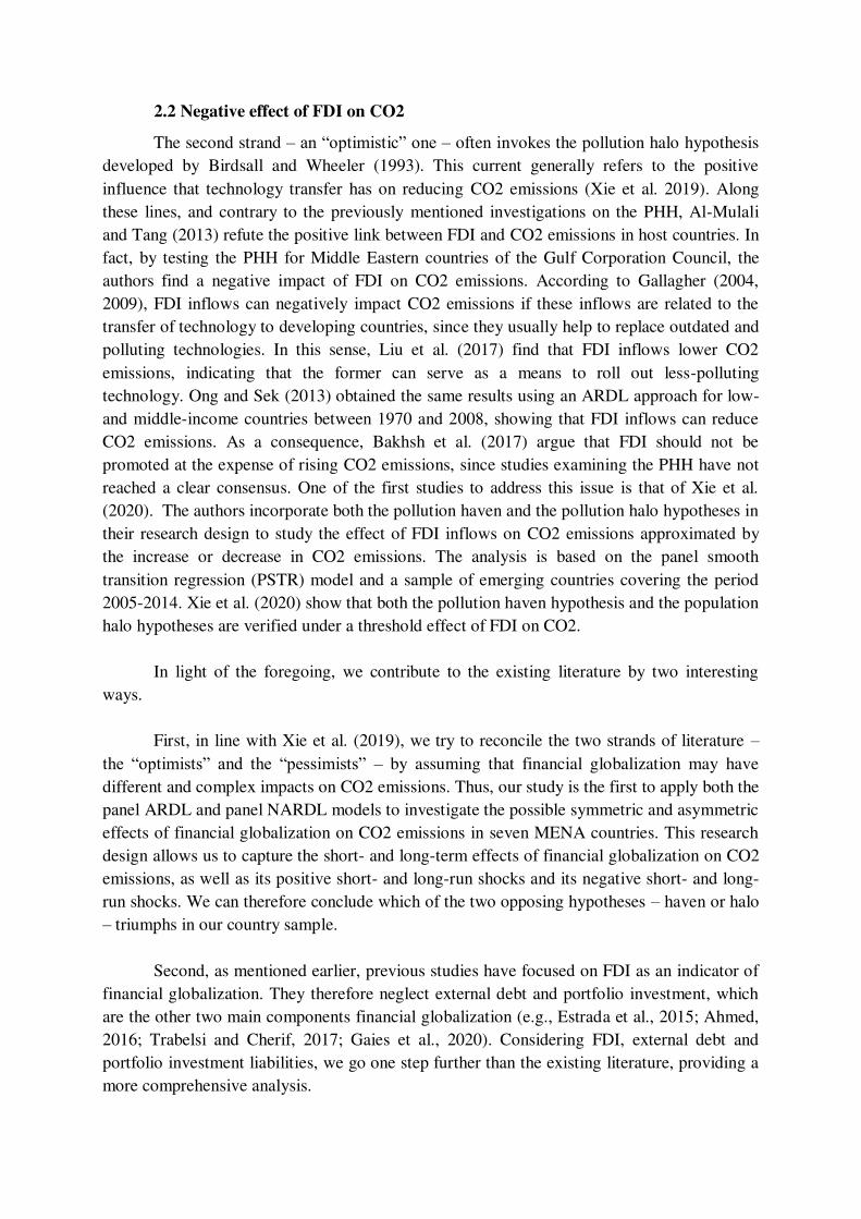
by previous studies. Descriptive statistics for the variables are presented in Table 1 and Figure
1 below.
Table 1. Descriptive statistics
Definition Source Mean Max. Min. Std. Dev. Obs.
CO2 CO2 emissions (Metric tons per capita)
World Bank 6.59 29.98 0.77 8.08 237
DEBT External debt liabilities to GDP
External Wealth of Nations
1.95 16.08 0.09 3.29 237
PORT External portfolio investment liabilities to
GDP
External Wealth of Nations
0.04 0.65 0.00 0.08 237
FDI External FDI liabilities to GDP
External Wealth of Nations
0.33 1.25 0.01 0.27 237
GDP GDP per capita (constant 2010 US $)
World Bank 7501.22 22955.27 1102.35 7284.63 237
EC Energy consumption (kg of oil equivalent per capita)
World Bank 2590.35 12406.75 265.17 3574.11 237
URB Urban population (% of total population) in %
World Bank 67.07 90.00 41.21 16.51 237

0
4
8
12
16
20
24
28
32
Ba
hra
in -
80
Ba
hra
in -
95
Ba
hra
in -
10
Eg
ypt,
Ara
b R
ep
, - 9
0
Eg
ypt,
Ara
b R
ep
, - 0
5
Jo
rda
n -
85
Jo
rda
n -
00
Le
ba
no
n -
80
Le
ba
no
n -
95
Le
ba
no
n -
10
Mo
rocco
- 9
0
Mo
rocco
- 0
5
Om
an
- 8
5
Om
an
- 0
0
Tu
nis
ia -
80
Tu
nis
ia -
95
Tu
nis
ia -
10
CO2
0
4
8
12
16
20
Ba
hra
in -
80
Ba
hra
in -
95
Ba
hra
in -
10
Eg
ypt,
Ara
b R
ep
, - 9
0
Eg
ypt,
Ara
b R
ep
, - 0
5
Jo
rda
n -
85
Jo
rda
n -
00
Le
ba
no
n -
80
Le
ba
no
n -
95
Le
ba
no
n -
10
Mo
rocco
- 9
0
Mo
rocco
- 0
5
Om
an
- 8
5
Om
an
- 0
0
Tu
nis
ia -
80
Tu
nis
ia -
95
Tu
nis
ia -
10
Debt
.0
.1
.2
.3
.4
.5
.6
.7
Ba
hra
in -
80
Ba
hra
in -
95
Ba
hra
in -
10
Eg
ypt,
Ara
b R
ep
, - 9
0
Eg
ypt,
Ara
b R
ep
, - 0
5
Jo
rda
n -
85
Jo
rda
n -
00
Le
ba
no
n -
80
Le
ba
no
n -
95
Le
ba
no
n -
10
Mo
rocco
- 9
0
Mo
rocco
- 0
5
Om
an
- 8
5
Om
an
- 0
0
Tu
nis
ia -
80
Tu
nis
ia -
95
Tu
nis
ia -
10
Portfolio
0.0
0.2
0.4
0.6
0.8
1.0
1.2
1.4
Ba
hra
in -
80
Ba
hra
in -
95
Ba
hra
in -
10
Eg
ypt,
Ara
b R
ep
, - 9
0
Eg
ypt,
Ara
b R
ep
, - 0
5
Jo
rda
n -
85
Jo
rda
n -
00
Le
ba
no
n -
80
Le
ba
no
n -
95
Le
ba
no
n -
10
Mo
rocco
- 9
0
Mo
rocco
- 0
5
Om
an
- 8
5
Om
an
- 0
0
Tu
nis
ia -
80
Tu
nis
ia -
95
Tu
nis
ia -
10
FDI
Figure 1. CO2 and external liabilities evolution over the period 1980-2014
Based on the data presented above, we study the impact of financial globalization on
CO2 emissions using a comprehensive econometric analysis.
First, we test the cross-sectional dependence across our country sample to choose the
adequate panel unit root test (first- or second-generation tests). Second, we check the order of
integration of the variables to verify the use of the ARDL approach. This approach cannot be
adopted if the order of integration exceeds one. Third, we examine the long-run association
among the variables used in our model by applying a set of cointegration tests. Fourth, we
estimate the panel ARDL model explaining the CO2 emissions by the external liabilities and
control variables to investigate the symmetric impact of financial globalization on CO2
emissions in the short- and long-run. Finally, we apply the non-linear panel ARDL approach
(NARDL) to capture the short- and long-term effects of financial globalization on CO2
emissions, as well as its positive short- and long-run shocks and its negative short- and long-
run shocks.

3.2 Cross-sectional dependence and unit root tests
The unit root test is performed for variables to check the order of integration. It is
important to test the cross-sectional dependence for panel datasets in order to choose the
appropriate panel unit root test.4 In homogenous panels, cross-sectional links may emerge
from common economic and/or non-economic macro-dynamics, such as institutional,
demographic, macroeconomic, geographic and/or political aspects. Economic and financial
globalization has increased these common macro-dynamics. Thus, looked at in another way, a
possible cross-sectional dependence in our sample corroborates its homogeneity and could
indicate financial integration between the countries given their geographical position and their
policy of financial openness in a context of financial globalization.
We perform the Breusch and Pagan (1980) 𝐿𝑀 test and the Pesaran (2004) scaled 𝐿𝑀
test to examine the existence of cross-sectional dependence among residuals.
The Lagrange multiplier test proposed by Breusch and Pagan (1980) (𝐿𝑀) is the
appropriate choice when the number of cross section N is smaller than the number of periods
T, which is the case for our framework. To calculate the 𝐿𝑀 statistic, we consider the
following equation: 𝑦𝑖,𝑡 = 𝛼𝑖 + 𝛽′𝑥𝑖,𝑡 + 𝑢𝑖,𝑡 𝑖 = 1, … , 𝑁 and 𝑡 = 1,… , 𝑇 (1) Where 𝑦𝑖,𝑡 is the dependant variable, 𝑥𝑖,𝑡 is a 𝑘 × 1 vector of the explanatory variables, 𝛼𝑖 are the individual intercepts, and 𝛽 is a 𝑘 × 1 vector of the coefficients to be estimated.
Under the null hypothesis of cross-sectional independence, 𝑢𝑖,𝑡 is supposed to be independent
and identically distributed (i.i.d), 𝐻0: 𝜌𝑖𝑗 = 𝜌𝑗𝑖 = 𝑐𝑜𝑟𝑟(𝑢𝑖,𝑡 , 𝑢𝑗,𝑡) = 0 for all t and 𝑖 ≠ 𝑗. Under the alternative hypothesis of cross-sectional dependence, 𝑢𝑖,𝑡 are correlated across
cross-sections, 𝐻1: 𝜌𝑖𝑗 = 𝜌𝑗𝑖 ≠ 0 for at least one pair of 𝑖 ≠ 𝑗. Where 𝜌𝑖𝑗 denotes the pair-
wise correlation of the residuals and expressed as 𝜌𝑖𝑗 = 𝜌𝑗𝑖 = ∑ 𝑢𝑖,𝑡 𝑢𝑗,𝑡𝑇𝑡=1(∑ 𝑢𝑖,𝑡2𝑇𝑡=1 )1 2⁄ (∑ 𝑢𝑗,𝑡2𝑇𝑡=1 )1 2⁄ (2)
The 𝐿𝑀 statistic of Breusch and Pagan is given by: 𝐿𝑀 = 𝑇∑ ∑ �̂�𝑖𝑗2𝑁𝑗=𝑖+1
𝑁−1𝑖=1 (3)
However, the 𝐿𝑀 is not suitable with large N. To resolve this problem, Pesaran (2004)
develops the following scaled version of 𝐿𝑀 test: 𝐶𝐷𝐿𝑀 = √ 1𝑁(𝑁 − 1)∑ ∑ (𝑇�̂�𝑖𝑗2 − 1)𝑁𝑗=𝑖+1
𝑁−1𝑖=1 (4)
4 The panel unit root test is a crucial step because the ARDL approach cannot be performed if the order of integration of our variables exceeds one [I (1)].
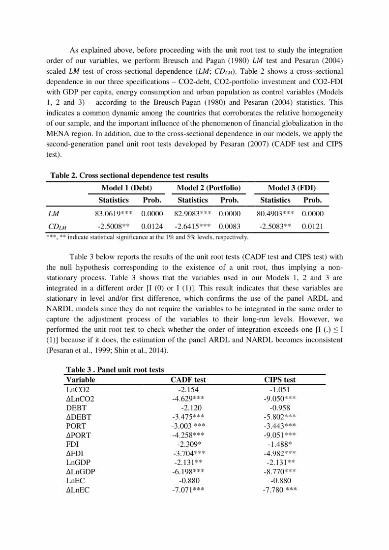
As explained above, before proceeding with the unit root test to study the integration
order of our variables, we perform Breusch and Pagan (1980) 𝐿𝑀 test and Pesaran (2004)
scaled 𝐿𝑀 test of cross-sectional dependence (LM; CDLM). Table 2 shows a cross-sectional
dependence in our three specifications – CO2-debt, CO2-portfolio investment and CO2-FDI
with GDP per capita, energy consumption and urban population as control variables (Models
1, 2 and 3) – according to the Breusch-Pagan (1980) and Pesaran (2004) statistics. This
indicates a common dynamic among the countries that corroborates the relative homogeneity
of our sample, and the important influence of the phenomenon of financial globalization in the
MENA region. In addition, due to the cross-sectional dependence in our models, we apply the
second-generation panel unit root tests developed by Pesaran (2007) (CADF test and CIPS
test).
Table 2. Cross sectional dependence test results
Model 1 (Debt)
Model 2 (Portfolio)
Model 3 (FDI)
Statistics Prob. Statistics Prob. Statistics Prob.
LM 83.0619*** 0.0000
82.9083*** 0.0000
80.4903*** 0.0000
CDLM -2.5008** 0.0124 -2.6415*** 0.0083 -2.5083** 0.0121
***, ** indicate statistical significance at the 1% and 5% levels, respectively.
Table 3 below reports the results of the unit root tests (CADF test and CIPS test) with
the null hypothesis corresponding to the existence of a unit root, thus implying a non-
stationary process. Table 3 shows that the variables used in our Models 1, 2 and 3 are
integrated in a different order [I (0) or I (1)]. This result indicates that these variables are
stationary in level and/or first difference, which confirms the use of the panel ARDL and
NARDL models since they do not require the variables to be integrated in the same order to
capture the adjustment process of the variables to their long-run levels. However, we
performed the unit root test to check whether the order of integration exceeds one [I (.) ≤ I (1)] because if it does, the estimation of the panel ARDL and NARDL becomes inconsistent
(Pesaran et al., 1999; Shin et al., 2014).
Table 3 . Panel unit root tests
Variable CADF test CIPS test
LnCO2 -2.154 -1.051 ∆LnCO2 -4.629*** -9.050*** DEBT -2.120 -0.958 ∆DEBT -3.475*** -5.802*** PORT -3.003 *** -3.443*** ∆PORT -4.258*** -9.051*** FDI -2.309* -1.488* ∆FDI -3.704*** -4.982*** LnGDP -2.131** -2.131** ∆LnGDP -6.198*** -8.770*** LnEC -0.880 -0.880 ∆LnEC -7.071*** -7.780 ***

URB -2.954*** -3.304*** ∆URB -1.948 -0.199 ***, **, * indicate statistical significance at the 1%, 5% and 10% levels, respectively. ∆ is the first difference operator. CADF and CIPS correspond to panel unit root tests proposed by Pesaran (2007). Ln indicates the natural logarithm.
3.3 Cointegration tests
In order to examine the possibility of a long-term relationship between our variables,
we apply the two panel cointegration tests introduced by Pedroni (1999, 2004) and Kao
(1999), with the null hypothesis being the absence of cointegration. Pedroni (1999, 2004)
developed seven tests to test the null hypothesis. Four tests are based on the within-dimension
methods and are computed by separately adding the numerator to the denominator over the N
cross-sections. The other three tests are based on the between-dimension methods and are
computed by splitting the numerator and the denominator prior to summing the N cross-
sections. The Kao (1999) panel cointegration test is based on the ADF test, following the
standard approach adopted by the Engle-Granger step procedures.
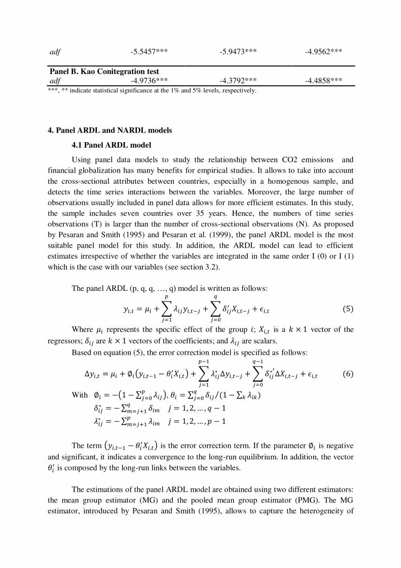
We perform the Pedroni (1999, 2004) and Kao (1999) tests to investigate a potential
long-run relationship between the variables used in our Models 1, 2 and 3, namely CO2
emissions, external debt, FDI and portfolio investment liabilities, GDP per capita, energy
consumption and urban population. The coefficients of these tests are reported in Table 4.
They are mostly significant at the 1% and 5% levels, indicating that co-integration exists
among the variables used in our three Models (1, 2 and 3). In other words, the null hypothesis
of the Pedroni (1999; 2004) and Kao (1999) tests corresponding to non-co-integration is
rejected at the 1% and 5% levels of significance, showing a significant long-term association
between CO2 emissions, external debt, FDI and portfolio investment liabilities, GDP per
capita, energy consumption, and urban population in the sample.
Table 4. Panel cointegration test
Model 1 (Debt)
Model 2 (Portfolio)
Model 3 (FDI)
Statistic
Statistic
Statistic
Panel A. Pedroni Cointegration test common AR coefs. (within-dimension)
v 0.1079
0.3855
-0.2733 rho -1.2273
-1.6538
-0.4445
t -2.8560***
-3.6563***
-1.9819*** adf -2.7265***
-3.6912***
-2.0585***
v (weighted) -1.4808
-0.6962
-1.3623 rho (weighted) -0.4994
-0.2594
-0.6795
t (weighted) -4.3907***
-3.3685***
-3.9477** adf (weighted) -6.0512***
-5.4587***
-4.4299**
individual AR coefs. (between-dimension)
rho -1.0302
-0.9476
-0.8672 t -5.7118***
-5.4731***
-4.9970***
adf -5.5457***
-5.9473***
-4.9562***
Panel B. Kao Conitegration test
adf -4.9736*** -4.3792*** -4.4858*** ***, ** indicate statistical significance at the 1% and 5% levels, respectively.
4. Panel ARDL and NARDL models
4.1 Panel ARDL model
Using panel data models to study the relationship between CO2 emissions and
financial globalization has many benefits for empirical studies. It allows to take into account
the cross-sectional attributes between countries, especially in a homogenous sample, and
detects the time series interactions between the variables. Moreover, the large number of
observations usually included in panel data allows for more efficient estimates. In this study,
the sample includes seven countries over 35 years. Hence, the numbers of time series
observations (T) is larger than the number of cross-sectional observations (N). As proposed
by Pesaran and Smith (1995) and Pesaran et al. (1999), the panel ARDL model is the most
suitable panel model for this study. In addition, the ARDL model can lead to efficient
estimates irrespective of whether the variables are integrated in the same order I (0) or I (1)
which is the case with our variables (see section 3.2).
The panel ARDL (p, q, q, …, q) model is written as follows: 𝑦𝑖,𝑡 = 𝜇𝑖 +∑𝜆𝑖𝑗𝑦𝑖,𝑡−𝑗 +∑𝛿𝑖𝑗′ 𝑋𝑖,𝑡−𝑗 + 𝜖𝑖,𝑡𝑞𝑗=0
𝑝𝑗=1 (5)
Where 𝜇𝑖 represents the specific effect of the group 𝑖; 𝑋𝑖,𝑡 is a 𝑘 × 1 vector of the
regressors; 𝛿𝑖𝑗 are 𝑘 × 1 vectors of the coefficients; and 𝜆𝑖𝑗 are scalars.
Based on equation (5), the error correction model is specified as follows: ∆𝑦𝑖,𝑡 = 𝜇𝑖 + ∅𝑖(𝑦𝑖,𝑡−1 − 𝜃𝑖′𝑋𝑖,𝑡) +∑𝜆𝑖𝑗∗ ∆𝑦𝑖,𝑡−𝑗 +∑𝛿𝑖𝑗∗′∆𝑋𝑖,𝑡−𝑗 + 𝜖𝑖,𝑡𝑞−1𝑗=0
𝑝−1𝑗=1 (6)
With ∅𝑖 = −(1 − ∑ 𝜆𝑖𝑗𝑝𝑗=0 ), 𝜃𝑖 = ∑ 𝛿𝑖𝑗𝑞𝑗=0 (1 − ∑ 𝜆𝑖𝑘𝑘⁄ ) 𝛿𝑖𝑗∗ = −∑ 𝛿𝑖𝑚𝑞𝑚=𝑗+1 𝑗 = 1, 2,… , 𝑞 − 1
𝜆𝑖𝑗∗ = −∑ 𝜆𝑖𝑚𝑝𝑚=𝑗+1 𝑗 = 1, 2,… , 𝑝 − 1
The term (𝑦𝑖,𝑡−1 − 𝜃𝑖′𝑋𝑖,𝑡) is the error correction term. If the parameter ∅𝑖 is negative
and significant, it indicates a convergence to the long-run equilibrium. In addition, the vector 𝜃𝑖′ is composed by the long-run links between the variables.
The estimations of the panel ARDL model are obtained using two different estimators:
the mean group estimator (MG) and the pooled mean group estimator (PMG). The MG
estimator, introduced by Pesaran and Smith (1995), allows to capture the heterogeneity of

long-run and short-run parameters. It estimates equations for each individual country and then
calculates the coefficients’ means. Thus, the possible homogeneity across countries is not
taken into account. The PMG estimator, developed by Pesaran et al. (1999), allows the short-
run coefficients to vary across countries, however, it assumes that the long-run coefficients
are the same among countries (Dimitriadis and Katrakilidis, 2020). After running the MG and
PMG models, it is necessary to choose the best estimator. For this purpose, the Hausman test
is performed to compare the long-run coefficients of these estimators. If the null hypothesis is
not rejected, the PMG estimator is preferred. If the alternative hypothesis is accepted, the MG
estimator is more appropriate.
In order to study the impact of financial globalization on CO2 emissions , we develop
the following model: 𝐿𝑛𝐶𝑂2𝑖,𝑡 = 𝛽0𝑖 + 𝛽1𝑖𝐺𝐿𝑂𝐵𝑖,𝑡 + 𝛽2𝑖𝐿𝑛𝐺𝐷𝑃𝑖,𝑡 + 𝛽3𝑖𝐿𝑛𝐸𝐶𝑖,𝑡 + 𝛽4𝑖𝑈𝑅𝐵𝑖,𝑡 + 𝑢𝑖,𝑡 (7)
Where 𝐿𝑛𝐶𝑂2𝑖,𝑡, 𝐺𝐿𝑂𝐵𝑖,𝑡, 𝐿𝑛𝐺𝐷𝑃𝑖,𝑡, 𝐿𝑛𝐸𝐶𝑖,𝑡 and 𝑈𝑅𝐵𝑖,𝑡 represent respectively the
natural logarithm of CO2 emissions per capita, the financial globalization indicators (debt,
portfolio investment and FDI liabilities), the natural logarithm of GDP per capita, the natural
logarithm of the per capita energy consumption, and the urban population. 𝑢𝑖,𝑡 is the error
term.
According to Peseran et al. (1999), the ARDL model is written as follows: 𝐿𝑛𝐶𝑂2𝑖,𝑡 = µ𝑖 +∑𝜆𝑖𝑗𝐿𝑛𝐶𝑂2𝑖,𝑡−𝑗 +∑𝛿1𝑖𝑗𝐺𝐿𝑂𝐵𝑖,𝑡−𝑗 +𝑞𝑗=0
𝑝𝑗=1 ∑𝛿2𝑖𝑗𝐿𝑛𝐺𝐷𝑃𝑖,𝑡−𝑗𝑞
𝑗=0+∑𝛿3𝑖𝑗𝐿𝑛𝐸𝐶𝑖,𝑡−𝑗 +∑𝛿4𝑖𝑗𝑈𝑅𝐵𝑖,𝑡−𝑗 +𝑞𝑗=0 𝜀𝑖,𝑡 (8)𝑞
𝑗=0
The Schwarz Bayesian Criterion (SBC) criterion and the Akaike Information Criterion
(AIC) are employed to select the appropriate lag length.
Based on Peseran et al. (1999, 2001), equation (8) can be presented as follows:
∆𝐿𝑛𝐶𝑂2𝑖,𝑡 = 𝜇𝑖 + 𝛾1𝑖𝐿𝑛𝐶𝑂2𝑖,𝑡−1 + 𝛾2𝑖𝐺𝐿𝑂𝐵𝑖,𝑡−1 + 𝛾3𝑖𝑙𝑛𝐺𝐷𝑃𝑖,𝑡−1 + 𝛾4𝑖𝐿𝑛𝐺𝐷𝑃𝑖,𝑡−1+ 𝛾5𝑖𝑈𝑅𝐵𝑖,𝑡−1 +∑𝜆𝑖𝑗∆𝐿𝑛𝐶𝑂2𝑖,𝑡−𝑗 +∑𝛿1𝑖𝑗∆𝐺𝐿𝑂𝐵𝑖,𝑡−𝑗𝑞−1𝑗=0
𝑝−1𝑗=1+∑𝛿2𝑖𝑗∆𝑙𝑛𝐺𝐷𝑃𝑖,𝑡−𝑗 +𝑞−1
𝑗=0 ∑𝛿3𝑖𝑗∆𝐿𝑛𝐸𝐶𝑖,𝑡−𝑗 +∑𝛿4𝑖𝑗∆𝑈𝑅𝐵𝑖,𝑡−𝑗𝑞−1𝑗=0
𝑞−1𝑗=0+ 𝜀𝑖,𝑡 (9)
Where ∆ is the first difference operator; 𝜇 is the constant; 𝜆𝑖𝑗 and 𝛿𝑠𝑖𝑗(𝑠=1,2,3,4) are the
short-run coefficients of the dependant and independent variables, respectively; and 𝜀𝑖,𝑡 is the
error term.

In order to incorporate an error correction term, equation (9) can be rewritten as
follows: ∆𝐿𝑛𝐶𝑂2𝑖,𝑡 = 𝜇𝑖 +∑𝜆𝑖𝑗∆𝐿𝑛𝐶𝑂2𝑖,𝑡−𝑗 +∑𝛿1𝑖𝑗∆𝐺𝐿𝑂𝐵𝑖,𝑡−𝑗𝑞−1𝑗=0
𝑝−1𝑗=1+∑𝛿2𝑖𝑗∆𝑙𝑛𝐺𝐷𝑃𝑖,𝑡−𝑗 +𝑞−1
𝑗=0 ∑𝛿3𝑖𝑗∆𝐿𝑛𝐸𝐶𝑖,𝑡−𝑗 +∑𝛿4𝑖𝑗∆𝑈𝑅𝐵𝑖,𝑡−𝑗 +𝑞−1𝑗=0
𝑞−1𝑗=0+ ∅𝑖𝐸𝐶𝑇𝑖,𝑡−1 + 𝜀𝑖,𝑡 (10)
Where 𝐸𝐶𝑇𝑖,𝑡−1 = (𝐿𝑛𝐶𝑂2𝑖,𝑡−1 − 𝜃1𝑖𝐺𝐿𝑂𝐵𝑖,𝑡−1 − 𝜃2𝑖𝐿𝑛𝐺𝐷𝑃𝑖,𝑡−1 − 𝜃3𝑖𝐿𝑛𝐸𝐶𝑖,𝑡−1 −𝜃4𝑖𝑈𝑅𝐵𝑖,𝑡−1) is the error correction term; and ∅𝑖 is the speed of adjustment of the model to
the long-run equilibrium. 𝜃1𝑖 , 𝜃2𝑖 , 𝜃3𝑖 𝑎𝑛𝑑 𝜃4𝑖 represent the long-run coefficients, and they are
calculated as 𝛾2𝑖 𝛾1𝑖⁄ , 𝛾3𝑖 𝛾1𝑖⁄ , 𝛾4𝑖 𝛾1𝑖⁄ and 𝛾5𝑖 𝛾1𝑖⁄ , respectively.
As mentioned above, we apply the panel ARDL estimation to capture the symmetric
impact of external liabilities (financial globalization indicators) on CO2 emissions (CO2
emissions indicator) for our sample of seven MENA countries for the years 1980 to 2014. As
shown in Table 5, the Hausman statistics indicate that the maximum likelihood-based PMG
estimator is more efficient than the maximum likelihood-based MG estimator at the
significance level of 5%, which led us to apply the PMG model, as suggested by Pesaran et al.
(1999). In addition, Table 5 reports the long- and short-run coefficients of the external
liabilities indicators and the other explanatory variables. It displays a positive and significant
long-run coefficient of debt liabilities at the 10% level, while the long-run coefficients of FDI
and portfolio investment liabilities are statistically non-significant at conventional levels. The
table also shows that the long-run coefficients of GDP per capita and energy consumption are
positively and significantly linked to CO2 emissions. However, the model does not capture a
significant long-run impact of urban population on CO2 emissions. With regard to the short-
run coefficients, Table 5 reveals that only the effect of urban population on CO2 emissions is
positive and significant at the 5% level. Finally, the negative and significant coefficients of
error correction term (ECT (-1)) at the 1% level, prove that a significant link exists between
the short-and long-run effects captured by our model.
Table 5. Linear Panel ARDL results
Model 1 (Debt)
Model 2 (Portfolio)
Model 3 (FDI)
Variable Coef. Std. Err Coef. Std. Err Coef. Std. Err
Long-Run Coefficients
DEBT 0.0167* 0.0095
-0.0910 0.0910
-0.0171 0.0342
(0.077)
(0.317)
(0.618) LnGDP 0.2146*** 0.0658
0.1372** 0.0631
0.1743*** 0.0651
(0.001)
(0.030)
(0.007) LnEC 0.7265*** 0.0765
0.7876*** 0.0778
0.7737*** 0.0721

(0.000)
(0.000)
(0.000) URB -0.0022 0.0013
0.0003 0.0014
-0.0012 0.0013
(0.104)
(0.811)
(0.338)
Error correction Coefficient
ECT(-1) -0.5619*** 0.1655
-0.5635*** 0.1649
-0.5783*** 0.1702
(0.001)
(0.001)
(0.001)
Short-Run Coefficients
DEBT -0.0141 0.0416
-0.2691 0.4715
-0.0932 0.1237
(0.734)
(0.568)
(0.451) LnGDP -0.0670 0.0480
-0.0041 0.0728
-0.0258 0.0687
(0.163)
(0.955)
(0.707) LnEC 0.1617 0.1779
0.1463 0.1656
0.1365 0.1831
(0.363)
(0.377
(0.456) URB 0.2038** 0.1029
0.2191** 0.0993
0.2199** 0.1083
(0.048)
(0.027)
(0.042) Intercept -3.1671*** 0.9540
-3.1348*** 0.9420
-3.2718*** 0.9857
(0.001)
(0.001)
(0.001)
Hausman test 8.93 (0.0629)
8.67 (0.0701)
6.46 (0.1676)
N° Obs. 230
230
230
Log Likelihood 392.3161 391.8918 394.0558 Note: ***, **, * indicate statistical significance at the 1%, 5% and 10% levels, respectively. Values in parenthesis are probabilities. Ln indicates the natural logarithm.
4.2. Non-linear panel ARDL (NARDL) model
In order to take into account the long- and short-run asymmetries in the impact of
financial globalization on CO2 emissions , we perform the non-linear ARDL (NARDL)
model proposed by Shin et al. (2014). Using this approach, the value of the financial
globalization (GLOB) indicators (Debt, Portfolio and FDI) are divided into positive and
negative shocks, noted respectively as 𝐺𝐿𝑂𝐵𝑖,𝑡+ and 𝐺𝐿𝑂𝐵𝑖,𝑡− . The positive and negative partial
sums decompositions of financial globalization are computed as:
{ 𝐺𝐿𝑂𝐵𝑖,𝑡+ =∑∆𝐺𝐿𝑂𝐵𝑖,𝑗+𝑡
𝑗=1 =∑𝑚𝑎𝑥 (∆𝐺𝐿𝑂𝐵𝑖,𝑗+ , 0)𝑡𝑗=1𝐺𝐿𝑂𝐵𝑖,𝑡− =∑∆𝐺𝐿𝑂𝐵𝑖,𝑗−𝑡
𝑗=1 =∑𝑚𝑖𝑛 (∆𝐺𝐿𝑂𝐵𝑖,𝑗− , 0)𝑡𝑗=1
(11)
By replacing 𝐺𝐿𝑂𝐵𝑖+ and 𝐺𝐿𝑂𝐵𝑖− into 𝐺𝐿𝑂𝐵𝑖 in equation (9), we obtain the following
non-linear panel ARDL model:

∆𝐿𝑛𝐶𝑂2𝑖,𝑡 = 𝜇𝑖 + 𝛾1𝑖𝐿𝑛𝐶𝑂2𝑖,𝑡−1 + 𝛾2𝑖+𝐺𝐿𝑂𝐵𝑖,𝑡−1+ + 𝛾2𝑖−𝐺𝐿𝑂𝐵𝑖,𝑡−1− + 𝛾3𝑖𝑙𝑛𝐺𝐷𝑃𝑖,𝑡−1+ 𝛾4𝑖𝐿𝑛𝐺𝐷𝑃𝑖,𝑡−1 + 𝛾5𝑖𝑈𝑅𝐵𝑖,𝑡−1+∑𝜆𝑖𝑗∆𝐿𝑛𝐶𝑂2𝑖,𝑡−𝑗 +∑(𝛿1𝑖𝑗+ ∆𝐺𝐿𝑂𝐵𝑖,𝑡−𝑗+ + 𝛿1𝑖𝑗− ∆𝐺𝐿𝑂𝐵𝑖,𝑡−𝑗− )𝑞−1𝑗=0
𝑝−1𝑗=1+∑𝛿2𝑖𝑗∆𝑙𝑛𝐺𝐷𝑃𝑖,𝑡−𝑗 +𝑞−1𝑗=0 ∑𝛿3𝑖𝑗∆𝐿𝑛𝐸𝐶𝑖,𝑡−𝑗 +∑𝛿4𝑖𝑗∆𝑈𝑅𝐵𝑖,𝑡−𝑗𝑞−1
𝑗=0𝑞−1𝑗=0+ 𝜀𝑖,𝑡 (12)
Where 𝛿1𝑖𝑗+ and 𝛿1𝑖𝑗− are the short-run coefficients associated with positive and negative
shocks, respectively.
The error correction version of the equation (12) is expressed as follows: ∆𝐿𝑛𝐶𝑂2𝑖,𝑡 = 𝜇𝑖 +∑𝜆𝑖𝑗∆𝐿𝑛𝐶𝑂2𝑖,𝑡−𝑗 +∑(𝛿1𝑖𝑗+ ∆𝐺𝐿𝑂𝐵𝑖,𝑡−𝑗+ + 𝛿2𝑖−∆𝐺𝐿𝑂𝐵𝑖,𝑡−𝑗− )𝑞−1𝑗=0
𝑝−1𝑗=1+∑𝛿2𝑖𝑗∆𝑙𝑛𝐺𝐷𝑃𝑖,𝑡−𝑗 +𝑞−1
𝑗=0 ∑𝛿3𝑖𝑗∆𝐿𝑛𝐸𝐶𝑖,𝑡−𝑗 +∑𝛿4𝑖𝑗∆𝑈𝑅𝐵𝑖,𝑡−𝑗𝑞−1𝑗=0
𝑞−1𝑗=0+ ∅𝑖𝐸𝐶𝑇𝑖,𝑡−1 + 𝜀𝑖,𝑡 (13)
Where 𝐸𝐶𝑇𝑖,𝑡−1 = (𝐿𝑛𝐶𝑂2𝑖,𝑡−1 − 𝜃1𝑖+𝐺𝐿𝑂𝐵𝑖,𝑡−1+ − 𝜃1𝑖−𝐺𝐿𝑂𝐵𝑖,𝑡−1− − 𝜃2𝑖𝐿𝑛𝐺𝐷𝑃𝑖,𝑡−1 −𝜃3𝑖𝐿𝑛𝐸𝐶𝑖,𝑡−1 − 𝜃4𝑖𝑈𝑅𝐵𝑖,𝑡−1) is the error correction term. 𝜃1𝑖+ and 𝜃1𝑖− represent the long-run
coefficients associated with positive and negative shocks, respectively. These coefficients are
calculated as: 𝜃1𝑖+ = 𝛾2𝑖+ 𝛾1𝑖⁄ and 𝜃1𝑖− = 𝛾2𝑖− 𝛾1𝑖⁄ .
The mitigated effects of FDI inflows on CO2 (the pollution haven hypothesis vs the
pollution halo hypothesis) that emerged from previous studies (see Section 2), as well as the
non-significant symmetric impacts of FDI and portfolio investment liabilities on CO2,
highlighted by our panel ARDL estimates, led us to reconduct our regressions by applying the
panel NARDL model developed by Shin et al. (2014). The panel NARDL results are presented
in Table 6 which includes the long- and short-run coefficients of the external liabilities variables,
as well as GDP per capita, energy consumption and urban population. In addition, Table 6
reports the results of the Wald symmetry test which highlights the existence of long-term
asymmetric effects at the 5% level for the FDI-CO2 nexus (Model 2) and the portfolio
investment-CO2 nexus (Model 3), while the test indicates an absence of asymmetric effects
for the external debt-CO2 nexus (Model 1) and for all models in the short term. The long-run
coefficients of Models 2 and 3 reveal that a negative shock of FDI and portfolio investment
liabilities decreases CO2 emissions. Thus, it appears that financial globalization through
foreign investment is more environmentally friendly than financial globalization through debt
(Table 5) for MENA countries. Moreover, the estimates of Models 2 and 3 show a posit ive
impact of energy consumption, GDP per capita and urban population on CO2 emissions in the
long run. The Hausman test statistics in Table 6 approve the use of the PMG model as is the

case with the panel ARDL model (Table 5), and the negative and significant coefficients of
the error correction term (ECT (-1)) at the 1% level confirm the convergence between the
short- and the long-run shocks.
Table 6. Non Linear Panel ARDL results
Model 1 (Debt)
Model 2 (Portfolio)
Model 3 (FDI)
Variable Coef. Std. Err Coef. Std. Err Coef. Std. Err
Long-Run Coefficients
GLOB+ 0.0244 0.0203
0.0366 0.0771
0.0062 0.0328
(0.231)
(0.635)
(0.851) GLOB- 0.0201 0.0126
0.2268** 0.1055
0.1890*** 0.0556
(0.111)
(0.032)
(0.001) LnGDP 0.2044*** 0.0656
0.1376*** 0.0531
0.1805*** 0.0624
(0.002)
(0.009)
(0.004) LnEC 0.7749*** 0.0737
0.7603*** 0.0742
0.8267*** 0.0646
(0.000)
(0.000)
(0.000) URB -0.0030** 0.0015
0.0044*** 0.0017
0.0030* 0.0015
(0.038)
(0.008)
(0.054)
Error correction Coefficient
ECT(-1) -0.6039*** 0.1520
-0.6674*** 0.1676
-0.6679*** 0.1667
(0.000)
(0.000
(0.000)
Short-Run Coefficients
GLOB+ 0.0118 0.1317
0.3419 0.7172
-0.0502 0.0914
(0.929)
(0.634)
(0.583) GLOB- -0.0701 0.1293
-1.1060 0.8580
-0.6498 0.3983
(0.588)
(0.197)
(0.103) LnGDP -0.0387 0.0545
-0.0669 0.0787
-0.0464 0.0658
(0.478)
(0.395)
(0.481) LnEC 0.1145 0.1857
0.0575 0.1360
0.0185 0.1705
(0.537)
(0.672)
(0.914) URB 0.2220** 0.1084
0.2283** 0.0926
0.2371** 0.1183
(0.040)
(0.014)
(0.045) Intercept -3.5172*** 0.9028
-3.7670*** 0.9693
-4.2239*** 1.0571
(0.000) (0.000) (0.000)
Long run asymmetry test
WLR 0.18 (0.6714)
12.15*** (0.0005)
14.81*** (0.0001)
Short run asymmetry test
WSR 0.11 (0.7391) 1.81 (0.1781) 2.69 (0.1011)
Hausman test 2.79 (0.7321)
7.2700 (0.2012)
0.85 (0.9741)
N° Obs. 224
224
224
Log Likelihood 386.5126 386.8562 394.1522 Note: ***, **, * indicate statistical significance at the 1%, 5% and 10% levels, respectively. Values in parenthesis are probabilities. Ln indicates the natural logarithm.

In summary, our results confirm that the relationship between financial globalization
and CO2 emissions is complex and multifaceted. They reveal that in the seven MENA
countries we studied over the period 1980-2014, CO2 emissions are significantly impacted in
the long term by external liabilities, while in the short term, this impact does not seem to be
really significant. The long-run impact of financial globalization on CO2 emissions can be
symmetric and asymmetric depending on the nature of this globalization. When financial
globalization is based on debt liabilities, it seems risky for the climate because it increases
CO2 emissions significantly and linearly. In contrast, the long-term impact of FDI and
portfolio investment liabilities on CO2 emissions is asymmetric, with only negative shocks of
FDI and portfolio investment decreasing CO2 emissions, thus demonstrating that a lower
stock of FDI and portfolio investment equals higher CO2 emissions. It appears that financial
globalization based on foreign investment (FDI and portfolio investment) is more
environmentally friendly than financial globalization based on external debt. This can be
explained by the fact that foreign investment, in particular FDI, unlike external debt, has a
positive spillover effect on the climate by bringing green and ethical businesses and
technologies that reduce CO2 emissions in recipient countries. It goes without saying that, in
the meantime, FDI and portfolio investment can catalyze CO2 emissions in recipient
countries, particularly developing countries, which aim to promote economic growth by
relaxing environmental regulations to attract foreign capital. However, it appears from our
panel NARDL results that only the environmentally beneficial effect of foreign investment
(FDI and portfolio investment) is significant in the long term. This refutes the pollution haven
hypothesis in favor of the pollution halo hypothesis. On the contrary, external debt does not
ensure technology transfer. They could allow the financing of economic growth through the
mobilization of foreign capital, but without a positive spillover effect on the environment,
worse still, they increase CO2 emissions. This could be explained by the fact that in our seven
MENA countries, external debt is oriented towards consumption and polluting production.
The long-term positive impact of our control variables – GDP per capita, energy consumption
and urban population – on CO2 emissions corroborates this pattern.
5. Conclusion
In this paper, we studied the symmetric and asymmetric effects that financial globalization may have on CO2 emissions in the MENA region. Covering the period 1980-2014 for seven non-OPEC MENA countries, we applied the panel ARDL and NARDL models. As part of this comprehensive econometric investigation, we also conducted a battery of tests, including cross-sectional dependence tests, second-generation unit root tests and cointegration tests. Our results show a significant long-term impact of financial globalization on CO2 emissions. Depending on the nature of financial globalization – achieved through external debt or foreign investment (FDI and portfolio investment) – the impact can be either symmetric or asymmetric. As for external debt, it increases CO2 emissions in a significant and linear way and therefore constitutes CO2 emissions. On the contrary, since the long-term impact of FDI and portfolio investment liabilities on CO2 emissions is asymmetric, only negative shocks of both FDI and portfolio investment liabilities decrease CO2 emissions, while positive shocks do not increase CO2 emissions. In other words, this suggests that financial globalization through foreign investment is more respectful of the environment than financial globalization
through debt. These results can be explained by the fact that foreign investment in general and FDI in particular contributes to the establishment of green businesses and technologies in recipient countries that help reduce CO2 emissions, as opposed to external debt. In fact, not only does the latter fail to ensure the transfer of technology, but it also increases CO2 emissions, as the mobilization of foreign capital to finance economic growth does not have a positive spillover effect on the environment. This could be explained by the fact that in our seven MENA countries, external debt is oriented towards consumption and polluting production. In summary and drawing on our findings, we can refute the pollution haven hypothesis in favor of the pollution halo hypothesis. These results provide interesting insights for policy makers in MENA countries by highlighting the relevance of strict regulation of foreign capital flows, apart from portfolio investment and FDI, to reduce CO2 emissions and address the climate challenge. In future research, we suggest comparing the results of these non-OPEC MENA countries with other non-oil exporting emerging countries, as they are also subject to almost the same economic, social and environmental constraints.
Author Declarations
-Funding: Not applicable'
-Conflicts of interest/Competing interests (include appropriate disclosures): Not applicable'
-Availability of data and material/ Data availability (data transparency, if link please provide
the link to access. For further information, go to -
https://www.springernature.com/gp/authors/research-data-policy/data-availability-
statements/12330880): Not applicable'
-Code availability (software application or custom code): Not applicable'
Authors' contributions
Brahim Gaies: Conceptualization, Literature review, Methodology, Result interpretations,
Discussion and Implications, Original draft.
Mohamed Sahbi Nakhli: Methodology, Empirical study, Writing Results.
Jean Michel Sahut: Conceptualization, Data collection, Introduction, Discussion and
Implications, Conclusion, Abstract, Editing review.

References
Abdouli, M., & Hammami, S. (2017). Economic growth, FDI inflows and their impact on the
environment: an empirical study for the MENA countries. Quality & Quantity, 51(1),
121-146. Ahmed, A. D. (2016). Integration of financial markets, financial development and growth: Is
Africa different?. Journal of International Financial Markets, Institutions and Money,
42, 43-59.
Ahmed, A. D. (2016). Integration of financial markets, financial development and growth: Is
Africa different?. Journal of International Financial Markets, Institutions and Money,
42, 43-59.
Al-Mulali, U., & Tang, C. F. (2013). Investigating the validity of pollution haven hypothesis
in the gulf cooperation council (GCC) countries. Energy Policy, 60, 813-819. Bakhsh, K., Rose, S., Ali, M. F., Ahmad, N., & Shahbaz, M. (2017). Economic growth, CO2
emissions, renewable waste and FDI relation in Pakistan: New evidences from
3SLS. Journal of Environmental Management, 196, 627-632.
Boufateh, T., & Saadaoui, Z. (2020). Do Asymmetric Financial Development Shocks Matter
for CO 2 Emissions in Africa? A Nonlinear Panel ARDL–PMG Approach.
Environmental Modeling & Assessment, 25(6), 809-830. Breusch, TS., & Pagan, AR. (1980) The Lagrange multiplier test and its applications to model
specification in econometrics. The Review of Economic Studies 47: 239-253.
Chen, H., O. Hongo, D., Ssali, M.W., Nyaranga, M.S., & Wairimu Nderitu, C. (2020). The
Asymmetric Influence of Financial Development on Economic Growth in Kenya:
Evidence From NARDL. SAGE Open, 10(1), 21582440198.
Dimitriadis, D., & Katrakilidis, C. (2020). An empirical analysis of the dynamic interactions
among ethanol, crude oil and corn prices in the US market. Annals of Operations
Research, 294(1), 47-57.
Estrada, G. B., Park, D., & Ramayandi, A. (2015). Financial development, financial openness,
and economic growth. Asian Development Bank Economics Working Paper Series,
(442).
Gaies, B., & Nabi, M. S. (2019). Financial Openness and Growth in Developing Countries.
Journal of Economic Integration, 34(3), 426-464.
Gaies, B., Goutte, S., & Guesmi, K. (2020). Does financial globalization still spur growth in
emerging and developing countries? Considering exchange rates. Research in
International Business and Finance, 52, 101-113.
Gallagher, K. (2004). Free trade and the environment: Mexico, NAFTA, and beyond. Stanford
University Press. Gallagher, K. P. (2009). Economic globalization and the environment. Annual Review of
Environment and Resources, 34, 279-304.
Gilmont, M. (2015). Water resource decoupling in the MENA through food trade as a
mechanism for circumventing national water scarcity. Food Security, 7(6), 1113-1131.
Hakimi, A., & Hamdi, H. (2017). Does corruption limit FDI and economic growth? Evidence
from MENA countries. International Journal of Emerging Markets, Vol. 12 No. 3, pp.
550-571.

Kaab, A., Sharifi, M., Mobli, H., Nabavi-Pelesaraei, A., & Chau, K. W. (2019). Combined
life cycle assessment and artificial intelligence for prediction of output energy and
environmental impacts of sugarcane production. Science of the Total
Environment, 664, 1005-1019. Kao C. (1999) Spurious regression and residual-based tests for cointegration in panel data.
Journal of Econometrics 90: 1-44.
Kari, F., & Saddam, A. (2012). Growth, FDI, imports, and their impact on carbon dioxide
emissions in GCC countries: an empirical study. Mediterr. J. Soc. Sci, 3, 25-31. Koçak, E., & Şarkgüneşi, A. (2018). The impact of foreign direct investment on CO 2
emissions in Turkey: new evidence from cointegration and bootstrap causality
analysis. Environmental Science and Pollution Research, 25(1), 790-804. Lan, J., Kakinaka, M., & Huang, X. (2012). Foreign direct investment, human capital and
environmental pollution in China. Environmental and Resource Economics, 51(2),
255-275. Lane, P. R., & Milesi-Ferretti, G. M. (2018). The external wealth of nations revisited:
international financial integration in the aftermath of the global financial crisis. IMF
Economic Review, 66(1), 189-222.
Levy-Yeyati, E., & Williams, T. (2011). Financial globalization in emerging economies:
Much ado about nothing? Business School Working Papers 2011-01, Universidad
Torcuato Di Tella.
Liu, Y., Hao, Y., & Gao, Y. (2017). The environmental consequences of domestic and foreign
investment: Evidence from China. Energy Policy, 108, 271-280.
Nabavi-Pelesaraei, A., Rafiee, S., Mohtasebi, S. S., Hosseinzadeh-Bandbafha, H., & Chau, K.
W. (2018). Integration of artificial intelligence methods and life cycle assessment to
predict energy output and environmental impacts of paddy production. Science of the
total environment, 631, 1279-1294. Nasir, M. A., Huynh, T. L. D., & Tram, H. T. X. (2019). Role of financial development,
economic growth & foreign direct investment in driving climate change: A case of
emerging ASEAN. Journal of environmental management, 242, 131-141. Neequaye, N. A., & Oladi, R. (2015). Environment, growth, and FDI revisited. International
Review of Economics & Finance, 39, 47-56.
Omri, A., Nguyen, D.K., & Rault, C. (2014). Causal interactions between CO2 emissions,
FDI, and economic growth: Evidence from dynamic simultaneous-equation models.
Economic Modelling, 42(C), 382-389.
Ong, S. M., & Sek, S. K. (2013). Interactions between economic growth and environmental
quality: panel and non-panel analyses. Applied Mathematical Sciences, 7(14), 687-
700. Ouyang, X., & Lin, B. (2015). An analysis of the driving forces of energy-related carbon
dioxide emissions in China’s industrial sector. Renewable and sustainable energy
reviews, 45, 838-849. Pedroni P. (1999) Critical values for cointegration tests in heterogeneous panels with multiple
Pedroni P. (2004) Panel cointegration: asymptotic and finite sample properties of pooled time
series tests with an application to the PPP hypothesis. Econometric Theory 20: 597-
625.

Pesaran MH & Smith R. (1995) Estimating long-run relationships from dynamic
heterogeneous panels. Journal of Econometrics 68: 79-113.
Pesaran MH, Shin Y & Smith RJ. (2001) Bounds testing approaches to the analysis of level
Pesaran MH, Shin Y & Smith RP. (1999) Pooled mean group estimation of dynamic
heterogeneous panels. Journal of the American Statistical Association 94: 621-634.
Pesaran, H. M. (2004). General diagnostic tests for cross-sectional dependence in panels.
University of Cambridge, Cambridge Working Papers in Economics, 435.
Pesaran, M.H., (2007). A simple panel unit root test in the presence of cross-section
independence. Journal of Applied Econometrics. 22 (2), 265-312.
Pethig, R. (1976). Pollution, welfare, and environmental policy in the theory of comparative
advantage. Journal of environmental economics and management, 2(3), 160-169. Radermacher, F.J. (1994). Environmental systems and economics: The main issues a panel
discussion. Annals of Operations Research, 54, 1-14.
Raggad, B. (2020). Economic development, energy consumption, financial development, and
carbon dioxide emissions in Saudi Arabia: new evidence from a nonlinear and
asymmetric analysis. Environmental Science and Pollution Research, 27(17), 21872-
21891.
Shahbaz, M., Gozgor, G., Adom, P. K., & Hammoudeh, S. (2019). The technical
decomposition of carbon emissions and the concerns about FDI and trade openness
effects in the United States. International Economics, 159, 56-73. Shahbaz, M., Nasreen, S., Abbas, F., & Anis, O. (2015). Does foreign direct investment
impede environmental quality in high-, middle-, and low-income countries?. Energy
Economics, 51, 275-287. Shin Y, Yu B & Greenwood-Nimmo M. (2014) Modelling asymmetric cointegration and
dynamic multipliers in a nonlinear ARDL framework. Festschrift in Honor of Peter
Schmidt. Springer, 281-314.
Sinha, A., Shahbaz, M., & Balsalobre, D. (2017). Exploring the relationship between energy
usage segregation and environmental degradation in N-11 countries. Journal of
Cleaner Production, 168, 1217-1229. Solarin, S. A., Al-Mulali, U., Musah, I., & Ozturk, I. (2017). Investigating the pollution haven
hypothesis in Ghana: an empirical investigation. Energy, 124, 706-719. Trabelsi, M., & Cherif, M. (2017). Capital account liberalization and financial deepening:
Does the private sector matter?. The Quarterly Review of Economics and Finance, 64,
141-151.
Walter, I., & Ugelow, J. L. (1979). Environmental policies in developing countries. Ambio,
102-109.
Xiao-Lin, L., Xin, L., & Deng-Kui, S. (2020). Asymmetric determinants of corporate bond
credit spreads in China: Evidence from a nonlinear ARDL model, The North
American Journal of Economics and Finance, 52(C), 101109.
Xie, Q., Wang, X., & Cong, X. (2020). How does foreign direct investment affect CO2
emissions in emerging countries? New findings from a nonlinear panel
analysis. Journal of Cleaner Production, 249, 119422.

Figures
Figure 1
CO2 and external liabilities evolution over the period 1980-2014