IS* curve to the left. If curve is unaffected. As shown in ...qed.econ.queensu.ca/pub/students/khans/ECON2450_AS4_SOL.pdf · the exchange rate floats freely, then the LM* curve is

QQuueessttiioonnss ffoorr RReevviieeww1. In the Mundell–Fleming model, an increase in taxes shifts the IS* curve to the left. If

the exchange rate floats freely, then the LM* curve is unaffected. As shown in Figure12–1, the exchange rate falls while aggregate income remains unchanged. The fall inthe exchange rate causes the trade balance to increase.

111

A

B

YIncome, output

e

Exc

hang

e ra

te

IS2*

*IS1

LM*

FFiigguurree 1122––11

C H A P T E R 12 Aggregate Demand in the

Open Economy

Now suppose there are fixed exchange rates. When the IS* curve shifts to the leftin Figure 12–2, the money supply has to fall to keep the exchange rate constant, shift-ing the LM* curve from LM to LM . As shown in the figure, output falls while theexchange rate remains fixed.

Net exports can only change if the exchange rate changes or the net exports sched-ule shifts. Neither occurs here, so net exports do not change.

We conclude that in an open economy, fiscal policy is effective at influencing out-put under fixed exchange rates but ineffective under floating exchange rates.

2. In the Mundell–Fleming model with floating exchange rates, a reduction in the moneysupply reduces real balances M/P, causing the LM* curve to shift to the left. As shownin Figure 12–3, this leads to a new equilibrium with lower income and a higherexchange rate. The increase in the exchange rate reduces the trade balance.

112 Answers to Textbook Questions and Problems

*1

*2

AB

Y

e

e

Exc

hang

e ra

te

Fixedexchange rate

IS2

IS1

Income, output

Y1

LM2

LM1

* *

Y2

**


e

Exc

hang

e ra

te

B

A

Y

Income, output

LM2

LM1

IS*

Y1

Y2

* * FFiigguurree 1122––33

If exchange rates are fixed, then the upward pressure on the exchange rate forcesthe Fed to sell dollars and buy foreign exchange. This increases the money supply Mand shifts the LM* curve back to the right until it reaches LM again, as shown inFigure 12–4.

In equilibrium, income, the exchange rate, and the trade balance are unchanged. We conclude that in an open economy, monetary policy is effective at influencing

output under floating exchange rates but impossible under fixed exchange rates.

3. In the Mundell–Fleming model under floating exchange rates, removing a quota onimported cars shifts the net exports schedule inward, as shown in Figure 12–5. As inthe figure, for any given exchange rate, such as e, net exports fall. This is because itnow becomes possible for Americans to buy more Toyotas, Volkswagens, and other for-eign cars than they could when there was a quota.

Chapter 12 Aggregate Demand in the Open Economy 113

*1

e

Exc

hang

e ra

te

Fixedexchangerate A

YIncome, output

LM1

IS*

*

e


e

e

Exc

hang

e ra

te

NX

Net exports

NX1(e)

NX2(e)

NX1

NX2


This inward shift in the net-exports schedule causes the IS* schedule to shiftinward as well, as shown in Figure 12–6.

The exchange rate falls while income remains unchanged. The trade balance is alsounchanged. We know this since

NX (e) = Y – C(Y – T) – I(r) – G.Removing the quota has no effect on Y, C, I, or G, so it also has no effect on the tradebalance.

If there are fixed exchange rates, then the shift in the IS* curve puts downwardpressure on the exchange rate, as above. In order to keep the exchange rate fixed, theFed is forced to buy dollars and sell foreign exchange. This shifts the LM* curve to theleft, as shown in Figure 12–7.

In equilibrium, income is lower and the exchange rate is unchanged. The trade balancefalls; we know this because net exports are lower at any level of the exchange rate.


e

Exc

hang

e ra

te A

B

YYIncome, output

IS2

IS1

e1

e2

LM *

*

*


e

e

Exc

hang

e ra

te

B A e

Y

Income, output

LM2

LM1

Y1

* *

IS1

IS2

*

*

Y2


4. The following table lists some of the advantages and disadvantages of floating versusfixed exchange rates.

TTaabbllee 1122––11

Floating Exchange Rates

Advantages: Allows monetary policy to pursue goals other than justexchange-rate stabilization, for example, the stability ofprices and employment.

Disadvantages: Exchange-rate uncertainty is higher, and this might makeinternational trade more difficult.

Fixed Exchange Rates

Advantages: Makes international trade easier by reducing exchangerate uncertainty.It disciplines the monetary authority, preventing excessivegrowth in M. As a monetary rule, it is easy to implement.

Disadvantages: Monetary policy cannot be used to pursue policy goalsother than maintaining the exchange rate.As a way to discipline the monetary authority, it may leadto greater instability in income and employment.

PPrroobblleemmss aanndd AApppplliiccaattiioonnss1. The following three equations describe the Mundell–Fleming model:

Y = C(Y – T) + I(r) + G + NX(e). (IS)M/P = L(r, Y). (LM)

r = r*.In addition, we assume that the price level is fixed in the short run, both at home andabroad. This means that the nominal exchange rate e equals the real exchange rate .

a. If consumers decide to spend less and save more, then the IS* curve shifts to theleft. Figure 12–8 shows the case of floating exchange rates. Since the money sup-ply does not adjust, the LM* curve does not shift. Since the LM* curve isunchanged, output Y is also unchanged. The exchange rate falls (depreciates),which causes an increase in the trade balance equal to the fall in consumption.


e

Exc

hang

e ra

te A

B

Y

Income, output

e1

e2

LM *

Y1

IS1*

IS2*

∋


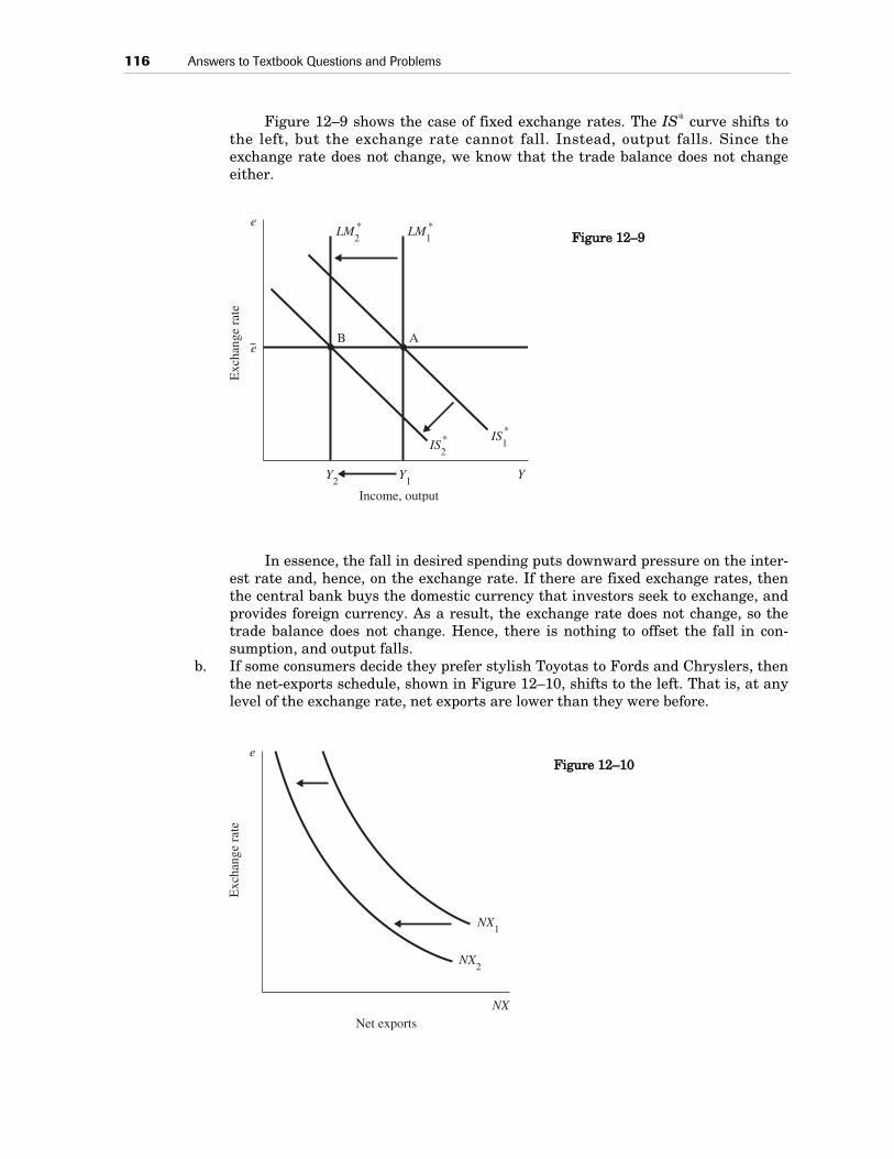
Figure 12–9 shows the case of fixed exchange rates. The IS* curve shifts tothe left, but the exchange rate cannot fall. Instead, output falls. Since theexchange rate does not change, we know that the trade balance does not changeeither.

In essence, the fall in desired spending puts downward pressure on the inter-est rate and, hence, on the exchange rate. If there are fixed exchange rates, thenthe central bank buys the domestic currency that investors seek to exchange, andprovides foreign currency. As a result, the exchange rate does not change, so thetrade balance does not change. Hence, there is nothing to offset the fall in con-sumption, and output falls.

b. If some consumers decide they prefer stylish Toyotas to Fords and Chryslers, thenthe net-exports schedule, shown in Figure 12–10, shifts to the left. That is, at anylevel of the exchange rate, net exports are lower than they were before.


e

e

Exc

hang

e ra

te

B A

Y

Income, output

Y1

IS2

IS1

LM2

LM1

* *

**

Y2


e

Exc

hang

e ra

te

NXNet exports

NX1

NX2


This shifts the IS* curve to the left as well, as shown in Figure 12–11 for the caseof floating exchange rates. Since the LM* curve is fixed, output does not change,while the exchange rate falls (depreciates).

The trade balance does not change either, despite the fall in the exchange rate. Weknow this since NX = S – I, and both saving and investment remain unchanged.

Figure 12–12 shows the case of fixed exchange rates. The leftward shift inthe IS* curve puts downward pressure on the exchange rate. The central bankbuys dollars and sells foreign exchange to keep e fixed: this reduces M and shiftsthe LM* curve to the left. As a result, output falls.

The trade balance falls, because the shift in the net exports schedule means thatnet exports are lower for any given level of the exchange rate.

c. The introduction of ATM machines reduces the demand for money. We know thatequilibrium in the money market requires that the supply of real balances M/Pmust equal demand:

M/P = L(r*, Y).A fall in money demand means that for unchanged income and interest rates, theright-hand side of this equation falls. Since M and P are both fixed, we know that


e

Exc

hang

e ra

te

A

B

YIncome, output

LM*

e1

e2

IS2

IS1

*

*


e

eExc

hang

e ra

te

B A

Y

Income, output

IS2

IS1

Y1

LM1

LM2

**

*

*

Y2


the left-hand side of this equation cannot adjust to restore equilibrium. We alsoknow that the interest rate is fixed at the level of the world interest rate. Thismeans that income—the only variable that can adjust—must rise in order toincrease the demand for money. That is, the LM* curve shifts to the right.

Figure 12–13 shows the case with floating exchange rates. Income rises, theexchange rate falls (depreciates), and the trade balance rises.

Figure 12–14 shows the case of fixed exchange rates. The LM* scheduleshifts to the right; as before, this tends to push domestic interest rates down andcause the currency to depreciate. However, the central bank buys dollars and sellsforeign currency in order to keep the exchange rate from falling. This reduces themoney supply and shifts the LM* schedule back to the left. The LM* curve contin-ues to shift back until the original equilibrium is restored.

In the end, income, the exchange rate, and the trade balance are unchanged.


e

Exc

hang

e ra

te

A

B

Y

Income, output

LM1

LM2

e2

e1

IS*

* *

Y1

Y2


e

e

Exc

hang

e ra

te

A

YIncome, output

LM*

IS*

Y1


2. a. The Mundell–Fleming model takes the world interest rate r* as an exogenousvariable. However, there is no reason to expect the world interest rate to be con-stant. In the closed-economy model of Chapter 3, the equilibrium of saving andinvestment determines the real interest rate. In an open economy in the long run,the world real interest rate is the rate that equilibrates world saving and worldinvestment demand. Anything that reduces world saving or increases worldinvestment demand increases the world interest rate. In addition, in the short runwith fixed prices, anything that increases the worldwide demand for goods orreduces the worldwide supply of money causes the world interest rate to rise.

b. Figure 12–15 shows the effect of an increase in the world interest rate under float-ing exchange rates. Both the IS* and the LM* curves shift. The IS* curve shifts tothe left, because the higher interest rate causes investment I(r*) to fall. The LM*

curve shifts to the right because the higher interest rate reduces money demand.Since the supply of real balances M/P is fixed, the higher interest rate leads to anexcess supply of real balances. To restore equilibrium in the money market,income must rise; this increases the demand for money until there is no longer anexcess supply.

We see from the figure that output rises and the exchange rate falls (depreciates).Hence, the trade balance increases.


e

Exc

hang

e ra

te

B

A

Y

Income, output

LM2

LM1

IS2

IS1

Y2

e2

e1

**

*

*

Y1


c. Figure 12–16 shows the effect of an increase in the world interest rate if exchangerates are fixed. Both the IS* and LM* curves shift. As in part (b), the IS* curveshifts to the left since the higher interest rate causes investment demand to fall.The LM* schedule, however, shifts to the left instead of to the right. This isbecause the downward pressure on the exchange rate causes the central bank tobuy dollars and sell foreign exchange. This reduces the supply of money M andshifts the LM* schedule to the left. The LM* curve must shift all the way back toLM in the figure, where the fixed-exchange-rate line crosses the new IS* curve.

In equilibrium, output falls while the exchange rate remains unchanged. Since theexchange rate does not change, neither does the trade balance.

3. a. A depreciation of the currency makes American goods more competitive. This isbecause a depreciation means that the same price in dollars translates into fewerunits of foreign currency. That is, in terms of foreign currency, American goodsbecome cheaper so that foreigners buy more of them. For example, suppose theexchange rate between yen and dollars falls from 200 yen/dollar to 100 yen/dollar.If an American can of tennis balls costs $2.50, its price in yen falls from 500 yen to250 yen. This fall in price increases the quantity of American-made tennis ballsdemanded in Japan. That is, American tennis balls are more competitive.


*2

e

e

Exc

hang

e ra

te

B A

Y

Income, output

LM2

LM1

IS1

IS2

* *

*

*

Y2

Y1


b. Consider first the case of floating exchange rates. We know that the position of theLM* curve determines output. Hence, we know that we want to keep the moneysupply fixed. As shown in Figure 12–17, we want to use fiscal policy to shift theIS* curve to the left to cause the exchange rate to fall (depreciate). We can do thisby reducing government spending or increasing taxes.

Now suppose that the exchange rate is fixed at some level. If we want toincrease competitiveness, we need to reduce the exchange rate; that is, we need tofix it at a lower level. The first step is to devalue the dollar, fixing the exchangerate at the desired lower level. This increases net exports and tends to increaseoutput, as shown in Figure 12–18. We can offset this rise in output with contrac-tionary fiscal policy that shifts the IS* curve to the left, as shown in the figure.


eE

xcha

nge

rate A

B

Y

Income, output

IS1

IS2

e1

e2

LM*

*

*

Y1

Income, output


e

Exc

hang

e ra

te A

C B

YYIncome, output

IS2

IS1

e2

e1

LM*

*

*


4. In the text, we assumed that net exports depend only on the exchange rate. This isanalogous to the usual story in microeconomics in which the demand for any good (inthis case, net exports) depends on the price of that good. The “price” of net exports isthe exchange rate. However, we also expect that the demand for any good depends onincome, and this may be true here as well: as income rises, we want to buy more of allgoods, both domestic and imported. Hence, as income rises, imports increase, so netexports fall. Thus, we can write net exports as a function of both the exchange rate andincome:

NX = NX(e, Y).Figure 12–19 shows the net exports schedule as a function of the exchange rate. Asbefore, the net exports schedule is downward sloping, so an increase in the exchangerate reduces net exports. We have drawn this schedule for a given level of income. Ifincome increases from Y1 to Y2, the net exports schedule shifts inward from NX(Y1) toNX(Y2).

a. Figure 12–20 shows the effect of a fiscal expansion under floating exchange rates.The fiscal expansion (an increase in government expenditure or a cut in taxes)shifts the IS* schedule to the right. But with floating exchange rates, if the LM*

curve does not change, neither does income. Since income does not change, thenet-exports schedule remains at its original level NX(Y1).


e

Exc

hang

e ra

te

NX

Net exports

NX (Y1)

NX (Y2)


e

Exc

hang

e ra

te

B

A

Income, outputIncome, output

IS1*

IS2*

LM*

e1

e2

Y1


The final result is that income does not change, and the exchange rate appreciatesfrom e1 to e2. Net exports fall because of the appreciation of the currency.

Thus, our answer is the same as that given in Table 12–1.b. Figure 12–21 shows the effect of a fiscal expansion under fixed exchange rates.

The fiscal expansion shifts the IS* curve to the right, from IS to IS . As in part(a), for unchanged real balances, this tends to push the exchange rate up. To pre-vent this appreciation, however, the central bank intervenes in currency markets,selling dollars and buying foreign exchange. This increases the money supply andshifts the LM* curve to the right, from LM to LM .

Output rises while the exchange rate remains fixed. Despite the unchangedexchange rate, the higher level of income reduces net exports because the net-exports schedule shifts inward.

Thus, our answer differs from the answer in Table 12–1 only in that underfixed exchange rates, a fiscal expansion reduces the trade balance.


e

Exc

hang

e ra

te A B

Y

Income, output

IS1*

IS2*

Y2

LM 2

LM 1

**

Y1

e

*2

*2

*1


*1

5. [Note the similarity to question 7 in Chapter 11.] We want to consider the effects of atax cut when the LM* curve depends on disposable income instead of income:

M/P = L[r, Y – T].A tax cut now shifts both the IS* and the LM* curves. Figure 12–22 shows the

case of floating exchange rates. The IS* curve shifts to the right, from IS to IS . TheLM* curve shifts to the left, however, from LM to LM .

We know that real balances M/P are fixed in the short run, while the interest rateis fixed at the level of the world interest rate r*. Disposable income is the only variablethat can adjust to bring the money market into equilibrium: hence, the LM* equationdetermines the level of disposable income. If taxes T fall, then income Y must also fallto keep disposable income fixed.

In Figure 12–22, we move from an original equilibrium at point A to a new equi-librium at point B. Income falls by the amount of the tax cut, and the exchange rateappreciates.


*1*

1*2

*2

e

Exc

hang

e ra

te

B

A

Y

Income, output

IS2*

IS1*

Y1

e2

e1

LM2

LM1

* *

Y2


If there are fixed exchange rates, the IS* curve still shifts to the right; but the ini-tial shift in the LM* curve no longer matters. That is, the upward pressure on theexchange rate causes the central bank to sell dollars and buy foreign exchange; thisincreases the money supply and shifts the LM* curve to the right, as shown in Figure12–23.

The new equilibrium, at point B, is at the intersection of the new IS* curve, IS , andthe horizontal line at the level of the fixed exchange rate. There is no differencebetween this case and the standard case where money demand depends on income.

6. Since people demand money balances in order to buy goods and services, it makes senseto think that the price level that is relevant is the price level of the goods and servicesthey buy. This includes both domestic and foreign goods. But the dollar price of foreigngoods depends on the exchange rate. For example, if the dollar rises from 100 yen/dollarto 150 yen/dollar, then a Japanese good that costs 300 yen falls in price from $3 to $2.Hence, we can write the condition for equilibrium in the money market as

M/P = L(r, Y),where

P = λPd + (1 – λ)Pf /e.


e

e

Exc

hang

e ra

te

A

B

Y

Income, output

LM1

LM2

IS2*

IS1*

Y1

Y2

* *

e

*2


a. A higher exchange rate makes foreign goods cheaper. To the extent that peopleconsume foreign goods (a fraction 1 – λ), this lowers the price level P that is rele-vant for the money market. This lower price level increases the supply of real bal-ances M/P. To keep the money market in equilibrium, we require income to riseto increase money demand as well.

Hence, the LM* curve is upward sloping.b. In the standard Mundell–Fleming model, expansionary fiscal policy has no effect

on output under floating exchange rates. As shown in Figure 12–24, this is nolonger true here. A cut in taxes or an increase in government spending shifts theIS* curve to the right, from IS to IS . Since the LM* curve is upward sloping, theresult is an increase in output.

c. A central assumption in this chapter is that the price level is fixed in the shortrun. That is, we assumed that the short-run aggregate supply curve is horizontalat P = P, as shown in Figure 12–25.


e

Exc

hang

e ra

te

A

B

Y

Income, output

IS1*

IS2*

e2

e1

LM*

Y1

Y2

*2

*1


P

P

Pric

e le

vel

YIncome, output


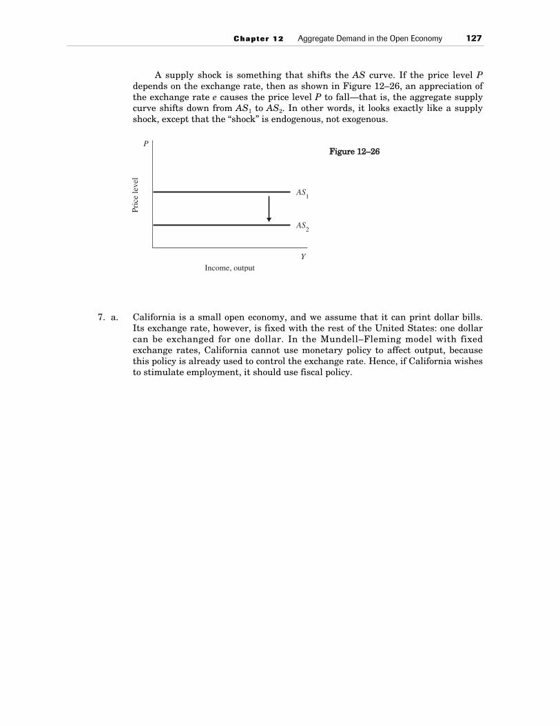
A supply shock is something that shifts the AS curve. If the price level Pdepends on the exchange rate, then as shown in Figure 12–26, an appreciation ofthe exchange rate e causes the price level P to fall—that is, the aggregate supplycurve shifts down from AS1 to AS2. In other words, it looks exactly like a supplyshock, except that the “shock” is endogenous, not exogenous.

7. a. California is a small open economy, and we assume that it can print dollar bills.Its exchange rate, however, is fixed with the rest of the United States: one dollarcan be exchanged for one dollar. In the Mundell–Fleming model with fixedexchange rates, California cannot use monetary policy to affect output, becausethis policy is already used to control the exchange rate. Hence, if California wishesto stimulate employment, it should use fiscal policy.


PPr

ice

leve

l

YIncome, output

AS1

AS2


b. In the short run, the import prohibition shifts the IS* curve out. This increasesdemand for Californian goods and puts upward pressure on the exchange rate. Tocounteract this, the Californian money supply increases, so the LM* curve shiftsout as well. The new short-run equilibrium is at point K in Figures 12–27(A) and(B).

Assuming that we started with the economy producing at its natural rate,the increase in demand for Californian goods tends to raise their prices. This risein the price level lowers real money balances, shifting the short-run AS curveupward and the LM* curve inward. Eventually, the Californian economy ends upat point C, with no change in output or the trade balance, but with a higher realexchange rate relative to Washington.


A. The Mundell-Fleming Model

B. The Model of Aggregate Supply and Aggregate Demand

∋

Exc

hang

e ra

tePr

ice

leve

l

A

C

P

P2

P1

AD1

AD2

K

Y

K

SRASA

C

Income, output

YIncome, output

LM*

IS*


MMoorree PPrroobblleemmss aanndd AApppplliiccaattiioonnss ttoo CChhaapptteerr 11221. a. Higher taxes shift the IS curve inward. To keep output unchanged, the central

bank must increase the money supply, shifting the LM curve to the right. At thenew equilibrium (point C in Figure 12–28), the interest rate is lower, the exchangerate has depreciated, and the trade balance has risen.


A. The IS–LM Model B. Net Foreign InvestmentLM1

LM2

IS2

IS1

NFI(r)

Income, outputY NFI

Rea

l int

eres

t rat

e

Exc

hang

e ra

te

A

C

r r

C. The Market for Foreign Exchange

Net exports

NX(e)

NFI

Net foreign investment

r2

r1

e2

NX2NX1

e1

e


NX(e)

b. Restricting the import of foreign cars shifts the NX(e) schedule outward [see panel(C)]. This has no effect on either the IS curve or the LM curve, however, becausethe NFI schedule is unaffected. Hence, output doesn’t change and there is no needfor any change in monetary policy. As shown in Figure 12–29, interest rates andthe trade balance don’t change, but the exchange rate appreciates.


A. The IS-LM Model B. Net Foreign Investment

LM

IS

NFI(r)

Income, outputY NFI

Rea

l int

eres

t rat

e

Exc

hang

e ra

te

r r


Net exports

NX(e)2

NX(e)1

NFI


e1

NX

e2

e


A. The IS–LM Model

2. a. The NFI curve becomes flatter, because a small change in the interest rate nowhas a larger effect on capital flows.

b. As argued in the text, a flatter NFI curve makes the IS curve flatter, as well.c. Figure 12–30 shows the effect of a shift in the LM curve for both a steep and a flat

IS curve. It is clear that the flatter the IS curve is, the less effect any change inthe money supply has on interest rates. Hence, the Fed has less control over theinterest rate when investors are more willing to substitute foreign and domesticassets.

d. It is clear from Figure 12–30 that the flatter the IS curve is, the greater effect anychange in the money supply has on output. Hence, the Fed has more control overoutput.


Rea

l int

eres

t rat

e

Y

LM1

ISsteep

ISflat

LM2

Cflat

Csteep

r

Income, output


3. a. No. It is impossible to raise investment without affecting income or the exchangerate just by using monetary and fiscal policies. Investment can only be increasedthrough a lower interest rate. Regardless of what policy is used to lower the inter-est rate (e.g., expansionary monetary policy and contractionary fiscal policy), netforeign investment will increase, lowering the exchange rate.

b. Yes. Policymakers can raise investment without affecting income or the exchangerate with a combination of expansionary monetary policy and contractionary fiscalpolicy, and protection against imports can raise investment without affecting theother variables. Both the monetary expansion and the fiscal contraction would putdownward pressure on interest rates and stimulate investment. It is necessary tocombine these two policies so that their effects on income exactly offset each other.The lower interest rates will, as in part (a), increase net foreign investment, whichwould normally put downward pressure on the exchange rate. The protectionistpolicies, however, shift the net-exports curve out; this puts countervailing upwardpressure on the exchange rate and offsets the effect of the fall in interest rates.Figure 12–31 shows this combination of policies.


LM

NX(e)

NX

Income, output

NFIY

NFI(r)I S

Net exports

v

rr

NFI

LM

I S

Y1, Y2

r1

r2

e

NX1 NX2

e1, e2

NFI1 NFI2

Net foreign in estment


c. Yes. Policymakers can raise investment without affecting income or the exchangerate through a home monetary expansion and fiscal contraction, combined with alower foreign interest rate either through a foreign monetary expansion or fiscalcontraction. The domestic policy lowers the interest rate, stimulating investment.The foreign policy shifts the NFI curve inward. Even with lower interest rates, thequantity of NFI would be unchanged and there would be no pressure on theexchange rate. This combination of policies is shown in Figure 12–32.

4. a. Figure 12–33 shows the effect of a fiscal contraction on a large open economy witha fixed exchange rate. The fiscal contraction shifts the IS curve to the left in panel


LM

NX(e)

NX

Income, output

NFIY

NFI(r)I S

Net exports

rr

NFI

Y1, Y2

r1

r2

e

e1, e2

NX1, NX2


NFI1, NFI2


(A), which puts downward pressure on the interest rate. This tends to increaseNFI and cause the exchange rate to depreciate [see panels (B) and (C)]. To avoidthis, the central bank intervenes and buys dollars. This keeps the exchange ratefrom depreciating; it also shifts the LM curve to the left. The new equilibrium, atpoint C, has an unchanged interest rate and exchange rate, but lower output.

This effect is the same as in a small open economy.


Income, outputY

C

NFI

NFI

A. The IS-LM Model

IS2

IS1

LM2LM1

Rea

l int

eres

t rat

e

rB. Net Foreign Investment

Exc

hang

e ra

te

r

Net exportsNX

NX(e)

e



A


b. A monetary expansion tends to shift the LM curve to the right, lowering the inter-est rate [panel (A) in Figure 12–34]. This tends to increase NFI and cause theexchange rate to depreciate [see panels (B) and (C)]. To avoid this depreciation,the central bank must buy its currency and sell foreign exchange. This reduces themoney supply and shifts the LM curve back to its original position. As in themodel of a small open economy, monetary policy is ineffectual under a fixedexchange rate.


Income, outputY NFI

NFI(r)

A. The IS-LM Model

IS

LM1

LM2

Rea

l int

eres

t rat

e

rB. Net Foreign Investment

Exc

hang

e ra

te

r

Net exportsNX

NX(e)

e




Documents

IS* curve to the left. If curve is unaffected. As shown in ...qed.econ.queensu.ca/pub/students/khans/ECON2450_AS4_SOL.pdf · the exchange rate floats freely, then the LM* curve is