Irregular Cellular Learning Automata

This article has been accepted for inclusion in a future issue of this journal. Content is final as presented, with the exception of pagination.

IEEE TRANSACTIONS ON CYBERNETICS 1

Irregular Cellular Learning AutomataMehdi Esnaashari and Mohammad Reza Meybodi

Abstract—Cellular learning automaton (CLA) is a recentlyintroduced model that combines cellular automaton (CA) andlearning automaton (LA). The basic idea of CLA is to use LAto adjust the state transition probability of stochastic CA. Thismodel has been used to solve problems in areas such as channelassignment in cellular networks, call admission control, imageprocessing, and very large scale integration placement. In thispaper, an extension of CLA called irregular CLA (ICLA) isintroduced. This extension is obtained by removing the structureregularity assumption in CLA. Irregularity in the structure ofICLA is needed in some applications, such as computer networks,web mining, and grid computing. The concept of expediency hasbeen introduced for ICLA and then, conditions under which anICLA becomes expedient are analytically found.

Index Terms—Expediency, irregular cellular learningautomata (ICLA), Markov process, steady-state analysis.

I. INTRODUCTION

CELLULAR automaton (CA) is a discrete model consistsof simple identical components, called cells, organized

into a regular grid structure. Each cell can assume a statefrom a finite set of states. The operation of a CA takes placein discrete steps according to a local rule, which depends onthe local environments of the cells. The local environment ofa cell is usually taken to be a small number of neighboringcells, which can include the cell itself [1]. The global stateof a CA, which represents the states of all its constitutingcells together, is referred to as a configuration. The local ruleand the initial configuration of a CA specify the evolution ofthat CA, which tells how each configuration is changed inone step. CA is particularly suitable for modeling natural sys-tems that can be described as massive collections of simpleobjects interacting locally with each other [2]. CA is calledcellular, because it is made up of cells like points in the lat-tice, and called automata, because it follows a simple localrule [3].

On the other hand, learning automaton (LA) is, by design,a simple agent for making simple and adaptive decisions inunknown random environments. Intuitively, LA could be con-sidered as a learning organism which tries different actions

Manuscript received November 9, 2013; revised June 16, 2014 andAugust 24, 2014; accepted August 26, 2014. This paper was recommendedby Associate Editor R. Selmic.

M. Esnaashari is with the Information Technology Department, IranTelecommunications Research Center, Tehran 1439955471, Iran (e-mail:[email protected]).

M. R. Meybodi is with the Computer Engineering and InformationTechnology Department, Amirkabir University of Technology, Tehran, Iranand also with the School of Computer Science, Institute for Studies inTheoretical Physics and Mathematics (IPM), Tehran 15914, Iran (e-mail:[email protected]).

Color versions of one or more of the figures in this paper are availableonline at http://ieeexplore.ieee.org.

Digital Object Identifier 10.1109/TCYB.2014.2356591

(from its action set) and selects new actions on the basis ofthe responses of the environment to previous actions. Oneattractive feature of this model is that it could be regardedas a simple unit from which complex structures could beconstructed. These could be designed to handle complicatedlearning problems [4]. In most applications, local interactionof LAs, which can be defined in a form of graph such astree, mesh, or array, is more suitable. In [5], CA and LAare combined, and a new model, which is called cellular LA(CLA), is obtained. This model, which opens a new learn-ing paradigm, is superior to CA because of its ability tolearn and is also superior to single LA because it consistsof a collection of LAs interacting with each other. CLA hasbeen used in many different applications including: channelassignment in cellular networks [6], call admission control incellular networks [7], and very large scale integration place-ment [8], to mention a few. In [11], a mathematical frameworkfor studying the behavior of the CLA has been introduced.It was shown that, for a class of rules called commutativerules, different models of CLA converge to a globally stablestate [7], [9]–[11].

In this paper, irregular CLA (ICLA) is introduced as anextension to CLA model, in which the structure regularityassumption is removed. We argue that in some applications,such as computer networks, web mining, and grid computing,problems could usually be described by graphs, with irregu-lar structures, and hence, an extension of CLA with irregularstructure is needed to model such problems.

For the proposed extended model, the concept of expediencyis introduced. Informally, an ICLA is said to be expedientif, in the long run, all of its constituting LA perform betterthan pure-chance automata. A pure-chance automaton is anautomaton which chooses any of its actions by pure chance.Expediency is a notion of learning. An automaton which iscapable of learning must do at least better than a pure-chanceautomaton [12]. The steady-state behavior of ICLA is studiedand then, conditions under which an ICLA becomes expedientare given.

The rest of this paper is organized as follows. In Section II,we briefly introduce CLA model. Sections III and IV presentICLA and its steady-state behavior, respectively. A set ofnumerical examples are given in Section V for illustrating thetheoretical results. In Section VI, we present a case study ofusing ICLA for problem solving in the area of wireless sensornetworks. Section VII is the conclusion.

II. CLA: COMBINATION OF CA AND LA MODELS

Before presenting CLA model in this section, we first givea brief introduction to CA and LA models.

2168-2267 c© 2014 IEEE. Personal use is permitted, but republication/redistribution requires IEEE permission.See http://www.ieee.org/publications_standards/publications/rights/index.html for more information.

mailto:[email protected]

mailto:[email protected]

http://ieeexplore.ieee.org

http://www.ieee.org/publications_standards/publications/rights/index.html


2 IEEE TRANSACTIONS ON CYBERNETICS

A. CA

A d-dimensional CA consists of an infinite d-dimensionallattice of identical cells. Each cell can assume a state from afinite set of states. The cells update their states synchronouslyon discrete steps according to a local rule. The new state ofeach cell depends on the previous states of a set of cells,including the cell itself, and constitutes its neighborhood. Thestates of all cells in the lattice are described by a configura-tion. A configuration can be described as the state of the wholelattice. The local rule and the initial configuration of CA spec-ify the evolution of CA, that is, how the configuration of CAevolves in time.

B. LA

LA is an abstract model which randomly selects one actionout of its finite set of actions and performs it on a randomenvironment. Environment then evaluates the selected actionand responses to the LA with a reinforcement signal. Basedon the selected action, and the received signal, LA updates itsinternal state and selects its next action.

Environment can be defined by the triple E = {α, β, c}where α = {α1, α2, . . . , αr} represents a finite input set,β = {β1, β2, . . . , βr} represents the output set, and c ={c1, c2, . . . , cr} is a set of penalty probabilities, where eachelement ci= E[β | α = αi] of c corresponds to one input αi. Anenvironment in which β assumes values in the interval [0, 1] isreferred to as an S-model environment. LAs are classified intofixed-structure stochastic, and variable-structure stochastic. Inthe following, we consider only variable-structure LAs.

A variable-structure LA is defined by the quadruple{α, β, p, T} in which α = {α1, α2, . . . , αr} represents theaction set of LA, β = {β1, β2, . . . , βr} represents the inputset, p = {p1, p2, . . . , pr} represents the action probability set,and finally p (k + 1) = T

[α (k), β (k), p (k)

]represents the

learning algorithm. This LA operates as follows. Based on theaction probability set p, LA randomly selects an action α (k),and performs it on the environment. After receiving the envi-ronment’s reinforcement signal (β (k)), LA updates its actionprobability set based on (1) or (2) according to the selectedaction α (k)

pi (k + 1) = pi (k) + β (k)[

br−1 − b · pi (k)

]

− [1 − β (k)] · a · pi (k) , when α (k) �= αi(1)

pi (k + 1) = pi (k) − β (k) · b · pi (k) + [1 − β (k)]·a · (1 − pi (k)) , when α (k) = αi.

(2)

In the above equations, a and b are reward and penaltyparameters respectively. For a = b, learning algorithm is calledLRP,1 for b << a it is called LRεP,2 and for b = 0, it is calledLRI .

3

Since its introduction in 1973 by Tsetlin [21], LA havebeen found a variety of applications in many different top-ics [22]–[25] and still appears in many recent researches suchas [26] and [27] to mention a few.

1Linear Reward-Penalty2Linear Reward epsilon Penalty3Linear Reward Inaction

C. CLA

A CLA is a CA in which a number of LAs is assigned toevery cell. Each LA residing in a particular cell determinesits action (state) on the basis of its action probability vector.Like CA, there is a local rule that CLA operates under. Thelocal rule of CLA and the actions selected by the neighboringLAs of any particular LA determine the reinforcement signalto that LA. The neighboring LAs (cells) of any particular LA(cell) constitute the local environment of that LA (cell). Thelocal environment of an LA (cell) is nonstationary due to thefact that the action probability vectors of the neighboring LAsvary during the evolution of CLA. The operation of a CLAcould be described as the following steps: At the first step,the internal state of every cell is determined on the basis ofthe action probability vector of the LA residing in that cell.In the second step, the local rule of CLA determines the rein-forcement signal to the LA residing in that cell. Finally, eachLA updates its action probability vector based on the suppliedreinforcement signal and the chosen action. This process con-tinues until the desired result is obtained. Formally, a CLAcan be defined as follows.

Definition 1: A d-dimensional CLA is a structure =(Zd, N,�, A,

), where as follows.

1) Zd is a lattice of d-tuples of integer numbers.2) N = {x1, x2,. . . , xm} is a finite subset of Zd called

neighborhood vector, where xi ∈ Zd.3) � is a finite set of states. The state of the cell ci is

denoted by ϕi.4) A is the set of LA each of which is assigned to one cell

of the CLA.5) Fi : ϕi → β is the local rule of the CLA in each cell ci,

where β is the set of values that the reinforcement signalcan take. It computes the reinforcement signal for eachLA based on the actions selected by the neighboring LA.

III. ICLA: EXTENSION TO CLA MODEL

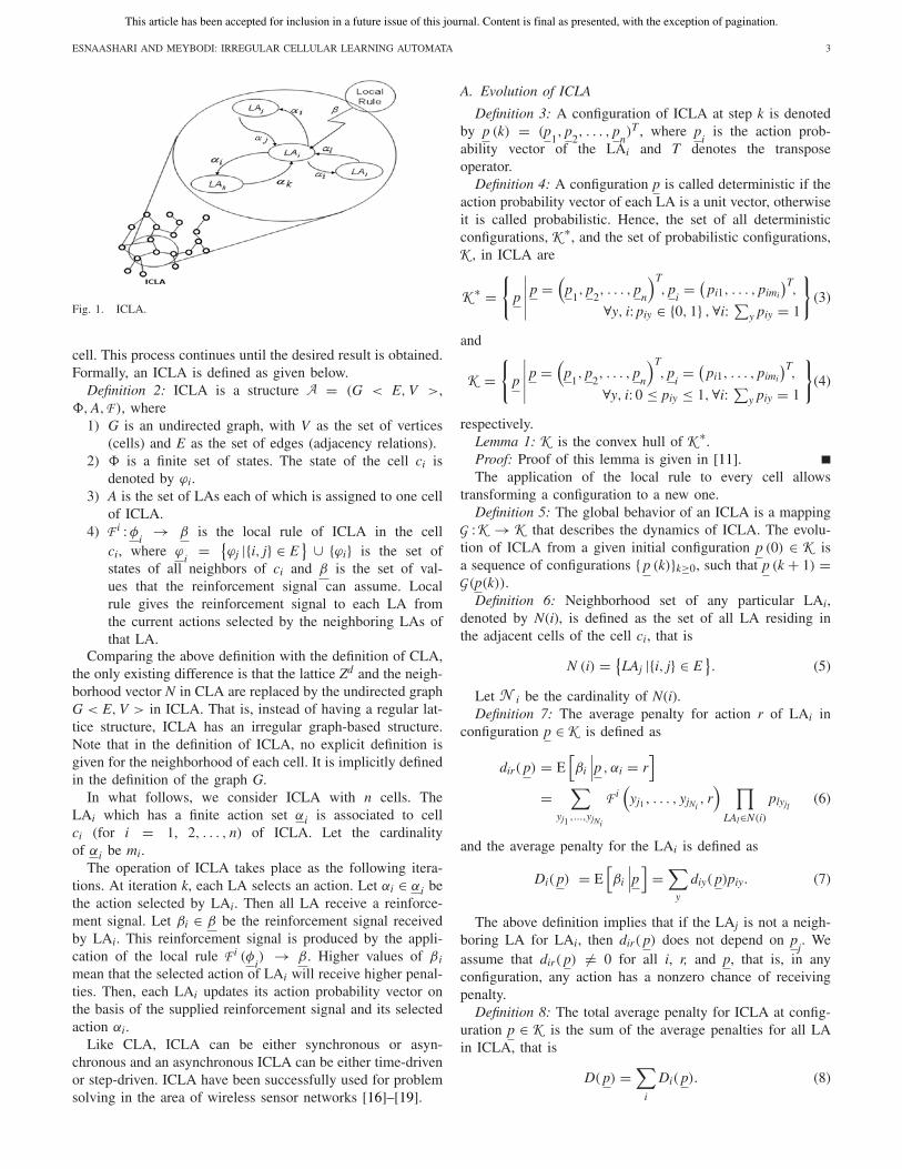
ICLA (Fig. 1) is a generalization of CLA in which therestriction of regular structure is removed. An ICLA is definedas an undirected graph in which, each vertex represents a celland is equipped with an LA, and each edge induces an adja-cency relation between two cells (two LAs). LA residing ina particular cell determines its state (action) according to itsaction probability vector. Like CLA, there is a rule that ICLAoperates under. The rule of ICLA and the actions selectedby the neighboring LAs of any particular LA determine thereinforcement signal to that LA. The neighboring LAs of anyparticular LA constitute the local environment of that LA. Thelocal environment of an LA is nonstationary because the actionprobability vectors of the neighboring LAs vary during theevolution of ICLA.

The operation of ICLA is similar to the operation of CLA.At the first step, the internal state of each cell is specified onthe basis of the action probability vector of the LA residing inthat cell. In the second step, the rule of ICLA determines thereinforcement signal to the LA residing in each cell. Finally,each LA updates its action probability vector on the basis ofthe supplied reinforcement signal and the internal state of the


ESNAASHARI AND MEYBODI: IRREGULAR CELLULAR LEARNING AUTOMATA 3

Fig. 1. ICLA.

cell. This process continues until the desired result is obtained.Formally, an ICLA is defined as given below.

Definition 2: ICLA is a structure = (G < E, V >,�, A, ), where

1) G is an undirected graph, with V as the set of vertices(cells) and E as the set of edges (adjacency relations).

2) � is a finite set of states. The state of the cell ci isdenoted by ϕi.

3) A is the set of LAs each of which is assigned to one cellof ICLA.

4) i : φi

→ β is the local rule of ICLA in the cellci, where ϕ

i= {

ϕj |{i, j} ∈ E} ∪ {ϕi} is the set of

states of all neighbors of ci and β is the set of val-ues that the reinforcement signal can assume. Localrule gives the reinforcement signal to each LA fromthe current actions selected by the neighboring LAs ofthat LA.

Comparing the above definition with the definition of CLA,the only existing difference is that the lattice Zd and the neigh-borhood vector N in CLA are replaced by the undirected graphG < E, V > in ICLA. That is, instead of having a regular lat-tice structure, ICLA has an irregular graph-based structure.Note that in the definition of ICLA, no explicit definition isgiven for the neighborhood of each cell. It is implicitly definedin the definition of the graph G.

In what follows, we consider ICLA with n cells. TheLAi which has a finite action set αi is associated to cellci (for i = 1, 2, . . . , n) of ICLA. Let the cardinalityof αi be mi.

The operation of ICLA takes place as the following itera-tions. At iteration k, each LA selects an action. Let αi ∈ αi bethe action selected by LAi. Then all LA receive a reinforce-ment signal. Let βi ∈ β be the reinforcement signal receivedby LAi. This reinforcement signal is produced by the appli-cation of the local rule i (φ

i) → β. Higher values of β i

mean that the selected action of LAi will receive higher penal-ties. Then, each LAi updates its action probability vector onthe basis of the supplied reinforcement signal and its selectedaction αi.

Like CLA, ICLA can be either synchronous or asyn-chronous and an asynchronous ICLA can be either time-drivenor step-driven. ICLA have been successfully used for problemsolving in the area of wireless sensor networks [16]–[19].

A. Evolution of ICLA

Definition 3: A configuration of ICLA at step k is denotedby p (k) = (p

1, p

2, . . . , p

n)T , where p

iis the action prob-

ability vector of the LAi and T denotes the transposeoperator.

Definition 4: A configuration p is called deterministic if theaction probability vector of each LA is a unit vector, otherwiseit is called probabilistic. Hence, the set of all deterministicconfigurations, ∗, and the set of probabilistic configurations,

, in ICLA are

∗ ={

p

∣∣∣∣∣p =

(p

1, p

2, . . . , p

n

)T, p

i= (

pi1, . . . , pimi

)T,

∀y, i: piy ∈ {0, 1} ,∀i:∑

y piy = 1

}

(3)

and

={

p

∣∣∣∣∣p =

(p

1, p

2, . . . , p

n

)T, p

i= (

pi1, . . . , pimi

)T,

∀y, i: 0 ≤ piy ≤ 1,∀i:∑

y piy = 1

}

(4)

respectively.Lemma 1: is the convex hull of ∗.Proof: Proof of this lemma is given in [11].The application of the local rule to every cell allows

transforming a configuration to a new one.Definition 5: The global behavior of an ICLA is a mapping: → that describes the dynamics of ICLA. The evolu-

tion of ICLA from a given initial configuration p (0) ∈ isa sequence of configurations { p (k)}k≥0, such that p (k + 1) =(p(k)).Definition 6: Neighborhood set of any particular LAi,

denoted by N(i), is defined as the set of all LA residing inthe adjacent cells of the cell ci, that is

N (i) = {LAj |{i, j} ∈ E

}. (5)

Let i be the cardinality of N(i).Definition 7: The average penalty for action r of LAi in

configuration p ∈ is defined as

dir( p) = E[βi

∣∣∣p , αi = r]

=∑

yj1 ,...,yjNi

i(

yj1 , . . . , yjNi, r

) ∏

LAl∈N(i)

plyjl(6)

and the average penalty for the LAi is defined as

Di( p) = E[βi

∣∣∣p]

=∑

y

diy( p)piy. (7)

The above definition implies that if the LAj is not a neigh-boring LA for LAi, then dir( p) does not depend on p

j. We

assume that dir( p) �= 0 for all i, r, and p, that is, in anyconfiguration, any action has a nonzero chance of receivingpenalty.

Definition 8: The total average penalty for ICLA at config-uration p ∈ is the sum of the average penalties for all LAin ICLA, that is

D( p) =∑

i

Di( p). (8)



IV. BEHAVIOR OF ICLA

In this section, we will study the asymptotic behavior of anICLA, in which all LA use the LRP learning algorithm [13],when operating within an S-model environment. We referto such an ICLA as ICLA with SLRP LA hereafter. Theprocess { p (k)}k≥0 which evolves according to the LRP learn-ing algorithm can be described by the following differenceequation:

p (k + 1) = p (k) + a · g(

p (k) , β (k))

(9)

where β (k) is composed of components β iy(k) (for 1 ≤ i ≤n, 1 ≤ y ≤ mi, and βiy1 = βiy2 for every y1, y2 such that1 ≤ y1, y2 ≤ mi), which are dependent on p (k). a is an n × ndiagonal matrix with aii = ai and ai represents the learningparameter for LAi. g represents the learning algorithm, whosecomponents can be obtained using LRP learning algorithm inS-model environment as follows:

gir

( pir, βir) ={

(1 − pir − βir) ; αi = r(βir

mi−1 − pir

); αi �= r

. (10)

From (9) it follows that { p (k)}k≥0 is a discrete-time Markovprocess [14] defined on the state space [given by (4)].Let

(,

)be a metric space, where d is the metric defined

according to(

p, q)

=∑

i

∥∥∥pi− q

i

∥∥∥ (11)

where∥∥X

∥∥ stands for the norm of the vector X.Lemmas 2 and 3, given below, state some properties of the

Markovian process given by (9).Lemma 2: The Markovian process given by (9) is strictly

distance diminishing.Proof: To prove this lemma, we will show that the

Markovian process given by (9) follows the definition of thestrictly distance diminishing processes given by Norman [15].The complete proof is given in Appendix A.

Corollary 1: Let p(h) denotes p (k + h) when p (k) = p and

q(h) denotes p (k + h) when p (k) = q. Then p(h) → q(h) ash → ∞ irrespective of the initial configurations p and q.

Proof: The proof is given in Appendix A.Lemma 3: The Markovian process given by (9) is ergodic.Proof : To prove the lemma we can see that the Markovian

process given by (9) has the following two properties.1) There are no absorbing states for { p (k)}, since there is

no p that satisfies p (k + 1) = p (k).2) The proposed process is strictly distance diminishing

(Lemma 2).From the above two properties and considering the results

given in corollary 1, we can conclude that the Markovianprocess { p (k)}k≥0 is ergodic.

Now define

�p (k) = E[p (k + 1)

∣∣∣p (k)

]− p (k). (12)

Since{

p (k)}

k≥0is Markovian and β (k) depends only on

p (k) and not on k explicitly, then �p (k) can be expressed as

a function of p (k). Hence we can write

�p = a f ( p). (13)

The components of �p can be obtained as follows:

�pir = aipir · [1 − pir − E [βir]

]

− ai

∑

y �=r

piy ·[

1

mi − 1E

[βiy

] − pir

]

= ai ·⎡

⎣ 1

mi − 1

∑

y �=r

piyE[βiy

] − pirE [βir]

⎤

⎦

= ai ·⎡

⎣ 1

mi − 1

∑

y �=r

piydiy( p) − pirdir( p)

⎤

⎦

= ai fir( p) (14)

where

fir( p) = 1

mi − 1

∑

y �=r

piydiy( p) − pirdir( p)

= 1

mi − 1

∑

y

piydiy( p) −(

1 + 1

mi − 1

)·[pirdir( p)

]

= 1

mi − 1·[Di( p) − mipirdir( p)

]. (15)

Lemma 4: Function f ( p) whose components are givenby (15) is Lipschitz continuous over the compact space .

Proof: Function f ( p) has compact support (it is definedover ), is bounded because −1 ≤ fir( p) ≤ 1 for allp, i, r, and is also continuously differentiable with respectto p over . Therefore, its first derivative with respect top is also bounded. Thus, using the Cauchy’s mean valuetheorem, it can be concluded that f ( p) is Lipschitz con-tinuous over the compact space with Lipschitz constantK = sup

p

∥∥∥∇pf ( p)

∥∥∥.

For different values of a, (9) generates different processesand we shall use pa (k) to denote this process whenever thevalue of a is to be specified explicitly. To find the approximat-ing ODE for the learning algorithm given by (9), we define asequence of continuous-time interpolation of (9), denoted bypa (t) and called an interpolated process, whose componentsare defined by

pai(t) = p

i(k), t ∈ [kai, (k + 1) ai) (16)

where ai is the learning parameter of the LRP algorithm forLAi. The interpolated process {pa (t)}t≥0 is a sequence of

random variables that takes values fromm1×...×mn , where

m1×...×mn is the space of all functions that, at each point, arecontinuous on the right and have a limit on the left over [0,∞)

and take values in , which is a bounded subset ofm1×...×mn .

Consider the following ordinary differential equation (ODE):

p = f ( p) (17)

where p is composed of the following components:

dpir

dt= 1


]. (18)



In the following theorem, we will show that (9) is theapproximation to the ODE (17). This means that if we havethe solution to (17), then we can obtain information regardingthe behavior of p (k).

Theorem 1: Using the learning algorithm (10) and consider-ing max

{a} → 0, p (k) is well approximated by the solution

of the ODE (17).Proof: Following conditions are satisfied by the learning

algorithm given by (10):1) { p (k)}k≥0 is a Markovian process.2) Given p (k), α (k) and β (k) are independent of α (k − 1)

and β (k − 1).3) f (p (k)) is independent of k.4) f (p (k)) is Lipshitz continuous over the compact space

(Lemma 4).5) E‖g( p) − f ( p)‖2 is bounded since g( p) ∈ [−1,

1]m1×...×mn .6) Learning parameters ai, i = 1, . . . , n are sufficiently small

since max{a} → 0.

Therefore, using [4, Th. A.1], we can conclude thetheorem.

Equation (9) is the so called Euler approximation to theODE (17). Specifically, if p (k) is a solution to (9) and p (t) isa solution to (17), then for any T > 0, we have

ai→00≤k≤T/ai

∥∥∥p

ir(k) − p (kai)

∥∥∥ = 0. (19)

What Theorem 1 says is that p (k), given by (9), will closelyfollow the solution of the ODE (17), that is, p (k) can be madeto closely approximate the solution of its approximating ODEby taking max

{a}

sufficiently small. Thus, if the ODE (17) hasa globally asymptotically stable equilibrium point, then we canconclude that (by taking max

{a}

sufficiently small), p (k), forlarge k, would be close to this equilibrium point irrespectiveof its initial configuration p (0). Therefore, the analysis of theprocess { p (k)}k≥0 is done in two stages. In the first stage, wesolve ODE (17) and in the second stage, we characterize thesolution of this ODE.

In the following subsections, we first find the equilibriumpoints of ODE (17), then study the stability property of theseequilibrium points, and finally state some theorems about theconvergence of ICLA.

A. Equilibrium Points

To find the equilibrium points of ODE (17), we first showthat this ODE has at least one equilibrium point and thenspecify a set of conditions which must be satisfied by aconfiguration p to be an equilibrium point of the ODE (17).

Lemma 5: ODE (17) has at least one equilibrium point.Proof: To prove this lemma, we first propose a continu-

ous mapping ζ( p) from to . Then, using the Brouwer’sfixed point theorem, we will show that any continuous map-ping from to has at least one fixed point. Finally, wewill show that the fixed point of ζ( p) is the equilibriumpoint of the ODE (17). This indicates that ODE (17) has atleast one equilibrium point. The complete proof is given inAppendix B.

Theorem 2: The equilibrium points of ODE (17) are theset of configurations p∗ which satisfy the set of conditionsp∗

ir = (∏

y �=r diy(p∗))/(∑

y1(∏

y2 �=y1diy2(p

∗))) for all i, r.Proof: To find the equilibrium points of ODE (17), we have

to solve equations of the form

dp∗ir (t)

dt= 0 for all i, r. (20)

Using (18), (20) can be rewritten as

1mi−1 ·

[Di

(p∗ (t)

)− mip∗

ir (t) dir

(p∗ (t)

)]= 0

for all i, r.(21)

These equations have solutions of the form

p∗ir =

Di

(p∗

)

midir

(p∗

) , for all i, r (22)

which after some algebraic manipulations, can be rewritten as

p∗ir =

∏y �=r diy

(p∗

)

∑y1

(∏y2 �=y1

diy2

(p∗

)) , for all i, r (23)

and hence the theorem.It follows from Theorem 2 that the difference equation given

by (13) has equilibrium points p∗ that satisfy the set of condi-tions p∗

ir (k) = (∏

y �=r diy(p∗ (k)))/(∑

y1(∏

y2 �=y1diy2(p

∗ (k))))for all i, r.

B. Stability Property

In this Section IV-B, we characterize the stability of equilib-rium configurations of ICLA, that is, the equilibrium points ofODE (17). To do this, the origin is first transferred to an equi-librium point p∗, and then a candidate for a Lyapunov functionis introduced for studying the stability of this equilibriumpoint. Consider the following transformation:

pir = pir −Di

(p∗

)

midir

(p∗

) for all i, r. (24)

Using this transformation, the origin is transferred to p∗.Lemma 6: Derivative of p with respect to time has compo-

nents of the following form:

dpir

dt= −dir( p)pir for all i, r. (25)

Proof: The proof is given in Appendix C.Corollary 2: p

irand its time derivative (dpir/dt) have

different signs.Proof: Considering the fact that dir( p) ≥ 0 for all configu-

rations p and for all i and r, the proof is an immediate resultof (25).

Theorem 3: A configuration p∗, whose components satisfyset of equations p∗

ir = (∏

y �=r diy(p∗))/(∑

y1(∏

y2 �=y1diy2(p

∗)))for all i, r, is an asymptotically stable equilibrium point ofODE (17) over .

Proof: To prove this theorem, we first apply transforma-tion (24) to transfer the origin to p∗. Then we propose



a positive definite function V( p) and show that the timederivative of V( p) is globally negative definite over .This indicates that p∗ is an asymptotically stable equilibriumpoint of ODE (17) over . The complete proof is given inAppendix D.

Corollary 3: The equilibrium point of ODE (17) is uniqueover .

Proof: Let p∗, q∗ be two equilibrium points of ODE (17).Theorem 3 proves that any equilibrium point of ODE (17),including p∗, is asymptotically stable over . This means thatall initial configurations within the state space converge top∗. Using a similar approach for q∗, one can conclude thatall initial configurations within the state space converge toq∗. This implies that p∗=q∗, and thus, the equilibrium point ofODE (17) is unique over .

C. Convergence Results

In this section, we summarize the main results specified inthe above lemmas and theorems in a main theorem (Theorem 4given below).

Theorem 4: An ICLA with SLRP LA, regardless of its initialconfiguration, converges in distribution to a random configu-ration, in which the mean value of the action probability ofany action of any LA is inversely proportional to the averagepenalty received by that action.

Proof: The evolution of an ICLA with SLRP LA is describedby (9). From this equation, it follows that { p (k)}k≥0 isa discrete-time Markov process. Lemma 3 states that thisMarkovian process is ergodic, and hence, it converges in dis-tribution to a random configuration p∗, irrespective of its initialconfiguration. Lemma 5 shows that such a configuration existsfor ICLA, Corollary 3 states that it is unique, and Theorem 3proves that it is asymptotically stable. Theorem 2 specifies theproperties of the configuration p∗. It shows that p∗ satisfies theset of conditions given by (22). According to (22), in config-uration p∗, the action probability of any action of any LA isinversely proportional to the average penalty received by thataction.

D. Expediency of ICLA

In this section, we introduce the concept of expediency forICLA and specify the set of conditions under which an ICLAbecomes expedient.

Definition 9: A pure-chance automaton is an automaton thatchooses each of its actions with equal probability i.e., by purechance, that is, an m-action automaton is pure-chance if pi =(1/m), i = 1, 2, . . . , m.

Definition 10: A pure-chance ICLA is an ICLA, for whichevery cell contains a pure-chance automaton rather than aLA. The configuration of a pure-chance ICLA is denotedby ppc.

Definition 11: An ICLA is said to be expedient with respectto the cell ci if

k→∞ p (k) = p∗ exists and the following

inequality holds:

k→∞ E[Di

(p (k)

)]<

1

mi

∑

y

diy

(p∗). (26)

TABLE ISPECIFICATIONS USED FOR NUMERICAL EXAMPLE 1

In other words, an ICLA is expedient with respect to thecell ci if, in the long run, the ith LA performs better (receivesless penalty) than a pure-chance automaton.

Definition 12: An ICLA is said to be expedient if it isexpedient with respect to every cell in ICLA.

Theorem 5: An ICLA with SLRP LA, regardless of the localrule being used, is expedient.

Proof: To prove this theorem, we show that an ICLA withSLRP LA is expedient with respect to every cell in ICLA. Theproof is given in Appendix E.

V. NUMERICAL EXAMPLES

In this section, we will give a number of numerical exam-ples for illustrating the analytical results specified in previoussections. The first two sets of examples are used to illustratethe analytical results given in Theorem 4, and the next set ofexamples is used to study the behavior of ICLA in terms ofexpediency.

A. Numerical Example 1

This set of examples are given to illustrate that the actionprobability of any action of any LA in an ICLA with SLRP LAconverges in distribution to a random variable, whose meanis inversely proportional to the average penalty received bythat action. We consider three different ICLAs with differentnumber of cells and different number of cell states. Table Igives the specifications used for this set of simulations. Here,ICLA(n,m) refers to an ICLA with n cells and m states for eachcell. Table II compares the action probabilities of the actionsof the LA in each ICLA at the end of the simulation time(k > 3 × 106) with their theoretical values obtained from (22).As it can be seen from these tables, the action probabilitiesof all actions and their theoretical values approach each other.This is in coincidence with the results of the theoretical anal-ysis given in Theorem 4, that is, an ICLA with SLRP LAconverges in distribution to a random configuration, in whichthe mean value of the action probability of any action of anyLA is inversely proportional to the average penalty receivedby that action. Fig. 2 also shows the approach of these twovalues to each other over the simulation time for randomlyselected actions of three randomly selected LA from ICLA2,3and ICLA5,5.

B. Numerical Example 2

The goal of conducting this set of numerical examplesis to study the convergence behavior of ICLA when itstarts to evolve within the environment from different initialconfigurations. For this paper, we use an ICLA5,5 with SLRP



TABLE IIRESULTS OF THE NUMERICAL EXAMPLE 1 FOR ICLA2,3, ICLA3,2, ICLA5,5 ( pij IS THE ACTION PROBABILITY OF THE jTH ACTION OF THE iTH LA

OBTAINED FROM THE SIMULATION STUDY AND p∗ij IS THE CORRESPONDING THEORETICAL VALUE)

Fig. 2. Results of the numerical example 1 for randomly selected actions oftwo randomly selected LA from ICLA2,3, ICLA5,5.

LA. Table III gives the initial configurations of this ICLA. Inthis table, for each configuration, the initial action probabil-ity vectors for LA are given from left to right. For example,in configuration 3, the initial action probability vector of theLA4 is [0.5, 0.1, 0.1, 0.2, 0.1]T . Fig. 3 plots the evolution

TABLE IIIINITIAL CONFIGURATIONS FOR ICLA5,5 USED IN

NUMERICAL EXAMPLE 2

of the action probabilities of two randomly selected actionsfrom two of the LA in ICLA for different initial configura-tions. As it can be seen from this figure, no matter what theinitial configuration of ICLA is, it converges to its equilibriumconfiguration. Thus, the results of this set of examples coin-cide with the results given in Theorem 4 in Section III, thatis, the convergence of ICLA to its equilibrium configurationis independent of its initial configuration.

C. Numerical Example 3

This set of numerical examples is conducted to studythe behavior of ICLA in terms of the expediency. For this



Fig. 3. Results of the numerical example 2 for randomly selected actions oftwo randomly selected LA.

TABLE IVRESULTS OF THE NUMERICAL EXAMPLE 3

paper, we use the specifications of the first numerical exam-ple, given in Table I. Table IV compares E[Di(p(k))] and(1)/(mi)

∑y diy(p(k)) at the end of the simulation time (k >

2.85 × 106) for all LA of all ICLAs given in Table I. As itcan be seen from this table, the average penalty received byany LA is less than that of a pure chance automaton. This isin coincidence with the theoretical results given in Theorem 5,i.e., an ICLA with SLRP LA, regardless of the local rule beingused, is expedient.

VI. CASE STUDY

To demonstrate the superiority of ICLA over LA, in thissection we compare the results of applying these two modelsfor solving the dynamic point coverage problem [20] in thearea of wireless sensor networks. In this problem, an unknownnumber of targets are moving throughout the sensor field and

Fig. 4. Comparison of LA and ICLA for solving dynamic point coverageproblem in terms of (a) network detection rate (ηD) and (b) network redundantactive rate (ηR) criteria.

the aim is to detect and track these moving targets using asfew sensor nodes as possible.

We have proposed two different approaches for solving thisproblem: 1) by using a number of noncooperating LA, oneat each sensor node of the network [20] and 2) by using anICLA, in which there again exists one LA at each sensor node,but these LA cooperate with each other [18]. Fig. 4 comparesthe results of these two approaches in terms of the followingtwo criteria.

1) Network Detection Rate (ηD): This criterion determinesthe accuracy of detecting and tracking moving targets.

2) Network Redundant Active Rate (ηR): This criteriondetermines the ratio of the time that a target is redun-dantly detected by more than one sensor node.

As it can be seen from this figure, using ICLA, results inhigher ηD and lower ηR than using LA. In other words, theaim of the network, which is to detect moving targets (ηD)using as few sensor nodes as possible (ηR), is better fulfilledwhen LA residing in different nodes of the network cooperatewith each other.

VII. CONCLUSION

In this paper, we proposed ICLA as an extension to CLAmodel. In contrast to CLA, the proposed model have irregularstructure which is needed for modeling problems in some areassuch as computer networks, web mining, and grid computing.The steady-state behavior of the proposed model was ana-lytically studied and the results of this paper were illustratedthrough some numerical examples. The concept of expediencywas introduced for the proposed learning model. An ICLAis expedient with respect to each of its cells if, in the longrun, the LA resides in that cell performs better (receives lesspenalty) than a pure-chance automaton. An ICLA is expedient,



if it is expedient with respect to all of its constituting cells.Expediency is a notion of learning. Any model that is saidto learn must then do at least better than its equivalent pure-chance model. The intended analytical studies showed that theproposed model, using SLRP learning algorithm, is expedient.The proposed analytical results are valid only if the learningrate is sufficiently small.

APPENDIX A

Proof of Lemma 2: Let ES = {α|α = (αT1 , αT

1 , . . . , αTn )T}

be the event set which causes the evolution of the state p (k) .

The evolution of the state p (k) is dependent on the occurrenceof an associated event ES(k). Thus

p (k + 1) = fES(k)

(p (k)

)(27)

where fES(k) is defined according to (9). Let Pr [ES(k) =e|p(k) = p] = φe( p) where φe( p) is a real-valued function

on ES × . Now define m (φe) and μ (fe) as

m (φe) = supp�=p′

∣∣∣φe( p) − φe

(p′

)∣∣∣(

p, p′) (28)

μ ( fe) = supp�=p′

(fe( p), fe

(p′

))

(p, p′

) (29)

and

μ (fe) = supp �=p′

(fe( p), fe

(p′

))

(p, p′

) (30)

whether or not these are finite. The following propositions areheld.

1) ES is a finite set.2)

(,

)is a metric space and is compact.

3) m (φe) < ∞ for all e ∈ ES4) μ (fe) < 1 for all e ∈ ES. To see this, consider p and q

as two states of the process { p(k)}.From (10) and (11) we have

μ ( fe) =(

fe( p), fe(

q))

(p, q

) =∑

i

∥∥∥fei

(p

i

)− fei

(q

i

)∥∥∥∑

i

∥∥∥pi− q

i

∥∥∥

=∑

i (1 − ai) ·∥∥∥p

i− q

i

∥∥∥

∑i

∥∥∥p

i− q

i

∥∥∥

. (31)

Since 0 < ai < 1,∀i it follows that μ (fe) < 1.Therefore, and according to the definition of the distance

diminishing processes given by Norman [15], Markovianprocess given by (9) is strictly distance diminishing.

Proof of Corollary 1: From Lemma 2, It follows that:(

p(h), q(h))

=∑

i

(1 − ai)h ·

∥∥∥pi− q

i

∥∥∥. (32)

Right hand side of (32) tends to zero as h → ∞. Hencep(h) → q(h) irrespective of the initial configurations p and q.

APPENDIX B

Proof of Lemma 5: Let ζ( p) = af ( p) + p where matrix ais equivalent to the one given in (9). Components of ζ( p) canbe obtained as follows:

ζir( p) = ai


]+ pir. (33)

It is easy to verify that 0 ≤ ζir( p) < 1 for all i and r. Thus,ζ( p) is a continuous mapping from to . Since is closed,bounded, and convex (Lemma 1), we can use the Brouwer’sfixed point theorem to show that ζ( p) has at least one fixedpoint. Let p∗ be a fixed point of ζ( p), thus we have

ζ(

p∗) = p∗ (34)

or equivalently

a f(

p∗) + p∗ = p∗. (35)

Since a is a diagonal matrix with no zero elements on itsmain diagonal, it can be concluded from (35) that

f(

p∗) = 0. (36)

Since every point p∗, that satisfies f (p∗) = 0, is an equilib-rium point of ODE (17), we can conclude that ODE (17) hasat least one equilibrium point.

APPENDIX C

Proof of Lemma 6: Let

δ∗ir =

Di

(p∗

)

midir

(p∗

). (37)

Using (24) and (37), components of the derivative of p withrespect to time can be given as

dpir

dt= dpir

dt+ dδ∗

ir

dt= dpir

dtfor all i, r. (38)

Using (18) and (37), (38) can be rewritten as

dpir

dt= 1

mi − 1·[Di( p) − mi · (

pir + δ∗ir

) · dir( p)]. (39)

Equation (39) is valid for all configurations p including qin which qir = 0 for a particular action r of the ith LA. Forthis configuration, it is easy to verify that (dq

ir)/(dt) = 0.

Next, use (7) to rewrite (39) as follows:

dpirdt = 1

mi−1 ·[

dir( p) · (1 − mi) · (pir + δ∗

ir

)+∑

y �=r

(piy + δ∗

iy

)diy( p)

]

for all i, r.

(40)

Equation (40) is also valid for all configurations p includingq. Thus, we have

dqir

dt= 1

mi − 1·⎡

⎣dir

(q)

· (1 − mi) · δ∗ir+

∑y �=r

(qiy + δ∗

iy

)diy

(q)

⎤

⎦ = 0 (41)

from which it immediately follows that:

dir

(q)

· (1 − mi) · δ∗ir +

∑

y �=r

(qiy + δ∗

iy

)diy

(q)

= 0. (42)



Since none of the terms in (42) depend on the value of qir,this equation is valid for all configurations p, that is

dir( p) · (1 − mi) · δ∗ir+∑

y �=r

(piy + δ∗

iy

)diy( p) = 0, for all p, i, r.

(43)

Using (43) in (40) we get

dpir

dt= −dir( p)pir for all i, r (44)

and hence the lemma.

APPENDIX D

Proof of Theorem 3: Apply transformation (24) to transferthe origin to p∗. Now consider the following positive definiteLyapunov function:

V(

p)

= −∑

i

∑

y

piy · ln(1 − piy

). (45)

V(p) ≥ 0 for all configurations p and is zero only whenpir = 0 for all i and r. Time derivative of V(.) can beexpressed as

V(

p)

= −∑

i

∑

y

dpiy

dt· υ

(piy

)(46)

where

υ(piy

) =[

ln(1 − piy

) · (1 − piy

) − piy

1 − piy

]

. (47)

Considering the value of piy

, following three cases may arisefor each term of this derivative.

1) 0 < piy ≤ 1: In this case, υ(piy

)< 0 and (dpiy)/(dt) <

0 (Corollary 2). Therefore, (dpiy)/(dt) · υ(piy

)> 0.

2) −1 ≤ piy < 0: In this case, υ(piy

)> 0 and (dpiy)/(dt)

> 0 (Corollary 2). Therefore, (dpiy)/(dt) · υ(piy

)> 0.

3) piy = 0: In this case, (dpiy)/(dt) · υ(piy

)= 0.

Thus, V(p) ≤ 0, for all configurations p and is zeroonly when pir = 0 for all i and r. Therefore, using theLyapunov theorems for autonomous systems, it can be provedthat p∗ is an asymptotically stable equilibrium point ofODE (17) over .

APPENDIX E

Proof of Theorem 5: We have to show that an ICLA withSLRP LA is expedient with respect to all of its cells; that is,

k→∞ p (k) = p∗ exists and the following inequality holds:

k→∞ E[Di

(p (k)

)]<

1

mi

∑

y

diy

(p∗), for every i. (48)

Using (7), the left hand side of this inequality can berewritten as

limk→∞ E

[Di

(p (k)

)]= lim

k→∞ E

⎡

⎣∑

y

diy

(p (k)

)piy (k)

⎤

⎦

=∑

y

limk→∞ E

[diy

(p (k)

)piy (k)

]. (49)

Since diy

(p (k)

)and piy (k) are independent, (49) can be

simplified to

limk→∞ E

[Di

(p (k)

)]

=∑

y

(lim

k→∞ E[diy

(p (k)

)]· lim

k→∞ E[piy (k)

]). (50)

From Theorem 4, we have limk→∞ E[p(k)] = p∗ and

hence limk→∞ E

[pir (k)

] = p∗ir for all i and r. Using (6),

limk→∞ E[dir(p(k))] can be computed as follows:

k→∞ E[dir

(p (k)

)]=

k→∞

E

⎡

⎣∑

yj1 ,...,yjNi

Fi(

yj1 , yj2 , . . . , yjNi, r

) ∏

LAl∈N(i)

plyjl(k)

⎤

⎦

=∑

yj1 ,...,yjNi

Fi(

yj1 , yj2 , . . . , yjNi, r

)

∏

LAl∈N(i)k→∞ E

[plyjl

(k)]

= dir

(p∗ (k)

). (51)

Thus, we get

limk→∞ E

[Di

(p (k)

)]=

∑

y

(diy

(p∗) p∗

iy

). (52)

Now, we have to show that∑

y

diy

(p∗) p∗

iy <1

mi

∑

y

diy

(p∗) for every i. (53)

Each side of this inequality is a convex combination ofdiy(p∗), y = 1, . . . , mi. In the convex combination given onthe right hand side of (53), weights of all dir(p∗) are equal to(1)/(mi), whereas in the convex combination given on the lefthand side, weight of each dir(p∗) is inversely proportional toits value, that is, the larger dir(p∗), the smaller its weight is[considering (22)]. Therefore, the convex combination givenon the left hand side of inequality (53) is smaller than the onegiven on the right hand side, and hence the theorem.

REFERENCES

[1] J. Kari, “Reversibility of 2D cellular automata is undecidable,” Phys. D,vol. 45, nos. 1–3, pp. 379–385, 1990.

[2] N. H. Pakard and S. Wolfram, “Two-dimensional cellular automata,”J. State Phys., vol. 38, nos. 5–6, pp. 901–946, 1985.

[3] E. Fredkin, “Digital machine: An informational process based onreversible cellular automata,” Phys. D, vol. 45, nos. 1–3, pp. 254–270,1990.

[4] M. A. L. Thathachar and P. S. Sastry, Networks of Learning Automata.Boston, MA, USA: Kluwer Academic, 2004.

[5] M. R. Meybodi, H. Beigy, and M. Taherkhani, “Cellular learningautomata and its applications,” Sharif J. Sci. Technol., vol. 19, no. 25,pp. 54–77, 2003.

[6] H. Beigy and M. R. Meybodi, “A self-organizing channel assignmentalgorithm: A cellular learning automata approach,” in Intelligent DataEngineering and Automated Learning, vol. 2690. New York, NY, USA:Springer, 2003, pp. 119–126.

[7] H. Beigy and M. R. Meybodi, “Asynchronous cellular learningautomata,” Automatica, vol. 44, no. 5, pp. 1350–1357, 2008.



[8] M. R. Meybodi and F. Mehdipour, “Application of cellular learn-ing automata with input to VLSI placement,” J. Modarres, vol. 16,pp. 81–95, 2004.

[9] H. Beigy and M. R. Meybodi, “Open synchronous cellular learningautomata,” Adv. Complex Syst., vol. 10, no. 4, pp. 527–556, 2007.

[10] H. Beigy and M. R. Meybodi, “Cellular learning automata with multiplelearning automata in each cell and its applications,” IEEE Trans. Syst.,Man, Cybern. B, Cybern., vol. 40, no. 1, pp. 54–66, Feb. 2010.

[11] H. Beigy and M. R. Meybodi, “A mathematical framework for cellularlearning automata,” Adv. Complex Syst., vol. 7, no. 3, pp. 295–320, 2004.

[12] M. L. Tsetlin, “On the behavior of finite automata in random media,”Autom. Remote Control, vol. 22, no. 10, pp. 1210–1219, 1962.

[13] K. S. Narendra and M. A. L. Thathachar, Learning Automata: AnIntroduction. Englewood Cliffs, NJ, USA: Prentice-Hall, 1989.

[14] D. L. Isaacson and R. W. Madsen, Markov Chains: Theory andApplications. New York, NY, USA: Wiley, 1976.

[15] M. F. Norman, “Some convergence theorems for stochastic learningmodels with distance diminishing operators,” J. Math. Psychol., vol. 5,no. 1, pp. 61–101, 1968.

[16] M. Esnaashari and M. R. Meybodi, “Irregular cellular learning automataand its application to clustering in sensor networks,” in Proc. 15th Conf.Elect. Eng., Telecommunication Research Center, Tehran, Iran, 2007.

[17] M. Esnaashari and M. R. Meybodi, “A cellular learning automata basedclustering algorithm for wireless sensor networks,” Sens. Lett., vol. 6,no. 5, pp. 723–735, 2008.

[18] M. Esnaashari and M. R. Meybodi, “Dynamic point coverage problemin wireless sensor networks: A cellular learning automata approach,”J. Ad hoc Sens. Wireless. Netw., vol. 10, nos. 2–3, pp. 193–234, 2010.

[19] M. Ahmadinia, M. R. Meybodi, M. Esnaashari, and H. AlinejadRokney, “Energy efficient and multi clustering algorithm in wirelessnetworks using cellular learning automata,” IETE J. Res., vol. 59, no. 6,pp. 774–782, 2013.

[20] M. Esnaashari and M. R. Meybodi, “A learning automata based schedul-ing solution to the dynamic point coverage problem in wireless sensornetworks,” Comput. Netw., vol. 54, no. 14, pp. 2410–2438, 2010.

[21] M. L. Tsetlin, “Automaton theory and modeling of biological systems,”New York, NY, USA: Academic Press, 1973.

[22] A. G. Barto and P. Anandan, “Pattern-recognizing stochastic learningautomata,” IEEE Trans. Syst., Man, Cybern. B, Cybern., vol. 15, no. 3,pp. 360–375, May/Jun. 1985.

[23] K. S. Narendra and K. Parthasarathy, “Learning automata approach tohierarchical multi-objective analysis,” IEEE Trans. Syst., Man, Cybern.B, Cybern., vol. 21, no. 1, pp. 263–272, Jan./Feb. 1991.

[24] P. S. Sastry, V. V. Phansalkar, and M. Thathachar, “Decentralized learn-ing of nash equilibria in multi-person stochastic games with incompleteinformation,” IEEE Trans. Syst., Man, Cybern. B, Cybern., vol. 24, no. 5,pp. 769–777, May 1994.

[25] O.-C. Granmo, B. J. Oommen, S. A. Myrer, and M. G. Olsen, “Learningautomata-based solutions to the nonlinear fractional knapsack problemwith applications to optimal resource allocation,” IEEE Trans. Syst.,Man, Cybern. B, Cybern., vol. 37, no. 2, pp. 166–175, Feb. 2007.

[26] B. J. Oommen and K. Hashem, “Modeling the “learning process” ofthe teacher in a tutorial-like system using learning automata,” IEEETrans. Syst., Man, Cybern. B, Cybern., vol. 43, no. 6, pp. 2020–2031,Dec. 2013.

[27] A. Yazidi, O.-C. Granmo, and B. J. Oommen, “Learning automatonbased on-line discovery and tracking of spatio-temporal event patterns,”IEEE Trans. Cybern., vol. 43, no. 3, pp. 1118–1130, Jun. 2013.

Mehdi Esnaashari received the B.S., M.S., andthe Ph.D. degrees in computer engineering from theAmirkabir University of Technology, Tehran, Iran,in 2002, 2005, and 2011, respectively.

He is currently an Assistant Professor with IranTelecommunications Research Center, Tehran. Hiscurrent research interests include computer net-works, learning systems, soft computing, and infor-mation retrieval.

Mohammad Reza Meybodi received the B.S. andM.S. degrees in economics from Shahid BeheshtiUniversity, Tehran, Iran, in 1973 and 1977, respec-tively, and the M.S. and Ph.D. degrees in computerscience from Oklahoma University, Norman, OK,USA, in 1980 and 1983, respectively.

He is currently a Full Professor with ComputerEngineering Department, Amirkabir University ofTechnology, Tehran. Prior to his current posi-tion, he was an Assistant Professor with WesternMichigan University, Kalamazoo, MI, USA, from

1983 to 1985, and an Associate Professor with Ohio University, Athens,OH, USA, from 1985 to 1991. His current research interests include channelmanagement in cellular networks, learning systems, parallel algorithms, softcomputing, and software development.

Documents

Irregular Cellular Learning Automata