IRON LOSS CALCULATION OF AN INTERNAL PERMANENT …...IRON LOSS CALCULATION OF AN INTERNAL PERMANENT MAGNET SYNCHRONOUS MACHINE FOR A FUEL CELL CAR Electric Drive System Research Activities

Technik und Informatik / Wissens- und Technologietransfer

IRON LOSS CALCULATION OF AN INTERNALPERMANENT MAGNET SYNCHRONOUSMACHINE FOR A FUEL CELL CAR

Electric Drive System Research Activities at Bern University of Applied SciencesEngineering and Information Technology

Prof. Andrea Vezzini, SwitzerlandDr. sc. techn. ETHZ

easc-2009, July 7th 2009

1


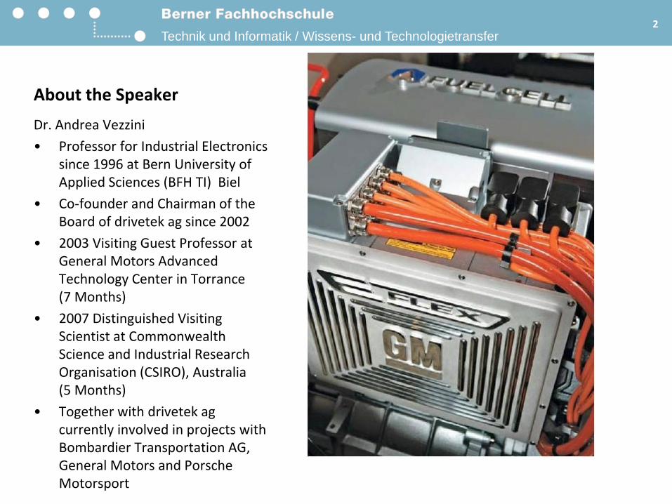
About the Speaker

Dr. Andrea Vezzini

• Professor for Industrial Electronics since 1996 at Bern University of Applied Sciences (BFH TI) Biel

• Co-founder and Chairman of the Board of drivetek ag since 2002

• 2003 Visiting Guest Professor at General Motors Advanced Technology Center in Torrance (7 Months)

• 2007 Distinguished Visiting Scientist at Commonwealth Science and Industrial Research Organisation (CSIRO), Australia (5 Months)

• Together with drivetek agcurrently involved in projects with Bombardier Transportation AG, General Motors and Porsche Motorsport

2


BFH Engineering and Information Technology

• Established in 1890

• Since 1998 Part of Bern University of Applied Sciences

• 6 Divisions with a total of 1’300 students, second biggest in Switzerland

• External Turnover withaR&D 2008:approx. 8 Mio. CHF(+ 2.5 Mio. CHF internal funding)

• Strategic Programs in Fuel Cell Development, Automotive Systems and Renewable Energy

• Over 10 Innovation prices since 1993

3


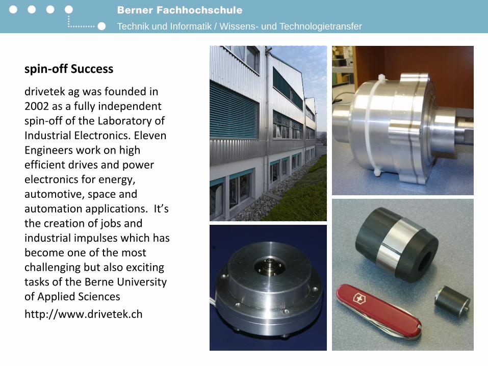
spin-off Success

drivetek ag was founded in 2002 as a fully independent spin-off of the Laboratory of Industrial Electronics. Eleven Engineers work on high efficient drives and power electronics for energy, automotive, space and automation applications. It’s the creation of jobs and industrial impulses which has become one of the most challenging but also exciting tasks of the Berne University of Applied Sciences

http://www.drivetek.ch


Content

• Internal Permanent Magnet Synchronous Motor Fundamentals

• Design Flow

• Core Loss Calculations

• Examples

“The outcome of any serious research can only be to make two questions grow where only one grew before.”

Thorstein VeblenUS economist & social philosopher (1857 - 1929)

5


Types of PM Synchronous Motors

• The amount of PM-generated magnetic flux linked by the coils of the stator remains fixed.

• As a result, the back-electromotive force (back-emf) voltage induced by the PMs increases linearly with the speed of the rotor.

• As the rotor speed increases the back-emf voltage rises, which results in a rapid reduction in the available voltage, (the difference between the supply voltage and the back-emf). When there is no longer any voltage available to drive current into the stator, the maximum speed has been reached.

• Depending on the rotor geometry, PM Synchronous show different torque-speed behavior.

6

a) Surface PermanentMagnet Motor

b) Inset Permanent Magnet Motor

c) V-Shaped Single Layer IPM

d) V-Shaped Double Layer IPM

e) U-Shaped Double Layer IPM

a)

d) e)

c)

b)


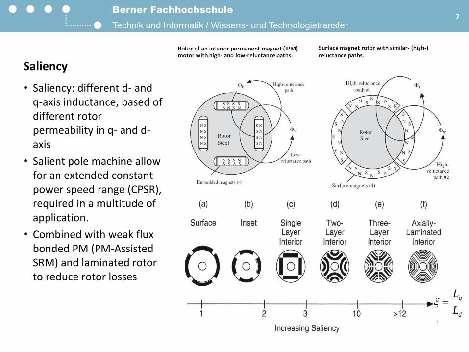
Saliency

• Saliency: different d- and q-axis inductance, based of different rotor permeability in q- and d-axis

• Salient pole machine allow for an extended constant power speed range (CPSR), required in a multitude of application.

• Combined with weak flux bonded PM (PM-Assisted SRM) and laminated rotor to reduce rotor losses

7

q

d

L

L


b

jwLdId

jwLqIq

Eq=wYm

Iq

IV

IdVd

Vq

RI

b

gj

q-axis

d-axis

d

d-q-axis diagram

Design of PM Synchronous Machines

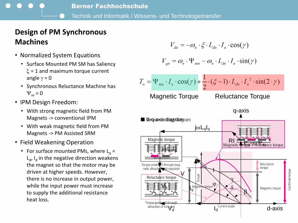
• Normalized System Equations

• Surface Mounted PM SM has Saliency = 1 and maximum torque current angle g = 0

• Synchronous Reluctance Machine has Ym = 0

• IPM Design Freedom:

• With strong magnetic field from PM Magnets -> conventional IPM

• With weak magnetic field from PM Magnets -> PM Assisted SRM

• Field Weakening Operation

• For surface mounted PMs, where Lq = Ld, Id in the negative direction weakens the magnet so that the motor may be driven at higher speeds. However, there is no increase in output power, while the input power must increase to supply the additional resistance heat loss.

Magnetic Torque Reluctance Torque

Technik und Informatik / Wissens- und Technologietransfer9

0 1 2 3 40

0.2

0.4

0.6

0.8

Torque vs. Speed (Normalized)

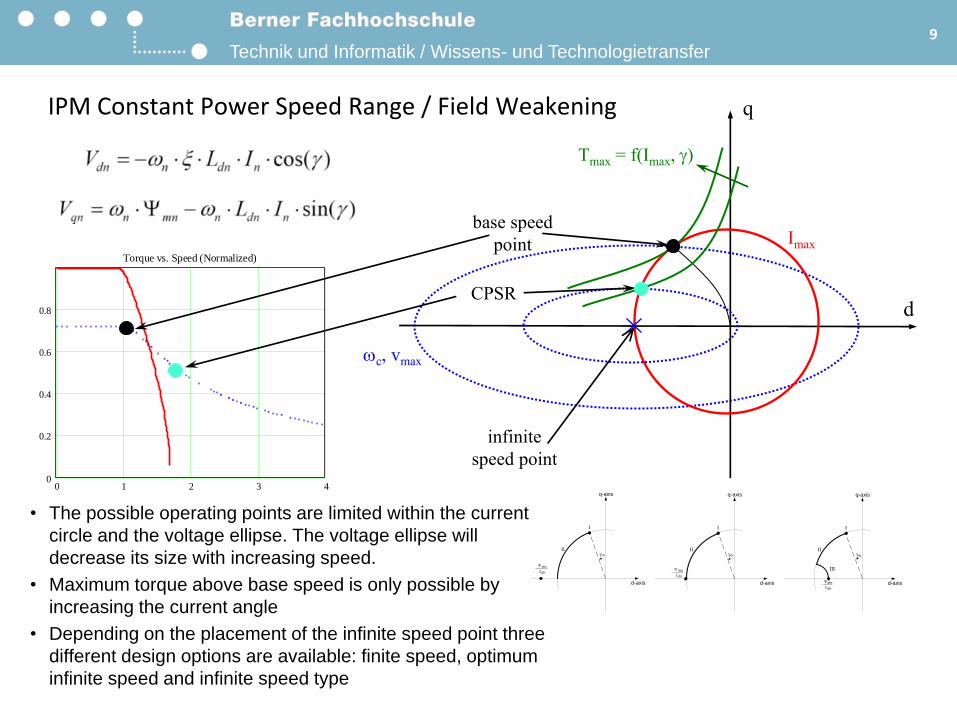
IPM Constant Power Speed Range / Field Weakening

• The possible operating points are limited within the current

circle and the voltage ellipse. The voltage ellipse will

decrease its size with increasing speed.

• Maximum torque above base speed is only possible by

increasing the current angle

• Depending on the placement of the infinite speed point three

different design options are available: finite speed, optimum

infinite speed and infinite speed type

d

wc, vmax

infinite

speed point

Imax

Tmax = f(Imax, g)

base speed

point

q

CPSR

II

q-axis

gm

mn

Ldn

Y

I

d-axis

d-axis

II

q-axis

gm

mn

Ldn

Y

I

d-axis

II

q-axis

gm

mn

Ldn

Y

I

III

Technik und Informatik / Wissens- und Technologietransfer10

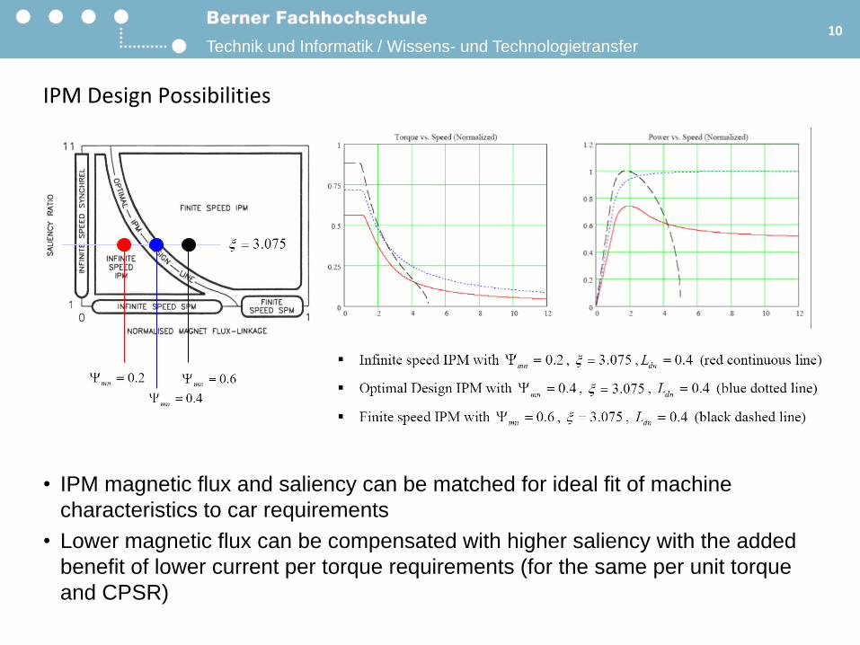
IPM Design Possibilities

• IPM magnetic flux and saliency can be matched for ideal fit of machine

characteristics to car requirements

• Lower magnetic flux can be compensated with higher saliency with the added

benefit of lower current per torque requirements (for the same per unit torque

and CPSR)


0 20 40 60 80 100 120 140

-1000

-500

0

500

1000

Speed[km/h]

Tor

que[

Nm

]

Energy [% of total] for 38 km Pendler Cycle

23kW - Cont Power

45kW - Peak Power

Torque for a=0 @ 0%

0

0.5

1

1.5

2

2.5

3

3.5

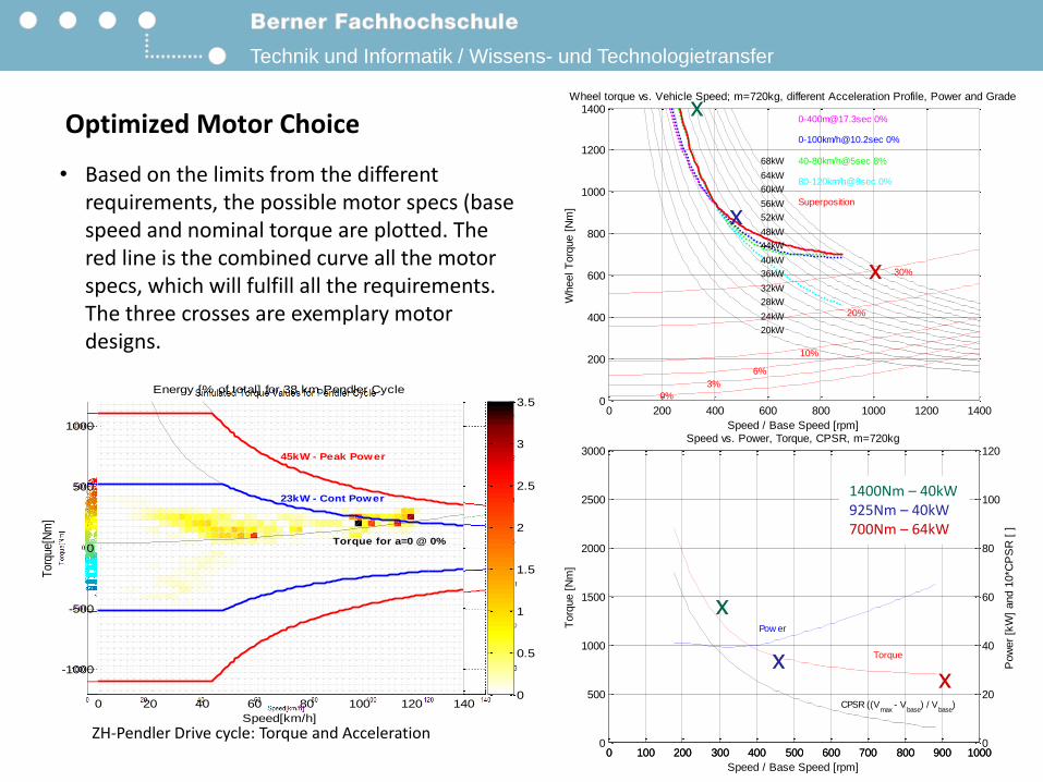
Optimized Motor Choice

• Based on the limits from the different requirements, the possible motor specs (base speed and nominal torque are plotted. The red line is the combined curve all the motor specs, which will fulfill all the requirements. The three crosses are exemplary motor designs.

ZH-Pendler Drive cycle: Torque and Acceleration0 100 200 300 400 500 600 700 800 900 1000

0

500

1000

1500

2000

2500

3000Speed vs. Power, Torque, CPSR, m=720kg

Speed / Base Speed [rpm]

Torq

ue [

Nm

]

Torque

0 100 200 300 400 500 600 700 800 900 10000

20

40

60

80

100

120

Pow

er

[kW

] and 1

0*C

PS

R [

]

Pow er

CPSR ((Vmax

- Vbase

) / Vbase

)

1400Nm – 40kW925Nm – 40kW700Nm – 64kW

xx

x

0 200 400 600 800 1000 1200 14000

200

400

600

800

1000

1200

1400

0-100km/[email protected] 0%

80-120km/h@8sec 0%

40-80km/h@5sec 8%

[email protected] 0%

Superposition

20kW

24kW

28kW

32kW

36kW

40kW

44kW

48kW

52kW

56kW

60kW

64kW

68kW

0%

3%

6%

10%

20%

30%

Speed / Base Speed [rpm]

Wheel T

orq

ue [

Nm

]

Wheel torque vs. Vehicle Speed; m=720kg, different Acceleration Profile, Power and Grade

x

x

x


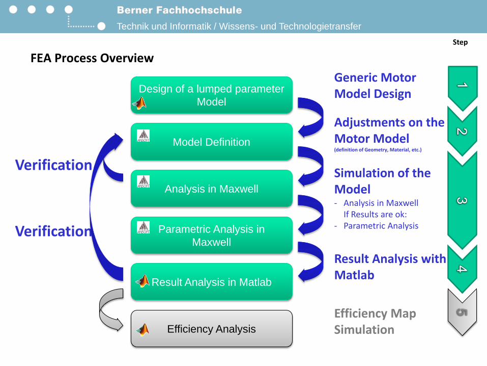
FEA Process Overview

Model Definition

Analysis in Maxwell

Parametric Analysis in

Maxwell

Verification

Adjustments on theMotor Model(definition of Geometry, Material, etc.)

Verification

Generic MotorModel Design

Step

Result Analysis in Matlab

Design of a lumped parameter

Model

Simulation of theModel- Analysis in Maxwell

If Results are ok:- Parametric Analysis

Result Analysis withMatlab

Efficiency Analysis

Efficiency MapSimulation

http://images.google.com/imgres?imgurl=http://people.seas.harvard.edu/~donhee/logo_ansoft.jpg&imgrefurl=http://people.seas.harvard.edu/~donhee/sponsors.htm&usg=__p4Nml36ptaqpvkNtYOblLoFB9E0=&h=177&w=180&sz=8&hl=en&start=22&um=1&tbnid=Ia5Z19iZrRQM9M:&tbnh=99&tbnw=101&prev=/images?q=maxwell+ansoft+logo&ndsp=18&hl=en&rls=com.microsoft:en-us:IE-SearchBox&sa=N&start=18&um=1




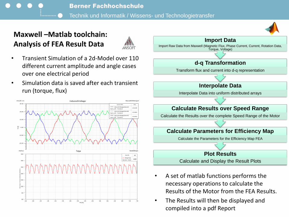
Maxwell –Matlab toolchain:Analysis of FEA Result Data

• A set of matlab functions performs the necessary operations to calculate the Results of the Motor from the FEA Results.

• The Results will then be displayed and compiled into a pdf Report

Plot Results

Calculate and Display the Result Plots

Calculate Parameters for Efficiency Map

Calculate the Parameters for the Efficiency Map FEA

Calculate Results over Speed Range

Calculate the Results over the complete Speed Range of the Motor

Interpolate Data

Interpolate Data into uniform distributed arrays

d-q Transformation

Transform flux and current into d-q representation

Import DataImport Raw Data from Maxwell (Magnetic Flux, Phase Current, Current, Rotation Data,

Torque, Voltage)

0.00 5.00 10.00 15.00 20.00 25.00 30.00

Time [ms]

-30.00

-20.00

-10.00

0.00

10.00

20.00

30.00

Y1

[V]

Ansoft LLC Maxwell2DDesign2InducedVoltage

Curve Info rms

InducedVoltage(phaseA)

back_emf : Transient14.5148

InducedVoltage(phaseB)


InducedVoltage(phaseC)


• Transient Simulation of a 2d-Model over 110 different current amplitude and angle cases over one electrical period

• Simulation data is saved after each transient run (torque, flux)

0.00 0.50 1.00 1.50 2.00 2.50 3.00 3.50 4.00 4.50 5.00 5.50 6.00 6.50 7.00 7.50Time [ms]

0.00

5.00

10.00

15.00

20.00

25.00

30.00

35.00

Mo

vin

g1

.To

rq

ue

[N

ew

ton

Me

ter]

Ansoft LLC Maxwell2DDesign2Torque

Curve Info avg

Moving1.Torque

load_losses : Transient24.0803



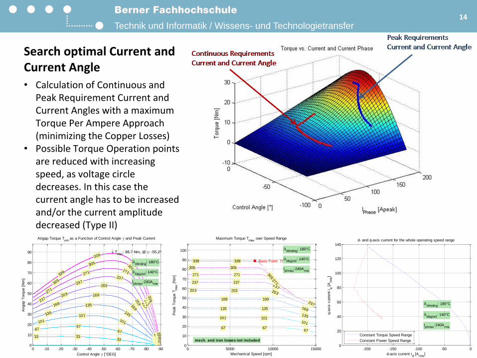
Search optimal Current andCurrent Angle

• Calculation of Continuous and Peak Requirement Current and Current Angles with a maximum Torque Per Ampere Approach (minimizing the Copper Losses)

• Possible Torque Operation points are reduced with increasing speed, as voltage circle decreases. In this case the current angle has to be increased and/or the current amplitude decreased (Type II)

14

33 3333

6767

67

67

101

101101

101

135

135

135

135

169

169

169

169

203

203

203

20

3

237

237

237

23

7

23

7

271

271271

27

1

27

1

305

305 305

30

5

30

5

339

339

339

33

9

33

9

Control Angle g [°DEG]

Airgap T

orq

ue [

Nm

]

Airgap Torque Tem

as a Function of Control Angle g and Peak Current

Winding

: 180°C

Magnet

: 140°C

Iphmax

:240Arms

Tmax

: 88.7 Nm, @ g: -55.2°

-90-80-70-60-50-40-30-20-1000

10

20

30

40

50

60

70

80

90

67 6767

101 101101

135 135

135

169 169

169

203 203 203

237 237237

237

271

271271 305

305305

339339 Base Point: 7900 rpm

Mechanical Speed [rpm]

Peak T

orq

ue T

max [

Nm

]

Maximum Torque Tmax

over Speed Range

mech. and iron losses not included

Winding

: 180°C

Magnet

: 140°C

Iphmax

:240Arms

0 5000 10000 150000

10

20

30

40

50

60

70

80

90

100

-200 -150 -100 -50 00

20

40

60

80

100

120

140

d-axis current id [A

rms]

q-a

xis

curr

ent

i q [

Arm

s]

d- and q-axis current for the whole operating speed range

Winding

: 180°C

Magnet

: 140°C

Iphmax

:240Arms

Constant Torque Speed Range

Constant Power Speed Range


Why not calculated Performance Curves from one single point of operation?

3333

67

67

101

101

101

135

135

135

169

169

169

203

203

203

237

237

237

271

271

271

305

305

305

339

339

339


q-a

xis

Inducta

nce L

q [

Henry

]

q-axis Inductance Lq as a Function of Control Angle g and Peak Current

Winding

: 180°C

Magnet

: 140°C

Iphmax

:240Arms

-80-70-60-50-40-30-20-100

100

200

300

400

500

600

700

800

900

3333

33

33

6767

67

67

101101

101

101

135

135

135

135

169

169

169

169

203 203

203

20

3

20

3

237 237

237

23

7

23

7

271 271

271

27

1

27

1

305 305

305

30

5

30

5

339 339

339

33

9

33

9


q-a

xis

Flu

x

q [

Vs]

q-axis Flux q as a Function of Control Angle g and Peak Current

Winding

: 180°C

Magnet

: 140°C

Iphmax

:240Arms

-90-80-70-60-50-40-30-20-1000

0.01

0.02

0.03

0.04

0.05

0.06

0.07

0.08

0.09

3333

33

67

67

67101

101

101

135

135

135

169

169

169

169

203

203

203

203

237

237

237

237

271

271

271

271

305

305

305

305

339

339

339

339


d-a

xis

Flu

x

d [

Vs]

d-axis Flux d as a Function of Control Angle g and Peak Current

Winding

: 180°C

Magnet

: 140°C

Iphmax

:240Arms

-90-80-70-60-50-40-30-20-100

-0.03

-0.02

-0.01

0

0.01

0.02

0.03

0.04

0.05

33

33 33

67

67 67

101

101 101

135

135 135

169

169 169

203

203 203

237

237 237

271

271271

305

305305

339

339

339


d-a

xis

Inducta

nce L

d [

Henry

]

d-axis Inductance Ld as a Function of Control Angle g and Peak Current

Winding

: 180°C

Magnet

: 140°C

Iphmax

:240Arms

-90-80-70-60-50-40-30-20-10

50

100

150

200

250

300

350

400

0 5000 10000 150000

50

100

150

200

250 No-Load Peak Phase to Phase Voltage @ 15000rpm: 434.3 V

Mechanical Speed [rpm]

Load a

nd N

o-L

oad P

hase V

oltage (

Peak V

alu

e)

Vph [

Vp]

Load and No-Load Phase Voltage over Speed Range

Winding

: 180°C

Magnet

: 140°C

Iphmax

:240Arms

b

jwLdId

jwLqIq

Eq=wYm

Iq

IV

IdVd

Vq

RI

b

gj

q-axis

d-axis

d

d-q-axis diagram

q

d

L

L

The effects of saturation on Ld and Lq are affecting the voltage equations and as a consequence the calculation of the dq-axis diagram


Efficiency Map

• Calculate Simulation Parameters forSimulation Points(Current, Current Angle, Rotation Speed, Simulation Time)

• Write Parameters as Variables intoMaxwellscript file for Simulation

• Simulation over at least two electricalperiods for each operation point in Maxwell

0 2000 4000 6000 8000 10000 12000 140000

5

10

15

20

25

30Points for efficency Parametric Analysis

Torq

ue [

Nm

]

Speed [rpm]

Maxiumum Requirements

Simulation Points

0.00 0.50 1.00 1.50 2.00 2.50 3.00 3.50 4.00 4.50 5.00 5.50 6.00 6.50 7.00 7.50Time [ms]

0.00

50.00

100.00

150.00

200.00

250.00

300.00

Co

reL

oss [W

]

Ansoft LLC Maxwell2DDesign2CoreLoss

Curve Info avg max

CoreLoss

load_losses : Transient210.6362 238.0068

0.00 0.50 1.00 1.50 2.00 2.50 3.00 3.50 4.00 4.50 5.00 5.50 6.00 6.50 7.00 7.50Time [ms]

-0.06

-0.04

-0.02

0.00

0.02

0.04

0.06

Y2

[W

b]

Ansoft LLC Maxwell2DDesign2FluxLinkage

Curve Info max

FluxLinkage(phaseB)


FluxLinkage(phaseC)


FluxLinkage(phaseA)



Core Loss Calculation

17

0.00

10.00

20.00

30.00

40.00

50.00

60.00

70.00

80.00

90.00

100.00

0.00 0.10 0.20 0.30 0.40 0.50 0.60 0.70 0.80 0.90 1.00 1.10 1.20 1.30 1.40 1.50

SPe

cifi

c C

ore

Lo

sse

s [W

/kg]

Induction Value [B]

Comparison of Maxwell Iron Loss Calculation with Measurement Data

Meas. 100Hz

Meas. 200Hz

Meas. 400Hz

Meas. 1000Hz

Meas. 2000Hz

Meas. 5000Hz

Meas. 10000Hz

100Hz

200Hz

400Hz

1000Hz

2000

5000

10000

Measured values as dots.Calculated lines are basedon Maxwell CoefficientsKh, Kc and Ke, which have beencalculated for each frequenceaccordingly.

0.00

10.00

20.00

30.00

40.00

50.00

60.00

70.00

80.00

90.00

100.00

0.00 0.10 0.20 0.30 0.40 0.50 0.60 0.70 0.80 0.90 1.00 1.10 1.20 1.30 1.40 1.50

SPe

cifi

c C

ore

Lo

sse

s [W

/kg]

Induction Value [B]

Comparison of Maxwell Iron Loss Calculation with Measurement Data

Meas. 100Hz

Meas. 200Hz

Meas. 400Hz

Meas. 1000Hz

Meas. 2000Hz

Meas. 5000Hz

Meas. 10000Hz

100Hz

200Hz

400Hz

1000Hz

2000Hz

5000Hz

10000Hz

Measured values as dots.Calculated lines are basedon Maxwell CoefficientsKh, Kc and Ke, which have beencalculated 100Hz data.

• Improvement of V12 by using multi-frequency data. Eliminates need to change data at each simulation step

• Maxwell uses dB/dt approach and not a fourier series Steinmetz based formula. This yields better results but requires at least two electrical periods of simulation data

Referenzpaper:D. Lin, P. Zhou, W. N. Fu, Z. Badics, and Z. J. Cendes: “A Dynamic Core Loss Model for Soft Ferromagnetic and Power Ferrite Materials in Transient Finite Element Analysis”


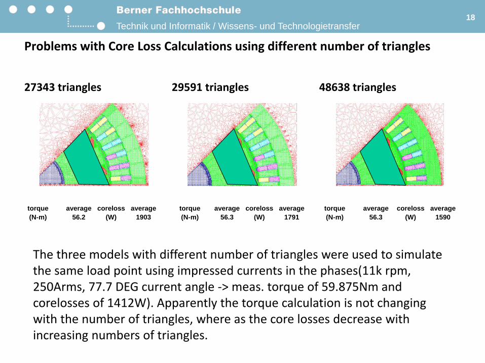
Problems with Core Loss Calculations using different number of triangles

27343 triangles

18

29591 triangles 48638 triangles

torque average coreloss average

(N-m) 56.2 (W) 1903


(N-m) 56.3 (W) 1791


(N-m) 56.3 (W) 1590

The three models with different number of triangles were used to simulate the same load point using impressed currents in the phases(11k rpm, 250Arms, 77.7 DEG current angle -> meas. torque of 59.875Nm and corelosses of 1412W). Apparently the torque calculation is not changing with the number of triangles, where as the core losses decrease with increasing numbers of triangles.


0.00 0.50 1.00 1.50 2.00 2.50 3.00 3.50 4.00 4.50 5.00 5.50 6.00 6.50 7.00 7.50Time [ms]

0.00

0.20

0.40

0.60

0.80

1.00

1.20

1.40

1.60

1.80

2.00

2.20

2.40

Co

reL

oss [kW

]


Curve Info avg max

CoreLoss

current_model_losses : Transient0.2628 2.4395

0.00 0.50 1.00 1.50 2.00 2.50 3.00 3.50 4.00 4.50 5.00 5.50 6.00 6.50 7.00 7.50Time [ms]

0.00

50.00

100.00

150.00

200.00

250.00

300.00

Co

reL

oss [W

]


Curve Info avg max

CoreLoss


Core Loss Calculation Methods• Impressed sinusoidal stator

currents

• Simplest Model, fast convergence

• Sinusoidal voltage supply and RL-parameter for winding

• long Convergence time

• Impressed PWM currents

• Taken from simulation data, good behavior, medium convergence (2 electrical periods), but needs high resolution

• Taken from measurement data for verification, needs treatment

• PWM voltage supply model

• Either in Maxwell or combined with Simplorer.

• Long simulation time, especially if mechanical model is used.

19

0.9 1 1.1 1.2 1.3 1.4 1.5 1.6

x 10-3

0

50

100

150

200

time [s]

pha

se

vo

ltag

e [

Vp]

phase voltage over electrical position

0 0.2 0.4 0.6 0.8 1 1.2 1.4 1.6 1.8 2

x 104

-600

-400

-200

0

200

400

600

Phase C

urr

ent

I p [

Ap]

Sampling Points []

P4 Phase Current measured at 5000rpm and 200Nm

0 0.2 0.4 0.6 0.8 1 1.2 1.4 1.6 1.8 2

x 104

-600

-400

-200

0

200

400

600

Phase C

urr

ent

I p [

Ap]

Sampling Points []

P4 Phase Current measured at 5000rpm and 200Nm

0 0.02 0.04 0.06 0.08 0.10

100

200

300

400

500

600

electrical position [°DEG electrical]

air

ga

p t

orq

ue

[N

m]

airgap torque over electrical position


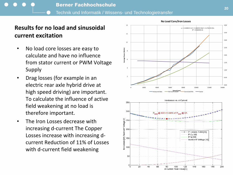
Results for no load and sinusoidal current excitation

20

y = -4.18381E-11x3 + 5.60691E-06x2 + 3.27622E-02xR² = 9.96694E-01

0.00

0.50

1.00

1.50

2.00

2.50

3.00

3.50

4.00

0

200

400

600

800

1000

1200

1400

0 2000 4000 6000 8000 10000 12000 14000

Ave

rage

Po

we

r (W

atts

)

Speed (rpm)

No Load Core/Iron Losses

measured data FEA Core Losses Corrected FEA Factor

• No load core losses are easy to calculate and have no influence from stator current or PWM Voltage Supply

• Drag losses (for example in an electric rear axle hybrid drive at high speed driving) are important. To calculate the influence of active field weakening at no load is therefore important.

• The Iron Losses decrease with increasing d-current The Copper Losses increase with increasing d-current Reduction of 11% of Losses with d-current field weakening


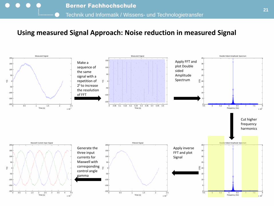
Using measured Signal Approach: Noise reduction in measured Signal

21

0 0.05 0.1 0.15 0.2 0.25 0.3 0.35 0.4 0.45 0.5

-150

-100

-50

0

50

100

150

Measured Signal:

Time [s]

Y(t

)

0 0.5 1 1.5 2 2.5

x 10-3

-200

-150

-100

-50

0

50

100

150

200Measured Signal:

Time [s]

Y(t

)

Make a sequence of the same signal with a repetition of 25 to increase the resolution of FFT

4.5 5 5.5 6 6.5 7 7.5 8

x 105

0

5

10

15

20

25

30

35

40Double-Sided Amplitude Spectrum

Frequency (Hz)

|Z(f

)|

Apply FFT and plot Double sided Amplitude Spectrum

0 0.5 1 1.5 2 2.5

x 10-3

-200

-150

-100

-50

0

50

100

150

200Filtered Signal

Time [s]

Y(t

)

4.5 5 5.5 6 6.5 7 7.5 8

x 105

0

5

10

15

20

25

30

35

40Double-Sided Amplitude Spectrum

Frequency (Hz)

|Z(f

)|

Apply inverse FFT and plot Signal

Cut higher frequency harmonics

Generate the three input currents for Maxwell with corresponding control angle gamma

0 0.5 1 1.5 2 2.5 3 3.5 4 4.5

x 10-3

-200

-150

-100

-50

0

50

100

150

200Maxwell Current Input Signal

Time [s]

Y(t

)


Core Loss calculation problems in Ansoft 2D

22

7.50 8.00 8.50 9.00 9.50 10.00 10.50 11.00 11.50 12.00 12.50 13.00 13.50 14.00 14.50 15.00Time [ms]

0.00

50.00

100.00

150.00

200.00

250.00

300.00

350.00

400.00

Co

reL

oss [W

]


Curve Info avg max

CoreLoss


0.00 0.50 1.00 1.50 2.00 2.50 3.00 3.50 4.00 4.50 5.00 5.50 6.00 6.50 7.00 7.50Time [ms]

0.00

2.00

4.00

6.00

8.00

10.00

12.00

14.00

16.00

Co

reL

oss [kW

]


Curve Info avg max

CoreLoss

current_model_losses : Transient0.8662 15.9693

0

100

200

300

400

500

600

700

800

900

0 0.5 1 1.5 2 2.5 3 3.5 4 4.5 5 5.5 6 6.5 7 7.5

Core

Loss

es [W

]

time [ms]

Core Losses: Proto II, 360V, 4‘000rpm, 60Nm

Average: 336.8352W

• Core loss computation is treated as "post process" in Maxwell 2D transient, that is, the core loss effects on the field are ignored.

• If the core loss effects on the field are taken into account, when there is a spike in an excitation, the core loss spike will reduce the field change, which in tune reduces the core loss spike.

• In Maxwell 3D transient, we can consider core loss effects on the field.

• Unfortunately, Maxwell 2D transient does not support this at present

• Results on the right:• Core Losses sinusoidal

Current: 298W• Core Loss PWM Current from

Simulation: 866W• Core Loss PWM Current from

Simulation, only Losses up to 8’00W taken into account: 337W


Conclusions

• Influence of PWM Supply on core losses is an important factor for the efficiency calculation of the motor as all of today's motor are based on PWM supply. In fully optimized systems efficiency gains in the motor due to higher PWM are optimized versus the higher switching losses in the Inverter.

• Iron Loss Calculation becomes an important task in the motor simulation process due to need for efficiency map calculation and optimization over the whole torque and speed range

• Computational Capabilities are still somehow limited and are based on manufacturer data with limited reliability due to old measurement setups. Manufacturer should modify test equipment to include higher frequencies and additional rotational losses

• Motor designers are used to 2D simulations to limit simulation time, fully transient simulation including taking into account the influence of eddy currents on the magnetic field should be therefore brought to Maxwell 2D as fast as possible

23


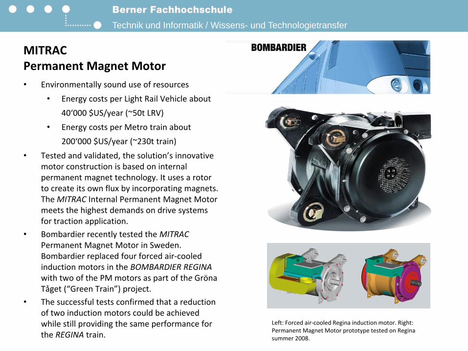
MITRACPermanent Magnet Motor

• Environmentally sound use of resources

• Energy costs per Light Rail Vehicle about

40‘000 $US/year (~50t LRV)

• Energy costs per Metro train about

200‘000 $US/year (~230t train)

• Tested and validated, the solution’s innovative motor construction is based on internal permanent magnet technology. It uses a rotor to create its own flux by incorporating magnets. The MITRAC Internal Permanent Magnet Motor meets the highest demands on drive systems for traction application.

• Bombardier recently tested the MITRACPermanent Magnet Motor in Sweden. Bombardier replaced four forced air-cooled induction motors in the BOMBARDIER REGINAwith two of the PM motors as part of the GrönaTåget (“Green Train”) project.

• The successful tests confirmed that a reduction of two induction motors could be achieved while still providing the same performance for the REGINA train.

Left: Forced air-cooled Regina induction motor. Right: Permanent Magnet Motor prototype tested on Regina summer 2008.


Research and Development Examples

25

New SAM: Cree AG, 2009, Switzerland/Poland

Equinox Fuel cell Car, General Motors, USA

ECUV, Sun Ya-Tsen University/HYB, China Angel Interceptor, domteknika AG, Switzerland


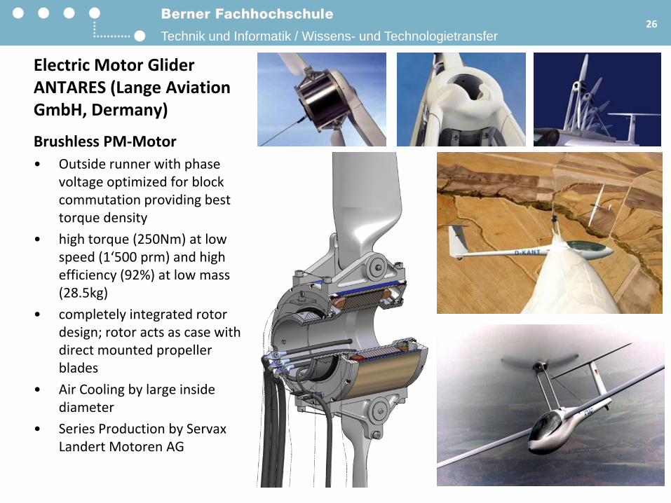
Electric Motor GliderANTARES (Lange AviationGmbH, Dermany)

Brushless PM-Motor

• Outside runner with phase voltage optimized for block commutation providing best torque density

• high torque (250Nm) at low speed (1‘500 prm) and high efficiency (92%) at low mass (28.5kg)

• completely integrated rotor design; rotor acts as case with direct mounted propeller blades

• Air Cooling by large inside diameter

• Series Production by ServaxLandert Motoren AG

26


Thank you very much for your attention

Dr. Andrea Vezzini

Laboratory for Industrial Electronics

Berne University of Applied Sciences

Tf.: +41 32 321 63 72

Fax: +41 32 321 65 72

email: [email protected]

Internet: www.ti.bfh.ch

27

Documents

IRON LOSS CALCULATION OF AN INTERNAL PERMANENT …...IRON LOSS CALCULATION OF AN INTERNAL PERMANENT MAGNET SYNCHRONOUS MACHINE FOR A FUEL CELL CAR Electric Drive System Research Activities