Embed Size (px)
Citation preview

1
IRAM NOEMAData Reduction CookBook
September 2010
Version 5.0
This document describes how to reduce NOEMA observations and gives some ideasto perform first analysis and imaging. Sect. 1 explains how to get started, from planningyour trip to Grenoble to having a project account. The standard procedure to calibrateNOEMA data with the clic software package is described in Sect. 2. A few instructionsto start the data analysis with the mapping software package are given in Sect. 3. Atheoretical description of the calibration as well as a description of the extended pipeline(or AoD) First Look report are annexed in Apps. A and B respectively.
DocumentationIn charge: A. Castro-Carrizo1, R. Neri1.Main past contributors: S. Guilloteau, R. Lucas, A. Dutrey, and S. Radford.
1. IRAM
Related information is available in:
• IRAM NOEMA: Introduction
• IRAM NOEMA: OBS Users Guide
• IRAM NOEMA: Atmospheric Calibration
• CLIC: Continuum and Line Interferometric Calibration
• MAPPING: Imaging and Deconvolution of Aperture Synthesis Data
• MIS: Millimeter Interferometry Simulation Tools
• GREG: Graphical Possibilities
• SIC: Command Line Interpretor

CONTENTS 2
Contents
1 Getting started 41.1 Preparing your travel . . . . . . . . . . . . . . . . . . . . . . . . . . . . . . 41.2 Working on the IRAM computers . . . . . . . . . . . . . . . . . . . . . . . 4
2 Data Calibration with CLIC 62.1 NOEMA pipeline and AoD notes . . . . . . . . . . . . . . . . . . . . . . . 62.2 How the data look like . . . . . . . . . . . . . . . . . . . . . . . . . . . . . 72.3 Getting started with CLIC . . . . . . . . . . . . . . . . . . . . . . . . . . 82.4 Open raw data file . . . . . . . . . . . . . . . . . . . . . . . . . . . . . . . 92.5 First Look . . . . . . . . . . . . . . . . . . . . . . . . . . . . . . . . . . . . 92.6 Standard Calibration . . . . . . . . . . . . . . . . . . . . . . . . . . . . . . 13
2.6.1 Select . . . . . . . . . . . . . . . . . . . . . . . . . . . . . . . . . . 142.6.2 Autoflag . . . . . . . . . . . . . . . . . . . . . . . . . . . . . . . . . 152.6.3 PhCor . . . . . . . . . . . . . . . . . . . . . . . . . . . . . . . . . . 152.6.4 RF calibration . . . . . . . . . . . . . . . . . . . . . . . . . . . . . 152.6.5 Phase calibration . . . . . . . . . . . . . . . . . . . . . . . . . . . . 172.6.6 Flux calibration . . . . . . . . . . . . . . . . . . . . . . . . . . . . 192.6.7 Amplitude calibration . . . . . . . . . . . . . . . . . . . . . . . . . 222.6.8 Print . . . . . . . . . . . . . . . . . . . . . . . . . . . . . . . . . . . 222.6.9 Usual difficulties . . . . . . . . . . . . . . . . . . . . . . . . . . . . 222.6.10 FAQ . . . . . . . . . . . . . . . . . . . . . . . . . . . . . . . . . . . 272.6.11 Other calibration procedures . . . . . . . . . . . . . . . . . . . . . 28
2.7 Data quality assessment . . . . . . . . . . . . . . . . . . . . . . . . . . . . 292.8 UV-Table Creation . . . . . . . . . . . . . . . . . . . . . . . . . . . . . . . 292.9 Calibrating and/or merging with data previous to 2007 . . . . . . . . . . 31
2.9.1 clic backwards compatible . . . . . . . . . . . . . . . . . . . . . . 312.9.2 uv-tables obtained before 04/2004 . . . . . . . . . . . . . . . . . . 312.9.3 Merging old and new data . . . . . . . . . . . . . . . . . . . . . . . 312.9.4 Continuum projects between 11/2005 and 01/2007 . . . . . . . . . 312.9.5 Very Old Projects . . . . . . . . . . . . . . . . . . . . . . . . . . . 33
3 First Instructions for Data Analysis with MAPPING 343.1 Operations on UV table . . . . . . . . . . . . . . . . . . . . . . . . . . . . 34
3.1.1 UVSHOW . . . . . . . . . . . . . . . . . . . . . . . . . . . . . . . . 353.1.2 UVSHIFT . . . . . . . . . . . . . . . . . . . . . . . . . . . . . . . . 363.1.3 UVFIT . . . . . . . . . . . . . . . . . . . . . . . . . . . . . . . . . 363.1.4 PLOTFIT . . . . . . . . . . . . . . . . . . . . . . . . . . . . . . . . 37
3.2 Imaging and deconvolution . . . . . . . . . . . . . . . . . . . . . . . . . . 383.2.1 SETUP . . . . . . . . . . . . . . . . . . . . . . . . . . . . . . . . . 38

CONTENTS 3
3.2.2 UVSHORT . . . . . . . . . . . . . . . . . . . . . . . . . . . . . . . 383.2.3 UVMAP . . . . . . . . . . . . . . . . . . . . . . . . . . . . . . . . . 393.2.4 SUPPORT . . . . . . . . . . . . . . . . . . . . . . . . . . . . . . . 403.2.5 CLEAN . . . . . . . . . . . . . . . . . . . . . . . . . . . . . . . . . 403.2.6 VIEW . . . . . . . . . . . . . . . . . . . . . . . . . . . . . . . . . . 42
A Appendix: Calibration Principles 43A.1 Standard Decomposition of Visibilities . . . . . . . . . . . . . . . . . . . . 43A.2 Baseline versus Antenna based calibration . . . . . . . . . . . . . . . . . . 46A.3 Plateau de Bure Online Calibration . . . . . . . . . . . . . . . . . . . . . . 46A.4 Offline Calibration; the rules of the game . . . . . . . . . . . . . . . . . . 47
B Appendix: Pipeline or AoD First Look 48

1 GETTING STARTED 4
1 Getting started
1.1 Preparing your travel
The day by day execution of Plateau de Bure projects can be followed athttp://www.iram.fr/IRAMFR/PDB/project.html. The status of the observations ofeach project can be checked at http://www.iram.fr/IRAMFR/PDB/ ongoing.html. Thescientific secretary informs the project principal investigator on the completion of his/herprogram and on the steps to follow to organize the travel to IRAM Grenoble, where thedata reduction is normally carried out. By following these instructions, you should get incontact with your local contact1 or with your collaborator at IRAM (who is the projectlocal contact) to find some convenient dates for both of you. Remote data reduction ispossible in exceptional cases, after agreement with the local contact and thereby withthe scientific coordinator.
For most projects a week at Grenoble is enough to finish the data calibration andperform first analysis. An experimented astronomer may need less time. We rec-ommend to spend one day on data analysis after calibration, so that we can help ifthere are difficulties and return back to data calibration if needed. You are invitedto consult with your local contact before deciding on the duration of your stay. Toavoid overbooking the computer facilities, no more than two groups are accepted si-multaneously. You should consult the visitor list before discussing dates with the localcontact. You will tell the scientific secretary on the agreed dates as soon as possi-ble, so that she can book a computer, and may help in hotel booking and in otherquestions related to your visit. Visits must be announced at least two weeks in ad-vance. You can consult the conditions for financial support for visiting astronomersat http://www.iram.fr/IRAMFR/PDB/bure mission.html. Finally, note that IRAM isclosed from Friday 6pm to Monday 8am.
1.2 Working on the IRAM computers
As soon as you arrive at IRAM Grenoble, an account is created for your project. Projectaccounts are in general allocated for a period of two weeks and are automatically removedat the end of that period (with no archiving or warning). You should get in contact withyour local contact in case you need more time.
At your arrival a computer at the IRAM terminal room is booked for the reductionof your project. Your local contact will provide some information on the computerdirectories, download the raw data and have a first look with you at the calibrationprocedure.
1A local contact is assigned to each A and B-rated project which does not have in-house collaborator.He/She assists you in the preparation of observing procedures and in the data reduction.

1 GETTING STARTED 5
Project accounts contain a README file, the reports, calib and maps directoriesand the tmp −> /scratch/xxxx/ link. In README you will find a description ofthe account directories and some other helpful information. The reports directorycontains the calibration results obtained by the pipeline2, sometimes also those from animproved calibration by the astronomer on duty (AoD)3, and AoD’s notes to help withthe calibration (Sect. 2.1). The data calibration is, by default, performed in the calibdirectory, further data analysis in maps.
In order to download the project raw data, the command getproj must be executedin the shell prompt. The data are stored in the scratch directory linked by tmp, and arevisible from all clic sessions launched on the computer where getproj was executed.
By default the gildas daily version is used. You can execute ”gagiram mmmyy”(mmm = month, yy = year) to switch to a previous gildas release.
At the end of the calibration you may want to save a copy of the project account.Reduced data can either be transferred via scp to your home institute or archived onDVDs. From the account home the command “buildDVD .” allows you to burn in aDVD all the things there contained. Note that the IPB data files are in the scratch ofthe assigned computer and so by keeping the default distribution they are not saved inthe DVD. Finally, it is strongly recommended to check the integrity of the recorded databefore the account expires.
2Pipeline normally refers to the automatic calibration taking place at Bure, which is afterwardsverified, sometimes also improved, by the astronomer on duty.
3Astronomer on Duty taking care of the NOEMA observations and of the first data calibration

2 DATA CALIBRATION WITH CLIC 6
2 Data Calibration with CLIC
clic is the software to calibrate NOEMA data. The calibration of most projects iscarried out with a few interactive procedures and widgets provided within clic, so mostastronomers do not need to know much about clic commands. We recommend howeverto have a look in the clic manual4 at the following commands: help, file, find, list,plot, set x and set y. During the calibration you will become familiar with others, e.g.solve. In general we recommend to read the clic manual to have a deeper understandingof the calibration possibilities.
In some of the following sections, paragraphs written with italic fonts are aimed tosolve problems that may appear in the calibration. You can skip these paragraphs in afirst reading.
2.1 NOEMA pipeline and AoD notes
In the project account, the reports directory contains the first calibration results pro-duced or revised by the AoD (Sect. 1.2). The gzipped postscript and ascii files reporton the calibration. Particularly those whose names include -pipe result from the auto-matic data reduction or pipeline (Sect. 1.2). You will get familiar with the calibrationreports in Sects. 2.4, 2.5 and 2.6. The AoD performing the observations evaluates thedata quality and calibration, and may write notes in the ascii file of extension note. Itis recommended to read the notes relative to each track before starting its calibration.The files of extension hpb, so-called header files, store the parameters derived from thecalibration.
Having a look at the automatic reports before starting the calibration may be useful,mainly for an experimented astronomer. They can be used, for instance, to decide onthe first track to calibrate, likely the one with the best flux calibration. In addition, notethat the AoD at Bure performs a comprehensive analysis of the observations, and his/hernotes (in the note file) may be useful to identify problems, which perhaps are visible insome of the plots of the First Look report (see Sect. 2.5 and App. B). Recommendationsconcerning the calibration might also be added to the AoD notes.
Nowadays the pipeline is distributed with every release of GILDAS, although itcan only be used with data obtained later than January 2007. You just need to type“@pipeline ‘project name’ ‘date’ ” and the pipeline will be launched, producingoutputs very similar to those obtained at the observatory. It has become usual amongNOEMA users to start the data calibration by launching the pipeline. If this first cali-bration is not satisfactory, the analysis of the pipeline report, with the help of the AoDnotes and the local contact, allow improving easily the data calibration. Anyway, werecommend to have a critical look at the pipeline output protocols before making useof the hpb files. Particularly, it is known that the Data Quality Assessment procedure
4available on-line at http://www.iram.fr/ IRAMFR/GILDAS/

2 DATA CALIBRATION WITH CLIC 7
launched at the end of the calibration often flags out more data than actually needed. Ifyou plan to recalibrate all or parts of the calibration from the pipeline-produced hpbfile, we recommend first to remove all the Data Quality Assessment flags by using thefollowing commands:
file both ‘file name.hpb’findstore flag redu /ant all /resetstore flag redu /base all /reset
At the end of the new calibration you can use the Data Quality Assessment pro-cedure (Sect. 2.7) to flag the undesirable data according to the needs of your project.
2.2 How the data look like
Let us assume that we are already looking at the data, in clic. After typing in clicfind and later list we will see, e.g.:
60 7684 QA12 3C454.3 P CORR CO10 6Cq-N17 12-NOV-2007 21:58 2.961 7685 QA12 3C454.3 P CORR CO10 6Cq-N17 12-NOV-2007 21:59 2.962 7686 QA12 3C454.3 P CORR CO10 6Cq-N17 12-NOV-2007 22:00 2.9
where each line corresponds to an observation subscan5. Each subscan contains thefollowing information:
- First column: Observation number- Second column: Scan number- Third column: Project name- Fourth column: Source name- Fifth column: Type of source (O=object, P=phase calibrator)- Sixth column: Type of scan procedure- Seventh column: Line name- Eighth column: Array configuration, i.e. antenna positions- Nineth column: Date- Tenth column: UT time- Eleventh column: Hour angle
The usual observational procedures (column sixth) and characteristics are:
CORR: cross-correlation; 1 subscan (ss) is obtained per scanGAIN: cross-correlation to measure the sideband rejection; 1 ssFOCU: focus measurements in all the antennas; 5 ssPOIN: interferometric pointing in all the antennas; 2 ss
5A subscan (which is a scan partition) is the shortest acquisition for which spectral information isstored. Frequency-averaged acquisitions are stored for each second, and are known as records

2 DATA CALIBRATION WITH CLIC 8
FLUX: cross-correlation to measure the flux; 1 ssIFPB: IF passband calibration, by observing a noise diode; 2 ssAUTO: autocorrelation; 1 ssCALI: atmospheric calibration, autocorr. on SKY, HOT [COLD] load; 2 [3] ssSKYD: sequence of autocorrelations to calibrate the 22 GHz receivers; 12 ss
By using the mentioned procedures, a typical sequence of observations is:
- Receiver tuning followed by a sideband gain measurement- Radio frequency passband calibration on a bright source- Acquisitions on at least a flux calibrator, MWC 349 if possible- Check the pointing and focus on the predefined phase calibrator(s)- Possibly a flux measurement on this calibrator(s)- Cross-correlations on the phase calibrator(s)- Cross-correlations on source
About 3 minutes are spent on each phase calibrator, some more time if pointing andfocus are performed, every ∼ 23 minutes on source. Pointing and focus are normallyrepeated every two transitions of ∼ 23 minutes on source. IFPB, AUTO and CALI scansare obtained before correlations to calibrate the observations in real time (see Sect. A.3).
2.3 Getting started with CLIC
Just type clic in the shell prompt, and click on the clic widget shown in Figure 1 tohave the menu.
Figure 1: clic menu
In the following sections we describe the steps to follow in order to calibrate a standardproject, following the options listed from top to bottom in the clic menu.

2 DATA CALIBRATION WITH CLIC 9
2.4 Open raw data file
The data obtained at Plateau de Bure are stored in files of extension IPB. The parametersderived from the calibration are stored in files of extension hpb (or header files). A nakedversion of these files can be created with the option Open raw data file (Figure 2) inthe clic menu (Figure 1).
First of all, the location of the raw data (IPB files) must be defined, either by clickingin RAW DATA DIRECTORIES (see Figure 2) or within the .gag.dico gildas file. In theIRAM project accounts (see Sect. 1.2) the location of the raw data is already predefined.A raw data file must be selected among the Project Date choices. OPEN and FINDopens this file and proposes a standard name for the output file. CREATE HEADER FILEcreates a hpb file ready to calibrate the data in antenna-based mode. By default Mode(in the widget) is NEW, and so a new hpb file is created each time. By selecting OLD,visibilities can be added to an existing hpb file, which is very convenient if observationswere contiguous in time.
Figure 2: Open raw data file, in the clic menu.
In this and the following widgets there are at the top the options GO and ABORT. GOis aimed to run all the options proposed as clickable buttons, from left to right, with nostop. In general, its use is only recommended for the First Look (see Sect. 2.5). ABORTcloses the widget and returns to the parent widget.
As mentioned in Sect. 2.1, the hpb files resulting from the NOEMA pipeline calibra-tion are given in the directory reports. We recommend not to use them to create thefinal uv-tables since, for the time being, they were not created with this purpose and somay include severe flags or artifacts due to a further AoD analysis.
2.5 First Look
To have a look at the conditions in which the observations were obtained click on theFirst Look in the clic menu (Figure 1). An extended version of the First Look is

2 DATA CALIBRATION WITH CLIC 10
used by the AoD and by the pipeline procedure (see App. B).An hpb file name is needed to start with the First Look widget (see Figure 3). The
scan range can also be specified. By default all the scans are taken into account (i.e.from 0 to 10000). The receiver with which the source(s) was observed is determined byclicking on Select.
Select is also necessary to assess the presence of data, and to define variables neededin the following calibration steps. The options from Meteo to Water can be clicked withno defined order. Each of them creates one or two plots and then pauses waiting for a“continue”, in the clic prompt, in order to save the displayed plots in postscript files.Print combines all these postscript files in a file called show-’date’-’projectname’.ps,including also a description of the observational setup and a detailed scan list.
This package is actually not interactive since it does not admit an input other than“continue”. With GO we can therefore obtain the same result as by clicking through thebuttons, from Select to Print. It is recommended to check the First Look report toidentify instrumental features, errors, verify weather conditions, etc. This informationbecomes particularly relevant to take adequate decisions in case of calibration difficulties.
Note that all the plots created with the First Look are presented for physical an-tennas6, while the calibration procedures refer to logical antennas7. Sometimes the AoDrefers in his/her notes to physical antennas, but note that all the clic commands referto the logical ones. In the section 1.2 of the calibration report (see Sect. 2.1 and 2.6),efficiencies are presented for logical antennas, the equivalent physical numbers are showninto parenthesis.
Select, in addition to selecting the used receiver(s), adopts default settings for datapresentation, reports on the amount of correlations obtained, defines scan ranges betweentunings by looking at the gain scans, reports on the used baselines and antennas, onthe array configuration, on the used calibrators and their fluxes, and the tuned band.Select also introduces in the widget the option to select telescope configuration if thatchanged during the observations. Information is given in the line of commands, which isspecially relevant for calibration (as shown in Figure 4).
Meteo provides information on the atmospheric conditions at the time of the obser-vations: Ambient temperature (in K), relative humidity (%), pressure (mbar) and themean and maximum wind speed (m/s).
6Each NOEMA antenna has a reference number that identifies it, from 1 to 6 corresponding to theorder in which they were built. When we refer to the antennas by using this reference number, we callthem physical antennas.
7clic uses a numbering for the antennas proper to each observation, going from 1 to the number ofused antennas. We refer to logical antennas when we use their reference number in clic. Note thatthe logical antennas differ from the physical ones if the array has less than 6 antennas and the missingantennas are not the last ones.

2 DATA CALIBRATION WITH CLIC 11
Figure 3: First Look, in the clic menu
Elev-Azi plots the elevation and azimuth of each scan, so that we can see the relativeposition of a source with respect to the calibrators.
Poin-Foc presents the pointing corrections (in arc seconds) in azimuth and elevation, andthe focus corrections (in mm) per antenna. Note that pointing and focus measurementsare performed typically every ∼ 50 min (i.e. every two transitions on source)
Tracking shows the rms of the tracking variations (in arc seconds) in azimuth andelevation.
Tot. Pow. displays the total power (in K) obtained per correlator input8.
Tsys plots the system temperature (in K) along the track, for the tuned and the rejectedband. Note that after January 2007 all receivers installed at Plateau de Bure are operatedin single side-band mode. A plot is created per correlator input8.
Water shows the values derived for the water vapor pressure (in mm) by modeling theatmospheric behavior from the data obtained with the astronomical receivers. The watervapor pressure (WVR H2O) obtained from the 22GHz receivers is also shown. Note that the
8There are two correlators at the observatory: 1) The Narrow-band correlator accepts two 1 GHz inputsignals, from the 4 GHz band obtained per polarization. Narrow inputs refer to the two 1GHz-bandwidthsignals entering into the narrow-band correlator, which correspond to quarters of the receiver bands. Theastronomer decides on the configuration of the eight spectral units of the narrow-band correlator withinthe two selected Narrow inputs. 2) The Widex correlator is composed of four units, each one accepting2 GHz bandwidth. Units 1 and 3 and units 2 and 4 are placed consecutively to cover a bandwidth of3.8 GHz respectively in the IF of H and V polarization receivers. Widex inputs correspond hence to thefour Widex units)

2 DATA CALIBRATION WITH CLIC 12
Figure 4: Information given in the line of commands after Select, in the First Lookand the Standard Calibration sections.

2 DATA CALIBRATION WITH CLIC 13
Figure 5: Standard Calibration, in the clic menu
22GHz receivers are only sensitive to water vapor, while the astronomical ones permit toobtain a rough estimate of the water in the atmosphere, including liquid water. A plotis created per correlator input8.
Print combines all the plots in a file of name show-‘date’-‘projectname’.ps.
AoD or pipeline First Look: The astronomer on duty carrying out the observationsperforms a deeper analysis of the data. The file created by the AoD First Look includesmore technical plots, related to receiver calibration, bandpass stability, correlator tweaks,22 GHz receivers, cables transporting the synthesizer signals, etc (briefly described inApp. B). The AoD may include remarks in the project note file (see Sect. 2.1) if theinspection of these plots reveals problems to be considered in the calibration.
2.6 Standard Calibration
This tool is designed to calibrate a standard NOEMA project. The name of the hpb(header) file must be specified in the Standard Calibration widget (Fig. 5) to start. Alimited scan range can be selected to perform a complete or partial calibration. By defaultall the scans are considered. The receiver band used in the observations is determinedby clicking on Select.
The calibration must be done by clicking on the proposed steps from left to right.Select is so needed at first, and also before repeating any part of the calibration. Thelast option Print combines all the postscript files created of each calibration step in asingle file called ‘date’-‘projectname’.ps. This package is an interactive tool which pauses

2 DATA CALIBRATION WITH CLIC 14
for an input from the astronomer. It is not recommended therefore to click on the GO(see Sect. 2.4).
The option Use previous settings (in the widget; Fig. 5) permits to adopt set-tings coming from a previous calibration of the selected hpb file, with respect to theatmospheric phase correction, scan ranges, selected bandpass calibrator, etc.
Finally, note that all the plots created within the Standard Calibration are pre-sented for logical antennas, which are sometimes different from the physical ones shownin the First Look outputs (see Sect. 2.5 and App. B).
2.6.1 Select
It selects the used receiver band(s), establishes defaults for data presentation, reports onthe amount of correlations obtained, scan ranges between tunings, array configuration(s),lists the physical baselines and antennas, builds a first flux list and reports on the tunedband. In addition, it defines internal variables which are later used by the calibrationprocedures.
The procedure also selects the RF calibrator, at first the brightest observed source,otherwise that selected in a previous RF calibration. The selection is reported in theline of commands, as shown in Figure 4. Sometimes, because of technical problemsor to improve sensitivity, another calibrator must be considered. In those cases “letband source ‘a new calibrator’ ” must be typed in clic to select ‘a new calibrator’.
Select deduces which are the phase calibrators observed alternatively with thesource, hence suitable to calibrate phase and amplitude evolution in time. The names ofthe selected calibrators are stored in the variable phcal. You can decide about the con-tent of phcal as follows: “let phcal ‘calibrator1’ ‘calibrator2’ ... ”. Note that “let phcal‘*’ ” should be selected if the (frequency averaged) phases from the H and V polarizationreceivers are not identical, which for instance can be seen in the RF phases plot in theFirst Look (see more details in Sect. 2.6.5).
By default, the atmospheric phase corrections derived from the 22GHz receivers areused according to the PhCor evaluation (see Sect. 2.6.3). However, sometimes it is rec-ommended (by the Autoflag procedure or by the AoD) not to use the phase corrections,for instance due to problems with the 22GHz receivers. “let do atm no” allows ignoringthe atmospheric phase corrections.
Several gain ranges: From time to time, the Select procedure pauses to informon the presence of different gain ranges, i.e. scan intervals with different tuning charac-teristics. The RF calibration is then performed independently for each gain range (i),and a calibrator is so assigned to the variable “band source[i]” for each range. When theprocedure pauses, continue should be typed in the line of commands to continue.

2 DATA CALIBRATION WITH CLIC 15
2.6.2 Autoflag
Different verifications are performed in all the obtained scans, which are flagged if anoma-lies are identified. For instance, Autoflag checks that the timing of the acquisitions iscorrect. It also verifies that no source data are surrounded only by flagged calibratoracquisitions, which for instance may happen if an antenna is shadowed. A message isgiven for information if problems are found, reporting about introduced flags.
Warnings, periods of observational peculiarities: If the observations were ob-tained in periods with special conditions or difficulties, a message is shown to informabout it and about the possible consequences in the calibration.
2.6.3 PhCor
PhCor compares the amplitude of each scan with and without atmospheric phase cor-rection. The phase correction is only adopted when it reduces the phase decorrelationwithin each scan. Note that the spectral units, L01 to L12, do not store informationon time scales smaller than a scan, while the continuum units, C01 to C12, do so; twostreams of data are so stored at Bure for each L0i and C0i unit, respectively with andwithout atmospheric phase correction.
A green line on the bottom of the plot produced during the flux calibration (see Figure9) shows, when being above zero, the scans for which the program PhCor activates theatmospheric phase correction.
In addition, this procedure checks for interferences in the WVR channels, if it wasnot done before (for instance by the pipeline).
Note that the data are not corrected for atmospheric decorrelation if “let do atm no”was selected (see Sect. 2.6.1).
At the end, a procedure is launched to verify if the phase calibrators are polarized,setting the variable do avpol accordingly (see Sect. 2.6.7) to define the amplitude cali-bration mode.
2.6.4 RF calibration
The goal is to measure the receiver bandpass (RF) to calibrate the source data. Forthis, a bright calibrator is observed for some minutes. By default, in a first calibrationthe procedure Select selects the brightest observed source for the RF calibration. Theselected RF calibrator can be changed by modifying the variable “band source” as ex-plained in Sect. 2.6.1. If several gain ranges are found, an independent RF calibration isperformed for each range.
The procedure pauses to propose fits for amplitudes and phases for each correlatorinput (as shown in Figure 6); by default the solutions for the Narrow correlator inputsare obtained with “solve rf 12 20 /plot”, where “12” is the polynomial degree to fitamplitudes and “20” for phases (higher degrees are used for the Widex correlator units).

2 DATA CALIBRATION WITH CLIC 16
Figure 6: Example of the RF calibration of data obtained for the second Narrow corre-lator input
Changing the polynomial degrees with respect to the ones proposed by the automaticprocedure rarely improves the RF calibration. In the pause, “continue” (or “c”) shouldbe typed to accept the solution and store the calibration parameters in the hpb file.
Sometimes the fit of the bandpass looks poor with deviations of a few degrees (in phase) or afew percents (in amplitude) between the measured data and fits are observed. For the time beingthere are no simple means to reduce these small differences. In general, they have no influenceon the results.
Sometimes the procedure crashes (when fitting) because the data of an antenna is flagged.Two solutions exist: (1) Mask (see point 2 in Sect. 2.6.10) shadow, saturati[on] or redu[ction]flags to use these data for the RF calibration if the signal to noise ratio is good enough. (2) Selectanother calibrator by typing “let band source ‘a new calibrator’ ” as indicated in Sect. 2.6.1.
If delays are observed (constant slope in phases vs. frequency for one or more antennas) wemay correct for it to decrease the phase decorrelation within scans. By using the commands “solvedelay /plot” and “modify delay” we can correct for this (see Sect. 2.6.9).
Differences in the LO1ref frequencies result in frequency offsets in the RF amplitude profiles.

2 DATA CALIBRATION WITH CLIC 17
If the AoD (through the project notes) informs you on the presence of a big LO1ref jump (whichis often linked to cable phase jumps) we recommend to calibrate the RF with the strongest phasecalibrator observed cyclically with the source, for which the source LO1ref frequency was properlyconsidered.
2.6.5 Phase calibration
In most projects we observe, alternatively to the source(s), one or two phase calibrators,for which ‘ideal’ phases (without instrumental contribution) are known to be zero forall the baselines. The track of these phases allows us to measure and remove possibleinstrumental contributions. The phase fittings for the calibrators observed cyclicallywith the source (set by Select, Sect. 2.6.1) are obtained with the command “solve phase/plot”. Breaks and jumps can be introduced in the fit with the option “solve phase /break‘break degree’ ‘break time’ ”. Break degree is the order of the polynomial derivative thatis discontinuous at the break point, the sharpest one being 0. Break time is the UT time(h) at which the break should happen. (See two examples of phase calibration in Figure7.) The option “/weight” can be used to take into account the weight (∼ SNR) of thedifferent calibrators, and “/polynomial” to impose polynomials of a given degree (thelast option is incompatible with the use of breaks). More information can be found inthe clic manual, or by typing “help solve phase” in clic. The procedure pauses afterproposing a fit. A previous solution can be removed from the plot with “clear seg” to trya new one. A solution is accepted by entering “c” in the line of commands. The phasesare calibrated independently for each polarization, and stored in the hpb file at the endof the procedure.
The choice of phase calibrators used to calibrate the source phases and amplitudes isperformed by Select (see Sect. 2.6.1). If you disagree with the choice, it can be modi-fied with “let phcal ‘list of calibrators’ ”. The phases and amplitudes of the calibratorsnot included in this ‘list of calibrators’ are self-calibrated. Note that if the frequency-averaged phases from H and V polarization receivers are not equal (which for instancecan be seen in the RF phases plot, see Sect. B) self-calibration should be avoided, andhence “let phcal ‘*’ ” should be entered after Select (Sect. 2.6.1).
If due to some poor data obtained in a limited time interval, the fit fails in other intervalin which the phases seem well constrained, we can divide the phase calibration in two parts, byspecifying the scan intervals in the main calibration widget. We should just pay attention that nosource data remains uncalibrated between the two selected intervals.
From time to time the procedure crashes because too many calibrator data are flagged for anantenna or baseline. To find a proper solution for the other baselines we can just mask (see point2 in Sect. 2.6.10) whichever the flags, solve the phases for all baselines, and reset at the end thesemasks. Verify at the end that the source data that were calibrated with flagged calibrator data arenot used.
If the data obtained for a calibrator are too bad, and are not needed in the calibration, we canflag them as indicated in Sect. 2.6.10.
2 DATA CALIBRATION WITH CLIC 18
Figure 7: Example of the phase calibration of data obtained for the horizontal polariza-tion. The command “solve phase /plot” was used in the first plot, “solve phase /plot/break 1 14.7 3 15.2” was used in the second one. The introduction of sharp breaks inthe phase calibration should always result from an analysis of the reasons for such phasejumps.

2 DATA CALIBRATION WITH CLIC 19
2.6.6 Flux calibration
When clicking on FLUX (in the CLIC menu; Fig. 1) a widget similar to the one shownin Fig. 8 is opened. The flux calibration is an iterative process in which the known fluxof one or more calibrators is fixed to determine the efficiencies (Jy/K) of the antennas,which are then used to estimate the flux of the other calibrators. When a flux is fixed,SOLVE derives efficiencies and fluxes. GET RESULT, STORE, and PLOT store the solved fluxdensities and plot the amplitudes scaled by the derived fluxes (in K/Jy). These scaledamplitudes correspond to the inverse of the antenna efficiencies, that, in an ideal project,should remain constant and equal to their nominal values.
The amplitudes obtained for a calibrator often vary along the track due to effects ofa changing atmosphere or instrumental problems. Antenna efficiencies should be esti-mated by considering the best data ranges. Observational glitches, data obtained withbad pointings or focus measurements, or limited intervals of bad data should not beconsidered. If for an observed polarization amplitude oscillations on a 24 hour scale areobserved, this is often an indication of that the emission is polarized. Having H and Vpolarizations is needed to confirm the presence of polarized emission. (The degree of po-larization of the NOEMA phase calibrators is evaluated and archived at the observatory,and so can be checked by your local contact if needed.) Anyway, there is nothing to doin the flux calibration with respect to this. The Scan List option permits to select thescan ranges to be considered in the calculation of fluxes and efficiencies. After PLOT, scannumbers can be determined by using the command “cursor” and clicking on the display(an example is shown in Figure 9).
All the calibrators observed during the track are shown in this widget. Currentlythe main flux calibrator is MWC 349, which is observed in most of the projects; whenincluded, a flux is proposed to be fixed, as we can see in Fig. 8. Its use must be how-ever considered by checking the quality of the observed correlations: i.e. correlations onMWC 349 showing a big scatter in amplitude should not be considered unless they arerepresentative of the track observing conditions. The other calibrators, the one used tocalibrate the RF and also the phase calibrators, can be used in this process. Their fluxmay be known from other tracks observed close in time. Note also that we monitor theflux of the brightest calibrators. Your local contact can provide you this information,and also an estimate of the right efficiencies with a reasonable accuracy. For example, fora track observed in good conditions the expected efficiencies for the different antennasshould range from 20 to 25 Jy/K, from 25 to 32 Jy/K, and from 32 to 45 Jy/K forreceiver bands 1, 2, and 3 respectively. Values much larger than those expected shouldbe well explained by the observational conditions. Efficiencies significantly smaller arenot possible.
By properly using this method, the absolute calibration obtained is typically preciseto less than 10% at 3mm and ∼ 20% at 1mm. Special attention should be payed to therelative flux calibration between different tracks; normally the different tracks provide

2 DATA CALIBRATION WITH CLIC 20
Figure 8: Flux Calibration widget, showing on top the solved antenna efficiencies. Notethat these are characteristics of the antennas, and the different values obtained betweenantennas should be well understood by the AoD at the time of the observations andlikely also by your local contact. For instance, the low efficiency of A6 at the moment ofthese observations was due to a polluted injected LO signal; a new LO box was installedin A6 just after these observations. In the second row we define the scan intervals to beconsidered in the flux calibration.
2 DATA CALIBRATION WITH CLIC 21
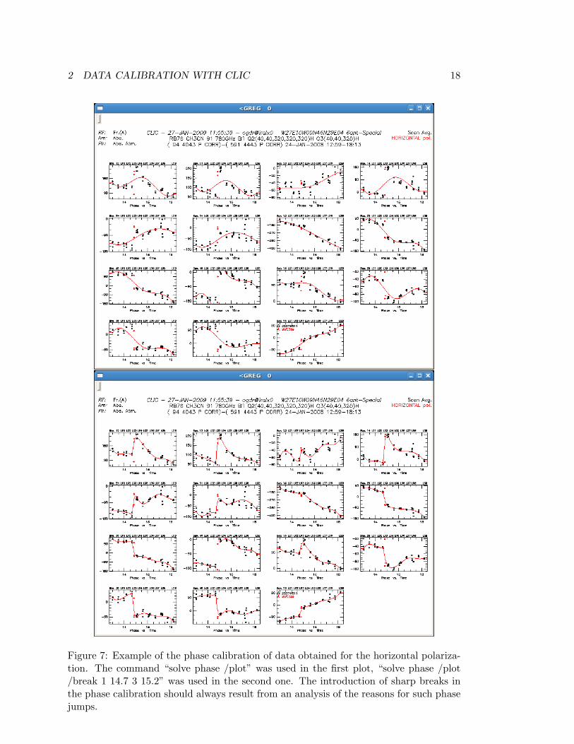
Figure 9: Flux Calibration plot, showing the amplitudes scaled by the solved fluxes.Note that the amplitudes from both Narrow correlator inputs are averaged in this plot.
complementary information in the uv-plane, and so a wrong relative flux calibration canbe interpreted as source structure.
As mentioned in Sect. 2.6.3 the green lines at the bottom of the plots show, whenbeing above zero, the regions in which the atmospheric phase correction is applied asresulted from PhCor.
Note finally that the option CHECK, at the top of the FLUX calibration widget (Fig.8), permits to obtain a solution by fixing a reference calibrator and ignoring scans ofquality below a certain threshold. This may be used as a first try, a second iterationis often needed (after storing the first one). A solution is stored with GET RESULT andSTORE, and a new PLOT should be created accordingly.
The flux calibration is performed by averaging the amplitudes from all the spectral units, i.e.from all the correlator inputs8, H and V polarizations. Delays (see Sect. 2.6.4 and 2.6.10) resultin flux losses due to that phases are frequency averaged. To correct for remaining delays youshould follow the instructions given in Sect. 2.6.9. Also, as mentioned in Sect. 2.6.5, differencesin the (frequency averaged) phases from H and V polarization receivers introduce amplitude losses
2 DATA CALIBRATION WITH CLIC 22
in the flux calibration for the RF and flux calibrators. See Sect. 2.6.5 to correct for this effect.Note anyway that either the presence of delays or polarization differences are rare, since thestandard NOEMA observing procedures correct for them at the very beginning of each track.
If flagged data are masked, such masks should be reset before the flux calibration. Since fluxesare solved by averaging the data of all the spectral units, we may not be able to identify problemscoming from some flagged data from, for example, one of the narrows.
2.6.7 Amplitude calibration
The amplitude calibration is similar to the phase calibration in its concept: fitting andremoving the amplitude changes observed in the calibrators along the track. The com-mand to be used is “solve amplitude” with the same options as for the phase calibration,in Sect. 2.6.5. Scaled amplitudes are plotted, so we can verify that the flux calibration,in relative terms, was correct.
Sometimes we find complementary (between polarization V and H) variations of theamplitudes in time, indicating that the calibrator emission is polarized (see Figure 10).The amplitudes of both polarizations should be then averaged to cancel such variations(see Figure 11). By typing in the line of commands “let do avpol yes” the amplitudecalibration is performed in the average mode. At the end of the PhCor procedure anassessment on the polarization of the phase calibrators is performed (if not done before,for instance by the pipeline), and the variable do avpol is set accordintly.
The amplitude calibration procedure presents similar characteristics and problems to thosedescribed for the phase calibration, in the paragraphs with italic-fonts in Sect. 2.6.5.
In addition, pointing and focus problems do often result in amplitude losses, mainly at higherfrequencies, when the primary beam is smaller. A proper fit of the amplitudes affected by theseproblems may allow to correct for it; note that this is only valid if the source emission is expected tobe centered and compact. We should also consider the proximity of the source to the calibrator(s).
2.6.8 Print
Print combines all the postscript files created at each step of the calibration to producea file named ‘date’-‘projectname’.ps. In its first pages the calibration quality is summa-rized, including resulting efficiencies and flux densities, and the rms of the RF, phaseand amplitude calibrations.
2.6.9 Usual difficulties
BaselinesSometimes, during the observations of a project, a good baseline model (a precise
determination of the antenna positions) is not available. This introduces typical phasedrifts that are often well identified by an experienced astronomer (see Figure 12). Nor-mally the AoD reports on this in the project notes and often proposes a baseline solution

2 DATA CALIBRATION WITH CLIC 23
Figure 10: Example of the standard amplitude calibration, performed independently forthe V and H polarization receivers. In this example the calibrator emission is found to bepolarized. The option “let do avpol yes” will allow repeating the amplitude calibrationby averaging the calibrator emission for both polarizations, as shown in Figure 11.

2 DATA CALIBRATION WITH CLIC 24
Figure 11: Example of the amplitude calibration in the average mode, i.e. by averagingthe emission of V and H polarization receivers.
obtained hours or days later. Baseline solutions obtained close to each track are givenin the directory baselines. Otherwise, they can be provided by the local contact. Toapply a baseline model, “set /def” and “find” should be entered at first in clic, followedby the command “modify antenna 1...2...3...4...5...6.../offset 99” as proposed by the bestbaseline model, either found in the in the AoD notes or in the baselines directory. Notethat this command refers to logical antennas, which should be well identified within thesolution if the number of antennas is smaller than six. Verify with your local contact ifany doubt.
DelaysAs mentioned in Sect. 2.6.4, sometimes data must be corrected for delays (see Figure
13). To determine the delays we first select a polarization (with “set polar ..”) andthen plot phases (with “set y phase”) vs. the if1 frequency (or band frequency, with “setx if1”), preferably after selecting antenna-mode (with “set antenna all”). Delays aredetermined with “solve delay /plot /print” for each polarization. To enter a solution, all
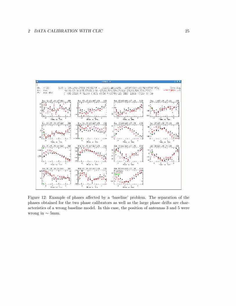
2 DATA CALIBRATION WITH CLIC 25
Figure 12: Example of phases affected by a ‘baseline’ problem. The separation of thephases obtained for the two phase calibrators as well as the large phase drifts are char-acteristics of a wrong baseline model. In this case, the position of antennas 3 and 5 werewrong in ∼ 5mm.

2 DATA CALIBRATION WITH CLIC 26
Figure 13: Example of a RF calibration where we can appreciate a remaining delay inthe baselines including A2. Delays can be solved with the commands “solve delay” and“modify delay” (see Sect. 2.6.9).

2 DATA CALIBRATION WITH CLIC 27
concerned scans must be selected with “find” and then the command “modify delay ...”must be typed, as proposed by the solution. After correcting delays the RF calibrationmust be repeated.
Note that, for the time being, the continuum units are not corrected offline for delays.If delays are modified, we advise using spectral units (instead of continuum ones) at eachstep of the calibration process.
Atmospheric Phase CorrectionBy default the atmospheric phase correction derived from the 22GHz receivers is
applied according to the results obtained with the PhCor procedure. We can howeverremove it by typing “let do atm no” in the line of commands before performing anycalibration. If a previous calibration was already carried out applying the atmosphericphase correction, the option no must be also selected in Use previous settings. Thewhole calibration must be then repeated. On the upper-left corner of each data plot wecan see Ph: Abs./Rel(A). Atm, where Atm reports on the presence of the atmosphericphase correction (according to PhCor).
See additional information in Sect. 2.6.3.
Several telescope configurationsIf a track includes observations with different telescope configurations, for example if
an antenna was removed during the observations, after clicking on Select the differentconfigurations will appear in the main calibration widget. The calibration must beperform independently for each configuration. Use previous settings is then set off.
2.6.10 FAQ
• How to proceed to repeat a calibration step? If you want to repeat a part of thecalibration, you do not need to repeat all the calibration steps happening before, butthose taking place later according to the scheme here described. Note that clickingon Select (within the Standard Calibration widget) is always recommended beforerepeating any calibration step, in order to have proper settings.
• How can I mask flagged data? Sometimes procedures crash because a lot of data of anantenna or baseline are flagged. We can verify the kind of flags with the command “list/flag”. We can mask them with the command “mask flag label /ant i” (or “/baselineij”). For example, “mask shadow /ant 3” would mask the flags of antenna 3 (logical)due to shadowing. Masking flags without a clear understanding of what it means is notrecommended. However, masking certain calibrator flags may be convenient in somecases (see Sect. 2.6.4, 2.6.5 and 2.6.7). If flagged data are masked in some part of thecalibration, the masking should be reset with “mask /reset” (e.g. “mask shadow /ant 3/reset”) at the end of the calibration step.

2 DATA CALIBRATION WITH CLIC 28
• Is there any command in clic that refers to physical antennas? No. The physicalantenna numbers are just shown in the plots of the First Look procedures, becausethe command “plot /physical” is the default there. Otherwise, all clic commands andprocedures use the logical numbers for antennas. This must be taken into account if AoDnotes refer to physical antennas, or when applying a new baseline model in observationswith an incomplete array.
• How can I flag data? After selecting the data to be flagged with “find”, you can usethe command “store flag flag label /ant i” (or “/baseline ij”). We can also delete themby changing their quality with the command “store quality 9 /ant i” (or “/baseline ij”).Please, ask your local contact if any doubt.
For example, the following commands would allow flagging correlations obtainedwith all antennas on a source of name starting by 1823, between the scans 234 and 250,with the label “redu”:CLIC> find /proc corr flux /sou 1823* /scan 234 250CLIC> store flag redu /ant all
2.6.11 Other calibration procedures
Baseline-based calibration
Sometimes we have difficulties to have antenna-based calibration solutions. In almostall the cases this can be solved by finding the origin of the problem, often due to thepresence of corrupted data. If the difficulties are found to be due to baseline-dependentproblems, for instance related to the correlator, to the atmosphere, etc, it may be betterto calibrate in baseline-based mode. In that case the hpb file must be created by usingthe clic command “copy header base” instead of “copy header antenna” (the default inSect. 2.4). The baseline-based solution can be then obtained by defining “set rf/ phase/amplitude baseline” before solving and storing. Antenna-based solutions can be alsostored in these hpb files by using “set rf/ phase/ amplitude antenna”, followed by solveand store. Note that the last solution stored is the one considered by default. Get incontact with your local contact for a more detailed explanation if needed.
Self-calibration
Self-calibration can be performed by selecting “Self-cal on point source” in the clicmenu (Fig. 1), with a procedure similar to that here described for a “Standard Calibra-tion” that includes also the source correlations.
2 DATA CALIBRATION WITH CLIC 29
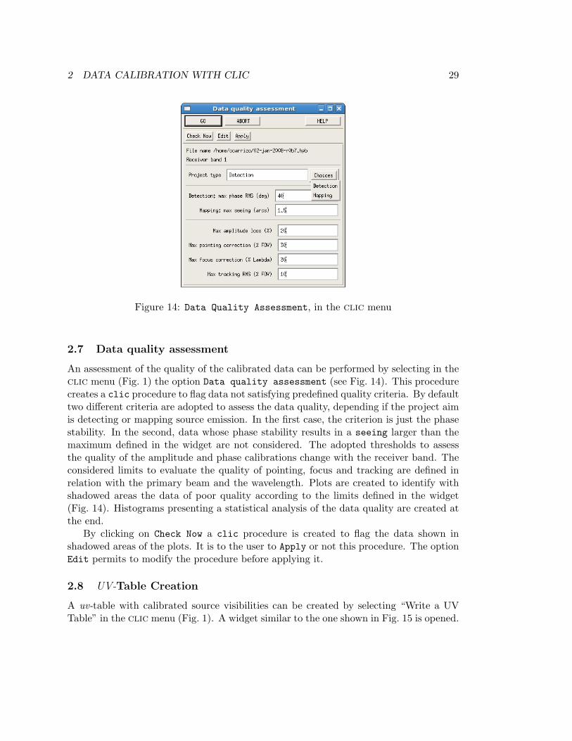
Figure 14: Data Quality Assessment, in the clic menu
2.7 Data quality assessment
An assessment of the quality of the calibrated data can be performed by selecting in theclic menu (Fig. 1) the option Data quality assessment (see Fig. 14). This procedurecreates a clic procedure to flag data not satisfying predefined quality criteria. By defaulttwo different criteria are adopted to assess the data quality, depending if the project aimis detecting or mapping source emission. In the first case, the criterion is just the phasestability. In the second, data whose phase stability results in a seeing larger than themaximum defined in the widget are not considered. The adopted thresholds to assessthe quality of the amplitude and phase calibrations change with the receiver band. Theconsidered limits to evaluate the quality of pointing, focus and tracking are defined inrelation with the primary beam and the wavelength. Plots are created to identify withshadowed areas the data of poor quality according to the limits defined in the widget(Fig. 14). Histograms presenting a statistical analysis of the data quality are created atthe end.
By clicking on Check Now a clic procedure is created to flag the data shown inshadowed areas of the plots. It is to the user to Apply or not this procedure. The optionEdit permits to modify the procedure before applying it.
2.8 UV-Table Creation
A uv-table with calibrated source visibilities can be created by selecting “Write a UVTable” in the clic menu (Fig. 1). A widget similar to the one shown in Fig. 15 is opened.

2 DATA CALIBRATION WITH CLIC 30
Figure 15: Write a UV Table, in the clic menu.
The hpb file name, table name (with no extension), source name, receiver band, tunedside band and table mode (with spectral -LINE- or without spectral -CONT- information)are to be specified. In the widget, the atmospheric phase correction must be disabled ifit was not taken into account in the calibration. The rest frequency can be redefined,as well as the table resampling for the LINE mode. A uv-table is newly created if theoption New Table is set on; visibilities are added to an existing uv-table if the optionNew Table is set off.
This procedure creates (or includes) the selected calibrated source visibilities into thespecified uv-table, but also creates (or updates) a clic procedure, which can be executedby entering “@mytable-table.clic” in clic to produce the same table (of name “mytable”in this example). Editing a script to create tables (the file “mytable-table.clic” in ourexample, see Fig. 16) is easy and likely faster than filling in all the options available in thewidget to create tables. This clic procedure defines the hpb file, calibration and tablesettings, selects the correlations on source, and finally uses the clic command “table”,possibly with the options “/resample” and “/frequency”. In the clic menu there existother more complex procedures to create tables, but likely none of them is as fast and

2 DATA CALIBRATION WITH CLIC 31
flexible as editing table scripts is.Particularly for mosaics a table must be created for each observed offset, all of them
with a generic common name followed by an offset number (an example is shown in Fig.16). The imaging mapping procedures (presented in Sect. 3) will so recognize the mosaicand properly proceed with the imaging.
2.9 Calibrating and/or merging with data previous to 2007
2.9.1 clic backwards compatible
The current versions of clic are backwards compatible and hence can be also used tocalibrate data obtained before 2007, when a new generation of receivers was installed atPlateau de Bure (see also Sect. 2.9.5).
2.9.2 uv-tables obtained before 04/2004
The format of the uv-tables changed in March 30, 2004. The mapping command“uvt convert” updates the uv-tables’ format to be treated with a recent GILDAS ver-sion and particularly to mix the old tables with recent data.
2.9.3 Merging old and new data
In order to merge old and new data the best is likely to create the uv-tables from theold and the new hpb files, with the same CLIC version dated later than April 2004, asdescribed in Sect. 2.8: 1) Using the widget to create a table or just to add visibilities ina previous table by setting on or off the option New table (see Fig. 15). 2) Editing atable script and using the command table with the options new and/or old as shown inFig. 16, depending if the table is to be created or if just visibilities from a second dataset are added.
Otherwise, uv-tables can be merged with the procedure “run uv merge” either inclic or in mapping, provided they have the same spectral setup. Contact your localcontact if your situation does not correspond to any of the mentioned cases.
2.9.4 Continuum projects between 11/2005 and 01/2007
In November 25, 2005, prototypes of the new generation of receivers were installed onantenna 6, while the other antennas continued observing with the old receivers. Thissituation remained until January 2007, when all antennas were equipped with new re-ceivers. As a consequence, for those projects observed with DSB tuning the creation ofcontinuum tables from all baselines except for those with antenna 6 should be made byusing both bands, but the baselines with antenna 6 should just include the tuned band(pure SSB). Note that this affects all 1mm continuum projects, where the tuning wasDSB by default with the old receivers.

2 DATA CALIBRATION WITH CLIC 32
Figure 16: Script to create uv-tables for a mosaic of two points, as edited by emacs. Notethat for the data of the second day the same settings adopted but for the atmosphericphase correction and the considered scan range.
To create continuum tables we recommend: First, storing in the uv-table thedata coming from all the antennas for the band tuned in antenna 6. Second, storingthe visibilities obtained for the other band, ignoring antenna 6 data. For example,for a project LSB tuned in antenna 6, but DSB in the others, we would proceed as follows:
set band lsbtable table nameset band usbmark data /ant 6table table name /nocheck scan

2 DATA CALIBRATION WITH CLIC 33
2.9.5 Very Old Projects
The calibration of very old projects (older ∼ 1995) is likely not possible with widgetsbecause of the many big changes over the years. Consult the SOG (at [email protected]) ifneeded.

3 FIRST INSTRUCTIONS FOR DATA ANALYSIS WITH MAPPING 34
3 First Instructions for Data Analysis with MAPPING
mapping is the GILDAS software package to image and analyze NOEMA data. Thetools described here are complex procedures built over simple mapping commands. Werecommend to look at the mapping manual to have a deeper understanding of imagingand deconvolution concepts and of the command functionalities.
Figure 17: mapping menu.
The menu shown in Fig. 17 leads to two main sections, Operations on UV-tablesand Imaging and deconvolution. In the widgets resulting from the selection of theseoptions (Figs. 18 and 21) the left column lists the procedures to be run, their controlparameters can be edited by clicking on the related button in the central column, helpis displayed by pushing on the right buttons. At the bottom of all the “Parameters”widgets (see e.g. Fig. 19 and 20) there are the options GO and DISMISS. GO executes theprocedure with the specified parameters, DISMISS closes the widget.
In the below sections, the paragraphs starting with At the prompt: describe howto run the same procedures through the command line instead of through the widgets.While this possibility exists for all the widget functionalities, information is given for someof them. In general, typing“go procedure name” is needed to call mapping procedures.To modify the control parameters “let variable name value” is used. Their content canbe checked with “input procedure name” or by typing “exam variable name”. The nameand a short description of the control variables can be found by clicking where the valuesfor parameters are requested, in the widgets.
In addition, a few variables are used by (almost) all the procedures. You can alsodefine their values directly at the prompt. For instance “let name ...” is used to definethe generic name (without extension) of your table or image, “let first ...” to definethe first channel to be considered, “let last ...” to define the last one.
3.1 Operations on UV table
By clicking in the mapping menu (Fig. 17) on Operations on UV table the widgetpresented in Fig. 18 is opened. There, by clicking on the buttons in the column on the
3 FIRST INSTRUCTIONS FOR DATA ANALYSIS WITH MAPPING 35
left, we run the corresponding procedures, some of them described below. We stronglyrecommend to look at the adopted parameters (in the central column) before executingthem.
The main procedures related to the analysis of the data in the uv-plane are describedin the following sections:
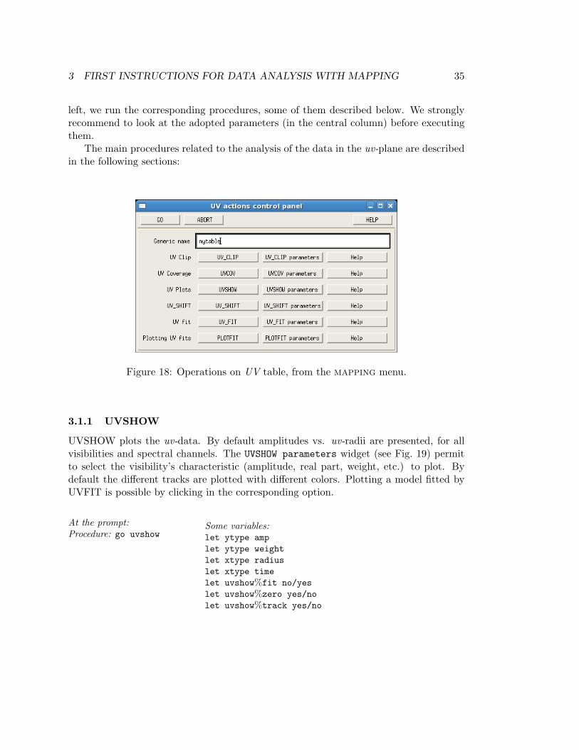
Figure 18: Operations on UV table, from the mapping menu.
3.1.1 UVSHOW
UVSHOW plots the uv-data. By default amplitudes vs. uv-radii are presented, for allvisibilities and spectral channels. The UVSHOW parameters widget (see Fig. 19) permitto select the visibility’s characteristic (amplitude, real part, weight, etc.) to plot. Bydefault the different tracks are plotted with different colors. Plotting a model fitted byUVFIT is possible by clicking in the corresponding option.
At the prompt:Procedure: go uvshow
Some variables:let ytype amplet ytype weightlet xtype radiuslet xtype timelet uvshow%fit no/yeslet uvshow%zero yes/nolet uvshow%track yes/no

3 FIRST INSTRUCTIONS FOR DATA ANALYSIS WITH MAPPING 36
Figure 19: UVSHOW parameters, to plot the UV-data.
3.1.2 UVSHIFT
Procedure to shift the phase center of a UV-table. Absolute or relative coordinates canbe introduced. The position angle of the reference axes (which is then considered by theplotting procedures) can also be changed.
At the prompt:Procedure: go uv shift
3.1.3 UVFIT
Procedure to fit the obtained uv-data with the Fourier Transform of the following func-tions (see Fig. 20): a point, a circular Gaussian, an elliptical Gaussian, a circular disk,an elliptical disk, a circular or elliptical ring, an exponential brightness distribution, adistribution proportional to radius−2, and a distribution proportional to radius−3. Someparameters can be fixed by defining them in the option Parameters. They are the offsetR.A., offset Dec and flux for a point function, offset R.A., offset Dec, flux and diameterfor c gauss, offset R.A., offset Dec, flux, major and minor diameter and position angle fore gauss, offset R.A., offset Dec, flux and diameter for c disk, offset R.A., offset Dec, flux,major and minor diameter and position angle for e disk, offset R.A., offset Dec, flux,

3 FIRST INSTRUCTIONS FOR DATA ANALYSIS WITH MAPPING 37
inner diameter and outer diameter for a ring, offset R.A., offset Dec, flux and diameterfor the functions called expo, power-2 and power-3.
The fitted function can be subtracted in a residual table (of extension uvfit) thatlater can be plotted with UVSHOW (Sect. 3.1.1).
Figure 20: Left: UV FIT parameters, to fit the UV-data with the Fourier Transform ofsimple functions. Right: PLOTFIT parameters, to plot the fitting results obtained withUVFIT.
3.1.4 PLOTFIT
PLOTFIT is aimed to plot the results of UVFIT. The number of parameters to plot (seeFig. 20) is to be defined if larger than 3. By default it presents the position of the centerof the fitted function, R.A. and Dec, and the flux at each velocity. Several options areavailable for each fitting. Error bars are plotted by default.
3 FIRST INSTRUCTIONS FOR DATA ANALYSIS WITH MAPPING 38
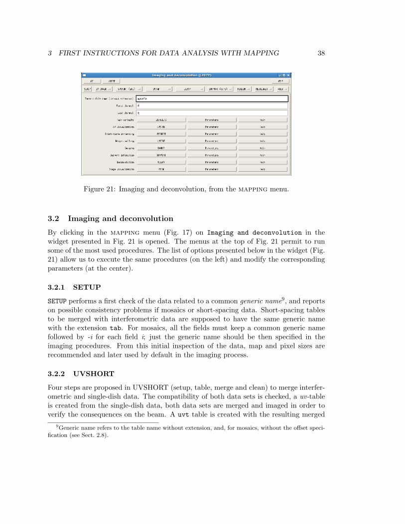
Figure 21: Imaging and deconvolution, from the mapping menu.
3.2 Imaging and deconvolution
By clicking in the mapping menu (Fig. 17) on Imaging and deconvolution in thewidget presented in Fig. 21 is opened. The menus at the top of Fig. 21 permit to runsome of the most used procedures. The list of options presented below in the widget (Fig.21) allow us to execute the same procedures (on the left) and modify the correspondingparameters (at the center).
3.2.1 SETUP
SETUP performs a first check of the data related to a common generic name9, and reportson possible consistency problems if mosaics or short-spacing data. Short-spacing tablesto be merged with interferometric data are supposed to have the same generic namewith the extension tab. For mosaics, all the fields must keep a common generic namefollowed by -i for each field i; just the generic name should be then specified in theimaging procedures. From this initial inspection of the data, map and pixel sizes arerecommended and later used by default in the imaging process.
3.2.2 UVSHORT
Four steps are proposed in UVSHORT (setup, table, merge and clean) to merge interfer-ometric and single-dish data. The compatibility of both data sets is checked, a uv-tableis created from the single-dish data, both data sets are merged and imaged in order toverify the consequences on the beam. A uvt table is created with the resulting merged
9Generic name refers to the table name without extension, and, for mosaics, without the offset speci-fication (see Sect. 2.8).

3 FIRST INSTRUCTIONS FOR DATA ANALYSIS WITH MAPPING 39
data. The default UVSHORT parameters are well adapted for merging NOEMA and30m-telescope data.
We recommend to use the procedure UVSHOW (see Sect. 3.1.1) to verify the mergeduv data, and particularly to verify that the flux calibration is not incompatible. Forexample, by plotting amplitude versus uv radius we can check the flux of both data setsat their interface, i.e. at a uv radius of 15m (for the NOEMA array).
3.2.3 UVMAP
Procedure to compute a dirty map (with extension lmv) and beam (with extension beam)from uv-tables. For mosaics a unique dirty image is created, as well as individual onesfor each field. UVMAP estimates which are the best values for pixel and map sizes. Werecommend to use them. By default images are created by using natural weights forthe visibilities. Uniform weights can be defined in the widget (see Fig. 22), but indeedcorrespond to robust weighting.
Figure 22: UVMAP parameters, to create a dirty (.lmv) image.
UVSTAT weight/taper The advantages and inconveniences of modifying the weightsfrom natural to robust are quantified, and numbers are shown by UVSTAT in modeweight. The advantages and inconveniences of tapering can be verified with UVSTAT

3 FIRST INSTRUCTIONS FOR DATA ANALYSIS WITH MAPPING 40
in mode taper.
DIRTY/BEAM/PRIMARY/WEIGHTS at the top of the imaging widget (Fig. 21)are aimed to plot the results from UVMAP, that is “mytable”.lmv, “mytable”.beam, and,if mosaicing, also “mytable”.lobe and “mytable”.weight.
At the prompt:Procedure: go uv map
To plot:Procedure: go bit
Some variables:let type lmvlet type beamlet first 7
3.2.4 SUPPORT
Procedure to define polygons inside which the CLEANing procedure will look for CLEANcomponents. A common polygon can be defined for all the channels, or one polygonper channel. Polygons can be defined with the cursor or by introducing the neededparameters to define elliptical or rectangular supports. All these possibilities can beeasily identified in the SUPPORT widget.
At the prompt:Procedure: go support
Some variables:let support%oneperplane yes/nolet support%kind cursor/ellipse/rect
3.2.5 CLEAN
It identifies in the dirty map CLEAN components and convolve them with a deducedsynthetic beam. Different CLEANing methods can be used. HOGBOM and CLARKare recommended for being the most robust (see MAPPING manual for details). By usingSUPPORTs the search for CLEAN components can be restricted to the areas where thesource is known to be (when the variable myclean%support=yes, see Sect. 3.2.4). Thecriterion to stop the search for CLEAN components within the residual map can bemodified by changing the Stopping criteria options in the CLEAN parameters widget(Fig. 23). By default no supports are used in a first CLEANing of a dirty map, but canbe defined for later CLEANing. The option to CLEAN with supports can also be seton or off in the CLEAN parameters widget. By default the flux accumulated in the

3 FIRST INSTRUCTIONS FOR DATA ANALYSIS WITH MAPPING 41
identified CLEAN components is shown (if myclean%show=yes), and stored in a file ofname including -cct.
Figure 23: Clean parameters, to identify CLEAN components and convolve them withthe deduced synthetic beam.
HOGBOM/CLARK/others at the top of the imaging widget permits CLEANing byusing the defined parameters.
RESIDUALS/CLEAN/CCT at the top of the imaging widget plots the resultingresiduals (stored in a file of extension .lmv-res), the CLEANed image (in a file of ex-tension .lmv-clean) or the found CLEAN components (in a file of extension .lmv-cct).
3 FIRST INSTRUCTIONS FOR DATA ANALYSIS WITH MAPPING 42
At the prompt:Procedure: go clean
Some variables:let method hogbom/clarklet myclean%show yes/nolet myclean%support yes/nolet niter 1500let ares 1e-3
To plot:Procedure: go bit
Some variables:let type lmv-cleanlet first 23let last 45let type lmv-res
3.2.6 VIEW
Procedure to plot resulting images and cubes. VIEW plots the averaged image, a selectedchannel, the line profile obtained from a certain position, and the integrated line profile.Ranges and channels to plot, and areas and pixels for which profiles should be shown,are selected by clicking on each plot with the mouse. Typing h anywhere in the plottingwindow displays help information on the terminal. BIT presents the images obtained forall the spectral channels (within the specified first and last channels)
VIEW/BIT at the top of the imaging widget permits selecting the procedure to plot.
At the prompt:Procedure: go view
Procedure: go bit Some variables:let type lmv-cleanlet first 23let last 45let size 50let spacing 3e-3

A APPENDIX: CALIBRATION PRINCIPLES 43
A Appendix: Calibration Principles
An “ideal” interferometer samples the Fourier transform of the sky brightness multipliedby the antenna beam pattern; these samples are called visibilities. In practice, becauseof noise, imperfections, sampling, and other effects, several terms perturb the visibilitiesto produce the true output of a “real” interferometer. The goal of the calibration is toidentify and estimate all the important instrumental and atmospheric effects and applyappropriate corrections to recover the true visibilities.
A.1 Standard Decomposition of Visibilities
For any given complex number Z, let us call PZ its phase, AZ its amplitude, and Z∗
its complex conjugate. The observed visibility Vijk(t) is a complex number representingthe amplitude and phase of the signal detected on baseline ij, from spectral channel k,at time t,
Vijk(t) = AVijk(t). exp(−i.PVijk(t)) (1)
This visibility is the Fourier transform of the product of the primary beam patternsof the antennas and the brightness distribution of the observed source, sampled at thepoint (u(t), v(t))ij corresponding to baseline ij at time t,
Vijk(t) = FT (Bi(x, y, x0 + xi, y0 + yi)B∗j (x, y, x0 + xj , y0 + yj)I(x, y, k))(u, v)ij (2)
where
• FT is the Fourier Transform operation, x, y are integration parameters,
• I(x, y, k) is the brightness distribution of the source at frequency k,
• Bi(x, y, x′, y′) is the voltage pattern of antenna i pointed in direction (x′, y′),
• (x0, y0) is the pointing direction of the antennas,
• (xi, yi) is the pointing error of antenna i, and
• (u, v)ij are the projected coordinates of baseline ij, in wavelength units.
If we further assume that all antennas are equal, their pointing errors are negligible, theirbeam shape does not depend on the pointing direction, and the fractional bandwidth issmall (δν/ν << 1), this equation reduces to
Vijk(t) = FT (P (x, y)I(x, y, k))(u, v)ij (3)
where P (x, y) is the power beam pattern of the antennas.

A APPENDIX: CALIBRATION PRINCIPLES 44
The antennas, receivers, cables, and correlators all introduce additional modificationsto this visibility. These perturbations can be formally decomposed into
Vijk = AiA∗jSikS
∗jkCijkRijk +Oijk +Nijk (4)
where
• Ai is the complex gain of antenna i (amplitude and phase),
• Sik is the complex gain of channel k for antenna i,
• Cijk is the complex gain of channel k for correlator entry ij,
• Rijk is the theoretical visibility of the source,
• Oijk is a non random error on channel k for correlator entry ij. These errors havevarious origins, such as finite bandpass, bandpass mismatch between antennas iand j, etc...), and
• Nijk is a random error due to detection noise.
Provided the design of the interferometer system is adequate, the terms appearing inthis decomposition have the following properties:
• Nijk(t) is normally distributed with known variance.
• Oijk is negligible with respect to Nijk. We will assume Oijk = 0 in the followingdiscussion.
• Cijk(t) is only weakly time dependent. This factor is introduced essentially by ana-log filters in the correlator and residual (constant) delay offsets between subbands;it may depend strongly on k.
• Sik(t) is only weakly time dependent. This factor is introduced by receivers andIF cables. The frequency (k) dependence is weak.
• Ai(t) depends on antenna pointing (amplitude only), focus (amplitude and phase),and on atmosphere (amplitude and phase).
Let W = V −O −N = V −N to first order. Here, PNijk(t) is a random phase andANijk(t) has known variance, <AN>. Then
PWijk(t) = PAi(t) + PSik(t)− PAj(t)− PSjk(t) + PCijk(t) + PRijk(t) (5)
PWijk(t) = PVijk(t) + PDijk(t) (6)
where

A APPENDIX: CALIBRATION PRINCIPLES 45
• PAi is the instrumental phase on antenna i
• PSik is the relative phase of channel k for antenna i
• PCijk is the relative phase of channel k for correlator entry ij, independent of thePSik
• PRijk is the source phase on baseline ij for channel k. Rijk(t) only depends on ijthrough the coordinates of antennas i and j, via (u(t), v(t))ij .
• PDijk is a phase noise introduced by measurement noise Nijk
Then, to first order,
• PCijk can be measured independently, and is only weakly time dependent,
• PSik is constant, providing the receiver is not retuned,
• PAi is time variable, on many different timescales, and
• PDijk has known variance, depending on Wijk/<AN>.
Similar relations can be expressed for the intensities:
AWijk(t) = AAi(t).ASik(t).AAj(t).ASjk(t)).ACijk(t).ARijk(t) (7)
andAWijk(t) = AVijk(t) +ADijk(t) (8)
where
• AAi is the gain of antenna i (including effects due to atmospheric absorption, focus,receiver gain, pointing, etc...),
• ASik is the relative gain of channel k for antenna i,
• ACijk is the relative gain of channel k for correlator entry i, j, measured indepen-dently from ASik,
• ARijk is the Source intensity on baseline ij. ARijk(t) depends on ij only throughantenna coordinates.
• ADijk has known variance <AN>.
The purpose of calibration is to determine as best as possible these various func-tions, taking advantage of the time independence of some parameters, and of the weakchromaticity of the atmosphere.

A APPENDIX: CALIBRATION PRINCIPLES 46
A.2 Baseline versus Antenna based calibration
Although many of these calibration parameters are antenna based, clic is able to keepsimultaneously two values for these parameters: an antenna-based value and a baseline-based value. Whenever an antenna-based calibration function is computed (i.e. a partof the Ai, or of the Sij), clic offers the possibility of solving for an antenna-based ora baseline-based function. In general, solving for antenna based parameters should bepreferred, since this mode offers less free parameters (so that they are better constrained)and uses a priori knowledge of the instrument (e.g. the phase closure relations). However,in some cases, well-identified baseline-related problems make it difficult to calibrate inantenna-based mode, so it may be needed to look for baseline-based solutions, mainlyfor amplitude or phase calibration.
A.3 Plateau de Bure Online Calibration
Some of the mentioned terms are partially estimated on real time so that the storedvisibilities are already corrected from their contribution. Specific OBS commands, adedicated GILDAS software package (RDI) and some clic procedures are used to produceand reduce the following scans:
• CALI: Each scan consists of two or three subscans, obtained by the OBS com-mand CALIBRATE. They are used to measure the atmospheric transmission andreceiver temperature, converting backend counts in antenna temperature outsideatmosphere (which is a factor in AAi, excluding pointing and focus terms).
• IFPB: Two subscans are obtained by the OBS command BANDPASS, whichswitches the correlator entries to a common noise source. Thus all the ACijk
and PCijk are measured, except for a residual delay (visible as a constant phaseslope with respect to frequency) due to path differences between the noise sourceand the antenna connections to the correlator.
• GAIN: This procedure allows measuring the sideband gain ratio of the receivers,by looking at a strong cosmic source (in practice, only AIi is computed, althoughthe phase term PIi could also be derived). Since this ratio only depends on thereceiver tuning, in particular on the backshort tuning, a CALIBRATE scan is madejust after tuning modifications.
Results from CALI and IFPB observations are applied to the data by the automaticdata compression job. Corrections from tuning modifications are introduced in OBS bythe operator just after GAIN, at the beginning of the observations. Therefore, in principle,amplitude errors should only be due to phase noise, pointing and focus errors.

A APPENDIX: CALIBRATION PRINCIPLES 47
A.4 Offline Calibration; the rules of the game
The purpose of the offline calibration (carried out when the acquisition process is endedat the observatory) is to estimate as precisely as possible all the various terms of Equa-tion 4. The basic principle is to measure the visibilities of sources with known (spatialand frequency) structure, in practice continuum point-like sources (called calibrators),which flux (so bijk) is also known or can be deduced. By simple division, the productAi.A
∗j .Sij .S
∗ij is determined at the time intervals in which these calibrators are observed,
and interpolated for the intermediate times in which the project source is. The signal tonoise ratio of the calibrator measurements is the main limiting factor in this process.
Another important limitation concerns the validity of the interpolations used to pre-dict the values of the calibration factors on the studied sources. It is desirable to estimatethe quality of these predictions, and to ignore data which for any reason may deviatesubstantially from the predictions (for example due to instrumental problems, strongatmospheric variations, etc).
B APPENDIX: PIPELINE OR AOD FIRST LOOK 48
B Appendix: Pipeline or AoD First Look
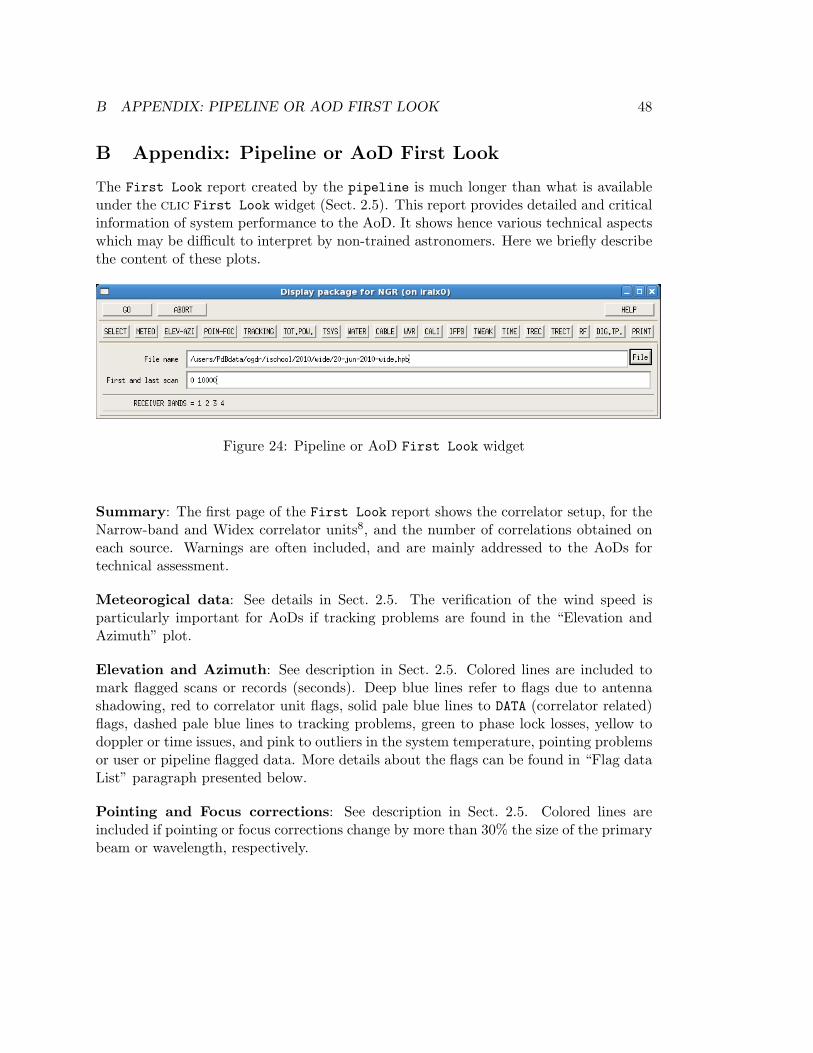
The First Look report created by the pipeline is much longer than what is availableunder the clic First Look widget (Sect. 2.5). This report provides detailed and criticalinformation of system performance to the AoD. It shows hence various technical aspectswhich may be difficult to interpret by non-trained astronomers. Here we briefly describethe content of these plots.
Figure 24: Pipeline or AoD First Look widget
Summary: The first page of the First Look report shows the correlator setup, for theNarrow-band and Widex correlator units8, and the number of correlations obtained oneach source. Warnings are often included, and are mainly addressed to the AoDs fortechnical assessment.
Meteorogical data: See details in Sect. 2.5. The verification of the wind speed isparticularly important for AoDs if tracking problems are found in the “Elevation andAzimuth” plot.
Elevation and Azimuth: See description in Sect. 2.5. Colored lines are included tomark flagged scans or records (seconds). Deep blue lines refer to flags due to antennashadowing, red to correlator unit flags, solid pale blue lines to DATA (correlator related)flags, dashed pale blue lines to tracking problems, green to phase lock losses, yellow todoppler or time issues, and pink to outliers in the system temperature, pointing problemsor user or pipeline flagged data. More details about the flags can be found in “Flag dataList” paragraph presented below.
Pointing and Focus corrections: See description in Sect. 2.5. Colored lines areincluded if pointing or focus corrections change by more than 30% the size of the primarybeam or wavelength, respectively.
B APPENDIX: PIPELINE OR AOD FIRST LOOK 49
Antenna Tracking Errors: See description in Sect. 2.5. Problems are often relatedto strong wind. It may happen, though it remains very rare, that large tracking er-rors indicate a technical problem. This monitoring is particularly important to foreseeinterventions by the technical staff in NOEMA antennas.
22GHz monitors present the results obtained in time from the 22GHz receiver in eachantenna. The first three plots show the counts obtained in each of the three channels ofthe 22GHz receivers. They are combined to produce the ‘triple’ values, which are usedto model the atmosphere, disentangle between water vapor and droplets, and predictthe atmospheric phase fluctuations by which the interferometric data are affected. Thisis then used to reduce of phase decorrelation within each scan. Derived water vaporamounts are displayed in the ‘Water Monitoring’ plots. The given ambient temperaturesare obtained by sensors placed close to the 22GHz receivers. Peltier Temperatures aredirectly related to the receiver performance, and should remain within the plot limits.
CALI scans vs time plots show the time evolution of the CALI autocorrelation scans,which can consist of two (on the hot load and sky respectively) or three (on the cold load,hot load and sky) subscans. Measurements on the cold load are typically performed every∼ 50 min, and are used to derive and monitor receiver temperatures. Differences betweenantennas are normally linked to receiver attenuations, and differences between units areoften linked to correlator tweaks. In correct weather conditions, the sky autocorrelationsshow a constant value because the signal variations due to airmass change is compensatedby correlator tweaking. This tweaking effect is however visible in the autocorrelationson the loads. (Note that Widex tweak levels change in large steps.) Strong variations inthe input signal often result in changes in the tweak values, and accordingly in the CALIautocorrelations.
IFPB scans vs time plots present the time evolution of the amplitudes of the IFPBcorrelations obtained on the noise source (see Sect. 2.2). Absolute amplitude valueschange from unit to unit, depending on the IF phase delay. As the noise diode provides aconstant input, IFPB amplitudes should remain constant along a track. Sharp variationsin the tweak levels (for instance due to bad weather) can however result in changingamplitudes of the IFPB scans, due to tweaking adjustment effects.
Tweak levels vs time plots show the tweak levels for each of the Narrow correlatorunits, per correlator sub-band. Values remaining constant (in correct weather conditions)in time correspond to the IFPB scans, tweak values change with the airmass for the otheracquisitions.
Monitoring the time, UTC, NTP and PPS. The monitoring of the time synchro-nization signals is important as it is essential to stop fringes, ensure a good pointing,
B APPENDIX: PIPELINE OR AOD FIRST LOOK 50
etc. This plot helps us to monitor differences in time between the UTC (from the maser-synchronized GPS) and NTP ([GPS-]synchronized NTP) times, as well as time offsetsbetween hardware clocks (PPS used by the correlator from maser-synchronized GPStime) and software synchronized events (NTP).
Receiver Temperatures in the IF plots present the receiver temperature computedalong the IF bandwidth from one of the first CALI scans including a cold load acquisition(often called ‘cal-cold’ scan). Different colors are used to identify the different correlatorinputs. These plots shows better than any other the presence of parasites and tuningfeatures. Particularly, marks are included to identify the known system parasites (fromthe IF processor at 6300, 4500 MHz, and at 3 and 4 times the LO1ref local oscillatorfrequencies). Dotted lines represent the values stored in the data header, computed bythe online RDI software.
Receiver Temperatures vs Time plots display the evolution of the mean receivertemperature values averaged over the correlator-input8 bands. They should not changeby more than a few K in projects with stable tunings. Tunings affected by strong parasitesmay show changing receiver temperatures. An intervention from the frontend group mayhappen as a consequence of the information extracted from these plots.
Dewar Temperature plots show the temperatures measured at various stages in thecryostat.
Observing List summarizes the sequence of obtained scans. CALI and IFPB acquisitionsare ignored in this list.
Flagged data List shows all the flagged records and scans. It should be consistent withthe color marks in the ’Elevation-Azimuth’ plots.
Total Power vs time: See description in Sect. 2.5. Values are presented per eachcalibration unit (which correspond to correlator inputs8): Two Narrow Quarters andfour Widex units. Moderate differences (of a few K) in the values from the differentunits are due to the different covered frequency ranges.
Cable Phase plots present the phase delays (in degrees) produced at the Master Fre-quency level by the cables in their movements, mostly due to antenna tracking, for theused and unused bands. Colored lines mark changes that could result in phase variationslarger than 30o. Significant changes in the LO1ref local oscillator frequencies are alsodisplayed in grey lines.
System Temperatures vs time: See description in Sect. 2.5. Plots are shown percalibration unit.

B APPENDIX: PIPELINE OR AOD FIRST LOOK 51
Water Vapor vs time: See first description in Sect. 2.5. A plot is created per cali-bration unit. A differential plot is created to compare the results obtained from all theantennas. Pale blue lines in the WVR H2O plots mark the update of the 22GHz receivercalibration by the online software.
RF phases plots compare the phases obtained per correlator input in the (IF1) frequencyband. Remaining phase delays can be identified in these plots. One plot is created forthe first correlation scan at the project start, another for the last correlation scan at theproject end. Note that if the (frequency averaged) phases from H and V polarizationreceivers are not equal, “let phcal ‘*’ ” should be entered after Select (see Sects. 2.6.1and 2.6.5).
Amplitudes for Narrow and Widex correlator inputs: Comparison of the signallevel obtained from all the correlator inputs8 (or calibration units), which -in principle-should be almost identical. Uncorrected delays result in amplitude differences amongthe correlator units, which become particularly important between the Widex and theNarrow-band correlator units. Delays can be identified in the RF phases and the RFcalibration plots, and the data can be corrected for them by following the instructionsin Sect. 2.6.9.