1 23

Sports Engineering ISSN 1369-7072Volume 16Number 1 Sports Eng (2013) 16:29-41DOI 10.1007/s12283-012-0105-8

A mathematical analysis of the motion ofan in-flight soccer ball

T. G. Myers & S. L. Mitchell

1 23

Your article is protected by copyright and all

rights are held exclusively by International

Sports Engineering Association. This e-

offprint is for personal use only and shall not

be self-archived in electronic repositories.

If you wish to self-archive your work, please

use the accepted author’s version for posting

to your own website or your institution’s

repository. You may further deposit the

accepted author’s version on a funder’s

repository at a funder’s request, provided it is

not made publicly available until 12 months

after publication.

ORIGINAL ARTICLE

A mathematical analysis of the motion of an in-flight soccer ball

T. G. Myers • S. L. Mitchell

Published online: 16 October 2012

� International Sports Engineering Association 2012

Abstract In this paper, an analytical and numerical study

of the three-dimensional equations describing the motion

through the air of a spinning ball is presented. The initial

analysis involves constant drag coefficients, but is later

extended to involve drag varying with the spin ratio.

Excellent agreement is demonstrated between numerical,

analytical and experimental results. The analytical solution

shows explicitly how the ball’s motion depends on para-

meters such as ball roughness, velocity and atmospheric

conditions. The importance of applying three-dimensional

models, rather than two-dimensional approximations, is

demonstrated.

Keywords Aerodynamics � Soccer ball flight � Spinning

soccer ball � Magnus force � Perturbation solution

1 Introduction

Over the years much work has been carried out on football

design, moving from the traditional leather ball encasing an

inflated pig’s bladder to the most recent Jabulani which is

constructed using polyurethane panels. The goal of the

technological advances in football design has been to make

the ball more reliable and better to play with, for the benefit

of all players involved. Recently, at a mathematics in

industry study group held in Johannesburg, the coach of a

South African premiership team, Bidvest Wits, posed the

question of whether a match ball could be chosen to benefit

the home side (or alternatively disadvantage the visiting

team). This paper has evolved from that study and in the

conclusions the question of whether the ball choice can

indeed provide a home advantage will be discussed.

In professional football matches in South Africa, and

many other countries, the home team provides the ball. The

choice of ball is of course restricted, primarily by FIFA law

2, which dictates the size, (dry) weight, pressure and

material. Hence, the main changes in ball design have

entered through the material and shape of the panels [10].

A further restriction comes through the sponsor, in that the

team must use one of their balls. In the case of Bidvest

Wits the balls are provided by Nike. During the meeting in

Johannesburg three Nike balls were presented, the balls had

a very similar appearance; however, there was one signif-

icant difference in that two balls were rough (with dimpled

panels) while one ball had smooth panels (see, for example,

close-up pictures of the Nike T90 Tracer and Catalyst on

http://Nike.com).

To answer the question on the choice of ball, the fol-

lowing analysis will focus on its motion through the air and

in particular from a free kick or corner. One reason for this

is that these are relatively controlled situations and there is

much data on a ball’s motion through the air. A second

reason is that free kicks are an important factor in scoring:

in the 1998 world cup 42 of the 171 goals scored came

from set-plays, with 50 % of these from free kicks [2].

Consequently, understanding the ball motion through the

air from a free kick or corner could provide important

information concerning the best ball choice. A final reason

is that Johannesburg is located high above sea level (at

T. G. Myers

Centre de Recerca Matematica, Campus de Bellaterra,

Edifici C, Bellaterra, 08193 Barcelona, Spain

e-mail: tmyers@crm.cat

S. L. Mitchell (&)

MACSI, Department of Mathematics and Statistics,

University of Limerick, Limerick, Ireland

e-mail: sarah.mitchell@ul.ie

Sports Eng (2013) 16:29–41

DOI 10.1007/s12283-012-0105-8

Author's personal copy

around 1,800 m). The air density is approximately 20 %

lower than that at sea level [11] and so it is expected that

the greatest difference in ball motion between Johannes-

burg and cities located at a lower altitude will be when it

moves through the air.

Of course there has been much work carried out on

the motion of balls and projectiles through the air. As

early as the 1600s Newton noted that a spinning tennis

ball had a curved trajectory. A century later, Robin

showed there was a transverse aerodynamic force on a

rotating sphere: this is what is now termed the Magnus

effect (or more fairly the Robin–Magnus effect). In the

late 1800s Tait was the first to apply this notion to a

sports ball (unfortunately, a golf ball rather than a

football). All of this work involved frictionless fluids and

so the correct explanation for the Magnus effect had to

wait until Prandtl’s boundary layer theory of 1904.

Specific analysis of the motion of an in-flight football

came much later. Asai et al. [1] carried out an experi-

mental study of the lift coefficients on a spinning and

non-spinning football and showed a strong dependence

on the lift coefficient with spin rate. The equations of

motion for a football are provided in many papers;

however, the convention of Goff and Carre [7] is used in

this study, where the Magnus effect is split into lift and

lateral components (Asai et al. also work with two

components). Horzer et al. [11] provide useful details of

the differences in atmospheric conditions between World

Cup venues in South Africa and demonstrate the effect

of altitude on a ball’s trajectory. Oggiano and Sætran

[14] compare the trajectory of different footballs: this

confirmed the belief that the ball choice could provide a

home advantage.

The organisation of this paper is as follows. In Sect. 2

the three-dimensional mathematical model is given, this is

well established and simply involves Newton’s second law.

Due to the nonlinearity of the governing equations, all

previous solutions have been obtained numerically. In an

analysis of a simpler model than that considered in the

present study, Bray and Kerwin [2] state that the governing

equations have no closed form solution, although this is

technically correct an accurate approximate solution is

derived in Sect. 3. This clearly shows the effect of the

model parameters on the ball’s motion, which is not pos-

sible with a numerical solution. In Sect. 4 numerical

solutions are calculated to verify the accuracy of the

approximate solution. Experimental studies on drag and lift

coefficients have demonstrated their dependence on spin,

however, theoretical studies generally set the coefficients

as constant. In Sect. 5 the analysis is extended to deal with

variable coefficients. Finally, the question of whether the

choice of ball can really provide a home advantage is

discussed.

2 Mathematical model

The motion of a football is described by Newton’s second

law F ¼ m€x; where the force F comprises gravity and drag

due to the air. For a non-spinning ball the drag force acts

solely in the direction opposite to the ball’s motion. For a

spinning ball the drag has two components, the resistance

opposing forward motion and the Magnus force. The

Magnus force acts perpendicular to the direction of motion

and the spin axis. This force may be resolved into two

components denoting lift and lateral motion (see [1, 7]). If

the ball moves in the direction defined by the velocity

vector v (where the hat indicates a unit vector) then a

second vector l may be defined which is perpendicular to v

but remains in the same plane as v and the gravity vector,

g: Note that the z component of l is positive (i.e. it points

upwards). A right-handed system is then defined through a

third vector l� v: The co-ordinate system and vectors are

shown in Fig. 1. So the drag force opposing motion,

Fd, acts in the direction �v; the lift Fl acts in the l direction

and the lateral force Fs acts in the l� v direction. The total

force is now defined as

F ¼ mgþ Fd þ Fl þ Fs: ð1ÞSplitting the spin components requires two spin speeds

to be defined: xl is the spin rate about the l axis and xs is

the spin rate about the l� v axis. If a single spin axis is

used (for example, as defined in [11]), which is contained

within the l; l� v plane, then the axis makes an angle X

with the l� v axis, where tan X ¼ xl=xs: Note, the current

problem is more general than that studied in [2] where the

spin axis is contained solely in the x–z plane.

The signs of the forces depend on the convention used.

The drag force Fd of course acts in the opposite direction to

the ball’s forward motion. If pure side-spin is considered,

then the z axis is the spin axis. Using standard polar

Fig. 1 Co-ordinate system

30 T. G. Myers, S. L. Mitchell

Author's personal copy

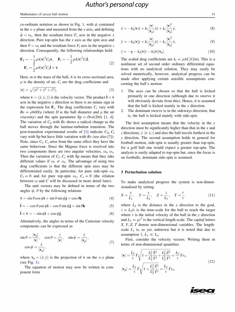
co-ordinate notation as shown in Fig. 1, with w contained

in the x–y plane and measured from the x axis, and defining_w ¼ xs; then the resultant force Fs acts in the negative x

direction. Pure top-spin has the x axis as the spin axis and

then _h ¼ xl and the resultant force Fl acts in the negative z

direction. Consequently, the following relationships hold:

Fd ¼ �1

2qAjvj2Cdv; Fl ¼ �

1

2qAjvj2Cll;

Fs ¼1

2qAjvj2Csl� v:

ð2Þ

Here, m is the mass of the ball, A is its cross-sectional area,

q is the density of air, Ci are the drag coefficients and

jvj ¼ffiffiffiffiffiffiffiffiffiffiffiffiffiffiffiffiffiffiffiffiffiffiffiffiffiffiffiffi

ð _x2 þ _y2 þ _z2Þp

; ð3Þ

where v ¼ ð _x; _y; _zÞ is the velocity vector. The product l� v

acts in the negative x direction so there is no minus sign in

the expression for Fs. The drag coefficients Ci vary with

Re = q|v|D/l (where D is the ball diameter and l the air

viscosity) and the spin parameter Sp = Dx/(2|v|) [1, 4].

The variation of Cd with Re shows a radical change as the

ball moves through the laminar-turbulent transition. The

post-transition experimental results of [1] indicate Cd, Cl

vary with Sp but have little variation with Re (see also [7]).

Note, since Cl, Cs arise from the same effect they have the

same behaviour. Since the Magnus force is resolved into

two components there are two angular velocities, xl, xs.

Then the variation of Cl, Cs with Sp means that they take

different values if xl = xs. The advantage of using two

drag coefficients is that the different spin axes may be

differentiated easily. In particular, for pure side-spin xl,

Cl = 0 and for pure top-spin xs, Cs = 0 (the relation

between x and C will be discussed in more detail later).

The unit vectors may be defined in terms of the two

angles w, h by the following relations

v ¼ sin h cos wiþ sin h sin wjþ cos hk ð4Þ

l ¼ � cos h cos wi� cos h sin wjþ sin hk ð5Þ

l� v ¼ � sin wiþ cos wj: ð6Þ

Alternatively, the angles in terms of the Cartesian velocity

components can be expressed as

sin h ¼ jvpjjvj ; cos h ¼ _z

jvj ; sin w ¼ _y

jvpj;

cos w ¼ _x

jvpj;

ð7Þ

where vp ¼ ð _x; _yÞ is the projection of v on the x–y plane

(see Fig. 1).

The equation of motion may now be written in com-

ponent form

€x ¼ �kdjvj _xþ kl

jvjjvpj

_x _zþ ks

jvj2

jvpj_y; ð8Þ

€y ¼ �kdjvj _yþ kl

jvjjvpj

_y _z� ks

jvj2

jvpj_x; ð9Þ

€z ¼ �g� kdjvj _z� kljvjjvpj: ð10Þ

The scaled drag coefficients are ki = qACi/(2m). This is a

nonlinear set of second order ordinary differential equa-

tions with no analytical solution. They may easily be

solved numerically, however, analytical progress can be

made after applying certain sensible assumptions con-

cerning the ball’s motion:

1. The axes can be chosen so that the ball is kicked

primarily in one direction (although due to swerve it

will obviously deviate from this). Hence, it is assumed

that the ball is kicked mainly in the y direction.

2. The dominant swerve is in the sideways direction, that

is, the ball is kicked mainly with side-spin.

The first assumption means that the velocity in the y

direction must be significantly higher than that in the x and

z directions, _y� _x; _z and also the ball travels furthest in the

y direction. The second assumption holds in general for

football motion, side-spin is usually greater than top-spin,

for a golf ball one would expect a greater top-spin. The

analysis is easily adapted to top-spin but, since the focus is

on footballs, dominant side-spin is assumed.

3 Perturbation solution

To make analytical progress the system is non-dimen-

sionalised by setting

X ¼ x

L1

; Y ¼ y

L2

; Z ¼ z

L3

; T ¼ t

s: ð11Þ

where L2 is the distance in the y direction to the goal,

s = L2/v is the time-scale for the ball to reach the target

where v is the initial velocity of the ball in the y direction

and L3 = gs2 is the vertical length-scale. The capital letters

X, Y, Z, T denote non-dimensional variables. The length-

scale L1 is, as yet, unknown but it is noted that due to

assumption 1, L1 � L2.

First, consider the velocity vectors. Writing them in

terms of non-dimensional quantities

jvj ¼ L2

s_Y

ffiffiffiffiffiffiffiffiffiffiffiffiffiffiffiffiffiffiffiffiffiffiffiffiffiffiffiffiffiffiffiffiffiffiffi

1þ L21

L22

_X2

_Y2þ L2

3

L22

_Z2

_Y2

s

¼ L2

s_Yr1;

jvpj ¼L2

s_Y

ffiffiffiffiffiffiffiffiffiffiffiffiffiffiffiffiffiffiffi

1þ L21

L22

_X2

_Y2

s

¼ L2

s_Yr2;

ð12Þ

Mathematics of soccer ball motion 31

Author's personal copy

where r1, r2 denote the square roots. The factor L2_Y=s has

been isolated since this is the largest term in the velocity

expression and so r1; r2 ¼ Oð1Þ (i.e. their size is of the

order unity).

The governing equations may now be written as:

€X ¼ �kdL2_X _Yr1 þ klL3

r1

r2

_X _Z þ ks

L22r2

1

L1r2

_Y2 ð13Þ

€Y ¼ �kdL2_Y2r1 þ klL3

r1

r2

_Y _Z � ks

L1r21

r2

_X _Y ð14Þ

€Z ¼ �1� kdL2r1_Y _Z � kl

L22

L3

r1r2_Y2 ð15Þ

To determine L1, it is noted that the motion in the x

direction is caused by either an initial velocity or the spin

component in the y direction. Since this study is focussed

on the spin-induced swerve, the initial velocity in the x

direction is set to zero, _xð0Þ ¼ _Xð0Þ ¼ 0: The dominant

term in Eq. (13) is clearly that involving _Y2 and since the

velocity vectors are scaled so that r1; r2 ¼ Oð1Þ; L1 ¼ ksL22:

Using the parameter values of Table 1 this determines L1

& 4 m, that is, the ball is expected to travel in the of order

4 m laterally during its flight. The dominant term in

Eq. (14) again involves _Y2: With kd = 0.013, kdL2 = 0.26

and this is denoted as � ¼ kdL2 which is a small parameter

(and �2 � 0:07). The square root terms r1, r2 contain the

ratios L12/L2

2 & 0.04, L32/L2

2 & 0.25 which are denoted

c1�2; c2�, respectively (note, ksL1 = L1

2/L22). Finally,

klL3 � 0:03 ¼ c3�2; klL

22=L3 � 0:27 ¼ c4�:

The governing equations are now

€X ¼ � _Yr1 � _X � c3�2

_X _Z

r2_Y� r1

r2

_Y

� �

ð16Þ

€Y ¼ � _Yr1 � _Y � c3�2

_Z

r2

þ c1�2 r1

r2

_X

� �

ð17Þ

€Z ¼ �1� _Yr1½� _Z þ c4�r2_Y � ð18Þ

where

r1 ¼

ffiffiffiffiffiffiffiffiffiffiffiffiffiffiffiffiffiffiffiffiffiffiffiffiffiffiffiffiffiffiffiffiffiffiffiffiffiffiffiffi

1þ c1�2_X2

_Y2þ c2�

_Z2

_Y2

s

; r2 ¼

ffiffiffiffiffiffiffiffiffiffiffiffiffiffiffiffiffiffiffiffiffiffi

1þ c1�2_X2

_Y2

s

: ð19Þ

Note the assumption that the ball is kicked primarily with

side-spin means that the kl terms enter at lower order to the

ks terms in the €X; €Y equations (through the coefficient c3).

In the €Z equation lift is the dominant force after gravity and

so it enters at Oð�Þ: With top-spin dominating the scaling

would have to be changed accordingly.

Written in non-dimensional form observations can be

made about the solution behaviour, without solving the

system. For example, all terms in (17) involve the small

parameter � indicating that the dominant motion in the Y

direction is described by €Y ¼ 0 and that drag, represented

by �; has a relatively small effect. Since � ¼ 0:26

neglecting terms involving � could lead to errors of around

26 %. Motion in the Z direction is dominated by gravity.

The X motion is dominated by the contribution of _Y

(reflecting the fact that the Magnus force is due to the

difference in equatorial velocities and the forward velocity,

which is approximately _Y). However, the most interesting

feature is that since r1 contains the term �ð _Z= _YÞ2 the

velocity in the Z direction will contribute to all equations.

Most importantly, it will affect the X equation at order �;

i.e. for the current set of parameter values neglect of the Z

motion may lead to errors of around 26 %. Obviously, this

could have significant consequences for any experiment

using a two-dimensional analysis to model the three-

dimensional ball motion. This is discussed further in

Sect. 4.

The initial conditions are that the ball starts at the origin

and is kicked with (dimensional) velocity (0, v, w). Note,

the velocity in the x direction could always be chosen to be

zero by simply defining the y axis as the direction of the

kick in the x–y plane. In non-dimensional form these

conditions are Xð0Þ ¼ Yð0Þ ¼ Zð0Þ ¼ 0; _Xð0Þ ¼ 0; _Yð0Þ ¼1; _Zð0Þ ¼ W ; where W = ws/L3.

In order to determine a standard perturbation solution

based on the small parameter � write

X ¼ X0 þ �X1 þ �2X2 þ � � � ; Y ¼ Y0 þ �Y1 þ �2Y2 þ � � � ;Z ¼ Z0 þ �Z1 þ �2Z2 þ � � �

ð20Þ

To Oð�2Þ the solution is

X ¼ T2

2þ � c2W2T2

2� ð3þ 2c2WÞ T

3

6þ c2T4

12

� �

þ �2 � 9

2c2W2 þ 3c3W � 2c2c4W

� �

T3

6

�

þ 6c2W þ 11

2� 2c3 �

c1

2þ 2c2c4

� �

T4

12� 13c2T5

120

�

ð21Þ

Table 1 Typical parameter values (see [1, 5, 15])

kd 0.013 kl 0.004

ks 0. 0108 m 0.45 kg

q 1 kg/m3 D 0.22 m

A 0.039 m2 v 25 m/s

Cd 0.3 Cs 0.25

Cl 0.1 L2 20 m

32 T. G. Myers, S. L. Mitchell

Author's personal copy

Y ¼ T � � T2

2þ �2

� �ðc2W2 � 2c3WÞ T2

4þ ð2� c1 þ c2W � c3Þ

T3

6� c2T4

24

� �

ð22Þ

Z ¼ WT � T2

2þ � �ðW þ c4Þ

T2

2þ T3

6

� �

þ �2 �c2W2ðW þ c4ÞT2

4þ ð4W þ 6c4 þ 3c2W2

�

þ 2c2c4WÞ T3

12� ð3þ 3c2W þ c2c4Þ

T4

24þ c2T5

40

�

:

ð23Þ

Bray and Kerwin’s [3] study a simplified two-

dimensional system. This analysis follows the line of

equating the acceleration to the largest term on the right

hand side of the equations. From Eqs. (16, 17) this reduces

the problem to

€X ¼ _Y2; €Y ¼ �� _Y2; ð24Þ

where it is noted that r1 & r2 & 1. Applying the initial

conditions gives

Y ¼ 1

�ln j1þ �T j; X ¼ � 1

�ðY � TÞ: ð25Þ

To relate these solutions to Eqs. (21, 22), the Taylor series

expansion for �� 1 is used to find

X ¼ T2

2� � T3

3þ �2 T4

4ð26Þ

Y ¼ T � � T2

2þ �2 T3

3: ð27Þ

Setting W, ci = 0 in (21, 22), to remove the Z dependence

and make the solution appear two-dimensional, the x

solutions differ at Oð�Þ; while the y solutions differ at

Oð�2Þ: The simplification of only taking the largest terms

on the right hand side will therefore correctly capture the

dominant behaviour but, in the case of the sideways

swerve, leads to errors in all subsequent terms. Conse-

quently, this solution form will provide a reasonable

approximation to the numerical result for y, but a rather

poorer one for x and the error increases with � (e.g. if L2 is

increased). Further deviation from the correct solution will

occur due to the neglect of the Z motion. This will be

discussed later in the context of the solutions shown in

Sect. 4.

Now return to dimensional variables X = x/L1, Y = y/

L2, Z = z/L3, T = t/s, where L1 = ksL22, L3 = gs2, s = L2/v

and L2, v are the initial distance and velocity in the y

direction. The constants must also be expressed in terms of

the dimensional parameters

� ¼ kdL2; c1 ¼k2

s

k2d

; c2 ¼g2L2

kdv4; c3 ¼

klg

vk2dL2

;

c4 ¼klv

2

gkdL2

; W ¼ wv

gL2

:

ð28Þ

The dimensional solution is then given by

x ¼ ksðvtÞ2

21� kdvt � g2t2 � 4gwt þ 6w2

6v2

� �� �

ð29Þ

y ¼ vt 1� kdvt

2

� �� �

ð30Þ

z ¼ wt � gt2

2þ kdgvt3

6� kdwþ klvð Þ vt2

2

� �

: ð31Þ

Note, since the expressions are rather cumbersome they are

only written here to Oð�Þ (the Oð�Þ terms are given in the

curly brackets). From these expressions the effect of the

various parameters can be seen clearly. The y equation

shows that the distance travelled is approximately propor-

tional to the initial velocity and time but that drag reduces

this and the effect of drag increases with time. In the z

direction the distance travelled is determined primarily by

the initial velocity and gravity but both drag and lift act to

change this. Again these effects increase with time. How-

ever, since swerve due to side-spin is the main focus of this

study the x equation is the most revealing. From this it is

seen that, to leading order the distance travelled in the x

direction is proportional to the sideways drag coefficient ks

and also (vt)2. The ball design and atmospheric conditions

contribute through ks; hence, ball design is very important

for swerve. The product vt is the first approximation to the

distance travelled in the y direction. The quadratic depen-

dence then indicates the importance of taking a kick far

from the goal. The further the ball travels the more it will

swerve (this is obviously well known to free kick spe-

cialists in football who frequently attempt to move the ball

away from the goal). Perhaps, the most famous example is

the free kick of Roberto Carlos against France in 1997

which exhibited spectacular curve at the end of the flight.

This free kick was taken approximately 35 m from goal,

see YouTube or [6]. The forward drag kd enters at first

order and acts to reduce the swerve. An important feature

of the solution is that the vertical motion, through g and

w, also enters at first order. The quadratic g2t2 - 4gwt ?

6w2 is positive provided w C 0 (i.e. the ball is not kicked

into the ground) and so acts to increase the swerve.

A two-dimensional analysis will miss this effect and

comparison with experiment would then lead to over-

prediction of ks.

Due to the differences in time dependence of the terms

in Eqs. (29–31) they will become less accurate as time

increases. This is termed the secular effect. The break

Mathematics of soccer ball motion 33

Author's personal copy

down will occur when the Oð�Þ terms become Oð1Þ: In the

case of the x equation this is when t * 1/(kdv) & 3 s. The

y and z equations indicate times around 9 s. Given that the

football flight is typically 1 s these approximations should

hold for all sensible kicks and the secular effect is not

considered.

4 Numerical and analytical results

The numerical solution to Eqs. (16–18) was carried out

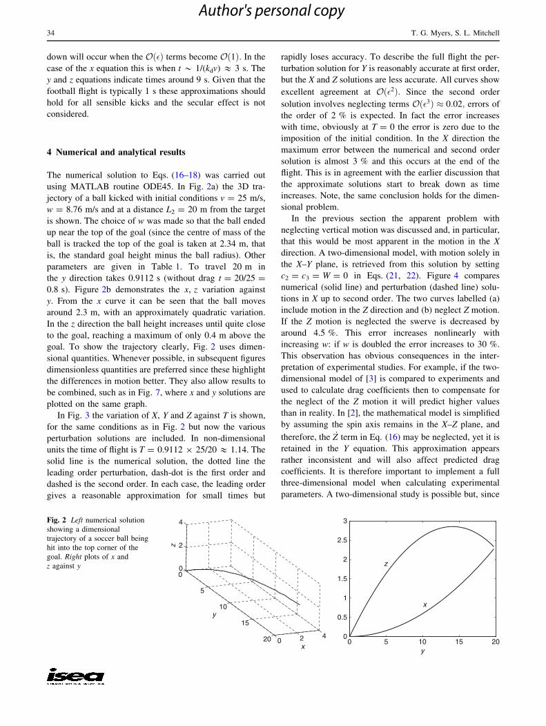
using MATLAB routine ODE45. In Fig. 2a) the 3D tra-

jectory of a ball kicked with initial conditions v = 25 m/s,

w = 8.76 m/s and at a distance L2 = 20 m from the target

is shown. The choice of w was made so that the ball ended

up near the top of the goal (since the centre of mass of the

ball is tracked the top of the goal is taken at 2.34 m, that

is, the standard goal height minus the ball radius). Other

parameters are given in Table 1. To travel 20 m in

the y direction takes 0.9112 s (without drag t = 20/25 =

0.8 s). Figure 2b demonstrates the x, z variation against

y. From the x curve it can be seen that the ball moves

around 2.3 m, with an approximately quadratic variation.

In the z direction the ball height increases until quite close

to the goal, reaching a maximum of only 0.4 m above the

goal. To show the trajectory clearly, Fig. 2 uses dimen-

sional quantities. Whenever possible, in subsequent figures

dimensionless quantities are preferred since these highlight

the differences in motion better. They also allow results to

be combined, such as in Fig. 7, where x and y solutions are

plotted on the same graph.

In Fig. 3 the variation of X, Y and Z against T is shown,

for the same conditions as in Fig. 2 but now the various

perturbation solutions are included. In non-dimensional

units the time of flight is T = 0.9112 9 25/20 & 1.14. The

solid line is the numerical solution, the dotted line the

leading order perturbation, dash-dot is the first order and

dashed is the second order. In each case, the leading order

gives a reasonable approximation for small times but

rapidly loses accuracy. To describe the full flight the per-

turbation solution for Y is reasonably accurate at first order,

but the X and Z solutions are less accurate. All curves show

excellent agreement at Oð�2Þ: Since the second order

solution involves neglecting terms Oð�3Þ � 0:02; errors of

the order of 2 % is expected. In fact the error increases

with time, obviously at T = 0 the error is zero due to the

imposition of the initial condition. In the X direction the

maximum error between the numerical and second order

solution is almost 3 % and this occurs at the end of the

flight. This is in agreement with the earlier discussion that

the approximate solutions start to break down as time

increases. Note, the same conclusion holds for the dimen-

sional problem.

In the previous section the apparent problem with

neglecting vertical motion was discussed and, in particular,

that this would be most apparent in the motion in the X

direction. A two-dimensional model, with motion solely in

the X–Y plane, is retrieved from this solution by setting

c2 = c3 = W = 0 in Eqs. (21, 22). Figure 4 compares

numerical (solid line) and perturbation (dashed line) solu-

tions in X up to second order. The two curves labelled (a)

include motion in the Z direction and (b) neglect Z motion.

If the Z motion is neglected the swerve is decreased by

around 4.5 %. This error increases nonlinearly with

increasing w: if w is doubled the error increases to 30 %.

This observation has obvious consequences in the inter-

pretation of experimental studies. For example, if the two-

dimensional model of [3] is compared to experiments and

used to calculate drag coefficients then to compensate for

the neglect of the Z motion it will predict higher values

than in reality. In [2], the mathematical model is simplified

by assuming the spin axis remains in the X–Z plane, and

therefore, the _Z term in Eq. (16) may be neglected, yet it is

retained in the Y equation. This approximation appears

rather inconsistent and will also affect predicted drag

coefficients. It is therefore important to implement a full

three-dimensional model when calculating experimental

parameters. A two-dimensional study is possible but, since

0

5

10

15

20 0 2 4

0

2

4

x

y

z

0 5 10 15 200

0.5

1

1.5

2

2.5

3

y

z

x

Fig. 2 Left numerical solution

showing a dimensional

trajectory of a soccer ball being

hit into the top corner of the

goal. Right plots of x and

z against y

34 T. G. Myers, S. L. Mitchell

Author's personal copy

gravity cannot be avoided, this should be confined to the Y–

Z plane and using only top-spin.

4.1 Comparison with experimental data

In the paper of Carre et al. [5] a number of results are

presented for ball motion with and without spin. In their

Figures 4a–c, a typical trajectory is shown for a ball

launched with no spin at approximately 15� to the ground

and with a launch velocity in the range of 17–31 m/s.

Taking the data from these figures, it is a simple matter to

fit a curve (in this case the polyfit function in Matlab was

used, which fits data using a least-squares criteria). A

quadratic fit to the y(t) data of their Figure 4b leads to

y � a0 þ a1t þ a2t2; ð32Þ

where a0 = -0.1785, a1 = 17.591, a2 = -1.237. A cubic

fit to the z(t) data of Figure 4c leads to

z � b0 þ b1t þ b2t2 þ b3t3; ð33Þ

where b0 = 0.0253, b1 = 6.287, b2 = -6.294, b3 = 0.201.

The appropriate data points are displayed in Fig. 5 as

asterisks. Finally, Fig. 4a presents z(y) which takes the

form

z � c0 þ c1yþ c2y2 þ c3y3; ð34Þ

where c0 = 0.008, c1 = 0.371, c2 = -0.023, c3 = 0.0001.

From these relations it is a simple matter to determine a

number of the flight parameters. For example, the initial

angle of the kick, h, is determined by noting

tan h ¼ _zð0Þ_yð0Þ ¼

b1

a1

� 6:287

17:591� 0:357: ð35Þ

Alternatively, tan h ¼ dz=dyjy¼0 ¼ c1 � 0:371: These two

results indicate a launch angle of h & 19.65 or 20.35, with

an average of approximately 20� (slightly higher than that

quoted in the paper). The initial velocity in the y, z direc-

tions is ð _yð0Þ; _zð0ÞÞ ¼ ða1; b1Þ ¼ ð17:591; 6:287Þ and so the

initial speed jvj ¼ffiffiffiffiffiffiffiffiffiffiffiffiffiffiffi

a21 þ b2

1

p

� 18:68 m/s, which is within

the quoted range.

0 0.2 0.4 0.6 0.8 1 1.20

0.5

X

0 0.2 0.4 0.6 0.8 1 1.20

0.5

1

Y

0 0.2 0.4 0.6 0.8 1 1.20

0.5

T

Z

Fig. 3 Non-dimensional trajectories of X, Y and Z against T: full

numerical solution (solid line), Oð�0Þ solution (dotted line), Oð�Þsolution (dot-dashed line) andOð�2Þ solution (dashed line). Parameter

values are Cd = 0.3, Cs = 0.25 and Cl = 0.1

0 0.2 0.4 0.6 0.8 10

0.1

0.2

0.3

0.4

0.5

T

X

(a)

(b)

Fig. 4 Comparison of numerical (solid line) and second order

perturbation (dashed line) solutions in X: a including vertical motion,

b neglecting vertical motion

0 0.1 0.2 0.3 0.4 0.5 0.60

2

4

6

8

10y (m)

t (s)

0 0.1 0.2 0.3 0.4 0.5 0.60

0.2

0.4

0.6

0.8

1

1.2

1.4

1.6

z (m)

t (s)

Fig. 5 Comparison of experimental data of [5] (asterisks) and curve

fits (solid line)

Mathematics of soccer ball motion 35

Author's personal copy

Comparison of the curve fit equations (32, 33) and the

perturbation solutions (30, 31) allows us to determine

additional information about the kick. First, it may be noted

that both y, z should start at the origin, which is the case

with the perturbation solution, but the curve fit indicates

some slight error. However, both the relevant terms b0, c0

are small. The values for (v, w) are obtained from taking

ð _yð0Þ; _zð0ÞÞ in Eqs. (30, 31) and obviously (v, w) =

(a1, b1). The drag coefficient kd may be obtained by com-

paring the quadratic terms in the y expressions

� kdv2

2¼ a2 ) kd ¼ 0:008; ð36Þ

which is of a similar order of magnitude to that quoted in

Table 1. The z expressions provide a means for verifying

this value, comparing the cubic terms gives

kdgv

6¼ b3 ) kd ¼ 0:007; ð37Þ

which, allowing for experimental error and errors in curve

fitting, appears to be in good agreement with the first

estimate. In [5] it is stated that this trajectory is typical for a

case with no spin, consequently kl = 0. There is then a

third way to determine kd: comparison of the quadratic

terms in the z expressions. This leads to kd & 0.025, a

result that is clearly at odds with the previous findings.

However, allowing kl = 0 the quadratic terms may be

used to determine kl = 0.0061 when kd = 0.008 and

kl = 0.0065 when kd = 0.007.

In Fig. 5a the experimental data is compared against the

quadratic form given by Eq. (32) with the quoted values for

ai. This is equivalent to plotting the approximate solution

(30) with v = 17.591 m/s, kd = 0.008. Clearly, the agree-

ment is excellent. In Fig. 5b the experimental data is

compared against the cubic form given by Eq. 33 with the

quoted values for bi. This is equivalent to plotting the

approximate solution (31) with w = 6.287 m/s, kd = 0.007.

Again the agreement is excellent.

In summary, the forms suggested by the perturbation

solution can provide an excellent fit to the experimental

data. Comparison between the coefficients of the fitted

curve and the perturbation solutions then permits the cal-

culation of the drag coefficients (and can also be used to

determine initial velocities if these are unknown). As an

example, the data provided in [5] was used to determine

flight parameters, indicating an initial angle of around 20�(as opposed to the reported 15�), a drag coefficient kd 2½0:007; 0:008� and a lift coefficient kl 2 ½0:0061; 0:0065�:The appearance of a non-zero lift coefficient for an

experiment apparently with no spin is particularly inter-

esting. Given that the equations provide three ways to

calculate kd in the absence of spin, and that two of these

routes agree well, it seems likely that the fault does not lie

in the equations. Consequently, we may infer that possibly

the graphs have been misreported (they are in fact only

presented as a ‘typical’ solution) or that some spin was

generated during the flight, perhaps due to the initial

position of the seams or the valve.

5 Drag coefficients

So far, the analysis has dealt with constant drag coefficients.

However, experimental studies have shown that Cd, Cl, Cs all

vary with spin rate Sp = Rx/|v| and, to a lesser extent (pro-

vided the air flow is turbulent), the Reynolds number. During

the flight of a ball the angular velocity decays very slowly

[11]. This may also be observed in the experimental findings

of [9] and so angular velocity may reasonably be taken as

constant, but the magnitude of |v| decreases due to the drag

and so Sp increases.

There exist numerous experimental studies showing the

variation of Cs (or Cl) with Sp (see [1, 4, 9, 14] for example).

Goff and Carre [7] summarise experimental results of Asai

et al. [1] and Carre et al. [4]. They point out that since Cl and

Cs arise from the same process they are equivalent (some

authors do not split the lift coefficient into components,

preferring to work with a single one defined on an appropriate

spin axis, see [11] for example). The experimental results

indicate that Cs, Cl increase with spin until levelling off

around Sp = 0.3. The actual values vary between experi-

ments and, as shown in [14], with different types of ball but

typically range between 0 and 0.35 as Sp increases from 0 to

0.3 [1, 5, 9, 15]. Since the focus of this study is on the effect of

spin in these calculations the region where Sp is very small

(below 0.1) is neglected and then a piecewise approximation

is employed of the form

Cs ¼Cs0 1þ ms

Cs0ðSp� Sp0Þ

; 0:1\Sp\0:3

Cs0 1þ ms

Cs0ð0:3� Sp0Þ

¼ Csm; Sp [ 0:3;

8

<

:

ð38Þ

where the gradient ms = 0.8, Cs0 = 0.25 is the coefficient

when Sp = Sp0 = 0.15/0.8 and Csm = 0.34 is the constant

maximum value of Cs. The drag coefficient ks = ks0 is now

written

ks0 ¼qACs0

2m:

The linear form, without the cut-off, has also been

employed by Horzer et al. [11]. The drag coefficient Cd

shows a weaker dependence on Sp and so as a first attempt

to model varying coefficients Cs is allowed to vary and Cd

is left constant.

Given the equivalence of Cs, Cl, only the effect of

varying one of these quantities is studied. This is fortunate

36 T. G. Myers, S. L. Mitchell

Author's personal copy

since, as pointed out in the previous section, the analysis

should be three-dimensional (unless limited to the y–z

plane with only top-spin imposed). If both Cs and Cl are

allowed to vary then the perturbation will be extremely

cumbersome. Instead the case of pure side-spin is studied

by setting Cl = kl = 0 while Cs is given by Eq. (38). The

non-dimensional model then reduces to

€X ¼ � _Yr1 kdL2_X � ks0/s

L22r1

L1r2

_Y

� �

ð39Þ

€Y ¼ � _Yr1 kdL2_Y þ ks0/s

L1r1

r2

_X

� �

ð40Þ

€Z ¼ �1� kdL2r1_Y _Z: ð41Þ

where

/s ¼1þ ms

Cs0ðSp� Sp0Þ; 0:1\Sp\0:3

Csm

Cs0; Sp [ 0:3;

(

ð42Þ

and

Sp ¼ Dx2jvj ¼

Dx

2r1v _Y: ð43Þ

Defining

/s ¼/1

r1_Yþ /2; /1 ¼

msRxCs0v

; /2 ¼ 1� msSp0

Cs0

: ð44Þ

To retrieve the constant spin case the conditions set were

/1 = 0, /2 = 1. Retaining the previous definitions for the

small parameters (but with ks replaced by ks0) the

governing equations may be written as

€X ¼ � _Yr1 � _X � /1

r1_Yþ /2

� �

r1

r2

_Y

� �

ð45Þ

€Y ¼ � _Yr1 � _Y þ c1�2 /1

r1_Yþ /2

� �

r1

r2

_X

� �

ð46Þ

€Z ¼ �1� �r1_Y _Z: ð47Þ

The variable spin is represented through the term involving

/1 and this appears at leading order in the €X equation.

Hence, variable spin is expected to have a significant effect

on the X motion. However, /1 and X only appear in the €Y

and €Z equations at second order and so it is expected that

variable spin has little effect on the Y, Z motion.

Using a standard perturbation, to Oð�Þ the solutions are

X ¼ ð/1 þ /2ÞT2

2

þ � c2W2ð/1 þ 2/2ÞT2

4��

/1ð2þ c2WÞ�

þ /2ð3þ 2c2WÞ� T3

6þ c2ð/1 þ 2/2ÞT4

24

�

ð48Þ

Y ¼ T � � T2

2; Z ¼ WT � T2

2þ � �WT2

2þ T3

6

� �

ð49Þ

Noting that kl = 0 leads to c3 = c4 = 0 and then the Y and

Z solutions above correspond to Eqs. (21–23) to Oð�Þwhile the X solution differs from Eq. (21) at leading order.

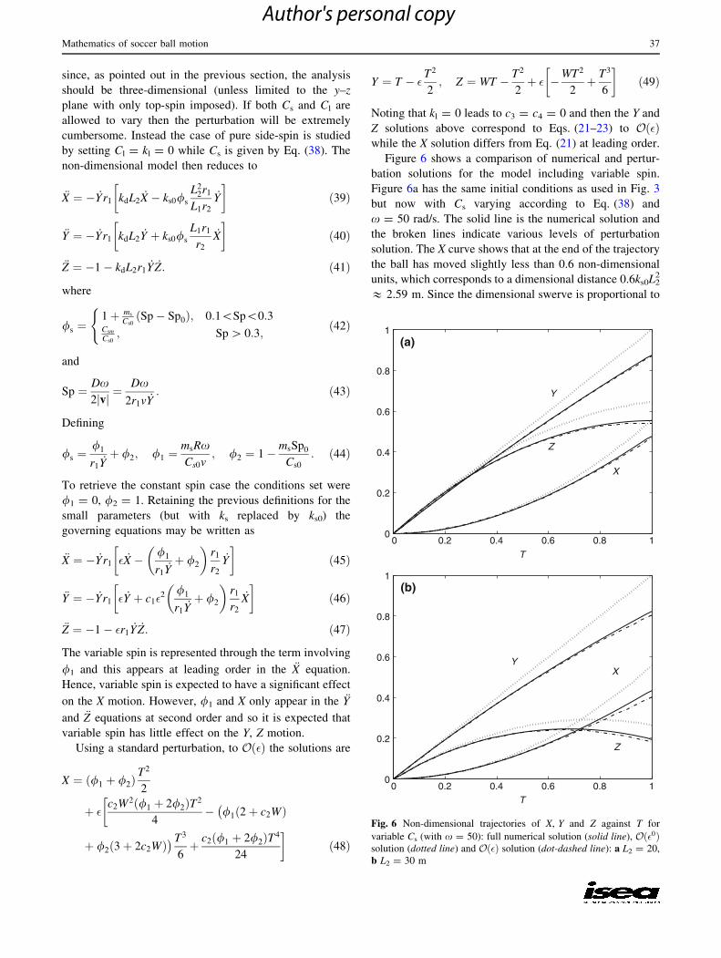
Figure 6 shows a comparison of numerical and pertur-

bation solutions for the model including variable spin.

Figure 6a has the same initial conditions as used in Fig. 3

but now with Cs varying according to Eq. (38) and

x = 50 rad/s. The solid line is the numerical solution and

the broken lines indicate various levels of perturbation

solution. The X curve shows that at the end of the trajectory

the ball has moved slightly less than 0.6 non-dimensional

units, which corresponds to a dimensional distance 0.6ks0L22

& 2.59 m. Since the dimensional swerve is proportional to

0 0.2 0.4 0.6 0.8 10

0.2

0.4

0.6

0.8

1

T

Y

Z

X

(a)

0 0.2 0.4 0.6 0.8 10

0.2

0.4

0.6

0.8

1

T

YX

Z

(b)

Fig. 6 Non-dimensional trajectories of X, Y and Z against T for

variable Cs (with x = 50): full numerical solution (solid line), Oð�0Þsolution (dotted line) and Oð�Þ solution (dot-dashed line): a L2 = 20,

b L2 = 30 m

Mathematics of soccer ball motion 37

Author's personal copy

L2, in Fig. 6b the same kick is shown but now taken from

30 m away. The change in L2 results in an increase in

� ¼ kdL2 and so it is expected that the perturbation solution

will lose accuracy. This is clear from the figure, however,

the Oð�Þ solution is still relatively accurate (accuracy could

be increased by finding the Oð�2Þ term). The dimensional

swerve at the end of the kick is now around 4.86 m. This is

almost double that of the 20 m kick and results from the

approximately quadratic dependence on distance.

In Fig. 7a four curves corresponding to x = 30,

40, 50, 60 rad/s and L2 = 30 m are plotted (with other

conditions as in Fig. 3). As expected, increasing xincreases the lateral motion such that X(1) ranges from

0.298 to 0.44 as x increases from 30 to 60 (and dimen-

sionally from 2.9m to 4.3 m). Neglecting variable drag,

Eq. (29) indicates that the increase should be approxi-

mately linear x � ks. Including the variation in drag coef-

ficient, with a cut-off, makes the increase nonlinear. For

example, as x increases from 30 to 40 X(1) increases by

0.052 (dimensionally 0.5 m), but as increasing x from 50

to 60 X(1) increases by only 0.04 (dimensionally 0.4 m).

Increasing x further will make very little difference to the

motion. This may be understood through Fig. 7b which

shows the variation of Cs through the trajectory: with

x = 30 or 40 the value of Cs is always increasing. When

x = 50 the value of Cs becomes constant near the end of

the flight and for x = 60 it is constant half of the time.

Consequently, any kick with x[ 60 will provide a similar

result as that with x = 60.

In carrying out this study the question arose as to what

exactly is being presented by different research groups

when plotting Cs - Sp curves. In particular, it appears

unclear how Sp = Rx/|v| is interpreted. The experiments

of Asai et al. [1] and Passmore et al. [15] involve a ball

fixed in a wind tunnel where both x and v remain constant

and so Sp takes a single value for each experiment. The

drag and lateral force are measured directly, which then

allows calculation of drag coefficients through the defini-

tions of Eq. (2). More ‘realistic experiments’ involve

actually kicking the ball in a controlled environment and

then calculating coefficients by matching the data to some

mathematical model. For example, Bray and Kerwin [2]

track a ball’s flight with two cameras. The model equations

are solved and iterated, using the drag coefficients as fitting

parameters, until a good fit to the experimental data is

achieved. By this method constant values for forward and

lateral drag coefficients are determined for a given kick.

However, since these values come from fitting to the full

trajectory, where Sp is an increasing function, the coeffi-

cients must be some form of average for the specific kick.

A similar technique is employed by Carre et al. [5] where

drag coefficients are also averages, but plots are against the

initial value of Sp (thus avoiding the confusion in the

variation of Sp). Goff and Carre [7, 8] fit drag coefficients

to minimise the least-squares error between a numerical

solution and experimental data, but to reduce variation in

Sp they limit data to the first 0.07s of flight. Griffiths et al.

[9] use an accurate ball tracking method but then calculate

coefficients using the formula of Wesson [16] which

assumes constant drag. Consequently, the various data

presented may show actual Cs and Sp values or may be

average values over a given trajectory (with different

methods of averaging). Figure 8 presents two sets of

curves; the bottom curves correspond to variable Cs with

L2 = 30 m. The dashed line represents the ball trajectory

up to t = 1.655 s (to end at y & 30 m), the solid line ends

at t = 0.693 s (around y = 15 m). The top curves use a

constant value of Cs = 0.307 which was chosen to match

the variable Cs result after 1.655 s. The graph is presented

dimensionally, since the non-dimensional scaling depends

on the choice of Cs. All other conditions are the same as in

0 0.2 0.4 0.6 0.8 10

0.05

0.1

0.15

0.2

0.25

0.3

0.35

0.4

0.45

T

X

ωs = 60

ωs = 50

ωs = 40

ωs = 30

0.1 0.2 0.3 0.4

0.2

0.25

0.3

0.35

Sp

Cs

0.1 0.2 0.3 0.4

0.2

0.25

0.3

0.35

Sp

Cs

0.1 0.2 0.3 0.4

0.2

0.25

0.3

0.35

Sp

Cs

0.1 0.2 0.3 0.4

0.2

0.25

0.3

0.35

Sp

Cs

ωs = 30 ω

s = 40

ωs = 50 ω

s = 60

Fig. 7 a Non-dimensional trajectories of x against t for variable

Cs, b corresponding plots of Cs against Sp, dashed line represents

Eq. (38) the thick solid line is the variation of Cs over the trajectory

38 T. G. Myers, S. L. Mitchell

Author's personal copy

the x = 50 rad/s case of Fig. 7. The important feature here

is that for times not equal to 1.655 s the constant Cs curve

has a different amount of swerve which indicates that if an

average value is used for Cs then its value will vary with

the distance of the kick (in the figure the 15 m kicks show a

difference of 10cm in swerve). That is, if all other condi-

tions are fixed fitting a constant Cs value to experimental

data will lead to range of Cs values for kicks taken over

different distances.

6 Discussion

In this study, the three-dimensional equations of motion for

a football in flight have been studied. The numerical

solution is trivial but this does not show the dependence on

the problem parameters. Consequently, a perturbation

solution was developed which proved highly accurate when

compared to the numerical solution. In deriving this solu-

tion the scaling was based on the assumption that foot-

ballers impart more lateral than top-spin. This could easily

be changed, to study a golf ball for example, where top-

spin dominates. The analysis allowed a number of obser-

vations to be made about the ball’s motion.

The analytical approximations show that at leading

order the lateral motion is proportional to the lateral drag

coefficient ks and the distance (vt)2. This indicates why free

kicks taken from a large distance show greater swerve. To

first order in the small parameter, the motion in each

direction is at most described by a quartic equation in time.

Experimental studies often approximate data with a poly-

nomial. For example, Carre et al. [5] show excellent

agreement with data assuming x varies quadratically in t.

This is in agreement with this study’s leading order result x

& ks (vt)2/2 and so will capture the dominant behaviour

and small time solution well. Bray and Kerwin [2] assume

a quartic dependence for x, y, z: since a quartic contains

more coefficients it can more accurately fit the data. This

form agrees with the first order expression. For this reason

the results presented here were not initially compared with

experimental data: numerous studies have shown that the

data may be well approximated by quadratic or quartic

functions. Since the results take this form, equally good

agreement can be obtained by simply choosing appropriate

coefficients (and so inferring values for the drag coeffi-

cients). However, at the insistence of a referee the results

were compared to those given in [5], showing the expected

excellent agreement and allowing for easy determination of

flight parameters. In fact, this shows that in a sense the

governing equations may be considered as rather forgiving

in that an inaccurate model will still allow good agreement

with experimental data. Missing out terms, for example by

studying only the two-dimensional motion, will lead to the

same form of solution as the three-dimensional system but

the polynomial coefficients will be different. As a conse-

quence, a numerical study of a slightly incorrect set of

governing equations will be able to provide excellent

agreement with experimental data but the drag coefficients

calculated from this solution will differ from the true val-

ues. To illustrate this, Eqs. (29, 30) are combined to

determine an expression for x as a function of y, accurate to

Oð�Þ;

x ¼ ksy2

21þ w2

v2� 2gwy

3v3þ g2y2

6v4

� �� �

; ð50Þ

where the Oð�Þ terms are in the curly brackets. At leading

order, the well-known approximation that x varies qua-

dratically with y is observed. As time, and so y, increases

the Oð�Þ term grows in importance and causes the flight to

deviate from the quadratic and this deviation is described

by a quartic. The correct coefficient of y2 in the above

equation is ks(1 ? w2/v2)/2. Given a polynomial fit to

experimental data and values of the initial velocities v, w it

is then possible to calculate ks by simply comparing the

appropriate polynomial coefficients. However, if the

mathematical model neglects the z motion (so setting

w = 0 in (50)) then the prediction for ks will be a factor of

approximately (1 ? w2/v2) greater than the true value.

Obviously then, care should be taken in the choice of

model to extract drag coefficients from three-dimensional

experimental data. If the ball is launched in a gravitational

field (rather difficult to avoid) with side-spin then the full

three-dimensional equations should be used, since the

vertical velocity has a marked effect on the lateral motion.

The exception to this rule is when the ball is launched with

zero velocity in the x direction and with only top (or bot-

tom) spin, then a two-dimensional study in the y–z plane

will suffice. Given that Cs arises from the same effect as Cl

only one of these quantities actually needs to be determined

and so the two-dimensional experiment would provide all

necessary information.

In the final section the effect of varying Cs (or Cl) with

spin during the flight was investigated. Numerical studies

0 5 10 15 20 25 300

1

2

3

4

5

6

Fig. 8 Comparison of trajectories for varying and constant Cs

Mathematics of soccer ball motion 39

Author's personal copy

generally invoke a constant value, often chosen to provide

the best fit against data. The results in this study show that

varying Cs does make a difference to the predicted tra-

jectories. While it is possible to choose an average constant

value, this value will vary with the length of the trajectory.

Since the drag coefficient is a function of the ball and air

properties, not the distance of the flight, this is clearly a

physically unrealistic result. An issue that arose during this

part of the study involved the interpretation of spin. To

determine Cs in terms of Sp an experiment may be carried

out where the trajectory of the football is tracked by some

motion capturing equipment. Comparison with the results

from a mathematical model then leads to a value of Cs for a

stated Sp for each experiment. However, since Sp actually

increases through the flight it is not clear what is meant by

the quoted value. Exceptions to this rule are experiments

carried out with a fixed ball in a wind tunnel, when Sp can

be kept constant (see [1, 15] for example).

The well-known jump in the drag coefficient, which can

lead to reverse swing in other sports, was not considered in

this paper since a football’s flight normally occurs at values

of the Reynolds number above the transition [11]. How-

ever, it is worth noting that the transition occurs at higher

Re for smoother balls. Given the reduction in air density

with altitude (and so Re) this could be an important factor

in the motion of a smooth ball in high altitude stadiums,

such as in Johannesburg. In fact, during the 2010 World

Cup where the Jabulani ball was used (a smooth ball with

no seams), there was much criticism over the balls seem-

ingly erratic flight. For example, the England coach Fabio

Capello stated that the ball behaved ‘oddly at altitude’,

Brazilian striker Fabiano stated that it unpredictably

changed direction when travelling through the air (see

[13]).

The question of whether the choice of ball can provide

an advantage for a team, and in particular does altitude

make a difference, is now discussed. From Eq. (29) it may

be seen that the swerve in the x direction is proportional to

ks = qACs/(2m). The value of the air density q decreases

with altitude. In high altitude stadiums, such as Johannes-

burg at 1,800 m, q & 1.04 kg/m3 is approximately 20 %

lower than at sea level, q & 1.29 kg/m3. Hence, a team

accustomed to playing at sea level will expect approxi-

mately 20 % more swerve. To illustrate the difference

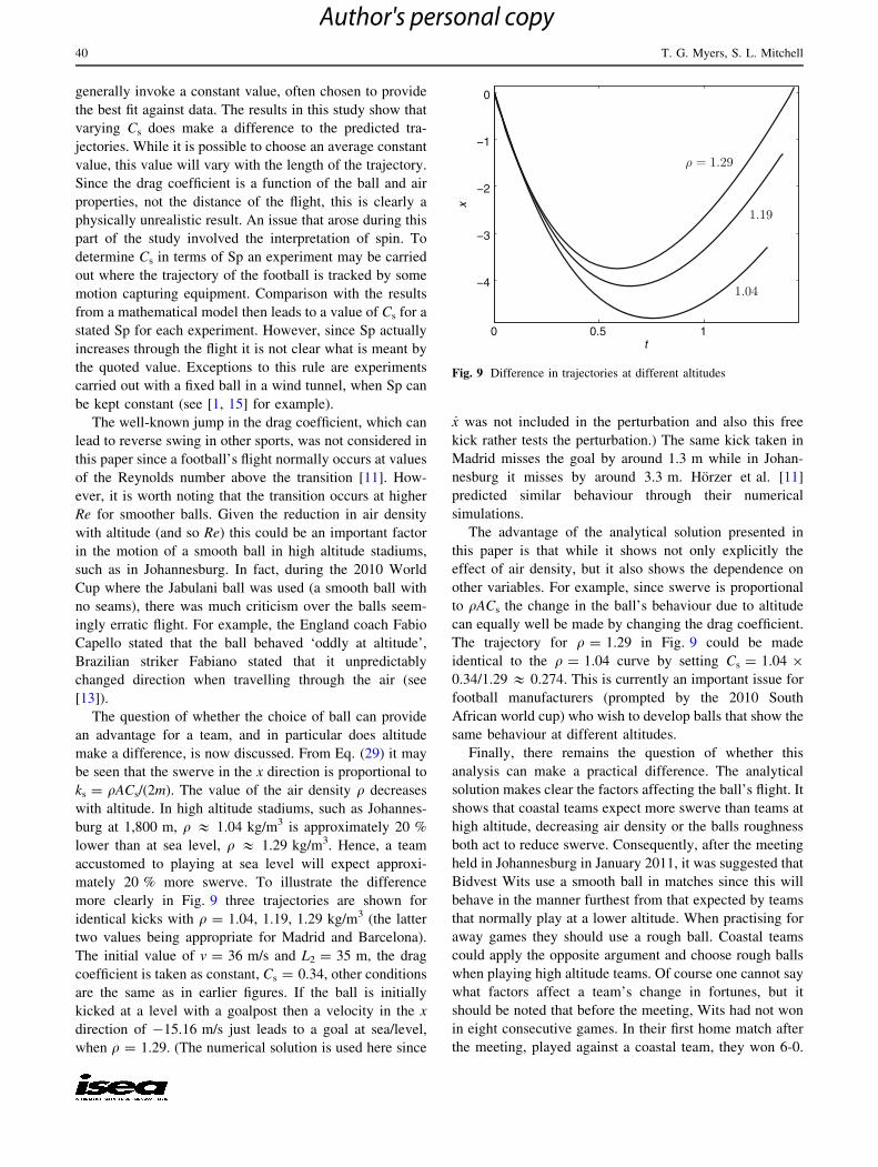
more clearly in Fig. 9 three trajectories are shown for

identical kicks with q = 1.04, 1.19, 1.29 kg/m3 (the latter

two values being appropriate for Madrid and Barcelona).

The initial value of v = 36 m/s and L2 = 35 m, the drag

coefficient is taken as constant, Cs = 0.34, other conditions

are the same as in earlier figures. If the ball is initially

kicked at a level with a goalpost then a velocity in the x

direction of -15.16 m/s just leads to a goal at sea/level,

when q = 1.29. (The numerical solution is used here since

_x was not included in the perturbation and also this free

kick rather tests the perturbation.) The same kick taken in

Madrid misses the goal by around 1.3 m while in Johan-

nesburg it misses by around 3.3 m. Horzer et al. [11]

predicted similar behaviour through their numerical

simulations.

The advantage of the analytical solution presented in

this paper is that while it shows not only explicitly the

effect of air density, but it also shows the dependence on

other variables. For example, since swerve is proportional

to qACs the change in the ball’s behaviour due to altitude

can equally well be made by changing the drag coefficient.

The trajectory for q = 1.29 in Fig. 9 could be made

identical to the q = 1.04 curve by setting Cs = 1.04 9

0.34/1.29 & 0.274. This is currently an important issue for

football manufacturers (prompted by the 2010 South

African world cup) who wish to develop balls that show the

same behaviour at different altitudes.

Finally, there remains the question of whether this

analysis can make a practical difference. The analytical

solution makes clear the factors affecting the ball’s flight. It

shows that coastal teams expect more swerve than teams at

high altitude, decreasing air density or the balls roughness

both act to reduce swerve. Consequently, after the meeting

held in Johannesburg in January 2011, it was suggested that

Bidvest Wits use a smooth ball in matches since this will

behave in the manner furthest from that expected by teams

that normally play at a lower altitude. When practising for

away games they should use a rough ball. Coastal teams

could apply the opposite argument and choose rough balls

when playing high altitude teams. Of course one cannot say

what factors affect a team’s change in fortunes, but it

should be noted that before the meeting, Wits had not won

in eight consecutive games. In their first home match after

the meeting, played against a coastal team, they won 6-0.

0 0.5 1

−4

−3

−2

−1

0

t

x

Fig. 9 Difference in trajectories at different altitudes

40 T. G. Myers, S. L. Mitchell

Author's personal copy

Up to the end of the 2011 season they subsequently lost

only one home game which was a cup tie, where the home

team do not provide the ball. Unfortunately, they did not

fare so well at away games.

Acknowledgments The research of TGM was supported by the

Marie Curie International Reintegration Grant Industrial applications

of moving boundary problems, Grant No. FP7-256417 and Ministerio

de Ciencia e Innovacion Grant MTM2010-17162. SLM acknowledges

the support of the Mathematics Applications Consortium for Science

and Industry (MACSI, http://www.macsi.ul.ie) funded by the Science

Foundation Ireland Mathematics Initiative Grant 06/MI/005.

References

1. Asai T, Seo K, Kobayashi O, Sakashita R (2007) Fundamental

aerodynamics of the soccer ball. Sports Eng 10:101–110

2. Bray K, Kerwin D (2003) Modelling the flight of a soccer ball in

a direct free kick. J Sports Sci 21(2):75–85

3. Bray K, Kerwin D (2005) Simplified flight equations for a spin-

ning soccer ball. In: Science and football V: proceedings of the

5th world congress on science and football

4. Carre MJ, Goodwill SR, Haake SJ (2005) Understanding the

effect of seams on the aerodynamics of an association football.

J Mech Eng Sci 219:657–666

5. Carre MJ, Asai T, Akatsuka T, Hakke SJ (2002) The curve kick

of a football ll: flight through the air. Sports Eng 5:193–200

6. Dupeux G, Le Goff A, Qur D, Clanet C (2010) The spinning ball

spiral. New J Phys 12. doi:10.1088/1367-2630/12/9/093004

7. Goff JE, Carre MJ (2009) Trajectory analysis of a soccer ball. Am

J Phys 77(11):1020–1027

8. Goff JE, Carre MJ (2010) Soccer ball lift coefficients via tra-

jectory analysis. Eur J Phys 31:775–784

9. Griffiths I, Evans C, Griffiths N (2005) Tracking the flight of

a spinning football in three dimensions. Meas Sci Technol 16:

2056–2065

10. The history of soccer. http://www.soccerballworld.com/History.

htm#Early. Accessed 4 May 2011

11. Horzer S, Fuchs C, Gastinger R, Sabo A, Mehnem L, Martinek J,

Reichel M (2010) Simulation of spinning soccer ball trajectories

influenced by altitude, 8th conference of the International Sports

Engineering Association (ISEA). Procedia Eng 2:2461–2466

12. Jabulani. http://www.jabulaniball.com/. Accessed 4 May 2011

13. Adidas Jabulani. http://en.wikipedia.org/wiki/Adidas_Jabulani.

Accessed 4 May 2011

14. Oggiano L, Sætran L (2010) Aerodynamics of modern soccer

balls. Procedia Eng 2:2473–2479

15. Passmore M, Tuplin S, Spencer A, Jones R (2008) Experimental

studies of the aerodynamics of spinning and stationary footballs.

Proc Inst Mech Eng Part C J Mech Eng Sci 222(2):195–205

16. Wesson J (2002) The science of soccer. IoP Pub. Ltd., Bristol

Mathematics of soccer ball motion 41

Author's personal copy