BPEA Conference Drafts, September 7–8, 2017

Investmentless Growth: An Empirical Investigation

Germán Gutiérrez, New York University

Thomas Philippon, New York University

Conflict of Interest Disclosure: The authors did not receive financial support from any firm or

person for this paper or from any firm or person with a financial or political interest in this paper.

They are currently not officers, directors, or board members of any organization with an interest

in this paper. No outside party had the right to review this paper prior to circulation.

Investment-less Growth:

An Empirical Investigation∗

Germán Gutiérrez† and Thomas Philippon‡

September 2017

Abstract

We analyze private �xed investment in the U.S. over the past 30 years. We show that invest-

ment is weak relative to measures of pro�tability and valuation � particularly Tobin's Q, and

that this weakness starts in the early 2000's. There are two broad categories of explanations:

theories that predict low investment along with low Q, and theories that predict low investment

despite high Q. We argue that the data does not support the �rst category, and we focus on

the second one. We use industry-level and �rm-level data to test whether under-investment

relative to Q is driven by (i) �nancial frictions, (ii) changes in the nature and/or localization of

investment (due to the rise of intangibles, globalization, etc), (iii) decreased competition (due

to technology, regulation or common ownership), or (iv) tightened governance and/or increased

short-termism. We do not �nd support for theories based on risk premia, �nancial constraints,

safe asset scarcity, or regulation. We �nd some support for globalization; and strong support for

the intangibles, competition and short-termism/governance hypotheses. We estimate that the

rise of intangibles explains 25-35% of the drop in investment; while Concentration and Gover-

nance explain the rest. Industries with more concentration and more common ownership invest

less, even after controlling for current market conditions and intangibles. Within each industry-

year, the investment gap is driven by �rms owned by quasi-indexers and located in industries

with more concentration and more common ownership. These �rms return a disproportionate

amount of free cash �ows to shareholders. Lastly, we show that standard growth-accounting

decompositions may not be able to identify the rise in markups.

∗We are grateful to Bob Hall, Janice Eberly, Olivier Blanchard, Toni Whited, René Stulz, Martin Schmalz, BoyanJovanovic, Tano Santos, Charles Calomiris, Glenn Hubbard, Holger Mueller, Alexis Savov, Philipp Schnabl, RalphKoijen, Ricardo Caballero, Emmanuel Farhi, Viral Acharya, and seminar participants at Columbia University andNew York University for stimulating discussions†New York University‡New York University, CEPR and NBER

1

In his March 2016 letter to the executives of S&P 500 �rms, BlackRock's CEO Laurence Fink

argues that, �in the wake of the �nancial crisis, many companies have shied away from investing in

the future growth of their companies. Too many companies have cut capital expenditure and even

increased debt to boost dividends and increase share buybacks.� The decline in investment has been

discussed in policy papers [Furman, 2015, IMF, 2014, Vashakmadze et al., 2017]; as well as academic

papers (see, for example, Hall [2015], Alexander and Eberly [2016], Fernald et al. [2017]). And it

appears to a�ect not only the U.S. but also Europe and other emerging markets [Bussiere et al.,

2015, Buca and Vermeulen, 2015, Dottling et al., 2017, Lewis et al., 2014, Kose et al., 2017].

This paper presents systematic evidence on the extent of the investment puzzle and provides

a preliminary assessment of the potential explanations. We clarify some of the theory and the

empirical evidence; and test whether alternate theories of under-investment are supported by the

data. The main contributions of the paper are to show that: (i) the lack of investment represents

a reluctance to invest despite high Tobin's Q; and (ii) this investment wedge is linked to the rise

of intangibles, decreased competition and changes in governance that encourage payouts instead of

investment.

We emphasize that the goal of our paper is not to establish causality of a particular mechanism.

Instead, we present a broad overview of the available evidence and we review the proposed theoretical

explanations. We spend much time and e�ort connecting the results at the �rm-level, at the

industry-level, and in the aggregate, and we discuss the macro-economic implications of our �ndings.

The goal of our paper is to broadly test a large set of theories regarding investment dynamics. We

�nd that competition and governance are promising explanations but we do not try to establish

causality. We address the causality issue using a combination of instrumental variables and natural

experiments in two related papers (Gutiérrez and Philippon [2017a] for competition and Gutiérrez

and Philippon [2017b] for governance and short-termism).

Approach Throughout the paper, we use Q-theory as a measurement tool to distinguish between

two broad types of shocks: (i) shocks that �t the Q equation, and therefore predict low investment

along with low Tobin's Q; and (ii) shocks that change the Q equation and therefore predict low

investment despite high Tobin's Q. The �rst category includes shocks to risk aversion and expected

growth. The standard Q-equation holds under these shocks, so the only way they can explain low

investment is by predicting low values of Q. The second category ranges from credit constraints

to oligopolistic competition, and implies a shift in the �rst order condition for optimal investment.

Such shocks create a gap between Q and investment due to di�erences between average and marginal

Q (e.g., market power, growth options) and/or di�erences between �rm value and the manager's

objective function (e.g., governance, short-termism).

To di�erentiate between these two broad types of shocks, we study the relationship between

private �xed investment and Q. We �nd that investment is weak relative to measures of pro�tability

and valuation � particularly Tobin's Q. Time e�ects from industry- and �rm-level panel regressions

on Q suggest that this weakness starts around 2000. This is true controlling for �rm age, size,

2

and pro�tability; focusing on subsets of industries; and even considering tangible and intangible

investment separately. Given these results, we discard shocks that predict low investment along

with low Q; and focus on theories that create a gap between Q and investment. This still leaves a

large set of potential explanations � out of which we consider the following eight (grouped into four

broad categories):1

• Financial frictions

1. External �nance

2. Bank dependence

3. Safe asset scarcity

• Changes in the nature and/or localization of investment

4. Intangibles

5. Globalization

• Decreased Competition

6. Regulation

7. Market power due to other factors

• Tighter Governance

8. Ownership and Shareholder Activism

Testing these hypotheses requires a lot of data, at di�erent levels of aggregation. Some are industry-

level theories (e.g., competition), some �rm-level theories (e.g., ownership), and some theories that

can be tested at the industry level and at the �rm level. We gather industry investment data from

the BEA and �rm investment data from Compustat; as well as additional data needed to test each

of the eight hypotheses.

For instance, for market power, we obtain (Compustat and Census) measures of �rm entry, �rm

exit, price-cost margins, and concentration (including `traditional' and common ownership-adjusted

Her�ndahls2, as well as concentration ratios de�ned as the share of sales and market value of the

Top 4, 8, 20 and 50 �rms in each industry). For governance and short-termism, we use Brian

Bushee's institutional investor classi�cation [Bushee, 2001]. The classi�cation identi�es Quasi-

indexer, Transient and Dedicated institutional investors based on the turnover and diversi�cation

of their holdings. Dedicated institutions have large, long-term holdings in a small number of �rms.

Quasi-indexers have diversi�ed holdings and low portfolio turnover, consistent with a passive buy-

and-hold strategy. Transient owners have high diversi�cation and high portfolio turnover. Sample

1See Section 2 for a detailed discussion of these hypotheses.2We follow Salop and O'Brien [2000] and Azar et al. [2016b] to compute the common ownership-adjusted Her�nd-

ahl, which accounts for anti-competitive incentives due to common ownership. See Section 2 for additional details

3

Dedicated, Quasi-indexer and Transient institutions include Berkshire Hathaway, Vanguard and

Credit Suisse, respectively. See Section 3 for additional details.

Firm- and industry-data are not readily comparable because they di�er in their coverage; and

in their de�nitions of investment and capital. As a result, we spent a fair amount of time simply

reconciling and understanding the various data sources. The key conclusions are summarized in

Section 3 and in the Appendix. The �nal datasets are not entirely comparable, primarily due to

di�erences between accounting and economic values. But they do exhibit similar trends. And our

conclusions are robust across datasets and levels of aggregation.

Conclusions We test whether each of the eight hypothesis is supported by the data through

industry- and �rm-level panel regressions. We use the Erickson et al. [2014] cumulant estimator

to control for `classical' errors-in-variables problems in Q, and discuss key sources measurement

error where appropriate. We �nd strong support for the Market power, Governance and Intangibles

hypotheses:

• Market power and Governance: At the industry level, we �nd that industries with more

quasi-indexer institutional ownership and less competition (as measured by higher `traditional'

and common ownership-adjusted Her�ndahls, as well as higher price-cost margins) invest less.

These results are robust to controlling for intangible intensity, �rm age as well as Q. The de-

crease in competition is supported by a growing literature,3 though the empirical implications

for investment have not been recently studied (to our knowledge). Similarly, the mechanisms

through which quasi-indexer institutional ownership impacts investment remain to be fully un-

derstood: while such ownership may eliminate empire-building by improving governance (e.g.,

Appel et al. [2016a]), it may also increase short-termism (e.g., Asker et al. [2014], Almeida

et al. [2016], Bushee [1998]) � both of which could lead to higher payouts and less investment.

At this point, we are unable to di�erentiate between these two hypotheses empirically. We

simply show that �rms with higher passive institutional ownership have higher payouts and

lower investment. Relatedly, Gutiérrez [2017] uses industry-level data to study the evolution

of labor and pro�t shares across advanced economies. He shows that labor shares decreased

and pro�t shares increased only in the U.S., while they remained stable in the rest of the

World. The rise in markups explains the majority of the decrease in the U.S. labor share since

the late 1990s.

Firm-level results are consistent with industry-level results. They suggest that within each

industry-year and controlling for Q, �rms with higher quasi-indexer institutional ownership

invest less; and �rms in industries with less competition also invest less.

3For instance, the 2016 issue brief of the Council of Economic Advisers �reviews three sets of trends that are

broadly suggestive of a decline in competition: increasing industry concentration, increasing rents accruing to a few

�rms, and lower levels of �rm entry and labor market mobility.� (see also Decker et al. [2015] and Grullon et al.[2016]).

4

• Intangibles: The rise of intangibles can a�ect investment in two primary ways: First, intangi-ble investment is di�cult to measure. Under-estimation of I would lead to under-estimation of

K, and therefore over-estimation ofQ; which could translate to an `observed' under-investment

at industries with a higher share of intangibles. Second, intangible assets might be more dif-

�cult to accumulate. A rise in the relative importance of intangibles could therefore lead to

a higher equilibrium value of Q even if intangibles are correctly measured. Peters and Taylor

[2016] and Alexander and Eberly [2016] study the relationship between Q and intangible in-

vestment. Consistent with their work, we �nd that industries with a rising share of intangibles

exhibit lower investment. We �nd that the rise of intangibles can explain a quarter to a third

of the observed investment gap. Yet we are still left with large, persistent residuals after

2000 � residuals that are strongly correlated with increased concentration and quasi-indexer

ownership.4

None of the other theories (e.g., credit constraints) appear to be supported by the data. They often

exhibit the `wrong' and/or inconsistent signs; or are not statistically signi�cant. Globalization also

does not appear to be a primary driver of under-investment. Industries with higher foreign pro�ts

invest less in the US, as expected, but �rm level investment does not depend on the share of foreign

pro�ts.

Macro-implications To conclude, we study the implications of our �ndings against recent work

in the macro-literature. In particular, Fernald et al. [2017] rely on a quantitative growth-accounting

decomposition to study the output shortfall in the US following the Great Recession. They con-

clude that the shortfall is explained by slower TFP growth and decreased labor force participation.

Focusing on the capital stock, they argue that �although capital formation has been below par [since

2009], so has output growth, and by 2016, the capital/output ratio was in line with its long-term

trend.� Their �ndings have direct implications for our conclusions. Yet the underlying driver (a

potential increase in market power) may be confounded in the macro series.

To test this hypothesis, we simulate macro-series under rising mark-ups using the model of

Jones and Philippon [2016],5 and study whether growth-accounting decompositions recover the

appropriate shocks. We �nd that a rise in mark-ups decreases output, capital, labor and K/Y (as

expected). `Measured' TFP decreases slightly when using standard growth approaches (such as

those of Fernald et al. [2017] and Fernald [2014]) and adjusting for changes in the capital share.

4It is also worth emphasizing, as Peters and Taylor [2016] do, that Q explains intangible investment relativelywell, and works even better when both tangible and intangible investments are combined. This is exactly as thetheory would predict. Moreover, intangible investment exhibits roughly the same weakness as tangible investmentstarting around 2000. Properly accounting for intangible investment is clearly a �rst order empirical issue, but, as faras we can tell, it does not lessen the puzzle that we document. See Döttling and Perotti [2017] for related evidence

5Jones and Philippon [2016] explore the macro-economic consequences of decreased competition in a standardDSGE model with time-varying parameters and an occasionally binding zero lower bound. They show that the trenddecrease in competition can explain the joint evolution of investment, Q, and the nominal interest rate. Absent thedecrease in competition, they �nd that the U.S. economy would have escaped the ZLB by the end of 2010 and thatthe nominal rate in 2016 would be close to 2%.

5

Table 1: Current Account of Non �nancial Sector

Value in 2014 ($ billions)

Name Notation Corporate1 Non corporate2 Business1+2

Gross Value Added PtYt $8,704 $3,177 $11,881

Net Fixed Capital at Rep. Cost Pkt Kt $14,813 $6,155 $20,968

Consumption of Fixed Capital δtPkt Kt $1,283 $299 $1,581

Net Operating Surplus PtYt −WtNt − T yt − δtPkt Kt $1,683 $1,723 $3,406

Gross Fixed Capital Formation Pkt It $1,626 $367 $1,993

Net Fixed Capital Formation Pkt (It − δtKt) $343 $68 $411

Applying the cycle-trend-irregular decomposition of Fernald et al. [2017], we �nd that the de-

composition largely absorbs the rise in market power � and therefore appears unable to separately

identify declines in K/Y driven by (long term) changes in market power from those driven by other

factors. As a result, such decompositions may confound a rise in market power with a decrease

in TFP , and conclude that decreases in output are due to lower TFP rather than higher market

power.

The remainder of this paper is organized as follows. Section 1 presents �ve important facts

about the Non �nancial sector and its investment. Section 2 discusses the theories that may explain

under-investment relative to Q and reviews the related literature. Section 3 describes the data

used to test our eight hypotheses. Section 4 discusses the methodology and results of our analyses.

Section 5 drills-down to provide detailed discussions of three hypotheses: (i) increased concentration,

particularly as it relates to `Superstar' �rms; (ii) the rise of intangibles; and (iii) the e�ect of safe

asset scarcity on investment. Section 6 discusses the macro-economic implications of our results;

and Section 7 concludes.

1 Five Facts about US Non �nancial Sector

We present �ve important facts related to investment by the US non �nancial sector in recent years.

We focus on the non �nancial sector for three main reasons. First, this sector is the main source

of nonresidential investment. Second, we can roughly reconcile aggregate data from the Financial

Accounts of the United States (Financial Accounts) with industry-level investment data from the

BEA (which includes residential and non residential investment, as well as investment in intellectual

property). Last, we can use data on the market value of bonds and stocks for the non �nancial

corporate sector to disentangle various theories of secular stagnation.

1.1 Fact 1: The Non �nancial Business Sector is Pro�table but does not Invest

Table 1 summarizes some key facts about the balance sheet and current account of the non �nancial

corporate, non �nancial non corporate and non �nancial business sectors.

6

Figure 1: Net Operating Return, by Sector

.1.1

5.2

.25

.3

1970 1980 1990 2000 2010year

Non Financial Corporate Non Financial Non CorporateNon Financial Business

Note: Annual data, by Non �nancial Business sector.

One reason investment might be low is that pro�ts might be low. This, however, is not the case.

Figure 1 shows the operating return on capital of the non �nancial corporate, non �nancial non

corporate and non �nancial business sector, de�ned as net operating surplus over the replacement

cost of capital:

Net Operating Return =PtYt − δtP kt Kt −WtNt − T yt

P kt Kt(1)

As shown, the operating return for corporates has been quite stable over time while the operating

return of non corporates has increased substantially since 1990. For corporates, the yearly average

from 1971 to 2015 is 10.5%, with a standard deviation of only one percentage point. The minimum is

8.1% and the maximum 12.6%. In 2015, the operating return was 11.2%, very close to the historical

maximum. For non corporates, the yearly average from 1971 to 2015 is 24%, while the average since

2002 has been 27%. The maximum is 29%, equal to the operating return observed every year since

2012. A striking feature is that the net operating margin was not severely a�ected by the Great

Recession, and has been consistently near its highest value since 2011 for both Corporates and Non

corporates.6

But �rms do not invest the same fraction of their operating returns as they used to. Figure 2

shows the ratio of net investment to net operating surplus for the non �nancial business sector:

NI/OS =P kt (It − δtKt)

PtYt − δtP kt Kt −WtNt − T yt(2)

The average of the ratio between 1962 and 2001 is 20%. The average of the ratio from 2002 to

6Gomme et al. [2011] implement a related calculation of the after-tax return to business capital and �nd similarconclusions.

7

Figure 2: Net Investment Relative to Net Operating Surplus

0.1

.2.3

1960 1970 1980 1990 2000 2010year

Note: Annual data for Non �nancial Businesses (Corporate and Non corporate).

2015 is only 10%.7 Current investment is low relative to operating margins. Similar patterns are

observed when separating corporates and non corporates.

1.2 Fact 2: Investment is low relative to Q

Of course, economic theory does not say that NI/OS should be constant over time. Investment

should depend on expected future operating surplus, on the capital stock, and the cost of funding

new investment; it should rely on a comparison of expected returns on capital and funding costs.

The neoclassical theory of investment � developed in Jorgenson [1963], Brainard and Tobin [1968]

and Tobin [1969], among others � captures this trade-o�.8

Consider a �rm that chooses a sequence of investment to maximize its value. Let Kt be capital

available for production at the beginning of period t and let µt be the pro�t margin of the �rm. The

basic theory assumes perfect competition so the �rm takes µ as given. In equilibrium, µ depends

on productivity and production costs (wages, etc.). The �rm's program is then

Vt (Kt) = maxIt

µtPtKt − P kt It −γ

2P kt Kt

(ItKt− δt

)2

+ Et [Λt+1Vt+1 (Kt+1)] , (3)

where P kt is the price of investment goods and γ controls adjustment costs. Given our homogeneity

assumptions, it is easy to see that the value function is homogeneous in K. We can then de�ne

7Note that 2002 is used for illustration purposes only; the cut-o� is not based on a formal statistical analysis.8See Dixit and Pindyck [1994], among others, for a rigorous treatment of the theory of investment with non-convex

adjustment costs.

8

Vt ≡ VtKt

which solves

Vt = maxx

µtPt − P kt (xt + δt)−γ

2P kt x

2 + (1 + xt)Et [Λt+1Vt+1] , (4)

where xt ≡ ItKt− δt is the net investment rate. The resulting �rst order condition for the net

investment rate is

xt =1

γ(Qt − 1) , (5)

where

Qt ≡Et [Λt+1Vt+1]

P kt=

Et [Λt+1Vt+1]

P kt Kt+1. (6)

Q is the ex-dividend market value of the �rm divided by the replacement cost of its capital stock.

Clearly, Q is just one �rst-order condition satis�ed by the �rm � with another condition driving

demand for the �rm's output; and several other conditions needed to close the standard model. As

a result, Q is not a causal force of investment. It is simply a useful (endogenous) measure to classify

shocks over time. To build our empirical measures of Q, we de�ne

Q =V e + (L− FA)− Inventories

PkK(7)

where V e is the market value of equity, L are the liabilities (mostly measured at book values, but

this is a rather small adjustment, see Hall [2001]), and FA are �nancial assets. Note that the BEA

measure of K now includes intangible assets (including software, R&D, as well as entertainment,

literary, and artistic originals). As a result, our measure of Q is lower than in the previous literature.

Because �nancial assets and liabilities contain large residuals, we also compute another measure of

Q:

Qmisc = Q+Amisc − Lmisc

PkK(8)

where Amisc and Lmisc are the miscellaneous assets and liabilities recorded in the Financial Accounts.

Since Amisc > Lmisc, it follows that Qmisc > Q. It is unclear which measure is more appropriate.

Figure 3 shows the evolution of Q for the non �nancial corporate sector. As shown, Q is high

according to both measures, by historical standards. This is consistent with the rapid rise in

corporate pro�ts shown in Figure 1 and the rise in net savings (not shown).

This leads us to our main conclusion: investment is low relative to Q. The top chart in Figure 4

shows the aggregate net investment rate for the non �nancial business sector along with the �tted

value for a regression on (lagged) Q from 1990 to 2001. The bottom chart shows the regression

residuals (for each period and cumulative) from 1990 to 2015. Both charts clearly show that in-

vestment has been low relative to Q since sometime in the early 2000's.9 By 2015, the cumulative

under-investment is more than 10% of capital.10

9By de�nition of OLS, the cumulative residual for 2001 is zero, but the under-investment from then on is striking10We focus on the past 25 years because measures of Q based on equity are not always stable and therefore do not �t

long time series. This is a well known fact that might be due to long run changes in technology and/or participation in

9

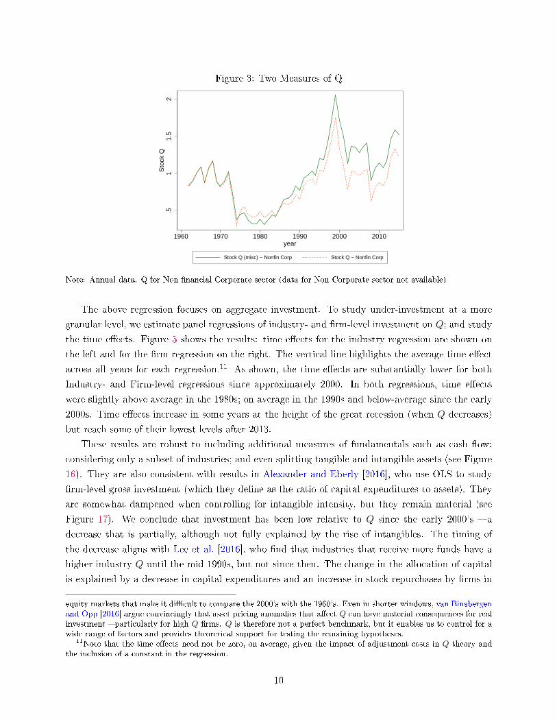
Figure 3: Two Measures of Q

.51

1.5

2S

tock

Q

1960 1970 1980 1990 2000 2010year

Stock Q (misc) − Nonfin Corp Stock Q − Nonfin Corp

Note: Annual data. Q for Non �nancial Corporate sector (data for Non Corporate sector not available)

The above regression focuses on aggregate investment. To study under-investment at a more

granular level, we estimate panel regressions of industry- and �rm-level investment on Q; and study

the time e�ects. Figure 5 shows the results: time e�ects for the industry regression are shown on

the left and for the �rm regression on the right. The vertical line highlights the average time e�ect

across all years for each regression.11 As shown, the time-e�ects are substantially lower for both

Industry- and Firm-level regressions since approximately 2000. In both regressions, time e�ects

were slightly above average in the 1980s; on average in the 1990s and below-average since the early

2000s. Time e�ects increase in some years at the height of the great recession (when Q decreases)

but reach some of their lowest levels after 2013.

These results are robust to including additional measures of fundamentals such as cash �ow;

considering only a subset of industries; and even splitting tangible and intangible assets (see Figure

16). They are also consistent with results in Alexander and Eberly [2016], who use OLS to study

�rm-level gross investment (which they de�ne as the ratio of capital expenditures to assets). They

are somewhat dampened when controlling for intangible intensity, but they remain material (see

Figure 17). We conclude that investment has been low relative to Q since the early 2000's � a

decrease that is partially, although not fully explained by the rise of intangibles. The timing of

the decrease aligns with Lee et al. [2016], who �nd that industries that receive more funds have a

higher industry Q until the mid-1990s, but not since then. The change in the allocation of capital

is explained by a decrease in capital expenditures and an increase in stock repurchases by �rms in

equity markets that make it di�cult to compare the 2000's with the 1960's. Even in shorter windows, van Binsbergenand Opp [2016] argue convincingly that asset pricing anomalies that a�ect Q can have material consequences for realinvestment � particularly for high Q �rms. Q is therefore not a perfect benchmark, but it enables us to control for awide range of factors and provides theoretical support for testing the remaining hypotheses.

11Note that the time e�ects need not be zero, on average, given the impact of adjustment costs in Q theory andthe inclusion of a constant in the regression.

10

Figure 4: Net Investment vs. Q0

.01

.02

.03

.04

NI/K

1990 1995 2000 2005 2010 2015year

Net Investment Fitted values

Net investment (actual and predicted with Q)

−.1

−.0

50

Reg

ress

ion

resi

dual

s

1990 1995 2000 2005 2010 2015year

Cumulative gap Residual

Prediction residuals (by period and cumulative)

Note: Annual data. Net investment for Non �nancial Business sector.

11

high Q industries since the mid-1990s.

Figure 5: Time e�ects from Industry and Firm-level regressions

year==1980year==1981year==1982year==1983year==1984year==1985year==1986year==1987year==1988year==1989year==1990year==1991year==1992year==1993year==1994year==1995year==1996year==1997year==1998year==1999year==2000year==2001year==2002year==2003year==2004year==2005year==2006year==2007year==2008year==2009year==2010year==2011year==2012year==2013year==2014

−.1 −.08 −.06 −.04 −.02 0

Industry−level time effects (BEA)year==1980year==1981year==1982year==1983year==1984year==1985year==1986year==1987year==1988year==1989year==1990year==1991year==1992year==1993year==1994year==1995year==1996year==1997year==1998year==1999year==2000year==2001year==2002year==2003year==2004year==2005year==2006year==2007year==2008year==2009year==2010year==2011year==2012year==2013year==2014year==2015

−.6 −.4 −.2 0

Firm−level time effects (Compustat)

Note: Time �xed e�ects from errors-in-variables panel regressions (Erickson et al. [2014]) of industry net investmenton median Log-Q (left) and Log((CAPX+R&D)/AT) on �rm-level Log-Q (right) as well as a control for �rm age. Allvariables are de-meaned over the regression period at the industry- and �rm-level, respectively. Industry investmentdata from BEA; Q and �rm investment from Compustat. See Section 4.2.1 for additional details on the regressionapproach.

1.3 Fact 3: Depreciation and Relative Investment Prices Have Remained Stable

Since 2000

The decrease in net investment could be the result of changes in the depreciation rate. To test

this, Figure 6 shows the gross investment rate, the net investment rate and the depreciation rate

for the non �nancial corporate sector on the top, and the non �nancial non corporate sector on the

bottom. Note that these series include residential structures, but their contribution is relatively

small for non �nancial businesses. The gross investment rate is de�ned as the ratio of `Gross �xed

capital formation with equity REITs' to lagged capital. Depreciation rates are de�ned as the ratio

of `consumption of �xed capital, equipment, software, and structures, including equity REIT' to

lagged capital; and net investment rates as the gross investment rate minus the depreciation rate.

In the non corporate sector, depreciation is stable and net investment follows gross investment.

The evolution is more complex in the corporate sector. There was a secular increase in depreciation

from 1960 until 2000, driven primarily by a shift in the composition of corporate investment (from

12

Figure 6: Investment and Depreciation Rate for Non �nancial Business Sector

0.0

5.1

.15

1960 1970 1980 1990 2000 2010year

Net I/K Gross I/KDepreciation/K

Non financial Corporate

0.0

5.1

.15

1960 1970 1980 1990 2000 2010year

Net I/K Gross I/KDepreciation/K

Non financial Non Corporate

Note: Annual data. Non �nancial Corporate sector on the top, Non �nancial Non corporate sector on the bottom.

structures and equipment to intangibles). As a result, the trend in net investment is signi�cantly

lower than the trend in gross investment. Since 2000, however, the share of intangible assets has

remained �at such that depreciation has been more stable, and, if anything, it has decreased. The

drop in net investment over the past 15 years is therefore due to a drop in gross investment, not

a rise in depreciation. Because the corporate sector contributes the lion share of investment, the

aggregate �gure for the combined non-�nancial sector resembles the top panel (see Table 1).

Figure 7 shows the relative price of nonresidential investment goods and equipment, de�ned

as the ratio of the `Fixed investment: Nonresidential (implicit price de�ator)' to the `Personal

consumption expenditures (implicit price de�ator)'. As shown, the relative price of capital decreased

drastically since the 1980s, but has remained relatively stable after 2000. Thus, the recent under-

investment is unlikely to be driven by changes in investment prices.

13

Figure 7: Relative price of investment goods

11.

21.

41.

6R

elat

ive

pric

e: N

onre

side

ntia

l

1960 1970 1980 1990 2000 2010year

Note: Annual data. Relative price of investment goods de�ned as the ratio of the `Fixed investment: Nonresidential(implicit price de�ator)' to the `Personal consumption expenditures (implicit price de�ator)'

1.4 Fact 4: Firm Entry has Decreased

Figure 8 shows two measures of �rm entry: the establishment entry and exit rates as reported by

the U.S. Census Bureau's Business Dynamics Statistics (BDS); and the average number of �rms

by industry in Compustat. The downward trend in business dynamism has been highlighted by

numerous papers (e.g., Decker et al. [2014]), and it has been particularly severe in recent years.

In fact, Decker et al. [2015] argue that, whereas in the 1980s and 1990s declining dynamism was

observed in selected sectors (notably retail), the decline was observed across all sectors in the 2000s,

including the traditionally high-growth information technology sector.

The Census data provides a comprehensive view of entry and exit. This is not the case with

Compustat since it covers mostly the large, publicly-traded companies. For instance, in the early

1990s, we see a large increase in Compustat �rms, driven primarily by �rms going public. Since then,

both charts provide strong evidence of a decline in the number of �rms. The decrease in Compustat

�rms is particularly notable once normalizing for GDP: the number of �rms in Compustat today is

approximately the same as in 1975 yet GDP is 3x larger.

14

Figure 8: Firm entry, exit and number of �rms

.08

.1.1

2.1

4.1

6

1980 1985 1990 1995 2000 2005 2010 2015year

Entry rate (Census) Exit rate (Census)

Establishment entry and exit rates (Census)

6080

100

120

140

1980 1985 1990 1995 2000 2005 2010 2015year

Average number of firms by industry (Compustat)

Note: Annual data.

The Compustat and Census patterns above appear quite di�erent. However, focusing on the

post-2000 period (the main period of interest) and the sectors for which Compustat provides good

coverage, we �nd signi�cant similarities. Figure 9 shows the 3-year log change in the number of

�rms based on Compustat and the number of establishments based on Census BDS data (excluding

agriculture and construction for which Compustat provides limited coverage). As shown, changes

in the number of �rms are roughly similar across all sectors, including manufacturing, mining and

retail which are the main contributors of investment.

15

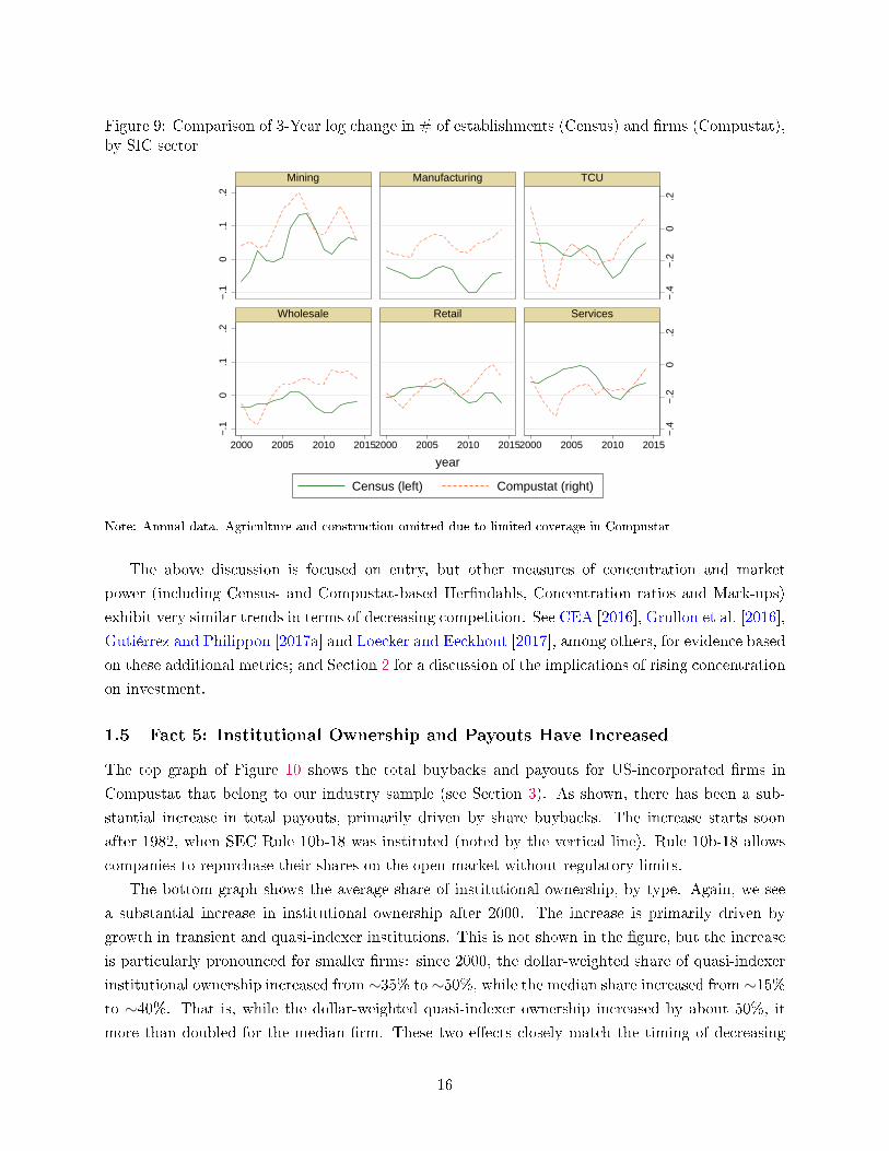
Figure 9: Comparison of 3-Year log change in # of establishments (Census) and �rms (Compustat),by SIC sector

−.4

−.2

0.2

−.4

−.2

0.2

−.1

0.1

.2−

.10

.1.2

2000 2005 2010 20152000 2005 2010 20152000 2005 2010 2015

Mining Manufacturing TCU

Wholesale Retail Services

Census (left) Compustat (right)

year

Note: Annual data. Agriculture and construction omitted due to limited coverage in Compustat

The above discussion is focused on entry, but other measures of concentration and market

power (including Census- and Compustat-based Her�ndahls, Concentration ratios and Mark-ups)

exhibit very similar trends in terms of decreasing competition. See CEA [2016], Grullon et al. [2016],

Gutiérrez and Philippon [2017a] and Loecker and Eeckhout [2017], among others, for evidence based

on these additional metrics; and Section 2 for a discussion of the implications of rising concentration

on investment.

1.5 Fact 5: Institutional Ownership and Payouts Have Increased

The top graph of Figure 10 shows the total buybacks and payouts for US-incorporated �rms in

Compustat that belong to our industry sample (see Section 3). As shown, there has been a sub-

stantial increase in total payouts, primarily driven by share buybacks. The increase starts soon

after 1982, when SEC Rule 10b-18 was instituted (noted by the vertical line). Rule 10b-18 allows

companies to repurchase their shares on the open market without regulatory limits.

The bottom graph shows the average share of institutional ownership, by type. Again, we see

a substantial increase in institutional ownership after 2000. The increase is primarily driven by

growth in transient and quasi-indexer institutions. This is not shown in the �gure, but the increase

is particularly pronounced for smaller �rms: since 2000, the dollar-weighted share of quasi-indexer

institutional ownership increased from ∼35% to ∼50%, while the median share increased from ∼15%to ∼40%. That is, while the dollar-weighted quasi-indexer ownership increased by about 50%, it

more than doubled for the median �rm. These two e�ects closely match the timing of decreasing

16

investments at the aggregate level.

Figure 10: Payouts and Institutional ownership

0.0

2.0

4.0

6.0

8

1970 1975 1980 1985 1990 1995 2000 2005 2010 2015year

Payouts/Assets Buybacks/Assets

Share Buybacks and Payouts

0.2

.4.6

1980 1985 1990 1995 2000 2005 2010 2015year

All institutions Quasi−IndexerDedicated Transient

Average share of institutional ownership, by type

Notes: Annual data for all US incorporated �rms in our Compustat sample. Results are similar when includingforeign-incorporated �rms. The vertical line in the �rst graph highlights the passing of SEC rule 10b-18, which allowscompanies to repurchase their shares on the open market without regulatory limits.

2 What might explain the under-investment?

Section 1 shows that investment is low relative to Q. This section outlines the theories that might

explain the investment gap and, in so doing, provides a broad review of the investment literature.

2.1 Theory

The basic Q-equation (5) says that Q should be a su�cient statistic for investment, while equation

(6) equates Q with the average market to book value. This theory is based on the following

17

assumptions [Hayashi, 1982]:

• no �nancial constraints;

• shareholder value maximization;

• constant returns to scale and perfect competition.

The Q-theory has been tested empirically by a large literature. Early results have been somewhat

disappointing. With aggregate US data, the basic Q-equation �ts poorly, leaves large unexplained

residuals correlated with cash �ows, and implies implausible parameters for the adjustment cost

function. Hassett and Hubbard [1997] and Caballero [1999] provide reviews of the early literature.

Several theories have emerged to explain these failures � namely market power [Abel and Eberly,

1994], non-convex adjustment costs [Caballero and Engle, 1999] and �nancial frictions [Bernanke and

Gertler, 1989]. However, none of these is fully satisfactory. The evidence for constant returns and

price taking seems quite strong [Hall, 2003]. Adjustment costs are certainly not convex at the plant

level, but it is not clear that this really matters at the industry level or in the aggregate [Thomas,

2002, Hall, 2004], but this is still a controversial issue [Bachmann et al., 2013]. Gomes [2001] shows

that Q should capture most investment dynamics even when there are credit constraints. And

heterogeneity and aggregation do not seem to create strong biases [Hall, 2004].

A fourth explanation � measurement error in Q � has found strong support in the recent litera-

ture. Work in the 1990s and early 2000s emphasizes measurement error in market value of equity as

a substantial culprit for the empirical failure of the investment equation [Gilchrist and Himmelberg,

1995, Cumins et al., 2006, Erickson and Whited, 2000]. Erickson and Whited [2000] and Erick-

son and Whited [2006] in particular use GMM estimators to purge Q from measurement errors.

They �nd that only 40 percent of observed variations are due to fundamental changes, implying

that market values contain large `measurement errors'. Q-theory performs substantially better once

controlling for such `classical' measurement error, and residuals are no longer correlated with cash

�ows. Recently, Peters and Taylor [2016] emphasizes measurement error in intangible capital, and

shows that properly accounting for intangibles substantially improves the performance of Q-theory

(although, as we discuss later, this is in part due to their choice of the empirical proxy for traditional

Q).

We take these theories � and the implied deviations between Q and investment � seriously.

We control for `classical' errors-in-variables problems using the cumulant estimator of Erickson

et al. [2014]; and use empirical proxies for the remaining theories to test whether they can explain

(under-)investment. In other words, we use Q-theory as a benchmark and a useful way to sort

the explanations into two groups: those where Q-theory �ts (e.g. changes in risk premia, expected

demand or technology), and those that imply a divergence between Q and investment (e.g., changes

in market power). It is clear, however, that Q is an endogenous variable and not an independent

driver of investment. The following section details the speci�c hypotheses (i.e., variations of these

theories) that we consider.

18

The approach we take in this paper does not allow us to to prove a causal relationship between

a particular factor and investment. We deal with causality issues in two companion papers. To

quickly summarize, Gutiérrez and Philippon [2017a] focuses on market power. It clari�es the deep

endogeneity issue coming from endogenous entry; and proposes natural experiments (based on

increased competition from China) and instrumental variables to argue that changes in competition

cause changes in investment. Gutiérrez and Philippon [2017b] focuses on governance issues. It

uses the Russell index threshold as a natural experiment, and predetermined relative quasi-indexer

ownership as an IV. It shows that tighter governance causes higher payouts and less investment.12

2.2 Hypotheses

We consider the following eight hypotheses (grouped into four broad categories) for explaining low

investment despite high Q:13

• Financial frictions

1. External �nance: A large literature, following Fazzari et al. [1987], has argued that

frictions in �nancial markets can constrain investment decisions and force �rms to rely on

internal funds. Rajan and Zingales [1998] show that industrial sectors that are relatively

more in need of external �nancing develop disproportionately faster in countries with

more developed �nancial markets. Acharya and Plantin [2016] argue that weak invest-

ment may be linked to excessive leverage encouraged by loose monetary policy. That

said, one issue with the external �nance story is that, in most calibrated models, the Q-

equation �ts well even when �nancial constraints are material, because Q also captures

the value of access to �nance. See Hennessy and Whited [2007] and Gomes [2001].

2. Bank dependence is a particular form of �nancial constraint that a�ects the subset

of �rms without access to the capital markets. We test whether bank dependent �rms

are responsible for the under-investment (see, for instance, Alfaro et al. [2015]). This

hypothesis is supported by recent papers such as Chen et al. [2016], which shows that

reductions in small business lending has a�ected investment by smaller �rms.14

12Gutiérrez and Philippon [2017b] also studies the interaction between governance and competition in causingunder-investment. At the �rm-level, it shows that governance matters most for �rms in non-competitive industries:they tend to buy back more shares and invest less. At the industry-level, anti-competitive e�ects of common ownershipdisproportionately a�ect industries that `appear' competitive according to traditional measures but actually are not(due to common ownership).

13We also considered changes in R&D expenses as a proxy for lack of ideas (i.e., di�erences between average andmarginal Q). Firms increasing R&D expenses are likely to have better ideas and therefore a higher marginal Q. Sowe test whether under-investing industries (and �rms) exhibit a parallel decrease in R&D expense. We do not �ndsupport for this hypothesis, but this is inconclusive: under some theories, a rise in R&D may actually imply lowermarginal Q (e.g., if ideas are harder to identify). We were unable to �nd a better measure for (lack of) ideas, so wecannot rule out this hypothesis.

14We should say from the outset that our ability to test this hypothesis is rather limited. Our industry dataincludes all �rms, but investment is skewed and tends to be dominated by relatively large �rms. Our �rm-level datadoes not cover small �rms.

19

3. Safe asset scarcity: Safe asset scarcity and/or changes in the composition of assets

may a�ect corporations' capital costs (see Caballero and Farhi [2014], for example). In

their simple form, such variations would impact Q but would not cause a gap between

Q and investment. However, a gap may appear if safe �rms are unable or unwilling to

take full advantage of low funding costs (due to, for example, product market rents). See

Section 5.3 for additional discussion and results relevant to this hypothesis.

• Changes in the nature and/or localization of investment

4. Intangibles: The rise of intangibles may a�ect investment in several ways: �rst, in-

tangible investment is di�cult to measure. Under-estimation of I would lead to under-

estimation of K, and therefore over-estimation of Q; and would translate to an `observed'

under-investment at industries with a higher share of intangibles. Alternatively, intan-

gible assets might be more di�cult to accumulate (higher adjustment cost). A rise in

the relative importance of intangibles could then lead to a higher equilibrium value of Q

even if intangibles are correctly measured.

Fortunately, the relationship between Q and intangible investment has been thoroughly

studied by Peters and Taylor [2016] (PT). They propose a new proxy of Q that aims

to correct for measurement error by explicitly accounting for intangible capital.15 PT

show that Q explains intangible investment relatively well, and works even better when

both tangible and intangible investments are combined. This is exactly as the theory

would predict. PT also show that intangible capital adjusts more slowly to changes in

investment opportunities than tangible capital, which is consistent with higher adjust-

ment costs.

Intangibles can also interact with information technology and competition. For instance,

Amazon does not need to open new stores to serve new customers; it simply needs to

expand its distribution network. This may lead to a lower equilibrium level of tangible

capital (e.g., structures and equipment), thus a lower investment level on tangible assets.

Generally, this would still be consistent with Q theory since the Q of the incumbent

would fall. Amazon would then increase its investments in intangible assets. Whether

the Q of Amazon remains large then depends mostly on competition; which interacts

substantially with intangible assets since the latter can be used as a barrier to entry.

Relatedly, Alexander and Eberly [2016] and Döttling et al. [2016] link the rise of intan-

gibles to the decrease in investment. In particular, Alexander and Eberly [2016] study

�rm-level data with a focus on changes in industry composition; while Döttling et al.

[2016] argue that the lower investment of intangible-intensive �rms is related to the way

intangible capital is produced. Skilled workers co-invest their human capital, such that

�rms require lower upfront outlays and external �nancing. According to them, the rising

importance of intangible and human capital may be a driving force behind some secular

15Our results are robust to using this new proxy of Q (known as `total Q') instead of our base measure of Qdescribed in the data section. Only the signi�cance of QIX ownership decreases slightly at the industry-level

20

trends in the US economy since the 1980s [Döttling and Perotti, 2017]. They both show

that high intangible �rms exhibit lower tangible investment.

5. Globalization. It is important to emphasize that our �rm-level and industry-level data

are consolidated di�erently. NIPA and BEA measures of private investment capture

investment by US-owned as well as foreign-owned �rms in the US. They would not

include investment in China by a US Retail company. We may therefore observe lower

US private investment if US �rms with foreign activities are investing more abroad, or

if foreign �rms are investing less in the US. At the �rm level (in Compustat) however,

consolidated investment would still follow Q.

• Competition

6. Regulations & uncertainty: Regulation and regulatory uncertainty may a�ect invest-

ment in two ways. First, increased uncertainty due to regulation may restrain investment

if economic agents are uncertain about future payo�s (though this might be priced in)

[Bernanke, 1983, Dixit and Pindyck, 1994].16 Second, increased regulation and decreased

antitrust enforcement may sti�e competition. Grullon et al. [2016] and Woodcock [2017]

provide evidence of decreased enforcement since the 1980s. Bessen [2016] provides evi-

dence that political factors are the primary drivers of increased pro�tability since 2000;

and Faccio and Zingales [2017] show that competition and investment in the mobile

telecommunication industry are heavily in�uenced by political factors. Gutiérrez and

Philippon [2017a] show that industries with increasing regulation have become more

concentrated; and Dottling et al. [2017] compare concentration trends between the U.S.

and Europe and �nd that concentration has decreased in Europe in industries that are

very similar in terms of technology. They link these patterns to decreasing anti-trust

enforcement in the U.S. compared to stronger enforcement and decreasing barriers to

entry in Europe.

7. Market power: Market power a�ects �rms' incentives to invest and innovate. With

respect to investment, Abel and Eberly [1994] show that market power induces a gap

between average and marginal Q which can lead to a gap between average Q and in-

vestment. With respect to innovation, we know that its relation with competition is

non-monotonic because of a trade-o� between average and marginal pro�ts. For a large

set of parameters, however, we can expect competition to increase innovation and in-

vestment because �rms in industries that do not face the threat of entry might have

weak incentives to invest [Aghion et al., 2014]. Controlling for competition is di�cult,

however, because of endogenous entry and exit. Gutiérrez and Philippon [2017a] develop

a simple model to study the determinants of the econometric bias.

16Increases in �rm-speci�c uncertainty may also lead to lower investment levels due to manager risk-aversion[Panousi and Papanikolauo, 2012] and/or irreversible investment [Dixit and Pindyck, 1994, Abel and Eberly, 2005].We test this hypothesis using stock market return and sales volatility; and �nd some, albeit limited support.

21

More broadly, the hypothesis of rising market power is supported by a growing literature

arguing that competition may be decreasing in several economic sectors [CEA, 2016,

Decker et al., 2015] and is prevalent even at the product market level [Mongey, 2016].

The decrease in competition was �rst discovered in �ow quantities (�rm volatility, entry,

exit, IPOs, job creation and destruction,..). For instance, Haltiwanger et al. [2011]write:

�It is, however, noticeable that job creation and destruction both exhibit a downward

trend over the past few decades.� CEA [2016] is among the �rst to document that the

majority of industries have seen increases in the revenue share enjoyed by the 50 largest

�rms between 1997 and 2012. We refer the reader to Gutiérrez and Philippon [2017a] for

a more comprehensive literature review.17

Beyond the traditional measures of concentration, the rapid increase in institutional

ownership (see Figure 10) coupled with the increased concentration in the asset man-

agement industry may have introduced substantial anti-competitive e�ects of common

ownership.18 Such anti-competitive e�ects are the subject of a long theoretical literature

in industrial organization, which argues that common ownership of natural competitors

may reduce incentives to compete. For instance, Salop and O'Brien [2000] develop an

oligopoly model in which �rms maximize a weighted sum of their shareholders' portfo-

lio pro�ts, where shareholder weights are proportional to the fraction of voting shares

held by that shareholder. Because they maximize total shareholders' portfolio pro�ts,

�rms place some weight on their (commonly owned) competitors' pro�ts; and therefore

optimally increase markups with common ownership. Azar et al. [2016a] and Azar et al.

[2016b] show that this e�ect is empirically important using the U.S. Airline and the U.S.

Banking industries as test cases.19

• Governance

17Grullon et al. [2016] study changes in industry concentration, and �nd that �more than three-fourths of U.S.industries have experienced an increase in concentration levels over the last two decades;� and that �rms in indus-tries that have become more concentrated have enjoyed higher pro�t margins, positive abnormal stock returns, andmore pro�table M&A deals. Blonigen and Pierce [2016] study the impact of mergers and acquisitions (M&As) onproductivity and market power, and �nd that M&As are associated with increases in average markups. Autor et al.[2017a] and Autor et al. [2017b] link the increase in concentration with the rise of more productive, superstar �rms.And Barkai [2017] shows that the pro�t share of the US non �nancial corporate sector has increased drasticallysince 1985. Relatedly, Loecker and Eeckhout [2017] show that �rm-level mark-ups have increased drastically sincethe 1980s. Last, as noted above, Dottling et al. [2017] compare concentration (and investment) trends between theU.S. and Europe. They �nd that concentration has increased in the U.S. while it has remained stable (or decreased)in Europe. They also �nd that industries that have concentrated in the U.S. decreased investment more than thecorresponding industries in Europe.

18For instance, Fichtner et al. [2016] show that the �Big Three� asset managers (BlackRock, Vanguard and StateStreet) together constitute the largest shareholder in 88 percent of the S&P500 �rms, which account for 82% ofmarket capitalization.

19It is worth noting that the exact mechanisms through which common ownership reduces competition remain tobe identi�ed; but they need not be explicit directions from shareholders. They may result from lower incentives forowners to push �rms to compete aggressively if they hold diversi�ed positions in natural competitors; or from theability of board members elected by and representing the largest shareholders to minimize breakdowns of cooperativearrangements and undesirable price wars between their commonly owned �rms. See Salop and O'Brien [2000] andAzar et al. [2016b] for additional details.

22

8. Ownership and Shareholder Activism: beyond the anti-competitive e�ects of com-

mon ownership discussed above, ownership can a�ect management incentives through

governance and e�ective investment horizon (short-termism).

Regarding short-termism, some have argued that equity markets can put excessive em-

phasis on quarterly earnings; and that higher stock-based compensation incentivizes man-

agers to focus on short term share prices rather than long term pro�ts [Martin, 2015,

Lazonick, 2014]. In support of this hypothesis, Almeida et al. [2016] show that the prob-

ability of share repurchases is sharply higher for �rms that would have just missed the

EPS forecast in the absence of a repurchase; and Jolls [1998], Fenn and Liang [2001]

show that �rms that rely more heavily on stock-option-based compensation are more

likely to repurchase their stock than other �rms. Given the rise of institutional own-

ership, and the shift towards stock-based compensation, an increase in market-induced

short-termism may lead �rms to increase payouts and cut long term investment. On the

other hand, Kaplan [2017] argues against sustained short-termism by studying the time

series of corporate pro�ts and valuations together with venture capital and private equity

investments.

The e�ect of Governance on investment has been studied in a large literature. Jensen

[1986] argues that con�icts of interest between managers and shareholders can lead �rms

to invest in ways that do not maximize shareholder value.20 This is supported by Har-

ford et al. [2008] and Richardson [2006], who show that poor governance is associated

with greater industry-adjusted investment. Thus, improvements in governance driven by

changes in ownership may lead to lower investment levels.

We focus on the e�ect of institutional ownership on governance, investment and pay-

outs. This is the subject of several papers. Kisin [2011] �nds that exogenous changes

in mutual fund ownership a�ect corporate investment according to the preferences of

individual funds. Aghion et al. [2013] �nd that greater dedicated ownership incentivizes

higher R&D investment; while Bushee [1998] �nds that higher transient ownership in-

creases the probability that managers reduce R&D investment to reverse an earnings

decline.

Appel et al. [2016a] focus on passive owners, and �nd that such owners in�uence �rms'

governance choices (they lead to more independent directors, lower takeover defenses,

and more equal voting rights; as well as more votes against management). Appel et al.

[2016b] �nd that larger passive ownership makes �rms more susceptible to activist in-

vestors (increasing the ambitiousness of activist objectives as well as the rate of success);

and Crane et al. [2016] show that higher (total and quasi-indexer) institutional owner-

ship causes �rms to increase their payouts. But the evidence is not clear-cut: Schmidt

and Fahlenbrach [2016] �nd opposite e�ects for some governance measures (including the

20This does not necessarily imply that managers invest too much; they might invest in the wrong projects instead.The general view, however, is that managers are reluctant to return cash to shareholders, and that they mightover-invest.

23

likelihood of CEOs becoming chairman and appointment of new independent directors),

and an increase in value-destructing M&A linked to higher institutional ownership.

In the end, it is unclear whether higher payouts and increased susceptibility to activist

investors are evidence of tighter governance or increased short-termism. The reason is

that the two hypotheses di�er more in their normative implications than in their positive

ones. Investment decreases in both cases. Under tighter governance it goes from exces-

sive to (privately) optimal. Under short-termism, it goes from optimal to lower than

optimal.21

We emphasize that these hypotheses are not mutually exclusive. For instance, there is a growing

literature that focuses precisely on the interaction between governance and competition [Giroud

and Mueller, 2010, 2011]. As a result, our tests do not map one-to-one into hypotheses (1) to (8);

some tests overlap two or more hypotheses (e.g., measures of �rm ownership a�ect both governance

and competition). We report the results of our tests and discuss their implications for the above

hypotheses in Section 4.

3 Data

Testing the above theories requires the use of micro data. We gather and analyze a wide range

of aggregate-, industry- and �rm-level data. The data �elds and data sources are summarized in

Table 2. Sections 3.1 and 3.2 discuss the aggregate and industry datasets, respectively. Section

3.3 discusses the �rm-level investment and Q datasets; and 3.4 discusses all other data sources,

including the explanatory variables used to test each theory. We discuss data reconciliation and

data validation results where appropriate.

3.1 Aggregate data

Aggregate data on funding costs, pro�tability, investment and market value for the US Economy

and the non �nancial sector is gathered from the US Financial Accounts through FRED. These data

are used in the aggregate analyses discussed in Section 1; in the construction of aggregate Q; and

to reconcile and ensure the accuracy of more granular data. In addition, data on aggregate �rm

entry and exit is gathered from the Census BDS; and used in aggregate regressions similar to those

reported in Section 4.

21Some papers provide qualitative support for governance but the evidence is inconclusive. Crane et al. [2016] referto Chang et al. [2014] which argues that increasing passive institutional ownership leads to share price increases, butthat could happen under short-termism as well. Other studies such as Asker et al. [2014] show that public �rms investsubstantially less and are less responsive to changes in investment opportunities than private �rms. Bob Hall notedthat private equity ownership has grown rapidly, and now counts for a modest share of non-public businesses. Tothe extent that private equity improves governance (or increases short-termism), this may lead to lower investment.Kaplan and Stromberg [2008] reviews related evidence showing that �rms transitioning to private-equity ownershipdecrease capital expenditures. We leave testing for this hypothesis for future work.

24

Table 2: Data sources

Data �elds Source Granularity

Primarydatasets

Aggregate investment and Q US Financial Accounts SectorIndustry-level investment andoperating surplus

BEA ∼NAICS L3

Firm-level �nancials Compustat Firm

Additionaldatasets

Sales Concentration Census NAICS L3Entry/Exit; �rm demographics Census SIC L2Occupational Licensing PDII Survey NAICS L3Regulation index Mercatus NAICS L3Industry-level spreads Egon Zakrajsek NAICS L3NBER-CES database NBER-CES NAICS L6Institutional ownership Thomson Reuters 13F FirmInstitutional investor classi�cation Brian Bushee's website Institutional

Investor

3.2 Industry investment data

3.2.1 Dataset

Industry-level investment and pro�tability data � including measures of private �xed assets (current-

cost and chained values for the net stock of capital, depreciation and investment) and value added

(gross operating surplus, compensation and taxes) � are gathered from the Bureau of Economic

Analysis (BEA).

Fixed assets data is available in three categories: structures, equipment and intellectual property

(which includes software, R&D and expenditures for entertainment, literary, and artistic originals).

This breakdown allows us to (i) study investment patterns for intellectual property separate from

the more `traditional' de�nitions of K (structures and equipment); and (ii) better capture total

investment in aggregate regressions, as opposed to only capital expenditures.

Investment and pro�tability data are available at the sector (19 groups) and detailed industry

(63 groups) level, in a similar categorization as the 2007 NAICS Level 3. We start with the 63

detailed industries and group them into 47 industry groupings to ensure investment, entry and

concentration measures are stable over time. In particular, we group detailed industries to ensure

each group has at least ∼10 �rms, on average, from 1990 - 2015 and it contributes a material share

of investment (see Appendix I: Industry Investment Data for details on the investment dataset).

We exclude Financials and Real Estate; and also exclude Utilities given the in�uence of government

actions in their investment and their unique experience after the crisis (e.g., they exhibit decreasing

operating surplus since 2000). Last, we exclude Management because there are no companies in

Compustat that map to this category. This leaves 43 industry groupings for our analyses, whose

total net investment since 2000 is summarized in Table 17 in the appendix. All other datasets are

mapped into these 43 industry groupings using the NAICS Level 3 mapping provided by the BEA.

25

We de�ne industry-level gross investment rates as the ratio of `Investment in Private Fixed

Assets' to lagged `Current-Cost Net Stock of Private Fixed Assets'; depreciation rates as the ratio

of `Current-Cost Depreciation of Private Fixed Assets' to lagged `Current-Cost Net Stock of Private

Fixed Assets'; and net investment rates as the gross investment rate minus the depreciation rate.

Investment rates are computed across all asset types, as well as separating intellectual property

from structures and equipment.

The Gross Operating Surplus is provided by the BEA, while the Net Operating Surplus is

computed as the `Gross Operating Surplus' minus `Current-Cost Depreciation of Private Fixed

Assets'. OS/K is de�ned as the `Net Operating Surplus' over the lagged `Current-Cost Net Stock

of Private Fixed Assets'.

3.2.2 Data validation

In order to ensure industry-level �gures are consistent with aggregate data, we reconcile the two

datasets. We �rst note that industry-level �gures include all forms of organization (�nancials and

non �nancials, as well as corporates, non corporates and non businesses). A breakdown between

�nancials and non �nancials or corporates and non corporates by industry is not available. Thus,

a full reconciliation can only be achieved at the aggregate level or considering pre-aggregated BEA

series (such as non �nancial corporates). But these do not provide an industry breakdown. Instead,

we note that aggregating capital, depreciation and operating surplus across all industries except

Financials and Real Estate yields very similar series as the aggregated non �nancial business series

from the Financial Accounts (see Figure 11). The remaining di�erences appear to be explained

by non-businesses (households and non pro�t organizations) but cannot be reconciled due to data

availability. Regardless, the trends are su�ciently similar to suggest that conclusions based on

industry data will be consistent with the aggregate-level under-investment discussed in Section 1.

Figure 11: Reconciliation of Financial Accounts and BEA industry datasets

Notes: Financial Accounts data for non �nancial business sector; BEA data for all industries except Finance and

Real Estate. Remaining di�erences � particularly for OS/K � appear to be driven by non-businesses (households

and non pro�t), which are included in the BEA series but not in the Financial Accounts series.

26

3.3 Firm-level investment and Q data

3.3.1 Dataset

Firm-level data is primarily sourced from Compustat, which includes all public �rms in the US.

Data is available from 1950 through 2016, but coverage is fairly thin until the 1970s. We exclude

�rm-year observations with assets under $1 million; with negative book or market value; or with

missing year, assets, Q, or book liabilities.22 In order to more closely mirror the aggregate and

industry �gures, we exclude utilities (SIC codes 4900 through 4999), real estate (SIC codes 5300

through 5399) and �nancial �rms (SIC codes 6000 through 6999); and focus on US incorporated

�rms (see Section 3.3.2 for additional discussion).

Firms are mapped to BEA industry segments using `Level 3' NAICS codes, as de�ned by the

BEA. When NAICS codes are not available, �rms are mapped to the most common NAICS category

among those �rms that share the same SIC code and have NAICS codes available. Firms with an

`other' SIC code (SIC codes 9000 to 9999) are excluded from industry-level analyses because they

cannot be mapped to an industry.

Firm-level data is used for two purposes: �rst, we use �rm-level data to analyze the determinants

of �rm-level investment through panel regressions (see Section 4 for additional details). Second, we

aggregate �rm-level data into industry-level metrics and use the aggregated quantities to explain

industry-level investment (e.g., by computing industry-level Q). We consider the aggregate (i.e.,

weighted average), mean and median for all quantities, as well as direct and log-transformed mea-

sures of investment and Q. We report the speci�cation/transformation that exhibits the highest

statistical signi�cance for each variable. In particular, we use the median log-transformed Q for

industry-level regressions on net investment; �rm-level log-transformed Q for �rm-level regressions

on log-gross investment; and Q for �rm-level regressions on net investment. Results are generally

consistent across variable transformations, but using the one that provides the best �t for Q is

conservative when testing alternate hypotheses.

3.3.2 Data validation

The sample of Compustat �rms that we study represents a wide cross-section of �rms in the US. It

covers the largest �rms in each industry which, as argued by Grullon et al. [2014], �account for most

of the variation in aggregate net �xed private nonresidential investment.� Asker et al. [2014] estimate

that public �rms account for 41% of sales and 47% of aggregate �xed investment. Still, this set

of �rms is not perfectly representative of aggregate and industry-level patterns (see, for example,

Davis et al. [2006]). These di�erences are, in fact, a primary reason why we study aggregate-,

industry- and �rm-level investment separately and compare results across levels of aggregation.

Otherwise studying Compustat �rms would su�ce. We �nd that our main conclusions are robust

across datasets and levels of aggregation, suggesting that our choice of datasets is not driving the

22These exclusion rules are applied for all measures except �rm age, which starts on the �rst year in which the�rm appears in Compustat irrespective of data coverage

27

Figure 12: Comparison of Financial Accounts and Compustat CAPX ($B)

050

010

0015

0020

0025

00

1970 1980 1990 2000 2010year

Non Financial Business InvestmentTotal CAPX (all Compustat firms)Total CAPX (US incorporated firms)

Note: Annual data. Note that �gures for `all Compustat �rms' are before the application of any exclusion criteria(e.g., they include Financials). The qualitative conclusions remain the same after applying our exclusion criteria.

results. Nonetheless, we performed a substantial data validation exercise to ensure Compustat

provides reasonable proxies of industry-level variables such as Q.

Investment. We begin by noting that Compustat captures investment by public �rms, while

o�cial GDP statistics capture all investment that occurs physically in the US irrespective of the

listing status or country of the �rm making the investment. To address this issue, Figure 12

plots the gross �xed capital formation for non �nancial businesses (from the Financial Accounts)

versus total capital expenditures (CAPX) for two sets of Compustat �rms: all �rms in Compustat,

irrespective of country of incorporation, and all domestically incorporated �rms. Simply summing

up CAPX for all �rms results in a series that roughly tracks, and sometimes exceeds, the o�cial

Financial Accounts estimates. However, this Compustat series exhibits a much stronger recovery

after the Dotcom bubble and the Great Recession than the o�cial estimates: total CAPX accounts

for 85% of investment from 1980 to 2000, on average; but 117% from 2008 to 2015. Focusing on US

incorporated �rms largely resolves the di�erences: the new series accounts for 63% of investment

from 1980 to 2000 and 59% from 2008 to 2015, on average. 60% is much closer to the 47% share of

pubic �rm investment estimated by Asker et al. [2014] � the remainder may be investment abroad.23

In order to more closely mirror US aggregate �gures, we restrict our sample to US incorporated �rms

for the remainder of our analyses. None of the qualitative conclusions in this paper are sensitive to

the inclusion of all �rms irrespective of country of incorporation.

Coverage. We are interested in using Compustat �rm-level data to reach conclusions about

industry-level investment. Thus, we need to understand whether Compustat �rms in a given indus-

try provide a good representation of the industry as a whole. We de�ne the following two measures

23More broadly, these results suggest that foreign-incorporated �rms are investing more than US-incorporated�rms, but this investment is occurring outside the US.

28

of `coverage': the ratio of Compustat total CAPX to BEA Investment by industry, and the ratio of

Compustat total PP&E to BEA Capital. Table 17 in the Appendix shows the coverage for the 43

industries under consideration.

We �nd that our Compustat sample provides good coverage for the majority of material indus-

tries. Coverage is generally lower for PP&E than CAPX: the ratio of total Compustat CAPX to

BEA investment is ∼60%, compared to ∼25-30% for PP&E. The di�erence is explained by more ag-

gressive asset depreciation in accounting standards compared to national accounts. For instance, the

weighted average PP&E depreciation rate in Compustat is nearly 2x higher than the corresponding

depreciation rate in the BEA.

Nonetheless, Compustat provides at least 10% coverage across both metrics for 29 industries,

which account for 55% of total net investment from 2000 to 2015. The most material sectors

for which Compustat does not provide good coverage are Health Care, Professional Services and

Wholesale Trade. Low coverage levels increase the noise in Compustat estimates, but are not

expected to bias the results. We therefore include all industries in our analyses, and con�rm that

qualitative results remain stable when including only industries with >10% coverage across both

metrics and > 25% coverage under CAPX.

3.3.3 Investment de�nition

We consider three investment de�nitions.

First, the `traditional' gross investment rate is de�ned as in Rajan and Zingales [1998] (among

others): capital expenditures (Compustat item CAPX) at time t scaled by net Property, Plant and

Equipment (item PPENT) at time t−1. Net investment for this de�nition is estimated by assuming

that industry-level depreciation rates from the BEA apply to all �rms. We use BEA depreciation

rates because depreciation �gures available in Compustat exclude depreciation included as part of

Cost of Goods Sold � hence are incomplete. Using BEA depreciation measures is unlikely to alter

our conclusions since we are interested in aggregate quantities. The net investment rate is therefore

de�ned as the gross investment rate minus the BEA-implied depreciation rate for structures and

equipment in each industry.

Our second de�nition focuses on intangible investment by measuring the ratio of R&D expenses

to assets (Compustat XRD / AT).24 We consider only the gross investment rate (i.e., do not subtract

depreciation) because a good proxy for R&D depreciation is not available. We acknowledge that

R&D expenses are a fairly narrow and noisy measure of intangible investment (e.g., the BEA also

capitalizes software, entertainment and artistic originals). Unfortunately, we were unable to identify

a better proxy for intangible investment � other measures such as those used in Peters and Taylor

[2016] yield substantially higher intangible capital estimates than those of national accounts.

Last, we de�ne the �rm-level total gross investment in tangible and intangible assets as (CAPX

+ XRD) / AT. We again consider only gross investment due to a lack of robust depreciation.25

24XRD is set to zero if missing25In order to ensure robustness, we also test two alternate de�nitions: (i) a broader de�nition of investment con-

29

Figure 13: Comparison of Compustat and BEA net investment rates

.08

.1.1

2.1

4.1

6.1

8C

ompu

stat

NI/K

0.0

1.0

2.0

3.0

4.0

5B

EA

NI/K

1970 1980 1990 2000 2010year

BEA NI/K Compustat NI/K

Note: Annual data. BEA and Compustat NI/K for selected sample.

The resulting �rm-level net investment �gures closely mirror the BEA o�cial estimates. Figure

12 shows the BEA o�cial net investment rate along with the aggregate net investment rate for our

Compustat sample (adjusted to mirror the BEA industry mix). The Compustat series is higher be-

cause of the di�erences in de�nitions (e.g., PP&E covers only a portion of capital and is depreciated

more quickly in accounting standards), but the trends are very similar from each other.

3.3.4 Q de�nition

Our primary proxy for �rm-level Q is the ratio of market value to total assets

Qused =ME + LT + PSTK

AT(9)

where ME denotes the market value of equity; LT denotes total liabilities; PSTK denotes preferred

stock; and AT denotes total assets. The market value of equity (ME) is de�ned as the total number

of common shares outstanding (item CSHO) times the closing stock price at the end of the �scal year

(item PRCC_F). This and small variations of the market-to-book ratio have been widely used in

the literature as proxies for Q. Current assets (such as cash and marketable securities) are included

in both the numerator and denominator, hence the recent rise of cash holdings has a relatively

limited e�ect on Q.

Another popular de�nition (used in Peters and Taylor [2016], for example) is Qalt = (ME +

structed from the statement of cash �ows (capital expenditures plus increase in investments minus sale of investmentsover the sum of PP&E, Investment and Advances (equity) and Investment and Advances (other) (Compustat (CAPX+ IVCH - SIV)/(PPE+IVAEQ+IVAO); and (ii) investment over market value, in which case Q is omitted from theregression equations. De�nition (i) aims to capture a broader set of long term investment activities than just capitalexpenditures. We use the total BEA-implied depreciation rate to compute net investment under these two alternatede�nitions. All qualitative conclusions are broadly robust to using either of them as our measure of investment.

30

DLTT +DLC−ACT )/PPEGT , where DLTT and DLC denote long term and current debt liabil-

ities, respectively; ACT denotes current assets, including cash, inventory and marketable securities;

and PPEGT denotes gross PP&E (before depreciation). This de�nition explicitly excludes current

assets to isolate the market and book value of the output-producing capital (i.e., long term capital).

However, considering only PP&E in the denominator can be troublesome � particularly for high

intangible �rms that carry limited PP&E on their balance sheet. The distribution of Q can be quite

skewed and fairly volatile. Peters and Taylor [2016] address this issue by including an estimate of

the value of intangible capital in the denominator. Namely, they propose

Qtot =ME +DLTT +DLC −ACT

PPEGT +KInt(10)

where KInt measures intangible capital based on granular capital accumulation and depreciation

assumptions.

Neither of these measures is perfect. They are all a�ected by di�erences between accounting

rules and economic values; as well as measurement error for both the numerator and denominator.

Indeed, as noted above, a large literature has developed precisely on this topic.26 A detailed analysis

of all the sources of measurement error and their implications is outside the scope of our paper. We

aim to mitigate these limitations by following a three-pronged approach: �rst, we use the available

tools in the literature to control for (classical) measurement error (namely the cumulant estimator);

Second, we explicitly test those theories that predict a wedge between Q and investment; and (iii)

we ensure that our results are robust to using two prominent measures of Q: we present results using

Qused throughout the paper, and con�rm that our conclusions are robust to using Qtot. We �nd

material di�erences between Qused, Qalt and Qtot for high intangible �rms and intangible investment

so we discuss the implications in Section 5.2.

Figure 14 compares the aggregate, mean and median Qused across all �rms in our Compustat

sample, against the measure of Q constructed for non �nancial corporates using the Financial

Accounts. As shown, the aggregate and mean Qused from Compustat closely mirror the series from

the Financial Accounts. The median Qused is substantially lower than aggregate Q in the early

2000s because the increase in aggregate Q was driven by few �rms with extremely high valuations.

3.4 Explanatory Variables

Last, a wide range of additional variables are gathered and/or computed to test our eight theories

of under-investment.

3.4.1 Financial Frictions

External �nance constraints. For external �nance constraints, we are interested in the amount

of investment that cannot be �nanced through internal sources, i.e., the cash �ow generated by the

business. We follow Rajan and Zingales [1998] and de�ne a �rm's dependence on external �nance as

26See Erickson and Whited [2006] for a comparison of alternate measures of Q.

31

Figure 14: Comparison of Compustat and Financial Accounts Q

01

23

1970 1980 1990 2000 2010year

NFCB Q Compustat QMean Compustat Q Median Compustat Q

Note: Annual data. Financial Accounts Q for Non �nancial Corporate sector due to data availability. Compustat Qfor selected sample.

the ratio of cumulative capital expenditures (item CAPX) minus cash �ow from operations divided

by capital expenditures over the 10-year prior period (to avoid over-weighting a particular year).

Cash �ow from operations is de�ned as the sum of Compustat cash �ow from operations (item

FOPT) plus decreases in inventories (item INVCH), decreases in receivables (item RECCH), and

increases in payables (item APALCH).27 The dependence on external equity �nance is de�ned as the

ratio of the net amount of equity issues (item SSTK minus item PRSTKC) to capital expenditures;

and the dependence on external debt �nance as the ratio of the net amount of debt issues (item

DLTIS minus item DLTR) to capital expenditures.28 We use these metrics to test whether �rms or

industries with high dependence on external �nance are under-investing.

Bank dependence. Since �nancial constraints may di�er between bank-dependent �rms and

�rms with access to capital markets, we follow Kashyap et al. [1994] (and others) and de�ne a

borrower as bank-dependent if it does not have a long-term issuer rating from S&P. We test whether

bank-dependent �rms or industries are under-investing but we note that our test is limited because

we have few small �rms in our sample. These small �rms do not account for much CAPX or R&D

in the aggregate, but they do account for a signi�cant share of employment, so one should not

interpret our results as dismissing the importance of bank dependence.

Safe asset scarcity. For safe asset scarcity, we gather �rm-level S&P corporate bond ratings

(available in the CRSP-Compustat Merged database) and industry-level corporate bond spreads.

The former is used for �rm-level analyses, and aggregated to the industry level based on the share of

27This de�nition is used for cash �ow statements with format codes 1, 2, or 3. For format code 7 we use the sumof the following items: ibc, dpc, txdc, esubc, sppiv and fopo

28Note that debt �nance dependence is not computed by Rajan and Zingales

32

�rms rated AA to AAA. The latter was kindly provided by Egon Zakrajsek, and measures the simple

average corporate bond spread across all bonds in a given NAICS Level 3 code. This dataset was

used in Gilchrist and Zakrajsek [2011]. Not all industries are covered by the bond spread dataset.

3.4.2 Measurement Error

Intangibles. For Intangibles, we compute three types of metrics. First, we compute the invest-

ment rate for tangible and intangible assets separately (as described above) and use these to (i)

test for under-investment in intangible assets and (ii) test whether the hypotheses supported for

total investment also hold for intangible assets. Second, we compute the industry-level share of

investment in intangibles (as % of total investment) and the share of intangible capital (as % of

total capital). We use these to study intangible intensity over time and across industries. Last,

we compute the �rm-level ratio of intangibles to assets and intangibles excluding goodwill to assets

(Compustat (INTAN-GDWL)/AT); and use these ratios to test for measurement error in intangi-

bles. See Section 5.2 for additional details. Because goodwill is available only after 1988, we use

the ratio of intangibles to assets in regressions from 1980, and exclude goodwill in regressions after

1990. We prefer to exclude goodwill because it primarily measures M&A activity, not formation of

intangible capital.

Globalization. For Globalization, we use Compustat item PRETAX INCOME - FOREIGN to

identify industries and �rms with substantial foreign activities. This �eld contains the income of

a company's foreign operations before taxes. It is reported only by some �rms,29 yet there are no

other indicators of the extent of a �rm's foreign operations available in Compustat [Foley et al.,

2007]. For industry-level analyses, we compute the industry share of foreign income as the ratio of

total PRETAX INCOME - FOREIGN to total PRETAX INCOME (i.e., across all �rms in a given

industry and year). For �rm-level analyses, we consider three transformations of foreign activities

given the potential for missing data: one omitting all �rms with missing PRETAX INCOME -

FOREIGN; one setting missing PRETAX INCOME - FOREIGN equal to zero; and one with an

indicator for populated PRETAX INCOME - FOREIGN. We use these measures to test whether

industries with substantial foreign activities are over-investing relative to Q.

3.4.3 Competition

Regulation and Uncertainty For regulation and uncertainty, we consider two measures.

As a measure of the amount and change in regulations a�ecting a particular industry, we gather

the Regulation index published by the Mercatus Center at George Mason University. The index

relies on text analysis to count the number of relevant restrictions for each NAICS Level 3 industry

from 1970 to 2014. Note that most, but not all industries are covered by the index. See Al-Ubaydli

and McLaughlin [2015] for additional details. When necessary, we aggregate the regulation index

29Security and Exchange Commission regulations stipulate that �rms should report foreign activities separatelyin each year that foreign assets, revenues or income exceed 10% of total activities

33

from NAICS level 3 industries into BEA industries by taking the median number of restrictions

across all �rms in an industry.

Second, as a proxy for barriers to entry, we gather the share of workers requiring Occupational

Licensing in each NAICS Level 3 industry from the 2008 PDII.30

Market power and demographics. For concentration and �rm demographics we use three

di�erent sources: Compustat, the US Census Bureau and Thomson-Reuters' Institutional Holdings

(13F) Database.

From Compustat, we compute four measures of market power (i) the log-change in the number

of �rms in a given industry as a measure of entry and exit; (ii) sales Her�ndahls31, (iii) the share

of sales and market value held by the top 4, 8 and 20 �rms in each industry, and (iv) the price-

cost ratio (also known as the Lerner index). We use Compustat item SALE for measures of sales

concentration and market value as de�ned in the computation of Q above for measures of market

value concentration. To compute the Lerner index, we follow Grullon et al. [2016] and de�ne the

Lerner Index as operating income before depreciation minus depreciation (OIBDP - DP) divided

by sales (SALE). We also compute (iv) age (from entrance into Compustat) and (v) size (log

of total assets) as measures of �rm demographics. The Lerner index di�ers from the Her�ndahl

and Concentration ratios because it does not rely on precise de�nitions of geographic and product

markets; rather it aims to measure a �rm's ability to extract rents from the market.

From the U.S. Census Bureau, we gather industry-level establishment entry/exit rates and de-

mographics (age and size); and industry-level measures of sales and market value concentration.

The former are available in the Business Dynamics Statistics (BDS) for 9 broad sectors (SIC Level

2) since 1977. The latter are sourced from the Economic Census, and include the share of sales held

by the top 4, 8, 20 and 50 �rms in each industry; and are available for a subset of NAICS Level 3

industries for 1997, 2002, 2007 and 2012. Where necessary, we aggregate concentration ratios to our

43 BEA industry groupings by taking the weighted average by sales across NAICS level 3 industries.

We use only NAICS Level 3 segments that can be mapped consistently to BEA categories over time.

The main bene�t of the census data is that it covers all US �rms (public and private). But

the limited granularity/coverage poses signi�cant limitations for its use in regression analyses. We

mapped the 9 SIC sectors for which census entry/exit data are available to the BEA investment cate-

gories and analyzed sector-level investment patterns. However, limited conclusions could be reached

given the very broad sectors: Q exhibited signi�cant measurement error leading to unintuitive co-

e�cients. Because of this, we only use Census entry/exit data to validate the representativeness of

relevant Compustat series. For instance, Figure 9 above shows that from 2000 onward, changes in

the number �rms in Compustat roughly resemble those of the US as a whole.

The census concentration data is available at a more granular level (down to NAICS Level 6), but

only for a subset of years and industries. We use these metrics to test whether more concentrated

30The 2008 PDII was conducted by Westat and analyzed in Kleiner and Krueger [2013]. It is based on a surveyof individual workers from across the nation.

31Market value Her�ndahl also considered, but Sales Her�ndahl performs better and is therefore reported.

34

industries exhibit lower investment; and to compare nationwide concentration measures with those

computed from Compustat. Census and Compustat measures of concentration are found to be

fairly correlated, and both are signi�cant predictors of industry-wide (under-)investment. We use

Compustat as the basis of our analyses because the corresponding measures are available for all

industries and all years; but we also report some regression results using Census-based concentration

measures.

Last, to account for anti-competitive e�ects of common ownership, we compute the modi�ed

Her�ndahl. We use Compustat as well as Thomson-Reuters' Institutional Holdings to compute this

(see the next subsection). The Modi�ed Her�ndahl � described in Salop and O'Brien [2000] and

Azar et al. [2016b] � is de�ned as32

MHHI =∑j

s2j +∑j

∑k 66=j

sjsk

∑i βijβik∑i β

2ij

(11)

= HHI +HHIadj (12)

where sj and sk denote the share of sales for �rms j, k in a given industry; and βik denotes the

ownership share of investor i in �rm j. The �rst term is the traditional Her�ndahl, while the

second term is a measure of the anti-competitive incentives due to common ownership. Theoretical

justi�cation for this measure can be derived using the modi�ed Her�ndahl-Hirschman Index (MHHI)

in a Cournot setting. See Salop and O'Brien [2000] and Azar et al. [2016b] for additional details.

We consider the combined MHHI in most of our tests; but also separate HHI and HHIadj to

assess their impact independently in some cases.

We make two assumptions to compute this measure empirically: �rst, because ownership data

is only available for institutional investors, we compute βij as the ownership share of investor i in

�rm j relative to total institutional ownership reported in the 13F database, not total ownership.

This is not expected to substantially in�uence the results because ownership by non-institutional

investors is likely limited and restricted to a few �rms, which does not induce common ownership

links. Second, following Azar et al. [2016b], we restrict the data to holdings of at least 0.5% of

shares outstanding. In computing the MHHI, we manually combine funds that belong to some of

the largest institutions yet are reported separately.33 We also use the NBER-CES dataset to study

the Superstar Hypothesis as a potential driver of concentration (see Section 5.1).

32According to the theory, it would better to computeMHHI = HHI+∑j

∑k 66=j sjsk

∑i γijβik∑i γijβij

, where γij denotes

the control share of investor i in �rm j. However, because data on the total number of voting shares per company isnot readily available, we assume γij = βik (i.e., we consider total ownership rather than voting and non-voting sharesseparately).

33In particular, we manually search for funds within BlackRock, Capital Research, Dimensional Fund Advisors,Fidelity, State Street and Vanguard. This list may not be complete, but it captures the largest owners � which inturn drive the MHHI values.

35

3.4.4 Governance

For governance, we gather data on institutional ownership from Thomson-Reuters' Institutional

Holdings (13F) Database. This data set includes investments in all US publicly traded stocks by

institutional investors managing more than $100 million.

We de�ne the share of institutional ownership as the ratio of shares owned by fund managers �ling

13Fs on a given �rm over total shares outstanding.34 We also add Brian Bushee's permanent clas-

si�cation of institutional owners (transient, quasi-indexer, and dedicated), available on his website.

This classi�cation is based on the turnover and diversi�cation of institutional investor's holdings.

Dedicated institutions have large, long-term holdings in a small number of �rms. Quasi-indexers

have diversi�ed holdings and low portfolio turnover � consistent with a passive, buy-and-hold strat-

egy of investing portfolio funds in a broad set of �rms. Transient owners have high diversi�cation

and high portfolio turnover.

Quasi-indexers are the largest category, and account for ∼60% of total institutional ownership. This

category includes `pure' index investors as well as actively managed investors that hold diversi�ed

portfolios and benchmark against these indices. Quasi-indexer ownership is therefore heavily in�u-

enced by index position and participation. Still, quasi-indexers maintain some discretion on which

�rms to invest in: beyond their requirements to track and/or benchmark against particular indices,

their investment decisions are aimed at maximizing alpha (see, for example, Wurgler [2011]). Indeed,

we can infer investor preferences by studying the characteristics of stocks with higher quasi indexer

ownership. For instance, �rms with lower leverage seem to have higher quasi indexer ownership

after controlling for other �rm- and industry- characteristics.

Bushee [2001] shows that high levels of ownership by transient institutions are associated with

signi�cant over-weighting of the near-term earnings component of �rm value. And Asker et al. [2014],

shows that �rms with more transient ownership exhibit lower investment sensitivity to Q. Appel

et al. [2016a,b], Aghion et al. [2013] and Crane et al. [2016] all use Bushee's classi�cations when

studying the implications of institutional ownership on governance, payouts and/or investment. The

classi�cation is available from 1981 to 2015.35

3.4.5 Other measures

In addition to the above metrics tied to speci�c theories, we compute the ratio of goodwill (item

GDWL) to assets as a measure of past M&A activity; the ratio of share repurchases (item PRSTKC),

dividends (item DVT) and payouts (PRSTKC + DVT) to assets as measures of payouts. These

additional variables cut across several hypothesis. Acquisitions clearly have an impact on competi-

tion, but can also be a sign of weak governance (a view supported by a large literature) or a sign

of short-termism (since combining capital and labor into new units is much more time consuming

34We use CRSP's total shares outstanding instead of Thomson Reuters since the latter are available only in millionsfor some periods.

35We also considered the GIM index of Gompers et al. [2003] as a proxy for managerial entrenchment; and theindustry-level Earnings Response Coe�cient, which measures the sensitivity of stock prices to earnings announce-ments. However, we did not �nd a strong relationship between these measures and investment.

36

Table 3: Summary of data �elds by potential explanation

Potential explanation Relevant data �eld(s)

Financial

Frictions

1. External �nance

constraints

Firm- and industry-level Rajan-Zingales (1998) external

�nance dependence (aggregate, equity and debt)

2. Bank

dependence

Firm-level bank-dependence indicator (�rms missing S&P

rating)

3. Safe assetIndustry-average spread

Firm-level Corporate Bond ratings

Investment

Composition

4. Intangibles

Separate CAPX vs. Intangible investment rates (�rm- and

industry-level)

Share of intangible investment and capital (as % of total)

Intangibles/assets and Intangibles ex. goodwill/assets

5. Globalization Share of foreign pro�ts, as proxy for foreign activities

Competition

6. Regulation &

uncertainty

Mercatus industry-level regulation index (restriction count)

Share of workers with Occupational Licensing (PDII)

Sales and stock market return volatility

7. Concentration

Change in number of �rms (Compustat and Census BDS)

Share of total sales/market value of top X �rms (Compustat

and Economic Census)

Lerner index; i.e., price-cost margin (Compustat)

Traditional Her�ndahl (Compustat)

Modi�ed Her�ndahl, i.e., common-ownership adjusted

(Compustat)

Governance 8. OwnershipFirm-level share of institutional ownership (Thomson Reuters)

Firm-level share of Quasi-indexer, Dedicated and Transient

ownership (Bushee (2001), updated through 2015)

than buying existing units of production). Similarly, high payout ratios can be a sign of strong

governance, short-termism, or low competition.

Table 3 summarizes the data �elds considered for each explanation. Investment rates as well

as measures of external �nance dependence; measures of intangibles; R&D expense; the ratio of

operating surplus to capital; cash �ow to assets; and foreign pretax income are all winsorized at

the 2% and 97% level by year to control for outliers. Buybacks and payouts are capped at 10% of

assets, and Qused is capped at 10 while Qalt is capped at 15.

4 Results

Armed with the requisite industry- and �rm-level data, we can analyze the determinants of ag-

gregate, industry and �rm-level under-investment. We start by showing that the aggregate-level

investment gap is explained by low competition and high quasi-indexer institutional ownership. We

then discuss industry- and �rm-level panel regression results, which con�rm (i) that the observed

aggregate-level under-investment appears consistently at the industry- and �rm-level; and (ii) that

37

industries with more quasi-indexer institutional ownership and less competition (as measured by

the traditional and modi�ed Her�ndahl as well as the Lerner index) invest less. We report summary

results in the body of the document, and detailed regression output in the Appendix.

As discussed above, OLS regressions of Q su�er from two problems: the slopes on Q are biased

due to measurement error in Q; and the corresponding R2 depends on the extent of measurement

error. To correct for `classical' measurement error, all industry- and �rm-level panel regression

results reported in the paper are based on the cumulant estimator of Erickson et al. [2014] (unless

otherwise noted). Qualitative results are robust to using simple OLS, but coe�cients on Q and other

parameters are smaller (as expected). In addition to the unbiased slopes produced by the estimator,

we report the R2 of the regression, labeled ρ2. Note that this errors-in-variables estimator requires

de-meaned data (and does not compute �xed e�ects internally). We therefore de-mean all industry-

/�rm-level variables over the corresponding regression period before running the regressions.

4.1 Aggregate-level results

We start by regressing the aggregate net investment rate for the non �nancial business sector

(from the Financial Accounts) on aggregate Q (from Compustat), along with additional explanatory

variables X.

NItKt−1

= β0 + βQt−1 + γX + εt (13)

Table 4 shows the results of these regressions for our `core' explanations: industry concentration and

quasi-indexer ownership. We report results using the median sales Her�ndahl across all industries

as our measure of concentration, but alternate measures such as Census- and Compustat-based �rm

entry and exit rates, changes in the number of �rms, and average concentration ratios (% of sales

by top 4, 8, 20 �rms) are also signi�cant predictors with appropriate signs.

Columns 1 through 3 include regressions from 1980 onward while columns 4 to 6 include results

from 1990 onward. As shown, Q exhibits a substantially better �t since 1990, hence we focus on this

period for most of our analyses. Measures of competition and quasi-indexer ownership are fairly

stable across regressions. Columns 2 and 5 show that an increase in the sales Her�ndahl is correlated

with lower investment. Columns 3 and 6 add quasi-indexer institutional ownership, and show that

increases in such ownership are correlated with lower investment. Quasi indexer ownership is not

signi�cant after 1990, but this is likely due to the limited data in the aggregate. This measure

exhibits strong signi�cance in the cross-section. Note that the R2 in column 6 is 80%, suggesting a

very high correlation between these measures and investment.

These results are based on time series regressions of fairly persistent series. To control for the

over-estimation of T-values, Table 18 in the appendix reports moving average regression results with

1 and 2 year lags. The coe�cients are very similar and often signi�cant.

38

Table 4: Aggregate Net Investment: OLS Regressions†

(1) (2) (3) (4) (5) (6)

Net I/K

≥1980 ≥1980 ≥1980 ≥1990 ≥1990 ≥1990Agg. Compustat Q (t-1) 0.002 0.003 0.012** 0.023** 0.016** 0.019**

[0.48] [1.13] [3.03] [4.56] [4.53] [4.69]

Median Sales Her�ndahl(t-1) -0.516** -0.270* -0.386** -0.253*

[-6.74] [-2.18] [-5.77] [-2.26]

Mean % QIX own (t-1) -0.038+ -0.024

[-2.02] [-1.46]

Observations 36 36 34 26 26 26

R2 1% 58% 67% 47% 78% 80%

Notes: Annual data. T-stats in brackets. + p<0.10, * p<0.05, ** p<.01. Investment from US Financial Accounts; Q, Her�ndahland Ownership across all US incorporated �rms in Compustat.

† The Financial Accounts measure of Q, as well as alternate Census and Compustat measures of competition (including changesin number of �rms, concentration ratios, and �rm entry and exit) are also signi�cant under most speci�cations. We focus on

Compustat Q and Her�ndahls for consistency with the rest of the paper.

4.2 Industry and Firm-level results

4.2.1 Testing under-investment

In order to test our more granular hypotheses, we now move to industry- and �rm-level data.

We start by documenting that the observed under-investment at the aggregate-level persists at

the industry- and �rm-level. In particular, we perform errors-in-variables panel regressions of the

following form across industries j:

¨NIjtKjt−1

= β0 + β ¨med log(Qj,t−1) + α ¨med log(Agej) + ηt + εjt (14)

and �rms i

¨log

(CAPXit +XRDit

ATit

)= β0 + β ¨log(Qi,t−1) + α ¨log(Agei) + ηt + εit (15)

where β0 represents a constant and ηt represents year �xed e�ects. The symbol ¨denotes de-

meaned variables at the industry- or �rm-level, as noted in each table.We include age controls for

conservatism, but results are consistent without them. As shown, industry regressions are based on

net investment across all asset types, while �rm regressions consider log ((CAPX +R&D)/AT ) to

include tangible and intangible investment.

We omit the regression results for brevity (which exhibit the expected signs) and instead focus

on the time �xed e�ects. The results are shown in Figure 5. The left (right) chart shows the

time e�ects for the industry (�rm) panel regression. The vertical line highlights the average time

e�ect across all years for each regression. As shown, the time-e�ects are substantially lower for

both industry- and �rm-level regressions after approximately 2000. Time e�ects are above average

39

in most years in the 1980s; on average in the 1990s and below-average since 2002. Time e�ects

increase at the height of the great recession (when Q decreased drastically) but reach some of their

lowest levels after 2013. Note that time e�ects need not be zero on average, given the impact of

adjustment costs in Q theory and the inclusion of a constant in the regression.

These results con�rm that the decline in investment is observed conditional on Q, and consistent

across industries and �rms. They are also robust to including additional �nancial measures (e.g.,

OS/K) in the regression or including only a subset of industries.

4.2.2 Testing hypotheses

Having established the observed under-investment relative to fundamentals since 2000, we now test

our eight theories. We do so by expanding the above errors-in-variables panel regression to include

additional measures for each theory:

¨NIjtKjt−1

= β0 + β ¨Qjt−1 + γ ¨Xjt−1 +α ¨Yjt−1 + ηt + εjt (16)

where, again, β0 and ηt represent a constant and year �xed e�ects, respectively. The double dots

above each variable denote a within-transformation over the corresponding regression period. ¨Xjt−1

denotes our `core' explanations, which are included in all regressions. These include the modi�ed

Her�ndahl and the share of quasi-indexer institutional ownership; as well as controls for �rm age.

We use the modi�ed Her�ndahl as our base measure of competition because it controls for anti-

competitive e�ects of common ownership as well as traditional measures of concentration. ¨Yit−1

denotes the additional measures for each hypotheses, including measures of �nancial constraints,

globalization, etc. These measures are �rst included individually and then simultaneously (if signi�-

cant) to assess their correlation with cross-sectional investment levels. Note that including year �xed

e�ects implies that we no longer see under-investment relative to Q. Instead, these regressions iden-

tify cross-sectional di�erences in investment, including which variables explain under-/over-investing

relative to Q.

Varying transformations of investment and Q are used throughout the paper, as noted in each

Table/Figure. In particular, the dependent variable in industry-level regressions is the BEA net

investment rate, and Q is the median Log-Q across all Compustat �rms in a given industry.36 Firm-

level regressions include net investment (based on CAPX/PPENT) on Q, as well as log-transformed

XRD/AT on log-transformed Q. We use log transformation for gross investment measures due to

skewness. And choose the transformation of Q that yields the highest statistical signi�cance.

Table 5 summarizes industry- and �rm-level error-corrected regression results across all hypothe-

ses. Tick-marks (!) identify those variables that are signi�cant and exhibit the `right' coe�cient.

Crosses (%) identify variables that are not signi�cant or exhibit the `wrong' coe�cient.A minus

sign after a tick-mark (!-) highlights that the variable is signi�cant but not robust across periods,

against the inclusion of other predictor variables or against changes in the speci�cation.

36We also considered the weighted average and mean Q but median Q exhibits higher T-stats

40

Detailed regression results underlying this summary table are included in Tables 19 to 23 in the

appendix. Speci�cally, Table 19 includes industry-level results for all variables except measures of

competition and ownership, which are included in Tables 20 and 21, respectively. Table 22 shows

�rm-level errors-in-variables results for all explanations except governance and short-termism, which

are shown in Table 23. Last, Tables 24 to 27 show the same results as Tables 19 to 23 but from

2000 onward, to demonstrate that results remain generally stable and robust over the more recent

period (although coe�cients are not always signi�cant given the short �tting period).

Note that, for brevity, we include only the most signi�cant variables/transformations for each

type of measure in our reported results (e.g, we exclude the less signi�cant transformations of foreign

pro�ts for Globalization, and the industry-average spread for safe asset scarcity). Qualitative results

are robust to using the alternate de�nitions of �rm-level investment; including only industries with

good Compustat coverage; and (almost always) allowing for measurement error in MHHI and

Lerner index in addition to Q.

As shown, we �nd strong support for measures of competition, intangibles and ownership; some

support for globalization (at the industry-level); and no support for the remaining hypotheses. Sev-

eral measures of competition appear to be signi�cant at the industry- and �rm-level � including

the traditional and modi�ed Her�ndahl as well as concentration ratios and the Lerner index. Simi-

larly, all measures of ownership except Dedicated ownership appear to be strongly correlated with

industry- and �rm-level under-investment (see Table 23). We emphasize quasi-indexer ownership

throughout the paper because it exhibits high levels of signi�cance across all speci�cations and

robustness tests; and because of its rapid growth since 2000. But the signi�cance of the Transient

and total institutional ownership measures suggest that under-investment may actually be linked

to the �nancialization of the economy, rather than growth of a particular type of ownership. That

said, we �nd a positive and signi�cant relationship between Dedicated ownership and investment

suggesting that not all types of ownership are correlated with lower investment. 37

Among the remaining hypotheses, we �nd some support for intangibles and globalization. In-

dustries with a higher share of intangible assets tend to invest less, and high intangible �rms invest

less within each industry. Industries with higher foreign pro�ts also exhibit lower US investment.

This is expected, given their larger foreign operations. However, since this result is not signi�cant

at the �rm-level (where we include all investment irrespective of the location), the under-investment

in the US does not appear to be driven by US �rms investing disproportionately more abroad, but

rather by all �rms investing less.

We highlight that these results cannot discard the theories for all subsets of �rms. For instance,

other papers have documented that reductions in bank lending a�ect investment by smaller �rms

37Our conclusion for ownership somewhat contrasts with Bena et al. [2016] and Aghion et al. [2013]. Benaet al. [2016] study the relationship between foreign institutional ownership (proxied by additions to the MSCI WorldIndex), investment and innovation across 30 countries. They �nd that foreign institutional ownership can increaselong-term investment in �xed capital, innovation, and human capital. Aghion et al. [2013] �nd that greater dedicatedand transient ownership incentivizes higher R&D investment, while quasi-indexer ownership has no e�ect. We �ndpositive results for Dedicated ownership but negative and strongly signi�cant results for transient and Quasi-indexerownership. Di�erences are likely due to the time periods: Aghion et al. [2013] focus on the 1991-2004 period.

41

Table 5: Summary of Industry and Firm-level results

Signi�cance

Potential explanation Relevant data �eld(s) Industry Firm

Financial

constraints

1. External

�nanceRZ external �nance dependence ('99) % %

2. Bank

dependenceMissing S&P rating ('99) % %

3. Safe assetIndustry spread ('99) % %

Firm-level ratings ('99) % %

Measurement

error

4. IntangiblesIntangibles ex. goodwill/assets !- !†

Share of intangible investment ! !†

5. Globalization % foreign pro�ts ! %

Competition

6. Regulation &

uncertainty

Regulation index % %

Occupational Licensing % %

7. Concentration

∆Log #of �rms % %

% sales/market value of top X �rms ! %

Lerner index (Compustat) ! %

Her�ndahl (Compustat) ! !

Modi�ed Her�ndahl (Compustat) ! !

Governance 8. Ownership

Share of Institutional ownership ! !

Share of QIX ownership ! !

Share of DED ownership % %

Share of TRA ownership ! !

Notes: Table summarizes industry- and �rm-level errors-in-variables regression results across all potential explana-tions. Tick-marks (!) identify those variables that are signi�cant and exhibit the `right' coe�cient. Crosses (%)

identify variables that are not signi�cant or exhibit the `wrong' coe�cient. A minus sign after a tick mark (!-)highlights that the variable is signi�cant but not robust to inclusion of additional variables, sensitive to treatment ofmeasurement error or to alternate regression periods. See Appendix for detailed regression results and the text forcaveats and discussions of the limitations of our results (e.g., in the case of bank dependence).† At the �rm-level, intangibles are correlated with under-investment in the cross-section of �rms, but not within�rms. See Section 5.2 for discussion.

42

(e.g.,Chen et al. [2016]). We do not observe such an e�ect in our sample, using the lack of corporate

bond ratings as a proxy for bank dependence. Still, our results are not inconsistent with the

existing literature. Industry-level investment tends to be dominated by relatively large �rms (which

are rarely bank-dependent); and our �rm-level data does not cover small �rms. What our results

suggest is that under-investment by small �rms is unlikely to account quantitatively for the bulk

of the aggregate investment gap. Finally, another caveat is that bank lending matters for business

formation [Alfaro et al., 2015]. A decrease in bank lending can then, over time, lead to an increase

in concentration.

The remainder of this section discusses the results in more detail. Section 4.2.3 and 4.2.4 discuss

the primary industry and �rm-level regression results, respectively. Section 5 then discusses three

hypotheses in more detail: Section 5.1 focuses on the potential for `superstar' �rms to be driving the

rise in concentration; section 5.2 discusses the implications of rising intangibles on investment; and

section 5.3 provides additional analysis and support for discarding the safe asset scarcity hypothesis.

Detailed results are included in the Appendix.

4.2.3 Industry Results

Table 6 shows the results of error-corrected industry regressions for our `core' explanations. We

include the modi�ed Her�ndahl in columns 1 and 2, and separate the traditional and common own-

ership components in columns 3 and 4. As shown, all measures of concentration are signi�cant from

1980 and 1990 onward. The di�erences in the magnitude of coe�cients relative to the Aggregate

results of Table 4 are driven by a larger coe�cient on Q due to measurement error correction.

Measures of quasi-indexer ownership are also signi�cant.

4.2.4 Firm Results

Table 7 shows �rm-level regression results including the modi�ed Her�ndahl and quasi-indexer

ownership. Columns 1 to 3 regress net investment (de�ned as CAPX/PPE minus depreciation),

and columns 4 to 6 regress Log(R&D/Assets). Given the use of a log-transformation, �rm-year

observations with zero or missing R&D are omitted from the regression. Results are robust to using

RD/AT directly, while including those �rms with zero R&D expenses.

Columns 1, 2, 4 and 5 include year �xed e�ects. In columns 1 and 4, all variables are de-meaned

within each industry; while variables are de-meaned within each �rm in columns 2 and 5. As

shown, quasi-indexer institutional ownership and concentration are signi�cant predictors of invest-

ment. Firms with more quasi-indexer institutional ownership and �rms in industries with higher

modi�ed Her�ndahls invest less. Note that the coe�cients on quasi indexer ownership and modi�ed

Her�ndahls are similar to those recovered in industry-regressions (when using net investment).

Columns 3 and 6 de-mean all variables within each industry-year, and exclude the measure of

concentration because it would be absorbed into the means. As shown, quasi-indexer institutional

ownership is signi�cant, suggesting that, within each industry-year and controlling for Q, �rms with

more quasi-indexer institutional ownership invest less.

43

Table 6: Industry regressions: `Core' explanationsTable shows the results of industry errors-in-variables panel regressions of Net I/K over the periods speci�ed. All variables arede-meaned at industry level over the regression period (i.e., we apply a `within' transformation). NI/K from BEA; remainingvariables primarily from Compustat. Annual data. T-stats in brackets. + p<0.10, * p<0.05, ** p<.01.

(1) (2) (3) (4)

Net I/K

≥1981 ≥1990 ≥1981 ≥1990Median Log-Q (t-1) 0.170** 0.163** 0.173** 0.275**

[14.633] [16.812] [14.894] [6.610]

Mean % QIX own (t-1) -0.091* -0.118** -0.092* -0.125*

[-2.276] [-3.068] [-2.269] [-2.454]

Mod-Her�ndahl (t-1) -0.056* -0.056*

[-2.556] [-2.394]

Her�ndahl (t-1) -0.054* -0.093**

[-2.417] [-2.614]

CO Herf adjustment (t-1) -0.063* -0.104*

[-2.373] [-2.373]

Observations 1,445 1,110 1,445 1,110

Age Controls YES YES YES YES

Year FE YES YES YES YES

Industry de-meaned YES YES YES YES

ρ2 0.38 0.39 0.381 0.499

Table 7: Firm regressions: `Core' explanationsTable shows the results of �rm-level errors-in-variables panel regressions of Net CAPX/PPE and Log-R&D/assets over theperiods speci�ed. Data primarily sourced from Compustat. Annual data. T-stats in brackets. + p<0.10, * p<0.05, ** p<.01.

(1) (2) (3) (4) (5) (6)

Net CAPX/PPE Log-R&D/Assets

≥1990 ≥1990 ≥1990 ≥1990 ≥1990 ≥1990Q (t-1) 0.120** 0.223** 0.138**

[59.779] [51.793] [59.732]

Log-Q (t-1) 1.082** 0.940** 1.093**

[51.468] [24.118] [51.145]

% QIX own MA2(t-1) -0.067** -0.120** -0.072** -0.731** -0.483** -0.719**

[-6.417] [-6.671] [-6.381] [-9.081] [-7.405] [-8.903]

Mod-Her�ndahl (t-1) -0.055* -0.074** -0.286+ -0.404**

[-2.251] [-2.753] [-1.833] [-3.739]

Observations 77,772 77,772 77,772 40,696 40,696 40,696

Age controls YES YES YES YES YES YES

Year FE YES YES NO YES YES NO

Industry de-meaned YES NO NO YES NO NO

Firm de-meaned NO YES NO NO YES NO

Industry-Year de-meaned NO NO YES NO NO YES

ρ2 0.218 0.267 0.221 0.241 0.169 0.24

44

Table 8: Firm regressions: Buybacks and PayoutsTable shows the results of �rm-level errors-in-variables panel regressions of Buybacks/assets and Payouts/assets over the periodsspeci�ed. Data primarily sourced from Compustat. Annual data. T-stats in brackets. + p<0.10, * p<0.05, ** p<.01.

(1) (2) (3) (4) (5) (6)

Buybacks/Assets Payouts/Assets

≥1990 ≥1990 ≥1990 ≥1990 ≥1990 ≥1990Log-Q (t-1) -0.173** 0.019** -0.066** -0.618** 0.035** -0.341**

[-14.878] [3.543] [-9.411] [-33.272] [8.206] [-29.640]

% QIX own MA2(t-1) 0.015** 0.010** 0.014** 0.016** 0.010** 0.006**

[10.143] [6.092] [9.947] [9.748] [6.133] [3.174]

Other controls (market cap, OS/K, etc.) ... ... ... ... ... ...

Observations 66,699 66,699 66,699 66,699 66,699 66,643

Age controls YES YES YES YES YES YES

Year FE YES YES NO YES YES NO

Industry de-meaned YES NO NO YES NO NO

Firm de-meaned NO YES NO NO YES NO

Industry-Year de-meaned NO NO YES NO NO YES

ρ2 0.148 0.0648 0.122 0.129 0.0653 0.162

Where do the excess funds go? Share buybacks and payouts. As shown in Table 8, �rms with

more quasi-indexer ownership do more buybacks and have higher payouts. This is true including

year, as well as industry (columns 1 and 4), �rm (columns 2 and 5) and industry-year (column 3

and 6) �xed e�ects; and controlling for a wide range of �nancials such as market value, cash �ow,

pro�tability, leverage, sales growth, etc.

Some recent literature highlights that weak governance a�ects primarily �rms in noncompetitive

industries. We discuss these interactions in Gutiérrez and Philippon [2017b], where we show that

ownership leads to under-investment only in noncompetitive industries. This aligns with the results

in Giroud and Mueller [2010, 2011].

5 Detailed discussion of selected hypotheses

This section 5 provides detailed discussions of three prominent hypotheses: `Superstar' �rms, in-

tangible capital, and safe asset scarcity. We discuss the potential for concentration to be driven

by the rise of `Superstar' �rms but do not �nd evidence consistent with the `Superstar' hypothesis

in the 2000's. Next, we provide a detailed discussion of the the rise of intangible assets, and its

implications for investment and the measurement of Q. Finally, we provide additional evidence that

safe asset scarcity is not likely to be the explanation for low investment in recent years.

5.1 Superstar Firms

As noted above, Autor et al. [2017a] and Autor et al. [2017b] link the increase in concentration

(and decrease in labor share) to the rise of more productive, superstar �rms. According to this

45

hypothesis, the e�cient scale of operation has increased so that better �rms account for a larger

share of industry output � thereby increasing concentration. Because `superstar' �rms are more

productive, industries that become more concentrated should also become more productive. And,

importantly, they may require less investment.

To test this hypothesis, we estimate the relation between changes in concentration and pro-

ductivity across NAICS Level 6 Manufacturing industries. We measure changes in concentration

using the U.S. Economic Census over the available �ve-year periods (1997, 2002, 2007 and 2012) as

well as cumulatively from 1997 and 2002 to 2012. We measure changes in productivity using the

NBER-CES Manufacturing Industry Database over the same periods as measures of concentration,

except that the last observation ends on 2009 (the last year available in the NBER CES database).

The NBER-CES database includes industry-level TFP; output and value-added per worker; and

output and value-added per unit of capital.

We �nd positive correlations between concentration and value-added per worker, which would

be true under essentially any model of increasing market power. The relation between concentration

and TFP, however, is inconsistent. We �nd positive and signi�cant correlations before 2002, but

an insigni�cant and sometimes negative correlation after 2002. These results broadly match the

qualitative discussion in Autor et al. [2017a]. They report that �industries that became more

concentrated ... were also the industries in which productivity�measured by either output per

worker, value-added per worker, TFP, or patents per worker�increased the most.� But the lack of

correlation between concentration and TFP after 2000 suggests that other factors may be a�ecting

recent dynamics.38

Relatedly, Dottling et al. [2017] compare concentration trends between the U.S. and Europe.

They �nd that concentration has increased in the U.S. yet decreased or remained stable in Europe

in industries that are very similar in terms of technology. Such di�erences in concentration patterns

suggest that technological factors are not the only driver of concentration. Gutiérrez [2017] compares

labor and pro�t share trends across advanced economies (excluding Real Estate). He �nds that the

labor (pro�t) share decreased (increased) only in the US, while they remained stable in the rest of

the world.

Grullon et al. [2016] and Gutiérrez and Philippon [2017a] also discuss alternate hypotheses for

the rise of concentration, including (i) decreased antitrust enforcement; (ii) competitive barriers to

entry and incumbent innovation; (iii) omission of private �rms in Compustat-based measures; (iv)

the presence of foreign �rms; (v) consolidation in unpro�table industries; and (vi) aging demograph-

ics. Gutiérrez and Philippon [2017a] provide evidence that US industries in which Regulation has

increased the most have also become more concentrated.

38Note that our analyses di�er from those of Autor et al. [2017a] in terms of time periods, levels of granularityand approaches. In particular, Autor et al. [2017a] consider NAICS Level 4 industries, over longer periods of analysis(1982 to 2012). In Autor et al. [2017b], they provide evidence that the relationship between lower labor shares andincreased concentration remains signi�cant after 2000, but no such evidence is provided for measures of productivity.And a rise in mark-ups due to market power after 2000 would also lead to a decrease in the labor share, so thisevidence is inconclusive.

46

5.2 Intangibles

Next, we discuss the role of the rise in intangible assets for investment dynamics and capital accu-

mulation.

5.2.1 The Rise of Intangibles.

To begin with, the top graph of Figure 15 shows the ratio of intangibles to assets (with and without

goodwill) for all US-incorporated �rms in Compustat. As shown, the share of intangibles has been

increasing rapidly since 1985, and experienced its largest increase in the late 1990s. The rise is

primarily driven by goodwill, such that total intangibles are primarily a measure of past M&A

activity rather than a true shift in the asset mix. Intangibles excluding goodwill remained low until

the 2000s but have increased rapidly since then, to ∼7% of assets. The bottom graph shows the

share of intellectual property capital and investment reported by the BEA (as a percent of total

capital and investment, respectively). As shown, both series experienced a substantial increase from

1980 to about 2000, but have remained relatively stable since. The share of intangible investment

(capital) was 14% (35%) on 2002 compared to 15% (36%) on 2015. The movement in the share

of investment is mainly because of a shift away from Equipment and Structure investment at the

height of the Great Recession.

47

Figure 15: Intangibles and IP investment

0.0

5.1

.15

.2

1980 1985 1990 1995 2000 2005 2010 2015year

Mean Intangibles/AssetsMean Intangibles ex. Goodwill/Assets

Intangibles/Assets (Compustat)

0.1

.2.3

.4

1980 1985 1990 1995 2000 2005 2010 2015year

IP Investment/Total Investment IP Capital/Total Capital

Intellectual Property share of I and K (BEA)

Notes: Annual data. Top chart includes all US incorporated �rms in our Compustat sample. Bottom chart based onBEA-reported �gures for the industries in our sample (see Section 3).

The rise of intangibles may a�ect investment in two ways: �rst, intangible investment is di�-

cult to measure. This can be seen, for instance, in the very di�erent trends between the share of

intangibles in BEA data and the intangibles excluding goodwill in Compustat. If intangible invest-

ment is under-estimated, K would be under-estimated, and therefore Q would be over-estimated.

Second, intangible assets might be more di�cult to accumulate. A rise in the relative importance of

intangibles could lead to a higher equilibrium value of Q even if intangibles are correctly measured.

5.2.2 Intangible Assets and Q

Adjustment costs might di�er for intangible assets than for tangible assets. This could a�ect both

the equilibrium value of Q and the dynamics of capital accumulation. To test this idea we consider

48

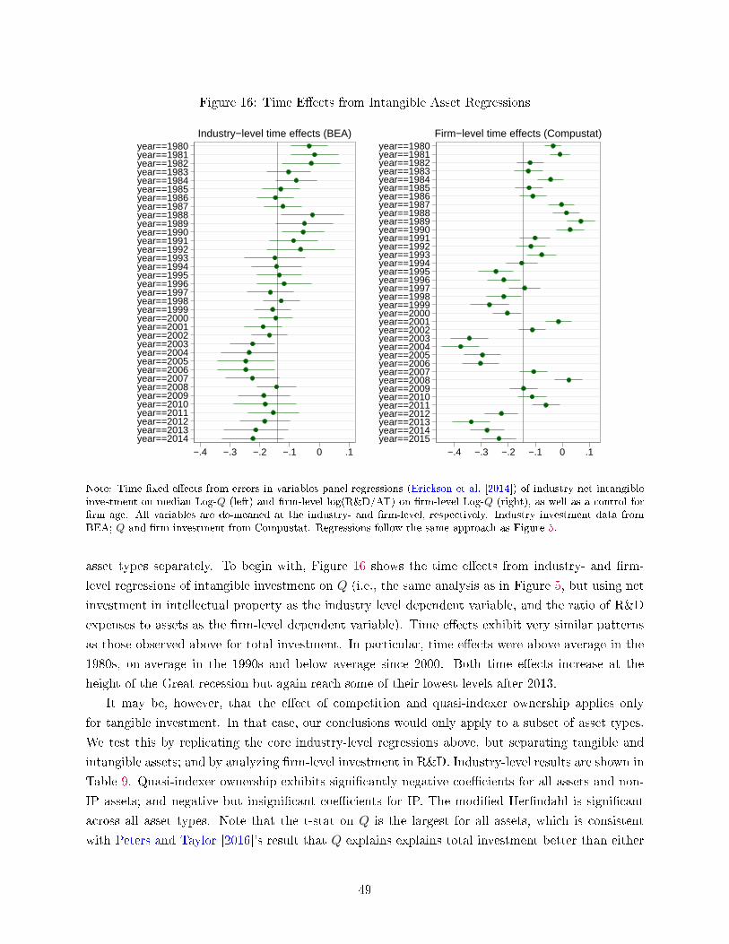
Figure 16: Time E�ects from Intangible Asset Regressions

year==1980year==1981year==1982year==1983year==1984year==1985year==1986year==1987year==1988year==1989year==1990year==1991year==1992year==1993year==1994year==1995year==1996year==1997year==1998year==1999year==2000year==2001year==2002year==2003year==2004year==2005year==2006year==2007year==2008year==2009year==2010year==2011year==2012year==2013year==2014

−.4 −.3 −.2 −.1 0 .1

Industry−level time effects (BEA)year==1980year==1981year==1982year==1983year==1984year==1985year==1986year==1987year==1988year==1989year==1990year==1991year==1992year==1993year==1994year==1995year==1996year==1997year==1998year==1999year==2000year==2001year==2002year==2003year==2004year==2005year==2006year==2007year==2008year==2009year==2010year==2011year==2012year==2013year==2014year==2015

−.4 −.3 −.2 −.1 0 .1

Firm−level time effects (Compustat)

Note: Time �xed e�ects from errors-in-variables panel regressions (Erickson et al. [2014]) of industry net intangibleinvestment on median Log-Q (left) and �rm-level log(R&D/AT) on �rm-level Log-Q (right), as well as a control for�rm age. All variables are de-meaned at the industry- and �rm-level, respectively. Industry investment data fromBEA; Q and �rm investment from Compustat. Regressions follow the same approach as Figure 5.

asset types separately. To begin with, Figure 16 shows the time e�ects from industry- and �rm-

level regressions of intangible investment on Q (i.e., the same analysis as in Figure 5, but using net

investment in intellectual property as the industry level dependent variable, and the ratio of R&D

expenses to assets as the �rm-level dependent variable). Time e�ects exhibit very similar patterns

as those observed above for total investment. In particular, time e�ects were above average in the

1980s, on-average in the 1990s and below average since 2000. Both time e�ects increase at the

height of the Great recession but again reach some of their lowest levels after 2013.

It may be, however, that the e�ect of competition and quasi-indexer ownership applies only

for tangible investment. In that case, our conclusions would only apply to a subset of asset types.

We test this by replicating the core industry-level regressions above, but separating tangible and

intangible assets; and by analyzing �rm-level investment in R&D. Industry-level results are shown in

Table 9. Quasi-indexer ownership exhibits signi�cantly negative coe�cients for all assets and non-

IP assets; and negative but insigni�cant coe�cients for IP. The modi�ed Her�ndahl is signi�cant

across all asset types. Note that the t-stat on Q is the largest for all assets, which is consistent

with Peters and Taylor [2016]'s result that Q explains explains total investment better than either

49

Table 9: Industry regressions, by asset typeTable shows the results of industry errors-in-variables panel regressions of Net I/K since 1990, split by asset type. All variablesare de-meaned at industry level over the regression period (i.e., we apply a `within' transformation). NI/K from BEA; remainingvariables primarily from Compustat. Annual data. T-stats in brackets. + p<0.10, * p<0.05, ** p<.01.

(1) (2) (3)

Net I/K

Mean All �xed

assets1+2Excluding

IP1IP2

Median Log-Q (t-1) 0.163** 0.190** 0.166+

[16.812] [7.870] [1.940]

Mean % QIX own (t-1) -0.118** -0.114** -0.368

[-3.068] [-2.869] [-1.340]

Mod-Her�ndahl (t-1) -0.056* -0.083** -0.143+

[-2.394] [-2.950] [-1.754]

Observations 1,110 1,110 1,109

Age controls YES YES YES

Year FE YES YES YES

Industry de-meaned YES YES YES

ρ2 0.39 0.427 0.194

physical or intangible investment separately. Firm-level results are shown in Table 7 above. As

shown, increased concentration and quasi-indexer ownership leads to under-investment in R&D.

We conclude that intangible assets are potentially more di�cult to accumulate. However, the

most striking result is that Q-theory works best when we combine tangible and intangible invest-

ment, suggesting that they are complementarily and jointly accumulated. Moreover, our results on

the role of competition and governance apply to both types of assets.

5.2.3 Missing Intangibles

Denote net investments in tangible and intangible assets by NIT and NII , such that total invest-

ments are NI = NIT + NII . Assume that tangible capital is perfectly measured but intangible

capital is under-estimated by a factor α � that is, assume that intangible investment is consistently

under-estimated across all industries. This is a simplifying assumption, but it highlights the main

reason for concern. Under this assumption, measured investment is given by

N̂I ≡ N̂IT + N̂II

(17)

= NIT + αNII (18)

The under-estimation of investment leads to under-estimation of capital K̂ and, since Q̂ is the ratio

of market value to replacement cost of capital, it leads to over-estimation of Q. Thus, a regression

of the form

50

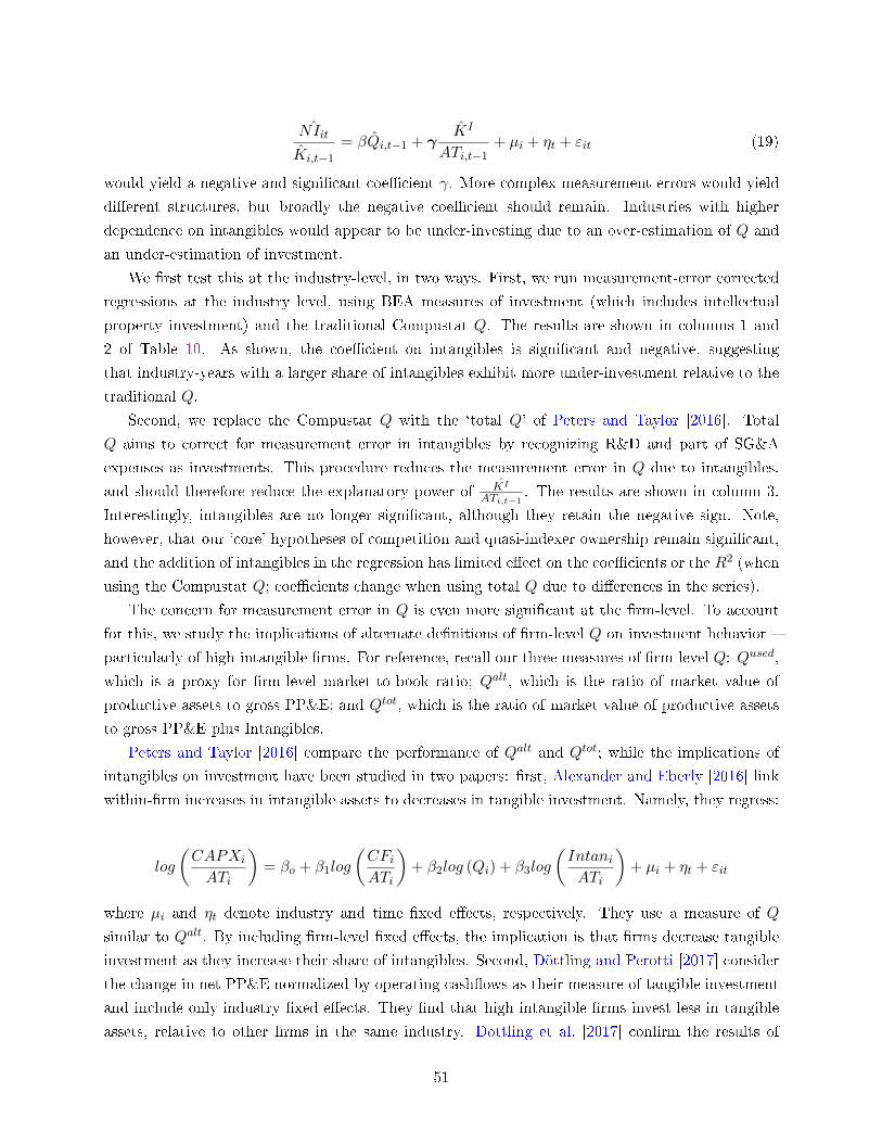
ˆNIit

K̂i,t−1= βQ̂i,t−1 + γ

K̂I

ATi,t−1+ µi + ηt + εit (19)

would yield a negative and signi�cant coe�cient γ. More complex measurement errors would yield

di�erent structures, but broadly the negative coe�cient should remain. Industries with higher

dependence on intangibles would appear to be under-investing due to an over-estimation of Q and

an under-estimation of investment.

We �rst test this at the industry-level, in two ways. First, we run measurement-error corrected

regressions at the industry level, using BEA measures of investment (which includes intellectual

property investment) and the traditional Compustat Q. The results are shown in columns 1 and

2 of Table 10. As shown, the coe�cient on intangibles is signi�cant and negative, suggesting

that industry-years with a larger share of intangibles exhibit more under-investment relative to the

traditional Q.

Second, we replace the Compustat Q with the `total Q' of Peters and Taylor [2016]. Total

Q aims to correct for measurement error in intangibles by recognizing R&D and part of SG&A

expenses as investments. This procedure reduces the measurement error in Q due to intangibles,

and should therefore reduce the explanatory power of K̂I

ATi,t−1. The results are shown in column 3.

Interestingly, intangibles are no longer signi�cant, although they retain the negative sign. Note,

however, that our `core' hypotheses of competition and quasi-indexer ownership remain signi�cant,

and the addition of intangibles in the regression has limited e�ect on the coe�cients or the R2 (when

using the Compustat Q; coe�cients change when using total Q due to di�erences in the series).

The concern for measurement error in Q is even more signi�cant at the �rm-level. To account

for this, we study the implications of alternate de�nitions of �rm-level Q on investment behavior �

particularly of high-intangible �rms. For reference, recall our three measures of �rm-level Q: Qused,

which is a proxy for �rm-level market-to-book ratio; Qalt, which is the ratio of market value of

productive assets to gross PP&E; and Qtot, which is the ratio of market value of productive assets

to gross PP&E plus Intangibles.

Peters and Taylor [2016] compare the performance of Qalt and Qtot; while the implications of

intangibles on investment have been studied in two papers: �rst, Alexander and Eberly [2016] link

within-�rm increases in intangible assets to decreases in tangible investment. Namely, they regress:

log

(CAPXi

ATi

)= βo + β1log

(CFiATi

)+ β2log (Qi) + β3log

(IntaniATi

)+ µi + ηt + εit

where µi and ηt denote industry and time �xed e�ects, respectively. They use a measure of Q

similar to Qalt. By including �rm-level �xed e�ects, the implication is that �rms decrease tangible

investment as they increase their share of intangibles. Second, Döttling and Perotti [2017] consider

the change in net PP&E normalized by operating cash�ows as their measure of tangible investment

and include only industry �xed e�ects. They �nd that high intangible �rms invest less in tangible

assets, relative to other �rms in the same industry. Dottling et al. [2017] con�rm the results of

51

Table 10: Industry regressions: Intangible Measurement ErrorTable shows the results of industry errors-in-variables panel regressions of Net I/K over the periods speci�ed. All variables are

de-meaned at industry-level. NI/K from BEA; remaining variables primarily from Compustat. Qtot from Peters and Taylor[2016], aims to correct for measurement error in intangibles. Annual data. T-stats in brackets. + p<0.10, * p<0.05, ** p<.01.

(1) (2) (3)

Net I/K

≥1990 ≥1990 ≥1990Median Log-Q (t-1) 0.163** 0.138**

[16.812] [23.700]

Median Log-Qtot (t-1) 0.138**

[20.330]

Mean % QIX own (t-1) -0.118** -0.110** -0.183**

[-3.068] [-3.015] [-3.231]

Mod-Her�ndahl (t-1) -0.056* -0.043* -0.075**

[-2.394] [-2.111] [-2.703]

Share of Intan Inv(t-1) -0.064* -0.015

[-2.298] [-0.295]

Observations 1,110 1,110 1,109

Age Controls YES YES YES

Year FE YES YES YES

Industry de-meaned YES YES YES

ρ2 0.39 0.387 0.545

Döttling and Perotti [2017] with a sample of European �rms.

Table 11 starts by comparing the empirical distribution (before winsorizing) of our three mea-

sures of Q over two periods: 1975-1980 and 2010-2015.39 As shown, all three distributions have

become increasingly skewed since 1980, but Qalt is by far the most a�ected: the 75th percentile

of the distribution as of 2010-2015 is 7.6, and the 90th percentile is 30. This is likely due to high

intangible �rms carrying low PP&E balances. Qtot resolves some of these issues by adding an es-

timate of intangible assets to the denominator, reaching a distribution similar to our proxy Qused.

Interestingly, the median Q also increased across all measures � especially Qalt and Qtot, which

increased by a factor of 8 and 4, respectively. Our measure, Qused, appears to be the most stable

of the three.

Such drastic di�erences in the distribution and skewness of Q have material implications for

regression results � particularly as they relate to the role of intangibles on investment; as well as

the e�ect of correcting for measurement error using the cumulant-estimator. Let us study these

implications.

Table 12 shows the results of regressing �rm-level net investment on Qused, Qalt and Qtot.

Columns 1-3 show OLS results with �rm �xed e�ects. Qused and Qtot exhibit strong statistical

signi�cance, especially compared to Qalt. Log-transforming all measures of Q substantially improves

the �t ofQalt, but has a limited e�ect onQused andQtot (in fact it decreases the �t forQtot). Columns

39We consider �rms after applying our data cleaning and exclusion criteria. In other words, our population includesonly US-incorporated �rms and excludes Utilities, Financials and Real Estate. See Section 3.3 for details.

52

Table 11: Percentiles of three measures of Q

1975-1980 2010-2015

Percentile Qused Qalt Qtot Qused Qalt Qtot

1% 0.5 -4.8 -1.0 0.5 -5.1 -0.9

5% 0.7 -1.5 -0.5 0.7 -0.6 -0.2

10% 0.7 -0.8 -0.3 0.9 0.0 0.0

25% 0.8 -0.2 -0.1 1.1 0.7 0.3

50% 1.0 0.3 0.2 1.6 2.1 0.8

75% 1.3 0.9 0.6 2.5 7.6 1.6

90% 1.9 2.5 1.4 4.4 30.0 3.4

95% 2.7 4.6 2.4 6.5 73.1 5.9

99% 6.6 24.1 9.6 16.2 746.2 22.4

1-3 also suggest that increases in intangible assets are correlated with decreases in net investment

within �rms. This conclusion, however, is sensitive to measurement error corrections: as shown in

columns 4-6, the coe�cient on intangible assets remains negative only for Qalt once controlling for

measurement error.40

This does not contradict our industry-level results, however. Column 7 and 8 shift from �rm to

industry �xed e�ects while using Qused and Qtot, respectively. As shown, we �nd a negative and

signi�cant coe�cient on intangible intensity � suggesting that high intangible �rms do invest less

in the cross-section. This is consistent with Dottling et al. [2017] and Döttling and Perotti [2017].

Industry-level investment may therefore decrease as high-intangible �rms account for a larger share

of the market. In unreported tests, we con�rm that out conclusions are robust to using CAPX/AT ,

instead of net investment as the dependent variable; as well as using the CRSP-Compustat Merged

sample instead of the full Compustat sample.

Our results lead to several conclusions. First, Qalt does not appear to be a valid proxy of Q

in the presence of high intangible �rms: either Qtot or Qused should be used going forward. Both

of these measures exhibit similar results and broadly similar levels of signi�cance. Second, Qused

appears like a reasonable, and stable proxy of Q.

5.2.4 Take-Away on Intangible Investment

The industry-level evidence suggests that high-intangible industries exhibit lower `measured' invest-

ment; and the �rm-level evidence suggests that high intangible �rms invest less in the cross section.

What portion of the under-investment can be explained by the rise of intangibles? We estimate

this by adding measures of intangible intensity to regressions similar to those underlying Figure

5. For industry results, we use the same regression as in Figure 5 and add the share of intangible

40We note that the positive coe�cient on Qtot is sensitive to log-transformations (i.e., it is negative and signi�cantwhen regressing net investment on log(Qtot)) but Qtot exhibits a much higher t-stat than log(Qtot). The positivecoe�cient on Qused remains even when using logs.

53

Table 12: Firm regressions: Intangible Measurement ErrorTable shows the results of �rm-level panel regressions of Net I/K against alternate measures of Q. Variables de-meaned at�rm- or industry-level, as noted. Total Q from Peters and Taylor [2016]; all remaining variables from Compustat.Annual data.T-stats in brackets. + p<0.10, * p<0.05, ** p<.01.

(1) (2) (3) (4) (5) (6) (7) (8)

Net CAPX/PPE

≥1980 ≥1980 ≥1980 ≥1980 ≥1980 ≥1980 ≥1980 ≥1980Qused (t-1) 0.074** 0.218** 0.103**

[84.810] [50.108] [50.807]

Qalt (t-1) 0.000** 0.000**

[6.238] [3.154]

Qtot (t-1) 0.076** 0.207** 0.098**

[105.324] [65.656] [71.389]

Intan/Assets(t-1) -0.048** -0.165** -0.035** 0.158** -0.103** 0.123** -0.028* -0.049**

[-4.145] [-13.804] [-3.113] [7.574] [-6.214] [5.724] [-2.338] [-4.103]

Observations 116,351 113,527 115,473 116,351 113,527 115,473 116,351 115,473

Method OLS EW EW

Age Controls YES YES YES

Year FE YES YES YES

Firm de-meaned YES YES NO

Industry de-meaned NO NO YES

ρ2 0.139 0.082 0.171 0.258 0.0747 0.33 0.205 0.246

investment as a predictor variable. For �rm-level results, we move from industry- to �rm-level �xed

e�ects (given the results in Table 10) and add the the �rm-level ratio of intangibles to assets to the

regression.

Figure 17 shows the results, where we have re-centered the �xed e�ects at zero and �ipped the

plot for readability. The rise of intangibles appears to explain a quarter to a third of the observed

investment gap. Importantly, adding intangibles not only increases the time e�ects after 2000 but

also decreases them before 1990 � suggesting that part of the long term drop in investment is in

fact driven by the rise of intangibles. Our estimate of the impact of intangibles is broadly consistent

with that of Alexander and Eberly [2016].

Even after controlling for intangible investment, however, large and persistent negative time

e�ects remain after 2000 � time e�ects that are correlated with increased concentration and increased

quasi-indexer ownership. Corporations have reduced investment in both tangible and intangible

assets since 2000, suggesting that other factors are in play. We conclude that the rise of intangibles

accounts for some � a quarter to a third � but not all of the observed under-investment.

5.3 Debt issuance and investment by highly-rated �rms

According to the safe asset scarcity hypothesis, the value of being able to issue safe assets increased

after the Great Recession. This should increase the value of very safe (AA to AAA) �rms, but, to

the extent that safety cannot be readily scaled up, it would not increase their physical investment to

54

Figure 17: Time E�ects from Intangible Asset Regressions

−.0

2−

.01

0.0

1.0

2.0

3

1980 1985 1990 1995 2000 2005 2010 2014

Only Q Q + Intan

Industry−level FE with and w/o intangibles−

.02

0.0

2.0

4

1980 1985 1990 1995 2000 2005 2010 2015

Only Q Q + Intan

Firm−level FE with and w/o intangibles

Note: Time �xed e�ects from errors-in-variables panel regressions (Erickson et al. [2014]) of industry net investmenton median Q (top) and (CAPX+R&D)/AT on �rm-level Q (bottom), as well as a control for �rm age. Industryregressions follow the same speci�cation as in Figure 5 (i.e., the green line corresponds to the same �xed e�ects asthose of Figure 5, except that they have been de-meaned here). Firm regressions based on de-meaned variables atindustry-level instead of �rm-level for the reasons discussed in the text. Industry investment data from BEA; Q and�rm investment from Compustat.

55

Table 13: Safe Asset Scarcity: Valuation testTable shows the results of �rm-level OLS regressions of Market Value, PP&E and Assets as of 2014 on 2006 Market value anda AA-to-AAA rating indicator. Annual data, sourced from Compustat. T-stats in brackets. + p<0.10, * p<0.05, ** p<.01.

(1) (2) (1) (2) (1) (2)

Log MV (2014) Log PPE (2014) Log Assets (2014)

AA to AAA rated (2006) -0.079 -0.241 -0.362 -0.224 -0.205 -0.274

[-0.34] [-1.03] [-0.94] [-0.65] [-0.98] [-1.31]

Log MV (2006) 0.036 0.021 0.192* 0.170* 0.032 0.034

[0.70] [0.40] [2.27] [2.22] [0.70] [0.73]

Log Assets (2006) 1.034** 1.001** 0.373** 0.459** 0.546** 0.552**

[25.75] [24.17] [5.60] [7.55] [15.27] [14.98]

Log(age) -0.008 0.03 0.748** 0.613** 0.455** 0.443**

[-0.20] [0.73] [11.36] [10.09] [12.90] [12.04]

Industry FE No Yes No Yes No Yes

Observations 1795 1795 1781 1781 1795 1795

Overall R2 0.85 0.858 0.721 0.793 0.873 0.879

the same extent that it increases their value. This might then account for relatively low investment

despite high Q. Note that, at some broad abstract level, this is an example of decreasing returns to

(physical) scale.

To better understand whether this hypothesis is supported by the data, this section discusses

valuation and investment patterns of AA to AAA rated �rms and below AA-rated �rms. To mitigate

endogeneity problems, we assign �rms to rating groups based on their 2006 rating, before the Great

Recession. The year 2006 is chosen because safe asset scarcity is understood to be a post-Great

Recession e�ect.

We start with valuations. According to the safe asset scarcity hypothesis, the value of being able

to issue safe assets increased after the Great Recession. In that case, valuation (and investment, to

a lesser extent) of highly rated �rms should increase relative to that of other �rms.We regress the

2014 value on the 2006 value and an indicator for AA to AAA rated �rms:

logMVi,2016 = β0 + β1log agei + β2log assetsi,2006 + log MVi,2006 + I{AA−AAAi,2006}+ εi (20)

We include industry �xed e�ects in some regressions; and run a similar regression for capital (PP&E)

and assets to test for higher (cumulative) capital expenditures or balance sheet growth. Table 13

summarizes the results. As shown, the coe�cient on the AA to AAA rated indicator is not signi�cant

and, if anything, it is negative. In unreported tests, we �nd positive results at the height of the

Great Recession (2009 and 2010), but not in later years. The AAA premium did exist immediately

after the Great Recession, but it was short lived, and cannot account for valuation and investment

after 2010.

Let us move on to investment patterns. Figure 18 shows the average log-change in total assets

56

Figure 18: Assets and investment, by rating

−.0

50

.05

.1.1

5.2

1970 1975 1980 1985 1990 1995 2000 2005 2010 2015year

A and below AA to AAA

Average Log−change in Total Assets

.06

.08

.1.1

2.1

4.1

6

1970 1975 1980 1985 1990 1995 2000 2005 2010 2015year

A and below AA to AAA

Average NI/K, inc R&D

Note: Annual data. Firms mapped to categories based on ratings as of 2006.

and the average net investment rate (including R&D expenses) for both groups of �rms.41 At least

until 2012, both groups of �rms seem to be increasing assets at roughly the same rate. By contrast,

the investment rate of highly rated �rms has been well-below that of lower rated �rms since 1990.

This suggests that highly rated �rms have grown their balance sheets at roughly the same rate as

lower-rated �rms, but have invested less.

Have these �rms reduced external �nancing given the lower investment? To answer this question,

we follow Frank and Goyal [2003] and compute the uses and sources of funding based on Compustat

data. Speci�cally, we de�ne the total �nance de�cit as the sum of dividends, investment and changes

41Conclusions are qualitatively similar excluding R&D expenses from the NI/K calculation

57

in working capital minus internal cash �ow:42

DEF = DIV + INV + ∆WC − IntCF (21)

Note that this de�nition of investment is substantially broader than capital expenditures: it includes

all short and long term investment as de�ned in the statement of cash �ows. We also compute net

debt and equity issuance, such that DEF = NetDebtIss+NetEqIss.

Figure 19 shows the 2-year cumulative �nancing de�cit, debt and equity issuance by rating group,

normalized by total assets. We highlight the year 1982, when SEC Rule 10b-18 was instituted,

which allows companies to repurchase their shares on the open market without regulatory limits.

Two interesting conclusions arise: �rst, both types of �rms have either maintained or increased their

debt issuance since the mid-1990s. Highly rated �rms issued a substantial amount of debt in 2009,

at the height of the Great Recession. Such debt issuance allowed them to maintain large buybacks

despite lower internal funds. They decreased issuance in the early 2010s but returned to the market

in 2015 as internal funds decreased but buybacks remained high. Low rated �rms issued almost

no debt during the Great Recession, which led to a substantial decrease in buybacks. But they

quickly returned to the market after the crisis, and used the funds raised primarily for buybacks.

Second, buybacks at highly-rated �rms increased soon after 1982, moving almost one-to-one with

the internal �nance de�cit for the past 20 years. The increase in buybacks is much less pronounced

for lower rated �rms until the mid-2000s. In fact, lower rated �rms maintained a positive �nance

de�cit until about 2000, which was �nanced primarily with debt.

42The following Compustat items are used: Div = div, INV = capx + ivch + aqc− sppe− siv − ivstch− ivaco,∆WC = −recch− invch− apalch− txach− aoloch+ chech− fiao− dlcch and IntCF = ibc+ xidoc+ dpc+ txdc+esubc + sppiv + fopo + exre. Note that adjusted de�nitions are used for prior disclosure regimes � see Frank andGoyal [2003] for additional details.

58

Figure 19: Uses and sources of �nancing, by rating

−.0

50

.05

1970 1980 1990 2000 2010 1970 1980 1990 2000 2010

A and below AA to AAA

Financing deficit Debt IssuanceEquity Issuance

year

Note: 2-year cumulative rates, normalized by total assets. Based on annual data. Firms mapped to categories basedon ratings as of 2006. The vertical line on 1982 highlights the passing of SEC rule 10b-18, which allows companiesto repurchase their shares on the open market without regulatory limits.

The improving �nance de�cit and associated buybacks may be driven by increasing pro�ts, or

by decreasing investments. Table 14 decomposes the sources and uses of �nancing for highly rated

�rms and lower-rated �rms. As shown, the improving �nance de�cit for both types of �rms is driven

by decreasing investments and, to a lesser extent, working capital. Cash dividends have remained

stable while cash �ow decreased slightly. The decrease in investment is particularly pronounced for

highly rated �rms, from ∼11% in the 1970s and 1980s to only 6% in the 2000s.

6 Interpretation of Macro-economic Trends

Recent work in the macro-literature has studied the slow U.S. recovery following the Great Recession.

Fernald et al. [2017] (FHSW), in particular, use a quantitative growth-accounting decomposition to

study the output shortfall. According to their calculations, the shortfall is almost entirely explained

by slower TFP growth and decreased labor force participation. Focusing on the capital stock, they

argue that �although capital formation has been below par [since 2009], so has output growth, and

by 2016, the capital/output ratio was in line with its long-term trend.�

Our goal in this section is to test how the growth accounting decomposition of Fernald et al.

59

Table14:Funds�ow

and�nancingas

afraction

oftotalassets,byrating(%

)

Rating

Field

/Year

1970-1979

1980-1989

1990-1994

1995-1999

2000-2004

2005-2009

2010-2015

AAto

AAA

rated�rm

s

Cash

dividendsa

3.7

3.9

4.3

4.7

4.5

4.2

4

Investm

entsb

9.7

11.9

8.4

7.9

7.3

6.2

6.2

∆Workingcapitalc

1.6

-0.3

0.5

1.4

1.4

0.8

0.1

Internalcash

�ow

d14.2

15.8

13.8

15.6

16.3

15.7

13

Financingde�cita+b+c-d

0.7

0.1

-0.7

-1.9

-2.7

-3-2.3

Net

debtissues

10.6

0.2

0.4

0.3

0.4

1.1

0.6

Net

equityissues

20.1

-0.1

-1.1

-2.2

-3.1

-4.1

-2.9

Netexternal�nancing1+2

0.7

0.1

-0.7

-1.9

-2.7

-3-2.3

BelowAA

rated�rm

s

Cash

dividendsa

2.6

2.5

2.1

1.8

1.3

1.7

2

Investm

entsb

10.7

12.2

7.8

9.3

6.8

7.4

7.8

∆Workingcapitalc

1.8

0.9

0.8

21.9

1.5

1.4

Internalcash

�ow

d13.4

14

10.1

11.7

9.8

11.3

11.7

Financingde�cita+b+c-d

1.5

1.1

0.4

10.2

-0.7

-0.6

Net

debtissues1

1.2

1.1

0.2

1.6

0.6

1.3

1.7

Net

equityissues

20.3

00.2

-0.7

-0.4

-2.1

-2.4

Netexternal�nancing1+2

1.5

1.1

0.4

0.9

0.2

-0.8

-0.7

Notes:Annualdata,in

percentages.Basedontheaverageofyearlycumulativetotalsacrossall�rm

sin

each

category.Firmsmapped

tocategories

basedon2006

ratings.

60

[2017] would deal with an increase in markups. To tease out the e�ect of increased market power

on growth-accounting decompositions, we generate 100 simulations of an economy under increasing

mark-ups using the model in Jones and Philippon [2016], which is brie�y described in the Appendix.

We assume a change in the steady-state markup from 20% to 35% over 100 quarters.43 We use

the simulations to study the contribution of alternate macro-series to aggregate output under the

following two decompositions (see FHSW for their derivation):

∆log(Yt) = ∆log(TFPt) + αt∆log(Kt) + (1− αt)∆log(Nt) (22)

and

∆log(Yt) =∆log(TFPt)

1− αt+

αt1− αt

∆log

(Kt

Yt

)+ ∆log(LQt) (23)

where αt denotes the capital share of output and LQt denotes labor quality. We model only total

labor Nt, so in our simulated data ∆log(LQt) = 0. All other de�nitions are standard.

Each simulation includes estimates for the growth of output, consumption, labor and capital; as

well as shocks to economy-wide TFP (among others). Using the simulated series, we estimate each

of the components in equations 22 and 23. We report results using the change in measured TFP ,

de�ned as

∆log(TFPt) =∆log(Yt)− αtlog(Kt)− (1− αt)∆log(Nt) [−αtlog(Kt−1)] (24)

where αt = αt+αt−1

2 .44 This de�nition roughly follows Fernald [2014] (which is used in FHSW), but

two items are worth highlighting: �rst, Fernald [2014] carefully controls for changes in utilization

when computing TFP. This issue is moot in the simulated data because our model does not include

variable utilization. Second, Fernald [2014] maintains the assumption of zero pro�ts. He estimates

the factor shares using BLS output data excluding taxes. This approach implies that any pro�t

above and beyond the rental cost of capital is included in the capital share. To mirror this approach,

we re-estimate αt every period as WtNtYt

.45

43This is comparable in size to the estimate in Jones and Philippon [2016]. The model is calibrated and theshocks estimated using a Kalman-Filter, taking into account the Zero Lower Bound on nominal rates. See Jones andPhilippon [2016] for the details of the model.

44We use the average capital share across adjacent periods rather than the the time t capital share to (roughly)account for the increase in the capital share with market power. This is the standard approach, but note that it canbe substantially biased in periods of rising capital shares as simulated here (and observed in recent years). In fact,the change in measured TFP could be written as:

∆log(TFPt) =∆log(Yt)− [αtlog(Kt)− (αt −∆αt)log(Kt−1)]− [(1− α)log(Nt)− (1− (αt −∆αt))log(Nt−1)] (25)

=∆log(Yt)− αt∆log(Kt)− (1− αt)∆log(Nt)−∆αt

[log

(Kt−1

Nt

)]where the last term captures changes in capital shares, and can be material for large cumulative changes in capitalshares.

45Estimating labor shares based on the Cobb-Douglas production structure yields similar results. Namely, for agiven elasticity of substitution εt, the implied mark-up is µt = εt

1−εt and the corresponding labor share is sNt = 1−αµt

.

61

Armed with our time series of changes, we then follow FHSW to decompose the simulated series

into a cyclical, trend and residual (i.e., irregular) components (ct, µt and zt, respectively):

yt = ct + µt + zt (26)

The only di�erence between our decomposition and that of FHSW is that we use employment as

our basis for Okun's law instead of unemployment [Okun, 1962]. The decomposition proceeds as

follows. First, ct is estimated using a Generalized Okun's law

ct =

q∑j=−p

βj∆nt+j = β(L)∆nt (27)

where we use total labor n as our basis for calculations. βj is estimated through a simple OLS

regression with two forward and backward lags (p = q = 2). Substituting equation 27 into 26, we

obtain the Okun's Law residual (which includes the long-run trend µt)

yt − β(L)∆nt = µt + zt (28)

The second term, β(L)∆nt, captures the change in a given time series yt that can be explained by

changes in employment. Next, we estimate µt as a long-run smoothed value of y after removing the

cyclical part. Namely

µ̂t = κ(L)(yt − β̂(L)∆nt

)(29)

where κ(L) is a biweight �lter with truncation parameter of 60. Note that this trend-cycle-irregular

decomposition preserves additivity.

The basic results are shown in Table 15, along with the results of FHSW for comparison.

Columns 1 and 2 show the median and standard deviation across 100 simulations of the Gener-

alized Okun's law coe�cient β(1). Row 1 shows that an increase in employment of 1 percent leads

to an increase in output of 0.68 percent � as expected given the use of α = 0.33. The increase is

explained by a mixture of TFP and labor Nt (rows a and c). Similarly, row 2 shows that output-

per-unit of labor decreases by 0.32 percent when employment increases by 1 percent. This is driven

by a drop in K/Y partly compensated by a rise in TFP (rows d and e). The behavior of K/Y is rel-

evant. FHSW note that, in theory, slower TFP growth should raise the steady-state capital/output

ratio � but this is not what the data show. The capital/output ratio has been fairly smooth since

the 1970s. In the benchmark model, the channel from TFP growth to K/Y is via the interest rate

and the cost of capital. Lower trend-growth leads to a lower interest rate, which lowers the cost

of capital and increases K/Y. We have indeed observed a decrease in the real interest rate and in

the cost of funds, but it did not seem to translate into a clear increase in K/Y. The lack of growth

in the capital/output ratio may therefore be driven by other factors, such as an increase in market

power or the rise of superstar �rms.

The `measured' capital share of output including pro�ts is then α̂t = 1− 1−αµt

62

Figure 20: Standard deviation of Trend-Residual Gap in K/Y , by simulation period

0 10 20 30 40 50 60 70 80 90 1000.006

0.008

0.01

0.012

0.014

0.016

0.018

0.02

0.022

0.024

In order to compare coe�cients to those of FHSW, �rst recall that we use employment and

they use unemployment as the basis for Okun's law, so we �ip the signs of their estimates to make

the comparison easier. The volatility of log changes in employment and unemployment are not the

same, which might explain the di�erences in magnitudes as well. Also note that FHSW consider

output per capita under the �rst decomposition, vs. total output (with �xed population) in our

case. Nonetheless, we �nd common patterns in terms of the relative contribution and volatility of

the coe�cients. Our trend component is much less volatile than that of FHSW, as expected since

we simulated de-trended series except for the rise in market power. Of the remaining series, some

of our components appear less volatile (e.g., irregular components) but they are almost always in

the same order of magnitude.

Columns (6) and (7) show our primary measure of interest: the median and standard deviation

of cumulative gaps between cycle-adjusted and long-run trends for each measure. As shown, cycle

adjusted quantities are largely captured by the trend decomposition: median gaps are essentially

zero, and the corresponding standard deviations are also quite small. Thus, it appears that the

cycle-trend-irregular decomposition of Fernald et al. [2017] absorbs the rise in market power. The

decomposition does not seem able to separately identify deviations from trend in K/Y driven by

(long term) changes in market power.

It is also worth noting that the residual and trend series approach each other towards the end of

the sample by construction. Figure 20 shows the standard deviation of the gap between the trend

and residual K/Y series by simulation period. As shown, the standard deviation decreases rapidly

as you approach the end of the series. This e�ect appears for virtually all simulated quantities �

likely due to the additional weight placed on observations when using a truncated bi-weight �lter.

To further study the dynamics, Figure 21 and 22 show the cumulative changes in output, `mea-

sured' TFP, capital, labor, output-labor ratio and capital-output ratio; for a simulation with no

shocks (except the rise in market power) and with shocks, respectively. For each series, we include

63

Table15:Macro-estimates

Table

show

sthemedianandstandard

deviationoftheresultsacross

allsimulatedseries

withstochastic

shocks,against

thecoe�

cients

inFHSW.Recallthat

FHSW

use

unem

ploymentasthebasisofOkun'slawandweuse

employment,hence

coe�

cientsare

�ipped.Wereportcoe�

cientβ

(1)(β

(1)/

4in

FHSW),which

measure

per-periodincreasesin

outputrelativeto

apercentagepointchangein

theem

ployment(unem

ployment)rate.Thestandard

deviationsofthecomponents

are

forquarterly

growth

ratesreported

inpercentagepoints

atanannualrate.R

2reported

only

forGP'sregressionofeach

variable

onem

ployment(FHSW

reportR

2forregressiononfactors,whichfollow

sadi�erentmethod).

Note

thatsub-components

may

notaddupperfectly

aswereport

themediansacross

simulations.

(1)

(2)

(3)

(4)

(5)

(6)

(7)

(8)

(9)

(10)

(11)

(12)

(13)

GeneralizedOkun'slawcoe�.

Std.deviationofcomponents

MedianR

2

from

Okun'slaw

regression

Gapto

trend

att

=100

GP

FHSW‡

GP:Sim

.Median

FHSW:Actual

Median

St.

Dev.

Coe�

St.

Dev.

cycle

(c)

trend

(µ)

irregular

(z)

cycle

(c)

trend

(µ)

irregular

(z)

Median

St.

Dev.

1.Ya+b+c

0.68

0.08

2.02

0.20

1.19

0.08

1.22

2.51

0.54

2.12

0.48

0.00

0.01

a.TFP

0.09

0.08

0.5

0.19

0.32

0.08

1.20

1.24

0.24

2.27

0.06

0.00

0.01

b.αKt

0.01

0.01

0.09

0.06

0.03

0.06

0.13

0.2

0.19

0.32

0.04

0.00

0.01

c.(1−α

)Nt

0.58

0.01

1.43

0.14

0.97

0.00

0.04

1.54

0.26

1.24

1.00

0.00

0.00

2.Yt/N

d+e+f

t-0.32

0.08

-0.28

0.22

0.61

0.08

1.22

0.77

0.37

2.23

0.20

0.00

0.01

d.TFP/(1−α

)0.16

0.14

0.75

0.29

0.54

0.13

2.09

1.88

0.35

3.41

0.06

0.00

0.02

e.K/Y×α/(1−α

)-0.48

0.06

-0.90

0.09

0.84

0.09

0.90

1.3

0.07

1.09

0.46

0.00

0.01

f.LaborQuality

NA

NA

-0.13

0.05

NA

NA

NA

0.37

0.05

0.99

NA

NA

NA

‡FHSW

coe�

cientsigns�ipped

given

theiruse

ofunem

ploymentforOkun'slaw(vs.

employmentusedhere).Alsonote

thatdecomposition1isbasedonoutputper

capital

inFHSW,vs.totaloutput(witha�xed

population)in

ourcase.

64

Figure 21: Sample simulations: Cumulative changes with only market power

0 20 40 60 80 100-0.08

-0.06

-0.04

-0.02

0

0.02y

0 20 40 60 80 100-4

-3

-2

-1

0

110-3 tfp

0 20 40 60 80 100-0.12

-0.1

-0.08

-0.06

-0.04

-0.02

0

0.02k

0 20 40 60 80 100-0.04

-0.03

-0.02

-0.01

0n

0 20 40 60 80 100-0.04

-0.03

-0.02

-0.01

0

0.01yn

0 20 40 60 80 100-0.04

-0.03

-0.02

-0.01

0

0.01ky

RawResidualTrend

Note: Blue series shows the cumulative raw changes; red series shows the employment-adjusted series; and yellowseries shows the long-run trend. We assume a change in the steady-state markup from 20% to 35% over 100 quarters.

the raw, cyclically adjusted and trend series. Several items are worth highlighting.

First, as shown in Figure 21 (i.e., the simulation without shocks), the rise of market-power

pushes output, capital and labor productivity down. Measured TFP goes down a little, but the

magnitude of the decline is very small.

Looking at the cycle- and trend-adjusted series we see that the entire decrease is captured

by Okun's law decomposition: both the residual and trend are essentially zero. This is because

employment moves with market power, along with all the other series. So employment can `explain'

all of the trends even though the only parameter a�ecting the simulated economy is the level of the

markup.

Moving to Figure 22, which adds stochastic shocks, we �nd substantial additional variation in

the trends. Importantly, the decrease in employment driven by the rise of market power accounts

for a large part of the decreases in all series: the cycle- and trend-adjusted series are much closer to

zero than the actuals. This is particularly true for the K/Y series, which remains largely around

zero over the full period (this is fairly consistent across all simulations). The actual series, however,

drops well-below trend as observed in the data (this is true in some, not all simulations obviously).

Focusing on the period with the largest output drop (around the 40-60th simulation period),

the reduction in output leads to an increase in capital-output ratio relative to trend, and a decrease

in `measured' TFP relative to trend. This is in-line with the results in Fernald et al. [2017] who

allocate the output shortfall to lower TFP while noting that K/Y remains in line with trend.

Importantly, these patterns are consistent across simulations: de�ne the crisis trough as the last

period in a given simulation that exhibits a cumulative drop of output greater than 8% over ten or

65

Figure 22: Sample simulation: Cumulative changes with shocks

0 20 40 60 80 100-0.2

-0.15

-0.1

-0.05

0

0.05

0.1

0.15y

0 20 40 60 80 100-0.04

-0.02

0

0.02

0.04

0.06

0.08tfp

0 20 40 60 80 100-0.4

-0.3

-0.2

-0.1

0

0.1k

0 20 40 60 80 100-0.05

-0.04

-0.03

-0.02

-0.01

0

0.01

0.02n

0 20 40 60 80 100-0.15

-0.1

-0.05

0

0.05

0.1

0.15yn

0 20 40 60 80 100-0.2

-0.15

-0.1

-0.05

0

0.05ky

RawResidualTrend

Note: Blue series shows the cumulative raw changes. Red series shows the employment-adjusted series. Yellow seriesshows the long-run trend.

fewer periods; and the post-crisis period as the (at most) 28 quarters following the trough. Then

compute the average quarterly gap between the (cumulative) cycle-adjusted and trend series for

TFP and K/Y over the post-crisis period in each simulation. This gives an estimate of the gap to

trend following a crisis under rising mark-ups. The median average gap to trend in TFP is -0.35%,

while the median gap for K/Y is +0.13% (i.e., TFP is below trend while K/Y is above trend).

29% of the average simulation gaps are positive for TFP compared to 71% for K/Y . these results

suggest that (even) in the presence of rising mark-ups, the output gap following a crisis can appear

to be in TFP rather than K/Y � consistent with the �ndings of Fernald et al. [2017].

Overall, we conclude that growth-accounting decompositions may confound a rise in market

power with a decrease in TFP , and conclude that any output gaps are due to lower TFP rather

than market power.

7 Conclusion

Private �xed investment in the United States has been lower than expected since the early 2000's.

The trend started before 2008, but the Great Recession made it more striking. Investment is low

despite high levels of pro�tability and Tobin's Q. This simple observation rules out a whole class

of theories that would explain low investment along with low values of Tobin's Q, and guides us to

theories that predict low investment despite high Q. We test 8 such theories, and �nd consistent

support for decreased competition, tightened governance/increased short-termism and intangibles

in our industry and �rm level datasets. The rise of intangibles explains a quarter to a third of the

66

investment gap, yet it leaves large and persistent residuals after 2000. These residuals are explained

by decreased competition and tightened governance/increased short-termism. These conclusions

are based on simple regressions and therefore cannot establish causality between competition, gov-

ernance and investment. We address this in follow-up work by relying on a combination of instru-

mental variables and natural experiments [Gutiérrez and Philippon, 2017a,b]. Last, we show that

standard growth-accounting decompositions may be unable to separately identify deviations from

trend in K/Y driven by (long term) changes in market power. As a result, such decompositions

may confound a rise in market power with a decrease in TFP , and conclude that any declines in

output are due to lower TFP rather than higher market power.

If our conclusions are correct, they suggest that U.S. policy makers should focus on increasing

competition in the market for goods and services. Related research [Grullon et al., 2016, Dottling

et al., 2017] suggests a role for reducing barriers to entry and product market regulations, as well

as improving anti-trust enforcement.

References

Andrew B. Abel and Janice C. Eberly. A uni�ed model of investment under uncertainty. The

American Economic Review, 84(5):1369�1384, 1994. ISSN 00028282. URL http://www.jstor.

org/stable/2117777.

Andrew B. Abel and Janice C. Eberly. Investment, valuation, and growth options. Working Paper,

Wharton, 2005.

Viral Acharya and Guillaume Plantin. Monetary easing and �nancial instability. 2016.

Philippe Aghion, John Van Reenen, and Luigi Zingales. Innovation and institutional ownership.

American Economic Review, 103(1):277�304, February 2013. doi: 10.1257/aer.103.1.277. URL

http://www.aeaweb.org/articles?id=10.1257/aer.103.1.277.

Philippe Aghion, Stefan Bechtold, Lea Cassar, , and Holger Herz. The causal e�ects of competition

on innovation: Experimental evidence. NBER Working Paper, 2014.

Omar Al-Ubaydli and Patrick A. McLaughlin. Regdata: A numerical database on industry-speci�c

regulations for all united states industries and federal regulations, 1997 to 2012. Regulation &

Governance, 2015.

Lewis Alexander and Janice Eberly. Investment hollowing out. Working Paper, 2016.

Laura Alfaro, Thorsten Beck, and Charles Calomiris. Foreign bank entry and entrepreneurship.

Working Paper, 2015.

Heitor Almeida, Vyacheslav Fos, and Mathias Kronlund. The real e�ects of share repurchases.

Journal of Financial Economics, 119(1):168�185, 2016.

67

Ian R. Appel, Todd A. Gormley, and Donald B. Keim. Passive investors, not passive owners. Journal

of Financial Economics, 121(1):111 � 141, 2016a.

Ian R. Appel, Todd A. Gormley, and Donald B. Keim. Standing on the shoulders of giants: The

e�ect of passive investors on activism. Working Paper 22707, National Bureau of Economic

Research, September 2016b.

John Asker, Joan Farre-Mensa, and Alexander Ljungqvist. Corporate investment and stock market

listing: A puzzle? Review of Financial Studies, 2014.

David Autor, David Dorn, Lawrence Katz, Christina Patterson, and John Van Reenen. Concen-

trating on the fall of the labor share. Technical report, mimeo, jan 2017a.

David Autor, David Dorn, Lawrence F. Katz, Christina Patterson, and John Van Reenen. The

fall of the labor share and the rise of superstar �rms. Working Paper 23396, National Bureau of

Economic Research, May 2017b. URL http://www.nber.org/papers/w23396.

Jose Azar, Sahil Raina, and Martin C. Schmalz. Ultimate ownership and bank competition. Working

paper, 2016a.

Jose Azar, Martin C. Schmalz, and Isabel Tecu. Anti-competitive e�ects of common ownership.

Working paper, 2016b.

Rudiger Bachmann, Ricardo J. Caballero, and Eduardo M. R. A. Engel. Aggregate implications

of lumpy investment: New evidence and a dsge model. American Economic Journal: Macroe-

conomics, 5(4):29�67, October 2013. doi: 10.1257/mac.5.4.29. URL http://www.aeaweb.org/

articles?id=10.1257/mac.5.4.29.

Simcha Barkai. Declining labor and capital shares. University of Chicago, 2017.

Jan Bena, Miguel A. Ferreira, Pedro P. Matos, and Pedro Pires. Are foreign investors locusts?

the long-term e�ects of foreign institutional ownership. European Corporate Governance Institute

(ECGI) - Finance Working Paper No. 468/2016, 2016.

Ben Bernanke and Mark Gertler. Agency costs, net worth and business �uctuations. American

Economic Review, 79:14�31, 1989.

Ben S. Bernanke. Irreversibility, uncertainty, and cyclical investment. The Quarterly Journal of

Economics, 98(1):85�106, 1983.

James E. Bessen. Accounting for rising corporate pro�ts: Intangibles or regulatory rents? Boston

Univ. School of Law, Law and Economics Research Paper No. 16-18, 2016.

Bruce A. Blonigen and Justin R. Pierce. Evidence for the e�ects of mergers on market power and

e�ciency. Working Paper 22750, National Bureau of Economic Research, October 2016.

68

William C. Brainard and James Tobin. Pitfalls in �nancial model-building. The American Economic

Review, (244), 1968. URL http://EconPapers.repec.org/RePEc:cwl:cwldpp:244.

Andra Buca and Philip Vermeulen. Corporate investment and bank-dependent borrowers during

the recent �nancial crisis. Technical report, ECB Working Paper 1859, 2015.

Brian J. Bushee. The in�uence of institutional investors on myopic r&d investment behavior. The

Accounting Review, 73(3):305�333, 1998.

Brian J. Bushee. Do institutional investors prefer near-term earnings over long-run value? Con-

temporary Accounting Research, 18(2):207�246, 2001.

M. Bussiere, L. Ferrara, and J. Milovich. Explaining the Recent Slump in Investment: the Role

of Expected Demand and Uncertainty. Working papers 571, Banque de France, 2015. URL

https://ideas.repec.org/p/bfr/banfra/571.html.

Ricardo Caballero. Aggregate investment. In John B. Taylor and Michael Woodford, editors,

Handbook of Macroeconomics, volume 1B, Amsterdam, 1999. Elsevier Science, North Holland.

Ricardo Caballero and Eduardo Engle. Explaining investment dynamics in u.s. manufacturing: A

generalized (s,s) approach. Econometrica, 67:783�826, 1999.

Ricardo J. Caballero and Emmanuel Farhi. The safety trap. NBER Working Papers 19927, National

Bureau of Economic Research, Inc, February 2014.

CEA. Bene�ts of competition and indicators of market power. Issue Brief, April 2016.

Yen-Cheng Chang, Harrison Hong, and Inessa Liskovich. Regression discontinuity and the price

e�ects of stock market indexing. Review of Financial Studies, 2014.

Brian Chen, Samuel G. Hanson, and Jeremy C. Stein. The decline in big-bank lending to small

businesses: Causes and consequences. Working paper, 2016.

Alan D. Crane, Sebastien Michenaud, and James P. Weston. The e�ect of institutional ownership

on payout policy: Evidence from index thresholds. Review of Financial Studies, 2016.

Jason G. Cumins, Kevin A. Hasset, and Stephen D. Oliner. Investment behavior, observable expec-

tations, and internal funds. American Economic Review, 96(3):796�810, 2006.

Steven Davis, John Haltiwanger, Ron Jarmin, and Javier Miranda. Volatility and dispersion in

business growth rates: Publicly traded versus privately held �rms. In Daron Acemoglu, Kenneth

Rogo�, and Michael Woodford, editors, Macroeconomics Annual, Cambridge, 2006. NBER.

Ryan Decker, John Haltiwanger, Ron Jarmin, and Javier Miranda. The role of entrepreneurship in

us job creation and economic dynamism. Journal of Economic Perspectives, 28(3):3�24, August

2014.

69

Ryan A. Decker, John Haltiwanger, Ron S. Jarmin, and Javier Miranda. Where has all the skewness

gone? the decline in high-growth (young) �rms in the u.s. Working Papers 15-43, Center for

Economic Studies, U.S. Census Bureau, November 2015.

Avinash K. Dixit and Robert S. Pindyck. Investment under Uncertainty. Princeton University

Press, 1994.

Robin Döttling and Enrico C. Perotti. Secular trends and technological progress. Working Paper,

2017.

Robin Döttling, Tomislav Ladika, and Enrico C. Perotti. The (self-) funding of intangibles. 2016.

Robin Dottling, Germán Gutiérrez, and Thomas Philippon. Is there an investment gap in advanced

economies? if so, why? mimeo, 2017.

Timothy Erickson and Toni M Whited. Measurement error and the relationship between investment

and q. Journal of Political Economy, 108(5):1027�1057, 2000.

Timothy Erickson and Toni M. Whited. On the accuracy of di�erent measures of q. Financial

Management, 35:5�33, 2006.

Timothy Erickson, Colin Huan Jiang, and Toni Whited. Minimum distance estimation of the errors-

in-variables model using linear cumulant equations. Journal of Econometrics, 183(2):211�221,

2014.

Mara Faccio and Luigi Zingales. Political determinants of competition in the mobile telecommu-

nication industry. Working Paper 23041, National Bureau of Economic Research, January 2017.

URL http://www.nber.org/papers/w23041.

Steven Fazzari, R. Glenn Hubbard, and Bruce C. Petersen. Financing constraints and corporate

investment. September 1987.

George W. Fenn and Nellie Liang. Corporate payout policy and managerial stock incentives. Jour-

nal of Financial Economics, 60(1):45 � 72, 2001. ISSN 0304-405X. doi: http://dx.doi.org/10.

1016/S0304-405X(01)00039-3. URL http://www.sciencedirect.com/science/article/pii/

S0304405X01000393.

John Fernald. A quarterly, utilization-adjusted series on total factor productivity. FRB Working

paper, 2014.

John G. Fernald, Robert E. Hall, James H. Stock, and Mark W. Watson. The disappointing recovery

of output after 2009. Brookings Papers on Economic Activity, 1, 2017 2017.

Jan Fichtner, Eelke M. Heemskerk, and Javier Garcia-Bernardo. Hidden power of the big three?

passive index funds, re-concentration of corporate ownership, and new �nancial risk. 2016.

70

C. Fritz Foley, Jay C. Hartzell, Sheridan Titman, and Garry Twite. Why do �rms hold so much

cash? a tax-based explanation. Journal of Financial Economics, 86(3):579�607, dec 2007.

Murray Z. Frank and Vidhan K. Goyal. Testing the pecking order theory of capital structure.

Journal of Financial Economics, 2003.

Jason Furman. Business investment in the united states: Facts, explanations, puzzles, and policies.

Technical report, Council of Economic Advisers, 2015.

Jordi Gali. Monetary Policy, In�ation, and the Business Cycle. Princeton University Press, 2008.

Simon Gilchrist and Charles P. Himmelberg. Evidence on the role of cash �ow for investment.

Journal of Monetary Economics, 36:541�572., 1995.

Simon Gilchrist and Egon Zakrajsek. Credit spreads and business cycle �uctuations. forthcoming

in American Economic Review, 2011.

Xavier Giroud and Holger M. Mueller. Does corporate governance matter in competitive industries?

Journal of Financial Economics, 95(3):312 � 331, 2010.

Xavier Giroud and Holger M. Mueller. Corporate governance, product market competition, and

equity prices. The Journal of Finance, 66(2):563�600, 2011.

Joao F. Gomes. Financing investment. American Economic Review, 91(5):1263�1285, December

2001.

Paul Gomme, B. Ravikumar, and Peter Rupert. The return to capital and the business cycle.

Review of Economic Dynamics, 14(2):262�278, apr 2011. doi: 10.1016/j.red.2010.11.004.

Paul Gompers, Joy Ishii, and Andrew Metrick. Corporate governance and equity prices. The

Quarterly Journal of Economics, 118(1):107�156, 2003.

Gustavo Grullon, John Hund, and James Weston. Investment concentration and the importance of

cash �ow. Technical report, 2014.

Gustavo Grullon, Yelena Larkin, and Roni Michaely. Are us industries becoming more concentrated.

Technical report, Working paper, 2016.

Germán Gutiérrez. Declining competition and labor shares in the u.s. NYU, 2017.

Germán Gutiérrez and Thomas Philippon. Declining competition and investment in the u.s. mimeo

NYU, 2017a.

Germán Gutiérrez and Thomas Philippon. Ownership, governance and investment. mimeo NYU,

2017b.

71

Robert E. Hall. The stock market and capital accumulation. American Economic Review, 91(5):

1185�1202, December 2001.

Robert E. Hall. Corporate earnings track the competitive benchmark. NBER WP 10150, 2003.

Robert E. Hall. Measuring factor adjustment costs. Quarterly Journal of Economics, 119(3):899�

927, 2004.

Robert E. Hall. Quantifying the lasting harm to the US economy from the �nancial crisis. NBER

Macroeconomics Annual, 29(1):71�128, jan 2015. doi: 10.1086/680584.

John Haltiwanger, Ron Jarmin, and Javier Miranda. Historically large decline in job creation from

startup and existing �rms in the 2008�2009 recession. Census Bureau Report, March 2011.

Jarrad Harford, Sattar A. Mansi, and William F. Maxwell. Corporate governance and �rm cash

holdings in the us. Journal of Financial Economics, 87(3):535 � 555, 2008.

Kevin A. Hassett and R. Glenn Hubbard. Tax policy and investment. In Alan Auerbach, editor,

Fiscal Policy: Lessons from the Literature, pages 339�385, Cambridge, 1997. MIT Press.

Fumio Hayashi. Tobin's marginal q and average q: A neoclassical interpretation. Econometrica, 50

(1):213�224, 1982.

Christopher A. Hennessy and Toni M. Whited. How costly is external �nancing? evidence from a

structural estimation. The Journal of Finance, 62(4):1705�1745, 2007.

IMF. Private investment: What's the holdup? Chapter 4, World Economic Outlook, 2014.

Michael Jensen. Agency costs of free cash �ow, corporate �nance, and takeovers. American Economic

Review, 76(2):323�29, 1986.

Christine Jolls. Stock repurchases and incentive compensation. Mar 1998.

Callum Jones and Thomas Philippon. The secular stagnation of investment? 2016.

Dale W. Jorgenson. Capital theory and investment behavior. American Economic Review, 53(2):

247�259, 1963.

Steven N. Kaplan. Are u.s. companies too short-term oriented? some thoughts. Working Paper

23464, National Bureau of Economic Research, June 2017. URL http://www.nber.org/papers/

w23464.

Steven N. Kaplan and Per Stromberg. Leveraged buyouts and private equity. Journal of Economic

Perspectives, 2008.

Anil K Kashyap, Owen A. Lamont, and Jeremy C. Stein. Credit conditions and the cyclical behavior

of inventories. The Quarterly Journal of Economics, 109(3):565�592, 1994.

72

Roni Kisin. The impact of mutual fund ownership on corporate investment: Evidence from a natural

experiment. 07 2011.

Morris M. Kleiner and Alan B. Krueger. Analyzing the Extent and In�uence of Occupational

Licensing on the Labor Market. Journal of Labor Economics, 31(S1):S173 � S202, 2013.

Ayhan Kose, Franziska L. Ohnsorge, Lei Sandy Ye, and Ergys Islamaj. Weakness in investment

growth : causes, implications and policy responses. Policy Research working paper WPS 7990,

World Bank Group., 2017.

William Lazonick. Pro�ts without prosperity. Harvard Business Review, September 2014.

Dong Wook Lee, Hyun-Han Shin, and Rene M. Stulz. Why does capital no longer �ow more to the

industries with the best growth opportunities? Fisher College of Business Working Paper, 2016

(15), September 2016.

C. Lewis, Nigel Pain, Jan Strasky, and Fusako Menkyna. Investment gaps after the crisis. OECD

Economics Department Working Papers, No. 1168, 2014.

Jan De Loecker and Jan Eeckhout. The rise of market power and the macroeconomic implications.

Technical report, 2017.

Roger Martin. Yes, short-termism really is a problem. Harvard Business Review, October 2015.

Simon Mongey. Market structure and monetary non-neutrality. Working paper, 2016.

Arthur M. Okun. Potential gnp: Its measurement and signi�cance. Proceedings of the Business and

Economics Statistics Section of the American Statistical Association, 1962.

Vasia Panousi and Dimitris Papanikolauo. Investment, idiosyncratic risk, and ownership. The

Journal of Finance, 67(3):1113�1148, 2012. ISSN 1540-6261.

Ryan H. Peters and Lucian A. Taylor. Intangible capital and the investment-q relation. Journal of

Financial Economics, 2016. ISSN 0304-405X.

Raghuram G. Rajan and Luigi Zingales. Financial dependence and growth�,. American Economic

Review, 88:559�586, 1998.

Scott A. Richardson. Over-investment of free cash �ow. Review of Accounting Studies, 11(2-3):

159�189, jun 2006.

Steven C. Salop and Daniel P. O'Brien. Competitive e�ects of partial ownership: Financial interest

and corporate control. Antitrust Law Journal, 2000.

Cornelius Schmidt and Rudiger Fahlenbrach. Do exogenous changes in passive institutional owner-

ship a�ect corporate governance and �rm value? Journal of Financial Economics, Forthcoming,

2016.

73

Frank Smets and Rafael Wouters. Shocks and frictions in us business cycles: A bayesian dsge

approach. American Economic Review, 97(3):586�606, June 2007. doi: 10.1257/aer.97.3.586.

URL http://www.aeaweb.org/articles?id=10.1257/aer.97.3.586.

Julia K. Thomas. Is lumpy investment relevant for the business cycle? Journal of Political Economy,

110(3):508�534, 2002.

James Tobin. A general equilibrium approach to monetary theory. Journal of Money, Credit and

Banking, 1:15�29, 1969.

Jules H. van Binsbergen and Christian C. Opp. Real anomalies. Working paper, 2016.

Ekaterine T Vashakmadze, Gerard Kambou, Derek Hung Chiat Chen, Boaz Nandwa, Yohei Okawa,

and Dana Lauren Vorisek. Regional dimensions of recent weakness in investment : drivers,

investment needs and policy responses. Technical report, Policy Research working paper, World

Bank Group, 2017.

Ramsi Woodcock. Per se in itself: How bans reduce error in antitrust. Mimeo, 2017.

Michael Woodford. Interest and Prices: Foundations of a Theory of Monetary Policy. Princeton

University Press, 2003.

Je�rey Wurgler. On the economic consequences of index-linked investing. Challenges to Business

in the Twenty-First Century, 2011.

74

Appendix I: Industry Investment Data

As noted above, investment is available for 63 granular industry groupings from the BEA. These are

grouped into 47 categories (3 of which are omitted) to ensure all groupings have material investment

and better Compustat coverage. Industries are grouped to ensure measures of investment and

concentration are stable over time. In particular, we group industries to ensure each group has at

least ∼10 �rms, on average, from 1990 - 2015 and it contributes a material share of investment.

The groupings are summarized in Table 16, including the BEA industry code, the granular industry

name and the mapped industry group. We also include the dollar value and % of total capital

as of 2014. Table 17 shows the total investment from 2000 to 2015 by grouping, along with the

Compustat coverage ratios de�ned as described in the text.

Table 16: Mapping of BEA industries to segments

BEA code Industry Mapped segment Capital

(2014)

% of

total

721 Accommodation Acc_accommodation 358.9 2.2%

722 Food services and drinking places Acc_food 249.2 1.5%

561 Administrative and support services Adm_and_waste_mgmt 189.2 1.2%

562 Waste management and remediation services Adm_and_waste_mgmt 102.3 0.6%

110 Farms Agriculture 567.7 3.5%

113 Forestry, �shing, and related activities Agriculture 62.3 0.4%

713 Amusements, gambling, and recreation industries Arts 163.7 1.0%

711 Performing arts, spectator sports... Arts 159.9 1.0%

230 Construction Construction 284.6 1.7%

334 Computer and electronic products Dur_Computer 506.3 3.1%

335 Electrical equipment, appliances... Dur_Electrical 73.5 0.5%

333 Machinery Dur_Machinery 234.4 1.4%

337 Furniture and related products Dur_Furniture 22.8 0.1%

338 Miscellaneous manufacturing Dur_Misc 115.1 0.7%

336 Motor vehicles, bodies and trailers, and parts Dur_Transportation 383.7 2.4%

321 Wood products Dur_Wood 42.6 0.3%

327 Nonmetallic mineral products Dur_nonmetal 87.1 0.5%

331 Primary metals Dur_prim_metal 165.5 1.0%

332 Fabricated metal products Dur_fab_metal 175.3 1.1%

610 Educational services Educational 557.7 3.4%

521 Federal Reserve banks Finance Omitted

522 Credit intermediation and related activities Finance Omitted

523 Securities, commodity contracts, and investments Finance Omitted

524 Insurance carriers and related activities Finance Omitted

525 Funds, trusts, and other �nancial vehicles Finance Omitted

622 Hospitals Health_hospitals 916.1 5.6%

623 Nursing and residential care facilities Health_hospitals 94.6 0.6%

75

Table 16: Investment and coverage, by industry (cont'd)

BEA code Industry Mapped segment Capital

(2014)

% of

total

621 Ambulatory health care services Health_other 352 2.2%

624 Social assistance Health_other 65.4 0.4%

514 Information and data processing services Inf_data 168.3 1.0%

512 Motion picture and sound recording industries Inf_motion 287.8 1.8%

511 Publishing industries (includes software) Inf_publish 196.5 1.2%

513 Broadcasting and telecommunications Inf_telecom 1352.5 8.3%

550 Management of companies and enterprises Mgmt 401.4 2.5%

212 Mining, except oil and gas Min_exOil 186.5 1.1%

211 Oil and gas extraction Min_Oil_and_gas 1475.2 9.1%

213 Support activities for mining Min_support 142 0.9%

325 Chemical products Nondur_chemical 900.1 5.5%

311 Food and beverage and tobacco products Nondur_food 336.4 2.1%

313 Textile mills and textile product mills Nondur_textile 40.4 0.2%

315 Apparel and leather and allied products Nondur_apparel 17.5 0.1%

322 Paper products Nondur_paper 120.7 0.7%

323 Printing and related support activities Nondur_printing 49.4 0.3%

326 Plastics and rubber products Nondur_plastic 104.2 0.6%

324 Petroleum and coal products Nondur_petroleum 221 1.4%

810 Other services, except government Other_ex_gov 619.5 3.8%

541 Legal services Prof_serv 42.6 0.3%

541 Computer systems design and related services Prof_serv 74.3 0.5%

541 Miscellaneous professional, scienti�c, and

technical services

Prof_serv 477.6 2.9%

531 Real estate Real Estate Omitted

532 Rental and leasing services and lessors of

intangible assets

Real Estate Omitted

44R Retail trade Retail_trade 1236.4 7.6%

481 Air transportation Transp_air 249.1 1.5%

484 Truck transportation Transp_ground 143.6 0.9%

485 Transit and ground passenger transportation Transp_other 44.8 0.3%

487 Other transportation and support activities Transp_other 132.6 0.8%

493 Warehousing and storage Transp_other 46 0.3%

486 Pipeline transportation Transp_pipeline 227.3 1.4%

482 Railroad transportation Transp_rail 405.7 2.5%

483 Water transportation Transp_other 45.6 0.3%

220 Utilities Utilities Omitted

420 Wholesale trade Wholesale_trade 590.1 3.6%

76

Table 17: Investment and coverage, by industry

Rank Industry Total Capital

('2014; BN)

Totalinvestment('00- '15;

BN 09USD)

% of total

invest-

ment

PPE

Coverage

('00-'15)

CAPX

Coverage

('00-'15)

1 Inf_telecom $1,353 $431.8 11% 32% 56%

2 Health_hospitals $1,011 $427.6 11% 4% 5%

3 Nondur_chemical $900 $357.7 9% 34% 40%

4 Retail_trade $1,236 $255.5 7% 15% 34%

5 Prof_serv $595 $251.7 7% 7% 9%

6 Educational $558 $191.9 5% 1% 2%

7 Min_Oil_and_gas $1,475 $186.0 5% 36% 93%

8 Wholesale_trade $590 $162.4 4% 7% 9%

9 Inf_data $168 $155.5 4% 23% 23%

10 Agriculture $630 $142.4 4% 2% 2%

11 Health_other $417 $120.8 3% 2% 3%

12 Other_ex_gov $620 $111.3 3% 1% 1%

13 Arts $324 $100.9 3% 6% 7%

14 Adm_and_waste_mgmt $292 $98.3 3% 3% 5%

15 Inf_motion $288 $98.3 3% 6% 7%

16 Transp_pipeline $227 $96.9 3% 15% 20%

17 Acc_accomodation $359 $84.2 2% 20% 31%

18 Nondur_Petro $221 $79.8 2% 100% 100%

19 Dur_Computer $506 $76.6 2% 30% 40%

20 Construction $285 $66.4 2% 2% 4%

21 Transp_truck $144 $63.3 2% 9% 11%

22 Nondur_Food $336 $62.3 2% 39% 63%

23 Inf_publish $197 $54.2 1% 12% 18%

24 Dur_Transp $384 $49.9 1% 51% 57%

25 Min_support $142 $47.7 1% 37% 65%

26 Min_exOil $187 $47.3 1% 51% 63%

27 Transp_air $249 $29.0 1% 28% 48%

28 Acc_food $249 $28.4 1% 23% 42%

29 Dur_Misc $115 $22.9 1% 14% 23%

30 Dur_Machinery $234 $21.7 1% 25% 49%

31 Transp_rail $406 $19.7 1% 29% 67%

32 Dur_fab_metal $175 $12.6 0% 12% 19%

33 Nondur_plastic $104 $6.7 0% 14% 17%

34 Dur_nonmetal $87 $5.8 0% 14% 20%

35 Dur_Furniture $23 ($0.4) 0% 17% 27%

36 Dur_Wood $43 ($1.7) 0% 39% 29%

37 Nondur_Apparel $18 ($6.4) 0% 52% 100%

38 Transp_other $269 ($6.9) 0% 20% 44%

39 Nondur_Printing $49 ($9.9) 0% 8% 13%

40 Dur_Electrical $74 ($12.9) 0% 23% 43%

41 Dur_prim_metal $166 ($17.0) 0% 18% 39%

42 Nondur_Textile $40 ($23.2) -1% 8% 21%

43 Nondur_Paper $121 ($26.0) -1% 53% 63%

Note: Only US-incorporated �rms included in Compustat sample.77

Appendix II: Detailed Regression Results

This appendix contains detailed regression results. In particular, it includes the following Tables:

1. Detailed regression results

(a) Table 18: Aggregate Moving Average Regressions

(b) Table 19: Industry regressions: all explanations except competition

(c) Table 20: Industry regressions: competition

(d) Table 21: Industry regressions: ownership

(e) Table 22: Firm regressions: all explanations except governance and short-termism

(f) Table 23: Firm regressions: governance and short-termism

2. Post-2000 regression results

(a) Table 24: Post-2000 Industry regressions: all explanations except competition

(b) Table 25: Post-2000 Industry regressions: competition

(c) Table 26: Post-2000 Firm regressions: all explanations except governance and short-

termism

(d) Table 27: Post-2000 Firm regressions: governance and short-termism

78

Table18:Aggregate

MovingAverage

Regressions

Tableshow

stheresultsofaggregate

movingaverageregressionsofNet

I/KonQ,measuresofcompetitionandquasi-indexer

institutionalow

nership

over

theperiodsspeci�ed.

Asshow

n,thecoe�

cients

remain

stableandoften

signi�canteven

when

accountingforserialcorrelationin

thetimeseries.Annualdata.T-stats

inbrackets.

+p<0.10,*

p<0.05,**p<.01.

(1)

(2)

(3)

(4)

(5)

(6)

Net

I/K

≥1980

≥1980

≥1980

≥1990

≥1990

≥1990

Agg.CompustatQ

(t-1)

0.010*

0.005

0.011*

0.021**

0.016**

0.018**

[2.17]

[1.41]

[2.24]

[3.34]

[3.15]

[2.98]

MedianSalesHer�ndahl(t-1)†

-0.378**

-0.284

-0.317**

-0.229+

[-3.04]

[-1.62]

[-3.80]

[-1.65]

Mean%

QIX

own(t-1)

-0.035

-0.023

[-1.18]

[-0.83]

MA(t-1)

1.068

1.019**

0.887**

0.800**

0.762**

0.696*

[0.01]

[4.39]

[3.28]

[4.52]

[2.93]

[2.39]

MA(t-2)

10.343

0.192

0.740**

0.251

0.284

[0.00]

[1.27]

[0.64]

[4.58]

[0.85]

[0.85]

Observations

36

36

34

26

26

26

Log-likelihood

142.18

149.29

144.607

108.662

112.813

113.642

Notes:Investm

entfrom

theFinancialAccounts;Q,Her�ndahlandOwnership

across

allUSincorporated�rm

sin

Compustat.

†Alternate

measuresofcompetitionincludingchanges

innumber

of�rm

s,concentration,�rm

entryand�rm

exitare

alsooften

signi�cant.

79

Table19:Industry

regressions:allexplanationsexceptcompetition

Table

show

stheresultsofindustry

errors-in-variablespanelregressionsofNet

I/K

over

theperiodsspeci�ed.Variablesare

de-meaned

atindustry

level

over

theregression

period(i.e.,weapply

a`within'transform

ation)wherenoted.Allregressionsincludeour`core'explanations:Q,modi�ed

Her�ndahlandquasi-indexer

ownership,aswellas

Agecontrols(m

eanlog-age),andtime�xed

e�ects.Weaddadditionalexplanatory

variablesonebyonein

columns3-7

andsimultaneously(when

signi�cantandproperly

signed)in

column8.Annualdata.T-stats

inbrackets.+p<0.10,*p<0.05,**p<.01.

(1)

(2)

(3)

(4)

(5)

(6)

(7)

(8)

Net

I/K

≥1980

≥1990

≥2000

≥2000

≥2000

≥1990

≥1990

≥1990

MedianLog-Q

(t-1)

0.170**

0.163**

0.250**

0.246**

0.245**

0.146**

0.144**

0.140**

[14.633]

[16.812]

[11.643]

[12.814]

[14.513]

[15.755]

[16.411]

[15.154]

Mean%

QIX

own(t-1)†

-0.091*

-0.118**

-0.044

0.073

-0.078

-0.110**

-0.127**

-0.120**

[-2.276]

[-3.068]

[-0.589]

[1.101]

[-1.017]

[-3.003]

[-3.786]

[-3.548]

Mod-Her�ndahl(t-1)†

-0.056*

-0.056*

-0.124**

-0.109**

-0.127**

-0.046*

-0.045*

-0.040*

[-2.556]

[-2.394]

[-2.727]

[-2.950]

[-2.946]

[-2.248]

[-2.087]

[-2.042]

Meanext�ndep

('96-'00)

-0.007

[-0.672]

Mean%

bankdep

('96-'00)

0.104**

[3.828]

%ratedAAto

AAA('96-'00)

-0.328

[-1.225]

IPshare

ofinvestm

ent(t-1)

-0.063*

-0.058*

[-2.223]

[-2.107]

Mean%

foreignprof(t-1)‡

-0.065**

-0.057**

[-3.278]

[-2.931]

Observations

1,445

1,110

687

687

687

1,110

1,110

1,110

Agecontrols

YES

YES

YES

YES

YES

YES

YES

YES

YearFE

YES

YES

YES

YES

YES

YES

YES

YES

Industry

de-meaned

YES

YES

NO

NO

NO

YES

YES

YES

ρ2

0.38

0.39

0.699

0.683

0.673

0.395

0.38

0.394

†Quasi-indexer

ownership

andModi�ed

Her�ndahlmeasuredasthechangefrom

average1996-1999levelin

columns3,4and5

‡Foreignpro�tssetto

zero

ifmissing

80

Table20:Industry

regressions:competition

Tableshow

stheresultsofindustry

errors-in-variablespanelregressionsofNet

I/Kover

theperiodsspeci�ed.Allvariablesare

de-meaned

atindustry

levelover

theregression

period(i.e.,weapplya`within'transform

ation).AllregressionsincludeQ,quasi-indexer

ownership,Agecontrols,andalternate

measuresofcompetition;aswellastimee�ects

andacontrolforage.

Her�ndahls,Lerner

index

and(CompustatandCensus)

concentrationappearsigni�cant.

Annualdata.T-stats

inbrackets.

+p<0.10,*p<0.05,**

p<.01.

(1)

(2)

(3)

(4)

(5)

(6)

(7)

(8)

(9)

Net

I/K

≥1990

≥1990

≥1990

≥1990

≥1990

≥1990

'97-'12

≥1990

≥2000

MedianLog-Q

(t-1)

0.210**

0.163**

0.275**

0.253**

0.146**

0.169**

0.099+

0.137**

0.163**

[11.231]

[16.812]

[6.610]

[4.508]

[16.178]

[16.063]

[1.806]

[3.053]

[24.778]

Mean%

QIX

own(t-1)

-0.119*

-0.118**

-0.125*

-0.114*

-0.131**

-0.122**

-0.094**

-0.103*

-0.093**

[-2.381]

[-3.068]

[-2.454]

[-1.961]

[-3.416]

[-2.986]

[-2.582]

[-2.308]

[-2.636]

3Y

∆Log#ofFirms(t-1)

0.005

[0.376]

Mod-Her�ndahl(C

P)(t-1)

-0.056*

[-2.394]

SalesHer�ndahl(C

P)(t-1)

-0.093**

[-2.614]

CO

Herfadjustment(t-1)

-0.104*

[-2.373]

Lerner

Index

(t-1)

-0.053+

[-1.779]

%salesTop8(C

P)(t-1)

-0.064*

[-2.160]

%MVTop8(C

P)(t-1)

-0.023

[-1.147]

%salesin

Top50(C

ensus)

(t-1)‡

-0.054+

[-1.788]

LogofReg

index

(t-1)

-0.001

[-0.089]

%Licensed('08)

0.003

[0.579]

Observations

1,110

1,110

1,110

1,110

1,110

1,110

571

771

687

Agecontrols

YES

YES

YES

YES

YES

YES

YES

YES

YES

YearFE

YES

YES

YES

YES

YES

YES

YES

YES

YES

Industry

de-meaned

YES

YES

YES

YES

YES

YES

YES

YES

YES

ρ2

0.443

0.39

0.499

0.486

0.385

0.4

0.447

0.365

0.423

‡When

agiven

BEAcategory

includes

more

thanoneNAICSLevel3code,weuse

thesales-weightedaverageofCensus-basedconcentrationsacross

allrelevantNAICSLevel

3categories.Only

consistentNAICSL3categories

included.Weinterpolate

concentrationbetweencensusyears

(e.g.,from

1997to

2002).

81

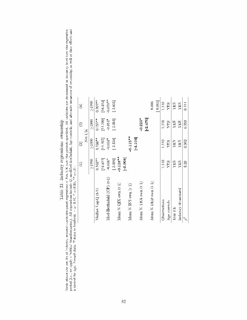
Table21:Industry

regressions:ow

nership

Tableshow

stheresultsofindustry

errors-in-variablespanelregressionsofNet

I/Kover

theperiodsspeci�ed.Allvariablesare

de-meaned

atindustry

levelover

theregression

period(i.e.,weapply

a`within'transform

ation).AllregressionsincludeQ,modi�ed

Her�ndahl,Agecontrols,andalternate

measuresofow

nership;aswellastimee�ects

and

acontrolforage.

Annualdata.T-statsin

brackets.+p<0.10,*p<0.05,**p<.01. (1)

(2)

(3)

(4)

Net

I/K

≥1990

≥1990

≥1990

≥1990

MedianLog-Q

(t-1)

0.163**

0.138**

0.151**

0.202**

[16.812]

[14.467]

[14.299]

[16.313]

Mod-Her�ndahl(C

P)(t-1)

-0.056*

-0.053*

-0.054*

-0.070**

[-2.394]

[-2.458]

[-2.464]

[-2.851]

Mean%

QIX

own(t-1)

-0.118**

[-3.068]

Mean%

INSow

n(t-1)

-0.115**

[-4.104]

Mean%

TRAow

n(t-1)

-0.225*

[-2.470]

Mean%

DEDow

n(t-1)

-0.006

[-0.065]

Observations

1,110

1,110

1,110

1,110

Agecontrols

YES

YES

YES

YES

YearFE

YES

YES

YES

YES

Industry

de-meaned

YES

YES

YES

YES

ρ2

0.39

0.363

0.359

0.414

82

Table22:Firm

regressions:allexplanationsexceptgovernance

andshort-term

ism

Tableshow

stheresultsof�rm

-levelerrors-in-variablespanelregressionsofNet

CAPX/PPEover

theperiodsspeci�ed.Allvariablesare

de-meaned

at�rm

-orindustry-level

over

theregressionperiod,asnoted.Allregressionsincludeour`core'�rm

-levelexplanations:Q,measuresofcompetitionandquasi-indexer

ownership,aswellastimee�ects

and�rm

log-age.

Weaddadditionalexplanatory

variablesindividuallyin

columns1-7.Annualdata.T-statsin

brackets.+p<0.10,*p<0.05,**p<.01.

(1)

(2)

(3)

(4)

(5)

(6)

(7)

Net

CAPX/PPE

≥1990

≥2000

≥2000

≥2000

≥1990

≥1990

≥1990

Q(t-1)

0.218**

0.188**

0.212**

0.193**

0.216**

0.219**

0.218**

[39.291]

[12.062]

[32.393]

[25.068]

[34.527]

[39.341]

[33.609]

%QIX

ownMA2

-0.120**

-0.181**

-0.114**

-0.108**

-0.126**

-0.121**

-0.138**

[-6.765]

[-6.975]

[-5.926]

[-6.038]

[-6.732]

[-6.776]

[-6.773]

Mod-Her�ndahl(t-1)

-0.071**

-0.101*

-0.138**

-0.142**

-0.069*

-0.072**

-0.089**

[-2.639]

[-2.162]

[-3.208]

[-3.591]

[-2.446]

[-2.690]

[-2.942]

Ext�ndep

('96-'00)

0.001

[0.249]

Bankdep

('00)

-0.001

[-0.109]

AAto

AAArating('00)

-0.130**

[-5.179]

(Intanex

GW)/at(t-1)

0.313**

[5.481]

%foreignprof(t-1)

0.004

[1.037]

LogofReg

index

(t-1)

0.005

[0.547]

Observations

77,772

15,615

36,377

32,801

64,425

77,731

60,804

Agecontrols

YES

YES

YES

YES

YES

YES

YES

YearFE

YES

YES

YES

YES

YES

YES

YES

Firm

de-meaned

YES

NO

NO

NO

YES

YES

YES

Industry

de-meaned

NO

YES

YES

YES

NO

NO

NO

ρ2

0.263

0.3

0.397

0.321

0.249

0.264

0.248

83

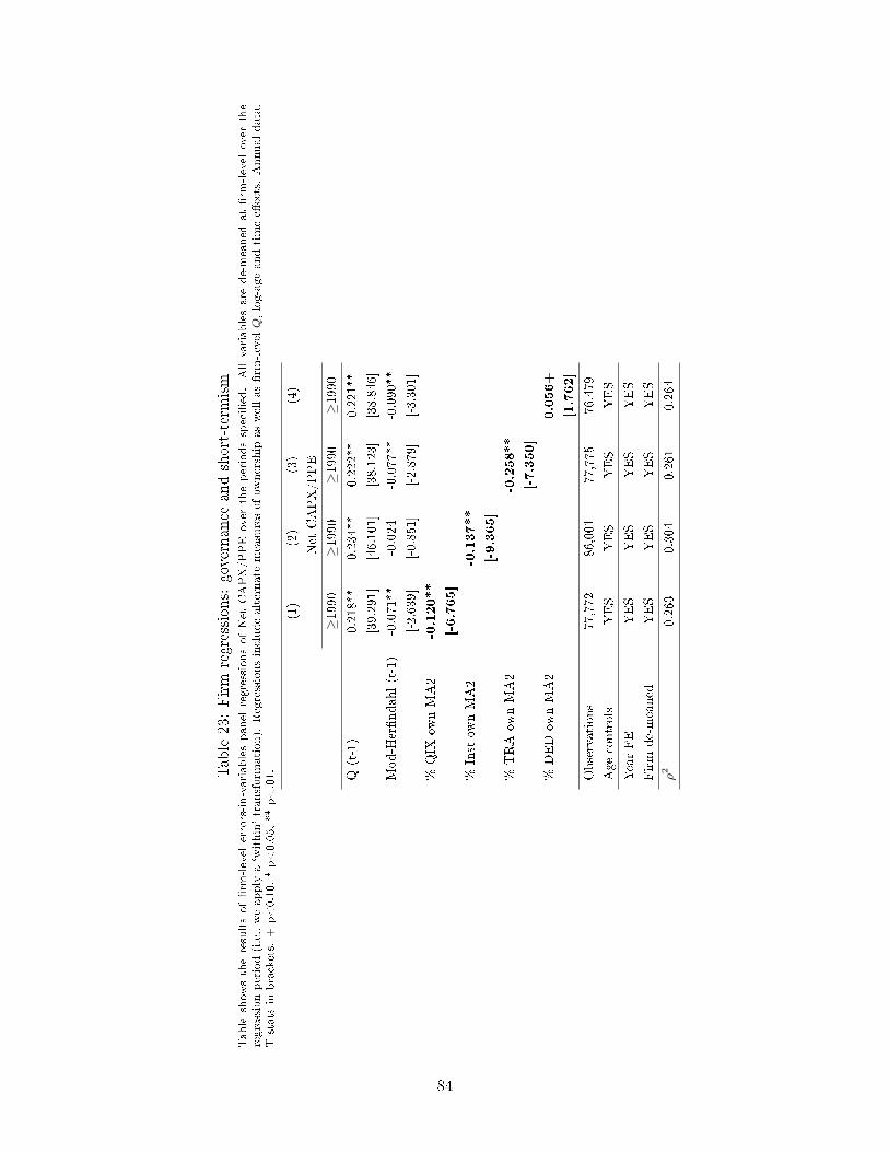
Table23:Firm

regressions:governance

andshort-term

ism

Table

show

stheresultsof�rm

-level

errors-in-variablespanel

regressionsofNet

CAPX/PPEover

theperiodsspeci�ed.Allvariablesare

de-meaned

at�rm

-level

over

the

regressionperiod(i.e.,weapply

a`within'transform

ation).Regressionsincludealternate

measuresofow

nership

aswellas�rm

-levelQ,log-ageandtimee�ects.Annualdata.

T-statsin

brackets.+p<0.10,*p<0.05,**p<.01.

(1)

(2)

(3)

(4)

Net

CAPX/PPE

≥1990

≥1990

≥1990

≥1990

Q(t-1)

0.218**

0.234**

0.222**

0.221**

[39.291]

[46.101]

[38.123]

[38.846]

Mod-Her�ndahl(t-1)

-0.071**

-0.024

-0.077**

-0.090**

[-2.639]

[-0.851]

[-2.879]

[-3.301]

%QIX

ownMA2

-0.120**

[-6.765]

%Inst

ownMA2

-0.137**

[-9.365]

%TRAow

nMA2

-0.258**

[-7.350]

%DEDow

nMA2

0.056+

[1.762]

Observations

77,772

86,001

77,775

76,479

Agecontrols

YES

YES

YES

YES

YearFE

YES

YES

YES

YES

Firm

de-meaned

YES

YES

YES

YES

ρ2

0.263

0.304

0.261

0.264

84

Table24:Post-2000

Industry

regressions:allexplanationsexceptcompetition

Table

show

stheresultsofindustry

errors-in-variablespanelregressionsofNet

I/K

over

theperiodsspeci�ed.Variablesare

de-meaned

atindustry

level

over

theregression

period(i.e.,weapply

a`within'transform

ation)wherenoted.Allregressionsincludeour`core'explanations:Q,modi�ed

Her�ndahlandquasi-indexer

ownership,aswellas

Agecontrols(m

eanlog-age),andtimee�ects.Weaddadditionalexplanatory

variablesonebyonein

columns2-6

andsimultaneously(when

signi�cantandproperly

signed)

incolumn7.Annualdata.T-stats

inbrackets.

+p<0.10,*p<0.05,**p<.01.

(1)

(2)

(3)

(4)

(5)

(6)

(7)

Net

I/K

≥2000

≥2000

≥2000

≥2000

≥2000

≥2000

≥2000

MedianLog-Q

(t-1)

0.163**

0.250**

0.246**

0.245**

0.165**

0.160**

0.162**

[13.130]

[11.643]

[12.814]

[14.513]

[14.762]

[12.691]

[14.355]

Mean%

QIX

own(t-1)†

-0.105**

-0.044

0.073

-0.078

-0.096*

-0.109**

-0.100**

[-2.657]

[-0.589]

[1.101]

[-1.017]

[-2.402]

[-2.865]

[-2.581]

Mod-Her�ndahl(t-1)†

-0.067+

-0.124**

-0.109**

-0.127**

-0.068+

-0.062+

-0.063+

[-1.844]

[-2.727]

[-2.950]

[-2.946]

[-1.907]

[-1.725]

[-1.796]

Meanext�ndep

('96-'00)

-0.007

[-0.672]

Mean%

bankdep

('96-'00)

0.104**

[3.828]

%ratedAAto

AAA('96-'00)

-0.328

[-1.225]

IPshare

ofinvestm

ent(t-1)

-0.040*

-0.039*

[-2.193]

[-2.131]

Mean%

foreignprof(t-1)‡

-0.028

-0.026

[-1.620]

[-1.465]

Observations

687

687

687

687

687

687

687

MeanAgecontrols

YES

YES

YES

YES

YES

YES

YES

YearFE

YES

YES

YES

YES

YES

YES

YES

Industry

de-meaned

YES

NO

NO

NO

YES

YES

YES

ρ2

0.431

0.699

0.683

0.673

0.446

0.428

0.443

†Quasi-indexer

ownership

andModi�ed

Her�ndahlmeasuredasthechangefrom

average1996-1999levelin

columns2,3and4

‡Foreignpro�tssetto

zero

ifmissing

85

Table25:Post-2000

Industry

regressions:competition

Tableshow

stheresultsofindustry

errors-in-variablespanelregressionsofNet

I/Kover

theperiodsspeci�ed.Allvariablesare

de-meaned

atindustry

levelover

theregression

period(i.e.,weapplya`within'transform

ation).AllregressionsincludeQ,quasi-indexerow

nership,agecontrols,timee�ects,andalternatemeasuresofcompetition.Her�ndahls,

Lerner

index

and(CompustatandCensus)concentrationappearsigni�cant.Annualdata.T-statsin

brackets.+p<0.10,*p<0.05,**p<.01.

(1)

(2)

(3)

(4)

(5)

(6)

(8)

(9)

(10)

Net

I/K

≥2000

≥2000

≥2000

≥2000

≥2000

≥2000

≥2000

≥2000

≥2000

MedianLog-Q

(t-1)

0.148**

0.163**

0.169**

0.158**

0.160**

0.132**

0.099+

0.095**

0.134**

[11.718]

[13.130]

[14.206]

[9.584]

[11.955]

[11.337]

[1.806]

[5.264]

[10.378]

Mean%

QIX

own(t-1)

-0.111**

-0.105**

-0.107**

-0.105*

-0.114**

-0.112**

-0.094**

-0.101*

-0.110**

[-2.807]

[-2.657]

[-2.708]

[-2.473]

[-2.871]

[-3.002]

[-2.582]

[-2.134]

[-2.912]

3Y

∆Log#ofFirms(t-1)

0.004

[0.287]

Mod-Her�ndahl(C

P)(t-1)

-0.067+

[-1.844]

SalesHer�ndahl(C

P)(t-1)

-0.089+

[-1.780]

CO

Herfadjustment(t-1)

-0.057+

[-1.677]

Lerner

Index

(t-1)

-0.054+

[-1.668]

%salesTop8(C

P)(t-1)

-0.092*

[-2.001]

%MVTop8(C

P)(t-1)

-0.018

[-0.859]

%salesin

Top50(C

ensus)

(t-1)‡

-0.054+

[-1.788]

LogofReg

index

(t-1)

-0.01

[-1.010]

%Licensed('08)

0

[-0.935]

Observations

687

687

687

687

687

687

571

478

687

Agecontrols

YES

YES

YES

YES

YES

YES

YES

YES

YES

YearFE

YES

YES

YES

YES

YES

YES

YES

YES

YES

Industry

de-meaned

YES

YES

YES

YES

YES

YES

YES

YES

YES

ρ2

0.429

0.431

0.44

0.455

0.449

0.404

0.447

0.343

0.408

‡When

agiven

BEAcategory

includes

more

thanoneNAICSLevel3code,weuse

thesales-weightedaverageofCensus-basedconcentrationsacross

allrelevantNAICSLevel

3categories.Only

consistentNAICSL3categories

included.Weinterpolate

concentrationbetweencensusyears

(e.g.,from

1997to

2002).

86

Table26:Post-2000

Firm

regressions:allexplanationsexceptgovernance

andshort-term

ism

Tableshow

stheresultsof�rm

-levelerrors-in-variablespanelregressionsofNet

CAPX/PPEover

theperiodsspeci�ed.Allvariablesare

de-meaned

at�rm

-orindustry-level

over

theregressionperiod,asnoted.Allregressionsincludeour`core'�rm

-levelexplanations:Q,measuresofcompetitionandQIX

ownership,aswellas�rm

log-ageandtime

e�ects.Weaddadditionalexplanatory

variablesindividuallyin

columns2-7.Annualdata.T-stats

inbrackets.

+p<0.10,*p<0.05,**p<.01.

(1)

(2)

(3)

(4)

(5)

(6)

(7)

Net

CAPX/PPE

≥2000

≥2000

≥2000

≥2000

≥2000

≥2000

≥2000

Q(t-1)

0.212**

0.188**

0.212**

0.193**

0.206**

0.212**

0.198**

[29.422]

[12.062]

[32.393]

[25.068]

[26.802]

[29.421]

[25.968]

%QIX

ownMA2

-0.071**

-0.181**

-0.114**

-0.108**

-0.082**

-0.071**

-0.102**

[-3.238]

[-6.975]

[-5.926]

[-6.038]

[-3.735]

[-3.234]

[-4.199]

Mod-Her�ndahl(t-1)

-0.074*

-0.101*

-0.138**

-0.142**

-0.078*

-0.074*

-0.081*

[-2.275]

[-2.162]

[-3.208]

[-3.591]

[-2.419]

[-2.273]

[-2.277]

Ext�ndep

('96-'00)

0.001

[0.249]

Bankdep

('00)

-0.001

[-0.109]

AAto

AAArating('00)

-0.130**

[-5.179]

(Intanex

GW)/at(t-1)

0.330**

[5.235]

%foreignprof(t-1)

0.001

[0.138]

LogofReg

index

(t-1)

-0.013

[-1.101]

Observations

45,264

15,615

36,377

32,801

41,163

45,253

34,538

Agecontrols

YES

YES

YES

YES

YES

YES

YES

YearFE

YES

YES

YES

YES

YES

YES

YES

Firm

de-meaned

YES

NO

NO

NO

YES

YES

YES

Industry

de-meaned

NO

YES

YES

YES

NO

NO

NO

ρ2

0.276

0.3

0.397

0.321

0.244

0.276

0.245

87

Table27:Post-2000

Firm

regressions:governance

andshort-term

ism

Table

show

stheresultsof�rm

-level

errors-in-variablespanel

regressionsofNet

CAPX/PPEover

theperiodsspeci�ed.Allvariablesare

de-meaned

at�rm

-level

over

the

regressionperiod(i.e.,weapply

a`within'transform

ation).

Regressionsincludealternate

measuresofgovernance

andshort-termism

aswellas�rm

-levelQ,log-ageandtime

e�ects.Annualdata.T-statsin

brackets.

+p<0.10,*p<0.05,**p<.01.

(1)

(2)

(3)

(4)

Net

CAPX/PPE

≥2000

≥2000

≥2000

≥2000

Q(t-1)

0.212**

0.234**

0.218**

0.215**

[29.422]

[35.168]

[28.756]

[28.949]

Mod-Her�ndahl(t-1)

-0.074*

-0.088*

-0.079*

-0.076*

[-2.275]

[-2.462]

[-2.372]

[-2.254]

%QIX

ownMA2

-0.071**

[-3.238]

%Inst

ownMA2

-0.134**

[-6.958]

%TRAow

nMA2

-0.226**

[-5.411]

%DEDow

nMA2

0.072+

[1.766]

Observations

45,264

48,849

45,267

43,971

Agecontrols

YES

YES

YES

YES

YearFE

YES

YES

YES

YES

Firm

de-meaned

YES

YES

YES

YES

ρ2

0.276

0.332

0.278

0.28

88

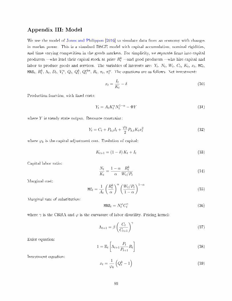
Appendix III: Model

We use the model of Jones and Philippon [2016] to simulate data from an economy with changes

in market power. This is a standard DSGE model with capital accumulation, nominal rigidities,

and time varying competition in the goods markets. For simplicity, we separate �rms into capital

producers � who lend their capital stock at price Rkt � and good producers � who hire capital and

labor to produce goods and services. The variables of interests are: Yt, Nt, Wt, Ct, Kt, xt, MCt,

MRSt, Rkt , Λt, Dt, V

nt , Qt, Q

kt , Q

obst , Rt, πt, π

wt . The equations are as follows. Net investment:

xt =ItKt− δ (30)

Production function, with �xed costs:

Yt = AtKαt N

1−αt − ΦY (31)

where Y is steady state output. Resource constraint:

Yt = Ct + Pk,tIt +ϕk2Pk,tKtx

2t (32)

where ϕk is the capital adjustment cost. Evolution of capital:

Kt+1 = (1− δ)Kt + It (33)

Capital-labor ratio:Nt

Kt=

1− αα

RktWt/Pt

(34)

Marginal cost:

MCt =1

At

(Rktα

)α(Wt/Pt1− α

)1−α(35)

Marginal rate of substitution:

MRSt = Nϕt C

γt (36)

where γ is the CRRA and ϕ is the curvature of labor disutility. Pricing kernel:

Λt+1 = β

(CtCt+1

)γ(37)

Euler equation:

1 = Et[Λt+1

PtPt+1

Rt

](38)

Investment equation:

xt =1

ϕk

(Qkt − 1

)(39)

89

Capital producing �rms:

Qkt = Et[βk

β

Λt+1

P kt

(Rkt+1 + P kt+1

(Qkt+1 − δ +

1

2ϕk

(Qkt+1 − 1

)2))](40)

where βk is the discount rate for (risky) corporate capital. Goods-producing (monopolists) �rms:

V nt = Dt + Et

[βk

βΛt+1V

nt+1

](41)

with real dividends

Dt = (1− MCt)AtKαt N

1−αt − ΦY (42)

Goods-producing Q:

Qt =Et[βk

β Λt+1Vnt+1

]P kt Kt+1

(43)

Total Q (mapped into observed Q in the data):

Qobst = Qkt +Qt (44)

Policy rule, taking into account the ZLB:

Rt = max

[1, Rφrt−1

(πptπ

)(1−φr)φπ (πwtπ

)(1−φr)φw (Nt

N

)(1−φr)φy]

(45)

Log-linear equations We take log-linear approximations of the above equations, together with

standard New Keynesian equations with Calvo stickiness in prices and wages.

πpt = βEt[πpt+1

]+ λpmct (46)

πwt = βEt[πwt+1

]+ λw (mrst − ωt) (47)

ωt = ωt−1 + πwt − πpt (48)

with λp ≡ (1−ϑp)(1−βϑp)ϑp

and λw ≡ (1−βϑw)(1−ϑw)ϑw

11+ϕεw

as in Gali [2008] and Woodford [2003].

Shocks Shocks in the log-linear equations.

1. Productivity:

at = ρaat−1 + εa,t

2. Demand/ZLB shock:

Et[λt+1 + rt − πpt+1

]= −ζdt

ζdt = ρdζdt−1 + εdt

90

3. Shock to the valuation of corporate assets:

qkt = Et[λt+1 + ζqt +

RkRk +Qk − δ

rk,t +Qk

Rk +Qk − δqkt

]vt = (1− β)dt + λt+1 + ζqt + βvt+1

qt = λt+1 + ζqt + vt+1 − kt1

ζqt = ρdζqt−1 + εqt

4. Shock to the policy rule:

rt = max [0, φrrt−1 + (1− φr) (φππt + φwwt + φyyt) + εr,t]

5. Transitory shock to markups:

πpt = βEt[πpt+1

]+ λpmct + ζet

ζet = ρeζet−1 + εet

In addition, there is a permanent shock to competition in the form of a unanticipated and permanent

change to the elasticity of substitution between intermediate goods.

Steady state Pk = 1, x = 0, Qk = 1, A = 1, mc =εp−1εp

Rk =1

βk− 1 + δ

(W/P )1−α = MC(1− α)1−α(Rk

α

)−αN/K =

1− αα

Rk

W/P

Y

K=

1

1 + Φ

(N

K

)1−α

C

K=Y

K− δ

Since wages are sticky, we have mrs = WP

(εw−1εw

), then:

Kϕ+γ = mrs

(C

K

)−γ (NK

)−ϕ

91

With K, we get the other steady-state aggregates.

V n =D

1− βk

Q =βkV n

K

Calibrated parameters Calibrate the following parameters. The discount factor used in the

valuation of corporate assets is βk < β. Risk aversion and Frisch elasticity taken from Smets and

Wouters [2007].

bet = 0.97^0.25 ;

betq = bet*0.96^0.25 ;

alph = 1/3 ; % technology capital share

varphi = 1.92 ; % disutility of labor

gamm = 1.4 ; % risk aversion

elasp = 6 ; % Subsitution across goods (initial value)

elasw = 6 ; % Subsitution labor types.

phifc = 0.1 ; % Fixed cost as fraction of output

delt = 0.025 ;

phik = 40 ; % Capital adjustment costs

Estimation Shocks and monetary policy parameters are estimated over 1984Q1 to 2015Q3. We

also estimate the ZLB duration, with the prior on each ZLB duration being derived from the NY

Federal Reserve survey of primary dealers.

92