NBER WORKING PAPER SERIES

INVESTMENT DISPERSION AND THE BUSINESS CYCLE

Rüdiger BachmannChristian Bayer

Working Paper 16861http://www.nber.org/papers/w16861

NATIONAL BUREAU OF ECONOMIC RESEARCH1050 Massachusetts Avenue

Cambridge, MA 02138March 2011

We thank Giuseppe Moscarini and Matthew Shapiro for his comments. We are grateful to seminar/meetingparticipants at Amsterdam, the ASSA (San Francisco), Bonn, Duke, ECARES (Brussels), ESSIM2009, Georgetown, Groningen, Johns Hopkins, Innsbruck, Michigan-Ann Arbor, Michigan State, MinneapolisFED, Notre Dame, Regensburg, SED (Istanbul), Wisconsin-Madison and Zürich for their comments.We thank the staff of the Research Department of Deutsche Bundesbank for their assistance. Specialthanks go to Timm Koerting for excellent research assistance. The views expressed herein are thoseof the authors and do not necessarily reflect the views of the National Bureau of Economic Research.

NBER working papers are circulated for discussion and comment purposes. They have not been peer-reviewed or been subject to the review by the NBER Board of Directors that accompanies officialNBER publications.

© 2011 by Rüdiger Bachmann and Christian Bayer. All rights reserved. Short sections of text, notto exceed two paragraphs, may be quoted without explicit permission provided that full credit, including© notice, is given to the source.

Investment Dispersion and the Business CycleRüdiger Bachmann and Christian BayerNBER Working Paper No. 16861March 2011JEL No. E2,E22,E3,E32

ABSTRACT

We document a new business cycle fact: the cross-sectional standard deviation of firm-level investment(investment dispersion) is robustly and significantly procyclical. This makes investment dispersiondifferent from the dispersion of productivity and output growth, which is countercyclical. Investmentdispersion is more procyclical in the goods-producing sectors, for smaller firms and for structures.We show that a heterogeneous-firm real business cycle model with countercyclical idiosyncratic firmrisk and non-convex adjustment costs calibrated to match moments of the long-run investment ratedistribution, produces a time series correlation coefficient between investment dispersion and aggregateoutput of 0.58, close to the 0.45 in the data. We argue, more generally, that cross-sectional businesscycle dynamics impose tight empirical restrictions on the physical environments and the structuralparameters of heterogeneous-firm models.

Rüdiger BachmannDepartment of EconomicsUniversity of MichiganLorch Hall 365BAnn Arbor, MI 48109-1220and NBERrudib@umich.edu

Christian BayerUniversität BonnDepartment of EconomicsAdenauerallee 24-4253113 BonnGermanychristian.bayer@uni-bonn.de

1 Introduction

Investment at the micro level is lumpy and infrequent (Doms and Dunne, 1998, Cooper and

Haltiwanger, 2006). The distribution of investment rates is positively skewed and has excess

kurtosis (Caballero et al., 1995). Motivated by these facts about the long-run cross-sectional

distribution of micro-level investment, researchers have studied models with non-convex cap-

ital adjustment costs and asked whether “getting the micro facts right” matters for aggregate

(investment) dynamics.1

In this paper we show that lumpy investment models have important and thus far unex-

plored implications for the dynamics of the cross-section of investment rates. Conversely, we

show that the joint dynamics of the cross-section of firm-level investment, output growth and

productivity growth provide important parameter restrictions for heterogeneous firm models.

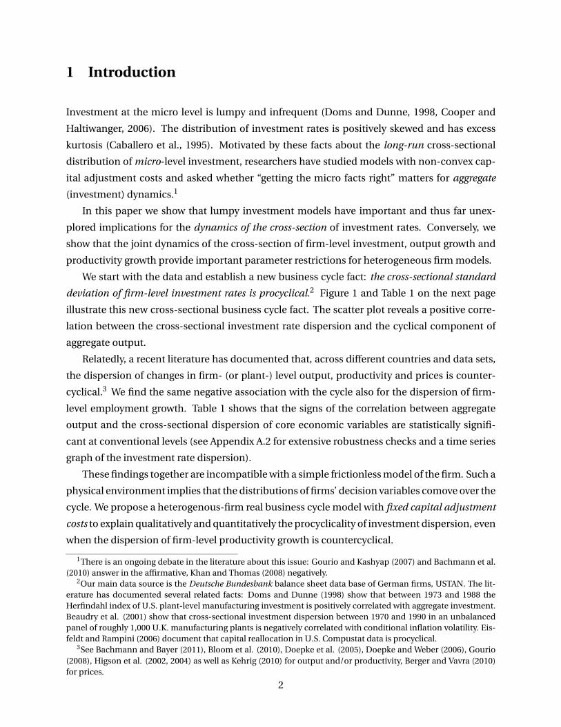
We start with the data and establish a new business cycle fact: the cross-sectional standard

deviation of firm-level investment rates is procyclical.2 Figure 1 and Table 1 on the next page

illustrate this new cross-sectional business cycle fact. The scatter plot reveals a positive corre-

lation between the cross-sectional investment rate dispersion and the cyclical component of

aggregate output.

Relatedly, a recent literature has documented that, across different countries and data sets,

the dispersion of changes in firm- (or plant-) level output, productivity and prices is counter-

cyclical.3 We find the same negative association with the cycle also for the dispersion of firm-

level employment growth. Table 1 shows that the signs of the correlation between aggregate

output and the cross-sectional dispersion of core economic variables are statistically signifi-

cant at conventional levels (see Appendix A.2 for extensive robustness checks and a time series

graph of the investment rate dispersion).

These findings together are incompatible with a simple frictionless model of the firm. Such a

physical environment implies that the distributions of firms’ decision variables comove over the

cycle. We propose a heterogenous-firm real business cycle model with fixed capital adjustment

costs to explain qualitatively and quantitatively the procyclicality of investment dispersion, even

when the dispersion of firm-level productivity growth is countercyclical.

1There is an ongoing debate in the literature about this issue: Gourio and Kashyap (2007) and Bachmann et al.(2010) answer in the affirmative, Khan and Thomas (2008) negatively.

2Our main data source is the Deutsche Bundesbank balance sheet data base of German firms, USTAN. The lit-erature has documented several related facts: Doms and Dunne (1998) show that between 1973 and 1988 theHerfindahl index of U.S. plant-level manufacturing investment is positively correlated with aggregate investment.Beaudry et al. (2001) show that cross-sectional investment dispersion between 1970 and 1990 in an unbalancedpanel of roughly 1,000 U.K. manufacturing plants is negatively correlated with conditional inflation volatility. Eis-feldt and Rampini (2006) document that capital reallocation in U.S. Compustat data is procyclical.

3See Bachmann and Bayer (2011), Bloom et al. (2010), Doepke et al. (2005), Doepke and Weber (2006), Gourio(2008), Higson et al. (2002, 2004) as well as Kehrig (2010) for output and/or productivity, Berger and Vavra (2010)for prices.

2

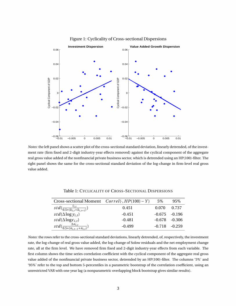
Figure 1: Cyclicality of Cross-sectional Dispersions

−0.01 −0.005 0 0.005 0.01−0.06

−0.04

−0.02

0

0.02

0.04

0.06C

yclic

al C

ompo

nent

of G

DP

Investment Dispersion

−0.01 −0.005 0 0.005 0.01−0.06

−0.04

−0.02

0

0.02

0.04

0.06

Cyc

lical

Com

pone

nt o

f GD

P

Value Added Growth Dispersion

Notes: the left panel shows a scatter plot of the cross-sectional standard deviation, linearly detrended, of the invest-

ment rate (firm fixed and 2-digit industry-year effects removed) against the cyclical component of the aggregate

real gross value added of the nonfinancial private business sector, which is detrended using an HP(100)-filter. The

right panel shows the same for the cross-sectional standard deviation of the log-change in firm-level real gross

value added.

Table 1: CYCLICALITY OF CROSS-SECTIONAL DISPERSIONS

Cross-sectional Moment Cor r el (·, HP (100)−Y ) 5% 95%

std(ii ,t

0.5∗(ki ,t+ki ,t+1) ) 0.451 0.070 0.737

std(∆ log yi ,t ) -0.451 -0.675 -0.196std(∆ logεi ,t ) -0.481 -0.678 -0.306

std(∆ni ,t

0.5∗(ni ,t−1+ni ,t ) ) -0.499 -0.718 -0.259

Notes: the rows refer to the cross-sectional standard deviations, linearly detrended, of, respectively, the investment

rate, the log-change of real gross value added, the log-change of Solow residuals and the net employment change

rate, all at the firm level. We have removed firm fixed and 2-digit industry-year effects from each variable. The

first column shows the time series correlation coefficient with the cyclical component of the aggregate real gross

value added of the nonfinancial private business sector, detrended by an HP(100)-filter. The columns ‘5%’ and

‘95%’ refer to the top and bottom 5-percentiles in a parametric bootstrap of the correlation coefficient, using an

unrestricted VAR with one year lag (a nonparametric overlapping block bootstrap gives similar results).

3

Fixed capital adjustment costs lead to nonlinear, two-step investment rules at the firm-level.

First, firms have a discrete decision whether to adjust or not to adjust (extensive margin). Sec-

ond, conditional on adjustment, firms decide by how much (intensive margin). The cross-

sectional investment dispersion is in general a complicated nonlinear function of both steps.

To fix ideas, eliminate the intensive margin decision and consider the case where firms can

only increase their capital stock by a given percentage or let it depreciate. In this case, both the

cross-sectional average and dispersion of investment are solely determined by how many firms

adjust. Average investment is increasing in the fraction of firms adjusting. And so is the disper-

sion of investment if less than half of the firms invest. Hence, as long as average investment is

procyclical, the cross-sectional investment dispersion is procyclical, too.

Of course, in reality and in realistic quantitative models both the extensive and the intensive

margins of capital adjustment are operative and multiple shocks hit the economy. We calibrate

our model (i) to match the deviations from normality in the steady-state investment rate dis-

tribution, and (ii) to the observed joint stochastic process for aggregate Solow residuals and

firm-level productivity growth dispersions, and show in Section 5 that such a model can quan-

titatively match the procyclicality of investment dispersion in the data.

This important result provides a new validation of the lumpy investment model. More gen-

erally, we argue that a fully fledged business cycle theory from the bottom up has to and can -

as we show - successfully speak to the dynamics of more than just the cross-sectional means of

the distributions underlying macroeconomic aggregates. We view this paper as a step towards

such a research program.

Why is this direction of research important? Heterogenous-firm models have seen increased

use in the macroeconomic and international finance literature. This paper argues (see Sec-

tion 5) that cross-sectional dynamics impose tight restrictions on physical environments and

structural parameters in these models. For instance, we show that procyclical investment dis-

persion – generated by a procyclical extensive margin effect – requires curvature in the firm’s

revenue function, for this procyclical extensive margin effect to be quantitatively relevant. Only

with substantial curvature rely firms mostly on the extensive margin for capital adjustment, as

large investments would put the firm too far off its optimal scale of operation (see Gourio and

Kashyap (2007) for a related observation). We also argue that matching jointly the cyclicality of

the dispersion of investment and output growth restricts cyclical fluctuations in firm-level pro-

ductivity risk, which have been recently studied in a variety of models by Arellano et al. (2010),

Bloom et al. (2010), Chugh (2009), Gilchrist, Sim and Zakrajsek (2009) as well as Schaal (2010).

We finally show that general equilibrium price movements are crucial to match quantitatively

cross-sectional firm dynamics, a conjecture by Khan and Thomas (2008).

4

2 The Facts

When cross-sectional dispersion is concerned, Davis et al. (2006) show that studying only pub-

licly traded firms (Compustat) can lead to wrong conclusions. Therefore, we use the Deutsche

Bundesbank balance sheet data base of German firms, USTAN. USTAN is a private sector, an-

nual, firm-level data set that allows us to make use of 26 years of data (1973-1998), with cross-

sections that have, on average, over 30,000 firms per year. USTAN has a broader ownership, firm

size and industry coverage than the available comparable U.S. data sets from Compustat and

the Annual Survey of Manufacturers. This allows us to study industry and size differences in the

behavior of the cross-section of firms over the business cycle.4

The evidence presented in the Introduction derived from the entire nonfinancial private

business sector, which includes firms that are in one of the following six 1-digit industries: agri-

culture, mining and energy, manufacturing, construction, trade, transportation and communi-

cation. This Section provides additional evidence that is highly suggestive of the mechanism

we exploit in this paper. 1) Across 2-digit industries there is a positive association between the

cyclicality of the extensive margin of investment and the cyclicality of the investment rate dis-

persion. 2) In the goods-producing sectors, like manufacturing and construction, where we

would expect non-convex capital adjustment to be most important, the investment rate dis-

persion is particularly procyclical. 3) The procyclicality of investment dispersion is declining

in firm size, consistent with the view that larger firms can partially outgrow adjustment costs.

4) Investment dispersion is less procyclical for equipment than it is for structures, which often

constitute by their very nature large and indivisible investment projects.

For firm-level employment adjustment rates we use the symmetric adjustment rate defini-

tion proposed in Davis et al. (1996),∆ni ,t

0.5∗(ni ,t−1+ni ,t ) ; and, analogously, for firm-level investment

rates:ii ,t

0.5∗(ki ,t+ki ,t+1) . To compute firm-level Solow residuals, we start, in accordance with our

model in Section 3, from the following Cobb-Douglas production function:

yi ,t = ztεi ,t kθi ,t nνi ,t ,

where εi ,t is firm-specific and zt aggregate productivity. We assume that labor input ni ,t is im-

mediately productive, whereas capital ki ,t is pre-determined and inherited from last period.

This difference is reflected in the different timing convention in the definitions of the invest-

ment and employment adjustment rates. We estimate the output elasticities of the production

factors, ν and θ, as median factor expenditures shares over gross value added within each in-

dustry.

4For details on the data set and the sample selection see Appendix A.1 as well as Bachmann and Bayer (2011).See Appendix A.2 for evidence on the cyclical behavior of investment dispersion from the UK DTI and the U.S.Compustat data bases.

5

We remove firm fixed and 2-digit industry-year effects from all four first-difference variables

in Table 1 to focus on idiosyncratic changes. We thus eliminate differences in industry-specific

responses to aggregate shocks as well as permanent ex-ante and predictable heterogeneity be-

tween firms.

We combine these firm-level data with annual national accounting data from Germany

(VGR) on gross value added, investment, capital and employment from two-digit industries.

We use these same VGR data to compute aggregate and industry-level Solow residuals.

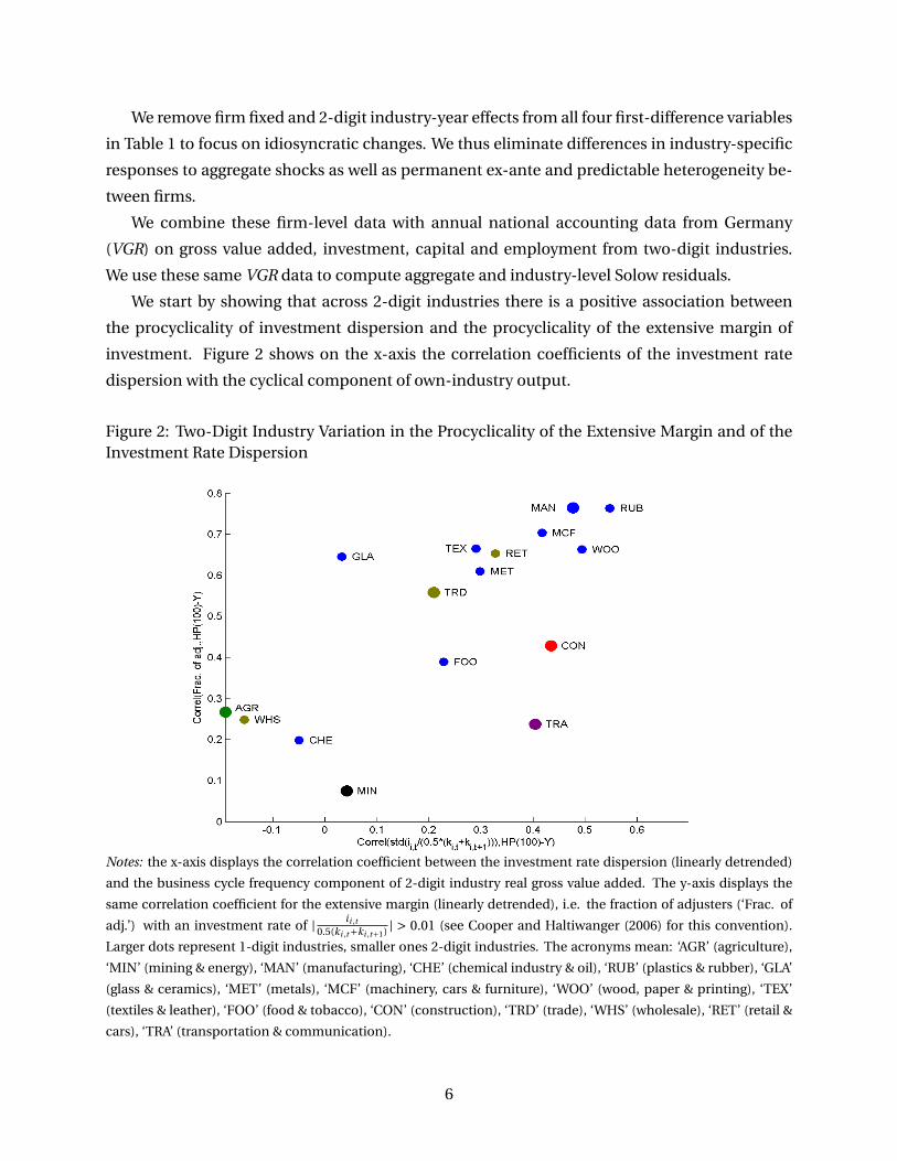
We start by showing that across 2-digit industries there is a positive association between

the procyclicality of investment dispersion and the procyclicality of the extensive margin of

investment. Figure 2 shows on the x-axis the correlation coefficients of the investment rate

dispersion with the cyclical component of own-industry output.

Figure 2: Two-Digit Industry Variation in the Procyclicality of the Extensive Margin and of theInvestment Rate Dispersion

Notes: the x-axis displays the correlation coefficient between the investment rate dispersion (linearly detrended)

and the business cycle frequency component of 2-digit industry real gross value added. The y-axis displays the

same correlation coefficient for the extensive margin (linearly detrended), i.e. the fraction of adjusters (‘Frac. of

adj.’) with an investment rate of | ii ,t0.5(ki ,t+ki ,t+1) | > 0.01 (see Cooper and Haltiwanger (2006) for this convention).

Larger dots represent 1-digit industries, smaller ones 2-digit industries. The acronyms mean: ‘AGR’ (agriculture),

‘MIN’ (mining & energy), ‘MAN’ (manufacturing), ‘CHE’ (chemical industry & oil), ‘RUB’ (plastics & rubber), ‘GLA’

(glass & ceramics), ‘MET’ (metals), ‘MCF’ (machinery, cars & furniture), ‘WOO’ (wood, paper & printing), ‘TEX’

(textiles & leather), ‘FOO’ (food & tobacco), ‘CON’ (construction), ‘TRD’ (trade), ‘WHS’ (wholesale), ‘RET’ (retail &

cars), ‘TRA’ (transportation & communication).

6

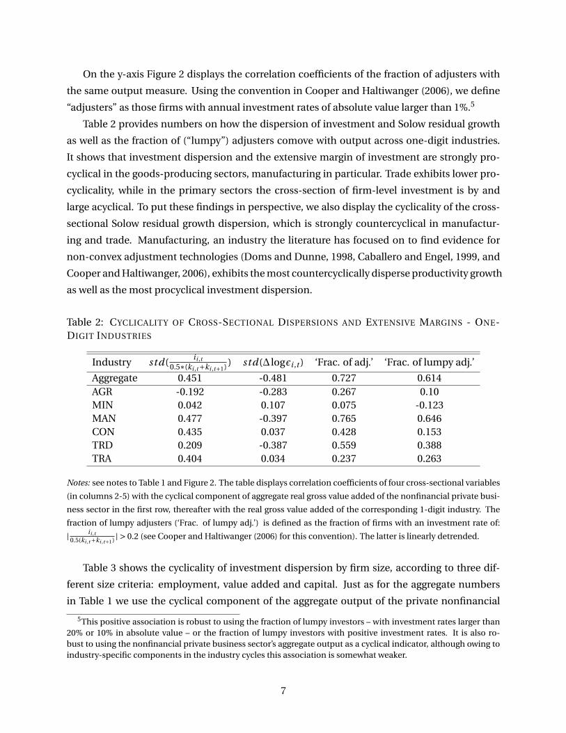
On the y-axis Figure 2 displays the correlation coefficients of the fraction of adjusters with

the same output measure. Using the convention in Cooper and Haltiwanger (2006), we define

“adjusters” as those firms with annual investment rates of absolute value larger than 1%.5

Table 2 provides numbers on how the dispersion of investment and Solow residual growth

as well as the fraction of (“lumpy”) adjusters comove with output across one-digit industries.

It shows that investment dispersion and the extensive margin of investment are strongly pro-

cyclical in the goods-producing sectors, manufacturing in particular. Trade exhibits lower pro-

cyclicality, while in the primary sectors the cross-section of firm-level investment is by and

large acyclical. To put these findings in perspective, we also display the cyclicality of the cross-

sectional Solow residual growth dispersion, which is strongly countercyclical in manufactur-

ing and trade. Manufacturing, an industry the literature has focused on to find evidence for

non-convex adjustment technologies (Doms and Dunne, 1998, Caballero and Engel, 1999, and

Cooper and Haltiwanger, 2006), exhibits the most countercyclically disperse productivity growth

as well as the most procyclical investment dispersion.

Table 2: CYCLICALITY OF CROSS-SECTIONAL DISPERSIONS AND EXTENSIVE MARGINS - ONE-DIGIT INDUSTRIES

Industry std(ii ,t

0.5∗(ki ,t+ki ,t+1) ) std(∆ logεi ,t ) ‘Frac. of adj.’ ‘Frac. of lumpy adj.’

Aggregate 0.451 -0.481 0.727 0.614AGR -0.192 -0.283 0.267 0.10MIN 0.042 0.107 0.075 -0.123MAN 0.477 -0.397 0.765 0.646CON 0.435 0.037 0.428 0.153TRD 0.209 -0.387 0.559 0.388TRA 0.404 0.034 0.237 0.263

Notes: see notes to Table 1 and Figure 2. The table displays correlation coefficients of four cross-sectional variables

(in columns 2-5) with the cyclical component of aggregate real gross value added of the nonfinancial private busi-

ness sector in the first row, thereafter with the real gross value added of the corresponding 1-digit industry. The

fraction of lumpy adjusters (‘Frac. of lumpy adj.’) is defined as the fraction of firms with an investment rate of:

| ii ,t0.5(ki ,t+ki ,t+1) | > 0.2 (see Cooper and Haltiwanger (2006) for this convention). The latter is linearly detrended.

Table 3 shows the cyclicality of investment dispersion by firm size, according to three dif-

ferent size criteria: employment, value added and capital. Just as for the aggregate numbers

in Table 1 we use the cyclical component of the aggregate output of the private nonfinancial

5This positive association is robust to using the fraction of lumpy investors – with investment rates larger than20% or 10% in absolute value – or the fraction of lumpy investors with positive investment rates. It is also ro-bust to using the nonfinancial private business sector’s aggregate output as a cyclical indicator, although owing toindustry-specific components in the industry cycles this association is somewhat weaker.

7

business sector as the cyclical indicator. We find procyclical investment dispersion mainly for

the smaller firms, especially when size is measured by employment or value added. The very

large firms, in contrast, have an almost acyclical investment dispersion. This distinction is sta-

tistically significant in the sense that if size is measured in terms of employment or value added,

neither the point estimate for the smallest size class lies in the [5%,95%]−bands of the largest

size class nor vice versa.

Table 3: CYCLICALITY OF CROSS-SECTIONAL INVESTMENT DISPERSION - FIRM SIZE

Size Class / Criterion Employment Value Added CapitalSmallest 25% 0.583 0.601 0.39125% to 50% 0.456 0.468 0.42250% to 75% 0.366 0.330 0.387Largest 25% 0.188 0.215 0.399Largest 5% 0.050 0.048 0.184

Notes: see notes to Table 1. The table displays correlation coefficients of the investment rate dispersion by firm size

with the cyclical component of the aggregate real gross value added of the private nonfinancial business sector.

This is at least consistent with the view that larger firms can smooth the effects of non-

convex capital adjustment costs and the extensive margin over several production units. Ta-

bles 2 and 3 also show that, while there is considerable variation in cross-sectional dynamics

across industries and firm sizes, our main empirical result that investment dispersion is pro-

cyclical is not driven by one large industry or the very large firms. We also find no evidence that

a large industry or the large firms have procyclical Solow residual growth dispersions, in which

case they could generate procyclical investment dispersion without any frictions (Bachmann

and Bayer (2011) documents this in more detail).

Table 4: CYCLICALITY OF CROSS-SECTIONAL INVESTMENT DISPERSION - TYPE OF CAPITAL GOOD

Aggregate Equipment Structures0.792 0.725 0.925

Notes: see notes to Table 1. The table displays correlation coefficients of the investment rate dispersion by

type of capital good with the linearly detrended cross-sectional average investment rate by type of capital good:

mean(ii ,t

0.5∗(ki ,t+ki ,t+1) ).

Finally, Table 4 shows the cyclicality of investment dispersion by type of capital good. Since

the average investment rate for structures is not very correlated with the overall business cy-

cle, we now use the linearly detrended cross-sectional average investment rate for equipment

and structures, respectively, as cyclical indicator. We find that the investment dispersion of

8

structures is almost perfectly correlated with the cycle in aggregate structural investment. We

interpret this as evidence that the extensive margin effect on cross-sectional investment disper-

sion is larger for structures, consistent with the available evidence that investment in structures

is subject to higher fixed adjustment costs (see Caballero and Engel, 1999).

Altogether, we view the evidence gathered in this section as at least suggestive that non-

convex capital adjustment costs have a role to play in explaining procyclical investment dis-

persion. We show next that quantitatively realistic fixed capital adjustment costs can indeed

generate procyclical investment dispersion, in the magnitude observed in the data.

3 The Model

Our model follows closely the real business cycle models in Khan and Thomas (2008) as well

as Bachmann et al. (2010). The main departure from either paper is that we introduce a sec-

ond aggregate shock, namely to the the standard deviation of idiosyncratic productivity shocks.

Such a shock is a convenient way to generate the observed countercyclicality of the dispersion

of firm value added growth. Moreover, it is required by the quantitative nature of our exercise,

as we will show that without it, even for very small fixed costs of capital adjustment, the ex-

tensive margin effect is so strong that the business cycle and investment dispersion are almost

perfectly correlated.

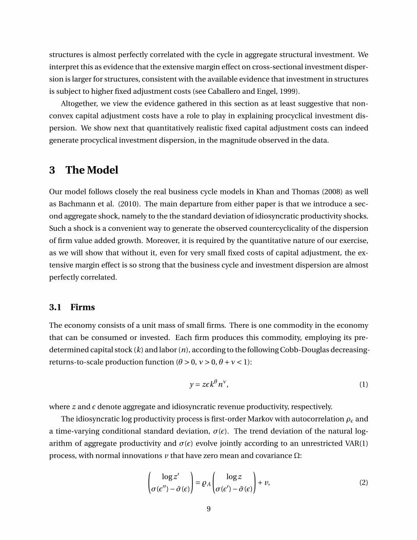
3.1 Firms

The economy consists of a unit mass of small firms. There is one commodity in the economy

that can be consumed or invested. Each firm produces this commodity, employing its pre-

determined capital stock (k) and labor (n), according to the following Cobb-Douglas decreasing-

returns-to-scale production function (θ > 0, ν> 0, θ+ν< 1):

y = zεkθnν, (1)

where z and ε denote aggregate and idiosyncratic revenue productivity, respectively.

The idiosyncratic log productivity process is first-order Markov with autocorrelation ρε and

a time-varying conditional standard deviation, σ(ε). The trend deviation of the natural log-

arithm of aggregate productivity and σ(ε) evolve jointly according to an unrestricted VAR(1)

process, with normal innovations v that have zero mean and covarianceΩ:(log z ′

σ(ε′′)− σ(ε)

)= %A

(log z

σ(ε′)− σ(ε)

)+ v, (2)

9

where σ(ε) denotes the steady state standard deviation of idiosyncratic productivity shocks.

We make a timing assumption that gives shocks toσ(ε) the interpretation of uncertainty shocks:

firms today observe the standard deviation of idiosyncratic productivity shocks tomorrow.6 The

shocks to the exogenous aggregate states, v , and idiosyncratic productivity shocks are indepen-

dent. Idiosyncratic productivity shocks are independent across productive units. In contrast,

we do not impose any restrictions onΩ or %A ∈R2×2.

We denote the trend growth rate of aggregate productivity by (1−θ)(γ−1), so that aggregate

output and capital grow at rate γ− 1 along the balanced growth path. From now on we work

with k and y (and later aggregate consumption, C ) in efficiency units.

Each period a firm draws its current cost of capital adjustment, 0 ≤ ξ ≤ ξ, which is denom-

inated in units of labor, from a time-invariant distribution, G . G is a uniform distribution on

[0, ξ], common to all firms. Draws are independent across firms and over time, and employ-

ment is freely adjustable.

Upon investment, i , the firm incurs a fixed cost of ωξ, where ω is the current real wage.

Capital depreciates at rate δ. We can then summarize the evolution of the firm’s capital stock

(in efficiency units) between two consecutive periods, from k to k ′, as follows:

Fixed cost paid γk ′

i 6= 0: ωξ (1−δ)k + i

i = 0: 0 (1−δ)k

Given the i.i.d. nature of the adjustment costs, it is sufficient to describe differences across

firms and their evolution by the distribution of firms over (ε,k). We denote this distribution by

µ. Thus,(z,σ(ε′),µ

)constitutes the current aggregate state and µ evolves according to the law

of motion µ′ = Γ(z,σ(ε′),µ), which firms take as given.

To summarize: at the beginning of a period, a firm is characterized by its pre-determined

capital stock, its idiosyncratic productivity, and its capital adjustment cost. Given the aggregate

state, it decides its employment level, n, production and depreciation occurs, workers are paid,

and investment decisions are made. Then the period ends.

Next we describe the dynamic programming problem of a firm. We will take two shortcuts

(details can be found in Khan and Thomas, 2008). We state the problem in terms of utils of the

representative household (rather than physical units), and denote the marginal utility of con-

sumption by p = p(z,σ(ε′),µ

). Also, given the i.i.d. nature of the adjustment costs, continuation

values can be expressed without future adjustment costs.

6We have experimented with the other timing assumption, whereσ(ε) and z are jointly observed. The quantita-tive differences are small. Investment dispersion tends to be slightly more procyclical under this alternative timingassumption.

10

Let V 1(ε,k,ξ; z,σ(ε′),µ) denote the expected discounted value - in utils - of a firm that is in

idiosyncratic state (ε,k,ξ), given the aggregate state (z,σ(ε′),µ). Then the firm’s expected value

prior to the realization of the adjustment cost draw is given by:

V 0(ε,k; z,σ(ε′),µ) =∫ ξ

0V 1(ε,k,ξ; z,σ(ε′),µ)G(dξ). (3)

With this notation the dynamic programming problem becomes:

V 1(ε,k,ξ; z,σ(ε′),µ) = maxn

CF+max(Vno adj,maxk ′ [−AC+Vadj]), (4)

where CF denotes the firm’s flow value, Vno adj the firm’s continuation value if it chooses inaction

and does not adjust, and Vadj the continuation value, net of adjustment costs AC , if the firm

adjusts its capital stock. That is:

CF = [zεkθnν−ω(z,σ(ε′),µ)n]p(z,σ(ε′),µ), (5a)

Vno adj =βE[V 0(ε′, (1−δ)k/γ; z ′,σ(ε′′),µ′)], (5b)

AC = ξω(z,σ(ε′),µ)p(z,σ(ε′),µ), (5c)

Vadj =−i p(z,σ(ε′),µ)+βE[V 0(ε′,k ′; z ′,σ(ε′′),µ′)], (5d)

where both expectation operators average over next period’s realizations of the aggregate and

idiosyncratic shocks, conditional on this period’s values, and we recall that i = γk ′− (1−δ)k.

The discount factor, β, reflects the time preferences of the representative household.

Taking as given ω(z,σ(ε′),µ) and p(z,σ(ε′),µ), and the law of motion µ′ = Γ(z,σ(ε′),µ), the

firm chooses optimally labor demand, whether to adjust its capital stock at the end of the pe-

riod, and the optimal capital stock, conditional on adjustment. This leads to policy functions:

N = N (ε,k; z,σ(ε′),µ) and K = K (ε,k,ξ; z,σ(ε′),µ). Since capital is pre-determined, the optimal

employment decision is independent of the current adjustment cost draw.

3.2 Households

We assume a continuum of identical households that have access to a complete set of state-

contingent claims. Hence, there is no heterogeneity across households. They own shares in

the firms and are paid dividends. We do not need to model the household side in detail (see

Khan and Thomas (2008) for that), we just use the first-order conditions that determine the

equilibrium wage and the marginal utility of consumption.

11

Households have a standard felicity function in consumption and labor:7

U (C , N h) = logC − AN h , (6)

where C denotes consumption and N h the household’s labor supply. Households maximize the

expected present discounted value of the above felicity function. By definition we have:

p(z,σ(ε′),µ) ≡UC (C , N h) = 1

C (z,σ(ε′),µ), (7)

and from the intratemporal first-order condition:

ω(z,σ(ε′),µ) =− UN (C , N h)

p(z,σ(ε′),µ)= A

p(z,σ(ε′),µ). (8)

3.3 Recursive Equilibrium

A recursive competitive equilibrium for this economy is a set of functions(ω, p,V 1, N ,K ,C , N h ,Γ

),

that satisfy

1. Firm optimality: Taking ω, p and Γ as given, V 1(ε,k; z,σ(ε′),µ) solves (4) and the corre-

sponding policy functions are N (ε,k; z,σ(ε′),µ) and K (ε,k,ξ; z,σ(ε′),µ).

2. Household optimality: Taking ω and p as given, the household’s consumption and labor

supply satisfy (7) and (8).

3. Commodity market clearing:

C (z,σ(ε′),µ) =∫

zεkθN (ε,k; z,σ(ε′),µ)νdµ −∫ ∫ ξ

0[γK (ε,k,ξ; z,σ(ε′),µ)− (1−δ)k]dGdµ.

4. Labor market clearing:

N h(z,σ(ε′),µ) =∫

N (ε,k; z,σ(ε′),µ)dµ +∫ ∫ ξ

0ξJ

(γK (ε,k,ξ; z,σ(ε′),µ)− (1−δ)k

)dGdµ,

where J (x) = 0, if x = 0 and 1, otherwise.

7We have experimented with a CRRA of 3 without much impact on our results.

12

5. Model consistent dynamics: The evolution of the cross-section that characterizes the econ-

omy, µ′ = Γ(z,σ(ε′),µ), is induced by K (ε,k,ξ; z,σ(ε′),µ) and the exogenous processes for

z, σ(ε′) as well as ε.

Conditions 1, 2, 3 and 4 define an equilibrium given Γ, while step 5 specifies the equilibrium

condition for Γ.

3.4 Solution

It is is well-known that (4) is not computable, because µ is infinite dimensional. We follow

Krusell and Smith (1997, 1998) and approximate the distribution, µ, by its first moment over

capital, k, and its evolution, Γ, by a simple log-linear rule. In the same vein, we approximate the

equilibrium pricing function by a log-linear rule, discrete aggregate state by discrete aggregate

state:

log k ′ =ak(z,σ(ε′)

)+bk(z,σ(ε′)

)log k, (9a)

log p =ap(z,σ(ε′)

)+bp(z,σ(ε′)

)log k, (9b)

Given (8), we do not have to specify an equilibrium rule for the real wage. As usual with the

Krusell and Smith procedure, we posit the log-linear forms (9a)–(9b) and check that in equilib-

rium they yield a good fit to the actual law of motion.

Substituting k for µ into (4) and using (9a)–(9b), (4) becomes a computable dynamic pro-

gramming problem with policy functions N = N (ε,k; z,σ(ε′), k) and K = K (ε,k,ξ; z,σ(ε′), k). We

solve this problem by value function iteration on V 0. We do so by applying multivariate spline

techniques that allow for a continuous choice of capital when the firm adjusts.

With these policy functions, we can then simulate a model economy without imposing the

equilibrium pricing rule (9b). Rather, we impose market-clearing conditions and solve for the

pricing kernel at every point in time of the simulation. We simulate the model economy for a

large number of time periods. This generates a time series of pt and kt endogenously, on

which the assumed rules (9a)–(9b) can be updated with a simple OLS regression. The proce-

dure stops when the updated coefficients ak(z,σ(ε′)

)to bp

(z,σ(ε′)

)are sufficiently close to the

previous ones.

13

4 Calibration

The model period is a year. This corresponds to the data frequency in USTAN. Most firm-level

data sets that are based on balance sheet data are of that frequency. The following parameters

then have standard values: β = 0.98 and δ = 0.094, which we compute from German national

accounting data for the nonfinancial private business sector. Given this depreciation rate, we

pick γ= 1.014, in order to match the time-average aggregate investment rate in the nonfinancial

private business sector: 0.108. γ= 1.014 is also consistent with German long-run growth rates.

The disutility of work parameter, A, is chosen to generate an average time spent at work of 0.33:

A = 2. We set the output elasticities of labor and capital to ν = 0.5565 and θ = 0.2075, respec-

tively, which correspond to the measured median labor and capital shares in manufacturing in

the USTAN data base.8

We measure the steady state standard deviation of idiosyncratic productivity shocks as σ(ε) =0.1201. Since idiosyncratic productivity shocks in the data also exhibit above-Gaussian kur-

tosis - 4.4480 on average -, and since the fixed adjustment costs parameters will be identi-

fied by the kurtosis of the firm-level investment rate (together with its skewness), we want to

avoid attributing excess kurtosis in the firm-level investment rate to lumpy investment, when

the idiosyncratic driving force itself has excess kurtosis. We incorporate the measured excess

kurtosis into the discretization process for the idiosyncratic productivity state by using a mix-

ture of two Gaussian distributions: N (0,0.0777) and N (0,0.1625) - the standard deviations are

0.1201 ± 0.0424, with a weight of 0.4118 on the first distribution. Finally, we set ρε = 0.95.

This process is discretized on a 19−state-grid, using Tauchen’s (1986) procedure with mixed

Gaussian normals. Heteroskedasticity in the idiosyncratic productivity process is modeled with

time-varying transition matrices between idiosyncratic productivity states, where the matrices

correspond to different values of σ(ε′).

To calibrate the parameters of the two-state aggregate shock process we estimate a bivariate,

unrestricted VAR with the linearly detrended natural logarithm of the aggregate Solow residual9

and the linearly detrended σ(ε′)-process from the USTAN data. The parameters of this VAR

are:10

%A =(

0.4474 −3.7808

0.0574 0.6952

)Ω=

(0.0146 0.1617

0.1617 0.0023

)(10)

This process is discretized on a [5×5]−state grid, using a bivariate analog of Tauchen’s proce-

dure.8If one views the DRTS assumption as a mere stand-in for a CRTS production function with monopolistic com-

petition, than these choices would correspond to an employment elasticity of the underlying production functionof 0.7284 and a markup of 1

θ+ν = 1.31. The implied capital elasticity of the revenue function, θ1−ν is 0.47.

9We use ν= 0.5565 and θ = 0.2075 in these calculations.10With a slight abuse of notation, but for the sake of readability,Ω has standard deviations on the main diagonal

and correlations on the off diagonal.

14

Given the aforementioned set of parameters(β,δ,γ, A,ν,θ,%A,Ω, σ(ε),ρε

), we calibrate the

adjustment costs parameter, ξ, to minimize a quadratic form in the normalized differences be-

tween the time-average firm-level investment rate skewness produced by the model and the

data, as well as the time-average firm-level investment rate kurtosis:11

minξΨ(ξ) ≡ 0.5 ·

[(( 1

T

∑t

skewness(ii ,t

0.5∗ (ki ,t +ki ,t+1))(ξ)−2.1920

)/0.6956

)2+(( 1

T

∑t

kur tosi s(ii ,t

0.5∗ (ki ,t +ki ,t+1))(ξ)−20.0355

/5.5064)

)2]

. (11)

As can be seen from (11), the distribution of firm-level investment rates exhibits both substan-

tial positive skewness – 2.1920 – as well as excess kurtosis – 20.0355. Caballero et al. (1995)

document a similar fact for U.S. manufacturing plants. They also argue that non-convex capital

adjustment costs are an important ingredient to explain such a strongly non-Gaussian distri-

bution, given a close-to-Gaussian shock process. With fixed adjustment costs, firms have an

incentive to lump their investment activity together over time in order to economize on these

adjustment costs. Therefore, typical capital adjustments are large, which creates excess kurto-

sis. Making use of depreciation, firms can adjust their capital stock downward without paying

adjustment costs. This makes negative investments less likely and hence leads to positive skew-

ness in firm-level investment rates. We therefore use the skewness and kurtosis of firm-level

investment rates to identify ξ.

Table 5: CALIBRATION OF ADJUSTMENT COSTS - ξ

ξ Skewness Kurtosis Ψ(ξ) Adj. costs/Unit of Output

0 -0.0117 3.2893 19.2865 0%0.01 0.7840 5.0383 11.5154 1.5%0.1 1.9329 9.3329 3.9167 6.8%0.25 (BL) 2.5590 12.1591 2.3244 13.3%0.5 3.0683 14.7695 2.5016 23.3%0.75 3.3738 16.4950 3.2996 33.2%1 3.5927 17.8153 4.2171 43.3%5 4.8536 27.1159 16.2937 263.01%

Notes: ‘BL’ denotes the baseline calibration. Skewness and kurtosis refer to the time-average of the corresponding

cross-sectional moments of firm-level investment rates. The fourth column displays the value ofΨ in (11). The last

column shows the average adjustment costs conditional on adjustment as a fraction of the firm’s annual output.

11The normalization constants in (11) are, respectively, the time series standard deviation of the cross-sectionalinvestment rate skewness and the time series standard deviation of the cross-sectional investment rate kurtosis inthe data.

15

Table 5 shows that ξ is indeed identified in this calibration strategy, as cross-sectional skew-

ness and kurtosis of the firm-level investment rates are monotonically increasing in ξ. The min-

imum of Ψ is achieved for ξ = 0.25, which constitutes our baseline case. This implies average

costs conditional on adjustment equivalent to roughly 13% of annual firm-level value added,

which is in line with estimates from the U.S. (see Bloom (2009), Table IV, for an overview).

5 Results

5.1 Baseline Results

Can a dynamic stochastic general equilibrium model with persistent idiosyncratic productivity

shocks, countercyclical aggregate shocks to their dispersion and fixed capital adjustment costs,

calibrated to the long-run non-Gaussianity of the investment rate distribution, reproduce the

cyclicality of important cross-sectional dispersion measures? Table 6 says “yes”. The model

matches the cyclicality of the dispersion of firm-level investment rates, of value added growth

and of employment growth as well as the cyclicality of the extensive margin reasonably well.12

Table 6: CYCLICALITY OF CROSS-SECTIONAL DISPERSIONS AND THE EXTENSIVE MARGIN OF IN-VESTMENT - BASELINE MODEL

Cor r el (·, HP (100)−Y )Cross-sectional Moment Model Data

std(ii ,t

0.5∗(ki ,t+ki ,t+1) ) 0.521 0.451

std(∆ log yi ,t ) -0.417 -0.451

std(∆ni ,t

0.5∗(ni ,t−1+ni ,t ) ) -0.455 -0.499

Fraction of adjusters 0.425 0.727Fraction of lumpy adjusters 0.381 0.614

Notes: see notes to Tables 1 and 2. The table displays correlation coefficients with HP(100)-filtered aggregate

output. The column ‘Model’ refers to the correlation coefficients from a simulation of the baseline model.

A basic, albeit only partial intuition why lumpy capital adjustment is a suitable candidate to

explain procyclical investment dispersion, can be gleaned from a simple Ss-model as in Caplin

and Spulber (1987):

12Figure 4 in Appendix A.2 shows a simulated time path of investment dispersion from the baseline model thatdisplays positive comovement with aggregate output.

16

Proposition:

In a one-sided Ss-model with a fixed optimal adjustment policy (conditional on adjustment),

S − s, and where the fraction of adjusters is given by ∆kS−s , the variance of adjustments increases

with average adjustment if and only if the fraction of adjusters is smaller than 0.5.

Proof: Average adjustment in this environment is obviously ∆k. From this it follows that the

variance of adjustment is given by: (0−∆k)2(1− ∆k

S−s

)+ (

(S − s)−∆k)2

(∆k

S−s

)= ∆k(S − s −∆k),

which is increasing in ∆k if and only if ∆kS−s < 0.5.

This example shows that with sufficient inertia procyclical investment dispersion is gener-

ated by a procyclical extensive margin, as in this simple model all aggregate dynamics are driven

by the extensive margin. The intensive margin of adjustment, S − s, is fixed by assumption. Of

course, this example is rather stylized and our quantitative model has both an extensive and an

intensive margin of investment operating and two aggregate shocks hitting the economy.

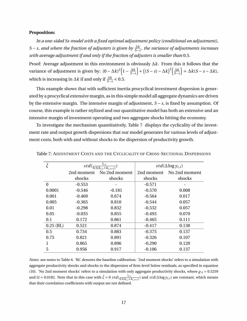
To investigate the mechanism quantitatively, Table 7 displays the cyclicality of the invest-

ment rate and output growth dispersions that our model generates for various levels of adjust-

ment costs, both with and without shocks to the dispersion of productivity growth.

Table 7: ADJUSTMENT COSTS AND THE CYCLICALITY OF CROSS-SECTIONAL DISPERSIONS

ξ std(ii ,t

0.5(ki ,t+ki ,t+1) ) std(∆ log yi ,t )

2nd moment No 2nd moment 2nd moment No 2nd momentshocks shocks shocks shocks

0 -0.553 - -0.571 -0.0001 -0.546 -0.181 -0.570 0.0080.001 -0.469 0.674 -0.564 0.0170.005 -0.365 0.810 -0.544 0.0570.01 -0.298 0.832 -0.532 0.0570.05 -0.035 0.855 -0.493 0.0700.1 0.172 0.861 -0.465 0.1110.25 (BL) 0.521 0.874 -0.417 0.1380.5 0.734 0.883 -0.375 0.1370.75 0.821 0.891 -0.326 0.1071 0.865 0.896 -0.290 0.1205 0.956 0.917 -0.106 0.137

Notes: see notes to Table 6. ‘BL’ denotes the baseline calibration. ‘2nd moment shocks’ refers to a simulation with

aggregate productivity shocks and shocks to the dispersion of firm-level Solow residuals, as specified in equation

(10). ‘No 2nd moment shocks’ refers to a simulation with only aggregate productivity shocks, where %A = 0.5259

and Ω = 0.0182. Note that in this case with ξ = 0 std(ii ,t

0.5(ki ,t+ki ,t+1) ) and std(∆ log yi ,t ) are constant, which means

that their correlation coefficients with output are not defined.

17

Two findings are important: the third and last column of Table 7 show that without second

moment shocks neither the procyclicality of the investment dispersion nor the countercycli-

cality of the output growth dispersion can be quantitatively replicated. Already a very small

non-convex capital adjustment cost generates procyclical investment dispersion – the gradient

of procyclicality in the adjustment cost factor, ξ, is steep. The model overshoots the number in

the data considerably. Also, without countercyclical second moment shocks the dispersion of

value added growth is essentially acyclial. Countercyclical second moment shocks are thus an

important part in understanding cross-sectional firm dynamics.

Secondly, in the presence of countercyclical second moment shocks, the procyclicality of

investment dispersion is a gradually and monotonically increasing function of the adjustment

cost parameter. What is perhaps surprising is that the same level of adjustment costs that best

matches the time average of the cross-sectional skewness and kurtosis of firm-level investment

rates - two statistics closely related to the extent of non-convexities at the micro-level as we have

explained in Section 4 - also makes the model match almost exactly the extent of procyclicality

of investment dispersion in the data, as measured by its correlation coefficient with the cyclical

component of output.

By contrast, in the frictionless case, ξ= 0, the dispersions of investment and output growth

merely mirror the countercyclicality of the dispersion of the idiosyncratic driving force, namely

idiosyncratic productivity. As the output growth dispersion is slightly too countercyclical for

ξ = 0, incidentally, non-convex capital adjustment costs help to align model and data also in

this dimension.

We view these results as a good validation of our mechanism and an example of the larger

premise of this paper that cross-sectional dynamics are an important aspect of the data that

heterogeneous firm models should address. In the presence of quantitatively realistic coun-

tercyclicality in the dispersion of firm-level Solow residual shocks, it is one level of adjustment

costs that jointly matches the time-average skewness and kurtosis of the investment rate distri-

bution and the time series correlation between the standard deviation of investment rates and

aggregate output. Moreover, such a model replicates the cyclicality of the cross-sectional dis-

persions of other important firm-level quantities. Table 7 shows that this identification is rather

tight.

Table 8 illustrates how the procyclicality of the investment dispersion and the procyclical-

ity of the extensive margin interact with the curvature of the firm’s revenue function, θ1−ν . The

results in columns three and four refer to setups with factor elasticities ν = 0.5333, θ = 0.2667

and ν= 0.5556, θ = 0.2778, respectively, compared to ν= 0.5565, θ = 0.2075 in the baseline sce-

nario.13 Larger revenue elasticities in capital imply lower procyclicality of the extensive margin

13In a monopolistic competition framework, column two implies a scenario with a CRTS-one-third-two-third

18

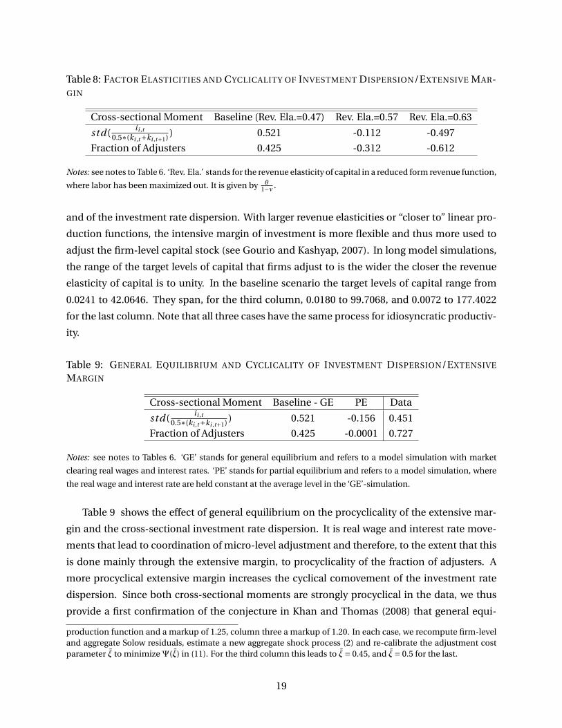
Table 8: FACTOR ELASTICITIES AND CYCLICALITY OF INVESTMENT DISPERSION/EXTENSIVE MAR-GIN

Cross-sectional Moment Baseline (Rev. Ela.=0.47) Rev. Ela.=0.57 Rev. Ela.=0.63

std(ii ,t

0.5∗(ki ,t+ki ,t+1) ) 0.521 -0.112 -0.497

Fraction of Adjusters 0.425 -0.312 -0.612

Notes: see notes to Table 6. ‘Rev. Ela.’ stands for the revenue elasticity of capital in a reduced form revenue function,

where labor has been maximized out. It is given by θ1−ν .

and of the investment rate dispersion. With larger revenue elasticities or “closer to” linear pro-

duction functions, the intensive margin of investment is more flexible and thus more used to

adjust the firm-level capital stock (see Gourio and Kashyap, 2007). In long model simulations,

the range of the target levels of capital that firms adjust to is the wider the closer the revenue

elasticity of capital is to unity. In the baseline scenario the target levels of capital range from

0.0241 to 42.0646. They span, for the third column, 0.0180 to 99.7068, and 0.0072 to 177.4022

for the last column. Note that all three cases have the same process for idiosyncratic productiv-

ity.

Table 9: GENERAL EQUILIBRIUM AND CYCLICALITY OF INVESTMENT DISPERSION/EXTENSIVE

MARGIN

Cross-sectional Moment Baseline - GE PE Data

std(ii ,t

0.5∗(ki ,t+ki ,t+1) ) 0.521 -0.156 0.451

Fraction of Adjusters 0.425 -0.0001 0.727

Notes: see notes to Tables 6. ‘GE’ stands for general equilibrium and refers to a model simulation with market

clearing real wages and interest rates. ‘PE’ stands for partial equilibrium and refers to a model simulation, where

the real wage and interest rate are held constant at the average level in the ‘GE’-simulation.

Table 9 shows the effect of general equilibrium on the procyclicality of the extensive mar-

gin and the cross-sectional investment rate dispersion. It is real wage and interest rate move-

ments that lead to coordination of micro-level adjustment and therefore, to the extent that this

is done mainly through the extensive margin, to procyclicality of the fraction of adjusters. A

more procyclical extensive margin increases the cyclical comovement of the investment rate

dispersion. Since both cross-sectional moments are strongly procyclical in the data, we thus

provide a first confirmation of the conjecture in Khan and Thomas (2008) that general equi-

production function and a markup of 1.25, column three a markup of 1.20. In each case, we recompute firm-leveland aggregate Solow residuals, estimate a new aggregate shock process (2) and re-calibrate the adjustment costparameter ξ to minimizeΨ(ξ) in (11). For the third column this leads to ξ= 0.45, and ξ= 0.5 for the last.

19

librium price movements are important to quantitatively account for cross-sectional business

cycle dynamics.

Table 10: VOLATILITY OF SECOND MOMENT SHOCKS AND CYCLICALITY OF INVESTMENT DISPER-SION/EXTENSIVE MARGIN

Cross-sectional Moment Baseline Double Volatility of Quadruple Volatility ofstd(∆ logεi ,t ) std(∆ logεi ,t )

std(ii ,t

0.5∗(ki ,t+ki ,t+1) ) 0.521 -0.070 -0.314

Fraction of Adjusters 0.425 -0.157 -0.335

Notes: see notes to Table 6. For the ‘Double Volatility of std(∆ logεi ,t )’-case, we use the data time series of

std(∆ logεi ,t ) multiplied by a factor 2 to reestimate the aggregate shock process (2) and recompute the equilib-

rium with an otherwise unaltered model specification. For the ‘Quadruple Volatility of std(∆ logεi ,t )’-case, we

multiply by a factor of 4.

With the final Table 10 we argue that it is important to match the cyclicality of the invest-

ment and the output growth dispersions jointly, and that the procyclicality of investment dis-

persion places tight bounds on the volatility of the second-moment shocks. If we increase this

volatility and make second moment shocks “more important”, the procyclicality of investment

dispersion is eliminated rather quickly.

In summary, both the procyclicality of investment dispersion as well as the countercycli-

cality of the dispersion of firm-level value added growth imposes rather tight restrictions on

important structural parameters, such as adjustment costs, factor elasticities in the production

function and the volatility of second moment shocks. This makes the study of cross-sectional

business cycle dynamics important for the calibration of heterogenous-firm models. We also

show that the nature of the aggregate environment - market clearing with flexible prices or not

- and cross-sectional business cycle dynamics are linked and should be jointly used to disci-

pline models.

5.2 Results from Industry Calibrations

We next use the one-digit industry variation in the procyclicality of investment dispersion and

the extensive margin depicted in Figure 2 in Section 2 and check whether the model can gener-

ate a similar variation. Instead of calibrating and computing a six-industry general equilibrium

model of the entire German economy, which would be computationally too burdensome, we

run six variants of our baseline model, where we adjust the important parameters to industry-

specific moments, but otherwise treat the corresponding industry as if it was the aggregate

economy. With this caveat in mind, we view this exercise as a useful additional test for the

extensive margin mechanism and its effect on cross-sectional dynamics.

20

Specifically, we calibrate the factor elasticities in the production function to the median in-

dustry income shares in USTAN and use the industry cuts from USTAN to compute the long-run

average and the time series process of the standard deviations of the firm-level Solow residual

shocks. We calibrate the depreciation rates to match the industry-specific long-run aggregate

investment rate from German national accounting data. The industry national accounting data

also allow us to compute industry-specific Solow residuals and then reestimate the VAR in equa-

tion (2). Finally, just as in the baseline calibration, we calibrate the adjustment costs parameter,

ξ, to minimize a quadratic form in industry-specific skewness and kurtosis of the firm-level

investment rates, analogous to (11).14

Table 11: RESULTS FROM INDUSTRY CALIBRATIONS

Industry std(ii ,t

0.5∗(ki ,t+ki ,t+1) ) Fraction of Adjusters

Model Data Model DataAggregate 0.521 0.451 0.425 0.727MIN 0.071 0.042 0.075 0.075MAN 0.776 0.477 0.760 0.765CON 0.698 0.435 0.580 0.428TRD 0.912 0.209 0.925 0.559TRA 0.281 0.404 0.299 0.237

Notes: see notes to Tables 2 and 6. See Figure 2 for the industry acronyms. The table displays correlation coeffi-

cients with HP(100)-filtered output. The column ‘Model’ refers to the correlation coefficients from model simula-

tions. The column ‘Data’ uses aggregate real gross value added of the nonfinancial private business sector in the

first row, thereafter the real gross value added of the corresponding 1-digit industry.

Table 11 displays the results for the correlations of investment dispersion and the extensive

margin with own-industry output.15 The correlation coefficients between model simulations

and data are 0.471 for the investment rate dispersion and 0.901 for the extensive margin. The

corresponding rank correlations are 0.4 and 0.9, respectively. The model captures the overall

variation rather well, with mining and energy not displaying any cyclicality of either investment

rate dispersion or the extensive margin, transportation and communication taking up a middle

position and manufacturing and construction having the strongest procyclicality. The biggest

exception is trade, where the model produces an almost perfect procyclicality of investment

14Table 18 in Appendix B collects the main parameters for each industry.15For computational reasons we leave out agriculture, for which we estimate a revenue elasticity of capital of

0.935. This would require extremely fine and large grids for firm-level capital. Given this low curvature of thefirm’s revenue function and our results in Table 8 from Section 5.1, the slightly negative correlation of investmentdispersion in agriculture supports the extensive margin mechanism ex negativo, making the cumbersome compu-tation unnecessary. For similar reasons, in the computation for the mining and energy sector we scale down themeasured factor elasticities by a factor of 0.9.

21

rate dispersion and the extensive margin, which is inconsistent with the data. We estimate the

revenue elasticity of capital for trade to be 0.403, the lowest value for any of the six one-digit

industries. This low curvature facilitates the extensive margin mechanism to an extent that

is obviously at odds with the data. We nevertheless view the industry-specific results overall

as additional support for the extensive margin mechanism and its relation to cross-sectional

dynamics, although, clearly, other things are going on, too.

6 Final Remarks

This paper establishes a new business cycle fact: the cross-sectional standard deviation of

firm-level investment is robustly and significantly procyclical. Investment dispersion is more

procyclical in the goods-producing sectors, for smaller firms and for structures. This paper

also shows that important structural parameters such as capital adjustment costs, the curva-

ture of the firms’ revenue function or the heteroskedasticity of the firm-level productivity pro-

cess have important implications for the dynamics of the cross-section of firms. This means,

conversely, that cross-sectional dynamics should be used in the calibration and evaluation of

heterogeneous-firm models. In such models the nature of the aggregate environment - mar-

ket clearing with flexible prices or not - and cross-sectional business cycle dynamics are tightly

linked and should be jointly used as a disciplining device.

We view this paper as just the beginning of a new research program that attempts to un-

derstand more comprehensively the time-series behavior of the entire cross-section of firms,

not merely the cyclicality of second moments. This will, hopefully, lead to a better microfoun-

dation and identification of structural heterogeneous-firm models and contribute to making

them better suitable for policy analysis.

22

References

[1] Arellano, C., Y. Bai, and P. Kehoe (2010). “Financial Markets and Fluctuations in Uncer-

tainty”, Federal Reserve Bank of Minneapolis Research Department Staff Report.

[2] Bachmann, R. and C. Bayer (2011). “The Cross-section of Firms”, mimeo University of

Michigan.

[3] Bachmann, R., Caballero, R. and E. Engel (2010). “Aggregate Implications of Lumpy Invest-

ment: New Evidence and a DSGE Model”, mimeo Yale University.

[4] Berger, D., and J. Vavra (2010). “The Dynamics of the U.S. Price Distribution”, mimeo Yale

University.

[5] Bloom, N. (2009). “The Impact of Uncertainty Shocks”, Econometrica, 77/3, 623–685.

[6] Bloom, N., M. Floetotto and N. Jaimovich (2010). “Really Uncertain Business Cycles”,

mimeo Stanford University.

[7] Caballero, R., E. Engel and J. Haltiwanger (1995). “Plant-Level Adjustment and Aggregate

Investment Dynamics”, Brookings Paper on Economic Activity, 1995, (2), 1–54.

[8] Caballero, R. and E. Engel (1999). “Explaining Investment Dynamics in U.S. Manufactur-

ing: A Generalized (S, s) Approach,” Econometrica, July 1999, 67(4), 741–782.

[9] Caplin, A. and D. Spulber (1987). “Menu Costs and the Neutrality of Money”, Quarterly

Journal of Economics, 102, 703–726.

[10] Chugh, S. (2009). “Firm Risk and Leverage-Based Business Cycles”, mimeo University of

Maryland.

[11] Cooper, R. and J. Haltiwanger (2006). “On the Nature of Capital Adjustment Costs”, Review

of Economic Studies, 73, 611–633.

[12] Davis, S., J. Haltiwanger and S. Schuh (1996). “Job Creation and Destruction”, Cambridge,

MA: MIT Press.

[13] Davis, S., J. Haltiwanger, R. Jarmin and J. Miranda (2006). “Volatility and Dispersion in

Business Growth Rates: Publicly Traded and Privately Held Firms”, NBER Macroeconomics

Annual.

23

[14] Doepke, J. and S. Weber (2006). “The Within-Distribution Business Cycle Dynamics of Ger-

man Firms”, Discussion Paper Series 1: Economic Studies, No 29/2006. Deutsche Bundes-

bank.

[15] Doepke, J., M. Funke, S. Holly and S. Weber (2005). “The Cross-Sectional Dynamics of

German Business Cycles: a Bird’s Eye View”, Discussion Paper Series 1: Economic Studies,

No 23/2005. Deutsche Bundesbank.

[16] Doms, M. and T. Dunne (1998). “Capital Adjustment Patterns in Manufacturing Plants”,

Review of Economic Dynamics, 1, 1998, 409–429.

[17] Eisfeldt, A. and A. Rampini (2006). “Capital Reallocation and Liquidity”, Journal of Mone-

tary Economics, 53, 369–399.

[18] Gilchrist, S., J. Sim and E. Zakrajsek (2010). “Uncertainty, Financial Frictions, and Invest-

ment Dynamics”, mimeo Boston University.

[19] Gourio, F. (2008). “Estimating Firm-Level Risk”, mimeo Boston University.

[20] Gourio, F. and A.K. Kashyap, (2007). “Investment Spikes: New Facts and a General Equi-

librium Exploration”, Journal of Monetary Economics, 54, 1–22.

[21] Heckman, J. (1976). “The common structure of statistical models of truncation, sample se-

lection, and limited dependent variables and a simple estimator for such models”, Annals

of Economic and Social Measurement, 5, 475–492.

[22] Higson, C., S. Holly and P. Kattuman (2002). “The Cross-Sectional Dynamics of the US

Business Cycle: 1950–1999”, Journal of Economic Dynamics and Control, 26, 1539–1555.

[23] Higson, C., S. Holly, P. Kattuman and S. Platis (2004): “The Business Cycle, Macroeconomic

Shocks and the Cross Section: The Growth of UK Quoted Companies”, Economica, 71/281,

May 2004, 299–318.

[24] von Kalckreuth, U. (2003). “Exploring the role of uncertainty for corporate investment de-

cisions in Germany”, Swiss Journal of Economics, Vol. 139(2), 173–206.

[25] Kehrig, M. (2010). “The Cyclicality of Productivity Dispersion”, mimeo Northwestern Uni-

versity.

[26] Khan, A. and J. Thomas, (2008). “Idiosyncratic Shocks and the Role of Nonconvexities in

Plant and Aggregate Investment Dynamics”, Econometrica, 76(2), March 2008, 395–436.

24

[27] Krusell, P. and A. Smith (1997). “Income and Wealth Heterogeneity, Portfolio Choice and

Equilibrium Asset Returns”, Macroeconomic Dynamics 1, 387–422.

[28] Krusell, P. and A. Smith (1998). “Income and Wealth Heterogeneity in the Macroeconomy”,

Journal of Political Economy, 106 (5), 867–896.

[29] Ravn, M. and H. Uhlig (2002). “On Adjusting the Hodrick-Prescott Filter for the Frequency

of Observations”, The Review of Economics and Statistics, 84 (2), 371–380.

[30] Schaal, E. (2010). “Uncertainty, Productivity and Unemployment in the Great Recession”,

mimeo Princeton University.

[31] Stoess, E. (2001). “Deutsche Bundesbank’s Corporate Balance Sheet Statistics and Areas of

Application”, Schmollers Jahrbuch: Zeitschrift fuer Wirtschafts- und Sozialwissenschaften

(Journal of Applied Social Science Studies), 121, 131–137

[32] Tauchen, G. (1986). “Finite State Markov-Chain Approximations To Univariate and Vector

Autoregressions”, Economics Letters 20, 177–181.

25

A Appendix - Data

A.1 Description of the Sample

Our firm-level data source is USTAN (Unternehmensbilanzstatistik) of Deutsche Bundesbank,

which is a large annual firm-level balance sheet data base. It provides annual firm level data

from 1971 to 1998 from the balance sheets and the profit and loss accounts of over 60,000 firms

per year. It originated as a by-product of the Bundesbank’s rediscounting and lending activities.

Bundesbank law required the Bundesbank to assess the creditworthiness of all parties backing

a commercial bill put up for discounting. It implemented this regulation by requiring balance

sheet data of all parties involved. These balance sheet data were then archived and collected

into a database (see Stoess (2001) and von Kalckreuth (2003) for details).

Although the sampling design – one’s commercial bill being put up for discounting – does

not lead to a perfectly representative selection of firms in a statistical sense, the coverage of the

sample is very broad. USTAN covers incorporated firms as well as privately-owned companies.

Its industry coverage – while still somewhat biased towards manufacturing firms – includes the

construction, the service as well as the primary sectors. The following Table 12 displays the

industry coverage of our final baseline sample.

Table 12: INDUSTRY COVERAGE

One-digit Industry Firm-year observations PercentageAgriculture 12,291 1.44Mining & Energy 4,165 0.49Manufacturing 405,787 47.50Construction 54,569 6.39Trade (Retail & Wholesale) 355,208 41.59Transportation & Communication 22,085 2.59

While there remains a bias towards larger and financially healthier firms, the size coverage

is still fairly broad: 31% of all firm-year observations in our final baseline sample have less than

20 employees and 57% have less than 50 employees. In terms of ownership structure, only 2%

of firm-year observations are from publicly traded firms, just under 60% from limited liability

companies and just under 40% from private firms with fully liable partners. Finally, the Bun-

desbank itself frequently uses the USTAN data for its macroeconomic analyses and for cross-

checking national accounting data. We take this as an indication that the bank considers the

data as sufficiently representative and of high quality. This makes the USTAN data a suitable

data source for the study of cross-sectional business cycle dynamics.

26

From the original USTAN data, we select only firms that report information on payroll, gross

value added (before depreciation) and capital stocks. Moreover, we drop observations from East

German firms to avoid a break of the series in 1990. We deflate all but the capital and investment

data by the implicit deflator for gross value added from the German national accounts.

Capital is deflated with one-digit industry- and capital-good specific investment good price

deflators within a perpetual inventory method. Similarly, we recover the amount of labor inputs

from wage bills (we calculate an average wage for cells of firms described by industry, year, firm-

size, and region and then divide the payroll by this average), as information on the number

of employees is only updated infrequently for some companies. Finally, the firm-level Solow

residual is calculated from data on real gross value added and factor inputs.

We remove outliers according to the following procedure: we calculate log changes in real

gross value added, the Solow residual, real capital and employment, as well as the firm-level

investment rate and drop all observations where a change falls outside a three standard devia-

tions interval around the year-specific mean. We also drop those firms for which we do not have

at least five observations in first differences. This leaves us with a sample of 854,105 firm-year

observations, which corresponds to observations on 72,853 firms, i.e. the average observation

length of a firm in the sample is 11.7 years. The average number of firms in the cross-section of

any given year is 32,850. Details on the implementation as well as the representativeness of the

resulting sample can be found in Bachmann and Bayer (2011).

27

A.2 Robustness

We start by showing in Table 13 that the cross-sectional averages of investment as well as out-

put, productivity and employment growth, computed from USTAN, are strongly positively cor-

related with the cyclical component of the real gross value added of the nonfinancial private

business sector. This means that USTAN represents well the cyclical behavior of the sectoral

aggregate it is meant to represent.

Table 13: CYCLICALITY OF CROSS-SECTIONAL AVERAGES

Cross-sectional Moment Cor r el (·, HP (100)−Y )

mean(ii ,t

0.5∗(ki ,t+ki ,t+1) ) 0.756

mean(∆ log yi ,t ) 0.663mean(∆ logεi ,t ) 0.592

mean(∆ni ,t

0.5∗(ni ,t−1+ni ,t ) ) 0.602

Notes: the table shows the time series correlation coefficient of cross-sectional averages, linearly detrended, with

the cyclical component of the aggregate real gross value added of the nonfinancial private business sector, which

we detrend using an HP(100)-filter. The rows refer, respectively, to the investment rate, the log-change of real gross

value added, the log-change of Solow residuals and the net employment change rate. We have removed firm fixed

and 2-digit industry-year effects from each variable.

The next two tables provide robustness checks for our main empirical result that the cross-

sectional investment rate dispersion is procyclical. We start by varying the cyclical indicator in

Table 14, while Table 15 deals with robustness related to the choice and treatment of the cross-

sectional dispersion measure as well as robustness with respect to general data treatment.

Table 14: CYCLICALITY OF CROSS-SECTIONAL INVESTMENT DISPERSION - ROBUSTNESS TO

CYCLICAL INDICATOR

Cyclical Indicator Cor r el (std(ii ,t

0.5∗(ki ,t+ki ,t+1) ), ·)Baseline 0.451HP(6.25)-Y 0.370Log-diff-Y 0.351

mean(ii ,t

0.5∗(ki ,t+ki ,t+1) ) 0.792

HP(100)-I 0.719HP(100)-N 0.485HP(100)-Solow Residual 0.387

Notes: see notes to Table 1. Y refers to aggregate real gross value added of the nonfinancial private business sector.

I refers to aggregate real gross fixed investment and N to aggregate employment of the same sector. ‘HP(6.25)’

refers to an HP-filter with smoothing parameter 6.25 (see Ravn and Uhlig, 2002). ‘Log-diff-Y’ stands for the year-

over-year difference of the natural logarithm of Y . For mean(ii ,t

0.5∗(ki ,t+ki ,t+1) ), see notes to Table 13.

28

Table 15: CYCLICALITY OF CROSS-SECTIONAL INVESTMENT DISPERSION - MORE ROBUSTNESS

Cross-sectional Moment Cor r el (·, HP (100)−Y )Baseline 0.451

IQR(ii ,t

0.5∗(ki ,t+ki ,t+1) ) 0.567

std(∆ logki ,t ) 0.442Raw data - no fixed effects 0.451

std(ii ,t

0.5∗(ki ,t+ki ,t+1) )quadratic detrending 0.555

std(ii ,t

0.5∗(ki ,t+ki ,t+1) )cubic detrending 0.599

std(ii ,t

0.5∗(ki ,t+ki ,t+1) )HP(100) detrending 0.618

Pre-reunification: 1973-1990 0.297Without the oil shock in 1975: 1977-1998 0.359Uniform price index for investment 0.427Stricter outlier removal (> 2.5 std) 0.452Looser outlier removal (> 5 std) 0.422Very loose outlier removal (> 10 std) 0.427Outlier removal - 1% largest 0.485Outlier removal - 5% largest 0.592Outlier > 3 std means merger 0.416Shorter in sample (2 obs.) 0.439Longer in sample (20 obs.) 0.392Selection correction 0.382

Notes: see notes to Tables 1 and 14. IQR(ii ,t

0.5∗(ki ,t+ki ,t+1) ) refers to the cross-sectional interquartile range.

std(∆ logki ,t ) refers to the cross-sectional standard deviation of the firm-level capital growth rate. ‘Raw data -

no fixed effects’ uses the standard deviation of the raw firm-level investment rates, no fixed effects removed. The

next three rows show results, where we detrend std(ii ,t

0.5∗(ki ,t+ki ,t+1) ) not with a linear trend, but, respectively, with

a quadratic, cubic trend and an HP(100)-filter. ‘Uniform price index for investment’ refers to a scenario, where we

deflate firm-level investment and capital with an aggregate price deflator for investment goods, not with one-digit

industry- and capital-good specific ones. ‘Stricter outlier removal (> 2.5 std)’ refers to a scenario, where we remove

all firms with 2.5 (instead of 3) standard deviations above or below the year-specific mean in either Solow residual

growth, value added growth, investment rates or employment change rates. The next two rows explore two more

liberal outlier removal criteria. ‘Outlier removal - 1% largest’ refers to a scenario, where observations are removed

if they belong to the smallest or to the largest 1% of the observations in a given year. The next row applies a 5% cri-

terion. ‘Outlier > 3 std means merger’ refers to a scenario, where we treat an observation of 3 standard deviations

above or below the year-specific mean as indicating a merger and mark the firm henceforth as a new one. ‘Shorter

in sample (2 obs.)’ refers to a scenario, where we require firms to have two observations in first differences (instead

of five) to be in the sample. The next row requires 20 observations. ‘Selection correction’ refers to a scenario where

we estimate a simple selection model, where lagged firm-level Solow residuals determine selection and the firm-

level investment rate is modeled as a mean regression. We use the maximum likelihood estimator by Heckman

(1976) to infer the selection-corrected variance of the residual in the firm-level investment rate equation.

29

Perhaps most importantly, Table 15 shows in the last and next to last row that the cyclical

effects we find are not due to cyclical variations in the sample composition. In the scenario ‘Se-

lection correction’ we control for sample selection in the following way: we estimate a simple

selection model, where lagged firm-level Solow residuals determine selection and the firm-level

investment rate is modeled as a mean regression. We use the maximum likelihood estimator by

Heckman (1976) to infer the selection-corrected variance of the residual in the firm-level in-

vestment rate equation. The latter is very close to the sample variance of firm-level investment

rates, indicating that our results are not influenced by systematic sample drop-outs. Interest-

ingly, the correlation we receive from this procedure is almost identical to the one we obtain

when we restrict the analysis to firms that are almost always in the sample.

Table 16 shows that the ownership structure matters for cross-sectional results (focussing on

publicly traded firms in Germany would eliminate the procyclicality of investment dispersion),

making it important to use broader data sets for the study of cross-sectional facts (see Davis et

al. (2006), for a similar point).

Table 16: CYCLICALITY OF CROSS-SECTIONAL INVESTMENT DISPERSION - LEGAL FORM

Aggregate Publicly Traded Limited Liability Companies Fully Liable Partnerships0.451 0.010 0.322 0.640

Notes: see notes to Table 1. The table displays correlation coefficients of the investment rate dispersion by legal

form with the cyclical component of the aggregate real gross value added of the nonfinancial private business

sector, detrended by an HP(100)-filter. ‘Publicly Traded’ means the German legal forms of AG and KGaA. ‘Lim-

ited Liability Companies’ means the German legal forms of GmbH and GmbH& Co KG. ‘Fully Liable Partnerships’

means the German legal forms of GBR, OHG and KG.

Other Data Sources - Cross Country Evidence

To asses whether procyclical investment dispersion is specific to Germany, we compare our

findings with results obtained from the UK DTI-database and from Compustat data in the U.S.

The UK data covers the period 1977-1990 and stems from a sample of firms in the manufactur-

ing and some selected non-financial service sectors in Britain. It oversamples large firms, but

is otherwise meant to be representative. For the U.S. we use Compustat annual accounts from

1968-2006.

We apply the same data treatment criteria as for USTAN. Then the UK data comprises 10,966

firm-year observations after removal of outliers and constraining the sample to firms with at

least 5 observations in first differences. The same procedure yields for the U.S. a final sample of

67,394 firm-year observations.

30

Table 17 shows that investment dispersion is robustly procyclical in UK and U.S. data sets,

very much in line with our findings for the German USTAN data. For the Compustat sample,

we find a slightly mitigated (though positive) cyclicality of the investment rate dispersion. This

reflects that, in contrast to both the DTI data base and USTAN, Compustat covers only publicly

traded and mostly large companies. The firms in the Compustat sample are typically larger than

even the top 5% largest firms in the USTAN data. That they nevertheless display a procyclical

investment rate dispersion and the fact that in Germany publicly traded and very large firms

have an investment dispersion that is basically acyclical (see Tables 3 and 16), suggests that in

the U.S. investment dispersion may overall be even more procyclical than in Germany.

Table 17: CYCLICALITY OF CROSS-SECTIONAL INVESTMENT DISPERSION - EVIDENCE FROM THE

UK AND THE U.S.

Cyclical Indicator Cor r el(std

(ii t

0.5(ki ,t−1+ki ,t )

), ·)

Cor r el(IQR

(ii t

0.5(ki ,t−1+ki ,t )

), ·)

UK: Cambridge DTI, 1977 - 1990HP(100)-Y 0.506 0.687HP(6.25)-Y 0.488 0.749Log-diff-Y 0.653 0.263

U.S.: Compustat 1969 - 2006HP(100)-Y 0.326 0.649HP(6.25)-Y 0.334 0.628Log-diff-Y 0.259 0.421

Notes: aggregate output data, Y , for the U.S. refers to real gross value added in the nonfinancial private business

sector. For the UK we use aggregate real gross value added instead, as the corresponding sectoral data is not

publicly available for the relevant time period. Dispersion measures are linearly detrended.

The following Figures 3 and 4 depict the time series of the cross-sectional investment rate

dispersion and cyclical aggregate output, respectively, for the data and from a simulation of the

baseline model.

31

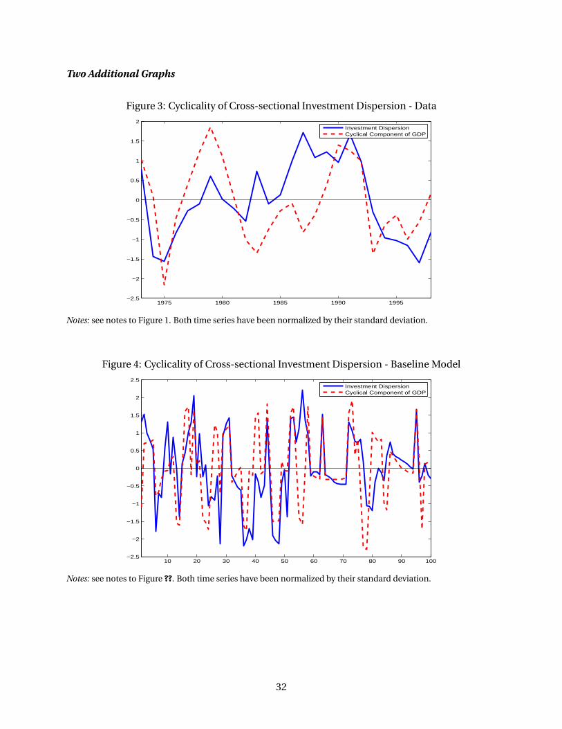
Two Additional Graphs

Figure 3: Cyclicality of Cross-sectional Investment Dispersion - Data

1975 1980 1985 1990 1995−2.5

−2

−1.5

−1

−0.5

0

0.5

1

1.5

2

Investment DispersionCyclical Component of GDP

Notes: see notes to Figure 1. Both time series have been normalized by their standard deviation.

Figure 4: Cyclicality of Cross-sectional Investment Dispersion - Baseline Model

10 20 30 40 50 60 70 80 90 100−2.5

−2

−1.5

−1

−0.5

0

0.5

1

1.5

2

2.5

Investment DispersionCyclical Component of GDP

Notes: see notes to Figure ??. Both time series have been normalized by their standard deviation.

32

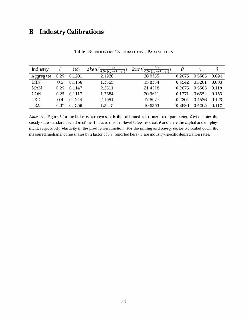
B Industry Calibrations

Table 18: INDUSTRY CALIBRATIONS - PARAMETERS

Industry ξ σ(ε) skew(ii ,t

0.5∗(ki ,t+ki ,t+1) ) kur t (ii ,t

0.5∗(ki ,t+ki ,t+1) ) θ ν δ

Aggregate 0.25 0.1201 2.1920 20.0355 0.2075 0.5565 0.094MIN 0.5 0.1156 1.3355 15.8334 0.4942 0.3201 0.093MAN 0.25 0.1147 2.2511 21.4518 0.2075 0.5565 0.119CON 0.25 0.1117 1.7684 20.9611 0.1771 0.6552 0.153TRD 0.4 0.1244 2.1091 17.6077 0.2204 0.4536 0.123TRA 0.07 0.1356 1.3315 10.6363 0.2896 0.4205 0.112

Notes: see Figure 2 for the industry acronyms. ξ is the calibrated adjustment cost parameter. σ(ε) denotes the

steady state standard deviation of the shocks to the firm-level Solow residual. θ and ν are the capital and employ-

ment, respectively, elasticity in the production function. For the mining and energy sector we scaled down the

measured median income shares by a factor of 0.9 (reported here). δ are industry-specific depreciation rates.

33