Investing in Lending Technology: IT

Spending in Banking∗

Zhiguo He, Sheila Jiang, Douglas Xu, Xiao Yin

Abstract

This paper investigates lending technologies in the banking sector after the arrival ofthe information age, by examining investment in information technologies (IT) by U.S.commercial banks. Given the distinctive nature of banks’ dealings with informationas they engage in lending activities, we link banks’ IT spending in various categoriesto different aspects of their lending technologies. Investment in communication IT isshown to be associated more with improving banks’ ability of soft information pro-duction and transmission, while investment in software IT helps enhance banks’ hardinformation processing capacity. By exploiting polices that affect geographic regionsdifferentially, we show that banks respond to an increased demand for small businesscredit (mortgage refinance) by increasing their spending on communication (software)IT spending. We also find an asymmetric impact of technological development on laboremployment in the banking sector.

Keywords: Information Technology, Small Business Lending, Mortgage Refinance,Communication Equipment, Software, Hard and Soft InformationJEL codes: G21, G51, J24, O32

∗He: Booth School of Business, University of Chicago and NBER, zhiguo.he@chicagobooth.edu; Jiang:Warrington College of Business, University of Florida, sheila.jiang@warrington.ufl.edu; Xu: WarringtonCollege of Business, University of Florida, douglas.xu@warrigton.ufl.edu; Yin: PhD program in Finance,Haas School of Business, University of California, Berkeley, yinxiao@berkeley.edu. We are thankful forvaluable comments from seminar participants at the Richmond Fed, University of Connecticut and Universityof Florida. Zhiguo He acknowledges financial support from the John E. Jeuck Endowment at the Universityof Chicago Booth School of Business. All errors are our own.

1 Introduction

Commercial banks have long relied on cutting-edge technology to deliver innovative prod-

ucts such as ATMs and online banking, streamline loan making processes, and improve

back-office efficiency. According to a 2012 Mckinsey Report, across the globe commercial

banks spend about 4.7% to 9.4% of their operating income on information technology (IT);

for comparison, insurance companies and airlines only spend 3.3 percent and 2.6 percent of

their income, respectively. This trend has accelerated at an unprecedented pace in recent

years, especially after the COVID-19 pandemic, as industry professionals often consider top

commercial banks to be more like “technology companies” than actual technology companies

by virtue of their enormous IT budgets.1 Recently, the impact of information technology on

the banking sector and financial stability has been a hot topic in policy discussions (Banna

and Alam (2021), Pierri and Timmer (2020)).

Although the financial services industry—especially the banking industry—is increasingly

becoming a tech-like business, the academic literature lags behind in understanding the

economics of IT spending in the banking industry. Which banks, large or small, have invested

more? How does IT spending affect banks’ lending technology and loan making? Our study

takes the first step toward understanding the basic pattern of these banking IT expenditures

and explores the connections and underlying mechanisms between these expenditures and

the core functioning of the banking system.

To place our research in the established banking literature, think about the information

transmission between a loan officer and a borrower, or across layers of loan officers within

a bank organization. As highlighted by Stein (2002), soft information tends to be more

effectively transmitted and thus lending decisions are more easily determined when a bank1For instance, this article shows that IT spending by most top banks, including JP Morgan, Bank of

America, Citi, Goldman Sachs and international leaders like Deutsche Bank and Barclays, exceeds 17%of their total operating costs, while Amazon and Alphabet devote 12% and 20% of their operating costsrespectively to IT. This article stresses that banks are still lagging quite a bit in their IT spending in absoluteterms, and cautions further that the above-mentioned IT spending numbers do not include compensationfor IT staff members.

1

has less hierarchical structure. The fast developing technologies in recent decades provide

more options for the banking sector to cope with such problems. Indeed, in recent years banks

have been observed to pay more attention to strengthening their internal communication

through the wide use of private branch exchanges and intranet installment.2 And technology

advances extend far beyond internal communication; for instance, the explosive big data

analytics market—which combines “hard” information like credit scores and other alternative

data—calls for automatic information processing as a pressing need for banks today.

Our study relies on a comprehensive dataset, the Harte Hanks Market Intelligence Com-

puter Intelligence Technology database, which has been used in the economics literature

(e.g., Bloom et al. (2014) and Forman et al. (2012)) for studying the economic implications

of technology adoption in the non-financial sector. Focusing on commercial banks, we are

the first—to the best of our knowledge—to analyze this dataset with detailed branch-level

information on detailed spending categories.

Section 2.2 explains in detail the four major categories of IT expenditure in the Harte

Hanks dataset—hardware, software, communication, services—in the context of the banking

industry. As we will explain shortly, our study focuses on two of these four categories. First,

Software includes desktop applications (e.g., Microsoft Office), information management soft-

ware, and risk and payment management software. By greatly improving the efficiency of

document assembly, digitization, information classification, these software products auto-

mate information processing through specialized programming and AI technologies and thus

improve both accuracy and processing speed.

On the other hand, Communication, which includes radio and TV transmitters, private

branch exchanges, and video conferencing, is defined as the network equipment that banks

operate to support their communication needs. For instance, a set of advanced communica-

tion equipment allow bankers to interact with their borrowers in a more effective way; and

private branch exchanges facilitate smoother exchanges of information and opinions within2For instance, a news article on Finextra reports the installment of intranet by First Citizens National

Banks.

2

the bank branching network.

In Section 3, we start our analysis by first documenting that IT expenditure in the

US banking sector has been growing rapidly over the last decade; for instance, average IT

spending as a share of total expenses has grown from nearly nil in 2010 to around 5% since

2015. A further examination across bank size groups reveals a somewhat different pattern

between small and large banks in terms of their time trends as well as the structure of

IT spending. The IT spending at large banks (asset size $10–250 billion) has been steadily

growing, while there is almost no growth in the smallest group (asset size below $0.1 billion).

Interestingly, medium-sized banks saw the fastest growth in their IT spending during 2010–

2014 but dramatically slowed down during 2015–2019; while mega banks (asset size above

$250 billion) only picked up their IT spending after 2015. In terms of the IT spending profile,

a noticeable distinction is that smaller banks consistently allocate a higher share of their IT

budget towards communication technology than larger banks do.

As we aim to achieve a better understanding of the formation of banks’ lending technol-

ogy during the information age, a natural yet important step is to examine the relationship

between banks’ investment in IT and their lending activities. Section 3.3 documents how

banks’ loan categories on balance sheets vary with their IT spending profiles. Among the

three large loan types in Call Report, we find that the shares in commercial and industrial

(C&I) loans and agricultural loans are positively associated with their communication spend-

ing, but uncorrelated with software spending, whereas the share of personal loans appears to

be positively associated with banks’ software spending, but not with communication spend-

ing. Furthermore, within C&I loans, small business lending stands out to drive the positive

association with communication IT spending; whereas within the personal loans, mortgage

refinance drives the positive association between personal loans and software spending. These

findings are robust at both bank and bank-county-year level.

Based on the above findings, we develop three main hypotheses in Section 4 linking the

nature of information in banks’ lending activities to their IT spending behaviors. Conceptu-

3

ally, we differentiate two fundamental types of bank lending technologies. The first heavily

relies on the gathering and augmentation of soft information from borrowers; in the context

of Berger and Udell (2002a), “relationship lending” is a concrete example of the first type.

The second fundamental type of lending technology, on the other hand, relies primarily on

the processing and quantification of hard information. “Transactions lending” in Berger and

Udell (2006), i.e., loans that are based on a specific credit scoring system and quantified

financial statement metrics, are standard examples of the second type.

For our first testable hypothesis, we posit that a demand shock of small business credit

will lead banks to invest more in communication technologies. This is because communica-

tion technologies—say video conferencing—not only enable banks to more effectively collect

soft information from small business borrowers (who often inhabit an opaque information

environment), but also allow for a smoother transmission of this otherwise hard-to-verify

soft information within a bank organization. Taking advantage of an arguably exogenous

demand shifter, we find that an increase in banks’ small business credit demand—due to a

higher ex-ante exposure of local counties to the policy shock exploited in our analysis—leads

to a positive and significant growth in banks’ communication spending, without much impact

on the bank’s software spending.3

The second testable hypothesis is that a positive demand shock for mortgage refinancing

should push banks to engage in more IT spending on software because software is particularly

useful for dealing with existing or readily accessible “hard” information (e.g., credit scoring

software utilized by banks when making refinancing decisions). To identify the causal rela-

tionship between a demand for “hard” information processing and banks’ software spending,

we construct a shifter to the mortgage refinance demand faced by banks across different

regions. Specifically, we utilize the cross-county variation in the interest payment gap of

outstanding mortgages due to the presence of a local mortgage rate gap—a higher interest3We construct our instrumental variable for the shock of small business credit demand based on “Small

Business Health care Tax Credit.” As a part of the Affordable Care Act, this program was enacted between2014 and 2015 and provided beneficial tax treatment specifically targeted at small business establishmentsin the US economy.

4

payment gap naturally implies a higher mortgage refinance demand by local households.

Thanks to this instrumental variable, which has been used in the literature (e.g., Eichen-

baum et al. (2018)), we show that a one standard deviation increase in mortgage refinancing

lent out by a bank leads to around 5% higher on average software spending intensity relative

to the sample average (due to its local exposure to high refinance savings), without any

significant impact on local banks’ communication spending.

Our last testable hypothesis concerns how investment in IT affects labor in the banking

industry, as development in information technologies offers more options for banks to per-

form “tasks” traditionally undertaken by employing human labor (Acemoglu and Restrepo

(2018)). Specifically, utilizing the county-level availability of land-grant colleges as an in-

strumental variable for local supply of IT-related employees, we find that banks operating

in counties with a more abundant supply of IT-related employees have significantly slower

software spending growth compare to those located in regions where the supply of IT-related

employees is relatively scarce. In contrast, we do not see such a difference in banks’ commu-

nication spending growth. Quantitatively, a one standard deviation increase in IT-employee

hiring growth results in an average of 5.13% slower growth in software spending as a share

of branch-level gross revenue. These results, which could be driven by a local wage channel,

indicate an important yet asymmetric impact of the development in information technologies

on the labor employment outcomes in the traditional banking sector.

Related Literature

Bank lending technology and the nature of information This paper is closely related

to the literature of relationship and transactions lending. Berger and Udell (2006) provide

a comprehensive framework of the two fundamental types of bank lending technology in

the SME lending market.4 A fundamental difference between these two types of lending

is related to the role played by information as highlighted by Stein (2002), who provides4Bolton et al. (2016) study the joint determination of relationship lending and transactions lending. They

find that firms that rely more on relationship banking are better able to weather a crisis than firms that relyon transactions banking, suggesting a higher capital requirement for relationship banks.

5

an explanation as to why soft information production favors an organizational structure

with fewer hierarchical layers and why banks cut their lending to small businesses after

consolidation. This notion that credible communication is essential for the production of

soft information is in line with our finding that spending on communication technology

facilitates the generation and transmission of soft information, while smaller banks tend

to allocate a higher proportion of their IT budget to communication compared with larger

banks.5

We contribute to this strand of the literature by linking information technology to

bank lending technology, especially on the distinction between soft information produc-

tion/transmission and hard information processing. We demonstrate causal linkages between

the different informational components in credit demand to banks’ endogenous decisions on

lending technology adoption.6 Although previous literature has shown how the credit sup-

ply will positively affect non-financial firms’ technology adoption or innovation (Amore et al.

(2013), Chava et al. (2013), Bircan and De Haas (2019)), it remains unknown how credit de-

mand associated of different informational natures will induce the banking sector to upgrade

their lending technologies. Establishing such causal relationship could help explain why

unbalanced development across different types of information technology could tilt banks’

lending towards or away from certain types of lending in the long run.

Information technology and the banking industry While the exact mechanism through

which information technology affects banks’ lending technology remains somewhat a black

box, the interactions between the development of information technology and the evolution

of the banking industry have been well explored in the literature. For instance, Hannan and5Along these lines, Liberti and Mian (2009) find empirically that greater hierarchical distance leads to less

reliance on subjective information and more on objective information and that more frequent communicationbetween information collecting agents and loan approving officers can mitigate the effects of hierarchicaldistance on information use. Paravisini and Schoar (2016) document that credit scores, which serve as “hardinformation,” improve the productivity of credit committees, reduce managerial involvement in the loanapproval process, and increase the profitability of lending.

6Hard and soft information components are never black and white. Berger and Black (2011) emphasizethat hard lending technologies often have both hard and soft information components, so large banks’comparative advantage in hard lending technology is dependent on the relative importance of the hardversus soft information components involved in the technology.

6

McDowell (1984) document that larger banks and banks in a more concentrated banking

industry are more likely to adopt automated teller machines. Stepping back into the twenti-

eth century, Berger (2003) shows that technological progress in both information technology

and financial technology led to significant improvement in banking services productivity and

quality. Petersen and Rajan (2002) document that development in communication technol-

ogy greatly increased the lending distance of small business loans, reflected in a relaxation in

the requirement that firms receiving credit in more distant areas need to have higher credit

score.7

The emergence of fintech is a signature result of recent developments in information

technologies.8 Our study aligns more closely with the angle addressing how the emergence of

fintech industry is affecting (or has affected) the traditional banking sector.9 While a common

theme of this research has mostly focused on examining how the emergent fintech industry is

affecting bank-fintech competition, in a process where traditional banks are largely viewed as

a passive player, and little attention has been paid to how banks are actively responding to

the emergence of this group of new challengers. Our paper makes the initial step in studying

whether and how the traditional banking sector is catching up with the penetrating fintech

industry through examining IT investment behavior in the U.S. banking sector.

Endogenous technology adoption and its real impact Recently, there has been a

large literature studying the endogenous adoption of IT across non-financial firms or geo-

graphical units and its impact on real economic outcomes, such as firm productivity, em-7There is also a vast theoretical literature on the interactions among information technology, banking

market competition and bank lending; see Freixas and Rochet (2008) for a review. Hauswald and Marquez(2003) analyzes how two dimensions of technological progress affect competition in financial services. Theyshow that although technological progress will lower the cost of information processing, it also implies lowerentry cost and higher competition. So the overall effect of technological progress on interest rates is mixed.More recently, Vives and Ye (2021) study how the diffusion of information technology affects competition inthe bank lending market and banking sector stability.

8Related works include but are not limited to Di Maggio and Yao (2020), Frost et al. (2019), Hughes et al.(2019), Stulz (2019), Fuster et al. (2019), Buchak et al. (2018), Jagtiani and Lemieux (2017), and Philippon(2020).

9Related research in this strand of literature includes Lorente et al. (2018), Hornuf et al. (2018), Calebe deRoure and Thakor (2019), Tang (2019), Erel and Liebersohn (2020), Aiello et al. (2020), Schnabl and Gopal(2020), and He et al. (2021).

7

ployment and local wages. This literature include McElheran and Forman (2019), Bloom

and Pierri (2018), Brynjolfsson and Hitt (2018), Akerman et al. (2015), Bloom et al. (2012),

Beaudry et al. (2010), Autor et al. (2003), Brynjolfsson and Hitt (2003).

In particular, to the best of our knowledge, our paper is the first to document that as in-

formation technology develops, banks with lower (higher) availability of IT-related employees

will accordingly invest more (less) in technology aimed at processing hard information pro-

cessing, without much impact on investment in communication technology, which primarily

helps soft information generation/transmission. These findings suggest that developments

in information technology could have an important yet asymmetric impact on labor employ-

ment in the banking sector.

2 Data and Background

We explain our main data sources in this section, together with detailed explanations of

various categories of IT spending.

2.1 Data Source and Sample

The data on banks’ IT spending comes from the Harte Hanks Market Intelligence Com-

puter Intelligence Technology database, which includes information on over three million

establishment-level IT transactions from 2010 to 2019 from conducting IT-related consult-

ing for firms.10 Harte Hanks collects and sells this information to technology companies,

who then use this information for marketing purposes or to better serve their clients. Firms

with IT spending information have incentives to report truthfully to Harte Hanks because

they also want to receive advice for better IT services in the future. This data set has been10One data issue is on how to allocate IT costs among branches the headquarter makes the purchase.

According to the data provider, in the case where the IT spending made by the headquarters of a bankis distributed to branches, such spending is reflected in the branch’s spending rather than in that of theheadquarters. Furthermore, by comparing the headquarters and branch spending scaled by revenue of thelargest 100 banks in our sample, we find no statistically significant difference between the IT spendingintensity at the headquarters and branches.

8

used in academic research in economics; leading examples include Bloom et al. (2014), who

study the impact of information communication technology on firms’ internal control, and

Forman et al. (2012), who study firms’ IT adoption and regional wage inequality.

Our paper focuses on commercial banks; to the best of our knowledge, we are the first to

analyze this data set with branch-level information as well as detailed IT spending categories

in the context of the banking industry. The sample consists of 1806 commercial banks in

the U.S. As shown in Figure A1, which displays the comparison between the total asset size

of banks in our sample and that of the overall banking industry in U.S. from 2010 to 2019,

our sample covers more than 80% of the U.S. banking sector in terms of asset size.

Our sample is more representative for large banks, as shown in Table 1 which reports

the coverage of our sample by bank asset size group. For three groups of banks with asset

size above $1 billion, the coverage in frequency and asset are both over 80%. However, for

small banks with size less than $100 million, our sample covers 14.45% (14.23%) of the total

number (assets) of commercial banks in the U.S. system.

Table 2 displays the summary statistics of banks’ IT spending. In our sample, the bank’s

total IT spending as a percentage of its net income ranges from 1.8% (25th percentile)

to 13.5% (75th percentile), suggesting a large variation across different banks. Median IT

spending as a share of net income is 5.1% (the 5.1% is calculated by using the observations

with positive net income), consistent with the 2012 survey by McKinsey reporting that

banks’ IT spending as a share of net operating income ranges from 4.7% to 9.4%.11

2.2 IT Investment Categorization

A major strength of our dataset is that it gives us a detailed decomposition of banks’

IT investments in four major categories specified by Harte Hanks: hardware, software, com-

munication, and services. We now provide detailed explanations for these categories, with

formal definitions given in 5(a) to 5(d) of Figure A4.11A screenshot of the report is in Appendix Figure A3.

9

Software is defined as software purchased from third parties. This could be packaged

or semi-packaged software delivered on CD and installed by the company, or offered on an

SaaS from a multitenant shared-license server accessible by a browser, or custom-created for

a company by third-party contractors or consultants. More specifically, the category of soft-

ware includes desktop applications, information management software, processing software,

ePurchase, risk and payment management software.

One representative example of desktop application is the Microsoft Office software pack-

age; these software products are easy to grasp by bank employees and allow employees to

conduct basic calculations and visualization of data that’s associated with lending business.12

Examples of processing software include Trapeze Mortgage Analytics, Treeno Software,

Kofax, eFileCabinet. The specialty of these software products lies in automatically pro-

cessing information from loan applicants’ paper document packets through specialized pro-

gramming and AI technologies, which greatly improve the efficiency in document assembly,

digitization, and information classification, which would otherwise be done manually by loan

officers. These software improve accuracy and shorten processing speed.

ePurchase software products allow banks’ customers to make fund transfers more easily

online and through mobile apps. Examples of ePurchase include Zelle and Stripe. For

instance, large banks (say BOA, CitiBank, and Wells Fargo) as well as smaller regional

banks (say First Tennessee Bank and SunTrust Bank) have joined the Zelle network, which

allows their customers to transfer funds across their bank accounts within seconds.

Risk management software provides on-going risk assessment after loans have been issued,

through augmenting borrowers’ repayment information as well as real-time industrial and

economic conditions. These software products, e.g. Actico, ZenGRC, Equifax, Oracle ERP,

allow banks to better monitor loans in progress. Other software products include security

trading systems and operating systems that are typically bundled with the specific software

products.12For example, on Mendeley.com, the job postings for loan officers or project managers by many banks

require applicants to be proficient with Microsoft Office.

10

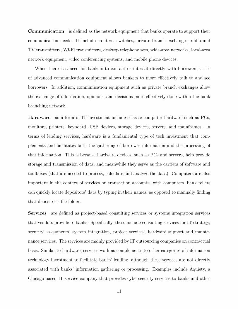
Communication is defined as the network equipment that banks operate to support their

communication needs. It includes routers, switches, private branch exchanges, radio and

TV transmitters, Wi-Fi transmitters, desktop telephone sets, wide-area networks, local-area

network equipment, video conferencing systems, and mobile phone devices.

When there is a need for bankers to contact or interact directly with borrowers, a set

of advanced communication equipment allows bankers to more effectively talk to and see

borrowers. In addition, communication equipment such as private branch exchanges allow

the exchange of information, opinions, and decisions more effectively done within the bank

branching network.

Hardware as a form of IT investment includes classic computer hardware such as PCs,

monitors, printers, keyboard, USB devices, storage devices, servers, and mainframes. In

terms of lending services, hardware is a fundamental type of tech investment that com-

plements and facilitates both the gathering of borrower information and the processing of

that information. This is because hardware devices, such as PCs and servers, help provide

storage and transmission of data, and meanwhile they serve as the carriers of software and

toolboxes (that are needed to process, calculate and analyze the data). Computers are also

important in the context of services on transaction accounts: with computers, bank tellers

can quickly locate depositors’ data by typing in their names, as opposed to manually finding

that depositor’s file folder.

Services are defined as project-based consulting services or systems integration services

that vendors provide to banks. Specifically, these include consulting services for IT strategy,

security assessments, system integration, project services, hardware support and mainte-

nance services. The services are mainly provided by IT outsourcing companies on contractual

basis. Similar to hardware, services work as complements to other categories of information

technology investment to facilitate banks’ lending, although these services are not directly

associated with banks’ information gathering or processing. Examples include Aquiety, a

Chicago-based IT service company that provides cybersecurity services to banks and other

11

firms; and Iconic IT, a New-York based IT service company that provides software and

hardware procurement, and installment and upgrade services.

2.3 Other Datasets

To supplement our study on banks’ lending technologies and banks’ IT investments, we

combine loan level information from multiple sources.

Bank Balance Sheet We obtain bank-level balance sheet information from Call Report.13

Total revenue of a branch is from Harte Hanks. Control variables constructed from Call

Report include Net income, Equity, and Deposits, all as a ratio of Assets. For bank-county

or bank-county-year analysis, we utilize information on banks’ revenues at the county level

from Harte Hanks. To guarantee the accuracy of this measure, we require that a bank’s

total revenue not be missing in that county and that the total number of employees at

a bank’s branches in this county is not missing in the Harte Hanks database when it was

surveyed. To construct the key left-hand side variables “IT spending/Revenue,” we aggregate

all branches’ spending in a specific category of bank i in county c in year t, and scale it by

the aggregated revenue of all branches of that bank in that county. The control variable

“Revenue per employee” is at bank-county-year level, with total revenue and total number of

employees both from Harte Hanks. When using this control variable for bank-level analysis,

we aggregate revenue and employees at the bank level across the nation and calculate this

ratio.

Loans and Local Characteristics We obtain syndicated loan information on the fre-

quency of a bank acting as lead bank in syndicated loan packages from LPC Dealscan. Small

business loan origination data are from the Community Reinvestment Act (CRA), which is

at the bank-county-year level covering the sample period of 2010–2019. Mortgage refinance

information is available in Home Mortgage Disclosure Act (HMDA) from 2010–2019. When13To merge Call Report data with the Harte Hanks data, we merge by bank name using levenshtein

distance (similar to the method used in Lerner et al. (2021)) after dropping suffixes such as corporation orinc. And we require a matching score above 90%.

12

constructing an instrumental variable that serves as a demand shifter, we download the av-

erage mortgage interest rate at the county level before 2010 from Freddie Mac. County-level

variables are matched by FIPS.

3 Empirical Patterns of Banks’ IT Spending

We start our analysis by reporting some basic statistics of banks’ investment in IT over

the last decade in the U.S. economy and explore how a bank’s IT investment relates to its

size. We then show that banks’ IT investments are closely related to their lending activities,

by examining how the profiles of banks’ IT investments vary when banks have different

specialization in loan types (e.g., commercial loans versus personal loans).

3.1 Time Trends of Banks’ IT Investment

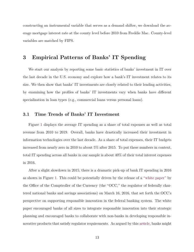
Figure 1 displays the average IT spending as a share of total expenses as well as total

revenue from 2010 to 2019. Overall, banks have drastically increased their investment in

information technologies over the last decade. As a share of total expenses, their IT budgets

increased from nearly zero in 2010 to about 5% after 2015. To put these numbers in context,

total IT spending across all banks in our sample is about 40% of their total interest expenses

in 2016.

After a slight slowdown in 2015, there is a dramatic pick-up of bank IT spending in 2016

as shown in Figure 1. This could be potentially driven by the release of a “white paper” by

the Office of the Comptroller of the Currency (the “OCC,” the regulator of federally char-

tered national banks and savings associations) on March 16, 2016, that set forth the OCC’s

perspective on supporting responsible innovation in the federal banking system. The white

paper encouraged banks of all sizes to integrate responsible innovation into their strategic

planning and encouraged banks to collaborate with non-banks in developing responsible in-

novative products that satisfy regulator requirements. As argued by this article, banks might

13

have gained more freedom thanks to this white paper and have been more actively investing

in information technology in order to better catch up with fintech development.14

Indeed, through examining how this time trend of banks’ IT investments moves to-

gether with the fintech presence in a local economy, we find evidence suggesting a potential

“catching-up” behavior of the traditional banking sector. Figure 2 plots the average IT

spending over years as a share of revenue by local commercial banks, for geographic regions

featuring high and low fintech presence respectively.15 While IT spending by banks in both

groups share a common upward trend, the group with high fintech presence increases their

IT spending at a faster rate than the one with low fintech presence.

As another important input in banks’ lending technology investment, banks’ IT-related

labor hiring—which used to be the major form of lending technology investment before the

information age—is also of interest to our study. Figure 3 compares IT spending between

banks with high and low levels of IT-related labor employment.16 We find that banks with

low IT-related labor employment have experienced faster growth in IT spending over the

last decade, an interesting observation that we come back to in Section 4.4.

In addition to the time dynamics of the IT spending of U.S. commercial banks, another

equally important dimension of our analysis is the structure of these investments in infor-

mation technology. Table 2 reports summary statistics on the detailed structure of banks’

IT spending profiles. In particular, we report how banks’ investments in IT are distributed

across different categories as defined in Section 2.2. By size, software and services are the

largest among all categories of IT spending, each constituting 33% of total IT budget. Hard-

ware constitutes about 17% of total IT budget, and communication is on average 9%. In

our sample, an average bank has a storage size of 3.52PB (3604.5 TB) and 133 IT-related14This article by McKinsey documents a fintech IPO boom as well as a fintech investment boom by venture

capitalists since 2016.15County-level fintech presence measure is based on “Fintech lending share in local mortgage market”

proposed in Fuster et al. (2019), and we define high (low) fintech presence regions to be counties withabove-median (below-median) of the fintech lending share.

16In this comparison, banks with high and low level of IT-related labor employment are defined as bankswhose IT employee share (as a fraction of total employee) is above the 80th percentile and below the 20thpercentile, respectively.

14

employees.

3.2 Bank IT Spending across Bank Size

We now examine how IT spending varies across different bank groups, by conducting the

same set of analyses as in the last section, but for different banks size groups. Table 2 reports

the summary statistics of banks’ IT spending and Table A2 reports the summary statistics

by bank size. Overall, we find that larger banks tend to make more IT investment as a share

of noninterest expenses than smaller banks do. As can be seen in Table A2, banks with total

assets of less than $0.1 billion have an average IT/revenue ratio of 1.5%, whereas banks with

asset size in the range of $1–$10 billion and banks in the range of $10–$250 billion have an

average IT/revenue ratio of 4.3% and 4.5% respectively.

Panel A of Figure 4 displays the time trend of banks’ IT investments by each bank size

group. Overall, an upward trend in IT spending as a share of total non-interest expense is

observed in all bank size groups.17 Despite this common upward trend over the past decade,

there are also some noticeable differences in the detailed dynamics across different bank size

groups. Among the five size groups, IT spending in large banks (asset size $10–250 billion)

has been steadily growing, while there is almost no growth in the smallest group (asset

size below $0.1 billion). Interestingly, medium-sized banks (banks in asset size bins $0.1–1

billion and $1–10 billion) saw the fastest growth in their IT spending during 2010–2014 but

dramatically slowed down during 2015–2019. In contrast, mega banks (asset size above $250

billion) only picked up their IT spending after 2015.

Another noticeable feature revealed by cross-size summary statistics is that smaller banks

tend to allocate a higher fraction of their IT budget towards communication technology than

larger banks do, while there are no significant differences in the software spending as a share

of total IT spending across asset groups. (We will come back to this point in Section 4.2.)

As shown in Panel B of Figure 4, the average communication/total spending ratio is 15.9%17The magnitude of IT budget as a share of noninterest expenses in this figure is also in line with Hitt

et al. (1999). In their survey banks’ IT spending could be as high as 15% of noninterest expenses.

15

for banks with assets less than $0.1 billion; this ratio monotonically decreases with bank

size. A full comparison of the spending on communication and software (as a share of total

IT spending) across different bank size group is shown in Table A2.

3.3 Bank IT Investment and Bank Lending

We now perform a comprehensive study on the relationship between banks’ IT invest-

ments and their (relative) specialization in three major types of loans: commercial and

industrial (C&I) loans, personal loans, and agricultural loans. Lending to different types

of borrowers often involves distinct ways of dealing with relevant information, due to the

different characteristics of borrowers. As a consequence, if banks specialize in different types

of loan making, one should expect them to differ in their IT investment profiles.

As a first step, we run the following bank-level regression (we leave the more granular

bank-county level analysis for later):

Type S IT SpendingRevenue i,10−19

= αi + βType L loanTotal loan i,10−19

+ γXi + εi. (1)

Here, i refers to bank and the outcome variable of interests is Type S IT spendingTotal IT Spending i,10−19

, which

is the average investment intensity in a specific type of IT spending as a share of bank i’s

revenue between 2010 and 2019. The main explanatory variable Type L loanTotal loan i,10−19, which

captures bank i’s loan specialization, is measured by the average share of a specific type of

bank i’ loan relative to its total loan size. Control variables include net-income scaled by

total assets, total deposits scaled by total assets, revenue per employee, total equity scaled by

total assets and total salaries scaled by total assets. All of the control variables are measured

over the ten-year average between 2010 and 2019 at the bank level.

Table 3 reports the estimation results of the regression (1) for C&I loans with the detailed

regression outcome including control variables and fixed effects, while for exposition purpose

Table 4 only reports the key regression coefficients (i.e., those of specific IT spending shares)

16

for C&I loans, personal loans, and agricultural loans using the same methodology.

A. Commercial and Industrial (C&I) Loans

Table 3 shows the association between C&I loans and different types of banks’ IT bud-

gets. Overall, our findings suggest that specialization in C&I loans is most positively and

significantly associated with banks’ spending in communication technology. A one standard

deviation increase in loan portfolio share allocated to C&I loans predicts a 0.053 standard

deviation increase in communication budget as a share of total revenue; in dollar terms, this

corresponds to an average of $0.14 million spending on communication.

A higher degree of specialization in C&I loans also predicts more spending on hardware,

although the magnitude is slightly smaller than that predicted for the communication budget.

On the other hand, the coefficient of software spending is insignificant.

Within C&I Loans In the next step, we decompose C&I loans into “Small Business

Loans,” as measured by a bank’s small business lending reported in CRA, and “Other C&I

loans.” Rows 2 and 3 of Table 4 illustrate how small business loans are compared to other

C&I loans in terms of their association with banks’ IT spending. while a higher share of

small business loans in a bank’s loan portfolio is positively and significantly associated with

the bank’s communication spending, small business loan share is negatively related to the

bank’s software spending. On the other hand, “other C&I loans”—presumably loans to

large firms—are positively associated with software spending, but not with communication

spending.

Row 4 of Table 4 further investigates a special type of loan (or lending form)—syndicated

loans, in which being a frequent lead bank versus playing more of the role as participant

banks. We postpone a more detailed discussion about this comparison to Section 4.2, after

we lay out a conceptual framework to think about the distinctive economic meanings of

different categories of IT investment in banking.

B. Personal Loans

17

The second major category of loan type we examine includes personal loans and mort-

gages. Row 5 of Table 4 reports the associations between specialization in personal loans/mortgages

and banks’ IT spending. Contrary to commercial and industrial loans, a higher share of loan

portfolio allocated to personal loans and mortgages appears to predict more spending on

software only. Quantitatively, a one standard deviation increase in loan portfolio share of

personal loans and mortgage (about an increase of 7 percentage points) predicts 0.045 stan-

dard deviation increase in software budget as a share of total revenue, or an average of $0.65

million more spent on software per year. On the other hand, a higher personal and mort-

gage loan share does not have qualitatively significant predictive power on communication,

hardware, or services budgets.

Within Personal Loans Paralleling our analysis within C&I loans, we also decompose

personal loans and mortgages into two subcategories: mortgage refinancing and everything

else. As shown in row 6 and row 7 (and compared with row 5) of Table 4 mortgage refinancing,

in particular, is positively associated with banks’ software spending within the broad category

of personal loans (including mortgages). When we study the economic meanings of banks’

IT spending in Section 4, this finding motivates us to pay particular attention to mortgage

refinancing as a specific type of lending activity in which the processing of hard information

plays a critical role.

Additionally, the abundance of mortgage data allows us to gain further insights about the

following important aspect of lending activities: originating a new loan versus refinancing

an existing loan. The result is reported in Row 8 of Table 4, and we postpone more detailed

discussion to Section 4.3.

C. Agricultural Loans

Finally, we examine the association between agricultural loan specialization and banks’

IT spending profiles. As shown in row 9 of Table 4, a higher proportion of agricultural loans

in a bank’s loan portfolio is positively associated with its communication spending. A one

standard deviation increase in allocation towards agricultural loans (4.8 percentage points

18

higher) is associated with a 0.056 standard deviation increase in communication budget, or

an average of $0.11 million more spending on communication per year.

4 Economics of Banks’ IT Investment

Having demonstrated the basic patterns of IT investment in the U.S. banking sector and

its interaction with various factors, we now move on to a deeper question: What are the

economics behind these banks’ IT spending, and in particular, how can they be related—and

contribute—to the development of banks’ lending technology? The answers to these ques-

tions are relevant for a better understanding of how banks develop their lending technologies

in the information age.

In Section 4.1, we provide a conceptual discussion of how banks’ lending technology

during the information age can relate to their investment in information technologies. We

then present some motivating evidence, which offers certain clues about the economics of IT

spending in banking, based on which we formalize several testable hypotheses.

4.1 Bank Lending Technology and Information

What is a bank’s lending technology? While the answer likely depends on the exact

definition of “technology,” a bank’s lending technology could largely be viewed as the bank’s

ability to deal with information regarding its borrowers. If one can map different types of

IT investment into different dimensions of banks’ lending technology, then we should expect

banks to allocate their IT spending differently according to the type of credit demand they

face.

The linkage between the role played by information that facilitates banks’ lending ac-

tivities and banks’ lending technology in the information age is important yet unexplored.

Broadly speaking, in conducting their lending businesses, banks engage in two types/stages

of activities regarding their borrowers’ information: information production/transmission

19

and information processing. More specifically, information production/transmission, which

is broadly related to soft information in Stein (2002), refers to the stage in which informa-

tion on borrowers needs to be created or gathered and then relayed to the hands of those

who later make decisions based on this information, whereas information processing, which

is broadly related to hard information in Stein (2002), is more about the stage in which

existing (or readily available) information on borrowers needs to be properly utilized by the

lender for more efficient decision making.

4.2 Communication Technology and Soft Information

Let us start with information production/transmission. When faced with borrowers

lenders have never dealt with or borrowers whose information structure is relatively opaque,

the first thing they often need to do is to communicate with borrowers, so that they can

at least sketch a picture of the borrower with whom they can later examine in detail. Such

communications are often essential as the first step in allowing the lender to gather infor-

mation about their borrowers, either through talking to them face-to-face, or from seeing

borrowers’ projects for themselves.

Once this first-hand information about borrowers has been gathered, which often can be

quite subjective and thus difficult to convey to others, effective transmission of the gathered

information within the lending organization can be another crucial factor affecting lending

efficiency. This problem associated with the credible transmission of hard-to-verify infor-

mation within an organization has been recognized in previous studies (e.g., Stein (2002)).

Efficient internal communication and exchange is particularly important when the relevant

information is relatively soft, which is less objective and often harder to verify by someone

who is not the first-hand collector of the information.

One concrete example of how communication technology can help in the two aforemen-

tioned dimensions is video conferencing, which has become an important method for banks

to communicate with borrowers and customers during the past decade. In the past, banks

20

opened new account openings, originated loan, and resolved problems through in-person

visits to the brick-and-mortar branches, but they now use video conferencing technology as

it makes the direct—yet virtual—contact between loan officers and borrowers more timely

and cost saving.18 Moreover, video conferencing among the employees within banks has

also been welcomed by the banking sector for its advantage in facilitating effective internal

collaboration.19

Small Business Lending The lending to small business borrowers is one concrete example

of such a situation. Sahar and Anis (2016) document that in the context of lending to small-

and medium-size enterprises, direct contact with borrowers and frequent visits from loan

officers to the borrower allow loan officers to collect and produce soft information. Agarwal

et al. (2011) highlight that soft information, such as what the borrower plans to do with the

loan proceeds, is always the product of multiple rounds of interactions between the lender and

the borrower.20 Finally, since smaller banks overall issue more loans to small businesses than

larger banks do (e.g., Berger and Udell (2002b), Berger and Udell (2006), Hanson and Stein.

(2017)), this link between soft information generation and communication technology helps

explain why small banks tend to allocate more of their IT budget toward communication

spending as shown in Panel B of Figure 4.

Mortgage Initiation The production and transmission of soft information is not only

important from the angle of lenders, but also crucial from the perspective of borrowers,

especially in the context of mortgage initiation. An industry report shows that 90% of home

buyers, especially first-time home buyers, cite that they want to directly speak with a loan

officer. According to a recent article, Wells Fargo—after spending $500 million on digitizing18See a real-world example of the communication tool “Liveoak” designed for banking services.19See this article from Bankingdive for a detailed description of how video conferencing helps within-bank

communication.20The mapping between communication technology and soft information production is also reflected in

the relation between whether a bank serves lead banks frequently in loan syndications and its various ITspending, as shown in Table 4. The nature of interactions between lenders and borrowers differs if the lenderis a lead bank as opposed to participant banks: being a frequent lead bank requires frequent communication,reporting, coordination among borrowers and peer lenders.

21

mortgage experiences—admitted that “73% of home buyers wanted assurance that they could

speak with a real person through the process.” Mobile phone devices, desktop telephone

sets, Wi-Fi transmitters, and video conferencing devices are all important communication

infrastructure and ensure communication between borrowers and lenders for the generation

of soft information.21

Lead versus Participant (in Syndicated Loans) The syndicated loan market provides

a special environment to explore the relationship between communication technology and

soft information production. In syndicated loan lending, the nature of interactions between

lenders and borrowers differs drastically if the lender is a lead bank as opposed to being a

participant bank (Sufi (2007), Ivashina (2009)). Lead banks are mandated by borrowers to

acquire other lending participants, conduct compliance reports, and negotiate loan terms.

After the loan is issued, they also have the responsibility to conduct monitoring, distribute

repayments, and provide overall reporting among all lenders within the deal. In this regard,

lead banks’ job performing involves significantly heavier effort in information generation

and sharing as well as coordinating negotiations than that of a participant bank. In short,

effective communication plays a more central role in the functioning of lead banks than that

of participant banks.

The above conceptual difference between the roles played by lead banks and participant

banks naturally leads us to empirically examine whether the frequency with which a bank

participates in syndicated loans as a lead arranger can predict the bank’s IT investment

behavior, with the regression framework in Eq. (1) in Section 3.3. As shown in Table 4 row

4, a bank’s investment in communication technology exhibits a strong positive association21Not only does communication infrastructure help soft information generation at the loan origination

stage, but it also greatly enables lenders to closely monitor borrowers’ business conditions after the loanis issued, especially for information that is not directly observable or verifiable. A concrete example isagricultural loans; we have shown toward the end of 3.3 that agricultural loans are positively associated withcommunication technology investment. Indeed, effective monitoring of agricultural loans involves a goodestimate of farmers’ income and riskiness; but these are dependent on observing what is going on at thefarm—(e.g., are there pests or floods? is the weather normal?). Traditionally farms are monitored throughfrequent in-person visit to the farmland by loan officers. With advances in technology, more and more ofthis monitoring relies on video conferencing and even satellite image generation and transmission. See thisarticle describing the difficulty of monitoring agricultural borrowers faced by traditional lenders.

22

with the frequency of that bank serving as lead bank in syndicate loans, whereas a negative

association emerges between the bank’s software spending and its frequency serving as a lead

bank.

We hence propose the following hypothesis as to how banks’ investments in IT can be

mapped to their lending technology development. We will examine their causal relationship

in our later analysis.

Hypothesis I

Banks’ investments in communication IT are more associated with improving their abil-

ity to produce and transmit soft information. Specifically, in the context of small business

lending, banks will increase their spending on communication technology given an increase

of credit demand from small business borrowers.

4.3 Software Technology and Hard Information

We now move to information processing. Once information has been produced (by the

lender itself) or is readily accessible (via the third party), the next concern for the lender

is how to most efficiently utilize this information to make wise decisions. In the context of

credit allocation, banks need to be able to properly evaluate the creditworthiness of their

borrowers to determine loan amounts and rates. More specifically, when banks are faced with

borrowers whose information structure is relatively transparent or borrowers they already

have some knowledge about from previous interactions, lending decisions simply boil down

to efficient utilization and processing of the available information.

Accurate evaluations of borrowers’ credit risk often require complicated modeling and

simulations, which are often impossible without the support of sophisticated software tools.

In terms of facilitating lending activities, software is particularly useful for dealing with

existing or readily accessible “hard” information. Banks have actively adapted new software-

based technologies to store, organize, and analyze large chunks of loan applicants’ data, or

23

data augmented by other software. In this regard, investing in software can greatly help

banks to more promptly and accurately process the available information so that they can

make their lending decisions in a more efficient and reliable way. By contrast, several decades

ago all credit application information had to be stored on paper application forms, then

reviewed and processed manually by loan officers.22

From the banks’ perspective, software differs from communication technology in that com-

munication devices can facilitate the gathering and dissemination of information, whereas

software is more targeted at utilizing information that is readily available at hand.23 Because

of this difference, software as a category of banks’ IT budgets should be more relevant in

dealing with loans that primarily involve the processing and assessment of existing informa-

tion that is relatively “hard.” In practice, a specific form of software technology product is

the credit scoring software utilized by banks when making refinancing decisions. Some con-

crete examples of these credit scoring software include SAS Credit Scoring, GinieMachine,

and RNDPoint.24

Refinancing versus Origination (of Mortgage Loans) The discussion above suggests

that software IT should help greatly in refinancing existing loans as opposed to originating

new loans. Recall Section 3.3 analyzed the relationship between IT spending and banks’ loan

specialization; there, we find mortgage refinance stands out as a special type of loan that

appears to be particularly strongly associated with banks’ spending on software, as shown

in rows 6 and 7 of Table 4. To sharpen our understanding of the role played by software

in lending technology, we move one step further and conduct a similar analysis within the

mortgage lending business, by splitting mortgage business into mortgage origination and22For example “nCino” is operating system software that allows financial institutions to replace manual

collection of loan/account applications with automated and AI based solutions. “Finaxtra” and “Turnkey”are both comprehensive loan origination systems that offer solutions for the whole lending process.

23This difference also explains why fintech companies, who often serve as the suppliers of new bankingsoftware products, have expanded dramatically in the mortgage refinance market (e.g., Fuster et al. (2019),Seru (2019).)

24To use these software, banks usually just need to import available demographic and historical informationon borrowers, then the software calculates credit scores and conducts statistical tests for robustness using AIand machine learning methodologies, which save banks from tedious manual work and quicken the processing.

24

mortgage refinancing. We find that if a bank is a frequent “refinance” lender in the mortgage

market versus serving as an originator, which is measured by the percentage share of refinance

loans issued by the bank within its total mortgage lending in the HMDA data, the bank

also tends to spend more on software. The detailed results are reported in row 8 of Table

4. Finally, as expected, contrary to the positive significant association between software

spending and mortgage refinance, communication spending shows no correlation with activity

in mortgage refinance business.

Motivated by these findings, we propose and test the following hypothesis relating soft-

ware IT spending and hard information processing in commercial banks. Note, this hypoth-

esis is also consistent with the recent literature showing that fintech expansion is particularly

pronounced in the refinancing segment of the mortgage, auto loan, and student loan markets

(Drechsler et al. (2016)), as fintechs typically rely on readily available hard information.

Hypothesis II

Banks’ investments in software IT is more associated with improving their capability to

process hard information. Specifically, in the context of mortgage refinancing, banks are

likely to increase their spending on software IT when facing an increased credit demand for

mortgage refinancing purposes.

4.4 Labor Employment and Bank IT Investment

In addition to these two aspects of banks’ lending technologies and their relation to banks’

investments in IT, we also pay attention to a third dimension in understanding the economics

of how banks develop their lending technologies: the labor and employment in the banking

sector. In tandem with the widespread application of automation and artificial intelligence,

there has been ongoing debate about how this technological progress might impact the de-

mand for a human workforce. In the context of banking, if we treat banks’ labor employment

as a traditional input that deals with information production and information processing,

25

one question naturally arises: How would the adoption of new technology that deals with

information production/processing impact the job security of these bank employees? In par-

ticular, will banks’ investments in IT substitute out or complement bank employees who

perform information related tasks?

Given the complicated nature of interaction between IT-related employment and software,

together with rich economic forces at play (say factor prices), it is unclear a priori if we should

expect these two to be substitutes or complements. However, because generating new and

soft information would still have to rely (at least to some degree) on human labor, there is

much less substitution/complementarity between IT-related employment and communication

technology investment.

We have presented some empirical patterns that offer preliminary answers to both ques-

tions. Recall that we have learned from Figure 3 that banks with lower IT-related labor

hiring tend to have a higher growth rate in their total IT spending. Figure 5 further ex-

amines communication spending and software spending separately, and shows that the time

trend pattern documented in Figure 3 is mainly driven by banks’ spending on software

technology—not communication spending at all.

Therefore the data seem to suggest that, while indeed there is no relation between IT-

related employment and communication spending, there is a substitution effect between

IT-related employment and software spending in the banking industry. This could be driven

by many possible mechanisms: for instance, superior computing power and algorithmic

calculation would enable IT to effectively take over the task of processing relatively hard

information. We summarize this section by developing the following hypothesis, which again

will be formally tested in Section 5.3.

Hypothesis III

Banks’ adoption of information technologies has an asymmetric relationship with banks’

IT related employment. Specifically, i) investment in software IT is a substitute for banks’

IT-related employment, and therefore, banks tend to increase (decrease) their spending on

26

software IT when the supply of IT-related labor is scarce (abundant); yet ii) no such sub-

stitution effect exists between banks’ investment in communication IT and their IT-related

employment.

5 Empirical Designs and Tests

In this section, we exploit policies that affect geographic regions differentially to identify

the causal relationships highlighted in the hypotheses developed in Section 4.

5.1 Soft Information Production and Bank IT Investment

We first focus on Hypothesis I, which posits that banks should invest more in their

communication technology when faced with rising demand for credit that relies heavily on the

production/transmission of soft information. One typical example for such soft information–

driven credit is small business lending.

Soft information production plays a critical role in the small business lending sector

(Berger and Udell (2002a), Liberti and Petersen (2018)). Small business loans refer to

a special type of bank loan where banks mainly deal with young and opaque firms who

often have only limited credit history; Section 3.3 has shown a positive correlation between

specialization in small business lending and banks’ spending on communication technology

(Table 4, row “C&I loans”). Following this logic, we regard increased credit demand from

small business borrowers as a demand for more intensive production of soft information. The

goal of our identification analysis in this section is then to establish a causal relationship

between a higher demand for credit from small business borrowers and an increase in banks’

spending on communication technology.

Our identification strategy relies on an event-driven credit demand shock that hits the

U.S. banking sector heterogeneously across different regions in terms of small businesses’

credit demand. This feature allows us to extract and utilize variations that come from banks’

27

arguably exogenous exposures to such credit demand shocks. To motivate our approach, we

first present a set of scatter plots displaying banks’ IT investment patterns and lending

technology adoptions when they operate in different economic environments. The two upper

panels in Figure 6 display correlations between banks’ IT investments and the share of small

business in local counties. There, we see that a greater presence of small businesses (as

measured by establishment with ≤ 5 employees) in a local county is strongly positively

correlated with communication spending intensity of banks operating in the county, but not

with software spending.

Constructing Shifter in Small Business Credit Demand We utilize a special program

called the “Small Business Health Care Tax Credit” in the Affordable Care Act enacted

between 2014 and 2015, which was aimed at encouraging small businesses to provide health

care coverage to their employees. The program offers tax credit to small business employers

who pay health insurance premia on behalf of employees. To qualify for the tax credit, the

employer needs to (1) have 25 or fewer employees; (2) pay average wages less than $50,000 a

year per full-time equivalent; (3) pay at least 50% of its full-time employees’ premium costs;

and (4) have provided a health plan to employees that is qualified under the SHOP program

coverage requirements.25

There are many reasons for why the launch of this program could boost local small

businesses’ credit demand.26 For instance, small business owners who had not provided their

employees health coverage before the availability of the program might now be able to borrow

from banks and fund their working capital. What is more, with the tax credit subsidized for25See the guidance here directing to the introduction of the policy. According to the IRS, small business

employers should apply for the tax credit by filling in Form 8941. The tax credit can be carried backwardor forward to other tax years. Also, since the amount of the health insurance premium payments is morethan the total credit, eligible small businesses can still claim a business expense deduction for the premiain excess of the credit, which means both a credit and a deduction for employee premium payments. Smallbusinesses receive credit on a sliding scale. The smaller the employer, the bigger the credit. The tax creditis highest for small companies with fewer than 10 employees who receive an average annual salary of $25,000or less.

26Previous literature in economics has documented increases in labor demand, firm expansion, productivitygrowth, etc. after the implementation of corporate tax cuts or the launch of subsidies (Cerqua and Pellegrini(2014), Rotemberg (2019), and Ivanov et al. (2021)).

28

them, small businesses could potentially initiate desired expansion and development projects

from which they had previously been financially constrained.

While the implementation of this program tends to shift up credit demand from small

business borrowers universally across the U.S. economy, the exposure to this credit demand

shock may vary substantially across different regions, depending on their pre-event charac-

teristics. In particular, the number of qualified establishments at (or right before) the event

date, which features substantial variation across different counties, is a key determinant for

rising credit demand from small business borrowers in the local area.27 Such variation in

the pre-event number of qualified establishments can thus help us isolate variations in small

business credit demand across regions; since the policy only explicitly targets small busi-

nesses, its impact on other types of credit demand would be relatively limited or at least less

direct.

Empirical Design: 2SLS Regression Following our discussion above, we run the fol-

lowing 2SLS regression which uses “Qualified Small Businesses” (QSB) in 2013 as an instru-

mental variable of the local county’s exposure to the program:

∆ ln(CRA)i,c,post = µi + µ1 ln(1 + QSB)c,pre + µ2Xi,c + εi,c

∆ ln ITi,c,post = αi + β ∆ ln(CRA)i,c,post + γXi,c + εi,c.(2)

The first equation in Eq. (2) is the first-stage regression. The outcome variable ∆ln(CRAi,c,post)

is the change in the logarithm of bank i’s small business loans in county c in the three-year

time window after the program compared to its small business loans in the same county

three years before. The instrumental variable ln(1 + QSB)c,pre is the logarithmic of the to-

tal number of small businesses with fewer than 20 employees in 2013 before the policy shock;

due to data limitations we pick the cut-off “20,” as opposed to “25” as specified by the27Qualified establishments are small businesses with fewer than 25 employees, per the program’s stipula-

tions.

29

program.28 In the second stage, we regress ∆ln ITi,c,post, which is the change in logarithm

of a specific type of IT spending of bank i in county c after the program implementation

compared with before, on the fitted value from the first stage. In both stages, X represents

a vector of control variables that includes the bank fixed effect together with several bank-

county-level control variables. We have included the total number of establishments in 2013,

which controls for the total local credit demand (not just from small businesses).29

Estimation Results We report the estimation results of (2) in the first three columns of

Table 5. Column (1) shows the regression in the first-stage regression, and columns (2) and

(3) show results of the second stage.

Column (1) shows a strong first stage result with an F -statistic of 15.18, which is well

above the conventional threshold for weak instruments (Stock and Yogo (2005)). As reported

in columns (2) and (3), we find no significant response in banks’ software spending after

the program launch, but there is a positive and statistically significant response in banks’

communication investment across counties. In particular, banks who saw a one standard

deviation higher growth in their small business loan making, due to the higher shock exposure

of the counties in which they operated, experienced a 0.0745 standard deviation higher

growth in their communication spending. This translates to a 26% higher communication

spending, or an average of $67,830 more per year, compared with banks located in other

lower exposure counties. Note, our estimation includes bank fixed effects, so the above

result applies to within-bank, but cross-county variations.

Comparison: OLS Estimates To gain more insights about our 2SLS estimates, we also

compare them to the estimates from the OLS regression, with results reported in Columns28The “County Business Pattern” database provides categorization of small businesses sizes (number of

employees) based on the following cut-off; less than 5, 5-9, 10-19, 20-49, 50-99, 100-249, 250-499, 500-1000,more than 1000. We chose the closest cut-off, which is “fewer than 20.”

29The main control variable is “Revenue per Employee” at the bank-county level. The total revenue isat bank-county-level from Harte Hanks, and total number of employees is from Harte Hanks. County levelcontrol variables include the labor force, population growth rate, and total number of establishments.

30

(4)–(5) of Table 5:

∆ ln(IT)i,c,post = αi + β × ∆ ln CRAi,c,post + µc + γXi,c + εi,c. (3)

Qualitatively, OLS estimates are similar to those obtained from the 2SLS method: within

a bank, its branches in counties seeing a higher growth rate in small business loans invest

more in communication than other branches, but not in software spending.

Quantitatively, the magnitudes of the OLS coefficients are significantly smaller. One

potential explanation for such a downward bias in OLS estimators could be the following

“omitted variable” problem, in which counties with faster growth in small business loans

are those with even faster growth in some unobservable economic variables—say, mortgage

demand—that drives local banks to spend less on communication. More specifically, if

mortgage demand is correlated with demand for small business loans, and if banks have

a fixed amount of IT budget each year, then they will allocate more IT spending—say,

software—to cater to mortgage demand. The omitted-variable problem then leads the OLS

estimator to underestimate the responsiveness of communication spending towards small

business loan demand. The cross-region shifter constructed above based on the tax policy

targeting only small businesses thus allows us to isolate the variation in small business credit

demand from that of other types of credit.

5.2 Hard Information and Bank IT Investment

In this section, we identify the causal linkage between credit demand that requires in-

tensive processing of hard information and banks’ investments in software technology, which

concerns Hypothesis II in Section 4.3. By definition, “hard” information refers to the type of

information that is existent, can easily be quantified, and does not require further verification.

In terms of lending, loan origination and refinancing provide an ideal setting to investigate

the relationship between “hard” information and banks’ lending technology investments.

31

Mortgage refinancing is a special type of loan that primarily involves processing existing

information, as refinance applicants by definition have already been granted loans before.

Typical refinance applications require applicants to provide their W-2, pay stubs, financial

account statements, most recent monthly statement for their mortgage, and sometimes the

appraisal documents of their house. Many banks offer complete online refinance applications

so that borrowers do not even need to visit bank offices in person. Oftentimes, in direct

contrast to the origination of mortgages, these types of procedures can be done solely through

digitization software and risk assessment software.

Similar to Section 5.1 we motivate our cross-region identification with a set of scatter

plots displaying how banks’ IT investments correlate with local mortgage refinance demand.

As shown in the lower two panels of Figure 6, the average refinance growth rate in a local

area is correlated with software spending, but not much with communication spending.

Constructing Shifter in Mortgage Refinance Demand For exogenous sources of vari-

ation in mortgage refinance demand across different regions, we utilize the post-crisis period

during which the mortgage interest rate is systemically low and aggregate demand for mort-

gage refinancing is high. Figure A2 displays the evolution of nationwide average mortgage

interest rates before and after the financial crisis; we observe that the aggregate 30-year

mortgage rate (blue line) plummeted from the pre-crisis level of 6.5% to 3.75%.

The nationwide mortgage rate decrease has prompted existing homeowners with mort-

gage balances to refinance their mortgages, and an important determinant of homeowners’

refinancing propensity would be the pre-crisis mortgage characteristics in place before the

low-interest episode kicks in. For the three-year time window between 2010 and 2012, we

construct the following county-level measure that captures the heterogeneity of each county’s

refinance propensity during 2010–2012:

Payments gapc = Ave.(Paymentsold interest rate − Paymentsnew interest rate)c.

32

To put this into words, we calculate the average total remaining mortgage payment gap

under old versus new interest rates at the county level. In constructing this measure, we

use information about all local household outstanding mortgage loans and their mortgage

rates at issuance by county since 2000. We remove loans that were defaulted on or prepaid

to ensure that the measure captures only refinance propensity from local households with

outstanding loans.

Importantly for our identification purposes, the county-level payment gap measure as

constructed above features significant variation across regions. Eichenbaum et al. (2018)

also showed that the long-term low interest rate had a substantial and heterogeneous impact

on regional refinancing by households located in different states, depending on how much

those households could save on interest expenses by refinancing. This variation in local

homeowners’ payment gaps from interest savings allows us to construct an exogenous shifter

on the mortgage refinance demand faced by banks operating in the local economy. Other

work such as Di Maggio et al. (2017) uses similar sources of regional heterogeneity to proxy

for refinance propensity.

Empirical Design: 2SLS Regression The regression specification using Payments gapc

as the instrumental variable is:

ln Refinancei,c,t = µi + µ1Payments gapc + µ2Xi,c,t + εi,c,t(Type S IT Spending

Revenue

)i,c,t

= αi + β ln Refinancei,c,t + γXi,c,t + εi,c,t.(4)

The first equation in Eq. (4) is the first-stage regression using Payments gapc as the instru-

mental variable. The left-hand side variable in the first stage is the average of the logarithmic

refinance loan volume of a bank i in county c during 2010–2013, compared with 2007–2009.

In the second stage, we regress IT spending intensity of bank i in county c on the fitted value

of ∆ ln Refinancei,c, which identifies whether IT investment specialized in processing existing

information increases when there is higher local refinance demand.

33

Estimation Results Table 6 reports our estimation results. Consistent with the liter-

ature, the instrumental variable “Payments gapc” predicts mortgage refinancing activities

across different counties quite well, with extremely high F -statistics (2,408).

Columns (2) and (3) show the results of second-stage regressions. A one standard devi-

ation increase in mortgage refinancing lent out by a bank (due to its local exposure to high

refinance savings) leads to a 0.0672 standard deviation increase (around 8% higher on aver-

age) in software spending intensity measured as software spending scaled by total revenue

compared with other banks located in potentially low-exposure counties, corresponding to

$0.16 million per year. This result can also be interpreted as the within-bank cross-county

impact of mortgage refinance demand on banks’ software spending. On the other hand,

communication spending intensity as a share of total revenue does not demonstrate signifi-

cant changes in response to the refinancing demand captured by the predetermined refinance

propensity during the low mortgage rate episode.

Comparison: OLS Estimates We conduct the OLS regression as follows and report the

results in the last two columns of Table 6:

Type S IT SpendingRevenue i,c,t

= αi + β × ln Refinancei,c,t + µt + γXi,t + εi,c,t. (5)

Similar to the comparison between OLS and 2SLS estimates we reported in Section 5.1,

we find qualitatively similar yet quantitatively smaller OLS estimates.30 The reason is similar

to that discussed in the previous section. Counties seeing more mortgage refinance issued by

local banks could also have other loan demands that recovered more significantly during the

post-crisis period (say, commercial and industrial loans, agricultural loans or even mortgage

origination, which might tilt banks’ IT budget towards other types of IT spending). Likewise,

this omitted-variable problem will make OLS underestimate local banks’ software spending

response towards mortgage refinance propensity. Our instrumental variable used in the 2SLS30Table A4 shows the results of the same OLS specification with bank, year and county fixed effects and

bank×year and county fixed effects.

34

method addresses this issue.

5.3 Bank IT Investment and Labor

As firms adopt technology and automate tasks, the effects on their labor employment

have been a focal point of recent economic studies. Labor employment in the banking sector

is also subject to, if not more, the impact of fast-developing information technologies.

In this section, we move on to Hypothesis III and study the relationship between banks’

IT investments and their labor employment outcomes. Specifically, we investigate whether

banks’ IT spending is a substitute or complement when banks face supply shocks on IT-

related employees. While the time trend plots displayed in Section 4.4 provide us with a

rough answer as to the economic nature of the relationship between IT investment and IT-

related labor employment, it suffers from a standard omitted variable problem. For a more

causal linkage from IT-related employment to IT spending, we exploit variations in the

supply of skilled labor across different regions. More specifically, we examine whether banks

located in counties with more abundant supplies of high-skilled labor will exhibit different

IT investment patterns compared with those operating in other areas.

More specifically, following the labor literature (e.g., Moretti (2004), Liu (2015)) we

instrument IT-related employee growth using the presence of land-grant colleges in the local

area, because college graduates are the the main source of IT-related employees in the local

banking sector. Land-grant colleges are universities supported by the first federal program to

support higher education.31 The local availability of a land-grant college is a strong predictor

of skilled labor supply in local area (Moretti (2004)) and is shown to be unrelated to other

local economic condition changes (Kantor and Whalley (2019)).31In 1862, the U.S. Congress passed the Morrill Act and granted federally controlled land so states could

establish colleges that focus on teaching agriculture, science, and engineering. In 1890 and 1994, furtherlegislation expanded this initiative. Altogether, there are 106 land-grant colleges in the United States, manyof which have grown into large public universities and educate almost one-fifth of degree-seeking students inthe United States.

35

We run the following 2SLS regression at the bank-county level:

∆ (IT Emp/Total Emp)i,c = αi + γ · Land-grant college availabilityc + µX + εi,c;

∆Software or ∆Communication/Revenuei,c = αi + β · ∆ (IT Emp/Total emp)i,c + φX + εi,c.

Here, we first construct IT Emp/Total Empi,c as the bank-county’s IT employee share of its

total employees; then ∆ (IT Emp/Total Emp)i,c is the change of this variable from 2010–

2014 to 2015–2019. We measure the local availability of land-grant colleges, which serves as

our instrumental variable, by constructing a dummy Land-grant college availabilityc which

either equals 1 if there is a land-grant college located in the county, or (Ln min-distance)

which is the logarithm of the distance between this county and the nearest land-grant college.

Table 7 shows the results of the above regression specification, with Panel A for instru-

mental variable being a dummy and Panel B for the logarithm of distance. Column (1)

reports a strong first-stage results (with two F -statistics at about 300) with the right signs

(i.e., availability of land-grant college strongly predicts local banks’ IT employees growth).

Columns (2) and (3) in Table 7 report the second-stage regression. Banks located in

counties with faster (slower) growth in IT-employees—due to greater (less) land-grant college

availability—see significantly slower (faster) growth in software spending, while there is no

statistically significant difference in communication spending growth compared to counties

with less land-grant college availability. Quantitatively, a one standard deviation increase

(decrease) in IT employee share due to the availability of land-grant colleges leads to a 0.045

standard deviation decrease (increase) in software spending as a share of revenue, which

is about 5.13% of the branch-level revenue and about 5.51% of local branches’ noninterest

expenses. One natural economic channel behind this result is local wages: when IT labor

is scarce (due to low supply of college graduates) in a local economy, banks’ labor cost of

hiring IT-employees goes up—which induces banks to increase their purchases of software

IT.

36

While we observe a strong effect of the availability of IT-employees on banks’ software

spending, there is no such effect on banks’ communication spending. From the perspective of

our paper, this is perhaps because all employees, whether IT-related or not, rely on commu-

nication technology that has more to do with soft information production/transmission. We

leave future research to explore further this interesting “asymmetry” in the relation between

IT-employment and IT spending.

6 Conclusion

Development of information technologies over the past several decades has dramatically

revolutionized the way lending is conducted by the traditional banking sector. In this paper,

we provide the first comprehensive study of banks’ IT spending, which we view as banks’

investments to develop and improve their lending technology.

The detailed IT spending profiles available in our unique data set enable us to uncover

several novel findings. First, at the aggregate level, we document an overall fast growing

trend in banks’ spending on modern information technologies, and how that varies across

banks of different sizes. Second, we show that the different types of information technology

are closely related to the information natures embedded in different types of loan making.

More specifically, the production and transmission of “soft” information, which plays a crucial

role in conducting small business lending, is strongly associated with banks’ communication

spending; by contrast, “hard” information processing, which is most relevant for conducting

mortgage refinancing, is strongly associated with banks’ software spending. Finally, we

provide causal evidence for the linkage between the credit demand associated with different

information natures and banks’ IT spending responses using granular bank-county level

data, as well as the substitute/complement relationship between the labor employment and

IT investment in the U.S. banking sector.

Our findings open up several important further questions. For instance, how does en-

37

dogenous technology adoption in the banking sector transform the banking/credit market

structure? Does the presence of fintechs impede or spur the banking sector’s technology

adoption? How do technology upgrades in the banking sector affect banks’ deposit-taking

activities, loan outcomes, properties of credit cycle, and monetary policy transmission? We

leave it to future research to provide answers to these questions.

ReferencesAcemoglu, D. and Restrepo, P. (2018). The Race between Man and Machine: Implications

of Technology for Growth, Factor Shares, and Employment. American Economic Review,108(6):1488–1542.

Agarwal, S., Ambrose, B., Chomsisengphet, S., and Liu, C. (2011). The role of soft informa-tion in a dynamic contract setting: Evidence from the home equity credit market. Journalof Money, Credit and Banking, 43:633–655.

Aiello, D., Garmaise, M. J., and Natividad, G. (2020). Competing for deal flow in localmortgage markets. Working Paper.

Akerman, A., Gaarder, I., and Mogstad, M. (2015). The skill complementarity of broadbandinternet. The Quarterly Journal of Economics, 130(4):1781–1824.

Amore, M. D., Schneider, C., and Zaldokas, A. (2013). Credit supply and corporate innova-tion. Journal of Financial Economics, 109(3):835–855.

Autor, D. H., Levy, F., and Murnane, R. J. (2003). The Skill Content of Recent TechnologicalChange: An Empirical Exploration. The Quarterly Journal of Economics, 118(4):1279–1333.

Banna, H. and Alam, M. R. (2021). Is digital financial inclusion good for bank stability andsustainable economic development? evidence from emerging asia. Working Paper.

Beaudry, P., Doms, M., and Lewis, E. (2010). Should the personal computer be considereda technological revolution? evidence from u.s. metropolitan areas. Journal of PoliticalEconomy, 118(5):988–1036.

Berger, A. N. (2003). The economic effects of technological progress: Evidence from thebanking industry. Journal of Money, Credit and Banking, 35(2):141–176.

Berger, A. N. and Black, L. K. (2011). Bank size, lending technologies, and small businessfinance. Journal of Banking and Finance, 35(3):724–735.

Berger, A. N. and Udell, G. F. (2002a). Small business credit availability and relation-ship lending: The importance of bank organisational structure. The Economic Journal,112(477):F32–F53.

38

Berger, A. N. and Udell, G. F. (2002b). Small Business Credit Availability and RelationshipLending: The Importance of Bank Organisational Structure. The Economic Journal,112(477):F32–F53.

Berger, A. N. and Udell, G. F. (2006). A more complete conceptual framework for smefinance. Journal of Banking and Finance, 30(11):2945 – 2966.

Bircan, C. and De Haas, R. (2019). The Limits of Lending? Banks and Technology Adoptionacross Russia. The Review of Financial Studies, 33(2):536–609.

Bloom, N., Garicano, L., Sadun, R., and Reenen, J. V. (2014). The distinct effects ofinformation technology and communication technology on firm organization. ManagementScience, 60(12).

Bloom, N. and Pierri, N. (2018). Cloud Computing Is Helping Smaller, Newer FirmsCompete. Working Paper.

Bloom, N., Sadun, R., and Van Reenen, J. (2012). Americans Do IT Better: US Multina-tionals and the Productivity Miracle. American Economic Review, 102(1):167–201.

Bolton, P., Freixas, X., Gambacorta, L., and Mistrulli, P. E. (2016). Relationship andTransaction Lending in a Crisis. The Review of Financial Studies, 29(10):2643–2676.

Brynjolfsson, E. and Hitt, L. (2003). Computing Productivity: Firm-Level Evidence. TheReview of Economics and Statistics, 85(4):793–808.

Brynjolfsson, E. and Hitt, L. (2018). Investment in ICT, Productivity, and Labor Demand: The Case of Argentina. Policy Research Working Paper No. 8325.

Buchak, G., Matvos, G., Piskorski, T., and Seru, A. (2018). Fintech, regulatory arbitrage,and the rise of shadow banks. Journal of Financial Economics, 130(3):453–483.

Calebe de Roure, L. P. and Thakor, A. V. (2019). P2P Lenders versus Banks: CreamSkimming or Bottom Fishing? SAFE Working Paper No. 206.

Cerqua, A. and Pellegrini, G. (2014). Do subsidies to private capital boost firms’ growth? Amultiple regression discontinuity design approach. Journal of Public Economics, 109:114–126.

Chava, S., Oettl, A., Subramanian, A., and Subramanian, K. V. (2013). Banking deregula-tion and innovation. Journal of Financial Economics, 109(3):759–774.

Di Maggio, M., Kermani, A., Keys, B. J., Piskorski, T., Ramcharan, R., Seru, A., andYao, V. (2017). Interest rate pass-through: Mortgage rates, household consumption, andvoluntary deleveraging. American Economic Review, 107(11):3550–88.

Di Maggio, M. and Yao, V. (2020). Fintech borrowers: lax Screening or cream-skimming?The Review of Financial Studies.

39

Drechsler, I., Savov, A., and Schnabl, P. (2016). “The Deposits Channel of Monetary Policy”.The Quarterly Journal of Economics, vol 132(4), pages 1819-1876.

Eichenbaum, M., Rebelo, S., and Wong, A. (2018). State dependent effects of monetarypolicy: the refinancing channel. Working Paper 25152, National Bureau of EconomicResearch.

Erel, I. and Liebersohn, J. (2020). Does finTech substitute for banks? Evidence from thepaycheck protection program. Working Paper.

Forman, C., Goldfarb, A., and Greenstein, S. (2012). The internet and local wages: A puzzle.American Economic Review, 102(1):556–75.

Freixas, X. and Rochet, J.-C. (2008). Microeconomics of Banking, 2nd Edition. MIT PressBooks. The MIT Press.

Frost, J., Gambacorta, L., Huang, Y., Shin, H. S., and Zbinden, P. (2019). Investment inict, productivity, and labor demand : The case of argentina. BIS Working Papers.

Fuster, A., Plosser, M., Schnabl, P., and Vickery, J. (2019). The role of technology inmortgage lending. The Review of Financial Studies, 32(5).

Hannan, T. H. and McDowell, J. M. (1984). The determinants of technology adoption: Thecase of the banking firm. The RAND Journal of Economics, 15(3):328–335.

Hanson, B. S. C. S. G. and Stein., J. C. (2017). The decline of big-bank lending to smallbusiness: Dynamic impacts on local credit and labor markets. NBER Working PaperSeries, No. 23843.

Hauswald, R. and Marquez, R. (2003). Information technology and financial services com-petition. The Review of Financial Studies, 16(3):921–948.

He, Z., Huang, J., and Zhou, J. (2021). Open banking: Credit market competition whenborrowers own the data. Working Paper, University of Chicago.

Hitt, L., Frei, F., and Harker, P. (1999). How financial firms decide on technology. BrookingsWharton Papers on Financial Services.

Hornuf, L., Klus, M. F., Lohwasser, T. S., and Schwienbacher, A. (2018). How do banksinteract with fintechs? forms of alliances and their impact on bank value. CESifo WorkingPaper.

Hughes, J., Jagtiani, J., and Moon, C.-G. (2019). Consumer lending efficiency:commercialbanks versus a fintech lender. FRB of Philadelphia Working Paper No. 19-22.

Ivanov, I., Pettit, M. L., and Whited, T. (2021). Taxes depress corporate borrowing: Evi-dence from private firms. Working Paper.

Ivashina, V. (2009). Asymmetric information effects on loan spreads. Journal of FinancialEconomics, 92(2):300–319.

40

Jagtiani, J. and Lemieux, C. (2017). Fintech lending: Financial inclusion, risk pricing, andalternative information. FRB of Philadelphia Working Paper No. 17-17.

Kantor, S. and Whalley, A. (2019). Research proximity and productivity: Long-term evi-dence from agriculture. Journal of Political Economy, 127(2):819–854.

Lerner, J., Seru, A., Short, N., and Sun, Y. (2021). Financial innovation in the 21st century:Evidence from u.s. patents. NBER Working Paper No. 28980.

Liberti, J. M. and Mian, A. R. (2009). Estimating the effect of hierarchies on informationuse. The Review of Financial Studies, 22(10):4057–4090.

Liberti, J. M. and Petersen, M. A. (2018). Information: hard and soft. The Review ofCorporate Finance Studies, 8(1):1–41.

Liu, S. (2015). Spillovers from universities: Evidence from the land-grant program. Journalof Urban Economics, 87:25–41.

Lorente, C., Jose, J., and Schmukler, S. L. (2018). The fintech revolution: A threat to globalbanking? Research and Policy Briefs 125038, The World Bank.

McElheran, K. and Forman, C. (2019). Firm organization in the digital age: It use andvertical transactions in u.s. manufacturing. Working Paper.

Moretti, E. (2004). Estimating the social return to higher education: evidence from longitu-dinal and repeated cross-sectional data. Journal of Econometrics, 121(1):175–212. Highereducation (Annals issue).

Paravisini, D. and Schoar, A. (2016). The incentive effect of scores: Randomized evidencefrom credit committees,. NBER Working Paper, 19303.

Petersen, M. A. and Rajan, R. G. (2002). Does distance still matter? the informationrevolution in small business lending. The Journal of Finance, 57(6):2533–2570.

Philippon, T. (2020). On fintech and financial inclusion. Working Paper.

Pierri, N. and Timmer, Y. (2020). Tech in fin before fintech: Blessing or curse for financialstability? IMF Working Paper, No. 20/14.

Rotemberg, M. (2019). Equilibrium effects of firm subsidies. American Economic Review,109(10):3475–3513.

Sahar, L. and Anis, J. (2016). Loan officers and soft information production. Cogent Business& Management, 3(1):1199521.

Schnabl, P. and Gopal, M. (2020). The rise of finance companies and finTech lenders insmall business lending. Working Paper.

Seru, A. (2019). Regulating banks in the era of fintech shadow banks. BIS Speach 2019.

41

Stein, J. C. (2002). Information production and capital allocation: Decentralized versushierarchical firms. The Journal of Finance, 57(5):1891–1921.

Stock, J. and Yogo, M. (2005). Testing for Weak Instruments in Linear IV Regression, pages80–108. Cambridge University Press, New York.

Stulz, R. M. (2019). FinTech, BigTech, and the future of banks. Journal of Applied CorporateFinance, 31(4):86–97.

Sufi, A. (2007). Information asymmetry and financing arrangements: Evidence from syndi-cated loans. The Journal of Finance, 62(2):629–668.

Tang, H. (2019). Peer-to-Peer lenders versus banks: Substitutes or complements? TheReview of Financial Studies, 32(5):1900–1938.

Vives, X. and Ye, Z. (2021). Information technology and bank competition. Working Paper.

42

Figure 1. IT Spending: Time TrendThis figure shows the time trend of banks’ IT spending from 2010 to 2019. The solid line shows the weightedaverage of banks’ IT Spending as a share of banks’ total income; the dashed line shows the weighted averageof banks’ IT spending as a share of banks’ total income. “Revenue” is constructed using the item RIAD4000in Call Report, and ”Non-interest Expense” is the non-interest expenses reported by item RIAD4093 in CallReport.

43

Figure 2. Fintech Presence and Banks’ IT SpendingThis figure shows the relationship between banks’ IT spending and the presence of Fintech companies in localeconomy. The y-axis is the county-level “Total IT spending/Revenue” of local banks. Based on the averageFintech lending share in mortgage market of a county during 2010-2019 used in (Fuster et al. (2019)), wedefine high and low fintech presence as counties with above-median and below-median fintech lending sharein local mortgage market, respectively.

44

Figure 3. Bank Employment Trend and Banks’ Total IT SpendingThe figure below shows the over-time trend of banks’ IT Spending as a share of revenue for banks withhigh IT employee share and banks with low IT employee share. The solid line shows the banks’ TotalIT spending/Revenue, weighted by banks’ asset sizes for banks whose IT employee share is above the 80-th percentile of that among all banks between 2010-2019. The dashed line shows the banks’ Total ITspending/Revenue, weighted by banks’ asset sizes for banks whose IT employee share is below the 20-thpercentile of that among all banks.

45

Figure 4. IT Spending Time Trend and Composition, by Bank SizeThe figures show the time trend of banks’ IT spending from 2010 to 2019 by the five categories of bank asset sizegroups (Panel A) and the differences in composition of IT spending by bank size groups (Panel B). In Panel A, Thevertical axis is banks’ total IT spending scaled by non-interest expenses. The asset size groups are categorized basedon a bank’s average asset size during 2010 and 2019. Non-interest expenses are calculated using banks’ balance sheetitem “RIAD4093” in Call Report. In Panel B, the shaded bars show the average proportion of total IT budget spenton communication and software across bank size groups.

(a) Panel A

(b) Panel B

46

Figure 5. IT-related Labor and IT Spending on Software versus CommunicationThe figures below show the over-time trend of banks’ software spending and communication spending as aproportion of revenue, for banks with high IT employee and with low IT employee. ”ln IT Employees” showsthe weighted average of logarithm of IT related employees, weighted by banks’ asset sizes. The solid lineshows the banks’ software spending or communication spending/Revenue, weighted by banks’ asset sizes forbanks whose IT employee share is above the 80-th percentile of that among all banks between 2010-2019. Thedashed line shows the banks’ software spending or communication spending/Revenue, weighted by banks’asset sizes for banks whose IT employee share is below the 20-th percentile of that among all banks.

(a) Panel A

(b) Panel B

47

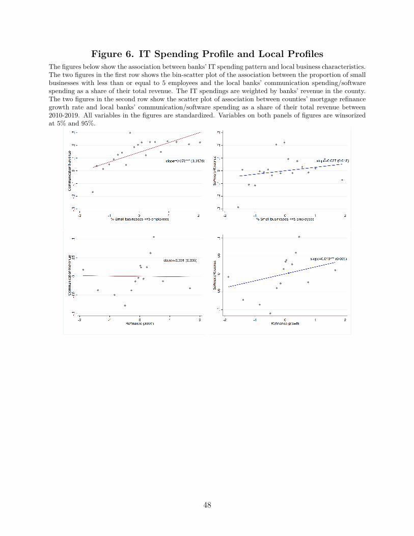
Figure 6. IT Spending Profile and Local ProfilesThe figures below show the association between banks’ IT spending pattern and local business characteristics.The two figures in the first row shows the bin-scatter plot of the association between the proportion of smallbusinesses with less than or equal to 5 employees and the local banks’ communication spending/softwarespending as a share of their total revenue. The IT spendings are weighted by banks’ revenue in the county.The two figures in the second row show the scatter plot of association between counties’ mortgage refinancegrowth rate and local banks’ communication/software spending as a share of their total revenue between2010-2019. All variables in the figures are standardized. Variables on both panels of figures are winsorizedat 5% and 95%.

48

Table 1. Sample CoverageThis table demonstrates the sample coverage of banks across five categories of banks’ size groups. All banksin the sample are commercial banks. The Call Report bank population includes only commercial banks(“Charter Type” being 200) following FFIEC definition. The first two columns shows the number of banksand the average asset sizes of banks in our sample, across five size groups. Column 3 and column 4 showthe total number of banks and average asset sizes of all banks in the Call Report. Column 5 shows thepercentage of sample coverage in terms of frequency compared with the population in Call Report, andcolumn 6 shows the percentage of sample coverage in terms of total asset size compared with the populationin Call Report.

Coverage of data Sample Call Report Freq % Asset %

Average Assets 2010-2019 (Billion) Num banks Ave Assets Num banks Ave Assets

>$250 Billion 6 1184.24 7 787.34 85.71% 96.66%$10 Billion–$250 Billion 88 42.30 106 43.69 83.02% 73.22%$1 Billion–$10 Billion 474 2.90 590 2.78 80.34% 89.43%$100 Million–$1 Billion 942 0.40 4161 0.32 22.64% 29.44%<$100 Million 296 0.06 2048 0.05 14.45% 14.23%

49

Table 2. IT Spending Summary StatisticsThis table shows the summary statistics of banks’ IT Spending. Total IT Spending is the sum of all typesof IT spending in millions of dollars. No. of IT employees is the total amount of IT-related employees.IT Spending/Revenue is total IT Spending scaled by banks’ total gross income, IT Spending/Non-interestexpense is total IT spending scaled by non-interest expenses; IT spending/Net income is total IT spendingscaled by total income minus the gross total expenses. The different categories of IT spending are the fourcategories of IT spending scaled by total IT spending.

Mean S.d. p(25) Median p(75)

Total IT Spending (Million) 7.311 111.354 0.030 0.215 1.056No. of IT Employees 133.434 872.102 7.000 21.578 56.400Storage Amount(PB) 3.517 25.522 0.107 0.476 1.779IT Spending/Revenue 0.031 0.155 0.003 0.010 0.023

IT Spending/Net income 0.597 18.475 0.018 0.051 0.135IT Spending/Expenses 0.037 0.191 0.004 0.012 0.028

IT Spending/Non-interest Expenses 0.044 0.213 0.005 0.014 0.034Communication/Total 0.092 0.117 0.028 0.052 0.105Software/Total 0.334 0.161 0.220 0.321 0.474Hardware/Total 0.171 0.119 0.063 0.158 0.235Services/Total 0.327 0.137 0.243 0.323 0.417Other/Total 0.056 0.099 0.008 0.014 0.062

50

Table 3. C&I Loans and Banks’ IT SpendingThis table presents the results of regression of banks’ C&I loan on the four major categories of banks’ ITspending and a vector of control variables at bank-year level. The sample period is 2010 to 2019.

Type S IT spendingRevenue i,10−19 = α+ β C&I Loan

Total loan i,10−19 + γX + εi

C&I Loan/Total Loan is commercial and industrial loan of bank i scaled by total loan between 2010-2019,Software/Rev is software spending scaled by total revenue, Communication/Rev is communication spendingscaled by total revenue, Hardware/Rev is Hardware spending scaled by total Revenue, Services/Rev. Controlvariables include net income scaled by total assets, deposits scaled by total assets, revenue per employee,salaries scaled by total assets and equity scaled by total assets. Both the left-hand side and the right-handside variables are taken the average across 2010-2019 within bank i. Fixed effects include Bank size, andbanks’ headquarter state fixed effects. ***, **, and * denote significance at the 1%, 5%, and 10% levels,respectively.

Software/Revenue Communication/Revenue Hardware/Revenue Services/Revenue

(1) (2) (3) (4)C& I loans/Total loan 0.031 0.050∗∗ 0.049∗∗ 0.043∗

(0.025) (0.024) (0.024) (0.025)Net income/Total Assets -0.142∗∗∗ -0.217∗∗∗ -0.242∗∗∗ -0.107∗∗∗

(0.028) (0.028) (0.028) (0.029)Deposits/Assets -0.013 0.028 0.032 -0.008

(0.031) (0.030) (0.030) (0.031)Revenue per Employee -0.267∗∗∗ -0.347∗∗∗ -0.301∗∗∗ -0.298∗∗∗

(0.035) (0.034) (0.034) (0.035)Salaries/Assets -0.018 -0.132∗∗∗ -0.099∗∗∗ -0.034

(0.026) (0.025) (0.025) (0.026)Equity/Assets 0.070∗∗ 0.051∗ 0.046∗ 0.071∗∗∗

(0.028) (0.027) (0.027) (0.028)Size FE Y Y Y YState FE Y Y Y YAdR-squared 0.098 0.162 0.150 0.110N 1798 1798 1798 1798

51

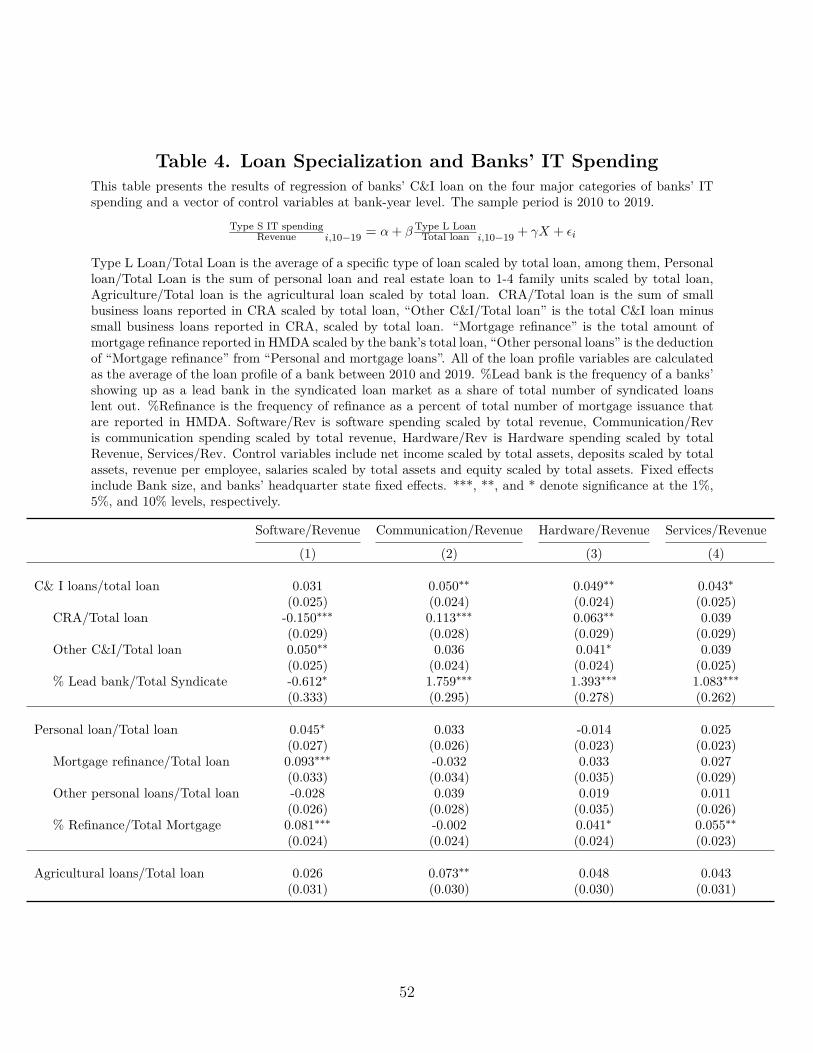
Table 4. Loan Specialization and Banks’ IT SpendingThis table presents the results of regression of banks’ C&I loan on the four major categories of banks’ ITspending and a vector of control variables at bank-year level. The sample period is 2010 to 2019.

Type S IT spendingRevenue i,10−19 = α+ βType L Loan

Total loan i,10−19 + γX + εi

Type L Loan/Total Loan is the average of a specific type of loan scaled by total loan, among them, Personalloan/Total Loan is the sum of personal loan and real estate loan to 1-4 family units scaled by total loan,Agriculture/Total loan is the agricultural loan scaled by total loan. CRA/Total loan is the sum of smallbusiness loans reported in CRA scaled by total loan, “Other C&I/Total loan” is the total C&I loan minussmall business loans reported in CRA, scaled by total loan. “Mortgage refinance” is the total amount ofmortgage refinance reported in HMDA scaled by the bank’s total loan, “Other personal loans” is the deductionof “Mortgage refinance” from “Personal and mortgage loans”. All of the loan profile variables are calculatedas the average of the loan profile of a bank between 2010 and 2019. %Lead bank is the frequency of a banks’showing up as a lead bank in the syndicated loan market as a share of total number of syndicated loanslent out. %Refinance is the frequency of refinance as a percent of total number of mortgage issuance thatare reported in HMDA. Software/Rev is software spending scaled by total revenue, Communication/Revis communication spending scaled by total revenue, Hardware/Rev is Hardware spending scaled by totalRevenue, Services/Rev. Control variables include net income scaled by total assets, deposits scaled by totalassets, revenue per employee, salaries scaled by total assets and equity scaled by total assets. Fixed effectsinclude Bank size, and banks’ headquarter state fixed effects. ***, **, and * denote significance at the 1%,5%, and 10% levels, respectively.

Software/Revenue Communication/Revenue Hardware/Revenue Services/Revenue

(1) (2) (3) (4)

C& I loans/total loan 0.031 0.050∗∗ 0.049∗∗ 0.043∗(0.025) (0.024) (0.024) (0.025)

CRA/Total loan -0.150∗∗∗ 0.113∗∗∗ 0.063∗∗ 0.039(0.029) (0.028) (0.029) (0.029)

Other C&I/Total loan 0.050∗∗ 0.036 0.041∗ 0.039(0.025) (0.024) (0.024) (0.025)

% Lead bank/Total Syndicate -0.612∗ 1.759∗∗∗ 1.393∗∗∗ 1.083∗∗∗(0.333) (0.295) (0.278) (0.262)

Personal loan/Total loan 0.045∗ 0.033 -0.014 0.025(0.027) (0.026) (0.023) (0.023)

Mortgage refinance/Total loan 0.093∗∗∗ -0.032 0.033 0.027(0.033) (0.034) (0.035) (0.029)

Other personal loans/Total loan -0.028 0.039 0.019 0.011(0.026) (0.028) (0.035) (0.026)

% Refinance/Total Mortgage 0.081∗∗∗ -0.002 0.041∗ 0.055∗∗(0.024) (0.024) (0.024) (0.023)

Agricultural loans/Total loan 0.026 0.073∗∗ 0.048 0.043(0.031) (0.030) (0.030) (0.031)

52

53

Table 5. Soft Information and Banks’ IT SpendingThis table presents the results of 2SLS and OLS discussed in Section 5.1. The first three columns show the results for the following specification:

∆ ln(CRA)i,c,post = µi + µ1 ln(1 + Qualified Small Buzs)c,pre + µ2Xi,c + εi,c

∆ ln(IT)i,c,post = αi + β ∆ ln(CRA)i,c,post + γXi,c + εi,c

The last two columns show the following OLS specification:

∆ ln(IT)i,c,post = αi + β × ∆ ln(CRA)i,c,post + µc + γXi,c + εi,c

∆ln (CRA)i,c,post is the change in average natural log of small business loans reported in CRA of bank i at county c in year during 2014-2017 comparedwith the 2010-2013, Software/Revenue is software spending scaled by total revenue, Communication/Revenue is communication spending scaled bytotal expenses, Hardware/Revenue is Hardware spending scaled by total expenses, Services/Revenue. The four IT spending scaled by revenue is atbank-county-year level. The control variable “Revenue per employee” is at bank-county level. County level control variables include the labor force,population growth rate, and total number of establishments. Fixed effects include bank fixed effects. ***, **, and * denote significance at the 1%, 5%,and 10% levels, respectively.

2SLS OLS

∆ CRA ∆ Software ∆ Communication ∆ Software ∆ Communication

(1) (2) (3) (4) (5)ln(Qualified Small Busi) 0.171∗∗∗

(0.023)∆ln(CRA) 0.018 0.070∗∗∗

(0.017) (0.017)∆ln(CRA) 0.003 0.014∗

(0.008) (0.008)Revenue per Employee 0.002 0.186∗∗∗ 0.188∗∗∗ 0.186∗∗∗ 0.189∗∗∗

(0.007) (0.008) (0.008) (0.008) (0.008)Bank FE Y Y Y Y YControls Y Y Y Y YF-statistics 20.23 53.43 98.66 53.31 97.07AdR-squared 0.431 0.157 0.147 0.157 0.146N 21202 21200 21195 21200 21195

54

Table 6. Hard Information and Banks’ IT SpendingThis table presents the results of regressions discussed in Section 5.2.The first three columns show the results for the 2SLS specification below:

ln(Refinance)i,c = µi + µ1Payments gapc + µ2Xi,c,t + εi,c,t

(Type S IT Spending

Revenue )i,c,t = αi + β ln(Refinance)i,c + γXi,c,t + εi,c,t

The last two columns show the results of OLS specification below:Type S IT spending

Revenue i,c,t = αi + µc + ln(Refinance)i,c,t + πt + β + γXi,c,t + εi,c,t

ln (Refinance)i,c,t is the amount of mortgage refinance loan issued by bank i in county c in year t. Payments gap is the hypothetical amount of interestpayments that could be saved due to the interest rate gap, if local households choose to refinance their mortgages during the year of 2011 and 2015.Software/Revenue is software spending scaled by total revenue, Communication/Revenue is communication spending scaled by total expenses. Controlvariables include net income scaled by total assets, deposits scaled by total assets, revenue per employee, salaries scaled by total assets and equity scaledby total assets, control variables are at bank-year level. Fixed effects include bank fixed effects, year fixed effects and county fixed effects. Standarderrors are clustered at county and bank level. ***, **, and * denote significance at the 1%, 5%, and 10% levels, respectively.

2SLS OLS

ln (Refinance) Software/Revenue Communication/Revenue Software/Revenue Communication/Revenue

(1) (2) (3) (4) (5)Payment gap 0.863∗∗∗

(0.037)ln(Refinance) 0.016∗∗∗ 0.007∗

(0.003) (0.003)ln(Refinance) 0.067∗∗ 0.037

(0.026) (0.025)Revenue per Employee -0.329∗∗∗ -0.334∗∗∗ -0.329∗∗∗ -0.332∗∗∗ -0.328∗∗

(0.004) (0.004) (0.004) (0.046) (0.078)Net income/Assets 0.009 0.002 0.009 -0.000 0.008

(0.009) (0.0092) (0.009) (0.021) (0.019)Equity/Assets -0.028∗∗ -0.014 -0.028∗∗ -0.014 -0.028

(0.011) (0.012) (0.012) (0.043) (0.022)Deposits/Assets 0.063∗∗∗ 0.153∗∗∗ 0.063∗∗∗ 0.141∗ 0.056

(0.016) (0.017) (0.016) (0.064) (0.034)Bank FE Y Y Y Y YYear FE Y Y Y Y YF Statistics 2408.16AdR-squared 0.018 0.008 0.018 0.438 0.450N 63189 63159 63189 63159 63189

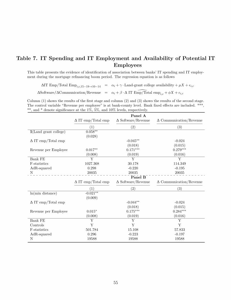
Table 7. IT Spending and IT Employment and Availability of Potential ITEmployees

This table presents the evidence of identification of association between banks’ IT spending and IT employ-ment during the mortgage refinancing boom period. The regression equation is as follows

∆IT Emp/Total Empi,c,15−19→10−14 = αi + γ · Land-grant college availability + µX + εi,c

∆Software/∆Communication/Revenue = αi + β · ∆ IT Emp/Total empi,c + φX + εi,c

Column (1) shows the results of the first stage and column (2) and (3) shows the results of the second stage.The control variable “Revenue per employee” is at bank-county level. Bank fixed effects are included. ***,**, and * denote significance at the 1%, 5%, and 10% levels, respectively.

Panel A∆ IT emp/Total emp ∆ Software/Revenue ∆ Communication/Revenue

(1) (2) (3)1(Land grant college) 0.058∗∗

(0.028)∆ IT emp/Total emp -0.045∗∗ -0.024

(0.018) (0.015)Revenue per Employee 0.017∗∗ 0.171∗∗∗ 0.279∗∗∗

(0.008) (0.019) (0.016)Bank FE Y Y YF-statistics 1027.368 30.178 114.349AdR-squared 0.298 -0.220 -0.195N 20035 20035 20035

Panel B∆ IT emp/Total emp ∆ Software/Revenue ∆ Communication/Revenue

(1) (2) (3)ln(min distance) -0.021∗∗

(0.009)∆ IT emp/Total emp -0.044∗∗ -0.024

(0.018) (0.015)Revenue per Employee 0.015∗ 0.175∗∗∗ 0.284∗∗∗

(0.008) (0.019) (0.016)Bank FE Y Y YControls Y Y YF-statistics 501.784 15.108 57.833AdR-squared 0.296 -0.223 -0.197N 19588 19588 19588

55

Appendix

Figure A1. Total Asset of Banks in SampleThis figure shows the sum of total asset size of all banks in our sample from 2010 to 2019 U.S. The reddashed line is the sum of call commercial banks’ asset size in U.S., data source is Board of Governors of theFederal Reserve System (US), Total Assets, All Commercial Banks [TLAACBW027SBOG]. The red solidline is the sum of total asset sizes of banks in our sample. The black solid line is the sample bank size outas a share of total nation-wide banks’ total asset size.

56

Figure A2. “Low Mortgage Rate Episode”This figure shows the time-series of aggregate mortgage interest rate and the Federal Funds Rates. ”MORT-GAGE30US” is the 30-Year Fixed Rate Mortgage Average in the United States from Freddie Mac. ”FED-FUNDS” is the effective Federal Funds Rate by Board of Governors of the Federal Reserve System.

57

Figure A3. McKinsey (2012) “Breakthrough IT Banking”

58

Figure A4. Definition of Different Types of IT Spending

(a) Figure A

(b) Figure B

(c) Figure C

(d) Figure D

59

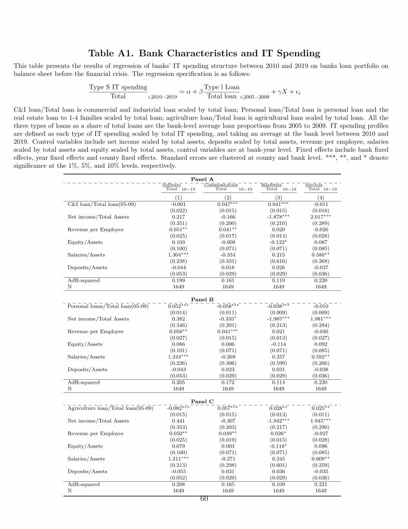
Table A1. Bank Characteristics and IT SpendingThis table presents the results of regression of banks’ IT spending structure between 2010 and 2019 on banks loan portfolio onbalance sheet before the financial crisis. The regression specification is as follows:

Type S IT spendingTotal i,2010−2019

= α+ βType l LoanTotal loan i,2005−2009

+ γX + εi

C&I loan/Total loan is commercial and industrial loan scaled by total loan; Personal loan/Total loan is personal loan and thereal estate loan to 1-4 families scaled by total loan; agriculture loan/Total loan is agricultural loan scaled by total loan. All thethree types of loans as a share of total loans are the bank-level average loan proportions from 2005 to 2009. IT spending profilesare defined as each type of IT spending scaled by total IT spending, and taking an average at the bank level between 2010 and2019. Control variables include net income scaled by total assets, deposits scaled by total assets, revenue per employee, salariesscaled by total assets and equity scaled by total assets, control variables are at bank-year level. Fixed effects include bank fixedeffects, year fixed effects and county fixed effects. Standard errors are clustered at county and bank level. ***, **, and * denotesignificance at the 1%, 5%, and 10% levels, respectively.

Panel ASoftware

Total 10−19Communication

Total 10−19Hardware

Total 10−19Services

Total 10−19

(1) (2) (3) (4)C&I loan/Total loan(05-09) -0.001 0.047∗∗∗ 0.041∗∗∗ -0.011

(0.022) (0.015) (0.015) (0.016)Net income/Total Assets 0.217 -0.166 -1.878∗∗∗ 2.017∗∗∗

(0.351) (0.200) (0.210) (0.289)Revenue per Employee 0.051∗∗ 0.041∗∗ 0.020 -0.026

(0.025) (0.017) (0.014) (0.028)Equity/Assets 0.103 -0.008 -0.122∗ 0.087

(0.100) (0.071) (0.071) (0.085)Salaries/Assets 1.304∗∗∗ -0.334 0.215 0.580∗∗

(0.238) (0.331) (0.616) (0.268)Deposits/Assets -0.044 0.018 0.026 -0.037

(0.053) (0.029) (0.029) (0.036)AdR-squared 0.199 0.161 0.110 0.220N 1649 1649 1649 1649

Panel BPersonal loans/Total loan(05-09) 0.052∗∗∗ -0.058∗∗∗ -0.038∗∗∗ -0.010

(0.014) (0.011) (0.009) (0.009)Net income/Total Assets 0.382 -0.335∗ -1.985∗∗∗ 1.981∗∗∗

(0.346) (0.201) (0.213) (0.294)Revenue per Employee 0.058∗∗ 0.041∗∗∗ 0.021 -0.030

(0.027) (0.015) (0.013) (0.027)Equity/Assets 0.086 0.006 -0.114 0.092

(0.101) (0.071) (0.071) (0.085)Salaries/Assets 1.244∗∗∗ -0.269 0.257 0.592∗∗

(0.226) (0.306) (0.599) (0.266)Deposits/Assets -0.043 0.023 0.031 -0.038

(0.053) (0.029) (0.029) (0.036)AdR-squared 0.205 0.172 0.114 0.220N 1649 1649 1649 1649

Panel CAgriculture loan/Total loan(05-09) -0.082∗∗∗ 0.057∗∗∗ 0.028∗∗ 0.025∗∗

(0.015) (0.015) (0.013) (0.011)Net income/Total Assets 0.441 -0.307 -1.942∗∗∗ 1.945∗∗∗

(0.353) (0.203) (0.217) (0.290)Revenue per Employee 0.050∗∗ 0.049∗∗ 0.026∗ -0.027

(0.025) (0.019) (0.015) (0.028)Equity/Assets 0.079 0.003 -0.118∗ 0.096

(0.100) (0.071) (0.071) (0.085)Salaries/Assets 1.211∗∗∗ -0.271 0.245 0.609∗∗

(0.213) (0.298) (0.601) (0.259)Deposits/Assets -0.055 0.031 0.036 -0.035

(0.052) (0.029) (0.029) (0.036)AdR-squared 0.208 0.165 0.109 0.221N 1649 1649 1649 1649

60

Table A2. Summary Statistics of Banks’ IT Spending by Bank Size GroupThis table presents the summary statistics of banks’ IT spending by banks’ size groups. Banks in the sampleare split into five groups. Total IT Spending is the sum of all types of IT spending in millions of dollars.No. of IT employees is the total amount of IT-related employees. IT Spending/Income is total IT Spendingscaled by banks’ total income, IT Spending/Non-interest expense is total IT spending scaled by non-interestexpenses; IT spending/Net income is total IT spending scaled by total income minus the gross total expenses.The different categories of IT spending are the four categories of IT spending scaled by total IT spending.

Mean S.d. Median< $100 MillionIT Spending/Revenue 0.015 0.048 0.005IT Spending/Expenses 0.019 0.075 0.007Communication/Total 0.159 0.176 0.086Software/Total 0.343 0.132 0.341Services/Total 0.330 0.138 0.340Hardware/Total 0.206 0.133 0.203

PC/Total 0.102 0.132 0.075Server/Total 0.100 0.127 0.066Terminal/Total 0.023 0.081 0.004Printer/Total 0.022 0.081 0.003Storage/Total 0.092 0.135 0.040

Other/Total 0.098 0.137 0.037

Mean S.d. Median$100 Million-$1 BillionIT Spending/Revenue 0.028 0.140 0.009IT Spending/Expenses 0.040 0.200 0.014Communication/Total 0.090 0.109 0.052Software/Total 0.370 0.155 0.348Services/Total 0.308 0.124 0.316Hardware/Total 0.167 0.115 0.158

PC/Total 0.066 0.090 0.053Server/Total 0.070 0.087 0.052Terminal/Total 0.012 0.047 0.004Printer/Total 0.011 0.047 0.003Storage/Total 0.051 0.091 0.022

Other/Total 0.056 0.097 0.014

Mean S.d. Median$1 Billion-$10 BillionIT Spending/Revenue 0.043 0.193 0.014IT Spending/Expenses 0.062 0.262 0.021Communication/Total 0.064 0.078 0.042Software/Total 0.272 0.166 0.231Services/Total 0.361 0.152 0.336Hardware/Total 0.165 0.117 0.140

PC/Total 0.056 0.064 0.043Server/Total 0.065 0.063 0.050Terminal/Total 0.007 0.021 0.004Printer/Total 0.007 0.022 0.003Storage/Total 0.033 0.061 0.017

Other/Total 0.036 0.072 0.012

Mean S.d. Median$10 Billion-$250 BillionIT Spending/Revenue 0.045 0.249 0.012IT Spending/Expenses 0.067 0.310 0.019Communication/Total 0.055 0.052 0.042Software/Total 0.283 0.161 0.233Hardware/Total 0.147 0.105 0.108Services/Total 0.335 0.137 0.293

PC/Total 0.047 0.041 0.029Server/Total 0.057 0.041 0.038Terminal/Total 0.006 0.009 0.004Printer/Total 0.005 0.010 0.003Storage/Total 0.027 0.036 0.011

Other/Total 0.032 0.057 0.010

Mean S.d. Median> $250 BillionIT Spending/Revenue 0.019 0.049 0.005IT Spending/Expenses 0.031 0.075 0.008Communication/Total 0.046 0.041 0.031Software/Total 0.268 0.137 0.228Services/Total 0.357 0.149 0.328Hardware/Total 0.158 0.103 0.138

PC/Total 0.051 0.043 0.039Server/Total 0.062 0.044 0.050Terminal/Total 0.007 0.011 0.004Printer/Total 0.006 0.012 0.003Storage/Total 0.031 0.039 0.018

Other/Total 0.036 0.061 0.012

61

Table A3. Bank Size, Loan Information Nature and Banks’ IT SpendingThis table presents the results of regression of Banks’ IT spending response when small business loans andmortgage refinance volume increases, interacting with bank size. This table focuses on software spending andcommunication spending. The left-hand side variables are software spending as a share of total revenue andcommunication spending as a share of total revenue respectively. The right-hand side variables are banks’small business loans and mortgage refinance respectively, interacting with banks’ size groups. ”Small” isdefined as banks with average asset size less than $100 million between 2010-2019, ”Medium” is defined asbanks with average asset size $100 million-$10 billion between 2010-2019, ”Large” is defined as banks withaverage asset size greater than 10 $ Billion between 2010-2019. Control variables include net income scaledby total assets,deposits scaled by total assets, revenue per employee, salaries scaled by total assets and equityscaled by total assets, control variables are at bank-year level. Fixed effects include bank fixed effects, yearfixed effects and county fixed effects. Standard errors are clustered at county and bank level. ***, **, and* denote significance at the 1%, 5%, and 10% levels, respectively.

Software/Revenue Communication/Revenue

(1) (2) (3) (4)(Small) × ln(CRA) -0.015 0.023

(0.045) (0.046)(Medium) × ln(CRA) -0.008 0.029∗∗∗

(0.007) (0.006)(Large) × ln(CRA) 0.015 0.031∗∗∗

(0.012) (0.011)(Small) × ln(Mortgage refinance) -0.002 -0.006

(0.006) (0.006)(Medium) × ln(Mortgage refinance) 0.016∗∗ 0.007

(0.006) (0.006)(Large) × ln(Mortgage refinance) 0.034∗∗∗ -0.046∗∗∗

(0.010) (0.010)Fixed effects Bank, County, YearBank Controls Y Y Y YAdR-squared 0.533 0.525 0.540 0.532N 160214 156718 160259 156762

62

Table A4. Small Business Loan, Mortgage Refinance and Bank IT Spending: IIThis table presents regression results of banks’ new mortgage issuance on the four major categories of banks’IT spending and relevant control variables at bank-county-year level. The sample period is 2010 to 2019.

Type S IT spendingRevenue i,c,t = αi + µc,t + βln(refinance)i,c,t or ln(CRA)i,c,t + γX + εi,c,t

ln refinancei,c,t is the natural logarithm of newly mortgage refinance of bank i at county c in year t in reportedin HMDA, ln CRAi,c,t is the natural logarith of small business loans issued by bank i in county c and inyear t. Software(Communication)/Revenue is software (communication) spending scaled by total revenue,measured at bank-county-year level. Control variables include net income scaled by total assets, depositsscaled by total assets, revenue per employee, salaries scaled by total assets and equity scaled by total assets,control variables are at bank-year level. Fixed effects include bank fixed effects, county × year. Standarderrors are clustered at county and bank level. ***, **, and * denote significance at the 1%, 5%, and 10%levels, respectively.

Panel ASoftware/Revenue Communication/Revenue

(1) (2) (3) (4) (5) (6)ln(refinance) 0.027∗∗∗ 0.035∗∗∗ 0.034∗∗∗ -0.002 0.003 0.002

(0.006) (0.007) (0.010) (0.008) (0.007) (0.007)Revenue per Employee -0.213∗∗∗ -0.225∗∗∗ -0.228∗∗∗ -0.236∗∗∗

(0.014) (0.015) (0.011) (0.012)Net income/Assets 0.004 0.004 0.028∗∗∗ 0.033∗∗

(0.011) (0.012) (0.010) (0.014)Equity/Assets 0.013 0.003 -0.007 -0.012

(0.028) (0.027) (0.011) (0.012)Deposits/Assets 0.104 0.106∗ 0.022 0.024

(0.070) (0.060) (0.029) (0.023)Salaries/Assets -1.560 -1.382 -0.899 -0.800

(1.064) (1.089) (1.281) (1.349)Fixed effects Bank, County×YearBank Controls Y Y Y Y Y YAdR-squared 0.449 0.477 0.487 0.468 0.496 0.501N 179713 176486 159732 179759 176532 159778

Panel BSoftware/Revenue Communication/Revenue

(1) (2) (3) (4) (5) (6)ln(CRA) 0.005 0.006∗ 0.006 0.014∗∗∗ 0.014∗∗∗ 0.014∗∗∗

(0.004) (0.004) (0.004) (0.003) (0.003) (0.003)Revenue per Employee -0.212∗∗∗ -0.224∗∗∗ -0.228∗∗∗ -0.235∗∗∗

(0.014) (0.015) (0.011) (0.012)Net income/Assets 0.003 0.002 0.026∗∗ 0.028∗∗

(0.010) (0.011) (0.010) (0.013)Equity/Assets 0.011 0.002 -0.006 -0.010

(0.028) (0.027) (0.011) (0.012)Deposits/Assets 0.097 0.101∗ 0.022 0.025

(0.068) (0.059) (0.029) (0.023)Salaries/Assets -0.702 -0.548 -0.394 -0.304

(0.825) (0.880) (0.988) (1.049)Fixed effects Bank, County×YearBank Controls Y Y Y Y Y YAdR-squared 0.459 0.485 0.497 0.479 0.506 0.511N 184314 181056 163775 184363 181105 163824

63

Table A5. IT Spending and IT EmploymentThis table presents the results of association between banks’ IT investment and banks’ employment, with adistinction between IT employees and non-IT employees. The regression equations are as follows:

∆ ln IT Emp or ∆ ln Non-IT employees =β∆ln(Software spending)i,c,t or ∆ln(Communication spending)i,c,t

+ αi,t + µc,t + γX + εi,c,t

∆log IT Emp and ∆log Non-IT Emp are the logarithm of IT related employees and Non-IT related employeesrespectively. Software/Revenue is software spending scaled by total revenue, Communication/Revenue iscommunication spending scaled by total revenue. The IT spending scaled by revenue is at bank-county-yearlevel. Control variables include net income scaled by total assets, deposits scaled by total assets, revenue peremployee, salaries scaled by total assets and equity scaled by total assets, control variables are at bank-yearlevel. Fixed effects include bank-year fixed effects and county-year fixed effects. Standard errors are clusteredat county and bank level. ***, **, and * denote significance at the 1%, 5%, and 10% levels, respectively.

∆ ln IT Emp ∆ ln Non-IT Emp ∆ ln IT Emp ∆ ln Non-IT Emp

(1) (2) (3) (4)∆ ln Software -0.148∗∗∗ -0.117∗∗∗

(0.051) (0.043)∆ ln Communication 0.043∗∗ 0.086∗∗∗

(0.022) (0.022)County×Year FE Y Y Y YBank×Year FE Y Y Y YControl Y Y Y YAdR-squared 0.237 0.231 0.236 0.232N 148617 148617 148617 148617

64