In cooperation with the National Aeronautics and Space Administration Ames Research Center

Investigations into Near-real-time Surveying for Geophysical Data Collection using an Autonomous Ground Vehicle

Open File Report 2014–1013

U.S. Department of the Interior U.S. Geological Survey

COVER: Figure showing magnetic data downloaded from an unmanned vehicle after an exploratory survey in Field Park, California. Background satellite imagery from Google Maps. Figure by G. Phelps.

In cooperation with the National Aeronautics and Space Administration Ames Research Center

Investigations into Near-real-time Surveying for Geophysical Data Collection using an Autonomous Ground Vehicle

By G. Phelps, C. Ippolito, R. Lee, J. Spritzer, and Y. Yeh

Open File Report 2014–1013

U.S. Department of the Interior U.S. Geological Survey

U.S. Department of the Interior SALLY JEWELL, Secretary

U.S. Geological Survey Suzette M. Kimball, Acting Director

U.S. Geological Survey, Reston, Virginia: 2014

For more information on the USGS—the Federal source for science about the Earth, its natural and living resources, natural hazards, and the environment—visit http://www.usgs.gov or call 1-888-ASK-USGS

For an overview of USGS information products, including maps, imagery, and publications, visit http://www.usgs.gov/pubprod

To order this and other USGS information products, visit http://store.usgs.gov

Suggested citation: Phelps, G., Ippolito, C., Lee, R., Spritzer, J., and Yeh, Y., 2014, Investigations into near-real-time surveying for geophysical data collection using an autonomous ground vehicle: U.S. Geological Survey Open-File Report 2014–1013, 18 p., http://dx.doi.org/10.3133/ofr20141013.

ISSN 2331-1258 (online)

Any use of trade, product, or firm names is for descriptive purposes only and does not imply endorsement by the U.S. Government.

Although this report is in the public domain, permission must be secured from the individual copyright owners to reproduce any copyrighted material contained within this report.

iii

Contents Abstract .......................................................................................................................................................................... 1 Introduction .................................................................................................................................................................... 1 The Autonomous Ground Vehicle .................................................................................................................................. 2 The Flood Park Experiment ............................................................................................................................................ 3 Data Processing ............................................................................................................................................................. 6 Discussion .................................................................................................................................................................... 11 Conclusions.................................................................................................................................................................. 11 References Cited ......................................................................................................................................................... 12

Figures Figure 1. Photographs showing the autonomous ground vehicle (MAX 5) developed by researchers at Carnegie Mellon Innovations Laboratory and National Aeronautics and Space Administration. A, MAX 5 rover; B, MAX 5 rover with mounted magnetometers. ...........................................................................................................................3 Figure 2. Aerial photo of the Flood Park, California, study area showing a grid of the ground magnetic data and survey traverse lines. Purple lines indicate exploratory survey traverse; red lines indicate targeted survey traverse. Background satellite imagery from Microsoft Bing, served through ArcMap. ..............................................................4 Figure 3. Flood Park, California, exploratory survey, midway through the survey, showing magnetic data downloaded from the rover, interpolated on-the-fly, and displayed on-screen at the base station. Warm colors represent regions of high magnetism, and cool colors represent regions of low magnetism. Background satellite imagery from Google Maps. ........................................................................................................................................5 Figure 4. Sample data window showing raw data and data with diurnal magnetic variation removed, Flood Park, California, survey area. ...............................................................................................................................................8 Figure 5. Final interpolated magnetic field for A, the exploratory and B, the targeted surveys, Flood Park, California. Background satellite imagery from Microsoft Bing, served through ArcMap. ........................................... 10

iv

Conversion Factors Inch/Pound to SI

Multiply By To obtain

Length inch (in.) 2.54 centimeter (cm)

inch (in.) 25.4 millimeter (mm)

foot (ft) 0.3048 meter (m)

yard (yd) 0.9144 meter (m)

Velocity foot per second (ft/s) 0.3048 meter per second (m/s)

mile per hour (mi/h) 1.609 kilometer per hour (km/h)

Mass ounce, avoirdupois (oz) 28.35 gram (g)

pound, avoirdupois (lb) 0.4536 kilogram (kg)

Density pound per cubic foot (lb/ft3) 16.02 kilogram per cubic meter

(kg/m3)

pound per cubic foot (lb/ft3) 0.01602 gram per cubic centimeter (g/cm3)

SI to Inch/Pound

Multiply By To obtain

Length centimeter (cm) 0.3937 inch (in.)

millimeter (mm) 0.03937 inch (in.)

meter (m) 3.281 foot (ft)

meter (m) 1.094 yard (yd)

Velocity meter per second (m/s) 3.281 foot per second (ft/s)

kilometer per hour (km/h) 0.6214 mile per hour (mi/h)

Mass gram (g) 0.03527 ounce, avoirdupois (oz)

kilogram (kg) 2.205 pound avoirdupois (lb)

Density kilogram per cubic meter (kg/m3) 0.06242 pound per cubic foot (lb/ft3)

gram per cubic centimeter (g/cm3) 62.4220 pound per cubic foot (lb/ft3)

1

Investigations into Near-real-time Surveying for Geophysical Data Collection using an Autonomous Ground Vehicle

By G. Phelps, 1 C. Ippolito, 2 R. Lee, 2, J. Spritzer, 1 and Y. Yeh 2

Abstract The U.S. Geological Survey and the National Aeronautics and Space Administration are

cooperatively investigating the utility of unmanned vehicles for near-real-time autonomous surveys of geophysical data collection. Initially focused on unmanned ground vehicle collection of magnetic data, this cooperative effort has brought unmanned surveying, precision guidance, near-real-time communication, on-the-fly data processing, and near-real-time data interpretation into the realm of ground geophysical surveying, all of which offer advantages over current methods of manned collection of ground magnetic data. An unmanned ground vehicle mission has demonstrated that these vehicles can successfully complete missions to collect geophysical data, and add advantages in data collection, processing, and interpretation. We view the current experiment as an initial phase in further unmanned vehicle data-collection missions, including aerial surveying.

Introduction The U.S. Geological Survey (USGS) and the National Aeronautics and Space Administration

(NASA) are engaging in a collaborative effort to develop and test near-real-time surveying methods using autonomous unmanned vehicles whereby data are collected, processed, analyzed, and interpreted during the mission. The autonomous unmanned vehicles are engineered to accomplish intelligent guidance, navigation, and control for the vehicle to meet mission objectives.

Historically, technological limitations required geophysical data collection and analysis to be performed separately. Until recently, data collection had to be performed manually by moving and operating instruments to collect data either on foot, or with the instrument towed behind a manned-vehicle. This task is generally tedious and often labor-intensive, and only rudimentary tools have been available to assess data quality. As a result, data are processed in the office, where computers are typically powerful enough to perform data reduction, analysis and interpretation. Additional data required for follow-on investigations are typically performed during the next field session.

The advent of modern technology now allows for most geophysical processing and analysis to be performed in the field in near-real-time. One significant advantage is that data quality can be assessed at the time the data are being collected. Another advantage is that the survey can be modified as it progresses to better meet the scientific goals. An investigator would be able to choose, for example, whether to spend the remaining field time investigating a newly discovered target in greater detail, or to expand the survey and look for new targets. A third advantage is that on-the-fly processing paves the way for payload-directed missions—missions where the autonomous vehicle itself analyzes the incoming data and makes rudimentary decisions on how to proceed based on a set of programmed criteria.

Unmanned vehicles offer several significant advantages over manned surveying. Unmanned precision guidance allows for exact and repeatable data collection. Additionally, unmanned vehicles can perform “dirty and dangerous” missions, performing maneuvers or flying over areas where risk to

2

human life is high. For example, unmanned aerial vehicles have the ability to fly 35 m off the ground, an altitude typically off limits to manned aircraft. Flying close to the ground significantly increases data resolution for a number of sensors, including magnetometers. Near-real-time communication can deliver incoming data locally to a base station for review, processing, and analysis by the investigating scientists. Communication over the Internet significantly expands the pool of participants; a team of engineers and scientists at different locations can have simultaneous access and input to the survey using a Web site. On-the-fly data processing delivers interpretable scientific data in near real time. Furthermore, intelligent systems can perform rudimentary analytical tasks, such as data contouring, or a continually updated gradient analysis of a potential field as it is being measured. The investigating scientists can then analyze the geophysical data and generate preliminary interpretations during deployment. Consequently, the investigating scientists can modify the current survey or implement follow-on investigations based on the incoming data and their ongoing interpretations. Unmanned surveying even holds the promise of automated intelligent data processing by the unmanned vehicles themselves, which could be programmed to modify the data-collection mission in specific ways, according to pre-programmed conditions of interest. For example, processing onboard an unmanned vehicle could be programmed to identify targets that generate a circular pattern in the contoured data and to re- survey these targets at a higher resolution.

Advances in robotics and automation have lead to autonomous vehicles; that is, vehicles that drive themselves. In this paper we make a distinction between unmanned ground and aerial vehicles (UGVs and UAVs, respectively) and autonomous ground and aerial vehicles (AGVs and AAVs, respectively). UGVs and UAVs are vehicles that are always under manned control, remotely piloted from a ground station. AGVs and AAVs are fully autonomous, using intelligent algorithms to guide the vehicle. Although for safety reasons a pilot is always present during missions and able to take direct control of the vehicle, under normal operating conditions the pilot is simply an observer. The vehicle is programmed to follow a pre-determined survey path. The vehicle executes the survey, collecting data and relaying it back to the base station.

In this experiment we apply autonomous vehicles in geophysical surveying that enable near-real-time data processing, analysis, and interpretation. The goal was to investigate the workflow of autonomous near-real-time surveys using AGVs to collect data along precisely located, repeatable paths, to process and display the data as soon as possible to allow time for interpretation and, potentially, survey modification.

The Autonomous Ground Vehicle The MAX 5 is an unmanned rover designed at Carnegie Mellon Innovations Laboratory in a

collaborative effort between Carnegie Mellon University and NASA. The MAX 5 rover (fig. 1) is a small off-the-shelf remote-controlled vehicle modified to have autonomous navigation. It is battery-powered, has a maximum speed of approximately 5 m/s, and a payload of up to 10 kg. Its dimensions are approximately 46 by 38 by 48 cm. The rover is outfitted with a NovAtel OEM-G4-G2 DGPS for precision navigation, and it can be configured to transmit and receive data and navigational controls from the base station using either a 900-MHz spread spectrum radio modem or a standard IEEE 802.11g wireless protocol. An onboard Intel Centrino 1.6-GHz Pentium-M CPU computer directs the rover and manages incoming and outgoing data (Lee and others, 2010).

3

Figure 1. Photographs showing the autonomous ground vehicle (MAX 5) developed by researchers at Carnegie Mellon Innovations Laboratory and National Aeronautics and Space Administration. A, MAX 5 rover; B, MAX 5 rover with mounted magnetometers.

The rover’s small size limits the terrain it can negotiate; flat, firm ground, such as manmade surfaces like pavement or lawns, or naturally flat surfaces like playas, offer the best places to survey.

We mounted two Geometrics model 858® cesium vapor magnetometers on the MAX 5 rover (fig. 2). The magnetometers were mounted on an aluminum pole 1 m from the body of the rover to minimize magnetic noise generated from the rover engine and electrical system. In addition, the engine was wrapped in mu-metal, a magnetic-shielding metal, to further minimize platform noise. The console for the magnetometers was towed behind the MAX 5 and connected to the main telemetry system by an RS232 serial connection.

The base station is an ordinary pentium quad-core laptop, with 4 GB of RAM, running the Windows 7 operating system. Reflection, proprietary software developed by NASA and written in C++, performs multiple mission-critical functions, and it is the base station used for the DGPS real-time location correction. It provides two-way communication with the rover using the 900-MHz radio link, enabling the sending of remote commands and the ability for manual joystick override control. Finally, the base station manages data download, and real-time display of both raw and processed data and maps through simulated airplane cockpit displays.

The Flood Park Experiment We conducted an experiment at Flood Park, Menlo Park, Calif. (fig. 3). The Hetch Hetchy

Aqueduct passes beneath the baseball field in the park and offered an ideal setting to test the rover’s performance. The aqueduct is a subsurface manmade conduit with high iron content, which we expected would generate a significant magnetic anomaly resulting from a large magnetization induced by the Earth’s local magnetic field.

4

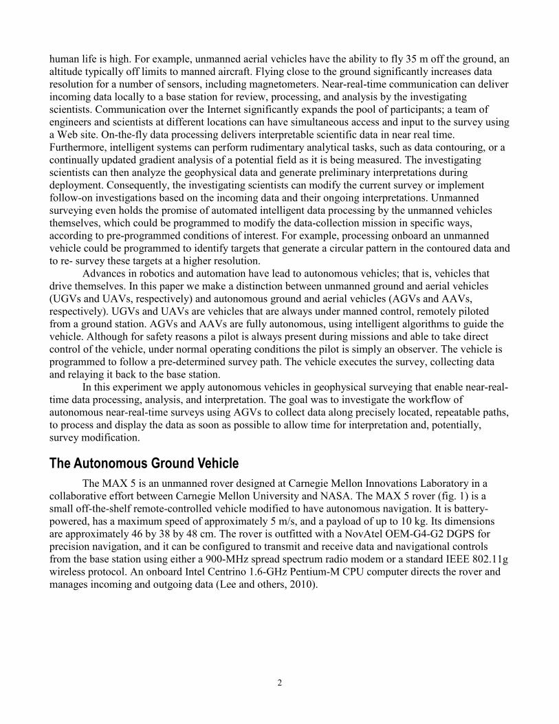
Figure 2. Aerial photo of the Flood Park, California, study area showing a grid of the ground magnetic data and survey traverse lines. Purple lines indicate exploratory survey traverse; red lines indicate targeted survey traverse. Background satellite imagery from Microsoft Bing, served through ArcMap.

5

Figure 3. Flood Park, California, exploratory survey, midway through the survey, showing magnetic data downloaded from the rover, interpolated on-the-fly, and displayed on-screen at the base station. Warm colors represent regions of high magnetism, and cool colors represent regions of low magnetism. Background satellite imagery from Google Maps.

6

To simulate a survey where the target was not known, we constructed an initial exploratory survey path that covered most of the baseball field (fig. 3). The survey design was to drive the rover along a grid pattern of lines over an 80 by 60 ft. rectangle at approximately 5-ft. spacing, with primary lines trending northeast and crossing (tie) lines trending northwest. The goals of the survey were (1) to test the viability of using an AGV to collect and process data on-the-fly with accuracy sufficient to allow preliminary scientific interpretation in near-real-time, and (2) to test the system’s ability to perform a targeted study of specific anomalies identified in the initial, exploratory survey.

Setup of the rover and base station took approximately 1 hour. Coordinates were input at the base station by choosing the corner coordinates of a rectangular survey pattern and the line spacing, and by calculating a row-prime order pattern to traverse the survey area. The data were relayed back to the base station each time the MAX 5 reached the easternmost end of a line. The MAX 5 took approximately 30 minutes to complete the exploratory survey and less than 25 minutes to complete the targeted survey.

During the survey, magnetic data and location information received from the rover by the base station were interpolated using the bicubic spline algorithm of Briggs (1974). A color map of the magnitude of the measured magnetic field was generated and displayed on Google EarthTM images. The map was updated every 3 seconds as new data were acquired. As the survey progressed, a significant magnetic anomaly began to take shape; being able to see the anomaly displayed just after it was detected allowed for the planning and execution of a second survey. The exploratory survey showed an east-trending, linear magnetic body whose magnetic anomaly was significantly higher than the regional magnetic field. By the end of the exploratory survey, we had a plan for a targeted survey. Taking advantage of the exploratory data, we designed the follow-on targeted survey lines to be collected perpendicular to the observed linear structure. Within minutes the coordinates for the targeted survey were input, and the MAX 5 was re-deployed, collecting data for a second, more detailed map of the measured magnetic field directly over the area of interest. Figure 3 shows an image screen capture taken near the end of the second survey.

Total field time was roughly 3 hours, including setup and breakdown. Total surveying time was approximately 1 hour.

Data Processing Processing data from magnetic surveys involves several steps: removing dropouts from the

instrument data stream; correction for magnetic noise caused by both the induced and remanent magnetization of the platform (for example, remanent magnetization from iron-bearing vehicle parts, and induced magnetization from vehicle parts, electrical equipment, and eddy currents in the vehicle frame); correction for diurnal effects; survey leveling; removal of the International Geomagnetic Reference Field, the long-wavelength magnetic field of the Earth (which, over this small survey area, is essentially constant); and removal of any regional trend. Each of these effects was assessed either during the survey or in post-processing of the data. The limited scope of the project did not enable the researchers to investigate compensation for all of these effects, although doing so would be a natural next step for future experiments.

Dropouts, which occur when the data stream is momentarily interrupted by electromagnetic interference, were coded as zeros and thus easily filtered from the data stream at the base station.

Platform noise was minimized by attaching the magnetometer sensors onto an aluminum pole that extended two feet from the MAX 5, encasing the engine in mu-metal, and creating a small, flat, mu-metal shield perpendicular to the pole and placed close to the MAX 5. Controlled stationary testing revealed that that the MAX 5’s engine and navigational gears contributed an insignificant level of noise (several nT) compared with the magnitude of the targeted anomaly (with an amplitude of approximately 8,000 nT). We assumed that the effect of heading error due to the magnetic field of the MAX 5 and the

7

magnetic field caused by the motion of the platform was negligible. The effect of the heading error can be seen best at the edges of the prominent horizontal magnetic anomaly in fig. 5B, where the anomaly is shifted in an alternating north-south pattern by approximately 5 ft. The effect is visible, but minor compared to the magnitude of the magnetic anomaly.

Diurnal magnetic corrections were subtracted from the data subsequent to the survey by using daily magnetic variations recorded at Jasper Ridge, an instrumented station near Stanford University (approximately 5 miles from the survey area), managed jointly by Stanford and Geometrics, Inc. The station logs the 0.1-Hz signal of the daily variations of the total magnetic field, and the files are accessible on the Internet to cooperating agencies. The data are time-stamped at 0.1-second intervals, a finer interval than the 0.2-second intervals, during which roving data were collected. A single 0.2-second value was interpolated from the diurnal data to match the time stamp of the survey magnetic data, and the diurnal variation was normalized by subtracting the mean of the diurnal data from the diurnal data. The normalized diurnal variation was then subtracted from the survey data to correct for the diurnal effect. The magnitude of the diurnal variation was less than 1 percent of the magnitude of the total observed magnetic variation. Because the diurnal correction does not substantially affect the magnetic signal of the subsurface target (fig. 4), it was not performed during the survey. Incorporating the diurnal correction into the near-real-time workflow would require setting up an additional magnetometer near the base station, specifically for collecting near-real-time diurnal magnetic data. These data could be streamed to the base station and subtracted from the survey data as it is collected. Doing so would be necessary during times of exceptionally large diurnal change, where the target anoamaly is small, or during prolonged missions.

8

Figure 4. Sample data window showing raw data and data with diurnal magnetic variation removed, Flood Park, California, survey area.

Survey leveling is the process by which repeat measurements across a survey are reconciled (Luyendik, 1997). Typically, data is collected along a series of parallel lines, which represent the bulk of the data collection for a survey. A few lines of data (called “tie lines”) are collected perpendicular to the initial parallel lines and are used to correct for the temporal variation of the survey data. The tie lines provide repeat measurements where they cross the initial parallel lines. The process of leveling has historical importance because many aeromagnetic surveys were not diurnally corrected (see, for example, Yarger and others, 1978). Additionally, many surveys were flown prior to the invention of GPS surveying, so location of the data was approximate. Leveling is important for distributing the errors caused by the diurnal effect and imprecisely located data, two effects that are significantly reduced by directly accounting for the diurnal effect and DGPS locations. Thus, for the surveys described in this paper, leveling distributes data-collection errors, such as those that may be caused by significant rotation of the platform during the survey, or by platform noise.

The Flood Park survey was originally designed to have multiple tie lines. However, about halfway through the tie-line survey, the platform experienced mechanical problems. Because the rover

9

was at maximum capacity for load weight, the motor was prone to overheating. This became a significant problem during the tie-line survey, at which point the decision was made to abandon the tie-line survey and attempt to complete the detailed survey. Because the target had been identified, the tie-line survey was abandoned in favor of the targeted survey, which did not include tie lines owing to time constraints. For this experiment, leveling the data had little effect on the outcome because the signal of the target was large compared to any noise introduced. However, incorporating survey leveling is important for surveys with a lower signal-to-noise ratio and, like the diurnal correction, could be incorporated directly into the near-real-time data processing, updating adjustments to the incoming data as new tie-line information is collected when survey lines cross.

The International Geomagnetic Reference Field (IGRF) was calculated using Phillips’ (2007) toolset and removed from the data subsequent to the survey. The residual magnetic field was then interpolated to a regular grid using a completely regularized spline (Mitasova and Mitas, 1993), with an isotropic search radius for the exploratory survey (fig. 5A). Once the linear structure of the magnetic body was revealed with the exploratory survey, the spatial structure of the magnetic field could be observed. This structure is linear and trending east, and data are correlated east-west to a higher degree than north-south. An anisotropic search radius was, therefore, used to interpolate the targeted survey, with a higher correlation length used for the east-west direction. This results in an interpolated anomaly that is more continuous along its length than its width (fig. 5B).

10

Figure 5. Final interpolated magnetic field for A, the exploratory and B, the targeted surveys, Flood Park, California. Background satellite imagery from Microsoft Bing, served through ArcMap.

11

Discussion The success of this survey was dependent upon the large signal-to-noise ratio of the target to

diurnal variations or magnetic noise from the platform. Some steps in the data processing (diurnal correction, removal of the IGRF) were accomplished after the survey was completed, and some of the data processing steps (heading correction, survey leveling) were not done. In this particular case, the exclusion of these processing steps does not significantly alter the results (compare fig. 3 to fig. 5). However, such processing should be incorporated into the workflow for future surveys in order to maximize the effectiveness of the near-real-time workflow.

The MAX 5 rover was sufficient for completing the experimental survey, but is not robust enough for most geologic surveys, which require surveying over rough terrain. Even during this survey, the MAX 5 experienced setbacks. The sensor mount (aluminum pole) was somewhat unstable. The sensors added weight to the end of the pole, and as the platform moved over small grass hummocks the sensor underwent vertical displacements of approximately ±0.1 m with respect to the platform. In addition, changes in the dip angle of the front of the rover translated into larger changes in vertical movement at the end of the pole where the sensors were attached. The overall effect was that the average vertical position of the sensor (with respect to the ground) varied locally by ±10 cm. This motion could introduce significant measurement inconsistencies for any target located at or near the surface, because the sensor distance can change by a factor of 2. The effect for this experiment was negligible, however, owing to the size and distance of the target from the land surface.

Another limitation resulted from the MAX 5 being loaded to its weight limit. As a result, the system was prone to overheating during the experiment, requiring the survey to be paused twice during the mission to allow the MAX 5 motors time to cool.

Despite setbacks, the Flood Park survey had several successes: two unmanned surveys, near-real-time data collection and processing, and near-real-time data interpretation that allowed for the design and implementation of a second, targeted survey. The setbacks led to suggestions for improving autonomous adaptive surveying for the collection of magnetic data. These improvements can be separated into tasks for the platform, sensor processing, and near-real-time analysis.

Improvements to the platform could include using a platform with greater physical abilities, allowing for heavier payload capability, greater power supply, and more versatility in rough terrain, and developing an aerial platform as an alternative to ground platforms.

Improvements to the sensor processing could include better characterizing and compensating for the magnetic field of the platform produced by its frame, engines, and electronics.

Improvements in near-real-time analysis could include integrating the diurnal correction and survey leveling into the near-real-time data processing, including gradient analysis during the field-interpretation phase, and including intelligent algorithms that match incoming data to mathematical models of targets, highlighting these data for the users, and executing new, detailed survey paths over the highlighted regions.

Conclusions We have demonstrated that a near-real-time surveying approach for collecting, processing, and

interpreting geophysical magnetic data, using autonomous ground vehicles, is now possible. Such a near-real-time approach offers potential advantages over standard, manned ground magnetic data collection. For geophysical data collection, a survey can be modified and tailored to address problems of interest as they arise, increasing the efficiency of surveying. Current limitations to near-real-time missions are due to platform limitations, such as payload capacity, supplied power, and terrain roughness. The MAX 5 magnetic data experiment illustrates the capabilities and potential of autonomous geophysical surveying and paves the way for future improvements in the approach.

12

Currently, the disadvantages to surveying with an AGV or AAV include the need for a specialized crew (in addition to the personnel needed for data collection) to run and troubleshoot the unmanned vehicles, the need for onsite power, and the potential limitations of the type of vehicle available for data collection.

References Cited Briggs, I., 1974, Machine contouring using minimum curvature: Geophysics, v. 39, no. 1, p. 39–48. Lee, R., Yeh, Y., and Ippolito, C., 2010, Payload-directed control of geophysical magnetic surveys: 51st

AIAA/ASME/ASCE/AHS/ASC Structures, Structural Dynamics, and Materials Conference, Orlando, Fla., April 12–15.

Luyendyk, A.P.J., 1997, Processing of airborne magnetic data: Journal of Australian Geology and Geophysics, v. 17, no. 2, p. 31–38.

Mitasova, H., and Mitas, L., 1993, Interpolation by regularized spline with tension: I—Theory and implementation: Mathematical Geology, v. 25, no. 6, p. 641–655.

Phillips, J.D., 2007, Geosoft eXecutables (GX’s) developed by the U.S. Geological Survey, version 2.0, with notes on GX development from Fortran code: U.S. Geological Survey Open-File Report 2007–1355, 111 p.

Yarger, H.L., Robertson, R.R., and Wentland, R.L., 1978, Diurnal drift removal from aeromagnetic data using least squares: Geophysics, v. 46, no. 6, p. 148–1156.