Embed Size (px)
Citation preview

Master of Science Thesis
Investigation on the influence ofscaling effects in propeller testingthrough the use of theoretical
prediction codes
Thomas De Leeuw
... 2013
Delft University of TechnologyDept. of Aerospace Engineering
Delft, the Netherlands


Contents
Abstract 1
Nomenclature 3
1. Introduction 71.1. The propeller . . . . . . . . . . . . . . . . . . . . . . . . . . . . . . . 71.2. Propeller testing . . . . . . . . . . . . . . . . . . . . . . . . . . . . . 81.3. Re and M regimes . . . . . . . . . . . . . . . . . . . . . . . . . . . . . 9
1.3.1. Implications of limited Re numbers . . . . . . . . . . . . . . . 121.4. Implementation of lift and drag polars for (un)installed propeller . . . 14
1.4.1. Propeller performance testing . . . . . . . . . . . . . . . . . . 141.4.2. Propeller integration effects . . . . . . . . . . . . . . . . . . . 17
1.5. Opportunity for further research . . . . . . . . . . . . . . . . . . . . . 211.6. Set up of the report . . . . . . . . . . . . . . . . . . . . . . . . . . . . 21
2. Background 232.1. Propeller theory . . . . . . . . . . . . . . . . . . . . . . . . . . . . . . 23
2.1.1. Propeller concept . . . . . . . . . . . . . . . . . . . . . . . . 232.1.2. Propeller aerodynamics . . . . . . . . . . . . . . . . . . . . . . 23
2.2. Interference effects . . . . . . . . . . . . . . . . . . . . . . . . . . . . 272.3. Terminology . . . . . . . . . . . . . . . . . . . . . . . . . . . . . . . . 29
3. Preliminary survey 313.1. Available propeller programs . . . . . . . . . . . . . . . . . . . . . . . 313.2. Programs . . . . . . . . . . . . . . . . . . . . . . . . . . . . . . . . . 31
3.2.1. PropCalc . . . . . . . . . . . . . . . . . . . . . . . . . . . . . 313.2.2. Qprop . . . . . . . . . . . . . . . . . . . . . . . . . . . . . . . 32
3.3. Validation of the programs . . . . . . . . . . . . . . . . . . . . . . . . 333.4. Set up of selected prediction program . . . . . . . . . . . . . . . . . . 36
3.4.1. Theory of Qprop . . . . . . . . . . . . . . . . . . . . . . . . . 363.4.2. Data input . . . . . . . . . . . . . . . . . . . . . . . . . . . . . 37
4. Analysis of uninstalled propeller 414.1. Reynolds variation and limitations . . . . . . . . . . . . . . . . . . . 41
4.1.1. Re influence on propeller characteristics . . . . . . . . . . . . 414.1.2. Improvements . . . . . . . . . . . . . . . . . . . . . . . . . . . 44
i

Contents Contents
4.1.3. Point of observation . . . . . . . . . . . . . . . . . . . . . . . 484.2. Validation and investigation with Qprop . . . . . . . . . . . . . . . . 48
4.2.1. Validation of the propeller performance (WT-FS) . . . . . . . 484.2.2. Investigation with the propeller performance (WT-FS) . . . . 57
4.3. Intermediate conclusion uninstalled propeller . . . . . . . . . . . . . . 63
5. Interference effects of installed propeller 655.1. Analysis . . . . . . . . . . . . . . . . . . . . . . . . . . . . . . . . . . 65
5.1.1. Converting uninstalled propeller data . . . . . . . . . . . . . . 655.1.2. Point of interest w.r.t wing interference . . . . . . . . . . . . . 65
5.2. Program . . . . . . . . . . . . . . . . . . . . . . . . . . . . . . . . . . 665.2.1. Introduction . . . . . . . . . . . . . . . . . . . . . . . . . . . . 665.2.2. Set up and theory of the program . . . . . . . . . . . . . . . . 66
5.3. Investigation . . . . . . . . . . . . . . . . . . . . . . . . . . . . . . . . 685.3.1. Implementation of the propellers . . . . . . . . . . . . . . . . 70
5.4. Intermediate conclusion installed propeller . . . . . . . . . . . . . . . 75
6. Conclusions and recommendations 77
Acknowledgments 81
Bibliography 83
A. Validation of Mach and Reynolds regimes 87
B. Data preliminary survey 89
C. Validation and evaluation of propellers 93
D. Comparison with constant performance parameters 99
E. Comparison of lift distributions 107
ii

Abstract
Although extensive research has been done on the performance and behavior of pro-pellers, little is known about the effects they might have on other devices. Morespecifically there is an increasing demand of knowledge on how the slipstream in-fluences the wings and empennage. Because these effects are hard to map withonly theoretical methods, the use of wind tunnel is often required. An importantissue that rises here is the one of scaling when comparing the full scale and windtunnel data as it contributes a great part to the eventually made error. The goalin this project is to concentrate on scaling effects. Many studies were executed todetermine the influence of scaling effects on important parameters like lift and drag.A good understanding of the uninstalled (performance, slipstream) and installedpropeller (interference effects) is therefore mandatory. Many of these aspects arerefreshed in this project. We start by choosing a representable propeller programfor the investigation. This is done by validating the performance characteristics,taken from reference, into the program. In a next step, we determine the propellercharacteristics by using test data from wind tunnel and full scale. Thereafter, afurther research is done to see how the differences in performance between WT andFS are translated into the slipstream of the propeller. We will focus on the inducedflow speed components of the propeller since they are relevant for the propeller-winginteraction. In a last stage, a propeller interaction program is used to see how thedifference in induced components will influence the wing and more specific how theloading distribution over the wingspan is changed.By doing this research on the uninstalled and installed propeller, an overall impres-sion is obtained on how scaling effects, characterizing a deviation in data betweenthe wind tunnel and the full scale case, will result in a possible deviation of theslipstream and even on parts further downstream. It is apparent that an error inpropeller performance due to scaling will proceed in an error in the slipstream. De-spite the fact that we expect errors due to scaling, it is not straightforward sincea lot of different variables play a role in the behavior of a propeller i.e. rate ofturbulence, inclination, etc. This will be explained throughout the report.
1


Nomenclature
α Angle of attack (°)
αi Induced angle of attack (°)
β Blade angle (°)
η Efficiency of the propeller
ν Kinematic viscosity (m2/s)
ω Propeller rotational speed (rad/s)
ρ Air density (kg/m3)
ϕ Local inflow angle (°)
κw Local wake advance ratio
λ Taper
a Axial inflow factor
a′ Radial inflow factor
b Wing span (m)
c Chord length (m)
cp Local propeller blade chord (m)
cw Wing chord (m)
dQ Differential torque (Nm)
dr Annulus width of blade element (m)
dT Differential thrust (N)
l Reference length (m)
n Number of rotations (Hz)
3

r Sectional propeller radius (m)
V∞,V Freestream velocity (m/s)
Va Axial velocity component at blade element (m/s)
Ve Resultant velocity at blade element (m/s)
Vs Velocity in the far wake (m/s)
Vt Tangential velocity component at blade element (m/s)
Veff Effective velocity at propeller blade (m/s)
Cd Drag coefficient, 2D
Cl Lift coefficient, 2D
CP Power coefficient
CQ Torque coefficient
CT Thrust coefficient
Clmax Maximum lift coefficient, 2D
ClminMinimum lift coefficient, 2D
Re Reynolds number
Rec Chord Reynolds number
Γ Strength of bound vorticity on propellor blade (m2/s)
A Propeller disk area (m2)
B Number of blades
D Propeller diameter (m)
F Modified Prandtl’s factor
J Advance ratio
M ,M∞ freestream Mach number
Mt Tip Mach number
P Power (W)
4

R Propeller radius (m)
T Thrust (N)
ABBREVIATIONS
FS Full scale
RPM Revolutions per minute
WT Wind tunnel
5

1. Introduction
1.1. The propeller
In the last decades a lot of renewed attention has been given to the use of advancedpropellers in transport aviation [33]. This re-appreciation is mainly due to thebeneficial aspects such as fuel efficiency and T/O thrust although these are limited toa certain region of Mach number when comparing them to other forms of propulsion,i.e. turbofans or prop-fans as shown in Figure 1.1.
Figure 1.1.: Installed cruise efficiency versus cruise Mach number for differenttypes of propulsion.[43]
In the low speed region (M<0.3) propeller-driven aircraft have the ability to quicklyaccelerate a large volume of air, which translates into a shorter take-off length andclimbing time. These features are especially attractive for use in military aircraft[32]. Due to the mutual interaction between propeller and other aircraft parts, apropeller driven aircraft in tractor configuration produces a complicated flow field.In investigating the performance and interference of the propeller, one of the difficultchallenges is to receive a reliable simulation of full flight conditions through windtunnel models. As it is also quite expensive to execute wind tunnel tests in thepreliminary stages of the propeller design, we will make a comparison between WTresults that are obtained with scaled propeller models and those found in full scale.Our goal is then to map the general differences between them.
7

Chapter 1 Introduction
Figure 1.2.: A400M model in a wind tunnel with dorsal strut configuration. [58]
1.2. Propeller testing
When performing research on propeller driven aircraft, extensive wind tunnel in-vestigations are absolutely necessary. One of the reasons is that the flow over thewings and empennage becomes more complex is due to the interaction with thepropeller slipstream. A further explanation is made in chapter 2. Another reason isthat the forces generated by the installed propeller are different to those producedby the propeller in free flow. These effects and interactions play an essential rolein the stability, handling qualities and investigation of the propeller characteristics(i.e. performance). As they are very hard to predict through the use of only nu-merical and theoretical methods, it becomes evident that the need for wind tunneltests is required. In Figure 1.2 a specific example is shown where a wind tunnel testis done on a model of the A400M. One of the main objectives of the test was toobtain handling quality data for the aircraft. The simulation in a wind tunnel oftensets high requirements. In this particular case the engine system required hydraulicengines, an engine control unit, a main balance system, rotary shaft balances anda data acquisition system [58]. The information that is of interest to the engineercomes primarily from two sources, i.e. the main balance and the four rotary shaftbalances. These balances measure the forces and moments on the complete modeland on each one of the four hubs respectively.
When performing WT tests, we try to simulate the full scale operational conditionsas good as possible. So when the data from a model is applied to a flight problem,the condition that should be satisfied is that the flows for the two cases should besimilar. The Reynolds number, indicating the ratio of the mass forces to the viscous
8

1.3 Re and M regimes
forces in aerodynamics, is commonly used as the criterion of similarity. The needfor similarity between the flow around a model and the flow around the full scaleobject in flight becomes apparent from the fact that the aerodynamic coefficients,per definition, vary with changes in Reynolds number [9]. This will be explainedin the next section and is referred to as a scale effect. Because the conditions in awind tunnel are never entirely the same as for the FS case, errors will be made whenperforming investigations on important issues like the performance characteristics.It is general knowledge that these errors made during testing are largely caused byscaling effects and only a minor part is caused by the interference of the propeller[42]. These scaling effects arise as it is almost impossible to represent the full scalein its entire form. In the handling of propeller dimensional problems, the Reynoldsnumber and the Mach number have become two important parameters. In a windtunnel it is not possible to simulate the high values of Reynolds number that arenormally seen in the real operating environment. To give the reader an idea of thecommonly used values in the different cases, the next section is attributed to Reand M regimes.
1.3. Re and M regimes
When a comparison is made between the experiment and the full scale case, weencounter Reynolds numbers in quite a large range. What follows is a general outlineof the order of magnitude that is normally used, based on data and experiments thatwere executed in the past. Caution should be paid when information is found on theeffect of Reynolds number, as we need to make a distinction between the Reynoldsnumber for propeller blades and wing airfoils. By looking at the next two formula,it becomes clear that we are working with different values of Re.
(Rec)p = Veffcpν
(1.1)
Where Veff is the effective velocity at the propeller blade section, cp is the localblade chord at the 0.75 radius station of the propeller and ν is the viscosity.
(Rec)w = Veffcwν
(1.2)
Where Veff is the effective velocity at the wing section, cw is the blade chord of thewing and ν is the viscosity.
9

Chapter 1 Introduction
In order to avoid confusion, it will be mentioned if the paper is concerned witha general airfoil Reynolds number (wing) or with a blade Reynolds number. Thepreferred modeling technique is the one where the model scale is large enough inorder to minimize or eliminate the need for Reynolds number correction. Publisheddata has shown that corrections for propeller models having Rec in excess of 7×10⁵
are small compared to full scale [44]. As in many atmospheric wind tunnels, lowerReynolds numbers will have to be used because of several limitations such as theavailable drive motor horsepower or blockage by the wind tunnel.
Several lower limits for the use of Rec in wind tunnel tests have been put for-ward in the past. For these cases, performance adjustments could be useful inthe form of data correlations of different propellers as seen in Figure 1.3. Valuesof 5×10⁵−6×10⁵ were brought up, depending on the investigated conditions [45].Through several tests a rule of thumb was derived stating that above 3×10⁵ rathergood results could be attained based on the stabilization of circulation around theairfoil section and the overall disappearance of the typical negatives flow effects at(extreme) low Reynolds numbers [46]. This will be discussed later on in this section.
One of the disadvantages when dealing with lower values would be the lack of vali-dated propeller characteristics concerning the range of Rec, i.e. 1×10⁵ − 6×10⁵.
Figure 1.3.: Data correlations over a range of Reynolds numbers. [44]
As for tip Mach numbers, typical values for full scale are found in the range of0.5−0.8 as based on selected aircraft data [47],[48]. Other investigations were donefor the critical tip Mach number, i.e. the tip Mach number that can be reachedbefore serious losses in maximum efficiency are encountered. It was shown thatthese values are found in the order of 0.88 to 0.91 [49]. Applying this to the wind
10

1.3 Re and M regimes
tunnel scale, more in particular the low speed case where we encounter low freestream Mach numbers, we have to deal with lower values of tip Mach numbers, i.e.0.2−0.5. Especially when focusing on the larger transport aircraft. The use of acertain tip Mach number in the wind tunnel is of course highly influenced by theforward speed, so the regime was therefore based on the low speeds (<90m/s) [49].
A simple calculation will be made in Appendix A for both the A400M [58] and theF-50 [31] to verify the typical tip Mach numbers and blade Reynolds numbers thatare encountered. The results are listed in Table 1.1.
Tip Mach number WT FSA400M 0.61 0.78F-50 0.45 0.68
Rec WT FSA400M 4.8× 10⁵ 5× 10⁶
F-50 4.8× 10⁵ 3.5× 10⁶
Table 1.1.: Calculated values of the tip Mach number and Reynolds number fortwo aircraft.
For the A400M, one of the remarkable adjustments or maybe a random mistake isthe following. In order to represent the full scale case in the wind tunnel, we needsimilarity. This requires that the three parameters of the propeller (CT , J, CP ) aresimilar. Because of scaling effects, it is not possible to reproduce these three at thesame time [58]. For this reason, only CT and J are taken similar in the paper. Wecan see in Appendix A that it requires a RPM value of 4500 for the model. Howeverin the tests, a sequence of 12000 RPM is used. A possible explanation could befound in the scaling effects. When these effects become too large, the similaritybetween FS and WT can be lost. In the case of 4500 RPM, we end up with a Rec of1.9 ×105. Further in this section, it becomes clear that scaling effects have a majorinfluence in the region of Rec ≤ 2×10⁵. A higher RPM is probably chosen to avoidthis influence.
Looking at the freestream Mach number, we see a wide range of values as it highlydepends on the type of wind tunnel that is used. Focusing on propellers, valuesof 0.2-0.7 are used in [49], whereas lower maximum values of 0.6 are possible forothers due to restrictions on the wind tunnel. For M , the compressibility effectsmay lead to a loss in accuracy. This means that the lift and drag coefficients couldbe influenced by a change in M . It was stated in [49] that the thrust and powercoefficients for constant J is expected to vary with theM as the lift coefficient varieswith the Mach number. Theoretically, for an airfoil, this variation in lift coefficient isproportional to 1√
1−M2 . However, it should be noted that the focus in the remainderof the report will merely be put on the issue of Reynolds scaling. The reason is thatwe use data for WT and FS, where a match is found for M in order to avoid theissue of Mach scaling.
11

Chapter 1 Introduction
1.3.1. Implications of limited Re numbers
It becomes clear that because of the large differences between Reynolds number offull scale and model tests, the WT results are subjected to some error. Before goinginto the effect of Re scaling on the induced velocities of the propeller and i.e. itseffect on the wing, it can be useful to take a look at the influence of these differencesin Re number on performance and other characteristics.
1.3.1.1. Influence on lift
As from different data in the past, several standard numbers for propellers like3×105 have been put forward as extreme minimum value of Rec that would beassumed to give representable results for the full scale case [46]. Below this rangefor general airfoil sections, issues appear like non-linearity and hysteresis of the liftcurves and a dominant influence from the presence of the laminar separation bubble[18],[19]. These phenomena can make the predictions with propeller models ratherinaccurate. One of the goals of this research is to find the limit under which theirinfluence becomes too profound. In the lower regime the boundary layer effects aremainly dominated by the laminar separation bubble which is only marginally stableand bursting can be easily triggered when increasing the angle of attack. Whenreducing the angle of attack, the hysteresis effect in the lift curve can occur whenthe bubble does not immediately “unburst” [18]. In the range of 105 − 2×10⁵,several papers on airfoils describe the linkage of non-linearity and hysteresis of thelift curves to the laminar separation bubble and argue that for values above 2×10⁵,these effects can be avoided since it is possible to make the transition occur upstreamof the adverse pressure gradient [18],[50]. Going to higher values (<6×10⁵), whichis still governed by the problem of the laminar separation bubble, it is well arguedthat some sort of minimum Reynolds number can be defined based on results wherethe additional drag due to the bubble becomes negligible [20]. It can be arguedthat going to higher values in this range, the errors for similarity with full scalebecome less and even marginal [18], [19]. The performance however is still lowerthan for the corresponding higher Reynolds number but it becomes apparent that afurther improvement is seen as the resistance to separation of the turbulent boundarylayer will increase with increasing Re. This improvement occurs more slowly whenreaching high values i.e. >1×10⁶ [18].For the maximum lift coefficient, we find large variations with Re. Reaching Clmax,separation will occur, leading to a reduction of lift. As already mentioned, the devel-opment of separation is dependent on the resistance to separation of the boundarylayer. In the case of Reynolds numbers below 5×10⁵, separation most likely occursin the laminar boundary layer. In the presence of the bubble, the transition pointwill move forward when the Re is decreased. Here, separation occurs at a lowervalue of lift coefficient than the Clmax of the full scale Re. This means that the liftcurve will have a lower Clmax when decreasing the Re. It can also be seen in [9] that
12

1.3 Re and M regimes
for this lower range of Re (<5×10⁵), Clmax changes little with Re. These generaltrends are illustrated in Figure 1.4, where some cambered airfoil sections have beeninvestigated, together with the polars. An explanation is given in the next section.
Figure 1.4.: Drag polars and lift curves affected by Reynolds number for a typicalpropeller airfoil section. [9]
1.3.1.2. Influence on drag
In case of the laminar separation bubble, we know that the separation will causea much higher drag since the transition occurs behind the separation point [20].So the undesirable effect at low Re for airfoil sections is the higher drag and thesometimes irregular shapes that are seen in the drag polars [20],[19]. An illustrationcan be found inFigure 1.4 and Figure 1.5.
Although attention must be paid to the accuracy and correctness of the data atlow Re, general thoughts can be drawn. We see that for propellers a higher dragcoefficient occurs for a lower value of the lift coefficient without much altering of theminimal value of the drag coefficient (a narrow drag bucket). This can also be seenin Figure 1.4. This happens until a certain value of Re, in the order of 5×10⁵, asmentioned in the previous section. Below this value the opposite occurs through agreat increase in Cdmin. This general irregularity (steep increase) was argued to laywell below the value of 4×10⁵ by Sherman [9].
13

Chapter 1 Introduction
Figure 1.5.: Drag polars and lift curves affected by Reynolds number for a typicalpropeller airfoil section. [9]
1.4. Implementation of lift and drag polars for(un)installed propeller
As we now have an overall idea what scaling does to the aerodynamic character-istics of airfoils, it should also be pointed out how this translates to the propellerperformance and the possible effect on wings.
1.4.1. Propeller performance testing
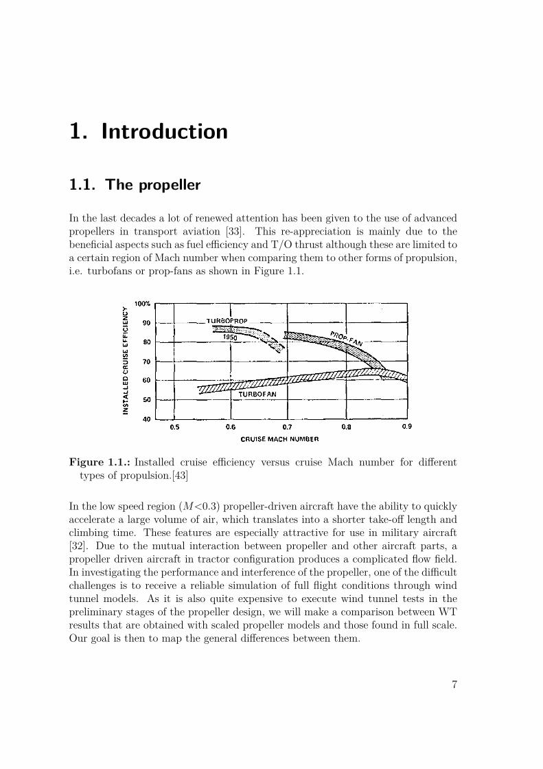
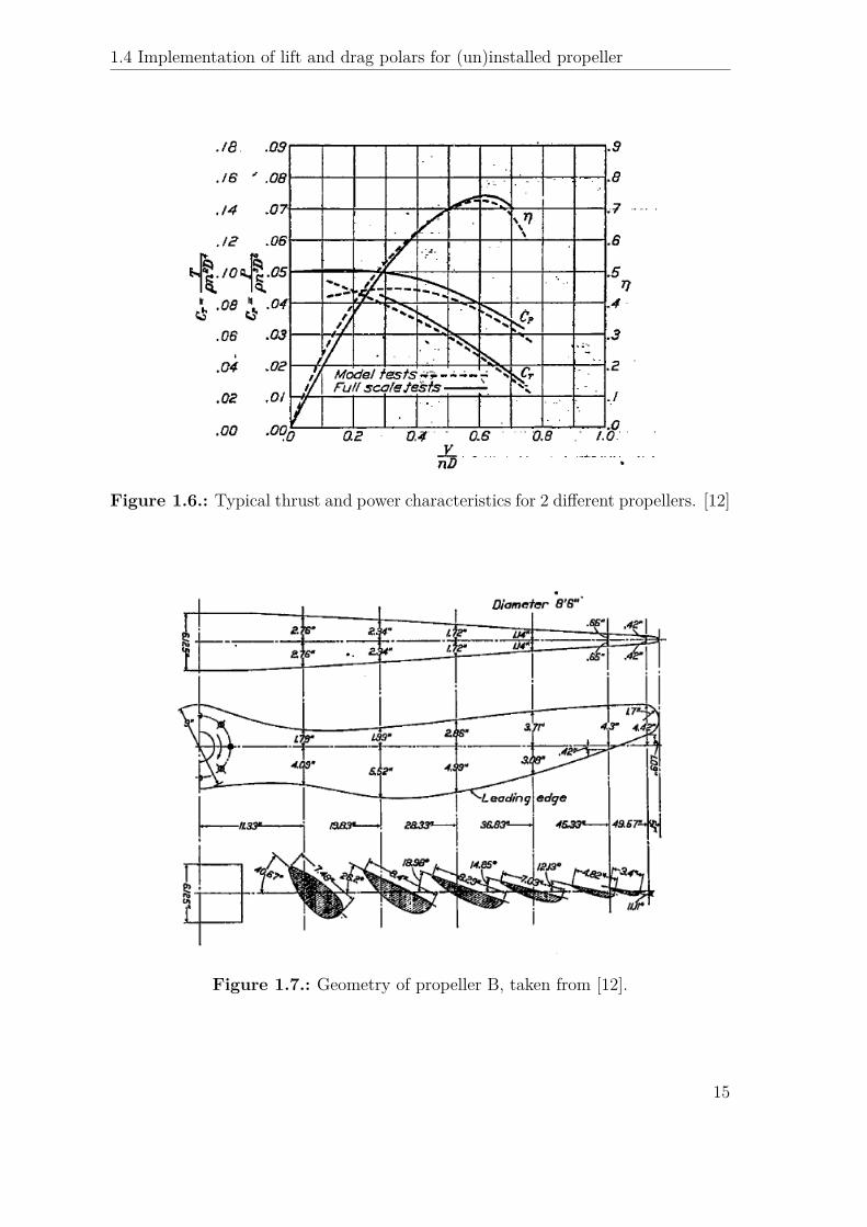
Beginning with some general thoughts, the report of Lesley [12] pointed out that thescaling effect is the reason for the difference between thrust and power of propellersfor the full scale and model. The increase in lift for the full scale propeller sections issuch as to increase the power and thrust as noted in Figure 1.6. The correspondingspecifications can be seen in Figure 1.7.
In recent years several studies were made on the influence that low Reynolds num-bers (<3×10⁵) have on the (propeller)performance of UAV, which could give a goodindication on the models used for real aircraft. Although geometrical characteristicsplay a role, general conclusions for propellers can be made on their use and limi-tations concerning the topic of scaling. An investigation on propellers designed for
14
1.4 Implementation of lift and drag polars for (un)installed propeller
Figure 1.6.: Typical thrust and power characteristics for 2 different propellers. [12]
Figure 1.7.: Geometry of propeller B, taken from [12].
15

Chapter 1 Introduction
Rec >106 [51], confirmed the fact that characteristics became worse with decreasingRec and even unworthy of using them for the lowest regime of Rec(<105). Here, theoption of redesigning propellers for low Rec to give better resemblance with flighttest, is not a useful solution. In [52] the question was raised if performance tests ofmodels could give accurate representation of the full scale. As a change in tip speedwould alter the rotational speed and centrifugal forces on the blades, the question ofRe is much more complicated for a propeller than for a wing since now the Re willvary along the blade. This variation, that is more profound at lower speeds when therotational component dominates the relative velocity, is unimportant at full scale.For the models however, it is likely that the influence of the Re should be dividedinto the “root effects” and the well-known airfoil effects. At the hub, Himmelskamp[53] showed that better airfoil performance was found due to the delay of separationto larger angles of incidence which meant that a lower Rec was possible. He noticedthat the blade rotation would affect the lift polar in such a way as to delay stall andachieve higher maximum lift values. This effect was more pronounced towards theroot due to the lower rotational velocities. The reason is that significant radial flowcan only develop in regions of retarded flow such as separated regions. The flowthat develops in radial direction, due to the centrifugal forces in the boundary layerof a rotating blade, will result in a Coriolis force that acts as a favorable pressuregradient. This leads to a delay of the boundary layer separation and i.e. to higherlift coefficients [11]. Figure 1.8 shows the increased lift coefficients that are obtainednear the hub.
One could conclude that the incorporation of the Himmelskamp effect is justifiedfor every propeller. Further on in the report, it is seen that this is not the case. Anexplanation for this observation is made in chapter 4.
Figure 1.8.: Local lift coefficient at various radial sections on a rotating propeller.[53]
16

1.4 Implementation of lift and drag polars for (un)installed propeller
Tests were conducted to investigate the effect of scaling on the behavior of propellermodels [52]. It was concluded that models used for performance simulation of thefull scale, should not be run well below 5×10⁵ as the efficiency fell dramaticallyunder 3×10⁵. A very important and interesting way of analyzing the Re of propellermodels was given by Lerbs [46] in relating the lift coefficient of the profile to thethrust coefficient and the measured efficiency to the drag coefficient. He made ageneral analysis where he defined the Re based on the fact that above its value thefrictional coefficient of the profile can be deduced from the one of a turbulent flatplate according to a predetermined relation and that at the same time the angle ofzero lift of the propeller profile still coincides with the one of the isolated profile,calculated from potential theory. Drag reduction is one of the effects of Reynoldsnumber increase and this drag is mostly accounted for by the skin friction Thismakes the use of theoretical skin friction drag in Lerbs analysis fairly acceptable[54].
A less clear image is observed w.r.t. the lift coefficient because of the difference inzero lift angle at low Reynolds numbers. Using the hypothesis that the vibration ofthe rotating propeller provides turbulence, it was shown [45] that a rapidly rotatingsmall propeller approaches the full scale condition more accurately than a slowlyrotating large propeller. Still however, the difference in the zero lift angle gives adeviation of the effective pitch angle of a few degrees between the model and fullscale [45]. Using this, Lerbs found good agreement between FS and WT tests atRec ∼ 0.77×10⁶. More important he observed that tests with Rec below 3×10⁵
are expected to give results considerably different than the ones for the full scalecondition.
1.4.2. Propeller integration effects
In the current interest for the use of propellers not only the direct effects on thepropeller performance are important but even more are the effects of the alreadymentioned scaling issues on parts laying in the wake of the propeller. Therefore,an investigation is needed on how the slipstream is altered by these scaling effectsand how this in turn may change the different characteristics of parts behind thepropeller, more specifically on the wing.
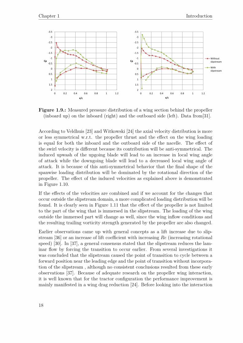
Focusing on the immersed part of the wing in the slipstream, we see that through avariation in slipstream, the characteristics of the wing will change. Considering nowa rectangular, symmetric, untapered and untwisted wing, it is known from theorythat the lift distribution at an angle of attack has an quasi-elliptic shape. Whenthe propeller slipstream is introduced, a change in the lift distribution is observed.Inside the slipstream the axial velocity increases, leading to an increase in dynamicpressure. This implies that the local angle of attack will change and therefore theforces on the wing. An illustration of these changes in wing characteristics is shownin Figure 1.9 and Figure 1.10.
17
Chapter 1 Introduction
����
��
����
��
����
��
����
�
���
�
���
�
� ��� ��� �� �� � ���
��
���
����
��
����
��
����
��
����
�
���
�
���
�
� ��� ��� �� �� � ���
��
���
�� ���
����� ����
�� �
����� ����
Figure 1.9.: Measured pressure distribution of a wing section behind the propeller(inboard up) on the inboard (right) and the outboard side (left). Data from[31].
According to Veldhuis [23] and Witkowski [24] the axial velocity distribution is moreor less symmetrical w.r.t. the propeller thrust and the effect on the wing loadingis equal for both the inboard and the outboard side of the nacelle. The effect ofthe swirl velocity is different because its contribution will be anti-symmetrical. Theinduced upwash of the upgoing blade will lead to an increase in local wing angleof attack while the downgoing blade will lead to a decreased local wing angle ofattack. It is because of this anti-symmetrical behavior that the final shape of thespanwise loading distribution will be dominated by the rotational direction of thepropeller. The effect of the induced velocities as explained above is demonstratedin Figure 1.10.
If the effects of the velocities are combined and if we account for the changes thatoccur outside the slipstream domain, a more complicated loading distribution will befound. It is clearly seen in Figure 1.11 that the effect of the propeller is not limitedto the part of the wing that is immersed in the slipstream. The loading of the wingoutside the immersed part will change as well, since the wing inflow conditions andthe resulting trailing vorticity strength generated by the propeller are also changed.
Earlier observations came up with general concepts as a lift increase due to slip-stream [36] or an increase of lift coefficient with increasing Re (increasing rotationalspeed) [30]. In [37], a general consensus stated that the slipstream reduces the lam-inar flow by forcing the transition to occur earlier. From several investigations itwas concluded that the slipstream caused the point of transition to cycle between aforward position near the leading edge and the point of transition without incorpora-tion of the slipstream , although no consistent conclusions resulted from these earlyobservations [37]. Because of adequate research on the propeller wing interaction,it is well known that for the tractor configuration the performance improvement ismainly manifested in a wing drag reduction [24]. Before looking into the interaction
18

1.4 Implementation of lift and drag polars for (un)installed propeller
Figure 1.10.: Change in the local lift coefficient due to the axial(left) andswirl(right) velocity in the slipstream for an untapered wing. The effect outsidethe slipstream is left out [23].
Figure 1.11.: Lift distribution as affected by the combined effect of the axial andtangential velocity [23].
19

Chapter 1 Introduction
with respect to scale effects, it is important to keep the well know effect of lowReynolds numbers on isolated wings in mind. Studies, as mentioned in the previoussection, showed the dominant problem of a laminar separation bubble and othertypical phenomena at lower Reynolds numbers. A recent and useful investigationconcerned the effect of the propeller slipstream on both the separation bubble andtransition process at low chord Reynolds number [55]. An important aspect is themechanism by which the slipstream is introduced into the boundary layer of thewing. In this work the periodic turbulence, introduced by the propeller, is seen asuniformly distributed along the whole cycle in order to investigate the global effectof slipstream on transition on the wing. This behavior resulted in regions of turbu-lent packets between which the boundary layer seemed to remain laminar. One ofthe conclusions was that the transition mechanism associated with laminar separa-tion bubble was changed to a classical transition process associated with increasedReynolds number and that transition moved towards the leading edge. As noted in[55], the lack of the incorporation of this cyclic behavior into earlier studies couldmake previous conclusions about the flow over the wing in the slipstream incorrect.This was incorporated in [37] since the laminar boundary layer within the slipstreamwas seen as a boundary layer with a cyclic variation of external flow turbulence. Thisexternal flow turbulence is the viscous wake from the propeller blade. Seen from thedisturbance model in Figure 1.12, the turbulence near the surface will remain sometime after the passage of the external turbulence. In this work [55] and others, likefor example Howard R.M. [56], the time-dependent cycle of transitional behaviorin the wing boundary layer was studied. He observed that its characteristics weresimilar to relaminarized flow and laminar flow with external turbulence. More inparticular the drag values at low Re showed that the propeller slipstream enhancesthe stability of the boundary layer and reduces the drag coefficient in the laminarportion of the slipstream cycle below its undisturbed value[56],[37].
Figure 1.12.: The effect of a passing slipstream on the boundary layer flow overan airfoil. [37]
20

1.5 Opportunity for further research
1.5. Opportunity for further research
It is clear from previous sections that a lot of work has been done on both unin-stalled and installed propellers. The issue of scaling on the other hand is a veryimportant topic that needs further investigation. In order to understand the logicin the different steps of this report, listed in the next section, a statement will bemade to explain how this topic of research (scaling effects) will be investigated. Thisstatement will be formulated in a main objective and some fundamental questions.Research questions
• What is the effect of scaling on propellers in wind tunnel tests (i.e. performanceand slipstream)?
• What is the influence of scaling on propeller wing interaction due to changesin the propeller slipstream?
Different sub-questions emerge when a thorough investigation is done on these re-search questions.
• Are the general known limits of values under which resemblance between datais lost actually correct? This merely focuses on the lower limit of the Reynoldsnumber that is generally used in order to be sure that resemblance betweenfull scale and experiment is still present.
• What role do parameters like Mach and Reynolds number have on importantaerodynamic parameters, i.e. on lift and drag?
The fundamental work for understanding the background of these problems, i.e. thesub-questions, was shown in the previous sections. The objective can now be statedas follows.Thesis objective
• Investigate, through the use of theoretical prediction codes, how scaling effectswill alter the propeller performance and the slipstream and i.e. how the flowover the wing is changed as a consequence of this alteration.
1.6. Set up of the report
This report will be build up in the following way. First of all a subdivision is madeinto the four upcoming chapters.
• Chapter 2: Background• Chapter 3: Preliminary survey• Chapter 4: Analysis of uninstalled propeller• Chapter 5: Interference effects of installed propeller
21

Chapter 1 Introduction
• Chapter 6: Conclusions and recommendationsIn Chapter 2 the background theory concerning propellers is stated together withthe useful terminology in order to have an idea about the basics needed for a goodunderstanding of the following work.Chapter 3 handles the description and verification of different theoretical predictioncodes that are available for propellers. A short description of the selected predictionprogram is given after which we will try to investigate how well reference data canbe represented in the programs. This is done by taking data from open literaturewhere investigations on propellers were performed and comparing them with datafound in the program on similar propellers.Chapter 4 will take a deeper look into the representation and effect of the Reynoldsnumber in the selected program. In a second stage, this program will be used to val-idate data from papers and investigate how this data is translated in to parameterslike for example the induced velocities of the propeller.In Chapter 5, an investigation is performed with a propeller interaction program tosee how the results from Chapter 4 will affect the wing. In other words, an attemptwill be made to provide the reader with consistent information on how the differentdata of the propeller in full scale and wind tunnel will influence the trailing wing.At the end, an analysis is made to see other effects on the lift distribution, like forexample the position of the propeller.Finally, Chapter 6 contains the conclusions that were drawn and the recommenda-tions for future work.
22

2. Background
2.1. Propeller theory
In order to have a clear view on every (sub)topic that will be tackled, a short recapof theory and terminology needs to be established. Throughout this work, someinformation will be added to clarify specific questions like transition, interferenceeffects and more.
2.1.1. Propeller concept
Propeller blades can merely be seen as wing sections producing an aerodynamicforce but because of their different application a rotational velocity is added to theforward velocity of the blade flight path resulting in a helical flight path. Since theaerodynamic forces are presented as torque and thrust, a good understanding ofthe relation between them and the forces on the wing, i.e. lift and drag, is needed.Although the forward velocity over the blade is assumed constant, the rotationalvelocity will depend on the blade section and α will vary accordingly.Propellers operate most efficiently if the α is constant over the larger part of theblade (giving the best Cl/Cd ratio for propeller efficiency). For this reason twist isused throughout the blade length.
2.1.2. Propeller aerodynamics
In order to analyze the aerodynamic performance of a propeller by means of a model,different theories can be applied. As a propeller produces thrust by forcing air be-hind the aircraft, it will produce a slipstream. It can then be crudely considered asa cylindrical tube of spiraling air propagating towards the rear over the wings. Inanalyzing a propeller model, different approaches can be used in a compatible way;using the blade element theory to predict the propeller forces and the momentumtheory to relate the flow momentum at the propeller to the one of the far wake. Thereason that these two theories are combined is as follows. In dealing with propellerperformance, momentum theory based on the hypothesis of a stream tube enclosingthe complete propeller disk, is a simple and classical used method. Because this the-ory does not provide enough accurate information to find meaningful relationships
23

Chapter 2 Background
between the different blade parameters, blade element theory is often used instead.Combining the results of these two analyzes, relations are found for the differentialpropeller thrust and torque. For this analysis a clarification of the models is needed.
Momentum theory
This work, introduced by Froude and continued by Rankine, is based on the followingassumptions:
• The flow is inviscid• The flow is incompressible• There is no rotational motion of the flow in the slipstream• Both the velocity and the static pressure are uniform per unit disk area
Figure 2.1.: Propeller stream tube indicating the freestream velocities and radiusat different axial positions. [35]
This means for the axial direction that the change in flow momentum along a stream-tube starting upstream, passing through the propeller, and then moving forward intothe slipstream must equal the thrust produced by this propeller [35].
T = ρπR2sVs(Vs − V∞) (2.1)
The second implication is that for each cross section the pressure jump over the discshould be equal to the thrust [41].
24

2.1 Propeller theory
T = (p+ − p−)A (2.2)
Application of Bernoulli’s equation both up- and downstream of the disk leads tothe following:
p+ − p− = 12ρ(V 2
s − V 2∞) (2.3)
Combining these equations with the continuity condition results in the proof thatthe velocity through the disk is equal to the average of both the up- and downstreamvelocities.
V = V∞ + Vs2 (2.4)
Blade element theory (BEM)
In the above theory of momentum there are not enough equations given to comeup with the expression for the differential propeller thrust and torque of a givenspan location. The additional equations that can be used are dependent upon thestate of the flow. This flow state is dependent on the characteristics of the propellerblades. These geometrical properties are used in blade element theory in order todetermine the forces that the propeller exerts on the flow field. As we are dealingwith finite elements, the blade is split into a number of distinct section of widthdr. For each element the blade geometry and flow field properties are then relatedto a differential propeller thrust dT and torque dQ. This is done by making twosupplementary assumptions [35]:
• In the analysis, no interaction is present between the blade elements• The forces exerted on each blade element by the flow are purely determined
by the two-dimensional lift and drag characteristics of the blade elementIn determining the aerodynamics forces that result on the blade elements, it is helpfulto look at the velocity diagram as given in Figure 2.2. The inflow angle based uponthe two components of the local velocity vector is found to be:
tanϕ = tan(ϕ′ + αi) = V∞ + Vaωprp − Vt
(2.5)
25

Chapter 2 Background
By looking then at Figure 2.2 the following relation is apparent:
Ve = V∞ + Vasinϕ1
(2.6)
The induced velocities are function of the forces on the blades and the combinationof both theories is used to calculate them.Finally with the aid of this figure the thrust around an annulus of width dr isequivalent to:
dT = 12βρV
2e (Clcosϕ− Cdsinϕ) cdr (2.7)
and the torque for each annular section is given by:
dQ = 12βρV
2e (Clsinϕ− Cdcosϕ) crdr (2.8)
Figure 2.2.: Velocity diagram of a blade element. [28]
26

2.2 Interference effects
From Equation 2.7 and Equation 2.8 we see that for this model the Re numberdirectly influences the thrust and torque through the blade airfoil lift and dragcoefficient. Therefore the Re number dependency of the lift and drag polar form acrucial part of the investigation.
2.2. Interference effects
The flow field of an isolated propeller and an installed propeller differ significantlyfor reasons that will be explained in this section. It is important to note thatwe are working with a propeller in tractor configuration. This means that thepropeller is situated upstream with respect to the wing. It is evident that theunderstanding of this topic is very important as the propeller slipstream influencesboth the performance and aerodynamic behavior of the wing. On the other handthe upwash induced by the wing influences the flow field of the propeller blades. Itchanges the local angle of attack of the propeller blades similar to an uninstalledpropeller subjected to an angle of attack as can be seen in Figure 2.3. The effectivevelocity experienced by the downward rotating blade is increased by the wing’supwash, which leads to a local angle of attack increase. This results in an increasein elemental lift and blade loading, which augments the thrust and torque on theblade. The upward rotating blade on the other hand experiences a decrease in thelocal angle of attack leading to a decreased elemental lift and blade loading. Thusthe upward rotating blade experiences a decrease in thrust and torque.
Figure 2.3.: Effect of wing’s upwash on the propeller blades. [32]
In the case of the tractor configuration, the wing experiences swirl velocities thatinitiate from the propeller and result in a deformation of the lift distribution [29].
27

Chapter 2 Background
By using numerical and experimental methods, it was found that the propeller-winginteraction effects for certain tractor propeller configurations resulted in significantwing drag reduction [32]. The interaction between the wing and the propeller isprovided by the velocity field induced by the lifting line within the propeller’s streamtube and by the velocity field induced by the propeller slipstream on the lifting line.The former will affect the power characteristics of the propeller and the latter willyield the change in wing induced drag [17]. Just as wings can be modeled by vortexline theory, propellers can be modeled by a series of helicoidal vortex sheets. As weare only interested in the overall performance and the effects induced on the wing,this model can be simplified to a vorticity tube model [17]. Through the use of thismodel, the induced velocities i.e. the axial and swirl component can be calculatedand are represented below in Figure 2.4.
Figure 2.4.: Induced velocities by propeller vorticity tube. [17]
Although there is also a third velocity component in practice, the radial component,the incorporation of it is often left aside as it is small compared to the other inducedvelocities. As mentioned before, the induced velocities will alter the behavior andperformance of the wing. Several studies like the one on the F-50 [31] investigated theeffect of the slipstream on the wing by changing the thrust coefficient. The result wasa change in the dynamic pressure and swirl angle, i.e. the local angle of attack. Thescaling effect on these parameters is an important topic to keep track of. Anotheraspect that plays an important role in altering the performance is the inclinationand position of the power plant with respect to the wing. In [30] it was found that avertical movement of the propeller towards the wing would produce higher lift than achange in longitudinal direction. Pitching down the propeller/nacelle enhanced thelift performance even more than a vertical or horizontal variation and showed thepowered wing to be more sustainable to higher angles of attack near maximum lift.
28

2.3 Terminology
Although it is wise to keep this aspect in mind, it does not belong to the core of ourproblem as we best focus on scaling effects in a certain configuration (conventionalwithout inclination).
2.3. Terminology
In this work different definitions will be used to characterize the propeller aero-dynamics. As previously mentioned, the torque and thrust force can be found bydecomposing the lift and drag forces onto the axis of rotation and the plane of rota-tion respectively. Another way of expressing them is by using the non-dimensionalcoefficient, as is done in our case:
• Thrust coefficient
CT = T
ρn2D4 (2.9)
• Torque coefficient
CQ = Q
ρn2D5 (2.10)
• Power coefficient
CP = P
ρn3D5 (2.11)
• propeller efficiency
η = TV∞P
(2.12)
These coefficients can also be expressed by using the non-dimensional advance ratioJ . This parameter gives the ratio of the distance V∞
nthat the aircraft moves per
revolution to the propeller’s diameter D.
J = V∞nD
(2.13)
29


3. Preliminary survey
3.1. Available propeller programs
Before starting the investigation on scaling effects in propeller testing, a verificationof different propeller programs is needed in order to see if there is an acceptableprogram available that can give good resemblance between data from wind tunneltesting. Different reports will be used as reference and their results (i.e. CT versus J)will be compared with the ones we get from the specific propeller prediction program.At the end a preference should then be made about which calculation approach andprogram serve best for the purpose of representing scaling effects on propellers. Animportant aspect is how accurate the effect of Rec on propeller performance can berepresented. As for all investigations where we want to analyze a certain effect, onlyone parameter may vary in time. In our case the change in thrust coefficient CT fora constant advance ratio J will be used for the visualization of this effect. Since itis needed to implement the effect that Reynolds number has on the propeller, welimit ourselves to the application of Blade Element Methods (BEM).
3.2. Programs
3.2.1. PropCalc
PropCalc is a program, based on the blade element theory, that only needs a largeamount of parameters to specify the design. BEM, as already mentioned, is a methodwhere the blade is divided into small sections, which are handled independently fromeach other. Each segment has a chord and a blade angle and associated airfoil char-acteristics. The theory makes no provision for three dimensional effects, like sweepangle or cross flow. But it is able to find the additional axial and circumferentialvelocity added to the incoming flow by each blade segment. It offers a large edibilitywhen specifying the data, which makes this program very useful. The lift and dragpolars for example, are represented by specifying each data point separately. Fur-ther information can be found in [2]. One of the drawbacks is the limitation in Re:values above 1×10⁶ can’t be applied as the program only works with values up to5 digits. This problem can actually be avoided by filling in lower values for higherpolars. In this way, the effect of Re can still be visualized. A comparative study willbe made with several reports, from which the most important features can be found
31
Chapter 3 Preliminary survey
in table 3.1. The reference data from the reports and the data from the programi.e. CT versus J can be found in Appendix A. Our main goal is to look how well thereference data is attained with the use of the program. The results can be found inthe next section, in order to make the comparison with the last program that willbe discussed.
Report 640[3] Report 378[4] TN 1111[5] Report 712[6]Diameter�[m] 3.05 2.89 3.72 1.22
Number of blades 3 2 2 2β at 0.75R [deg.] 35 19 29.2 32Airfoil section Clark Y Clark Y Clark Y NACA 4412
Table 3.1.: Specific features of propellers used in different reports.
3.2.2. Qprop
In Qprop, the analysis of the propeller is based upon an extension of the bladeelement theory and the incorporation of vorticity. In vortex theory, circulation ispresent around each blade. This circulation vanishes towards the tip and root.The blade may be replaced by a bound vortex system which, for simplicity, canbe approximated by a bound vortex line. It was stated that if the distributionof the strength of the vortex along the blade, equal to Γ, is such that the energylost per unit time is a minimum for a given thrust, then the flow far behind thescrew is the same as if the screw surface formed by the trailing vortices is rigid andmoved backwards with a constant velocity. In this case the circulation round anyblade section is equal to the discontinuity in velocity potential at the correspondingpoint of the screw surface. With this statement, a calculation can be made forthe circulation distribution by solving the potential problem of the screw surface.The complete elaboration can be found in [57]. It only uses a simple linear Cl-linewith minimum and maximum values. For the drag characteristic a limited amountof values is used, which are fitted to form a quadratic function. An explanationof these techniques will be given in section 3.4. One would assume that because ofthese approximations, the result would be less accurate than with PropCalc, but theopposite is true as can be seen later on. More background information is given in [7].Data obtained from Qprop can also be found in appendix A, together with the otherdata. Care has been taken that geometry, sections and blade angle distribution arethe same for both programs with respect to the different reports. The results canbe seen in Figure 3.1 through Figure 3.4.
32

3.3 Validation of the programs
3.3. Validation of the programs
With the aid of the information in table 3.1 and the polars that characterize thespecific airfoils, the performance characteristics can be drawn by using the differentprograms. These polars can be found in the relevant papers or in airfoil databases[3, 4, 5, 6]. Several known experimental data sets are used to see what kind ofgeneral results can be expected.
We see that there is a good representation of the experiment in both Qprop andPropCalc for higher J , but the curve starts to break down on the left side. However,it can be seen that the results from Qprop give a better fit with the experimentthan the ones from PropCalc. In the thesis of Momchil Dimchev [8], the focus forcomparison was put on the later linear part of the curve. He concluded that Qpropgave a close match with experimental results while at lower J the results start todiverge considerably. A possible explanation is that this region is characterized bythe onset of flow separation and cannot be handled accurately by BEM. It is one ofthe reason that we will focus on higher J for our further research. Another reasonis that the literature, like the one from Dimchev, also focuses on these higher J . Asan illustration, the results from Dimchev’s thesis can be seen in Figure 3.5.
�
����
����
����
����
���
����
����
����
����
� ��� � ��� � ���
��
�
�����
�������
���� ����
Figure 3.1.: Comparison of thrust coefficient CT versus advance ratio J with ex-perimental values attained from [3].
As a result, the exact same conclusion can be drawn in our case: Qprop gives a verygood match with the experimental results, which is better than the results obtainedfrom PropCalc.
33

Chapter 3 Preliminary survey
�
����
����
����
����
���
� ��� ��� ��� ��� � ���
��
�
��
�� ��
���������
Figure 3.2.: Comparison of thrust coefficient CT versus advance ratio J with ex-perimental values attained from [4].
�
����
����
����
����
���
����
��� ��� � ��� ��� ��� ���
��
�
�� ��
�������
��
Figure 3.3.: Comparison of thrust coefficient CT versus advance ratio J with ex-perimental values attained from [5].
34

3.3 Validation of the programs
�
����
����
����
����
���
����
� ��� ��� ��� ��� � ��� ��� ��� ���
��
�
��� ��
���������
����
Figure 3.4.: Comparison of thrust coefficient CT versus advance ratio J with ex-perimental values attained from [6].
Figure 3.5.: Thrust coefficient versus advance ratio for two propeller blade angles.Figure from Dimchev[8]
35

Chapter 3 Preliminary survey
3.4. Set up of selected prediction program
Based on the results of the comparison between experiment and the different pro-peller programs, Qprop was chosen as a prediction program for our further research,since a better match is found with the experiments.
3.4.1. Theory of Qprop
Flow velocities
In a first instance, the axial and tangential components (Va, Vt) of the resultantvelocity Ve are decomposed with the aid of Figure 2.2. Then a relation is madebetween the total circulation over all the blades (BΓ) and the local swirl velocity.The total derivation of the velocities is given in [62]. The formula for Vt is given asfollows:
Vt = BΓ4πr
1F
√1 + (4κwR/πBr)2
(3.1)
And assuming that vi is perpendicular to Ve, we can write Va as follows:
Va = Vt(ωr − Vt)(V∞ + Va)
(3.2)
Blade geometry and analysis solution
The local lift and drag coefficients are calculated together with the local blade cir-culation. The blade circulation for a local lift coefficient and local chord length isdefined as follows:
Γ = 12Veccl (3.3)
The input file contains the blade geometry (c, β), blade airfoil properties (cl, cd) foreach radius, and operating variables V∞ and rotational rate. With this information,the radial circulation distribution Γ(r) can be calculated for each radius indepen-dently. This is performed by solving the preceding nonlinear governing equations
36

3.4 Set up of selected prediction program
via the Newton method. In this method, the solution is approximated by iteratingover a certain function with a predetermined value of the solution. Rather thaniterating on Γ directly, it is beneficial to instead iterate on a the dummy variable.This dummy variable parametrizes all the other variables.
Thrust and Torque relations
After applying the Newton method for each radial station, the overall circulationdistribution is known. This then allows the calculation of the overall thrust andtorque of the rotor. The total thrust and torque are obtained by integrating thelocal thrust dT and local torque dQ as defined in the previous chapter.
Analysis
The analysis problem contains the determination of the loading on a rotor of givengeometry and airfoil properties, with some suitable imposed operating conditions.We still have 4 unknowns (Γ, V∞, RPM, β). The constraints on Γ(r) are the Newtonresiduals defined as:
<(Γ(r)) = Γ− 12Veccl (3.4)
The other unknowns are specified at the start of the analysis. The three residualsthat constrain these unknowns are then simultaneously driven to zero in the Newtoniteration method.In Figure 3.6, a flow diagram is given for clarification. It contains the different stepsof the theory as explained in this section. The input for Qprop consists out of twoparts. One includes the specifications for the blade geometry, number of blades,diameter and the lift-drag polars. In the other part, the three remaining unknownsare specified.
3.4.2. Data input
3.4.2.1. Definition and measurement techniques
By requiring a rather detailed description of the propeller input file, Qprop is ableto accurately capture the propeller’s performance. In this file the geometry canbe specified for up to ten radial positions together with the number of blades anddiameter. For the drag and lift polar, a specific technique is used to prescribethe aerodynamic characteristics. In Figure 3.7, it is seen that for the drag polar aparabolic fit is used and a linear fit for the lift polar. After implementation of thefitting technique, the different parameters needed for the input file can be derived.
37

Chapter 3 Preliminary survey
Figure 3.6.: Flow diagram for the analysis part of Qprop.
Figure 3.7.: Parabolic and linear fitting of the drag and lift polar respectively, inorder to represent the aerodynamic characteristics of the blade section airfoils[34].
38

3.4 Set up of selected prediction program
3.4.2.2. Reynolds influence
Qprop uses a parabolic fit for the drag polars, which could imply that the effect of adrag bucket with irregular shape becomes harder to represent in the program. Thispossibility is of less importance due to the fact that the irregular shapes are mostlycharacterized by extreme low Re as seen in Figure 1.4. The general influence of anincreased Reynolds number on the drag polar, as mentioned in section 1.3, is mainlyseen in a wider drag bucket and less in a reduction of the minimal value of the dragcoefficient (i.e. a lower drag bucket) when comparing the WT to the FS case. Inthe next chapter this conclusion can be confirmed when a representation is made ofthe Reynolds variation.The influence of the Reynolds number on the linear fit of the lift polar is much morepronounced: increasing Re results in a higher maximum lift coefficient, slope andzero angle of attack. These are three direct inputs in the input file. In will be seenonce more in the next chapter that the Re influence of the lift polar has more effecton the performance calculations than the one of the drag polar.
39


4. Analysis of uninstalled propeller
4.1. Reynolds variation and limitations
First and foremost, we want to know how well typical wind tunnel tests can sim-ulate the propeller performance data of the full scale. It is therefore important tovalidate how these characteristics are influenced by Re variation. It was stated insection 2.1 that when different propeller theories are combined, a clear relationshipexists between thrust and torque and some fundamental coefficients. It also explainshow coefficients like the lift and drag polar are influenced by the scale effect. Thisis the reason that in the following investigation different polars will be used andcompared in the program. In this chapter a validation is made on the influenceof the Reynolds effect in the propeller program. What follows is the incorporationof possible improvements to the chosen program. By doing so, we will be able tohave a better understanding of the errors between full scale and wind tunnel tests asaffected by differences in Reynolds number. In a next stage, an investigation is doneon what this means for other areas of interest, i.e. the slipstream and the wing.
4.1.1. Re influence on propeller characteristics
In the previous chapter the choice was made to take Qprop as a standard referencepropeller program since it turned out to have the best resemblance with knownWT test data. Another aspect that we would like to investigate is how well theReynolds variation is translated in the characteristics of propellers. In order to dothis, the polars will be altered in Qprop as if they were affected by the Reynoldsnumber. The results show that the errors in similarity between experiment andfull scale become marginal when we increase the Rec (> 5− 7×10⁵) [18],[44]. Thisvalue, as mentioned before, is taken at r = 0.75. Unfortunately a difference remainsw.r.t. the corresponding full scale Reynolds number as the lift characteristic of thesehigh values (> 1×10⁶) is not reached yet. The reason being that the resistanceto separation of the turbulent boundary layer increases due to a reduction of theskin friction with increasing Rec. Note however that this improvement will occurmore slowly when reaching higher values, i.e.> 1×10⁶ [18]. In representing the Reinfluence, we need to bare in mind that in general the lift decreases both in slopeand maximum value with decreasing Rec. On the other hand, the drag coefficientincreases, mostly on the ’sides’ of the drag bucket. This can be seen with the aid of
41

Chapter 4 Analysis of uninstalled propeller
Figure 1.4 and [9]. In [9], different polars are given for specific Reynolds numbersand the influence on the performance characteristic can be seen in Figure 4.1, withthe aid of Qprop. The geometry of the propeller is given in Table 4.1[1]. The polarsfrom [9] are used and can be seen in Figure 1.4.
�
����
���
����
���
����
���
��� ��� ��� ��� ��� ��� ��� ���
��
�
������
����
������
������
Figure 4.1.: Propeller performance characteristics affected by different Rec num-bers.
rR
0.2 0.3 0.4 0.5 0.6 0.7 0.8 0.9 1.0chord [mm] 25 51 77 91 99 100 92 72 3β [deg.] 79 73 67 62 57 52 48 45 42
Diameter�[m] 2.2Number of blades 6
Table 4.1.: Geometry of propeller used for the representation of Rec effect.
In this particular case, the influence of Reynolds number remains small since thedifferences between the polars are also rather limited. In Figure 4.3, we take thecase where the Rec is equal to 1.72×10⁵ and make visible adaptions to the polar inorder to see the influences on the performance characteristic. These adaptations arebased on data, found in [9]. Here, different polars are given that are characterized bydifferent values of Re for typical (propeller) sections. It then becomes easier to seethe influences of the polars on the performance characteristic. These adaptationsare illustrated in Figure 4.2.
From Figure 4.3, it becomes clear that the main differences are caused by a changein the maximum lift coefficient and lift slope. We can then assume that the liftadaptations have the most influence in Qprop, although a change in drag polar canstill cause some changes.
42

4.1 Reynolds variation and limitations
�
���
�
���
�
���
��� ��� ���� ���� ���� ���� ����
��
�
��
�� �����������
���������������
�
����
����
����
����
���
� ��� � ��� �
��
��
�� �� � ���
�����
�� ��� ���
�����
������ ���
�����
Figure 4.2.: Different type of adaptations in the lift and drag polars.
�����
�����
�����
�����
�����
�����
��� ��� ��� ��� ��� ��� ��� ���
��
�
�� �����
�������������
�������������
������ �� !
!"�#�� ����
Figure 4.3.: Influence of polar adaptations on the propeller performance charac-teristic with reference case, Rec equal to 1.72 ×10⁵.
43

Chapter 4 Analysis of uninstalled propeller
4.1.2. Improvements
In chapter 3, Qprop was chosen because of its good representation of experimentaldata. For low advance ratios however, it was explained that the difference withtest data was significant and not even representable. Different flow phenomena thatcharacterize propellers are not included in the program since we only use a basicmodel. One can anticipate that building the effect of these phenomena into theprogram will possibly lead to an improvement for the higher advance ratios.
4.1.2.1. Stall delay
One of the phenomena that was first observed by Himmelskamp [10] was a rota-tional effect called stall delay. An explanation of this phenomena, characterized byan increase in lift curve, was given in the introduction. Several general rules havebeen made to represent this increase in lift coefficient. In [61], different correctionmethods were analyzed in order to include the rotational effects on aerodynamiccoefficients. Although similarity was found, some methods needed insight in theamount of rotational augmentation or depended strongly on the maximum lift co-efficient. Therefore, the correction model of Snel, Houwink and Bosschers was used[11]. In their model, the correction is proportional to ( c
r)2:
Cl,rot = Cl,2D + 3(cr
)2(Cl,pot − Cl,2D) (4.1)
To put this improvement to the test, the correction model was implemented into thedata of some earlier reports. Figure 4.4 shows how this model alters the lift polarfor a specific airfoil-type, i.e. the Clark Y airfoil, used in many of our propeller tests.The correction was applied up to 60% of the radius since the improvement is verysmall for larger radii, as can be seen in Figure 4.4. The same conclusion was madein [61]. The results that include the implementation of this correction are shown inFigure 4.5 to Figure 4.8.
44

4.1 Reynolds variation and limitations
�
���
���
���
���
�
���
���
���
���
�
� � �� �
��
�
�� ����������
����������
����������
����������
������������
Figure 4.4.: Application of the correction model according to Equation 4.1 for thelift polar of the Clark Y airfoil (viscous flow).
�
����
����
����
����
���
����
��� ��� ��� � ��� ��� ���
��
�
��� ������������
����� ��
��������
Figure 4.5.: Comparison of the Himmelskamp correction in Qprop with experi-mental values attained from [6].
45

Chapter 4 Analysis of uninstalled propeller
�
����
����
����
����
���
����
����
����
����
��� �� ��� �� ��� ��� �� ���
��
�
���������
�����������
��������������
����
Figure 4.6.: Comparison of the Himmelskamp correction in Qprop with experi-mental values attained from [3].
�
����
����
����
����
���
����
��� ��� ��� �� � ��� ��� �� ��� ���
��
�
���������
�����������
������������������
Figure 4.7.: Comparison of the Himmelskamp correction in Qprop with experi-mental values attained from [5].
46
4.1 Reynolds variation and limitations
�
����
����
����
����
���
����
� ��� ��� ��� ��� � ���
��
�
���� � �
���� � ��� ������
��� ��� �
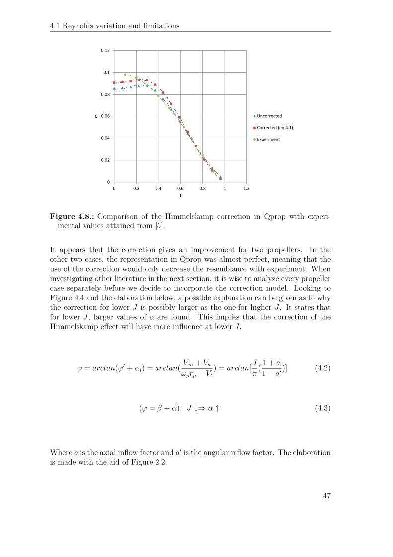
Figure 4.8.: Comparison of the Himmelskamp correction in Qprop with experi-mental values attained from [5].
It appears that the correction gives an improvement for two propellers. In theother two cases, the representation in Qprop was almost perfect, meaning that theuse of the correction would only decrease the resemblance with experiment. Wheninvestigating other literature in the next section, it is wise to analyze every propellercase separately before we decide to incorporate the correction model. Looking toFigure 4.4 and the elaboration below, a possible explanation can be given as to whythe correction for lower J is possibly larger as the one for higher J . It states thatfor lower J , larger values of α are found. This implies that the correction of theHimmelskamp effect will have more influence at lower J .
ϕ = arctan(ϕ′ + αi) = arctan( V∞ + Vaωprp − Vt
) = arctan[Jπ
( 1 + a
1− a′ )] (4.2)
(ϕ = β − α), J ↓⇒ α ↑ (4.3)
Where a is the axial inflow factor and a′ is the angular inflow factor. The elaborationis made with the aid of Figure 2.2.
47

Chapter 4 Analysis of uninstalled propeller
4.1.3. Point of observation
A small observation is made when looking at the analysis of the different reports. InFigure 3.5, a comparison is made between Qprop and references of Dimchev’s thesis[8]. We can see an over- or under scaling between the data depending on the factthat the β angle at 0.75 radius was larger or smaller than a certain value. As a cruderule for this observation, β = 27◦ can be taken. Looking back at the data of Qpropand our reports, we see a similar trend: the Qprop thrust values are over predictedwith respect to the reported test data when β ≤ 27◦ and vice versa. A possibleexplanation for this phenomena could be the Himmelskamp effect. The cross flowcomponent over the blade will increase when β is increased. This leads to a largereffect of the Himmelskamp effect on the flow. The difference between experimentand Qprop for larger β could therefore be caused by the lack of the incorporationof the Himmelskamp effect.
4.2. Validation and investigation with Qprop
In the earlier sections a useful propeller program was put forward in order to havea reliable basis for the investigation. Some improvements and influences in the pro-gram have been explained. The program will now be used to validate the differencebetween the scaled wind tunnel models and the full scale cases. As a next step, wewill investigate the differences in the performance characteristic that are caused bythis offset in data from the different test cases. More specifically, the focus is puton the axial and swirl velocities of the rotor disk and how the results change as aconsequence of the shift between model and full case.
4.2.1. Validation of the propeller performance (WT-FS)
4.2.1.1. Consistent difference between data
In order to do the validation, literature [12] is used where the focus was put onthe comparison of propeller tests between in-flight and wind tunnel models. Thedata will be put in graphs first, followed by a representation in Qprop. The fullscale equipment included five propellers in combination with a VE-7 airplane andthe coefficients of interest were derived according to section 2.3. The model partwas carried out at the aerodynamic laboratory of Standford University and thecorresponding coefficients and elements of performance were directly measured. InFigure 1.7, the geometry was already presented for one propeller.
The representation in Qprop will be done for all five propellers. It can be seen in [12],that the thrust coefficient (but also the power coefficient) for the full scale is about6 to 10 percent larger than the one derived from model tests with a mean around 8
48

4.2 Validation and investigation with Qprop
percent. This difference appears to be too large and consistent to be attributed toexperimental or accidental error [12]. In the paper it is noted that three differentcauses appear for the consistent difference between full scale and model tests.A.The scale effect. It could be stated that this actually represents the Reynoldsinfluence in the tests as an increase in Re tends to increase/shift the lift polar ina beneficial way. This was already mentioned in subsection 4.1.1. The scale ratioof the full-size propellers and the models is 2.72 and the freestream velocity for fullflight is about three times the one for the models. This means that V∞l for thesections of the full flight is about eight times the one for the model. If the formula
ClF S= ClW T
+ 0.057 ∗ logV∞2l2V∞1l1
(4.4)
is applicable, the increase in life coefficient for the full scale sections is such as toincrease the thrust and power about the 8 percent experienced. This formula is theresult of an investigation by Diehl [13] into the effect of changes in size and speedupon the airfoil lift and drag coefficient and it was used in [12] to represent thedifference between WT and FS.Using this adaptation in our formula, good resemblance can be seen in the graphsof the next section.In Qprop we saw that it was merely the lift polar that influenced the change indata when small changes were made, for example under the influence of Reynoldsnumber variation. And again in this paper, only an adaptation in the lift coefficientis prescribed to deal with the scale effect. Yet another indication that this makesup for the bigger part of the deviation between the different data.B.Difference in geometry betweenmodel and full scale. In the case of the model tests,the propeller shaft is parallel and constant to the flight path whereas for the in flighttests the propeller is generally in yaw due to the angle of the propeller shaft. It ap-peared that the effect of this yaw is to increase both power and thrust absorbed.C. Lack of complete similarity betweenmodel and full scale. For the model tests, thetail surfaces and rear portion of the fuselage are omitted. It is observed that atdistances one to one-half diameters of the propeller an effect is produced on thepropeller which stays within the error of observation. On the other side it is foundunlikely that the interference of the slipstream with the tail surfaces would have anyinfluence on the shaft thrust.Knowing that we do not use the data for the combination of propeller and airplanebut only the data for the propeller-alone case, and the geometry is perfectly scaledbetween model and full scale, we do not need to incorporate the effects of B andC as a possible cause. Before doing so, it is wise to investigate the contribution of
49

Chapter 4 Analysis of uninstalled propeller
Himmelskamp and see what effect it has on the match between the data from Qpropand the paper [12]. On the other hand, the Himmelskamp effect doesn’t guaranteethat better data will be found for comparison with this paper.
4.2.1.2. Contribution of Himmelskamp to the validation process
It is evident that a good match for the literature is sought in Qprop. One wouldtherefore assume that the incorporation of the Himmelskamp effect in the data isnecessary. However caution should be paid when making this decision.In the next figures, i.e. Figure 4.9 and Figure 4.10 ,two sets of five different perfor-mance data are given for a specific propeller, i.e. propeller B.Figure 4.9 gives the first performance data set:
• full scale and model case of the NACA paper (Experiment FS & ExperimentWT)
• the data for the model case without Himmelskamp effect which is put in Qprop(Uncorrected WT)
• the data that represent the full scale case in Qprop in theory (Uncorrected FSTheory)
• data for the full scale case in Qprop, which is obtained by using Equation 4.4(Uncorrected FS)
�
����
����
����
����
���
��� ��� ��� ���
��
�
���� � ����
���� � ����
���� � ������� ���
��� ��� ����
��� ��� ����
Figure 4.9.: Comparison of WT and FS case in Qprop with experimental valuesattained from propeller B in [12].
50

4.2 Validation and investigation with Qprop
Figure 4.10 gives the second performance data set:
• full scale and model case of the NACA paper (Experiment FS & ExperimentWT)
• the data for the model case with Himmelskamp effect which is put in Qprop(Corrected WT)
• the data that represent the full scale case in Qprop in theory (Corrected FStheory)
• data for the full scale case in Qprop, which is obtained by using Equation 4.4(Corrected FS)
�
����
����
����
����
���
��� ��� ��� ���
��
�
��� �����
��� �����
��� ����������
�������� ���
�������� ���
Figure 4.10.: Comparison of WT and FS case in Qprop when the Himmelskampeffect is included with experimental values attained from propeller B in [12].
Although Himmelskamp appeared to have a positive effect in some cases of ourprevious investigation, it gives a few unwanted deviations in this case. On onehand, an overshoot is seen for the higher values of the thrust coefficient. On theother hand, for larger values of advance ratio, the differences almost remain the sameas it is merely seen in a change of the slope. Because of the important fact that wefocus on larger values of J and knowing the negative effects such as overshoot and asmall deviation in the slope, we state with certainty that the evaluation of the datacan be done without the incorporation of the Himmelskamp effect. Important tonote here, is that this decision can be different for other investigations, as the focusof interest may differ.
51

Chapter 4 Analysis of uninstalled propeller
Deviation between experiments and Qprop
In the investigation of the five propellers, there is a small difference in the perfor-mance characteristic between the actual values of the paper and Qprop. As thecorrection for the Himmelskamp effect didn’t give the expected improvement, otherreasons should be sought for this lack in resemblance. In what is next to come, apossible explanation is brought forward, based on the only uncertainty in our datainput: inconsistent data for the same type of airfoil. One of the more obvious rea-sons could be the use of incorrect data of the airfoil. More specifically, we focus onthe parameters that characterize the polars in Qprop. When looking at differentpapers as [14],[15] and [59], we come across small differences in the parameters thatare used to characterize the lift polar in Qprop. It is actually the extraction of theaerodynamic characteristics like polars that is not straightforward in Qprop whencomparing it to others. It was noticed in chapter 3, that for other programs thelarge edibility of the data could be very useful. Unfortunately in Qprop a carefulinterpretation of the lift and drag polars is needed since small changes in the valuescan result in unexpected deviations of the propeller coefficients. The main reason,as already mentioned in subsection 3.4.2, is that it uses specified fitting techniquesto determine the aerodynamic characteristics, assuming a parabolic fit for the dragpolar and a linear fit for the lift polar.
The difference in lift polar between literature is certainly seen in the lift coefficientat the zero angle of attack. Looking at paper [59], values of 0.45 and higher arenoticed. It is important to keep in mind that our test data is situated around valuesof chord Reynolds number of ~3.4 x 10⁵. In Appendix C, an exact overview of theRe range for WT and FS is given. By implementing the increase at zero angle ofattack in our data set from Figure 4.9, a better match can be found for the largervalues of J . This was already concluded in chapter 3, when doing the comparisonof different programs and can be seen in Figure 4.11.
This aspect could be an improvement to our data in this specific case, but it mightnot be necessary to take this into account for the following reasons. On the onehand we are not sure about the exact cause of the difference, although we haveenough reason to assume that an augmentation of this lift parameter is justified.On the other hand we are trying to get an insight in the quantity of error in thrustcoefficient between full scale and model tests w.r.t. the total thrust coefficient. Thismeans that the exact value is of secondary importance in our investigation. Withthis in mind, a further evaluation can be made with our Qprop data.
52

4.2 Validation and investigation with Qprop
�
����
����
����
����
���
��� ��� ��� ���
��
�
���� � ����
��� ��� ����
��������� ������
Figure 4.11.: Incorporation of a lift augmentation at zero angle of attack for pro-peller B [12].
4.2.1.3. Evaluation of the first performance data set
All the data without Himmelskamp effect will now be compared in order to under-stand the general differences. This is needed for our next purpose, i.e. translatingthe differences found in these data to differences in velocity. These velocities, as al-ready mentioned, are the axial and swirl (tangential) velocity. It can already be saidthat because there is still a difference between the paper and Qprop, the quantityof the difference with respect to the total value is of first importance, rather thanthe actual values that are obtained.
In Figure 4.12, it can be seen that by using Equation 4.4, almost a perfect match isfound in Qprop with the theoretical data for FS. If there is still a ’gap’, it is mostlikely caused by other aspects as mentioned earlier. Again it remains important tonote that we focus on a narrow band of higher advance ratios for two reasons. Onthe one hand the paper only gives values of higher advance ratios, where on theother hand it was already stated by Dimchev [8] that for higher J , Qprop is morelikely to give a good resemblance with the reference data.
The entire procedure, here shown for propeller B in section 4.2, is repeated for theother four propellers (D, I, K and L) in Appendix C.
For one propeller, i.e. propeller D, this procedure doesn’t give the expected result.The reason is that the results in [12] are already different from the rest. The generalconclusion in the paper was an increase in thrust coefficient for the full scale case.Unfortunately for propeller D this is not case and the data for the full scale caseis for the greater part found below the values of the model tests. This means that
53

Chapter 4 Analysis of uninstalled propeller
�
����
����
����
����
���
��� ��� ��� ���
��
�
���� � ����
���� � ����
���� � ������� ���
Figure 4.12.: Qprop data of propeller B for WT and FS case with formulaEquation 4.4, used to represent the FS case.
the use Equation 4.4 has an opposite effect as it would only increase the thrustcoefficient. Despite this exception, good results are obtained for the other propellersin Appendix C.
4.2.1.4. Transition position
Last but not least we did speak about the topic of free and fixed transition. Thequestion was brought up if fixing the transition position in wind tunnel tests wouldalter the results in such a way as to improve the resemblance with the full scalecase. As the position of transition alters the flow over the blade, it is interestingto take a quick look at the effect it would have on our performance data of theprevious section. The interest in altering the transition position originated fromthe fact that fixed transition was used on wing airfoils at low Re in order to get abetter representation of the flow behavior that corresponds to the full scale case.Lowering the chord Reynolds number gives rise to unwanted flow phenomena and itmoves the position of transition backward. It was therefore argued that by fixing thetransition position in the chordwise direction, good agreement could be found withthe free flight condition. But caution should be paid when extending this argumentto propellers. An investigation of the transition effect for propellers was done byGiguere and Selig [14] for different airfoils that can be used on horizontal axis windturbines. In order to simulate the leading-edge roughness, they fixed the airfoilswith zigzag trip tape at 2% chord and 5% chord on the upper and lower surfacerespectively. The trips would promote early transition over a considerable distancealong the airfoil. The data with fixed transition position simulates the roughness
54

4.2 Validation and investigation with Qprop
effects, as opposed to the results for free transition. The focus was put on thepercentage difference in performance parameters between fixed and free transition,i.e. (Cl/Cd)max and Clmax . For our specific airfoil, Clark Y, the decrease in theseparameters is 49.4 % and 16.5 % respectively. For different airfoils in general, theaverage decrease is found to be around 47 % for (Cl/Cd)max and a small but positivedecrease for Clmax . A new input file was made where the drag and lift polar arealtered according to the data in [14], illustrated in Figure 4.13 and Figure 4.14.
Figure 4.13.: Drag polars for the Clark Y airfoil for different values of Re (freetransition). Figure from [14]
Another paper [15] confirms this trend from Selig [14]. Here it is also noticed thata downward shift of the entire lift curve together with an upward shift in the lowerpart of the drag bucket is noticed when fixing the transition to a forward position.
Even without the investigation in Qprop it can be seen that as the performanceparameters decrease, it is especially the thrust coefficient that will decrease for agiven advance ratio. This is a general consequence in the investigation when thetransition position is fixed to a forward position.
If we then take a look at Figure 4.15, it can be seen that the graph shifts in adownward direction. This is completely the opposite of the results obtained for fullscale tests. For this reason, fixed transition is not a good option in order to getbetter resemblance with the full scale case.
55

Chapter 4 Analysis of uninstalled propeller
Figure 4.14.: Drag polars for the Clark Y airfoil for different values of Re (fixedtransition). [14]
�
����
����
����
����
���
��� ��� ��� ���
��
�
���� � �������
���� � �������� �
Figure 4.15.: Effect of fixed transition on performance data in Qprop for propellerB using data from [14].
56

4.2 Validation and investigation with Qprop
4.2.2. Investigation with the propeller performance (WT-FS)
4.2.2.1. Change in induced velocities of the propeller
As the differences in performance data between the full scale and model tests areunderstood, our point of focus shifts to the consequences for the specific velocitiesof the propeller. To do this, a good understanding of the relations between certainparameters is needed. From Figure 4.16, one can conclude that it is impossible tokeep all the parameters of an experiment equal to the ones in full flight. For example,if the advance ratio is kept constant (red line), a shift in thrust coefficient is seenbetween the two cases. Or in other words, if in our program a certain performancecurve is given for a propeller, another curve can be set up by using the averageknown shift in CT . This other curve then represents the full scale case.
Figure 4.16.: Illustration of different options to attain resemblance between fullscale and experiment [12].
From basic theory, two quantities of interest for propellers are the thrust and torque.It was already explained that they both depend on the same parameters (i.e. lift,drag etc.). This means that as the thrust coefficient changes, the torque coefficientwill change as well. A direct result of these changes is a difference in both tangentialand axial velocity. In [17], it was depicted that the wing will experience swirlvelocities that initiate from the propeller and result in a deformation of the liftdistribution. Through the use of a vorticity tube model the induced velocities canbe calculated and were illustrated in Figure 2.4. In this paper the effect of the
57

Chapter 4 Analysis of uninstalled propeller
slipstream on the wing was investigated by changing the thrust coefficient. Becausethe thrust coefficient is changed, both the dynamic pressure and the swirl angle,i.e. the local angle of attack, will change. In our study similar investigations aremade; different thrust coefficients, corresponding to experiment and full scale, areused to examine the differences in slipstream parameters like the swirl velocitiesfor example. These differences, as already mentioned, will be used to investigatethe changes noticed by the wing, i.e. the local angle of attack between full scaleand experiment. In doing so, use is made of a program that takes the interferencebetween propeller and wing into account (chapter 5).
Test case propeller B
To start the investigation, we take a certain case for which J is constant in orderto analyze the shift in CT . At a value of J = 0.45, we examine the data for theinduced velocities, both for Uncorrected WT and Uncorrected FS. Figure 4.17 showsthe shift in axial velocities, while Figure 4.18 shows the shift in tangential velocities.The corresponding values are given in appendix B. Note that at the boundary, i.e. atthe tip and root, the values tend to go to zero. In [17], a tendency towards a smalleraxial velocity than the free stream can be seen towards the root. It is probably adirect consequence of the presence of the hub, which gives smaller velocities thanthe free stream since it blocks the passage.
�
���
���
���
���
�
���
��� ���� ���� ���� ���� ��� ���� ����
���
����
�
�
Figure 4.17.: Axial velocities in function of the radial position for WT and FS casefor propeller B.
58

4.2 Validation and investigation with Qprop
�
����
����
����
����
����
����
���
���
����
� ��� ��� ��� �� �
����
���
�
��
Figure 4.18.: Tangential velocities in function of the radial position for WT andFS case for propeller B.
When we look back at Figure 4.12, we notice that for our particular value of J , thecorrection formula [13] makes up for almost the entire difference. In this case, goingto lower values of J , we lose the good resemblance and for values of J ≤ 0.45 weget an overshoot of our Qprop values. This means that the data we receive will beaggravated w.r.t. the real data. With the aid of the figure, a fair estimate of theover- or undershoot can still be made.As the induced velocities change, we notice a difference in the local inflow angle.This can be seen with the aid of Figure 2.2, where the angle ϕ = (ϕ′+αi) will changeas both Vt and Va increase. Figure 4.19 shows the difference between WT and FSfor propeller B. A similar shape and difference between the data can be found forthe other propellers in Appendix D.
59

Chapter 4 Analysis of uninstalled propeller
�
���
�
���
�
���
�
���
�
���
� ��� ��� ��� �� �
�
���
�
�
Figure 4.19.: Inflow angle in function of the radial position for WT and FS casefor propeller B.
4.2.2.2. Choice of constant parameter
It was shown in Figure 4.16, that for a certain constant advance ratio (red line) thethrust coefficient has to be altered in order to get a match between full scale andexperiment. Until now the focus was put on a constant J , whereas we could alsoask ourselves whether a constant thrust coefficient (blue line) would be better.
In order to do this we will again use propeller B from the NACA report as anexample [12]. The induced velocities for both constant advance ratio and for thrustcoefficients will then be compared in Qprop. This sequence will hereafter be repeatedfor the other propellers in order to come up with a general recommendation. In thefollowing figures, the induced velocities in the slipstream are compared for the twochoices of constant parameters. Some interesting outcomes can be noticed. Lookingto Figure 4.23, it seems that by keeping the thrust coefficient constant and alteringthe advance ratio, a smaller difference is found for the outer values of the tangentialvelocities. By keeping CT constant, an overshoot is found for the wind tunnel dataw.r.t. the full scale case, instead of the lower value found at constant J . Aside fromthese observations, it can be concluded that in general a larger deviation is foundbetween FS and WT when CT is kept constant. The choice of taking a constant Jseems to be justified, as there are less fluctuations between the velocities of FS andWT over the radius position.
60

4.2 Validation and investigation with Qprop
�
���
���
���
���
�
���
��� ���� ���� ���� ���� ��� ���� ����
���
����
�
�
Figure 4.20.: Local axial velocities versus the radial position for full scale and windtunnel of propeller B with constant advance ratio.
�
���
���
���
���
�
���
��� ���� ���� ���� ���� ��� ���� ����
���
����
�
�
Figure 4.21.: Local axial velocities versus the radial position for full scale and windtunnel of propeller B with constant thrust coefficient.
61

Chapter 4 Analysis of uninstalled propeller
�
����
����
����
����
����
����
���
���
����
� ��� ��� ��� �� �
����
���
�
��
Figure 4.22.: Local tangential velocities versus the radial position for full scale andwind tunnel of propeller B with constant advance ratio.
�
����
����
����
����
����
����
���
���
����
���
� ��� ��� ��� �� �
����
���
�
��
Figure 4.23.: Local tangential velocities versus the radial position for full scale andwind tunnel of propeller B with and constant thrust coefficient.
62

4.3 Intermediate conclusion uninstalled propeller
If we then take a look into the other propellers for which the data is shown inAppendix A , a similar but less profound result can be observed. For the axialvelocity, a larger deviation is found when keeping CT constant. The only exceptionis propeller D where the resemblance does not improve, but doesn’t get worse bythis choice. For the tangential velocity, an good match is found between the windtunnel and full scale data for radial positions between 70% and 100%. The deviationof WT w.r.t. FS increases towards the inward position of the radius.
4.3. Intermediate conclusion uninstalled propeller
In the beginning of this part, different sets of data were used in Qprop in order toinvestigate the influence of the Reynolds number. Since a shift in the maximum valueand slope of the lift coefficient are the more common phenomena when changing Re,it was seen that the change of these parameters result in visible differences of thepropeller characteristics.
Afterward, an analysis is made that incorporated the Himmelskamp effect and thequestion was brought up whether it could be used to improve our program data.Unfortunately, this resulted in some unwanted deviations like for example the highovershoot for higher thrust coefficients. It was therefore concluded that the inves-tigation could be done without the incorporation of the Himmelskamp effect. Thiswas confirmed since the effect merely increases the slope of the curve, which resultedin a worse match between Qprop and the reference data. It is of course importantto keep in mind that if the point of focus changes, these assumptions should be re-considered. Another possible improvement was found in the input data. Looking atdifferent papers, we come across a small difference in the parameters that are usedto characterize the lift polar in Qprop. By adapting the lift polar accordingly, abetter match was found between Qprop and experiment. Despite this improvement,the research was conducted without the implementation of the difference for thefollowing two reasons. In the first place, we are primarily interested in the quantityof the errors and secondly, Qprop already gave a good match with the referencedata.
A general idea about the behavior of the induced velocities of the propeller w.r.t. theradius position was already given in [17]. With the understanding of the difference inperformance characteristics between full scale and wind tunnel, an insight was foundon how this affects the induced velocities. From the investigation with constantadvance ratio, the values of axial velocities between FS and WT w.r.t the freestreamvelocity, show an increase of 0.3 % towards to root and 0.8 % at the tip, with amaximum of 1% at r
R= 0.75. For the tangential velocities, an increase of 0.2% is
seen towards the tip which increases to a value >0.3% in the direction of the root.The changes in induced velocities have a direct implication on the local inflow angle.This means that an increase is seen of 3% at r
R= 0.2 and 5% towards the tip. The
63

Chapter 4 Analysis of uninstalled propeller
change at each radius is taken w.r.t the local inflow angle. The representation of allthese differences can be seen in Appendix D for the different propellers.Thereafter the question was raised how the resemblance between full scale and windtunnel would be altered if we preferred a constant thrust coefficient for comparisoninstead of the constant value of advance ratio. The induced velocities of WT w.r.t FSwere examined at both constant CT and J . It was seen that the differences betweenWT and FS were smaller and more consistent in the case of constant J . Morespecifically, the differences in both axial and swirl velocities were smaller comparedto the differences found when keeping CT constant. An exception was found forthe outer part ( r
R> 0.7) of the radius at constant CT where the difference in swirl
velocity became smaller than for a constant J .
64

5. Interference effects of installedpropeller
5.1. Analysis
5.1.1. Converting uninstalled propeller data
In the previous part a general idea was attained about the average error betweenthe performance data of full scale and experiment. It also became clear what thismeant for the induced velocities over the propeller. A statement will now be madeabout our second point of interest in this work. More specifically, we are interestedin the differences between full scale and experiment in the slipstream and what thismeans for the trailing devices, i.e. the wing. This will be done by using the FS andWT data and with the aid of a dedicated vortex lattice based program (VLM4D).This program investigates the effect of the interference between the wing and thepropeller. A detailed description is given in section 5.2.
5.1.2. Point of interest w.r.t wing interference
Focusing on the immersed part of the wing in the slipstream, we see that through avariation of the induced velocities in the slipstream, the characteristics of the wingwill change. Restricted to a 2D analysis, the 2 components of the induced velocity,i.e. axial and tangential component, will have a direct influence on the wing. Earlyobservations came up with general concepts as a lift increase due to the slipstream[36] or an increase of lift coefficient with increasing Rec (increasing rotational speed)[30]. In [37], a general consensus was made which stated that the slipstream reducesthe laminar flow by forcing the transition to occur earlier. From several investiga-tions it was concluded that the slipstream caused the point of transition to moveforward to a location in the direction of the leading edge, although no consistentconclusions resulted from these early observations [37]. Even more, it was shownthat the boundary layer cycles between laminar state and turbulent transitionalstate at a rate of the propeller blade passage [21]. Because of adequate research onthe propeller wing interaction, it is well known that for the tractor configuration,the performance improvement is mainly manifested in wing drag reduction [24].
65

Chapter 5 Interference effects of installed propeller
In [22], it is mentioned that the largest contribution to the local angle of attack ofthe wing is the one from the propeller slipstream rotation. In our case, it is not ofgreat importance what its exact value is, but more how the variation in local angleof attack of the wing is altered in accordance to the error between full scale andexperiment, i.e. the change in the angle of attack variation(4(4α)). An interestingway in using this information is by looking at the loading (lift) distribution over thewingspan and investigate how the difference in WT and FS will alter the distribution.To do so, a good understanding is needed on how the propeller influences the loadingof a wing. This was already elaborated in the introduction. Finally, with the aid ofthe interference program, the differences in the spanwise loading distribution, as aresult of the errors between full scale and experiment, will be investigated.
5.2. Program
5.2.1. Introduction
For the investigation, a program (VLM4D) is used which was made by L.L.M. Veld-huis [27]. It is based on a vortex lattice method (VLM), using a panel distribution.In the formulation, visualized in Figure 5.1, a division of the wing is made intoequidistant panels with a horseshoe vortex placed on each panel. In our case, eachhorseshoe vortex is bound at the quarter chord line of each panel and extends toinfinity. The flow boundary condition is applied at the control points which arelocated at the center of the 3/4 chord line of each panel [24]. The effect of thepropeller on the wing loading characteristics is based on the fact that at the controlpoint position an additional velocity vector induced by the propeller slipstream isintroduced. It is shown to be very easy to use while providing insight into wingaerodynamics and component interaction, which in our case features the full inter-action between the propeller and wing. A thorough description of the vortex latticemethod is given by Bertin and Smith [25].
5.2.2. Set up and theory of the program
The evaluation of the program goes as follows. First a large amount of input datais needed to specify the begin conditions. In our case, the most important data isthe one that specifies the geometry of the propeller and the different polars of thepropeller. The polars characterize the difference between experiment and full scale.We saw in [12] that most of the difference was caused by the influence of variationin Reynolds number so that it can crudely be stated that the different propellerairfoils represent the influence of Reynolds number variation. Important to note isthat the focus is put on unswept wings since the effect of sweep is not a point ofinterest. With the aid of the input data, intermediate calculations are made in order
66
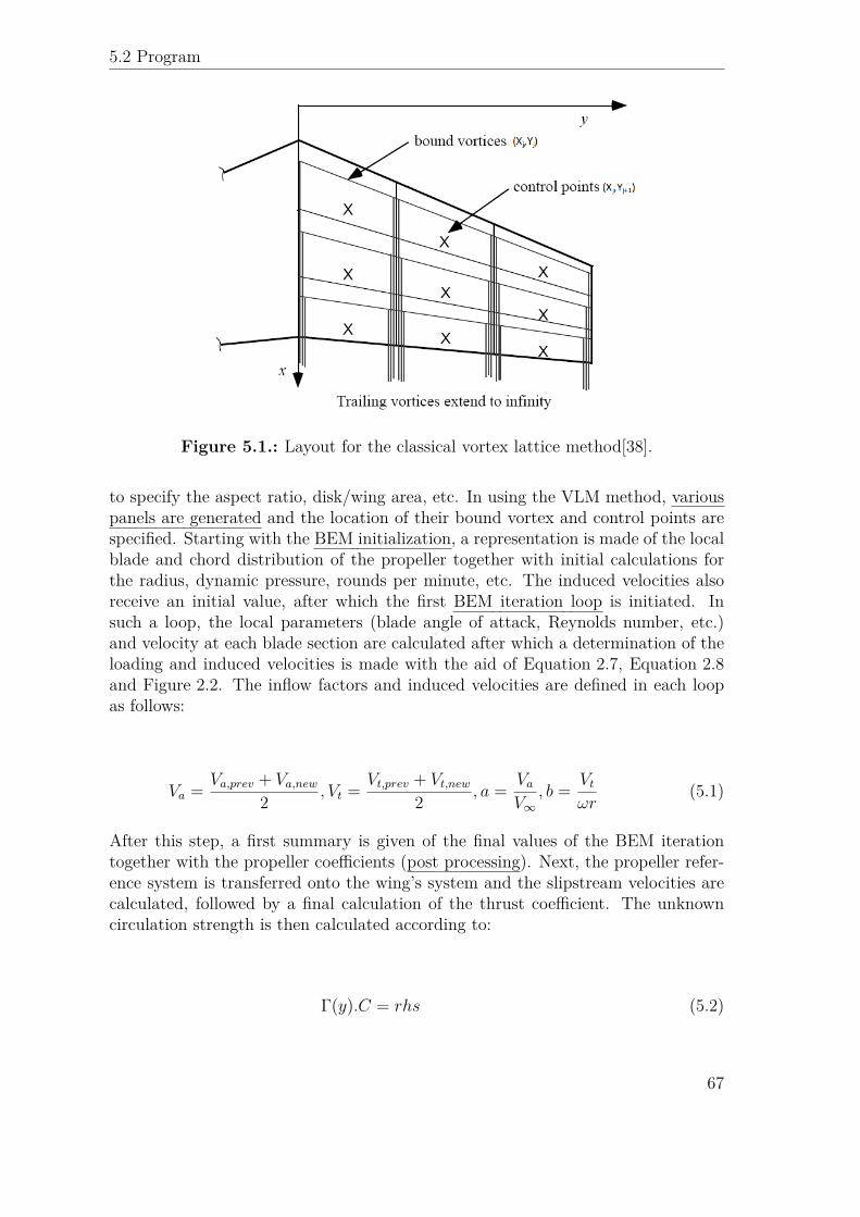
5.2 Program
Figure 5.1.: Layout for the classical vortex lattice method[38].
to specify the aspect ratio, disk/wing area, etc. In using the VLM method, variouspanels are generated and the location of their bound vortex and control points arespecified. Starting with the BEM initialization, a representation is made of the localblade and chord distribution of the propeller together with initial calculations forthe radius, dynamic pressure, rounds per minute, etc. The induced velocities alsoreceive an initial value, after which the first BEM iteration loop is initiated. Insuch a loop, the local parameters (blade angle of attack, Reynolds number, etc.)and velocity at each blade section are calculated after which a determination of theloading and induced velocities is made with the aid of Equation 2.7, Equation 2.8and Figure 2.2. The inflow factors and induced velocities are defined in each loopas follows:
Va = Va,prev + Va,new2 , Vt = Vt,prev + Vt,new
2 , a = VaV∞
, b = Vtωr
(5.1)
After this step, a first summary is given of the final values of the BEM iterationtogether with the propeller coefficients (post processing). Next, the propeller refer-ence system is transferred onto the wing’s system and the slipstream velocities arecalculated, followed by a final calculation of the thrust coefficient. The unknowncirculation strength is then calculated according to:
Γ(y).C = rhs (5.2)
67

Chapter 5 Interference effects of installed propeller
where rhs is the right hand side, which contains the velocity components over thewing as affected by the propeller slipstream and matrix C holds the influence of thehorse shoe vortex on the velocity in each control point.
A representation is made of the lift and loading distribution together with a shortsummary that includes the wing’s lift, drag, rolling moment and propeller coeffi-cients. The lift distribution is given with the aid of the following formula:
Cl(y) = 2Γ(y)V∞c(y) (5.3)
Important to note is that until now only the influence of the propeller on the wingis taken into account and not yet the secondary influence, i.e. the wing influenceon the propeller. Based on the calculated Γ - distribution, the incoming flow fieldfor the propeller is redefined. With the final induced velocities for the propeller, theBEM calculations are repeated. This is done for both propellers separately as theinduced velocities for the left and right side can be different due to the asymmetryin the loading distribution. Afterward, the same sequence is followed as before,i.e. the transfer of the propeller onto the wing’s system and the calculation of thecirculation distribution. At the end, a final summary with full interaction is given.A full overview and understanding can be found in [27] and a flow diagram is givenin Figure 5.2.
5.3. Investigation
Point of focus
The part of the wing that is immersed in the slipstream will notice a variation in α.By changing the Reynolds number or taking the cases of experiment and full scale,the fluctuations in the angle of attack in the immersed part of the wing will alteragain. As already mentioned, it is not of great importance in our case what theseexact values are, but more how the variation in local angle of attack of the wing isaltered in accordance to the error between full scale and experiment, i.e. the changein the angle of attack variation(4(4α)). A direct effect due to this change and as aconsequence of the Reynolds variation is the change in loading distribution over thewingspan. By using the different polars, characterizing the difference between fullscale and experiment, an analysis can be made with different loading distributionsas result. As is it is very difficult to map 4(4α), it is more convenient to put thefocus on the final loading (lift) distribution that results at the end of the VLM4Dprogram.
68

5.3 Investigation
Figure 5.2.: Flow diagram for the analysis part of VLM4D.
69

Chapter 5 Interference effects of installed propeller
5.3.1. Implementation of the propellers
For this investigation, we use the propellers from [12], since they were also used inour previous analysis. For most of the parameters in the input box of the VLM4Dprogram, it is argued that general values will be used. For example we do not useany sweep and the effect of the fuselage and nacelle is left out. Several adaptationsto this general lay out will be made further on in the report. Also the propeller angleand nacelle angle w.r.t. their reference axis are zero. The most important input thatwill influence our investigation is the airfoil data of the propeller that, as alreadymentioned, characterizes the full scale and experiment. In doing so, we can see howthe difference in performance of the propeller is translated into the slipstream andonto the wing loading distribution. So in practice, the propeller geometry togetherwith the different propeller polar data is of primary importance and the polars ofthe wing only of secondary importance. It is important to note that by using thedifferent propeller polar data, defined as in section 4.2.1., a representation is madefor the WT and FS case. Again, the main interest is to see the overall effect intothe loading distribution and not necessarily the specific values.
As expected, it can be seen in Figure 5.3 that the lift coefficient takes more extremevalues at local points of minimum and maximum in the rotor disk area. An overviewof the differences between WT and FS is given in Figure 5.4. The lift distributionsfor WT and FS for the other propellers are given in Appendix E.
�
���
���
���
���
���
���
��
� ��� ��� ��� ��� � ��� ��� ��� ��� �
��
�������
�
��
Figure 5.3.: Local lift coefficient in spanwise direction for WT and FS case ofpropeller L, J = 0.511 and the general wing lay out (in mm). [12]
70

5.3 Investigation
�����
����
�����
�
����
���
����
���
�� ���� ���� ��� ���� � ��� �� ��� ��� �
�����
�
�������
Propeller 4CL
CLW T
B 0.0658I 0.0707D 0.0853K 0.082L 0.0705
Figure 5.4.: The local difference in CL between WT and FS w.r.t. the wing’slift coefficient for propeller L (left), together with an overview for all propellers(right). [12]
5.3.1.1. Influence of Reynolds number augmentation on the lift (distribution)
For the propellers of [12], a clear difference is noticed between WT and FS. It shouldbe noted that the difference between experiment and full scale due to Re is consis-tent. To see the effect of a wide range of Reynolds numbers on the lift distribution,another analysis can be made with data from [9]. Here, typical polars for differentReynolds numbers are given for both wings and propellers. As a simple example, thepolars from Figure 1.5 can be used. The exact values of the lift distribution are ofsecondary importance, as we are merely interested in the change of the distributionwith the Reynolds number. The results are shown in Figure 5.5, and a close-up ismade in Figure 5.6.
It can be seen that the improvement becomes smaller when we reach Re values forfull scale. The difference between case 1 and 2 is responsible for the larger partof the entire difference. This is in agreement with the theory, where it was statedthat above values of Rec > 7×10⁵, the corrections become small for models [44]. InTable 5.1, some interesting parameters are given for Figure 5.5.
An important value in this table is the differences between Case 3 and Case 1, as∆Re is similar to the one from our previous investigation. It appears that the valuefor ∆CL
CLcase1in Table 5.1 is in agreement with the one found in Figure 5.3, where
∆CL
CLcase1= 0.0705.
71

Chapter 5 Interference effects of installed propeller
�
���
���
���
���
���
���
��
� ��� ��� ��� ��� � ��� ��� ��� ��� �
��
�������
� ����
� ����
� ����
� ����
RecCase 1 3.3×10⁵
Case 2 6.7×10⁵
Case 3 1.3×10⁶
Case 4 3.1×10⁶
Figure 5.5.: Influence of Re on the lift distribution with propeller section fromFigure 1.5, J = 0.45, on the same wing as in Figure 5.3.
����
���
����
���
����
��� ���� ��� ���� ��� ����
��
�������
���
����
����
����
Figure 5.6.: Influence of Re on the lift distribution with propeller section fromFigure 1.4, zoomed in for values of 0.2 < y
b/2 < 0.45.
Case 1 Case 2 Case 3 Case 4∆CL
CLcase1/ 0.053 0.072 0.083
(∆Cl)max,1CLcase1
/ -0.051 -0.077 -0.094(∆Cl)max,1CLcase1
/ 0.116 0.166 0.194Table 5.1.: Overview of differences in lift distribution affected by Re, w.r.t case 1.
72

5.3 Investigation
5.3.1.2. Influence of other parameters on Re-effect in the lift distribution
Propeller position
In [17], it was proven that by moving the propeller towards the tip, an increase inwing efficiency is noticed. Here, an investigation is done in order to see how the liftdistribution will change with a shift in the propeller’s position. The propellers from[12] are analyzed, where the propeller is shifted from | y
b/2 |= 0.5 to the position| yb/2 |= 0.6. Figure 5.7 shows the results before and after the shift.
An outward shift of the lift distribution was expected, but it can also be seen thatthe local lift coefficients are lower at the outboard side of the propeller. On theother hand, a larger part of the wing is now characterized by a higher lift coefficient.This means that the wing’s lift coefficient is also higher. It appears that the increasefor WT remains smaller than the one for FS. This would imply that the differencebetween WT and FS is aggravated as the propeller is shifted towards the tip. Inother words, the difference in lift coefficient due to Re, i.e. ((4CL)Re), will increasewhen the propeller is shifted outboard, as seen Figure 5.7.
�
���
���
���
���
���
���
��
� ��� ��� ��� ��� � ��� ��� ��� ��� �
��
�������
� �����������
�������������
�
��
yb/2 (4CL)Re0.5 0.070.6 0.088
Figure 5.7.: Comparison of the lift distribution for WT and FS, with and withouta shift towards the tip for propeller L, J = 0.511. [12]
If we do the same analysis for Figure 5.5, we see the same trend as for our previouspropellers. A good way of comparing the data, is to look at Table 5.2. It appearsthat, although the same trend is visible, the differences become larger in case of apropeller that is positioned more outboard.
73

Chapter 5 Interference effects of installed propeller
Before shift Case 1 Case 2 Case 3 Case 4∆CL
CLcase1/ 0.053 0.072 0.083
After shift∆CL
CLcase1/ 0.056 0.077 0.089
Table 5.2.: Changes in lift distribution as affected by Re, w.r.t case 1.
Wing planform
In the previous part, the effect of λ was left out. Here, an adaptation is made tothe wing planform by altering λ. In Figure 5.8 some visible changes can be noticedwhen the taper is decreased from a value of 1.0 to 0.7. Equation 5.3 states thatthe lift coefficient is proportional to 1
c, which means that higher values of the lift
coefficient are seen towards the outboard part of the wing.
�
���
���
���
���
���
���
��
� ��� ��� ��� ��� � ��� ��� ��� ��� �
��
�������
� ������������
��������������
�
��
λ (4CL)Re1 0.07050.7 0.0749
Figure 5.8.: Comparison of the lift distribution for WT and FS, with different λfor propeller L, J = 0.511.
Propeller diameter
In this last section, we will try to investigate to what extent (4CL)Re is affected bythe propeller diameter. As an example, the propeller of the previous section will betaken and the radius is decreased with 30 %. It can be seen in Figure 5.9 that bydecreasing the radius of the propeller, the overall lift becomes smaller but that also(4CL)Re decreases.If we now evaluate the adaptations of all the previous parameters, a general trendcan be seen. When and adaptation is made that leads to an augmentation of the
74

5.4 Intermediate conclusion installed propeller
�
���
���
���
���
���
���
��
� ��� ��� ��� ��� � ��� ��� ��� ��� �
��
�������
� ��������������
����������������
�
��
D (%) (4CL)Re100 0.070570 0.06750 0.045
Figure 5.9.: Comparison of the lift distribution for WT and FS, with a decreasein radius for propeller L, J = 0.511.
wing’s lift distribution, an increase of (4CL)Re is noticed. This also implies that theeffect of Re diminishes when the adaptation leads to a decrease in lift distribution.
5.4. Intermediate conclusion installed propeller
The intention in this chapter was to visualize how the difference in propeller datawould influence other points of interest like the wing. A straightforward and clearway to do this was by looking at the lift distribution of the wing and see howthis distribution would be affected by the propeller. At first, a description wasgiven of the general effects that induced velocities of propellers have on a wing.The interference program was used in order to see if the adaptation, characterizingthe effect of the Reynolds number, would also reveal the same general image asmentioned previously. By looking at the different propellers of [12], a similar trendwas noticed: more extreme values were noticed for higher Re. It appeared that theincrease in local lift coefficient on the upgoing blade was larger than the decreaseof the downgoing blade. The final result of this observation was an increase in thewing’s lift coefficient for higher Re. In a second stage, an analysis was made to seethe effect of a certain Re increase on the lift distribution. The improvement on thelift distribution became smaller as we reached higher Re values. In the previouschapter, a difference of around 8 %, was seen in the propeller performance data asconcluded. This chapter showed that this difference resulted in an error of over 7%on average at the wing when we focused on the loading distribution.
75

Chapter 5 Interference effects of installed propeller
Hereafter, another investigation was made to see how the lift distribution changeswith a certain Re. In order to do this, different polars were used that are character-ized by certain Re. It was seen that the biggest part of the improvement of the liftdistribution was situated in the lower region of Re (< 7×10⁵). We also noticed thatthe lift increase for the propellers from [12] was similar to the increase of the corre-sponding4Re in Figure 5.5. As a final analysis, we looked at the effect of parameterchanges on the Re-effect in the lift distribution (propeller position, diameter, wingtaper). For an outboard shift of the propeller, we did not only find an outward shiftof the lift distribution, but also lower values of the lift coefficient on the side of thedowngoing blade. This eventually resulted in an increase of the Re-effect. For anincrease in propeller diameter or a decrease in wing taper, an increase in Re-effectcould also be noticed. This led to the conclusion that for any previously mentionedadaptation, (4CL)Re became larger in case that the specific adaptation resulted ina lift augmentation over the wing.
76
6. Conclusions and recommendations
In preparation of this project and also during the research it was very importantto keep track of the objective and research questions. By concentrating on thescaling effects and more in particular the Re number effects, we needed a thoroughunderstanding on how this parameter could influence the major characteristics likelift, drag, etc. It was noticed that in general for an increase of Re, an augmentationof the maximum lift coefficient and its linear slope was observed together with adecrease of the drag coefficient. With this knowledge, it was clear how the effectof the Reynolds number could be implemented into the calculations that were donewith different programs.Before the investigation was started, it was necessary to investigate which programwas most compatible for a representation of our point of interest. In order to do this,several papers were used and presented in different programs. As a result, Qpropearned our preference in this case.Another important aspect was the limitation of the Reynolds number. In earlierstudies it was well argued that above values of 3×10⁵, representable data could befound for the full scale and that for this reason investigations were performed withthe crude rule of using Re > 5×10⁵. It was also mentioned that under values of2×105 no reliable data could be gathered in general as below this value unwanted andunexpected deviations appeared. In this work papers were used of values > 3×10⁵.By taking this lower limit, it is clear that the resemblance between full scale andwind tunnel only gets better with increasing Reynolds number and that the effectof scaling is at its highest value here. This statement holds as for lower valuesno reliable representation can be made. As a result no conclusions can be drawnunder this region. From different papers that laid their focus on scaling effects,different formula were stated that mainly focused on the improvement of the liftpolar. In this project, the focus is then merely centralized around this improvement.Although enough reasons are present to neglect the adaptation of the drag, it couldbe recommended to incorporate the influence of Re on drag when using the differentprograms. This recommendation can be implemented in two ways: one could analyzewhich input data in the program is available for adaptation in order to include theinfluences or one could adapt the program in case the deviations in the area ofinterest are not yet incorporated.As the limitations and effects were clear, the investigation was started in the nextpart by analyzing the different propellers. This was done by using the data that char-acterizes the deviation between wind tunnel and full scale tests. In a first instance
77

Chapter 6 Conclusions and recommendations
the focus was put on the uninstalled propeller, i.e. the performance characteris-tics. With the aid of known performance data, we were able to make an analysisin Qprop and see how well the reference data could be represented. As a result,good agreement was found for the slope of the performance data between tests andprogram. This resemblance was mainly manifested in larger values of the advanceratio. Despite this resemblance, there was still room for improvement between theused data. The reason for this deviation could be found in the lack of consistencybetween the data. Despite this observation, it was seen that the general conclusionsfrom the paper [12] hold, as the difference due to the scaling effect in the programwas in agreement with the one found in tests.The question about consistency of some used data needs further clarification. Thiswas done in section 4.2, where it was pointed out that the unwanted deviation ofdata in the program is most certainly emanating from an incorrect use of availabledata points since in our case it was noticed that different values for one particularcase were found. For this reason, it is recommended that the investigation should besupported by taking other data from airfoils in order to get a perfect match betweenthe results from the program and paper.Other important results that were investigated are the differences in induced veloc-ities, which followed directly from the differences in the performance data. Also inthis stage the scaling effect could be seen.An interesting question that came up while doing the investigation was whether ornot the choice of constant advance ratio for the propeller performance was the bestone. In order to give a good answer, the different variables (thrust coefficient andadvance ratio in our case) were held constant separately. As a good match wassought, we focused on how the induced velocities would behave for propellers in WTand FS tests.Focusing on the different induced velocities, it appeared rather quick that the use ofconstant thrust coefficient gave an overshoot in comparison with FS. For constantJ , the differences in both axial and swirl velocities were smaller compared to thedifferences found when CT was kept constant. An exception was found for theouter part ( r
R> 0.7) of the radius at constant CT , where the difference in swirl
velocity became smaller than for a constant J . As a conclusion, the specific valuesfor constant J are given:
• In case of constant J , an increase of 0.3 % towards the root and 0.8 % atthe tip was found on average, with a maximum of 1% at r
R= 0.75. For the
tangential velocities, an increase of 0.2% is seen towards the tip which increasesto a value >0.3% in the direction of the root. This difference remained ratherconstant along the radial position, unlike the difference in case of the axialvelocities. These differences have a direct implication on the local inflow angle:an increase was seen of 3% at r
R= 0.2 and 5% towards the tip.
It can also be seen that the Reynolds effect in the propeller performance re-sults in a ’chain reaction’, i.e. 4CT = 4Va,4CQ = 4Vt and 4(4α) in the
78

Conclusions and recommendations
slipstream. By using an interaction program in the last chapter, we saw thatthe scaling effect on the propeller also affects the wing. The ’4(4α)’, or infull words the fluctuation caused by scaling effect on the fluctuation of theangle of attack as a consequence of the slipstream, could be an interesting pa-rameter to keep track of. A method of looking into the effect of 4(4α), wasby investigating how the wing’s lift distribution is altered, as a consequence ofthe data of the uninstalled propeller.In investigating the different propellers, the same trends as from theory wherenoticed in the program. More in particular, these trends contain the differencesbetween quasi elliptical loading distributions and loading distributions in thepresence of a propeller. The difference between the full scale and wind tunneldata could especially be seen at positions where the blade tip crossed the wing.The final result of this analysis resulted in a deviation of over 7% on averagefor the wing’s lift coefficient between WT and FS when a general wing lay outwas used.In order to see how the lift distribution changes with a certain Re increase,another investigation was conducted where different polars were used thatcharacterize certain Re. It was seen that the biggest part of the improvementof the lift distribution was situated in the lower region of Re (< 7×10⁵).Finally, we focused on the effect of parameter changes on the Re-effect in thelift distribution (propeller position, diameter, wing taper). This led to theconclusion that for any previously mentioned adaptation, (4CL)Re becamelarger in case that the specific adaptation resulted in lift augmentation overthe wing.
79


Acknowledgments
As I am almost at the point of receiving the degree in Master of Science, it is timeto show my gratitude to the following people as this was not possible without theirsupport and advice.First of all I would like to thank Mr. Veldhuis for his guidance and feedback through-out the entire project. In addition I would like to express my appreciation to Mr.Eitelberg and Mr. Timmer for taking part in my Graduation committee.I am also thankful to my fellow graduates for making my working place a pleasantand productive environment. My friends outside the faculty also earn my gratitudeas they kept my mind and spirit fresh by taking breaks outside the university fromtime to time.An Claes, Herman Ghekiere and Jens Vande Cavey also deserve my gratitude, read-ing my report in order to find flaws and imperfections.And most important I would like to thank my family, especially my mother, for herpersistent support and constant pushing, together with the support they gave meduring difficult times.
81


Bibliography
[1] http://www.mh-aerotools.de/airfoils/javaprop.htm
[1b] Adkins, C. N.: Design of Optimum Propellers, AIAA-83-0190. Also publishedin the Journal of Propulsion and Power, Vol. 10, No. 5, September-October1994.
[2] http://www.drivecalc.de/PropCalc/PCHelp/Help.html
[3] Edwin P. Hartman and David Biermann, “The aerodynamic characteristics offull-scale propellers having 2,3 and 4 blades of Clark Y and R.A.F.-6 airfoilsections”, NACA report 640.
[4] Hugh B. Freeman, “Comparison of full-scale propellers having R.A.F.-6 andClark Y airfoil sections”, NACA report 378.
[5] Blake W. Corson and Julian D. Maynard, “Investigation of the effect of tipmodification and thermal de-icing airflow on propeller performance”, NACATN 1111.
[6] George W. Stickle and John L. Crigler, “Propeller analysis from experimentaldata”, NACA report 712
[7] http://web.mit.edu/drela/Public/web/qprop/qprop_doc.txt
[8] M. Dimchev, “Experimental and numerical study on wingtip mounted pro-pellers for low aspect ratio UAV design”, Msc thesis report, Delft University ofTechnology, 2012.
[9] Eastman N. Jacobs and Albert Sherman, “Airfoil sections characteristics aseffected by variations of the Reynolds Number”, NACA-1937.
[10] S. Breton, “Study of the stall delay phenomenon and of wind turbine blade aero-dynamics using numerical approaches and NREL’s wind tunnel tests”, Doctoralthesis, Norwegian University of Science and Technology, Trondheim, 2008.
[11] H.snel, R. Houwink, J. Bosschers, “Sectional prediction of lift coefficients onrotating wind turbine blades in stall”, ECN, ECN-C–93-052, May 1993
[12] W. F. Durand and E. P. Lesley, “Comparison of tests on air propellers in flightwith wind tunnel model tests on similar forms.” NACA TN220
[13] W. S. Diehl, “The variation of aerofoil lift and drag coefficients with changesin size and speed.” NACA TN 111, 1921
83

Bibliography
[14] P. Giguere and M. S. Selig, “Low Reynolds number airfoils for small horizontalwind turbines.” University of Illinois.
[15] Christopher A. Lyon, Andy P. Broeren etc.,”Summary of low-speed airfoildata.” Vol. 1, SoarTech Publications, Virginia Beach, VA, 1995, 292 pages.
[16] Abe Silverstein, “Scale effect on Clark Y airfoil characteristics from NACAfull-scale wind-tunnel tests.”, NACA report 502.
[17] R. Miranda and E. Brennan, “Aerodynamic effects of wingtip-mounted pro-pellers and turbines.” AIAA-1986-1802.
[18] P. B. S. Lissaman, “Low-Reynolds-number airfoils”, Ann. Rev. Fluid Mech.1983, 15: 223-39, California.
[19] D. F. Volkers, “Preliminary results of wind tunnel measurements on some airfoilsections at Reynolds numbers between 0.6 x 10⁵ and 5.0 x 10⁵”,Delft Universityof Technology, 1977.
[20] Richard Eppler and M. Somers, “Airfoil design for Reynolds numbers between50000 and 500000”, Conference on low Reynolds number airfoil aerodynamics,page nr. 1, June 1985.
[21] J. Miley, M. Howard and J. Holmes,”Wing laminar boundary layer in the pres-ence of a propeller slipstream.” Journal of Aircraft, Vol. 25, No. 7 (1988).
[22] M. George and E. Kisielowski, “Investigation of propeller slipstream effects onthe wing performance”, (Book) 1st edition published in 1967.
[23] L. Veldhuis, “Propeller Wing Aerodynamic Interference.” Phd thesis, Delft Uni-versity of Technology, 2005.
[24] Dave P. Witkowksi, Alex K. H. Lee and John P. Sullivan, “Aerodynamic inter-action between propellers and wings”, Purdue University, VS, AIAA-1988-0665.
[25] Bertin, J.J., and Smith, M.L., Aerodynamics for Engineers, Prentice-Hall, Inc.,Englewood Cliffs, 2nd Ed., 1989, pp: 261-282, 3rd Ed. 1998, pp: 291-311.
[26] W.H.Mason, “Applied Computational Aerodynamics Text/Notes.” ( Vol1,Chapter 6; http://www.dept.aoe.vt.edu/~mason/Mason_f/CAtxtTop.html)
[27] L. Veldhuis, “Vortex Lattice Analysis of a Twin-engine Tractor Propeller-WingModel.” Mathcad program: -VLM4D-
[28] B. W. McCormick. Aerodynamics, aeronautics and flight mechanics. John Wi-ley and Sons, Inc., second edition edition, 1995. ISBN 0-471-57506-2.
[29] L. Veldhuis and S. Nebiolo, “A propeller-integration study comparing exper-imental data with numerical flow solutions based on the navier-stokes equa-tions”, Harrogate, UK, ICAS congress 2000, paper 264.
[30] M. A. Takallu and G. L. Gentry Jr., “ Aerodynamic characteristics of a propellerpowered high lift semi-span wing”, Virginia, US, AIAA-1992-388.
84

Acknowledgments
[31] P. C. M. van den Borne and J. van Hengst, “Investigation of propeller slip-stream effects on the Fokker 50 through in-flight pressure measurements”, theNetherlands, AIAA-1990-3084.
[32] M. Lino, ”Numerical investigation of propeller-wing interaction effects for alarge military transport aircraft.”, Thesis report, Delft University of Technology,2010.
[33] F. M. Catalano, “On the effects of an installed propeller slipstream on wingaerodynamic characteristics”, Acta Polytechnica Vol. 44 No. 3/2004.
[34] M Drela QPROP user guide, 2005.[35] M. K. Rwigema, “Propeller blade element momentum theory with vortex wake
deflection”, Proceedings of the 27th Congress of the International Council ofthe Aeronautical Sciences, Nice, France, September 19–24, 2010.
[36] M. Brenckmann, “Experimental investigation of the aerodynamics of a wing ina slipstream”, Toronto University, Journal of Aeronautics, 1957.
[37] S. J. Miley, R.M. Howard and B.J. Holmes, “Propeller Slipstream/Wing bound-ary layer effects at low Reynolds numbers”, Conference on low Reynolds numberairfoil aerodynamics, page nr. 335, June 1985.(page 342 for figure Figure 4.3)
[38] R. Enoiu, “Application of vortex lattice method to analyze the performance ofa glider”, Fascicle of Management and Technological Engineering, Volume VI(XVI), 2007.
[39] Hermann Schlichting, “Boundary Layer Theory”,page 695. ISBN 0-07-055334-3.[40] T. De Leeuw, “Investigation of scaling effects in propeller testing”, Delft, 2012[41] M. Lino,”Numerical investigation of propeller-wing interaction effects for a large
military transport aircraft”,Delft, 2010[42] Fred E. Weick, “Propeller scale effect and body interference”, Bureau of Aero-
nautics, NACA-TC-225.[43] C. Rohrbach and F. B. Metzger, “The prop-fan, a new look in propulsors”,
Windsor Lock Connecticut, AIAA-1975-1208.[44] SAE-AIR-4065, page nr. 75.[45] L. Troost, “Reynolds number for model propeller experiments”, Report of In-
ternational Committee and Introductory, London conference, 1948.[46] H. E. Saunders, “The choice of suitable Reynolds number for model propeller
experiments”, Berlin conference 1937.[47] Antonio Filippone, “Data and performances of selected aircraft and rotorcraft”,
Progress in Aerospace Sciences 36 629-654, Denmark 2000.[48] Richard Eppler and Martin Hepperle, “A procedure for propeller design by in-
verse methods”, Stuttgart, Germany.( http://www.mh-aerotools.de/company/paper_1/epplerhepperle.htm last visited on 26 dec. 2011)
85

Bibliography
[49] John Stack, Eugene C. Draley James B. Delano and Lewis Feldman, “Investi-gation of the NACA 4-(3)(08)-03 and NACA 4-(3)(08)-45 two-blade propellersat forward mach numbers of 0.725 to determine the effects of compressibilityand solidity on performance”, NACA-Report 999.
[50] “Experiments on airfoil at low Reynolds numbers”, 34th Aerospace SciencesMeeting and Exhibit, AIAA-1996-62.
[51] V. Ustinov and P. Ostroukhov, “Experimental investigation of propellers atlow Reynolds numbers”, Competition, Workshop and Conference”, Toulouse,France, September 2007.
[52] R. M. Bass and D. G. M., “A review of some recent U.K. propeller develop-ments”, Gloucester, England, AIAA-1985-1261.
[53] McGraw-Hill series in mechanical engineering, Boundary Layer theory p. 694.[54] R. A. Wahls, L. R. Owens and S. M. B. Rivers,” Reynolds number effects on a
supersonic transport at transonic conditions”, Nevada, US, AIAA-2001-912.[55] Ehab A. Elsaadawy and Colin P. Britcher, “Experimental investigation of the
effect of propeller slipstream on boundary layer behavior at low Reynolds num-ber”, Old Dominion University, VS, AIAA-2000-4123.
[56] R.M. Howard, “An investigation of the effects of the propeller slip-stream on a wing boundary layer”, Texas, 1987. (http://adsabs.harvard.edu/abs/1987PhDT........47H : last visited on 22-12-2011)
[57] S. Goldstein, “On the vortex theory of screw propellers.”, Proceedings of theRoyal Society, 123, 1929.
[58] M. Arschwanden, “Wind tunnel simulation of propeller effects in the A400MFLA-4 model”, AIAA-2005-3706.
[59] W. Shyy,Y. Lian, “Aerodynamics for low Reynolds number flyers”, Cambridge,2008, ISBN 9780521882781.
[60] L. Veldhuis, “Review of propeller-wing aerodynamic interference”, ICAS 2004-6.3.1., 24th International Congress of the Aeronautical Sciences,Yokohama,Japan .
[61] C.Lindenburg, ”Investigation into rotor blade aerodynamics”, ECN-C–03-025,2003.
[62] http://web.mit.edu/drela/Public/web/qprop/qprop_theory.pdf
86

A. Validation of Mach and Reynoldsregimes
In section 1.3, we pointed out the general tip Mach en Reynolds regimes. A verifi-cation for these regimes was made at the end of that section for 2 different cases;the A400M and the F-50. The tables and calculations to validate the regimes arelisted below.
case 1: A400M
Table A.1Full scale (0 ft) Full scale (24000 ft) WT (1:15)
RecC3/4VRe
ν5× 10⁶ 9.2×10⁶ 4.8× 10⁵
MtVM
a0.68 0.78 0.61
J VnD
2.1 (low speed) 2.7 (high speed) 1with:VM(km/h) = RPM × Diameter × π × 60
1000
VRe= 2×π×r×RPM60
values for full scale:
C3/4= 0.45 m at 75% of chordDiameter= 5.3 mRPM= 864 (max)ν = 14.81.10-6 m2/s (at 293K and 0ft)ν = 9.01.10-6 m2/s (at 235K and 24000ft)true airspeed = 160 m/s (low)true airspeed = 210 m/s (high)a = 1255 km/h (0ft)a = 1093 km/h (24000ft)
87

Appendix A Validation of Mach and Reynolds regimes
values forWT (1:15):
C3/4= 0.03 mDiameter= 0.355 mRPM= 12000 mWT speed = 70 m/s
case 2: F-50
Table A.2Full scale (0 ft) WT (1:15)
RecC3/4VRe
ν3.5x× 106 4.8× 10⁵
MtVM
a0.68 0.45
J VnD
2.4 2.4
values for full scale:
C3/4= 0.3 mDiameter= 3.66 mRPM= 1200 (max)ν = 14.81.10-6 m2/s (at 293K and 0ft)true airspeed = 147 m/s
values forWT (1:15):
C3/4= 0.06 mDiameter= 0.7 mRPM= 4300WT speed = 100 m/s
88

B. Data preliminary survey
Different reports were used in section 3.3 to validate the accuracy of the theoreticalprograms. The data points, characterizing the performance of the propellers, arelisted below. Their corresponding graphs were already given in chapter 3.
Report 640
Report 640 Qprop PropCalcJ CT J CT J CT0.4 0.164 0 0.12 0.05 0.1320.5 0.162 0.1226 0.123 0.18 0.1330.6 0.159 0.2459 0.126 0.31 0.1350.7 0.156 0.368 0.13 0.44 0.13810.8 0.155 0.4919 0.134 0.57 0.14220.9 0.153 0.614 0.1398 0.63 0.14461.0 0.147 0.737 0.145 0.7 0.14721.1 0.134 0.86 0.15 0.83 0.15251.2 0.118 0.983 0.148 0.96 0.15381.3 0.1 1.1 0.139 1.02 0.15151.4 0.08 1.22 0.122 1.15 0.13991.5 0.062 1.35 0.099 1.28 0.1211.6 0.045 1.47 0.074 1.41 0.0991.7 0.025 1.59 0.05 1.54 0.07571.84 0.005 1.72 0.029 1.67 0.0522
1.84 0.004 1.8 0.03121.93 0.0123
89

Appendix B Data preliminary survey
Report 378
Report 378 Qprop PropCalcJ CT J CT J CT
0.15 0.0949 0 0.0855 0.05 0.08490.2 0.0861 0.0741 0.0860 0.12 0.08510.25 0.0826 0.148 0.0867 0.18 0.08550.3 0.0793 0.2212 0.0875 0.25 0.08570.35 0.0763 0.2954 0.0883 0.31 0.08480.4 0.0739 0.3695 0.0838 0.38 0.08090.45 0.07 0.4437 0.0762 0.44 0.07470.5 0.0655 0.5178 0.0665 0.51 0.06730.55 0.0586 0.5920 0.0554 0.557 0.05940.6 0.0518 0.6649 0.0441 0.64 0.0510.65 0.045 0.7319 0.0328 0.7 0.04220.7 0.038 0.8132 0.0221 0.77 0.03360.75 0.0309 0.8874 0.0127 0.83 0.02510.8 0.0238 0.9616 0.0049 0.9 0.01690.85 0.0165 1.0357 0 0.96 0.010.9 0.0091 1.03 0.00390.95 0.00018 1.06 0.0015
TN 1111
TN 1111 Qprop PropCalcJ CT J CT J CT
0.832 0.093 0 0.0749 0.73 0.10270.863 0.089 0.065 0.0754 0.78 0.10180.891 0.085 0.129 0.0761 0.84 0.09910.931 0.081 0.195 0.769 0.89 0.09450.978 0.0745 0.259 0.0779 0.94 0.08871.03 0.067 0.325 0.0790 0.99 0.08241.08 0.057 0.389 0.080 1.05 0.0761.14 0.0491 0.454 0.0817 1.1 0.06911.2 0.0399 0.520 0.0832 1.2 0.05491.24 0.0338 0.650 0.0865 1.26 0.04751.29 0.026 0.779 0.0898 1.31 0.03981.35 0.017 0.975 0.0758 1.36 0.03141.39 0.0099 1.104 0.0569 1.41 0.02321.43 0.0038 1.234 0.0369 1.47 0.0161.455 0 1.364 0.016 1.52 0.0089
1.428 0.005 1.57 0.0033
90

report 712
report 712 Qprop PropCalcJ CT J CT J CT
0.094 0.1046 0 0.110 0.05 0.11850.1987 0.1045 0.137 0.112 0.16 0.11870.2926 0.1035 0.273 0.115 0.27 0.11850.3933 0.1014 0.410 0.120 0.38 0.11270.494 0.098 0.546 0.116 0.49 0.10560.591 0.094 0.683 0.102 0.6 0.09630.695 0.0899 0.819 0.088 0.71 0.08670.792 0.088 0.956 0.073 0.82 0.07660.893 0.085 1.09 0.057 0.93 0.06620.993 0.0767 1.22 0.041 1.03 0.05531.097 0.0647 1.36 0.025 1.14 0.0441.194 0.0516 1.50 0.009 1.25 0.03271.304 0.0366 1.36 0.02141.401 0.0225 1.42 0.01581.497 0.0051 1.47 0.0102
1.53 0.0047
91


C. Validation and evaluation ofpropellers
Propeller B was already used as an example in the report and in this appendix thedata for the other 4 propellers are listed below, i.e. D,I,K and L. The data focuseson the analysis with Qprop, which is done in Chapter 4.
Reynolds number range for reference propellers
Rec(C3/4VRe
ν) WT FS
Propeller B 3.3× 10⁵ 1.7× 10⁶
Propeller D 3.7× 10⁵ 1.5× 10⁶
Propeller I 4.1× 10⁵ 1.6× 10⁶
Propeller K 3.2× 10⁵ 1.3× 10⁶
Propeller L 4.8× 10⁵ 1.5× 10⁶
propeller D
����
����
����
����
���
����
��� ��� ��� ��� �
��
�
���� � ����
���� � ����
���� � ������� ���
��� ��� ����
��� ��� ����
Figure C.1.: First data set without the Himmelskamp effect for propeller D.
93

Appendix C Validation and evaluation of propellers
�
����
����
����
����
���
����
����
��� ��� ��� ��� �
��
�
��� �����
��� �����
��� ����������
�������� ���
�������� ���
Figure C.2.: Second data set with the Himmelskamp effect for propeller D.
propeller I
�
����
����
����
����
���
����
��� ��� ��� ��� �
��
�
���� � ����
���� � ����
���� � ������� ���
�� ��� ����
��� ��� ����
Figure C.3.: First data set without the Himmelskamp effect for propeller I.
94

�
����
����
����
����
���
����
��� ��� ��� ��� �
��
�
��� �����
��� �����
��� ����������
�������� ���
�������� ���
Figure C.4.: Second data set with the Himmelskamp effect for propeller I.
propeller K
�
����
����
����
����
���
��� ��� ��� ��� �
��
�
���� � ����
���� � ����
���� � ������� ���
��� ��� ����
��� ��� ����
Figure C.5.: First data set without the Himmelskamp effect for propeller K.
95

Appendix C Validation and evaluation of propellers
�
����
����
����
����
���
����
��� ��� ��� ��� �
��
�
��� �����
��� �����
��� ����������
�������� ���
�������� ���
Figure C.6.: Second data set with the Himmelskamp effect for propeller K.
propeller L
�
����
����
����
����
���
����
��� ��� ��� ��� �
��
�
���� � ����
���� � ����
���� � ������� ���
��� ��� ����
��� ��� ����
Figure C.7.: First data set without the Himmelskamp effect for propeller L.
96

�
����
����
����
����
���
����
����
��� ��� ��� ��� �
��
�
��� �����
��� �����
��� ������ ���
�������� ���
�������� ���
Figure C.8.: Second data set with the Himmelskamp effect for propeller L.
97


D. Comparison with constantperformance parameters
Propeller B was already used as an example in the report and in this appendix thedata for the other 4 propellers are listed below, i.e. D,I,K and L. The data focuseson the resulting induced velocities of the two analysis done with Qprop, where eitherJ or CT is kept constant.
propeller D
�
���
���
���
���
�
���
���� ��� ���� ���
���
����
�
���
���
���
���
�
���
��� ���� ��� ����
���
����
��
Figure D.1.: Local axial velocities versus the radial position for full scale and windtunnel of propeller D with constant advance ratio (left) and constant thrust coef-ficient (right).
99

Appendix D Comparison with constant performance parameters
�
����
����
����
����
����
����
���
���
����
���
� ��� ��� ��� �� �
����
���
�
��
�
����
����
����
����
����
����
���
���
����
���
� ��� ��� ��� �� �
����
���
�
��
Figure D.2.: Local tangential velocities versus the radial position for full scale andwind tunnel of propeller D with constant advance ratio (left) and constant thrustcoefficient (right).
�
���
�
���
�
���
�
���
�
���
�
� ��� ��� ��� �� �
�
���
�
�
Figure D.3.: Inflow angle in function of the radial position for WT and FS casefor propeller D.
100
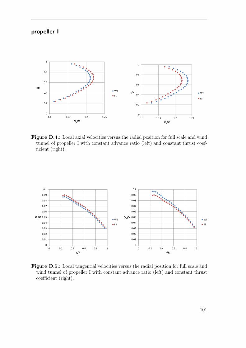
propeller I
�
���
���
���
���
�
��� ���� ��� ����
���
����
��
�
���
���
���
���
�
��� ���� ��� ����
���
����
��
Figure D.4.: Local axial velocities versus the radial position for full scale and windtunnel of propeller I with constant advance ratio (left) and constant thrust coef-ficient (right).
�
����
����
����
����
����
����
���
���
����
���
� ��� ��� ��� �� �
����
���
�
��
�
����
����
����
����
����
����
���
���
����
���
� ��� ��� ��� �� �
����
���
�
��
Figure D.5.: Local tangential velocities versus the radial position for full scale andwind tunnel of propeller I with constant advance ratio (left) and constant thrustcoefficient (right).
101
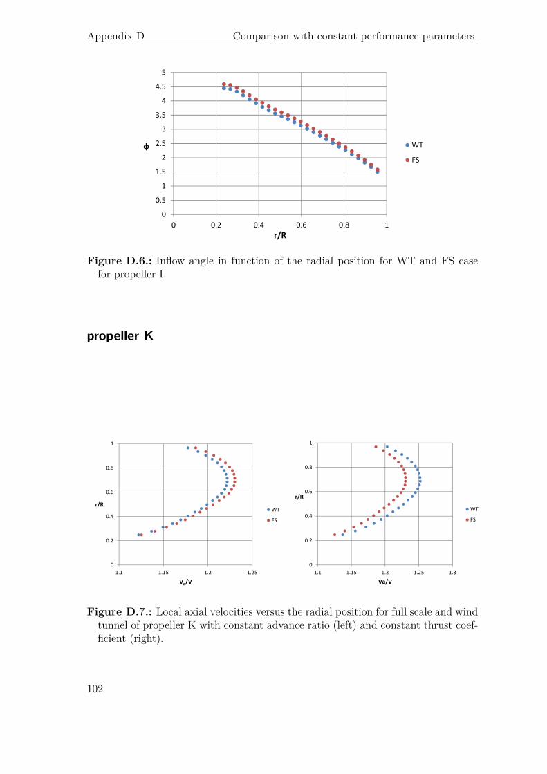
Appendix D Comparison with constant performance parameters
�
���
�
���
�
���
�
���
�
���
�
� ��� ��� ��� �� �
�
���
�
�
Figure D.6.: Inflow angle in function of the radial position for WT and FS casefor propeller I.
propeller K
�
���
���
���
���
�
��� ���� ��� ����
���
����
��
�
���
���
���
���
�
��� ���� ��� ���� ��
���
����
�
�
Figure D.7.: Local axial velocities versus the radial position for full scale and windtunnel of propeller K with constant advance ratio (left) and constant thrust coef-ficient (right).
102

�
����
����
����
����
����
����
���
���
����
���
� ��� ��� ��� �� �
����
���
�
��
�
����
����
����
����
����
����
���
���
����
���
� ��� ��� ��� �� �
����
���
�
��
Figure D.8.: Local tangential velocities versus the radial position for full scale andwind tunnel of propeller K with constant advance ratio (left) and constant thrustcoefficient (right).
Figure D.9.: Inflow angle in function of the radial position for WT and FS casefor propeller K.
103

Appendix D Comparison with constant performance parameters
propeller L
�
���
���
���
���
�
��� ���� ��� ����
���
����
��
�
���
���
���
���
�
��� ���� ��� ����
���
����
��
Figure D.10.: Local axial velocities versus the radial position for full scale andwind tunnel of propeller L with constant advance ratio (left) and constant thrustcoefficient (right).
�
����
����
����
����
����
����
���
���
����
���
� ��� ��� ��� �� �
����
���
�
��
�
����
����
����
����
����
����
���
���
����
���
� ��� ��� ��� �� �
����
���
�
��
Figure D.11.: Local tangential velocities versus the radial position for full scaleand wind tunnel of propeller L with constant advance ratio (left) and constantthrust coefficient (right).
104

Figure D.12.: Inflow angle in function of the radial position for WT and FS casefor propeller L.
Difference in induced velocities between WT and FS withconstant J
Prop
ellerB
Prop
ellerI
Prop
ellerD
r R4V
a
V∞
4V
t
V∞
4ϕ
ϕlo
ca
l
4V
a
V∞
4V
t
V∞
4ϕ
ϕlo
ca
l
4V
a
V∞
4V
t
V∞
4ϕ
ϕlo
ca
l
0.23
0.0039
0.0031
0.036
0.0029
0.0029
0.031
0.0028
0.0027
0.029
0.35
0.0061
0.0034
0.040
0.0054
0.0032
0.034
0.0044
0.0029
0.033
0.45
0.0079
0.0035
0.044
0.0063
0.0032
0.037
0.0056
0.0030
0.036
0.59
0.0100
0.0035
0.049
0.0084
0.00323
0.041
0.0072
0.0029
0.041
0.71
0.0109
0.0031
0.052
0.0092
0.0030
0.044
0.0084
0.00269
0.045
0.80
0.0109
0.0028
0.054
0.0096
0.0026
0.047
0.0084
0.00236
0.048
0.92
0.0100
0.0021
0.056
0.0084
0.0019
0.050
0.0076
0.00179
0.0052
0.96
0.0092
0.0019
0.058
0.0084
0.0018
0.052
0.0072
0.0016
0.053
Prop
ellerK
Prop
ellerL
r R4V
a
V∞
4V
t
V∞
4ϕ
ϕlo
ca
l
4V
a
V∞
4V
t
V∞
4ϕ
ϕlo
ca
l
0.23
0.0031
0.0026
0.027
0.0032
0.0032
0.034
0.35
0.0045
0.0028
0.029
0.0052
0.0035
0.037
0.45
0.0059
0.0029
0.033
0.0072
0.0036
0.040
0.59
0.0081
0.0029
0.036
0.0088
0.0036
0.044
0.71
0.0086
0.0027
0.040
0.0100
0.0032
0.047
0.80
0.0090
0.0024
0.042
0.0104
0.0029
0.050
0.92
0.0086
0.0019
0.045
0.0096
0.0022
0.053
0.96
0.0086
0.0017
0.046
0.0084
0.0019
0.054
105

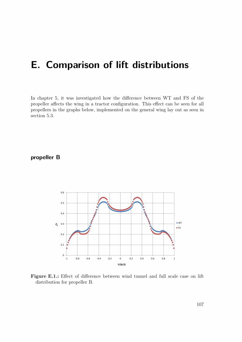
E. Comparison of lift distributions
In chapter 5, it was investigated how the difference between WT and FS of thepropeller affects the wing in a tractor configuration. This effect can be seen for allpropellers in the graphs below, implemented on the general wing lay out as seen insection 5.3.
propeller B
�
���
���
���
���
���
���
� �� ��� ��� ��� � ��� ��� ��� �� �
��
�������
��
�
Figure E.1.: Effect of difference between wind tunnel and full scale case on liftdistribution for propeller B.
107
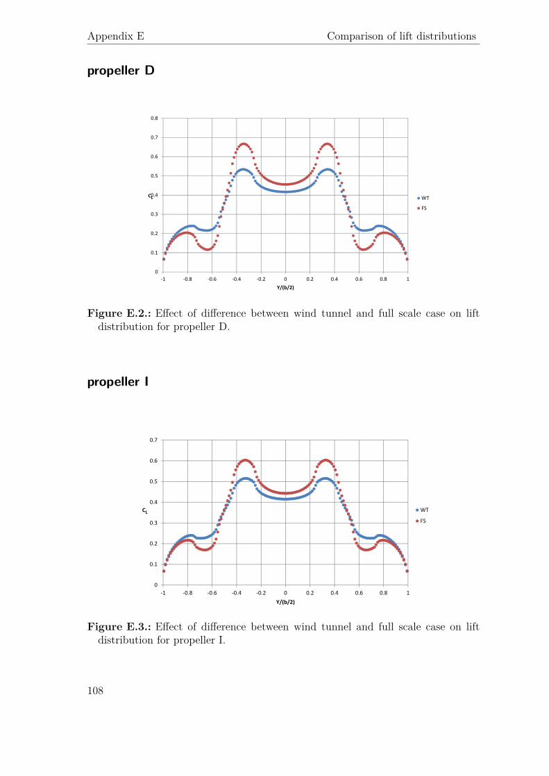
Appendix E Comparison of lift distributions
propeller D
�
���
���
���
���
���
���
��
��
�� ��� ���� ���� ���� � ��� ��� ��� �� �
��
�������
�
��
Figure E.2.: Effect of difference between wind tunnel and full scale case on liftdistribution for propeller D.
propeller I
�
���
���
���
���
���
���
��
� ��� ��� ��� ��� � ��� ��� ��� ��� �
��
�������
�
��
Figure E.3.: Effect of difference between wind tunnel and full scale case on liftdistribution for propeller I.
108

Propeller K
�
���
���
���
���
���
���
��
� ��� ��� ��� ��� � ��� ��� ��� ��� �
��
�������
�
��
Figure E.4.: Effect of difference between wind tunnel and full scale case on liftdistribution for propeller K.
109

![August 5th 2010 - NASA · PropCalc Several graphs with one point from each graph Final graph of thrust required . 0 5 10 15 20 25 30 35 40 45 50 0 20 40 60 80 [f] Velocity [knots]](https://img.dokumen.tips/doc/110x75/5ad3ba777f8b9a571e8b51a0/august-5th-2010-nasa-several-graphs-with-one-point-from-each-graph-final-graph.jpg)


