Embed Size (px)
Citation preview

I
University of Southern Queensland
Faculty of Engineering and Surveying
Investigation on utilising Real Time Kinematic (RTK) Global
Navigation Satellite Systems (GNSS) for Electronic Distance
Measurement (EDM) Baseline Calibration and Traceability of
Measurement.
A Dissertation submitted by
Mr Michael James Bissett
In fulfilment of the requirements of
COURSE ENG4111 and ENG4112 Research Project
Towards the degree of
Bachelor of Spatial Science (Surveying)
Submitted: 28th October, 2008

II
ABSTRACT
As technological advances in equipment as applied to field surveying
measurement and data storage/recording continues to accelerate towards
previously unforeseeable limits, there still remains the onus to verify Electronic
Distance Measurement (EDM) equipment to a national standard and the
respective regulations that require a Surveyor to establish and maintain legal
traceability of measurement. Given the current trend of utilising Global
Navigation Satellite Systems (GNSS) for surveying applications, Electronic
Distance Measurement, which was once the benchmark of measurement devices
is being gradually replaced by GNSS systems. Notwithstanding, the lack of
suitable calibration baselines standardised in accordance with the National
Measurement Regulations for the purpose of EDM verification, appears to be
disappearing at an alarming rate. Many previous certified EDM baselines are in
a state of disrepair or they simply are no longer being certified on an ongoing
basis. This paper intends to deal with this problem of diminishing EDM
calibration baselines and look to an alternative method whereby utilising RTK
GNSS technology to provide a solution to the traceability and verification of
measurement of EDM devices back to a recognised standard.
III
University of Southern Queensland
Faculty of Engineering and Surveying
ENG4111 & ENG4112 Research Project
Limitations of Use
The Council of the University of Southern Queensland, its Faculty of Engineering and Surveying, and the staff of the University of Southern Queensland, do not accept any responsibility for the truth, accuracy or completeness of material contained within or associated with this dissertation. Persons using all or part of this material do so at their own risk, and not at the risk of the Council of the University of Southern Queensland, its Faculty of Engineering and Surveying or the staff of the University of Southern Queensland. This dissertation reports an educational exercise and has no purpose or validity beyond this exercise. The sole purpose of the course pair entitled “Research Project” is to contribute to the overall education within the student’s chosen degree program. This document, the associated hardware, software, drawings, and other material set out in the associated appendices should not be used for any other purpose: if they are so used, it is entirely at the risk of the user. Prof Frank Bullen Dean Faculty of Engineering and Surveying

IV
Certification
I certify that the ideas, designs and experimental work, results, analyses and
conclusions set out in this dissertation are entirely my own work, except where
otherwise indicated and acknowledged.
I further certify that the work is original and has not been previously submitted
for assessment in any other course or institution, except where specifically
stated.
Michael James Bissett Student Number: 0050028659
______ ______ Signature 28/10/2008 _ Date

V
ACKNOWLEDGEMENTS This research was carried out under the principal supervision of Mr Gerry Bissett and Mr Ian
Wright of Bissett & Wright Consulting Surveyors Pty Limited.
Special thanks to Mr Glenn Campbell and Shane Simmons, my supervisors for the duration
of this project work. This work would not be complete without their guidance and advice.
Sincere thanks and appreciation is due to Mr Russell Box and Peter Burgin of Ultimate
Positioning Pty Ltd (NSW Division) for the supply of the GNSS equipment for this project
on such short notice, and for their assistance and technical support with my enquiries relative
to this project.
I would particularly like to personally thank Mr Robert Lock, the chief legal Metrologist with
the NSW Department of Lands for his valuable insight with legal metrology and assistance in
providing me with knowledge beyond that which I knew little of, and also Mr Simon
McElroy, the officer in charge of the Spatial Services division with the NSW Department of
lands, for his valuable knowledge and assistance with determining the avenues that needed to
be explored for my project and to make me think outside the square.
Finally I would like to especially thank my family. To Lyn, Harrison, Samuel and Zachary I
thank you all for your understanding and patience to enable my undertaking this research
project.

VI
LIST OF FIGURES
Figure 1 - Conventional vs GNSS derived positioning……………………………………..11
Figure 2 – Real Time Kinematic (RTK) GNSS…………………………………………….12
Figure 3 – Hierarchy of Standards………………………………………………………….15
Figure 4 – Australian Fiducial Network (AFN)……………………………………………19
Figure 5 – Australian Regional GPS Network (ARGN) …………………………………..19
Figure 6 – Newcastle EDM Calibration test line report from Dept of Lands NSW……….28
Figure 7 – Differential GNSS Measurements………………………………………………29
Figure 8 – Local EDM Test Range for Research Project…………………………………..35
Figure 9 – RTK Rover Unit on Local EDM Test Range……………………………………42
Figure 10 – RTK Base Unit on Local EDM Test Range……………………………………44

VII
LIST OF TABLES
Table 1 – Current certified EDM test lines in NSW from Dept of Lands……………………3
Table 2 – Steel Band measurements over local test range…...................................................36
Table 3 – RTK GNSS measurements sets for validation of results………………………….37
Table 4 – GNSS measurements over Local Test Range……………………………………..41
Table 5 – Trimble EDM Calibration results for local EDM test range….…………………...46
Table 6 – Trimble EDM Calibration results for Newcastle EDM test line………………......48
Table 7 – Topcon EDM Calibration results for local EDM test range….……………………49
Table 8 – Topcon EDM Calibration results for Newcastle EDM test line……………….......51
Table 9 – Comparison of RTK GNSS results over Newcastle EDM test line……………….53
Table of Contents
Contents………………………………………………………………………Page
Title page…………………………………………………………………………..i
Abstract……………………………………………………………………………ii
Limitations of Use………………………………………………………………...iii
Candidates Certification………………………………………………………….iv
Acknowledgements……………………………………………………………….v
List of Figures…………………………………………………………………….vi
List of Tables…………………………………………………………………….vii
Contents page
Chapter 1 – Introduction……………………………………………………
1.1 Project Topic Description……………………………………………….1
1.2 Project Aim……………………………………………………………...1
1.3 Project Background……………………………………………………..2
1.4 Conclusion………………………………………………………………4

Chapter 2 – Literature Review ……………………………………...
2.1 Introduction……………………………………………………………….5
2.2 Background Information………………………………………………
2.2.1 Introduction to EDM…………………………………………………..6 2.2.2 Introduction to EDM Calibration……………………………………..7 2.2.3 Introduction to GNSS…………………………………………………9
2.2.4 Introduction to RTK GNSS………………………………………….12
2.2.5 Introduction to EDM and GNSS standards………………………….13
2.2.6 Introduction to Legal Traceability.……..............................................15 2.2.7 Introduction to GNSS measurement and its Legal Traceability……..17
2.3 Research Methodology…………………………………………………
2.3.1 Legal traceability of GNSS derived measurements………………….21
2.3.2 Basic Principles of EDM Measurement……………………………..24
2.3.3 Process of EDM Baseline Certification……………………………...25
2.3.4 Principles of GNSS Measurements………………………………….29
2.3.5 Summary……………………………………………………………..30

Chapter 3 - Methodology……………………………………………
3.1 Project Methodology…………………………………………..
3.1.1 Selection of GNSS Best Practices…………………………………...31 3.1.2 Selection of appropriate method of using GNSS…………………….32
3.2 Resources………………………………………………………………….33
3.3 Local Test Range Methodology and Application………………..34
3.4 EDM Calibration Procedure and Reductions……………………39
Chapter 4 - Analysis………………………………………………….
4.1 Analysis of Data and Results…………….……………………………
4.1.1 GNSS Analysis and Results…………………………………………41 4.1.2 Analysis of Results…………………………………………………..43
4.1.3 EDM Calibration Results…………………………………………….45
4.1.4 Results of Local Test Range calibration for Trimble EDM…………46
4.1.5 Results of Local Test Range calibration for Topcon EDM………….49

Chapter 5 – Further Discussion……………………………………………
5.1 Discussion on EDM Calibration Results….………..……………...52
Chapter 6 - Consequential effects and Ethical Responsibility …..
6.1 Implications………………………………………………………………55
6.2 Risk Assessment……………………………………….…….……….….58
Chapter 7 - Summary and Conclusion…………………………….
7.1 Summary………………………………………………………………….60
7.2 Recommendations………………………………………………………61
7.3 Conclusion………………………………………………………………..63
7.4 Further Work……………………………………………………………64
References………………………………….………………………………….66
Appendices……………….……………………………………………………70

P a g e | 1
1
Chapter 1
Introduction
1.1 Project Topic Description
The project dissertation investigates utilising Real Time Kinematic (RTK) Global
Navigation Satellite System (GNSS) technology to establish and create a legally
traceable Electronic Distance Measurement (EDM) test range suitable for the
calibration and verification of Electronic Distance Measurement (EDM) instruments.
Real Time Kinematic (RTK) as opposed to Static or Fast Static has been chosen in
the research due to the ability of RTK to provide real time results without further
processing of data. While RTK may not have as high a manufacturers stated
accuracy and precision to that of conventional Static GNSS observations, the purpose
of this research is to investigate whether GNSS can calibrate an EDM instrument to
determine the additive constant and scale factor.
1.2 Project Aim and Objectives
The aim of this project is to investigate the feasibility of providing an alternative
method of EDM calibration using RTK GNSS technology. This project will
undertake research and will develop and determine a method whereby the
measurements obtained from RTK GNSS are used to calibrate and verify EDM
equipment and determine its errors with legal traceability back to a primary national
reference value standard.
The objective of this research project is to create a local EDM test range using RTK
GNSS derived linear measurements whereby EDM instruments are calibrated over
the test range to determine the errors of the EDM instrument and provide legal
traceability of measurement, without the need to use an existing certified EDM
baseline.

P a g e | 2
2
1.3 Project Background
The National Measurement Act, 1960 sets forth the legislation for a national standard
and prescribes the legal measurement units for all physical quantities. Under the
provisions of Regulation 73 of the Act, the National Measurement Institute appoints
organisations as verifying authorities. The Surveyor General of New South Wales
has been appointed as such an authority.
In New South Wales, the Surveyor General is the responsible authority for ensuring
that Surveyors use appropriately verified measuring equipment when carrying out
cadastral surveys or for any linear measurement. The NSW Surveyor General’s
Directions, 2004 state that to achieve legal traceability of measurement, the
verification of an EDM instrument should be carried out in a manner and at intervals
as approved by the Surveyor General.
The New South Wales Surveying Regulation 2006, effective since 1st September
2006 and as created under the Surveying Act 2002, requires in Division 3 Clause
14(2), that surveyors must verify their measuring equipment relative to a recognised
national or state primary standard of measurement of length within the meaning of
the National Measurement Act 1960. Clause 14(4) further requires that all Electronic
Distance Measurement (EDM) equipment must be verified against such a nominated
standard of measurement of length at least once every twelve months and
immediately after any service or repair
There are currently sixteen (16) certified EDM calibration baselines (Department of
Lands NSW) distributed throughout New South Wales. Table 1 following lists the
current EDM calibration Baselines in New South Wales.

P a g e | 3
3
EDM Baseline Certificates
Measurement Report Certificates are available for the following EDM Baselines:
Armidale 2007
Bankstown 2007
Bega 2006
Blacktown 2006
Goulburn 2007
Grafton 2007
Kingscliff 2007
Moruya 2006
Newcastle 2007
Nowra 2007
Tamworth 2007
Taree 2007
Ulan Coal 2006
Wagga Wagga 2006
Wakehurst 2006
Wollongong 2007
Table 1 - Current EDM test lines in NSW (Department of Lands NSW)
This limited number of certified baselines creates an unrealistic burden on Surveyors.
In many instances they must travel long distances and as it is not possible to reserve
or book a baseline and they may arrive to find it occupied or otherwise unavailable.
For example, a firm based on the New South Wales Central Coast would be required
to travel to the Newcastle, Bankstown or Blacktown EDM baselines which are some
80 – 100 kilometres away. Given the possibly of these existing baselines diminishing
overtime such as falling into a state of disrepair or simply no longer being certified,
there still remains the ongoing requirement for surveyors to verify their EDM
equipment.
P a g e | 4
4
It can be stated that GNSS has changed the traditional methods of surveying. This
project will investigate verifying an EDM instrument without using an existing
certified EDM baseline, whereby RTK GNSS derived measurements can be utilised
to provide an on-the-fly (OTF) solution to the calibration of EDM measurement and
further investigate the use of GNSS to provide legal traceability of measurement
back to a national or state primary standard of length.
Surveyors currently have the legal requirement to calibrate and verify their EDM
equipment on a regular and ongoing basis. Since the traditional methods undertaken
to enable verification and certainty of measurement are either inconvenient or the
infrastructure is not well maintained, the task has become more arduous. This project
investigates the validity of a more modern and sustainable method, which is needed
to provide a solution to this.
An example of the trend in the decline in the number of certified EDM baselines in
New South Wales, is that in the past 4 years alone, the number of certified EDM
baselines has reduced from eighteen (18) (Surveyor General’s Directions, August
2004) to sixteen (16) today (Department of Lands NSW).
1.4 Conclusion
This project aims to provide an alternative to the current requirement of using
certified EDM calibration test lines to determine the additive constant and scale
factor of an EDM instrument, by utilising GNSS technology for this purpose. This
research project will create a local EDM test range using RTK GNSS technology
where the additive constant and scale factor of different EDM instruments can be
determined.

P a g e | 5
5
Chapter 2
Literature Review
The aim of this chapter is to review literature relevant to the project topic including
that which has not been covered with regard to using RTK GNSS for EDM
calibration and what essentially is required to be addressed to enable this.
2.1 Introduction
The majority of information sourced for this project has come from formally
published sources. Some information however, has been gained by personal
communications with professionals working either within or directly aligned with the
surveying profession and/or industry.
Research has discovered that little has been written with regard to using any form of
GNSS measurements to calibrate EDM Instruments. However, Featherstone et al.
(2001) touched on this by utilising an existing certified EDM baseline to verify
GNSS measurements as part of establishing a GNSS testing and validation facility at
the Curtin University of Technology in Perth, W.A.
The Intergovernmental Committee on Surveying and Mapping (ICSM) sets the
procedures and best practice guidelines for using GNSS through its publications. The
publication ‘Standards and Practices for Control Surveys (SP1) Version 1.7’ is the
main reference source of the use of GNSS for survey purposes. This publication is
specific only to the use of GNSS as a means of measurement (Survey General’s
Directions NSW). Many other publications refer to the ICSM SP1 manual as their
main source of directions for using GNSS in surveying tasks.

P a g e | 6
6
2.2 Background Information 2.2.1 Introduction to EDM Rueger (1980) determined that EDM instruments are subject to three random and
systematic sources of errors; these are the Additive Constant, Scale Factor and Cyclic
error. Determining these errors by way of measurements over an existing certified
EDM baseline enables a surveyor to resolve the extent of these errors which in turn
will enable the verification of measurement back to a primary standard of length to
provide legal traceability.
Both the additive constant and scale factor of an EDM instrument are able to be
determined over a certified EDM baseline. Heerbrugg - type EDM baseline design
has previously been covered by Rueger (1977).
EDM instruments are all subject to some error due to manufacturing processes or
various other inherent characteristics. The fundamentals of determining the extent of
the errors is a necessary requirement to enable disclosure as to the quality of any
measurement made and to have that measurement traceable to a known standard.
The EDM device technology that has evolved over time has resulted in much greater
precision in instrument specifications, down to plus or minus 1 millimetre plus 1 part
per million (PPM). A Trimble S8 is one such EDM instrument with this particular
specification (Trimble). This highlights the need for further revision of the current
methodologies surrounding EDM calibration and testing, particularly with regard to
the size of the error sources being found in these devices.
It may well prove valid that once an EDM device has been calibrated and verified
against a primary or subsidiary standard, surveyors are then able to establish and set
up their own reference baseline from which they would be able to verify and
compare measurements with legal traceability on a more regular and frequent basis
than that being achieved using the current requirements.

P a g e | 7
7
2.2.2 Introduction to EDM Calibration It is well documented that procedures have been derived to enable the calibration of
an EDM instrument over a certified baseline. Also, there are computer programs
available from various Government authorities and agencies that enable a user to
input the observed data of an EDM calibration to determine the extent of the
resultant errors and constants of their instrument or simply calculate the instrument
errors themselves using linear regression in Microsoft ® Excel or specifically written
least squares adjustment software.
Traditionally, an EDM baseline consists of a number of fixed marks such as concrete
pillars and an EDM instrument measures a large number of redundant measurements
over those marks. In situ ground marks, which an EDM instrument would be set up
over using a tripod, were common throughout Australia, yet Rueger (1992) identified
that pillared EDM baselines increased from 7 in 1980 to 48 in 1992 and are more
popular as they reduce other sources of errors such as centring, optical plumbing and
height measurement above the ground.
Generally, the Design of EDM calibration baselines is based on either the Heerbrugg,
as used in New South Wales, or the Schwendener or the Sprent-Zwart system
respectively. The procedures for EDM calibration observations is based on the
‘Instructions on the Verification of Electro-optical short range distance meters on
Subsidiary Standards of Length in the Form of EDM Calibration Baselines’ Rueger
(1984).
The United States Department of Commerce, NOAA Technical Memorandum NOS
NGS 8, February 1994 ‘Establishment of Calibration Base lines’ states that a
calibration range for EDM should not be less than 1000 metres in length, as any
distance less than this will not adequately determine the scale component for the
instrument being calibrated.
P a g e | 8
8
Research was undertaken to validate this statement but has not been able to source
how this has been determined, nor as to the validity of this statement.
One can only conclude that the Surveyor General of New South Wales, as the
responsible authority under the National Measurement Act 1960, does not concur
with that statement as none of the sixteen (16) certified EDM baselines comply with
that requirement.
The longest of the certified EDM baselines in Table 1 is Ulan Coal, with six fixed
pillars and a total length of 650.061 metres; it falls well short of the NOAA
Technical Memorandum requirements for EDM calibration baselines.
Twelve of the current EDM test lines in New South Wales consist of four pillars and
total lengths ranging between 429.472 metres at Moruya, up to 611.074 metres at
Newcastle. Both Blacktown and Wakehurst are three pillar test lines with total
lengths of 464.634 metres and 207.532 metres respectively.
Khalil (2005) investigated the feasibility of compact laboratory calibration baselines
using mirrors to create a zigzag line to enable the determination of the additive
constant of an EDM instrument. It was identified that shorter distances assist in the
determination of the additive constant while longer distances help solve the scale
component. Importantly, in Khalil’s research, the scale component of an EDM
instrument was not determined using this compact baseline method and only the
additive constant was addressed in this research.

P a g e | 9
9
2.2.3 Introduction to GNSS
Gibbings (2002) refers to the Global Positioning System (GPS) as a constellation of
at least 24 satellites that provide accurate three dimensional position, time and
velocity to end users in all weather, 24 hours a day, seven days a week.
Trimble (2004) refers to Global Navigation Satellite Systems (GNSS) as
“the worldwide civil positioning, navigation, and timing determination
capabilities available from one or more satellite constellations”.
The first GNSS satellite, Nav Star 1, was launched on 22 February 1978 and the
system reached full 24 satellite capability in June 1993. Global Navigation Satellite
Systems (GNSS) have undergone significant changes since, including the United
States Department of Defence plan for GNSS modernisation, announced in 1998,
which sought to launch new satellites that would transmit not only new military
signals, but also two new signals for civilian users being L2C and L5. Currently,
GNSS broadcasts in two signals, L1 carrier (1575.42 MHz) with C/A and P/Y codes
and L2 carrier (1227.6 MHz) with P/Y2 codes, Trimble (2004).
It is commonplace today for the use of GNSS to be integrated with the traditional
methods of survey field observations and collection of data. However, other than
when GNSS derived measurements are used for cadastral surveying to determine
land boundaries, verification of the inter-positional measurements determined from
GNSS is generally not challenged nor subject to any validation proving these
measurements.
Featherstone et al. (2001) stated that the connecting of GNSS equipment by
measurements too and over a certified EDM baseline allows for a certain level of
legal traceability, this is, however, untested by a court of law.

P a g e | 10
10
Much has been documented on the errors associated with GNSS, including, but not
limited to, multipath, ambiguity, cycle slips and various other sources. The different
methods of GNSS observations provide the opportunities for detection and removal
of most of these errors. The commonly used RTK method is perhaps most affected
due to the short observation times associated with its use.
Manufacturers appear to be continually improving the GNSS hardware and the
ability for software to detect and reduce these errors. Due to the popularity of GNSS
within the surveying profession and the technology being continually improved, as
well as the additional GNSS satellites due to be incorporated into the constellation in
the ensuing future, there is an unknown quantity to what accuracy the limits of GNSS
are likely to go beyond that which is currently available.
Given these continuing advancements in hardware, software and the satellite system
constantly improving, one has to wonder how long before GNSS surveying overtakes
that of the traditional total station. Figure 1 highlights the GNSS method of
surveying as opposed to the conventional total station traversing method.
A conventional total station traverses survey lines by bearing and distance between
each station reduced to horizontal. The angle is observed from the preceding line at
each station to the next forward survey line which enables the carrying of bearings
along each leg. Importantly, line of sight is required to be able to undertake this
method of surveying. GNSS surveying does not require a direct line of sight between
survey stations as the Cartesian vector (∆X,∆Y,∆Z) in a geodetic datum between
each station surveyed by GNSS, provides the ability to determine the bearing and
horizontal distance in the same manner to that of a traditional total station.

P a g e | 11
11
Figure 1 - Conventional vs. GNSS positioning – Surveyors Board of Victoria.

P a g e | 12
12
2.2.4 Introduction to RTK GNSS Real Time Kinematic (RTK) is one of the GNSS methods of obtaining position from
the satellite constellation. RTK is a commonly used method to collect GNSS data for
surveying related tasks. RTK requires the use of a base receiver and a rover unit. The
data is transferred by radio link between the base and the rover units to enable real
time measurements to be calculated instantly. RTK requires an initialisation period to
enable on-the-fly results to be displayed to the user. Any loss of lock during RTK
GNSS surveying will require the initialisation process to reoccur. This re-
initialisation process provides a completely new solution which in essence provides
an independent check on a previously surveyed position. The general specifications
for RTK GNSS is + or – 10 millimetres and is useful up to 10 kilometres in range,
but is commonly used over much shorter distances than this. The NSW Surveyor
General’s Directions states that
“rapid/fast static methods must not be used for measurement of baselines
over 10 kilometres”.
Figure 2 – Real Time Kinematic (RTK) GNSS.

P a g e | 13
13
2.2.5 Introduction to EDM and GNSS standards The majority of the information sourced for this project, with regard to EDM and
GNSS has been derived from the International Standards ISO 17123-4 ‘Optics and
optical instruments – Field procedures for testing geodetic and surveying instruments
– Part 4: Electro-optical distance meters (EDM instruments)’ and ISO 17123-8
‘Optics and optical instruments – Field procedures for testing geodetic and surveying
instruments – Part 8: GNSS field measurement systems in real-time kinematic
(RTK)’ which both set forth the field procedures and statistical evaluation for testing
geodetic and surveying instruments.
ISO 17123-8 ‘Optics and optical instruments – Field procedures for testing geodetic
and surveying instruments – Part 8: GNSS field measurement systems in real-time
kinematic (RTK)’ describes the requirements to be undertaken to verify the RTK
equipment such as; consistency of antenna models, condition of the equipment to be
checked, following the guidelines of the manufacturer’s reference manuals and re-
initialising prior to every measurement. The field procedures described in this
International Standard has been specifically developed for in-situ GNSS methods and
has been designed to minimise atmospheric influences.
Many previously documented research studies and published articles make reference
to the Intergovernmental Committee on Surveying and Mapping “Surveying
Standards and Practices” manual (SP1). With regard to RTK GNSS, Part B, Section
2.6.8.4 of the ICSM SP1 manual, recommends that multiple sessions of data be
carried out to ensure repeatability and confidence in the results. The manual also
states that all ambiguities must be resolved for each occupation.

P a g e | 14
14
To resolve these, sufficient data should be collected with a real time update rate of 1
to 5 per second (1 – 5 Hz) as well as obtaining correct satellite geometry, with a
minimum of five satellites to reduce the likelihood of signal loss, and the allowance
for sufficient change in the satellite configuration whereby re-occupations should be
made more than 45 minutes apart with an independent ambiguity resolution.
Reference is made in Part B Section 2.6.8.4 of the ICSM SP1 manual that base
stations on very large projects should be surveyed using static or fast static GNSS
methods. However, it would be prudent to point out that as the maximum length of
the local EDM calibration test range is much less than 10 kilometres, in this instance
it would be assumed that these methods are not particularly relevant to this project
and RTK was chosen as the method of GNSS to be used.

P a g e | 15
15
2.2.6 Introduction to Legal Traceability The National Measurement Institute of Australia, defines legal traceability as
“The hierarchy of standards by which a physical measurement can be
related back through the national metrological pyramid to the relevant SI
unit”.
Standards of measurement are required to be maintained to provide a legal unit for
the physical quantity of a measurement. Figure 3 below depicts the hierarchy of
standards relative to quantities.
Figure 3 – Hierarchy of standards

P a g e | 16
16
The International Organisation of Standards (ISO) definition of Traceability is
stated as
“The property of the result of a measurement or the value of a standard
whereby it can be related to stated references, usually national or
international standards, through an unbroken chain of comparisons all
having stated uncertainties.”
The National Institute of Standards and Technology (NIST) have further determined
the traceability chain as
“a series of comparisons between the device under test to a reference.
The final comparison in the chain is made using the International System
(SI) units as a reference. Each comparison is a link in the chain. The
uncertainty of each comparison (link) must be known and documented.
National metrology institutes (NMIs) provide the ultimate measurement
references for their countries. The intent of all NMIs is to realize the SI
units as closely as possible. Although the goal is to establish traceability
to the SI, this is often done by comparing to an NMI that in turn
compares its references to the SI.”
Legal traceability requires reliable results to be repeatable and requires the
documentation of a traceability chain for quality control. The traceability chain must
state the level of uncertainty of each link in the chain of traceability back to the SI
standard. Currently for a linear metre, the uncertainty of the physical realisation for
the base unit of the SI is +/- 4 x 10⁻⁹ (BIPM Resolution 1 of the 17th CGPM, 1983).
Higgins (2001) referred to Dedman’s quote in the National Standards Commission
Publication 1995, in that the National Measurement Act is about ensuring
“that measurements are what they purport to be” and “that GPS
Surveying measurements are to be what they purport to be is therefore as
much about best practice as it is about traceability”.

P a g e | 17
17
2.2.7 Introduction to GNSS Measurement and its Legal Traceability
The Surveyor General’s Directions No. 9 ‘GPS Surveys’ Clause (2) emphatically
state that the directions as published by ISCM ‘Best practice Guidelines – Use of
GPS for Surveying Applications’ and ‘Standards and Practises for Control Surveys
(Sp1)’ do not represent legal traceability of measurement. It states that connection to
the State Survey Control network, which has legal traceability, is the most
appropriate method of maintaining accuracy of GNSS measurement.
In my personal communications with both Mr Robert Lock who is the Chief legal
metrologist with the Department of Lands NSW under the Surveyor General, and Mr
Simon McElroy of the Department of Lands NSW in August and September 2008,
they were of the opinion that the preceding clause was fairly ambiguous and that the
State Survey Control network does not actually give legal traceability, but in fact
only provides a comparison of measurements. This appears that a conflict exists
between the directions and professionals under the Surveyor General which further
adds confusion to the issue of legal traceability.
Perhaps the most significantly documented reasoning that GNSS cannot calibrate
EDM devices is written in Clause (5.1) of the Surveyor General’s Directions No. 9
which states
“GPS observations, and in particular rapid/fast static and kinematic
methods, may contain small biases that cannot be accounted for by even
the most rigorous surveying practice. The result is an error in the
computed baselines in the order of a centimetre. For this reason, GPS
should not be used to derive distances less than 120 metres. If it is
necessary to do so, then the surveyor must ensure that the accuracy of
the measurement can be checked within a closed figure or by EDM.”
P a g e | 18
18
Since EDM calibration requires millimetre accuracy, measurements from GNSS
simply do not contain the necessary accuracy, particularly over short lines as
indicated above where lines less than 120 metres in fact are required to be checked
and verified with an EDM instrument.
The physical quantity of GNSS measurements was recognised in 1997 at the
National Standards Commission’s (NSC) meeting pursuant to paragraph 8A (1) of
the National Measurement Act 1960, through the Australian Fiducially Network
(AFN). The AFN consist of eight stable, fixed marks spread throughout Australia
that are continuously operating geodetic GNSS receivers. Figures 4 and 5 depict the
AFN and ARGN network of GNSS receivers. Geoscience Australia states that
“Two independent solutions of the AFN were determined by Govind
(1994) and Morgan et al (1994b). The AFN (and hence GDA94) station
coordinates are based on the ITRF92 at epoch 1994.0 and are estimated
to have a precision of a few centimetres (2-4 parts in 1 billion).”
Parker et al. (1998) precludes that this recognised standard, when used with best
practice procedures and guidelines will enable the legal traceability of GNSS
measurements to be established.
Personal communications with Mr Robert Lock in August 2008 stated that when the
(ICSM) SP1 manual was originally written, the belief at that time was that
measurements derived from GNSS would be recognised as legally traceable in the
ensuing future. Importantly, in New South Wales, to date this is yet to be realised.

P a g e | 19
19
Figure 4 - Australian Fiducial Network (AFN) Geoscience Australia 2008
Figure 5 - Australian Regional GPS Network (ARGN) Geoscience Australia

P a g e | 20
20
While a reference value standard is required to enable traceability, in some instances
there has not been an internationally agreed reference or prototype. An example of an
International Standard (SI) unit that does not have a reference value standard is the
unit of measurement of chemical properties, termed the ‘mole’. Traceability of this
particular unit is achieved by the use of reference methods or reference tools rather
than an actual value standard. Perhaps the significance of this ebbs into the
uncertainty of giving GNNS a value standard able to be replicated and further
provides proof that when GNSS data is collaborated with, either directly or indirectly
to the Australian Fiducial Network (AFN), a case does exist for the penultimate legal
traceability of utilising GNSS derived measurements.
The Verifying Authorities Handbook third edition 2003, published by the National
Standards Commission (NSC), contains written documentation as to the methods of
verifying position. Clause 11.4 - Methods of Verifying Position, sets forth the
methods by which position can be ascertained through either direct or indirect
connection to the Australian Fudicial Network (AFN) and further concludes that for
Regulation 13 verification under the National Measurement Act, 1960 to be
achieved, the evidence to be supplied to Geoscience Australia is:
• The original GPS data in Rinex format;
• The AUSPOS processing report; and
• The field notes, log sheets or other evidence that unambiguously
and accurately shows:
• The mark/s that were occupied;
• The height of the GNSS antenna with check measurements; and
• The make and model of the GNSS antenna

P a g e | 21
21
2.3 Research Methodology 2.3.1 Legal Traceability of GNSS Derived Measurements GNSS generally involves positioning on the earth from satellites geometrically in
three dimensional vectors with a fourth dimension of time. It is understood that two
measurements, being time and frequency, are both able to be traced back to a
recognised SI unit value reference standard. However, measurements derived from
using GNSS positions do not currently have legal traceability back to a national
primary standard or reference value standard even though position itself is being
investigated and in some states such as Victoria, accepted as being legally traceable
as it is tied with the Australian Fiducial Network (AFN).
Currently in New South Wales, in situ measurements from field observations that are
derived from survey quality GNSS equipment are not legal traceable back to a
recognised value reference standard. This implies therefore, that GNSS by way of the
positions obtained and the measurements calculated between the respective positions,
cannot be used to verify and calibrate EDM instruments that provides legal
traceability of measurement.
Ciddor (1999), mentioned that a major problem in making GNSS traceable is that the
constellation of GNSS satellites and the control systems operating and monitoring
them, is currently controlled by the countries and nations outside of Australia,
making traceability somewhat inaccessible and out of the hands of the user, so to
speak. Furthermore, without legal traceability of measurement, any purported
measurement whether documented or obtained during normal practice may be
subject to being legally challenged and its validity required to be proven in a court of
law.

P a g e | 22
22
Position itself has been recognised as a reference value standard, but legal
traceability of position is only achievable when positions obtained from GNSS
devices are directly tied with the Australian Fiducial Network (AFN) which itself
was recognised in 1997 as a reference standard.
This project will investigate what actually would need to happen, with regard to
legislation, controlling authorities, GNSS enhancements and standards, that would
enable GNSS measurements derived from positions, to become legally traceable.
To make this project viable, GNSS measurements between derived positions would
need to be recognised as a reference value standard to in turn enable the using of
linear distances from GNSS observations to verify EDM equipment.
The purpose of legal traceability is for any linear measurement to represent what it
intends to be, to which the general public or lay person would expect. The ability for
surveyors to remeasure land parcels based on the documented measurements of
another surveyor with a common uniformity of measurement is one of the purposes
behind legal traceability.
The Surveyor General’s Directions, 2004 No.9 ‘GPS Surveys’ Clause 6 states that
where GNSS is used for a cadastral survey, the surveyor must denote which lines
were measured with GNSS by annotation on the Deposited Plan stating “GPS
observations were used to derive part of this survey”. The significance of this clause
is that until GNSS is recognised as a common measurement tool, it is desirable for
any user of the Deposited Plan to be made aware that GNSS was used.
P a g e | 23
23
The ICSM Geodesy Group 2008 have identified that Victoria, utilising GNSS
network sites, has the co-ordinates of their GNSS receiver antennas computed by
Geoscience Australia relative to the Australian Regional GPS Network (ARGN) and
have also processed, or in the process of obtaining Regulation 13 certification in
accordance with the National Measurement Act, 1960 for the purpose of legal
traceability.
Legislation varies from State to State in Australia, with each State having its own
Regulations and Acts with regard to traceability of measurement. Victoria has shown
that using the ‘VicPos’ Continual Operating Reference System (CORS), will enable
the provision of legal traceability, as they have and maintain control over the system
and the data. This highlights that where a State or Authority has the control over
GNSS data then the likelihood of legally traceable measurement is achievable.
P a g e | 24
24
2.3.2 Basic Principles of EDM Measurement EDM or Electro-optical Distance Measurement is based on determining a linear
distance from an EDM device, such as a Total Station, by a wavelength of a known
dimension. The wavelength is projected from the instrument to a reflective target,
which returns the signal parallel to the beam sent from the source device. The
instrument (source device) separates the difference in the signal length to determine
the partial wavelength, which in turn enables the resultant measurement to be
calculated to the accuracy that is intended to be within the specifications stated by
the manufacturer.
EDM transmits electromagnetic wave lengths, radio waves/ microwave and time of
flight or pulse measurements. It has been previously proven by Rueger (1980) that
EDM instruments contain three sources of errors. For these errors to be determined
the EDM device must be calibrated over a baseline of known length to enable the
calculation of the value and extent of these errors.
Generally, most current survey EDM instruments range in manufacturer stated
accuracies of between +/- 1 to 3mm and + 1 to 5 ppm. EDM has been proven useful
in enabling long lengths of survey lines over 100m to be quickly measured with
greater accuracy than that of a surveyors steel band, but EDM instruments generally
are limited to a range up to 1500m with the use of a single reflective target. The
Victoria Surveyor General has further determined that, as a regulatory authority, any
EDM device calibrated over a Victorian baseline is certified up to a distance of 1160
metres.
Clause 10.5.5, Direction No. 5 of the New South Wales Surveyor General’s
Directions, 2004 states
“the current Surveying Regulation requires surveyors to make distance
measurements to an accuracy (uncertainty) of (+/- 6mm + 30 ppm) or
better at a confidence level of 95%”.

P a g e | 25
25
2.3.3 Process of EDM Baseline Certification The verification of EDM measurements relate back to the calibration of an EDM
device over a certified baseline. Currently there are 16 certified baselines in existence
throughout New South Wales (Department of Lands NSW). These baselines are
measured and certified every two years on an ongoing basis by a legal metrology
officer appointed under the Surveyor General of the Department of Lands NSW.
The certification process involves the appointed chief metrologist measuring the
baseline with an instrument that has been calibrated, verified and issued with a
Regulation 13 certification by the National Measurement Institute. By having the
instrument verified in accordance with Regulation 13 of the National Measurement
Regulations, 1999 its accuracy can be resolved against a primary reference value
standard of measurement.
The instrument currently used in New South Wales for the verification of the
certified EDM test lines is a Leica TCA2003 EDM instrument, Serial No. 438583.
This instrument is annually verified by the National Measurement Institute, Lindfield
in accordance with Regulation 13 of the National Measurement Regulations, 1999.
This instrument has an accuracy specification of +/-(1 mm + 1ppm). With regard to
the Newcastle EDM test line, the published uncertainty of distances derived from this
instrument has been determined to be +/- (2mm + 5ppm) (Department of Lands).
The determined and verified measurements for each of the sixteen EDM test lines are
published under the directions of the NSW Surveyor General who is the verifying
legal metrology measuring authority as approved by the National Measurement
Institute under the National Measurement Act, 1960 respectively.

P a g e | 26
26
The fundamental purpose of EDM baseline certification is to enable surveyors to
calibrate their EDM instruments to determine the three sources of instrument errors.
All of these errors must be determined for any EDM instrument measurement to be
legally traceable. A certified EDM baseline also enables a surveyor to verify their
instrument by direct comparison to a reference value of length traceable to the
National Standard and further to the International Standard (SI).
The zero or index error associated with EDM is known to be caused by the following
three factors as listed by The Victorian Government Department of Sustainability
and the Environment (2007):
• Electrical delays, geometric errors and eccentricities in the EDM,
• Differences between the electronic centre and the mechanical centre of the
EDM,
• Differences between the optical and mechanical centres of the reflector.
The Scale error is an error that is linearly proportional to the length of line measured.
The Victorian Government Department of Sustainability and the Environment (2007)
defines the following reasons for this error:
• Internal frequency errors, incorporating that caused by temperature and the
instrument’s ‘warm up’.
• Variations in atmospheric conditions affecting the velocity of propagation.
• ‘Phase inhomogenities’ from the emitting and/or receiving diodes.
Bannister et al. (1998) describes the cyclic error as a function of the actual phase
difference measured by the EDM. Cyclic error is generally sinusoidal with a
wavelength equal to the unit length of the EDM device.
Ollis (2007) has identified that early EDM instruments generally contained a cyclic
error in the order of 5 – 10 mm, while modern EDM instruments have a much
smaller cyclic error in the range of 1 – 2 mm.

P a g e | 27
27
Given that the cyclic error in modern instruments is less that the precision usually
required for field measurements, the Surveyor General (Direction No.5) has
recognised this and acknowledged the size of the cyclic errors in modern EDM
instruments is generally small. However, in lieu of this the cyclic error of an EDM
instrument will still need to be determined at least once to achieve legal traceability.
Noting the above, it could be argued that while calibration and verification of an
EDM device is still required to satisfy the legislative requirements of each respective
state or territory, it should be highlighted that the guidelines for EDM calibration
were written some 25 years ago, and thus may need to be reviewed and amended to
reflect the technological advances with regard to the current EDM instruments used
by Surveyors today.
Figure 6 depicts the Newcastle EDM test line measurement report, published by the
Department of Lands NSW, for the purpose of enabling surveyors to calibrate and
verify their EDM instruments by undertaking a series of measurements between the
established pillars and using those determined distances shown in the report.

P a g e | 28
28
Figure 6 - Newcastle EDM Calibration test line (Department of Lands 2008)

P a g e | 29
29
2.3.4 Principles of GNSS Measurements In simple terms, Differential Global Navigation Satellite Systems (DGNSS) or
carrier phase based differencing, resolves the vector difference between both a base
receiver and rover receiver units to obtain a three dimensional vector between the
relative positions, whereby a linear distance can be calculated to any static reference
projection, such as the Geocentric Datum of Australia 1994 (GDA94).
Complex mathematical algorithms are used within the GNSS manufacturer’s
software packages to determine these linear distances between respective positions.
Research has discovered that these algorithms are patented products which are not
available or released to enable third parties to determine how distances derived from
GNSS are calculated.
Figure 7 - Differential GNSS Measurements – Surveyors Board of Victoria.
P a g e | 30
30
2.3.5 Summary
The preceding chapter has highlighted the information and research available
covering GNSS measurements, the issue with GNSS legal traceability and the
statutory requirements to calibrate an EDM instrument. The methodology for this
project will be explained in the next chapter whereby the RTK method of GNSS will
be used to create a local EDM test range to determine whether the additive constant
and scale factor of an EDM instrument can be calculated. Furthermore, a certified
EDM test line will also be used to enable the calculation of these EDM errors to
which a comparison will be made with the results obtained on the local test range and
verify the validity of this research.

P a g e | 31
31
Chapter 3 3.1 Project Methodology
3.1.1 Selection of GNSS Best Practices
The Intergovernmental Committee on Surveying and Mapping (ICSM) sets forth,
under Part B clause 2.6, the recommended guidelines and procedures for GNSS,
including but not limited to, GNSS limitations, equipment validation, fundamental
techniques, observations, processing baselines and adjustment analysis. It is of
particular relevance that these recommendations do not infer any responsibility as to
achieving legal traceability of measurement with regard to GNSS, nor provide any
onus and responsibility as to any anticipated results in the using of GNSS.
The target within the scope of this project is to utilise those recommendations as set
forth by the SP1 manual. It cannot be understated that a feasible solution will only be
possible by obtaining the best results in a manner that would be expected of any
professional practitioner.
As referred to in Chapter two, generally measurements are legal if they are traceable
to a primary national standard. Given that under current legislation, all distance
measurements are to be compared to a primary standard; this becomes somewhat
unclear, since actual positions derived from GNSS are not as such, a defined physical
quality. For a quantity to be defined, it must be able to be replicated at any given
time and place and contain the same value constantly. This project will obtain two
separate RTK GNSS data observations to ensure that the repeatability of precision
and accuracy of the results determined for the local baseline can be achieved.
The linear distance that is resultant from GNSS observations is by three dimensional
vectors that are determined from the observed positions.

P a g e | 32
32
3.1.2 Selection of Appropriate Method of Using GNSS An understanding of the technology and results associated with GNSS may not
accurately reflect the user’s expectations or intentions. There are several different
methods of obtaining various sets of results based on utilising GNSS technology.
Understanding the different methods of recording data, arms the user with the
fundamentals to implement the necessary procedures that will enable the most
appropriate method to observe and store the data in a format that will provide the
final results to an intended or expected level of precision and accuracy.
The NSW State Survey Control Network is directly tied to the Australian Fiducial
Network (AFN), which itself is recognised as a value reference standard and thus has
been recognised as having legal traceability. Therefore, some certainty of position is
able to be ascertained through this control network system. These control points will
be used to establish a site specific EDM calibration test range, to which an EDM
instrument will be directly compared to, to provide a verifiable comparison of linear
measurements to that derived from GNSS.
This project used the Real Time Kinematic (RTK) GNSS method of observing data
to enable the comparison of results to an existing certified EDM baseline. By
comparing the reduced GNSS observations with the published certified baseline
dimensions, verification of the GNSS device was able to be achieved and proved that
the equipment was in good order. This equipment was subsequently utilised to create
an independent local EDM test range whereby RTK GNSS distances between
established State Control Survey marks were compared and used to investigate the
validity of calibrating an EDM device using this local test range.

P a g e | 33
33
3.2 Resources The resources required for this project consisted of several different types of
instrumentation, all of which are currently available and readily accessed. The survey
equipment consisted of different types of EDM total stations manufactured by both
Topcon and Trimble ™ and the latest versions of Trimble GNSS equipment for data
recording, storage and software processing provided by courtesy of Ultimate
Positioning Pty Ltd (New South Wales Division) when required for the duration of
this project.
The main source of reference comparison for the RTK GNSS measurements were
obtained with the certified Newcastle EDM test line, situated within the campus
grounds of the University of Newcastle. Once the local EDM test range was
established, the comparative measurements between both RTK GNSS and EDM
were undertaken in accordance with the best practice procedures set forth in the
ICSM SP1 manual and Surveyor General’s Direction manual, to ascertain the
relevance and reliability of this project.
The hardware for this research consisted of the latest Trimble ™ R8 GNSS receivers,
coupled with the TSC2 controller, utilising Trimble ™ Survey Controller Version
12.22 software.
The author is familiar with this particular package and has deemed it the most
appropriate for the project, due to anticipating that the most probable solutions would
be possible without the need or necessity for any additional rigorous learning curve
on another manufacturer’s brand of hardware and software to achieve the desired
results of this project.
P a g e | 34
34
3.3 Local Test Range Methodology and Application The intention of this project was to establish and create an uncertified local EDM test
range, the purpose being, to randomly check the adjustment of EDM instruments in a
convenient manner without the need to rely on a twelve monthly calibration over a
certified EDM baseline. The local test range consists of six permanent ground marks
at nominal chainages of 0, 25, 50, 75, 115 metres, with a total length restricted to a
lineal 172 metres. Calibration software, ‘Calibrate’
http://www.primacode.com/product_calibrate.htm, which is produced by
PrimaCode™ Technologies and made freely available to the public on July 5, 2008
was sourced to provide statistical evaluation and calibration reduction of the data.
The ‘Calibrate’ software program is based on the National Geodetic Survey (NGS)
of the National Oceanic and Atmospheric Administration (NOAA) of the United
States’ EDM baseline calibration standards. ‘Calibrate’ allows a user to create their
own EDM baseline data within the software package, subject to various constraints
and parameters set within the program itself. The chainages that have been derived
for the local EDM calibration test range, based on the software parameters are 0, 50,
75, 115 and 172 metres.
The location of the local EDM test range was an important consideration. As GNSS
is used, the test range requires an unrestricted view of the sky with no obstructions,
in order to minimise sources of errors, particularly with regard to RTK GNSS
derived measurements. It also had to be in a safe working environment that would
not create interference to the public and be easily accessible for regular
measurement. Figure 8 depicts an aerial view image of the local EDM test range
location. Considerable time was spent searching for a suitable location to establish
this test range. Given that its location is in almost perfect conditions for GNSS, it
would be anticipated that the RTK results would be better than the manufacturers
stated accuracy of +/- 10mm + 10 ppm.

P a g e | 35
35
Figure 8 - Locality of local Test Range for project. (Source: Google Earth)
The local EDM test range was differentially levelled with State Survey Mark number
100552 being the origin having an Australian Height Datum (AHD) value of 1.490
metres and closed to State Survey Mark number 100553 that has an AHD value of
1.339 metres (Department of Lands NSW). The error misclose for the level run was
deemed satisfactory without the need to adjust the misclose throughout the EDM test
range chainages.
A Surveyors steel band No. 5098 that has been certified by the Department of Lands
NSW and issued with a certificate of validation of a reference value standard
(Certificate No. 203 dated 18 June 2002), was used to measure the chainages of the
test range on two separate days for comparison and verification of the results. This
steel band has been determined by the Department of Lands NSW to be standardised
at 20.6 degrees and with a tension of 50 nm. The distances between the chainages of
the local test range were measured directly at ground level using a spring balance at
50nm pull tension without the need for support or the requirements to undertake any
further sag corrections. These measurements were undertaken within a temperature
range of 17 – 19 degrees centigrade and adjusted accordingly to the steel bands
Locality plan of the local EDM calibration test line.

P a g e | 36
36
standardised temperature of 20.6 degrees. Table 2 below depicts the resultant
horizontal distances measured by the standardised steel band over the local test range
chainages.
standardised band results
7/10/2008 8/10/2008 mean 0‐25 24.978 24.981 24.980 0‐50 49.989 49.986 49.988 0‐75 75.024 75.022 75.023 0‐115 114.982 114.979 114.9810‐172 172.001 171.994 171.99825‐50 25.007 25.01 25.009 25‐75 50.044 50.043 50.044 25‐115 90.000 90.002 90.001 25‐172 147.013 147.018 147.01650‐75 25.034 25.035 25.035 50‐115 64.994 64.995 64.995 50‐172 122.005 122.009 122.00775‐115 39.958 39.957 39.958 75‐172 96.977 96.972 96.975 115‐172 57.011 57.014 57.013
Table 2 - Standardised steel band measurements over local test range.
Subsequently, a set of Trimble ™ R8 RTK GNSS base and rover receiver units were
used to observe data at each of the chainage points of the local EDM test range with
the base unit initially occupying chainage 0 being SSM 100552 and the rover unit
being mounted on an adjusted optical tribrach and set up over each of the test range
chainages.
The RTK data was logged for a minimum of 180 Epochs at each nominal chainage.
The final connecting point for the local test range was SSM 100553 which is located
approximately 40 metres beyond chainage 172. This state control mark was
connected to at the end of the RTK GNSS survey. By having a direct measurement
comparison between the two State Survey Marks (SSM 100552 and SSM 100553) to
that of the published values of these survey marks, validation could be achieved that
the GNSS hardware and software were in good order and able to be used for the
intended purpose of this research without significant errors.

P a g e | 37
37
An important part of using any GNSS equipment is to verify the measurements
derived against some established and published reference points. Connecting directly
between SSM 100552 and SSM 100553 provides this and using the published co-
ordinates of these two marks, the calculated ground distance between these two
marks was 216.794 metres. Using the raw data from the RTK GNSS observations,
Trimble ™ Geomatics Office (TGO) determined a ground distance of 216.795
metres between these marks. For verification, on the following day an entirely
independent set of RTK observations was observed. SSM 100553 was used as the
origin for the base unit, and RTK GNSS observations recorded along all chainages of
the test range, and finally closed onto SSM 100552 (chainage 00). Interestingly, the
linear distance between the two SSM’s was exactly the same value of 216.795
metres. Due to the surprisingly good results, further investigation was required to
determine if repeatability was able to be achieved. Subsequently, on a separate
occasion, ten (10) sets of observations were recorded between the two state control
marks, with the rover unit re-initialised prior to each set of measurements. Table 3
depicts the results of the sets of measurements undertaken between Chainage 0 (SSM
100552) to chainage 172 and SSM 100553 on the Local test range.
Local EDM Test range Baseline RTK GNSS (3min Obs)
0 ‐ 172 ssm ‐ ssm
Set 1 172.011 216.805 Set 2 172.010 216.804 Set 3 172.005 216.805 Set 4 172.006 216.795 Set 5 172.002 216.800 Set 6 172.005 216.793 Set 7 172.006 216.795 Set 8 172.007 216.795 Set 9 172.012 216.803 Set 10 172.011 216.800
Average 172.008 216.800
min 172.002 216.793
max 172.012 216.805
Range 0.01 0.012
Table 3 – RTK GNSS measurement sets for validation of results.

P a g e | 38
38
A difference using the average of the ten sets for each of these two points of + 5
millimetres between the both the SSM’s and to Chainage 172 was determined to that
previously measured by the earlier GNSS observations. While this is well within the
manufacturer’s stated specifications for RTK, it is apparent that this variation would
still fall short of the required accuracy needed to calibrate EDM instruments.
The desired outcome of this research project is to be able to calibrate different EDM
instruments over this newly created local EDM test range and then have this
calibration verified over the Newcastle EDM test line. The Newcastle EDM test line
is a recognised baseline certified in 2007 by the Department of Lands NSW. This
method of comparison to a certified EDM test line intends to determine if the same
results can be achieved which in turn would determine the validity of this research.
The GNSS derived distances of the chainage intervals on the local test range will be
adopted as being ‘true distances’ for the purpose of this research and the comparison
of distances will be used to calibrate the EDM devices based on these RTK GNSS
distances. A resulting additive constant and scale factor would be calculated for each
instrument and the results compared between the two methods using both ‘Calibrate’
software for the local test range and Microsoft ® Excel for the local test range and
the Newcastle EDM test line.
The significance of the geometry of the satellite constellation when undertaking
GNSS observations, particularly RTK, cannot be understated. The minimum
standard to obtain ‘best practice’ accuracy is to obtain a Geometric Dilution of
Precision (GDOP) of 6 or less (ICSM SP1 V. 17 Manual).
While this project utilised the RTK survey control point method of data collection, it
is common knowledge the Fast Static (post processed) data is the most likely to yield
higher quality and accuracy. However, as this projects intention is to enable
surveyors to use their GNSS equipment to establish an ‘On-The-Fly’ (OTF) baseline,
RTK GNSS, in this instance is the most practical solution, in that the measurements
are able to be derived in-situ without post processing and further, an EDM device can
be directly compared with these RTK measurements immediately at the time.

P a g e | 39
39
3.4 EDM Calibration Procedure and Reductions
The EDM calibration process was carried out in accordance with the method and
directives as stated in the NSW Surveyor General’s Directions No. 5 ‘Verification of
Distance Measuring Equipment’. There is a requirement to comply with fundamental
procedures and techniques when carrying out EDM measurements for calibration.
This project adopted the procedures set forth in the New South Wales Surveyor
General’s Directions No.5.
The observation procedure for the local baseline was completed in the following
manner:
• EDM instrument was set up, levelled, powered up and allowed to warm up
for 15 minutes prior to any measurement being taken.
• The instrument was shaded at all times and power was left on even when
shifting instrument to another chainage.
• The Parts per Million (PPM) correction and constant were set to zero.
• The height of the EDM instrument and the target was measured to 1 mm.
• Only one reflector with a prism offset of 0mm was used for the duration of
the calibration process.
• The observation sequence was to measure the shortest line first, commencing
at Chainage 0 and measuring to 25, then continuing along the inter chainages
of the baseline. i.e. 0 – 50, 0 – 75, 0 – 115, 0 – 172, 25 – 172, 25 – 115, 25 –
75, 25 – 50, 25 – 0, 50 – 0, 50 – 25, 50 – 75, 50 – 115, 50 – 172, 75 – 172, 75
– 115, 75 – 50, 75 – 25, 75 – 0, 115 – 0, 115 – 25, 115 – 50, 115 – 75, 115 –
172, 172 – 115, 172 – 75, 172 – 50, 172 – 25, 172 – 0.

P a g e | 40
40
• Five individual slope distances were measured at each chainage along the
baseline, with the instrument being re-pointed after each of the individual
measurements.
• Both the temperature and pressure were recorded only at the instrument, as
the elevation difference was very insignificant as to warrant the need for
recording any change in pressure at the reflector during observations.
• All measurements were recorded on the EDM field recording sheets
downloaded from the Department of Lands, NSW website.
http://www.lands.nsw.gov.au/about_us/publications/guidelines/surveyor_gen
erals_directions.
The temperature and barometric pressure readings for the atmospheric and velocity
corrections were compared with the recorded observations published by the Bureau
of Meteorology at the Norah Head weather station, ID 061366. The barometer used
to record the pressure readings was calibrated against these published figures, both
prior to being used and subsequently rechecked at the end of the measurements to
confirm the calibration of the barometer used was correct.
A Microsoft ® Excel spreadsheet was created for the purpose of reducing the
observed EDM measurements over the local baseline and performing linear
regression calculations to determine the resultant additive constant and the scale
factor of the EDM instrument.
It is important to highlight that chainage 25 of the local EDM test range was not able
to be included in the calibration results calculated by ‘Calibrate’ software, but was
included along with the two SSM’s in the Microsoft excel calculations.

P a g e | 41
41
Chapter 4 Analysis of Data and Results 4.1.1 GNSS Analysis and Results
Using the RTK derived coordinates projected to Geocentric Datum of Australia 1994
(GDA 94), the horizontal ground distances between the chainages of the local
baseline have been determined. As two solutions have been derived due to a separate
occupation from another Survey control point with established coordinates, the mean
of the observations from the data sets have been adopted. The variation between the
two sets of GNSS derived linear distances is generally within 2 to 4 mm, with the
range of 1 mm being the best and 8 mm being the largest difference between the two
independent sets of observations. Significantly, the shorter of the baseline chainages
were not the greatest affected by differences between observations and moreover, the
variations from the mean fall within a few millimetres. Table 4 depicts the values
obtained from the two different days of RTK GNSS observations.
gnss mean data results 5/10/2008 6/10/2008 mean
0‐25 24.977 24.978 24.978 0‐50 49.987 49.991 49.989 0‐75 75.022 75.024 75.023 0‐115 114.982 114.988 114.9850‐172 172.004 172.002 172.00325‐50 25.01 25.013 25.012 25‐75 50.045 50.046 50.046 25‐115 90.005 90.01 90.008 25‐172 147.027 147.025 147.02650‐75 25.035 25.033 25.034 50‐115 64.995 64.998 64.997 50‐172 122.017 122.012 122.01575‐115 39.96 39.964 39.962 75‐172 96.982 96.979 96.981 115‐172 57.022 57.014 57.018
Table 4 - GNSS measurements over local EDM test range.
P a g e | 42
42
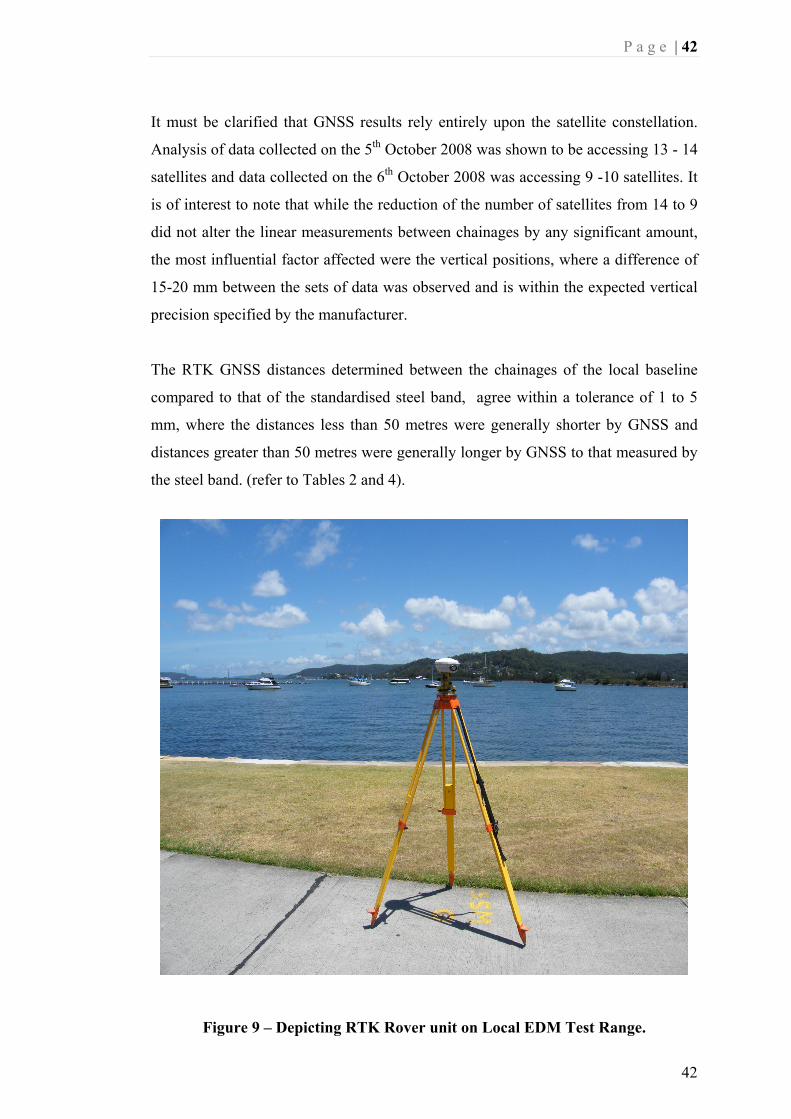
It must be clarified that GNSS results rely entirely upon the satellite constellation.
Analysis of data collected on the 5th October 2008 was shown to be accessing 13 - 14
satellites and data collected on the 6th October 2008 was accessing 9 -10 satellites. It
is of interest to note that while the reduction of the number of satellites from 14 to 9
did not alter the linear measurements between chainages by any significant amount,
the most influential factor affected were the vertical positions, where a difference of
15-20 mm between the sets of data was observed and is within the expected vertical
precision specified by the manufacturer.
The RTK GNSS distances determined between the chainages of the local baseline
compared to that of the standardised steel band, agree within a tolerance of 1 to 5
mm, where the distances less than 50 metres were generally shorter by GNSS and
distances greater than 50 metres were generally longer by GNSS to that measured by
the steel band. (refer to Tables 2 and 4).
Figure 9 – Depicting RTK Rover unit on Local EDM Test Range.

P a g e | 43
43
4.1.2 Analysis of Results The methods stated in Chapter three, are intended to provide the best possible
solution at the time of writing. The analysis of the data will assist in providing the
cross checking of results to confirm that in fact, the intended objectives and results
are being both met and achieved.
Given that this project will cover fairly new territory, it would appear difficult to
predict any firm outcome on the research topic. Preliminary investigation of data
analysis appears to highlight that the use of RTK GNSS derived measurements may
be able to calculate the additive constant of an EDM instrument, as the true distance
does not need to be defined nor proven to calculate this. The scale factor could be
determined as long as the use of a suitably known lineal length greater than 1000
metres is used (United States Department of Commerce 1994).
The EDM distances measured over the local test range agreed more closely to that of
the RTK GNSS derived distances, particularly over the longer distances. This
perhaps highlights the small additive errors associated with determining the lengths
and adding up those part lengths measured by the steel band. (refer Appendix B for
full results).
It was subsequently determined that the steel band measurements, particularly when
a length greater than 75 metres was needed, produced unreliable results. This may
be as a result of step chaining. The steel band measurements less than this distance
provided good agreement with those obtained by RTK GNSS. Noting this, a distance
of 75 metres would not provide enough redundant measurements to achieve the
purpose of this research and accordingly the steel band measurements will not be
used to determine the additive constant or scale factor of the EDM instruments, the
certified Newcastle EDM test line was used for that purpose.

P a g e | 44
44
Verification of measurement and the clarification of obtaining legal traceability for
GNSS measurements are dependent on the ensuing legislative requirements to be met
and subsequent verification of further testing and results which are likely to be
beyond the scope of this research project.
Figure 10 – Depicting RTK Base unit on Local EDM Test Range.

P a g e | 45
45
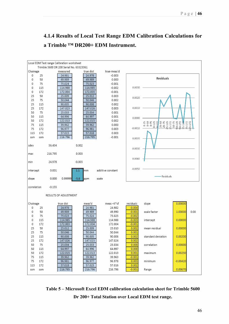
4.1.3 EDM Calibration Results
Using the mean of the two sets of RTK GNSS distances as being the ‘true distance’
for the local EDM test range, two different software methods were used to determine
the resulting additive constants and scale factors of a Trimble ™ 5600 DR200+ and
Topcon GPT6005 EDM instrument.
As the temperature and barometric pressure at the time of measurements resulted in
the parts per million (ppm) corrections being zero, no velocity or atmospheric
corrections were applied to the measured slope distances for the calibration
reductions.
The Microsoft ® Excel and ‘Calibrate’ EDM calibration calculation reduction sheets
and reports for the local EDM test range are shown in Appendices B and C.
Comparison of the local test range with the calibration results obtained over the
Newcastle EDM test line for the same EDM instruments highlight the significant
difference of the scale factor. This difference may be as a result of the different total
lengths of the local EDM test range and the certified Newcastle EDM test line.
Noting that, the certified EDM test line located at Wakefield, NSW has a total length
of 207 metres.
The residuals using Microsoft Excel for both EDM instruments calibrated over the
local EDM test range lie within the manufacturers stated accuracies for their
respective instruments. The only noticeable exception being from chainage 0 to 25
which was – 4 millimetres and thus is outside both of the instruments specifications.
P a g e | 46
46
4.1.4 Results of Local Test Range EDM Calibration Calculations for
a Trimble ™ DR200+ EDM Instrument.
Table 5 – Microsoft Excel EDM calibration calculation sheet for Trimble 5600
Dr 200+ Total Station over Local EDM test range.

P a g e | 47
47
For the Trimble ™ 5600 DR200+, the resulting additive constant calculated by
‘Calibrate’ software was determined to be +1.7mm.
Using the Microsoft ® Excel calculation spreadsheet, the additive constant was
determined to be +1.1 mm. Given that these were derived from two independent
sources and methods, the closeness of the two highlights the legitimacy of the results
(refer Appendix B).
The scale correction calculated by ‘Calibrate’ was determined to be -8.6 parts per
million (ppm). The calculated Microsoft ® Excel spreadsheet scale factor was
determined to be -5.6 (ppm). The two results contain a difference of 3 ppm.
For comparison purposes, the calibration results for this instrument, obtained over
the certified Newcastle EDM test line, determined an additive constant of +3.1 mm
and a scale factor of -1.5 (ppm).
Table 6 shows the results obtained for a Trimble ™ 5600 DR 200+ EDM instrument
over the certified Newcastle EDM test line. The additive constant and scale factor
errors have been determined, to enable the verification and certainty of measurement
in accordance with the Surveyor Generals Directions No. 5.
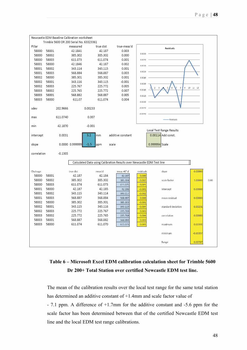
P a g e | 48
48
Table 6 – Microsoft Excel EDM calibration calculation sheet for Trimble 5600
Dr 200+ Total Station over certified Newcastle EDM test line.
The mean of the calibration results over the local test range for the same total station
has determined an additive constant of +1.4mm and scale factor value of
- 7.1 ppm. A difference of +1.7mm for the additive constant and -5.6 ppm for the
scale factor has been determined between that of the certified Newcastle EDM test
line and the local EDM test range calibrations.

P a g e | 49
49
4.1.5 Results of Local Test Range EDM calibration calculations for a
Topcon GPT6005 EDM Instrument.
Table 7 – Microsoft Excel EDM calibration calculation sheet for Topcon
GPT6005 Total Station over Local EDM test range.

P a g e | 50
50
For the Topcon GPT6005, the resulting additive constant calculated by ‘Calibrate’
software was determined to be -8.9 mm.
Using the Microsoft ® Excel calculation spreadsheet, the additive constant was
determined to be -8.7 mm respectively. Again the closeness of the two highlights the
legitimacy of the results given them being determined from two separate sources.
The scale correction calculated by ‘Calibrate’ was determined to be –10.5 parts per
million (ppm). The calculated Microsoft ® Excel spreadsheet scale was determined
to be -11.9 (ppm). The difference in the scale factor, in this instance for the two
results is 1.4 (ppm).
The calibration results obtained over the certified Newcastle EDM test line
determined an additive constant of -8.0 mm and a scale factor of +2.8 (ppm).
Table 8 shows the results obtained for a Topcon GPT6005 EDM instrument over
Newcastle EDM test line. The additive constant and scale factor errors have been
determined, to enable the verification and certainty of measurement in accordance
with the Surveyor Generals Directions No. 5.
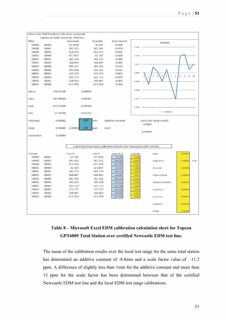
P a g e | 51
51
Table 8 – Microsoft Excel EDM calibration calculation sheet for Topcon
GPT6005 Total Station over certified Newcastle EDM test line.
The mean of the calibration results over the local test range for the same total station
has determined an additive constant of -8.8mm and a scale factor value of -11.2
ppm. A difference of slightly less than 1mm for the additive constant and more than
13 ppm for the scale factor has been determined between that of the certified
Newcastle EDM test line and the local EDM test range calibrations.

P a g e | 52
52
Chapter 5 Further Discussion 5.1 Discussion on EDM Calibration Results Currently, GNSS cannot be used to calibrate, verify or certify EDM devices. For this
to occur GNSS measurements essentially have to be identified as a value reference
standard and further, the accuracy and precision of GNSS derived measurements for
EDM calibration necessitates the need for millimetre accuracy up to the range
whereby EDM is required to be used for survey related tasks.
Beyond the extent of which an EDM device is calibrated, GNSS is highly likely to be
able to provide a linear distance within the scope of an EDM manufacturers stated
tolerance. In other words, there would be a convergence whereby the two devices,
being GNSS and EDM meet in terms of their respective stated accuracies. Beyond
that, there is a valid argument whereby GNSS would likely provide better accuracy
and precision over longer linear distances to that of an EDM instrument due to
EDM’s manufacturing limitations and accuracies.
While some evidence exists that GNSS is able to perform well within the scope of
the manufacturers stated accuracy, it still falls well short of that required to ascertain
the EDM calibration errors required for its verification as highlighted by the
variations of the RTK GNSS measurements observed over the local test range. It has
been previously determined that the absolute or known distances are not required to
enable the calculation of an EDM instruments additive constant. However the scale
factor component relies heavily on true distances and atmospheric conditions being
accurately determined as well as a linear length of 1000 metres or more.

P a g e | 53
53
At the time of writing, the results obtained from RTK observations on a certified
EDM calibration baseline, provided sufficient insight and evidence insofar as the
continuing and ongoing improvement of GNSS equipment and the linear distances
derived from it.
Table 9 provides a comparison of results between the linear distances published for
inter-pillar distances over the Newcastle EDM baseline by the NSW Department of
Lands, with that derived from three minute control point RTK GNSS observations.
Table 9 - Comparison of Trimble ™ R8 RTK GNSS observations over
Newcastle EDM test line for verification of equipment.
RTK GNSS Mga coords by RTK GNSS
RTK Distances measured against true published distances
EAST NORTH MARK
RTK GNSS ground distances
Published True DISTANCE
True –meas’d
Pm 58000 (p1) 379022.3670 6360098.5600 p1 - p2 42.187 42.187 0.000 pm 58001 (p2) 379055.5200 6360072.4880 pm 58002 (p3) 379325.2000 6359860.4540 p1 – p4 611.070 611.074 -0.004 pm 58003 (p4) 379502.6220 6359720.9480
CHK 58000 379022.3700 6360095.5640 p2 - p4 568.883 568.887 -0.004 CHK 58002 379325.1990 6359860.4400 CHK 58003 379502.6230 6359720.9520
p1chk - p2 42.187 42.187 0.000
p1chk - p4 611.070 611.074 -0.004
comments p1chk - p4 chk 611.068 611.074 -0.006
pm58002 badly covered by trees. p1 - p4chk 611.067 611.074 -0.007
p2 - p1chk 42.187 42.187 0.000
p2 -p4chk 568.880 568.887 -0.007

P a g e | 54
54
It must be reiterated that Pillar 3 (PM 58002) on the Newcastle EDM baseline is
highly unsuitable for GNSS derived measurements due to site constraints, and
accordingly would not fall into the category of best practice as defined in the SP1
manual as published by ICSM for observations and recommended procedures.
It was made evident in my personal communications in August 2008 with Mr Robert
Lock, chief legal metrologist of the Department of Lands NSW, that this particular
monument (PM 58002) has been determined to be situated over a large water main
pipe and that he has noticed that the pillar is actually moving overtime. A recent
study has been undertaken by Sam Nicoll, a student at the University of Newcastle
on the movements of the Newcastle EDM baseline.
What the use of this certified baseline does highlight, is that the RTK GNSS
comparisons observed between the baseline pillars, in this instance, add further
weight to the hardware and software updates continually being implemented and put
in place by equipment manufacturers to make GNSS much more ideal in its uses
beyond its currently viewed capacity. Naturally, further and much more extensive
research would be required to be able to substantiate this claim and provide proof of
the same.
The purpose of the exercise of measuring and verifying the GNSS equipment over
the Newcastle EDM test line was purely fundamental in enabling a direct comparison
of the results being able to be shown to that of a verified and certified legally
traceable source of measurement. The Newcastle EDM test line alone could not be
relied upon to support the viability of this project.
P a g e | 55
55
Chapter 6 Consequential Effects and Ethical Responsibility 6.1 Implications The issue with resolving the additive constant and scale factor errors of an EDM
instrument is that millimetre accuracy is essential and is required to determine this.
In lieu of that, it is commonly known that the general specifications for RTK
measurements with GNSS equipment is +/- 10mm + 1 part per million (ppm). Given
this, the specifications endorsed by the manufacturer are based on the operating
range of the equipment which is -20 deg centigrade up to +50 deg centigrade.
Put simply, while an additive constant and scale factor of two different EDM
instruments was able to be calculated from the GNSS derived local EDM test range,
GNSS cannot be used to provide calibration of EDM with legal traceability.
In my research for this project and practical surveying experience, I have concluded
that measurements derived from RTK GNSS positions, will generally be of much
better accuracy than those implied by the manufacturer’s specifications. An example
of this, shown in Table 9, shows that at the certified Newcastle EDM calibration
baseline data from a Trimble ™ R8 GNSS RTK system was recorded by inter-pillar
measurements in the same method as an EDM instrument would be used for
calibration purposes. This baseline may not continue to be a reference source for
obtaining measurements by GNSS due to increasing vegetation that may restrict
satellite visibility. However, the current results obtained do highlight the
improvement in software enhancements which are able to take into account factors
such as multipath and ambiguities from short observation times, particularly with
regard to RTK GNSS observations.
P a g e | 56
56
This project aimed to investigate and cover all possible alternatives to derive a
deemed correct result and/or recommendation. It cannot be emphasised more
strongly, that an element of doubt may be present in achieving either the same or a
similar result with equipment from a different manufacturer than the ones used in this
project or under different conditions to that undertaken at the time. Further scrutiny
of results and methods and future changes in technological advances, may logically
provide an alternative solution to that which this project concludes.
This project intended to achieve an outcome as stated in the ‘Project Aim’ which was
to use RTK GNSS to calibrate an EDM instrument to determine its errors and
provide legal traceability of its measurement.
The value of this project is to assist the Surveying industry in providing a solution to
EDM calibration and verification without utilising the current requirement of
measuring their equipment over a currently certified EDM baseline.
It is suggested that with the GNSS system and the associated technology being
constantly upgraded and improved, better accuracy may well be achieved in the
positions obtained and the resultant measurements determined with millimetre
accuracy.
Other documentation has shown that GNSS over large distances achieves much
better results than that obtained from the previous trilateration and triangulation
methods of coordinating the state network used in the late 19th Century.
It is of interest that although GNSS technology continues to improve, the
methodologies and the ideologies of techniques other than that currently being used
are often challenged and subject to scepticism. This will continue until there is an
acceptance of GNSS as a ‘best practice’ method of measurement.

P a g e | 57
57
As to what timeframe one places on GNSS becoming a suitable and reliable value
reference standard, able to be easily replicated anywhere on the earth or in space at
any time on any day is unknown. However, as technology advances, the future of
using GNSS with complete confidence and reliability may be closer than anticipated.
The issue and ongoing requirements of EDM verification and calibration will not
change, but with GNSS equipment becoming more common in the standard survey
practice, it would be appropriate to determine suitable methods and provide a
solution whereby GNSS can be utilised to undertake such continuing requirements.
The additive constant and the scale factor errors in EDM instruments are usually
resolved over a certified EDM baseline. The cyclic error can be determined by
measurements by EDM of 1 metre intervals using a standardised tape to set the
graduations that will be compared to. Accordingly, GNSS would not be required to
determine this error. Only the additive constant and scale factor would be required to
be determined by GNSS, and only when all three errors have been solved will legal
traceability of the EDM device be achieved.

P a g e | 58
58
6.2 Risk Assessment The majority of testing for this project involves field surveying, both within private
property and public roads/reserves. With regard to Occupational Health and Safety,
there is an inherent risk factor associated with carrying out the usual survey tasks and
procedures. Specific risk assessment for the tasks involved in this project have been
identified and documented hereon:
Safe Work Method Statement
Risk Assessment
Risk Break the job down
into steps
Potential Hazard And Severity.
What can harm you?
Controls What you are going to do to make the job as safe as possible
1 Lifting theodolite & gear from vehicle
Lifting - back strain
(Low)
* Use correct lifting procedures.
2 Setting up instrument / tripod on footpath and/or accessways.
* Collisions with pedestrians
* Trip/fall injury
(Moderate)
* Use witches hats to provide protective
barrier around work station
* Wear reflective jackets
3 Walking between stations / tripods/
work area.
* Sun Exposure
* Trip/fall injury
(Low)
* Wear protective footwear, reflective jackets, headwear, eyewear and sun
lotion 4 Working in vicinity of
vehicles. Serious injury/ Death
(High)
* Wear reflective jackets, place
witches hats around equipment
* Park vehicle next to kerb as barrier
* Use warning signs
& traffic control to AS 1742.3

P a g e | 59
59
5 Working with Laser Equipment - Class 2
and above.
Serious Eye Damage
(Moderate)
* avoid looking directly at beam.
6 Working with controllers/computers
in field
Eye strain/ fatigue
(Low)
* ensure adequate protection from
sunlight. * Take regular breaks.
7 Working with computers in Office
Eye strain/ fatigue Muscle strain
(Low)
* Take regular breaks. * Ensure good posture.
8 Using levelling staff. Electrical shock – level staff hits
overhead power lines.
(High)
* Look up. Adopt route for levelling away from power lines. Keep staff at least 8
metres clear of all overhead lines.
9 Working alone on site. Dehydration, loss of contact with office
and missing.
(Moderate)
* Carry bottled water (2 litres).
* Carry mobile phone. * Report back to office at
regular intervals. 10 Using spray paint. Paint in eyes or hands.
(Low)
Wear P.P.E – goggles on eyes, disposable gloves on hands.

P a g e | 60
60
Chapter 7 Summary and Conclusion 7.1 Summary
The preceding chapters have identified and highlighted the problems at hand and the
constraints to be addressed with regard to the validity of this project.
Notwithstanding, some of these issues are required to be addressed and amended.
A Trimble 5600 DR200+ EDM instrument that was calibrated over the certified
Newcastle EDM test line has been determined to have an additive constant of +3.1
mm and scale factor of -1.5 ppm.
The results for this same EDM instrument over the local test range using Microsoft
Excel have determined an additive constant of +1.1 mm and scale factor of -5.6 ppm.
‘Calibrate’ software determined an additive constant of +1.7 mm and scale factor of -
8.6 ppm. The manufacturer’s specification for this particular EDM instrument that
was used in the calibrations is +/- 3 mm + 3 ppm (Trimble).
A Topcon GPT6005 EDM instrument calibrated over the certified Newcastle test line
has been determined to have an additive constant of -8.0 mm and scale factor of +2.8
ppm.
The results over the local test range for this instrument using Microsoft Excel has
calculated an additive constant of – 8.7 mm and scale factor of – 11.9 ppm.
‘Calibrate’ software calculated an additive constant of -8.9 mm and -10.5 ppm. The
manufacturer’s specification for this instrument is +/- 3 mm + 2 ppm (Topcon).

P a g e | 61
61
7.2 Recommendations
The use of GNSS is likely to become a viable proposition for undertaking the
calibration of EDM devices. At this stage, GNSS does not provide legal traceability
for the verification of an EDM device. When GNSS may actually be able to achieve
this is possibly being fast tracked into fruition by many of the recognised leading
authorities around the world.
RTK GNSS is deemed to be less accurate than the use of the fast-static method of
data collection. For the purpose of this research, the recommendations for the use of
GNSS to determine linear distances are as follows:
• The GNSS equipment should be of geodetic quality and verified against
either the State Control Network with published three dimensional values or
over an existing certified EDM test line suitable for GNSS observations.
• At least two different independent sets of observations should be recorded to
confirm consistency of results for the establishment of any distance.
• Seven or more satellites will enable better precision and accuracy as long as
the geometry of the satellite constellation and the precision of the data are
investigated with the proper planning methods undertaken to achieve this.
• An EDM instrument calibrated over any GNSS derived baseline should still
be undertaken in accordance with the current methods used, including the
recording of temperature, barometric pressure and repetitive individual
measurements.
• Any GNSS derived EDM calibration baseline should be directly tied to the
State Survey Control Network to add further weight to the validity of the
GNSS derived measurements.

P a g e | 62
62
As highlighted in this research, the scale factor component of the EDM calibration
was the most difficult to determine. Where GNSS is likely to be of most use in
determining this would be in rural surveys where a GNSS baseline of 1000 metres or
more could be created and an EDM instrument measure over this baseline for
comparison. Once a scale is determined based on the GNSS distance divided by the
EDM measured, comparison could be made as to whether the EDM device is
measuring within its manufacturer stated accuracies. i.e. +/- 3mm + 5ppm.
For an Urban environment, connection of an EDM device to the State Survey
Control Network is likely to provide a comparison of measurement to the published
values for the determining of the EDM instrument measuring within the instruments
specifications.
Noting the above, any EDM instrument should be verified over a calibrated EDM
baseline at least once to enable a record of legally traceable measurements to be
created. Once the additive constant and scale factor errors of an instrument are
known, GNSS may provide a useful tool for monitoring an EDM’s calibration by a
user setting up their own EDM test range using GNSS similar to that undertaken in
this project and regularly measuring their EDM over this. This monitoring method
would provide a much more convenient method of EDM verification to that currently
required.

P a g e | 63
63
7.3 Conclusion
When the use of EDM equipment became accepted within the surveying profession,
legal traceability was implemented. The same idealistic approach needs to be
replicated with GNSS to enable measurements to be legally traceable.
The fundamental purpose of using GNSS to create a local test range is to enable the
traceability of an EDM instrument back to a primary standard. This research has
shown that RTK GNSS can provide measurements better than the manufacturers
stated accuracies, and, furthermore can provide some element of its measurements
being legally traceable by proving a fairly consistent comparison of length to that of
the State Survey Control Network published values.
This project was able to calibrate two different EDM instruments over a local test
range derived from RTK GNSS and an existing certified EDM baseline to determine
the additive constant and scale errors and determine the validity of the RTK GNSS
method used in this research.
Legislative changes are required and the adoption of GNSS being recognised as a
legally traceable method of measurement in the same way that EDM had become
needs to occur. This research highlights that GNSS is a valuable survey tool for
measurement and priority should be given to GNSS having legal traceability.
Finally, this project was not able to provide legal traceability of the measurements
and verification of the local GNSS derived EDM test range. Other than having a
comparison with the State Survey Control Network and the known errors of the
EDM instruments determined over the certified Newcastle EDM test line, it is
unclear what other requirements are to be undertaken to ‘legally trace’ the GNSS
linear measurements for this local EDM test range.

P a g e | 64
64
7.4 Further Work
For New South Wales, GNSS measurements are not legally traceable to a reference
value standard unless those measurements are directly tied to the AFN or ARGN.
With the continual improvement and technological advances in both hardware and
software of GNSS systems, there would exist a strong argument that GNSS
equipment, once verified and validated, could be used to undertake surveys and
further too, enable the provision of legally traceable measurements similar to that
achieved by the using of conventional measurement devices.
The current legislation for GNSS traceability lies in the hands of the New South
Wales Surveyor General and the ICSM. As both are currently approved as legal
verifying authorities under the provisions of Regulation 73 of the National
Measurement Act 1960, the onus and responsibility of validating GNSS with legal
traceability lies within their realm.
The issue of legal traceability of GNSS derived measurements has been well
documented by this and other previous research.
The use of the RTK method of obtaining GNSS measurements is recognised not to
be the most reliable nor accurate method of obtaining data. Fast Static (post
processed) observations are likely to yield better results and may provide further
insight as to the validity of this method of providing EDM calibration and
verification.
Once the advancements and innovations associated with GNSS technology are able
to provide greater accuracy than that currently available and actually become legally
traceable, more research into the viability of using GNSS will be further warranted
and justifiably needed.

P a g e | 65
65
While an additive constant and scale factor for an EDM device was able to be
determined over the local EDM test range, this research has highlighted that the scale
factor component of an EDM instrument is the most difficult to determine and a
recommendation for further research to investigate determining the scale factor by
GNSS measurements be undertaken over much longer linear lengths than that used in
this project.
The relevance of this research being further pursued is of great benefit to the
surveying industry as a means of providing an alternative method for a solution to
EDM calibration and traceability of measurement in accordance with the National
Measure Act 1960 and the relevant International Standards.
P a g e | 66
66
References
Bannister. A., Raymond. S. and Baker. R. 1998. “Surveying”, 7th Edition, Pearson
education Ltd, England, 1998.
BIPM -“The BIPM and the evolution of the definition of the metre”, Bureau
International des Poids et Mesures - BIPM website, accessed on 12th May 2008.
http://www.bipm.org/en/si/history-si/evolution_metre.html
Brunner, F. K. and Rüeger, J. M. 1992. "Theory of the Local Scale Parameter
Method for EDM". Bulletin Géodésique, 66 (1992): 355-364.
Ciddor, P.E. 1999. “GPS Surveying: A Traceability Chain with a missing link”.
CSIRO National Measurement Laboratory, Lindfield, Australia.
Commonwealth of Australia (1960) “National Measurement Act 1960”, Australian
Government Publishing Service, Canberra, Australia.
Commonwealth of Australia 2008, “Australian Fiducial Network”, Geoscience
Australia website accessed on 24 May 2008.
http://www.ga.gov.au/geodesy/argn/afngiff.jsp
Department of Sustainability and the Environment, Victoria. “EDM Calibration
Handbook – V9, 2007”. Lands, Victoria website accessed 12 October 2008.
http://www.land.vic.gov.au/CA256F310024B628/0/2AC14DC8753E005DCA25733
9000516E3/$File/EDM+Handbook+V9.0.pdf
.
Featherstone, W.E., Forward. T.A., Penna. N., Stewart. M.P., Tsakiri. M., McCarthy.
R.., Houghton. H. and Xanthis. G. (2001) “Establishment of GNSS testing and
validation facilities in Perth, Western Australia”, in: Kubik, K., C. Rizos and W.E.
Featherstone (eds) Proceedings of SatNav 2001, 5th International Symposium on
Satellite Navigation Technology and Applications, Canberra, Australia, July.

P a g e | 67
67
Gibbings. P., 2002. “The Design of Interactive Web-based GPS training”, University
of Southern Queensland, Toowoomba
Hale. M., Ramm. P., and Wallace. J. 2007. “Legal Positions and Victoria’s
GPsNet”, Spatial Science Conference (SSC2007), Hobart, Tasmania, Australia.
Higgins. M. B. 2001. “Guidelines for GPS Surveying in Australia” FIG Working
Week 2001, Seoul, Korea May 2001. http://geodesia.ufsc.br/Geodesia-
online/arquivo/FIG/2001%20Seul/ws_com5_1/higgins.htm
Intergovernmental Committee on Surveying and Mapping, (ICSM) website.
“Active GPS and Survey Marks” paper prepared by ICSM Geodesy Group 2008.
Accessed on 12 September 2008.
http://www.icsm.gov.au/icsm/publications/gtsc/ActiveGPSAndSurveyMarks.pdf
Intergovernmental Committee on Surveying and Mapping, (ICSM) website.
“Standards and Practices for Control Surveys (SP1) Version 1.7”, accessed on 22
May 2008. http://www.icsm.gov.au/icsm/publications/sp1/sp1v1-6.pdf
ISO (International Organisation for Standardization) First Edition 2002-03-15.
“Optics and optical instruments – Field procedures for testing geodetic and
surveying instruments – Part 4: Theory. ISO 17123-1:2002(E)”. viewed 22 May
2008.
ISO (International Organisation for Standardization) First Edition 2001-12-01.
“Optics and optical instruments – Field procedures for testing geodetic and
surveying instruments – Part 4: Electro-optical distance meters (EDM
instruments)”. ISO 17123-4:2001(E). viewed 23 May 2008.
ISO (International Organisation for Standardization) First Edition 2007-09-15.
“Optics and optical instruments – Field procedures for testing geodetic and
surveying instruments – Part 8: GNSS field measurement systems in real-time
kinematic (RTK)’. ISO 17123-8:2007(E). viewed 23 May 2008.

P a g e | 68
68
Khalil, Dr. Ragar. 2005. “New Compact Method for Laboratory Testing EDM
Instruments”. Fig Working Week 2005 and GSDI-8, Cairo, Egypt. April, 2005.
New South Wales Government, Department of Lands NSW website. Last accessed
on the 20th October 2008. http://www.lands.nsw.gov.au/
New South Wales Government, Surveyors Generals Directions No. 5 – “Verification
of Distance Measuring Equipment”, December 2004.
New South Wales Government, Surveyors Generals Directions No. 9 –
“GPS Surveys”, December 2004.
Ollis, J. 2007. “A Reflective Look at the Calibration of EDM Instruments”. Institute
of Surveyors NSW, Azimuth No. 45, Issue 2, (p 27, 30 – 31).
Parker, R, Ramm, P and Fennel, A. 1998. “Cadastral Reform in Victoria, Australia”.
Accessed on 25 May 2008.
http://www.sli.unimelb.edu.au/fig7/Brighton98/Comm7Papers/TS34-
Parker/PAPER.html
Rüeger, J.M., 1980. “Legal Requirements for the Calibration of EDM-Instruments”.
Proc., 22nd Australian Survey Congress, Hobart, 1980, 10-1-10-10.
Rüeger, J.M., 1977. “Design and Use of Baselines for the Calibration of EDM-
Instruments”. Proc., 20th Australian Survey Congress, Darwin, 175-189.
Rüeger, J. M., 1984. “Instructions on the Measurement of Subsidiary Standards of
Length in the form of EDM Calibration Baselines using Distance Meters as
Prescribed by the National Standards Commission”. August 1984, 21 pages.
Rüeger, J. M., 1991. “Legal Calibration of Electronic Distance Meters in Australia”.
The Australian Surveyor, 36(3): 195-212.
Rüeger, J. M., 1996. “Electronic Distance Measurement - An Introduction. Fourth
corrected edition”. Springer-Verlag, Berlin-Heidelberg-New York, 276 pages.

P a g e | 69
69
Rüeger, J. M. 2003. “Electronic Surveying Instruments - A Review of Principles,
Problems and Procedures”, 1st ed. School of Surveying and Spatial Information
Systems, University of New South Wales, Sydney, Australia, 156 pages.
SAI GLOBAL – “Standards Australia Website”. Accessed via the University of
Southern Queensland, last accessed on 22 May 2008.
http://www.saiglobal.com.ezproxy.usq.edu.au/online/autologin.asp
The International Laboratory accreditation cooperation (ILAC). “ILAC Policy No.10
on Traceability of Measurement Results”, viewed 22 July 2008.
http://www.ilac.org/documents/ILAC_P10_2002_ILAC_Policy_on_Traceability_of_
Measurement_Result.pdf
Trimble Survey and Research White Papers – “Defining the future of satellite
surveying with Trimble R-Track technology, 2006”, Trimble website accessed on 22
May 2008.http://trl.trimble.com/docushare/dsweb/Get/Document-287233/022543-
214_GNSS_WP_0206_Survey.pdf
Unites States of America, Dept of Commerce NOAA Technical Memorandum NOS
NGS 8 - “Establishment of Calibration Base Lines, 1994”, National Geodetic
Survey Website accessed on 28 September 2008.
http://www.ngs.noaa.gov/PUBS_LIB/TMNOSNGS8.pdf
Wells, D.E., N. Beck, D. Delikaraoglou, A. Kleusberg, E. J. Krakiwsky, G.
Lachapelle, R. B. Langley, M. Nakiboglu, K. P. Schwarz, J. M. Tranquilla, and P.
Vanĩcek (1986). “Guide to GPS Positioning”. Department of Geodesy and
Geomatics Engineering Lecture Note No. 58, University of New Brunswick,
Fredericton, New Brunswick, Canada, 291 pp. accessed on 22 May 2008.
http://gauss.gge.unb.ca/Guide_to_GPS_Positioning.html
P a g e | 70
70
Appendix A – Project Specification……………….……………………71
Appendix B –Calculation sheets and report - Trimble EDM……72
Appendix C – Calculation sheets and report – Topcon EDM….74
Appendix D – Scale factor calculation sheet for Local Test
Range…………………………………………………………………………...76
Appendix E – Trimble Raw Data File 05/10/2008…………………77
Appendix F – Trimble Planning Software DOP Values….………84
Appendix G – Trimble Raw Data File 06/10/2008….….….……....86
Appendix H – Trimble Planning Software DOP Values………...93
Appendix I – Trimble 5600 Data Sheet………………….…………....95
Appendix J – Trimble R8 GNSS Data Sheet………………………..98
Appendix K – Topcon GPT6005 Data Sheet……………….……....100
Appendix L – SCIMS Survey Mark Data…………………………...101

P a g e | 71
71

P a g e | 72
72
Appendix B

P a g e | 73
73

P a g e | 74
74
Appendix C
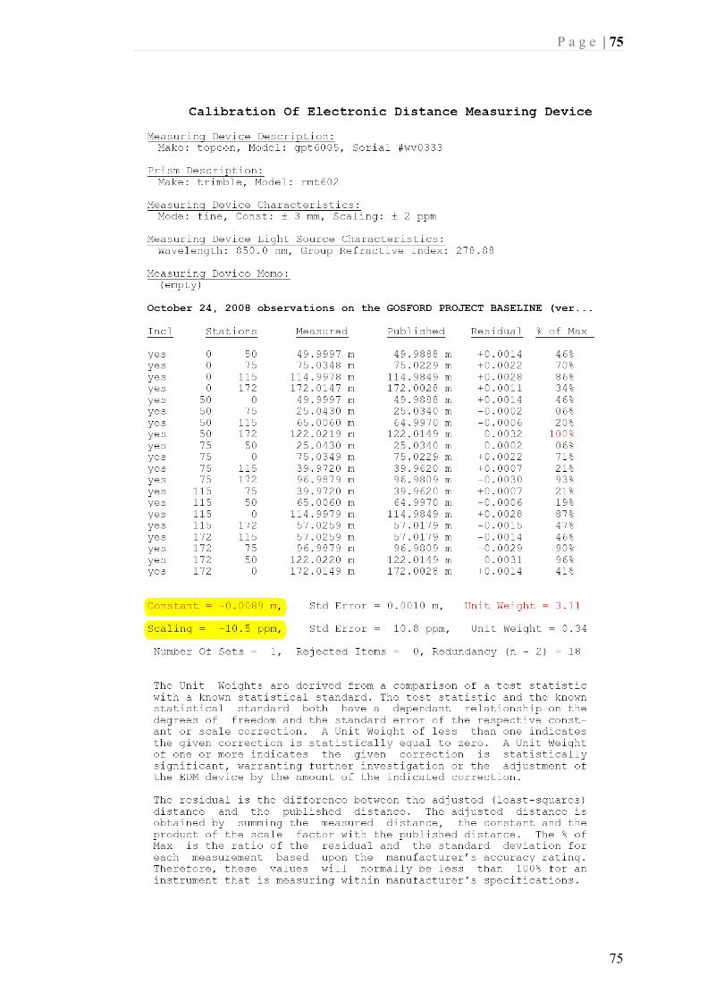
P a g e | 75
75

P a g e | 76
76
Appendix D
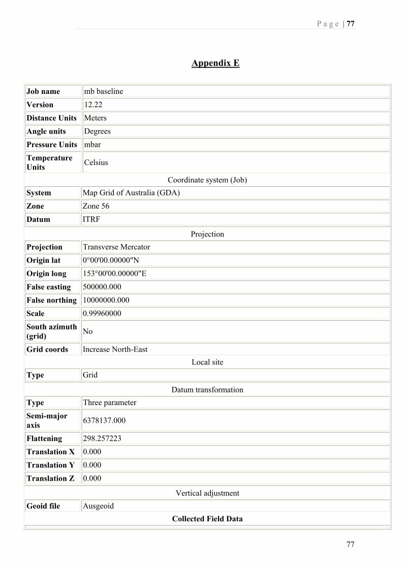
P a g e | 77
77
Appendix E
Job name mb baseline
Version 12.22
Distance Units Meters
Angle units Degrees
Pressure Units mbar
Temperature Units Celsius
Coordinate system (Job) System Map Grid of Australia (GDA)
Zone Zone 56
Datum ITRF
Projection Projection Transverse Mercator
Origin lat 0°00'00.00000"N
Origin long 153°00'00.00000"E
False easting 500000.000
False northing 10000000.000
Scale 0.99960000
South azimuth (grid) No
Grid coords Increase North-East Local site
Type Grid
Datum transformation Type Three parameter
Semi-major axis 6378137.000
Flattening 298.257223
Translation X 0.000
Translation Y 0.000
Translation Z 0.000
Vertical adjustment Geoid file Ausgeoid
Collected Field Data
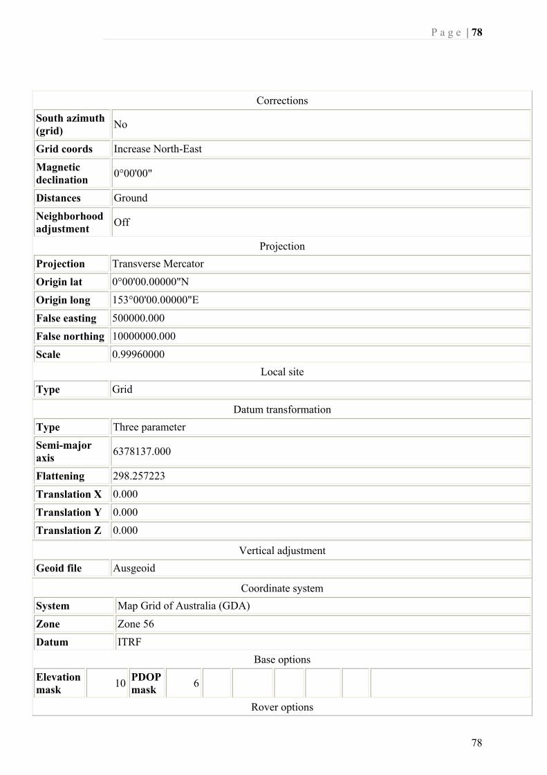
P a g e | 78
78
Corrections
South azimuth (grid) No
Grid coords Increase North-East
Magnetic declination 0°00'00"
Distances Ground
Neighborhood adjustment Off
Projection Projection Transverse Mercator
Origin lat 0°00'00.00000"N
Origin long 153°00'00.00000"E
False easting 500000.000
False northing 10000000.000
Scale 0.99960000 Local site
Type Grid
Datum transformation Type Three parameter
Semi-major axis 6378137.000
Flattening 298.257223
Translation X 0.000
Translation Y 0.000
Translation Z 0.000
Vertical adjustment Geoid file Ausgeoid
Coordinate system System Map Grid of Australia (GDA)
Zone Zone 56
Datum ITRF Base options
Elevation mask 10 PDOP
mask 6 Rover options

P a g e | 79
79
Elevation mask 10 PDOP
mask 6 Survey event
Survey event Base started Initialization event: Gained
GPS week 1500 Seconds 8221 Initialization
type
On the fly
Surveytype
Real-time
Initialization count 1
GPS receiver Receiver type R8-2
Serial number 4803143857
Firmware version 3.62
Antenna type R8 Model 2/SPS88x Internal
Measurement method Center of bumper
Tape adjustment 0.000
Horizontal offset 0.091
Vertical offset 0.010
Point 2 ∆X -5.784 ∆Y 15.047 ∆Z 19.080 Code ch25
Antenna height 1.700 Type Uncorrected Hz Prec 0.002 Vt
Prec 0.003
QC 1 Satellites 12 PDOP 0.6 HDOP 0.4 VDOP 0.5
RMS 10.035 Positions used 187
Std. Dev (H)
? Std. Dev (V)
?
QC 2 Satellites 13 VCV xx (m²) 0.000008
VCV xy (m²)
-0.000002
VCV xz (m²)
0.000001
Error scale (m) 0.010
VCV yy (m²)
0.000003 VCV yz (m²)
-0.000001
VCV zz (m²)
0.000003
Point 3 ∆X -11.741 ∆Y 30.171 ∆Z 38.087 Code ch50
Antenna height 1.700 Type Uncorrected Hz Prec 0.003 Vt
Prec 0.003 QC 1 Satellites 13 PDOP 0.7 HDOP 0.5 VDOP 0.5
RMS 15.849 Positions used 183 Std.
Dev ? Std. Dev ?

P a g e | 80
80
(H) (V)
QC 2 Satellites 13 VCV xx (m²) 0.000010
VCV xy (m²)
-0.000003
VCV xz (m²)
0.000001
Error scale (m) 0.010
VCV yy (m²)
0.000003 VCV yz (m²)
-0.000002
VCV zz (m²)
0.000004
Point 4 ∆X -17.786 ∆Y 45.365 ∆Z 57.044 Code ch75
Antenna height 1.735 Type Uncorrected Hz Prec 0.003 Vt
Prec 0.003
QC 1 Satellites 13 PDOP 0.7 HDOP 0.5 VDOP 0.5
RMS 9.506 Positions used 185
Std. Dev (H)
? Std. Dev (V)
?
QC 2 Satellites 13 VCV xx (m²) 0.000011
VCV xy (m²)
-0.000003
VCV xz (m²)
0.000001
Error scale (m) 0.010
VCV yy (m²)
0.000003 VCV yz (m²)
-0.000002
VCV zz (m²)
0.000004
Point 5 ∆X -27.316 ∆Y 69.555 ∆Z 87.389 Code ch115
Antenna height 1.712 Type Uncorrected Hz Prec 0.003 Vt
Prec 0.004 QC 1 Satellites 12 PDOP 0.8 HDOP 0.5 VDOP 0.6
RMS 14.786 Positions used 184
Std. Dev (H)
? Std. Dev (V)
?
QC 2 Satellites 13 VCV xx (m²) 0.000013
VCV xy (m²)
-0.000005
VCV xz (m²)
0.000001
Error scale (m) 0.010
VCV yy (m²)
0.000004 VCV yz (m²)
-0.000001
VCV zz (m²)
0.000003

P a g e | 81
81
Initialization event: High RMS
GPS week 1500 Seconds 9412 Initialization
type
On the fly
Survey type
Real-time
Initialization count 1
Initialization event: Good RMS
GPS week 1500 Seconds 9413 Initialization
type
On the fly
Survey type
Real-time
Initialization count 1
Point 6 ∆X -40.898 ∆Y 104.065 ∆Z 130.704 Code ch172
Antenna height 1.712 Type Uncorrected Hz Prec 0.002 Vt
Prec 0.004
QC 1 Satellites 14 PDOP 0.8 HDOP 0.4 VDOP 0.6
RMS 13.429 Positions used 182
Std. Dev (H)
? Std. Dev (V)
?
QC 2 Satellites 14 VCV xx (m²) 0.000010 VCV
xy (m²)-
0.000005
VCV xz (m²)
0.000002
Error scale (m) 0.010
VCV yy (m²) 0.000005
VCV yz (m²)
-0.000002
VCV zz (m²)
0.000003
Point 7 ∆X -48.008 ∆Y 135.142 ∆Z 162.580 Code SSM 100553
Antenna height 1.718 Type Uncorrected Hz Prec 0.002 Vt
Prec 0.004
QC 1 Satellites 14 PDOP 0.8 HDOP 0.4 VDOP 0.7
RMS 18.555 Positions used 195
Std. Dev (H)
? Std. Dev (V)
?
QC 2 Satellites 14 VCV xx (m²) 0.000009
VCV xy (m²)
-0.000006
VCV xz (m²)
0.000002
Error scale (m) 0.010
VCV yy (m²)
0.000006 VCV yz (m²)
-0.000002
VCV zz (m²)
0.000003

P a g e | 82
82
Survey event Survey event End survey
Rover options Elevation mask 10 PDOP
mask 6 Base options
Elevation mask 10 PDOP
mask 6 Base options
Elevation mask 10 PDOP
mask 6 Survey event
Survey event Base started GPS receiver
Receiver type R8-2
Serial number 4814150045
Firmware version 3.62
Antenna type R8 Model 2/SPS88x Internal
Measurement method Center of bumper
Tape adjustment 0.000
Horizontal offset 0.091
Vertical offset 0.010 Post processing file
File name 91922790.t01 Started
GPS week 1500 Seconds 10836
Survey event Survey event End survey
Projection Projection Transverse Mercator
Origin lat 0°00'00.00000"N
Origin long 153°00'00.00000"E
False easting 500000.000
False northing 10000000.000

P a g e | 83
83
Scale 0.99960000 Local site
Type Grid
Coordinate system System Map Grid of Australia (GDA)
Zone Zone 56
Datum ITRF Survey Controller Reduced Points
Point 1 East 345651.038 North 6299638.427 Elevation 6.748 Code SSM 100552
Point 2 East 345640.248 North 6299660.950 Elevation 6.667 Code ch25
Point 3 East 345629.474 North 6299683.517 Elevation 6.609 Code ch50
Point 4 East 345618.680 North 6299706.103 Elevation 6.638 Code ch75
Point 5 East 345601.449 North 6299742.152 Elevation 6.604 Code ch115
Point 6 East 345576.859 North 6299793.593 Elevation 6.498 Code ch172
Point 7 East 345552.395 North 6299831.454 Elevation 6.576 Code SSM 100553

P a g e | 84
84
Appendix F
Planning: List of DOP values
www.trimble.com Planning / Copyright (C) 2001 - 2008 by Trimble Navigation Limited.Station name Default
Latitude 33° 25'
Longitude 151° 20'
Height 2 [m]
Time span 5/10/2008/9:00:00 AM - 6/10/2008/9:00:00 PM
Time zone AUS Eastern Standard Time (DST)
Offset UTC +11.0 [h]
Elevation cut off 10°
Obstruction Editor 0%
GPS Satellites 2 3 4 6 7 8 9 10 11 12 13 14 15 16 17 18 19 20 21 22 23 24 25 26 27 28 29 30 31 32
Glonass Satellites 4 6 7 9 10 11 13 14 15 17 19 20 23 24
Galileo Satellites - none -
Compass Satellites - none -
Time GDOP TDOP PDOP HDOP VDOP GPS GLN GAL COM Total09:00 2.03 1.39 1.48 0.80 1.24 10 3 0 0 13 09:30 2.91 2.02 2.10 0.96 1.87 8 3 0 0 11 10:00 2.29 1.53 1.70 0.81 1.50 9 3 0 0 12 10:30 1.82 1.15 1.41 0.74 1.20 10 3 0 0 13 11:00 1.74 1.06 1.38 0.77 1.15 11 3 0 0 14 11:30 1.97 1.20 1.56 0.94 1.24 9 4 0 0 13 12:00 2.92 1.93 2.18 1.04 1.92 8 3 0 0 11 12:30 2.93 1.90 2.22 0.91 2.03 8 4 0 0 12 13:00 2.29 1.43 1.79 0.80 1.60 8 5 0 0 13 13:30 1.61 0.93 1.32 0.61 1.17 10 6 0 0 16 14:00 1.69 0.96 1.39 0.63 1.24 9 6 0 0 15 14:30 3.43 2.12 2.69 0.99 2.50 6 5 0 0 11 15:00 2.43 1.50 1.91 0.91 1.69 7 4 0 0 11 15:30 1.93 1.18 1.53 1.01 1.14 8 3 0 0 11 16:00 2.47 1.78 1.71 0.93 1.44 9 1 0 0 10 16:30 2.66 1.66 2.08 1.02 1.82 7 2 0 0 9 17:00 2.34 1.49 1.80 0.94 1.53 8 2 0 0 10 17:30 2.11 1.35 1.62 0.95 1.31 8 2 0 0 10 18:00 2.09 1.41 1.54 0.98 1.19 9 2 0 0 11 18:30 2.55 1.76 1.84 1.05 1.52 9 3 0 0 12 19:00 2.22 1.39 1.73 0.89 1.49 10 3 0 0 13 19:30 2.14 1.29 1.71 0.86 1.48 11 4 0 0 15 20:00 2.10 1.31 1.65 0.86 1.41 11 4 0 0 15 20:30 1.93 1.16 1.54 0.81 1.31 10 6 0 0 16

P a g e | 85
85
21:00 1.70 1.07 1.32 0.68 1.13 11 6 0 0 17 21:30 1.69 1.06 1.32 0.62 1.17 11 7 0 0 18 22:00 1.66 1.03 1.30 0.64 1.13 10 7 0 0 17 22:30 1.80 1.11 1.41 0.76 1.19 10 5 0 0 15 23:00 1.70 1.06 1.33 0.71 1.12 11 5 0 0 16 23:30 1.71 1.08 1.33 0.81 1.05 10 5 0 0 15 00:00 2.12 1.38 1.61 1.08 1.19 9 4 0 0 13 00:30 2.43 1.61 1.82 0.90 1.58 8 3 0 0 11 01:00 1.95 1.22 1.52 0.75 1.32 8 4 0 0 12 01:30 2.10 1.30 1.66 0.74 1.48 8 4 0 0 12 02:00 2.61 1.66 2.01 0.92 1.78 8 4 0 0 12 02:30 3.41 2.37 2.46 1.08 2.21 8 3 0 0 11 03:00 2.63 1.77 1.95 1.01 1.67 6 4 0 0 10 03:30 2.61 1.70 1.99 1.05 1.69 6 5 0 0 11 04:00 3.97 2.74 2.87 1.21 2.60 5 5 0 0 10 04:30 1.50 0.92 1.19 0.67 0.98 9 6 0 0 15 05:00 1.94 1.19 1.53 0.72 1.35 8 6 0 0 14 05:30 1.98 1.21 1.56 0.69 1.40 8 6 0 0 14 06:00 1.79 1.10 1.40 0.75 1.19 8 5 0 0 13 06:30 2.48 1.63 1.88 0.97 1.61 7 4 0 0 11 07:00 2.39 1.55 1.82 1.02 1.52 7 4 0 0 11 07:30 2.77 1.94 1.98 1.06 1.67 10 3 0 0 13 08:00 3.38 2.36 2.42 1.18 2.11 9 3 0 0 12 08:30 1.98 1.32 1.48 0.80 1.24 9 3 0 0 12 09:00 1.77 1.15 1.34 0.80 1.07 10 3 0 0 13 09:30 2.29 1.55 1.69 1.00 1.36 9 3 0 0 12 10:00 2.69 1.93 1.87 0.96 1.61 10 2 0 0 12 10:30 1.98 1.34 1.46 0.75 1.25 11 2 0 0 13 11:00 1.66 1.04 1.30 0.74 1.07 11 3 0 0 14 11:30 1.96 1.22 1.54 0.88 1.26 9 5 0 0 14 12:00 2.93 1.90 2.23 1.01 1.98 8 4 0 0 12 12:30 2.49 1.57 1.94 0.78 1.77 8 5 0 0 13 13:00 1.95 1.18 1.55 0.70 1.38 9 5 0 0 14 13:30 1.71 1.03 1.37 0.68 1.19 10 4 0 0 14 14:00 1.83 1.06 1.49 0.70 1.31 9 4 0 0 13 14:30 4.06 2.43 3.26 1.08 3.07 6 4 0 0 10 15:00 2.67 1.58 2.15 0.85 1.97 7 3 0 0 10 15:30 2.10 1.32 1.64 0.86 1.39 8 2 0 0 10 16:00 2.51 1.70 1.85 1.13 1.46 7 2 0 0 9 16:30 1.90 1.20 1.47 0.88 1.18 7 3 0 0 10 17:00 2.45 1.67 1.79 0.98 1.49 8 3 0 0 11 17:30 2.59 1.81 1.85 0.98 1.57 8 3 0 0 11 18:00 2.11 1.39 1.58 0.96 1.26 8 4 0 0 12 18:30 2.39 1.65 1.73 0.97 1.44 9 4 0 0 13 19:00 2.09 1.34 1.60 0.83 1.36 10 4 0 0 14 19:30 1.66 1.01 1.32 0.71 1.12 11 6 0 0 17 20:00 1.82 1.14 1.42 0.72 1.22 11 5 0 0 16 20:30 1.84 1.13 1.45 0.70 1.27 10 6 0 0 16
21:00 1.66 1.01 1.32 0.65 1.15 11 6 0 0
17
Page 1/1
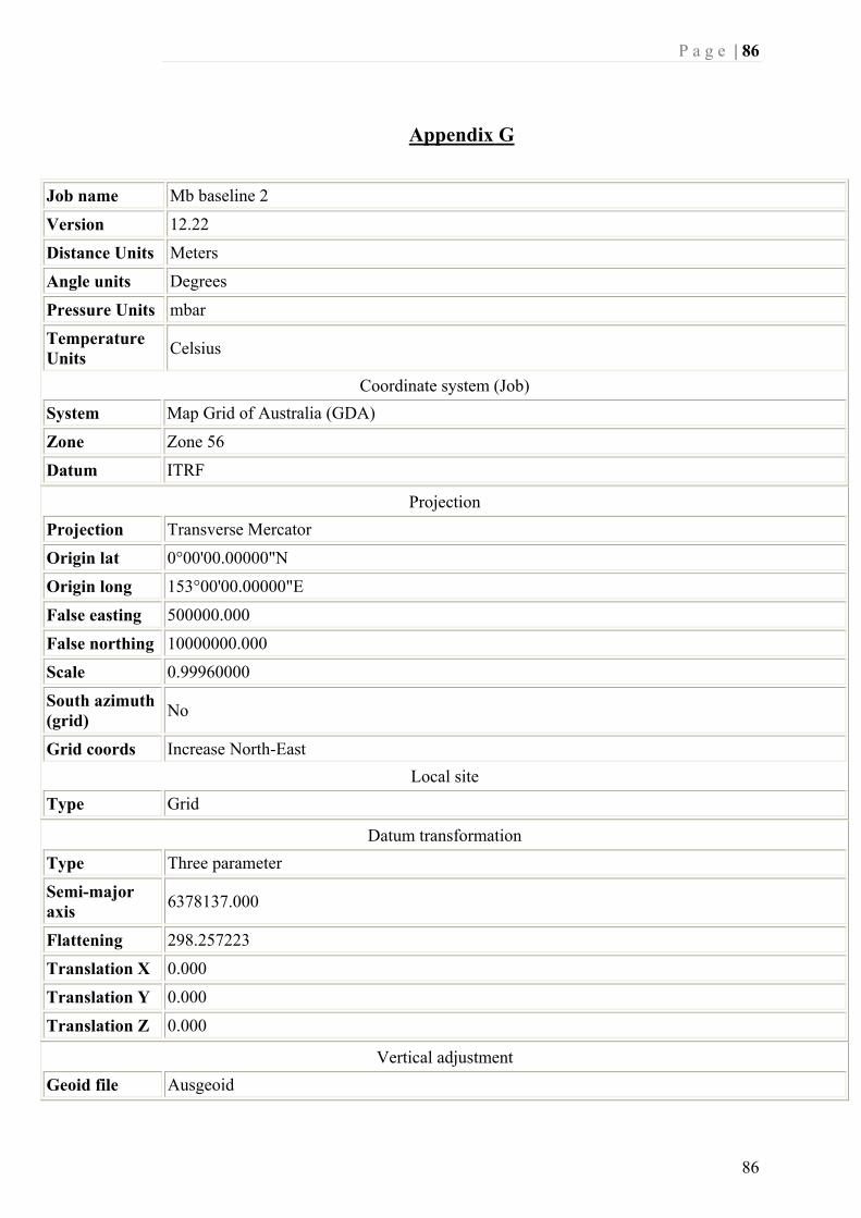
P a g e | 86
86
Appendix G
Job name Mb baseline 2
Version 12.22
Distance Units Meters
Angle units Degrees
Pressure Units mbar
Temperature Units Celsius
Coordinate system (Job) System Map Grid of Australia (GDA)
Zone Zone 56
Datum ITRF
Projection Projection Transverse Mercator
Origin lat 0°00'00.00000"N
Origin long 153°00'00.00000"E
False easting 500000.000
False northing 10000000.000
Scale 0.99960000
South azimuth (grid) No
Grid coords Increase North-East Local site
Type Grid
Datum transformation Type Three parameter
Semi-major axis 6378137.000
Flattening 298.257223
Translation X 0.000
Translation Y 0.000
Translation Z 0.000
Vertical adjustment Geoid file Ausgeoid

P a g e | 87
87
Collected Field Data
Corrections South azimuth (grid) No
Grid coords Increase North-East
Magnetic declination 0°00'00"
Distances Ground
Neighborhood adjustment Off
Projection Projection Transverse Mercator
Origin lat 0°00'00.00000"N
Origin long 153°00'00.00000"E
False easting 500000.000
False northing 10000000.000
Scale 0.99960000 Local site
Type Grid
Datum transformation Type Three parameter
Semi-major axis 6378137.000
Flattening 298.257223
Translation X 0.000
Translation Y 0.000
Translation Z 0.000
Vertical adjustment Geoid file Ausgeoid
Coordinate system System Map Grid of Australia (GDA)
Zone Zone 56
Datum ITRF Rover options
Elevation mask 10 PDOP
mask 6
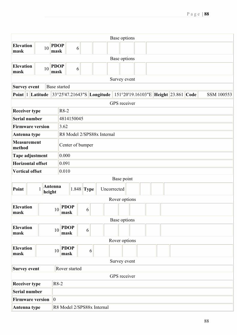
P a g e | 88
88
Base options Elevation mask 10 PDOP
mask 6 Base options
Elevation mask 10 PDOP
mask 6 Survey event
Survey event Base started
Point 1 Latitude 33°25'47.21643"S Longitude 151°20'19.16103"E Height 23.861 Code SSM 100553
GPS receiver Receiver type R8-2
Serial number 4814150045
Firmware version 3.62
Antenna type R8 Model 2/SPS88x Internal
Measurement method Center of bumper
Tape adjustment 0.000
Horizontal offset 0.091
Vertical offset 0.010 Base point
Point 1 Antenna height 1.848 Type Uncorrected
Rover options Elevation mask 10 PDOP
mask 6 Base options
Elevation mask 10 PDOP
mask 6 Rover options
Elevation mask 10 PDOP
mask 6 Survey event
Survey event Rover started GPS receiver
Receiver type R8-2
Serial number
Firmware version 0
Antenna type R8 Model 2/SPS88x Internal

P a g e | 89
89
Measurement method Antenna Phase Center
Tape adjustment 0.000
Horizontal offset 0.000
Vertical offset 0.000 Base point
Point 1 Antenna height 1.855 Type Corrected
Initialization event: Gained
GPS week 1500 Seconds 98150 Initialization
type
On the fly
Survey type
Real-time
Initialization count 3
GPS receiver Receiver type R8-2
Serial number 4803143857
Firmware version 3.62
Antenna type R8 Model 2/SPS88x Internal
Measurement method Center of bumper
Tape adjustment 0.000
Horizontal offset 0.091
Vertical offset 0.010
Point 2 ∆X 7.224 ∆Y -31.142 ∆Z -31.790 Code ch172
Antenna height 1.685 Type Uncorrected Hz Prec 0.003 Vt
Prec 0.006 QC 1 Satellites 9 PDOP 1.2 HDOP 0.4 VDOP 1.1
RMS 8.815 Positions used 186
Std. Dev (H)
? Std. Dev (V)
?
QC 2 Satellites 9 VCV xx (m²) 0.000019
VCV xy (m²)
-0.000016
VCV xz (m²)
0.000012
Error scale (m) 0.010
VCV yy (m²)
0.000016 VCV yz (m²)
-0.000011
VCV zz 0.000011

P a g e | 90
90
(m²)
Point 3 ∆X 20.769 ∆Y -65.631 ∆Z -75.123 Code ch115
Antenna height 1.710 Type Uncorrected Hz Prec 0.002 Vt
Prec 0.006
QC 1 Satellites 9 PDOP 1.2 HDOP 0.4 VDOP 1.2
RMS 9.377 Positions used 185
Std. Dev (H)
? Std. Dev (V)
?
QC 2 Satellites 9 VCV xx (m²) 0.000019
VCV xy (m²)
-0.000015
VCV xz (m²)
0.000013
Error scale (m) 0.010
VCV yy (m²)
0.000015 VCV yz (m²)
-0.000012
VCV zz (m²) 0.000012
Point 4 ∆X 30.358 ∆Y -89.853 ∆Z -105.429 Code ch75
Antenna height 1.673 Type Uncorrected Hz Prec 0.003 Vt
Prec 0.008
QC 1 Satellites 9 PDOP 1.3 HDOP 0.4 VDOP 1.2
RMS 12.978 Positions used 195
Std. Dev (H)
? Std. Dev (V)
?
QC 2 Satellites 10 VCV xx (m²) 0.000028
VCV xy (m²)
-0.000023
VCV xz (m²)
0.000021
Error scale (m) 0.010
VCV yy (m²)
0.000023 VCV yz (m²)
-0.000018
VCV zz (m²) 0.000020
Point 5 ∆X 36.353 ∆Y -105.021 ∆Z -124.420 Code ch50
Antenna height 1.700 Type Uncorrected Hz Prec 0.003 Vt
Prec 0.007 QC 1 Satellites 10 PDOP 1.2 HDOP 0.4 VDOP 1.2
RMS 14.151 Positions used 189
Std. Dev (H)
? Std. Dev (V)
?
QC 2 Satellites 10 VCV xx (m²) 0.000023
VCV xy (m²)
-0.000018
VCV xz (m²)
0.000017

P a g e | 91
91
Error scale (m) 0.010
VCV yy (m²)
0.000017 VCV yz (m²)
-0.000014
VCV zz (m²) 0.000017
Point 6 ∆X 42.314 ∆Y -120.149 ∆Z -143.426 Code ch25
Antenna height 1.700 Type Uncorrected Hz Prec 0.003 Vt
Prec 0.009
QC 1 Satellites 9 PDOP 1.2 HDOP 0.4 VDOP 1.2
RMS 13.114 Positions used 185
Std. Dev (H)
? Std. Dev (V)
?
QC 2 Satellites 9 VCV xx (m²) 0.000033
VCV xy (m²)
-0.000024
VCV xz (m²)
0.000026
Error scale (m) 0.010
VCV yy (m²)
0.000023 VCV yz (m²)
-0.000021
VCV zz (m²) 0.000028
Point 7 ∆X 48.193 ∆Y -135.245 ∆Z -162.438 Code sum 100552
Antenna height 1.720 Type Uncorrected Hz Prec 0.002 Vt
Prec 0.006
QC 1 Satellites 10 PDOP 1.1 HDOP 0.4 VDOP 1.0
RMS 16.189 Positions used 208
Std. Dev (H)
? Std. Dev (V)
?
QC 2 Satellites 10 VCV xx (m²) 0.000014
VCV xy (m²)
-0.000010
VCV xz (m²)
0.000011
Error scale (m) 0.010
VCV yy (m²)
0.000010 VCV yz (m²)
-0.000009
VCV zz (m²) 0.000013
Survey event Survey event End survey
Survey Controller Reduced Points
Point 1 East 345552.377 North 6299831.895 Elevation -0.522 Code SSM 100553
Point 2 East 345576.844 North 6299794.034 Elevation -0.600 Code ch172

P a g e | 92
92
Point 3 East 345601.433 North 6299742.601 Elevation -0.474 Code ch115
Point 4 East 345618.664 North 6299706.547 Elevation -0.457 Code ch75
Point 5 East 345629.459 North 6299683.964 Elevation -0.482 Code ch50
Point 6 East 345640.235 North 6299661.395 Elevation -0.430 Code ch25
Point 7 East 345651.022 North 6299638.869 Elevation -0.323 Code SSM 100552
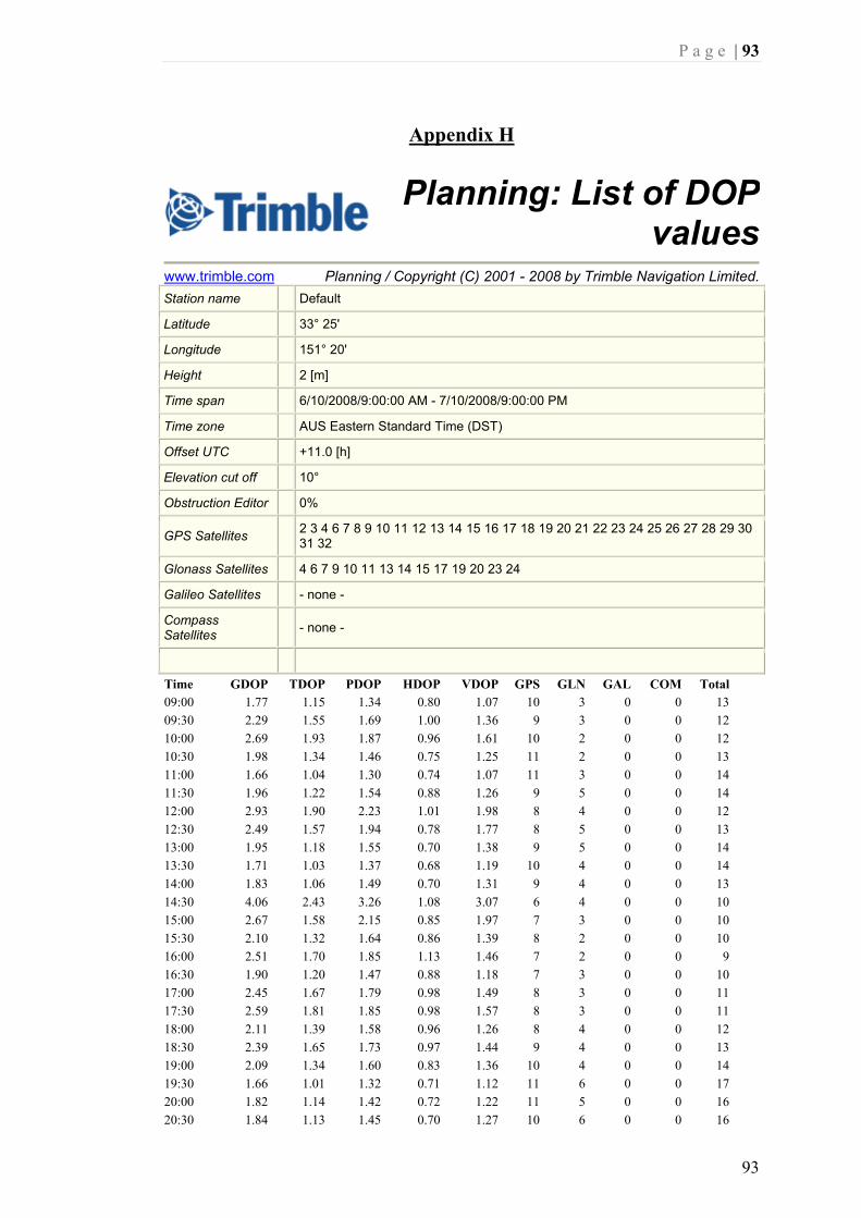
P a g e | 93
93
Appendix H
Planning: List of DOP values
www.trimble.com Planning / Copyright (C) 2001 - 2008 by Trimble Navigation Limited.Station name Default
Latitude 33° 25'
Longitude 151° 20'
Height 2 [m]
Time span 6/10/2008/9:00:00 AM - 7/10/2008/9:00:00 PM
Time zone AUS Eastern Standard Time (DST)
Offset UTC +11.0 [h]
Elevation cut off 10°
Obstruction Editor 0%
GPS Satellites 2 3 4 6 7 8 9 10 11 12 13 14 15 16 17 18 19 20 21 22 23 24 25 26 27 28 29 30 31 32
Glonass Satellites 4 6 7 9 10 11 13 14 15 17 19 20 23 24
Galileo Satellites - none -
Compass Satellites - none -
Time GDOP TDOP PDOP HDOP VDOP GPS GLN GAL COM Total09:00 1.77 1.15 1.34 0.80 1.07 10 3 0 0 13 09:30 2.29 1.55 1.69 1.00 1.36 9 3 0 0 12 10:00 2.69 1.93 1.87 0.96 1.61 10 2 0 0 12 10:30 1.98 1.34 1.46 0.75 1.25 11 2 0 0 13 11:00 1.66 1.04 1.30 0.74 1.07 11 3 0 0 14 11:30 1.96 1.22 1.54 0.88 1.26 9 5 0 0 14 12:00 2.93 1.90 2.23 1.01 1.98 8 4 0 0 12 12:30 2.49 1.57 1.94 0.78 1.77 8 5 0 0 13 13:00 1.95 1.18 1.55 0.70 1.38 9 5 0 0 14 13:30 1.71 1.03 1.37 0.68 1.19 10 4 0 0 14 14:00 1.83 1.06 1.49 0.70 1.31 9 4 0 0 13 14:30 4.06 2.43 3.26 1.08 3.07 6 4 0 0 10 15:00 2.67 1.58 2.15 0.85 1.97 7 3 0 0 10 15:30 2.10 1.32 1.64 0.86 1.39 8 2 0 0 10 16:00 2.51 1.70 1.85 1.13 1.46 7 2 0 0 9 16:30 1.90 1.20 1.47 0.88 1.18 7 3 0 0 10 17:00 2.45 1.67 1.79 0.98 1.49 8 3 0 0 11 17:30 2.59 1.81 1.85 0.98 1.57 8 3 0 0 11 18:00 2.11 1.39 1.58 0.96 1.26 8 4 0 0 12 18:30 2.39 1.65 1.73 0.97 1.44 9 4 0 0 13 19:00 2.09 1.34 1.60 0.83 1.36 10 4 0 0 14 19:30 1.66 1.01 1.32 0.71 1.12 11 6 0 0 17 20:00 1.82 1.14 1.42 0.72 1.22 11 5 0 0 16 20:30 1.84 1.13 1.45 0.70 1.27 10 6 0 0 16

P a g e | 94
94
21:00 1.66 1.01 1.32 0.65 1.15 11 6 0 0 17 21:30 1.85 1.19 1.41 0.76 1.19 11 5 0 0 16 22:00 1.90 1.22 1.46 0.78 1.23 10 4 0 0 14 22:30 1.65 0.96 1.34 0.66 1.16 11 5 0 0 16 23:00 1.70 0.97 1.39 0.62 1.24 11 6 0 0 17 23:30 2.27 1.43 1.77 0.84 1.56 9 4 0 0 13 00:00 2.34 1.48 1.80 1.08 1.44 9 3 0 0 12 00:30 2.39 1.61 1.76 0.96 1.48 8 3 0 0 11 01:00 1.91 1.26 1.45 0.84 1.18 8 4 0 0 12 01:30 2.32 1.60 1.69 0.82 1.47 8 4 0 0 12 02:00 3.00 2.06 2.18 0.89 1.99 8 4 0 0 12 02:30 2.06 1.34 1.56 0.81 1.34 8 5 0 0 13 03:00 2.52 1.67 1.88 0.91 1.65 6 5 0 0 11 03:30 2.46 1.60 1.87 0.95 1.61 6 5 0 0 11 04:00 3.25 2.15 2.43 1.17 2.13 5 4 0 0 9 04:30 1.69 1.06 1.32 0.72 1.11 9 4 0 0 13 05:00 2.16 1.36 1.68 0.80 1.48 8 4 0 0 12 05:30 2.16 1.35 1.68 0.82 1.46 8 4 0 0 12 06:00 3.09 2.02 2.34 1.06 2.09 6 4 0 0 10 06:30 2.76 1.83 2.06 1.05 1.77 7 3 0 0 10 07:00 2.38 1.57 1.80 1.01 1.49 7 4 0 0 11 07:30 1.63 0.98 1.31 0.78 1.04 10 4 0 0 14 08:00 2.86 1.85 2.18 1.06 1.91 9 2 0 0 11 08:30 2.53 1.76 1.81 0.87 1.59 9 2 0 0 11 09:00 1.79 1.16 1.36 0.82 1.09 10 3 0 0 13 09:30 2.32 1.57 1.71 1.00 1.38 9 3 0 0 12 10:00 2.62 1.88 1.82 0.91 1.58 10 2 0 0 12 10:30 2.10 1.49 1.47 0.73 1.28 11 2 0 0 13 11:00 1.72 1.12 1.30 0.71 1.10 11 3 0 0 14 11:30 1.89 1.16 1.49 0.78 1.26 9 5 0 0 14 12:00 2.13 1.33 1.66 0.78 1.47 8 5 0 0 13 12:30 3.01 1.96 2.28 0.97 2.07 8 3 0 0 11 13:00 2.35 1.42 1.86 0.93 1.61 9 3 0 0 12 13:30 1.89 1.11 1.53 0.72 1.35 9 3 0 0 12 14:00 2.33 1.51 1.78 0.83 1.58 9 2 0 0 11 14:30 3.08 1.85 2.46 1.02 2.24 6 4 0 0 10 15:00 2.30 1.43 1.80 0.89 1.56 7 4 0 0 11 15:30 2.14 1.41 1.60 0.87 1.35 8 3 0 0 11 16:00 2.19 1.40 1.69 0.90 1.42 7 4 0 0 11 16:30 2.33 1.51 1.77 0.96 1.48 7 4 0 0 11 17:00 2.09 1.38 1.57 0.93 1.26 8 4 0 0 12 17:30 1.93 1.26 1.46 0.94 1.12 8 4 0 0 12 18:00 2.65 1.85 1.89 0.99 1.61 8 3 0 0 11 18:30 2.27 1.51 1.70 0.91 1.44 9 4 0 0 13 19:00 2.13 1.33 1.67 0.76 1.48 10 4 0 0 14 19:30 1.90 1.12 1.54 0.73 1.36 12 5 0 0 17 20:00 1.90 1.18 1.49 0.81 1.25 11 4 0 0 15 20:30 1.80 1.06 1.46 0.85 1.19 10 5 0 0 15
21:00 1.85 1.16 1.44 0.74 1.23 11 5 0 0
16
Page 1/1

P a g e | 95
95
Appendix I

P a g e | 96
96

P a g e | 97
97

P a g e | 98
98
Appendix J

P a g e | 99
99

P a g e | 100
100
Appendix K

P a g e | 101
101
Appendix L

P a g e | 102
102

P a g e | 103
103