Investigation of Vortex Generators for Augmentation … • UC Category 1210 • DE97000087 Investigation of V o Generators for Au of Wind Turbine Performance X entation …

NREL/SR-440-21399 • UC Category 1210 • DE97000087

Investigation of V o Generators for Au of Wind Turbine Performance

X entation er

Dayton A. Griffm

R. Lynette & Associates, Inc.

Seattle, Washington

NREL technical monitor: Paul Migliore

National Renewable Energy Laboratory 161 7 Cole Boulevard Golden, Colorado 80401-3393 A national laboratory ofthe U.S. Department ofEnergy Managed by Midwest Research Institute for the U.S. Department of Energy under contract No. DE-AC36-83CH1 0093

Work prepared under Subcontract No. ZAA-5-12272-05

December 1996

NOTICE This report was prepared as an account of work sponsored by an agency of the United States government. Neither the United States government nor any agency thereof, nor any of their employees, makes any warranty, express or implied, or assumes any legal liability or responsibility for the accuracy, completeness, or usefulness of any information, apparatus, product, or process disclosed, or represents that its use would not infringe privately owned rights. Reference herein to any specific commercial product, process, or service by trade name, trademark, manufacturer, or otherwise does not necessarily constitute or imply its endorsement, recommendation, or favoring by the United States government or any agency thereof. The views and opinions of authors expressed herein do not necessarily state or reflect those of the United States government or any agency thereof.

*''

Available to DOE and DOE contractors from: Office of Scientific and Technical Information (OSTI) P.O. Box 62

Oak Ridge, TN 3783 1 Prices available by calling ( 423) 57 6-8 40 1

Available to the public from: National Technical Information Service ( NTIS) U.S. D epartment of Commerce

5285 Port Royal Road Springfield, VA 22 1 61 (703) 487- 4650

'•-' Printed on paper containing at least 50% wastepaper, including 20% postconsumer waste

FOREWORD The National Renewable Energy Laboratory's (NREL' s) National Wind Technology Center is supporting the efforts of its industry partners to develop advanced, utility-scale wind turbines. Part of the research being conducted focuses on innovative components and subsystems that eventually may be incorporated into these advanced turbines. R. Lynette & Associates chose to investigate, among other technologies, the use of vortex generators to enhance power performance and annual energy capture of wind turbine rotors.

The application of vortex generators to wind turbine blades has been investigated previously, with mixed success. When the present study was initiated, there existed considerable uncertainty regarding its

·potential outcome. However, the modest objective of increasing energy capture by 1% to 3% seemed possible, and the proposed investigative approach was expected to yield considerable insight and to contribute significantly to the aerodynamic literature.

The author and his colleagues at R. Lynette & Associates are commended for the formulation and execution of a meticulous analysis that embodied all the classical elements of scientific

investigation-hypothesis, literature search, laboratory tests, data analysis, design, fabrication and field testing-all executed with precision and scrupulous attention to detail.

NREL and the U.S. Department of Energy are proud to support research activities of the high quality represented by this project and documented in this report.

iaul G. Migifofej>h.D. NREL Senior Project Manager

lll

PREFACE

The present work was supported by NREL, under Subcontract #ZAA-5-12272-05, monitored by Paul Migliore. The author would like to thank Paul and others at NREL for their support on this project, including many helpful technical discussions. The large number of configurations tested in the wind tunnel, and the quality of the data, formed a solid foundation for this work. The success of the wind tunnel test was due to the effort of Professors David Russell and Scott Eberhardt, the design assistance of Bob Blair, the machining support of Bill Lowe, and the outstanding work performed by the entire crew of University of Washington Aeronautical Laboratory (UW AL). Paul Robertson and his engineering staff at Aeronautical Testing Services were invaluable in manufacturing the wind-tunnel models, and providing both materials and advice for the wind-tunnel and field tests. Thanks also to Shawn Lawlor and Richard Beckett, who both contributed much inspiration and insight to this project.

iv

ABSTRACT

This study focuses on the use of vortex generators (VGs) for performance augmentation of the stallregulated A WT -26 wind turbine. The goal was to design a VG array which would increase annual energy production (AEP) by increasing power output at moderate wind speeds, without adversely affecting the loads or stall-regulation performance of the turbine.

Wind tunnel experiments were conducted at the University of Washington to evaluate the effect of VGs on the AWT-26 blade, which is lofted from National Renewable Energy Laboratory (NREL) S-series airfoils. Based on wind-tunnel results and analysis, a VG array was designed and then tested on the AWT-26 prototype, designated Pl. Performance and loads data were measured for Pl, both with and without VGs installed. The turbine performance with VGs met most of the design requirements; power output was increased af moderate wind speeds with a negligible effect on peak power. However, VG drag penalties caused a loss in power output for low wind speeds, such that performance with VGs resulted in a net decrease in AEP for sites having annual average wind speeds up to 8.5 m/s.

While the present work did not lead to improved AEP for the A WT -26 turbine, it does provide insight into performance augmentation of wind turbines with VGs. The safe design of a VG array for a stallregulated turbine has been demonstrated, and several issues involving optimal performance with VGs have been identified and addressed.

v

TABLE OF CONTENTS

1.0 INTRODUCTION ........................................................................................... 1-1 1.1 Background ............................................................................................ 1-1 1.2 Project Schedule ...................................................................................... 1-1 1.3 Purpose ..... ... . . .. . .............................................................. .. ..... .. .. . . . ... . . . . . 1-1 1.4 Objectives ............................................................................................. 1-2 1.5 Approach .............................................................................................. 1-2

2.0 VORTEX GENERA TOR AERODYNAMICS ................................•... . .................... 2-1 2.1 VG Array Parameters ............................................................................... 2-1 2.2 Wind Turbine Applications ........................................................................ 2-1

3.0 WIND TUNNEL EXPERIMENTS ...................................................................... 3-1 3.1 UWAL Tunnel. ....................................................................................... 3-1

3.1.1 2-D Test Section ........................................................................ 3-1 3.1.2 Flow Quality and Calibration ......................................................... 3-1 3.1.3 Data Acquisition and Reduction ...................................................... 3-2

3.2 Test Matrix ............................................................................................ 3-5 3.3 Wind Tunnel Test Results and Discussion ...................................................... 3-7

3.3.1 Tare Drag Measurements .............................................................. 3-7 3.3.2 Baseline Airfoils ......................................................................... 3-7 3.3.3 Co-Rotating VG Performance ........................................................ 3-13 3.3.4 Counter-Rotating VG Performance .................................................. 3-13 3.3.5 Effect of Leading Edge Roughness .................................................. 3-21 3.4.6 Reynolds Number Effects ............................................................. 3-21 3.3.7 VG Yaw Sensitivity .................................................................... 3-21 3.3.8 Summary of Results .................................................................... 3-27

4.0 DESIGN AND ANALYSIS .... .......................................... ..... . . ....... . ... ............... 4-1 4.1 Scaling of Wind-Tunnel Test Data ........................................................... .4-1 4.2 Constraints I Design Space ...................................................................... 4-2 4.3 Performance Trades Using PROPPC ......................................................... A-2 4.4 Designing for Smooth Stall Progression ..................................................... A-4 4.5 VG Configuration #1 ............................................................................. 4-5

5.0 FULL-SCALE PERFORMANCE TEST ............................................................... .S-1 5.1 Baseline Turbine Description ................................................................... 5-1 5.2 Data Acquisition and Analysis ................................................................. 5-l 5.3 P1 Baseline Performance ........................................................................ S-5 5.4 P1 with VG Configuration #1 ................................................................. .S-9

5.4.1 Effect on Power Curve ................................................................. 5-9 5.4.2 Effect on Loads .......................................................................... S-12 5.4 .3 Analysis I Suggested Improvements to Configuration .......................... .5-17

6.0 RESULTS AND CONCLUSIONS ....................................................................... 6-1

7.0 REFERENCES ............................................................................................... 7-1

vi

Figure

2-1 2-2 2-3 3-1 3-2 3-3 3-4 3-5 3-6 3-7 3-8 3-9 3-10 3-11 3-12 3-13 3-14 3-15 3-16 4-1 4-2 5-1 5-2 5-3 5-4 5-5 5-6 5-7 5-8 5-9 5-10 5-11 5-12 5-13

LIST OF FIGURES

Page

Schematic of Counter- and Co-Rotational VG Arrays ........................................... 2-1 Parameters which Define Vortex-Generator Configurations .................................... 2-3 Regions of VG Effect on Airfoil Lift Curve ........................................ . .............. 2-5 Two Dimensional Test Section at UW AL .......................................................... 3-2 Nominal Test Matrix for VG Wind Tunnel Test .................... ..................... . ........ 3-6 Repeatability of Lift and Drag Measurements for AWT-2601 Model ............. ........... 3-8 Comparison of UWAL AWT-2601 with OSU Data and Eppler Calculations .......... . .... 3-10 Baseline Lift and Drag Curves for A WT Models .......................... �·-····················3-11 Baseline Moment Curves for A WT Models ........ . . ............................................. 3-12 Variation of VG Effectiveness with Chord wise Placement ................... ................. .3-14 Variation of VG Effectiveness with Height ............................. . .......................... 3-15 Variation of VG Effectiveness with Array Density .............................................. 3-16 Impact of Array Density on VG Drag Penalty .......................... . . . ....................... 3-17 Comparison of Co-Rotating and Counter-Rotating VG Arrays ................................ 3-19 Pair Spacing Study for Counter-Rotating VGs . .................. . . ............................... 3-20 Effect of Leading-Edge Roughness .................................................................. 3-23 Reynolds Number Effect on Clean Airfoil ......................................................... 3-24 Reynolds Number Effect on VG Performance ..................................................... 3-25 Effect of Yaw on VG Performance .... ......... . .................................................... 3-26 Vortex Generator Design Space for A WT-26 Rotor Blade .................................... .4-3 VG Configuration #1 Installed on P1 Rotor Blade ..................................... ... ...... .4-7 Prototype Turbines at A WT Tehachapi Test Site ................................................. 5-1 General Location of A WT Tehachapi Test Site .................... .............................. .5-2 Plot Plan of Pl Test Site ..................................................................... ......... .5-4 Power Curve Data, P1 Baseline Performance Test ............................................. . . 5-6 Repeatability of Pl Baseline Power Curve, 50 Hour Data Sets ................................ 5-7 Repeatability of P1 Baseline Power Curve, 300 Hour Data Sets .............................. 5-8 Repeatability of P1 Power Curve with VGs, 300 Hour Data Sets ..... . . . . .................... 5-10 Effect of VG Configuration #1 on Pl Performance ......... . . . . .................... ............. 5-11 10-Minute Average Wind Speeds during P1 Loads Measurement ............................. 5-13 Nacelle Pitch Accelerations, Full Data Sets ........................................ . .............. 5-15 Nacelle Pitch Accelerations, Wind Speeds between 8.9 and 15.6 rn/s . ..................... .5-15 P1 Generator Output, Rainflow Cycle Counts ............................................. . . . .... 5-16 P1 Tower Leg Axial Loads, Rainflow Cycle Counts ............................................ 5-16

vii

Table

1-1 3-1 3-2 3-3 3-4 4-1 4-2 5-1 5-2 5-3

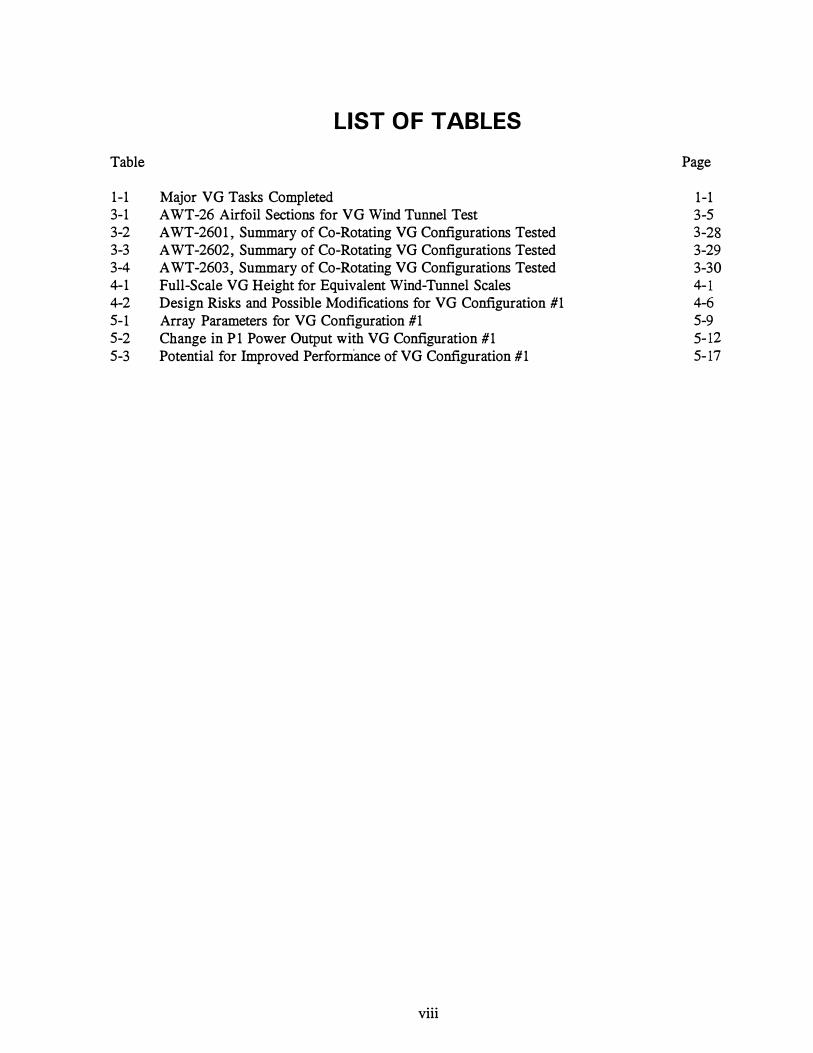
LIST OF TABLES

Major VG Tasks Completed A WT -26 Airfoil Sections for VG Wind Tunnel Test AWT-2601, Summary of Co-Rotating VG Configurations Tested A WT-2602, Summary of Co-Rotating VG Configurations Tested A WT-2603, Summary of Co-Rotating VG Configurations Tested Full-Scale VG Height for Equivalent Wind-Tunnel Scales Design Risks and Possible Modifications for VG Configuration #1 Array Parameters for VG Configuration #1 Change in P1 Power Output with VG Configuration #1 Potential for Improved Performance of VG Configuration #1

viii

Page

1-1 3-5 3-28 3-29 3-30 4-1 4-6 5-9 5-12 5-17

ADAS AEP AWT c em COE d D ft h HAWT in kV kW 1 lbs m MET mm mph MW N NACA NREL Pa PC PCM PLC. psf RLA R Re rpm. SERI sow sps VG X

ABBREVIATIONS

Advanced Data Acquisition System Annual energy production Advanced Wind Turbines Airfoil chord Centimeter/centimeters Cost of energy Lateral spacing between two vortex generators Lateral spacing between two vortex generator pairs Feet/foot Vortex generator height Horizontal axis wind turbine Inch/inches Kilovolt Kilowatt Vortex generator length Pounds force Meter/meters Meteorological (tower) Millimeter/millimeters Miles per hour Megawatt Newton/Newtons National Advisory Committee for Aeronautics National Renewable Energy Laboratory Pascals Personal computer Power curve monitor Programmable logic controller pounds per square foot R. Lynette & Associates Radial position along turbine blade Reynolds Number Revolutions per minute Solar Energy Research Institute Statement of work Samples per second Vortex Generator Distance from airfoil leading edge, measured parallel to chord-line

ix

CD CL CLmax eM Pmax a.vG

CJ.vG,stall

p

Po

LIST OF SYMBOLS

Drag coefficient (defined in Section 3.1.2) Lift coefficient (defined in Section 3.1.2) Maximum value of lift coefficient Moment coefficient (defined in Section 3 .1.2) Maximum turbine generator power

VG angle of attack, relative to airfoil chord line

Airfoil angle of attack at which VGs become stalled

Air density

Sea-level air density (1.225 kg/m3)

X

1 .0 Introduction

1 . 1 Background

The R. Lynette & Associates (RLA) Next-Generation Innovative Subsystems (NGIS) program is designed to develop innovative subsystems which can be used to improve the performance and cost effectiveness of the A WT-26 wind turbine and which may be usable on other advanced wind turbine designs. RLA is working cooperatively with the National Renewable Energy Laboratory (NREL) and Advanced Wind Turbines Incorporated (A WT) on the program. The program includes a thorough examination of the use of vortex generators (VGs) to improve the performance of the A WT-26 turbine.

1 .2 Project Schedule

Table 1-1 summarizes the major VG Tasks of the Innovative Subsystems Project and compares the original schedule with actual completion dates. The majority of the project was completed between two and four months later than scheduled. The start of the VG Field Test was substantially delayed due to prioritization of site resources towards the installation of the A WT -27 prototype, P4. As a result, the Field Test was started near the end of the Tehachapi wind season, and additional weeks of testing were required to collect sufficient performance data. Originally, field-testing was planned for a second VG configuration. However, due to the disappointing performance results from the first configuration, testing of the second configuration was canceled. No new work was done on the VG project between the termination of the field testing and the completion of the Draft Report.

Table 1 -1 . Major VG Tasks Completed

Innovative Subsystems Completion Dates Task Ori2inal Project Schedule Actual

2. 1 .3 Wind Tunnel Testing 02/28/95 04/14/95

2. 1 .4 Design Full-Scale Configuration 05/07/95 07/13/95

5 . 1 . 1 VG Field Test Plan 05104195 08/01/95

5.3 . 1 VG Test Readiness Review 06/23/95 09/07/95 5.4.3 Establish P1 Baseline Data 04/14/95 05/18/95

5 .4.4 Install VGs on P1 Turbine 06/23/95 09/07/95

5 .4.6 Analyze Field Test Results . 08/01/95 12/18/95

2.4. 1 Draft VG Report 1 1/23/95 06/07/95

2.4.2 Final VG Report 01112/96 10/18/96

1.3 Purpose

This report summarizes all significant work performed on the Vortex Generators Project. It documents the wind-tunnel testing, the design process for the selected VG configuration and the methods, results, and conclusions from the field testing of VGs.

1- 1

1 .4 Objectives

The objectives of this project were to:

1 . Identify a VG configuration that best augments the performance of A WT turbines, without adversely effecting the turbine dynamics or stall behavior.

2. Gain a greater understanding of the effect of VGs on NREL airfoils, and insight into how VGs may be of use in performance augmentation for a broader class of wind turbines.

1 . 5 Approach

A literature search was conducted of previously reported work with VGs, and in particular, V:G applications to wind turbines. Wind tunnel tests were designed to evaluate the effect of VGs on the aerodynamic performance of airfoil sections which are characteristic of the A WT-26 turbine blades. The wind tunnel results, along with insights gained through the literature search, then formed a database from which to design a VG configuration for full-scale testing. The analytic computer code PROPPC [1] was used, with wind tunnel data, to conduct performance trade studies for VG sizing and placement, and the effects of various constraints on the design were investigated.

A VG configuration was selected for testing on the AWT-26 prototype, P l . As part of the field test, careful measurements were made of the baseline P1 power curve and loads. VG Configuration #1 was then installed on P 1 , and power curve and loads were again measured. Based on analysis of the test results, it was decided not to test a second VG configuration on P l .

1-2

2.0 Vortex Generator Aerodynamics

Vortex generators are typically small wing-like devices which protrude from an aerodynamic surface. The VGs are oriented so they produce streamwise vortices, which enhance mixing between the freestream air and the local boundary layer, thinning and energizing the boundary layer so that it can withstand higher adverse pressure gradients prior to flow separation. When used on an airfoil, VGs delay the onset of stall, increase the maximum lift coefficient, and result in some drag penalty at low airfoil angles of attack.

2. 1 VG Array Parameters

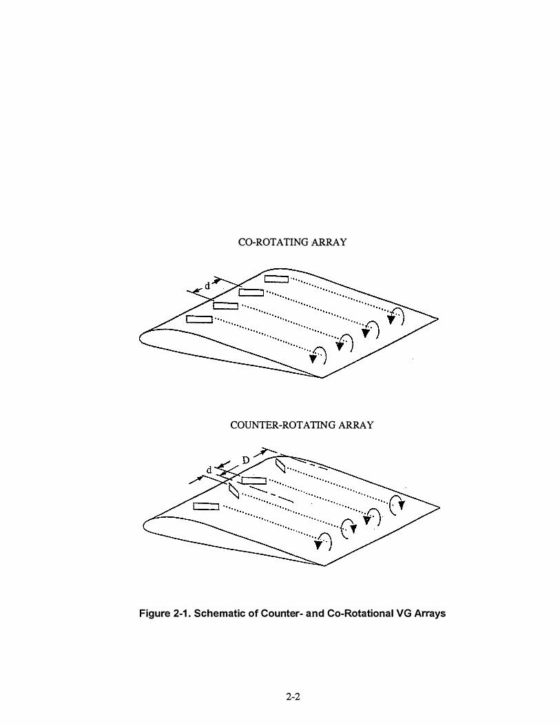
VG configurations are of two basic types: co-rotating and counter-rotating arrays. Figure 2-1 shows airfoils with both array types, with arrows indicating the sense of rotation of the resulting vortices. The co-rotating array produces vortices with the same sense of rotation, while the counter-rotating array produces vortex pairs with lateral regions of common-flow up and common-flow down. Note that a co-rotating array has a single lateral spacing parameter, d, while the counter-rotating array has two lateral spacing parameters, d = distance between two VGs which form a pair and D = distance between each pair of VGs.

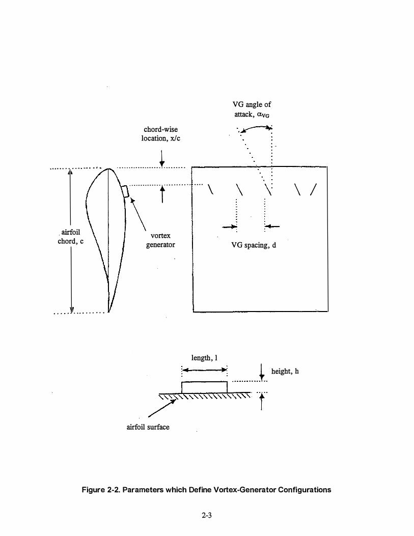
Additional VG parameters are illustrated in Figure 2-2, where VGs of the flat-vane type are shown again. For this type of VG, a configuration will be completely defined by the parameters shown. Note that all of the spacing parameters may be given in physical dimensions, but will frequently be normalized to another characteristic dimension (e.g., x/c, h/c, diD).

2.2 Wind Turbine Applications

The first reported use of VGs to improve wind turbine performance was in 1983, when counterrotational VG arrays were installed on the horizontal axis wind turbine (HAWT) Boeing MOD-2 [2]. The MOD-2 blades used a family of National Advisory Committee for Aeronautics (NACA) 230XX airfoils which are known to be sensitive to roughness effects and were generally operated with rough surface-finish condition. The MOD-2 blade aerodynamics were far from optimal and so the use of VGs resulted in a large (1 1 %-15% ) increase in AEP for the turbine.

The. MOD-2 results were scaled to design a vortex generator configuration for the Carter Model 25, resulting in a 20% increase in peak power output and an estimated 8 % increase in revenue at an 8 m/s (18 mph) average wind-speed site [3] . Although a similar gain in performance could be achieved by pitching the turbine blades to low angles of attack (feather), the vortex generators offered the additional advantage of decreased sensitivity to roughness [3].

In 1988, a successful application of VGs on a 50 kW DAF two-bladed Darrieus vertical axis wind turbine was reported [4]. Test results showed a 72 % increase in peak power, and predicted a 17% increase in AEP at the test site.

A less successful test was reported in 1990 when VGs were applied to several ESI 54 HAWTs [5]. Although the turbine performance results with VGs were initially encouraging, unstable rotor dynamics destroyed one rotor and the VG test was canceled.

2- 1

CO-ROTATING ARRAY

COUNTER-ROTATING ARRAY

Figure 2-1 . Schematic of Counter- and Co-Rotational VG Arrays

2-2

... .. . . .. "' . . ... ... . .. ..

. airfoil chord, c

. . . . . .... . . . . . . .

chord-wise location, x/c

.................. t ....... . · · ·········•••t ••···· ·· · · .... \

\ vortex

generator

length, 1

VG angle of

attack, avG

VG spacing, d

\ I

=� )llo: � height, h

7 J,,,," "J ��--:r: airfoil surface

Figure 2-2. Parameters which Define Vortex-Generator Configurations

2-3

The early successes of VG applications to wind turbines had several things in common: the airfoils of the turbine blades were NACA sections and the VGs were used to significantly increase the maximum lift coefficient. The advantage of using VGs is much less obvious for a stall-regulated rotor which uses airfoils designed to minimize roughness effects and with low CLmax outboard on the blade. Use of VGs to delay stall and increase CLmax seems contrary to both the rotor and airfoil designs.

The present study was motivated by the idea that VGs may still be used to improve a stall-regulated turbine performance although the margin for improvement is smaller than for early wind turbine designs. With proper sizing and placement, VG arrays may delay stall and increase lift up to a specified wind speed at which the VGs themselves will become stalled, thereby allowing the turbine to retain its baseline post-stall performance. This is illustrated by Figure 2-3, which shows an example of an S815 airfoil lift curve and a possible modification with VGs. Three regions are indicated on the lift curve of Figure 3:

Region A -

Region B -

Region C-

Here the baseline lift curve is already linear. In this region VGs can not increase lift and must cause some drag penalty.

Here VGs delay stall, causing the lift curve to remain linear to a higher angle of attack, and increasing CLmax· The VGs will cause a net decrease in drag in this region, as the form drag of the airfoil is decreased.

Here the airfoil is stalled, and the VGs are embedded in the airfoil wake. In this region the VGs should have no effect on either lift o_r drag of the airfoil.

For VGs to cause a net increase in power production, the lift and drag benefits in region B must outweigh the drag penalty paid in region A. Of additional concern is the increased sharpness of stall in region B. For the case illustrated in Figure 2-3 , the VGs will be of benefit between 6° and 18° angles of attack. The design stall angle is 18°, beyond which the VGs should have no effect. In the present work, the angle of attack beyond which VGs have no effect is designated the VG stall angle, ava,staii· Note that for a specific wind-turbine blade and pitch setting, the VG stall angle would have a corresponding wind speed.

·

In this work, the VG drag penalty of region A will be loosely referred to as the penalty in minimum drag, even though the drag penalties were measured at zero airfoil angle of attack rather than at the minimum drag condition. Drag effects will most commonly be cited in units of 'drag counts,' where each count is an increment of 0.0001in. drag coefficient.

In region B, it is important to distinguish between two effects, linearization of the lift curve and increase in maximum lift coefficient. In Figure 2-3, the lift curve with VGs has been highly linearized up to about 10° angle of attack, and for angles above that the lift curve becomes non-linear. The maximum lift coefficient has been increased to about CLmax = 1. 7. Note that these effects are not identical. Two VG configurations could result in the same CLmax, but one may lead to significantly more linearization of the lift curve.

2-4

1.8 .------.----�------------------�-r----------------� 1.6

1.4

...... 1.2 r::: Cl) ·c:::; 1 :.;:::: -Cl) 8 0.8 ...... !'!:: -I 0.6

0.4

0.2

-5

...--"" : . - \: S815 Data:

----------------- . -.. -------------·-----.--·--. ----------_../._ ----·--.--""\---------------.----.--! t / � \ ! UW AL Wind-Tunnel Test : ;: : \ :

------------·--·- ····--------------�-------·--··f·+----····--·--·---�----\-----·--·--:·--·-- q wall= 1200 Pa : 1 : \ : Re = 1.8 million ; /, : \

------------·--·- ·--·--------------�----·--1- -·-------�-----·--·---------�---.,

----------------- ·----------------

.

-· ----·--·------·:------·--·--·--·---:---------- -·--···r--·-------------·-r · --· -----·------

.

-·--·-- · -- ·- ··1 ------------·--·- ····------- -----+-· -·-----·------+-----····--····--+--------- -·--·-+--·-------------·+·-----·--·-------+----·--·--·--····1

i REGION � � REGION � I - -- - ---------+ - -

B C

---

_, - -1 ------------·-- ��-�-;�-� -·--·---------r··--·--·-----·---r--------- -·--·-1·-·-------------·I·--·--·--·-------r··--·------------l

-------- -·----

A ---·--·-------r-----·--·--·--·---r--------- -·--·-!·--·-------------·-(--·--·--· -------r ----·--·--·--·---

0

. . . . . . . . . 5 10 15 20 25 30

Angle of Attack (degrees) 35

- Measured S815 --·Possible Modification with VGs

Figure 2-3. Reg ions of VG Effect on Airfoil Lift Curve

2-5

3.0 Wind Tunnel Experiments

Wind tunnel experiments were designed to provide VG performance data specific to the NREL airfoil sections that are characteristic of the A WT -26 blade. These experiments were used to determine the extent to which VGs may be of use on the A WT -26 and to develop a database necessary for a full-scale design. Specifically, the experiments were used to quantify the incremental changes in lift and drag for airfoils with VG arrays of varying density, height, orientation and chordwise placement. The wind tunnel tests are summarized in this report and documented in detail in UWAL Repon 1523 [6] .

3 . 1 UWAL Wind Tunnel

The wind-tunnel experiments were conducted in the subsonic, double-return, closed-circuit tunnel at the University of Washington Aeronautical Laboratory (UW AL). The UW AL test section is 2.4 m high x 3 .6 m wide x 3.0 m long (8 x 12 x 10 ft), vented to the atmosphere, with windows on all sides. The tunnel can supply dynamic pressures from 47.8-4780 Pa (1-100 psf) and wind-speeds from 8.9-89 m!s (20-200 mph) with approximately zero flow angularity and 0.72% turbulence intensity.

3. 1. 1 2-D Test Section

A 2-D modification of the 2.4 x 3 .6 m test section was designed and fabricated cooperatively by A WT and UW AL. The 2-D insert was formed by 15.2 em (6 in)-thick walls, which extended from floor to ceiling and approximately 0.3 m (1 ft) forward and 0.9 m (3 ft) aft of the 3-D test section, and were mounted with a lateral separation of 1 .22 m (4 ft) to centers. Airfoils were mounted between two turntables, which were flush with the 2-D walls, and were in turn supported by the UW AL force balance. The balance struts were embedded in the 2-D walls and were not impacted by the airflow through the test section. The mounting apparatus was designed to allow continuous pitch variations between -5° and +45°. Higher angles of attack could be tested by mounting the model at a different angle relative to the turntables. Figure 3-1 shows the 2-D test section with an A WT model mounted.

3.1.2 Flow Quality and Calibration

Total/static pressure ports were installed at four locations to measure the indicated 2-D section dynamic pressure (CI:rwALV· To account for the effects of compressibility, actual dynamic pressure (q� was obtained from the following equation:

<iA = 0.9970*CJrwALL

This calibration incorporated the effect of compressibility as found in a standard dynamic pressure survey of the test section with the 2-D walls installed [7] . A five-hole-probe was used to survey flow angularity in the 2-D section: the average upflow angle (.6-Cl.upflow) of -0.333° was corrected in the data reduction.

Both of the 2-D walls were pressure-tapped along a line 1 .22 m (4 ft) from the floor, and these taps were used to measure the pressure history along the 2-D section walls. The wall pressures were combined with a pressure survey along the tunnel centerline to evaluate the streamwise pressure history in the 2-D section. At the model location, the change in pressure coefficient along the 2-D section was measured as dCp/dl = -0.0164 m·1, and this was used to correct for buoyancy drag effects.

3- 1

During check-out of the 2-D section, yarn tufts were attached to the model and tunnel side walls for flow visualization. The flow around the model appeared very two-dimensional at low angles of attack and fairly steady and symmetric at angles of attack approaching stall.

Figure 3-1. Two Dimensional Test Section at UWAL

3.1.2 Data Acquisition and Reduction

The test models were mounted on the UW AL external balance such that they spanned the distance between the 2-D walls. The standard test run was at constant dynamic pressure and variable angle of attack. Forces were measured with UWAL 's 6-component force and moment balance, which has a maximum capability ofL max = 11,120 N (2500 lbs) and Dmax = 1112 N (250 lbs). The balance components were zeroed at the beginning of each run, with the model set at zero pitch angle, and they were checked for any shift in zero readings at the conclusion of each run. Data reduction included corrections for balance interactions, and the balance calibration was checked twice daily during the test.

3- 2

As mentioned above, a streamwise pressure gradient (dCp/dl) was present in the test section. This change in pressure caused a section drag (®) on the model, given by [7]:

LID- _l:A � dCp � ( )2 - 8 12 dl

qA 12 where A is a factor depending on the shape of the airfoil's base profile, b is the span and c is the chord. The following equation shows how A was calculated:

1

A=� �� (1-Cp)[t+ (:r�:J where x and y are, respectively, the horizontal and vertical coordinates of the airfoil surface as measured from the leading edge along the chord and Cp is the pressure coefficient.

Solid and wake blockage corrections were also applied to the dynamic pressure. Blockage-corrected actual dynamic pressure ( qc) was calculated from the following equation:

sT is the total fractional velocity increment due to blockage:

where ssB and sWB are the solid blockage and wake blockage correction .factors, respectively. The following equations were used for esB and ews:

SsB = Acr c SWB =-Cdu

4h

where h is the test section height, cr is a factor depending on the size of the airfoil relative to the test section, and Cdu is the uncorrected drag coefficient. The following equations show how the constants were calculated:

The proximity of the tunnel walls to the model resulted in a constraint to the flow field, which must be taken into account to obtain approximate free air conditions. Based on the relationships of reference

3-3

8, lift, drag, and moment coefficients and angle of attack were corrected for tunnel upflow and restriction of flow due to the tunnel walls:

The above equations were simplified by ignoring the compressibility corrections within the relationships in reference 8. It is assumed that the dynamic pressure calibration accounts for compressibility and that any additional effects of compressibility are negligible.

The data were reduced to coefficient form and corrected angles of attack were obtained with the following equations:

a c = au + !l.a upflow + !l.a

where Sw is the reference wing area. Moment coefficients are about the quarter chord. The

increments LlCb .6.Cd, LlCm114, and Lla. are the wall corrections applied to the lift, drag, and pitching moment coefficients and angle of attack, respectively.

Semi-corrected plots of lift, drag, and moment data were available on-line during the wind tunnel runs, and fully corrected data were available the following day. On-line plots were used to establish trends during the test, make decisions about the test matrix and to ensure that data was reasonable. Fully corrected data were used to asses detailed performance.

3-4

3.2 Test Matrix

Three airfoil sections, taken from span wise stations along the A WT-26 blade, were selected for the test. The A WT-2601 was a pure NREL S815 with a thickened trailing edge. The A WT-2602 and 2603 were hybrids of S815/S809 and S809/S810 airfoils, respectively.

The wind-tunnel models of these sections, which were 61 em (24 in) long, were machined from rolled aluminum plate by Aeronautical Testing Services in Arlington, W A. With maximum dynamic pressure (q) of 4310 Pa (90 psf), these models allowed testing at Reynolds numbers in excess of Rec=3xl06, which is equal to or higher than the value typical for the full-scale turbine. Table 3-1 summarizes the spanwise sections and scales of the three models which were tested. The calculated Reynolds numbers are at standard sea-level conditions and are based on the rotational velocity of the blade.

Table 3-1. AWT-26 Airfoil Sections for VG Wind-Tunnel Test

Model Name Blade Location Blade Chord Model Scale Blade Full-Scale (% R) (em) Reynolds Number

AWT 2601 35 114.0 0.54 1.9 million AWT-2602 55 99.0 0.61 2.6 million AWT-2603 75 78.4 0.78 2.8 million

A VG planform for testing was selected on the basis of effectiveness, simplicity of manufacture and ease of installation. Based on the literature review, and on insight gained from the Boeing Company and Aeronautical Testing Services, a rectangular planform was selected. For the purpose of the windtunnel test small brass angles were available from a model supply shop in the expected sizes of interest. Although the Boeing Company and Aeronautical Testing Services both put a leading-edge radius on their VGs, these are primarily for aesthetic purposes and have minimal effect on the performance of the VGs. The wind tunnel test therefore used a simple rectangular planform with no leading-edge radius.

VG sizing should be such that the desired airfoil performance is achieved with a minimum of drag penalty. Based on previous VG work, it was expected that heights of 1.0% and 0.5 % chord, approximately 6.35 m.m (0.25 in) and 3.18 mm (0.125 in), would be of interest. The test matrix included VG heights of 6.35, 4.76, and 3.18 mm (0.25, 0.1875, and 0.125 in). Based on past successful designs, the VG lengths were chosen to be four times the VG height, 1 =4h, for all configurations. The baseline VG angle of attack was chosen as cx.vG=20°.

For selected cases, the standard NREL roughness template [9] was used to investigate the sensitivity of the blade sections to roughness and the effectiveness of VGs in recovering lost performance. The effect of Reynolds number on soiled performance was also evaluated.

Figure 3-2 shows an example of the nominal test matrix; for clarity only one branch is shown in its entirety. If all possible cases had been tested, this matrix would represent 240 runs per airfoil section, and it would have been prohibitive to test the entire matrix. Therefore, the wind tunnel test was run as a sweep through parameter space with initial test results used to identify cases for more detailed study. In addition to the test cases shown on Figure 3-2, selected spacing and alignment studies were conducted as discussed in the following sections.

3-5

V-l �

35% R adial Station (S815)

airfoil c on d.

c lean I I

VG height tall

(6.35 mm) c hord-wise plac em ent

install. � � tvoe c o- m ed.

rotating (4.76 mm)

I I

short (3.18 mm)

c ounter-.__ __

rotating

L.--__ leading edge grain roughness (LEGR)

forward (0.1 c)

(0.3c)

(0.4c)

(0.5 c)

aft (0.6c)

Figure 3-2. Nominal Test Matrix for VG Wind Tunnel Test

I

I

array density dense

(d = 10h)

(d = 20h )

(d = 30h)

sparse (d = 40h)

3.3 Wind-Tunnel Test Results and Discussion

The following sections describe the wind tunnel results. Specific cases are shown in detail to illustrate performance trends, and a tabular summary is given for the entire matrix of interest. A summary of all cases tested is available in reference 6.

3. 3. 1 Tare Drag Measurements

The drag felt by the wind tunnel balance was from four major contributors:

1 . Skin friction and form drag on the airfoil itself 2. Skin friction on the turntables at each end of the model 3. Interference drag at the model/turntable junction 4. Bouyancy drag due to the streamwise test section velocity gradient.

A correction for buoyancy drag was applied as described in the previous section. The turntable and interference drag were accounted for as a tare. A wake-rake was used to measure the velocity deficit downstream of the airfoils, which was integrated to get the 'true' airfoil drag. The tare drag due to the turntables was then calculated as the difference between the wake drag and the simultaneous "forcebalance measurement as follows:

Turntable and Interference Drag = Tare Drag = (Force Balance Drag) - (W alee Measurement Drag)

The turntable/interference drag was evaluated for each airfoil at zero geometric angle of attack, at various Reynolds numbers, and at several streamwise and spanwise locations.For each airfoil, a single average value for the tare drag was computed and applied to the drag measurements at all angles of attack.

A more rigorous (and accurate) approach would have been to measure the turntable and interference drag at several pre-stall angles of attack for each airfoil, then calculate a tare drag as a function of angle of attack. Reference 10 suggests that the interference drag would have a component that is linearly proportional to airfoil thickness and another component which is proportional to CL2• Due to the time and expense required to test the variation of tare drag with angle of attack, the constant tare drag was applied as described. This was justified by the objective of the present test: to quantify the incremental drag penalties (and performance gains) due to the application of vortex generators.

3. 3.2 Baseline Airfoils

Figure 3-3 shows the repeatability of force measurements for the clean model 2601 (S815 with thickened trailing edge). Run #40 was taken one day later than run #29 during the first installation of the 260 1 model; the data from the runs agree almost exactly. Run #193 was taken near the end of the test, when the 2601 model was reinstalled after testing of the 2602 and 2603 models. Run #193 agrees quite well with the previous two runs. The minimum drag was off by about 10 counts, most likely due to the turntable alignment being slightly different for the second model installation.

3- 7

1.8 .,..----r------.,.-----:------:-----.-----.,

-c Q)

1.6

1.4

1.2

"E 1 ;;:::: -Q) Q

c.;) 0.8 ... -:::i

0.6

0.4

0.2

. . . . ----·-·-·· ........... -··---- ----···--..................... ________ ...................... _ _ ....... _ .. __ ............................. .... ___ ,._ ...... .................. .. . . . . . . . . . .

. . . . . 0 I I I -------------··- ----------------r·-----------------�------- --------

I--------------·--r-----·------·-·-

. . -------·······-· .. ..... .......... -----·----·-·-·····- .. ---·----·-··-----·---··-- -·---------··-·--·-···

. . -------------- --------------- � -------------·-i··----------------r----------·--·---�----------------·

. . . . . . - · -------·-·-· -··--···-- ............ :. ............. ............ ... ____ ...: ................... ......... ___ .. ___ !----·----- ·-·-····.!.. .... ---······-·----. . . . . . . . . . . . . . . . . . . . . . --· ---··-------- ........... ----··-----�·---·-···-.. ·-·---1 .......................... _ ......... ..... ! ..... ............... .................. .. _r·-------·--····-

. . . . . . . . . . ··--------····- ............... ----------... --------- -·---------· -............. _ ......................... ........... ................. .. - ... _·-··--·-·----· . . . . . . . . ; � ! q = l200�a-

·--·-- ·--------------·:··--·--·-------;·--·--·--·------!--- Re = 1.8 million . . . . . . . . . . . . . . . 0+-��-+-r�+-�-+-r�+-�-+-+-r�+-��-+-r��-+�

-5 0 5 10 15 Angle ofAttack (degrees)

1- Run #!2.9 -- Run #40 -- Run #193 I

20 25

0.16 ,.-----.-----c------------..------..,

0.14

0.12

-i 0.1 'E ;;:::: -� 0.08

c.;) = a:s c 0.06

0.04

0.02

···-------------- ·--·------------"·--·-····-·-···-.. --.... ........ ............ ___ .,......... .......... " _________ ___ -- -------- ·-r··----- ----+-------- ------- : ____ ::·::::: :�c:�: ::::::J

. . . --------·----·-- --·---------·--·t··--·--·--------i-------·----· --+-----·--·--·--·--i------·----··-·· . . . . . . . . . . . . . . . . . . . . . . ---·-------·-- ·------·-----·--···--·-----·-·-·-------... ··-·- ---·-·----· ................... _._ .. ___ .................... . - .. . . . . . . . . . . . . . . . . . . . . -........... -....................... ·-·----·-·------�---·----·----···��--··--- ··-·---+-.... -.......................... _!------·--···---··

-----·-· ····· · · ·--------�---·······----�- ····--·+- · ·····----1----· ·········

l q = 1200Pa --------··--·-- ·-·--------------;.------ ----1·---------·-----1·---- Re = 1.8 million

0+-�-+��-+�+-�-r�r;-+��-+-r��-r�� -5 0 5 10 15

Angle of Attack (degrees)

1-- Run #!2.9 -- Run #40 -- Run #193 1

20 25

Figure 3-3. Repeatability of Lift and Drag M easurements for AWT-2601 Model

3-8

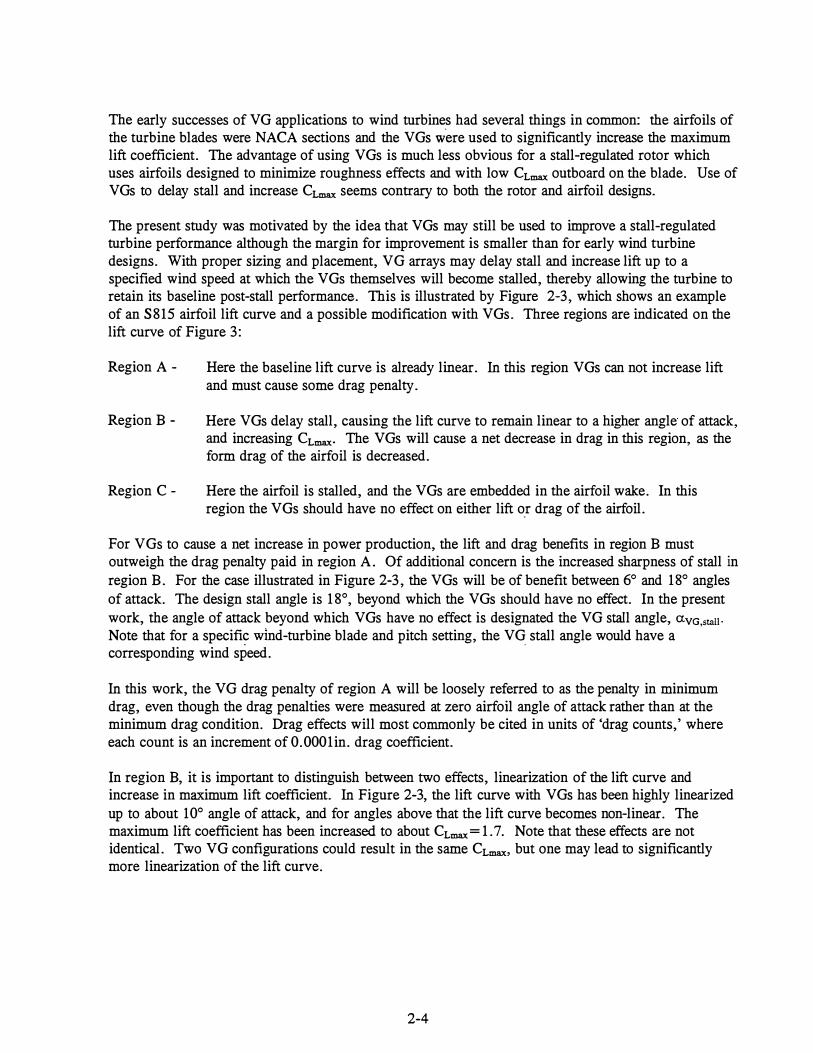
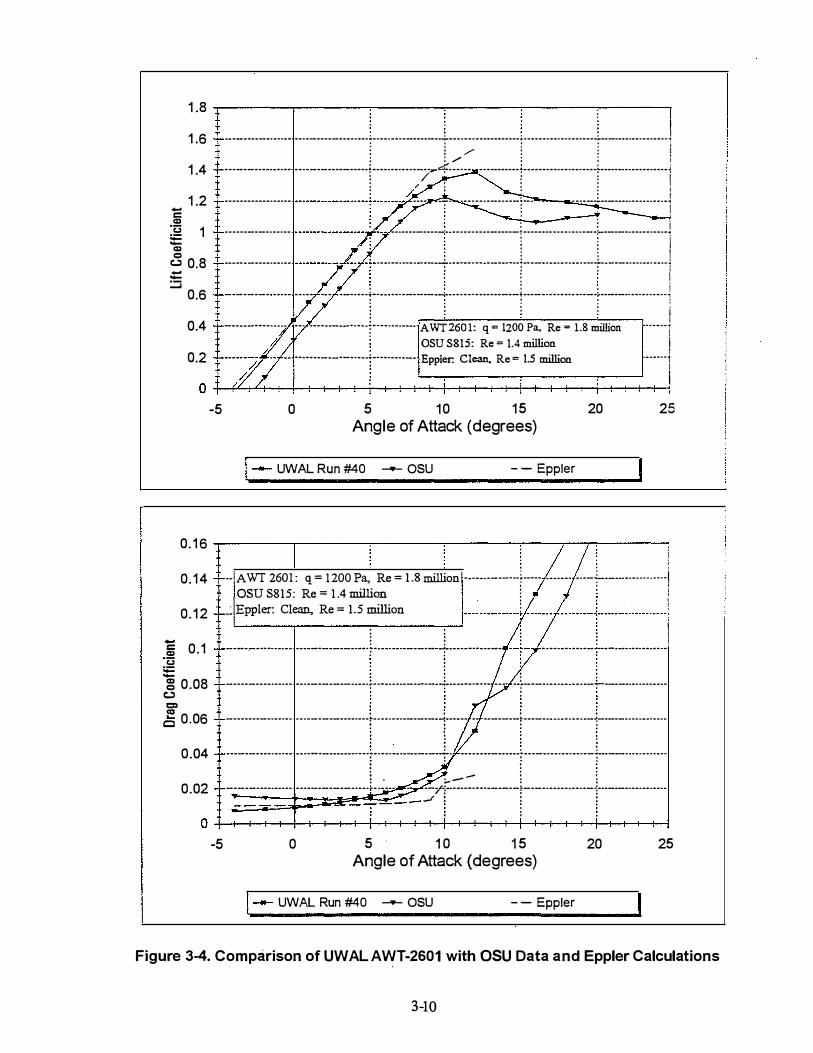
Figure 3-4 shows a comparison of UW AL measurements of the A WT -2601 to previously-reported S815 data from Ohio State University [11], and airfoil performance as calculated by the Eppler Code [12]. While both the UW AL and OSU test data show very good repeatability with themselves, the results from the two tunnels are significantly different. Before comparing these curves, it should be noted that the tests had several differences in both experimental conditions and methodology.

First, the OSU test model was a pure S815, with a sharp trailing edge, while the A WT-2601 was an S815 with a spline-fit applied to achieve a trailing edge which is 6.6 mm (0.26 in) thick. Additionally, the UW AL baseline data were measured at a Regnolds number of 1.8x106, while the highest Reynolds number reported from the OSU test was 1.4xl0 . The UW AL test section was 1.09 x 2.4 m (3.5 x 8 ft) with a 61.0 em (24 in) model, while the OSU test section was 1.0 x 1.4 m (3 x 5 ft) with a 45.7 em (18 in) model. Based on these dimensions, both test sections were nearly 2 model chords wide, the UW AL test section was 4 model chords in height, while the OSU section was 3 model chords high.

The UW AL test used a force balance and used wake surveys only to determine tare drag. Conversely, the OSU test measured airfoil and wake pressures, and then integrated to determine forces. While the UW AL method is more direct, the measurements include forces on end plates, which are only approximately accounted for by the tares. The OSU method is not affected by forces on the model end plates but relies on pressures measured in the tunnel centerline to characterize the entire airfoil.

Both the UW AL and OSU data show the same lift curve slope, but the OSU lift curve is significantly right-shifted, having a higher angle of zero lift, and a lower CL at a=0° than the UWAL curve. The OSU data also show a CLmax which is nearly 0.2 lower than reported by UW AL. The higher Reynolds number of the UW AL test should result is a small increase in CLmai, but not enough to account for the difference seen on Figure 3-4. The UW AL lift curve shows excellent agreement with the Eppler calculation in the pre-stall region.

The UW AL drag curve is not as flat at low angles of attack (in the drag bucket) as either the OSU or Eppler curves. This can be attributed to the method of tare drag which the UW AL test used. That is, wake-momentum measur�ments were used to determine turntable and interference drag at zero airfoil angle of attack, and then this tare was applied over all angles of attack. Note that at zero angle of attack (where the tare was measured) the agreement between the UW AL and Eppler drag values is very good. The OSU test used the wake-momentum method for all pre-stall drag measurements, and while it correctly reflects the flat nature of the drag bucket, the minimum drag values are somewhat higher (40-50 drag counts) compared to the UWAL and Eppler data.

The comparison with data from OSU and Eppler was part of an initial check-out of data quality from the UW AL test set-up and procedures. While it was hoped that the UW AL and OSU data would agree more closely, it was concluded that the UW AL set -up and procedures were sufficient to meet the objectives of the test.

Figure 3-5 shows the baseline lift and drag curves for each of the three models tested. For completeness, Figure 3-6 also shows the moment coefficient curve for the baseline airfoils. Although moment coefficient data were measured for all test runs, moment data with VGs are not presented in this report as the effect of VGs on airfoil lift and drag is of primary importance in the present work.

3-9

1.8 .......-----,.------,.------:------:------:------,

-c a:l

1.6

1.4

1.2

"(3 1 ;;::: -a:l

8 0.8 --:::::::i 0.6

0.4

. . . . I ....... _ ......................... -·----·--------·-·:-- · - · · · · · - ·---·-----;-· · - - - - - · ·-·--·-----!-----·---------·----:----·-···--·------; ; ; ./ ; : I : : / : ; l

- · - - - - - - - -............. - · - - - - ----·--··--t·-·-----·-----;;..-4- - - · - - - - - --·-----t-----------·--------�-------------------1 : " : : : I : /, . : : I

---------------·-- -----------------�- - - - · - - -� ---- ··r · - - - - - - - ------··r· · · · · - ----------··- - · - - · - - · -, . . .

. . : : i ---------------- ----------------7· - - -------------r · · - - - - - - - - ------1·------- - - - - - - - - - - ·r·---------------� ............ .. ------·--·· - · · · - - - - - -LL .................... _ .. __ �_ ................. .................. ! .................. .. .. .. ... .... .. ......... � .. --.. --------- - - - - ..

• • • • ! : : : I

- - - - - - - - - - - - - - - - - - ---·-·t- -- ------+- - - - - ---------i---- - - - - -- - - - -r------ -- - - - - · - ·j - - - - - ··· · · · · · · · · ··· .......... c • . • • . f· · · · · · · · ···· AWT 260 1: q = 1200 Pa. Re = 1.8 million · · · · · ·1

t7 : OSU S815: Re = 1.4 million j 0.2 ·- ·· ····------ - - · · · · ·t- - · · · · · · - · Eppler: Clean. Re = 1.5 million - - - - · ·j

I 0+-��-+��+-��-+��-+-r�+-��-+�

-5 0 5 10 15 Angle of Attack (degrees)

1-- UWAL Run #40 -- OSU - - Eppler

20 25

0.16 ..,.-----...,.-----,.------,.-------:-----;-""j":""-----:

0.14

0.12

i 0.1 "(3 ;;::: -� 0.08

c.,:) = co Q 0.06

0.04

0.02

: ! -- A WT 2601 : q = 1 200 Pa, Re = 1 .8 million ------------+---- · · · · · · · ----�---··· · · · · · · · · · · · · !

OSU 8815: Re = 1 .4 million 1 ·

i • I

-� Eppler: Clean, Re = 1.5 million : !

-------- ---- ------------f--- -- ------ +----------- __[_ _ _ _ _ _ _ _ _ _ _ _ _ L_ ___ __ _ _ _ _ _ _ ! . . . . .

p 0 I 0 ----·--•·••••••• · - - · - - - - - ·-··•-•r•• ............ ., _ ,. .. .,. .. -.. _........................ ........ ••r•• • - • • • • • • • • • • • ·-------··"'•••-•••• . . . . . . .

. . . . -----·-·---·--·- - · - · - - - ·-·-··----:- - -- - · ------·-... : .. ·---- -- -·-·---:-··-·-... ......... .. .. .. .. .. -:---.. ------·------

. . . . . . . . . . . . . . . -·-----------·-- .. .. .... -... _ ................................................... -.. ---- -· - - - ----------.. · · - - - - - - - - - - - - ------------........ .. .. .. .. .. .. .. . . . . . . . . . . . . . . . . .

t ,._.- C I

- · - - --·-------- - - · ·-- - - - · - - · - - -�- -�--- .. --y-�-::: ............... _ .. ___ �- - - - - - - - - - - - - - - -�-·----------···--·

��:+:::::;:;;!��:::i:� .J : : : � - - - _T___ � � 0+-+-�-+��+-�-+-+�+-�-+-r��-+-r��r+-r�

-5 0 5 10 15 Angle of Attack {degrees)

1-- UWP.J.... Run #40 -- OSU - - Eppler

20 25

Figure 3-4. Comparison of UWAL AWT -2601 with OSU Data and Eppler Calculations

3-10

1 .8 .-------�------�------�------�------�----�

-c Cl)

1 .6

1 .4

1 .2

·� 1 ;;::::: -Cl)

8 0.8 --:.:::i

0.6

0.4

0.2

. . ........................................ - - - - - - - - - - -·- ----.; .................... _ .. ____ ....;.. __ ., ................. _ .. ____ ; _______ ..................... __ �----- - · - - - - - - - - · -. . . . . . . . . • 0 ' '

t -·---------··--- ........ ............. ___ ........... �- - - - - - - ---·--··--+--·---

' . .. ................. -;--·------·-·--·---�-------------------

------------------ - - · - - --- - - - ----+·-------------- Baseline Airfoils:

----------------- ---7-----------(--------------- �� = �= : �:� :::::�� ---------------+------·--------- 2603 - Re = 2.5 million

: I . ----:-------.0 --· -- ·----1

0 +-��+-�-+'-+��-+-r�+-��-+�� -5 0 5 1 0 1 5


-- AWT-2601 (35%R) _._ AWT-2602 (55%R) -- AWT-2603 (75%R)

25

0 . 16 ....-------,------:-= ---...,..: -----:-: ---v--1,--...,..: ------,,

� 1 1 ... � i 0 . 14

0 . 12

§i 0 . 1 ·� ;;::::: -� 0.08

c:,:) 1:1:1 Cl:l c 0.06

0.04

0.02

-------- ----- -- - - - - - - - - - - - - -,- - - - -- - -----t------·--- ---�--:! __ __ ,------ -- -- -- -1 �:�:�:�:_::-:: ::-:�:�:�=::1:::::-:�=:J:=::::��:--�;�-L:: :: :�c�: :- :: :: :

. . 0 0 . . . .

........................ ................ --------·---------·---·----------..... _ ........... -....... - - -.. -........................ ........... _ .. _______ ................. .. • 0 • . . . . . . . . . . . . . . . . . . . . . .

--------------- - - - - - - - - - - - ----r----·----------1'--·- - - - - - -�:�:-��;=·----------·----

. . . . ..... .. - ............ ................ -·------·-·--···-·----·--·---------· .. ................ _ ... __ . . - .

2601 - Re = 1 .8 million ----.....---------------- 2602 - Re = 2.5 million

2603 - Re = 2.5 million

0 +-��+-��+-��+-� -5 0 5 10 15


-- AWT-2601 (35%R) _._ AWT-2602 (55%R) -- AWT-2603 (75%R)

Figure 3-5. Baseline Lift and Drag Curves for AWT M odels

3-11

25

0 .-----�----�----�----�----�----�----�----�

-0.05

c -0.1 Cl ·c:; ;.;::::: -Cl 8 -0. 1 5 c Cl E 0

:2: -0.2

-0.25

............... : ....................... .. .. .. .. · ........... _ ............. i---·------·--r-·------.. - - - -:- - - - - - - - -------}- - - · · - - · · · -.. -

. . . .

. . . . . . .

. . . .............. -........................... .......................... _ ......... -............ ..

.. .. ............................................ _ .. _ .. .................... ..

r ..................... ...-- i l l . . . . . . -------- ·--· ··· - --�---· 1::: �:ilHon ............. ............. 7 ....... 12602 - Re - 2.5 million

: 2603 - Re = 2.5 million -0.3 +-t-;-1-"1--+-t-t-1-"1--T-1r-t--t-t----l-,�-t-t-+-!-!-"'!""'"'t-+-t-t--t-t-+-t-t-........r-+-t-t--t-t-i

-5 0 5 1 0 1 5 20 25 30 35 Angle of Attack (degrees)

- AWT-2601 (35%R) -- AWT-2602 (55%R) -- AWT-2603 (75%R)

Figure 3-6. Baseline Moment Curves for AWT M odels

3-12

3. 3. 3 Co-Rotating VG Performance

The effect of VGs was strongly influenced by their chord wise placement, as shown on Figure 3-7. The placement of VGs forward on the airfoil gave the greatest increase in CLmax, and for this VG position, the linear region of the lift curve persisted to a higher angle of attack prior to stalling. Note that the forward placement of VGs on the airfoil, particularly at x/c' = 0.1, actually caused a lift penalty in the linear portion of the lift curve. This penalty was attributed to the VGs triggering early transition from laminar to turbulent flow, thus compromising the designed laminar flow of the airfoils . . The lift penalty for forward-placed VGs was observed for all airfoils tested, most noticeably when the VGs were at or forward of xlc=0.3.

The drag caused by the VGs is consistent with the lift curve trends, with the highest drag penalty (about 45 counts) for the furthest forward placement. Note that although the VGs cause a drag penalty at low angles of attack, they give a drag benefit for angles of attack greater than 10°. This is due to the VGs delaying the airfoil stall, and thus reducing the form drag. Configurations which are most persistent in delaying stall also show the largest reduction of form drag, but will likely have the largest penalty in minimum drag.

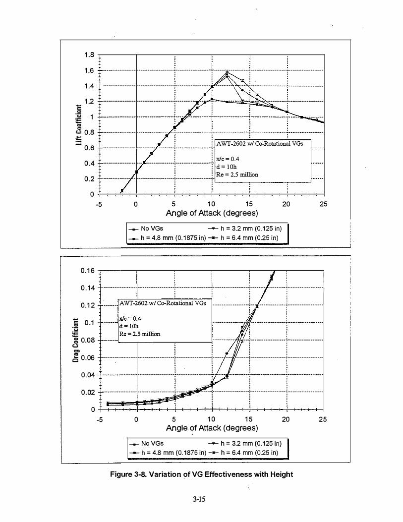
As seen on Figure 3-8, the VGs showed a subtle, but consistent, performance variation with height; larger VGs were more persistent, gave higher CLmax, and caused higher drag penalties. For. the case shown on Figure 3-8, the drag penalties (at zero airfoil AOA), were 19, 23, and 29 drag counts, respectively, for the h=3.2, 4.8, and 6.4 mm VGs. Therefore the 6.4 mm VGs caused a 50 % greater drag penalty, but yielded a CLmax which was only 4% greater than the 3.2 mm VGs.

Both VG performance and drag penalties were directly dependent on array density, as seen on Figure 3-9. The lift curves of Figure 3-9 show the large impact of going from spacing of d=lOh to d=20h; although CLmax is largely unchanged, the difference in the degree to which the VGs have linearized the pre-stall lift curve is dramatic. Also note that the angle at which the VGs became stalled such that the airfoil regained its baseline performance, appears insensitive to the VG array density. These density trends were observed consistently throughout the test for all three airfoils and all three VG sizes.

Another trend which was observed consistently through the test was the dependence of drag penalty on VG array density. This is. amplified on Figure 3-10, which shows that a doubling of the array density leads to an approximate doubling of the VG drag penalty.

3. 3.4 Counter-Rotating VG Performance

As discussed in Section 2.1, counter-rotating VG arrays have an additional variable relative to corotating arrays; they have spacing parameters d = distance between two VGs which form a pair, and D = distance between each pair of VGs. The non-dimensional grouping of D/d is frequently used to characterize VG array geometries, but it requires an additional dimension to completely specify the lateral spacing. For example, there are two fundamental ways to vary D/d. One is to fix D, and change the pair spacing, while leaving the overall number of VGs per unit airfoil span (array density) the same. The other is to fix d, and vary D, which would change the array density.

3-13

1 .6

1 .4 ---------.................. ...... ..... ......... _ ......... ............... ':' ........................ -...... ...

1 .2 ............................................ --------........................................ ...

-c Ql '(3 1 :;:: -Ql C)

t.:) 0.8 --:.::i

0.6 -----------·····- - - · - - ----------L. ................ J.. A Wf-2601 w/ Co-Rotational VGs . .

0.4 - ---------····· -·------------·--·�- - - - ---·-----------.!-- h = 4.8 mm (0. 1 875 in) � � d = lOh = 48 mm

0 2 ..... - - · - - - - - - - -- - · - - -i ........... _______ j __ Re = 1.8 million .

0 +-��-+��+-��-+��-+-r�+-�-+-r,_+-�-+� -5 0 5 1 0 1 5


1--- No VGs -- xlc = 0.1 -- xlc = 0.3 -- xlc = 0.4 ___. xlc = 0.5 ,

25

0. 1 6 ...,..----...,-----...,.._---...-----.----za---.,,-----

0.14

0 . 12

; I ---- ------- ·----- ---------------- · - -r··--- · ------ -------1- · ----------------··r··- -- - - - - - - · - ··r· ·----- ----· - - · · · ·1 ----- A WI -2601 w/ Co-Rotational VGs �- - - - · · · · · · · ------· . ····--·------�----··· · · · · · · · · · · ·

i 0 . 1 ·c::;

___ h = 4.8 mm (0. 1 875 in) d = 1 0h = 48 mm

:;:: -� 0.08

t.:l· = cg c 0.06

0.04

0.02

Re = 1.8 million . . ' . - ....................................... -.. -... -----··--·-..... -

----------·-··-- --·----------·-·t··--·--·----------1- - - - - - - · . --. . --:---------;----------�-·---------·------

. .

. . . . . -·· - ----................ - · - - - - - - - · -----·-.......... ..................... ..... ........... -.... ... ------·----·----- - - · · · - - · · -.. -------·---·----· . . . . . . . ' . . . . . . . . . . . . . . . --�------�-------�------�-----�-------1·----------------r- - - ----------·--i----------·-----·

0 +-��-+��+-�-+-+�+-�-+-+�+-�-+-+��-+� -5 0 5 1 0 15


1-- No VGs -- xlc = 0. 1 -- xlc = 0.3 -- x/c = 0.4 ___. x/c = 0.5 ,

25

Figure 3-7. Variation of VG Effectiveness with Chordwise Placement

3-14

1 .8

1 .6

1 .4

1 .2 ... c Q) 'E 1 ;: -Q)

8 0.8 ... -:::l

0.6

0.4

0.2

0 -5

0. 1 6

0 . 14

0.1 2

-0.1 c

Q) 'E ;: -� 0.08

c.:l = ca c 0.06

0.04

0.02

0 -5

- - -------·--·-- --·-------------r---·----------1·-----�---------;-----------------r-----------------

. . . . . . . ---·----·-··-- --··-----·-·-----t-·-··--·-------· ........ ............. .. ...... "'-----------------�-----·--·--··-·-

--------·----· -···-·-·---·----·�----·-··- ..... .. T.. --- - ---·----·�·-------·-·------

. . . . • t t • �:�:�:=:::: ::::�:�:=��-��:: . .. ::�:�:�:r=��l:�::�:=::::r: _____ _____ _

1 1 A WT-2602 w/ Co-Rotational VGs -----·--···--- --·--·-· -------! ......................... _ .. __ --:-

. . . . l l x/c = 0.4 --------·-···· - - · ---------·-··;-····----------1 d

= 1

Oh . i Re = 2.5 million

-----..... -......... ... -----------.. - · - - - -"----- ---·-·-------.......:.. : : '------...-------.-----'

0 5 1 0 1 5 Angle of Attack (degrees)

-- No VGs -- h = 3.2 mm (0. 125 in) -- h = 4.8 mm {0. 1 875 in) -- h = 6.4 mm (0.25 in)

20 25

. . I --------·-···· .. ······-----·-······r-····--·-- ·--····t--·····--···----··:········ · - · - · · · -:- · - · · · · · · · · · · · · · · ·! �---- A WT-2602 w/ Co-Rotational VGs .....••..•. .......• L ..... ......... 1... ................ .

. . --,-·----·-------···---------------·-·· . . . . . . . . . . . . . .

I • I I -·---·-····--· ....... _ .. _,._,._ ..... __ .t---··------------i--·--- .......... ----t---····-----·--··-�------------------. . . . . . . . . . . . . . .

I ' 0 t . . . ,. . . . .. .., ... ____ .................... --·--·-----·----··-·-··· .. ·-------· .. - ........... -·----·--.. ----··--·---···---·-------·-- .. .. .. .. .. .. .. ..

• • I I .. . . . . . . . . . . . . -·------··--·- -···---.. - - - - - - -r----·- ----l--------------r-----------------1---------------·-


-- No VGs -- h = 3.2 mm (0.125 in) -- h = 4.8 mm (0. 1 875 in) -- h = 6.4 mm {0.25 in)

20

Figure 3-8. Variation of VG Effectiveness with Height

3-15

25

1 .8

1 .6

1 .4

1 .2 -c CD

"ti 1 :0::: -CD Q

c:.,:) 0.8 --:.::i

0.6

0.4

0 .2

0

0 . 1 6

0 . 14

0 . 1 2

-0 . 1 c

CD "ti :0::: -� 0.08

c:.,:) CJ:I <a Q 0.06

0 .04

0.02

0

-5

-5

= . . . I ·················· ·····---------·-··r· · · · · ···-········r····--· -······-···r······-········-··:······· · · · · · - · · · · · ·1 .................. · · · · ··············-·[·········--- . ·. - - . ------t�·-················t··-·-·············1 ······-·········· · · · · · · · - · - · -··---�- - - · · . . ....... ..:....................... . ..... .:.. ................... J

..;. : : : i - · - · ············ · · · · · · · - · - · - - · - - ········-·-·-·-i· · · · · · · · · ···········t····················:···-····· · · · · · · · · · ·j

l . � ! ·•···•····• · · · · · · · · · · · · · · - · · -·---�·-·······-·-·- ··+·iA WT-2601 w/ Co-Rotational VGs

r'·--··

l : : i • • I ······-·········· .... · · · - - · - · · - · ·

t· · · · · ·············

l··j��; �-�-� (0. 1 25 in) t· · · · ·

j • ' . . I ................. .. .............

_

. · - · ·t· -----------·····i·· Re = 1.8 milhon ! ..... . : : : :

. . . . . . · · · · - · · · · - · - -·---�---······-·-····...;. ........ ..... . ..... l .. ................. .:... .................. J . • . • I

0

! ! I , . : ! I

5 1 0 1 5 Angle of Attack (degrees)

20 25

j-- No VGs -- d = 1 Oh -- d = 20h -- d = 30h -- d = 40h I

. . 0 0 I 0 :

....................................... - - - · - - - - - - - - · - - -:- · - · · - - - --------�· - · - - - - ----------r··--- ............................ 1 ....... _ ......... .. .. .. . .. .... .. .. . --: AWf-2601 w/ Co-Rotational VGs ; . ; . . h = 3 .2 mm (0. 1 25 in)

r· · · · · · · · - --····--; · · - - · · · · · · · · - - · · ·-r-·········· · · · · · · · -,·

..... xfc = 0.5 �---·········-· --�---·--···········-.J-----· · · · · · · · · · · ·

Re = 1.8 million l l 1 ] --------------- ---------------r----------------1------------ ------r------------------1---------------- , ------------------ ----------------�- - - - - - - - - - - - - · ·r··----- ------··-r··----------------1----------------

--------·-··-·--- ............. _.,. ___ .. _____ ................... _________ --------------·--·------· --··-- .. -·---- - - · - - - - - - -. . . . .. . . . . . . . . . . . . . . . . . . . . . --------------- --------- - - - - -....:.- - -------1·------------------r·----------------�------ - - - - - - - - - - -


20

1-- No VGs -- d = 1 Oh -- d = 20h -- d = 30h -- d = 40h I

25

Figure 3-9. Variation of VG Effectiveness with Array Density

3-16

-c Q)

"C3 ;: -Q) Q

c.;) = ctl .... c

0.02 -r---.---,,---....,----:---.-----:------,.--..,.----,----:

0.01 5

0.01

0.005

AWT-2601 w/ Co-Rotational VGs h = 3.2 mm (0.125 in) x/c = 0.5 Re = 1 .8 million

. . . "' ..................... �------·- '!'-··--·--·---!---------. . .

: : �: �: �: : : - - - --·-·-······--·--··-- - - - - - - -· ----------- · · - · · · ·········:· · · · · · · · · · -T--···-···r- · · · - - · · · · · j : I . !

----------� ................ · · ·1---------�-----------t----------- -------·- -··t·--------t---- - · · · - - -:··-------r ----- --....... - i . : ! ! : : i

0 ++��· ��· �· �� . . H,-rlrr�· ·

-5 -4 -3 -2 -1 0 1 2 3 4 5 Angle of Attack (degrees)

1-- No VGs -- d = 1 0h -- d = 20h -.- d = 30h -- d = 40h I Figure 3-1 0. Impact of Array Density on VG Drag Penalty

3-17

Because of the additional spacing parameter, a comprehensive sweep of parameter space was prohibitive for counter-rotating VGs. Thus, the UW AL test took the following approach:

1. Co-rotating VG arrays were used to sweep out parameter space, as indicated in the test matrix of Figure 3-2. These test runs were used to identify trends due to VG size, chordwise placement, and array density.

2. For several cases of interest, counter-rotating VG arrays were tested and compared with their equivalent co-rotational arrays. For this purpose, an equivalent array had VGs of the same size at the same chordwise location and the same number of VGs per unit airfoil span (array density). Based on previously published results on counter-rotating VGs, it was expected that D/d=4 would be close to optimum. Therefore, for most counter-rotating tests, D/d was fixed at 4 and the array density was varied by selecting the desired value of D .

3. For one case of fixed VG size and array density, the effect of pair spacing was investigated by varying D/d.

In general, counter-rotating VG arrays were evaluated by testing configurations which had co-rotating equivalents and comparing the performance. Figure 3-1 1 shows such a 'check-point' comparison, where VG arrays of two different densities are shown. Array #1 had density of 21 VGs per meter of span, and Figure 3-11 shows that for this case the counter-rotating array gives a CLmax which is 0. 15 higher than the co-rotating equivalent. However, for an array with 10.5 VGs per meter span (Array #2 on Figure 3-11) the counter-rotating VGs led to a much less linear lift curve and a CLmax that is 0.2 lower than the co-rotating equivalent.

This sort of on-design/off-design behavior was observed for all the counter-rotating VG configurations tested. That is, for some cases the counter-rotating arrays would perform significantly better than their co-rotating equivalents, and for other cases significantly worse. This may be attributed to the nature of the flow fields for these arrays. With the additional D/d spacing parameter, optimal counter-rotating V G arrays are dependent on all the physical dimensions of the airfoil and array.

Figure 3-12 shows a pair spacing study for counter rotating VG arrays, with fixed array density (21 VGs/m), and variable D/d. As Figure 3-12 indicates, a very subtle dependence on D/d was found for this case; D/d=4 performed only slightly better than the other spacings investigated and D/d=2 was the worst. Given the above discussion, this is not expected to be a general result. For another array density, optimum performance may be more strongly affected by D/d spacing. However, these spacing studies were somewhat time consuming and the test resources did not allow for detailed testing of these trends.

3-18

2 �-------.----------------�----------------------�

1 .8

1 .6

1 .4 ...................... -................. ------------.................................... __ .. ..

-.§ 1 .2 --------------- ·--------------·:-·--·- - -----;----------------;-·=· --��;.::-_: � : : : : ___ .....,. 'ai 1 --------------- ---------------- : ---------------+----------------�----------------+----------------.J 8 . : : : § 0.8 r-·--------·-····· --------- ···-+-----------·----+--------

A WI�2601 :

0 6 ---------······· ----- -----------l-----------------..:. ________ _ · ' � l h = 4.8 mm (0.1875 in)

0.4 ----------····· ---------------i---·····---------�----·-···· x/c = 0.3

0.2 1 1 Re = 1.8 million . . . .

------ -----------------r·--------------r-·---------------- 1----- - - - - - - - - - - ---·-r· - -----------------

0 +-��-+�+-+-�-+-r�+-�-+-+�+-+-�-+�4-+-�-+.�. -5 0 5 1 0 1 5

Angle of Attack (degrees) 20 25

-- No VGs -- Co #1 , d=1 Oh -� Counter #1 -- Co #2, d=20h -- Counter #2

0 . 16 -,-------r-------c------o------..,-�--c------:1 : . : r : , 0 . 14

0 . 12

i 0. 1 ·c::s :;:: -� 0.08 (..) = ca c 0.06

0.04

0.02

-----------��:��---------r· ·------------·r··--------------J7-1 ----------T----------------1 -----�-----------------7' - j·--------------:------------------1

: I . .., .

h = 4.8 mm (0.1875 in) : : 1 ------- x/c = 0.3 ----�-------------- --. f-----------------1-----------------

Re = 1.8 million 1 ' I · -----·-------- ............. --------·-�-----·------·--�----------·- .. - r------··---------:----·------·--··--

1 � r � : -------------- ----------------�---------------�-------- - -- --f------------------!------·----------

: : · v : :

: : ./- : : ; : ,.-: ; . : --------------- ----------------r--------------� - ----------r------------------r------------------------------ ----------- ------1·----------------r----------------r··---------------

o+-�-r��-T��-r��-T��r4-r�� -5 0 5 1 0 15


-- No VGs -- Co #1 , d=1 Oh -� Counter #1 -- Co #2, d=20h -- Counter #2

Figure 3-1 1 . Comparison of Co-Rotating and Counter-Rotating VG Arrays

3-19

-

2 �------�------�--------�------�------�-------.

1.8

1.6

1.4

: . I ----·------------- .... .. ............... _ _ _ _ _ _ _ ... __ '"':" __ ,. _ _ _ _ _ _ _ _ _ _ _ ..... .......... �- - - - - - - · ------ ----; - - - - - - - - - - - - - - - · --- -:-·-----------------· ..

. . . . . . . ··-·----------··· · · - - - - - - - - - - - - - - -T ....... ... .... .............. _ .......... :- · - _ _ _ _ _ _ _ ............. ;---- .. .. .. ... ..... ___ ·;-------··-----------

-� 1.2 c.:l -= a; 1 . .

-----------·--·-- ----------------· .. .. ................... ....... ................ :- - -.......... ............................. : ...... .... ...... ...... .............. ...... : ... ........................ .............. .. ..

0 u

. . . . . . . . :: 0.8 • • 0 •

-- ... ..... .. _ _ _ _ ....... ...... ..... ... ............ ............... .. ......... 7 .. .. .. ..................... _ ....... - -:--- ................................ ------ � ..... .............. ..... -... ..... ................ �--------·---- ............. --

--1 . ; : AWT-260 1 0"6 r··----------·--·--· -·--- -------·--··r· · - ·------------·r· · - - -·-----

h =

4.8 mm

(0. 1 875 in) 0. 4 -----------·--·-- ·------------ - · - - · ·t· · · - - · - ----------··t· · - - - - - - - - - - - x/c = 0.3

� 1 d = l Oh 0.2 - - - - - - - - -----· ----------------·-T· · · - - ··-----------·;- - - - - - - - -----

; : ��------�--� 0 +-�+-��-+-+-+��·-;-+-+��·�.�.-+.-+��+-+-�-+-+�

-5

0.1 4

0.1 2

g 0.1 ] � 0.08 t.:) = . J5 0.06

0.04

0.02

0 5 10 15 Angle of Attack (degrees)

20

/ -- No VGs -- D id = 2 -- D id = 3 -- D id = 4 -- D id = 5 J

··-------.............. ............ ... --·------- - - - - - · · - - f - - - - - - - - - - - - · · - · - - - -:- - - -------------------- ...:-------

0 • • . .

; ; -·--... ---- - - - - - · - - - - ---·------ - - - - - · - - - - -r-·----------- - - - - - - - ·r·----------·--·------·-\- -- -----·-------·

AWT-2601

h = 4.8 mm (0.1875 in) x/c = 0.3

----- d = lOh '-----,..-------'

. . . ............... - - - - - - - - - - --·----·---------- ........... -----·------.... ·--. . . . . . .

. . . �-.. ·-·--- - -- - - - - - - - - -:-·--· .. ---·--

.

. . . . .

- - - - - - - - - · - - · - - · - - -------------------·j· · - - - - - - - - - - - - · - - - -;-------- ---

. . . . - - - · -·------- - · · · · · _ _ _ _ _ _ _. ............ ; .............. � ............. - - - - - - - - - - · · · -;.. .. ----- - - - - - - · · · -.; .... ................... _ ................. .. . . . . . . . . . . . . . . --��

�;;

;=:=

��

��

��

.

. -;·-------------- -------------- -- - - - - - - - - - ·1·-----------------··r·-----------------

0+-+-+-r-��-+-+-+-r-r��,_+-+-+-+-r-�-+-+� -5 0 5 10


1-- No VGs -- Old = 2 -- Did = 3 -- Did = 4 -- Old = 5 I Figure 3-1 2. Pair Spacing Study for Counter-Rotating VGs

3-20

20

25

3.3. 5 Effect of Leading-Edge Roughness

One potential benefit of VGs is recovering airfoil/blade performance lost to soiling. Although the new NREL airfoils are less sensitive to soiling than previous airfoil families, they still experience soiling losses resulting from increased drag and decreased lift. To investigate this effect, the standard NREL roughness template [11] was used to simulate leading-edge grit roughness (LEGR). A #40 lapidary grit was used, resulting in a roughness of k/c=0.0014.

Figure 3-13 shows the impact of LEGR roughness on the A WT-2603. Note that this airfoil represents the 75% span location for the A WT -26 blade, a location for which bug soiling is to be expected. As seen on Figure 3-13, LEGR impacts the airfoil performance in several ways. Lift values are decreased in the linear portion of the lift curve, the lift curve becomes non-linear at a lower angle of attack, and there is a 0.2 drop in CLmax· The LEGR also caused a 45 count drag increase over the clean airfoil.

The drag penalty and the shift in the linear portion of the lift curve are both due to the LEGR spoiling the laminar airfoil flow, and VGs were unable to recover performance lost to this effect. The VGs did delay the onset of stall on the soiled airfoil, and by a.=6° the airfoil with VGs had recovered lift values equal to the clean airfoil. From Figure 3-13 it is apparent that the VGs decreased the airfoil sensitivity to roughness for most angles of attack, and slightly increased it for angles between 12° and 16°. With LEGR applied, the VGs resulted in an additional 17 counts of drag penalty for low airfoil angles of attack.

3. 3. 6 Reynolds Number Effects

Due to the geometry of the AWT-26 blade, Reynolds number (Re) varies along the blade radius. Figure 3-14 shows the effect of Reynolds number on clean airfoil performance for the A WT -2602 model. The general trends are that CLmax increases and CDmin decreases with increasing Re, and the magnitudes of the lift and drag increments diminish at high values of Re. The impact of Re on VG effectiveness is shown on Figure 3-15, and the airfoil with VGs follows the same trends as described above. Several studies were performed at the beginning of the UW AL test to verify that the Re effects were consistent and predictable, and the results shown in Figure 3-15 are typical of those seen for all cases.

3.3. 7 VG Yaw Sensitivity

For an airfoil, a yawing motion relative to the free-stream can lead to a change in the VG angle of attack, which can in tum lead to a change in the strength and effectiveness of the vortices generated. Note that the equivalent condition for a wind turbine could be caused by changes in the radial out-flow component along the blade, and that the yaw degree of freedom for an airfoil should not be confused with the yawing motion of a wind turbine.

Due to the mounting methods of the UW AL test, yawing of the airfoil was not possible. Therefore, the impact of yaw on VG effectiveness was simulated by changing the VG angle of attack, a.vG· The idea was to determine at what a.vG (or equivalently at what yaw angle) the VGs would lose their effectiveness. The baseline a.vG was 20°, with angles of 17.5°, 15°, 12.5°, and 10° also tested. Figure 3-16 shows the variation of VG effectiveness with a.vG, and it is seen that the VG performance begins to fall off slightly at a.vG= 12.5°, and drops more noticeably at a.vG= 10°. Although the lift

3-21

performance at 15° and 20° is nearly equal, the 15° drag penalty was twice that for the 20° array (22 and 1 1 counts, respectively). For angles less than 15°, small changes in drag penalty were observed.

3-22

1 .6 I : : : : I

l : : : : I

: ·: �:�:�:�: ·

. :: .: -�:�:�:�: ::�::· :: :�:�:-�·::: :: .: :�r� �: :·:·::·· ::J . : ?.- " : i y' : : : . . " . . I c 1 ------------····-- ········--------·--·--·--·-·· ....... .;. ..... ..,...._� .. ;............ - ---�---·-············� -� . ---t- �, : · I ·- . _,.,. . . - . - . . . --- � � � 0. 8 ·---·--··········· ····--····--·--·--+�·.2.': ·-·--··--·i···-·--·--·----····· j··············� - 4 ' ' ; I

:S 0.6 .................. ········-----�"-'(+ ·--·- A WT-2603 w/ Co-Rotational VGs j +·················-� 0.4 t · · - - ·· ·r � - - ·· · ·· :: io� mm (0. 1875 in) k ·- · · · ·:

-c C)

'C3 ; -

: x/c = 0.4 : I 0.2 ····--------··; ¥----------·-·-·-··t··

··· Re = 2.5 million --:···················-� 0 ' I

-5 0 5 1 0 1 5 Angle of Attack (degrees)

20 25

-- 2603, Clean -- 2603. LEGR -- Clean with VGs -- LEGR with VGs

0. 1 6

0. 14

0. 1 2

0 . 1 h = 4.8 mm (0. 1 875 in)

·-------- d = 1 Oh x/c = 0.4

� 0.08 -------- Re =.2.5 million c..J

= co::l 0 0.06

0.04

0.02

0 -5 0 5 1 0

Angle of Attack (degrees) 1 5 20

-- 2603, Clean -- 2603, LEGR _,._ Clean with VGs _,.._ LEGR with VGs

Figure 3-1 3. Effect of Leading-Edge Roughness

3-23

-c

1 .4 .,..----r---------:------:-----.,...------;------, 1 .2

1 -·--------·-···- ...... ........... _ ... _ _ _ _ _ , .... � .. ----

I I . - --------�-----------·------�-------------------i : : i : I ----------+----------------+--------------------�---- _ _ _ _ _ _ _ _ _ .J . . . . . . . . . . . . .

:§ 0. 8 ·i·-----------------:····--------------:-··--·--·---------;------------------1 .... . . . . 1 � l l l 1 � . . . . § o.s r······-· ·· ·· ·· ·-··· ··-··r· ·· ·-·-·-·r ·······-·-·-r····· ····· ··r··· ·· ·· ·· ·l

0. 4 -------········· ... ----------····! ........... ·······-+----------......... ; .. ---------..... -+····· .. --········ '"1 : : : : I

0.2 ............. . mm•n·•·····r·· ·· ·-·-·-+mm•n•••·-W WT ·2602, 'No va, f ·j : I 0 +-+-�-+��+-�-+-r�+-�-+-+��-+-r�+-�-+�

-5 0 5 1 0 1 5 20 25 Angle of Attack (degrees)

--- 1 . 1 4 million -- 1.8 million --- 2.5 million -- 3.0 million -- 3.4 million

0 .1

f I

0. 08 1·-----·········· ······ ---·-·····-··· · --·-·-·r ·· ··· -····r ·· ·····--- �---- ---·- -- - j

..... . . . . . ! 0 06 -------·········· ···--·-····-----·�---··-----------�----- ·····-----�--------·-···-----+----·-············ t.:l • • • • •

= : � � :

� � 0. 04 --------·--··-·· ----------------�------··--------� --------------:------·-----------;----·-····-------

Cl

0.02

: : : ..... r-··--···- --+JAWT-2601 io v"' !... ..

. . . . . . . . . . 0 +-+-�-+��+-��-r��+-r-�-+��+-+-�-+��


20 25

-- 1 . 1 4 million -- 1 .8 mil l ion -- 2.5 mil l ion -- 3.0 mill ion ......- 3.4 million

Figure 3-14. Reynolds Number Effect on Clean Airfoil

3-24

1 .6 ...-----...,...----.......------,------.------:------,

1: 1 CD .t) � 0.8 c.;)

:;:= 0 6 --------·---·-··-· · · · · · · - - - - - - - -_ __ .L_ ___ A WT-2603 w/ co-rotational VGs ..-1 • 1 :

0 4 ---------·-··--·-· ....... __________ .L_ _ __ h = 4.8 mm (0.1875 in)

· : x/c = 0.4

0.2 Low Re = 1.8 million High Re = 2.5 million

0 +-r-��+-r-�-+-r��:-+.-r��+-��-+��r-�

-c

0.08

·� 0.06 :;:: -Q) Cl

c.;)

� 0.04 c

0.02


20 25

--- No VGs, Low Re -- No VGs, High Re -- VG d=1 Oh, Low Re -- VG d=1 Oh, High Re -- VG d=30h, Low Re -- VG d=30h, High Re

AWT-2603 w/ co-rotational VGs h = 4.8 mm (0.1875 in) x/c = 0.4

------- Low Re = 1.8 million High Re = 2.5 million

0 +-��-r-r-+-+-+-+-+�_,��r-r-r-� -5 0 5 1 0


- N o VGs, Low Re -- No VGs, High Re -- VG d=1 Oh, Low Re _..,_ VG d=1 Oh, High R e -- VG d=30h, Low Re -- VG d=30h, High Re

Figure 3-1 5. Reynolds Number Effect on VG Performance

3-25

20

I I I I j

-

1 .6 ..,..----.,------:-----.,.-----,-----.,.-------,

1 .4 -------------- -- ----------------------------------------· � :·--------- -- -T·--- -- -- - -1 1 .2 -=�-=·--"=.!- .,_;:-·-------------�-----------------

. . . . ·-·--···--------- .... ........... _.., ________ . _______ .. .. .......... � - - - - - - · · -.. · - · -----·----· - - - · - -. . . . . . . . . . . . . . . . . . . . ---------·---·-- ... ... .......... _.,. ________ . - - - · ----------...... - - - - · - - - - ·-··--·--......... ...... .. ....... ....... .... ..

:s 0.6 ------�------·-··· --·------ - - - - - - - - ·+- - - - · - -·-----· ---+- · - - - - - · · - -------·· t ----- - - - - - - - - - · -·--·�-·----------------. ' . .

0.4

0.2


20

-- No VGs -- 20.0 deg -- 15.0 deg -- 12.5 deg -- 10.0 deg

25

0.08 �----.--------------.CTT"""----------,.

0.07

0.06

-� 0.05 "t:i :;: -g 0.04

(,.') = ca c 0.03

0.02

0.01

I : : . I ---------------·-- ------------------r----------------l------------ -T-------------------r----·------------1 0 I I o

............. .................... -- ............ ... -- - - ............ ........ ......... .............................. "'1.................. .. ---.... --- ........... - .... - - - - . - --··---------- . .... - .... . . . . . . . . . . . . . . . . . . .

- - - - -----·------ - - - - - - · - - - - - - - - - ·!'-····-----------�-·-·- - -- ---··r----- ---··- - - - - -·--t----- - - - - - - - - - · -

- · - -----··-··· ·-··----- ·-- - --··-----··- · - --·-·---- .......... . . . . . . . . . .

. . -·-·-----··- · - - · - · - · - · - - - ---------------·-. .

A Wf-2603 w/ co-rotational VGs ----·---------- --------- -------�----- -------l··------

h = 4.8 mm (0. 1875 in) . � x/c = 0.4 ·��;;;1!��-!! ...... t··---·----·------�----·-- · ,_R_e_=_2,.5_rn_il1_io_n __ :------'

0 +-+-+-�-+-+�-r�;i�-+-r-r�·-+-+-r-r,_+-+-r-��-+�� -5 0 5 1 0 1 5


-- No VGs -- 20.0 deg -- 15.0 deg -- 12.5 deg -- 10.0 deg

Figure 3-16. Effect of Yaw on VG Performance

.3-26

25

3.3.8 Summary of Results

The UW AL wind tunnel test was a comprehensive sweep of VG parameter space for three airfoil sections which are characteristic of the A WT-26 rotor blade. A summary of all co-rotational cases is shown in Tables 3-2, 3-3, and 3-4. The following general trends were observed throughout the UWAL test:

1) VGs placed at or forward of x/c=0.3 seemed to disrupt the laminar flow of the airfoil, with a corresponding increase in drag penalty and a decrease of lift in the linear portion of the lift curve. The farther forward the VGs were placed, the more noticeable the effect.

2) The magnitude of CLmax' and the extent to which VGs delayed airfoil stall was - strongly dependent on the chordwise placement of VGs - weakly dependent on VG height - nearly independent of VG array density.

3) Forward placement of VGs increased both CLmax and the angle at which the VGs became stalled.

4) VG array density affected the nature of the pre-stall lift curve. The higher density arrays had more linear lift curves.

5) Increased VG performance (e.g. higher CLmax, increased linearity of lift curves, greater amount of stall delay) was always associated with a larger penalty in Comin·

6) For some cases counter-rotating arrays showed better performance than their equivalent co-rotating arrays, and for some cases, worse. Optimal counter-rotating performance seemed to be very dependent on the specific geometry.

3-27

Table 3-2. AWT-2601 , Summary of Co-Rotating VG Configurations Tested

Run q height array chord effect on ..1 CLmax ocvGstall ..1 CDmin # (Pa) (mm) density

(dlh)-location - linear CL e) (# counts)

40 1200 None No VGs N/A CLmn=1.41 Cnm;n= 90

46 1200 3.2 10 0.1 Bad (R: .05) . 32 27 40 47 " " 20 " " .25 " 26 48 " " 30 " " . 27 " 18 49 " " 40 " " . 07 " 12 51 " " 10 0.3 Mod. (R: 0.2) .27 19 31 52 " " 20 " " .19 " 18 53 " " 30 " " .26 18 13 54 " " 40 " " . 13 " 9 195 " " 10 0.4 Slight . 31 16 14 196 " " 20 " " .22 " 6 55 " " 10 0.5 None .16 13.5 13 57 " " 20 " " . 13 " 7 58 " " 30 " " .08 " 4 59 " " 40 " " . 05 " 2

32 1200 4.8 10 0.1 . Bad (R: .05) .36 30 45 34 " " 20 " " .29 " 28 35 " " 40 " " .07 " 14 36 " " 10 0.3 Mod. (R: .02) .34 20.5 35 37 " " 20 " " . 31 " 21 38 " " 30 " " . 15 " 14 39 " " 40 " " .08 " 10

197 " " 10 0.4 Slight .32 18 17 198 " " 20 " " .27 " 8 41 " " 10 0.5 None .23 15 21 42 " " 20 " " .18 " 12 43 " " 30 " " . 07 " 7 45 " " 40 " " . .04 " 6

60 1200 6.4 10 0.3 Mod. (R: .02) .24 22.5 38 61 . " " 20 " " . 19 " 22 62 " " 30 " " .08 " 12 63 " " 40 " " .07 " 9 199 " " 10 0.4 Slight .25 19 26 65 " " 10 0.5 None . 18 16 24 66 " " 20 " " . 11 " 13 67 " " 30 " " .05 " 8 68 " " 40 " " .05 " 6

3-28

Table 3-3. AWT-2602, Summary of Co-Rotating VG Configurations Tested

Run q height array chord effect on ti Ctmax OCyGstall ti CDmin # (Pa) (mm.) density location linear CL CO) (# counts)

(d/h) 156 2400 None No VGs CLmax=1.23 Cnm;n= 56

159 2400 3.2 10 0.4 None .31 16 18 160 " " 20 " " .31 " 9 162 " " 10 0.5 " .22 14 11 163 " " 20 " " .16 " 5

" "

175 2400 4.8 10 0.3 Mod. (� 0.2) .35 19.5 31 176 " " 20 " " .34 " 16 164 " " 10 0.4 Slight .33 17.5 21 165 " " 20 " " .33 " 10 166 " " 10 0.5 None .23 15.5 14 167 " " 20 " " . 19 " 6 168 " " 10 0.6 " .08 14 9

169 2400 6.4 10 0.4 Slight .42 18.5 28 170 " " 20 " " .26 " 13 171 " " 10 0.5 None .23 16.5 21 172 " " 20 " " .18 " 9 173 " " 10 0.6 " .11 14.5 14

3-29

Table 3-4. AWT-2603, Summary ofCo-Rotating VG Configurations Tested

Run q height array chord effect on b. CLmax ocvGstall b. CDmin # (Pa) (mm) density location linear CL (0) (# counts)

(d!h) 97 2400 N/A No VGs Cr.m�Y= 1 .20 Cnmin= 75

1 13 2400 3 .2 10 0.4 Slight .25 15.5 1 8 1 14 " " 20 " " .22 " 6 1 15 " " 30 " " . 16 " 4 1 18 " " 10 0.5 None . 19 14.5 12 1 19 " " 20 " " . 14 " 5 120 " " 30 " " .08 " 2 122 " " 10 0 .6 " .01 12.5 6

99 2400 4.8 10 0 .4 Slight .30 16.5 22 101 " " 20 " " .25 " 10 1 03 " " 30 " " . 17 " 6 1 05 " " 10 0.5 None .23 15.5 14 1 06 " " 20 " " . 15 " 7 1 07 " " 30 " " .08 " 2 1 09 " " 10 0 .6 " .06 13.5 9 1 10 " " 20 " " -.01 " 3

1 27 2400 6.4 10 0.5 None .24 16.5 1 8 128 " " 20 " " . 15 " 7 1 29 " " 30 " " .08 " 3 130 " " 10 0.6 " .08 " 10 1 3 1 " " 20 " " 0.0 13.5 3

3-30

4 .0 Design and Analysis

The results of the wind tunnel tests, combined with insights gained through the literature search, were used to design a VG configuration for full-scale testing. It is important to note that this design and analysis has been performed for the A WT-26 rotor. Specific results, in terms of VG sizing and placement, may not generalize to other rotor designs. However, the general issues, tradeoffs and methods illustrated in the present work may be applicable to a wider class of wind turbine rotor designs. The goals of this phase of the project were to design a VG configuration which

1) best augments the performance of the A WT -26 at low-to-moderate wind speeds 2) does not impact the peak power or peak loads of the turbine 3) leads to no adverse turbine dynamics.

To meet these design goals, VGs would be used to delay stall and increase lift on local blade sections. It was thought that with correct sizing and placement the VGs would be effective throughout a desired wind-speed range and then stall so that the maximum power of the baseline turbine and its post-stall performance remained unchanged.

Referring to the regions as defined in Figure 2-3, for the VGs to yield a net increase in performance, the lift and drag benefits in region B must outweigh the drag penalty paid in region A. The requirement that the VGs do not increase peak power and loads is equivalent to requiring that all modified blade sections are in region C for wind speeds at or above peak rotor power. Additionally, the dynamics of a stall-regulated rotor could be seriously affected by the increased sharpness of stall between regions B and C. However, the sharpness of stall was not explicitly addressed in the present design and analysis as all calculations and trades were performed for steady-state conditions (assuming smoothly varying wind conditions). The impact of the VGs on unsteady blade/turbine dynamics were ultimately assessed during field testing.

4. 1 Scaling of Wind-Tunnel Test Data

In terms of VG height, care must be taken when scaling wind-tunnel results. The wind tunnel tests were all for airfoils of fixed chord = 61 em (24 in.). As the wind-tunnel tests were run near full-scale Reynolds number, VG sizes would appropriately scale by height/chord (h/c). Due to the tapered planform of the A WT-26 blade, a given wind-tunnel height would scale to different full-scale heights at radial blade stations. Table 4-1 shows h/c equivalency .for fixed wind-tunnel VG heights at varying radial stations on the A WT-26 blade. An alternate approach is to consider a VG array of constant fullscale height. In this case analysis must be performed by interpolating between the wind-tunnel data for the heights which were tested.

Table 4-1 . Full-Scale VG Height for Equivalent Wind-Tunnel Scales Full Scale VG Height mm) at

Wind-Tunnel Scale (mm) 25% R 35% R 45% R 55% R 65 % R

3 . 18 5.87 mm 5.94 mm 5.59 mm 5 . 16 mm 4.67 mm

4.76 8 .81 mm 8.91 mm 8.38 mm 7.72 mm 7.01 mm

6.35 1 1 .75 mm 1 1.87 mm 1 1 . 17 mm 10.29 mm 9.33 mm

4- 1

Once the height scaling was completed, the remainder of the dimensional scaling was fairly straightforward. Lateral spacing in terms of dlh, and chordwise placement in terms of x/c, could both be related directly to wind-tunnel test cases.

4 . 2 Constraints I Design Space

The first approach taken to the VG configuration design was to see how the potential design space was limited by various constraints. PROPPC was used to calculate blade angle of attack versus wind speed for each radial station along the A WT -26 blade. At each blade station, angles of attack were related to airfoil data from the UW AL tests, and limits on VG position and size were determined. These comparisons were made directly at 35 %, 55 %, and 75 % radial blade locations, which correspond to the three A WT wind tunnel models tested. Wind tunnel data were interpolated to determine design limits at intermediate positions, and extrapolated inboard of the 35 % station.

Figure 4-1, a plan view of the A WT -26 blade, shows how some constraints limit the VG design space in terms of chordwise placement and height. In terms of the design goals, the only inviolate constraints shown are the forward stall limits. VGs placed forward of these locations would not allow the local blade sections to stall prior to peak rotor power, and they would therefore increase Pmax. Two such constraint lines are shown, for wind-tunnel VG sizes of 3.18 and 4.76 mm (0.125 and 0.1875 in). Note that the constraints show a weak dependence on VG height, as the shorter VGs may be placed slightly further forward on the blade without causing excess peak power. Also note that Figure 4-1 shows no dependency on VG array density. Wind tunnel data showed that even sparse VG arrays will cause excessive stall delay if placed too far forward on the blade chord.

The aft constraint shown on Figure 4-1 comes from practical considerations. Wind tunnel results showed that VGs placed at or behind these locations may lead to a slight drag penalty but would give no measurable increase in performance. The intersection of the aft constraint with the forward stall limits thus forms a fundamental limit to the span wise extent of the array. It is seen that VGs cannot be placed outboard of the 65 % radial position without violating one of these constraints.

The forward drag limit is not inviolate, but VGs placed at or ahead of these locations compromise the local laminar flow, resulting in excess drag penalties (and possible loss of lift) at low airfoil angles of attack. However, it may be desirable to pay these penalties, if performance gains at moderate angles of attack are sufficient to offset the losses. This issue is addressed in the analysis of the following sections.

4.3 Performance Trades Using PROPPC

In predicting the potential of VGs to improve performance, the largest uncertainty was in using measured two-dimensional airfoil data to predict expected three-dimensional blade properties. The UW AL experiments resulted in a comprehensive data base of 2-D �CL and �C0, for a wide range of VG sizes, chordwise placement, orientation, and array density. Using this database to determine an optimal full-scale design implies knowledge of two things: the 3-D aerodynamic properties of each blade section, and how those aerodynamic properties would be modified by the use of VGs.

4- 2

· Root 1 5 % R 25 % R ·

t 35% R 45 % R 55 % R 65 % R 75 % R

. Chord-Wise Constraints /11{ / 1 1 1 Forward drag limit - VGs here compromise laminar flow.

\ \ \ \ \ \ \ Aft effectiveness limit - VGs here have little or no benefit.

- - ..J - - "Soft" forward and aft limits - VGs may be beneficial here but this has not been validated by wind-tunnel test.

S S S S S � Forward stall limit - for h = 3 . 1 8 mm (wind-tunnel scale)

\ '. \\\ \ \ \ Forward stall limit - for h=4. 76 mm (wind-tunnel scale)

Figure 4-1 . Vortex Generator Design Space for AWT-26 Rotor Blade

85 % R 95 % Tip

This distinction is of particular importance to VG design for a stall-regulated wind turbine. Current research shows that the inboard portions of the blade may be subject to significant stall delay, possibly due to centrifugal pumping effects on the boundary layer. If the boundary layer on these blade sections is already modified by 3-D effects, the additional effect of VGs is uncertain. For blade sections experiencing 3-D stall delay, the .6.CL gained by the use of VGs may be diminished. Similar uncertainty exists for the 3-D effects on drag and VG stall angle.

Further outboard on the blade, it is expected that the centrifugal effects diminish and the 2-D section properties more closely approximate the 3-D blade aerodynamics. However, the goals of the current design require that the VG array is entirely inboard of the 65 % radial station where the 3-D effects will likely be dominant. Performance trade studies that use the 2-D wind tunnel results will therefore be dependent on the assumed (3-D) baseline aerodynamics of the rotor and the assumed incremental performance due to the presence of VGs.

In the present work, performance trades were conducted using PROPPC [1]. AWT engineers have constructed a baseline A WT-26 input deck which approximates the rotor's 3-D blade aerodynamic properties at various radial positions. PROPPC calculations were performed with the baseline input deck, and with modified decks to simulate possible VG configurations. In modifying PROPPC input decks, the incremental changes in airfoil properties (.6.CL and .6.C0) were applied directly as measured in the UWAL tests. Annual energy production (AEP) calculations were performed for both the baseline and modified PROPPC power curves, and the percentage improvement was used to evaluate the effectiveness. These calculations were performed for a wide range of design space: VG heights, chordwise placements and array densities. During these trades, the only constraint was that the baseline peak rotor power not be exceeded.

In all cases, the performance trades favored a forward chordwise placement of the VGs. That is, the calculations showed that for forward-placed VGs, the additional drag penalty at low angles of attack would be more than offset by the additional persistence of the VGs at moderate to high angles of attack. The calculations showed this trend even when VGs were placed so far forward as to disturb the laminar flow of the airfoil section. Considering Figure 4-1, this is not a surprising result. The requirement that peak power not be exceeded (forward stall limit) is the dominant constraint outboard of the 35 % radial position. Inboard of this position, the turbine blade is at moderate to high angles of attack over most operational wind speeds and so drag penalties at low angles of attack becomes insignificant.

Another general trend from the PROPPC trades was that the most dense configurations (d= 10h) consistently showed the best performance_ gains. Again, this was despite the fact that the d= 10 drag penalties were approximately twice those for d=20h. The dependence of VG performance on height was more subtle, with the optimum falling between the 3.18 and 4.76 mm (wind-tunnel scale) sizes, and the larger VGs performing only slightly worse.

4.4 Designing for Smooth Stall Progression

During the PROPPC trades, the only constraint imposed was that the baseline peak rotor power not be exceeded, and calculations predicted that VGs could result in up to a 4.5 % gain in annual energy production for the A WT-26 rotor. Within this constraint, optimum performance gain could be achieved by placing the VGs as far forward on the blade as possible, while still allowing the VGs to stall prior to peak rotor power. If this design were achieved at each radial blade station, the entire

4-4

modified portion of the blade would experience a sharp stall at wind speeds between 16.1 and 17.0 m/s (36 and 38 mph). Although in practice 3-D effects may prevent such an abrupt massive stall of the inboard half of the blade, from a blade-dynamics standpoint this is clearly not a desirable design. A safer approach is to design for smooth stall progression along the blade.

PROPPC calculations for the baseline A WT-26 were used to generate angle of attack versus wind speed tables for each blade radial station. These tables were then combined with wind tunnel data for VG stall angles, a.vG,staib as a function of chordwise placement and height. With the assumption that the 3-D VG stall angles will be the same as the 2-D angles, a VG array can be designed to achieve any specified stall progression. Note that based on the PROPPC performance trade results, designing a VG array for smooth stall progression will result in less than optimal gains in terms of AEP.

4 . 5 VG Configuration #1

The results and insights gained from the previous sections were applied to the detailed design of a VG array for full-scale testing. The process was as follows:

1. A co-rotational orientation was chosen. The wind tunnel data for counter-rotating VG arrays had an apparent on-design/off-design nature; some configurations gave superior performance to corotating arrays and some configurations worse. The data for the co-rotating arrays appeared to vary more smoothly and predictably with changes in height and spacing and thus offered increased confidence when interpolating between measured (wind-tunnel) geometries to predict full-scale performance.

2. A fixed full-scale height of 6.35 mm (0.25 in) was selected. For simplicity, reduced cost and ease of installation, a fixed size VG array was desired. If analysis had predicted a significant performance advantage to a variation of size in the array (e.g. tall VGs inboard, and shorter outboard), then VGs of two or more heights would have been considered. The analysis, however, showed a weak performance dependence on VG height, with the 6.35 mm VGs scaling close to optimal over the modified portion of the blade.

3. VG angle of attack was nominally chosen as 15°. Wind tunnel data showed no drop-off in VG performance until a.vc; < 12.5°, and a slight increase in drag penalty for a.vG > 15°. The easiest method for locating VGs during installation was to use templates with a single preset angle. When applied to the tapered AWT-26 blade, this resulted in all VGs being set near 15°, with the maximum a.vG < 20°.

4 . Lateral spacing was specified as d=15h= 9.5 em (3.75 in). Although all wind-tunnel data and PROPPC calculations indicated that d = 1 Oh was superior in performance to d = 20h, the d = 1 Oh geometry was considered too dense to be practical. The d= 15h was selected as a compromise and the performance was predicted by interpolation of wind-tunnel data. A spanwise variation in lateral spacing was considered, but no performance benefit was predicted by the analysis .

5 . Lateral extent of the array was limited to 60 % radial location. This restriction follows from the intersection of constraints as described in Section 4.2. Beyond this radial location VGs which are placed far enough forward on the blade chord to be effective will persist beyond the desired stall angle and will increase peak rotor power.

4-5

6. Chord wise location of the array was determined to achieve desired stall progression. Recall that the wind tunnel data showed that VG effectiveness and persistence were strong functions of chordwise placement. Therefore, even with most parameters specified in steps 1-5 above, the array performance can be strongly influenced by this remaining design choice. In the present design, the requirement was imposed that no more than 1 0 % of the blade's radial span stall during an incremental increase in wind speed of 0.9 m/s (2 mph). As nearly 60% of the overall blade has been modified, this constraint requires that the VG array stall over a minimum of a 5.4 m/s (12 mph) wind-speed range.

Figure 4-2 shows a photograph of the result, VG Configuration #1, attached to one blade of the A WT-26 prototype, P 1 . The array extends from the most inboard station of the blade to the 57.5 % radial station. All of the array dimensions are documented in reference 13. Note that this design is at the boundaries of a constraint. That is, at each radial location the VGs are as far forward as possible without violating the requirement of smooth stall progression. Within this constraint, the PROPPC analysis predicted that this would be the most effective configuration in terms of performance. However, it is important to remember that the PROPPC calculations depended on two things: the accuracy of the baseline (3-D) input deck and the assumption that the 2-D L\CL and .6.C0 from the wind tunnel test accurately characterize the 3-D performance of VGs on the AWT-26 rotor. In Table 4-2 these assumptions are assessed in terms of design risks, and possible modifications to the original design are proposed.

Table 4-2. Design Risks and Possible Modifications for VG Configuration #1 R�ion Design Risks Possible Modifications to Array

1 0% to 30% Radius

30% to 45 % Radius

45 % to 60% Radius

1) The blade sections near 25 % R may 1) Move the VG array further aft, still be somewhat laminar. Forward particularly in the further placement of VGs may trigger early outboard part of this region. transition of boundary layer, and the increased drag could result in a loss of turbine performance, particularly at

· lower wind speeds. 1) The VGs over this section of the blade

are positioned to stall between 14.3 and 15.6 m/s (32 and 35 mph). If too large a portion of the blade experiences a sharp stall at a given wind-speed, adverse turbine dynamics could result.

1 ) The stall angle of attack of the VGs may be too close to the maximum peak rotor power. This would cause an unwanted increase in rotor P max· Also, unfavorable dynamics could result as the sharper stall of sections with VGs is moved too close to peak rotor power.

1) Increase the slope of the chordwise VG locations, so that the array moves aft more quickly with radial position. This should allow for a smoother progression of stall as wind speeds increase.

1) Move the VGs further aft, or remove some of the outboard portion of the array.

2) The far outboard part of the array may 2) Remove the outboard VGs in this be too far aft to be of any significant region. performance benefit, and yet would still cause an increase in minimum drag. This would result in a decrease in performance at all wind speeds.

4-6

Figure 4-2. VG Configuration #1 Installed on P1 Rotor Blade

4-7

5.0 Full-Scale Performan ce Test

The V ort ex G enerat ors Field Test was conduct ed on t he A WT -26 wind t urbine, P l , using largely preexist ing inst rument at ion and dat a acq uisit ion sy st ems. The following sect ions describe t he P l t urbine and t est procedures briefly , and prese nt t he t est result s an d analy sis in det ail. C omplet e t est procedures are document ed in th e V ort ex G enerat ors Test P lan [ 13] .

5 . 1 Baseline Turbine Description

Figure 5-1 shows Pl at t he A WT t est sit e. The t urbine is a downwind, fr ee-y aw, fixed-pit ch machine which achieves high effi ciency th rough t he use of advanced, laminar flow airfoils. R ot at ional energy is convert ed t o elect rica l power in t he nacelle, which cont ains a speed increaser (gearbox), generat or and a programmable logic cont roller (PLC ). W ind speed dat a, req uired for operat ion of t he wind t urbine, is gath ered fr om inst rument at ion locat ed on th e nacelle.

The rot or is a t eet ered, t wo-bladed, fixed-pit ch, st all-regulat ed design. The blades are made of wood.

epoxy lam inat es reinforced wit h car bon fi ber. It ha s a diamet er of 26.2 m (86 ft) and a nom inal rot at ional speed of 57 . 1 rp m. For t he VG performance t est , t he blade pit ch was set for a peak generat or power of approximat ely 29 0 kW .

The P l t ower is 24.4 m (8 0 ft) high and is a th ree- legged latt ice st ruct ure. The machine is cont rolled by a PLC t hat is locat ed in a cont rol h ouse adj acent t o t he t ower. This PLC com municat es wit h t he

PLC in th e nacelle and also provides performance and maint enance diagnost ic informat ion. C on nect ion t o t he grid is made at t he swit chboard enclosure in t he cont rol house.

Figure 5-1 . Prototype Turbines at AWT Tehachapi Test Site

5- 1

The P 1 turbine is located at the A WT Test Site off Cameron Canyon Road, approximately 9.6 km (6 miles) southeast of the town of Tehachapi, California. The site is on a ridge at an approximate elevation of 1432 m (4700 ft) near Cameron Peak as shown in Figure 5-2, and is part of a Flo Wind wind power plant. Figure 5-3 shows a plot plan of the test site. In prevailing winds (300° magnetic) there are no wind turbines upwind of P l . However, because of the vicinity of the AWT-27 unit P4 and the Flo Wind units T340 and T341 , valid performance data was limited to the azimuths between 258° and 360° (magnetic).

5 . 2 Data Acquisition and Analysis

P1 instrumentation for power curve measurement included atmospheric pressure and temperature gauges, electrical power measurements and wind measurements, all of which were recorded using a Power Curve Monitor (PCM). Loads and dynamics data were measured with an Advanced Data Acquisition System (ADAS).These data included nacelle accelerations, tower leg loads, and yaw position.

The performance of P 1 is evaluated by its power curve, which is expressed as electrical power versus wind speed at the rotor. The PCM records one-minute averages of wind speed and direction (at the MET tower), generator power, atmospheric pressure and temperature. MET wind speed measurements were made with a cup-style anemometer that was calibrated just prior to measurement of the P 1 baseline power curve.

A site calibration was used to account for local terrain effects and to relate the wind speeds at the MET tower to the wind speeds at the plane of rotation of the rotor. The site calibration used for PI in the present work was actually measured for the nearby A WT -27 prototype, P4, during a rigorous documentation of the P4 performance [14] . Because of the close proximity of P1 to P4, the measured P4 site calibration should reasonably characterize the P1 wind speeds. The adjustment applied to wind speeds is given by Equation 5-1 , where the slope is a function of azimuthal direction and ranges between 1 .000 and 1 .022.

P1 Wind Speed = Slope * (MET Wind Speed) (5-l)

Power data were also corrected to account for the effects of varying air density. PCM measurements of atmospheric temperature and pressure were used, along with the ideal gas law, to calculate air density for each one-minute average recorded. Equation 5-2 was then used to correct the measured generator powers for density effects, where the present work used a reference air density of 1 .06

kg/m3 • ·

Pcorr = Puncorr/cr (5-2)

where: Pcorr = Density-corrected generator power

Puncorr = Uncorrected generator power

Po = Reference (altitude) air density

5-2

VI w

. . , . , • . .

� . t · ·· · . . ;,: · ; . , : .. : . .. .. . , . . ;· ... .. ::: : :: • · ·.: ·,.: : · ·. ' . . . . . . 1' ·. ·.·· . .. :<·:·r···r:·riJ\c f•/\rt :··. � ·::-- . · · �·· :: :· · .. . .. : . . · .. . . . .

. ·

·

. . · ·· . · · . . .. · ·�� - · .. . .. : · �· ·· . · . . · · - . · :: . : . ·· � �'-0... · ,· · · ·: · · . . . . . . • . , . . . • •

· · • . . .. . · · · · . � � �· · · . . . . . . :: ·

I• •

• ' . · , ' ·, • · • •' • ,' • . . , . ·j' . . - : . . . ,./� . ;-��-�·:·. .·:· : ·;.

. : : ·.:; .- . . :. j ···::�·��:· ·:::: . .:� :.i.:·:'it . . .: . . . , . .. ,;1 '• '" 1 Vall�y lllvtl.l • , , . . t;l · .. � ,., '· • " . . l lwy 201 . • , . • E . . . . . . · . , . . . .. ;. \. :· : · · :.

. .. . ·� o .: I • o

o o o,t, � ' · l ll�hlln� n.t;; · · . �·;, ·· :. · · I · · L . · ,,. · . i3

!d . . t ' t •• : .. : ' :',. . • • · . .. ; • !: · lJ Q! ' ' • • l", . • , , '

, , , ' , ' ; ' � j : � a ' f' i}

':· i ; .'}�: ;�: �(·::;: /.::.:: ;. ·: -� : fllt"Ct1API'1 ·; ·, .1! .. . 0 • •' .. . •

I •• J• • MOUUJAIU,ARK .,, .•:�;\' 1 ' •'•. · ' ' , , '. , o '

:.'> . . · .

. : :·::-:. · .. : ::',: . ::./;} �-: . .:::: ·:·:: :·.·: ... .. �:::� · .. :: ·:�·.·, f! .·. �.: ' .

·. .. : :: :··�· . . : ' . · . . . '': · ' ·,. . . . . . . , ... ]" ·

· .

· ·: : · ':2·I< �.:J.:i: : :-.. ;: ·: : · .

:· · .:<:t;·1 .. · ·. · ·· '· · : ��·r·-��/;:;Aci:i� ·.:: ·:.' = :_ •

· · ' : ::. ·· • • · �-.... ·: . �·,... · . • 1 -� . . ' ,/i • . . . . . (:·.··. :::· ' .. . : ·· .' : ' .' . . � · . . ·�· .

.. . ·· .j•' · · · . . . .

'·· . : , . .

. ,,·/· · ' . . ( . ; ··:; '·.:.: . . ! .' .

. . . . . . , , . i.i ' / . {' . , . ' ' ' .;: .:. · .

·:··l· :: . . ·}·::� �··. .... . .. . . .. . ·' , · . . ., . . .

.· ·. : . '·· . · . . , ., , :' RAnchituro Culqll. ; . : . . . ·. . :· '· . :· · . � .

' , • . .

. .,. ' . : . , . . . . .• . .

'-� . .. . ' l� . .. .. . .. . · .. · .. . . · . . . .. .��· r!! � o;· .. ;�:�· .. J,:; , , :: , ', '.':�·,,.:;: -: . � . .

.}: ·

: · : . ·

: . • •• 0

. : . . � ' :• I ' . • · • l• • • • • . ·: . . .

� • ' I

. , ' '·' .

Figure 5-2. General Location of AWT Tehachapi Test Site

GN 0

500 Feet

Contour Interval 5 feet Source: Flowind Drawing No. 021 0-C-004 Cameron Ridge Windfann Elkin Property Drawing Index Plan

Figure 5-3. Plot Plan of P1 Test Site

5-4

Prevailing Wind Direction

Figure 5-4 shows time-series and scatter plots for a typical file from the P1 baseline performance test. Data shown on Figure 5-4 have been density corrected, but no adjustments have yet been made for terrain effects on the wind speed. The file represents about 50 hours of power-curve data recorded on April 1 , 1995. Three distinct runs of the turbine can be seen and two normal low-wind stops.

In addition to the wind-speed and density corrections, other procedures were followed to insure high quality of power curve data. Data sheets from the turbine test site were used to identify weather conditions, blade operating conditions and other factors which may have affected performance. For each data collection period, scatter plots of wind speed versus power were made and inspected. To produce a valid data set, the turbine must have been in normal on-line operation for a minimum of 60 minutes. The selection process eliminated data collected in poor weather (heavy rain, snow), data where blade soiling was undesirably high and data where the turbine came on or went off-line in the middle of a one-minute average. Additionally, data were removed for wind directions such that either the P 1 turbine or MET tower was in the wake of a turbine. For the P 1 turbine, wind directiG>ns between oo and 258° (magnetic) were considered to place the turbine or tower in a turbine wake, and not used.

Once the valid data were selected and density corrections applied, the one-minute averages were segregated by wind speed in bins of 0.9 m/s (2 mph) wide. Wind speed, direction and densitycorrected power were then averaged for each bin, and the standard deviations calculated. This resulted in the average power curve for the selected data set. When multiple data sets were combined, a timeweighted average was used for each wind-speed bin.

5 .3 P1 Baseline Performance

The P1 baseline power curve was collected between the dates of March 1 , 1995 and May 18, 1995. Appendix A documents all test files recorded, and the selection of valid data sets for the Pl baseline power curve. As seen in Appendix A, data sets were grouped into laiger files prior to binning. During this process, the binned files were assigned file names 'p 1 crun##. txt', with ## varying from 0 1 to 13 . In the following discussion, these same data sets will be referred to by their corresponding number (e.g. file 'p 1 crun01.txt' will be referred to as P l baseline file #01).

The VGs were expected to yield small percentage gains in power production, and this could only be measured only if the baseline power curve showed very good repeatability. Two criteria were applied to evaluate the repeatability of power curves: the percentage variation of power output at each windspeed bin, and the percentage variation of annual energy production as calculated for various Rayleigh wind-speed distributions. All AEP calculations assume uniform Rayleigh distributions at turbine hub height and 100 % availability.

Figure 5-5 shows three P1 baseline power curves, each containing approximately 50 hours of binned data. The curves show poor repeatability; curves #01 and #05 vary by more than 10% in power output for all wind speeds below 9.3 m/s (21 mph) and AEP for curves #02 and #05 vary by nearly 20% . For each bin of the power curves, Figure 5-5 also shows the number of minutes of recorded data. The largest variations between curves occur at bins where there are limited data or where one curve has significantly less data than the others. The baseline power curves showed a trend toward improved repeatability with increasing data hours. Figure 5-6 shows two curves with over 300 hours of binned data per curve. For most bins, the power output of these curves varied by less than 2%, and AEP variation was less than 1 % for Rayleigh wind-speed averages above 6.2 m/s (14 mph).

5-5

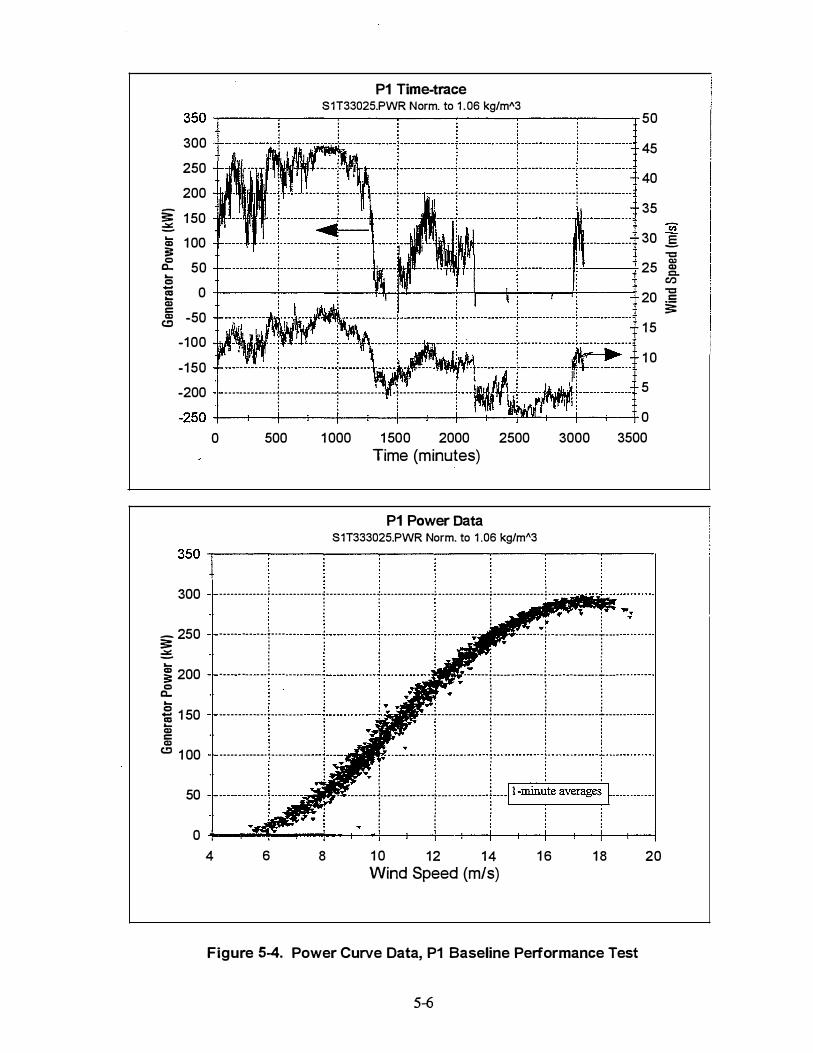
P1 Time-trace S1T33025.PWR Norm. to 1 .06 kg/ml\3

350 �----�----�----�----�----�------------.

300 +--··-----

250

200

;: 1 50 = � 1 00 :: g:_ 50 ... c

. . -!------1----- _ _ _ ,. - .................................. :- - - - - - - - - -..... ..... : ....... -------

. .

� 0 +-------�----�---4��----�-4--��--��----1 Q) c � -50

-1 00 -l!.AI!-1\!A.&.ITII� · -��FJI- -�L--· -- - -�----·'If�· · - - · ·· -•- - ·

-1 50

-200 . . . . . .

- - --- - - - - -- - - -:--............. - - - - - - --:--- .. - - · - - · - -ll· !- - - · ___________ ,.--·ill . .

-250 +-�--�--��--+--+--+--+--;-��-r--r-�--+

50

45

40

35

30

25

20

1 5

1 0

5

0 0 500 1 000 1 500 2000 2500

Time (minutes) 3000 3500

P1 Power Data S1T333025.PWR Norm. to 1 .06 kg/ml\3

350 �----�----�----�--�----�----�----�----,

300

- 250 == = ... 3 200 c

c..

.s 1 50 cc .... Q) c Q)

CJ 1 00

50

. . - - - - - - - - - - - - - .:. - - - - - - - - - -- - - -1· - - - - - - - - - - - - -�- - - - - - - - - - - - - - -!. - - - - - - - - - - - · - -t· · - -... - - - - - - - - -;- - - - - -

::::·

.::· ·

: r_: :: :�I:�: :: :: :r: .�-�-�- -

·

- · - - · - - ·

_

-

_

-:.:_

.

___ i ____

.. _ _

-

_

-

_

·

_

·

_

--

_

-

_

·

__

-

;: .. ::-. :�:�::�-............................ ................. . ...

- - - - - ............................. ............ ..

. . . . . . . . . . . . . . . . . . . . . J: _ _ ,,; _ _ _ ,, _ _ _ _ _ _ _ _ .... ! ........................... ! ............................ .!.. ......... ..

:

·- - - - - - - -t - · - - · - - · - - · - -r- - - - - - - · - - ·r- · - - · - - · - - - ·t- - · - · - - · - - · - -

.. .. l . ...

. .. T .. .. ... -H �--:te averng� �- --0 +-�--��--��--r--r-4--��--�-+--+--r��

4 6 8 1 0 12 14 Wind Speed (m/s)

1 6 1 8

Figure 5-4. Power Curve Data, P1 Baseline Performance Test

5-6

20

� ..§. "'C

Q)

Q) c..

CI'J "'C c §:

All Data Norm to 1 .06 kg/m"3 300 .---�--��--�.-,r-�.----�--�--�----�--� 500

. . \ I \ \ ..:..... . . . ' I \ . .,.. . . . : ; .... --. : 1\ : : : : ---------+- - · - -tf--------7{- · - - - - -¥1\--------+ · - · - -+---------+· - - · - - · -+-- -------

; I : " : \ / � \ . : : : : I : f : • � : : : : 250

400

_ 200 �

i • j I \ \. I f j Adjusted for terrain effects. ----------;- ·t· - - · - - ·;-----}-----;- - - - - ·1lJ\- -;-- --\·---:· - - Waked directions are removed. : I ! I : '

� \ ! "" . . . !11 l // t< /f. � ''}(. \\ l l j c

300 � .... CD 1 1 50

. . t � '\ ; ' . . . ----------]· · - - · - - · - ---r--ri -----:- - · - - · - -j- ,---------r· - -";y· · -:--... ----j-----·------r---------

CD c.. tl) CD 'S E

CD -tl) >-

1! / J : i \ j \" ! j j c

200 � 0

(/) 1 00 " : j I : � : "!\ : : :

-------h- · - - · - -it-r·- -l- - · - - · - - · - - 1- - - - -\· -+- - · - - · -_\l--------+ · - - · - - · -+---------- =to::

{ : r -- � : : \ : : " ...... -\ : : J lt �.: ; ; � ; ; \ \ ; ; 1 00 -/. ..,; . : : :i : �-'-L : ----,;r;--z· · ! ----------r· - - · - - · - ·r·------- !,- - - - - - - - ·r·-----t�-·--r·-------

• ]0 : : . : \ : : \ \ : 50

: : : " : : \ \ : : : .... : : � 0 +-��--+-�-r�--�+-�-+�--��-+��0

4 6 8 1 0 1 2 1 4 1 6 Wind S peed (m/s)

1 8 20

-- File #01 (55.0 hrs) -- File #02 (62.6 hi'S) --- File #05 (52.2 hrs)

Annual Average P1 Baseline P1 Baseline P1 Baseline Wind Speed File #01 File #02 Variation File #05

(m/s) (moh) AEP (kWh) AEP (kWh) (%) AEP (kWh) 5.3 1 2 236 955 250 860 5.87 205 877 5.7 1 3 305 494 320 899 5.04 273 537 6.2 1 4 377 733 395 405 4.68 346 217 6.6 1 5 451 869 473 049 4.69 422 606 7.1 1 6 526 1 02 552 127 4.95 500 477 7.5 1 7 597 068 630 380 5.58 576 705 7.9 1 8 663 1 65 706 327 6.51 649 506 8.4 1 9 724 733 779 444 7.55 71 8 629

22

Variation (%)

-1 3 . 12 -1 0.46 -8.34 -6.48 -4.87 -3.41 -2.06 -0.84

Note: All percent variations are calculated relative to P1 baseline file #01 .

Figure 5-5. Repeatability of P1 Baseline Power Curve, 50 Hour Data Sets

5-7

All Data Norm to 1 .06 kgfmA3

300 �------------------. ----.-��--------------�2000 : _,.. ..... �""- 1 \

250

_ 200 �

,_ Cl)

: : T � ....._. � ' ;,-'{ : __________ ; ........... ; ..... .;.-:.��-::..��------------;. _ _ _ :-:_ .; __ \ ________ ; _ _ _ _ _ _ _ _ _ _ _ �--

: i I ! i ! ' i \ i i . . . .\ . . \ . . : : I I : : \ : : : : \ i j I : i : : \ : :

----------i- - - - - - - - - -).-------y- -:�- - - - - - - - - - -+- - ---��- - - - - - -f------\----�- - - - - - - - - - -�- - -: ______ _ : tt : I : : : \ : \ : : l I l : l \ l l l i I i I i : i � i \ i i

1 500

c iii ,_ Cl) c. .,. � 1 50 "- - - - - - - · ·tt- · - - - - · i-1-- - - - - - -(- - - - - · ·t· · - - - - - - - - -(· · - - -\- - - - - - - - -\- - - - - - · ·iJ:· · - - - - - - 1 000 �

E .s � CIJ 1 00

50

. I :; . . . . � Jlii"!"'" : / . : : :\ ! \ : v f. : : : : : \ : ---------7:------.. -/. j -- --- -. ---i----- - -- -- -+--- - - - ---- ·t· · - - -- -- - --; --\-----j -- -•'\ .. ----+ ----------. : / : : : : : "\ : 'I( � I : I : . . . . \ : \ : 1 1 1 ; Adjusted for terrain effects. 'J \ 1

- - - -T- ·fT _ _ _ _ _ ·j·· - - - - - - - - Waked directions are removed. - - - - - · ·f'\.· - - - --'-::- - - - - - - - - - -

1 I . i "'. f' � ,.. : : " : " . / . : � '

500

.,. : : . ----..._ ...

0 +-�-+_,--+-��-+��4-�-+��+-�� 0 4 6 8 1 0 1 2 1 4 1 6

Wind Speed (m/s) 1 8 20

-- Files #01-06 (306.7 hrs) _,._ Files #07-13 (360.2 hrs)

Annual Average. P1 Baseline P1 Baseline Wind Speed Files #01-06 Files #07-13 Variation

(m/s) (mph) AEP (kWh) AEP (kWh) (%) 5.3 12 235 551 232 291 -1 .38 5.7 1 3 304 826 301 621 -1 .05 6.2 14 378 965 375 884 -0.81 6.6 1 5 456 998 454 1 44 -0.62 7. 1 1 6 537 169 534 650 -0.47 7.5 1 7 617 470 6 15 447 -0.33 7.9 1 8 696 870 695 574 -0.1 9 8.4 1 9 774 291 773 874 -0.05

22

c :g -Q '1:1::

Figure 5-6. Repeatability of P1 Baseline Power Curve, 300 Hour Data Sets

5-8

With this degree of repeatability, the power curves of Figure 5-6 were considered to be a highconfidence measure of the baseline P1 performance.

5 .4 P 1 with VG Configuration #1

VG Configuration #1 was installed on the P1 rotor blades on September 7, 1995. The configuration design was discussed in Section 4.5 and the array parameters are summarized in Table 5-1 . The P1 rotor had been lowered for maintenance, so the installation work was done at ground level. Tapetemplates were used for positioning, and the VGs were glued to the blade surface per the instructions of reference 13.

Table 5-1 . Array Parameters for VG Configuration #1 VG type Flat-plate vane, with leading-edge radius VG height 6.35 mm (0.25 in) VG length 25.4 mm (1 .0 in) VG angle of attack 15° nominal Lateral array spacing 9.52 em (3 .75 in) Spanwise extent of array Blade root to 57.5 % radius Chordwise location of array Variable, from 10% to 45 % chord Number of VGs in Array 69 per blade (138 total)

5.4. 1 Effect on Power Curve

After the P1 rotor was reinstalled, performance data were again recorded. Power curve data were collected between the dates of September 18, 1995 and December 18 , 1995, and site personnel observed that the blades remained unsoiled during this time period. Appendix A documents the powercurve files collected and the selection of valid data sets . Prior to binning, data sets were assembled and stored with file names 'vgcrun##.txt', where ## ranged from 01 to 08.

Figure 5-7 shows the measured power curves for P1 with VG Confiiuration #1, where the data have been grouped into two curves of approximately 300 hours each. The 300 hour curves with VGs show good repeatability with each other, although not as good as for the baseline P l . For most wind-speed bins the power output varies by less than 3 % , and the AEP variation is less than 2 % for all Rayleigh wind-speed averages over 6.2 rnfs (14 mph).

The 300-hour power were considered to accurately reflect the effect of VG Configuration #1 on P l performance. Figure 5-8 shows P1 performance with and without VGs. The curves show a noticeable drop in power output for wind speeds below 1 1 rnfs (25 mph) and an increase in power above this wind speed.

Table 5-2 shows the impact of the VGs in terms of percentage change in power output. The maximum increase in power was just over 4% at 12.8 rnfs (29 mph). The increase in peak rotor power was minimal, about 1 % at 17.2 rnfs (39 mph). From this standpoint, the design goal of increasing power at moderate wind speeds without increasing rotor peak power was met. However, the AEP table in Figure 5-8 shows that the losses at low wind speeds were not sufficiently offset by performance gains at moderate wind speeds and that the net effect of VG configuration #1 was a loss in AEP for annual average wind-speeds up to 8.4 rnfs (19 mph).

5-9

All Data Norm to 1 .06 kg/m"3 300 .---�----�--�--�----�--�--�----�--� 2500

250 . . . . . . . . . . ' .� . ...... ... ..... - .... ... .. ... .... ... .... -- � 4-- ........ ------ ---· ......................... ------ --· - .. .. ....... -- ............. -·-------- -- .. - - · --· --- - ----

• • • • 0 • •

: : : ,.... � -. : : : : : ..... : : : : : : . ' / � . / . . . . . : : >!( : \ : : : :

2000

c: _ 20 0 �

.... <D

---··-----i- - - - - - - - - -J--- -r--�---i- - -"'· · - - - - -L _______ lf_;_ _ _________ J ___________ ) _ _ _ _ _ _ _ _ _ _ _ _ L----------: � � r � \ ; \ � � � -'- v . : � . : : 1 500 �

� 1 50 E <D -., >

en 1 00

50

'I' • '\ • •

: I /: : '>!: -.. l \ : l l - - - - - - - - - -l- - -7/r· - - - - - - -T- - - - - - · ·r'>�-�:P��,-:---------�- - - - - - - · - -r·--------

� 1 I i : i i \\ )\ i i . I . . . . . . . - - - - - - - - -.; -. t-r-. - - .; -------- -· -!---. --.--.-.; ---.----- .. ; . . --- ·\· .; --,-------�---.-- - - - - -.; -----·-----

: If : : : : � \ : : v 1 1 : :... \ : : f. l : : \ : -------·y-f· - - - - - · - �------ Adjusted for terrain effects. ----\�'.-;------------�-----·-----

/ f: ' Waked directions are removed.

Ill. f..'- : I llll : "- : 'I;. •

c.. ., s :::1 c:

1 000 � ::tt::

500

:/ : l"' '-... "-ci 0-+-��__,,__+--t--+---t-+--+--+--+--+-+---t---+-':::oo;-__..,=--t O

4 6 8 1 0 1 2 1 4 1 6 Wind Speed (m/s)

1 8 20 22

-- VG Input Files #01 -04 (299.5 hrs) -- VG Input Files #05-08 (302.4 hrs)

Annual Average P1 with VGs P1 with VGs Wind Speed Files #01-06 Files #07-1 3 Variation

(m/s) (mph) AEP (kWh) AEP (kWh) 1%l 5.3 1 2 220 61 1 227 804 3.26 5.7 1 3 289 848 297_,_41 1 2.61 6.2 1 4 364 706 372.363 2.1 0 6.6 1 5 444,1 62 451_,_656 1 .69 7.1 1 6 526 258 533 394 1 .36 7.5 1 7 608,926 61 5 51 0 1 .08 7.9 1 8 691 068 696 940 0.85 8.4 1 9 771 ,437 776_,_493 0.66

Figure 5-7. Repeatability of P1 Power Curve with VGs, 300 Hour Data Sets

5-10

All Data Norm to 1 .06 kgfmA3 300 ..,-----,-----,--,--,..---..,----,,..----,---o--.,----. 4000

250

_ 200 � .... Q) � 1 50 E Cl) -"' >

(f.) 1 00

5 0

0

4

• • • 0 • : : -- : � --..[ : .. --·- --- _]_ . -.. . -.... )L. ---.. I. .. .. -��-=···· _.J_ ..... . . . �-----------;- - · -- · - - . ---�---: ;/ I : : � : : :

� 1: .,.. � � \ � � � : 1 : I : i -.; i � i i i -- ....•••• ;- . • . . . . . -J . . L-.!. ...... : --· ······--;_ - -------�---.. -.... -:,1.. --- •...... L .. --·-.. ---�----------

: f : I : . ' \ : "l : : 1 1 'I l : l -.: l \ l l . j · . . ' '\ · \ . ...... . i I � i l i '- l \ i ..,... i ----------1-··-· i- · /:------------! --·- -- · -··t -----------:· ·--·---\-r------� ---1·-·--····--·:- ----------

� I I � : l � � \ � � i ;I i : i i \ \ l l -----·····y1·· -.-- .... t·------ - ., ...... -- .. ·j······ ---··t ....... ····t·-\" ----r � � . ... . . 't ----------: ; ; ; ; � ; � ; ... ..... ,;. ........ : : : -�--------"·i- - - - - · -\-- - ·�-----------

1; ; Adjusted for terrain effects. ; 'i \ ; 1 ! Waked directions are removed. ! ; '-..-.:. "'j '-..

3000

2000

1 000

rl . : . � .... : ; '-,.0

6 8 1 0 1 2 1 4 1 6 Wind Speed (m/s)

1 8 20 22

-- Baseline P1 (667 hrs) _.,._ P1 with VG Config. #1 (602 hrs}

Annual Average P1 @ 288 kW P1 with VG Wind Speed Baseline Configuration #1 Variation

(m/s) (mph) AEP (kWh) AEP (kWh) (%) 5.3 1 2 234 829 224 737 -4.30 5.7 1 3 304 1 29 294,1 82 -3.27 6.2 1 4 378 314 369 090 -2.44 6.6 1 5 456 466 448,445 -1 .76 7.1 1 6 536 844 530 322 -1 .21 7.5 1 7 61 7 494 6 12,641 -0.79 7.9 1 8 697 459 694 31 7 -0.45 8.4 1 9 775 587 774,1 43 -0. 1 9

Figure 5-8. Effect of VG Configuration #1 o n P 1 Performance

5-1 1

c: i::ij .... Cl) c. "' � :::> c: :E -0

"'t:

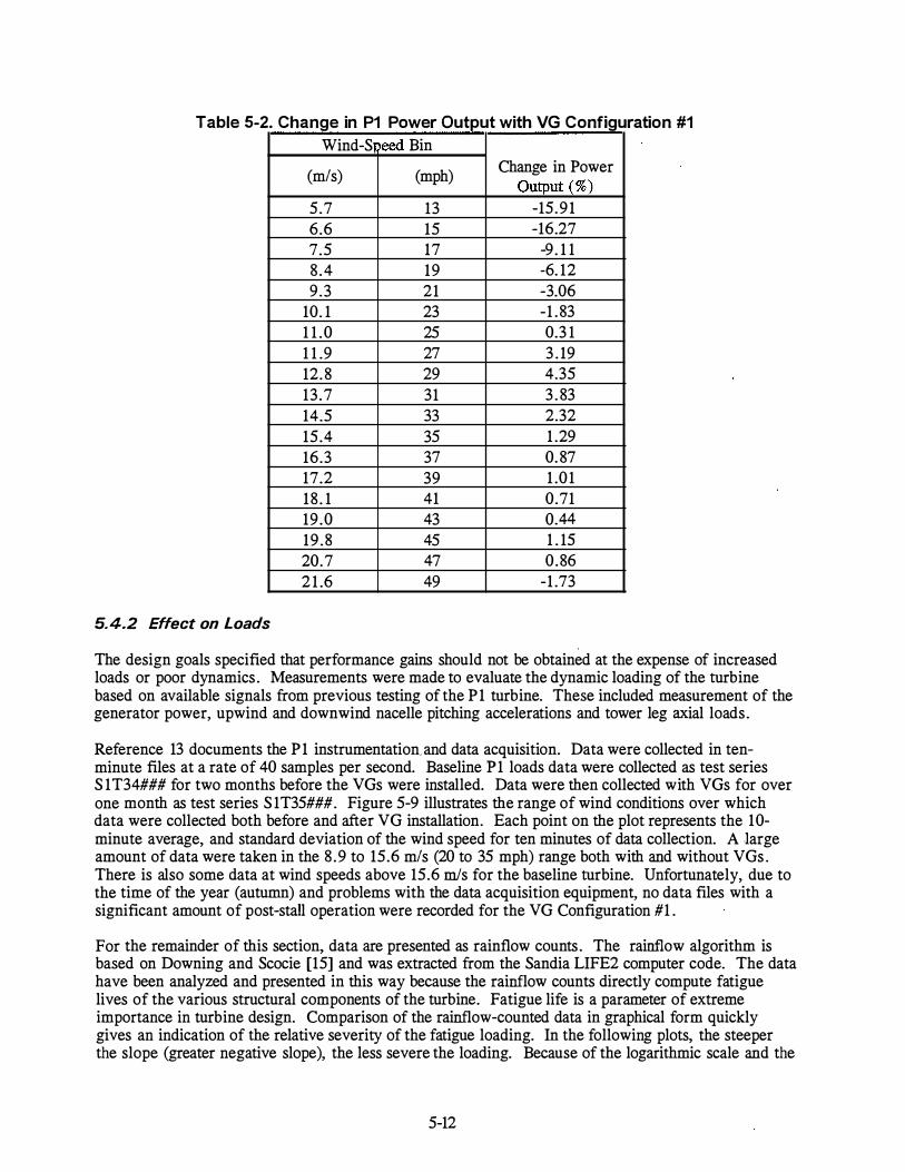
Table 5-2. Change in P1 Power Output with VG Configuration #1

Wind-S peed Bin

(mls) (mph) Change in Power

Output (%)

5.7 13 -15.91 6.6 15 -16.27 7.5 17 -9. 1 1 8 .4 19 -6. 12 9.3 21 -3.06

10. 1 23 -1 .83 1 1 .0 25 0.3 1 1 1 .9 27 3 . 19 12.8 29 4.35

13 .7 31 3 . 83 14.5 33 2.32 15.4 35 1 .29 16.3 37 0.87 17.2 39 1 .01 18 . 1 41 0.71 19 .0 43 0.44

19 .8 45 1 . 15 20.7 47 0.86

2 1 .6 49 -1 .73

5.4.2 Effect on Loads

The design goals specified that performance gains should not be obtained at the expense of increased loads or poor dynamics. Measurements were made to evaluate the dynamic loading of the turbine based on available signals from previous testing of the P1 turbine. These included measurement of the generator power, upwind and downwind nacelle pitching accelerations and tower leg axial loads.

Reference 13 documents the P1 instrumentation.and data acquisition. Data were collected in tenminute files at a rate of 40 samples per second. Baseline P1 loads data were collected as test series S 1 T34### for two months before the VGs were installed. Data were then collected with VGs for over one month as test series S 1 T35###. Figure 5-9 illustrates the range of wind conditions over which data were collected both before and after VG installation. Each point on the plot represents the 10-minute average, and standard deviation of the wind speed for ten minutes of data collection. A large amount of data were taken in the 8 .9 to 15.6 mls (20 to 35 mph) range both with and without VGs . There is also some data at wind speeds above 15.6 m/s for the baseline turbine. Unfortunately, due to the time of the year (autumn) and problems with the data acquisition equipment, no data files with a significant amount of post-stall operation were recorded for the VG Configuration #1 .

For the remainder of this section, data are presented as rainflow counts. The rainflow algorithm is based on Downing and Scocie [15] and was extracted from the Sandia LIFE2 computer code. The data have been analyzed and presented in this way because the rainflow counts directly compute fatigue lives of the various structural components of the turbine. Fatigue life is a parameter of extreme importance in turbine design. Comparison of the rainflow-counted data in graphical form quickly gives an indication of the relative severity of the fatigue loading. In the following plots, the steeper the slope (greater negative slope), the less severe the loading. Because of the logarithmic scale and the

5-12

fact that material fatigue characteristics are non-linear, small changes in the rainflow counts can cause large changes in turbine fatigue lives.

-(J) -:;§! -

z 0 � > w Cl Cl c: <( Cl z g (!j > <( z :;§! 0 ,....

3

2.5

2

1 .5

1

0.5

f-·

AWT-26 P1 VORTEX GENERATOR TEST - LOADS DATA COLLECTION - WIND DISTRIBUTION

!--··

r- i o . I I

0 2 4 6 8 1 0 1 2 1 4 1 6 1 8 1 0 MINUTE AVG WIND SPEED (M/S)

20

Figure 5-9. 1 0-Minute Average Wind Speeds during P1 Loads Measurement

5-13

The P 1 turbine· has a dynamic mode that includes a pitching motion of the nacelle. Several

configuration changes were made to address this problem and minimize this mode, but it is still of some concern. During the VG testing, nacelle pitching accelerations were measured at both the upwind and downwind ends of the nacelle. Figure 5-10 shows the rainflow counts of upwind and downwind nacelle accelerations for the full data sets, both with and without VGs. The plot shows that the downwind accelerations were slightly more vigorous with VGs. On the other hand, the upwind accelerations with no VGs are much more vigorous than with VGs. This is most likely due to the fact that there is significantly more amount of post-stall operation (wind speed greater than 15.6 m/s) represented in the baseline data and very little in the VG data.

Figure 5-1 1 attempts to present a better comparison by including only data collected with ten-minute wind speeds between 8.9 and 15.6 m/s. In this plot, it is seen that the downwind accelerations with VGs are significantly more vigorous than without VGs. However, the upwind accelerations without VGs are still somewhat more vigorous than with VGs. This is possibly due to differences in atmospheric turbulence between the various data files, but the exact explanation is not clear.

The plot of the rainflow counts of generator power output, and thus drivetrain torque, appears in Figure 5-12. Three curves are shown: all baseline data, baseline with wind speeds 8.9 to 15.6 m/s only, and with VG Configuration # 1 . It is fairly clear that the generator power output oscillates more, and most likely reaches higher peaks, with the VGs installed. The data with VGs compare to the data without VGs at a much higher average wind speed containing significantly more post stall operation.

The data in Figure 5-13 show rainflow counts of tower leg axial load, and is a bit more difficult to interpret. Again, three curves are presented: all baseline data, baseline 8 .9 and 15.6 m/s only, and with VGs. The VG results are higher than the baseline data at the left- and right-hand ends of the curve. However, in the body of the curve the VG data are well below the baseline at both the comparable and higher wind speeds. Data towards the right on the curve have more impact because the loads are higher. Thus, in the most important part of the curve the VG data do show higher than the baseline. It should also be noted that these results depend somewhat on absolute yaw position, a signal that was not available during these tests . If the wind was from a different direction, the results from a given tower leg would be somewhat different.

Overall, it appears that the dynamic response of the turbine as represented by rainflow counts of fatigue cycles was increased by the presence of vortex generators. The data indicate that the increase is slight to moderate. However, if more post stall data were collected, the increase in dynamic response could become more pronounced.

It should also be noted that the data set is not large and that changes in atmospheric conditions could have a similar level of impact. The data should be interpreted with caution and an understanding of its uncertainties and limitations. If the use of VGs were pursued, these data would be used to analyze the relative impact (on turbine fatigue) of vortex generators in order to understand the economic tradeoffs between improved power performance and decreased turbine fatigue life.

5-14

0 z 0 () w (f) CJ z � a: w 0.. 0 (jj w _J () b

i I

��==r-=��--�----�----�----�----- 1 1 UPWIND PTICHING NO VG'S ALL DATA

I I

I �------�----�--·--�

� ��TCHING t---�

+� . S1 T35001 -<l39 l i

3 DOWNWIND � , L • 1 -F : + ++ -i-f+ 1 l � cP - * - . .. � -+;..f:t- + 1 E-04:::----iNO VG'S ; � 111!:!11 * I - : •

·t-+--- , LL DATA � � *Ill-;� • � - � 1a1++- j

� l D O l l l 1 E-05+-----r-----ri ----,1-----+1 -----+i -----:r: ----�.

0 0.5 1 1 .5 2 2.5 3 3.5 PEAK-PEAK ACCELERATION (G'S)

Figure 5-10. Nacelle Pitch Accelerations, Full Data Sets

Figure 5-1 1 . Nacelle Pitch Accelerations, Wind Speeds between 8.9 and 1 5.6 m/s

5-15

1 E+OO�----�------�----�------�------�----�

0 z 0 () w (/) CJ z � c: w 0.. 0 -(/) w _J () >()

1 E-02::!----+-=::=:;:::-..li�-+--------1 NO VG'S ALL DATA

WITH VG/S

• - ·

• * * r ** *

1 E-05+------+------,_----�------�------�----� 0 50 1 00 1 50 200 250 300

PEAK-PEAK POWER (kW)

Figure 5-1 2. P1 Generator Power Output, Rainflow Cycle Counts

1 E+0 1 �------------------�----------�--------------

� 1 E+OO;��----- --�---�----�-----�----------�------o : • • i : . . I () - '· i � 1 E-01 '*.. . NO VG;S CJ . � ;1f:• l ALL DATA z I *•+ i . - - ! "'•::t-+4- j_ i � i �* : ,+..�- .r , 0: 1 E-02� • , - '""' "+ . . � -,�:::ti:�++ I 1 0 ' ·· -� ++ i 0) 1 E-03=�----�----��----�� --�-� .• �.�.� •• -.--�i ------�----� W WITH VG'S ,1 · · · · - · -• :bi _J i I = = • ·�o. •• () _ 9-1 6 m/s 1 , = r""• b 1 E-04�J-------l---====;:=---INO VG'S I : � **l +..,... - .

= 9-1 6 M/S � fE *++ .. 11!1 DATA ONLY 1 I ,,.. * '""' i - i 1 = " '" I ++

1 E-05�----+-----+---��==�� ----�i ----�:----� 0 50 1 00 1 50 200 250

P EAK-PEAK LEG LOAD (k. N) 300

Figure 5-13. P1 Tower Leg Axial Load, Rainflow Cycle Counts

5-16

350

5.4. 3 Analysis I Suggested Improvements to Configuration

As shown in Figure 5-8, VG Configuration #1 achieved the desired performance above 1 1 m/s (25 mph). Power output was increased at moderate wind speeds and the slight increase in peak power indicates that the VG array had become largely stalled by wind speeds above 17 m/s (38 mph). This indicates that the array was placed as far forward on the blade as possible while still allowing the blade to retain its baseline stall behavior.

Below 1 1 m/s, VG drag penalties led to a loss in turbine performance. The measured drag loss in performance was generally greater than that predicted by PROPPC calculations. It appears that the 3-D turbine blade did not experience the same amount of lift augmentation as was measured in the wind tunnel for the 2-D airfoil sections, but it did experience significant drag penalties. Moving the VGs aft on the airfoil would decrease the amount of drag penalty, but would also cause the VGs to be less persistent. Therefore, decreasing drag losses by moving the VGs aft would likely compromise some of the performance gains above 1 1 m/s. A similar logic could be applied to either making the VG array less dense or using smaller VGs.

To evaluate the potential for improving VG Configuration #1, an annual energy calculation was performed for the power curve of Figure 5-8 assuming no drag losses below 1 1 m/s and retaining all of the performance gains above 1 1 m/s. Table 5-3 shows resulting performance gains of less than 15% for all wind-speed average of 8.4 rnfs and below. This confirms that the effectiveness of the VGs on the 3-D blade was less than that measured for the 2-D airfoil sections. Based on these results, field testing of a second VG configuration was not deemed worthwhile.

Table 5-3. Potential for Improved Performance of VG Confi guration #1

Rayleigh Annual P1 Baseline P1 with 'Ideal' (no drag loss) Average Wind Speed Power Curve VG Configuration #1 Variation

AEP ( kWh) AEP (kWh) (%)

5.3 m/s (12 mph) 234,829 236,412 0.67 5. 7 m/s (13 mph) 304, 129 306,817 0.88 6.2 mls (14 mph) 378,3 14 382,329 1 .06 6.6 m/s (15 mph) 456,466 461 ,972 1 .21 7. 1 m/s (16 mph) 536, 844 543,905 1 .32 7.5 rrl!s (17 mph) 617,494 626,087 1 .39 7.9 m/s (18 mph) 697,459 707,498 1 .44 8.4 m/s (19 mph) 775,587 786,964 1 .47

As the field test results showed a negative net impact on AEP, no rigorous calculations were performed to evaluate the effect on cost of energy (COE). The materials necessary for one prototype VG array, including the VGs and the tape-templates which were used to locate them for installation, were purchased for about $200. With the rotor on the ground the installation process took about 6 manhours, including the time required to mark reference lines on the rotor, the attachment and removal of the tape templates and the attachment of the VGs themselves. The installation procedures were designed so that they could be completed from a man-basket on a crane, but this would significantly increase the time and expense required for the installation.

5-17

6.0 Results and Conclusions

A rigorous investigation has been completed of the use of vortex generators to augment performance of the stall-regulated A WT-26 wind turbine. A VG array was designed which led to increased power output at moderate wind speeds and a negligible effect on peak rotor power. However, VG drag penalties caused a loss in power output at low wind speeds, and the net effect of the VG array was a decrease in annual energy production for sites with average wind speeds up to 8.5 rnfs (19 mph). Analysis indicated that design modifications to reduce the drag losses would also be likely to reduce the performance benefits at higher wind speeds. For the 3-D turbine blade, it appears that the VGs caused lift increases that were smaller than those measured for the 2-D airfoil sections.

The impact on loads was less conclusive. The available data indicated that the VG array caused an increase in dynamic loads, but the data sets were somewhat limited. Had the performance of the VG design been more promising, further measurements would have been warranted to better quantify the effects on loads and component fatigue life.

While the present work did not lead to improved AEP for the A WT-26 turbine, it does contribute to the understanding of performance augmentation of wind turbines with VGs. Wind tunnel measurements have quantified the effect of VGs on NREL S-series airfoils for a wide range of VG design parameters. The safe design of a VG array for a stall-regulated turbine has been demonstrated, and several issues involving optimal performance with VGs have been identified and addressed.

6- 1

7.0 Referen ces

1 . Tangier, J .L., HAwr Performance Prediction Code for Personal Computers, Solar Energy Research Institute, January 1987.

2 . Sullivan, T.I., Effect of Vortex Generators on the Power Conversion Performance and Structural Dynamics Loads of the MOD-2 Wind Turbine, NASA TM, 83680, 1984.

3 . Gyatt, G. W. , Development and Testing of Vortex Generators for Small Horizontal Axis Wind Turbines, AeroVironment Inc. , NASA CR-179514, July 1986.

4. Quinlan, P.J., Scheffler, R.L. , and Wehrey, M.C. , Performance Test Results of Vortex Generators Attached to a Vertical Axis Wind Turbine, 7th ASME Wind Energy Symposium, January 1988.

5 . Haller, M.E., Vortex Generator Field Tests on ESI 54 WIGs (modified), an Empirical Approach, Sea West Altamont, Inc . , July, 1990.

6 . UWAL Report 1523, University of Washington Aeronautical Laboratory, June 1996.

7 . UWAL Report 396-F, University of Washington Aeronautical Laboratory, March 1995.

8 . Allen, H.J., and Vincenti, W.G., Wall Interference in a Two-Dimensional Flow Wind Tunnel, with Consideration of Compressibility, NACA Report No. 782, 1944.

9 . Hoffmann, M.J . , Ramsay, R.R. , Gregorek, G . M. , Unsteady Aerodynamic Performance of lVznd Turbine Airfoils, Windpower '94 Proceedings, American Wind Energy Association, May 1994.

10. Hoerner, S.F. Fluid Dynamic Drag, Library on Congress Ca�og Card Number 64-19666, 1965 .

1 1 . Ramsay, R.R. , Hoffmann, G.M., and Gregorek, G.M. , Effects of Grit Roughness and Pitch Oscillations on the S815 Airfoil, Midwest Research Institute Contract Number XF-1 1009-3, August, 1994.

12. Eppler calculations by private corresponde:nce with Jim Tangier [need to call Jim about this]

13 . Vortex Generators Test Plan, AWT Report TP260009, August, 1995.

14 . A WF-27 Power Curve Design Book DB2 73011 , April 1996.

15 . Downing, S .D. , and Socie, D. F., Simple Rainflow Counting Algorithms, International Journal of Fatigue, January 1982.

7- 1

APPENDIX A

SUM:MARY DATA SET LOGS (Actual data collected under this program is Protected Wind Technology Data)

Original Filename

s 1 t35027 . raw

s 1 t35028.raw s 1 t35029. raw

s l t35030.raw

s l t3503 l .raw

s l t35032.raw

� -

s 1 t35033 . raw

s 1 t35034 .raw s l t35035 . raw s 1 t35036.raw

s l t35037. raw

s I t35038.raw

Summary Data Log I Valid Data Sets for Pl Power Curve with VGs

Test -Segment Minutes Filename Start - Stop

vgseg06 l .txt 32 1 - 499 vgseg062. txt 55 1 - 738 vgseg063 . txt 1 538 - 1 840

NA NA vgseg064.txt 1 079 - 1 769 vgseg065. txt 1 866 - 2 1 07 vgseg066.txt 27 16 - 28 1 9 vgseg067. txt 2 - 89 vgseg068.txt 200 - 2061 vgseg069 . txt 2 - 247 vgseg070.txt 1 083 - 1 585 vgseg07 1 .txt 1 97 - 308 vgseg072.txt 357 - 443 vgseg073 . txt 600 - 1 1 36 vgseg074.txt 1 195 - 1 494 vgseg075. txt 1 5 8 1 - 230 1 vgseg076.txt 2 - 9 1 3 vgseg077. txt 1 434 - 2493

NA NA vgseg078 . txt 1 529 - 1 737 vgseg079.txt 265 - 535 vgseg080.txt 586 - 727 vgseg08 1 .txt 2834 - 3 1 1 1 vgseg082.txt 47 - 533 vgseg083 . txt 939 - 1 329 vgseg084. txt 1 525 - 1604 vgseg085 . txt 1 687 - 1 75 1 vgseg086.txt 23 1 4 - 257 1 v�087.txt 2666 - 300 1

NA NA

Total Minutes

1 79 1 88 303 NA 69 1 242 1 04 88

1 862 246 1 04 1 1 2 87

537 300 72 1 9 1 2 1 060 NA 209 27 1 1 42 278 487 391

. -

------80 65

258 336 NA

crunp l . in Filename

vgcrun06. txt "

"

NA vgcrun06. txt

"

"

vgcnm07. txt "

"

"

"

"

"

"

"

vgcrun08.txt "

NA vgcrun08 . txt

"

"

"

"

"

"

"

"

"

NA -- ··-�·----·-- --- -·-----

Notes I Conditions

No run time

No run time

Lar�catter =:> l£!!1_g ---.� ------�---

1 I

> t0

Original Filename

s l t350 17 .raw " " " "

s l t350 1 8 .raw s l t350 1 9.raw

" "

s 1 t35020.raw s 1 t3502 1 . raw

"

" " "

s 1 t35022. raw s 1 t35023. raw

"

"

s 1 t35024.raw s l t35025. raw

" " " "

"

"

s 1 t35026. raw "

"

s 1 t35027. raw

Summary Data Log I Valid Data Sets for 1,1 Power Curve with VGs

Test-Segment Filename

vgseg030.txt vgseg03 1 . txt vgseg032.txt vgseg033 .txt vgseg034 . txt vgseg035 .txt vgseg036. txt vgseg037. txt vgseg038 . txt vgseg039 .txt vgseg040.txt vgseg04 l .txt vgseg042. txt vgseg043 . txt vgseg044. txt vgseg045.txt vgseg046.txt vgseg047 .txt vgseg048. txt vgseg049. txt vgseg050. txt vgseg05 1 .txt vgseg052.txt v��053.txt vgseg054.txt vgseg055 .txt vgseg056.txt vgseg057.txt vgseg058 .txt vg�eg059. txt vgseg060. tx t

Minutes Total crunp l . in Start - Stop Minutes Filename

2 - 356 355 vgcrun04.txt 559 - 699 1 4 1 "

873 - 952 80 "

1 5 1 1 - 1 854 344 "

2073 - 2 1 53 80 "

2901 - 3024 124 "

1 94 - 399 206 "

6 1 2 - 864 253 "

1 1 1 1 - 1 9 1 9 809 "

2 - 1 043 1 042 vgcrun05. txt 2 - 125 1 24 "

240 - 64 1 402 "

95 1 - 1 046 96 "

1 222 - 1 308 87 "

3295 - 3382 88 "

2 - 2639 2638 "

1 983 - 2 1 40 1 5 8 "

-

2 1 8 1 - 2606 426 "

28 1 2 - 3004 1 93 "

1 904 - 2245 342 vgcrun06. txt 76 - 2 1 0 1 35 "

55 1 - 6 1 7 67 "

8 1 8 - 1 0 1 7 200 "

1 1 7 1 - 1254 84 "

1 329 - 1755 __ _1�L __

" ----

3 1 7 1 - 3276 1 06 " ---- ---- -------

3555 - 366 1 107 "

96 - 695 600 " --

1 1 37 - 1 524 388 "

-

T67o::t873___ --------264 - --- --- -----------..

-------

�--------- ·--·-·------·--- · · --······ - ---··--------- ·-----

2 - 2 17 2 1 6 "

�- --

Notes I Conditions

I

I -�

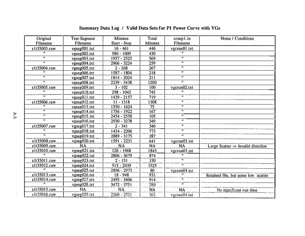
:> w

Original Filename

s l t35003 . raw " " "

s 1 t35004. raw " " "

s l t35005. raw " "

s I t35006. raw " " " "

s l t35007 .raw " "

s l t35008.raw s 1 t35009 . raw s l t350 1 0 . raw

"

s lt350 1 1 . raw s l t350 12 .raw

"

s l t350 1 3 . raw s l t350 1 4. raw

"

s I t350 1 5 . raw s l t350 16 . raw

Summary Data Log I Valid Data Sets for Pt Power Cm·ve with VGs

Test-Segment Minutes Filename Start - Stop

vgsegOO 1 . txt 1 6 - 46 1 vgseg002.txt 580 - 1 009 vgseg003. txt 1 957 - 2525 vgseg004.txt · 2966 - 3224 vgseg005. txt 2 - 268 vgseg006.txt 1 587 - 1 804 vgseg007.txt 1 8 1 4 - 2024 vgseg008.txt 2239 - 3438 vgseg009.txt 3 - 1 02 vgsegOl O. txt 298 - 1 042 vgseg0 1 l .txt 1 439 - 2 1 57 vgsegO 12 . txt 1 1 - 1 3 1 8 vgsegO 1 3 . txt 1 550 - 1 624 vgseg0 1 4.txt 1 756 - 1 922 vgsegO 1 5 . txt 2454 - 2558 vgseg01 6.txt 2930 - 3278 vgsegO 17 . txt 2 - 34 1 vgseg01 8 .txt 1 434 - 2206 vgsegO 1 9. txt 2889 - 3 1 75 vgseg020.txt 1 59 1 - 223 1

NA NA vgseg02 l .txt 1 26 - 1 968 vgseg022.txt 2806 - 3679 vgseg023 . txt 2 - 1 5 1 ---vgseg024.txt 5 1 5 - 2039

·-------------

v�g025 .txt 2896 - 2975 vgseg026.txt 1 8 - 948 vg�027.txt 2493 - 3406 v�g02��L- 3472 - 375 1 ·--- · --- - - --- - - - -

NA NA ·--

--

-

-

-··

vgscg029. txt 2260 - 252 1 .

Total Minutes

446 430 569 259

crunp 1 . in Filename

v_gfrunO 1_. txt " " "

.. . -

267 "

2 1 8 "

21 1 "

1200 "

1 00 vgcrun02.txt 745 "

7 1 9 " ------

1 308 "

75 "

1 67 "

1 05 "

349 "

340 "

773 " · --

287 --- ----64 1 NA 1 843 874 1 50

·---- ---

1525 -----------80 �-�-------·

93 1 9 1 4 ·-·---------· - · 280 ------- - - ....... - ---

-

- . . NA

------ ----- ------· 262

"

vgcrun03 . txt NA

vgcrun03 . txt " "

---· " -·--------· _.Y££!!!ll04 !!.&____ "

" · --------

" . ··- ··········-·-··-·-···--·--··-------

NA · ·- · ·---··--------- ----

vgcrun04 .txt

Notes I Conditions

Large Scatter =:> Inval id direction

Retained file1 but some low scatter

--------- --

___ __ I':!Q_�jg!!Wcant run time

j I I I i I j ! I

-·

!

j i

Original Filename

s 1 t33028.pwr s 1 t33029 .pwr s l t33030.pwr s 1 t3303 l .pwr s l t33032. pwr s l t33033.pwr

"

s 1 t33034. pwr slt33035.pwr slt33036.pwr slt33037.pwr

"

"

t s 1 t33038.Qwr "

"

s l t33039.pwr s 1 t33040. pwr s 1 t3304 l .pwr s l t33042.pwr s 1 t33043 .pwr s l t33044.pwr s l t33045. pwr s 1 t33046. pwr

"

s l t33047.pwr "

"

"

_ll.lQ304�!pwr _ll.H}J049..:Q�

"

Summary Data Log I Valid Data Sets for Pl Baseline Power Curve

. Test -Segment Minutes Total Filename Start - Stop Minutes

None NIA NIA None NIA NIA None NIA NIA None NIA NIA None NIA NIA

p 1 bsln27. txt 2 - 763 76 1 p l bsln28.txt 922 - 1 893 97 1

None NIA NIA None NIA NIA None NIA N/A

p l bsln29.txt 2 - 376 374 · --· p lbsln30.txt 1 326 - 1 609 283 p1bsln3 l . txt 234 1 - 2537 1 96 p 1bsln32.txt 455 - 1 990 1 536 p 1 bsln33. txt 2009 - 3263 1 255 p1 bsln34.txt 3339 - 3434 96 p 1 bsln35 .txt 2 - 27 1 4 27 1 3

_ p 1 bsln36. txt 2 - 1 1 65 . 1 1 64 None NIA N/A

p lbsln37.txt 1 1 0 - 3 1 25 30 1 6 p lbsln38.txt 386 - 3097 27 1 2

None N/A N/A p l bsln39. txt 2 - 1 93 1 1 930 p 1bsln40.txt 2 - 656 655 p 1 bsln4 1 .txt 1 1 77 - 2342 t 1 65 --- -----p 1 bsln42.txt 2 - 655 654 - --

-

---p lbsln43 .txt 1 1 77 - 2822 1646 p l bsln44.txt 2930 - 3054 125 ·--- -·

-

p l bsln45 .txt 3448 - 375 1 304 -·-·

-

--- -· None N/A N/A ·-

--

- - - ---·--- -·-····· . ·····----·--· --· ---··--

__ t�.!hs!!146:txt ___ 8 1 - 237 1 67

·

--

-

·

..

----- ·- · -·-· · · · ----- · ···- ·· ·· - - ·- ·· -· ·· -- -p l b s l n47 . t x t · 584 - 375 1 3 1 66

crunp l . in Notes I Conditions Filename

NIA Blade soiled with bugs NIA Blade soiled with bugs NIA Blade soiled w ith bugs NIA Blade soiled w ith bugs I NIA Blade soiled with bugs

p 1 crun06. txt Blade returned to dean condition "

N/A Blade icing N/A Blade icing N/A Blade Icing I

I?Jcrun06:txt

• "

"

p 1 crun07. txt Missing 608-665 " I ' " '

____£ 1 crun08 .txt Miss i!!g 1 53-2 1 4 " Some rain, but data OK

N/A Stormy conditions p 1 crun09.txt Missing 264-324 p 1 crun l O. txt Missing 552-604

N/A Snow ice p 1 crun 1 1 . txt Missing 1 59-220

"

" ·-· _J!!Cr!!!!.!2 .txt

"

"

"

N/A - ·--·-·-·-·· - --- - -- -·--- · --- . "

·

-

.

-

·

..

··- ---·--- ·--· ·

-

-

·

tD crun 1 3 . t x t

-

fy!�sing t 52-2 1 7

I�l!!g

--------��--�� Mi��it1g 745-805--

--

--·

> �

Original Filename

s l t330 1 1 .pwr s l t330 12 .pwr

"

"

s l t330 l 3 .pwr "

s l t330 1 4 .pwr s l t330 1 5.pwr s l t330 1 6.pwr

"

"

s l t330 1 8 .pwr "

"

"

s l t330 1 9.pwr s l t3302 1 .pwr

"

s l t33022.pwr s l t330 1 7.pwr

"

s l t33020.pwr s l t33023 .pwr

"

"

s l t33024. pwr s l t33025 .pwr

"

"

s l t33026.pwr s l t33027.pwr

S_ummaa·y nata Log I Valid Data Sets for PI Uaseline I,owea· Curve Test-Segment Minutes

Filename Start - Stop p 1 bsln0 1 . txt 1 - 1 050 p l bsln02.txt 1 - 677 p 1 bsln03 . txt 1 044 - 1 170 �1 bsln04.txt 1 698 - 1 945 p l bsln05. txt l - 1 450 p 1bsln06.txt 2 1 79 - 2434 p 1 bsln07. txt 1 25 - 1 434

None NIA p l bsln08. txt 1 - 788 p 1 bsln09 .txt 1 689 - 2986 p 1 bsln 1 0 . txt 3067 - 329 1 J) 1 bsln 1 l . txt 27 1 - 446 � 1 bsln 12 . txt 806 - 1 542 p 1 bsln 1 3 . txt 1603 - 3252 p l bsln 1 4. txt 3299 - 375 1

None NIA p 1 bsln 1 5 . txt 1 - 1 042 J!.!bslnt 6.txt 1 357 - 1 732 ----

p l bsln!7.txt 1 9 1 6 - 2466 p 1bsl n 1 8 . txt 2 - 6 1 3 p 1 bsln 1 9 . txt 1 554- 1 754

None NIA p 1 bsln20. txt 60 - 3 1 4 p t bsln2 1 . txt 1 383 - 1 5 1 3 �1 bsln22.txt 1 565 - 1 9 1 4 p 1 bsln23 .txt 2 - 1 004 p 1 bsln24.txt 2 - 1 397 p 1bsln25 .txt 1 5 1 0 - 2 1 49 p 1 bsln26.txt 2972 - 306 1

---�·

None NIA None NIA

Total M inutes

1 050 677 127 248 1 450 256 1 3 1 0 NIA 788 1 298 225 ---- -1 76 737 1 650 453 N/A 1 042 375 -- ----

550 6 1 1 200 NIA 254 1 30 349 ----1002 1 395 639 89

- .

-

crunp l . in Filename

� 1 crunO 1 . txt "

"

"

"

p l crun02. txt "

NIA p1 crun02.txt

"

p 1 crun03 . txt "

"

"

"

N/A _p_l crun04.txt

"

"

"

"

NIA p 1 crun04. txt

"

"

p l cnm05.txt "

"

"

·-------·- -----

N/A NIA -�-----····-

N/A N/A

Notes I Conditions

Large scatter, data not used

Icing, scatter, data not used

Icing scatter, data not used

File doesn't exist - numbering error Blade soiled with hug� -- ____ __

i '

REPORT DOCUM ENTATION PAGE I Form Approved OMB NO. 0704-0188 Public reporting burden for this collection of information is estimated to average 1 hour per response, including the time for reviewin� instructions, searching existing data sources, gathering and maintaining the data needed, and completing and reviewing the collection of information. Send comments regardit1fc t is burden estimate or any other as�ect of this collection of information, Including sug�estions for reducin� this burden, to Washington HeadWarter:s Services, Directorate for In o"(lation Op��tions and Reports, 12 5 Jefferson Davis Highway, Suite 1204, ArlinQton, A 22202-4302, an to the Office of Manaoement and udoet, Paperwork Reduction Project 0704-0188 , Washington, DC 20503. 1 . 2. REPORT DATE 3. REPORT TYPE AND DATES COVERED

December 1 996 Subcontractor Report, 1 995-1 996

4. TITLE AND SUBTITLE 5. FUNDING NUMBERS

Investigation of Vortex Generators for Augmentation of Wind Turbine Power Performance C: ZAA-5-1 2272-05

TA: W E71 301 0

6. AUTHOR(S)

Dayton A. Griffin

7. PERFORMING ORGANIZATION NAME(S) AND ADDRESS(ES) 8. PERFORMING ORGANIZATION REPORT NUMBER

R. Lynette & Associates 425 Pontius Ave., North Suite 1 50 Seattle, Washington 981 09

9. SPONSORING/MONITORING AGENCY NAME(S) AND ADDRESS(ES) 1 0. SPONSORING/MONITORING AGENCY REPORT NUMBER

National Renewable Energy Laboratory SR-440-21 399 1 61 7 Cole Blvd.

Golden, CO 80401 -3393 DE97000087

1 1 . SUPPLEMENTARY NOTES

NREL Technical Monitor: Paul MiQiiore (303) 384-6941

1 2a. DISTRIBUTION/AVAILABILITY STATEMENT 1 2b. DISTRIBUTION CODE

National Technical Information Service U.S. Department of Commerce UC- 1 2 1 0 5285 Port Royal Road Springfield, VA 221 61

1 3. ABSTRACT (Maximum 200 words)

This study focuses on the use of vortex generators (VGs) for performance augmentation of the stall-regulated AWT-26 wind turbine. The goal was to design a VG array which would increase annual energy production (AEP) by increasing power output at moderate wind speeds, without adversely affecting the loads or stall-regulation performace of the turbine.

While the present work did not lead to improved AEP for the AWT-26 turbine, it does provide insight into performance augmentation of wind turbines with VGs. The safe design of a VG array for a stall-regulated turbine has been demonstrated, and several issues involving optimal performance with VGs have been identified and addressed.

14. SUBJECT TERMS 15. NUMBER OF PAGES

renewable energy; wind energy; wind turbine design; wind turbines-electricity generation; wind turbine rotor design 1 6. PRICE CODE

1 7. SECURITY CLASSIFICATION 1 8. SECURITY CLASSIFICATION 1 9. SECURITY CLASSIFICATION 20. LIMITATION OF ABSTRACT OF REPORT OF THIS PAGE OF ABSTRACT

Unclassified Unclassified Unclassified UL

NSN 7540-01 -280-5500 Standard Form 298 (Rev. 2-89) Prescribed by ANSI Std. Z39-1 1

298-10:

Documents

Investigation of Vortex Generators for Augmentation … • UC Category 1210 • DE97000087 Investigation of V o Generators for Au of Wind Turbine Performance X entation …