Investigation of stability of slopes under drawdown conditions

www.elsevier.com/locate/compgeo

Computers and Geotechnics 34 (2007) 81–91

Investigation of stability of slopes under drawdown conditions

Mehmet M. Berilgen *

Civil Engineering, Yildiz Technical University, Barbaros Bulvari, Besiktas, Istanbul, Turkey

Received 18 May 2006; received in revised form 20 July 2006; accepted 6 October 2006Available online 22 November 2006

Abstract

Because of the rapid drawdown there will be a decrease in the slope stability which might lead to instability in slopes that do not havesufficient level of safety against failure. This paper presents an investigation of slope stability during drawdown depending on the soilpermeability, drawdown rate and drawdown ratio, considering the nonlinear material and loading conditions. For this purpose, a cou-pled transient seepage and deformation analyses (including consolidation), together with the stability analysis, were performed using theFEM for submerged slopes. Nonlinear elasto-plastic behavior of the slope soil is taken into account while analysis of the generation anddissipation of pore pressure is carried out.� 2006 Elsevier Ltd. All rights reserved.

Keywords: Slope stability; Seepage; FEM modeling; Rapid drawdown

1. Introduction

The stability of a slope depends on its geometry, soilproperties and the forces to which it is subjected to inter-nally and externally. The pore pressure and surface waterpressure are examples of such internal and external forcesthat may have consequences both from hydrostatic andhydrodynamic perspectives on the slope stability. Whethera slope is partially or totally submerged, the internal andexternal forces that affect the slope can change as the waterlevel changes. As a result of the water level change, bothseepage-induced pore pressures due to transient flow andstress-induced excess pore pressures develop inside theslope. Excess pore pressures dissipate over time and consol-idation takes place. The rate of dissipation of excess porepressures and decrease in seepage-induced pore pressuresdepend on the drawdown rate and the hydraulic conductiv-ity and compressibility characteristics of the slopematerials.

In highly permeable soils, stress-induced pore pressuresmostly dissipate during drawdown. In soils with low per-

0266-352X/$ - see front matter � 2006 Elsevier Ltd. All rights reserved.

doi:10.1016/j.compgeo.2006.10.004

* Tel.: +90 2122597070/2263; fax: +90 2122596762.E-mail address: [email protected].

meability, seepage-induced and stress-induced pore pres-sures are not likely to dissipate at the same rate with theexternal water level changes; consequently, totally or par-tially undrained soil behavior will be observed.

If the change in external water level happens withoutallowing the time needed for the drainage of the slope soils,it is called sudden or rapid drawdown (RDD). Due to rapiddrawdown there will be a decrease in the slope stability,which may lead to slope failures. In the past many similarfailures have been observed in natural and constructedslopes. Examples of such failures include the PilarcitosDam south of San Fransisco, Walter Boudin Dam in Ala-bama, and a number of river bank slopes along the RioMontaro in Peru [1] and other places.

It is important to study and understand the stability ofthe slopes near reservoirs, rivers, lakes and seas whereRDD occurs in order to secure the safety of people andcritical infrastructure in the surrounding areas. Advancedsolutions of this challenging problem will result in safeand economic treatment of problem areas that are underRDD related risks.

To define the stability factor of the slope, either the clas-sical slope stability analysis based on limit equilibrium(generally using method of slices) or numeric solutions

mailto:[email protected]

82 M.M. Berilgen / Computers and Geotechnics 34 (2007) 81–91

mostly based on the finite elements method are widelyused. In the slope stability analysis, undrained parameters(total stress analysis) are used for the short-term stabilityanalysis, and drained parameters (effective stress analysis)are used for the long-term stability analysis. In the geotech-nical literature, procedures for RDD stability analysis arereported extensively for both states. Examples of methodsusing the total stress method are Corps of EngineersMethod [2], Lowe and Karafiath’s Method [3], Duncan,Wright and Wong Method [1]. Examples of the effectivestress method are those developed by Svano and Nordal[4] and Wright and Duncan [5]. Pore water pressures areneeded for the effective stress analysis, where the effectsof seepage-induced pore pressures are determined by thehelp of numerical techniques such as the finite elementsor finite differences methods, which, in turn, are used inthe limit equilibrium analysis [6]. However, total stressmethods are utilized more frequently, mainly due to thedifficulty in determining the pore pressures that arerequired in the effective stress methods [7].

In recent years, it has become more common to use thenumerical methods, especially the finite elements methodfor the stability analysis of slopes [8–10]. The finite ele-ments method (FEM) can be used for the stress, seepage,and stability analysis of slopes; where nonlinear materialbehavior and complex boundary, and loading conditionscan be taken into account. It has also become possible inrecent years to perform coupled analysis of stress-inducedpore pressure generation and dissipation over time [11,12].

In this paper, the purpose is to investigate the slope sta-bility during drawdown depending on factors such as thesoil permeability, drawdown rate and drawdown ratio,considering the nonlinear material and loading conditions.In this study, not only the limiting cases of slow drawdownor fully rapid drawdown but also transient drawdown cor-responding to different rates of drawdown relative tohydraulic conductivity of slope materials are investigatedusing the available advanced analysis techniques. For thispurpose, coupled transient seepage and deformation analy-sis (including consolidation), together with the stabilityanalysis, are performed using the FEM for different draw-down rates and ratios. In deformation analysis, saturatedtwo-phase and nonlinear elasto-plastic behavior of theslope soil is taken into account. For the slope stability anal-ysis the strength reduction method (phi-c reductionmethod) is used [8,9].

2. General preliminaries

Stability analysis of submerged slopes under waterdrawdown requires consideration of the coupled effectsof: (1) external loads such as body forces and surchargesand (2) seepage forces due to transient flow of water. Dur-ing drawdown, consolidation can occur depending on slopepermeability, drawdown time and rate.

Using the principle of effective stress, stress increase in atwo phase medium composed of soil skeleton and pores

which are saturated with pore fluid (water) can beexpressed as

fDrg ¼ ½D0�feg þ fDrfg ð1Þwhere {Dr} is total stress vector, [D 0] is effective constitu-tive matrix, {De} is strain increment vector and{Drf}

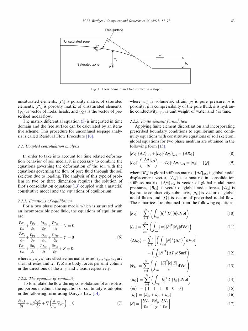
T = {Dpf, Dpf, Dpf, 0, 0, 0}. Dpf is the change in porefluid pressure and it is composed of static hydraulic pres-sure, seepage pressure due to fluid flow in the porous mediaand excess pore pressure due to stress increase in the por-ous media. Pore pressure change a point at A in a slopeas shown in Fig. 1 is

Dpf ¼ Dpseepage þ Dpexcess ð2Þ

where Dpseepage is pore pressure increase due to seepage inthe flow domain and Dpexcess is excess pore pressure dueto stress change.

The excess pore pressures which occur due to stresschange in the domain should be calculated by stress–strainanalysis. These pressures are not steady and they changewith time, i.e. they dissipiate and it is a transient seepageproblem.

2.1. Seepage analysis

The pore pressures due to seepage is determined by seep-age analysis. If the flow domain contains a free surface asshown in Fig. 1 which changes by time, the problembecomes more complicated and it should be analyzed asan unconfined transient seepage problem.

Considering Darcy’s law, the differential equation gov-erning flow through porous saturated incompressiblemedia is

divðk � grad/Þ � Q ¼ So/ot

ð3Þ

where / is the total fluid potential or head = (p/c) + z, p isthe pressure head, z is gravity head, c is fluid density, k ishydraulic conductivity of the medium, Q is appliedsource/sink and S is the specific storage.

And Eq. (3) is assumed to hold in both saturated andunsaturated domains by introducing the definition of k asfollows:

kðpÞ ¼ks in saturated zone

ks � f ðpÞ in unsaturated zone

�ð4Þ

where ks is saturated hydraulic conductivity which is con-stant and f(p) is smooth continuous function of the pres-sure head p.

2.1.1. Finite element formulation

The finite element equations are obtained from the var-iational analysis of Eq. (3) as

½ks�fqg � ½kus�fqg þ ½P us�fqg � ½P us�fqg ¼ fQg ð5Þ

where [ks] is the hydraulic conductivity matrix of satu-rated elements, [kus] is hydraulic conductivity matrix of

w

w

Fig. 1. Flow domain and free surface in a slope.

M.M. Berilgen / Computers and Geotechnics 34 (2007) 81–91 83

unsaturated elements, [Ps] is porosity matrix of saturatedelements, [Ps] is porosity matrix of unsaturated elements,{qs} is vector of nodal heads, and {Q} is the vector of pre-scribed nodal flow.

The matrix differential equation (5) is integrated in timedomain and the free surface can be calculated by an itera-tive scheme. This procedure for unconfined seepage analy-sis is called Residual Flow Procedure [10].

2.2. Coupled consolidation analysis

In order to take into account for time related deforma-tion behavior of soil media, it is necessary to combine theequations governing the deformation of the soil with theequations governing the flow of pore fluid through the soilskeleton due to loading. The analysis of this type of prob-lem in two or three dimension requires the solution ofBiot’s consolidation equations [13] coupled with a materialconstitutive model and the equations of equilibrium.

2.2.1. Equations of equilibriumFor a two phase porous media which is saturated with

an incompressible pore fluid, the equations of equilibriumare

or0xoxþ opf

oxþ osxy

oyþ osxz

ozþ X ¼ 0

or0yoyþ opf

oyþ osxy

oxþ osyz

ozþ Y ¼ 0

or0zozþ opf

ozþ osxz

oxþ osyz

oyþ Z ¼ 0

ð6Þ

where r0x, r0y , r0z are effective normal stresses, sxy, syz, sxz areshear stresses and X, Y, Z are body forces per unit volumein the directions of the x, y and z axis, respectively.

2.2.2. The equation of continuity

To formulate the flow during consolidation of an isotro-pic porous medium, the equation of continuity is adoptedin the following form using Darcy’s Law [14]:

oevol

otþ nb

opf

otþr k

cw

rpf

� �¼ 0 ð7Þ

where evol is volumetric strain, pf is pore pressure, n isporosity, b is compressibility of the pore fluid, k is hydrau-lic conductivity, cw is unit weight of water and t is time.

2.2.3. Finite element formulationApplying finite element discretisation and incorporating

prescribed boundary conditions to equilibrium and conti-nuity equations with constitutive equations of soil skeleton,global equations for two phase medium are obtained in thefollowing form [15]:

½KG�fDdgnG þ ½LG�fDpfgnG ¼ fDRGg ð8Þ

½LG�TfDdgnG

Dt

� �� ½UG�fDpfgnG ¼ ½nG� þ fQg ð9Þ

where [KG] is global stiffness matrix, {Dd}nG is global nodaldisplacement vector, [LG] is submatrix in consolidationstiffness matrix, {Dpf}nG is vector of global nodal porepressures, {RG} is vector of global nodal forces, [UG] ishydraulic conductivity submatrix, [nG] is vector of globalnodal fluxes and {Q} is vector of prescribed nodal flow.These matrices are obtained from the following equations:

½KG� ¼XN

i¼1

ZVol

½B�T½D0�½B�dVol

� �ð10Þ

½LG� ¼XN

i¼1

ZVol

fmg½B�T½N p�dVol

� �ð11Þ

fDRGg ¼XN

i¼1

ZVol

½N �TfDF g� �

dVol

� �

þZ

S½N �TfDTgdSurf

� �ð12Þ

½UG� ¼XN

i¼1

ZVol

½E�T½k�½E�cf

dVol

!ð13Þ

fnGg ¼XN

i¼1

ZVol

½E�T½k�fiGgdVol

� �ð14Þ

fmgT ¼ f 1 1 1 0 0 0 g ð15ÞfiGg ¼ fiGx þ iGy þ iGzg ð16Þ

½E� ¼ oNp

ox;oN p

oy;oN p

oz

� �ð17Þ


where [D 0] is effective constitutive matrix, N and Np areinterpolation functions for displacements and pore pres-sures, respectively, and [B] and [E] contains derivatives ofthe interpolation functions, DF and DT are vector of nodalforces, [k] is hydraulic conductivity matrix and {iG} is theunit vector.

3. Methodology

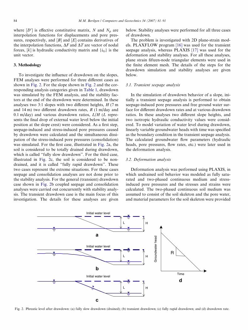
To investigate the influence of drawdown on the slopes,FEM analyses were performed for three different cases asshown in Fig. 2. For the slope shown in Fig. 2 and the cor-responding analysis categories given in Table 1, drawdownwas simulated by the FEM analysis, and the stability fac-tors at the end of the drawdown were determined. In theseanalyses two 3:1 slopes with two different heights, H (7 mand 14 m) two different drawdown rates, R (1 m/day and0.1 m/day) and various drawdown ratios, L/H (L repre-sents the final drop of external water level below the initialposition at the slope crest) were considered. As a first step,seepage-induced and stress-induced pore pressures causedby drawdown were calculated and the simultaneous dissi-pation of the stress-induced pore pressures (consolidation)was simulated. For the first case, illustrated in Fig. 2a, thesoil is considered to be totally drained during drawdown,which is called ‘‘fully slow drawdown’’. For the third case,illustrated in Fig. 2c, the soil is considered to be non-drained, and it is called ‘‘fully rapid drawdown’’. Thesetwo cases represent the extreme situations. For these casesseepage and consolidation analyses are not done prior tothe stability analysis. For the general (transient) drawdowncase shown in Fig. 2b coupled seepage and consolidationanalyses were carried out concurrently with stability analy-sis. The transient drawdown case is the main focus of thisinvestigation. The details for these analyses are given

L

Initial water level

a

b

c

L

Initial water level

L

Initial water level

Fig. 2. Phreatic level after drawdown: (a) fully slow drawdown (drained); (b

below. Stability analyses were performed for all three casesof drawdown.

The problem is investigated with 2D plane-strain mod-els. PLAXFLOW program [16] was used for the transientseepage analysis, whereas PLAXIS [17] was used for thedeformation and stability analyses. For all these analyses,plane strain fifteen-node triangular elements were used inthe finite element mesh. The details of the steps for thedrawdown simulation and stability analyses are givenbelow.

3.1. Transient seepage analysis

In the simulation of drawdown behavior of a slope, ini-tially a transient seepage analysis is performed to obtainseepage-induced pore pressures and free ground water sur-face for different drawdown rates and at various drawdownratios. In these analyses two different slope heights, andtwo isotropic hydraulic conductivity values were consid-ered. To model variation of water level during drawdown,linearly variable groundwater heads with time was specifiedas the boundary condition in the transient seepage analysis.The calculated groundwater flow parameters (hydraulicheads, pore pressures, flow rates, etc.) were later used inthe deformation analysis.

3.2. Deformation analysis

Deformation analysis was performed using PLAXIS, inwhich undrained soil behavior was modeled as fully satu-rated and two-phased continuous medium and stress-induced pore pressures and the stresses and strains werecalculated. The two-phased continuous soil medium wasassumed to consist of the soil skeleton and the pore water,and material parameters for the soil skeleton were provided

H

d

H

H

R

Gro

undw

ater

hea

d

Time

) transient drawdown; (c) fully rapid drawdown; and (d) drawdown rate.

Table 1Analyses types for slope stability during drawdown

Analysis Material behavior Transient seepage Deformation Consolidation Stability

Coupled analysis Undrainedp p p p

Fully slow drawdown Drained NAp

NAp

Fully rapid drawdown Undrained NAp

NAp

NA, not applicable.

a

f

ur

50

Fig. 3. Derivation of stiffness parameters secant modulus Eref50 and

unloading–reloading modulus Erefur from a triaxial test.


in terms of effective stress parameters. To compute thestress-induced pore pressures as realistically as possible,an advanced nonlinear elasto-plastic material model needsto be utilized in the numerical analysis. PLAXIS is capableof utilizing such advanced material models. In this work,‘‘hardening soil model’’ is used for deformation and con-solidation analysis.

3.2.1. Hardening soil model (HSM)

Hardening soil model is an advanced version of theDuncan–Chang model also known as hyperbolic model[18] which captures soil behavior in a very tractable manneron the basis of only two stiffness parameters. The majorinconsistency of this model is that, in contrast to theelasto-plastic type of models, being a purely hypo-elasticmodel it cannot consistently distinguish between loadingand unloading stages. HSM supersedes Duncan–Changmodel, firstly by using the theory of plasticity rather thanthe theory of elasticity, secondly by including soil dilat-ancy, and thirdly by introducing a yield cap. In the model,distinction is made between two types of hardening,namely shear hardening and compression hardening. Shearhardening is used to model irreversible strains due to pri-mary deviatoric loading. Compression hardening is usedfor irreversible plastic strains due to primary compressionin constrained loading and isotropic loading. A cappedMohr–Coulomb type yield surface is allowed to expandduring plastic straining. Total strains are calculated by astress dependent stiffness [19].

Input parameters needed for HSM are the well-knownstrength parameters of internal friction angle /, cohesionintercept c and dialatancy angle w. Soil stiffness is definedby the parameters Eref

50 characterizing the shear behaviorof soil, Eref

oed mainly controlling the volumetric behaviorand Eref

ur the unloading–reloading modulus. An Ohde/Janbu type parameter m controls the stress dependencyof the all three stiffnesses as given by the following equation[20]:

E ¼ Eref c cos u� r0i sin uc cos uþ pref sin u

� �m

ð18Þ

where E shows the stress dependent moduli (E50, Eoed, orEur) corresponding to the related Eref ðEref

50 ;Erefoed; or Eref

ur Þ,m is power for stress level dependency of stiffness, pref is ref-erence stress for stiffness and r 0i is minor principle stress forE50 and Eur, and major principal stress for Eoed. The deri-vation of the above stiffness parameters by a triaxial test isshown in Fig. 3.

3.3. Consolidation analysis

During drawdown, the dissipation, i.e. consolidation, ofthe stress-induced pore pressures will occur in parallel totheir generation. To obtain the dissipated pore pressuresat any stage of drawdown, fully coupled consolidationanalysis was carried out together with the deformationanalysis. The consolidation analysis was performed usingPLAXIS which utilizes Biot’s consolidation theory in 2D[17] and the nonlinear material behavior is taken intoaccount as mentioned before. Although it is possible toconsider the anisotropy in hydraulic conductivity, in thisstudy for the seepage and consolidation analysis the soilmedium was assumed to be isotropic and two typicalhydraulic conductivity values (k = 10�4 and 10�6 cm/s)were used, and all model boundaries except top surfaceswere considered to be impermeable.

3.4. Stability analysis

The stability analysis was performed employingPLAXIS using the stresses calculated as a result of thedeformation and consolidation analyses and utilizing thestrength reduction method. In this method, the factor ofsafety against slope failure is computed through the reduc-tion of the strength parameters at a certain rate ð

PMsfÞ,

as shown in the equation below, and performing the defor-mation analysis.X

Msf ¼tan /input

tan /reduced

¼ cinput

creduced

ð19Þ


In this nonlinear deformation analysis based on the Mohr–Coulomb material model, the maximum

PMsf that pro-

vides the equilibrium is called the factor of safety (FoS).This method is also called the Phi-ci reduction method.The sliding surface does not need to be defined beforehandand is automatically found, therefore, a shear surface clo-ser to the natural sliding surface is defined [8,9].

4. Material parameters

All the material parameters (physical meanings of whichare explained above) used in FEM analyses for the casesshown in Table 1, are given in Table 2.

5. The results of the analysis

To investigate the stability of submerged slopes subjectto drawdown, the groundwater flow and the deformationof the slope following the drawdown was simulated usingthe FEM for two different slope heights (H = 7 m and14 m), two typical soil hydraulic conductivity values(k = 10�4 cm/s and 10�6 cm/s) and two distinct drawdown

Table 2Materials properties for the slope soil considered in the FEM analysis

Material properties Sym

Unit weight of soil cPermeability k

Cohesion intercept c0

Internal friction angle /0

Dilatancy angle WSecant reference stiffness modulus Eref

50

Secant reference oedometer modulus Erefoed

Unloading–reloading reference stiffness modulus Erefur

Poisson ratio n

Reference stress for stiffness pref

Power for stress level dependency m

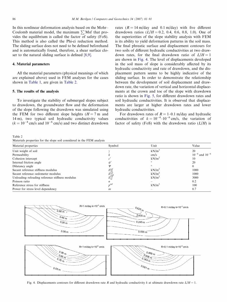
Fig. 4. Displacements contours for different drawdown rate R and

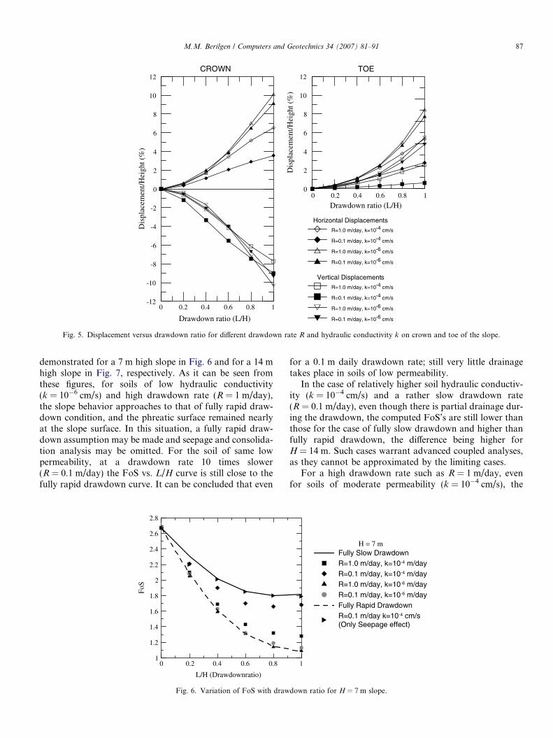
rates (R = 14 m/day and 0.1 m/day) with five differentdrawdown ratios (L/H = 0.2, 0.4, 0.6, 0.8, 1.0). One ofthe superiorities of the slope stability analysis with FEMis its ability to yield deformation patterns in the soil mass.The final phreatic surface and displacement contours fortwo soils of different hydraulic conductivities at two draw-down rates, for the final drawdown ratio of L/H = 1are shown in Fig. 4. The level of displacements developedin the soil mass of slope is considerably affected by itshydraulic conductivity and rate of drawdown, and the dis-placement pattern seems to be highly indicative of thesliding surface. In order to demonstrate the relationshipbetween the development of soil displacement and draw-down rate, the variation of vertical and horizontal displace-ments at the crown and toe of the slope with drawdownratio is shown in Fig. 5, for different drawdown rates andsoil hydraulic conductivities. It is observed that displace-ments are larger at higher drawdown rates and lowerhydraulic conductivities.

For drawdown rates of R = 1–0.1 m/day and hydraulicconductivities of k = 10�4–10�6 cm/s, the variation offactor of safety (FoS) with the drawdown ratio (L/H) is

bol Unit Value

kN/m3 20cm/s 10�4 and 10�6

kN/m2 10� 20� 0kN/m2 1000kN/m2 1000kN/m2 3000– 0.2kN/m2 100– 0.7

hydraulic conductivity k at ultimate drawdown rate L/H = 1.

Drawdown ratio (L/H)

0

2

4

6

8

10

12

Dis

plac

emen

t/Hei

ght (

%)

0 0.2 0.4 0.6 0.8 1

0 0.2 0.4 0.6 0.8 1

Drawdown ratio (L/H)

-12

-10

-8

-6

-4

-2

0

2

4

6

8

10

12

Dis

plac

emen

t/Hei

ght (

%)

Horizontal DisplacementsR=1.0 m/day, k=10-4 cm/s

R=0.1 m/day, k=10-4 cm/s

R=1.0 m/day, k=10-6 cm/s

R=0.1 m/day, k=10-6 cm/s

TOE CROWN

Vertical DisplacementsR=1.0 m/day, k=10-4 cm/s

R=0.1 m/day, k=10-4 cm/s

R=1.0 m/day, k=10-6 cm/s

R=0.1 m/day, k=10-6 cm/s

Fig. 5. Displacement versus drawdown ratio for different drawdown rate R and hydraulic conductivity k on crown and toe of the slope.


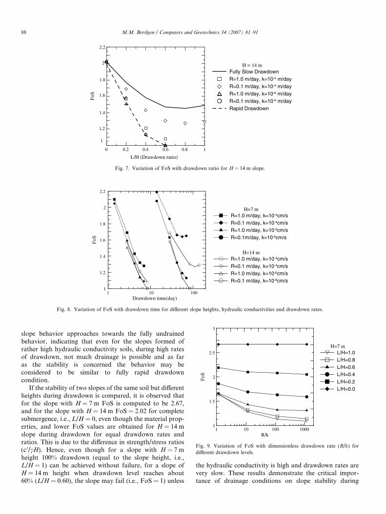
demonstrated for a 7 m high slope in Fig. 6 and for a 14 mhigh slope in Fig. 7, respectively. As it can be seen fromthese figures, for soils of low hydraulic conductivity(k = 10�6 cm/s) and high drawdown rate (R = 1 m/day),the slope behavior approaches to that of fully rapid draw-down condition, and the phreatic surface remained nearlyat the slope surface. In this situation, a fully rapid draw-down assumption may be made and seepage and consolida-tion analysis may be omitted. For the soil of same lowpermeability, at a drawdown rate 10 times slower(R = 0.1 m/day) the FoS vs. L/H curve is still close to thefully rapid drawdown curve. It can be concluded that even

0 0.2 0.4 0.6 0.8

L/H (Drawdownratio)

1

1.2

1.4

1.6

1.8

2

2.2

2.4

2.6

2.8

FoS

Fig. 6. Variation of FoS with draw

for a 0.1 m daily drawdown rate; still very little drainagetakes place in soils of low permeability.

In the case of relatively higher soil hydraulic conductiv-ity (k = 10�4 cm/s) and a rather slow drawdown rate(R = 0.1 m/day), even though there is partial drainage dur-ing the drawdown, the computed FoS’s are still lower thanthose for the case of fully slow drawdown and higher thanfully rapid drawdown, the difference being higher forH = 14 m. Such cases warrant advanced coupled analyses,as they cannot be approximated by the limiting cases.

For a high drawdown rate such as R = 1 m/day, evenfor soils of moderate permeability (k = 10�4 cm/s), the

1

H = 7 mFully Slow DrawdownR=1.0 m/day, k=10-4 m/dayR=0.1 m/day, k=10-4 m/dayR=1.0 m/day, k=10-6 m/dayR=0.1 m/day, k=10-6 m/dayFully Rapid DrawdownR=0.1 m/day k=10-4 cm/s(Only Seepage effect)

down ratio for H = 7 m slope.

0 10.2 0.4 0.6 0.8

L/H (Drawdown ratio)

1

1.2

1.4

1.6

1.8

2

2.2

FoS

H = 14 mFully Slow DrawdownR=1.0 m/day, k=10-4 m/dayR=0.1 m/day, k=10-4 m/dayR=1.0 m/day, k=10-6 m/dayR=0.1 m/day, k=10-6 m/dayRapid Drawdown

Fig. 7. Variation of FoS with drawdown ratio for H = 14 m slope.

1 10 100Drawdown time(day)

1

1.2

1.4

1.6

1.8

2

2.2

FoS

H=7 mR=1.0 m/day, k=10-4cm/sR=0.1 m/day, k=10-4cm/sR=1.0 m/day, k=10-6cm/sR=0.1m/day, k=10-6cm/s

H=14 mR=1.0 m/day, k=10-4cm/sR=0.1 m/day, k=10-4cm/sR=1.0 m/day, k=10-6cm/sR=0.1 m/day, k=10-6cm/s

Fig. 8. Variation of FoS with drawdown time for different slope heights, hydraulic conductivities and drawdown rates.

1 10 100 1000R/k

1

1.5

2

2.5

3

FoS

H=7 mL/H=1.0L/H=0.8L/H=0.6L/H=0.4L/H=0.2L/H=0.0

Fig. 9. Variation of FoS with dimensionless drawdown rate (R/k) fordifferent drawdown levels.


slope behavior approaches towards the fully undrainedbehavior, indicating that even for the slopes formed ofrather high hydraulic conductivity soils, during high ratesof drawdown, not much drainage is possible and as faras the stability is concerned the behavior may beconsidered to be similar to fully rapid drawdowncondition.

If the stability of two slopes of the same soil but differentheights during drawdown is compared, it is observed thatfor the slope with H = 7 m FoS is computed to be 2.67,and for the slope with H = 14 m FoS = 2.02 for completesubmergence, i.e., L/H = 0, even though the material prop-erties, and lower FoS values are obtained for H = 14 mslope during drawdown for equal drawdown rates andratios. This is due to the difference in strength/stress ratios(c 0/cH). Hence, even though for a slope with H = 7 mheight 100% drawdown (equal to the slope height, i.e.,L/H = 1) can be achieved without failure, for a slope ofH = 14 m height when drawdown level reaches about60% (L/H = 0.60), the slope may fail (i.e., FoS = 1) unless

the hydraulic conductivity is high and drawdown rates arevery slow. These results demonstrate the critical impor-tance of drainage conditions on slope stability during


drawdown, especially for slopes which do not possess ahigh degree of safety prior to drawdown.

The variation of the FoS as drawdown progresses isdemonstrated in Figs. 8 and 9 as deduced from the resultsof the analysis for different slope heights, drawdown ratesand hydraulic conductivities. Fig. 8 shows the variation

0.01 0.1 1 10 100T

0.75

1

1.25

1.5

1.75

2

2.25

FoS

Fig. 10. Variation of FoS

0 0.2 0.4 0.6 0.8 1u0-u u0

0

5

10

15

20

25

Ele

vatio

n (m

)

R=1 m/day, k=10-4 cm/s

0 0.2 0.4 0.6 0.8 1u0-u u0

0

5

10

15

20

25

Ele

vatio

n (m

)

R=1 m/day, k=10-6 cm/s

Fig. 11. Variation of normalized excess pore

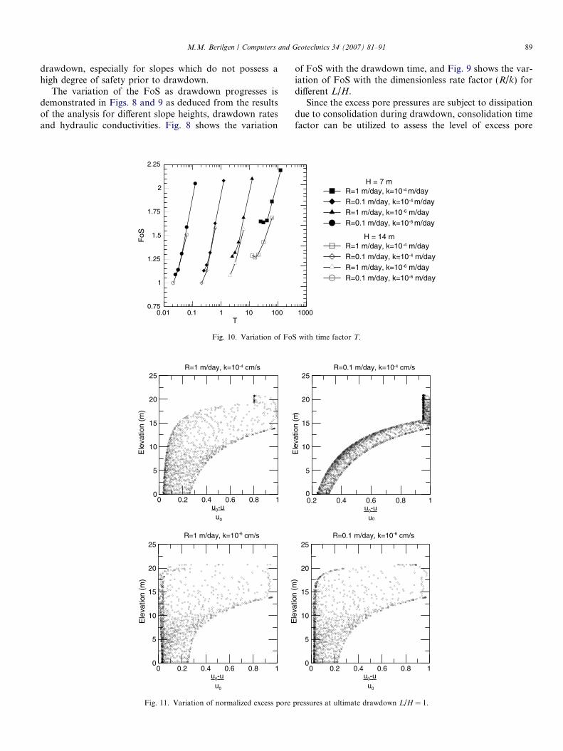
of FoS with the drawdown time, and Fig. 9 shows the var-iation of FoS with the dimensionless rate factor (R/k) fordifferent L/H.

Since the excess pore pressures are subject to dissipationdue to consolidation during drawdown, consolidation timefactor can be utilized to assess the level of excess pore

1000

H = 7 mR=1 m/day, k=10-4 m/dayR=0.1 m/day, k=10-4 m/dayR=1 m/day, k=10-6 m/dayR=0.1 m/day, k=10-6 m/day

H = 14 mR=1 m/day, k=10-4 m/dayR=0.1 m/day, k=10-4 m/dayR=1 m/day, k=10-6 m/dayR=0.1 m/day, k=10-6 m/day

with time factor T.

0.2 0.4 0.6 0.8 1u0-u u0

0

5

10

15

20

25

Ele

vatio

n (m

)

R=0.1 m/day, k=10-4 cm/s

0 0.2 0.4 0.6 0.8 1u0-u u0

0

5

10

15

20

25

Ele

vatio

n (m

)

R=0.1 m/day, k=10-6 cm/s

pressures at ultimate drawdown L/H = 1.


pressures and their effect of slope stability [7]. In 1D con-solidation, the time factor T for any drawdown time td

(i.e., the time it takes to reach L depending on R), can beobtained from

T ¼ cvtd

H 2ð20Þ

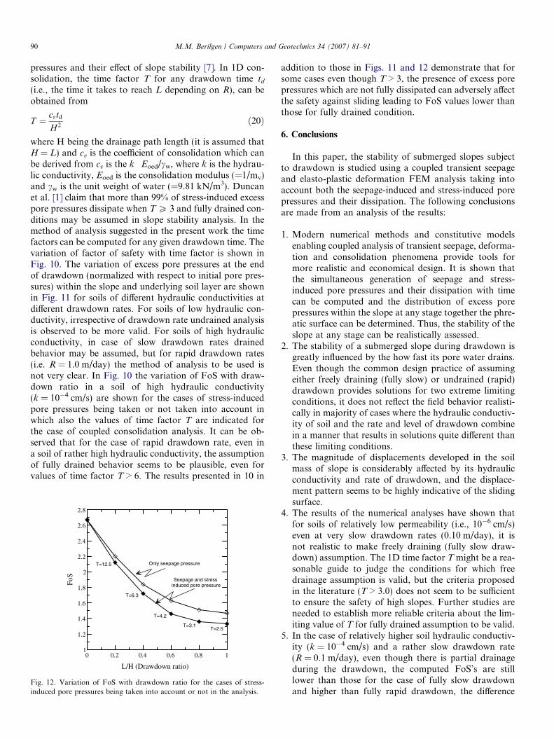
where H being the drainage path length (it is assumed thatH = L) and cv is the coefficient of consolidation which canbe derived from cv is the k Æ Eoed/cw, where k is the hydrau-lic conductivity, Eoed is the consolidation modulus (=1/mv)and cw is the unit weight of water (=9.81 kN/m3). Duncanet al. [1] claim that more than 99% of stress-induced excesspore pressures dissipate when T P 3 and fully drained con-ditions may be assumed in slope stability analysis. In themethod of analysis suggested in the present work the timefactors can be computed for any given drawdown time. Thevariation of factor of safety with time factor is shown inFig. 10. The variation of excess pore pressures at the endof drawdown (normalized with respect to initial pore pres-sures) within the slope and underlying soil layer are shownin Fig. 11 for soils of different hydraulic conductivities atdifferent drawdown rates. For soils of low hydraulic con-ductivity, irrespective of drawdown rate undrained analysisis observed to be more valid. For soils of high hydraulicconductivity, in case of slow drawdown rates drainedbehavior may be assumed, but for rapid drawdown rates(i.e. R = 1.0 m/day) the method of analysis to be used isnot very clear. In Fig. 10 the variation of FoS with draw-down ratio in a soil of high hydraulic conductivity(k = 10�4 cm/s) are shown for the cases of stress-inducedpore pressures being taken or not taken into account inwhich also the values of time factor T are indicated forthe case of coupled consolidation analysis. It can be ob-served that for the case of rapid drawdown rate, even ina soil of rather high hydraulic conductivity, the assumptionof fully drained behavior seems to be plausible, even forvalues of time factor T > 6. The results presented in 10 in

0 0.2 0.4 0.6 0.8 1

L/H (Drawdown ratio)

1

1.2

1.4

1.6

1.8

2

2.2

2.4

2.6

2.8

FoS

T=12.5

T=6.3

T=4.2

T=3.1T=2.5

Only seepage pressure

Seepage and stress induced pore pressure

Fig. 12. Variation of FoS with drawdown ratio for the cases of stress-induced pore pressures being taken into account or not in the analysis.

addition to those in Figs. 11 and 12 demonstrate that forsome cases even though T > 3, the presence of excess porepressures which are not fully dissipated can adversely affectthe safety against sliding leading to FoS values lower thanthose for fully drained condition.

6. Conclusions

In this paper, the stability of submerged slopes subjectto drawdown is studied using a coupled transient seepageand elasto-plastic deformation FEM analysis taking intoaccount both the seepage-induced and stress-induced porepressures and their dissipation. The following conclusionsare made from an analysis of the results:

1. Modern numerical methods and constitutive modelsenabling coupled analysis of transient seepage, deforma-tion and consolidation phenomena provide tools formore realistic and economical design. It is shown thatthe simultaneous generation of seepage and stress-induced pore pressures and their dissipation with timecan be computed and the distribution of excess porepressures within the slope at any stage together the phre-atic surface can be determined. Thus, the stability of theslope at any stage can be realistically assessed.

2. The stability of a submerged slope during drawdown isgreatly influenced by the how fast its pore water drains.Even though the common design practice of assumingeither freely draining (fully slow) or undrained (rapid)drawdown provides solutions for two extreme limitingconditions, it does not reflect the field behavior realisti-cally in majority of cases where the hydraulic conductiv-ity of soil and the rate and level of drawdown combinein a manner that results in solutions quite different thanthese limiting conditions.

3. The magnitude of displacements developed in the soilmass of slope is considerably affected by its hydraulicconductivity and rate of drawdown, and the displace-ment pattern seems to be highly indicative of the slidingsurface.

4. The results of the numerical analyses have shown thatfor soils of relatively low permeability (i.e., 10�6 cm/s)even at very slow drawdown rates (0.10 m/day), it isnot realistic to make freely draining (fully slow draw-down) assumption. The 1D time factor T might be a rea-sonable guide to judge the conditions for which freedrainage assumption is valid, but the criteria proposedin the literature (T > 3.0) does not seem to be sufficientto ensure the safety of high slopes. Further studies areneeded to establish more reliable criteria about the lim-iting value of T for fully drained assumption to be valid.

5. In the case of relatively higher soil hydraulic conductiv-ity (k = 10�4 cm/s) and a rather slow drawdown rate(R = 0.1 m/day), even though there is partial drainageduring the drawdown, the computed FoS’s are stilllower than those for the case of fully slow drawdownand higher than fully rapid drawdown, the difference


being higher for H = 14 m. Such cases warrantadvanced coupled analyses, as they cannot be approxi-mated by the limiting cases.

6. The results indicate that it is important to take stress-induced pore pressures and their dissipation intoaccount in addition to seepage-induced pore pressuresin fine-grained soils.

Acknowledgements

The writer acknowledge for the important suggestionand extensive review on the paper made by Professors Tun-cer B. Edil from University of Wisconsin, Madison, and I.Kutay Ozaydin from Yildiz Technical University, Istanbul.

References

[1] Duncan JM, Wrigth SG, Wong KS. Slope stability during rapiddrawdown. In: Proceedings of the H. Bolton seed memorial sympo-sium, Vol. 2; May 1990. p. 253–72.

[2] US Army Corps Of Engineers. Engineering and design manual –slope stability, Engineer Manual EM 1110-2-1902, Department of theArmy, Corps of Engineers, Washington (DC); 2003.

[3] Lowe J, Karafiath L. Stability of earth dams upon drawdown. In:Proceedings of the first Panamerican conference on soil mechanicsand foundation engineering, Mexico City, vol. 2; 1960. p. 537–52.

[4] Svano G, Nordal S. Undrained effective stability analysis. In:Proceedings of the ninth European conference on soil mechanicsand foundation, Dublin; 1987.

[5] Wright SG, Duncan JM. An examination of slope stability compu-tation procedures for sudden drawdown, US Army Corps Engineer-ing. Waterway Experiment Station, Vicksburg (MS); 1987.

[6] Desai CS. Drawdown analysis of slopes by numerical methods. JGeotech Eng, Proc ASCE 1977;109(7):946–60.

[7] Duncan JM, Wright SG. Soil strength and slope stability. Hoboken(NJ): John Wiley & Sons; 2005.

[8] Dawson EM, Roth WH, Drescher A. Slope stability analysis bystrength reduction. Geotechnique 1999;49(6):835–40.

[9] Griffiths DV, Lane PA. Slope stability analysis by finite elements.Geotechnique 1999;49(3):387–403.

[10] Lane PA, Griffiths DV. Assessment of stability of slopes underdrawdown conditions. J Geotech Geoenviron Eng 2000;126(5):443–50.

[11] Li GC, Desai CS. Stress and seepage analysis of earth dams. J GE,Proc ASCE 1983;103(GT7):667–76.

[12] Borja RI, Kishnani SS. Movement of slopes during rapid and slowdrawdown. In: Raymond B. Seed, editor. Stability and performance ofslopes and embankments II. In: Proceedings of a special conference bnthe Geotechnical Engineering Division of ASCE, Berkeley (CA); 1992.

[13] Biot MA. General theory of three-dimensional consolidation. J ApplPhys 1941;12:155–64.

[14] Verrujit A. Computational geomechanics. Kluwer Academic Pub-lisher; 1995.

[15] Potts DM, Zdravkovic L. Finite element analysis in geotechnicalengineering-theory. Thomas Telford Publishing; 1999.

[16] Brinkgreve RBJ, Al-Khoury R, van Esch JM. Plaxflow user manualVersion 1. Balkema; 2003.

[17] Brinkgreve RBJ. Plaxis finite element code for soil and rock analyses,Version 8. Balkema; 2001.

[18] Duncan JM, Chang CY. Nonlinear analysis of stress–strain in soils. JSoil Mech Found Eng Div, ASCE 1970;96(SM5):1629–53.

[19] Schnaz T, Vermeer PA, Bonnier PG. Formulation and verification ofthe hardening-soil model. In: Brinkgreve RBJ, editor. Beyond 2000 inComputational Geotechnics. Balkema; 1999.

[20] Vermeer PA, Benz T, Schwab R. On the practical use of advancedconstitutive laws for finite element foundation simulations. In:Magnan, J.-P., Droniuc N, editors. FONDSUP 2003: Symposiuminternational sur les fondations superficielles, Presses de l’ENPC/LCPC, Paris, vol. 1; 2003. p. 49–56.

Documents

Investigation of stability of slopes under drawdown conditions