Investigation of Piezoelectric Flaps for Load …etd.dtu.dk/thesis/259219/ris_r_1702.pdfInvestigation of Piezoelectric Flaps for Load Alleviation Using CFD Joachim Christian Heinz

Author: Joachim Christian Heinz Title: Investigation of Piezoelectric Flaps for Load Alleviation Using CFD Division: Wind Energy Division

Risø-R-1702(EN) 2009 Published on www.risoe.dtu.dk in March 2010

Abstract (max. 2000 char.): Cost efficient wind power generation demands for large wind turbines with a long lifetime. These demands place high interests on sophisticated load control techniques such as deformable trailing edge flaps. In this work a previously tested prototype airfoil was investigated by using the 2D incompressible RANS solver EllipSys2D. The prototype was built with a Risø-B1-18 airfoil where piezoelectric actuators THUNDER TH-6R were attached at the trailing edge to realize a movable flap. The results of the simulation were compared to measurements of the previous wind tunnel test and comprehensive steady state computations were conducted to gain information about the general airfoil properties. The model was subsequently used to investigate aero-servo-elastic effects on the 2D airfoil section exposed to a fluctuating inflow. It is explained how a fluctuating inflow was simulated with EllipSys2D and how the CFD solver was coupled with a 3 DOF structural model and with two different control algorithms. Control 1 used the measured AOA in front of the LE as input, Control 2 used the pressure difference between suction and pressure side as input. The model showed a substantial load reduction potential for the present prototype airfoil. For a wind step from 10 m/s to 10.5 m/s the standard deviation of the structural deflection normal to the rotor plane could be reduced with up to 98 % (Control 1) and 96 % (Control 2). A 4 s turbulent inflow with TI=2.2 % could be reduced with up to 81 % (Control 1) and 82 % (Control 2). For a 12 s inflow with TI=2.4 % the standard deviation could be reduced with up to 68 % (Control 1) and 67 % (Control 2). The influence of possible time lags inside the control loop on the reduction potential of the prototype was also investigated. For a 12 s inflow with a tripled turbulence intensity of TI=7.7 % the prototype airfoil could still reach a reduction of up to 54 %. For an extended flap range of -6 to +6 degrees the reduction could be returned to 66 %.

ISSN 0106-2840 ISBN 978-87-550-3767-0

Contract no.:

Group's own reg. no.: (Føniks PSP-element)

Sponsorship:

Cover :

Pages: 75 Tables: References:

Information Service Department Risø National Laboratory for Sustainable Energy Technical University of Denmark P.O.Box 49 DK-4000 Roskilde Denmark Telephone +45 46774005 [email protected] Fax +45 46774013 www.risoe.dtu.dk

Investigation ofPiezoelectric Flaps for LoadAlleviation Using CFDJoachim Christian HeinzM.Sc. Thesis

Risø National Laboratory, Roskilde, Denmark2009

Contents

Nomenclature 7

1 Introduction 9

2 EllipSys2D 102.1 Moving the Grid / Inlet Velocity 11

2.1.1 Comment on the force output: 112.1.2 Comment on the translatoric motion: 11

2.2 Morphing the grid 11

3 Generation of Airfoil Shape 123.1 Method 133.2 Definition of the Flap Deflection Angle β 153.3 Maximum Deflection Angles of the Prototype 15

4 Grid Study 174.1 Steady State Computations 174.2 Unsteady Computations 19

5 Simulations and Measurements 215.1 Fixed AOA / Fixed flap angle 215.2 Harmonic motion of AOA / Fixed flap angle 255.3 Fixed AOA / Harmonic motion of flap angle 285.4 Harmonic motion of AOA / Harmonic motion of flap angle 33

6 Further Properties of the Airfoil 34

7 Aeroelastic Model 417.1 Structural Model 417.2 Aerodynamic Model 42

7.2.1 Flow situation in front of the airfoil 427.2.2 Describing the Flow Situation in EllipSys2D 44

7.3 Flowchart of the aeroelastic model 477.4 Validation of the Model 48

8 Aero-Servo-Elastic Model 508.1 Control 1 518.2 Control 2 528.3 Reference Time Window 538.4 Maximum Actuation Velocity, Maximum Flap Angles, Time Delay548.5 Flowchart of the Aero-Servo-Elastic Model 55

9 Results of Test Cases 569.1 Definition of Std(y) and reduction potential RStd(y) 569.2 Airfoil exposed to wind step 579.3 Airfoil exposed to 4 s turbulent wind with TI = 2.2 % 609.4 Airfoil exposed to 12 s turbulent wind field with TI = 2.4 % 649.5 Airfoil exposed to 12 s turbulent wind field with TI = 7.7 % 64

4

9.6 Comment on the results 65

10 Conclusion and Future Work 6710.1 Conclusion 6710.2 Future Work 69

References 70

Appendix 71

A Non-dimensionalized calculation in EllipSys2D 71

B Omitting transient forces during a fluctuating inflow 71

C Input file and Computational Time 72

5

Nomenclature

Roman symbols

cx,cx,cθ Damping coefficients of the structural model [Ns/m]c Total chord length of the airfoil (including attached flap) [m]d1 Distance from pitot tube measurement to LE [m]d2 Distance from LE to pressure taps [m]dCl/dβ efficiency of the flap [1/rad]k Reduced frequency (k = ωc/(2U)) [-]kx,kx,kθ spring stiffnesses of the structural model [N/m]l Distance from LE to CG [m]m Mass of airfoil section [kg]uinlet x-component of inlet velocity in EllipSys2D

(CFD coordinates) [-]vinlet y-component of inlet velocity in EllipSys2D

(CFD coordinates) [-]r Radial blade position of investigated airfoil section [m]rx Translatoric motion in x of moving mesh in EllipSys2D

(CFD coordinates) [-]ry Translatoric motion in y of moving mesh in EllipSys2D

(CFD coordinates) [-]t Time (used in structural model) [s]t∗ Non-dim. time (used in aerodynamic model) [-]tdelay Time delay inside the control [s]xstruct Structural deflection in x (structural coordinates) [m]x∗struct Non-dim. structural deflection in x

(structural coordinates) [-]ystruct Structural deflection in y (structural coordinates) [m]y∗struct Non-dim. structural deflection in y

(structural coordinates) [-]Aα Gain parameter of Control 1 [-]Aα Gain parameter of Control 2 [r/Pa]Cn Normal force coeff. (in x of structural coordinates) [-]Ct Tangential force coeff. (in y of structural coordinates) [-]Fx Tangential force in x (structural coordinates) [N]Fy Normal force in y (structural coordinates) [N]Fθ Moment around RC [Nm]F ∗x,CFD Non-dim. force in x (CFD coordinates) [-]F ∗y,CFD Non-dim. force in y (CFD coordinates) [-]F ∗θ,CFD Non-dim. moment around RC [-]ICG Moment of inertia around CG [kg m2]U∞ Free-stream velocity [m/s]U∗∞ Non-dim. free-stream velocity [-]Va Axial wind velocity [m/s]V ∗a Non-dim. axial wind velocity [-]Vrot Rotational velocity of blade at r [m]V ∗rot Non-dim. rotational velocity of blade at r [-]

7

Greek symbols

α Angle of attack after structural motion is addedαm Mean angle of attack during pitching motionαpresc Angle of attack before structural motion is addedβ Flap deflection angleβmax Maximum deflection angle of the THUNDER TH-6R actuatorβmin Minimum deflection angle of the THUNDER TH-6R actuatorη Normal direction of grid coordinatesζ Rotational angle between coordinate system 4 and 5θgeom Pitch angle of the bladeθstruct Structural deflection around RCκ Phase shift between prescribed pitching and flapping motionϕ Rotational angle of moving mesh in EllipSys2D (rotation around RC)ξ Tangential direction of grid coordinatesφ Flow angle after structural motion is addedφpresc Flow angle before structural motion is addedξ Rotational angle between coordinate system 4 and 5

Abbreviations

2 D 2-DimensionalAOA Angle of attackCFD Computational Fluid DynamicsCG Center of gravity of airfoil sectionDOF Degree of freedomDTEG Deformable trailing edge geometryLE Leading edgeRC Rotational center of airfoil section and of moving mesh

8

1 IntroductionDuring normal operation, wind turbine blades are constantly subjected to fluctuating in-flow conditions. This is due to the unsteady nature of the wind, the influence of the tower,wind shear effects and operation in a yawed position. The fluctuations in the inflow causeconstantly changing loads on the blades which can in turn cause fatigue damage. Reduc-ing the fatigue loads on the blades can lead to lighter blades and reduce the loads on othercomponents such as bearings, drive train and tower. As a consequence the lifetime and thesize of the wind turbines can be increased which makes wind energy potentially cheaperand even more competitive to other energy sources.

Recent work has shown that for Mega-Watt size wind turbines individual pitching canalleviate load increments from yaw-errors, wind shear, gusts, and turbulence consider-ably [1]. Compared to a collective pitch, where all blades are pitched equally, it is shownthat with individual pitching the fatigue loads at the hub can be reduced with 28%. How-ever, pitching a blade means that large masses have to be moved and the actuation speedis limited. Especially the pitching mechanisms of large turbines are thus limited in itsability to react on quick changes in the incoming wind field.

In recent years research put a focus on more sophisticated load control techniques. Agood overview of the presently investigated concepts is given in [2]. It is reported that theconcept of a deformable trailing edge geometry (DTEG) represents an effective and suit-able technique to alleviate the fluctuating loads on large wind turbines. A change of thetrailing edge geometry by using a small flap or a tab can be accomplished much quickerthan turning a whole blade during pitching and this increases the ability to react on quickchanges of the encountered wind field. Additionally, DTEG devices can be actuated indi-vidually over the radial blade position and they can thus much better accommodate to therespective wind situations seen by the blade.One concept to change the aerodynamic forces of a wind turbine blade with a DTEGis by using a Gurney flap like device, also called a microtab. Wind tunnel tests by YenNakafuji et al. [3] and CFD computations by Chow and van Dam [4] demonstrate a sig-nificant potential for load alleviation. Van Dam found that microtabs could increase thelift coefficient Cl in the linear range of the lift curve by 50% while the increase in dragwas modest.Previous work at Risø National Laboratory, Denmark, showed a high potential of loadalleviation by using a deformable flap at the trailing edge. With a 2 D aero-servo-elasticmodel Buhl et al. [5] showed that the standard deviation of the normal force on a 2 Dairfoil section, suspended with springs and dampers, could be reduced with up to 95% ifthe airfoil experiences a sudden wind step from 10 m/s to 12 m/s. When the airfoil wasexposed to a turbulent wind field with 10% turbulence intensity the normal force could bereduced with up to 81%. Andersen [6] found in a 3 D aero-servo-elastic model of a VestasV66 turbine, that for a wind field with 10% turbulence intensity the equivalent flapwiseblade root moment can be reduced with 60%. In these computations effects like time lag,signal noise and maximum power consumption of the flap were included. The models in[5] and [6] both calculate the aerodynamic loads with a very time efficient unsteady po-tential flow solver developed by Gaunaa [7]. The solver uses thin airfoil theory where theairfoil is represented only by its camberline which can deflect in the trailing edge regionin order to simulate the flapping motion.

As the theory showed huge potentials of load alleviation, it was decided to build a pro-totype airfoil and test its properties in a wind tunnel. A Risø-B1-18 airfoil was equippedwith piezoelectric THUNDER TH-6R actuators in order to realize the deformable trail-ing edge. Piezoelectric elements deform gradually and thus maintain a smooth transition

9

between airfoil and flap which then corresponds to the suggested flap shape of Trold-borg [8]. Tests with the airfoil for a step change in the flap angle from β = −3 ◦ toβ = 1.8 ◦ showed that the obtainable ∆Cl lied between 0.1 and 0.13 in the linear partof the lift curve. Counteracting a sinusoidal pitching motion of f = 1.63Hz and a vary-ing AOA of −3.6 ◦ ≤ α ≤= 5.4 ◦ with a phase shifted sinusoidal flapping motion of−3 ◦ ≤ β ≤ 1.8 ◦ reduced the lift amplitude with approximately 80%.

These results place a high interest on using piezoelectric actuators as deformable trailingedge flaps. Therefore, the Risø-B1-18 airfoil equipped with THUNDER TH-6R actuatorsis investigated closer in this work.A detailed model of the prototype airfoil shape is used as input for CFD calculationsusing the 2 D incompressible Reynolds averaged solver EllipSys2D. The possibility ofEllipSys2D to simulate a prescribed pitching and flapping motion was used to comparethe wind tunnel measurements with CFD calculations. These comparisons (see Chap-ter 5) give a better understanding of the prototype airfoil properties and the wind tunnelmeasurements. In Chapter 6 crucial steady state properties of the airfoil were calculated,which can then be used inside other simulation models, such as the dynamic stall modelof Andersen [9].Afterwards, a 3 DOF structural model and two suitable control algorithm are coupledwith EllipSys2D. In Chapter 7 it is explained how existing routines of EllipSys2D areused in order to connect the structural model with the solver and how the simulation of afluctuating inflow is realized. In Chapter 8 two different control strategies are presentedand their respective control algorithms are implemented. Thus it is possible to investigatethe aero-servo-elastic behaviour of the prototype airfoil (or of any other airfoil) using aNavier-Stokes flow solver, which takes viscous effects inside the flow field into account.The new aero-servo-elastic model is finally used in Chapter 9 to investigate the load re-duction potential of the prototype airfoil exposed to a wind step and a fluctuating inflow.

2 EllipSys2DThe CFD flow solver used in this work is EllipSys2D developed by Michelsen [10],[11] and Sørensen [12]. This code solves the incompressible Reynolds averaged Navier-Stokes equations (RANS) using primitive variables (u, v and p) in curvilinear coordinatesthrough a multiblock finite volume discretization approach. For incompressible flow anadditional equation is needed for the pressure, and the standard practice is to derive apressure equation (Poisson equation) by combining the continuity equation with the mo-mentum equation. The momentum and pressure equations are then used in a predictor-corrector fashion (PISO algorithm) to determine the pressure and velocities of the newtime step. The third order accurate QUICK scheme is used to project the convective ve-locities to the cell faces. Information about the PISO algorithm and the QUICK schemecan be found in [13].The overall EllipSys2D computations are proven to be second orderaccurate both in time and in space.The k − ω SST (Shear Stress Transport) turbulence model by Menter [14] was used inthis work. The model has been proven to give very promissing results for 2D airfoil flows[15]. The model is constructed as a blend of the original k − ω model by Wilcox in thenear wall region and the k − ε model in the outer region. The two latter models are de-scribed in e.g. [13].The simulations in this work are carried out under the assumption of a fully turbulentflow. Fully turbulent simulations are considered to provide reasonable results, especiallyif comparisons with measurements of wind tunnels with fairly high turbulence levels arecarried out.The grid generation is accomplished with HypGrid2D developed by Sørensen [16]. The

10

grid generator is using a hyperbolic mesh generation procedure, based on an equation oforthogonality and an equation for the cell face area. The generated grid can be seperatedin several blocks of prescribed size in order to allow parallel (multiblock) computations.

2.1 Moving the Grid / Inlet VelocityIn order to simulate a motion of the airfoil, EllipSys2D provides a routine to move thegrid. This routine accounts for the additional fluxes, which arise when the cell vertices aremoved. As indicated in Figure 1, the translatoric motions rx and ry as well as a rotationϕ are feasible.In Chapter 5 the variable ϕ is used to describe a prescribed harmonic pitching motionof the airfoil in order to compare the results of wind tunnel measurements with CFDcomputations. In Chapter 7, where the CFD solver is coupled with a 3 DOF structuralmodel, the variables rx, ry and ϕ will be used to describe arbitrary structural motions ofthe airfoil.Besides changing the rotational angle ϕ of the moving mesh, the angle between airfoiland inflow can also be adjusted with the two inlet velocities uinlet and vinlet at the domainboundaries. How the several variables are finally used to describe a fluctuating inflow isexplained in Section 7.2.2.

2.1.1 Comment on the force output:

It is important to note, that the calculated aerodynamic forces Fx,CFD ∗ and Fy,CFD ∗

are always given in the direction of the fixed CFD coordinate system. A rotation in ϕ doesnot change the direction of the forces.

2.1.2 Comment on the translatoric motion:

At each time step the translatoric positions of the moving mesh can be defined by thevariables rx and ry while the respective translatoric velocities can not be given directlyas input. Instead EllipSys derives the translatoric velocities and thus the additional fluxesthrough the cell vertices from the given positions by a first order difference approxima-tion.

2.2 Morphing the gridTo accomplish the flap motion, two meshed airfoils are used as input - one with the max-imum and one with the minimum flap angle. As indicated in Figure 2 the actual grid isthen generated by a linear interpolation between the grid points of these two meshes. Gridpoints which are located far away from the movable flap have the same positions for bothflap positions and thus do not feel the morphing procedure.With this morphing technique the respective grid points move on a straight line from themaximum to the minimum flap configuration. This does not exactly correspond to thereal motion, where the points move on an arc around the flap hinge point. However, forsmall changes in the flap angle β the introduced error is negligible. In this work onlysmall changes in β are investigated and the linear interpolation technique is considered tobe adequate.In previous work such as [8] the flap was only moved with a prescribed harmonic motion.In Chapter 8 this will be changed and an implemented control algorithm will control theflap motion.

11

Figure 1. Translatoric motion and rotation of the movable mesh / Definition of inlet ve-locity at the domain boundary

Figure 2. Linear interpolation between the 2 airfoils

3 Generation of Airfoil ShapeIn this work the behaviour of the Risø B1-18 airfoil equipped with a THUNDER TH-6Rpiezoelectric actuator will be investigated. The baseline airfoil of the prototype, whichwas used in the VELUX wind tunnel tests, has a chord length of 0.6 m. At the rear part ofits pressure side, the piezoelectric actuators (see Figure 3) were attached with an overlapof about 1 cm. Before the flaps were attached, some material had been milled away fromthe pressure side of the airfoil in order to ensure a smooth transition between the two

12

components. The resulting airfoil had a total chord length of about c = 0.66 m. A pictureof the prototype is shown in Figure 4.

Figure 3. The Thunder TH-6R actuator from Face International Cooperation

Figure 4. Picture of prototype

3.1 MethodThe 2 D airfoil geometry is generated with Matlab. The intention is to generate a quitedetailed airfoil geometry in order to conduct simulations very close to the real case. Thecoordinates for the prototype airfoil can not be obtained by simply measuring the airfoil,as no sufficiently exact measuring methods have been available. Therefore it is decidedto use the exactly known geometries of the single components and put them virtually to-gether. To attach the flap at the correct position and with the correct angle to the airfoil,

13

several coordinate systems are defined on the baseline airfoil (see Figure 5). In the fol-lowing the position and orientation of the coordinate systems are listed. As the airfoil hasa blunt trailing edge, it is necessary to distinguish between the "‘central TE point"’, whichis defined as the intersection between camber line and airfoil contour, and the "lower TEpoint", which is located at the lower edge of the blunt trailing edge.

- System 1: origin at LE, x-axis tangential to chord line- System 2: origin at central TE point, x-axis tangential to chord line- System 3: origin at lower TE point, x-axis tangential to chord line- System 4: origin at lower TE point, x-axis tangential to pressure side

Figure 5. Coordinate Systems on the baseline airfoil

The geometry of the piezoelectric actuator is described in a separate coordinate system,i.e. coordinate system 5 (see Figure 6). The origin of coordinate system 5 is moved 1 cminside of the actuator. This is due to the overlap between airfoil and actuator. Attachingthe actuator to the baseline airfoil means that the origin of coordinate system 5 and theorigin of coordinate system 4 coincide. To ensure a smooth transition between actuatorand baseline airfoil, the x-axis of system 4 (which is tangentially aligned with the pressureside of the airfoil) has to be tangentially aligned with the actuator surface. This results ina certain rotation angle ζ between coordinate system 4 and 5.

Assuming that the camberline of the flap has the shape of a circular arc, two measuresare enough to determine its geometry. It is the footprint size and the dome height shownin Figure 6. The deformation shape of the piezoelectric actuator depends on the appliedvoltage. To determine the deformation shape for a certain voltage, the respective foot-print size and dome height of the actuator are derived out of the THUNDER TH-6R datasheet. Given the geometry of the flap camberline, simple geometrical formulas are usedto calculate the rotation ζ between coordinate system 4 and 5 which ensures a smoothtransition between actuator and baseline airfoil.

14

Finally the predefined flap contour is built around the flap camberline which is then at-tached to the contour of the baseline airfoil.

Figure 6. Coordinate System on the Piezoelectric Actuator

3.2 Definition of the Flap Deflection Angle βThroughout this work, the flap deflection is described with the flap deflection angle β. Itis thus important to note how this angle is defined. The reference line is the line betweenthe flap root point and the very tip of the flap at an applied voltage of 0 V. In Figure 7this reference line corresponds to the x-axis of coordinate system 5 for a rotation angle ofζ 0V , where ζ 0V is the angle for an applied voltage of 0 V. According to previous work theflap angle is defined positive for a clockwise rotation. Flapping downwards correspondsto an increase in β, flapping upwards corresponds to a decrease in β. In terms of the aboveintroduced rotation angle ζ the flapping angle β can be calculated with

β = ζ − ζ 0V (1)

It should be mentioned here that applying a positive voltage to the piezoelectric actuatorwill bend the flap upwards towards negative flapping angles. Applying a negative voltagewill bend the actuator downwards towards positive flapping angles.

3.3 Maximum Deflection Angles of the PrototypeThe generated airfoil for 0 V is shown in Figure 8. Figure 9 shows the rear part of theairfoil in a bigger scale. Additionally the deflection shapes for +750 V and -450 V are il-lustrated. These are the maximum voltages which could be applied to the tested prototypeand thus, the respective deflection shapes represent the maximum flap angles βmin andβmax.With equation (1) the maximum flap deflection angles of the generated airfoil can be cal-culated. The calculated angles βmin = −5.3 ◦ and βmax = 2.2 ◦ correspond exactly tothe maximum deflection angles measured on the real prototype, when a voltage of +750 Vand -450 V was applied. Thus, the above explained method of the airfoil generation results

15

in the correct flap angles β. As β is generated via ζ and thus via the voltage-dependentfootprint and dome height of the piezoelectric actuator, it can also be concluded that thewhole shape of the flap is captured accurately.

Figure 7. Definition of the flap deflection angle β

Figure 8. Airfoil with attached flap

16

Figure 9. Maximum deflection shapes of the flap

4 Grid Study

4.1 Steady State ComputationsThe grid around the airfoil is generated with HypGrid2D [16]. Although the tip of thetrailing edge flap is quite sharp an O-mesh was generated around the geometry. Closeto the leading edge and close to other areas where high pressure gradients are expected,the cell size in tangential direction (ξ) is reduced in order to increase the accuracy of thecomputations. Especially at the thin trailing edge flap, the cell size has to be chosen quitesmall in order to catch the detailed geometry of the piezoelectric flap.Before starting with thorough computations, it is crucial to check if the generated grid iscapable of resolving the flow sufficiently and thus a grid independence study is carriedout. In the work of Troldborg [8] some indication were given about how the grid should begenerated. The domain height was set to hTot = 20 · c and the height of the cells situatedclosest to the airfoil surface was set to hη=1,2 = 10−6 · c. This corresponds to a maxi-mum y+ value of around 0.2 which is considered to be sufficient to resolve the boundarylayer properly. Troldborg thus used a grid of 256 cells into the tangential direction ξ and128 cells into the normal direction η which met the needs of his airfoil geometry.However, the model of the present prototype has a more complex flap geometry. In orderto resolve these geometrical details, more cells are needed at the rear part of the airfoiland a new grid study has to be carried out.

The first grid study is done with steady state computations and include angles of attackbetween −8 ◦ and 20 ◦. The test is conducted with two different airfoil configurationswhich represent the maximum flap deflections used in the upcoming chapters. For thesemaximum flapping angles of βmax = 2.2 ◦ and βmin = −5.3 ◦ the highest velocity gra-dients are expected. If the chosen grid can resolve these flows properly, it is believed thatthe grid is also adequate for all intermediate deflection shapes. Three different grids are

17

investigated. The first grid has a resolution of 256(ξ) ·128(η) cells, for the other two gridsthe number of cells in the ξ direction is gradually increased. The number of cells into thenormal direction η is kept unchanged.

- Grid 1: 256 (ξ) · 128 (η)- Grid 2: 384 (ξ) · 128 (η)- Grid 3: 512 (ξ) · 128 (η)

Figure 10. Polars for different grid sizes

In Figure 10 the results for the steady flow computations are shown. For both tested de-flection shapes, the results for the three grids are quite similar. Especially in the attachedflow region the computations do not reveal any significant deviations. Even in the stall

18

region the results correspond sufficiently, although the finer grid gives slightly higher liftcoefficients. But these deviations are negligible, considering the fact that the computa-tions in the stall region already include some uncertainties. Thus it is not necessary to usegrid 2 or grid 3, which require much more computational time.

4.2 Unsteady Computations

Figure 11. Time step investigation for pitch motion around αm = −1.55 ◦, Reducedpitching frequency k=0.084 (1.62Hz), Constant flap angle β = 0 ◦

Figure 12. Time step investigation for pitch motion around αm = 11.5 ◦, Reduced pitch-ing frequency k=0.084 (1.62Hz), Constant flap angle β = 0 ◦

19

Figure 13. Time step investigation for flap motion of −2 ◦ ≤ β ≤ 0.7 ◦, Reduced flappingfrequency k=0.518 (10Hz), Constant AOA at α = −1.3 ◦

Figure 14. Time step investigation for flap motion of −2 ◦ ≤ β ≤ 0.7 ◦, Reduced flappingfrequency k=0.518 (10Hz), Constant AOA at α = 11.1 ◦

In [8] the unsteady simulations of a prescribed pitching and flapping motion were carriedout with a non-dimensionalized time step of ∆t∗ = 0.01. A suitable time step whichallows to resolve the flow around the airfoil appropriately is depending on the relationbetween fluid velocity and chosen cell size, which is commonly represented by the CFLnumber. To investigate if the time step of ∆t∗ = 0.01 is suitable for the present grid andthe computations of the present work, the calculations with the most extreme angles ofattack and the highest flapping frequencies are carried out with both a time step size of∆t∗ = 0.01 and a time step size of ∆t∗ = 0.001. The results are shown in Figure 11to Figure 14. It can be easily seen, that a smaller time step does not change the resultssignificantly and thus a time step of ∆t∗ = 0.01 is considered to be sufficient for thecomputations.

20

5 Simulations and MeasurementsIn this chapter the results of the VELUX wind tunnel test [17] are compared with CFDcalculations.In Section 5.1 flow measurements with a fixed pitch and flap angle are compared withsimulations. These comparisons will be used to confirm the correct generation of the air-foil geometry and its deflection shapes. In Sections 5.2 to 5.4 the simulations shouldthen give a better understanding of the results of the dynamic wind tunnel measurementsduring an oscillating pitch and flap movement.

Detailed information about the wind tunnel test and its results can be found in [17].The airfoil prototype had a span of 1900 mm and was tested at a Reynolds number ofRe = 1.66 · 106, which corresponds to an inflow velocity of U∞ = 40 m/s. The airfoilwas equipped with 64 pressure tabs in order to determine the lift forces and the pressuredrag. For low AOA the total drag coefficient cd, i.e. the sum of skin friction drag andpressure drag, was determined via a wake rake behind the airfoil which is detecting thepressure drop behind the airfoil. For high AOA with separated flow areas over the airfoilthe wake rake measurements could not be used anymore and cd was only determined viathe pressure tabs.Several corrections to the measured raw data had to be carried out. In [18] it is men-tioned that the main correction for an open wind tunnel has to be done due to the effect ofstreamline curvature. The effect of downwash was considered in the corrections as well,although end plates were attached on both sides of the profile in order to establish a 2Dflow and thus minimize this effect. Both effects have an influence on the AOA originallyadjusted in the wind tunnel. The comparative CFD calculations of the following sectionsuse the corrected AOA as input.During the wind tunnel test, the deformations of the flaps were monitored with four straingauges. The strains on the upper and lower surface of the flaps were transformed into acorresponding flapping angle β (see Chapter 3 for the definition of β). It was intented totrack the current deflection shape of the flaps and to detect possible changes in the deflec-tion shape due to the aerodynamic loading.As mentioned in Chapter 3, the maximum deflections of the prototype are reached forβmin = 2.2 ◦ and βmax = −5.3 ◦. This is true for the static case. However, these maxi-mum deflection angles could not be reached while the flaps were actuated with a certainfrequency which was due to the limited power of the connected amplifier. The higher theflapping frequency was chosen, the lower was the range of β.

5.1 Fixed AOA / Fixed flap angleThe first comparison is done for the steady case, with a fixed pitch and flap angle. For aconstant flap deflection angle of β = 0 ◦ (0 V applied on the piezoelectric flaps) severalruns with different pitch angles are conducted. The resulting polars are shown in Figure15. The airfoil used first is the one generated in Chapter 3 and is denoted as the airfoilwith an exactly mounted flap. It can be seen that the calculations with the exactly mountedflap give higher lift coefficients than measured. In the linear region the curve is shiftedto higher lift coefficients, with a ∆Cl of about 0.25. The constant curve shift indicatesthat the airfoil tested in the wind tunnel is less cambered than the generated airfoil ofthe simulation which means that the very tip of the prototype flap has to be higher upthan assumed in the model. The reason for this could be that during the wind tunnel testthe piezoelectric flap is bended upwards due to aerodynamic forces. But the strain gaugemeasurements do not indicate such a deformation, the measured flap angle remains atβ = 0 ◦.

21

Figure 15. Polars for β = 0 ◦

The following assumptions were done to fit the measured with the calculated lift data.

1. One part of the deviations in the flap position could be explained by the fact, that itis very difficult to mount the flap exactly tangential to the pressure side of the airfoil.The flap position could easily vary within 2 ◦ to 3 ◦ and thus influence the measure-ments of the wind tunnel tests. These little deviations in the 0 Volt flap position canhardly be identified by observing the prototype, but they are definitely within therealm of possibility (see Figure 4).

22

2. Although the strain gauge measurements do not indicate a deformation due to aero-dynamic forces, it is assumed that the piezoelectric elements do deform in the windtunnel. Touching the flaps of the prototype with the bare hand gives the impressionthat the actuators are quite easily deformable. But they do not deform in the middleof the piezoelectric elements where the strain gauges are attached. They deform atthe root of the flap where no ceramic layer is present and the bending moments arehighest. The fact that the flap deforms at the flap root point explains why the straingauge measurements could not indicate the deformation, although it was existent.

Both assumed deformations can be taken into account by rotating the flap around its rootpoint. Hence, the flap is gradually rotated upwards until the modeled lift curve is fittingthe measured lift curve. It is intented to fit the two curves at Cl = 0, because there nowind tunnel corrections have to be applied to the measurements, which makes the mea-surements at Cl = 0 the most reliable. The two lift curves fit best after a rotation of −8 ◦.The shape of the rotated or corrected flap can be seen in Figure 16.After the correction of the flap position the lift curves do agree very well (see Figure 15).Even for high angles of attack and towards stall, when the corrections to the measureddata are vital, the curves are still very close to each other.

Figure 16. Flap position of the exact mounted flap and the corrected flap for β = 0 ◦

The corrected airfoil is now used for further steady flow comparisons in order to check ifits flap deflection shapes for several flap angles correspond to those of the prototype. InFigure 17 the computed and the simulated polars for β = −2 ◦ and β = 1 ◦ are shown.Generally a good correspondence between measurements and simulation is found. Espe-cially in the attached flow region the computed lift curve for β = 1 ◦ lies nearly exactlyover the measured one. The calculated lift curve for β = −2 ◦ is also close to the mea-sured curve. But due to its somewhat "bellied" shape in the normally linear region of thelift curve, there are some deviations between α = −4 ◦ and α = 6 ◦. In this region, thecomputed curve for β = −2 ◦ reaches lower lift coefficients and thus promises a higherlift reduction potential.

23

Figure 17. Polars for β = 1 ◦ and β = −2 ◦

The reason for these deviations could lie in inaccuracies during the wind tunnel measure-ments. Additionally the simulations are carried out by assuming a fully turbulent flowaround the airfoil. This should be a good approximation because the turbulence intensityof the wind tunnel inflow was fairly high and the surface of the tested prototype with itspressure tabs and attached flap was considered to be fairly rough. Thus the flow aroundthe tested airfoil was expected to be predominantly turbulent. However, the shape of themeasured lift curve at β = −2 ◦ shows characteristics of an airfoil with laminar flow re-

24

gions. These characteristics are represented by an increased lift value at low AOA wherelarge regions of laminar flow result in higher lift. With an increasing AOA the transitionpoint moves gradually towards the LE and more parts of the flow become turbulent. Thelift curve returns to the values of a fully turbulent flow.However, as mentioned before, the flow around the tested airfoil was expected to be fairlyturbulent which means that the deviations would then stem from something else. Anotherindication for that would be that the deviations between measurements and simulationsare not that distinct for the higher flap deflection angles of β = 0 ◦ (Figure 15) andβ = 1 ◦. In former comparisons between CFD simulations and measurements from theVELUX good correspondance could be found using fully turbulent modeling ([8]). It wasthus not considered to use transition modeling in the simulations carried out in this work.

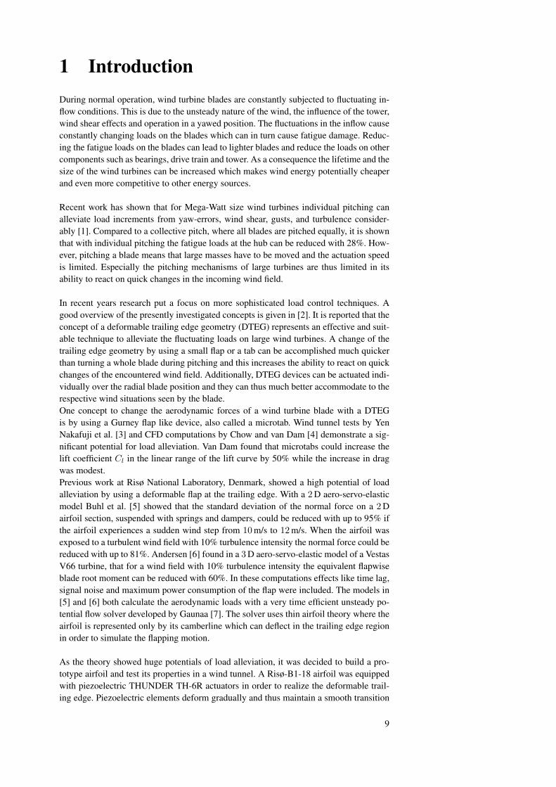
5.2 Harmonic motion of AOA / Fixed flap angleThe prototype airfoil is now tested under a harmonic pitching motion while the flappingangle remains constant at β = 0 ◦. The center of the pitching rotation was placed on thechord line, 0.24 m behind the leading edge. The pitching frequency was chosen to be1.62 Hz which corresponds to a reduced frequency of k = 0.084. The comparisons tothe simulations for four different mean angles of attack are shown in Figures 18 to 21.Additionally the results of potential flow computations using the dynamic stall model byAndersen [9] are shown. The results of the potential flow model are mainly used to con-firm the loop direction of the computed lift and drag loops, they are not part of the generalcomparison between simulations and measurements. For the potential flow simulations ofthis section the computed polars of Figure 15 for the corrected flap at β = 0 ◦ are used asinput.

The lift loops generally fit well in size and shape. The lift loops for αm = −1.55 ◦

and αm = −4.3 ◦ reach slightly lower values whereas the computed lift loops for αm =7.65 ◦ and αm = 11.5 ◦ reach slightly higher values compared to the measurements.These deviations can be explained with the differences in the static lift curves, which arealso shown in the graphs.The lift loops of the CFD computations at αm = −1.55 ◦, αm = 4.3 ◦ and αm = 7.65 ◦

turn counter-clockwise. The exact phase shift is given in the respective graphs where anegative phase angle indicates that the lift lags behind the pitching motion and the liftloop turns counter-clockwise. For αm = 11.5 ◦ the direction of the computed lift loopbecomes clockwise and more opened. This phenomena at high AOA is also discoveredin [8] and can be explained by dynamic stall effects, which cause the flow to not reachits equilibrium state immediately. During pitching towards higher AOA, the separationpoint moves with a certain delay. Compared to the equilibrium state, the separation pointis situated further downstream on the airfoil. This means that larger parts of the flow arestill attached, which then results in a higher lift force. During pitching towards smallerAOA, the delayed movement of the separation point results in less parts of the flow beingattached than in equilibrium. This results in a lower lift force. The measurements do notshow this phenomena. Instead, all lift loops turn clockwise.

All computed drag loops rotate in a clockwise direction. Compared to the measured loops,the range between the maximum and minimum value of Cd is quite high and the loopsdescribe a big open loop. However the mean values of the loops are similar.The loops of the measured Cd values are mostly very narrow and skewed. The recordedlines have several intersections which makes it impossible to determine a distinct loop di-rection. For further investigations of the drag loops, the drag would have to be measuredin a more accurate way.

As the loop directions of the lift loops as well as the shapes of the drag loops show

25

significant differences between CFD simulations and measurements, it was decided touse potential flow results for a final assessment of the results. As seen in the respectivefigures the potential flow calculations confirm the results of the CFD - computations. Thelift loops for αm = −1.55 ◦ and αm = −4.3 ◦ turn counter-clockwise and the shape ofthe drag loops is as open as in the CFD computations. In future wind tunnel tests specialefforts have to be undertaken to figure out if and why the loops show a different behaviourin the test stand.

Figure 18. Pitching around αm = −1.55 ◦, Pitching frequency f = 1.62Hz (k = 0.084),Flap angle β = 0 ◦

Figure 19. Pitching around αm = 4.3 ◦, Pitching frequency f = 1.62Hz (k = 0.084),Flap angle β = 0 ◦

26



27

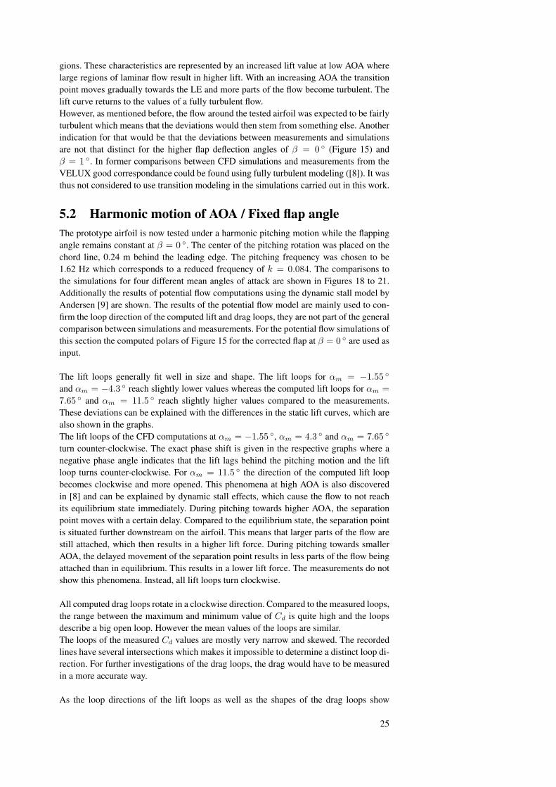
5.3 Fixed AOA / Harmonic motion of flap angleIn the following a harmonic flapping motion is investigated, while the AOA is held con-stant. The measurements and the simulations are compared for the two reduced oscilla-tion frequencies k = 0.081 and k = 0.518. For the test setup this corresponds to thedimensionalized frequencies f = 1.56 Hz and f = 10 Hz. Due to the power limits of theamplifier the flapping angles could not reach the maximum deflection angles of the steadycase. With the strain gauges on the piezoelectric flap the flap angles were monitored. Themeasured flap angles showed a clear dependency on the flapping frequency but no de-pendency on the AOA and the related change in aerodynamic loading. The following flapdeflection angles were measured during the test cases.

- f = 1.56 Hz (k = 0.081): βmin = −3 ◦, βmax = 2 ◦

- f = 10 Hz (k = 0.518): βmin = −2 ◦, βmax = 0.7 ◦

In Figures 22 to 29 the results for the two frequencies at α = −1.3 ◦, α = 4.6 ◦, α = 7.8 ◦

and α = 11.1 ◦ are shown.Again, the shapes of the lift loops fit very well. For the higher AOA of α = 7.8 ◦ andα = 11.1 ◦ the lift loops are located at a slightly higher lift force level. This was alreadyseen in the results of the preceding section and can be explained with the differences inthe steady curves.For all tested AOA the simulated lift loops turn counter-clockwise and the loop shapes donot change significantly. This indicates that even for α = 11.1 ◦ - and thus close to stall -no separation and dynamic stall effects occur. The wind tunnel measurements agree verywell with these observations. All measured lift loops also turn counter-clockwise.

However, it can also be observed that the simulated lift loops reach higher extreme valuesthan their measured equivalents and hence have a steeper slope. Comparing the resultswith the static values which are also shown in the respective figures demonstrate that thedeviations in the extreme values were already present there. It is a consequence of the"bellied" lift curve for low flap deflection angles discussed in Section 5.1 and shown inFigure 17.The slope dCl/dβ is a measure of the lift change potential and thus the efficiency of theflap. Using the extreme values of the lift loops, the following slopes can be determined atthe four observed AOA (Tables 1 and 2).

α = -1.3 ◦ measured: 1.43 rad−1 simulated: 2.35 rad−1

α = 4.6 ◦ measured: 1.34 rad−1 simulated: 2.18 rad−1



Table 1. Flap efficiencies dCl/dβ for f = 1.56 Hz (k = 0.081)

α = -1.3 ◦ measured: 0.95 rad−1 simulated: 1.59 rad−1




Table 2. Flap efficiencies dCl/dβ for f = 10 Hz (k = 0.518)

28

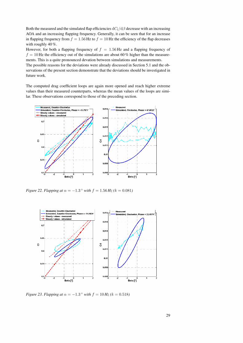
Both the measured and the simulated flap efficiencies dCl/dβ decrease with an increasingAOA and an increasing flapping frequency. Generally, it can be seen that for an increasein flapping frequency from f = 1.56 Hz to f = 10 Hz the efficiency of the flap decreaseswith roughly 40 %.However, for both a flapping frequency of f = 1.56 Hz and a flapping frequency off = 10 Hz the efficiency out of the simulations are about 60 % higher than the measure-ments. This is a quite pronounced devation between simulations and measurements.The possible reasons for the deviations were already discussed in Section 5.1 and the ob-servations of the present section demonstrate that the deviations should be investigated infuture work.

The computed drag coefficient loops are again more opened and reach higher extremevalues than their measured counterparts, whereas the mean values of the loops are simi-lar. These observations correspond to those of the preceding section.

Figure 22. Flapping at α = −1.3 ◦ with f = 1.56 Hz (k = 0.081)

Figure 23. Flapping at α = −1.3 ◦ with f = 10 Hz (k = 0.518)

29

Figure 24. Flapping at α = 4.6 ◦ with f = 1.56 Hz (k = 0.081)

Figure 25. Flapping at α = 4.6 ◦ with f = 10 Hz (k = 0.518)

30



31



32

5.4 Harmonic motion of AOA / Harmonic motion of flapangleFinally the combination of pitching and flapping will be examined. Both the pitching andthe flapping motion have a reduced frequency of k = 0.084 (f = 1.62 Hz). In the windtunnel tests the two oscillatory movements were shifted with a phase shift κ until thevariations in the lift force were minimized. For a phase shift of κ = 0 ◦ the flap reachesits maximum upwrds position at the same time the airfoil reaches its maximum AOA. Apositive phase shift means that the flap motion precedes the pitch motion.Here the results for a mean angle of attack of αm = −1.6 ◦ are discussed. The flap de-flection angle for the chosen frequency varies between β = 2 ◦ and β = −3 ◦.

The wind tunnel tests show the best results for a phase shift of κ ≈ 30 ◦. In the sim-ulations it was not intented to find the optimal phase shift, but several runs with differentphase shifts have been accomplished in order to get a better picture of how the airfoilbehaves for a combined pitching and flapping motion. The results are shown in Figure30 and Figure 31. The measured data and a comparable potential flow simulation areincluded in Figure 30. The results of the measurements could not be confirmed in thesimulation. While in the wind tunnel tests the biggest reductions in lift variation wereachieved for a phase shift of around κ = 30 ◦, the simulations show best results for aphase angle of about κ = 10 ◦.

In the simulations, phase shifts between κ = −50 ◦ and κ = 0 ◦ result in clockwiselift loops, phase shifts between κ = 10 ◦ and κ = 50 ◦ result in counter-clockwise liftloops. However, the measured lift loop at κ = 30 ◦ turns clockwise.

The variation of the computed drag force can be minimized for about the same phaseshift angle of κ = 10 ◦. For phase shift from κ = −50 ◦ to κ = −20 ◦ the drag loopdirection is clockwise. From κ = −10 ◦ to κ = 50 ◦ the loops turn counter-clockwise.However, the measured drag loop at κ = 30 ◦ turns clockwise and thus differently thanthe computed loop.

In order to asses the deviations between measurements and CFD results, potential flowcomputations are used to get a clearer picture of the lift and drag force behaviour during acombined motion in AOA and β. As done in Section 5.2 the potential flow computationsare not discussed in detail here, they are rather used to get an additional indication aboutthe loop directions and loop shapes. The input for the dynamic stall model of Andersen[9] is derived from static lift and drag values of the wind tunnel measurements for severalpitch and flap angles. In Figure 30 the result for a phase shift of κ = 30 ◦ is shown. Thelift and the drag loop of the potential model turn into the same direction as the loops ofthe CFD computations. Additionally, the shapes of the lift and drag loop are also quitesimilar to the CFD computations, although the lift loop of the potential flow computationsis slightly more narrow and the drag loop is slightly more broad. Hence, the potential flowcomputations confirm the results of the CFD simulations. The deviations between sim-ulation and measurement might be consequences of the deviations already stated in theprevious sections.

33

Figure 30. Pitching around αm = −1.6 ◦ Flapping from β = 2 ◦ to β = −3 ◦, f =1.62Hz (k = 0.084), Positive Phase Shifts (10 ◦ ≤ κ ≤ 50 ◦)

Figure 31. Pitching around αm = −1.6 ◦ Flapping from β = 2 ◦ to β = −3 ◦, f =1.62Hz (k = 0.084), Negative Phase Shifts (−50 ◦ ≤ κ ≤ 0 ◦)

6 Further Properties of the AirfoilThe new airfoil model is now used for further steady flow computations. This gives broadinformation about some key properties and the potentials of the prototype airfoil.

First of all the variations of the lift coefficients for several (fixed) AOA and (fixed) flapangles are calculated. This gives information about the general load reduction potential ofthe airfoil. The results are also valuable as input for the dynamic stall model of Andersen[9]. The calculations were carried out for both the corrected flap and the exactly mountedflap.

In Figure 32 the results for the airfoil with the corrected flap position are shown. The

34

values are related to the lift coefficient Cl(β=0) of a non-deformed trailing edge flap (0 Vapplied). It can be seen that the movement of the flap evokes a nearly linear change in lift(holding the AOA constant). The slope dCl/dβ measures the efficiency of the flap, it isthe same quantity that was used in Table 1 and Table 2 for the wind tunnel test compar-isons.It can be seen in the Figure 32, that the efficiency of the flap in the attached flow regionslightly decreases with increasing angles of attack. The maximum flap efficiency occursfor α = −4 ◦ where a slope of dCl/dβ = 2.75 rad−1 is reached. For a flap range ofβ = 2.2 ◦ to β = −5.3 ◦ a ∆Cl of 0.26 is calculated in the steady computations. Fromα = −4 ◦ the efficiency decreases gradually until a dCl/dβ = 1.8 rad−1 at an AOA ofα = 11 ◦.When the flow separates the efficiency of the flap decreases very much. The slope atα = 14 ◦ is only dCl/dβ = 0.65 rad−1. When separation occurs at the aft of the airfoilthe moving flap is not able to bend the flow in the same extend than before. The changein circulation and thus the change in lift decreases.To complete the picture the polars for several flap positions are shown in Figure 34.

Figure 32. Potential of load reduction for the corrected flap

The same investigations are done for the exactly mounted flap which includes the as-sumption that the flap does not change its shape due to aerodynamic forces. In Fig-ure 33 it can be seen that the potential for changing the lift is lower than for the cor-rected flap. The maximum slope at α = −4 ◦ is dCl/dβ = 2.2 rad−1. At α = 11 ◦ it isdCl/dβ = 1.53 rad−1 and at α = 14 ◦ it is dCl/dβ = 0.61 rad−1. The reason for thisdecrease in slope might be the fact that the exact mounted flap is pointing further down.As a consequence the vertical movement of the very tip of the TE is reduced. The camberof the airfoil changes less than for the corrected flap, which reduces the changes in lift.However, the absolute values of the lift coefficients are higher (see Figure 35).

35

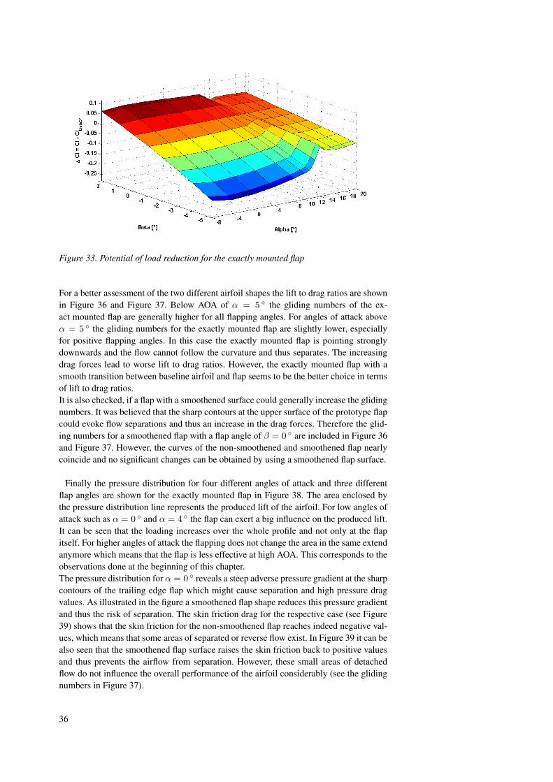
Figure 33. Potential of load reduction for the exactly mounted flap

For a better assessment of the two different airfoil shapes the lift to drag ratios are shownin Figure 36 and Figure 37. Below AOA of α = 5 ◦ the gliding numbers of the ex-act mounted flap are generally higher for all flapping angles. For angles of attack aboveα = 5 ◦ the gliding numbers for the exactly mounted flap are slightly lower, especiallyfor positive flapping angles. In this case the exactly mounted flap is pointing stronglydownwards and the flow cannot follow the curvature and thus separates. The increasingdrag forces lead to worse lift to drag ratios. However, the exactly mounted flap with asmooth transition between baseline airfoil and flap seems to be the better choice in termsof lift to drag ratios.It is also checked, if a flap with a smoothened surface could generally increase the glidingnumbers. It was believed that the sharp contours at the upper surface of the prototype flapcould evoke flow separations and thus an increase in the drag forces. Therefore the glid-ing numbers for a smoothened flap with a flap angle of β = 0 ◦ are included in Figure 36and Figure 37. However, the curves of the non-smoothened and smoothened flap nearlycoincide and no significant changes can be obtained by using a smoothened flap surface.

Finally the pressure distribution for four different angles of attack and three differentflap angles are shown for the exactly mounted flap in Figure 38. The area enclosed bythe pressure distribution line represents the produced lift of the airfoil. For low angles ofattack such as α = 0 ◦ and α = 4 ◦ the flap can exert a big influence on the produced lift.It can be seen that the loading increases over the whole profile and not only at the flapitself. For higher angles of attack the flapping does not change the area in the same extendanymore which means that the flap is less effective at high AOA. This corresponds to theobservations done at the beginning of this chapter.The pressure distribution for α = 0 ◦ reveals a steep adverse pressure gradient at the sharpcontours of the trailing edge flap which might cause separation and high pressure dragvalues. As illustrated in the figure a smoothened flap shape reduces this pressure gradientand thus the risk of separation. The skin friction drag for the respective case (see Figure39) shows that the skin friction for the non-smoothened flap reaches indeed negative val-ues, which means that some areas of separated or reverse flow exist. In Figure 39 it can bealso seen that the smoothened flap surface raises the skin friction back to positive valuesand thus prevents the airflow from separation. However, these small areas of detachedflow do not influence the overall performance of the airfoil considerably (see the glidingnumbers in Figure 37).

36

Figure 34. Polars for for several flapping angles (corrected flap)

37

Figure 35. Polars for for several flapping angles (exactly mounted flap)

38

Figure 36. Gliding numbers for the corrected flap

Figure 37. Gliding numbers for the exactly mounted flap

39

α = 0◦ α = 4◦

α = 8◦ α = 12◦

Figure 38. Pressure distributions for several AOA and flap angles

Figure 39. Skin friction coefficient at α = 0 ◦ for the smoothened and normal flap surface

40

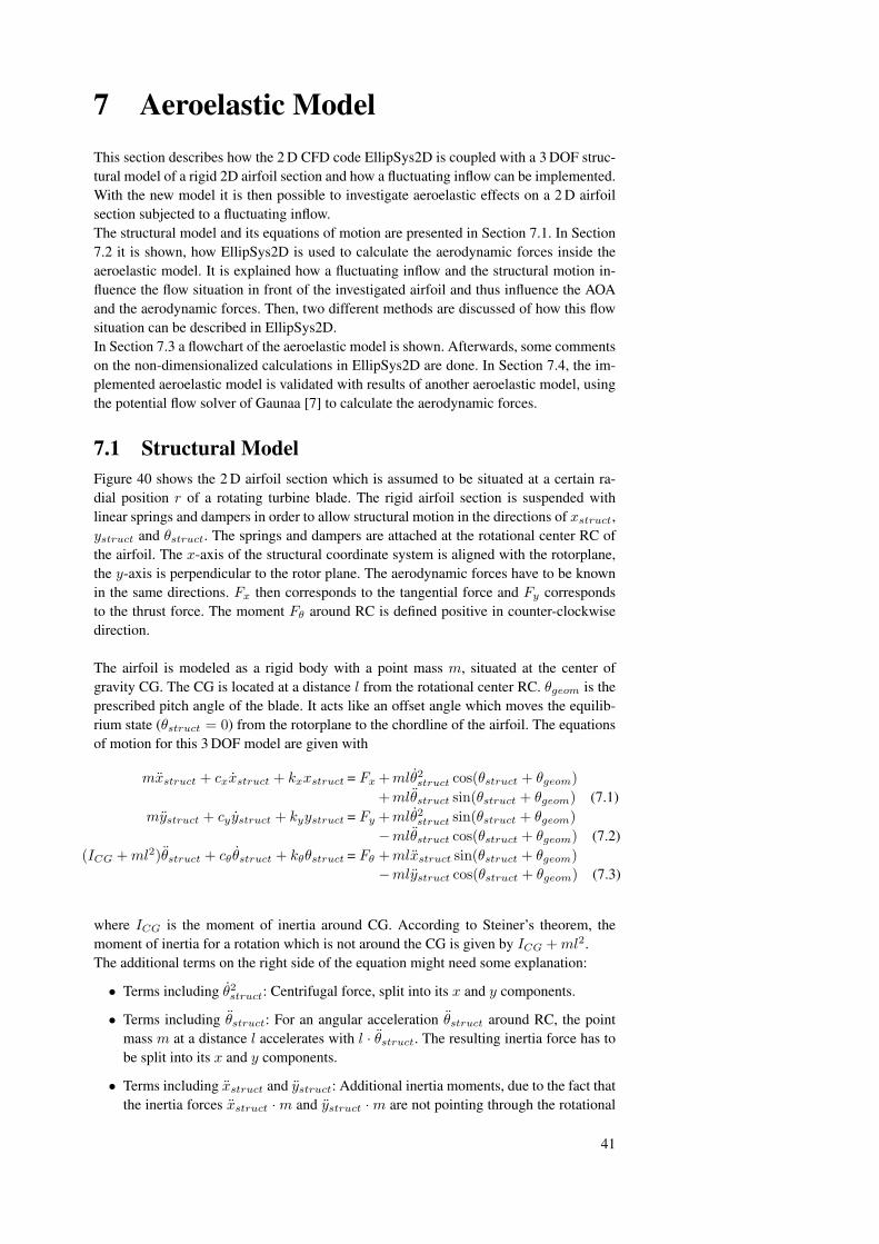
7 Aeroelastic ModelThis section describes how the 2 D CFD code EllipSys2D is coupled with a 3 DOF struc-tural model of a rigid 2D airfoil section and how a fluctuating inflow can be implemented.With the new model it is then possible to investigate aeroelastic effects on a 2 D airfoilsection subjected to a fluctuating inflow.The structural model and its equations of motion are presented in Section 7.1. In Section7.2 it is shown, how EllipSys2D is used to calculate the aerodynamic forces inside theaeroelastic model. It is explained how a fluctuating inflow and the structural motion in-fluence the flow situation in front of the investigated airfoil and thus influence the AOAand the aerodynamic forces. Then, two different methods are discussed of how this flowsituation can be described in EllipSys2D.In Section 7.3 a flowchart of the aeroelastic model is shown. Afterwards, some commentson the non-dimensionalized calculations in EllipSys2D are done. In Section 7.4, the im-plemented aeroelastic model is validated with results of another aeroelastic model, usingthe potential flow solver of Gaunaa [7] to calculate the aerodynamic forces.

7.1 Structural ModelFigure 40 shows the 2 D airfoil section which is assumed to be situated at a certain ra-dial position r of a rotating turbine blade. The rigid airfoil section is suspended withlinear springs and dampers in order to allow structural motion in the directions of xstruct,ystruct and θstruct. The springs and dampers are attached at the rotational center RC ofthe airfoil. The x-axis of the structural coordinate system is aligned with the rotorplane,the y-axis is perpendicular to the rotor plane. The aerodynamic forces have to be knownin the same directions. Fx then corresponds to the tangential force and Fy correspondsto the thrust force. The moment Fθ around RC is defined positive in counter-clockwisedirection.

The airfoil is modeled as a rigid body with a point mass m, situated at the center ofgravity CG. The CG is located at a distance l from the rotational center RC. θgeom is theprescribed pitch angle of the blade. It acts like an offset angle which moves the equilib-rium state (θstruct = 0) from the rotorplane to the chordline of the airfoil. The equationsof motion for this 3 DOF model are given with

mxstruct + cxxstruct + kxxstruct = Fx +mlθ2struct cos(θstruct + θgeom)+mlθstruct sin(θstruct + θgeom) (7.1)

mystruct + cy ystruct + kyystruct = Fy +mlθ2struct sin(θstruct + θgeom)−mlθstruct cos(θstruct + θgeom) (7.2)

(ICG +ml2)θstruct + cθ θstruct + kθθstruct = Fθ +mlxstruct sin(θstruct + θgeom)−mlystruct cos(θstruct + θgeom) (7.3)

where ICG is the moment of inertia around CG. According to Steiner’s theorem, themoment of inertia for a rotation which is not around the CG is given by ICG +ml2.The additional terms on the right side of the equation might need some explanation:

• Terms including θ2struct: Centrifugal force, split into its x and y components.

• Terms including θstruct: For an angular acceleration θstruct around RC, the pointmass m at a distance l accelerates with l · θstruct. The resulting inertia force has tobe split into its x and y components.

• Terms including xstruct and ystruct: Additional inertia moments, due to the fact thatthe inertia forces xstruct ·m and ystruct ·m are not pointing through the rotational

41

center.

The same structural model was used in the work of Buhl et al. [5] and the work of Ander-sen [6], the only difference is that the signs of the rotational angles θgeom and θstruct havebeen changed to conform to the right hand rule and the sign conventions of EllipSys2D.

The aerodynamic forces Fx, Fy and Fθ are taken out of the CFD calculations (see Section7.2). Knowing the aerodynamic forces and the respective structural deflections xstruct,ystruct and θstruct and velocities at a certain time step n, the equations (7.1) - (7.3) areused to calculate the structural deformations at the next time step n+ 1. This is done byusing the Runge-Kutta-Nyström integration scheme.

Figure 40. Notations and directions of the Structural model

7.2 Aerodynamic ModelEllipSys2D is used to calculate the aerodynamic forces generated by the investigated air-foil. During the aeroelastic simulation, the airfoil is subjected to a fluctuating inflow andto a certain movement due to structural deflections. Both the fluctuating inflow and thestructural motion change the AOA for the investigated airfoil section and thus change theaerodynamic forces. In this section it is discussed how these influences can be describedin EllipSys2D. Two different possibilities of realizing the fluctuating inflow are presentedand their advantages and disadvantages are mentioned.Before discussing these two possibilities in Section 7.2.2, some general definitions andterms are introduced in Section 7.2.1 which describe the simulated flow situation in frontof the considered 2D airfoil section.

7.2.1 Flow situation in front of the airfoil

Flow situation excluding structural motion:

Corresponding to Figure 40, we observe a 2D airfoil section which is situated at a certainradial position r of a rotating turbine blade. If no structural deformations are taken intoaccount, the angles and wind velocity components in front of the airfoil can be defined asillustrated in Figure 41.Assuming that the wind direction is perpendicular to the rotor plane, the wind can be

42

described by the axial velocity Va. Due to the rotational velocity of the blade at the con-sidered radius r, an additional rotational velocity component Vrot has to be considered.These two velocity components add up to the relative velocity Vrel and the angle betweenVrot and Vrel is then defined as the flow angle φpresc. In case of a wind gust or a fluc-tuating inflow, this flow angle φpresc changes over time, because the wind velocity Vachanges over time.The pitch angle θgeom is the angle from the rotorplane to the chordline. Pitching the bladeis reducing (or increasing) the AOA and thus regulating the aerodynamic forces producedby the airfoil.The resulting AOA αpresc is:

αpresc = φpresc − θgeom with φpresc = tan(−1)Vrot

Va(7.4)

In Equation (7.4) the flow angle and the AOA have the subscript presc. This is becausethe axial wind velocity Va, the rotational speed of the blade Vrot as well as the pitch angleθgeom will be known in advance in the upcoming EllipSys simulations. This means thatthe resulting flow angle φpresc and the AOA αpresc are prescribed by that input. As soonas the computed and thus non-prescribable structural motion is added, the flow angle andAOA will change respectively and the subscript presc will be dismissed.

Figure 41. Definition of the angles and wind velocity components for a 2D airfoil section(structural motion excluded)

Flow situation including structural motion

In Figure 42 it is now shown, how an additional structural motion of the airfoil affects theAOA. As mentioned in Section 7.1 the structural motion in x is aligned with the rotor-plane, the structural motion in y is perpendicular to the rotor plane. It is illustrated, howthe velocity components xstruct and ystruct add up to the axial and rotational velocityand thus form the new flow angle φ. The structural motion θstruct around the rotationalcenter RC adds up to the pitch angle θgeom and the new AOA α can be described withthe formula:

α = φ− (θgeom + θstruct) with φ = tan(−1)Vrot−xstruct

Va−ystruct(7.5)

43

Figure 42. Definition of angles and wind velocity components for a 2D airfoil section(structural motion included)

7.2.2 Describing the Flow Situation in EllipSys2D

As mentioned in Section 2.1, EllipSys2D provides five different variables, rx, ry , ϕ,uinlet and vinlet, in order to adjust the AOA of the airfoil. This gives several possibilitiesto describe the flow situation of Figure 42.

In this section two different methods of describing the fluctuating inflow (and thus theprescribed flow angle φpresc) are discussed. The first method uses the variable uinlet andvinlet, the second method uses the variable ϕ to describe φpresc. The advantages and dis-advantages of the two methods will be pointed out and finally one method will be chosenfor the upcoming simulations.

Method 1: Using uinlet and vinlet to describe φpresc:

This method is quite intuitive and seems to be easy. As illustrated in Figure 43 the changein the prescribed flow angle φpresc is accomplished by changing the inlet velocity com-ponents uinlet and vinlet according to Vrot and Va.Changes in θgeom and θstruct can be realized by rotating the grid withϕ = θgeom + θstruct.Remember from Figure 1 that a rotation in ϕ does not change the orientation of the CFDcoordinate system. This means that during the whole simulation the coordinate systemof EllipSys2D (in which the aerodynamic forces are calculated) is aligned with the co-ordinate system of the structural motion (in which the structural deflection is calculated)which is the big advantage of this method.Due to the aligned coordinate systems the structural motions xstruct and ystruct out ofthe structural model do not have to be rotated and can simply be used for rx and ry insideElipSys2D. The same can be said about the forces F ∗x,CFD and F ∗y,CFD out of the CFDcalculations. They can be used inside the structural model without any rotational trans-formation.

The input to EllipSys2D would be:

uinlet = V ∗rot; vinlet = V ∗a ; rx = x∗struct; ry = y∗struct

ϕ = θgeom + θstruct

44

The input to the structural model would be:

Fx = F ∗x,CFD · fdim,f ; Fy = F ∗y,CFD · fdim,f ; Fθ = F ∗θ,CFD · fdim,m

where the ∗ stands for a non-dimensionalized quantity. fdim,f and fdim,m are dimen-sionalization factors. (See Appendix A for more information on the non-dimensionalizedquantities used in EllipSys2D)

Figure 43. Flow angle φpresc defined via uinlet and vinlet

But there are several drawbacks of this method. EllipSys2D is an incompressible flowsolver. Thus, at every time step, the mass flux into the computational domain has to beequal to the mass flux out of the domain in order to fulfil the global mass conservation.Changing the inlet velocities uinlet and vinlet due to a fluctuating inflow means that themass flux into the domain is changing continuously. In reality a change in the inflowvelocity needs some time to travel downstream and influence the flowfield around andbehind the airfoil. However, in incompressible CFD computations the mass flux at theoutlet has to be immediately adapted to the change in inflow in order to maintain globalmass conservation. This means that an increase in the inflow velocity results in an im-mediate and thus unphysical increase of the outlet velocity. As a consequence the wholeflow field inside the computational domain is jumping to a higher velocity level which isnot physical either. A possibility to overcome this problem is to continuously scale thechanging inflow velocities in order to keep the total mass flux constant.A second drawback is the problem of timing. Using an O-mesh around the airfoil theinlet boundaries are located in an oval arc around the airfoil (see Figure 1) and thus eachinlet cell varies in its x and y coordinates. In order to describe a uniform fluctuation inthe velocity components of x and y (i.e. u and v) the inlet velocities have to be altered ina certain time sequence.Due to these rather laborious changes it was decided to look for an easier possibility toimplement the fluctuating inflow.

Method 2: Using ϕ to describe φpresc:

This method is illustrated in Figure 44. The change in the flow angle φpresc is now ac-complished by rotating the movable mesh of EllipSys2D with ϕφ = −φpresc while theinlet direction defined via uinlet is kept constant (vinlet = 0). This means that the inlet

45

velocity remains perpendicular throughout the whole computation (see Figure 1). In or-der to obtain the same flow situation as in Figure 42 the CFD coordinate system has to berotated with φpresc.Changes in θgeom and θstruct are realized by rotating the mesh with ϕθ = θgeom+θstructand the overall rotation of the movable mesh is then given with ϕ = ϕφ + ϕθ =−φpresc + θgeom + θstruct.

Figure 44. Flow angle φpresc defined via ϕ

The rotation of the CFD coordinate system complicates the problem, since the structuralmotions xstruct and ystruct have to be rotated by the angle φpresc before they can beused inside EllipSys. The same holds for the aerodynamic forces Fx,CFD∗ and Fy,CFD∗out of EllipSys2D. They have to be rotated by the angle −φpresc before they can be usedinside the structural model.

The input to EllipSys2D is then:

uinlet =√V ∗rot

2 + V ∗a2 != 1

vinlet = 0rx = x∗struct cosφpresc + y∗struct sinφprescry = y∗struct cosφpresc − x∗struct sinφprescϕ = −φpresc + θgeom + θstruct (7.6)

The input to the structural model is then:

Fx = (F ∗x,CFD cosφpresc − F ∗y,CFD sinφpresc) · fdim,fFy = (F ∗x,CFD sinφpresc + F ∗y,CFD cosφpresc) · fdim,fFθ = F ∗θ,CFD · fdim,m (7.7)

where the ∗ stands for a non-dimensionalized quantity. fdim,f and fdim,m are dimen-sionalization factors. (See Appendix A for more information on the non-dimensionalized

46

quantities used in EllipSys2D)

Changing the inflow by rotating the airfoil does not fully correspond to the real case.In reality a change in the wind field in front of the airfoil needs some time to travel downthe airfoil. In the simulation, due to the rotation of the airfoil, the change in the windvelocity is felt imediately at all positions of the blade. However, this withdraw of method2 is assumed to have minor effects on the computed forces. A respective investigation ofthis is mentioned in [5] using potential flow theory. On the other hand, by using method 2the difficulties of implementing method 1 can be circumvented and it is therefore decidedto use method 2 for the aeroelastic modeling in this work.

7.3 Flowchart of the aeroelastic model

Figure 45. Coupling between EllipSys2D and structural model

In Figure 45 it is shown, how EllipSys2D is coupled with the structural model. At eachtime step of the CFD computations, the AOA α as well as the flap angle β have to be de-termined in order to calculate the correct aerodynamic forces. The AOA α is adjusted by

47

using the equations of (7.6). The prescribed flow angle φpresc is read out of a file calledpresc.inflow. The file contains a time series of the flow angle φpresc which correspondsto the desired inflow situation (wind gust or turbulent wind field). The pitch angle θgeomis a fixed given value. x∗struct, y

∗struct and θ∗struct are given by the structural model. As

long as no control is implemented, a fixed flap angle β is used.After the resulting flowfield is computed, the forces F ∗x,CFD, F ∗y,CFD as well as the mo-ment F ∗θ,CFD around RC are determined and given to the structural model.In the structural model, the aerodynamic forces are dimensionalized and rotated intothe structural coordinate system (see equation (7.7)). The forces are then used insidethe equations (7.1) - (7.3) in order to calculate the structural displacements at the nexttime step with the Runge-Kutta-Nyström scheme. The structural deflections are non-dimensionalized before they are given back to EllipSys.

7.4 Validation of the ModelValidation of the time integration scheme:

First, the correct implementation of the Runge-Kutta-Nyström time integration scheme ischecked. This is done by solving the 2nd order ordinary differential equation

mx+ kx = F0 cos (ωt) (7.8)

which describes the response x of a 1 DOF system, suspended on a spring k and subjectedto a harmonic external load F0. No damping is included.For equation (7.8) an exact, analytical solution exists which can be compared with thesolution of the Runge-Kutta scheme. The analytical solution is given by

x(t) =F0

m(ω20 − ω2)

cos (ωt) + (x0 −F0

m(ω20 − ω2)

) cos (ω0t) +x0

ω0sin (ω0t)

where ω0 =√k/m is the natural frequency of the system and x0, x0 are the initial

conditions of the system.In Figure 46 the two solutions for F0 = 10 N, m = 1 kg, k = 100 N/m, ω = 5 s−1 andthe initial conditions x0 = 0 m, x0 = 0 m/s are compared to each other. The computedpositions, velocities and accelerations coincide very well.

Time step in the structural model

The input parameters of the validation case are chosen such that the magnitudes of posi-tion, velocity and acceleration are comparable to what can be expected in later aeroelasticcomputations. Normally, it has to be investigated which time step is suitable to capturethe fluctuations in x accurately. But here the time step of the Runge-Kutta scheme is notconsidered to be critical as it is coupled with the time step of EllipSys2D. Using the non-dimensional time step of ∆t∗ = 0.01 in EllipSys2D (see Chapter 4), the correspondingtime step in the Runge-Kutta scheme is ∆t = 0.00017 s (see equation (A.11) for c = 1 mand U∞ = 60 m/s) which is small enough to resolve any kind of physical motion of theairfoil section. In Figure 46 a time step of ∆t = 0.00017 s is used.

Validation of the aeroelastic model:

The 3 DOF aeroelastic model is now compared to another aeroelastic model, which usesthe potential flow solver of Gaunaa [7] and the dynamic stall model of Andersen [9] tocalculate the aerodynamic forces. For the comparison the Risø B1-18 baseline airfoil isused where no flap is attached. At t = 1 s the airfoil is exposed to a wind gust which

48

Figure 46. Comparison between the analytical and numerical solution (F0 = 10 N,m = 1 kg, k = 100 N/m, ω = 5 1/s, ∆t = 0.00017 s

corresponds to a step change in the axial wind velocity Va from 10 m/s to 12 m/s. Therotational velocity remains at 60 m/s. The air density is ρ = 1.225 kg/m3. The rotationalcenter RC and the center of gravity CG are both assumed to be situated on the chordlineof the airfoil. All quantities used in the structural model are listed in Table 3. Structuraldamping is neglected. The time step is ∆t∗ = 0.01 or ∆t = 0.00017 s

Table 3. Structural quantities used in this work

RC (distance from LE) 0.30 mCG (distance from LE) 0.35 mm (per unit depth) 40 kgkx 6316 N/mky 1579 N/mkθ 8290 N/radcx, cy, cθ 0 Ns/mθgeom 5 ◦

The two calculations are compared in Figures 47 and 48. The time line in these figuresstarts at t = 0 s but the simulations were already started at t = −3 s in order to reach astructural equilibrium position before the step change in wind takes place. However, theoscillations in the (nearly) edgewise direction xstruct damp out very slowly and are stillpresent at t = 0 s.In Figure 47 it can be seen that the calculated structural deflections xstruct, ystruct andθstruct of the two models fit excellently together. Both the absolute values and the dy-namic behaviour are nearly identical. In the results for ystruct it can be seen that thecurve out of the CFD computation shows a somewhat softer or delayed reaction to thesimulated step change. This slight delay can also be seen in the results for θstruct. Thereason for that is that the wind step in EllipSys2D can not be simulated with an immedi-ate change and the maximum change in the wind velocity Va has to be limited in orderto omit unrealistic transient forces which evoked very high and unrealistic oscillations inθstruct and ystruct. (see Appendix B for more information).The comparison of the normal and tangential force coefficients Cn and Ct in Figure 48shows a very good correlation as well. However, some differences can be pointed out

49

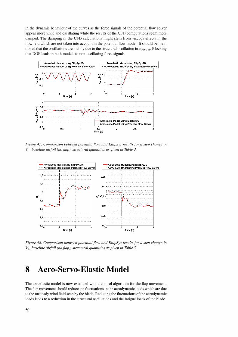
in the dynamic behaviour of the curves as the force signals of the potential flow solverappear more vivid and oscillating while the results of the CFD computations seem moredamped. The damping in the CFD calculations might stem from viscous effects in theflowfield which are not taken into account in the potential flow model. It should be men-tioned that the oscillations are mainly due to the structural oscillation in xstruct. Blockingthat DOF leads in both models to non-oscillating force signals.

Figure 47. Comparison between potential flow and EllipSys results for a step change inVa, baseline airfoil (no flap), structural quantities as given in Table 3

Figure 48. Comparison between potential flow and EllipSys results for a step change inVa, baseline airfoil (no flap), structural quantities as given in Table 3

8 Aero-Servo-Elastic ModelThe aeroelastic model is now extended with a control algorithm for the flap movement.The flap movement should reduce the fluctuations in the aerodynamic loads which are dueto the unsteady wind field seen by the blade. Reducing the fluctuations of the aerodynamicloads leads to a reduction in the structural oscillations and the fatigue loads of the blade.

50

In this work two different control strategies are implemented. Control 1 is using the AOAαmeas measured in front of the airfoil as input. Control 2 is using the pressure difference∆pmeas between the pressure and suction side at a certain chord position as input. Thetwo controls were implemented in this model as they promise a high reduction potentialof the fatigue loads (see Reference [5] and [19]).

8.1 Control 1This control uses the AOA in front of the airfoil as input. The inflow angle can for instancebe measured with a 5-hole pitot tube which measures the AOA in a certain distance d1 infront of the LE (see Figure 49). A change in the measured AOA indicates that the lift forceis changing and the control then tries to counteract the lift change by actuating the flapadequately. Previous simulations with a potential flow solver showed that the potential ofload reduction with a control using the AOA as input was higher than with a control usingthe structural deflection ystruct and/or velocity ystruct as input ([5]).

The control algorithm is given by:

β = (2π

Hdydx(αmeas − αref )) ·Aα + βm (2)

where αmeas is the AOA measured with the pitot tube. Aα is the gain parameter of thecontrol and αref denotes the integral term

αref =1τ

∫ t

t−ταmeas(t) dt (3)

which is the average value of αmeas during a reference time window τ .

This control algorithm is based on the algorithm found in [5]. It aims at keeping the actualAOA αmeas close to the reference value αref and deviations between those two valueslead to a change in β (see equation (2)). The parameter Hdydx represents the potentialof the airfoil to change the lift via flapping. It corresponds to the slope dCl/dβ which inChapter 6 was described as the effectiveness of the flap.Hdydx is used to relate the devia-tion between αmeas and αref to a reasonable change in the flap deflection angle β whichcounteracts the change in lift. The parameter depends on α and β, but in the followingcomputations this dependency is neglected and an average value of Hdydx = −2rad−1

is used. However, the gain parameter Aα is used to fine tune the efficiency of the control.The computed change in β is then added to the middle position βm of the flap. Thus thecontrol always orients at the middle position and ensures that the flap can react to bothsides into the same extent.The calculations in Chapter 9 are carried out assuming a pitot tube length of d1 = 0.3 · c.

Figure 49. Control 1: Pitot tube attached at d1 in front of the LE

51

Getting αmeas out of EllipSys2D:

In EllipSys2D the pitot tube in front of the LE is not modeled as a solid body, insteadit was decided to simply extract the velocity components u and v at a certain point/cellin front of the airfoil. The model is thus neglecting the influence of the pitot tube on theflow field in front of the airfoil, however, this influence is considered to be very modest.In order to ensure that the velocity extraction point stays at a fixed distance to the airfoil,it has to be located inside the rigid part of the moving mesh.The extracted velocity components uextr and vextr are given in the directions of the CFDcoordinate system. In Figure 50 it is shown that the corresponding angle αextr is the anglebetween the x axis of the CFD coordinate system and Vrel. But the desired AOA αmeasis defined as the angle between the chordline of the airfoil and Vrel. As soon as the airfoiland thus the moving mesh is rotated by a certain angle ϕ (refer to Figure 1), the chordlinedeviates from the x axis of the CFD coordinate system and the additional rotation has tobe considered. This leads to the expression of

αmeas = αextr − ϕ = atan(vextr/uextr)− ϕ (4)

Figure 50. Getting αmeas out of EllipSys2D

8.2 Control 2This control uses the pressure difference ∆pref at a certain point between pressure andsuction side as input. As seen in Figure 51, pressure taps were mounted at a distanced2 from the LE in order to determine the pressure difference. A change in the measuredpressure difference indicates a change in the aerodynamic loading and the control thentries to counteract by actuating the flap in order to keep the pressure difference close toa certain reference value. Previous aero-servo-elastic simulations using a potential flowsolver for the aerodynamic modeling promised a big potential in load alleviation for thiscontrol ([19]).

The control algorithm is given with:

β = (∆pmeas −∆pref ) ·Ap + βm (5)

where ∆pmeas is the measured pressure difference between the upper and lower pressuretap. Ap is the gain parameter of the control and ∆pref denotes the integral term

52

∆pref =1τ

∫ t

t−τ∆pmeas(t) dt (6)

which is the average value of ∆pmeas during a reference time window τ .

In equation (5) it can be seen that deviations between the two values will lead to a changein β. It is the task of the gain parameter Ap to translate this change in pressure into areasonable change of the flap deflection angle. In difference to (4) the gain of control2 is a dimensionalized quantity as a corresponding prefactor to 2π/Hdydx has not beendetermined yet in previous work.The resulting change in β is added to the flap deflection angle βm which should be themiddle position between βmax and βmin. The control returns to that middle position ifno change in β is needed (∆pmeas is equal to ∆pref ) and maintains the possibility thatthe flap can react to both sides in the same extend.The calculations in Chapter 9 are carried out with pressure taps located at d2 = 0.12 · cas computations using a potential flow solver showed good results at this measurementposition of the Risø B1-18 airfoil. A favoured position for the pressure taps is supposedto be located where a change in lift evokes distinct changes in ∆pmeas and the optimumpoint might thus change if another airfoil than the Risø B1-18 is chosen.

Figure 51. Control 2: Pressure taps at d2 to measure the pressure difference

Getting ∆pmeas out of EllipSys2D:

The pressure taps are measuring the pressure on the airfoil surface at a given distance d2

from the leading edge. A little routine inside the EllipSys code is identifying the two sur-face cells of the pressure and suction side which are located closest to the given distanced2. The read out cp values are then translated to the dimensionalized pressure difference

∆pmeas = (cp(up) − cp(down)) ·12ρU2∞ (7)

using the freestream dynamic pressure to dimensionalize.

8.3 Reference Time WindowThe values ∆pref and αref are used as reference values inside the control algorithms.These values are a kind of optimum value and the control reacts as soon as the state vari-ables αmeas or ∆pmeas deviate from these references. The optimum values are definedby averaging previous values over a certain time window τ (see equation (6) and (3)). Toget an effective control, it is important to choose an adequate reference time τ .

53

• Choosing a very long time window τ will lead to slow changes in the optimal valuesand the control will try to even cancel out very slow variations in ∆p (Control 1)or AOA (Control 2). An example for slow variations could be the change in ∆p orAOA due to a change in wind speed from 5 m/s 25 m/s. A long time window wouldkeep the reference values close to the values measured at 5 m/s, and the flap wouldtry to alleviate these big changes in the aerodynamic loading. But it makes no senseand is just impossible to alleviate these variations with the flap.

• Choosing a very short time window τ will lead to quick changes in the optimal val-ues. Small fluctuations in the aerodynamic loading, due to turbulences in the wind,might not be filtered out as much as desired.

According to previous work the time window reference is chosen to be τ = 6 s. This cor-responds to 1 full blade rotation of a 10MW turbine. Variations which are slower thanthis 1P period are expected to be regulated by the pitch control. All quicker fluctuationsin the wind field and thus in the aerodynamic forces should then be alleviated by the flap.

8.4 Maximum Actuation Velocity, Maximum Flap An-gles, Time DelayMaximum Actuation Velocity

The piezoelectric flaps have some limitations on their actuation velocity. Out of experi-ments the flap needs approximately 1/100 s to get from β = 2, 2 ◦ to β = −3 ◦ (flappingup) while it needs approximately 4/100 s to get from β = −3 ◦ to β = 2, 2 ◦ (flappingdown). Neglecting acceleration and deceleration effects this gives a maximum actuationvelocity of −520 ◦/s and +130 ◦/s respectively. The maximum deflection angles pertime step ∆t of the aero-servo-elastic computations are thus

∆βmax,down = −520 ◦/s ·∆t ; ∆βmax,up = 130 ◦/s ·∆t (8)

In case the desired ∆β of the control algorithm is bigger then the one given in equation(8), the desired value is overwritten and the maximum value is used instead.

Maximum Flap Angles

The maximum flap deflection range is set to 2.2 ◦ ≤ β ≤ −5.3 ◦. This correspondsto the maximum static deflection which could be reached with the prototype. Furtherrestrictions on the maximum flapping range which occurred during the wind tunnel testsare not considered here, as they were due to the limitations of the used amplifier (seeChapter 5).

Time Delay

In order to make the computations more realistic a certain time delay tdelay can be intro-duced to the computations. This time delay accounts for the time needed to receive thesignal from the measurement device, process it in the control and to finally put the re-sponse signal to the flap actuator. Former investigation in [5] and [6] showed that the loadreduction potential of the flap control is very much influenced by time delays. Thus it wasconsidered to be important to include a time delay investigations to the present work. Thetime delay is realized by a simple time shift inside the code. This means that the controlalgorithm uses measured state variables which stem from the time t = tnow − tdelay.

54

8.5 Flowchart of the Aero-Servo-Elastic ModelThe implementation of the control into the existing aero-elastic model of Chapter 7 isshown in Figure 52. The flap deflection angle β is taken out of the control algorithmwhich uses the extracted values cp(up) and cp(down) or αextr of the previous time stepas input. The corresponding ∆pmeas and αmeas are then calculated with equation (7) or(4). After determine the respective reference values (equation (6) or (3)) and introducinga possible time delay, the respective control algorithm is solved in order to determine thedesired new flap angle β. Finally it is checked if the desired flap movement has to belimited due to the restrictions of the maximum flapping velocity.The grid of the new airfoil shape is then generated with a linear interpolation between the

Figure 52. Flowchart of the aero-servo-elastic Model

55

maximum grids for βmin = −5.3 ◦ and βmax = 2.2 ◦ (as explained in Chapter 2.2).

9 Results of Test CasesThe 2D airfoil section equipped with the piezoelectric flap is now exposed to differentwind situations and its ability to reduce the fatigue loads is investigated. The reduction ofthe fatigue loads is measured by comparing the respective standard deviations Std(y) ofthe structural deflections in ystruct (see Section 9.1).For both controls several gain parameters are tested in order to obtain information aboutthe optimal gain values and the respective reduction potential in Std(y). These investiga-tions are first carried out for a step change in wind from Va = 10 m/s to Va = 10.5 m/s(Section 9.2), then the same investigations are done for a 4 seconds turbulent wind fieldsignal with TI = 2.2% (Section 9.3). Additionally, the same turbulent inflow is used toexamine the control’s dependency on possible time delays inside the control loop.In the last two sections results of longer simulation runs are shown. Using the optimalgain values determined in the previous section and assuming no time delay in the controlloop, the two controls are used to alleviate the structural deflections in ystruct evokedby a 12 seconds turbulent windfield signal. Both a turbulent wind field with TI = 2.4%(Section 9.4) and a turbulent wind field with TI = 7.7% (Section 9.5) is simulated. To al-leviate the fluctuations of the wind field with TI = 7.7% the controls seek for higher flapdeflection angles than the actual maximas of βmin = −5.3 ◦ and βmax = 2.2 ◦. There-fore the last simulation is carried out with extended flap deflection limits of βmin = −6 ◦

and βmax = 6 ◦ in order to demonstrate the load reduction potential using future piezo-electric actuators as deformable TE flaps.

In the simulations of this chapter the DOF in xstruct is blocked as for the relatively shortsimulation runs the oscillations in xstruct are mainly related to the chosen initial condi-tions and not to any aerodynamic effects. Thus the oscillations in xstruct do not effectthe conclusions about the load reduction potential of the flap. Additionally the reductionpotential is determined via the standard deviation Std(y) in ystruct which is likewise notaffected significantly by blocking the structural motion in xstruct.

To achieve comparable starting conditions for the several test cases the computationswere started a certain time before t = 0 s. Thereby the equilibrium state of ystruct andθstruct is reached and the computations start from a settled flow field around the airfoil.In C a typical input file of EllipSys is shown which inter alia gives detailed informationabout the chosen time sequence of a typical simulation. Additionally, information aboutthe required computational time is given there.

9.1 Definition of Std(y) and reduction potential RStd(y)

The implemented control algorithms aim to reduce the fluctuations in the aerodynamicloads and thus reduce the associated fatigue loads on a wind turbine blade subjectedto a fluctuating wind field. Compared to the fluctuations in drag the changes in the liftforce are much more pronounced. Additionally, the lift force acts mainly into the flapwiseblade direction where the blade stiffness is lowest. The highest variations in the structuraldeformations are thus expected in the flapwise blade direction which is in turn close tothe y-direction of the structural coordinates (see Figure 40).It is therefore decided to compare the implemented control algorithms by comparing therespective standard deviations Std(y) of the structural deformation ystruct. The lower theStd(y) the less the airfoil is oscillating in the flapwise direction and the less the blade isexposed to fatigue damage. Std(y) is calculated by

56

Std(y) =

√√√√ N∑i=1

1N

(ystruct(i) − ystruct)2 (9)

where N is the total number of time steps and ystruct is the mean deflection of the ob-served time period.During the simulation of a wind step ystruct is set to the deflection which is found beforethe wind step occurs. The optimum result of Std(y) = 0 m is thus achieved when ystructcan be held on the same level as before the wind step.

The reduction potential RStd(y) of a given control algorithm is computed by setting theStd(y) of the non-controlled case to 100%. Thus the reduction potential of the controlledcase is given in [%] and calculated by

RStd(y) =(Std(y)uncontrolledStd(y)controlled

− 1)· 100 (10)

9.2 Airfoil exposed to wind stepFirst, the airfoil is exposed to a wind step in which the axial wind velocity Va (see Figure42) changes from 10 m/s to 10.5 m/s at t = 0.5 s. A wind step can be considered asthe elementary case of any wind signal and gives easy interpretable results. The gainparameters which relate the change in the measured state variable to a suitable movementof the flap can be conveniently determined.The maximum rate of change in φpresc was limited to 40 ◦/s in order to omit unrealistictransient forces in the EllipSys computations (see Appendix B for more information).

Control 1

As mentioned in Section 8.1 the pitot tube is assumed to measure αmeas at a distanced1 = 0.3 · c in front of the airfoil. In Figure 53 the resulting deflection ystruct is shownfor different gain parameter Aα. The time delay is set to tdelay = 0.0s.Gain parameters in the range of 0.50 ≤ Aα ≤ 0.80 and with an interval of ∆Aα = 0.05

Figure 53. Structural deflection in ystruct during a wind step from Va = 10 m/s toVa = 10.5 m/s, Control 1.

are investigated. The respective reduction in the standard deviation Std(y) are given in

57

the graph and the best reduction can be achieved with a gain of Aα = 0.65 where theStd(y) can be reduced with RStd(y) = 98 %.The simulation for Aα = 0.65 is now observed in more detail. The corresponding flapangles β and the normal force Fy are shown in Figure 54. It can be seen how β, after somesmall oscillations, reaches its new equilibrium value of approximately −3.5 ◦ in order tohold Fy unchanged at a value slightly above 2800 N.In Figure 55 the AOA at two different distances to the LE are shown. Both graphs show

Figure 54. Flap angle β and normal force Fy during a wind step from Va = 10 m/s toVa = 10.5 m/s, Control 1, Aα = 0.65

Figure 55. αmeas at d1 = 0.3 · c (up) and α at 10 · c (down) for the uncontrolled andcontrolled case, Control 1, Aα = 0.65,

the uncontrolled and the controlled response for Aα = 0.65 and d1 = 0.3 · c. In the uppergraph the AOA at a distance of 0.3 · c in front of the LE is illustrated. Below, the AOAat 10 · c for the same simulation run is shown. It can be seen that the AOA at 0.3 · c arequite high as the airstream in front of the airfoil is bended upwards due to self-induction.At a distance of 10 · c the effect of self-induction is insignificant and the measured AOAcorresponds to the α defined in Section 7.2.1. It is interesting to see that the AOA at 10 · cfor the controlled case is even bigger than for the uncontrolled case, although the control

58

aims to reduce the forces and deflections. The reason for that can be found in the locationof the center of pressure which is situated behind the rotational center RC. After the windvelocity has increased by ∆Va = 0.5 m/s the control moves the flap upwards in order tokeep the lift force constant. But the increase in AOA moves the center of pressure closerto RC which decreases the rotational moment Fθ. As a result the structural deformationθstruct (see Figure 42) reduces and α increases .However, at a distance of 0.3 · c, the AOA of the controlled case is lower than for theuncontrolled case. When the control moves the flap upwards the effect of self-inductionchanges, the airstream is less bended and the AOA gets smaller.Thus, it can be seen that not only the absolute values but also the changes in AOA dependhighly on the distance from the measurement position to the LE of the airfoil. This meansthat also the gain parameter of the control is depending on the measurement point. Whilefor d1 = 0.3 · c an optimal gain of Aα = 0.65 is determined, the optimum gain forother measurement points will be different. A rough test showed that for d1 = 10 · c theoptimum gain is close to Aα = 1.

Control 2

Control 2 is now used to alleviate the loads during the step change in wind. The gain pa-rameter is varied between 0.006 r/Pa≤ Ap ≤ 0.014 r/Pa with an interval of ∆Ap = 0.002 r/Pa.The deflection in ystruct is shown in Figure 56.

The best reduction in Std(y) is achieved with a gain of Ap = 0.010 r/Pa which brings

Figure 56. Structural deflection in ystruct during a wind step from Va = 10 m/s toVa = 10.5 m/s, Control 2.

the deflection ystruct at Va = 10.5 m/s closest to the deflection at Va = 10 m/s. However,the control seems to be quite sensitive and even for the optimal gain the deflection ystructis not held constant. Instead a slight oscillation around the mean value is still observed.Although the best reduction of RStd(y) = 96 % is found at Ap = 0.010 r/Pa the controlgets already instable for Ap = 0.012 r/Pa. The results for control 1 did not show thesekind of sensitivities and even for gain parameters which led to lower values of RStd(y)the response of ystruct was not oscillating.The flapping motion and the normal force for a gain of Ap = 0.010 r/Pa is shown inFigure 57. The measured pressure differences ∆pmeas for both the controlled and uncon-trolled case are shown in Figure 58.

59

Figure 57. Flap angle β and normal force Fy during a wind step from Va = 10 m/s toVa = 10.5 m/s, Control 2, Ap = 0.010 r/Pa

Figure 58. ∆pmeas at d = 0.12 · c for the uncontrolled and controlled case, Control 2,Ap = 0.010 r/Pa

9.3 Airfoil exposed to 4 s turbulent wind with TI = 2.2 %

Figure 59. 4 s turbulence inflow signal with TI = 2.2 %

As mentioned in Appendix B the original turbulent inflow signal has to be smoothenedwith a Laplace smoother, using a relaxation factor of R = 0.8 and m = 10 000 itera-

60

tion steps. In order to illustrate the respective smoothing effect, both the original and thesmoothened signal are shown in Figure 59.

Control 1

In these computations the same gains that were used in Section 9.2 are applied. In Figure60 the respective deflections in ystruct are shown, the achieved reduction in Std(y) isgiven in the figure as well.Again, the best result can be achieved with a gain of Aα = 0.65 where a reduction inStd(y) of 81 % is determined. The other tested gains give good results as well. Gainsbetween 0.60 ≤ Aα ≤ 0.70 result all in reductions higher than 78 %. For the optimumgain of Aα = 0.65 the flap angle β and the normal force Fy are shown in Figure 61.It is finally observed how an introduced time delay is influencing the reduction potentialof control 1. The results are shown in Figure 62 where for the optimum gain ofAα = 0.65time delays between 0 s ≤ tdelay ≤ 0.1 s are tested. It can be seen that until a time delayof tdelay = 0.02 s the reduction potential only decreases with 4%. Severe changes in thereduction potential are observed for tdelay = 0.07 s or more which shows that an efficientcontrol depends strongly on the timelag inside the system.Additional investigations were carried out checking if different gains could improve theload reductions for certain time delays. However, usingAα = 0.6 orAα = 0.7 for severaltime delays could not further improve the performance of the control.

Figure 60. Structural deflection in ystruct during a 4 s turbulent inflow with TI = 2.2 %,Control 1.

61

Figure 61. Flap angle β and normal force Fy during a a 4 s turbulent inflow withTI = 2.2 %, Control 1, Aα = 0.65

Figure 62. Structural deflection in ystruct for different time delays during a 4 s turbulentinflow with TI = 2.2 %, Control 1, Aα = 0.65

Control 2

As done in Chapter 9.2 the computations are carried out for several gains between 0.006 r/Pa≤ Ap ≤ 0.014 r/Pa using an interval of ∆Ap = 0.002 r/Pa. Figure 63 shows the deflec-tions in ystruct where the best reduction in Std(y) can be again obtained for a gain ofAp = 0.010 r/Pa. The reduction potential of RStd(y) = 82 % is comparable to the oneachieved with control 1. As in the simulation of the step change the system tends to be-come unstable for a gain of Ap = 0.012 r/Pa. The flapping angle and the normal force forthe simulation using Ap = 0.010 r/Pa are shown in Figure 64.The influence of a time delay inside the control loop is investigated by running simu-lations with the constant gain of Ap = 0.010 r/Pa and varying the assumed time delaybetween 0.00 s ≤ tdelay ≤ 0.10 s. As seen in Figure 65 the results show a big depen-dency on the chosen time delay. Compared to control 1 (see Figure 62) the dependencyis even more severe. Already for a time delay of tdelay = 0.04 s the system starts to getunstable.Additional investigations were carried out checking if different gains could improve theload reductions for certain time delays. However, using Ap = 0.008 r/Pa or Ap =0.012 r/Pa for several time delays could not improve the performance of the control.

62

Figure 63. Structural deflection in ystruct during a 4 s turbulent inflow with TI = 2.2 %,Control 2.

Figure 64. Flap angle β and normal force Fy during a 4 s turbulent inflow withTI = 2.2 %, Control 2, Ap = 0.010 r/Pa

Figure 65. Structural deflection in ystruct for different time delays during a 4 s turbulentinflow with TI = 2.2 %, Control 2, Ap = 0.010 r/Pa

63

9.4 Airfoil exposed to 12 s turbulent wind field with TI = 2.4 %As it is interesting to see how the reduction potential is affected by a longer time series,the two controls and its optimum gains found in the previous section are now used tosimulate a longer time series with a turbulent inflow signal of 12 seconds length. In thecomputations no time delay is considered.The turbulent inflow signal is shown in Figure 66. In Figure 67 the structural deflections inystruct for the two controlled cases and for the uncontrolled case are shown. Both controlspromise nearly the same potential in load reduction. While the reduction by using control1 is calculated to 68 %, the reduction by using control 2 is determined to 67 %.


Figure 67. Structural deflection in ystruct during a 12 s turbulent inflow with TI = 2.4 %using control 1 and control 2

9.5 Airfoil exposed to 12 s turbulent wind field with TI = 7.7 %For the simulated wind fields of Sections 9.2 to 9.4 the limited flap range of βmin =−5.3 ◦ and βmax = 2.2 ◦ related to the prototype airfoil equipped with THUNDER TH-6R piezoelectric actuators was sufficient to counteract the respective lift changes entirely. Now a turbulent wind field of TI = 7.7% is used for the simulations (see Figure 68).To alleviate the big changes in the aerodynamic loads and the structural deflections, the

64

control algorithms demand for higher flap angles than provided by the prototype airfoil.Therefore two separate simulations are carried out.

• In the first simulation the flap deflection limits of the prototype airfoil are retainedunchanged and the reduction potential in Std(y) for the present prototype is calcu-lated.

• In the second simulation the flap deflection limits are extended to βmin = −6 ◦ andβmax = 6 ◦ so the flap can reach all the flapping angles desired by the control. Thissimulation gives an idea of the potential of future flaps using piezoelectric actuatorswith a higher deflection ranges.

Figure 69 and Figure 70 show the structural deflections in ystruct for the two simulationruns. In Figure 69 it can be seen that the existing prototype is able to reduce the Std(y)with around 54 %. Although the turbulence intensity is tripled the reduction potentialis still close to the results of Section 9.4. In this simulation the reduction potentials ofthe two controls deviate quite distinctively. Using Control 2 the reduction potential iscalculated to 39 %.In Figure 70 it can be seen that an extended range of the flap deflection angle raises thereduction potential. Using control 1 the reduction potential can be brought back to thelevel of Section 9.4 although the turbulence intensity is now tripled and changes in theaxial wind speed of up to ∆Va = 4 m/s occur. As in the previous simulation the result forcontrol 2 is lagging behind. The reduction potential is calculated to 57 %.

9.6 Comment on the resultsIn the course of this work not all parameters affecting the reduction potential could beinvestigated in detail and several choices had to be made in advance.All illustrated investigations were carried out by keeping the measurement positions con-stant at d1 = 0.3 · c and d2 = 0.12 · c and it might be interesting to see if other posi-tions could suit even better as input to the control algorithms. Predestinated measurementpoints are those where a change in lift is related to a pronounced change in the measuredvalue. Additionally the present control algorithms should work best if the change of themeasured quantity is linearly correlated to the respective change in lift.The optimum gain parameter were determined by testing different gains with a certaininterval of ∆Aalpha or ∆Ap. Therefore it can not be insisted that the absolute optimalload reduction values of the several test cases could be found and a thorough investigationof the gain parameters should use finer gain tuning intervalls. Especially the somewhatlower performance of control 2 during the time delay investigations and during the highlyturbulent inflow with TI = 7.7 % should not be interpreted as a general demerit of thiscontrol. A more detailed investigation of the gain parameters could lead to load reduc-tions which comparable to those of control 1, just like in the other tested cases.The chosen time window of τ = 6 s is also influencing the computed load reductionpotential and thorough investigations should also check how variations in τ affect theefficiency of the controls.

65


Figure 69. Structural deflection in ystruct during a 12 s turbulent inflow with TI = 7.7 %using the flap deflection limits of the prototype airfoil

Figure 70. Structural deflection in ystruct during a 12 s turbulent inflow with TI = 7.7 %using extended flap deflection limits of βmin = −6 ◦ and βmax = 6 ◦

66

10 Conclusion and Future Work

10.1 ConclusionIn this work a 3 DOF structural model and two different control algorithms have been im-plemented in the EllipSys2D Navier-Stokes solver in order to investigate the load reduc-tion potential of the Risø B1-18 airfoil using THUNDER TH-6R piezoelectric actuatorsas trailing edge flaps. This airfoil was already used in a previous wind tunnel test in orderto investigate the load alleviation potential of trailing edge flaps.

A detailed model of a 2 D airfoil section, similar to the prototype airfoil, was gener-ated. The deflection shape of the piezoelectric flaps was derived out of voltage dependinggeometrical measures given in the data sheet of the actuator.

The generated airfoil section was used to compare simulation results with wind tunnelmeasurements.Comparisons for a fixed AOA and a fixed flap angle indicated that the modeled flap hadto be rotated with −8 ◦ around its root point to fit with the measured polars. This rotationwas assumed to be caused by mounting inaccuracies at the prototype and by a flap defor-mation due to the aerodynamic forces during the wind tunnel test. However, for a fixedflap deflection angle of β = −2 ◦ the measured lift curve showed a bellied characteristicbetween α = −4 ◦ and α = 6 ◦ and thus somewhat higher lift values than computed.The model with the corrected flap position was then used to understand and check thewind tunnel measurements during harmonic pitch and/or flap motions.For a harmonic pitch motion of f = 1.62Hz and a fixed flap angle of β = 0 ◦ the lift anddrag loops for four different mean angles of attack were compared. While the absolutevalues and the general shape of the lift loops corresponded very well, some deviations inthe loop direction occurred. The measured lift loops all turned clockwise. The simulatedlift loops for αm = −1.55 ◦, αm = 4.3 ◦ and αm = 7.65 ◦ turned counter-clockwise.Only the computed lift loop for αm = 11.5 ◦ turned clockwise which is due to dynamicstall effects. The mean values of the computed and measured drag loops were quite sim-ilar, however, the computed drag loop shapes were more open. Additional potential flowsimulations confirmed the CFD computations in both the absolute values and the loopdirections of lift and drag.Then, comparisons for a fixed AOA and a harmonically moving flap with f = 1.56 Hzand f = 10 Hz were carried out. The computations could confirm the measured lift loopdirections. All lift loops turned counter-clockwise. The simulated drag loops were moreopen. In both simulations and measurements the increase of the flapping frequency fromf = 1.56 Hz to f = 10 Hz decreased the flap efficiency dCl/dβ with approximately40 %. However, the computed flap efficiencies were generally 60 % higher than in therespective measurements. The deviations could be assigned to the belly shaped lift curvesfound e.g. in the static lift curve for β = −2 ◦.Finally, the measurements for a phase shifted pitching and flapping motion of f =1.62 Hz were compared with simulations. The optimum phase shift of κ = 30 ◦ deter-mined in the measurements could not be confirmed as the simulations showed an opti-mum value of approximately κ = 10 ◦. The simulated lift and drag loops for κ = 10 ◦

and for κ = 30 ◦ turned counter-clockwise while the respective measured loops turnedclockwise. Additional potential flow simulations confirmed the loop direction of the CFDcomputations.In the comparison between simulation and measurements several deviations in the resultswere detected. The deviations in the static lift curves for a fixed AOA and a fixed flapangle could partly stem from transition effects. The deviations in the dynamic measure-ments could additionally stem from the difficulty to apply wind tunnel corrections on the

67

measurements of a dynamic test set-up.

Comprehensive steady state calculations have been carried out to get broad informationabout some key properties of the prototype airfoil. This was done for both the airfoilwith the corrected flap position and the airfoil with the unchanged exactly mounted flap.Lift coefficients for several (fixed) AOA and (fixed) flap angles were computed in orderto investigate the static lift change potential of the airfoils. The maximum flap efficien-cies were found at α = −4 ◦. While the exactly mounted flap reached a maximum ofdCl/dβ = 2.2 rad−1 the corrected flap reached a maximum of dCl/dβ = 2.75 rad−1.The flap efficiencies decrease gradually with an increasing AOA. For high AOA with sep-arated flow regions the flap efficiencies drop distinctively.It was also found that a flap with a smoothened surface did not reduce the drag and thusimprove the obtained gliding numbers significantly.

It was explained how the incompressible Reynolds averaged solver EllipSys2D was cou-pled with a 3 DOF structural model. The simulation of a fluctuating inflow was accom-plished by rotating the mesh which thus changes the AOA in correspondence to thechange of the incoming wind. The new aero-elastic model was successfully comparedto a corresponding model which calculates the aeodynamic forces with a potential flowsolver developed by Gaunaa [7]. The model was extended to an aero-servo-elastic modelby implementing two different control algorithms to actuate the flap. Control 1 was usingthe measured AOA at a distance of d1 = 0.3 · c in front of the LE as input, Control 2 wasusing the pressure difference between the pressure and suction side at a chord position ofd2 = 0.12 · c as input. In order to keep the aero-servo-elastic simulations close to reality,limits on the flap actuation speed and on the maximum flap deflection angle were im-plemented corresponding to the properties of the THUNDER TH-6R actuators. A certaintime delay for the signal transmission inside the control loop can be set.

Several simulations with different fluctuating inflows were carried out in order to investi-gate the load reduction potential of the piezoelectric flap and the respective control. Thestandard deviation Std(y) of the structural deflection normal to the rotor plane was usedto compare the results. The achieved reduction in Std(y) (compared to the uncontrolledcase) was denoted with RStd(y) and thus represented a measure for the load reductionpotential.The system was first exposed to a wind step from 10 m/s to 10.5 m/s. Control 1 couldachieve a reduction of RStd(y) = 98 % using a gain of Aα = 0.65 while control 2 couldachieve a reduction of RStd(y) = 96 % using a gain of Ap = 0.010 r/Pa. No time delaywas considered.For a turbulent inflow of 4 s and a turbulence intensity of TI = 2.2 % the same optimumgains as for the wind step could be determined. Control 1 could alleviate the oscillationsin the normal direction withRStd(y) = 81 %, control 2 could even reachRStd(y) = 82 %.Both controls seem to be adequately capable for load reduction.For the same turbulent wind field it was investigated how several time delays tdelay in-fluence the results. It was found that for control 1 a time delay of up to tdelay = 0.04 sstill provided acceptable results with a RStd(y) ≥ 69 %. Control 2 seemed to be moresensitive due to time delays. For tdelay = 0.04 s control 2 was already starting to be un-stable, for tdelay = 0.02 s the reduction was calculated with RStd(y) = 64 %. However,it should not be concluded that control 2 gives generally worse results. The increasedsensitivity could also indicate that the optimum gain parameter should be adjusted withmore caution. In the present work the optimum gain was found by using an interval of∆Ap = 0.002 ◦/Pa.The structural response for a longer turbulent wind field of 12 s and a TI = 2.4 % wasalso investigated, using the optimum gain parameters of the previous section. No timedelays were considered. The two controls achieve again corresponding results. Control 1

68

achieved RStd(y) = 68 %, control 2 achieved RStd(y) = 67 %.For a 12 s turbulent wind field with TI = 7.7 % and using again the optimum gain pa-rameters of the previous sections, control 1 could reach a reduction in Std(y) of 54 % andcontrol 2 could reach a reduction of 39 %. As this highly turbulent wind signal demandedfor higher flap angles than available with the present prototype airfoil, a last simulationwas carried out where the flap angle limits were altered to −6 ◦ ≤ β ≤ 6 ◦. With theextented flap range control 1 achieved RStd(y) = 66 % which is again very close to theresults of the previous simulation using the reduced turbulence of TI = 2.4 %. Control2 achieved RStd(y) = 57 %. For the wind field with TI = 7.7 % control 1 could reachbetter results. A reason could be that the sensitive control 2 requires a finer gain tuningthan used in this work.However, the results presented in the last chapter show that both controls can achievesubstantial load reductions using a piezoelectric actuator as a deformable trailing edgeflap.

10.2 Future WorkAs mentioned in Section 9.6 not all dependencies on the load reduction potential couldbe investigated thoroughly in the scope of this work. Therefore it might be interesting toinvestigate in more detail how changes in the measurement positions d1 and d2 wouldinfluence the performance of the control. The gain parameters could be tuned and inves-tigated more carefully. Especially for control 2 it is believed that a finer gain tuning canimprove some of the achieved results and thus reach in all tested cases the same level ofload redution as control 1. Additionally, the influence of the chosen time window τ couldbe investigated.The developed aero-servo-elastic could be used to investigate airfoils with other DTEGand the performances can be compared to those of the piezoelectric flaps.As the present work confirmed the big load reduction potential of piezoelectric trailingedge flaps future work should aim to implement a respective aero-servo-elastic model inmore sophisticated 2 D and 3 D CFD simulations.

AcknowledgementsI would like to thank my supervisors Frederik Zahle, Jeppe Johansen and Niels N. Sørensenfor their very good guidance. I very much appreciate their devoted and immediate helpwhenever I needed it.Special thanks to Peter Bjørn Andersen for his remarkable support in so many issues.I would also like to thank Christian Bak for his help concerning the wind tunnel mea-surements. Thanks a lot to Mac Gaunaa and Thomas Buhl for their continuous supportthroughout the work.Generally, I am very pleased that I could meet so many nice, friendly and helpful peoplein the Wind Energy Department of Risø. Thank you all!

I would like to thank my brother Alexander and my parents Richard and Eveline for theirimportant support, although they live some distance away. Special thanks to my fellowstudents and friends Leonardo and Kostas for their support during the past two studentyears. Finally, I would like to thank all my friends for those many nice and unforgettablemoments we had during my studies here in Denmark.

69

References[1] T. Larsen, H. Madsen, and K. Thomsen. Active Load Reduction using Individual

Pitch, Based on Local Blade Flow Measurements. Proc. The Science of MakingTorque from Wind, 2004.

[2] T. K. Barlas and G. A. M. van Kuik. State of the Art and Prospectives of SmartRotor Control for Wind Turbines. Proc. The Science of Making Torque from Wind,2007.

[3] D. T. Y. Nakafuji, C. van Dam, R. Smith, and S. Collins. Active Load Control forAirfoils using Microtabs. Journal of Solar Energy Engineering, Vol. 123, 2001.

[4] R. Chow and C. P. van Dam. Computational investigations of deploying load controlmicrotabs on a wind turbine airfoil. 45th AIAA/ASME, 2007.

[5] T. Buhl, M. Gaunaa, and C. Bak. Potential Load Reduction Using Airfoils withVariable Trailing Edge Geometry. Journal of Solar Energy Engineering, Vol. 127,2005.

[6] Peter B. Andersen. Load Allevation on Wind Turbine Blades using Variable AirfoilGeometry (2D and 3D study). Technical University of Denmark, 2005.

[7] M. Gaunaa. Unsteady 2D Potential-Flow Forces on a Thin Variable Geometry Air-foil undergoing Arbitrary Motion. Risø-R-1478,Denmark, 2004.

[8] N. Troldborg. Computational Study of the Risø-B1-18 Airfoil Equipped with Ac-tively Controlled Trailing Edge Flap. Technical University of Danmark, 2004.

[9] P. B. Andersen. A Dynamic Stall Model for Airfoils with Deformable TrailingEdges. Proc. The Science of Making Torque from Wind, 2007.

[10] J. A Michelsen. Basis3D - a Platform for Development of Multiblock PDE Solvers.Tech. Report AFM 92-05, Technical University of Denmark, 1992.

[11] J. A Michelsen. Block Structured Multigrid Solution of 2D and 3D Elliptic PDEs.Tech. Report AFM 94-06, Technical University of Denmark, 1994.

[12] N. N. Sørensen. General Purpose Flow Solver Applied to Flow over Hills. RisøNational Laboratory, 1995.

[13] J. H. Ferziger and M. Peric. Numerische Strömungsmechanik. Springer VerlagBerlin Heidelberg, 2008.

[14] F. R. Menter. Two-Equation Eddy-Viscosity Turbulence Model for EngineeringApplications. AIAA Journal, Vol. 32, No. 8, 1994.

[15] F. R. Menter. Performance of Popular Turbulence Models for Attached and Sepa-rated Adverse Pressure Gradient Flows. AIAA Journal; 30: 2066-2072, 1992.

[16] N. N. Sørensen. HypGrid2D a 2-D Mesh Generator. Risø-R-1035(EN), Risø Na-tional Laboratory, 1998.

[17] C. Bak, M. Gaunaa, P. B. Andersen, T. Buhl, P. Hansen, K. Clemmensen, andR Moeller. Wind Tunnel Test on Wind Turbine Airfoil with Adaptive Trailing EdgeGeometry. AIAA Aerospace Sciences Meeting and Exhibition, 2007.

[18] M. Gaunaa, P Fuglsang, C. Bak, and I Antoniou. Open-Jet Wind Tunnel ValidationUsing A NACA 0012 Airfoil. Risø National Laboratory, 2005.

[19] P. B. Andersen and M. Gaunaa. Load Reduction using Pressure Difference on Air-foil for Control of Trailing Edge Flaps. Risø National Laboratory, (to come).

70

A Non-dimensionalized calculation inEllipSys2DThroughout this work the calculations in EllipSys2D were accomplished by using non-dimensionalized quantities, while the structural model was using dimensionalized quan-tities. This means that several transformations had to be carried out at the interface of thetwo models. Non-dimensionalized quantities are assigned with ∗.

In EllipSys2D the velocity is non-dimensionalized with the free stream velocity U∞which means that U∗∞ = 1. The density is constant and set to ρ∗ = 1. The lengthscaleis non-dimensionalized with the chord length and results in a non-dimensionalized chordlength of c∗ = 1. The time is non-dimensionalized with t∗ = t ·U∞/c, which means thata flow with velocity U∞ needs t∗ = 1 to travel one chordlength.

This leads to the following transformations carried out in the program:

• Non-dimensionalization of the structural motion:

x∗struct = xstruct/c

y∗struct = ystruct/c

• Dimensionalization of the aerodynamic loads:

Fx = F ∗x · fdim,m = F ∗x · ρU2∞c

Fy = F ∗y · fdim,m = F ∗x · ρU2∞c

Fθ = F ∗θ · fdim,m = F ∗θ · ρU2∞c

2

• As illustrated in Figure 45 the time step size of the computations is defined in Ellip-Sys2D. The structural model is adopting this time stepping but uses dimensionalizedquantities. To correlate the time stepping of the two models, the time step size in thestructural model has to be:

∆t = ∆t∗ · c/U∞ (A.11)

• To keep the non-dimensionalized free stream velocity at U∗∞ = 1, Vrot and Va haveto be transformed in the following way:

V ∗rot = cos (arctan (Va/Vrot))

V ∗a = sin (arctan (Va/Vrot))

which leads to:

U∗∞ =√V ∗rot

2 + V ∗a2 != 1

B Omitting transient forces during a fluc-tuating inflowIt turned out that quick changes in the incoming wind field evoke high transient forces inthe CFD computations which lead to unrealistic aerodynamic force characteristics. Thusquick changes in the wind velocities Va have to be smoothened. While the smootheningshould omit the transient forces the general characteristics of the incoming wind shouldnot be altered. Adequate results can be obtained with the following methods:

71

• To simulate an immediate step change in the velocity Va the maximum rate of changein φpresc should be limited to 40 r/s.

• For a turbulent inflow signal the best results can be obtained by using the Laplacesmoother

for i = 1 : mVa(n) = Va(n) ·R+ (1−R) · (0.25 · Va(n− 1) + 0.5 · Va(n) + 0.25 · Va(n+ 1))end

where R is the relaxation factor and n is the time step number. The formula hasto be applied for several iteration steps m. For a non-dimensionalized time stepsize of t∗ = 0.01 the turbulent inflow signals used in Chapter 9 can be adequatelysmoothened by using a relaxation factor of R = 0.8 and an iteration number ofm = 10 000.

C Input file and Computational TimeAn input file for a typical simulation run of chapter 9 is shown below. The whole simu-lation covers N = 45 000 non-dimensional time steps with a non-dimensional time stepof ∆t∗ = 0.01. For a free stream velocity of U∞ = 60 m/s this corresponds to a totaltime of t = 7.5 s with ∆t = 0.00017 s. The structural model starts at t = 0.5 s in order toallow the flowfield to settle before the model starts. To get comparable starting conditionsthe control is started at t = 3.0 s giving the structural model 2.5 seconds to reach its equi-librium. The time series of the axial wind speed Va is defined via φpresc and stored in thepresc.inflow file. The data is stored in a way that the wind step or the turbulent wind signalstarts at t = 3.5 s. In the results of chapter 9 the first three seconds of the simulations arecut out in order to focus on the part relevant to determine the load reduction.

The simulations were carried out on the Risø Central Computer Facility, "Mary", whichconsists of 240 computation nodes, each of them equipped with a 3.2 GHz central pro-cessing unit, 1 MB cache and 2 GB random access memory. The nodes are connected by aGigabit Ethernet. The multiblock feature of EllipSys was used for parallel computations.The computations were distributed to eight separate nodes by dividing the original meshof 256(ξ) ·128(η) cells into eight blocks of 64(ξ) ·64(η) cells. For a non-dimensionalizedtime step of ∆t∗ = 0.01, six inner interation steps, six subiteration steps and a pressurecorrection convergence criterium of ∆p∗ = 0.1, the computations for a typical simulationrun with 45 000 time steps (see input file below) took approximately three hours time.

72

# gridlevel to start on

grid_level 1

# number of outer iterations

mstep 45000 0 0

# mstep 3000 310 100

# number of inner iterations

mstepp 6

# number of subiterations

subiterations 6 6

# convergens criterium

reslim 1.d-8 1.d-4 1.d-4

# convergens criterium for pressure correction

reslimp 1.d-1

# difference scheme

diff_scheme quick suds uds

# pressure correction method

pres_corr piso

# pres_corr simple

# start from scratch

# restart true

# steady state calculation

transient true 1.d-2

# --------------------------------------------------------------------

# output parameters

# --------------------------------------------------------------------

# number of iterations between writing out graph file (.force)

output true

nrgraphout 10

# number of iterations between writing out restart file

nrrestart 5000

nrflush 50

average 50000000

# --------------------------------------------------------------------

# relaxation parameters

# --------------------------------------------------------------------

relaxu .8d0

relaxp .2d0 0.8d0

# --------------------------------------------------------------------

# fluid parameters

# --------------------------------------------------------------------

density 1.d0

# for Reynolds 1.66d6 (velo=40m/s, chord=0.66)

# viscosity 6.25d-7

# for Reynolds 4.2d6 (velo=60m/s, chord=1)

viscosity 2.38d-7

# --------------------------------------------------------------------

# inlet values

# --------------------------------------------------------------------

uinlet 1.0

vinlet 0.0

# --------------------------------------------------------------------

# farfield values

# --------------------------------------------------------------------

ufarfield 1.0

vfarfield 0.0

# --------------------------------------------------------------------

# k-omega model

# --------------------------------------------------------------------

# turbulent calculation

turbulence komega

ko_version sst

# transition drela

# relaxation for turbulence equations

relaxturb 7.0d-1

73

# inlet parameters

te_inlet 1.d-2

omega_inlet 1.d7

# farfield parameters

te_farfield 1.d-2

omega_farfield 1.d7

# --------------------------------------------------------------------

# moving mesh

# --------------------------------------------------------------------

moving_coord mesh

rot_center 0.3d0 0.d0

# -------------------------------------------------------------------

# fluctuating inflow

# --------------------------------------------------------------------

read_in_presc.inflow_file .true.

# --------------------------------------------------------------------

# structural model

# --------------------------------------------------------------------

struct_start_time 0.5d0

# x, y, phi

init_cond 0.d0 1.8d0 0.041d0

dof_in_x_y_phi .false. .true. .true.

# rotational speed if wind_tunnel=.false.

velocity 60d0

# geometrical pitch

phi_geom 5.d0

# --------------------------------------------------------------------

# control algorithm

# --------------------------------------------------------------------

# general control input

use_control .true.

contr_start_time 3.0d0

beta_org 2.2d0

beta_ext -5.3d0

beta_m -1.55d0

time_window 6.d0

time_lag 0.d0

# input for control 1

alpha_gain 0.65d0

extract-point -0.3d0 0.d0

# input for control 2

use_pressure_difference .false.

pressure_difference_gain 0.010d0

tap_pos 0.12d0

tap_tolerance 0.001d0

# --------------------------------------------------------------------

74

Risø DTU is the National Laboratory for Sustainable Energy. Our research focuses on development of energy technologies and systems with minimal effect on climate, and contributes to innovation, education and policy. Risø has large experimental facilities and interdisciplinary research environments, and includes the national centre for nuclear technologies.

Risø DTU National Laboratory for Sustainable Energy Technical University of Denmark Frederiksborgvej 399 PO Box 49 DK-4000 Roskilde Denmark Phone +45 4677 4677 Fax +45 4677 5688 www.risoe.dtu.dk

Documents

Investigation of Piezoelectric Flaps for Load …etd.dtu.dk/thesis/259219/ris_r_1702.pdfInvestigation of Piezoelectric Flaps for Load Alleviation Using CFD Joachim Christian Heinz