Investigation of Magnetic Properties and Barkhausen … · 2.12 Classical eddy current loss 18 2.13 Anomalous loss 19 ... 5.5.2 The Kerr magneto-optic technique 63 5.6 Uncertainty

Investigation of Magnetic Properties and Barkhausen

Noise of Electrical Steel

PhD Thesis

Nkwachukwu Chukwuchekwa

A thesis submitted to the Cardiff University in candidature for the degree of Doctor of Philosophy

Wolfson Centre for Magnetics

Cardiff School of Engineering

Cardiff University

Wales, United Kingdom

December 2011

ii

DECLARATION This work has not previously been accepted in substance for any degree and is not

concurrently submitted in candidature for any degree.

Signed …………………… (candidate) Date ……………………………………... STATEMENT 1 This thesis is being submitted in partial fulfillment of the requirements for the degree

of PhD.

Signed ………………… . (candidate) Date ……………………………………... STATEMENT 2 This thesis is the result of my own independent work/investigation, except where

otherwise stated. Other sources are acknowledged by explicit references.

Signed …………………. (candidate) Date ……………………………………... STATEMENT 3 I hereby give consent for my thesis, if accepted, to be available for photocopying and

for inter-library loan, and for the title and summary to be made available to outside

organisations.

Signed …………………. (candidate) Date ……………………………………...

iii

Acknowledgements

This work was carried out at the Wolfson Centre for Magnetics, Institute of Energy,

Cardiff School of Engineering, Cardiff University and was funded by the UK

Engineering and Physical Science Research Council (EPSRC) with reference number

EP/E006434/1.

I am very grateful to my primary supervisor, Professor Anthony J. Moses, for his

guidance, stimulation and encouragement from the inception to the end of this

research. His supervision, counsels and expertise improved this work significantly. He

also supported and approved my attendance at four International conferences to

present my research.

I wish to also thank my second supervisor, Dr Philip Anderson for his advice,

comments and alternative views/suggestions. Constructive criticisms from Staff and

students at the Wolfson Centre especially during monthly seminar presentations and

weekly project meetings were of immense help. The visit to Wolfson Centre of Dr. E.

N. C. Okafor, my senior colleague and the then Head of department of

Electrical/Electronic Engineering (EEE), Federal University of Technology Owerri

(FUTO) Nigeria was of great encouragement.

All the staff of the research office, finance office, IT services, mechanical workshop,

and electrical/electronic workshop of the School of Engineering too numerous to

mention are all appreciated.

The support and encouragement I received from my wife and best friend, Mrs. Joy

Ulumma Chukwuchekwa is second to none. Her sacrifice and that of my children,

Deborah, Ebenezer and Abigail during the period of my PhD are deeply appreciated. I

say a big thank you to my mother, Mrs. Eunice Chukwuchekwa and my siblings for

their moral and spiritual support especially during the difficult times.

As a believer in Jesus Christ, I am pleased to thank God for the success of this

research. My Christian brethren, friends, relatives, well wishers, students and

colleagues in EEE department, FUTO too numerous to mention are also appreciated.

Finally, I am grateful to the UK Magnetics Society for financial support to travel and

present my research at the 20th Soft Magnetic Materials (SMM 20) Conference in Kos

Island, Greece.

iv

Summary

Magnetic characteristics of grain oriented electrical steel (GOES) are usually

measured at high flux densities suitable for its applications in power transformers.

There are limited magnetic data at low flux densities which are relevant for the

characterisation of GOES for applications in metering instrument transformers and

low frequency magnetic shielding in MRI (magnetic resonance imaging) medical

scanners. Magnetic properties of convention grain oriented (CGO) and high

permeability grain oriented (HGO) electrical steels were measured and compared at

high and low flux densities at power magnetising frequency. HGO was found to have

better magnetic properties at both high and low magnetisation regimes. This is

because of the higher grain size of HGO and higher grain-grain misorientation of

CGO.

As well as its traditional use in non-destructive evaluation, Barkhausen Noise (BN)

study is a useful tool for analysing physical and microstructural properties of

electrical steel which control their bulk magnetic properties. Previous works deal with

measurements carried out at high flux densities (0.2 T and above) but this work

demonstrates that BN has different characteristics at low flux densities. The results

show that the amplitude sum and the rms BN signals are higher for HGO than CGO

steels at high flux densities. Below 0.2 T, the BN signal becomes higher for CGO

steel. This is because of grain size/misorientation effects. Mechanically scribing of

HGO samples on one surface transverse to the rolling direction was found to reduce

the BN amplitude at high flux densities due to the decrease of domain width by

scribing. The trend reverses again at low flux density.

Removal of the coating from the surface of CGO and HGO electrical steels was found

to increase the BN due to the widening of the 180° domains as a result of the release

of the tensile stress imparted to the materials during coating.

The BN characteristics of decoated samples with a 3 MPa tension applied were found

to be similar to those observed before decoating demonstrating the close similarity

between the effects of coating stress and externally applied stress on BN due to their

similar roles in domain refinement. A strong correlation between average velocity of

domain wall movement and changes in BN in conventional and high permeability

steels was found which demonstrates that the dominant factor responsible for BN

v

emission is the mean free path of domain wall movement and hence the width of the

predominant 180° domains in these materials.

BN of commercially produced non-oriented electrical steel was found to be

influenced by silicon contents and sample thickness. BN was found to increase with

decreasing strip thickness and increase with increasing silicon contents owing to eddy

current shielding effects. The rms values of the BN and the total sum of amplitudes

were found to increase with the rate of change of flux density at all the peak flux

densities measured. The findings show that the influence of sample thickness and

silicon content is significant and must be taken into consideration when measuring

and interpreting BN in non-oriented electrical steel.

vi

Abbreviations B Magnetic Flux density

BN Barkhausen noise

BOS Basic oxygen system

CGO Conventional grain oriented

CuMnS Copper manganese sulphide

DAQ Data acquisition

GOES Grain oriented electrical steel

H Magnetic field

HGO High grain oriented

HTCA High temperature coil anneal

KMO Kerr magneto-optic

LabVIEW Laboratory virtual instruments engineering workbench

M Magnetisation

MFL Magnetic flux leakage

MgO Magnesium oxide

MnS Magnesium sulphide

MPa Mega Pascal

NGO Non grain oriented

PXI Peripheral component interconnect eXtension for Instrumentation

RMS Root mean square

SST Single sheet tester

TCR Temperature Coefficient of Resistance

TNP Total number of peaks

TSA Total sum of amplitudes

UKAS United Kingdom accreditation service

vii

Table of Contents Declarations and statements ii Acknowledgements iii Summary iv Abbreviations vi Table of contents vii List of figures x List of tables xviii List of equations xxi Chapter 1 General Introduction 1

1.1 Introduction 1 1.2 Relationship between Barkhausen noise and bulk magnetic properties 3

1.3 Aims of the investigation 3 1.4 Research methodology 4

1.5 Structure of the thesis 5 References to chapter 1 6

Chapter 2 Ferromagnetism and Domain Theory 8 2.1 Introduction 8 2.2 Magnetic Moments 8

2.3 Ferromagnetic materials 8 2.4 Magnetic domains 9 2.5 Domain walls 11 2.6 Magneto crystalline anisotropy energy 12 2.7 Magneto static energy 12 2.8 Magneto elastic energy 13 2.9 The effect of an externally applied field 13

2.10 Energy due to magnetisation 14 2.11 Hysteresis process and energy loss 17

2.12 Classical eddy current loss 18 2.13 Anomalous loss 19 References to chapter 2 21

Chapter 3 Electrical steel production and processing 23 3.1 Introduction 23 3.2 Manufacture of grain oriented electrical steel 25 3.2.1 Conventional grain oriented electrical steel production route 25

3.2.2 High permeability grain oriented electrical steel production route 28 3.3 Non Grain Oriented Electrical Steel Production Route 29 3.4 Stress effects of applied coatings on CGO and HGO electrical steel 32

3.4.1 Longitudinal tensile stress 33 3.4.2 Longitudinal compressive stress 34 References to chapter 3 36 Chapter 4 Barkhausen noise 38 4.1 Introduction 38

viii

4.2 Origin of Barkhausen noise 38 4.3 Domain Processes and their role in Barkhausen noise 40 4.4 Barkhausen noise and 180° domain walls 41 4.5 Barkhausen noise and stress effects 42 4.6 Barkhausen noise and depth variation in electrical steel 43 4.7 Effect of grain size on Barkhausen noise 44 4.8 Evaluation of Barkhausen noise signals 46 4.9 Effects of precipitates on Barkhausen noise 47 4.10 Effects of magnetising waveform on Barkhausen noise 48 4.11 Effects of magnetising frequency on Barkhausen noise 48 References to chapter 5 47 Chapter 5 The magnetisation and Barkhausen noise measurement system 54

5.1 Introduction 54 5.2 The measurement system 54 5.3 Measurement and evaluation of Barkhausen noise signals 60 5.4 System for measurement of tensile stress in Epstein strips 61

5.5 Methods used for domain observation 63 5.5.1 The magnetic domain viewer 63

5.5.2 The Kerr magneto-optic technique 63 5.6 Uncertainty in measurement 66 5.6.1 Mathematical expression for type A and type B uncertainties 66 References to chapter 5 70 Chapter 6 Investigation of magnetic properties and Barkhausen noise of grain oriented electrical steel

72

6.1 Introduction 72 6.2 B-H loops, coercivity, relative permeability and specific power loss of

CGO and HGO 72

6.3 Barkhausen noise measurement of HGO and CGO 80 References to chapter 6 91 Chapter 7 Effect of Domain Refinement on Barkhausen Noise and Magnetic Properties of Grain Oriented Steel

93

7.1 Introduction 93 7.2 Effect of domain scribing on Barkhausen Noise of HGO 93

7.3 Effect of domain scribing on the magnetic properties of HGO 101 References to chapter 7 105 Chapter 8 Effect of Surface Coating and External Stress on Barkhausen Noise of Grain Oriented Electrical Steel

106

8.1 Introduction 106 8.2 Effect of coating stress and external stress on BN of CGO and HGO 106

8.3 Effect of tensile stress on Barkhausen noise 114 8.4 Calculation of the distance of domain wall movement in grain oriented steel

119

References to chapter 8 126

ix

Chapter 9 Effect of Strip Thickness and Silicon Content on Barkhausen Noise of Non Grain Oriented Electrical Steel

127

9.1 Introduction 127 9.2 Influence of strips thickness on Barkhausen noise of NGO 127 9.3 Influence of silicon content on Barkhausen noise of NGO 133 References to chapter 9 139 Chapter 10 Effect of Strip Thickness on Barkhausen Noise of Grain Oriented Electrical Steel

140

10.1 Introduction 140 10.2 Effects of strips thickness on the Barkhausen noise of CGO 140

10.3 Influence of thickness on Barkhausen noise of HGO steels 142 10.4 Influence of thickness on the magnetic properties of CGO and HGO steels

143

References to chapter 10 149 Chapter 11 Conclusions and future work 150

11.1 Conclusions 150 11.2 Future work 152

Appendix A Uncertainty budget of the various parameters measured in the SST under sinusoidal magnetisation at 50 Hz

153

Appendix B List of type A uncertainty of measurements 164

Appendix C Graphs of variations of percentage increase (or difference) of the measured properties at different peak flux densities

178

Appendix D List of publications 192

x

List of figures

Fig. 2.1 Rearrangement of domains at the demagnetised state due to the energy

minimization 10

Fig. 2.2 Illustration of domains and domain wall containing atomic magnetic

moments of gradually varying orientation, ensuring a smoother transition to opposite

domain magnetization 11

Fig.2.3 Typical B-H loop of a ferromagnetic material 15

Fig. 2.4 Schematic diagram showing domains with moments aligned most closely

with the applied field will increase in volume at the expense of the other domains 17

Fig. 2.5 Schematic diagram of the distribution of eddy current in a lamination of

width w and thickness d 19

Fig. 2.6 Sketch showing division of total loss into constituent parts 20

Fig. 3.1 (110) [001] grain orientation in a crystal of silicon-iron 24

Fig.3.2 CGO electrical steel production process at Cogent Power Limited, Newport,

United Kingdom 28

Fig. 3.3 Grain structure of a typical HGO showing large grain size 29

Fig. 3.4 Grain structure of a typical NGO steel showing small randomly oriented

grains 31

Fig .3.5 Domain structure of grain oriented steel (a) without tension (b) with tension

34

Fig.3.6 Domain structure of (a) unstressed domains; (b) Stress pattern I; (c) Stress

pattern II in grain oriented steel 35

Fig. 4.1 Barkhausen jumps along the initial magnetisation curve 38

Fig .4.2 (a) The domain wall will start moving towards the particle (pinning site)

(b) The domain wall hits a pinning site and is pinned (‘bows’) (c) The domain wall

releases the pinning site and generates a Barkhausen jump 39

Fig. 4.3 Domain magnetisation processes and their role in BN 40

Fig. 4.4 Domain spacing in (a) fine and (b) coarse (110) [001] grain oriented silicon steel 45 Fig. 4.5: Barkhausen noise emission pulse [4.30] 46

Fig 5.1 Barkhausen noise measuring system [5.1] 55

Fig. 5.2 Block diagram of Barkhausen noise measurement system 56

xi

Fig. 5.3 Flowchart showing procedure of each measurement of the single strip tester.

59

Fig. 5.4 BN measurement system in the noise shielding chamber and the PXI platform

housing the data acquisition card 61

Fig.5.5 BN measurement system with tension stressing rig and strain indicator 62

Fig. 5.6 Schematic representation of the main components of a Kerr microscope 65

Fig. 6.1 Typical B-H loop of CGO and HGO measured at 1.5 T and 50 Hz 73

Fig. 6.2 Variation of average coercivities of HGO and CGO with peak flux density. 74 Fig. 6.3 Variation of percentage increase of average coercivity of HGO over CGO with peak flux density 74 Fig. 6.4 Variation of average AC relative permeability of HGO and CGO with peak flux density 77 Fig. 6.5 Variation of percentage increase of average relative permeability of HGO

over CGO with peak flux density 77

Fig. 6.6 Variation of average specific power loss of CGO and HGO with peak flux

density 79

Fig. 6.7 Variation of percentage increase of average specific power loss of HGO over

CGO with peak flux density 79

Fig.6.8 BN spectrum of HGO at 1.0 T and 50 Hz showing variation of BN amplitude

with time 81

Fig. 6.9 BN spectrum of CGO at 1.0 T and 50 Hz showing variation of BN amplitude

with time 81

Fig. 6.10 Comparison of average rms BN of CGO and HGO strips at different flux

densities with background noise of experimental set-up 82

Fig. 6.11 (a) Variation of average rms BN of 20 strips each of CGO and HGO from

P1 with peak flux density (b) the same comparison in the low field regime 84

Fig. 6.12 (a) Variation of average BNrms of 20 strips each of CGO and HGO from P2

with peak flux density (b) the same comparison in the low field regime. 85

Fig.6.13 Variation of percentage difference of average rms BN of HGO and CGO

from P1 and P2 with peak flux density. 86

Fig. 6.14: (a) Variation of average TSA of 20 strips each of CGO and HGO from P1

with peak flux density (b) the same comparison in the low field regime. 87

Fig. 6.15 (a) Variation of average TSA of 20 strips each of CGO and HGO from P2

with peak flux density (b) the same comparison in the low field regime 88

xii

Fig. 6.16 Variation of percentage difference of average TSA of HGO and CGO from

P2 with peak flux density. 89

Fig. 7.1 Static domain patterns observed on surfaces of (a) unscribed (b) scribed strips

(5mm scribing interval) of HGO. 94

Fig. 7.2 (a) Variation of average rms BN of 10 strips each of HGO and Domain-

scribed HGO from P1 with peak flux density (b) Comparison in the low field regime.

95

Fig. 7.3 (a) Variation of average TSA of 10 strips each of HGO and Domain- scribed

HGO with peak flux density from P1 (b) Comparison in the low field regime. 96

Fig. 7.4 (a) Variation of average rms BN of 3 strips each of HGO and Domain-

scribed HGO with peak flux density (b) Comparison in the lower field regime. 98

Fig. 7.5 (a) Variation of average TSA of BN of 3 strips each of unscribed HGO and

domain-scribed HGO with peak flux density (b) Comparison in the lower field regime

99

Fig. 7.6 Variation of average relative permeability of 3 strips each of unscribed HGO

and domain- scribed HGO with peak flux density 102

Fig. 7.7 Variation of coercivity of 3 strips each of unscribed HGO and domain-

scribed HGO with peak flux density 102

Fig. 7.8 Variation of average power loss of 3 strips each of unscribed HGO and

domain- scribed HGO with peak flux density 103

Fig. 8.1 Static domain image of (a) coated CGO using magnetic domain viewer (b)

decoated CGO using Kerr Magneto-optic effect showing widening of 180º domains

and (c) with tensile stress of 3 MPa applied to the uncoated strip showing narrowing

and creation of 180º domains 108

Fig. 8.2 Static domain image of (a) coated HGO using magnetic domain viewer (b)

decoated HGO using Kerr Magneto-optic effect showing widening of 180º domains

and (c) with tensile stress of 3 MPa applied to the uncoated strip showing narrowing

and creation of 180º domains 108

Fig. 8.3 Chart showing average domain width of coated, decoated and stressed CGO

and HGO samples under investigation 109

Fig. 8.4 Variation of average rms BN in a strip of CGO before and after decoating

with peak flux density 110

Fig. 8.5 Variation of average rms BN in a strip of CGO before and after decoating

xiii


Fig. 8.6 Variation of percentage increase of average rms BN of decoated HGO over

coated HGO and decoated CGO over coated CGO with peak flux density 111

Fig. 8.7 Variation of average rms BN in coated CGO and coated HGO with peak flux

density 112

Fig. 8.8 Variation of percentage difference in average rms BN of coated HGO and

coated CGO with peak flux density 112

Fig. 8.9 Variation of average rms BN in decoated CGO and decoated HGO with peak

flux density 113

Fig. 8.10 Variation of percentage increase in average rms BN of decoated HGO over

decoated CGO with peak flux density 113

Fig. 8.11 Variation of average rms BN of decoated HGO and decoated HGO with 3

MPa at different values of peak flux density 116

Fig. 8.12 Variation of average rms BN of decoated CGO and decoated CGO with 3

MPa at different values of peak flux density 116

Fig. 8.13 Variation of average rms BN in decoated CGO and HGO with tensile stress

of 3 MPa with at the various values of peak flux density 117

Fig. 8.14 Variation of average rms BN of decoated CGO with 3 MPa and coated CGO


Fig. 8.15 Variation of average rms BN of decoated HGO with 3 MPa and coated

HGO with peak flux density 118

Fig. 8.16 Sketch showing domains of width, d, separated by a domain wall of width,

w, in a bulk magnetic material to estimate how far domain wall moves 119

Fig. 8.17 Variation of average rms BN with average domain wall movement in HGO

at each value of peak flux density from 8.0 mT to 1.0 T 121

Fig. 8.18 Variation of average rms BN with average domain wall movement in CGO

at each value of peak flux density from 8.0 mT to 1.0 T 121

Fig. 8.19 Variation of average rms BN of decoated HGO, decoated HGO with 2.3

MPa and decoated HGO with 3 MPa at various peak flux densities 124

Fig. 8.20 Variation of percentage decrease in average rms BN between decoated HGO

and decoated HGO with 2.3 MPa and 3 MPa respectively with flux density 124

Fig. 8.21 Variation of average rms BN of decoated CGO, decoated CGO with 2.3

MPa and decoated CGO with 3 MPa at various peak flux densities 125

xiv

Fig. 8.22 Variation of percentage decrease in average rms BN between decoated CGO

and decoated CGO with 2.3 MPa and 3 MPa respectively with peak flux density

125 Fig.

9.1 Variation of average rms BN of NGO (3% Si) of different thicknesses with peak

flux density 129

Fig. 9.2 Variation of % difference in average rms BN of NGO of different thicknesses


Fig. 9.3 Variation of average TSA of NGO (3% Si) of different thicknesses with peak

flux density 130

Fig. 9.4 Variation of percentage difference in average TSA of NGO of different

thicknesses with peak flux density 130

Fig. 9.5 Variation of average TNP with peak flux density in NGO (3% Si) of different

thicknesses 132

Fig. 9.6 Variation of average rms BN with peak dB/dt in NGO (3% Si) of different

thicknesses 132

Fig. 9.7 Variation of average rms BN of NGO (0.5 mm thick) of different silicon

contents with peak flux density 135

Fig. 9.8 Variation of percentage difference in rms BN of NGO of different silicon


Fig. 9.9 Variation of average TSA of NGO (0.5 mm thick) of different silicon


Fig. 9.10 Variation of percentage difference in TSA of NGO of different silicon


Fig. 9.11 Variation of average rms BN of NGO (0.5 mm thick) of different silicon

contents with peak dB/dt at different peak flux densities 137

Fig. 9.12 Variation of average rms BN with TNP in NGO (0.50 mm thick) of different

silicon contents at different flux densities 138

Fig. 10.1 Variation of average rms BN in CGO of different thicknesses

at various peak flux density 141

Fig. 10.2 Variation of average rms BN with B in HGO of different thicknesses with

peak flux density 143

Fig. 10.3 Variation of average relative permeability of CGO of different thicknesses

with flux density 144

xv

Fig. 10.4 Variation of average coercivity of CGO of different thicknesses with flux

density 145

Fig. 10.5 Variation of average power loss of CGO of different thicknesses with peak

flux density 145

Fig. 10.6 Variation of average relative permeability of HGO of different thicknesses


Fig. 10.7 Variation of average coercivity of HGO of different thicknesses with peak

flux density 147

Fig. 10.8 Variation of average power loss of HGO of different thicknesses with peak

flux density 148

Fig. AC 1 Variation of percentage increase of average rms BN of HGO and domain

scribed HGO from P1 with peak flux density 179

Fig. AC 2 Variation of percentage increase of average TSA of HGO and domain

scribed HGO from P1 with peak flux density 179

Fig. AC 3 Variation of percentage difference in average rms BN between unscribed

HGO and HGO domain scribed at 16 mm, 8 mm and 4 mm intervals respectively with

peak flux density. 180

Fig. AC 4 Variation of percentage difference in average rms BN between HGO

domain scribed at 16 mm and 8 mm, 16 mm and 4 mm, and 8 mm and 4 mm intervals

with peak flux density. 180

Fig. AC 5 Variation of percentage difference in average TSA of unscribed HGO and

HGO domain scribed at 16 mm, 8 mm and 4 mm intervals respectively with flux

density. 181

Fig. AC 6 Variation of percentage difference in average TSA between HGO domain

scribed at 16 mm and 8 mm, 16 mm and 4 mm, and 8 mm and 4 mm intervals with

flux density. 181

Fig. AC 7 Variation of percentage difference in average relative permeability of

unscribed HGO and HGO domain scribed at 16 mm, 8 mm and 4 mm intervals

respectively with peak flux density. 182

Fig. AC 8 Variation of percentage difference in average relative permeability between

HGO domain scribed at 16 mm and 8 mm, 16 mm and 4 mm, and 8 mm and 4 mm

intervals with flux density. 182

Fig. AC 9 Variation of percentage difference in average coercivity of unscribed HGO

xvi

and HGO domain scribed at 16 mm, 8 mm and 4 mm intervals respectively with flux

density. 183

Fig. AC 10 Variation of percentage difference in average coercivity between HGO


with flux density. 183

Fig. AC 11 Variation of percentage difference in average power loss of unscribed


flux density. 184

Fig. AC 12: Variation of percentage difference in average power loss between HGO


with flux density. 184

Fig. AC 13 Variation of percentage decrease in average rms BN of decoated HGO

caused by applying 3 MPa at different values of peak flux density 185

Fig. AC 14 Variation of percentage decrease in average rms BN of decoated CGO

caused by applying 3 MPa at different values of peak flux density 185

Fig. AC 15 Variation of the percentage difference in rms BN between samples of

CGO of named thicknesses with peak flux density 186

Fig. AC 16 Variation of the percentage difference in rms BN of CGO samples of

thicknesses 0.35 mm and 0.50 mm with peak flux density 186

Fig. AC 17 Variation of percentage difference in BNrms of HGO samples of

thicknesses 0.27 mm and 0.30 mm with peak flux density 187

Fig. AC 18 Variation of the percentage difference in average relative permeability

between samples of CGO of named thicknesses with peak flux density 187


CGO samples of thicknesses 0.35 mm and 0.50 mm with peak flux density 188

Fig. AC 20 Variation of the percentage difference in average coercivity between

samples of CGO of named thicknesses with peak flux density 188

Fig. AC 21 Variation of percentage difference in average coercivity of CGO samples

of thicknesses 0.35 mm and 0.50 mm with peak flux density 189

Fig. AC 22 Variation of the percentage difference in average power loss between

samples of CGO of named thicknesses with peak flux density 189

Fig. AC 23 Variation of percentage difference in average power loss of CGO samples


xvii


HGO samples of thicknesses 0.27 mm and 0.30 mm with peak flux density 190

Fig. AC 25 Variation of percentage difference in average coercivity of HGO samples


Fig. AC 26 Variation of percentage difference in average power loss of HGO samples


xviii

List of tables Table 4.1 BN penetration depth (skin depth) at different detection frequency

bandwidths. 44

Table A1: Uncertainty budget of Bpeak in Epstein strips of electrical steel samples

measured in the SST under sinusoidal magnetisation. 153

Table A2: Uncertainty budget in Hpeak for Bpeak from 8.0 mT to 0.2 T in Epstein

strips of electrical steel samples measured in the SST under sinusoidal magnetisation.

154

Table A3 Uncertainty budget in Hpeak for Bpeak greater than 0.2 T in Epstein strips

of electrical steel samples measured in the SST under sinusoidal magnetisation 155

Table A4 Uncertainty budget in coercivity for Bpeak from 8.0 mT to 0.2 T in Epstein

strips of electrical steel samples measured in the SST under sinusoidal magnetisation

156

Table A5 Uncertainty budget in coercivity for Bpeak greater than 0.2 T in Epstein

strips of electrical steel samples measured in the SST under sinusoidal magnetisation

156

Table A6 Uncertainty budget in relative permeability for Bpeak from 8.0 mT to 0.2 T

in Epstein strips of electrical steel samples measured in the SST under sinusoidal

magnetisation 157

Table A7 Uncertainty budget in relative permeability for Bpeak greater than 0.2 T in

Epstein strips of electrical steel samples measured in the SST under sinusoidal

magnetisation 157

Table A8 Uncertainty budget in specific power loss for Bpeak from 8.0 mT to 0.2 T


magnetisation 158

Table A9 Uncertainty budget in specific power loss for Bpeak greater than 0.2 T in


magnetisation 159

Table A10 Uncertainty budget in Barkhausen Noise measurement for Bpeak from 8.0

mT to 0.2 T in Epstein strips electrical steel samples measured in the SST under

sinusoidal magnetisation 160

Table A11 Uncertainty budget in Barkhausen Noise measurement for Bpeak greater

xix

than 0.2 T in Epstein strips of electrical steel samples measured in the SST under

sinusoidal magnetisation 161

Table A12 Uncertainty budget in measurement of BN of Epstein strips with the

application of tension using tension stressing rig for Bpeak from 8 mT to 0.2 T 162

Table A13 Uncertainty budget in measurement of BN of Epstein strips with the

application of tension using tension stressing rig for Bpeak above 0.2 T 163

Table B1 Type A uncertainty (UA) of peak magnetic field of test samples measured

in the single sheet tester (SST) 165

Table B2 Type A uncertainty (UA) of coercivity of test samples measured in the single

sheet tester (SST) 165

Table B3 Type A uncertainty (UA) of relative permeability (µr) of test samples

measured in the single sheet tester (SST) 166

Table B4 Type A uncertainty (UA) power loss of test samples measured in the single

sheet tester (SST) 166

Table B5 Type A uncertainty of rms BN of HGO and CGO from Producer 1 measured in the SST 167

Table B6 Type A uncertainty of rms BN of HGO and CGO from Producer 2 measured in the SST 167 Table B7 Type A uncertainty of TSA of BN of HGO and CGO from Producer 1

measured in the SST 168

Table B8 Type A uncertainty of TSA of BN of HGO and CGO from Producer 2


Table B9 Type A uncertainty of rms of BN of HGO, domain refined HGO and CGO


Table B10: Type A uncertainty of TSA of BN of HGO, domain refined HGO and

CGO measured in the SST 169

Table B11 Type A uncertainty of rms of BN of Coated and Decoated CGO measured

in the SST 170

Table B12: Type A uncertainty of rms of BN of Coated and Decoated HGO measured in the SST 170 Table B13 Type A uncertainty of rms of BN of Decoated HGO and CGO measured in

the SST with tension of 3 MPa applied 171

Table B14 Type A uncertainty of rms of BN of NGO (3% Si) of different thicknesses


xx

Table B15 Type A uncertainty of TSA of BN of NGO (3% Si) of different thicknesses


Table B16 Type A uncertainty of TNP of BN of NGO (3% Si) of different thicknesses


Table B17 Type A uncertainty of dB/dt of NGO (3% Si) of different thicknesses


Table B18 Type A uncertainty of rms of BN of NGO (0.5 mm thick) of different

silicon contents measured in the SST 173

Table B19 Type A uncertainty of dB/dt of NGO (0.5 mm thick) of different silicon

contents measured in the SST 174

Table B20 Type A uncertainty of dB/dt of NGO (0.5 mm thick) of different silicon

contents measured in the SST 174

Table B21 Type A uncertainty of TNP of BN of NGO (0.5 mm thick) of different

thicknesses measured in the SST 175

Table B22 Type A uncertainty of rms of BN of CGO of different thicknesses


Table B23 Type A uncertainty of rms of BN of CGO of different thicknesses


Table B24 Type A uncertainty of rms of BN of HGO of different thicknesses


Table B25 Type A uncertainty of rms of BN of HGO with black marks defects on

whole and half sample length measured in the SST 177

Table B26 Type A uncertainty of rms of BN of HGO with burst marks, smudge marks

and rough surface defects measured in the SST 177

xxi

List of equations

→→→→=+=+= HHMHB rµµχµµ 000 )1()( (1.1) 3

Ek=K1 (α1

2α2

2+ α22α3

2+ α32 α1

2) + K2 ((α12 α2

2 α32) (2.1) 12

Em = 1/2 ND M2 (2.2) 13

)(3)(2

3131332322121111

23

23

22

22

21

21100 γγααγγααγγαασλγαγαγασλλ ++−++−=E

(2.3) 13

φcosHMEH = (2.4) 14

→→= HB µ (2.5) 16

→→= HB 0µ (2.6) 16

→→= HB r 0µµ (2.7) 16

Total loss = Hysteresis Loss + Classical eddy current loss + Excess Eddy Current loss

(2.8) 18

fBd

W mcl β

πσ 222

= (2.9) 18

5.05.1 fCBW mexc = (2.10) 20

∑ ∑=

= =

=20

1 1

))((z

i

m

kikaamplitudesTotalsumof (4.1) 47

=ψrms ∑−

=

1

0

1 N

iix

N (4.2) 47

11072.12.2

=== πideal

average

rms

V

VFormfactor (5.1) 54

ml

tiNtH

)()( 1= (5.2) 57

xxii

edtmN

ltB ∫=

2

)(ρ

(5.3) 57

dBHW .∫= (5.4) 57

dtdt

dBH

TP T .

10∫=

ρ (5.5) 57

peak

peakr H

B

0µµ = (5.6) 57

εσ E= (5.7) 62

Nxxxfy ,...,,( 21= (5.8) 66

n

syu d

A =)( (5.9) 66

2

1

)(1

1qq

ns

n

iid −

−= ∑

=

(5.10) 66

∑=

=n

iiq

nq

1

1 (5.11) 67

)(...)()()( 222

2221

221

2NNB xucxucxucyu ++++= (5.12) 67

)()()( 22 yuyuyu BA += (5.13) 67

)()( 95 yuKyU = (5.14) 67

xxiii

∑=

=N

i i

ieff

v

yv

yuv

1

4

4

)(

)( (5.14) 68

% Increase = Actual increase/Original value x 100 % (6.1) 72

1

Chapter 1 General introduction

1.1 Introduction

Electrical steel is categorised into a number of product types. These are comprised of

grain oriented and non grain oriented electrical steels. Grain oriented electrical steel

(GOES) is a soft magnetic material and usually has a silicon level of 3% and is so

called because it contains a grain structure with a distinct preferred orientation. The

magnetic properties such as relative permeability and power loss are optimised when

the material is magnetised along this direction of preferred orientation. For this reason

GOES is usually used in the construction of medium to large transformer cores.

GOES is comprised of the conventional grain oriented (CGO) and high permeability

grain oriented (HGO) steels.

Non grain oriented (NGO) electrical steels are also soft magnetic materials but

contain a much finer grain structure and exhibit little or no preferred orientation and

are most commonly used in applications such as rotating electrical machines and

small transformers used in domestic appliances that require isotropic magnetic

properties in the plane of the sheet. In these applications, the magnetic flux is oriented

at various angles with respect to the rolling direction of the sheet in some parts of the

magnetic circuits. They can be supplied with or without one of a range of coatings

either in a fully processed state or semi-processed condition depending on the

intended use of the steel. Fully processed material requires no further processing by

the customer because it is supplied after final properties developing anneal. With

semi-processed material, tempering during the extension pass is the last stage of

processing that is undertaken by the supplier. The process involves giving the strip a

final cold reduction which results in a material with an increased surface hardness.

This surface stiffness helps the stamping of laminations especially where strip is

supplied without a coating. The laminations then require a final property developing

customer anneal to fully optimise their magnetic properties [1.1]. Strips are supplied

without coating to allow for gas penetration if decarburisation is needed in the final

customer anneal.

2

As these materials are extensively used, they are responsible for a large portion of the

energy loss in electrical power systems because of the non-linearity of the B-H

characteristic. For this reason, the study and the control of the magnetic and

microstructural parameters of these steels becomes a very important economic issue

[1.2] and this accounts for the reason why these materials are investigated in this

study. Microstructural features such as grain size, number and distribution of pinning

sites, grain boundaries and grain-grain misorientation are the main parameters that

distinguish CGO from HGO in relation to their bulk magnetic properties.

Magnetic characteristics of electrical steel are usually measured at the high flux

densities suitable for applications in power transformers, motors, generators,

alternators and a variety of other electromagnetic applications. Magnetic

measurements at very low inductions are useful for magnetic characterisation of

electrical steel used as cores of metering instrument transformers and low frequency

magnetic shielding such as for protection from high field MRI (magnetic resonance

imaging) medical scanners. Magnetisation levels in these applications are generally

believed to be in the low flux density region so material selection based on high flux

density grading is seriously flawed.

Barkhausen Noise (BN) is a very important tool for non-destructive characterisation

[1.3-1.5]. Although the BN was reported more than 90 years ago [1.6], its origin and

characteristics remain not fully understood [1.2]. The BN mechanism can provide

understanding of the microstructure of the material, without the use of laborious

methods such as the Epstein frame typically used for characterisation of electrical

steels. The Barkhausen effect arises from the discontinuous changes in magnetisation

(M) under the action of a continuously changing magnetic field (H) when domain

walls encounter pinning sites [1.7]. This noise phenomenon can be investigated

statistically through the detection of the random voltage observed on a search coil

placed on the surface or encircling the material during the magnetisation of the

material. BN are related to the way domain walls interact with pinning sites, such as

defects, precipitates and grain boundaries, as domains reorganise to align magnetic

moments in the direction of the applied magnetic field. Within the body of a pinning

site, magnetic dipoles are formed at the surrounding interface. This dipole

arrangement is split forming a four-pole system if a domain wall bisects the pinning

site thereby reducing the overall magnetostatic energy and pinning the domain wall as

3

a result [1.8, 1.9]. The number of Barkhausen emissions is determined by the number

of pinning sites provided that the volume of the sites is sufficient to cause pinning.

BN is therefore an important tool for evaluating the scale of interaction between

pinning sites of varying sizes and magnetic domains [1.10].

1.2 Relationship Between Barkhausen Noise and Bulk Magnetic Properties

It is required that the magnetisation, M, be reproduced for each measurement in order

to generate consistent BN. A general description of bulk magnetic behaviour in a

material is:

→→→→=+=+= HHMHB rµµχµµ 000 )1()( (1.1)

where B is the flux density, 0µ is the permeability of free space having a value of 4π

x 10-7 H/m,χ is the susceptibility, and rµ is the relative permeability and is

dimensionless. In ferromagnetic materials, χ » 1 in regions where BN primarily

occurs [1.11], so B ≈ 0µ M.

Therefore, the dominant contribution to flux density distribution in a ferromagnetic

material is the sample magnetisation distribution, making B a suitable control

parameter for Barkhausen noise measurements [1.12].

1.3 Aims of the Investigation

BN at low and high flux densities in electrical steel were studied in this work. It is

believed that low magnetisation Barkhausen studies particularly at power magnetising

frequencies have not been carried out on such materials previously. This gives a new

approach to studying the effects of micro structure on magnetic properties of electrical

steel. BN measurements at high and low flux densities were compared.

Magnetic properties such as the B-H loop, coercivity, relative permeability and

specific power loss were also measured at both high and low flux densities.

4

In summary, the main aims of this work are as follows:

To investigate the magnetic properties and BN of GOES.

To investigate the effect of domain refinement on BN and magnetic properties

of HGO.

To study the effects of surface coating and externally applied stress on BN in

GOES and their role in domain refinement.

To study the effects of strip thickness and silicon content on BN of NGO

electrical steel.

To investigate the effects of strips thickness on BN of GOES.

1.4 Research Methodology

A laboratory based technique was developed to magnetise single strips at 50 Hz over

a flux density range from 0.008 T to 1.5 T. The single strip rig is capable of

incorporating a linear stressing mechanism to evaluate the effect of external stress in

the strips. Equipment for generating B-H characteristics, magnetic properties and BN

of electrical steel were assessed and procured. Accurate, repeatable and reproduceable

measurements of magnetic properties and BN at low flux densities (0.008 T – 0.2 T)

are extremely challenging so proper care was taken to avoid external influence on the

measurements and the use of very low distortion generation and amplification stages

(in onboard DAQ card) in the design together with improved systems for waveform

control.

Static magnetic domain observation was carried out using magnetic domain viewer

for coated samples and Kerr magneto optic (KMO) microscope for decoated samples

to determine how magnetic properties and BN of the samples are affected by domain

width and also under coated and decoated conditions. The results of the magnetic

properties were evaluated in terms of the coercivity, relative permeability and power

loss. BN was analysed using the root mean square (rms), total sum of amplitudes

(TSA) and total number of peaks (TNP) of the induced voltage peaks.

5

1.5 Structure of the Thesis

Chapter one gives an introduction to the research, the objectives of the research and

the research methodology. The basics of ferromagnetism is treated in chapter two.

Also included in this chapter is the magnetic domain theory including closely related

energy components and the effects of domains and domain walls motion during

magnetisation. In chapter three, the development and production of electrical steel

comprising CGO, HGO and NGO electrical steels are highlighted. The effects of

applied stress in these materials are also discussed. The BN phenomenon and the

various factors that affect it are discussed in chapter four. Past works of other

researchers are also reviewed in this chapter including the parameters used to analyse

BN in this work. The details of the development of the magnetisation and BN

measurement systems used in this work are given in chapter 5. The tension stressing

rig for the application of tensile stress and the KMO technique for magnetic domain

observation are discussed. The uncertainty in the measurements as recommended by

UKAS (United Kingdom Accreditation Service) M3003 is detailed in this chapter.

The experimental results and discussions on:

a) Measurement of magnetic properties and BN of GOES

b) Effect of domain refinement on BN and magnetic properties of HGO steel.

c) Effect of surface coating and external stress on BN of GOES.

d) Effect of strip thickness and silicon content on BN of NGO electrical steel and

e) Effect of strip thickness on BN of GOES

are presented in chapters 6 – 10 respectively.

The thesis is concluded in chapter 11 followed by suggestions for further work.

6

References to chapter 1

[1.1] J. P. Hall, Evaluation of residual stresses in electrical steel, PhD thesis, Cardiff

University, 2001.

[1.2] A Moses, H. Patel, and P. I. Williams, AC Barkhausen noise in electrical steels:

Influence of sensing technique on interpretation of measurements, Journal of

Electrical Engineering, Vol. 57. No. 8/S, pp. 3-8, 2006.

[1.3] C. C. H. Lo, J. P. Jakubovics, and C. B. Scrub, Non-destructive evaluation of

spheroidized steel using magnetoacoustic and Barkhausen emission, IEEE

Transactions on Magnetics. Vol. 33, No. 5, pp. 4035-4037, 1997.

[1.4] H. Kikuchi, K. Ara, Y. Kamada, and S Kobayashi, Effect of microstructure

changes on Barkhausen noise properties and hysteresis loop in cold rolled low carbon

steel, IEEE Transactions on Magnetics, Vol. 45, No.6 , pp. 2744-2747, 2009.

[1.5] K. Hartmann, A. J. Moses and T. Meydan, A system for measurement of AC

Barkhausen noise in electrical steels, Journal of Magnetism and Magnetic Materials,

Vol. 254-255 , pp. 318-320, 2003.

[1.6] H. Barkhausen and B. Gerausche, Ummagnetisieren von Eisen, Physikal

Zeitschr, 20, pp. 401-403, 1919.

[1.7] M. F. de Campos, M. A. Campos, F. J. G. Landgraf and L. R. Padovese,

Anisotropy study of grain oriented steels with magnetic Barkhausen noise, Journal of

Physics, Conference Series 303 , 012020, 2011.

[1.8] D.C Jiles, Introduction to Magnetism and magnetic materials, Chapman and

Hall, New York, 1991.

[1.9] L. J. Dijkstra and C. Wert, Effect of Inclusions on Coercive Force of Iron,

Physical Review, 79, pp. 979-985, 1950.

[1.10] S. Turner, A. Moses, J. Hall and K. Jenkins, The effect of precipitate size on

magnetic domain behaviour in grain-oriented electrical steels, Journal of Applied

Physics, 107, 09A307-09A309-3, 2010.

[1.11] T. Krause, J. M. Makar and D. L. Atherton, Investigation of the magnetic field

and stress dependence of 180° domain wall motion in pipeline steel using magnetic

Barkhausen noise, Journal of Magnetism and Magnetic Materials, Vol. 137, pp. 25–

34, 1994.

7

[1.12] S. White, T. Krause, and L. Clapham, Control of flux in magnetic circuits for

Barkhausen noise measurements, Measurement Science Technology, Vol.18, pp.

3501–3510, 2007.

8

Chapter 2 Ferromagnetism and domain theory

2.1 Introduction

Study of electrical steel requires background knowledge of ferromagnetic materials

and magnetic domains. The existence of ferromagnetic materials is due to the

presence of magnetic domains which are spontaneously magnetised regions separated

by domain walls in the material. In this chapter, the effect of domains and domain

walls motion including the various related energy components during magnetisation

are discussed. The total loss at power magnetisation frequency composed of

hysteresis, eddy current and anomalous losses are also highlighted.

2.2 Magnetic moments

The magnetic moments of individual atoms lead to bulk magnetic behaviour. The two

contributions to the atomic magnetic moment come from the momentum of electrons

viz: spin and orbital motion. From Pauli Exclusion Principle, only one electron in an

atom is allowed to have a particular combination of the four quantum numbers: n, l,

ml and ms. The electron energy state is specified by the first three quantum numbers.

The fourth, ms, can only take values 2/1± . Up to two electrons may therefore be

contained in each energy state. If only one electron is present, its spin moment

contributes to the overall spin moment of the atom. A second electron having an

antiparallel spin to the first will cause the two spins to cancel out, giving no net

moment. Materials which have a larger number of unpaired spins have strong

magnetic properties. In crystalline solids, the orbital moments are strongly coupled to

the atomic lattice and therefore cannot change direction when a magnetic field is

applied and as a result the magnetic moments in solids can be considered as being due

to the spins only.

2.3 Ferromagnetic materials

Atoms in ferromagnetic materials possess permanent magnetic moments that are

aligned to each other in parallel over extensive regions. Ferromagnetic materials

9

contain spontaneously magnetised magnetic domains where each individual domain’s

magnetisation is oriented differently with respect to the magnetisation of its

neighbour. This spontaneous domain magnetization exists due to unpaired electron

spins from partially filled shells, spins aligned parallel to each other because of strong

exchange interaction between neighbouring atoms. The arrangement of spins and the

spontaneous domain magnetisation are dependent on temperature. The total

magnetisation of a material is the vector sum of the domain magnetisations. When the

total resultant magnetisation of all magnetic domains is zero, a ferromagnetic material

is said to be demagnetised. When a high enough magnetic field is applied however,

the resultant magnetisation changes from zero to saturation value. When the magnetic

field is decreased and reverses in direction, the magnetisation may not retrace its

original path relative to the magnitude of the field, thus exhibiting hysteresis [2.1]

In anti-ferromagnetic material, the exchange interaction between neighbouring atoms

leads to anti-parallel alignment of the atomic magnetic moments. This causes the

magnetisation to be cancelled out and the material appears to behave to some extent

as paramagnetic. Paramagnetic materials possess a positive but small susceptibility to

magnetic fields and so do not retain the magnetic properties when the external field is

removed. Ferromagnetic materials also have a Curie point above which they exhibit

paramagnetic behaviour [2.2]. Examples of ferromagnetic materials are iron, cobalt,

nickel, several rare earth metals and their alloys. A strong ferromagnet such as

electrical steel has a high relative permeability.

Other forms of magnetism exist such as diamagnetism and paramagnetism but the

material permeabilities are very low [2.3, 2.4] and not relevant to this research.

2.4 Magnetic domains

In ferromagnetic materials, individual atomic magnetic moments tend to stay parallel

to each another, keeping the exchange energy low, (the exchange energy is brought

about when individual atomic magnetic moments attempt to align all other atomic

magnetic moments within a material). Such an alignment can increase the

magnetostatic energy by creating a large external magnetic field as shown in Fig. 2.1

(a). Magnetostatic energy is a self-energy owing to the interaction of the magnetic

field created by the magnetization in some portion of the material on other portions of

10

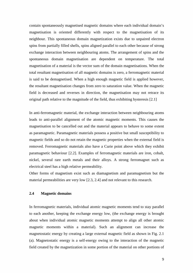
the same material. Therefore within the material, many magnetic domains are created

to lower the external magnetic field as in figures 2.1 (a) and (b). Within each domain,

individual magnetic moments add up to a total domain magnetization [2.2].

Furthermore, the domain magnetizations of neighbouring magnetic domains are

antiparallel. In this configuration, the exchange energy is increased, however the

magnetostatic energy is lowered. Domain walls are formed between magnetic

domains. It should be noted that some of these walls of different orientation occur in

closure domains as illustrated in figure 2.1 (d). The latter are created when the

material divides into magnetic domains to allow more of the magnetic flux to stay

within the material, thereby minimizing magnetostatic energy [2.4].

Fig. 2.1: Rearrangement of domains at the demagnetised state due to the energy

minimization: a) saturated sample with high magnetostatic energy, Em, b) dividing

into two reduces Em c) more division reduces Em further d) free poles eliminated by

closure domains [2.5].

11

2.5 Domain walls

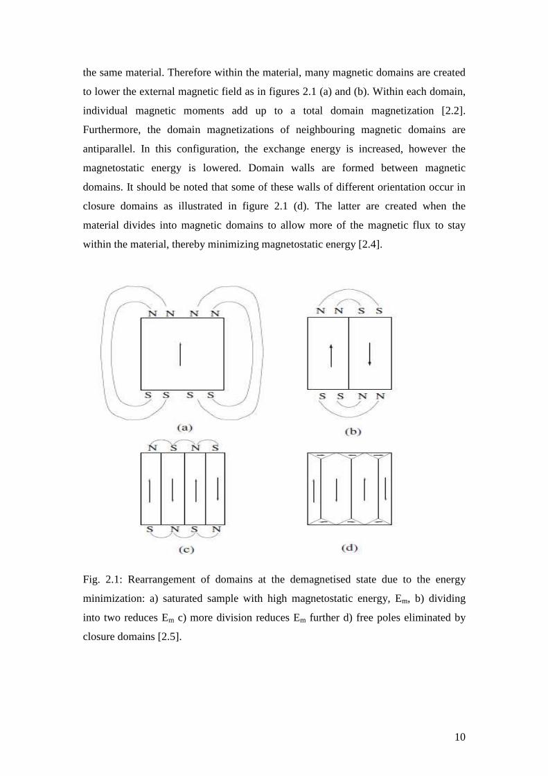
Domains are separated by domain walls containing layers of atoms. As shown in

figure 2.2, within a domain wall, the direction of magnetic moments changes from its

direction in one domain to the direction in another domain leading to the creation of a

transitional region. If the transition from one magnetization direction to another is

abrupt, such as the case for a perfect antiparallel domain magnetization, the exchange

energy will be too high to keep this domain configuration in equilibrium. A domain

wall of a certain thickness that is comprised of atomic magnetic moments of slowly

varying orientation as shown in figure 2.2 ensures a smoother transition opposite to

domain magnetization direction thereby decreasing the exchange energy. The

thickness of the transition layer is determined, being limited by the magnetocrystalline

energy, which tends to keep atomic magnetic moments aligned along one of the easy

directions of the crystal axes in order to maintain a minimum [2.4].

Fig. 2.2: Illustration of domains and domain wall containing atomic magnetic

moments of gradually varying orientation, ensuring a smoother transition to opposite

domain magnetization in a single crystal of iron [2.2].

Since domain magnetizations tend to align with one or more of the preferred

crystallographic axes in iron alloys, domain walls separating domains of different

orientations can be classified as 180° or 90° as in iron depending on the angles these

crystallographic axes make in a specific lattice [2.4].

12

2.6 Magneto crystalline anisotropy energy

Anisotropy is the directional dependence of the properties of a material.

Magnetocrystalline anisotropy is defined as the variation of magnetic properties of a

material from one crystallographic direction to another. For a given magnetic field

along the crystallographic directions, the measured magnetization varies. The concept

of easy and hard directions of magnetization arises because of this. The magnetic field

needed to reach saturation magnetization in the easy direction is less than the field

needed to reach saturation in the hard direction. The easy and hard directions can be

easily determined by measuring the magnetic properties of single crystals magnetised

along different directions and vary from material to material. Iron and electrical steel

alloys have easy direction along <100> and the hard directions along <111> with the

intermediate being <110>.

The amount of magnetocrystalline anisotropy is normally represented in terms of

energy density which varies with crystal structure because of different lattice

symmetries. The grains in electrical steels which have a cubic crystal structure,

magnetocrystalline anisotropy energy, Ek, is given by:

Ek=K1 (α12α2

2+ α22α3

2+ α32 α1

2) + K2 (α12 α2

2 α32) (2.1)

where α1, α2 and α3 are the cosines of the angles between the saturation magnetization,

MS, and the x, y and z axis of the cubic crystal structure. K1 and K2 are the first and

second order cubic anisotropy constants respectively which for 3% silicon iron at

room temperature are 4.8 x 104 J/m3 and 5 x 104 J/m3 respectively [2.2]. A positive

value of K shows a material having the direction of domain moments aligned with the

[100] crystal direction while a negative value show an alignment with the [111]

direction.

2.7 Magnetostatic energy

The magnetostatic energy indicates the total free pole energy of the domain structure.

When considering a piece of ferromagnetic material containing only a single domain,

free magnetic poles exist at the discontinuous ends of the sample. This would create a

13

field within the sample known as the demagnetising field. The demagnetising field

has an energy Em associated with it given by [2.6]:

Em = 1/2 ND M2 (2.2)

where ND is its demagnetising factor of the material. Subdividing the material into

two oppositely magnetised domains will reduce the demagnetising field and hence the

magnetostatic energy. The subdivision would continue indefinitely with each

subsequent division reducing the magnetostatic energy further if the magnetostatic

energy were the only contributing factor.

2.8 Magnetoelastic energy

Application of stress causes reorientation of the atomic magnetic moments of the

lattice. This reorientation takes place because the mechanical strain that is set up in

the lattice moves the magnetic moments away from the easy axis of the lattice. The

magnetic energy that is associated with these lattice strains is called magnetoelastic

energy. Stress has similar effects on both magnetoelastic energy and

magnetocrystalline anisotropy where there is the creation of easy axes of

magnetisation. The magnitude of the magnetoelastic energy, λE , for a cubic crystal

under uniform stress )(σ can be expressed as shown in equation 2.3:

)(3)(2

3131332322121111

23

23

22

22

21

21100 γγααγγααγγαασλγαγαγασλλ ++−++−=E

(2.3)

where 100λ and 111λ are the magnetostriction constants with strains measured under

magnetic field along the <100> and <111> directions respectively. 1γ , 2γ , and 3γ are

the direction cosines of the stress components with respect to the crystal axes [2.7].

2.9 The effect of an externally applied field

If a small magnetic field is applied to a magnetic material such as electrical steel,

magnetisation occurs by the motion of 180° and 90° domain walls until the net force

on all walls is zero. This takes place by the motion of domain walls through the

14

material such that domains in the direction of the applied field grow at the expense of

all others. A second effect that may also occur during magnetisation is that the

magnetic moments within a domain may be rotated out of the easy axes of

magnetisation and into the direction of the applied field. A higher applied magnetic

field than domain wall motion is needed in this effect since the domain magnetisation

is being moved away from the easy axes and is associated with an increase in the

stored magnetocrystalline anisotropy energy [2.8]. The energy due to an externally

applied field can be described by equation 2.4 [2.1] as follows:

φcosHMEH = (2.4)

where H is the applied magnetic field, M is the magnetisation and φ is the angle

between the easy lattice direction and the field.

2.10 Energy loss due to magnetisation

Magnetic materials are characterised uniquely by their B-H loops.

Work is done in changing the magnetisation of a magnetic material resulting in the

dissipation of energy (mainly heat) from the material to its surroundings. As the

material is taken through a magnetisation cycle the time lag between the instantaneous

applied H and the corresponding B of the material results in a typical B-H loop as

shown in figure 2.3.

15

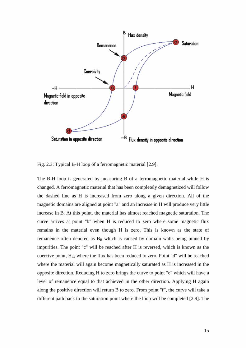
Fig. 2.3: Typical B-H loop of a ferromagnetic material [2.9].

The B-H loop is generated by measuring B of a ferromagnetic material while H is

changed. A ferromagnetic material that has been completely demagnetized will follow

the dashed line as H is increased from zero along a given direction. All of the

magnetic domains are aligned at point "a" and an increase in H will produce very little

increase in B. At this point, the material has almost reached magnetic saturation. The

curve arrives at point "b" when H is reduced to zero where some magnetic flux

remains in the material even though H is zero. This is known as the state of

remanence often denoted as BR which is caused by domain walls being pinned by

impurities. The point "c" will be reached after H is reversed, which is known as the

coercive point, HC, where the flux has been reduced to zero. Point "d" will be reached

where the material will again become magnetically saturated as H is increased in the

opposite direction. Reducing H to zero brings the curve to point "e" which will have a

level of remanence equal to that achieved in the other direction. Applying H again

along the positive direction will return B to zero. From point "f”, the curve will take a

different path back to the saturation point where the loop will be completed [2.9]. The

16

area enclosed by the loop is directly proportional to the energy loss in the material per

unit volume per magnetisation cycle which is often referred to as hysteresis loss.

A number of basic magnetic properties of a material can be determined from the

hysteresis loop viz:

Remanence – This is the magnetic flux density that remains in a material when the

magnetic field is zero. It is the value of B at point b in figure 2.3 and can be

represented with the symbol BR.

Coercivity – This is the amount of reverse magnetic field that is applied to a magnetic

material to make the magnetic flux density to return to zero. It is the value of H at

point c in figure 2.3. It is also known as the coercive field and is symbolised as HC.

Permeability –The ease at which magnetic flux is established in a material defines

the permeability of that material. Permeability (µ) is used to define the relationship

between B and H as:

→→

= HB µ (2.5)

The relationship between B and H in free space is written as:

→→

= HB 0µ (2.6)

B is expressed relative to free space in other mediums as:

→→

= HB r 0µµ (2.7)

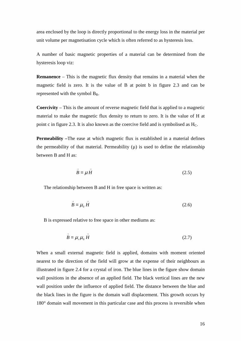
When a small external magnetic field is applied, domains with moment oriented

nearest to the direction of the field will grow at the expense of their neighbours as

illustrated in figure 2.4 for a crystal of iron. The blue lines in the figure show domain

wall positions in the absence of an applied field. The black vertical lines are the new

wall position under the influence of applied field. The distance between the blue and

the black lines in the figure is the domain wall displacement. This growth occurs by

180° domain wall movement in this particular case and this process is reversible when

17

the magnetic field is removed. At higher field amplitude the domain wall motion

becomes irreversible and irreversible domain rotation also occur. When the field

amplitude is further increased, saturation occurs and the sample will be converted into

a single domain. This is the state of technical saturation magnetisation.

Fig.2.4: Schematic diagram showing domains with moments aligned most closely

with the applied field will increase in volume at the expense of the other domains.

2.11 Hysteresis process and energy loss

The wider the B-H loop, the more energy is stored and dissipated in the material.

Permanent magnets which are hard magnetic materials require wider B-H loops to

store more energy while B-H loops of soft magnetic materials like electrical steel

should be narrow to achieve low loss. The anhysteretic (i.e. without hysteresis) B-H

characteristic is ideal for soft magnetic material. Under ac magnetisation, the B-H

loop in figure 2.3 is wider due to additional magnetic fields from the eddy current

(electric currents which are created when the material experiences changes in

magnetic field) and excess losses (explained in section 2.13) and the energy loss per

cycle is higher than under quasi-static (so slowly as appear to be static) condition.

New wall position as a result of applied field

18

These losses are frequency dependent and are referred to as dynamic losses [2.10].

The static hysteresis losses are frequency independent.

The loop area is equal to the total energy lost per cycle for sinusoidal magnetisation.

This total loss can be broken into components which can be expressed as:

Total loss = Static hysteresis Loss + Classical eddy current loss + Excess (anomalous)

loss (2.8)

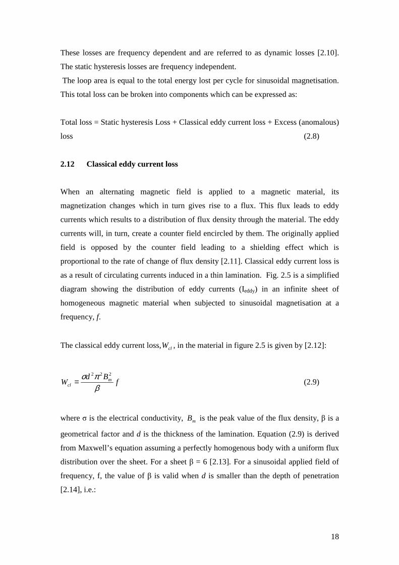
2.12 Classical eddy current loss

When an alternating magnetic field is applied to a magnetic material, its

magnetization changes which in turn gives rise to a flux. This flux leads to eddy

currents which results to a distribution of flux density through the material. The eddy

currents will, in turn, create a counter field encircled by them. The originally applied

field is opposed by the counter field leading to a shielding effect which is

proportional to the rate of change of flux density [2.11]. Classical eddy current loss is

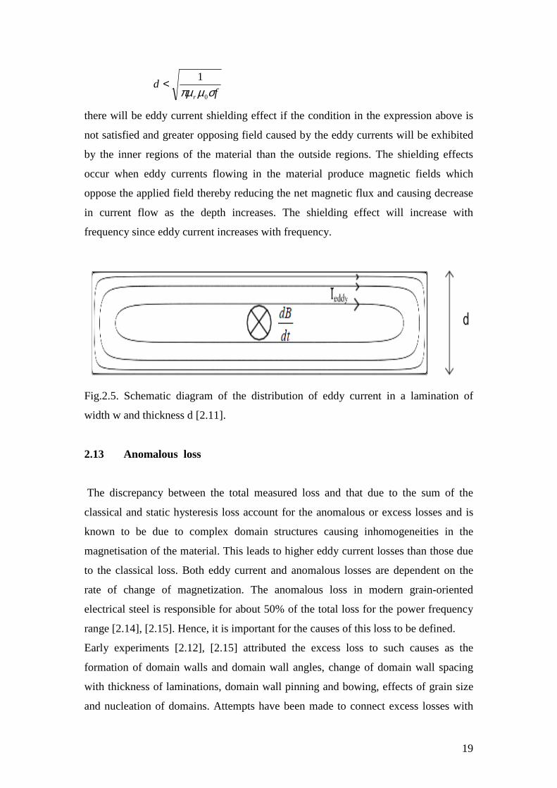
as a result of circulating currents induced in a thin lamination. Fig. 2.5 is a simplified

diagram showing the distribution of eddy currents (Ieddy) in an infinite sheet of

homogeneous magnetic material when subjected to sinusoidal magnetisation at a

frequency, f.

The classical eddy current loss,clW , in the material in figure 2.5 is given by [2.12]:

fBd

W mcl β

πσ 222

= (2.9)

where σ is the electrical conductivity, mB is the peak value of the flux density, β is a

geometrical factor and d is the thickness of the lamination. Equation (2.9) is derived

from Maxwell’s equation assuming a perfectly homogenous body with a uniform flux

distribution over the sheet. For a sheet β = 6 [2.13]. For a sinusoidal applied field of

frequency, f, the value of β is valid when d is smaller than the depth of penetration

[2.14], i.e.:

19

fd

r σµπµ 0

1<

there will be eddy current shielding effect if the condition in the expression above is

not satisfied and greater opposing field caused by the eddy currents will be exhibited

by the inner regions of the material than the outside regions. The shielding effects

occur when eddy currents flowing in the material produce magnetic fields which

oppose the applied field thereby reducing the net magnetic flux and causing decrease

in current flow as the depth increases. The shielding effect will increase with

frequency since eddy current increases with frequency.

Fig.2.5. Schematic diagram of the distribution of eddy current in a lamination of

width w and thickness d [2.11].

2.13 Anomalous loss

The discrepancy between the total measured loss and that due to the sum of the

classical and static hysteresis loss account for the anomalous or excess losses and is

known to be due to complex domain structures causing inhomogeneities in the

magnetisation of the material. This leads to higher eddy current losses than those due

to the classical loss. Both eddy current and anomalous losses are dependent on the

rate of change of magnetization. The anomalous loss in modern grain-oriented

electrical steel is responsible for about 50% of the total loss for the power frequency

range [2.14], [2.15]. Hence, it is important for the causes of this loss to be defined.

Early experiments [2.12], [2.15] attributed the excess loss to such causes as the

formation of domain walls and domain wall angles, change of domain wall spacing

with thickness of laminations, domain wall pinning and bowing, effects of grain size

and nucleation of domains. Attempts have been made to connect excess losses with

20

Barkhausen noise [2.16], or to attribute them to continuous rearrangements of the

domain configuration [2.17]. This loss has been found to occur in many magnetic

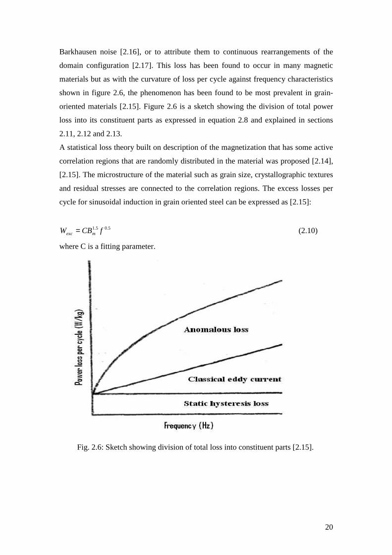
materials but as with the curvature of loss per cycle against frequency characteristics

shown in figure 2.6, the phenomenon has been found to be most prevalent in grain-

oriented materials [2.15]. Figure 2.6 is a sketch showing the division of total power

loss into its constituent parts as expressed in equation 2.8 and explained in sections

2.11, 2.12 and 2.13.

A statistical loss theory built on description of the magnetization that has some active

correlation regions that are randomly distributed in the material was proposed [2.14],

[2.15]. The microstructure of the material such as grain size, crystallographic textures

and residual stresses are connected to the correlation regions. The excess losses per

cycle for sinusoidal induction in grain oriented steel can be expressed as [2.15]:

5.05.1 fCBW mexc = (2.10)

where C is a fitting parameter.

Fig. 2.6: Sketch showing division of total loss into constituent parts [2.15].

21


[2.1] R. M. Bozorth, Ferromagnetism, IEEE Press, New York, 1993.

[2.2] D.C Jiles, Introduction to Magnetism and Magnetic Materials, Chapman and


[2.3] S. Chikazumi, Physics of Magnetism, Oxford University Press Inc, New York,

1997.

[2.4] B.D. Cullity, Introduction to Magnetic Materials, 2nd edition, Addison-Wesley,

New York, 1972.

[2.5] V. Yardley, Magnetic detection of microstructural change in power plant steels,

PhD thesis, University of Cambridge, April 2003.

[2.6] J. W. Shilling and G.L.Jr. House, Magnetic properties and domain structure in

grain-oriented 3% Si-Fe, IEEE Transactions on Magnetics, Vol. 10, No. 2, pp.195-

222,1974.

[2.7] R. Becker, W. Doring, Ferromagnetismus, Springer, Berlin, 1939.

[2.8] P. Anderson, A novel method of measurement and characterisation of

magnetostriction in electrical steels, PhD thesis, Cardiff University, 2000.

[2.9]http://www.ndt.ed.org/EducationResources/CommunityCollege/Mag

Particle/Physics/HysteresisLoop.htm. Accessed on 20th June 2011.

[2.10] S. E. Zirka, Y. I. Moroz, P. Marketos, and A. J. Moses, Evolution of the loss

components in ferromagnetic laminations with induction level and frequency, Journal

of Magnetism and Magnetic Materials, Vol. 320, No. 20, pp.1039–1043, 2008.

[2.11] D. Ribbenfjärd, Electromagnetic transformer modelling including the

ferromagnetic core, Doctoral thesis in Electrical Systems Stockholm, Sweden 2010.

[2.12] G. Bertotti, Hysteresis in Magnetism, Academic Press, Inc., California, USA,

1998.

[2.13] D.C. Jiles, Modelling the effects of eddy current losses on frequency dependent

hysteresis in electrically conducting media, IEEE Transactions on Magnetics, Vol. 30,

No. 6, pp. 4326-4328, 1994.

[2.14] G. Bertotti, General properties of power losses in soft ferromagnetic materials,

IEEE Transactions on Magnetics, Vol. 24, No. 1, pp.621-630, 1988.

[2.15] K.J. Overshott, The use of domain observation in understanding and improving

the magnetic properties of transformer steels, IEEE Transactions on Magnetics, Vol.

12, No. 6, pp.840-845, 1976.

22

[2.16] P. Mazzetti, Block walls correlation and magnetic loss in ferromagnetics, IEEE

Transactions on Magnetics, Vol.14, No. 5, pp.758-763, 1978.

[2.17] J. E. L. Bishop, Enhanced eddy current loss due to domain displacement,

Journal of Magnetism and Magnetic Materials Vol. 49, Issue 3, pp. 241-249, 1985.

23

Chapter 3 Electrical steel production and

processing

3.1 Introduction

Electrical steels may have originated from the work of Barret, Hadfield and Brown in

the turn of the 20th century. They discovered [3.1] that alloying high purity steel with

silicon greatly increased the resistivity of the steel thereby reducing eddy current

losses. Alloying with silicon also improved the magnetic properties by reducing

coercivity and increasing permeability. Another major breakthrough took place in

1934 [3.2] when a rolling process was developed which caused a large proportion of

individual grains in the electrical steel to be aligned with a <001> direction along the

rolling direction of the sheet. In 1940, Armco Steel Corporation developed this

method which was subsequently adopted by other producers of electrical steel from

1953. This preferred orientation is known as the Goss texture and the sheet becomes a

(110) plane.

Grain oriented electrical steel (GOES) has usually a silicon level of 3% by mass. It is

produced in such a way that the best magnetic performance occurs when magnetised

along the rolling direction, due to preferential secondary recrystallisation of [001]

(110) grains. Secondary recrystallisation is a process by which grain size increases

consisting in an exaggerated growth of only a few larger grains at the expense of the

many smaller ones and occur in the presence of conditions which can inhibit normal

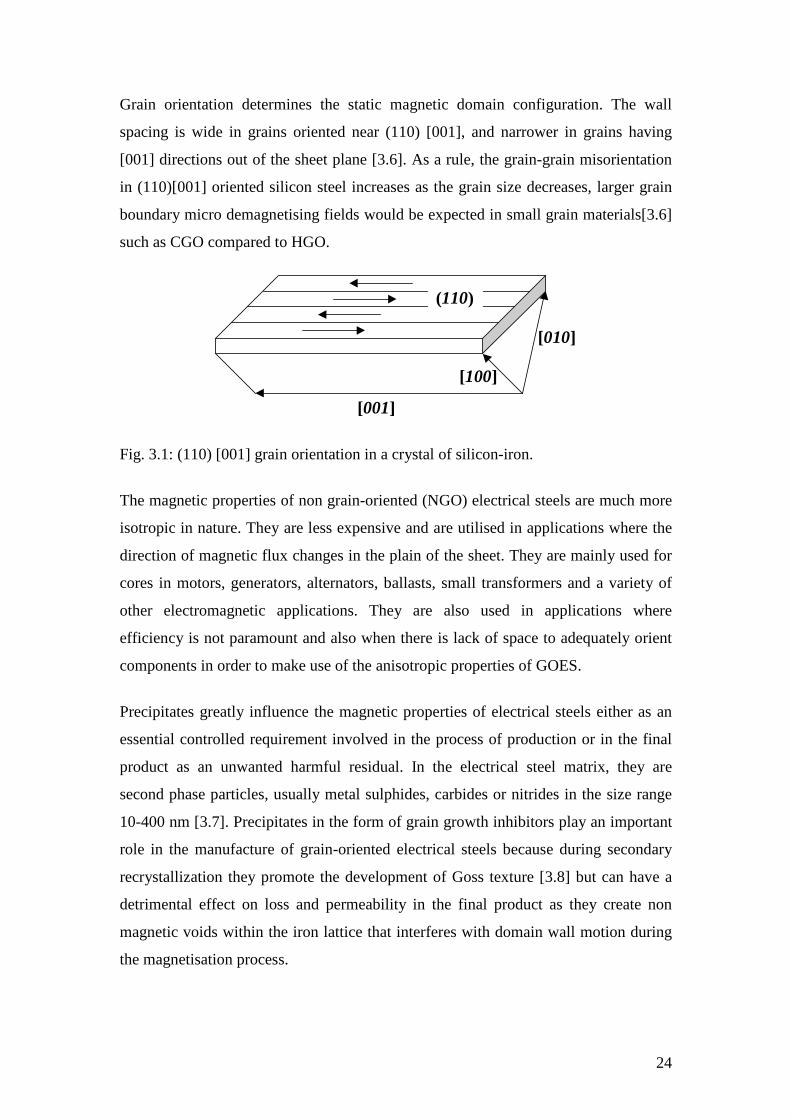
grain growth [3.3]. Figure 3.1 shows the schematic diagram of the [001] (110) grain

orientation in a crystal of silicon iron.

The resulting product had grain-grain misorientation in the angle of yaw of around 7°

and is known as Conventional Grain Oriented (CGO) steel. Nippon Steel Company

exploited this method in 1966 which lead to the development of high permeability

grain oriented silicon steel known as ‘Hi-B’ [3.4] which has grain-grain

misorientation of around 3° [3.5]. In this thesis high permeability grain oriented

silicon steel is referred to as High grain oriented (HGO) steel. The grain size of HGO

is on average higher, approximately 9.0 mm diameter compared to 4.0 mm in CGO.

24

Grain orientation determines the static magnetic domain configuration. The wall

spacing is wide in grains oriented near (110) [001], and narrower in grains having

[001] directions out of the sheet plane [3.6]. As a rule, the grain-grain misorientation

in (110)[001] oriented silicon steel increases as the grain size decreases, larger grain

boundary micro demagnetising fields would be expected in small grain materials[3.6]

such as CGO compared to HGO.

Fig. 3.1: (110) [001] grain orientation in a crystal of silicon-iron.

The magnetic properties of non grain-oriented (NGO) electrical steels are much more

isotropic in nature. They are less expensive and are utilised in applications where the

direction of magnetic flux changes in the plain of the sheet. They are mainly used for

cores in motors, generators, alternators, ballasts, small transformers and a variety of

other electromagnetic applications. They are also used in applications where

efficiency is not paramount and also when there is lack of space to adequately orient

components in order to make use of the anisotropic properties of GOES.

Precipitates greatly influence the magnetic properties of electrical steels either as an

essential controlled requirement involved in the process of production or in the final

product as an unwanted harmful residual. In the electrical steel matrix, they are

second phase particles, usually metal sulphides, carbides or nitrides in the size range

10-400 nm [3.7]. Precipitates in the form of grain growth inhibitors play an important

role in the manufacture of grain-oriented electrical steels because during secondary

recrystallization they promote the development of Goss texture [3.8] but can have a

detrimental effect on loss and permeability in the final product as they create non

magnetic voids within the iron lattice that interferes with domain wall motion during

the magnetisation process.

(110)

[001]

[100]

[010]

25

3.2 Manufacture of grain oriented electrical Steel

3.2.1 Conventional grain oriented electrical steel production route

The steel is produced using the basic oxygen steel (BOS) making process with

elements like carbon, manganese, sulphur and silicon added during the vacuum

degassing stage. Carbon is essential for maintaining the correct phases after hot band

and intermediate anneal and also for the cultivation of the desired texture during cold

reduction [3.9]. Manganese on the other hand with the combination of sulphur forms

manganese sulphide (MnS) during the high temperature coil annealing (HTCA)

process to inhibit primary grain growth. Silicon increases the resistivity of the steel

thereby minimizing eddy currents in the steel laminations. A typical composition of

the added elements could be 0.035% for Carbon, 0.06 % for manganese, 0.025 % for

sulphur and 3.25 % for silicon.

The alloy is cast into ingots and then passed to a reheating stage where the

temperature of the slab is maintained at about 1400°C. The high temperature at this

stage is necessary for the MnS to form solution and well homogenised throughout the

metal. The steel is then rapidly cooled after hot rolling and coiled at around 600°C to

cause the MnS to precipitate in a finely dispersed form to ensure that the correct

microstructure is developed for the eventual growth of the oriented grains in the

finished product. The thickness after hot rolling is normally 1.9 mm.

As shown in figure 3.2, this hot rolled coil is conveyed to the electrical steel

production line where it is side trimmed, then annealed, descaled and pickled. The

steel is initially annealed continuously at around 950°C, descaled by removing the

iron oxide scale physically using iron shot fired at the strip’s surface by a wheel

abrator and then pickled by cleaning in a hydrofluoric and sulphuric acid mixture

which is followed by a hot dip in an alkaline oil solution all in a bid to refine the

metallurgical structure of the hot rolled coil and make it suitable for cold rolling.

The next stage as shown in figure 3.2 is that of cold reduction. The coil is reduced to

around twice the finished gauge. In order to produce steel of flat shape of appropriate

intermediate gauge, the coil is reduced to an intermediate thickness of around 0.6 mm

determined by the final gauge of the strip. High density of dislocations follows this

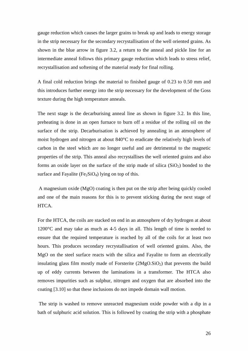
26

gauge reduction which causes the larger grains to break up and leads to energy storage

in the strip necessary for the secondary recrystallisation of the well oriented grains. As

shown in the blue arrow in figure 3.2, a return to the anneal and pickle line for an

intermediate anneal follows this primary gauge reduction which leads to stress relief,

recrystallisation and softening of the material ready for final rolling.

A final cold reduction brings the material to finished gauge of 0.23 to 0.50 mm and

this introduces further energy into the strip necessary for the development of the Goss

texture during the high temperature anneals.

The next stage is the decarburising anneal line as shown in figure 3.2. In this line,

preheating is done in an open furnace to burn off a residue of the rolling oil on the

surface of the strip. Decarburisation is achieved by annealing in an atmosphere of

moist hydrogen and nitrogen at about 840°C to eradicate the relatively high levels of

carbon in the steel which are no longer useful and are detrimental to the magnetic

properties of the strip. This anneal also recrystallises the well oriented grains and also

forms an oxide layer on the surface of the strip made of silica (SiO2) bonded to the

surface and Fayalite (Fe2SiO4) lying on top of this.

A magnesium oxide (MgO) coating is then put on the strip after being quickly cooled

and one of the main reasons for this is to prevent sticking during the next stage of

HTCA.

For the HTCA, the coils are stacked on end in an atmosphere of dry hydrogen at about

1200°C and may take as much as 4-5 days in all. This length of time is needed to

ensure that the required temperature is reached by all of the coils for at least two

hours. This produces secondary recrystallisation of well oriented grains. Also, the

MgO on the steel surface reacts with the silica and Fayalite to form an electrically

insulating glass film mostly made of Forsterite (2MgO.SiO2) that prevents the build

up of eddy currents between the laminations in a transformer. The HTCA also

removes impurities such as sulphur, nitrogen and oxygen that are absorbed into the

coating [3.10] so that these inclusions do not impede domain wall motion.

The strip is washed to remove unreacted magnesium oxide powder with a dip in a

bath of sulphuric acid solution. This is followed by coating the strip with a phosphate

27

solution which is then cured at a temperature of approximately 800°C. The coating

creates a tension at the surface of the steel, due to the effect of the difference in

thermal expansion coefficient between the coating and the steel base during the

application onto the steel surface thereby reducing the power loss and

magnetostriction that occur during magnetisation of the fully processed steel [3.11],

[3.12].

Strip distortions caused by the high temperature coil anneal process are removed by a

thermal flattening process. The strip may also be laser scribed at this stage to improve

magnetic properties.

Finally, the edges of the coil are trimmed before the coil is sent to be packaged or slit

into several widths.

28

Fig.3.2: CGO Electrical Steel Production Process at Cogent Power Ltd, Newport, UK

[3.13].

3.2.2 High permeability grain oriented electrical steel production route

The manufacturing route for HGO differs slightly from that of CGO. HGO utilises

aluminium nitride in addition to MnS as a grain growth inhibitor [3.14] and the cold

reduction is accomplished in one operation. This additional inhibitor is required

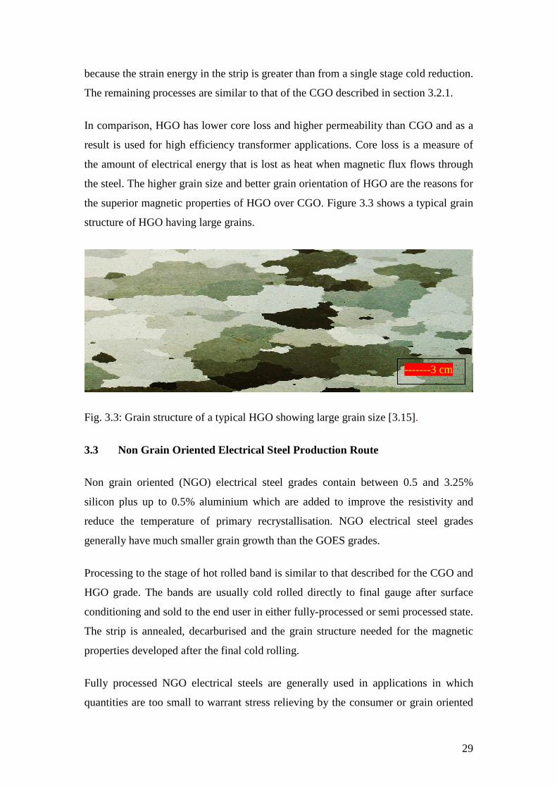
29

because the strain energy in the strip is greater than from a single stage cold reduction.

The remaining processes are similar to that of the CGO described in section 3.2.1.

In comparison, HGO has lower core loss and higher permeability than CGO and as a

result is used for high efficiency transformer applications. Core loss is a measure of

the amount of electrical energy that is lost as heat when magnetic flux flows through

the steel. The higher grain size and better grain orientation of HGO are the reasons for

the superior magnetic properties of HGO over CGO. Figure 3.3 shows a typical grain

structure of HGO having large grains.

Fig. 3.3: Grain structure of a typical HGO showing large grain size [3.15].

3.3 Non Grain Oriented Electrical Steel Production Route

Non grain oriented (NGO) electrical steel grades contain between 0.5 and 3.25%

silicon plus up to 0.5% aluminium which are added to improve the resistivity and

reduce the temperature of primary recrystallisation. NGO electrical steel grades

generally have much smaller grain growth than the GOES grades.

Processing to the stage of hot rolled band is similar to that described for the CGO and

HGO grade. The bands are usually cold rolled directly to final gauge after surface

conditioning and sold to the end user in either fully-processed or semi processed state.

The strip is annealed, decarburised and the grain structure needed for the magnetic

properties developed after the final cold rolling.

Fully processed NGO electrical steels are generally used in applications in which

quantities are too small to warrant stress relieving by the consumer or grain oriented

-------3 cm

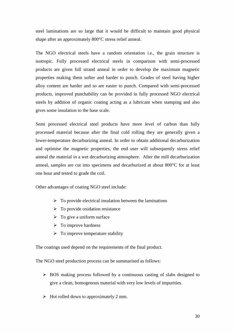
30

steel laminations are so large that it would be difficult to maintain good physical

shape after an approximately 800°C stress relief anneal.

The NGO electrical steels have a random orientation i.e., the grain structure is

isotropic. Fully processed electrical steels in comparison with semi-processed

products are given full strand anneal in order to develop the maximum magnetic

properties making them softer and harder to punch. Grades of steel having higher

alloy content are harder and so are easier to punch. Compared with semi-processed

products, improved punchability can be provided in fully processed NGO electrical

steels by addition of organic coating acting as a lubricant when stamping and also

gives some insulation to the base scale.

Semi processed electrical steel products have more level of carbon than fully

processed material because after the final cold rolling they are generally given a

lower-temperature decarburizing anneal. In order to obtain additional decarburization

and optimise the magnetic properties, the end user will subsequently stress relief

anneal the material in a wet decarburizing atmosphere. After the mill decarburization

anneal, samples are cut into specimens and decarburized at about 800°C for at least

one hour and tested to grade the coil.

Other advantages of coating NGO steel include:

To provide electrical insulation between the laminations

To provide oxidation resistance

To give a uniform surface

To improve hardness

To improve temperature stability

The coatings used depend on the requirements of the final product.

The NGO steel production process can be summarised as follows:

BOS making process followed by a continuous casting of slabs designed to

give a clean, homogenous material with very low levels of impurities.

Hot rolled down to approximately 2 mm.

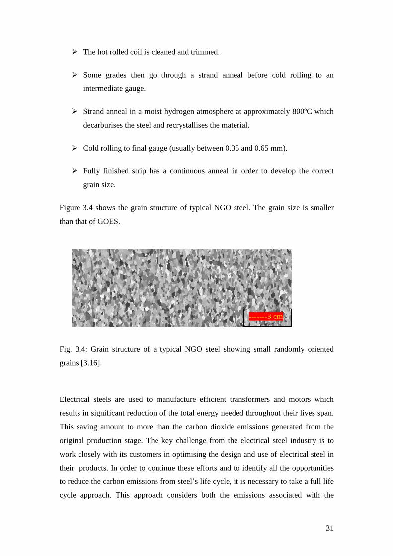
31

The hot rolled coil is cleaned and trimmed.

Some grades then go through a strand anneal before cold rolling to an

intermediate gauge.

Strand anneal in a moist hydrogen atmosphere at approximately 800ºC which

decarburises the steel and recrystallises the material.

Cold rolling to final gauge (usually between 0.35 and 0.65 mm).

Fully finished strip has a continuous anneal in order to develop the correct

grain size.

Figure 3.4 shows the grain structure of typical NGO steel. The grain size is smaller

than that of GOES.

Fig. 3.4: Grain structure of a typical NGO steel showing small randomly oriented

grains [3.16].

Electrical steels are used to manufacture efficient transformers and motors which

results in significant reduction of the total energy needed throughout their lives span.

This saving amount to more than the carbon dioxide emissions generated from the

original production stage. The key challenge from the electrical steel industry is to

work closely with its customers in optimising the design and use of electrical steel in

their products. In order to continue these efforts and to identify all the opportunities

to reduce the carbon emissions from steel’s life cycle, it is necessary to take a full life

cycle approach. This approach considers both the emissions associated with the

-------3 cm

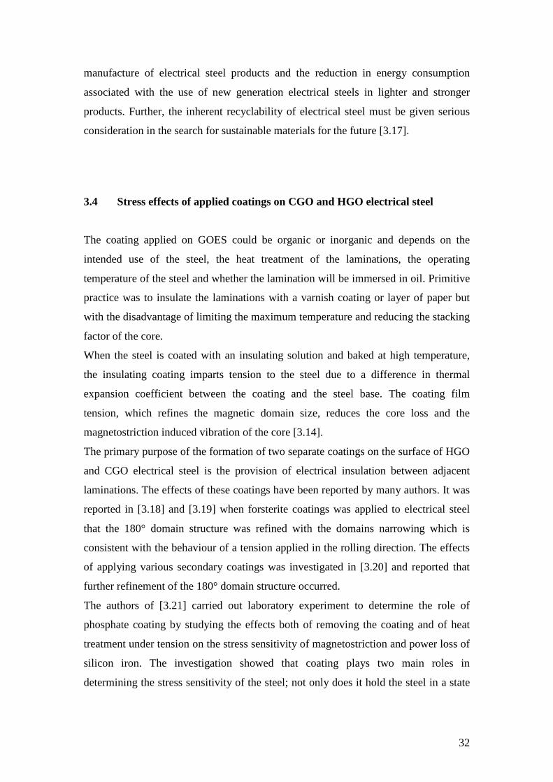
32

manufacture of electrical steel products and the reduction in energy consumption

associated with the use of new generation electrical steels in lighter and stronger

products. Further, the inherent recyclability of electrical steel must be given serious

consideration in the search for sustainable materials for the future [3.17].

3.4 Stress effects of applied coatings on CGO and HGO electrical steel

The coating applied on GOES could be organic or inorganic and depends on the

intended use of the steel, the heat treatment of the laminations, the operating

temperature of the steel and whether the lamination will be immersed in oil. Primitive

practice was to insulate the laminations with a varnish coating or layer of paper but

with the disadvantage of limiting the maximum temperature and reducing the stacking

factor of the core.

When the steel is coated with an insulating solution and baked at high temperature,

the insulating coating imparts tension to the steel due to a difference in thermal

expansion coefficient between the coating and the steel base. The coating film

tension, which refines the magnetic domain size, reduces the core loss and the

magnetostriction induced vibration of the core [3.14].

The primary purpose of the formation of two separate coatings on the surface of HGO

and CGO electrical steel is the provision of electrical insulation between adjacent

laminations. The effects of these coatings have been reported by many authors. It was

reported in [3.18] and [3.19] when forsterite coatings was applied to electrical steel

that the 180° domain structure was refined with the domains narrowing which is

consistent with the behaviour of a tension applied in the rolling direction. The effects

of applying various secondary coatings was investigated in [3.20] and reported that

further refinement of the 180° domain structure occurred.

The authors of [3.21] carried out laboratory experiment to determine the role of

phosphate coating by studying the effects both of removing the coating and of heat

treatment under tension on the stress sensitivity of magnetostriction and power loss of

silicon iron. The investigation showed that coating plays two main roles in

determining the stress sensitivity of the steel; not only does it hold the steel in a state

33

of isotropic tension, caused by the different contractions but it can also hold the steel

in a state of uniaxial tension along the rolling direction.

Nippon Steel conducted research to solve the shortcomings of a conventional

insulating coating composed of magnesium phosphate alone and developed a new

insulating coating of the colloidal silica-aluminium phosphate based acid system

[3.22].

3.4.1 Longitudinal tensile stress

When a tension is applied parallel to the rolling direction in grain oriented electrical

steel, little effect will be produced on a well oriented grain with mainly [001]

domains. However, there will be refinement of domains with transverse

supplementary structure leading to the disappearance of the supplementary structure.

The resultant effect of the application of a tension in the <100> direction is the

increase of the magnetoelastic energy of the transverse domains while at the same

time decreasing that of the longitudinal domains [3.10]. This will make the

longitudinal domains to become energetically more favourable and so will grow at the

expense of the transverse supplementary domains. The magnetostatic energy will

increase because of the removal of the supplementary structure by the applied stress.

This is countered by reducing the demagnetising field by the narrowing of the [001]

domains [3.1]. Fig.3.5a shows domain pattern of grain oriented steel without tension.

Fig.3.5b shows the domain pattern under applied tension of 3 MPa in the rolling

direction with the domains refined. The rolling direction is 180° to the direction of the

bar domains in both figures. The images were obtained using the equipment and

technique described in sections 5.5.2 and 8.2 respectively.

34

(a) (b)

Fig .3.5: Domain structure of grain oriented steel (a) without tension (b) with tension.

3.4.2 Longitudinal compressive stress

When a compressive stress is applied along the rolling direction of grain oriented

electrical steel, the magnetoelastic energy of the [001] domains increases. This leads

to a rearrangement of the domain structure to give two patterns that are distinct viz:

Stress Pattern I and Stress Pattern II, after a transition stage where the domain pattern

seem to disappear completely [3.23]. Stress pattern I is the simplest of the structures

and is the first to appear. The now energetically favourable [100] domains with small

[001] flux closure domains constitutes the bulk of the domain. Increasing the

compressive stress results in further increase of the magnetoelastic energy of the flux

closure domains and consequently decreasing in size at the expense of the [100]

domains. The decreasing size of the closure domains leads to a simultaneous

narrowing of the bulk domains by the same mechanism as with applied tension.

In stress pattern II which is more complex, the main domains are still in the [100]

direction and the domain wall lie in the <010> direction. The main domains no longer

transverse the strip at 90° to the rolling direction. The surface closure structure has a

zigzag pattern although still consisting of [001] domains. It was proposed in [3.19]

that the transition between stress pattern I and stress pattern II occur due to the

decreasing domain width with stress of the main [100] domains of stress pattern I and

the corresponding increase in wall energy. It was also shown in [3.19], how the

domain wall energy of stress pattern II decreases with increasing stress and therefore

becomes more energetically favourable. This transition typically occurs at a

compressive stress of 2 to 3 MPa in a well oriented grain [3.10]. Figure 3.6 shows the

domain structure of unstressed domains, stress pattern I and II in grain oriented steel.

-------2 mm -------2 mm

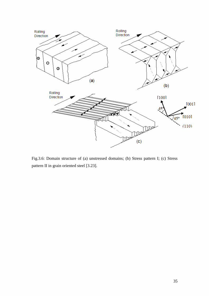
35

Fig.3.6: Domain structure of (a) unstressed domains; (b) Stress pattern I; (c) Stress

pattern II in grain oriented steel [3.23].

36


[3.1] W. F. Barrett, W. Brown and R. A. Hadfield, Researches on different alloys of

iron, Journal of Institute of Electrical Engineers, Vol. 31, pp. 674-722, 1902.

[3.2] N. P. Goss, New development in electrical strip steels characterized by fine

grain structure approaching properties of a single crystal, Transactions of American

Society on Metals, Vol. 23, pp. 515-531, 1935.

[3.3] C. Antonione, G. D. Gatta, G. Riontino and G. Venturello, Grain growth and

secondary recrystallisation in iron, Journal of Material Science, Vol. 8, No. 1, pp. 1-

10, 1973.

[3.4] S. Taguchi, A. Sakakura and H. Takashima, US Patent 3287183, 1966.

[3.5] M. F. Littmann, Structures and magnetic properties of grain oriented 3.2%

silicon-iron, Journal of Applied Physics, Vol. 38, issue 3, pp. 1104-1108, 1967.

[3.6] J. W. Shilling and G.L.Jr. Houze, Magnetic properties and domain structure in

grain-oriented 3% Si-Fe, IEEE Transactions on Magnetics, Vol. 10, No. 2, pp. 195-

222, 1974.

[3.7] K. Jenkins and M. Lindenmo, Precipitates in electrical steel, Journal of

Magnetism and Magnetic Material, Vol. 320, pp. 2423-2429, 2008.

[3.8] S. Turner, A. Moses, J. Hall, and K. Jenkins, The effect of precipitate size on


Physics, Vol. 107, issue 3, pp. 307-309, 2010.

[3.9] A. Coombs, Solid and Laminated Soft Magnetic Materials, UK Magnetics

Society Seminar Paper, 1997.

[3.10] P. Anderson, A novel method of measurement and characterisation of

magnetostriction in electrical steels, PhD thesis, Cardiff University, 2000.

[3.11] S. Cho, S. Kim, J. Soh, and S. Han, Effect of tension coating on iron loss at

frequencies below 1 KHz in thin-gauged 3% Si-Fe sheets, IEEE Transactions on

Magnetics, Vol. 45, no. 10, pp. 4165-4168, 2009.

[3.12] A. J. Moses, H. V. Patel and P. I. Williams, Challenges in quantifying

Barkhausen noise in electrical steel, Electromagnetic NDE(X), Vol. 28, pp. 178-185,

2007.

[3.13] http://www.orb.gb.com/downloads/cogent_brochure.pdf. Accessed on 28th

June 2011.

[3.14] http://en.wikipedia.org/wiki/Electrical_steel. Accessed on 30th June 2011.

37

[3.15]. A. J. Moses, Electrical Steels: Past, Present and Future Developments, IEE

Proceedings, Vol.137, Pt. A, No.5, pp. 233-245, 1990.

[3.16] D. S. Petrovic, Non-oriented electrical steel sheets, Materials and technology,

Vol. 44, issue 6, pp. 317-325, 2010.

[3.17] http://www.worldsteel.org/publications/position-papers/Steel-s-contribution-to-

a-low-carbon-future.html . Accessed 13th April 2012.

[3.18] O. Tanaka, H. Kobayashi and E. Minematsu, New insulating coating for grain

oriented electrical steel, Journal of Material Engineering, Vol.13, pp. 161-168, 1991.

[3.19] S. D. Washko, T. H. Shen and W. G. Morris, The effect of forsterite coatings

on the magnetic properties and domain structure of grain oriented 3% SiFe, Journal of

Applied Physics, Vol. 53, No. 11, pp. 8296-8298,1982.

[3.20] W. G. Morris and J. W. Shilling, Effect of forsterite coatings on the domain

structure of grain oriented 3% SiFe, IEEE Transactions on Magnetics, Vol.14, No.1,

pp. 14-17, 1978.

[3.21] S. D. Washco and E. G. Choby, Evidence for the effectiveness of stress

coatings in improving the magnetic properties of high permeability 3% SiFe, IEEE

Transactions on Magnetics, Vol. 15, No. 6, pp. 1586-1591, 1979.

[3.22] A. J. Moses, S. M. Pegler and J. E, Thompson, Role of phosphate coating in

determining the magnetic properties of Goss Oriented Silicon Iron, Proceedings of the

IEE, vol. 119, No.8, pp. 1222-1228, 1972.

[3.23] L. A. Dijkstra and H. M. Martius, Domain pattern in silicon iron under stress',

Review of Modern Physics, Vol. 25, 146-150, 1953.

.

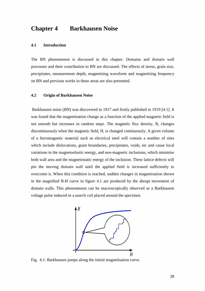
38

Chapter 4 Barkhausen Noise

4.1 Introduction

The BN phenomenon is discussed in this chapter. Domains and domain wall

processes and their contribution to BN are discussed. The effects of stress, grain size,

precipitates, measurement depth, magnetising waveform and magnetising frequency

on BN and previous works in these areas are also presented.

4.2 Origin of Barkhausen Noise

Barkhausen noise (BN) was discovered in 1917 and firstly published in 1919 [4.1]. It

was found that the magnetisation change as a function of the applied magnetic field is

not smooth but increases in random steps. The magnetic flux density, B, changes

discontinuously when the magnetic field, H, is changed continuously. A given volume

of a ferromagnetic material such as electrical steel will contain a number of sites

which include dislocations, grain boundaries, precipitates, voids, etc and cause local

variations in the magnetoelastic energy, and non-magnetic inclusions, which minimise

both wall area and the magnetostatic energy of the inclusion. These lattice defects will

pin the moving domain wall until the applied field is increased sufficiently to

overcome it. When this condition is reached, sudden changes in magnetisation shown

in the magnified B-H curve in figure 4.1 are produced by the abrupt movement of

domain walls. This phenomenon can be macroscopically observed as a Barkhausen

voltage pulse induced in a search coil placed around the specimen.

Fig. 4.1: Barkhausen jumps along the initial magnetisation curve.

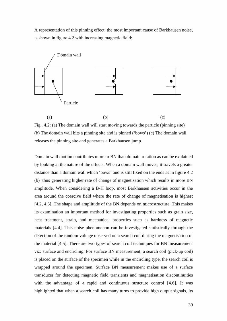
39

A representation of this pinning effect, the most important cause of Barkhausen noise,

is shown in figure 4.2 with increasing magnetic field:

(a) (b) (c)

Fig . 4.2: (a) The domain wall will start moving towards the particle (pinning site)

(b) The domain wall hits a pinning site and is pinned (‘bows’) (c) The domain wall

releases the pinning site and generates a Barkhausen jump.

Domain wall motion contributes more to BN than domain rotation as can be explained

by looking at the nature of the effects. When a domain wall moves, it travels a greater

distance than a domain wall which ‘bows’ and is still fixed on the ends as in figure 4.2

(b) thus generating higher rate of change of magnetisation which results in more BN

amplitude. When considering a B-H loop, most Barkhausen activities occur in the

area around the coercive field where the rate of change of magnetisation is highest

[4.2, 4.3]. The shape and amplitude of the BN depends on microstructure. This makes

its examination an important method for investigating properties such as grain size,

heat treatment, strain, and mechanical properties such as hardness of magnetic

materials [4.4]. This noise phenomenon can be investigated statistically through the

detection of the random voltage observed on a search coil during the magnetisation of

the material [4.5]. There are two types of search coil techniques for BN measurement

viz: surface and encircling. For surface BN measurement, a search coil (pick-up coil)

is placed on the surface of the specimen while in the encircling type, the search coil is

wrapped around the specimen. Surface BN measurement makes use of a surface

transducer for detecting magnetic field transients and magnetisation discontinuities

with the advantage of a rapid and continuous structure control [4.6]. It was

highlighted that when a search coil has many turns to provide high output signals, its

Domain wall

Particle

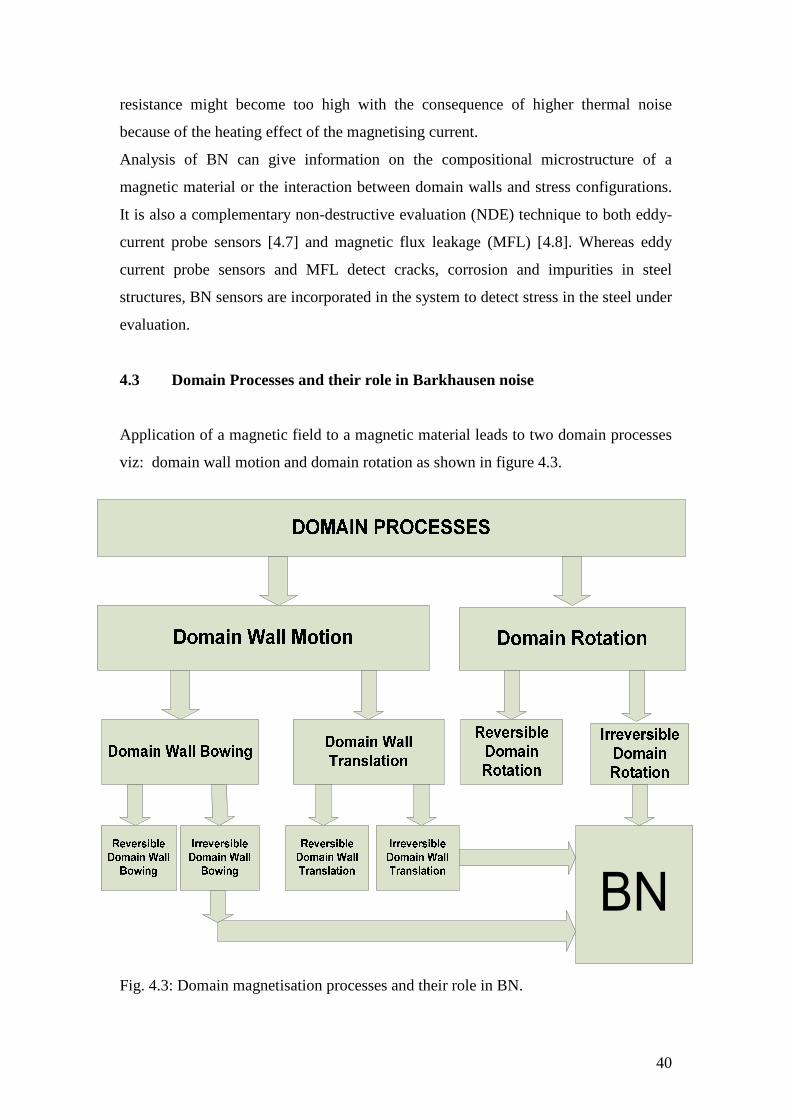
40

resistance might become too high with the consequence of higher thermal noise

because of the heating effect of the magnetising current.

Analysis of BN can give information on the compositional microstructure of a

magnetic material or the interaction between domain walls and stress configurations.

It is also a complementary non-destructive evaluation (NDE) technique to both eddy-

current probe sensors [4.7] and magnetic flux leakage (MFL) [4.8]. Whereas eddy

current probe sensors and MFL detect cracks, corrosion and impurities in steel

structures, BN sensors are incorporated in the system to detect stress in the steel under

evaluation.

4.3 Domain Processes and their role in Barkhausen noise

Application of a magnetic field to a magnetic material leads to two domain processes

viz: domain wall motion and domain rotation as shown in figure 4.3.

Fig. 4.3: Domain magnetisation processes and their role in BN.

41

Three reversible and three irreversible domain processes occur. A reversible process

is one such that if the external magnetic field is reduced or removed the magnetisation

in the material returns to its original value. Domain wall motion is classified into

domain wall bowing and domain rotation. Domain wall bowing can be either

reversible or irreversible under certain conditions. When a low magnetic field is

applied, this process is reversible. The domain wall is likened to a rubber band which

extends under the influence of the magnetic field and returns to its original position

when the magnetic field is removed. When the domain wall is sufficiently deformed

such that the extension continues without further increase of the magnetic field the

effect becomes irreversible. A second even more important process which makes this

effect irreversible is when the domain wall, while extending, encounters a further

pinning site. This pinning site prevents the wall from returning to its original position

when the field is removed. The pinning effect occurs when the magnetic field further

increases and the domain wall breaks away from its pinning sites [4.4].

Domain wall translation is usually irreversible unless no pinning sites exist in the

material. Hence when the field is removed, all walls can return to their original

positions. Irreversible domain wall translation is the effect which contributes most to

BN generation.

Domain rotation is a process where the atomic magnetic moments in a domain are

turned from their original position towards the direction of a magnetic field applied to

the sample. It is reversible in low fields when magnetic moments just slightly turn

from their preferred low energy axis towards the direction of the magnetic field. For

intermediate to high fields domain rotation becomes irreversible when the magnetic

moments change their direction from their original preferred low energy axis to the

one which is closest to the field direction. This occurs when the field energy

overcomes the anisotropy energy [4.5]. All the irreversible domain processes lead to

BN.

4.4 Barkhausen noise and 180° domain walls

It is believed that BN occur mainly because of 180° domain wall motion [4.5], [4.9]

as the 90° domain walls have associated stress fields with them making

magnetisations lie at right angles on either side of the wall, causing lattice spacing to

be slightly larger in the direction of magnetisation. The resulting strain impedes 90°

42

domain wall motion, making it less significant than 180° domain walls that have a

higher velocity [4.10]. In [4.11] and [4.12], the authors developed a method of

determining the size distribution and number of Barkhausen jumps over all or any part

of the magnetisation cycle. A slowly varying magnetic field was applied to a

specimen hard-drawn iron and the Barkhausen jumps were amplified and detected as

voltage pulses on an oscilloscope for visual inspection. Based on the above

experimental investigation the authors concluded that Barkhausen jumps originate

mostly from movement of 180º domain walls [4.13]. They observed that the number

of countable Barkhausen discontinuities in a half-cycle was very large and to

minimise overlap effects the rate of change of magnetic field must be vey small.

4.5 Barkhausen noise and stress effects

Due to its high sensitivity to stress, BN can be used in NDE of elastic and plastic

deformations [4.14]. A stress will change the bulk magnetization of a ferromagnetic

material even if no field is applied [4.5]. Magnetic domains undergo stress-induced

volume changes just as they do under the influence of an external magnetic field. The

magnetic field needed to move a domain wall across a pinning site and the wall

energy gradient increases as the internal elastic stress increase [4.4]. The pinning sites

themselves are also influenced by stress. In fact, elastic strain effects are more

influential on BN than plastic strain effects [4.15]. To gain a better idea of how stress

influences BN, its influence on magnetic domains should be considered.

An applied stress disturbs the balance of the energy terms described in chapter 2. If no

external field is present, the magnetostatic energy is zero and the magnetocrystalline

and magnetoelastic energy are dominant [4.16]. Both magnetocrystalline and

magnetoelastic energy compete to determine the direction of the domain

magnetization under stress. A new energy configuration is achieved when under

applied uniaxial tensile stress domains lying closest to the stress direction grow at the

expense of domains with perpendicular domain magnetization while the domains with

magnetic moments perpendicular to the axis of applied stress become favourable

energetically under compressive stress [4.17].

43

Generally under stress, the 180° domain wall population in the stress direction

increases if the stress is tensile. Since BN is associated with wall pinning, a lower

signal is obtained with compressive stress, and a higher for tensile stress [4.18].

The influence of applied stress on BN amplitude was first observed in [4.9]. It was

shown that the most favourably oriented domains increased in size primarily by

movement of 180° walls when the applied field was increased. A magnetising

frequency of 0.09 Hz was used to magnetise the samples. In [4.19], Barkhausen

discontinuities were generated by a triangular waveform with a maximum frequency

of 4 Hz.

BN was generated by a 50 Hz applied magnetic field in [4.20]. It was found that an ac

excitation field to generate Barkhausen jumps gives a cleaner and more reproducible

Barkhausen signal. BN was also found to increase with frequency. This same trend

was found at both high and low fields in this thesis.

Investigation of the BN envelope amplitude and its relation to surface stress in a

surface modified steel specimen was conducted in [4.21]. The result showed that the

Barkhausen signal envelope amplitude decreases with increasing compressive stress.

4.6 Barkhausen noise and depth variation in electrical steel

BN is sensitive to changes in the surface condition of electrical steel because the

magnetic properties are closely linked to stress through magnetoelastic coupling and

are reported to be within the frequency range of 20-200 kHz in steel in [4.22]. The

frequency bandwidth of the detected signal can be selected to control the depth

sensitivity to analyse material condition at different depths. Changes in material

condition at different depths inside the material are evaluated by the selective

attenuation of high frequency components of the BN signal as a result of eddy

currents.

The authors in [4.21] found the frequency band at which BN was detected to be

inversely proportional to skin depth using the standard skin depth expression given in

section 2.12. These frequencies correspond to the mean of each of the five frequency

bands over which measurements were taken. The values of the classical skin depth for

a material with σ = 1 x 106 Ω-l.m-l and µr = 200 are given for different frequencies in

Table 4.1.

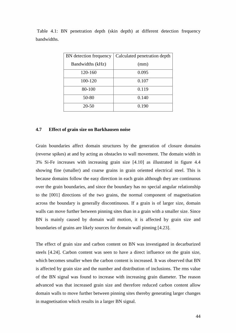
44

Table 4.1: BN penetration depth (skin depth) at different detection frequency

bandwidths.

4.7 Effect of grain size on Barkhausen noise

Grain boundaries affect domain structures by the generation of closure domains

(reverse spikes) at and by acting as obstacles to wall movement. The domain width in

3% Si-Fe increases with increasing grain size [4.10] as illustrated in figure 4.4

showing fine (smaller) and coarse grains in grain oriented electrical steel. This is

because domains follow the easy direction in each grain although they are continuous

over the grain boundaries, and since the boundary has no special angular relationship

to the [001] directions of the two grains, the normal component of magnetisation

across the boundary is generally discontinuous. If a grain is of larger size, domain

walls can move further between pinning sites than in a grain with a smaller size. Since

BN is mainly caused by domain wall motion, it is affected by grain size and

boundaries of grains are likely sources for domain wall pinning [4.23].

The effect of grain size and carbon content on BN was investigated in decarburized

steels [4.24]. Carbon content was seen to have a direct influence on the grain size,

which becomes smaller when the carbon content is increased. It was observed that BN

is affected by grain size and the number and distribution of inclusions. The rms value

of the BN signal was found to increase with increasing grain diameter. The reason

advanced was that increased grain size and therefore reduced carbon content allow

domain walls to move further between pinning sites thereby generating larger changes

in magnetisation which results in a larger BN signal.

BN detection frequency

Bandwidths (kHz)

Calculated penetration depth

(mm)

120-160 0.095

100-120 0.107

80-100 0.119

50-80 0.140

20-50 0.190

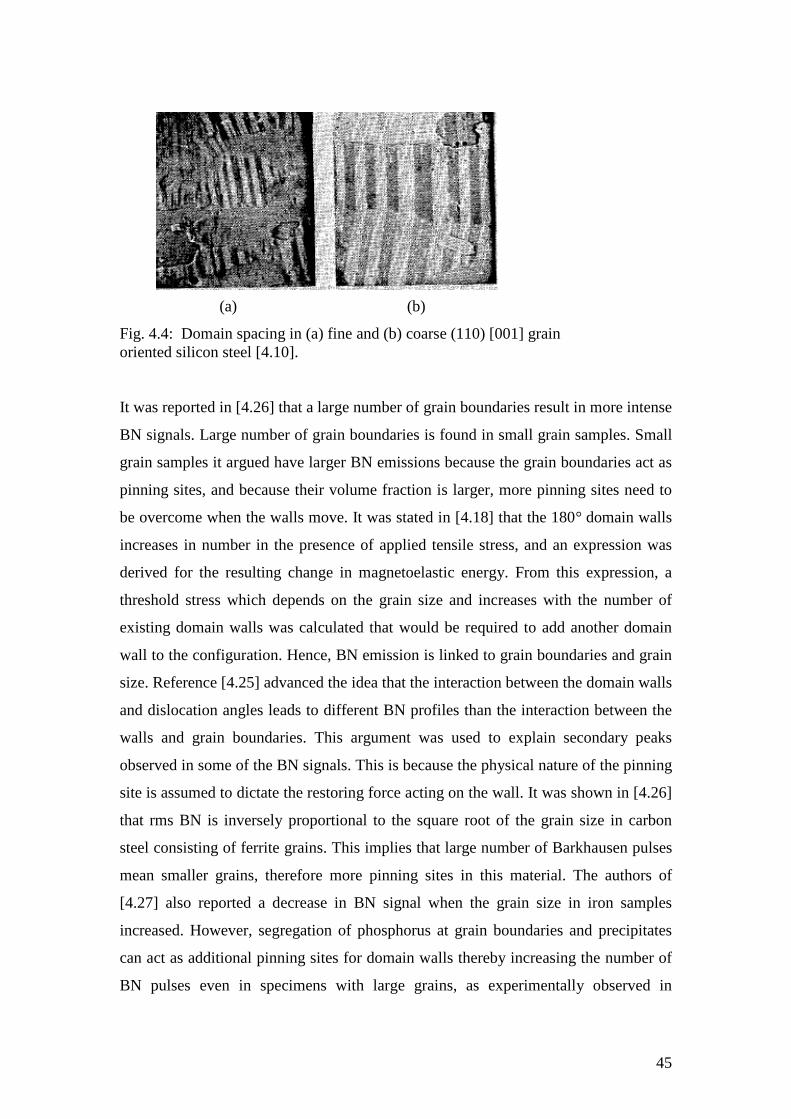
45

(a) (b)

Fig. 4.4: Domain spacing in (a) fine and (b) coarse (110) [001] grain oriented silicon steel [4.10].

It was reported in [4.26] that a large number of grain boundaries result in more intense

BN signals. Large number of grain boundaries is found in small grain samples. Small

grain samples it argued have larger BN emissions because the grain boundaries act as

pinning sites, and because their volume fraction is larger, more pinning sites need to

be overcome when the walls move. It was stated in [4.18] that the 180° domain walls

increases in number in the presence of applied tensile stress, and an expression was

derived for the resulting change in magnetoelastic energy. From this expression, a

threshold stress which depends on the grain size and increases with the number of

existing domain walls was calculated that would be required to add another domain

wall to the configuration. Hence, BN emission is linked to grain boundaries and grain

size. Reference [4.25] advanced the idea that the interaction between the domain walls

and dislocation angles leads to different BN profiles than the interaction between the

walls and grain boundaries. This argument was used to explain secondary peaks

observed in some of the BN signals. This is because the physical nature of the pinning

site is assumed to dictate the restoring force acting on the wall. It was shown in [4.26]

that rms BN is inversely proportional to the square root of the grain size in carbon

steel consisting of ferrite grains. This implies that large number of Barkhausen pulses

mean smaller grains, therefore more pinning sites in this material. The authors of

[4.27] also reported a decrease in BN signal when the grain size in iron samples

increased. However, segregation of phosphorus at grain boundaries and precipitates

can act as additional pinning sites for domain walls thereby increasing the number of

BN pulses even in specimens with large grains, as experimentally observed in

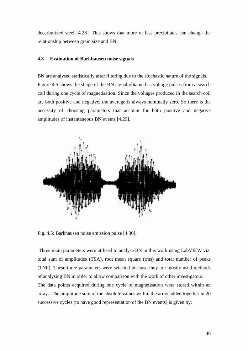
46

decarburized steel [4.28]. This shows that more or less precipitates can change the

relationship between grain size and BN.

4.8 Evaluation of Barkhausen noise signals

BN are analysed statistically after filtering due to the stochastic nature of the signals.

Figure 4.5 shows the shape of the BN signal obtained as voltage pulses from a search

coil during one cycle of magnetisation. Since the voltages produced in the search coil

are both positive and negative, the average is always nominally zero. So there is the

necessity of choosing parameters that account for both positive and negative

amplitudes of instantaneous BN events [4.29].

Fig. 4.5: Barkhausen noise emission pulse [4.30].

Three main parameters were utilised to analyse BN in this work using LabVIEW viz:

total sum of amplitudes (TSA), root mean square (rms) and total number of peaks

(TNP). These three parameters were selected because they are mostly used methods

of analysing BN in order to allow comparison with the work of other investigators.

The data points acquired during one cycle of magnetisation were stored within an

array. The amplitude sum of the absolute values within the array added together in 20

successive cycles (to have good representation of the BN events) is given by:

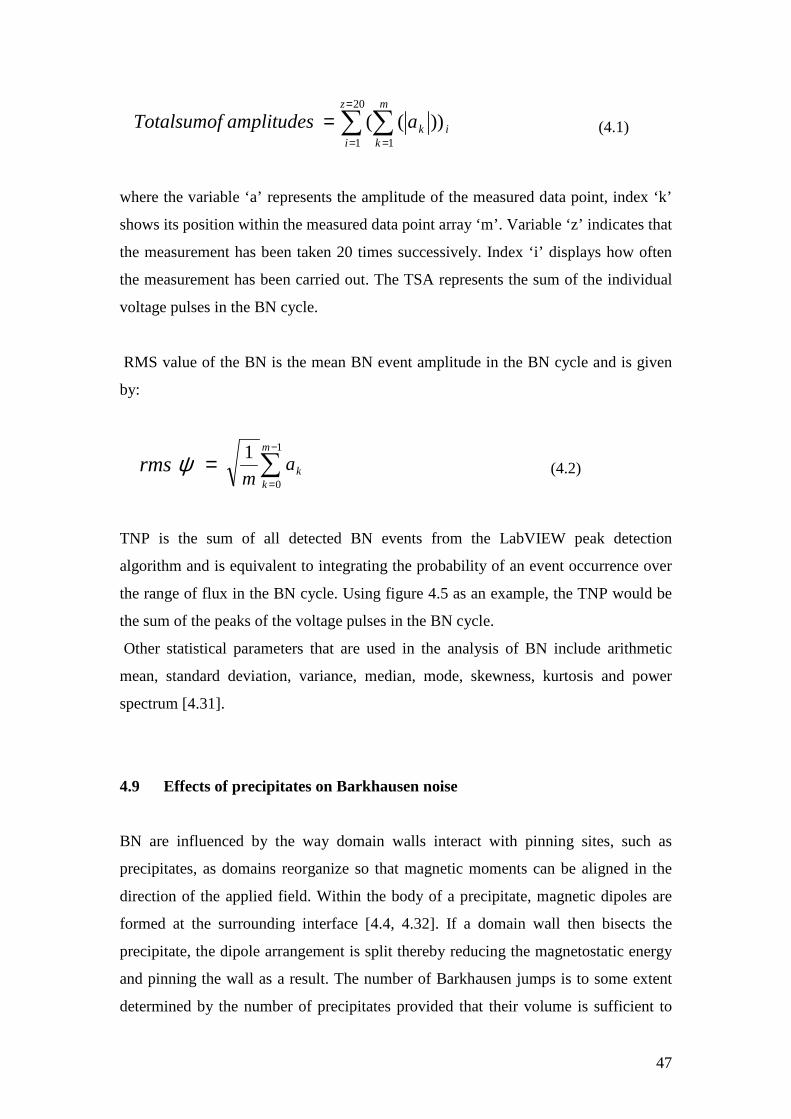
47

∑ ∑=

= =

=20

1 1

))((z

i

m

kikaamplitudesTotalsumof (4.1)

where the variable ‘a’ represents the amplitude of the measured data point, index ‘k’

shows its position within the measured data point array ‘m’. Variable ‘z’ indicates that

the measurement has been taken 20 times successively. Index ‘i’ displays how often

the measurement has been carried out. The TSA represents the sum of the individual

voltage pulses in the BN cycle.

RMS value of the BN is the mean BN event amplitude in the BN cycle and is given

by:

=ψrms ∑−

=

1

0

1 m

kka

m (4.2)

TNP is the sum of all detected BN events from the LabVIEW peak detection

algorithm and is equivalent to integrating the probability of an event occurrence over

the range of flux in the BN cycle. Using figure 4.5 as an example, the TNP would be

the sum of the peaks of the voltage pulses in the BN cycle.

Other statistical parameters that are used in the analysis of BN include arithmetic

mean, standard deviation, variance, median, mode, skewness, kurtosis and power

spectrum [4.31].

4.9 Effects of precipitates on Barkhausen noise

BN are influenced by the way domain walls interact with pinning sites, such as

precipitates, as domains reorganize so that magnetic moments can be aligned in the

direction of the applied field. Within the body of a precipitate, magnetic dipoles are

formed at the surrounding interface [4.4, 4.32]. If a domain wall then bisects the

precipitate, the dipole arrangement is split thereby reducing the magnetostatic energy

and pinning the wall as a result. The number of Barkhausen jumps is to some extent

determined by the number of precipitates provided that their volume is sufficient to

48

cause pinning. This makes BN an important tool for evaluating the scale of interaction

between precipitates of different sizes and magnetic domains.

The presence of copper-manganese sulphide (CuMnS) precipitates increased the rms

BN in grain oriented steel but precipitates which are relatively small compared to the

width of domain walls, approximately 150 nm, for 180° domain wall do not impede

domain wall motion [4.33]. This is because the inclusions are completely engulfed by

the wall, and thus the dipole surrounding the inclusion is maintained.

4.10 Effects of magnetising waveform on Barkhausen noise

The influence of sinusoidal, triangular and square wave form excitation on

Barkhausen emissions were investigated in [4.34]. The frequency spectra of

sinusoidal and triangular alternating field excitations showed similar behaviours but

the spectrum under square wave excitation was different due to the existence of high

frequency components during square wave switching. It was observed that changes in

the field waveform led to different emission pulse shapes. When a square wave

excitation was used the total sum of amplitude of the Barkhausen pulse was four times

higher than in the case of a triangle excitation. Under sinusoidal excitation, the total

sum of total sum of amplitude of the Barkhausen pulse was about 1.6 times higher

than under triangle excitation. It was also found that the signal to noise ratio changed,

square wave excitation had the highest signal to noise ratio and lowest for triangle

excitation. Nevertheless, sinusoidal and triangle waveform excitation were rated to be

more suitable than square wave excitation because the latter can lead to spurious

signals (harmonics) because of the high frequency content at the voltage step.

4.11 Effects of magnetising frequency on Barkhausen noise

The influence of magnetising frequency and ac flux density on BN per cycle of

pipeline steel magnetised up to 50 Hz, 1.5 T was detected by a surface mounted coil

[4.35]. Increasing the flux density caused the Barkhausen noise to initially increase

then decrease at high flux density. It was also shown that the BN increases with

increasing magnetising frequency.

49

The research in [4.31] showed both an increase of Barkhausen noise with increasing

flux density and increasing magnetising frequency for electrical steel. When the BN

amplitude was plotted against magnetising frequency while the peak flux density was

held constant, a linear relationship between BN amplitude and frequency was found.

A benefit of a higher frequency of magnetisation is that the time needed to capture a

cycle is reduced. For BN measurement at quasi-static dc, the period of the

magnetising waveform will be a few seconds or more while at a frequency of 50 Hz,

the capturing time is reduced to 20 ms if events in one cycle are captured.

50


[4.1] H. Barkhausen, Gerausche bien ummagnetisieren von eisen, Physikalishe

Zeitschr, 20, pp. 401-403, 1919.

[4.2] H. V. Patel, S. Zurek, T. Meydan, D.C Jiles, and L. Li, A new adaptive

automated feedback system for Barkhausen signal measurement, Sensors and

Actuators, Vol. 129, pp. 112-117, 2006.

[4.3] D. C. Jiles, The effect of stress on magnetic Barkhausen activity in

ferromagnetic steels, IEEE Transactions on Magnetics, Vol. 25, No.5 , pp. 3455-3457,

1989.

[4.4] D. C. Jiles, Introduction to Magnetism and magnetic materials, Chapman and


[4.5] S. Chikazumi, Physics of Magnetism, Oxford University Press Inc, New York,

1997.

[4.6] S. Saynajakangas, A new surface transducer for generating and detecting

magnetic field transients in ferromagnetics, IEEE Transactions on Magnetics, Vol. 10,

No.1, pp. 44-50, 1974.

[4.7] S. Nath, B. Wincheski, J. P Fulton and M. Namkung, Study of the new eddy

current non-destructive testing sensor on ferromagnetic materials, IEEE Transactions

on Magnetics, Vol. 30, No.6, pp. 4644-4646, 1994.

[4.8] V. Babber, B. Shiari and L. Clapham, Mechanical damage detection with

magnetic flux leakage tools: modelling the effect of localized residual stresses, IEEE

Transactions on Magnetics, Vol. 40, No.1, pp. 43-49, 2004.

[4.9] C. G. Gardner, G. A. Matzkanin and D. L. Davidson, The influence of

mechanical stress on magnetization processes and Barkhausen jumps in ferromagnetic

materials, International Journal of Nondestructive Testing, Vol. 3, No. 2, pp. 131-

169, 1971.


grain-oriented 3% Si-Fe, IEEE Transactions on Magnetics, Vol. 10, No. 2, pp. 195-

222, 1974.

[4.11] H. D. Bush and R. S. Tebble, The Barkhausen effect, Proceedings of the

Physical Society London, Vol. 60, No. 4, pp. 370-381, 1948.

[4.12] R. Tebble, S. Skidmore and L. Corner, The Barkhausen effect, Proc. Phys. Soc.

London, A63, pp. 739-761, 1950.

51

[4.13] E. Stoner, The analysis of magnetic curves, Reviews of Modern Physics,

Vol.25, No.1, pp. 2-16, 1953.

[4.14] C. G. Stefanita, Surface magnetic Barkhausen noise response to plastic yield

of steel, Ph.D. Thesis, Department of Physics, Queen’s University, Kingston, Ontario,

Canada, 1999.

[4.15] C. G. Stefanita, D.L. Atherton and L. Clapham, Plastic versus elastic

deformation effects on magnetic Barkhausen noise in steel, Acta Materialia, 48, pp.

3545-3551, 2000.

[4.16] B. D. Cullity, Introduction to Magnetic Materials, 2nd edition, Addison-

Wesley, New York, 1972.

[4.17] D. Utrata and M. Namkung, Uniaxial stress effects on the low-field

magnetoacoustic interactions in low and medium carbon steels, Review of Progress in

Quantitative Non destructive Evaluation, Vol. 2, pp. 1585-1592, 1987.

[4.18] T. W. Krause, L. Clapham, A. Pattantyus and D.L. Atherton, Investigation of

the stress dependent magnetic easy axis in steel using magnetic Barkhausen noise ,

Journal of Applied Physics, Vol. 79, No.8, pp. 4242-4252, 1996.

[4.19] S. Titto, On the influence of microstructure on magnetisation transitions,

Applied Physics Series No. 119, UDC 621.317.49:620.18, pp. 1-77, 1977.

[4.20] L. B. Sipahi, D. C. Jiles and D. Chandler; Comprehensive analysis of

Barkhausen emission spectra using pulse height analysis, frequency spectrum, and

pulse wave form analysis, Journal of Applied Physics, Vol. 73, No.10, pp. 5623-

5625, 1993.

[4.21] D. C. Jiles, and L. Suominen, Effects of surface stress on computer simulation

of Barkhausen effect emissions: model predictions and comparison with X-ray

diffraction studies, IEEE Transactions on Magnetics, Vol. 30, No. 6, pp. 4924-4926,

1994.

[4.22] A. P. Parakka, J. Batey, and D. C. Jiles, Effect of surface mechanical changes

on magnetic Barkhausen emissions, IEEE Transactions on Magnetics, Vol. 33, No 5,

pp. 4026-4028, 1997.

[4.23] G. Bertotti, F. Fiorillo and A. Montorsi, The role of grain size in the

magnetization process of soft magnetic materials, Journal of Applied Physics, Vol.

67, issue 9, pp. 5574-5576, 1990.

52

[4.24] R. Ranjan, D. C. Jiles and P. K. Rastogi, Magnetic Properties of Decarburized

steels: An investigation of the effects of grain size and carbon content, IEEE

Transactions on Magnetics, Vol. 23, No. 3, pp. 1869-1876, 1987.

[4.25] D. H. L. Ng, K. S. Cho, M. L. Wong, S. L. I. Chan, X-Y. Ma, and C. C. H. Lo,

Study of microstructure, mechanical properties, and magnetization process in low

carbon steel bars by Barkhausen emission, Material Science and Engineering A, Vol.

358, pp.186-198, 2003.

[4.26] H. Sakamoto, M. Okada, and M. Homma, Theoretical analysis of Barkhausen

noise in carbon steels, IEEE Transactions on Magnetics, Vol. 23, No.5, pp. 2236-

2238, 1987.

[4.27] C. Gatelier-Rothea, J. Chicois, R. Fougeres and P. Fleischmann,

Characterization of pure iron (130 P.P.M.) and carbon-iron binary alloy by

Barkhausen noise measurements: Study of the influence of stress and microstructure,

Acta Materialia , Vol. 46, pp. 4873-4882, 1998.

[4.28] R. Ranjan, D.C. Jiles, O. Buck, R.B. Thompson, Grain size measurement using

magnetic and acoustic Barkhausen noise, Journal of Applied Physics, Vol. 61, issue 8,

pp. 3199-3202, 1987.

[4.29] V. E. Iordache, E. Hug, and N. Buiron, Magnetic behaviour versus tensile

deformation mechanisms in a non-oriented Fe- (3 wt %) Si steel, Material Science and

Engineering, A359, pp. 62-74, 2003.

[4.30] M. Willcox and T. Mysak, An introduction to Barkhausen noise and its

applications, Insight NDT, pp. 1-19, 2004.

[4.31] K. Hartmann, Relationships between Barkhausen noise, power loss and

Magnetostriction in Grain-oriented silicon iron, PhD thesis, Cardiff University,

March 2003.

[4.32] L. J. Dijkstra and C. Wert, Effect of inclusion on the coercive force of iron,

Physical Review, Vol. 79, pp. 979-985, 1950.

[4.33] S. Turner, A. Moses, J. Hall, and K. Jenkins, The effect of precipitate size on


Physics, Vol. 107, issue 3, pp. 307-309, 2010.

[4.34] L. B Sipahi, D.C. Jiles, and D. Chandler, Comprehensive analysis of

Barkhausen emission spectra using pulse height analysis, frequency spectrum, and

pulse wave form analysis, Journal of Applied Physics Vol. 73, issue 10, pp. 5623-

5625, 1993.

53

[4.35] A. Dhar and D. L. Atherton, Influence of magnetizing parameters on the

magnetic Barkhausen noise, IEEE Transactions on Magnetics, Vol. 28, No.6, pp.

3363-3366, 1992.

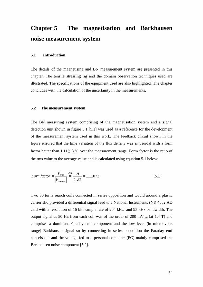
54

Chapter 5 The magnetisation and Barkhausen

noise measurement system

5.1 Introduction

The details of the magnetising and BN measurement system are presented in this

chapter. The tensile stressing rig and the domain observation techniques used are

illustrated. The specifications of the equipment used are also highlighted. The chapter

concludes with the calculation of the uncertainty in the measurements.

5.2 The measurement system

The BN measuring system comprising of the magnetisation system and a signal

detection unit shown in figure 5.1 [5.1] was used as a reference for the development

of the measurement system used in this work. The feedback circuit shown in the

figure ensured that the time variation of the flux density was sinusoidal with a form

factor better than 1.11+− 3 % over the measurement range. Form factor is the ratio of

the rms value to the average value and is calculated using equation 5.1 below:

11072.12.2

=== πideal

average

rms

V

VFormfactor (5.1)

Two 80 turns search coils connected in series opposition and would around a plastic

carrier slid provided a differential signal feed to a National Instruments (NI) 4552 AD

card with a resolution of 16 bit, sample rate of 204 kHz and 95 kHz bandwidth. The

output signal at 50 Hz from each coil was of the order of 200 mVrms (at 1.4 T) and

comprises a dominant Faraday emf component and the low level (in micro volts

range) Barkhausen signal so by connecting in series opposition the Faraday emf

cancels out and the voltage fed to a personal computer (PC) mainly comprised the

Barkhausen noise component [5.2].

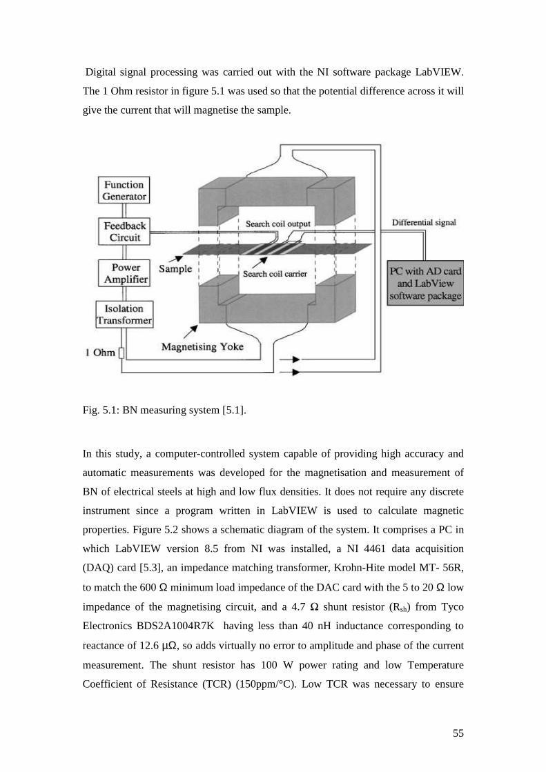
55

Digital signal processing was carried out with the NI software package LabVIEW.

The 1 Ohm resistor in figure 5.1 was used so that the potential difference across it will

give the current that will magnetise the sample.

Fig. 5.1: BN measuring system [5.1].

In this study, a computer-controlled system capable of providing high accuracy and

automatic measurements was developed for the magnetisation and measurement of

BN of electrical steels at high and low flux densities. It does not require any discrete

instrument since a program written in LabVIEW is used to calculate magnetic

properties. Figure 5.2 shows a schematic diagram of the system. It comprises a PC in

which LabVIEW version 8.5 from NI was installed, a NI 4461 data acquisition

(DAQ) card [5.3], an impedance matching transformer, Krohn-Hite model MT- 56R,

to match the 600 Ω minimum load impedance of the DAC card with the 5 to 20 Ω low

impedance of the magnetising circuit, and a 4.7 Ω shunt resistor (Rsh) from Tyco

Electronics BDS2A1004R7K having less than 40 nH inductance corresponding to

reactance of 12.6 µΩ, so adds virtually no error to amplitude and phase of the current

measurement. The shunt resistor has 100 W power rating and low Temperature

Coefficient of Resistance (TCR) (150ppm/°C). Low TCR was necessary to ensure

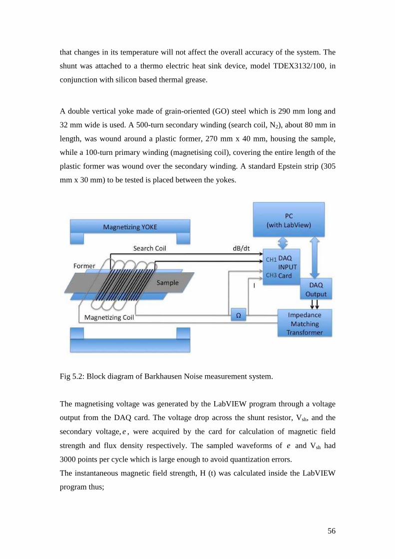
56

that changes in its temperature will not affect the overall accuracy of the system. The

shunt was attached to a thermo electric heat sink device, model TDEX3132/100, in

conjunction with silicon based thermal grease.

A double vertical yoke made of grain-oriented (GO) steel which is 290 mm long and

32 mm wide is used. A 500-turn secondary winding (search coil, N2), about 80 mm in

length, was wound around a plastic former, 270 mm x 40 mm, housing the sample,

while a 100-turn primary winding (magnetising coil), covering the entire length of the

plastic former was wound over the secondary winding. A standard Epstein strip (305

mm x 30 mm) to be tested is placed between the yokes.

Fig 5.2: Block diagram of Barkhausen Noise measurement system.

The magnetising voltage was generated by the LabVIEW program through a voltage

output from the DAQ card. The voltage drop across the shunt resistor, Vsh, and the

secondary voltage,e, were acquired by the card for calculation of magnetic field

strength and flux density respectively. The sampled waveforms of e and Vsh had

3000 points per cycle which is large enough to avoid quantization errors.

The instantaneous magnetic field strength, H (t) was calculated inside the LabVIEW

program thus;

57

ml

tiNtH

)()( 1= (5.2)

wheresh

sh

R

Vti =)( , 1N is the number of primary turns, ml is the magnetic path length,

which is the distance between the inner edges of the yoke which is 0.27 m in this

system.

The instantaneous flux density B (t) was obtained by means of digital integration of

the e signal as:

edtmN

ltB ∫−=

2

)(ρ

(5.3)

where l is the sample length, m is the mass of the sample, and ρ is the density of the

sample.

The specific power loss,P , was determined by multiplying the total energy, W , by

the magnetising frequency, f , over ρ . The amount of energy lost when magnetising

a magnetic material is related to the B-H loop area. The total energy needed if a

material is taken through a complete B-H loop is given by:

dBHW .∫= 3/ mJ (5.4)

Therefore the specific power loss is:

dtdt

dBH

fP ).(.∫=

ρ kgW / (5.5)

The AC relative permeability,rµ , was derived from:

peak

peakr H

B

0µµ = (5.6)

58

where peakH is the peak value of magnetic field andpeakB is the peak flux density.

peakB and peakH were determined numerically by using the maximum function in

LabVIEW.

A feedback control system implemented in LabVIEW was used to control the flux

density and to make the induced secondary voltage waveforms sinusoidal to have

repeatable and comparable measurements. The form factor (FF) of the induced

secondary voltage was maintained at 1.111+− 0.3% which satisfies the recommendation

in [5.4] to ensure that the time variation of the flux density was sinusoidal over the

measurement range. Figure 5.3 shows the procedure for each measurement. Firstly, a

table of Bpeak values and the measurement criteria which are the 0.3% error of Bpeak

and the 0.3% error of the ideal FF of the induced secondary voltage is read. This is

followed by applying the first magnetising waveform to the single sheet tester. If the

criteria are met, the flux density and the magnetic field waveforms are averaged to

minimise random errors and improve repeatability [5.5], otherwise the magnetising

waveform is adjusted by the feedback algorithm. After averaging, the criteria are re-

checked then the measurement data for this point is saved. A spread sheet file is

generated if all the values of Bpeak are measured and the sample is demagnetised by

reducing the magnetic field gradually to zero.

The system is also capable of low-field measurements because the 24 bit resolution of

the NI data acquisition card makes it capable of sensing signals as small as 10-6 V.

The system shown in figure 5.2 was used to measure power loss, permeability,

coercivity, magnetic field and B-H loops.

59

Fig. 5.3: Flowchart showing procedure of each measurement of the single strip tester

[5.6].

Magnetising

Read eand Vsh

Meet the criteria?

Averaging

Re-check the criteria

Last value of Bpeak

Save data

Go to next Bpeak

Generate a spread sheet file

Demagnetising

End

Adjusting magnetising

voltage

Start

Read Bpeak table & criteria

Yes

Yes

Yes

No

No

No

60

5.3 Measurement and evaluation of Barkhausen noise signals

The secondary voltage was filtered to remove the dominant Faraday emf in order to

obtain the BN signals. A digital band pass filter was used so that components in the

range 25 kHz to 75 kHz were detected at a magnetizing frequency of 50 Hz. It was at

this bandwidth that the Barkhausen emission which is maximum at the coercive points

was detected. As observed previously in section 4.6 from the work of others, BN

detection frequency lie any where in the range of 20 kHz – 200 kHz.

One search coil technique rather than a double coil arrangement is used to avoid

losing some Barkhausen events in the subtraction process [5.7]. Using two search

coils connected in series opposition has been mentioned in section 5.2. This is the

differential search coil arrangement with the advantage of eliminating the dominant

Faraday emf component which allows for the selection of the smallest input range and

the best resolution of the data acquisition card. The disadvantage of the differential

coil arrangement is that some Barkhausen jumps cancel each other [5.2, 5.7].

The major challenge in BN measurement is the reduction of background noise. It was

also reported in [5.1] that one way to improve background noise measurements with a

single search coil would be to use an acquisition system with a high resolution. The

low noise NI4461 card with 24 bit resolution and a sampling rate of 204.8 KHz and

92 KHz bandwidth was chosen to take the measurements to minimize the influence of

thermal noise. The card was placed in a PXI (Peripheral component interconnect

eXtension for Instrumentation) platform instead of in a computer system hence it

operates in a predictable environment which means the measurements are more

reliable and repeatable. In order to reduce environmental noise, the yokes, sample and

search coil carrier were placed in a noise shielding chamber. Figure 5.4 shows the

measurement system in the noise shielding chamber and the DAQ in a PXI interface.

The computer monitor was remote from the measuring system to avoid interference

with the measurements. Coaxial cables were used for all connection leads. The noise

level of the measurement system is more than 100 times lower than the lowest BN

signal to be measured as shown in figure 6.10.

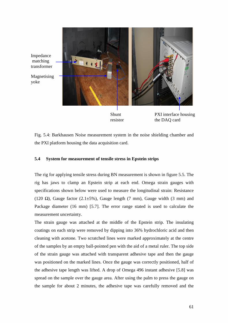
61

Fig. 5.4: Barkhausen Noise measurement system in the noise shielding chamber and

the PXI platform housing the data acquisition card.

5.4 System for measurement of tensile stress in Epstein strips

The rig for applying tensile stress during BN measurement is shown in figure 5.5. The

rig has jaws to clamp an Epstein strip at each end. Omega strain gauges with

specifications shown below were used to measure the longitudinal strain: Resistance

(120 Ω), Gauge factor (2.1±5%), Gauge length (7 mm), Gauge width (3 mm) and

Package diameter (16 mm) [5.7]. The error range stated is used to calculate the

measurement uncertainty.

The strain gauge was attached at the middle of the Epstein strip. The insulating

coatings on each strip were removed by dipping into 36% hydrochloric acid and then

cleaning with acetone. Two scratched lines were marked approximately at the centre

of the samples by an empty ball-pointed pen with the aid of a metal ruler. The top side

of the strain gauge was attached with transparent adhesive tape and then the gauge

was positioned on the marked lines. Once the gauge was correctly positioned, half of

the adhesive tape length was lifted. A drop of Omega 496 instant adhesive [5.8] was

spread on the sample over the gauge area. After using the palm to press the gauge on

the sample for about 2 minutes, the adhesive tape was carefully removed and the

Impedance matching transformer

Magnetising yoke

Shunt resistor

PXI interface housing the DAQ card

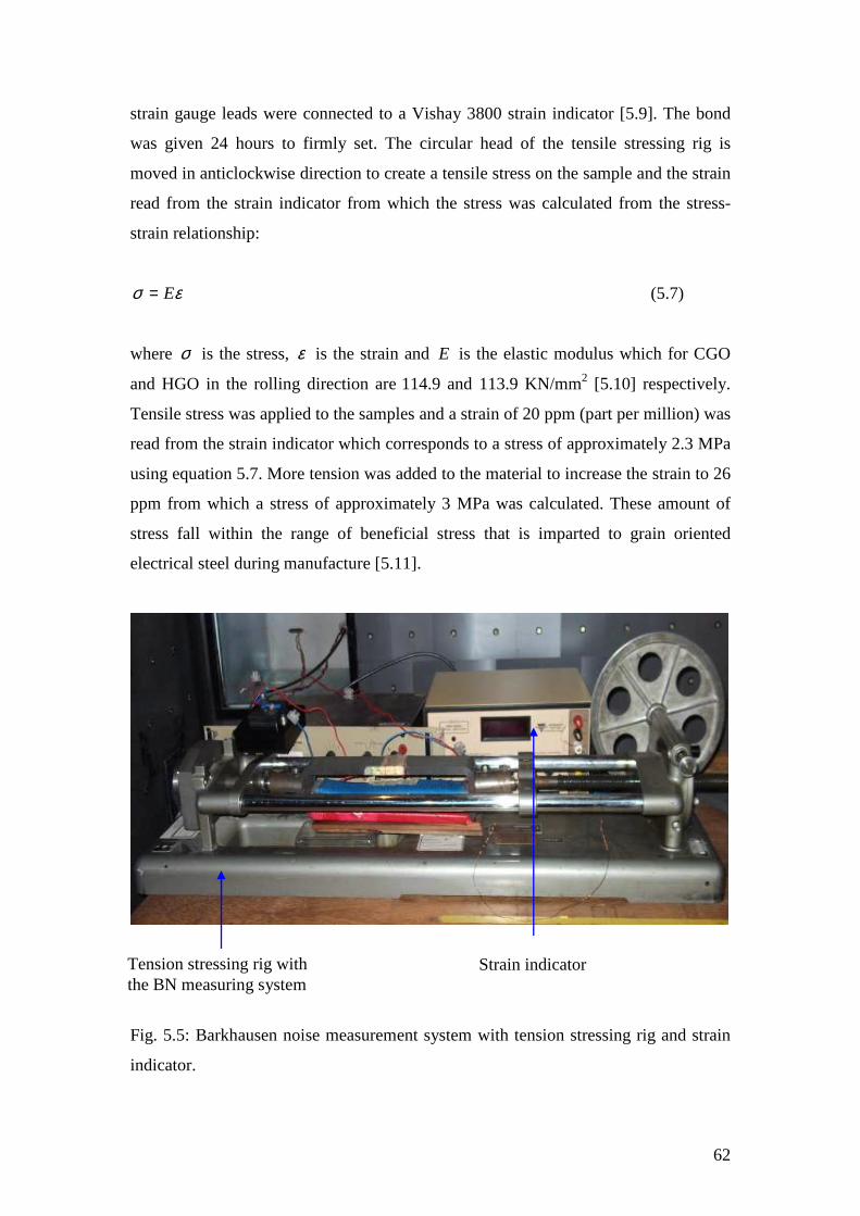
62

strain gauge leads were connected to a Vishay 3800 strain indicator [5.9]. The bond

was given 24 hours to firmly set. The circular head of the tensile stressing rig is

moved in anticlockwise direction to create a tensile stress on the sample and the strain

read from the strain indicator from which the stress was calculated from the stress-

strain relationship:

εσ E= (5.7)

where σ is the stress, ε is the strain and E is the elastic modulus which for CGO

and HGO in the rolling direction are 114.9 and 113.9 KN/mm2 [5.10] respectively.

Tensile stress was applied to the samples and a strain of 20 ppm (part per million) was

read from the strain indicator which corresponds to a stress of approximately 2.3 MPa

using equation 5.7. More tension was added to the material to increase the strain to 26

ppm from which a stress of approximately 3 MPa was calculated. These amount of

stress fall within the range of beneficial stress that is imparted to grain oriented

electrical steel during manufacture [5.11].

Fig. 5.5: Barkhausen noise measurement system with tension stressing rig and strain

indicator.

Tension stressing rig with the BN measuring system

Strain indicator

63

5.5 Methods used for domain observation

Magnetic domains are observed and studied so as to understand the properties of

magnetic materials. Domains are regions of uniform magnetisation which are so

arranged for energy minimization in the material. There are a number of different

methods used to study the domain structure of magnetic materials. The magnetic

domain viewer and the Kerr magneto-optic (KMO) effect [5.12] are the methods used

in this work to observe the domains in the coated and decoated samples respectively.

The KMO technique makes use of the longitudinal Kerr effect to form domain

patterns [5.13].

5.5.1 The magnetic domain viewer

In this method, a magnetic pattern is formed in the magnetic domain viewer. The

domain viewer uses colloidal magnetic particles to detect surface leakage fields. By

applying a low vertical dc magnetic field using an enwrapping coil, the small

ferromagnetic particles congregate on the domains that are in the direction of the

magnetic field and avoid the others that are not in the field’s direction. This makes for

the observed domain contrast in the sample under observation. The domain patterns of

coated CGO and HGO steels observed in this work using the domain viewer are

shown in figures 8.1a and 8.2a respectively.

5.5.2 The Kerr magneto-optic technique

The principle of operation of the KMO effect is that the light reflected from the

surface of the specimen to be observed will interact with the magnetization at the

specimen surface. This interaction will rotate the polarisation plane of the light and

the difference between the incident and reflected beams can be utilized to study the

magnetisation within different regions of the specimen.

The magnetic domain structure of the prepared samples was examined using a low-

magnification longitudinal Kerr effect microscope. The schematic diagram of the

components of a Kerr microscope is shown in figure 5.6. A high pressure mercury

light that illuminates the sample is the light source which is reflected with changes in

polarization, amplitude, and phase determined by the orientation of the magnetisation.

This light is reflected back through the sample under observation through the

64

polarizing beam splitter and the analyzer before being focused on the camera after

under going changes due to the orientation of the magnetization. The second polarizer

(analyser) functions as a filter for the light which reflects off the sample without

changes in polarization. The rotation angle of the polarization is very low and

consequently the signal of the Kerr-affected light is very weak. This weak signal

passes through the analyzer into the camera which is connected to a computer for

image processing and enhancement [5.14]. Three types of Kerr effect microscopy are

used viz: polar, transverse and longitudinal. The polar case have the magnetization

normal to the reflecting surface while in the transverse case, the magnetization vector

in the surface is normal to the plane of incidence. In the longitudinal case, the

magnetization vector is in the plane of incidence and parallel to the surface. It is used

widely in electrical steel due to comparably better contrast than other Kerr effects.

The KMO technique was preferred to other domain imaging techniques in this

research because it is ideal for view relatively large domains with high image contrast.

The CGO and HGO electrical steel used in this research have relatively large

domains. The high image contrast obtainable often eliminates the need for image

processing. The second reason for choosing KMO technique is that no optical

elements other than the sample exist between the polariser and the analyser, there is

no depolarisation of the light beam.

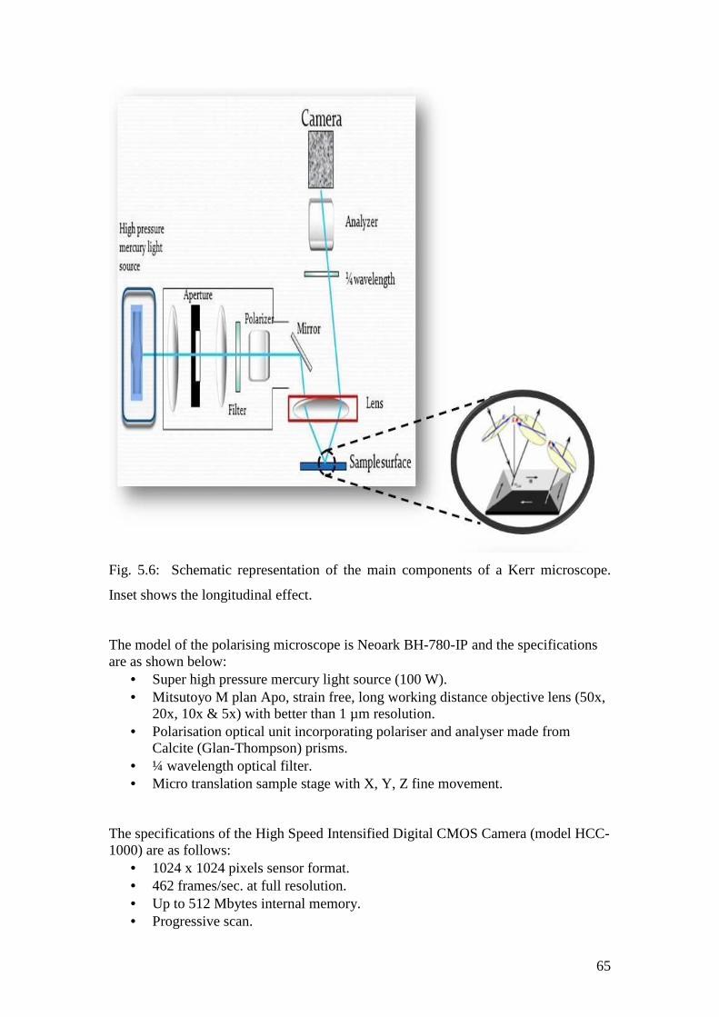
65

Fig. 5.6: Schematic representation of the main components of a Kerr microscope.

Inset shows the longitudinal effect.

The model of the polarising microscope is Neoark BH-780-IP and the specifications are as shown below:

• Super high pressure mercury light source (100 W). • Mitsutoyo M plan Apo, strain free, long working distance objective lens (50x,

20x, 10x & 5x) with better than 1 µm resolution. • Polarisation optical unit incorporating polariser and analyser made from

Calcite (Glan-Thompson) prisms. • ¼ wavelength optical filter. • Micro translation sample stage with X, Y, Z fine movement.

The specifications of the High Speed Intensified Digital CMOS Camera (model HCC-1000) are as follows:

• 1024 x 1024 pixels sensor format. • 462 frames/sec. at full resolution. • Up to 512 Mbytes internal memory. • Progressive scan.

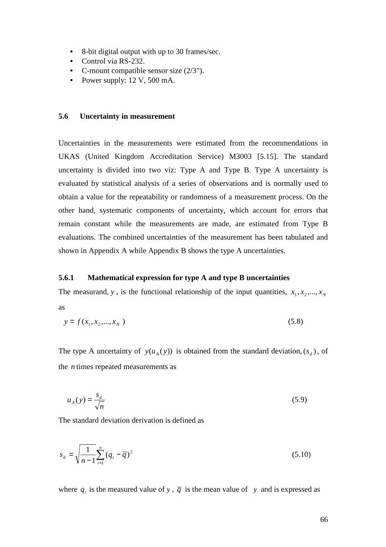
66

• 8-bit digital output with up to 30 frames/sec. • Control via RS-232. • C-mount compatible sensor size (2/3"). • Power supply: 12 V, 500 mA.

5.6 Uncertainty in measurement

Uncertainties in the measurements were estimated from the recommendations in

UKAS (United Kingdom Accreditation Service) M3003 [5.15]. The standard

uncertainty is divided into two viz: Type A and Type B. Type A uncertainty is

evaluated by statistical analysis of a series of observations and is normally used to

obtain a value for the repeatability or randomness of a measurement process. On the

other hand, systematic components of uncertainty, which account for errors that

remain constant while the measurements are made, are estimated from Type B

evaluations. The combined uncertainties of the measurement has been tabulated and

shown in Appendix A while Appendix B shows the type A uncertainties.

5.6.1 Mathematical expression for type A and type B uncertainties

The measurand,y , is the functional relationship of the input quantities, Nxxx ,...,, 21

as

Nxxxfy ,...,,( 21= ) (5.8)

The type A uncertainty of ))(( yuy A is obtained from the standard deviation, )( ds , of

the n times repeated measurements as

n

syu d

A =)( (5.9)

The standard deviation derivation is defined as

2

1

)(1

1qq

ns

n

iid −

−= ∑

=

(5.10)

where iq is the measured value ofy , q is the mean value of y and is expressed as

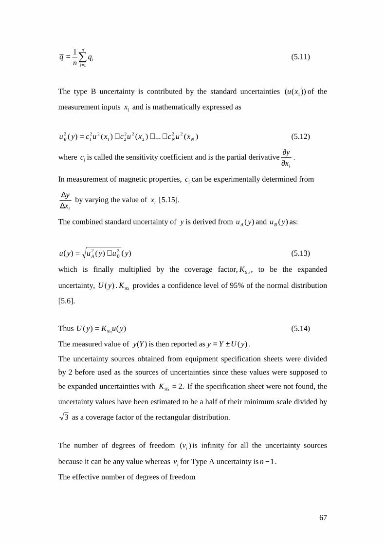
67

∑=

=n

iiq

nq

1

1 (5.11)

The type B uncertainty is contributed by the standard uncertainties ))(( 1xu of the

measurement inputs 1x and is mathematically expressed as

)(...)()()( 222

2221

221

2NNB xucxucxucyu +++= (5.12)

where ic is called the sensitivity coefficient and is the partial derivativeix

y

∂∂

.

In measurement of magnetic properties, ic can be experimentally determined from

ix

y

∆∆

by varying the value of ix [5.15].

The combined standard uncertainty of y is derived from )(yuA and )(yuB as:

)()()( 22 yuyuyu BA += (5.13)

which is finally multiplied by the coverage factor,95K , to be the expanded

uncertainty, )(yU . 95K provides a confidence level of 95% of the normal distribution

[5.6].

Thus )()( 95 yuKyU = (5.14)

The measured value of )(Yy is then reported as )(yUYy ±= .

The uncertainty sources obtained from equipment specification sheets were divided

by 2 before used as the sources of uncertainties since these values were supposed to

be expanded uncertainties with .295 =K If the specification sheet were not found, the

uncertainty values have been estimated to be a half of their minimum scale divided by

3 as a coverage factor of the rectangular distribution.

The number of degrees of freedom )( iv is infinity for all the uncertainty sources

because it can be any value whereas iv for Type A uncertainty is 1−n .

The effective number of degrees of freedom

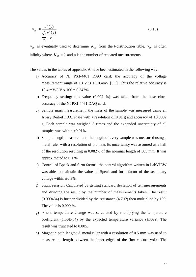
68

∑=

=n

i i

ieff

v

yv

yuv

1

4

4

)(

)( (5.15)

effv is eventually used to determine 95K from the t-distribution table. effv is often

infinity where 295 =K and n is the number of repeated measurements.

The values in the tables of appendix A have been estimated in the following way:

a) Accuracy of NI PXI-4461 DAQ card: the accuracy of the voltage

measurement range of ±3 V is ± 10.4mV [5.3]. Thus the relative accuracy is

10.4 mV/3 V x 100 = 0.347%

b) Frequency setting: this value (0.002 %) was taken from the base clock

accuracy of the NI PXI-4461 DAQ card.

c) Sample mass measurement: the mass of the sample was measured using an

Avery Berkel FB31 scale with a resolution of 0.01 g and accuracy of ±0.0002

g. Each sample was weighed 5 times and the expanded uncertainty of all

samples was within ±0.01%.

d) Sample length measurement: the length of every sample was measured using a

metal ruler with a resolution of 0.5 mm. Its uncertainty was assumed as a half

of the resolution resulting in 0.082% of the nominal length of 305 mm. It was

approximated to 0.1 %.

e) Control of Bpeak and form factor: the control algorithm written in LabVIEW

was able to maintain the value of Bpeak and form factor of the secondary

voltage within ±0.3%.

f) Shunt resistor: Calculated by getting standard deviation of ten measurements

and dividing the result by the number of measurements taken. The result

(0.000434) is further divided by the resistance (4.7 Ω) then multiplied by 100.

The value is 0.009 %.

g) Shunt temperature change was calculated by multiplying the temperature

coefficient (1.50E-04) by the expected temperature variance (±30%). The

result was truncated to 0.005.

h) Magnetic path length: A metal ruler with a resolution of 0.5 mm was used to

measure the length between the inner edges of the flux closure yoke. The

69

nominal length is 270 mm, so the relative uncertainty was 0.25 mm/270 mm x

100 = 0.093 %, rounded to 0.1 %.

i) Density: The quoted value is 7650 kg/m^3. The uncertainty is presumably a

half of the last digit of the quoted value which is ±0.0025. This yields a

relative value of 0.033%.

j) Type A uncertainty was derived from the standard deviation of 3 times

repeated measurements of each sample tested.

k) Accuracy of the strain amplifier: The gain of the strain amplifier of the Vishay

system 3800 has a resolution of 0.05% [5.9].

l) Accuracy of the shunt calibration resistors: The shunt calibration resistors of

the strain indicator of the Vishay system 3800 have the accuracy of ±0.05 Ω.

m) Width of the sample: the sample width was measured by means of a digital

veneer calliper having an accuracy of 0.02 mm. It is 0.067 of the nominal

value at the nominal value of 30 mm. It is approximated to 0.07%.

n) Thickness of the sample: A digital micrometer was used to measure the

thickness and its accuracy was 0.0025 mm, which is 0.83% of the 0.30 mm

thick sample.

o) Gauge factor: the uncertainty of the gain factor is ±1% [5.7].

p) Jaw gripping: The sample has the tendency of slipping slightly at the start of

applying tensile stress. It was difficult to quantify this effect, so the

uncertainty of ±2.5% was estimated [5.6].

70



magnetostriction in grain-oriented silicon iron, PhD thesis, Cardiff University

2003.

[5.2] K. Hartmann, A.J. Moses and T. Meydan, A system for measurement of AC

Barkhausen noise in electrical steels, Journal of Magnetism and Magnetic

Materials Vol. 254–255, pp. 318–320, 2003.

[5.3] National Instruments, Dynamic signal acquisition user manual, August 2002.

[5.4] BS EN 10280:2001 + A1:2007, Magnetic Materials- Methods of

measurement of the magnetic properties of electrical sheet and strip by means of a

single sheet tester, British Standard, 2007.

[5.5] S. Zurek, P. Marketos, P. I. Anderson, and A. J Moses, Influence of digital

resolution of measuring equipment on the accuracy of power loss measured in

Epstein frame, Przeglad Elektrotechniczny (Electrical Reviews), Vol. R. 83, pp.

50-53, 2007.

[5.6] S. Somkun, Magnetostriction and magnetic anisotropy in non oriented

electrical steel and stator core laminations, PhD thesis, Cardiff University,

September 2010.

[5.7] (www.omega.com/techref/pdf/strain-gage-technicaldata.pdf). Strain gauge

technical data manufacturer’smanual. Accessed on 15th July 2011.

[5.8] Omega, SG496 Rapid Cure Strain Gauge Adhesives User’s Guides, 2008.

[5.9] Instruction manual of model 3800 wide range strain indicator.

[5.10] P. Klimcyzk, Novel technique for characterisation and control of

magnetostriction in grain oriented silicon steel, PhD thesis, Cardiff University,

2012.

[5.11] B. Fukuda, K. Satoh, T. Ichida, Y. Itoh, and H. Shimanaka, Effect of surface

coatings on domain structure in grain oriented 3% Si-Fe, IEEE Transactions on

Magnetics, Vol.17, No.6, pp. 2878-2880, 1981.

[5.12] A. Hubert and R. Schäfer, Magnetic Domains. Berlin, Germany, Springer-

Verlag, 1998.

[5.13] J. Kerr, On rotation of the plane of polarization by reflection from the pole

of a magnet, Philosophical Magazine, Vol. 3, pp.321–343, 1877.

71

[5.14]http://www.ece.neu.edu/faculty/dimarzio/capstone/samples/Final%20Capsto

ne%20Report.pdf. Accessed on 20th July, 2011.

[5.15] UKAS M3003, The expression of uncertainty and confidence in

measurement, 1997.

72

Chapter 6 Investigation of magnetic properties

and Barkhausen noise of grain oriented electrical

steel

6.1 Introduction

The experimental results obtained on the strips of CGO and HGO steels using the

measurement equipment described in section 5.2 are presented in this chapter.

Measurements of coercivity, B-H loop, AC relative permeability and specific power

loss are presented and discussed. Experimental measurements of BN of the test

samples at high and low flux densities are also presented and discussed.

An average of 3 measurements made on every strip was used in analysing the result.

Between repeatability measurements each sample was removed and then re-inserted

into the test system. The percentage difference of the measured properties was

quantified using equation 6.1. The actual difference could be positive or negative

depending on the values of the measured parameters under consideration. The

parameters quantified are the rms, TSA, coercivity, relative permeability and power

loss. The actual difference is the result of subtracting the one value of a parameter

from another value of the same parameter in the different samples under

consideration. The subtrahend is the ‘original value’ in equation 6.1.

% Difference = Actual difference/Original value x 100 % (6.1)

6.2 B-H loops, coercivity, relative permeability and specific power loss of CGO

and HGO

This part of the investigation was carried out on samples of HGO and CGO steels,

305 mm x 30 mm x 0.27 mm from Cogent Power Limited United Kingdom. 40 strips

comprising 20 CGO and 20 HGO were tested. The HGO and CGO strips had average

grain sizes of 9 mm and 4 mm respectively. Each strip was singly magnetised under

sinusoidal peak flux density from 8.0 mT to 1.5 T at a magnetising frequency of 50

Hz. The uncertainty of measurement for the peak flux density and peak magnetic field

at low and high flux densities are shown in tables A1-A3.

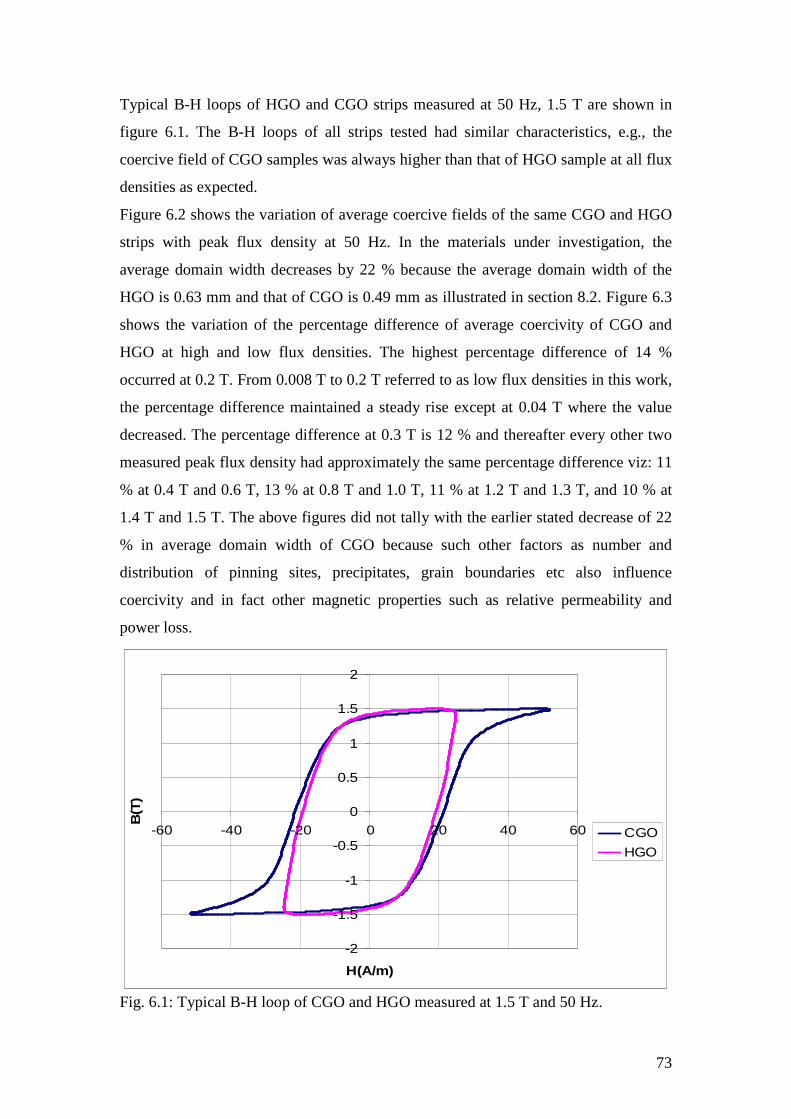
73

Typical B-H loops of HGO and CGO strips measured at 50 Hz, 1.5 T are shown in

figure 6.1. The B-H loops of all strips tested had similar characteristics, e.g., the

coercive field of CGO samples was always higher than that of HGO sample at all flux

densities as expected.

Figure 6.2 shows the variation of average coercive fields of the same CGO and HGO

strips with peak flux density at 50 Hz. In the materials under investigation, the

average domain width decreases by 22 % because the average domain width of the

HGO is 0.63 mm and that of CGO is 0.49 mm as illustrated in section 8.2. Figure 6.3

shows the variation of the percentage difference of average coercivity of CGO and

HGO at high and low flux densities. The highest percentage difference of 14 %

occurred at 0.2 T. From 0.008 T to 0.2 T referred to as low flux densities in this work,

the percentage difference maintained a steady rise except at 0.04 T where the value

decreased. The percentage difference at 0.3 T is 12 % and thereafter every other two

measured peak flux density had approximately the same percentage difference viz: 11

% at 0.4 T and 0.6 T, 13 % at 0.8 T and 1.0 T, 11 % at 1.2 T and 1.3 T, and 10 % at

1.4 T and 1.5 T. The above figures did not tally with the earlier stated decrease of 22

% in average domain width of CGO because such other factors as number and

distribution of pinning sites, precipitates, grain boundaries etc also influence

coercivity and in fact other magnetic properties such as relative permeability and

power loss.

-2

-1.5

-1

-0.5

0

0.5

1

1.5

2

-60 -40 -20 0 20 40 60

H(A/m)

B(T

)

CGO

HGO

Fig. 6.1: Typical B-H loop of CGO and HGO measured at 1.5 T and 50 Hz.

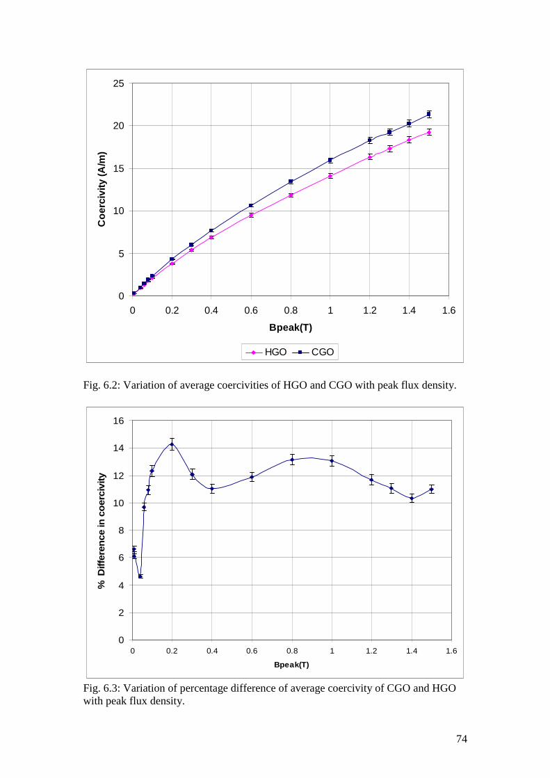
74

0

5

10

15

20

25

0 0.2 0.4 0.6 0.8 1 1.2 1.4 1.6

Bpeak(T)

Co

erci

vity

(A/m

)

HGO CGO

Fig. 6.2: Variation of average coercivities of HGO and CGO with peak flux density.

0

2

4

6

8

10

12

14

16

0 0.2 0.4 0.6 0.8 1 1.2 1.4 1.6

Bpeak(T)

% D

iffer

ence

in c

oer

civi

ty

Fig. 6.3: Variation of percentage difference of average coercivity of CGO and HGO with peak flux density.

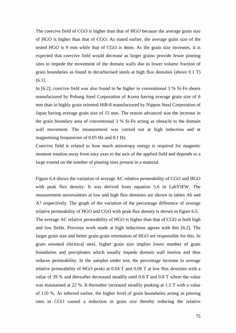
75

The coercive field of CGO is higher than that of HGO because the average grain size

of HGO is higher than that of CGO. As stated earlier, the average grain size of the

tested HGO is 9 mm while that of CGO is 4mm. As the grain size increases, it is

expected that coercive field would decrease as larger grains provide fewer pinning

sites to impede the movement of the domain walls due to lower volume fraction of

grain boundaries as found in decarburised steels at high flux densities (above 0.1 T)

[6.1].

In [6.2], coercive field was also found to be higher in conventional 3 % Si-Fe sheets

manufactured by Pohang Steel Corporation of Korea having average grain size of 6

mm than in highly grain oriented HiB-8 manufactured by Nippon Steel Corporation of

Japan having average grain size of 15 mm. The reason advanced was the increase in

the grain boundary area of conventional 3 % Si-Fe acting as obstacle to the domain

wall movement. The measurement was carried out at high induction and at

magnetising frequencies of 0.05 Hz and 0.1 Hz.

Coercive field is related to how much anisotropy energy is required for magnetic

moment rotation away from easy axes to the axis of the applied field and depends to a

large extend on the number of pinning sites present in a material.

Figure 6.4 shows the variation of average AC relative permeability of CGO and HGO

with peak flux density. It was derived from equation 5.6 in LabVIEW. The

measurement uncertainties at low and high flux densities are shown in tables A6 and

A7 respectively. The graph of the variation of the percentage difference of average

relative permeability of HGO and CGO with peak flux density is shown in figure 6.5.

The average AC relative permeability of HGO is higher than that of CGO at both high

and low fields. Previous work made at high inductions agrees with this [6.2]. The

larger grain size and better grain-grain orientation of HGO are responsible for this. In

grain oriented electrical steel, higher grain size implies lower number of grain

boundaries and precipitates which usually impede domain wall motion and thus

reduces permeability. In the samples under test, the percentage increase in average

relative permeability of HGO peaks at 0.04 T and 0.06 T at low flux densities with a

value of 39 % and thereafter decreased steadily until 0.6 T and 0.8 T where the value

was maintained at 22 %. It thereafter increased steadily peaking at 1.5 T with a value

of 110 %. As inferred earlier, the higher level of grain boundaries acting as pinning

sites in CGO caused a reduction in grain size thereby reducing the relative

76

permeability. Magnetic characterisation of grain oriented electrical steel is normally

measured at high inductions (1.5 T/ 1.7 T) [6.3] which is suitable for its typical

application in power transformers. For a given magnetic material, the permeability is

not usually specified over the low flux density range applicable in current transformer

cores and other applications where electrical steel is used at low flux densities. Recent

work at below 1mT [6.4] shows the permeability of CGO is higher than that of HGO

at this regime and confirms that performance at low magnetisation level cannot be

predicted from measurements made at high inductions especially when comparing the

performance of CGO and HGO.

77

0

5

10

15

20

25

30

35

40

45

50

0 0.3 0.6 0.9 1.2 1.5

Bpeak(T)

Rel

ativ

e per

mea

bili

ty (x

100

0)

HGO CGO

Fig. 6.4: Variation of average AC relative permeability of HGO and CGO with peak

flux density.

0

20

40

60

80

100

120

0 0.3 0.6 0.9 1.2 1.5Bpeak(T)

% D

iffer

ence

in r

elat

ive

per

mea

bili

ty

Fig. 6.5: Variation of percentage difference of average relative permeability of HGO

and CGO with peak flux density.

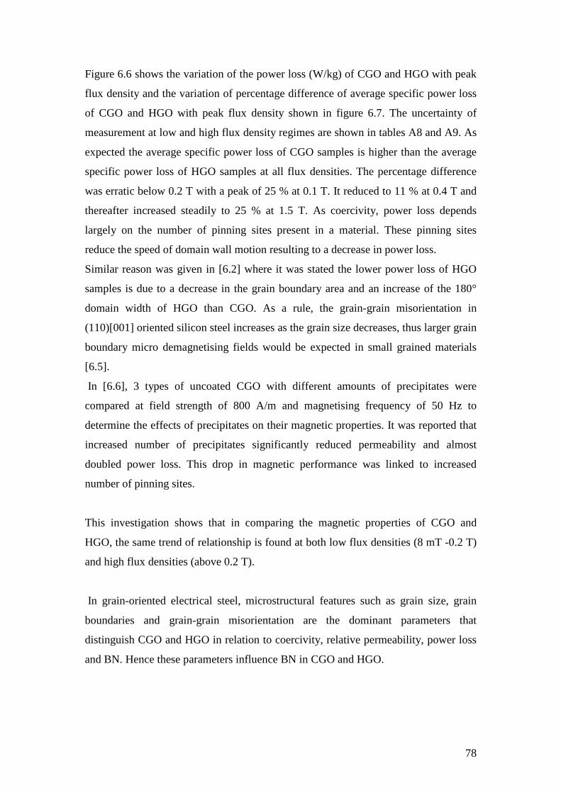
78

Figure 6.6 shows the variation of the power loss (W/kg) of CGO and HGO with peak

flux density and the variation of percentage difference of average specific power loss

of CGO and HGO with peak flux density shown in figure 6.7. The uncertainty of

measurement at low and high flux density regimes are shown in tables A8 and A9. As

expected the average specific power loss of CGO samples is higher than the average

specific power loss of HGO samples at all flux densities. The percentage difference

was erratic below 0.2 T with a peak of 25 % at 0.1 T. It reduced to 11 % at 0.4 T and

thereafter increased steadily to 25 % at 1.5 T. As coercivity, power loss depends

largely on the number of pinning sites present in a material. These pinning sites

reduce the speed of domain wall motion resulting to a decrease in power loss.

Similar reason was given in [6.2] where it was stated the lower power loss of HGO

samples is due to a decrease in the grain boundary area and an increase of the 180°

domain width of HGO than CGO. As a rule, the grain-grain misorientation in

(110)[001] oriented silicon steel increases as the grain size decreases, thus larger grain

boundary micro demagnetising fields would be expected in small grained materials

[6.5].

In [6.6], 3 types of uncoated CGO with different amounts of precipitates were

compared at field strength of 800 A/m and magnetising frequency of 50 Hz to

determine the effects of precipitates on their magnetic properties. It was reported that

increased number of precipitates significantly reduced permeability and almost

doubled power loss. This drop in magnetic performance was linked to increased

number of pinning sites.

This investigation shows that in comparing the magnetic properties of CGO and

HGO, the same trend of relationship is found at both low flux densities (8 mT -0.2 T)

and high flux densities (above 0.2 T).

In grain-oriented electrical steel, microstructural features such as grain size, grain

boundaries and grain-grain misorientation are the dominant parameters that

distinguish CGO and HGO in relation to coercivity, relative permeability, power loss

and BN. Hence these parameters influence BN in CGO and HGO.

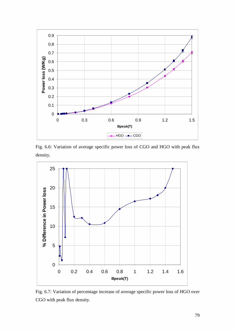
79

0

0.1

0.2

0.3

0.4

0.5

0.6

0.7

0.8

0.9

0 0.3 0.6 0.9 1.2 1.5Bpeak(T)

Po

wer

loss

(W/K

g)

HGO CGO

Fig. 6.6: Variation of average specific power loss of CGO and HGO with peak flux

density.

0

5

10

15

20

25

0 0.2 0.4 0.6 0.8 1 1.2 1.4 1.6Bpeak(T)

% D

iffer

ence

in P

ow

er lo

ss

Fig. 6.7: Variation of percentage increase of average specific power loss of HGO over

CGO with peak flux density.

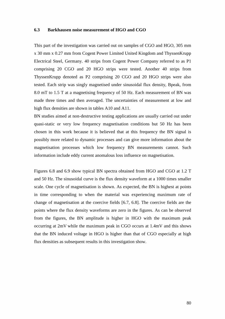
80

6.3 Barkhausen noise measurement of HGO and CGO

This part of the investigation was carried out on samples of CGO and HGO, 305 mm

x 30 mm x 0.27 mm from Cogent Power Limited United Kingdom and ThyssenKrupp

Electrical Steel, Germany. 40 strips from Cogent Power Company referred to as P1

comprising 20 CGO and 20 HGO strips were tested. Another 40 strips from

ThyssenKrupp denoted as P2 comprising 20 CGO and 20 HGO strips were also

tested. Each strip was singly magnetised under sinusoidal flux density, Bpeak, from

8.0 mT to 1.5 T at a magnetising frequency of 50 Hz. Each measurement of BN was

made three times and then averaged. The uncertainties of measurement at low and

high flux densities are shown in tables A10 and A11.

BN studies aimed at non-destructive testing applications are usually carried out under

quasi-static or very low frequency magnetisation conditions but 50 Hz has been

chosen in this work because it is believed that at this frequency the BN signal is

possibly more related to dynamic processes and can give more information about the

magnetisation processes which low frequency BN measurements cannot. Such

information include eddy current anomalous loss influence on magnetisation.

Figures 6.8 and 6.9 show typical BN spectra obtained from HGO and CGO at 1.2 T

and 50 Hz. The sinusoidal curve is the flux density waveform at a 1000 times smaller

scale. One cycle of magnetisation is shown. As expected, the BN is highest at points

in time corresponding to when the material was experiencing maximum rate of

change of magnetisation at the coercive fields [6.7, 6.8]. The coercive fields are the

points where the flux density waveforms are zero in the figures. As can be observed

from the figures, the BN amplitude is higher in HGO with the maximum peak

occurring at 2mV while the maximum peak in CGO occurs at 1.4mV and this shows

that the BN induced voltage in HGO is higher than that of CGO especially at high

flux densities as subsequent results in this investigation show.

81

0 2 4 6 8 10 12 14 16 18 20-2

-1.5

-1

-0.5

0

0.5

1

1.5

2x 10

-3

time (mS)

Bar

khau

sen

no

ise

amp

(V)

BN

B/(1000)T

Fig.6.8: BN spectrum of HGO during one cycle of magnetisation at 1.2 T and 50 Hz

showing variation of BN amplitude with time.

0 2 4 6 8 10 12 14 16 18 20-2

-1.5

-1

-0.5

0

0.5

1

1.5

2x 10

-3

time (mS)

Bar

khau

sen

no

ise

amp

(V)

BN

B(/1000)T

Fig. 6.9: BN spectrum of CGO during one cycle of magnetisation at 1.2 T and 50 Hz

showing variation of BN amplitude with time.

82

Figure 6.10 shows the rms values of the BN spectra shown in figures 6.8 and 6.9 as

well as the background noise of the experimental set up at all the peak flux densities

measured. Preliminary test determined the background noise level in the experimental

set up. The same relationship was obtained when the background noise was plotted

against the total sum of amplitudes (TSA) and total number of points (TNP). It can be

observed from the figure that the background noise is more than 100 times less that

the BN amplitude of the test samples. This was achieved by applying all the

background noise reduction techniques discussed in section 5.3. Background noise

reduction is particularly challenging at very low inductions and measurements must

be made in an environment free from electromagnetic interference.

0

0.1

0.2

0.3

0.4

0.5

0.6

0 0.3 0.6 0.9 1.2 1.5

Bpeak(T)

RM

S o

f bac

kgro

un

d n

ois

e (m

V)

BNrms of HGO BNrms of CGO RMS of background noise

Fig. 6.10: Comparison of average rms BN of CGO and HGO strips at different flux

densities at 50 Hz with background noise of Experimental set-up.

Figure 6.11 shows the variation of average rms BN of 20 strips of CGO and 20 strips

of HGO from P1 at both high and low flux densities. It can be observed that the

average rms BN is higher in HGO than in CGO above 0.2 T but at lower flux

densities the trend changes. A similar characteristic was obtained when the same

number of test samples from P2 was investigated at both magnetisation regimes. This

is shown in figure 6.12. The variation of the percentage difference of the average rms

BN of these test samples with peak flux density is shown in figure 6.13.

83

Figure 6.14 shows the same BN signals expressed in terms of the average TSA of BN

peaks of the test samples from P1. As with the rms BN, the TSA of HGO is higher

than that of CGO above 0.2 T and the trend changes at lower flux densities. TSA of

samples from P2 show the same relationship as with P1 and is plotted in figure 6.15

with the variation in percentage difference at both high and low flux densities shown

in figure 6.16.

84

0

0.1

0.2

0.3

0.4

0.5

0.6

0.7

0 0.3 0.6 0.9 1.2 1.5

Bpeak(T)

BN

rms(

mV

)

CGO HGO

(a)

0

0.01

0.02

0.03

0.04

0.05

0.06

0.07

0 0.05 0.1 0.15 0.2

Bpeak(T)

BN

rms

(mV

)

CGO HGO

(b)

Fig. 6.11: (a) Variation of average rms BN of 20 strips each of CGO and HGO from

P1 with peak flux density (b) the same comparison in the low field regime.

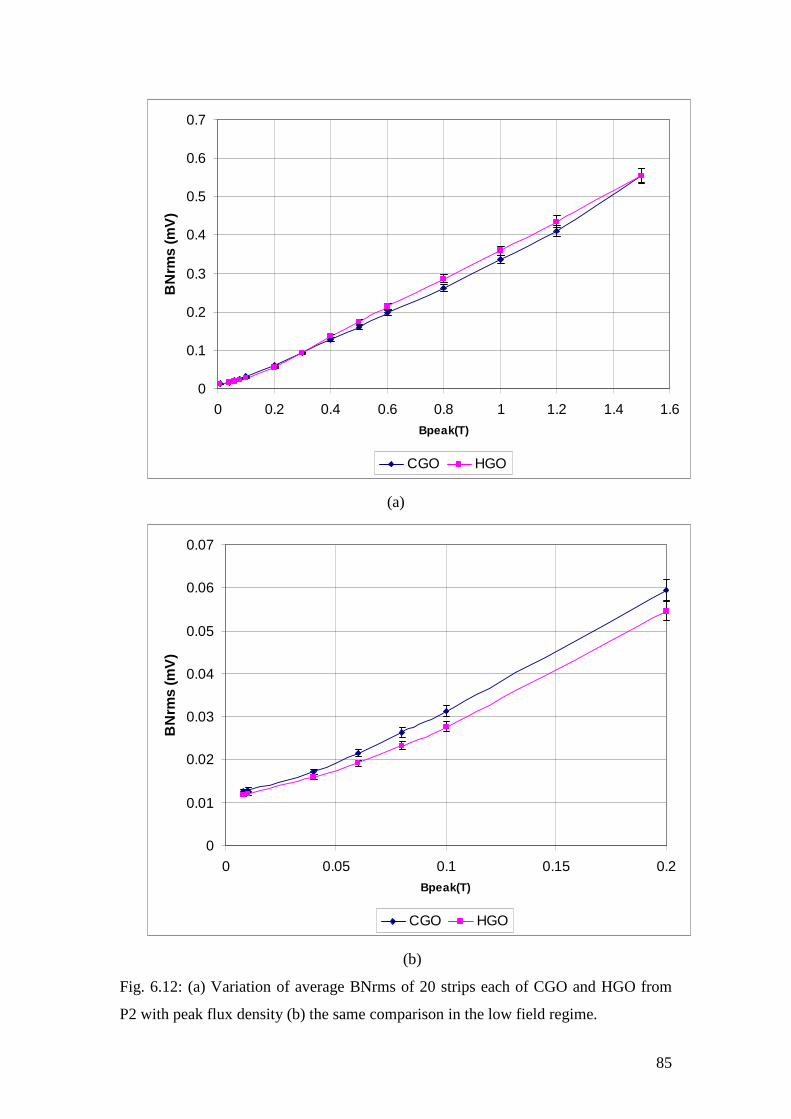
85

0

0.1

0.2

0.3

0.4

0.5

0.6

0.7

0 0.2 0.4 0.6 0.8 1 1.2 1.4 1.6Bpeak(T)

BN

rms

(mV

)

CGO HGO

(a)

0

0.01

0.02

0.03

0.04

0.05

0.06

0.07

0 0.05 0.1 0.15 0.2Bpeak(T)

BN

rms

(mV

)

CGO HGO

(b)

Fig. 6.12: (a) Variation of average BNrms of 20 strips each of CGO and HGO from

P2 with peak flux density (b) the same comparison in the low field regime.

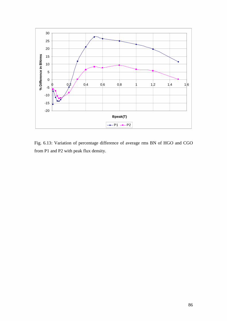
86

-20

-15

-10

-5

0

5

10

15

20

25

30

0 0.2 0.4 0.6 0.8 1 1.2 1.4 1.6

Bpeak(T)

% D

iffer

ence

in B

Nrm

s

P1 P2

Fig. 6.13: Variation of percentage difference of average rms BN of HGO and CGO

from P1 and P2 with peak flux density.

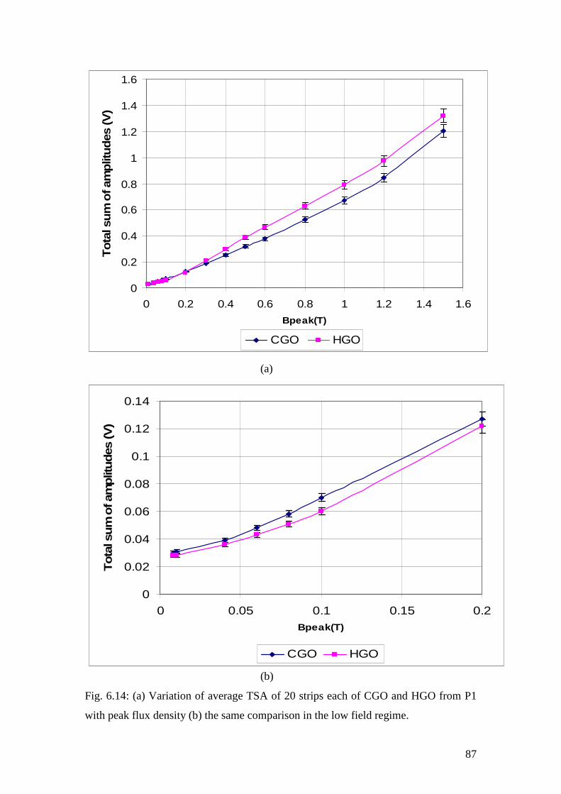
87

0

0.2

0.4

0.6

0.8

1

1.2

1.4

1.6

0 0.2 0.4 0.6 0.8 1 1.2 1.4 1.6

Bpeak(T)

To

tal s

um

of a

mp

litu

des

(V)

CGO HGO

(a)

0

0.02

0.04

0.06

0.08

0.1

0.12

0.14

0 0.05 0.1 0.15 0.2Bpeak(T)

Tota

l sum

of a

mplit

udes

(V)

CGO HGO

(b)

Fig. 6.14: (a) Variation of average TSA of 20 strips each of CGO and HGO from P1

with peak flux density (b) the same comparison in the low field regime.

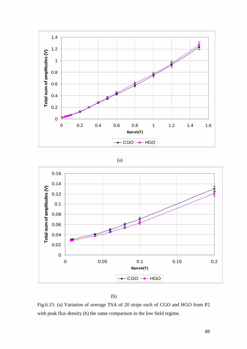
88

0

0.2

0.4

0.6

0.8

1

1.2

1.4

0 0.2 0.4 0.6 0.8 1 1.2 1.4 1.6Bpeak(T)

To

tal s

um

of a

mp

litu

des

(V)

CGO HGO

(a)

0

0.02

0.04

0.06

0.08

0.1

0.12

0.14

0.16

0 0.05 0.1 0.15 0.2Bpeak(T)

To

tal s

um

of a

mp

litu

des

(V)

CGO HGO

(b)

Fig.6.15: (a) Variation of average TSA of 20 strips each of CGO and HGO from P2

with peak flux density (b) the same comparison in the low field regime.

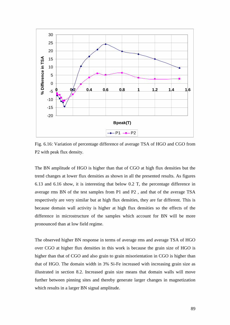
89

-20

-15

-10

-5

0

5

10

15

20

25

30

0 0.2 0.4 0.6 0.8 1 1.2 1.4 1.6

Bpeak(T)

% D

iffer

ence

in T

SA

P1 P2

Fig. 6.16: Variation of percentage difference of average TSA of HGO and CGO from

P2 with peak flux density.

The BN amplitude of HGO is higher than that of CGO at high flux densities but the

trend changes at lower flux densities as shown in all the presented results. As figures

6.13 and 6.16 show, it is interesting that below 0.2 T, the percentage difference in

average rms BN of the test samples from P1 and P2 , and that of the average TSA

respectively are very similar but at high flux densities, they are far different. This is

because domain wall activity is higher at high flux densities so the effects of the

difference in microstructure of the samples which account for BN will be more

pronounced than at low field regime.

The observed higher BN response in terms of average rms and average TSA of HGO

over CGO at higher flux densities in this work is because the grain size of HGO is

higher than that of CGO and also grain to grain misorientation in CGO is higher than

that of HGO. The domain width in 3% Si-Fe increased with increasing grain size as

illustrated in section 8.2. Increased grain size means that domain walls will move

further between pinning sites and thereby generate larger changes in magnetization

which results in a larger BN signal amplitude.

90

Secondly, the grain-grain misorientation which is higher in CGO [6.9, 6.10] results in

strong depression of the BN level which is caused by a decrease in the instantaneous

rate of change of the magnetic flux during Barkhausen jumps, because of increased

demagnetizing effects.

Similar results were found at high flux densities in decarburised steel [6.1], carbon

steel [6.11], high purity iron [6.12] and grain oriented electrical steel from Nippon

Steel Corporation and Pohang Steel Corporation [6.2]. The reason advanced in [6.2]

for the lower BN amplitude of CGO compared to HGO is the larger energy loss in

CGO due to domain nucleation and annihilation.

However, contradictory result was obtained [6.13] when the BN was measured at 50

Hz and peak flux densities of 0.5 T- 1.4 T in 3 Epstein sized samples comprising of

0.27 mm thick HGO with average grain size of 13 mm, 0.27 mm thick CGO with

average grain size of 8 mm, and 0.20 mm thick, 0.1 % silicon NGO with average

grain size of 100µm. The investigation showed that the BN amplitude is higher for the

material with a smaller grain size.

This apparent contradiction suggests that the BN process is more complex and the

results might be associated with materials having different densities of pinning sites,

precipitates , grain boundaries, etc possibly higher in smaller grain materials.

BN measurement has not been carried out at low flux densities (below 0.1 T) before.

At low fields, domain wall motion has an intermittent, jerky character, with sparse

Barkhausen jumps. The implication of this is that smaller grain samples (CGO) which

have more grain boundaries acting as pinning sites and hence large fractional volume

than HGO will have a greater number of these sparse Barkhausen jumps which will

sum up to higher Barkhausen noise amplitude. This explains why at low flux density,

the BN amplitude is higher in CGO material. This investigation shows that in

comparing CGO and HGO, BN amplitude changes trend at high and low flux

densities.

91


[6.1] R. Ranjan, D. C. Jiles and P. K. Rastogi, Magnetic properties of decarburized


Transactions on Magnetics, Vol. 23 , No. 3, pp.1869-1876, 1987.

[6.2] D. G. Hwang, H.C. Kim, C. G. Kim, K.A Lee, Barkhausen noise and magnetic

properties of highly grain-oriented HiB-8 and conventional 3% Si-Fe polycrystalline

specimens, Journal of Korean Physical Society, Vol. 24, No.6, pp. 493-498, 1991.

[6.3] International Electrotechnical Commission (IEC) Standard 6044-1, 1996.

[6.4] T. Kutrowski, Characterisation of metering transformer cores, PhD thesis,

Cardiff University (to be submitted, 2012).


grain-oriented 3% Si-Fe, IEEE Transactions on Magnetics, Vol. 10, No. 2, 195-222,

1974.

[6.6] S. Turner, A. Moses, J. Hall and K. Jenkins, The effect of precipitate size on


Physics, Vol.107, issue 3, pp. 307-309, 2010.

[6.7] H.V. Patel, S. Zurek, T. Meydan, D.C Jiles and L. LI, A new adaptive automated

feedback system for Barkhausen signal measurement, Sensors and Actuators A , Vol.

129, pp.112-117, 2006.


Magnetostriction in Grain-oriented silicon iron, PhD thesis, Cardiff University, March

2003.

[6.9] S. Taguchi, A. Sakakura and H. Takashima, US Patent 3287183, 1966.

[6.10] M. F. Littmann, Structures and magnetic properties of grain oriented 3.2%

silicon-iron, Journal of Applied Physics, Vol. 38, issue 3, pp. 1104-1108, 1967.

[6.11] H. Sakamoto, M. Okada and M. Homma, Theoretical analysis of Barkhausen

noise in carbon steel, IEEE Transactions on Magnetics, Vol. 23 No.5, pp. 2236-2238,

1987.

[6.12] J. Degaulque, B. Astie, J. L. Porteseil and R Vergne, Predictions of the random

potential energy models of domain wall motion, An experimental investigation of

high purity iron, Journal of Magnetism and Magnetic Materials, Vol. 128, issue 1-2,

pp. 149-153, 1982.

92

[6.13] K. Hartmann, A.J. Moses and T. Meydan, A system for measurement of AC

Barkhausen noise in electrical steels, Journal of Magnetism and Magnetic Materials

Vol. 254–255, pp. 318–320, 2003.

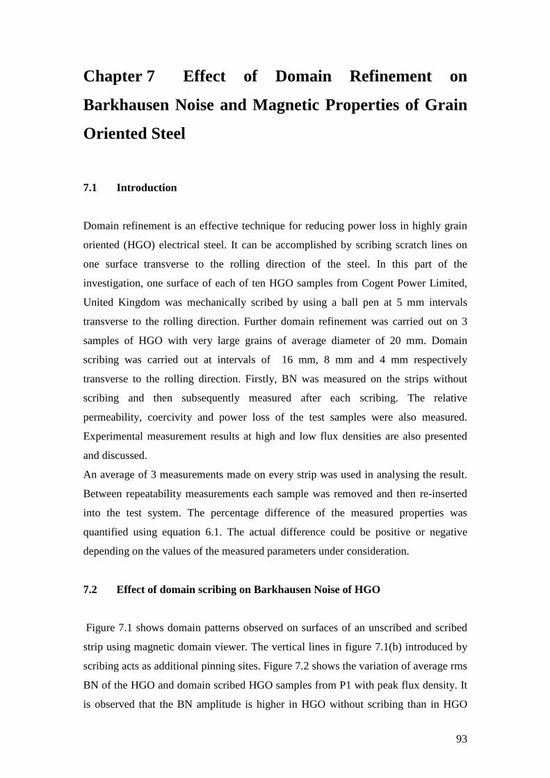
93

Chapter 7 Effect of Domain Refinement on

Barkhausen Noise and Magnetic Properties of Grain

Oriented Steel

7.1 Introduction

Domain refinement is an effective technique for reducing power loss in highly grain

oriented (HGO) electrical steel. It can be accomplished by scribing scratch lines on

one surface transverse to the rolling direction of the steel. In this part of the

investigation, one surface of each of ten HGO samples from Cogent Power Limited,

United Kingdom was mechanically scribed by using a ball pen at 5 mm intervals

transverse to the rolling direction. Further domain refinement was carried out on 3

samples of HGO with very large grains of average diameter of 20 mm. Domain

scribing was carried out at intervals of 16 mm, 8 mm and 4 mm respectively

transverse to the rolling direction. Firstly, BN was measured on the strips without

scribing and then subsequently measured after each scribing. The relative

permeability, coercivity and power loss of the test samples were also measured.

Experimental measurement results at high and low flux densities are also presented

and discussed.

An average of 3 measurements made on every strip was used in analysing the result.

Between repeatability measurements each sample was removed and then re-inserted

into the test system. The percentage difference of the measured properties was

quantified using equation 6.1. The actual difference could be positive or negative

depending on the values of the measured parameters under consideration.

7.2 Effect of domain scribing on Barkhausen Noise of HGO

Figure 7.1 shows domain patterns observed on surfaces of an unscribed and scribed

strip using magnetic domain viewer. The vertical lines in figure 7.1(b) introduced by

scribing acts as additional pinning sites. Figure 7.2 shows the variation of average rms

BN of the HGO and domain scribed HGO samples from P1 with peak flux density. It

is observed that the BN amplitude is higher in HGO without scribing than in HGO

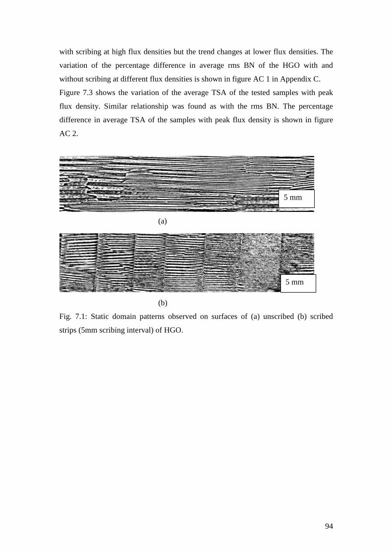
94

with scribing at high flux densities but the trend changes at lower flux densities. The

variation of the percentage difference in average rms BN of the HGO with and

without scribing at different flux densities is shown in figure AC 1 in Appendix C.

Figure 7.3 shows the variation of the average TSA of the tested samples with peak

flux density. Similar relationship was found as with the rms BN. The percentage

difference in average TSA of the samples with peak flux density is shown in figure

AC 2.

(a)

(b)

Fig. 7.1: Static domain patterns observed on surfaces of (a) unscribed (b) scribed

strips (5mm scribing interval) of HGO.

5 mm

5 mm

95

0

0.1

0.2

0.3

0.4

0.5

0.6

0 0.2 0.4 0.6 0.8 1 1.2 1.4Bpeak(T)

BN

rms

(mV

)

HGO Domain scribed HGO

(a)

0

0.02

0.04

0.06

0.08

0.1

0.12

0.14

0.16

0 0.05 0.1 0.15 0.2 0.25 0.3 0.35 0.4Bpeak(T)

BN

rms

(mV

)


(b)

Fig. 7.2: (a) Variation of average rms BN of 10 strips each of HGO and Domain-

scribed HGO from P1 with peak flux density (b) Comparison in the low field regime.

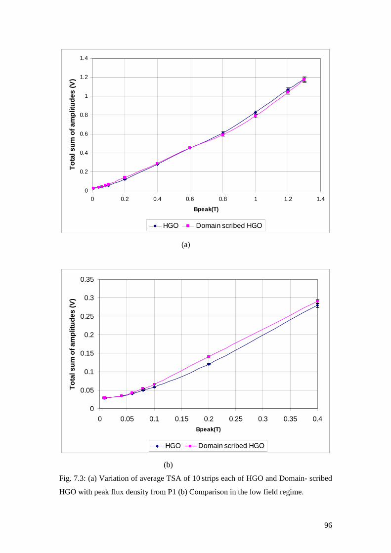
96

0

0.2

0.4

0.6

0.8

1

1.2

1.4

0 0.2 0.4 0.6 0.8 1 1.2 1.4

Bpeak(T)

To

tal s

um

of a

mp

litu

des

(V)


(a)

0

0.05

0.1

0.15

0.2

0.25

0.3

0.35

0 0.05 0.1 0.15 0.2 0.25 0.3 0.35 0.4Bpeak(T)

To

tal s

um

of a

mp

litu

des

(V)


(b)

Fig. 7.3: (a) Variation of average TSA of 10 strips each of HGO and Domain- scribed

HGO with peak flux density from P1 (b) Comparison in the low field regime.

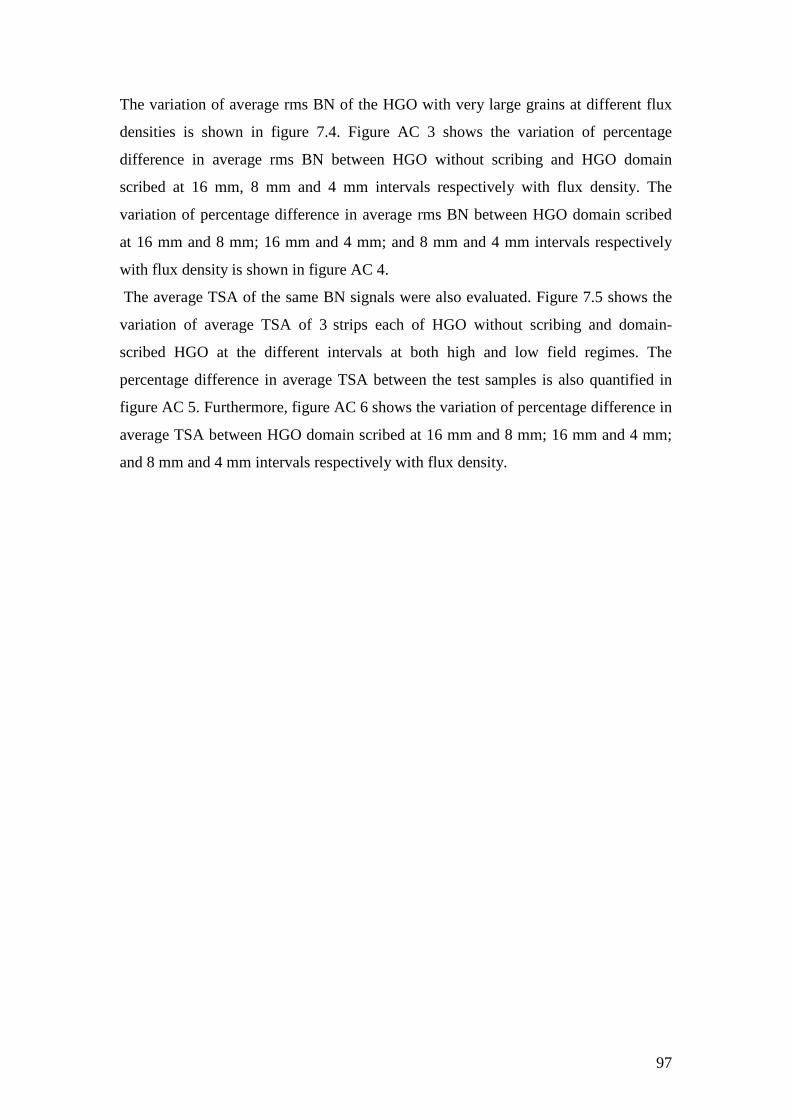
97

The variation of average rms BN of the HGO with very large grains at different flux

densities is shown in figure 7.4. Figure AC 3 shows the variation of percentage

difference in average rms BN between HGO without scribing and HGO domain

scribed at 16 mm, 8 mm and 4 mm intervals respectively with flux density. The

variation of percentage difference in average rms BN between HGO domain scribed

at 16 mm and 8 mm; 16 mm and 4 mm; and 8 mm and 4 mm intervals respectively

with flux density is shown in figure AC 4.

The average TSA of the same BN signals were also evaluated. Figure 7.5 shows the

variation of average TSA of 3 strips each of HGO without scribing and domain-

scribed HGO at the different intervals at both high and low field regimes. The

percentage difference in average TSA between the test samples is also quantified in

figure AC 5. Furthermore, figure AC 6 shows the variation of percentage difference in

average TSA between HGO domain scribed at 16 mm and 8 mm; 16 mm and 4 mm;

and 8 mm and 4 mm intervals respectively with flux density.

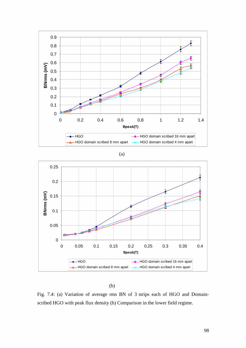
98

0

0.1

0.2

0.3

0.4

0.5

0.6

0.7

0.8

0.9

0 0.2 0.4 0.6 0.8 1 1.2 1.4Bpeak(T)

BN

rms

(mV

)

HGO HGO domain scribed 16 mm apart

HGO domain scribed 8 mm apart HGO domain scribed 4 mm apart

(a)

0

0.05

0.1

0.15

0.2

0.25

0 0.05 0.1 0.15 0.2 0.25 0.3 0.35 0.4Bpeak(T)

BN

rms

(mV

)



(b)

Fig. 7.4: (a) Variation of average rms BN of 3 strips each of HGO and Domain-

scribed HGO with peak flux density (b) Comparison in the lower field regime.

99

0

0.2

0.4

0.6

0.8

1

1.2

1.4

1.6

1.8

2

0 0.2 0.4 0.6 0.8 1 1.2 1.4Bpeak(T)

To

tal s

um

of a

mp

litu

des

(V)


HGO domainscribed 8 mm apart HGO domain scribed 4 mm apart

(a)

0

0.1

0.2

0.3

0.4

0.5

0.6

0 0.05 0.1 0.15 0.2 0.25 0.3 0.35 0.4Bpeak(T)

To

tal s

um

of a

mp

litu

des

(V)



(b)

Fig. 7.5:(a) Variation of average TSA of BN of 3 strips each of unscribed HGO and

domain-scribed HGO with peak flux density (b) Comparison in the lower field

regime.

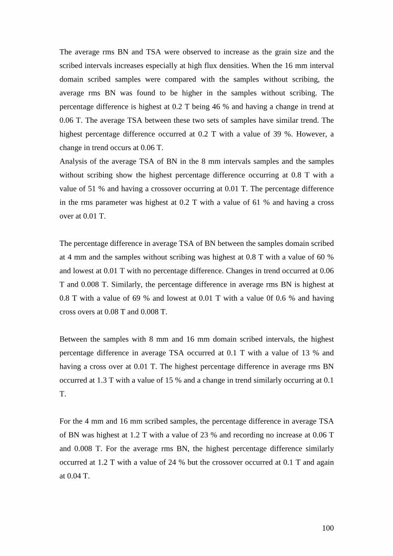
100

The average rms BN and TSA were observed to increase as the grain size and the

scribed intervals increases especially at high flux densities. When the 16 mm interval

domain scribed samples were compared with the samples without scribing, the

average rms BN was found to be higher in the samples without scribing. The

percentage difference is highest at 0.2 T being 46 % and having a change in trend at

0.06 T. The average TSA between these two sets of samples have similar trend. The

highest percentage difference occurred at 0.2 T with a value of 39 %. However, a

change in trend occurs at 0.06 T.

Analysis of the average TSA of BN in the 8 mm intervals samples and the samples

without scribing show the highest percentage difference occurring at 0.8 T with a

value of 51 % and having a crossover occurring at 0.01 T. The percentage difference

in the rms parameter was highest at 0.2 T with a value of 61 % and having a cross

over at 0.01 T.

The percentage difference in average TSA of BN between the samples domain scribed

at 4 mm and the samples without scribing was highest at 0.8 T with a value of 60 %

and lowest at 0.01 T with no percentage difference. Changes in trend occurred at 0.06

T and 0.008 T. Similarly, the percentage difference in average rms BN is highest at

0.8 T with a value of 69 % and lowest at 0.01 T with a value 0f 0.6 % and having

cross overs at 0.08 T and 0.008 T.

Between the samples with 8 mm and 16 mm domain scribed intervals, the highest

percentage difference in average TSA occurred at 0.1 T with a value of 13 % and

having a cross over at 0.01 T. The highest percentage difference in average rms BN

occurred at 1.3 T with a value of 15 % and a change in trend similarly occurring at 0.1

T.

For the 4 mm and 16 mm scribed samples, the percentage difference in average TSA

of BN was highest at 1.2 T with a value of 23 % and recording no increase at 0.06 T

and 0.008 T. For the average rms BN, the highest percentage difference similarly

occurred at 1.2 T with a value of 24 % but the crossover occurred at 0.1 T and again

at 0.04 T.

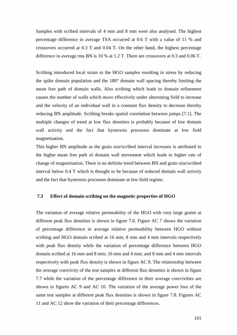
101

Samples with scribed intervals of 4 mm and 8 mm were also analysed. The highest

percentage difference in average TSA occurred at 0.6 T with a value of 11 % and

crossovers occurred at 0.3 T and 0.04 T. On the other hand, the highest percentage

difference in average rms BN is 10 % at 1.2 T. There are crossovers at 0.3 and 0.06 T.

Scribing introduced local strain to the HGO samples resulting in stress by reducing

the spike domain population and the 180° domain wall spacing thereby limiting the

mean free path of domain walls. Also scribing which leads to domain refinement

causes the number of walls which move effectively under alternating field to increase

and the velocity of an individual wall in a constant flux density to decrease thereby

reducing BN amplitude. Scribing breaks spatial correlation between jumps [7.1]. The

multiple changes of trend at low flux densities is probably because of low domain

wall activity and the fact that hysteresis processes dominate at low field

magnetisation.

This higher BN amplitude as the grain size/scribed interval increases is attributed to

the higher mean free path of domain wall movement which leads to higher rate of

change of magnetisation. There is no definite trend between BN and grain size/scribed

interval below 0.4 T which is thought to be because of reduced domain wall activity

and the fact that hysteresis processes dominate at low field regime.

7.3 Effect of domain scribing on the magnetic properties of HGO

The variation of average relative permeability of the HGO with very large grains at

different peak flux densities is shown in figure 7.6. Figure AC 7 shows the variation

of percentage difference in average relative permeability between HGO without

scribing and HGO domain scribed at 16 mm, 8 mm and 4 mm intervals respectively

with peak flux density while the variation of percentage difference between HGO

domain scribed at 16 mm and 8 mm; 16 mm and 4 mm; and 8 mm and 4 mm intervals

respectively with peak flux density is shown in figure AC 8. The relationship between

the average coercivity of the test samples at different flux densities is shown in figure

7.7 while the variation of the percentage difference in their average coercivities are

shown in figures AC 9 and AC 10. The variation of the average power loss of the

same test samples at different peak flux densities is shown in figure 7.8. Figures AC

11 and AC 12 show the variation of their percentage differences.

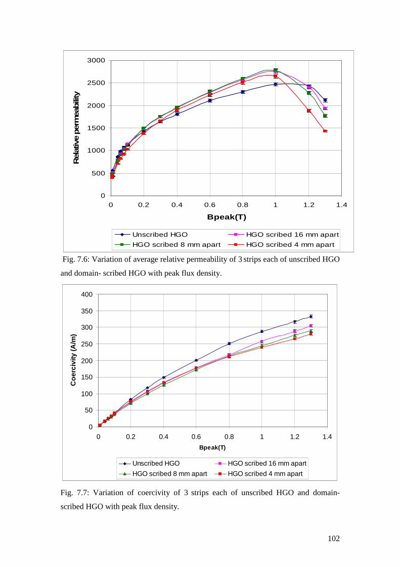
102

0

500

1000

1500

2000

2500

3000

0 0.2 0.4 0.6 0.8 1 1.2 1.4

Bpeak(T)

Rel

ativ

e per

mea

bili

ty

Unscribed HGO HGO scribed 16 mm apart

HGO scribed 8 mm apart HGO scribed 4 mm apart

Fig. 7.6: Variation of average relative permeability of 3 strips each of unscribed HGO

and domain- scribed HGO with peak flux density.

0

50

100

150

200

250

300

350

400

0 0.2 0.4 0.6 0.8 1 1.2 1.4

Bpeak(T)

Co

erci

vity

(A/m

)

Unscribed HGO HGO scribed 16 mm apart


Fig. 7.7: Variation of coercivity of 3 strips each of unscribed HGO and domain-

scribed HGO with peak flux density.

103

0

2

4

6

8

10

12

0 0.2 0.4 0.6 0.8 1 1.2 1.4

B(T)

Po

wer

loss

(W/k

g)

unscribed HGO HGO scribed 16 mm apart


Fig. 7.8: Variation of average power loss of 3 strips each of unscribed HGO and

domain- scribed HGO with peak flux density.

The percentage differences between the average relative permeability of test samples

at different flux densities are quantified and plotted in figures AC 7 and AC 8. For the

unscribed HGO, scribed HGO at 16 mm interval and the scribed HGO at 8 mm

interval, the average relative permeability follow almost a particular trend. It increases

with increasing grain size/scribe interval above 1.0 T. From 0.3 T -1.0 T, it decreases

with increasing grain size/scribe interval but the trend reverses from 0.008 T-0.1 T. At

0.2 T, the average relative permeability is highest in the 16 mm scribed samples and

lowest in the unscribed sample hence there is no definite trend here. 0.2 T is the

threshold between low and high flux densities. The trend at 0.3 T – 1.0 T is the

expected trend over the range of flux densities because very large grain samples

(unscribed HGO and the HGO scribed at 16 mm interval) have high power loss

because of large 180° domain wall spacing which lead to increase in anomalous loss.

It is at this range of flux densities that irreversible domain wall displacement

(maximum domain activity) takes place. The trend above 1.0 T and below 0.2 T is

probably because domain rotation and reversible domain wall motion take place

respectively in these regions with reduced domain activity. The average relative

permeability of the 4 mm scribed samples is the least of all flux densities compared to

Bpeak (T)

104

the other test samples. This is because the 4 mm scribed sample has a small domain

width (compared to the 8 mm scribed sample) with the resultant lower domain wall

activity.

The variation of the average coercivity and the average power loss of the test samples

at different peak flux densities are shown in figures 7.7 and 7.8 respectively and the

quantification of their percentage differences shown from figure AC 9 – AC 10 for

coercivity and figures AC 11 – AC 12 for power loss. For the unscribed HGO, scribed

HGO at 16 mm interval and scribed HGO at 8 mm interval, the coercivity and the

average power loss follow a particular trend at all flux densities. These magnetic

properties decrease with decreasing grain size/scribed interval. The reason is because

more domain refinement occurs as the scribed interval is reduced which decreases the

number of closure domains that contributes to increase in power loss and coercivity.

There is no particular trend in the coercivity and power loss of the 4 mm scribed HGO

sample in relation to the samples. This investigation shows that very large grains and

small grains (4 mm scribed interval) do not have good magnetic properties compared

to moderately large grains. This is because very large grain or large interval-scribed

sample will have very large domain width so domain walls will have freer path to

move thus generating more power loss in the process. The small interval-scribed

sample will have a lot of stress lines which impedes domain wall motion.

105

Reference to chapter 7

[7.1] T.W. Krause, L. Clapham, A. Pattantyus and D.L. Atherton, Investigation of the

stress dependent magnetic easy axis in steel using magnetic Barkhausen noise , J.

Appl. Phys. Vol. 79, No.8, pp. 4242-4252, 1996.

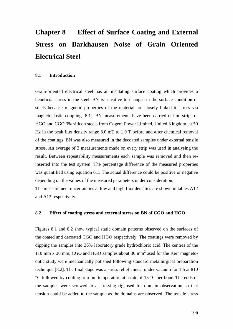
106

Chapter 8 Effect of Surface Coating and External

Stress on Barkhausen Noise of Grain Oriented

Electrical Steel

8.1 Introduction

Grain-oriented electrical steel has an insulating surface coating which provides a

beneficial stress in the steel. BN is sensitive to changes in the surface condition of

steels because magnetic properties of the material are closely linked to stress via

magnetoelastic coupling [8.1]. BN measurements have been carried out on strips of

HGO and CGO 3% silicon steels from Cogent Power Limited, United Kingdom, at 50

Hz in the peak flux density range 8.0 mT to 1.0 T before and after chemical removal

of the coatings. BN was also measured in the decoated samples under external tensile

stress. An average of 3 measurements made on every strip was used in analysing the

result. Between repeatability measurements each sample was removed and then re-

inserted into the test system. The percentage difference of the measured properties

was quantified using equation 6.1. The actual difference could be positive or negative

depending on the values of the measured parameters under consideration.

The measurement uncertainties at low and high flux densities are shown in tables A12

and A13 respectively.

8.2 Effect of coating stress and external stress on BN of CGO and HGO

Figures 8.1 and 8.2 show typical static domain patterns observed on the surfaces of

the coated and decoated CGO and HGO respectively. The coatings were removed by

dipping the samples into 36% laboratory grade hydrochloric acid. The centres of the

110 mm x 30 mm, CGO and HGO samples about 30 mm2 used for the Kerr magneto-

optic study were mechanically polished following standard metallurgical preparation

technique [8.2]. The final stage was a stress relief anneal under vacuum for 1 h at 810

°C followed by cooling to room temperature at a rate of 15° C per hour. The ends of

the samples were screwed to a stressing rig used for domain observation so that

tension could be added to the sample as the domains are observed. The tensile stress

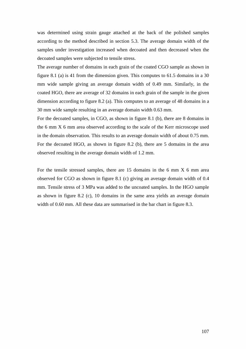
107

was determined using strain gauge attached at the back of the polished samples

according to the method described in section 5.3. The average domain width of the

samples under investigation increased when decoated and then decreased when the

decoated samples were subjected to tensile stress.

The average number of domains in each grain of the coated CGO sample as shown in

figure 8.1 (a) is 41 from the dimension given. This computes to 61.5 domains in a 30

mm wide sample giving an average domain width of 0.49 mm. Similarly, in the

coated HGO, there are average of 32 domains in each grain of the sample in the given

dimension according to figure 8.2 (a). This computes to an average of 48 domains in a

30 mm wide sample resulting in an average domain width 0.63 mm.

For the decoated samples, in CGO, as shown in figure 8.1 (b), there are 8 domains in

the 6 mm X 6 mm area observed according to the scale of the Kerr microscope used

in the domain observation. This results to an average domain width of about 0.75 mm.

For the decoated HGO, as shown in figure 8.2 (b), there are 5 domains in the area

observed resulting in the average domain width of 1.2 mm.

For the tensile stressed samples, there are 15 domains in the 6 mm X 6 mm area

observed for CGO as shown in figure 8.1 (c) giving an average domain width of 0.4

mm. Tensile stress of 3 MPa was added to the uncoated samples. In the HGO sample

as shown in figure 8.2 (c), 10 domains in the same area yields an average domain

width of 0.60 mm. All these data are summarised in the bar chart in figure 8.3.

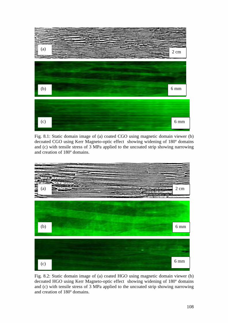
108

Fig. 8.1: Static domain image of (a) coated CGO using magnetic domain viewer (b) decoated CGO using Kerr Magneto-optic effect showing widening of 180º domains and (c) with tensile stress of 3 MPa applied to the uncoated strip showing narrowing and creation of 180º domains.

Fig. 8.2: Static domain image of (a) coated HGO using magnetic domain viewer (b) decoated HGO using Kerr Magneto-optic effect showing widening of 180º domains and (c) with tensile stress of 3 MPa applied to the uncoated strip showing narrowing and creation of 180º domains.

2 cm

2 cm

6 mm

6 mm

6 mm

6 mm

(a)

(b)

(c)

(a)

(b)

(c)

109

0

0.2

0.4

0.6

0.8

1

1.2

1.4

Coated CGO DecoatedCGO

Stressed CGO Coated HGO DecoatedHGO

Stressed HGO

Ave

rag

e d

om

ain

wid

th (m

m)

Fig. 8.3: Chart showing average domain width of coated, decoated and stressed-

decoated CGO and HGO samples under investigation.

Figures 8.4 and 8.5 show the corresponding variation of average rms BN with peak

flux density in the same strips of CGO and HGO respectively before and after coating

removal. The samples are the same as the domain viewed samples. The coating

removal causes the average rms BN to increase at any flux density in both materials.

The percentage increase in average rms BN arising from the coating removal in both

CGO and HGO are quantified and plotted in figure 8.6

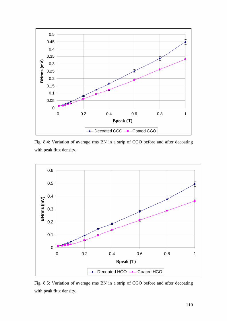
110

0

0.05

0.1

0.15

0.2

0.25

0.3

0.35

0.4

0.45

0.5

0 0.2 0.4 0.6 0.8 1

B(T)

BN

rms

(mV

)

Decoated CGO Coated CGO

Fig. 8.4: Variation of average rms BN in a strip of CGO before and after decoating

with peak flux density.

0

0.1

0.2

0.3

0.4

0.5

0.6

0 0.2 0.4 0.6 0.8 1

B(T)

BN

rms

(mV

)

Decoated HGO Coated HGO

Fig. 8.5: Variation of average rms BN in a strip of CGO before and after decoating


Bpeak (T)

Bpeak (T)

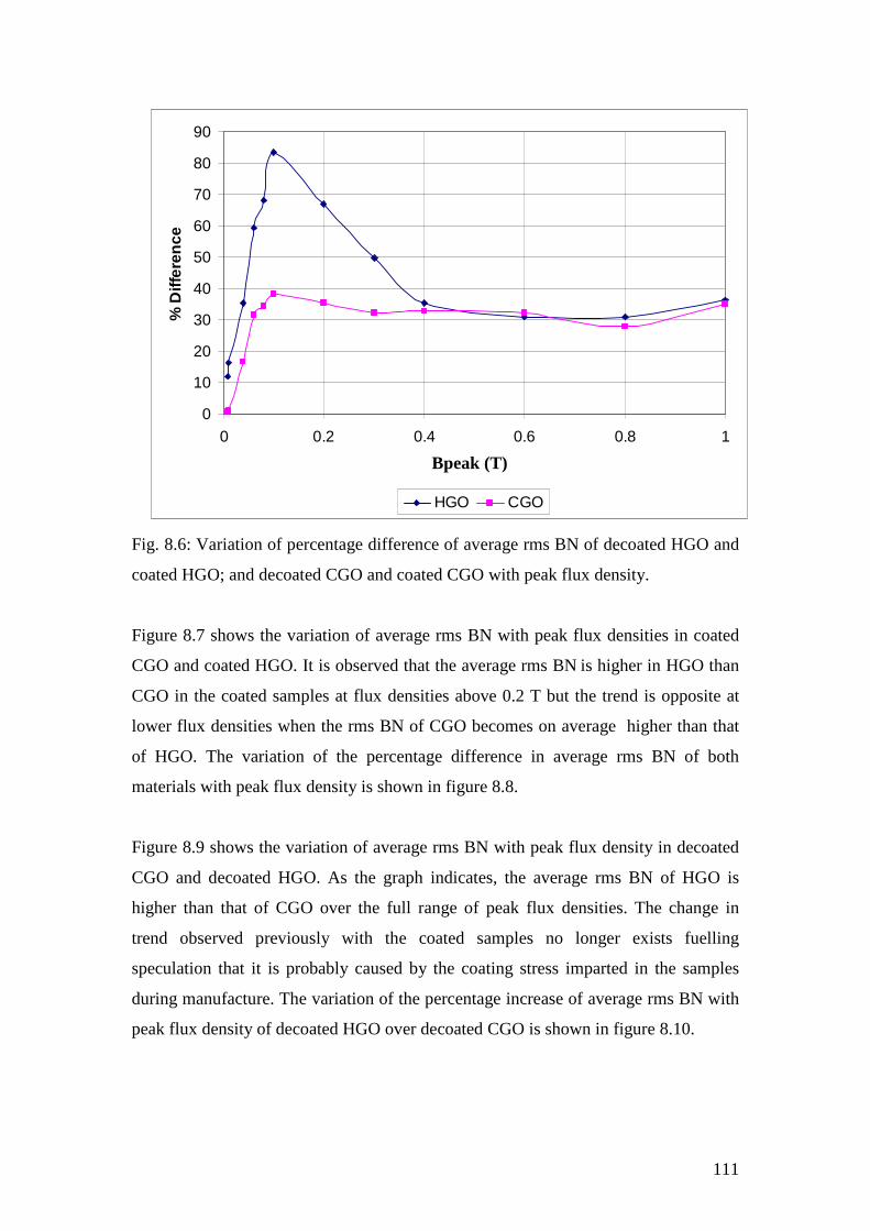
111

0

10

20

30

40

50

60

70

80

90

0 0.2 0.4 0.6 0.8 1

B(T)

% D

iffer

ence

HGO CGO

Fig. 8.6: Variation of percentage difference of average rms BN of decoated HGO and

coated HGO; and decoated CGO and coated CGO with peak flux density.

Figure 8.7 shows the variation of average rms BN with peak flux densities in coated

CGO and coated HGO. It is observed that the average rms BN is higher in HGO than

CGO in the coated samples at flux densities above 0.2 T but the trend is opposite at

lower flux densities when the rms BN of CGO becomes on average higher than that

of HGO. The variation of the percentage difference in average rms BN of both

materials with peak flux density is shown in figure 8.8.

Figure 8.9 shows the variation of average rms BN with peak flux density in decoated

CGO and decoated HGO. As the graph indicates, the average rms BN of HGO is

higher than that of CGO over the full range of peak flux densities. The change in

trend observed previously with the coated samples no longer exists fuelling

speculation that it is probably caused by the coating stress imparted in the samples

during manufacture. The variation of the percentage increase of average rms BN with

peak flux density of decoated HGO over decoated CGO is shown in figure 8.10.

Bpeak (T)

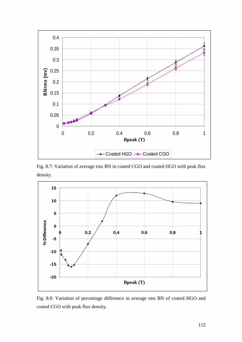
112

0

0.05

0.1

0.15

0.2

0.25

0.3

0.35

0.4

0 0.2 0.4 0.6 0.8 1

B(T)

BN

rms

(mv)

Coated HGO Coated CGO

Fig. 8.7: Variation of average rms BN in coated CGO and coated HGO with peak flux

density.

-20

-15

-10

-5

0

5

10

15

0 0.2 0.4 0.6 0.8 1

B(T)

% D

iffer

ence

Fig. 8.8: Variation of percentage difference in average rms BN of coated HGO and

coated CGO with peak flux density.

Bpeak (T)

Bpeak (T)

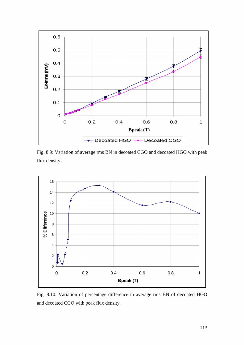
113

0

0.1

0.2

0.3

0.4

0.5

0.6

0 0.2 0.4 0.6 0.8 1

B(T)

BN

rms

(mV

)

Decoated HGO Decoated CGO

Fig. 8.9: Variation of average rms BN in decoated CGO and decoated HGO with peak

flux density.

0

2

4

6

8

10

12

14

16

0 0.2 0.4 0.6 0.8 1

Bpeak (T)

% D

iffer

ence

Fig. 8.10: Variation of percentage difference in average rms BN of decoated HGO

and decoated CGO with peak flux density.

Bpeak (T)

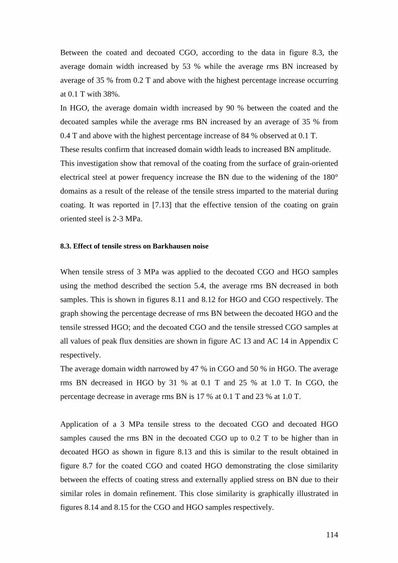
114

Between the coated and decoated CGO, according to the data in figure 8.3, the

average domain width increased by 53 % while the average rms BN increased by

average of 35 % from 0.2 T and above with the highest percentage increase occurring

at 0.1 T with 38%.

In HGO, the average domain width increased by 90 % between the coated and the

decoated samples while the average rms BN increased by an average of 35 % from

0.4 T and above with the highest percentage increase of 84 % observed at 0.1 T.

These results confirm that increased domain width leads to increased BN amplitude.

This investigation show that removal of the coating from the surface of grain-oriented

electrical steel at power frequency increase the BN due to the widening of the 180°

domains as a result of the release of the tensile stress imparted to the material during

coating. It was reported in [7.13] that the effective tension of the coating on grain

oriented steel is 2-3 MPa.

8.3. Effect of tensile stress on Barkhausen noise

When tensile stress of 3 MPa was applied to the decoated CGO and HGO samples

using the method described the section 5.4, the average rms BN decreased in both

samples. This is shown in figures 8.11 and 8.12 for HGO and CGO respectively. The

graph showing the percentage decrease of rms BN between the decoated HGO and the

tensile stressed HGO; and the decoated CGO and the tensile stressed CGO samples at

all values of peak flux densities are shown in figure AC 13 and AC 14 in Appendix C

respectively.

The average domain width narrowed by 47 % in CGO and 50 % in HGO. The average

rms BN decreased in HGO by 31 % at 0.1 T and 25 % at 1.0 T. In CGO, the

percentage decrease in average rms BN is 17 % at 0.1 T and 23 % at 1.0 T.

Application of a 3 MPa tensile stress to the decoated CGO and decoated HGO

samples caused the rms BN in the decoated CGO up to 0.2 T to be higher than in

decoated HGO as shown in figure 8.13 and this is similar to the result obtained in

figure 8.7 for the coated CGO and coated HGO demonstrating the close similarity

between the effects of coating stress and externally applied stress on BN due to their

similar roles in domain refinement. This close similarity is graphically illustrated in

figures 8.14 and 8.15 for the CGO and HGO samples respectively.

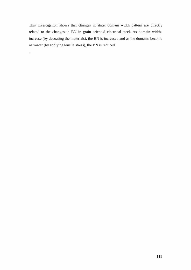
115

This investigation shows that changes in static domain width pattern are directly

related to the changes in BN in grain oriented electrical steel. As domain widths

increase (by decoating the materials), the BN is increased and as the domains become

narrower (by applying tensile stress), the BN is reduced.

.

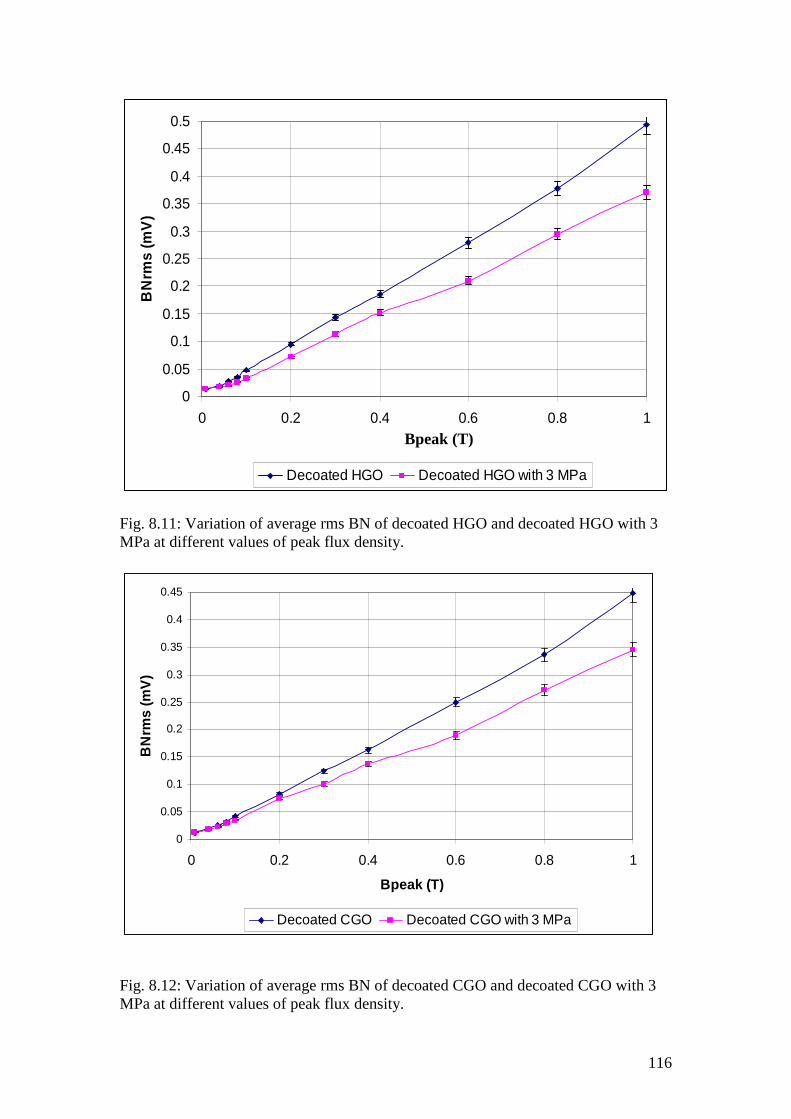
116

0

0.05

0.1

0.15

0.2

0.25

0.3

0.35

0.4

0.45

0.5

0 0.2 0.4 0.6 0.8 1B(T)

BN

rms

(mV

)

Decoated HGO Decoated HGO with 3 MPa

Fig. 8.11: Variation of average rms BN of decoated HGO and decoated HGO with 3 MPa at different values of peak flux density.

0

0.05

0.1

0.15

0.2

0.25

0.3

0.35

0.4

0.45

0 0.2 0.4 0.6 0.8 1

Bpeak (T)

BN

rms

(mV

)

Decoated CGO Decoated CGO with 3 MPa

Fig. 8.12: Variation of average rms BN of decoated CGO and decoated CGO with 3 MPa at different values of peak flux density.

Bpeak (T)

117

0

0.05

0.1

0.15

0.2

0.25

0.3

0.35

0.4

0.45

0 0.2 0.4 0.6 0.8 1B(T)

BN

rms

(mV

)

Decoated HGO with 3 MPa Decoated CGO with 3 MPa

Fig. 8.13: Variation of average rms BN in decoated CGO and HGO with tensile stress

of 3 MPa with at the various values of peak flux density.

Bpeak (T)

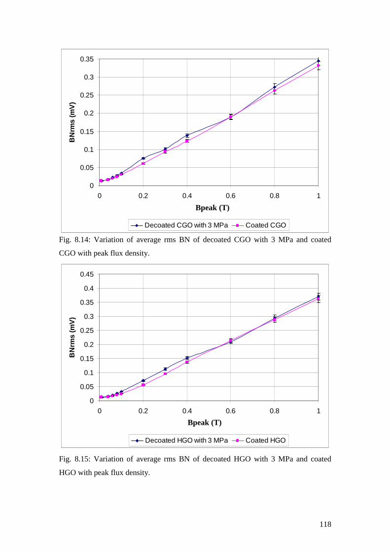
118

0

0.05

0.1

0.15

0.2

0.25

0.3

0.35

0 0.2 0.4 0.6 0.8 1

B(T)

BN

rms

(mV

)

Decoated CGO with 3 MPa Coated CGO

Fig. 8.14: Variation of average rms BN of decoated CGO with 3 MPa and coated

CGO with peak flux density.

0

0.05

0.1

0.15

0.2

0.25

0.3

0.35

0.4

0.45

0 0.2 0.4 0.6 0.8 1

B(T)

BN

rms

(mV

)

Decoated HGO with 3 MPa Coated HGO

Fig. 8.15: Variation of average rms BN of decoated HGO with 3 MPa and coated

HGO with peak flux density.

Bpeak (T)

Bpeak (T)

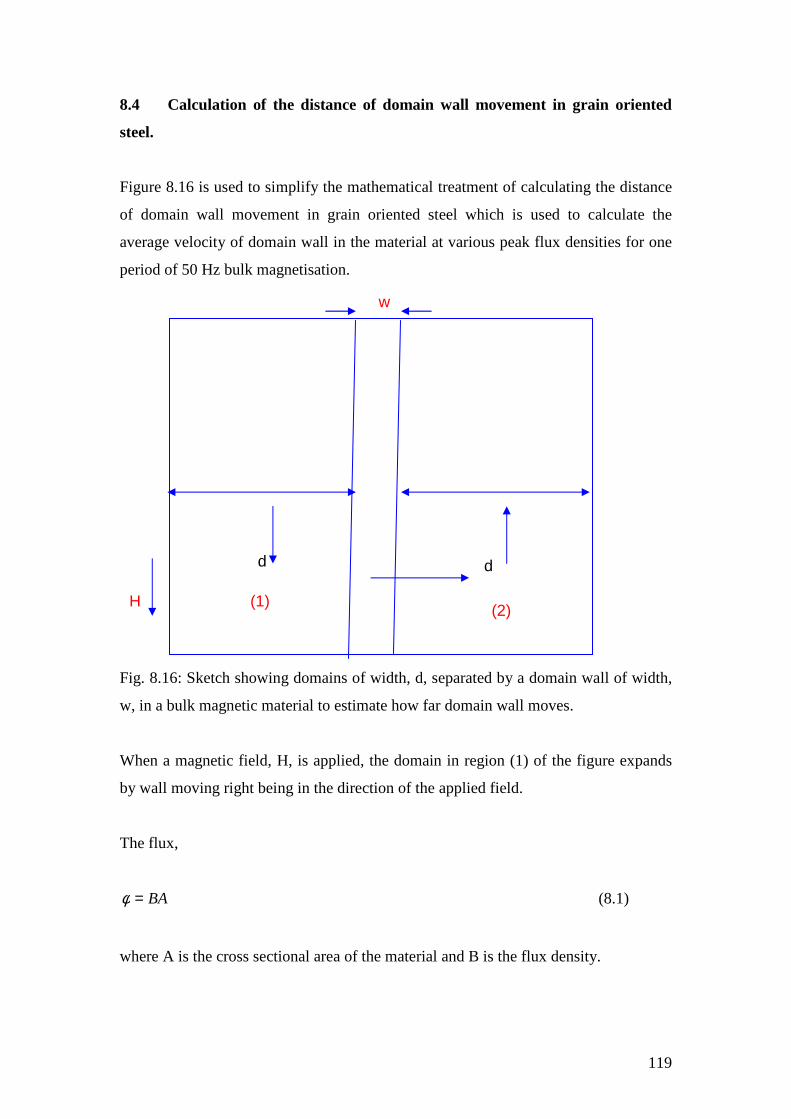
119

8.4 Calculation of the distance of domain wall movement in grain oriented

steel.

Figure 8.16 is used to simplify the mathematical treatment of calculating the distance

of domain wall movement in grain oriented steel which is used to calculate the

average velocity of domain wall in the material at various peak flux densities for one

period of 50 Hz bulk magnetisation.

Fig. 8.16: Sketch showing domains of width, d, separated by a domain wall of width,

w, in a bulk magnetic material to estimate how far domain wall moves.

When a magnetic field, H, is applied, the domain in region (1) of the figure expands

by wall moving right being in the direction of the applied field.

The flux,

BA=φ (8.1)

where A is the cross sectional area of the material and B is the flux density.

d d

w

H (1) (2)

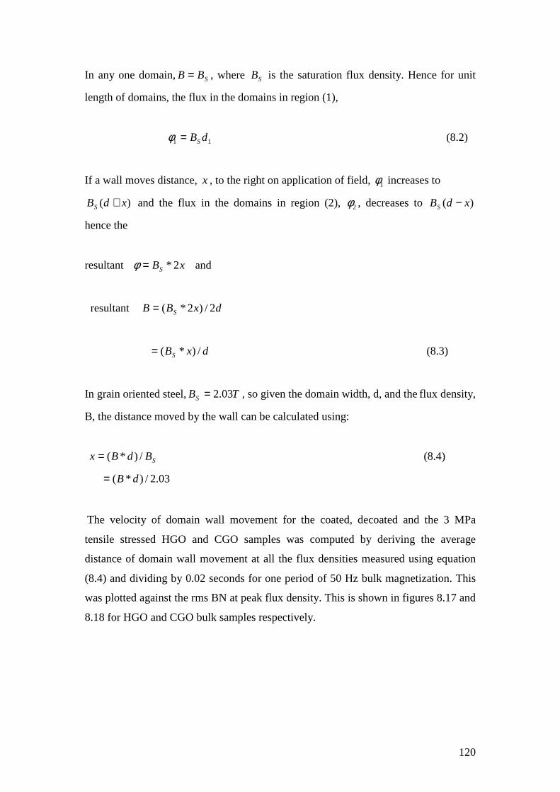
120

In any one domain, SBB = , where SB is the saturation flux density. Hence for unit

length of domains, the flux in the domains in region (1),

11 dBS=φ (8.2)

If a wall moves distance, x , to the right on application of field, 1φ increases to

)( xdBS + and the flux in the domains in region (2), 2φ , decreases to )( xdBS −

hence the

resultant xBS 2*=φ and

resultant dxBB S 2/)2*(=

dxBS /)*(= (8.3)

In grain oriented steel, TBS 03.2= , so given the domain width, d, and the flux density,

B, the distance moved by the wall can be calculated using:

SBdBx /)*(= (8.4)

03.2/)*( dB=

The velocity of domain wall movement for the coated, decoated and the 3 MPa

tensile stressed HGO and CGO samples was computed by deriving the average

distance of domain wall movement at all the flux densities measured using equation

(8.4) and dividing by 0.02 seconds for one period of 50 Hz bulk magnetization. This

was plotted against the rms BN at peak flux density. This is shown in figures 8.17 and

8.18 for HGO and CGO bulk samples respectively.

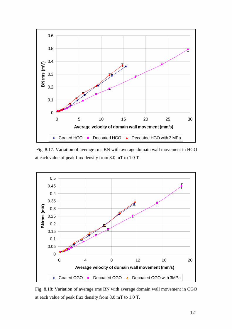
121

0

0.1

0.2

0.3

0.4

0.5

0.6

0 5 10 15 20 25 30

Average velocity of domain wall movement (mm/s)

BN

rms

(mV

)

Coated HGO Decoated HGO Decoated HGO with 3 MPa

Fig. 8.17: Variation of average rms BN with average domain wall movement in HGO

at each value of peak flux density from 8.0 mT to 1.0 T.

0

0.05

0.1

0.15

0.2

0.25

0.3

0.35

0.4

0.45

0.5

0 4 8 12 16 20

Average velocity of domain wall movement (mm/s)

BN

rms

(mV

)

Coated CGO Decoated CGO Decoated CGO with 3MPa

Fig. 8.18: Variation of average rms BN with average domain wall movement in CGO

at each value of peak flux density from 8.0 mT to 1.0 T.

122

The assumption in the above calculation is that domain wall motion does not vary

from grain to grain and sample to sample.

A significant correlation was found between the average velocities and changes in BN

at all the peak flux densities which demonstrates that the dominant factor responsible

for BN emission is the mean free path of domain wall movement and hence the width

of the predominant 180° domains in these materials.

Figure 8.19 shows the variation of average rms BN of decoated HGO, decoated HGO

with 2.3 MPa and decoated HGO with 3 MPa with peak flux density. It can be

observed that the average rms BN of the decoated sample is higher than that of the

tensile stressed samples at all the peak flux densities measured. When a tensile stress

of 2.3 MPa was applied, the average rms BN of the decoated HGO decreased by 30 %

at 0.1 T and 11 % at 1.0 T. When the amplitude of the tensile stress was increased to 3

MPa, the percentage decrease was 31 % at 0.1 T and 25 % at 1.0 T. Figure 8.22 shows

the variation of the percentage decrease in average rms BN at all measured flux

densities between the decoated HGO and the 2.3 MPa stressed HGO and also between

the decoated HGO and the 3 MPa stressed HGO. It can be observed that from 0.1 T

and below, the percentage difference between the average rms BN of the decoated

HGO and the 2.3 MPa stressed HGO on one hand and the decoated HGO and the 3.0

MPa stressed HGO on the other hand is almost the same. This suggests that in HGO,

at low flux densities, increase in tensile stress has very little effect on rms BN unlike

at high flux densities where the percentage difference is almost double. It can also be

observed that a change in trend occurred below 0.1 T between the tensile stressed

samples.

In CGO, as shown in figure 8.21, the average rms BN of the decoated sample is

higher than that of the tensile stressed samples at all flux densities except at 0.01 T

and 0.008 T where it became lower. When a tensile stress of 2.3 MPa was applied, the

average rms BN of the decoated HGO decreased by 18 % at 0.1 T and 12.5 % at 1.0

T. When the tensile stress was increased to 3 MPa, the average rms BN of the

decoated CGO decreased by 17 % at 0.1 T and 23 % at 1.0 T. Figure 8.22 shows the

variation of the percentage decrease between the average rms BN of the decoated

CGO and the tensile stressed CGO at all peak flux densities measured. It can be

observed that the amplitude of the average rms BN of the CGO with 2.3 MPa tensile

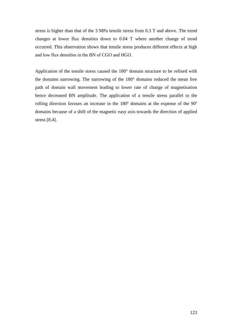
123

stress is higher than that of the 3 MPa tensile stress from 0.3 T and above. The trend

changes at lower flux densities down to 0.04 T where another change of trend

occurred. This observation shows that tensile stress produces different effects at high

and low flux densities in the BN of CGO and HGO.

Application of the tensile stress caused the 180° domain structure to be refined with

the domains narrowing. The narrowing of the 180° domains reduced the mean free

path of domain wall movement leading to lower rate of change of magnetisation

hence decreased BN amplitude. The application of a tensile stress parallel to the

rolling direction favours an increase in the 180º domains at the expense of the 90º

domains because of a shift of the magnetic easy axis towards the direction of applied

stress [8.4].

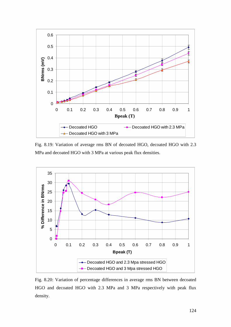
124

0

0.1

0.2

0.3

0.4

0.5

0.6

0 0.1 0.2 0.3 0.4 0.5 0.6 0.7 0.8 0.9 1

B(T)

BN

rms

(mV

)

Decoated HGO Decoated HGO with 2.3 MPa

Decoated HGO with 3 MPa

Fig. 8.19: Variation of average rms BN of decoated HGO, decoated HGO with 2.3

MPa and decoated HGO with 3 MPa at various peak flux densities.

0

5

10

15

20

25

30

35

0 0.1 0.2 0.3 0.4 0.5 0.6 0.7 0.8 0.9 1

Bpeak (T)

% D

iffer

ence

in B

Nrm

s

Decoated HGO and 2.3 Mpa stressed HGO

Decoated HGO and 3 Mpa stressed HGO

Fig. 8.20: Variation of percentage differences in average rms BN between decoated

HGO and decoated HGO with 2.3 MPa and 3 MPa respectively with peak flux

density.

Bpeak (T)

125

0

0.1

0.2

0.3

0.4

0.5

0 0.1 0.2 0.3 0.4 0.5 0.6 0.7 0.8 0.9 1

B(T)

BN

rms

(mV

)

Decoated CGO Decoated CGO with 2.3 MPa

Decoated CGO with 3 MPa

Fig. 8.21: Variation of average rms BN of decoated CGO, decoated CGO with 2.3

MPa and decoated CGO with 3 MPa at various peak flux densities.

-5

0

5

10

15

20

25

30

35

0 0.2 0.4 0.6 0.8 1

Bpeak (T)

% D

iffer

ence

in B

N r

ms

Decoated CGO and 2.3 MPa stressed CGO

Decoated CGO and 3 MPa stressed CGO

Fig. 8.22: Variation of percentage differences in average rms BN between decoated

CGO and decoated CGO with 2.3 MPa and 3 MPa respectively with peak flux

density.

Bpeak (T)

Bpeak (T)

126


[8.1] K. Gurruchaga, A. Martinez-de-Guerenu, M. Soto, and F. Arizti, “Magnetic

Barkhausen noise for characterization of recovery and recrystallization,” IEEE Trans.

Magn, vol. 46, no. 2, pp. 513-516, 2010.

[8.2] L. Bjerregaard, K. Geels, B. Ottesen and M. Ruckert, Metalog guide, Struers A/S,

Denmark, 1992.

[8.3] B. Fukuda, K. Satoh, T. Ichida, Y. Itoh, and H. Shimanaka, Effect of surface

coatings on domain structure in grain oriented 3% Si-Fe, IEEE Transactions on

Magnetics, Vol.17, No.6, pp. 2878-2880, 1981.

[8.4] T.W. Krause, L. Clapham, A. Pattantyus and D.L. Atherton, Investigation of the

stress dependent magnetic easy axis in steel using magnetic Barkhausen noise , J.

Appl. Phys. Vol. 79, No.8, pp. 4242-4252, 1996.

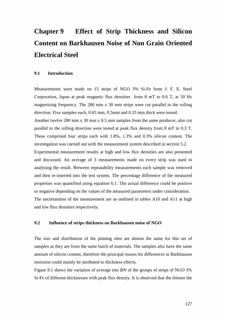
127

Chapter 9 Effect of Strip Thickness and Silicon

Content on Barkhausen Noise of Non Grain Oriented

Electrical Steel

9.1 Introduction

Measurements were made on 15 strips of NGO 3% Si-Fe from J. F. E. Steel

Corporation, Japan at peak magnetic flux densities from 8 mT to 0.6 T, at 50 Hz

magnetising frequency. The 280 mm x 30 mm strips were cut parallel to the rolling

direction. Five samples each, 0.65 mm, 0.5mm and 0.35 mm thick were tested.

Another twelve 280 mm x 30 mm x 0.5 mm samples from the same producer, also cut

parallel to the rolling direction were tested at peak flux density from 8 mT to 0.3 T.

These comprised four strips each with 1.8%, 1.3% and 0.3% silicon content. The

investigation was carried out with the measurement system described in section 5.2.

Experimental measurement results at high and low flux densities are also presented

and discussed. An average of 3 measurements made on every strip was used in

analysing the result. Between repeatability measurements each sample was removed

and then re-inserted into the test system. The percentage difference of the measured

properties was quantified using equation 6.1. The actual difference could be positive

or negative depending on the values of the measured parameters under consideration.

The uncertainties of the measurement are as outlined in tables A10 and A11 at high

and low flux densities respectively.

9.2 Influence of strips thickness on Barkhausen noise of NGO

The size and distribution of the pinning sites are almost the same for this set of

samples as they are from the same batch of materials. The samples also have the same

amount of silicon content, therefore the principal reason for differences in Barkhausen

emission could mainly be attributed to thickness effects.

Figure 9.1 shows the variation of average rms BN of the groups of strips of NGO 3%

Si-Fe of different thicknesses with peak flux density. It is observed that the thinner the

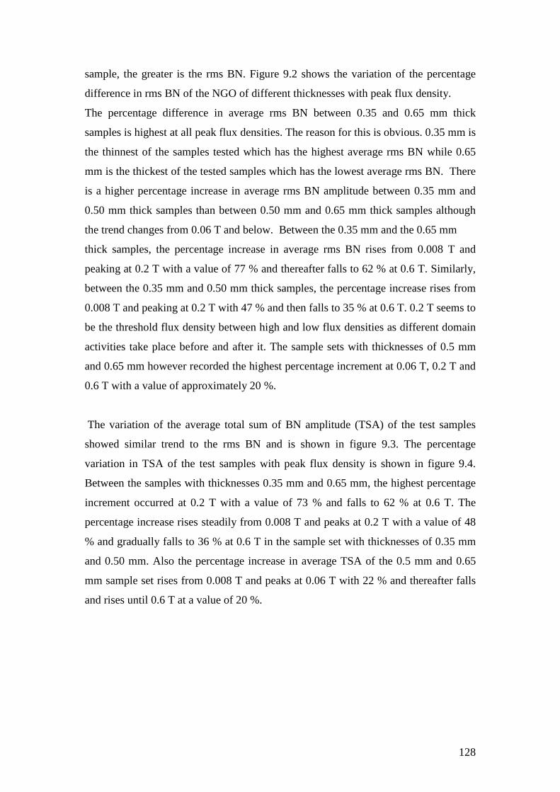
128

sample, the greater is the rms BN. Figure 9.2 shows the variation of the percentage

difference in rms BN of the NGO of different thicknesses with peak flux density.

The percentage difference in average rms BN between 0.35 and 0.65 mm thick

samples is highest at all peak flux densities. The reason for this is obvious. 0.35 mm is

the thinnest of the samples tested which has the highest average rms BN while 0.65

mm is the thickest of the tested samples which has the lowest average rms BN. There

is a higher percentage increase in average rms BN amplitude between 0.35 mm and

0.50 mm thick samples than between 0.50 mm and 0.65 mm thick samples although

the trend changes from 0.06 T and below. Between the 0.35 mm and the 0.65 mm

thick samples, the percentage increase in average rms BN rises from 0.008 T and

peaking at 0.2 T with a value of 77 % and thereafter falls to 62 % at 0.6 T. Similarly,

between the 0.35 mm and 0.50 mm thick samples, the percentage increase rises from

0.008 T and peaking at 0.2 T with 47 % and then falls to 35 % at 0.6 T. 0.2 T seems to

be the threshold flux density between high and low flux densities as different domain

activities take place before and after it. The sample sets with thicknesses of 0.5 mm

and 0.65 mm however recorded the highest percentage increment at 0.06 T, 0.2 T and

0.6 T with a value of approximately 20 %.

The variation of the average total sum of BN amplitude (TSA) of the test samples

showed similar trend to the rms BN and is shown in figure 9.3. The percentage

variation in TSA of the test samples with peak flux density is shown in figure 9.4.

Between the samples with thicknesses 0.35 mm and 0.65 mm, the highest percentage

increment occurred at 0.2 T with a value of 73 % and falls to 62 % at 0.6 T. The

percentage increase rises steadily from 0.008 T and peaks at 0.2 T with a value of 48

% and gradually falls to 36 % at 0.6 T in the sample set with thicknesses of 0.35 mm

and 0.50 mm. Also the percentage increase in average TSA of the 0.5 mm and 0.65

mm sample set rises from 0.008 T and peaks at 0.06 T with 22 % and thereafter falls

and rises until 0.6 T at a value of 20 %.

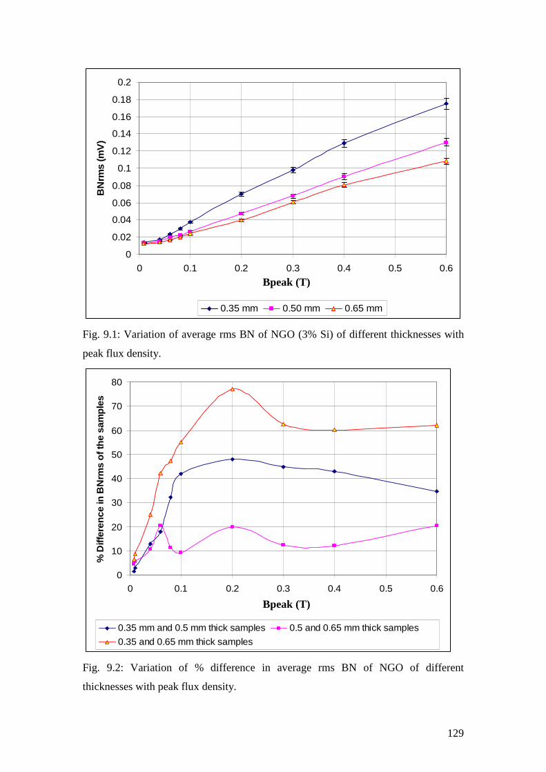
129

0

0.02

0.04

0.06

0.08

0.1

0.12

0.14

0.16

0.18

0.2

0 0.1 0.2 0.3 0.4 0.5 0.6

B(T)

BN

rms

(mV

)

0.35 mm 0.50 mm 0.65 mm

Fig. 9.1: Variation of average rms BN of NGO (3% Si) of different thicknesses with

peak flux density.

0

10

20

30

40

50

60

70

80

0 0.1 0.2 0.3 0.4 0.5 0.6

B(T)

% D

iffer

ence

in B

Nrm

s o

f th

e sa

mp

les

0.35 mm and 0.5 mm thick samples 0.5 and 0.65 mm thick samples

0.35 and 0.65 mm thick samples

Fig. 9.2: Variation of % difference in average rms BN of NGO of different

thicknesses with peak flux density.

Bpeak (T)

Bpeak (T)

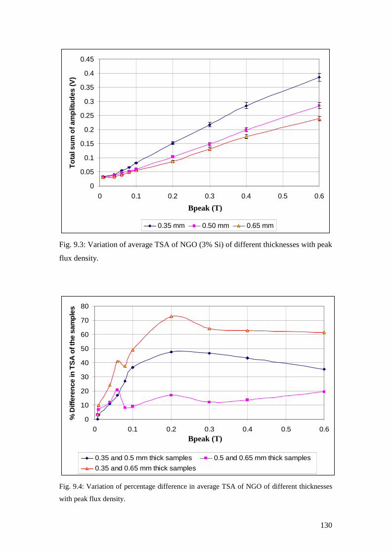
130

0

0.05

0.1

0.15

0.2

0.25

0.3

0.35

0.4

0.45

0 0.1 0.2 0.3 0.4 0.5 0.6

B(T)

To

tal s

um

of a

mp

litu

des

(V)

0.35 mm 0.50 mm 0.65 mm

Fig. 9.3: Variation of average TSA of NGO (3% Si) of different thicknesses with peak

flux density.

0

10

20

30

40

50

60

70

80

0 0.1 0.2 0.3 0.4 0.5 0.6

B(T)

% D

iffer

ence

in T

SA

of t

he

sam

ple

s

0.35 and 0.5 mm thick samples 0.5 and 0.65 mm thick samples

0.35 and 0.65 mm thick samples

Fig. 9.4: Variation of percentage difference in average TSA of NGO of different thicknesses


Bpeak (T)

Bpeak (T)

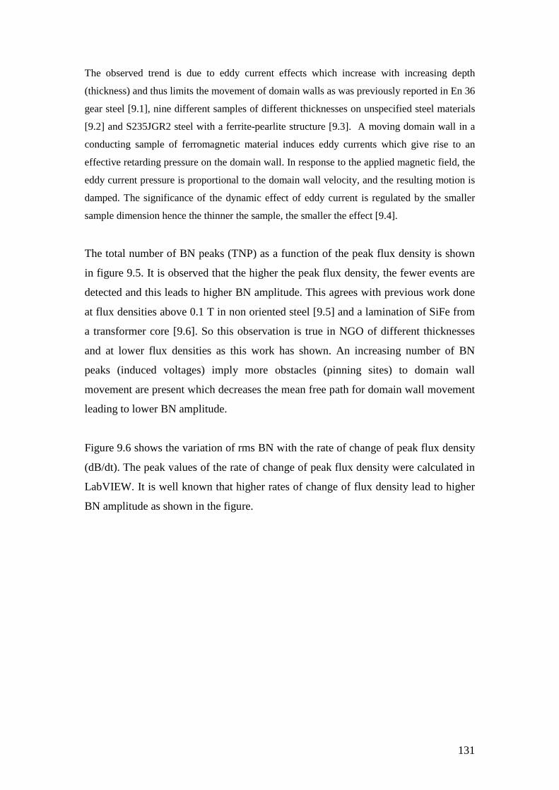
131

The observed trend is due to eddy current effects which increase with increasing depth

(thickness) and thus limits the movement of domain walls as was previously reported in En 36

gear steel [9.1], nine different samples of different thicknesses on unspecified steel materials

[9.2] and S235JGR2 steel with a ferrite-pearlite structure [9.3]. A moving domain wall in a

conducting sample of ferromagnetic material induces eddy currents which give rise to an

effective retarding pressure on the domain wall. In response to the applied magnetic field, the

eddy current pressure is proportional to the domain wall velocity, and the resulting motion is

damped. The significance of the dynamic effect of eddy current is regulated by the smaller

sample dimension hence the thinner the sample, the smaller the effect [9.4].

The total number of BN peaks (TNP) as a function of the peak flux density is shown

in figure 9.5. It is observed that the higher the peak flux density, the fewer events are

detected and this leads to higher BN amplitude. This agrees with previous work done

at flux densities above 0.1 T in non oriented steel [9.5] and a lamination of SiFe from

a transformer core [9.6]. So this observation is true in NGO of different thicknesses

and at lower flux densities as this work has shown. An increasing number of BN

peaks (induced voltages) imply more obstacles (pinning sites) to domain wall

movement are present which decreases the mean free path for domain wall movement

leading to lower BN amplitude.

Figure 9.6 shows the variation of rms BN with the rate of change of peak flux density

(dB/dt). The peak values of the rate of change of peak flux density were calculated in

LabVIEW. It is well known that higher rates of change of flux density lead to higher

BN amplitude as shown in the figure.

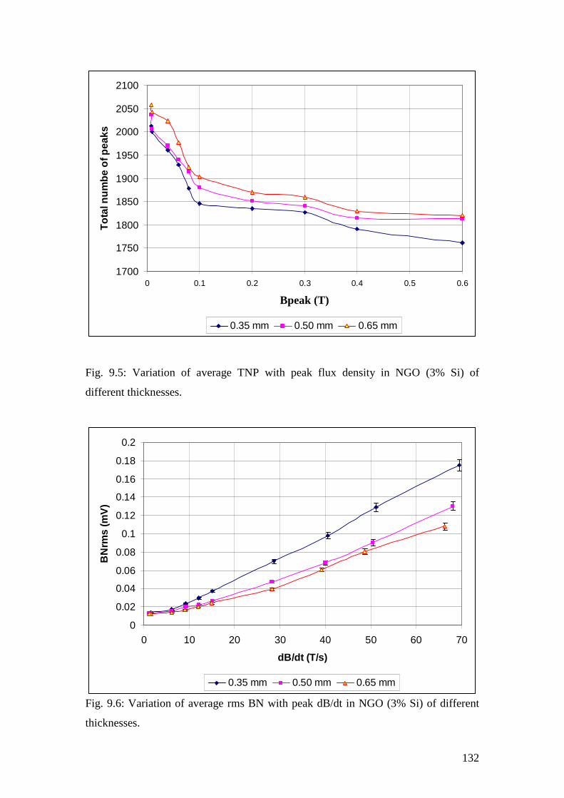
132

1700

1750

1800

1850

1900

1950

2000

2050

2100

0 0.1 0.2 0.3 0.4 0.5 0.6

B(T)

To

tal n

um

be

of p

eaks

0.35 mm 0.50 mm 0.65 mm

Fig. 9.5: Variation of average TNP with peak flux density in NGO (3% Si) of

different thicknesses.

0

0.02

0.04

0.06

0.08

0.1

0.12

0.14

0.16

0.18

0.2

0 10 20 30 40 50 60 70

dB/dt (T/s)

BN

rms

(mV

)

0.35 mm 0.50 mm 0.65 mm

Fig. 9.6: Variation of average rms BN with peak dB/dt in NGO (3% Si) of different

thicknesses.

Bpeak (T)

133

9.3 Influence of silicon content on Barkhausen noise of NGO

Figure 9.7 shows the variation of average rms BN with peak flux density in each of 4

strips of 0.5 mm thick NGO with different silicon contents. It is observed that the rms

BN increases as the silicon content increases. The variation of percentage difference

of the average rms BN of the test samples with peak flux density is shown in figure

9.8. The rms of BN increased by a much greater percentage between samples with

silicon contents of 1.3% and 1.8% than samples with silicon contents of 0.3% and

1.3% although there is a change of trend at 0.08 T and 0.06 T. The highest percentage

difference occurs between samples with silicon contents of 1.8% and 0.3% at all the

range of peak flux densities measured. The highest percentage increase in average rms

BN between the samples with silicon contents of 0.3 % and 1.8 % occurred at 0.3 T

with a value of over 155 %. Similarly, between the samples with silicon contents of

1.3 % and 1.8 %, the highest percentage increase occurred at 0.3 T at a value of 112

%. Between the samples with 0.3 % and 1.3 % silicon, the highest percentage increase

in average rms BN occurred at 0.08 T with 22 % and then falls and rises to 20 % at

0.3 T.

The average TSA of BN was also found to increase as the silicon content increases as

shown in figure 9.9. The percentage increases in TSA between the test samples as

shown in figure 9.10 has the same characteristics with the percentage increases in rms

BN of the test samples but there is no change of trend at lower flux densities. The

percentage increment in average TSA between the samples with silicon contents of

0.3 % and 1.8 % is higher than the percentage increment in all the other set of samples

measured. Between these test samples, the percentage difference in average TSA is

highest at 0.3 T at a value of 132 %. For the samples with 1.3 % and 1.8 % silicon

contents, the percentage difference maintained a steady increase from 0.04 T and

peaks at 0.3 T with 105 %. The highest percentage increase occurred 0.1 T with a

value of 22 % and fall to 15 % at 0.3 T between the samples with silicon contents of

0.3 % and 1.3 %.

These observations are also due to BN signals being attenuated by eddy current

shielding effects. Higher silicon content causes the eddy current shielding effect to be

reduced which decreases the retarding eddy current pressure on the domain walls

resulting in the higher BN amplitude. Eddy-current losses are inevitable in conducting

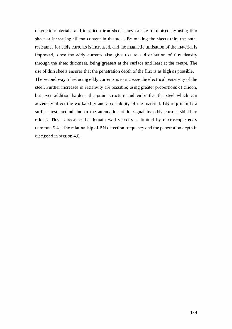
134

magnetic materials, and in silicon iron sheets they can be minimised by using thin

sheet or increasing silicon content in the steel. By making the sheets thin, the path-

resistance for eddy currents is increased, and the magnetic utilisation of the material is

improved, since the eddy currents also give rise to a distribution of flux density

through the sheet thickness, being greatest at the surface and least at the centre. The

use of thin sheets ensures that the penetration depth of the flux is as high as possible.

The second way of reducing eddy currents is to increase the electrical resistivity of the

steel. Further increases in resistivity are possible; using greater proportions of silicon,

but over addition hardens the grain structure and embrittles the steel which can

adversely affect the workability and applicability of the material. BN is primarily a

surface test method due to the attenuation of its signal by eddy current shielding

effects. This is because the domain wall velocity is limited by microscopic eddy

currents [9.4]. The relationship of BN detection frequency and the penetration depth is

discussed in section 4.6.

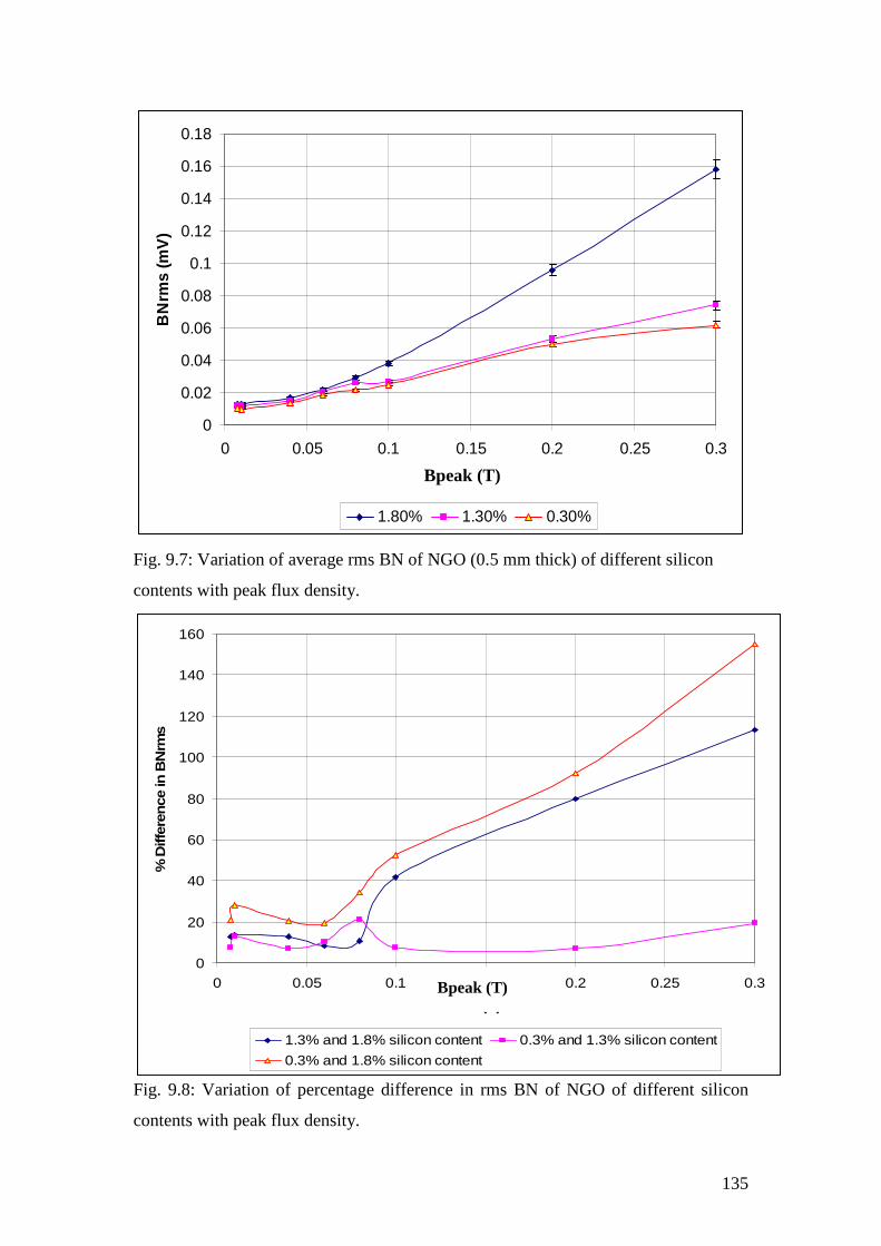
135

0

0.02

0.04

0.06

0.08

0.1

0.12

0.14

0.16

0.18

0 0.05 0.1 0.15 0.2 0.25 0.3

B(T)

BN

rms

(mV

)

1.80% 1.30% 0.30%

Fig. 9.7: Variation of average rms BN of NGO (0.5 mm thick) of different silicon

contents with peak flux density.

0

20

40

60

80

100

120

140

160

0 0.05 0.1 0.15 0.2 0.25 0.3

B(T)

% D

iffer

ence

in B

Nrm

s

1.3% and 1.8% silicon content 0.3% and 1.3% silicon content

0.3% and 1.8% silicon content

Fig. 9.8: Variation of percentage difference in rms BN of NGO of different silicon


Bpeak (T)

Bpeak (T)

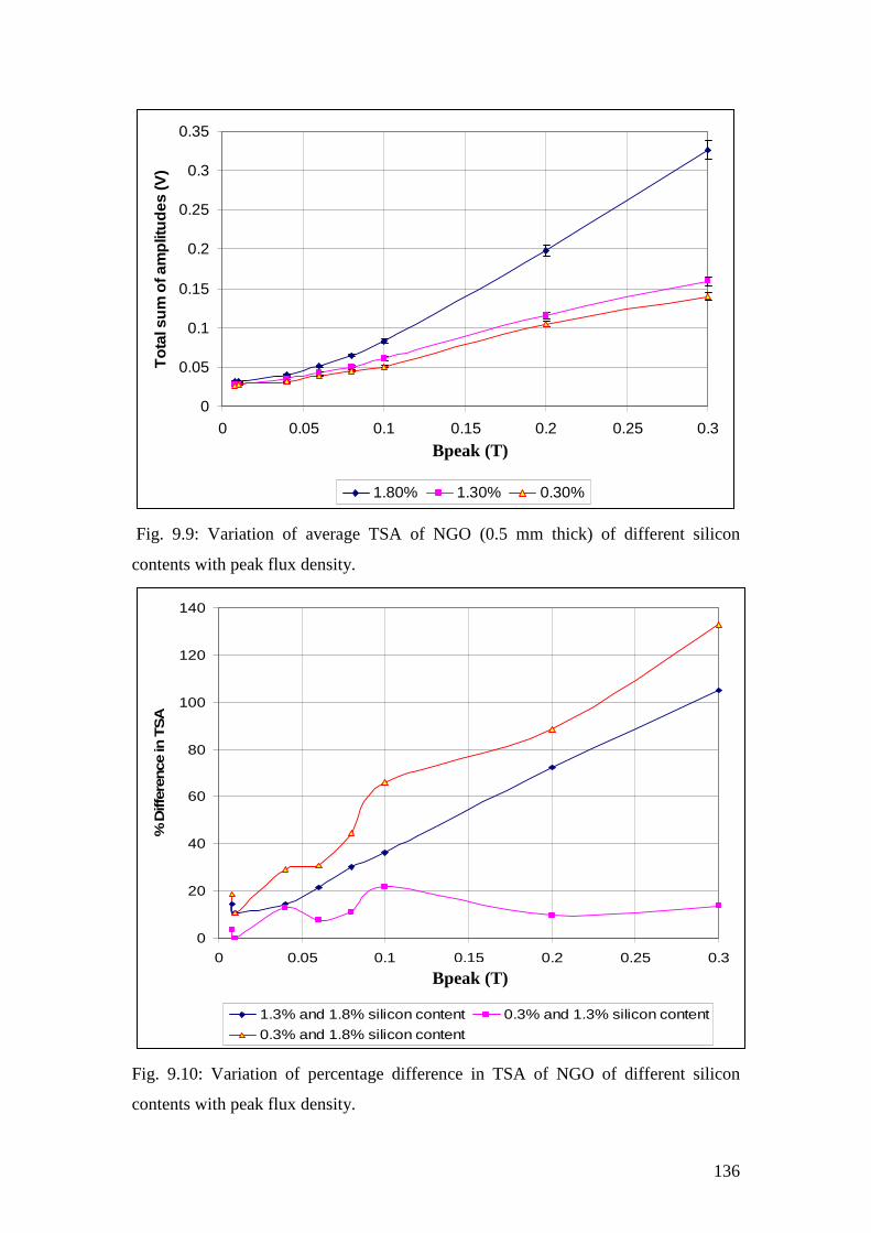
136

0

0.05

0.1

0.15

0.2

0.25

0.3

0.35

0 0.05 0.1 0.15 0.2 0.25 0.3

B(T)

To

tal s

um

of a

mp

litu

des

(V)

1.80% 1.30% 0.30%

Fig. 9.9: Variation of average TSA of NGO (0.5 mm thick) of different silicon


0

20

40

60

80

100

120

140

0 0.05 0.1 0.15 0.2 0.25 0.3

B(T)

% D

iffer

ence

in T

SA

1.3% and 1.8% silicon content 0.3% and 1.3% silicon content

0.3% and 1.8% silicon content

Fig. 9.10: Variation of percentage difference in TSA of NGO of different silicon


Bpeak (T)

Bpeak (T)

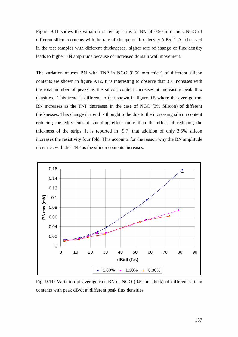
137

Figure 9.11 shows the variation of average rms of BN of 0.50 mm thick NGO of

different silicon contents with the rate of change of flux density (dB/dt). As observed

in the test samples with different thicknesses, higher rate of change of flux density

leads to higher BN amplitude because of increased domain wall movement.

The variation of rms BN with TNP in NGO (0.50 mm thick) of different silicon

contents are shown in figure 9.12. It is interesting to observe that BN increases with

the total number of peaks as the silicon content increases at increasing peak flux

densities. This trend is different to that shown in figure 9.5 where the average rms

BN increases as the TNP decreases in the case of NGO (3% Silicon) of different

thicknesses. This change in trend is thought to be due to the increasing silicon content

reducing the eddy current shielding effect more than the effect of reducing the

thickness of the strips. It is reported in [9.7] that addition of only 3.5% silicon

increases the resistivity four fold. This accounts for the reason why the BN amplitude

increases with the TNP as the silicon contents increases.

0

0.02

0.04

0.06

0.08

0.1

0.12

0.14

0.16

0 10 20 30 40 50 60 70 80 90

dB/dt (T/s)

BN

rms

(mV

)

1.80% 1.30% 0.30%

Fig. 9.11: Variation of average rms BN of NGO (0.5 mm thick) of different silicon

contents with peak dB/dt at different peak flux densities.

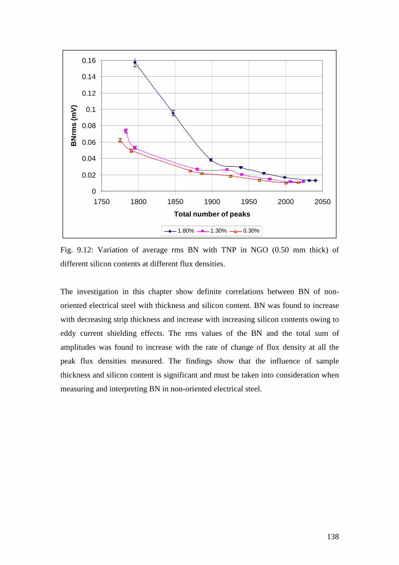
138

0

0.02

0.04

0.06

0.08

0.1

0.12

0.14

0.16

1750 1800 1850 1900 1950 2000 2050

Total number of peaks

BN

rms

(mV

)

1.80% 1.30% 0.30%

Fig. 9.12: Variation of average rms BN with TNP in NGO (0.50 mm thick) of

different silicon contents at different flux densities.

The investigation in this chapter show definite correlations between BN of non-

oriented electrical steel with thickness and silicon content. BN was found to increase

with decreasing strip thickness and increase with increasing silicon contents owing to

eddy current shielding effects. The rms values of the BN and the total sum of

amplitudes was found to increase with the rate of change of flux density at all the

peak flux densities measured. The findings show that the influence of sample

thickness and silicon content is significant and must be taken into consideration when

measuring and interpreting BN in non-oriented electrical steel.

139


[9.1] J W. Wilson, G. Y. Tian, V. Moorthy and B. A. Shaw, Magneto-acoustic

emission and magnetic Barkhausen emission for case depth measurement in En36

gear steel, IEEE Transactions on Magnetics, Vol. 45, No.1, pp. 177-183, 2009.

[9.2] D. Strand, Parameters and depth of penetration of Barkhausen noise analysis,

United States Army Research Laboratory, ARL-TR-5159, pp. 1-11, 2010.

[9.3] T. Garstka, The influence of product thickness on the measurements by

Barkhausen noise method, Journal of Achievements in Materials and Manufacturing

Engineering, Vol. 27, issue 1, pp. 47-50, 2008.

[9.4] F. Colaiori, G. Durin, and S. Zapperil, Eddy current damping of a moving

domain wall: Beyond the quasistatic approximation, Physical Review B 76, 224416,

pp. 1-7, 2007.

[9.5] M. Komatsubara, J. L. Porteseil, Influence of grain size and strain on

Barkhausen noise power on non-oriented silicon steel, IEEE Transactions on

Magnetics, Vol. 23, issue 5, pp. 3506-3508, 1987.

[9.6] S. White, T. Krause, and L. Clapham, Quantitative analysis of surface

Barkhausen noise measurements, Review of Quantitative Non-destructive

Evaluation, Vol. 27, pp. 445-452, 2008.

[9.7] F Brailsford, Physical principles of Magnetism, Van Nostrand, London, 1966.

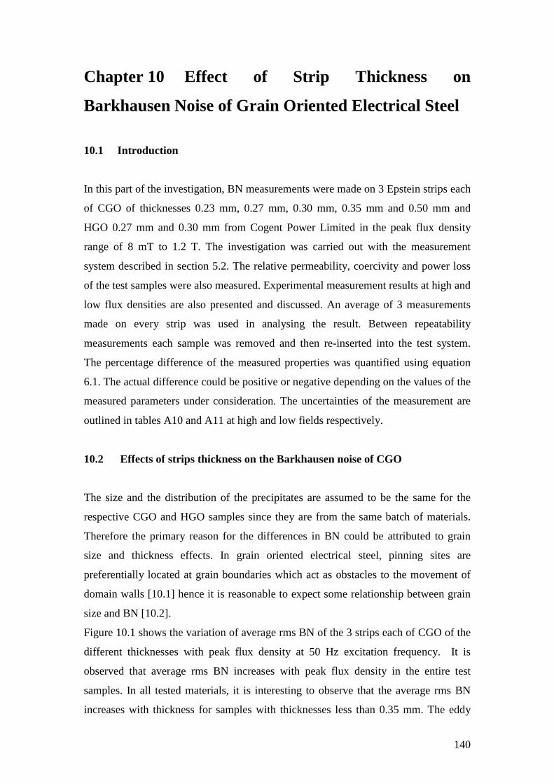
140

Chapter 10 Effect of Strip Thickness on

Barkhausen Noise of Grain Oriented Electrical Steel

10.1 Introduction

In this part of the investigation, BN measurements were made on 3 Epstein strips each

of CGO of thicknesses 0.23 mm, 0.27 mm, 0.30 mm, 0.35 mm and 0.50 mm and

HGO 0.27 mm and 0.30 mm from Cogent Power Limited in the peak flux density

range of 8 mT to 1.2 T. The investigation was carried out with the measurement

system described in section 5.2. The relative permeability, coercivity and power loss

of the test samples were also measured. Experimental measurement results at high and

low flux densities are also presented and discussed. An average of 3 measurements

made on every strip was used in analysing the result. Between repeatability

measurements each sample was removed and then re-inserted into the test system.

The percentage difference of the measured properties was quantified using equation

6.1. The actual difference could be positive or negative depending on the values of the

measured parameters under consideration. The uncertainties of the measurement are

outlined in tables A10 and A11 at high and low fields respectively.

10.2 Effects of strips thickness on the Barkhausen noise of CGO

The size and the distribution of the precipitates are assumed to be the same for the

respective CGO and HGO samples since they are from the same batch of materials.

Therefore the primary reason for the differences in BN could be attributed to grain

size and thickness effects. In grain oriented electrical steel, pinning sites are

preferentially located at grain boundaries which act as obstacles to the movement of

domain walls [10.1] hence it is reasonable to expect some relationship between grain

size and BN [10.2].

Figure 10.1 shows the variation of average rms BN of the 3 strips each of CGO of the

different thicknesses with peak flux density at 50 Hz excitation frequency. It is

observed that average rms BN increases with peak flux density in the entire test

samples. In all tested materials, it is interesting to observe that the average rms BN

increases with thickness for samples with thicknesses less than 0.35 mm. The eddy

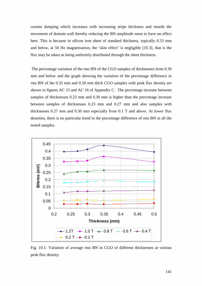
141

current damping which increases with increasing strips thickness and retards the

movement of domain wall thereby reducing the BN amplitude seem to have no effect

here. This is because in silicon iron sheet of standard thickness, typically 0.33 mm

and below, at 50 Hz magnetisation, the ‘skin effect’ is negligible [10.3], that is the

flux may be taken as being uniformly distributed through the sheet thickness.

The percentage variation of the rms BN of the CGO samples of thicknesses from 0.30

mm and below and the graph showing the variation of the percentage difference in

rms BN of the 0.35 mm and 0.50 mm thick CGO samples with peak flux density are

shown in figures AC 15 and AC 16 of Appendix C. The percentage increase between

samples of thicknesses 0.23 mm and 0.30 mm is higher than the percentage increase

between samples of thicknesses 0.23 mm and 0.27 mm and also samples with

thicknesses 0.27 mm and 0.30 mm especially from 0.1 T and above. At lower flux

densities, there is no particular trend in the percentage difference of rms BN in all the

tested samples.

0

0.05

0.1

0.15

0.2

0.25

0.3

0.35

0.4

0.45

0.2 0.25 0.3 0.35 0.4 0.45 0.5

Thickness (mm)

BN

rms

(mV

)

1.2T 1.0 T 0.8 T 0.6 T 0.4 T

0.2 T 0.1 T

Fig. 10.1: Variation of average rms BN in CGO of different thicknesses at various

peak flux density.

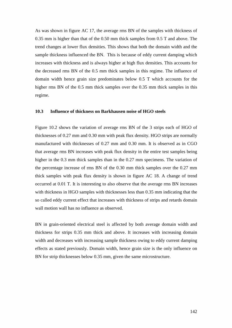
142

As was shown in figure AC 17, the average rms BN of the samples with thickness of

0.35 mm is higher than that of the 0.50 mm thick samples from 0.5 T and above. The

trend changes at lower flux densities. This shows that both the domain width and the

sample thickness influenced the BN. This is because of eddy current damping which

increases with thickness and is always higher at high flux densities. This accounts for

the decreased rms BN of the 0.5 mm thick samples in this regime. The influence of

domain width hence grain size predominates below 0.5 T which accounts for the

higher rms BN of the 0.5 mm thick samples over the 0.35 mm thick samples in this

regime.

10.3 Influence of thickness on Barkhausen noise of HGO steels

Figure 10.2 shows the variation of average rms BN of the 3 strips each of HGO of

thicknesses of 0.27 mm and 0.30 mm with peak flux density. HGO strips are normally

manufactured with thicknesses of 0.27 mm and 0.30 mm. It is observed as in CGO

that average rms BN increases with peak flux density in the entire test samples being

higher in the 0.3 mm thick samples than in the 0.27 mm specimens. The variation of

the percentage increase of rms BN of the 0.30 mm thick samples over the 0.27 mm

thick samples with peak flux density is shown in figure AC 18. A change of trend

occurred at 0.01 T. It is interesting to also observe that the average rms BN increases

with thickness in HGO samples with thicknesses less than 0.35 mm indicating that the

so called eddy current effect that increases with thickness of strips and retards domain

wall motion wall has no influence as observed.

BN in grain-oriented electrical steel is affected by both average domain width and

thickness for strips 0.35 mm thick and above. It increases with increasing domain

width and decreases with increasing sample thickness owing to eddy current damping

effects as stated previously. Domain width, hence grain size is the only influence on

BN for strip thicknesses below 0.35 mm, given the same microstructure.

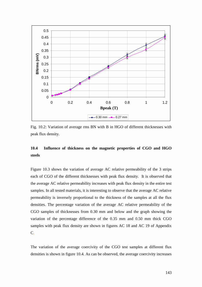
143

0

0.05

0.1

0.15

0.2

0.25

0.3

0.35

0.4

0.45

0.5

0 0.2 0.4 0.6 0.8 1 1.2

B(T)

BN

rms

(mV

)

0.30 mm 0.27 mm

Fig. 10.2: Variation of average rms BN with B in HGO of different thicknesses with

peak flux density.

10.4 Influence of thickness on the magnetic properties of CGO and HGO

steels

Figure 10.3 shows the variation of average AC relative permeability of the 3 strips

each of CGO of the different thicknesses with peak flux density. It is observed that

the average AC relative permeability increases with peak flux density in the entire test

samples. In all tested materials, it is interesting to observe that the average AC relative

permeability is inversely proportional to the thickness of the samples at all the flux

densities. The percentage variation of the average AC relative permeability of the

CGO samples of thicknesses from 0.30 mm and below and the graph showing the

variation of the percentage difference of the 0.35 mm and 0.50 mm thick CGO

samples with peak flux density are shown in figures AC 18 and AC 19 of Appendix

C.

The variation of the average coercivity of the CGO test samples at different flux

densities is shown in figure 10.4. As can be observed, the average coercivity increases

Bpeak (T)

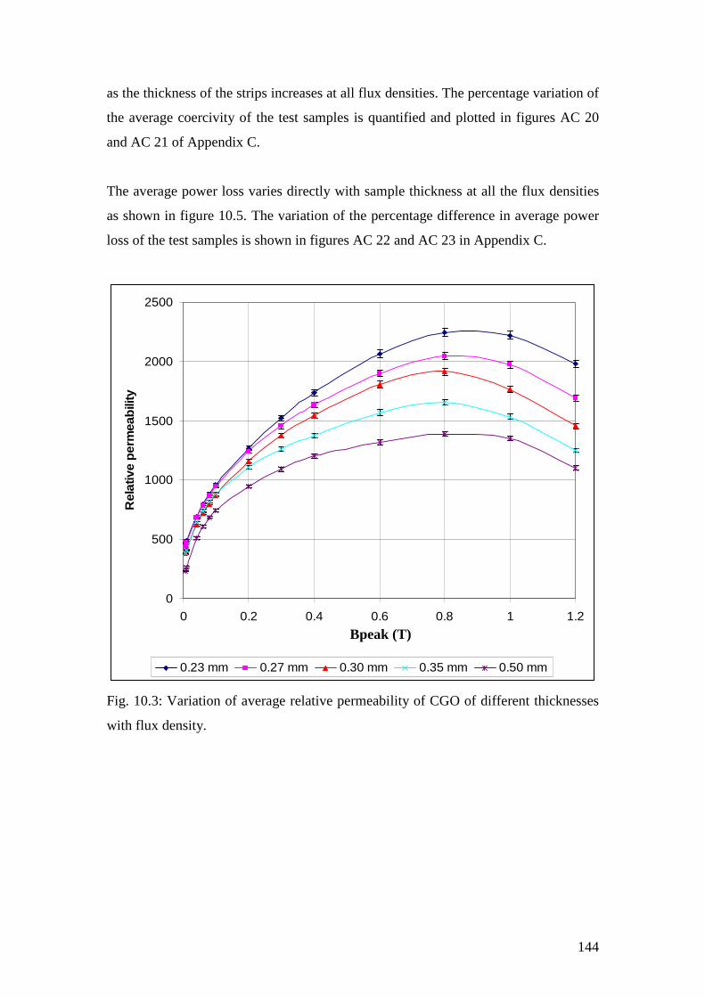
144

as the thickness of the strips increases at all flux densities. The percentage variation of

the average coercivity of the test samples is quantified and plotted in figures AC 20

and AC 21 of Appendix C.

The average power loss varies directly with sample thickness at all the flux densities

as shown in figure 10.5. The variation of the percentage difference in average power

loss of the test samples is shown in figures AC 22 and AC 23 in Appendix C.

0

500

1000

1500

2000

2500

0 0.2 0.4 0.6 0.8 1 1.2

B(T)

Rel

ativ

e p

erm

eab

ility

0.23 mm 0.27 mm 0.30 mm 0.35 mm 0.50 mm

Fig. 10.3: Variation of average relative permeability of CGO of different thicknesses

with flux density.

Bpeak (T)

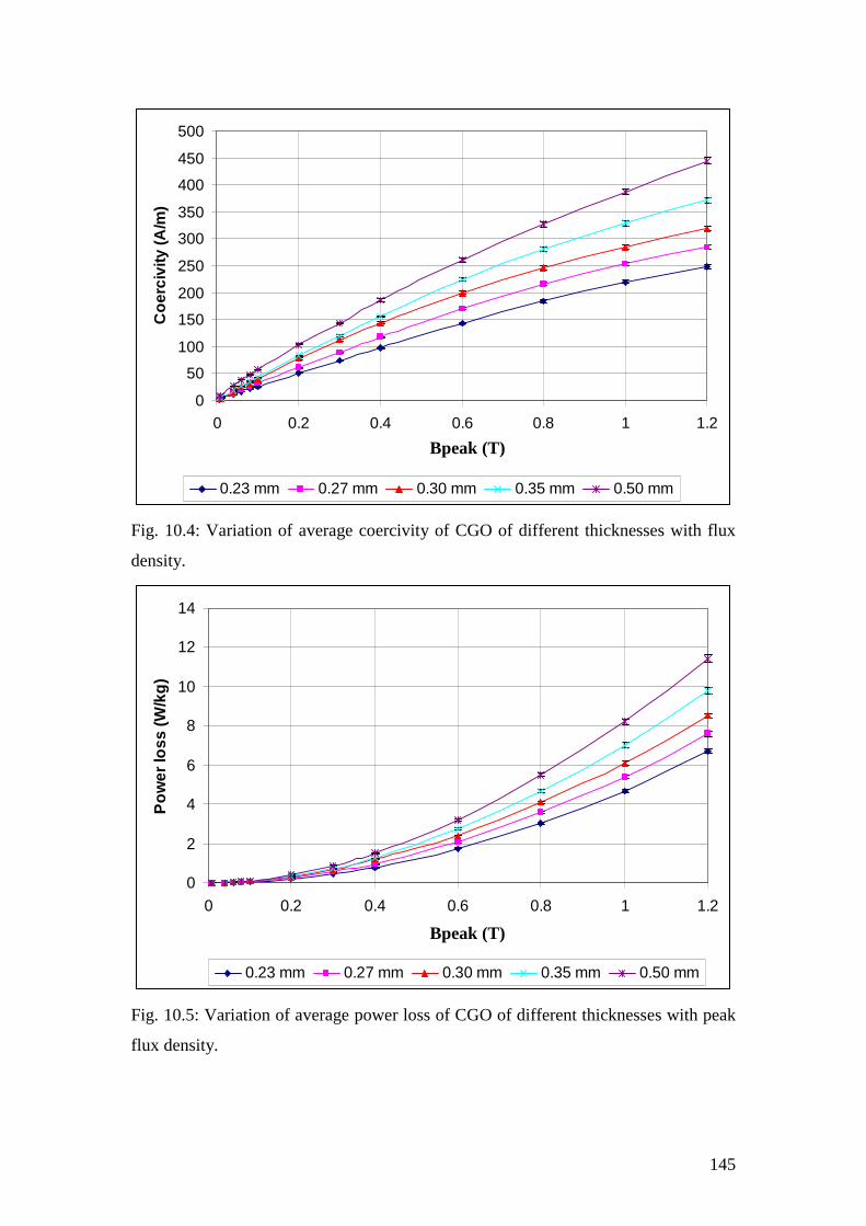
145

0

50

100

150

200

250

300

350

400

450

500

0 0.2 0.4 0.6 0.8 1 1.2

B(T)

Co

erci

vity

(A/m

)

0.23 mm 0.27 mm 0.30 mm 0.35 mm 0.50 mm

Fig. 10.4: Variation of average coercivity of CGO of different thicknesses with flux

density.

0

2

4

6

8

10

12

14

0 0.2 0.4 0.6 0.8 1 1.2

B(T)

Po

wer

loss

(W/k

g)

0.23 mm 0.27 mm 0.30 mm 0.35 mm 0.50 mm

Fig. 10.5: Variation of average power loss of CGO of different thicknesses with peak

flux density.

Bpeak (T)

Bpeak (T)

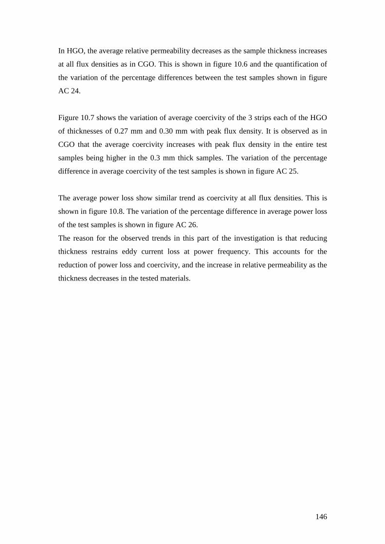
146

In HGO, the average relative permeability decreases as the sample thickness increases

at all flux densities as in CGO. This is shown in figure 10.6 and the quantification of

the variation of the percentage differences between the test samples shown in figure

AC 24.

Figure 10.7 shows the variation of average coercivity of the 3 strips each of the HGO

of thicknesses of 0.27 mm and 0.30 mm with peak flux density. It is observed as in

CGO that the average coercivity increases with peak flux density in the entire test

samples being higher in the 0.3 mm thick samples. The variation of the percentage

difference in average coercivity of the test samples is shown in figure AC 25.

The average power loss show similar trend as coercivity at all flux densities. This is

shown in figure 10.8. The variation of the percentage difference in average power loss

of the test samples is shown in figure AC 26.

The reason for the observed trends in this part of the investigation is that reducing

thickness restrains eddy current loss at power frequency. This accounts for the

reduction of power loss and coercivity, and the increase in relative permeability as the

thickness decreases in the tested materials.

147

0

500

1000

1500

2000

2500

3000

0 0.2 0.4 0.6 0.8 1 1.2

B(T)

Rel

ativ

e p

erm

eab

ility

0.27 mm 0.30 mm

Fig. 10.6: Variation of average relative permeability of HGO of different thicknesses


0

50

100

150

200

250

300

350

0 0.2 0.4 0.6 0.8 1 1.2

B(T)

Co

erci

vity

(A/m

)

0.27 mm 0.30 mm

Fig. 10.7: Variation of average coercivity of HGO of different thicknesses with peak

flux density.

Bpeak (T)

Bpeak (T)

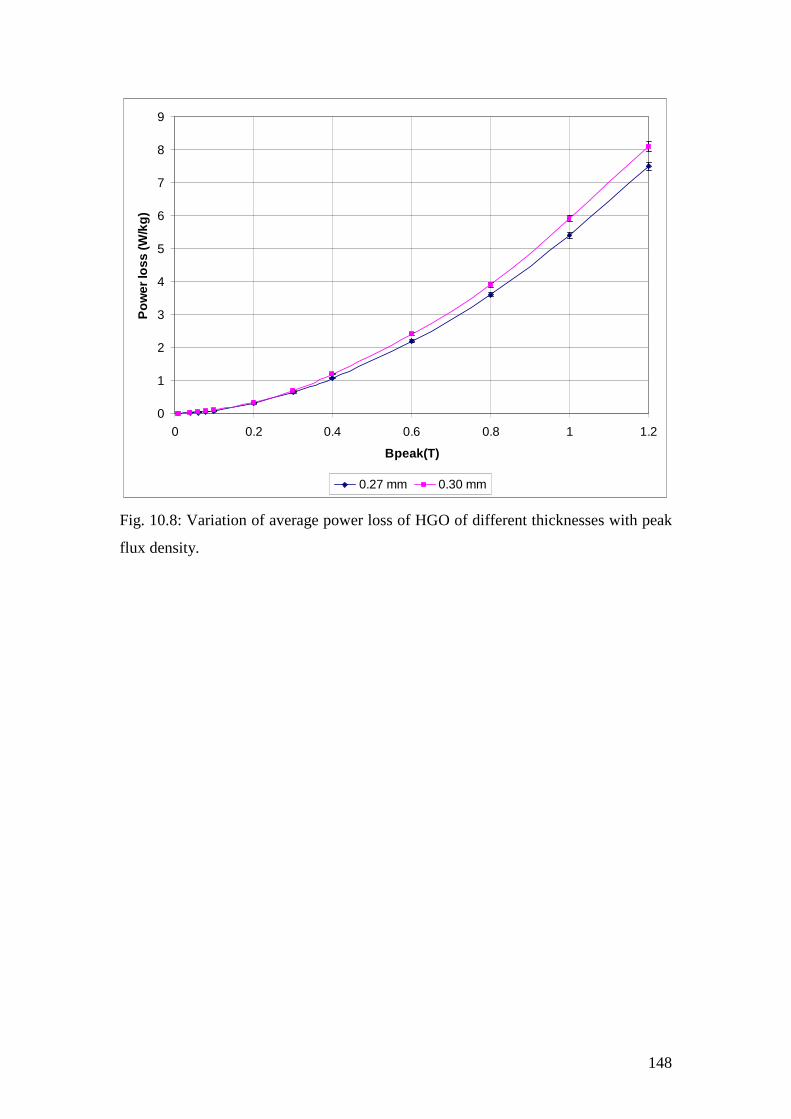
148

0

1

2

3

4

5

6

7

8

9

0 0.2 0.4 0.6 0.8 1 1.2

Bpeak(T)

Po

wer

loss

(W/k

g)

0.27 mm 0.30 mm

Fig. 10.8: Variation of average power loss of HGO of different thicknesses with peak

flux density.

149


[10.1] R. Ranjan, D. C. Jiles and P. K. Rastogi, Magnetic properties of decarburized


Transactions on Magnetics, Vol. 23 , No. 3, pp.1869-1876, 1987.

[10.2] D. G. Hwang, H.C Kim, C.G. Kim, K.A Lee, Barkhausen noise and magnetic

properties of highly grain-oriented HiB-8 and conventional 3% Si-Fe polycrystalline

specimens, Journal of Korean Physical Society, Vol. 24, No.6, pp. 493-498, 1991.

[10.3] F Brailsford, Physical principles of Magnetism, Van Nostrand, London, 1966.

150

Chapter 11 Conclusions and future work

11.1 Conclusions

BN in grain-oriented electrical steel at power frequency has different characteristics at

high and low flux density.

The larger BN signal of HGO compared to CGO at high flux densities occurs because

the grain size of HGO is on average higher than that of CGO. Increased grain size

enables domain walls to move further between pinning sites and so generate larger

changes in magnetization which results in larger BN signal. In addition, grain to grain

misorientation results in a strong suppression of the BN level. At low fields domain

walls exhibit a jerky motion consisting of random sequence of Barkhausen jumps

whose cumulative effect is higher in amplitude for CGO steels because of increase in

the number of grain boundaries and grain boundary area acting as pinning sites since

their fractional volume is larger.

Mechanically scribing HGO on one surface transverse to the rolling direction reduced

the BN amplitude at high flux densities. This is due to the decrease of domain width

by scribing. Then the trend reverses at low flux density. Scribing introduces local

strain which decreases domain wall spacing thereby limiting the mean free path of

domain walls.

Removal of the coating from the surface of grain-oriented electrical steel at power

frequency increase the BN due to the widening of the 180° domains as a result of the

release of the tensile stress imparted to the material during coating. The BN

characteristics of decoated samples with a 3 MPa tension applied were similar to

those observed before decoating demonstrating the close similarity between the

effects of coating stress and externally applied stress on BN due to their similar roles

in domain refinement. A strong correlation between average velocity of domain wall

movement and changes in BN in conventional and high permeability steels was found

which demonstrates that the dominant factor responsible for BN emission is the mean

free path of domain wall movement and hence the width of the predominant 180°

domains in these materials.

151

BN was also found to be directly proportional to externally applied tensile stress

especially at high flux density. As tensile stress is increased, more 180° domain walls

are created and this limits the width of domain walls thereby limiting the speed of

domain walls movement hence reducing Barkhausen noise amplitude. In this work

Barkhausen noise has proved to be a useful technique for detecting the stress

sensitivity of grain oriented electrical steel.

BN in grain-oriented electrical steel is affected by both average domain width and

thickness for strips 0.35 mm thick and above. It increases with increasing domain

width and decreases with increasing sample thickness owing to eddy current damping

effects. Domain width, hence grain size is the only influence on BN for strip

thicknesses below 0.35 mm, given the same microstructure.

BN on commercially produced non-oriented steel is influenced by silicon contents

and sample thickness. BN was found to increase with decreasing strip thickness and

increase with increasing silicon contents owing to eddy current shielding effects. The

rms values of the BN and the total sum of amplitudes were found to increase with the

rate of change of flux density at all the peak flux densities measured. The findings

show that the influence of sample thickness and silicon content is significant and must

be taken into consideration when measuring and interpreting BN in non-oriented

electrical steel.

152

11.2 Future work

This investigation has identified the need for further research especially in low field

magnetisation and dynamic domain observation in that regime.

There is limited magnetic data at low inductions and no account of the factors which

might control the B-H properties. Magnetic characteristics of GOES are measured at

high flux densities which are suitable for typical applications in power transformers.

The magnetic properties of materials are not usually specified over the low flux

density range used in metering current transformer cores and other low flux density

applications so performance at this level of magnetisation cannot be predicted with

measurements made at high inductions. Little headway is possible unless low flux

density characteristics are better assessed and understood.

Dynamic domain observation is required to ascertain the number of domain walls

that are active at low and high field magnetization regimes in CGO and HGO steels as

BN in electrical steel is principally caused by the movement of domain walls. It may

be discovered that dynamic domain observation especially at low fields will reveal

new magnetisation features which could be of importance in material development

and also to what extent non repeatable domain wall motion occur in that regime.

An extension of the magnetising frequency of the measurement system would be

useful as measurements were made at 50 Hz in this work. It will be interesting to

observe if similar relationships of BN and magnetic properties seen in this work still

exist at higher frequencies.

Further work could also be carried out to understand more the metallurgy of the

samples used in this work to have a greater understanding of the results observed in

this work.

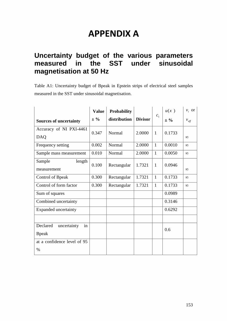
153

APPENDIX A

Uncertainty budget of the various parameters measured in the SST under sinusoidal magnetisation at 50 Hz

Table A1: Uncertainty budget of Bpeak in Epstein strips of electrical steel samples

measured in the SST under sinusoidal magnetisation.

Sources of uncertainty

Value

± %

Probability

distribution

Divisor 1c

)(xu

± %

iv or

effv

Accuracy of NI PXI-4461

DAQ 0.347 Normal 2.0000 1 0.1733

∞

Frequency setting 0.002 Normal 2.0000 1 0.0010 ∞

Sample mass measurement 0.010 Normal 2.0000 1 0.0050 ∞

Sample length

measurement 0.100 Rectangular 1.7321 1 0.0946

∞

Control of Bpeak 0.300 Rectangular 1.7321 1 0.1733 ∞

Control of form factor 0.300 Rectangular 1.7321 1 0.1733 ∞

Sum of squares 0.0989

Combined uncertainty 0.3146

Expanded uncertainty 0.6292

Declared uncertainty in

Bpeak 0.6

at a confidence level of 95

%

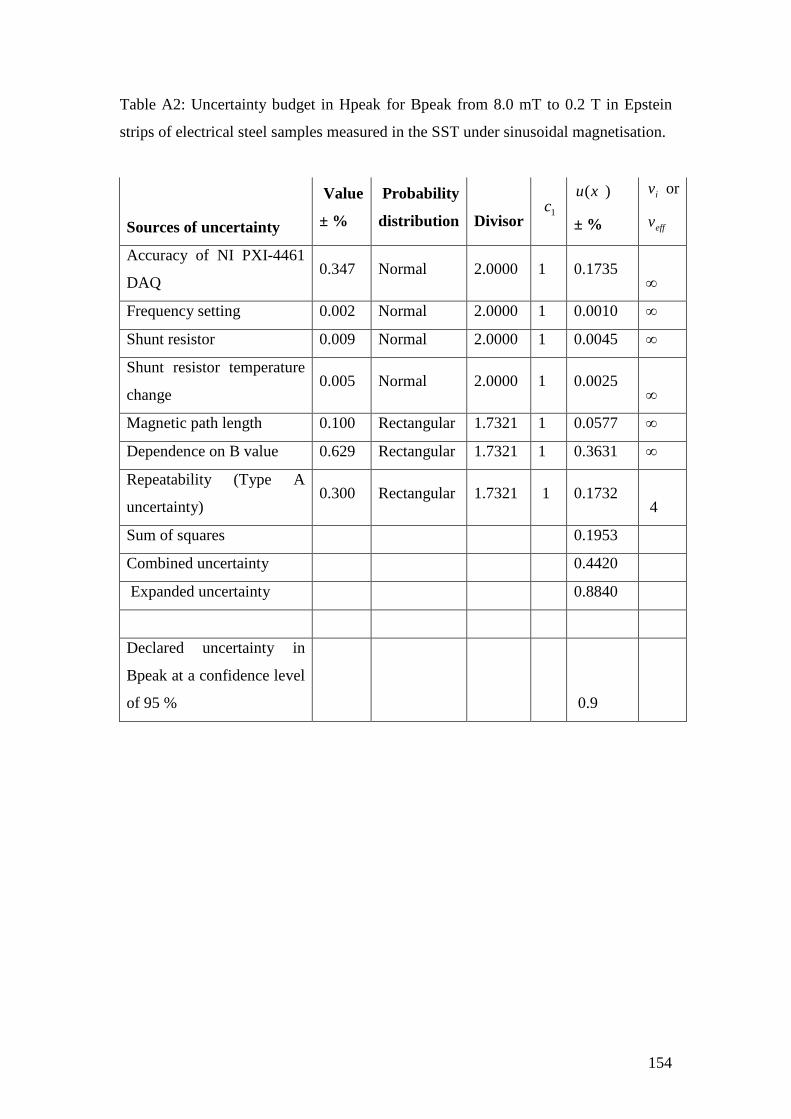
154

Table A2: Uncertainty budget in Hpeak for Bpeak from 8.0 mT to 0.2 T in Epstein



Value

± %

Probability

distribution

Divisor 1c

)(xu

± %

iv or

effv


DAQ 0.347 Normal 2.0000 1 0.1735

∞


Shunt resistor 0.009 Normal 2.0000 1 0.0045 ∞

Shunt resistor temperature

change 0.005 Normal 2.0000 1 0.0025

∞

Magnetic path length 0.100 Rectangular 1.7321 1 0.0577 ∞

Dependence on B value 0.629 Rectangular 1.7321 1 0.3631 ∞

Repeatability (Type A

uncertainty) 0.300 Rectangular 1.7321 1 0.1732

4





Bpeak at a confidence level

of 95 % 0.9

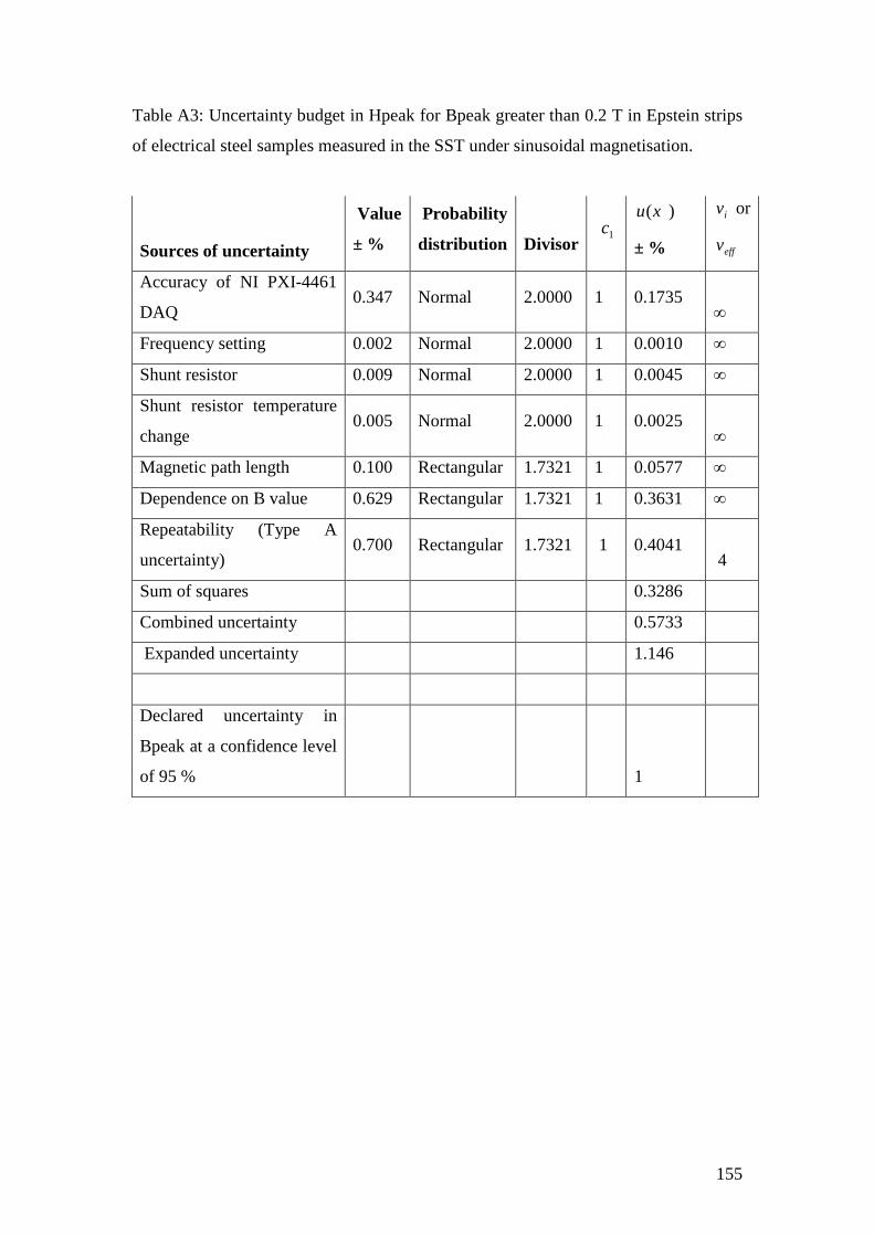
155

Table A3: Uncertainty budget in Hpeak for Bpeak greater than 0.2 T in Epstein strips

of electrical steel samples measured in the SST under sinusoidal magnetisation.


Value

± %

Probability

distribution

Divisor 1c

)(xu

± %

iv or

effv


DAQ 0.347 Normal 2.0000 1 0.1735

∞


Shunt resistor 0.009 Normal 2.0000 1 0.0045 ∞

Shunt resistor temperature

change 0.005 Normal 2.0000 1 0.0025

∞

Magnetic path length 0.100 Rectangular 1.7321 1 0.0577 ∞




4






of 95 % 1

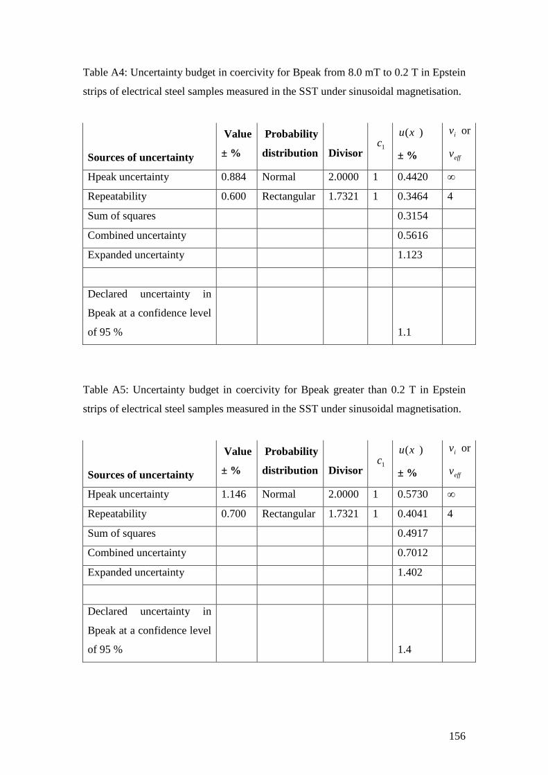
156

Table A4: Uncertainty budget in coercivity for Bpeak from 8.0 mT to 0.2 T in Epstein



Value

± %

Probability

distribution

Divisor 1c

)(xu

± %

iv or

effv

Hpeak uncertainty 0.884 Normal 2.0000 1 0.4420 ∞

Repeatability 0.600 Rectangular 1.7321 1 0.3464 4






of 95 % 1.1

Table A5: Uncertainty budget in coercivity for Bpeak greater than 0.2 T in Epstein



Value

± %

Probability

distribution

Divisor 1c

)(xu

± %

iv or

effv








of 95 % 1.4

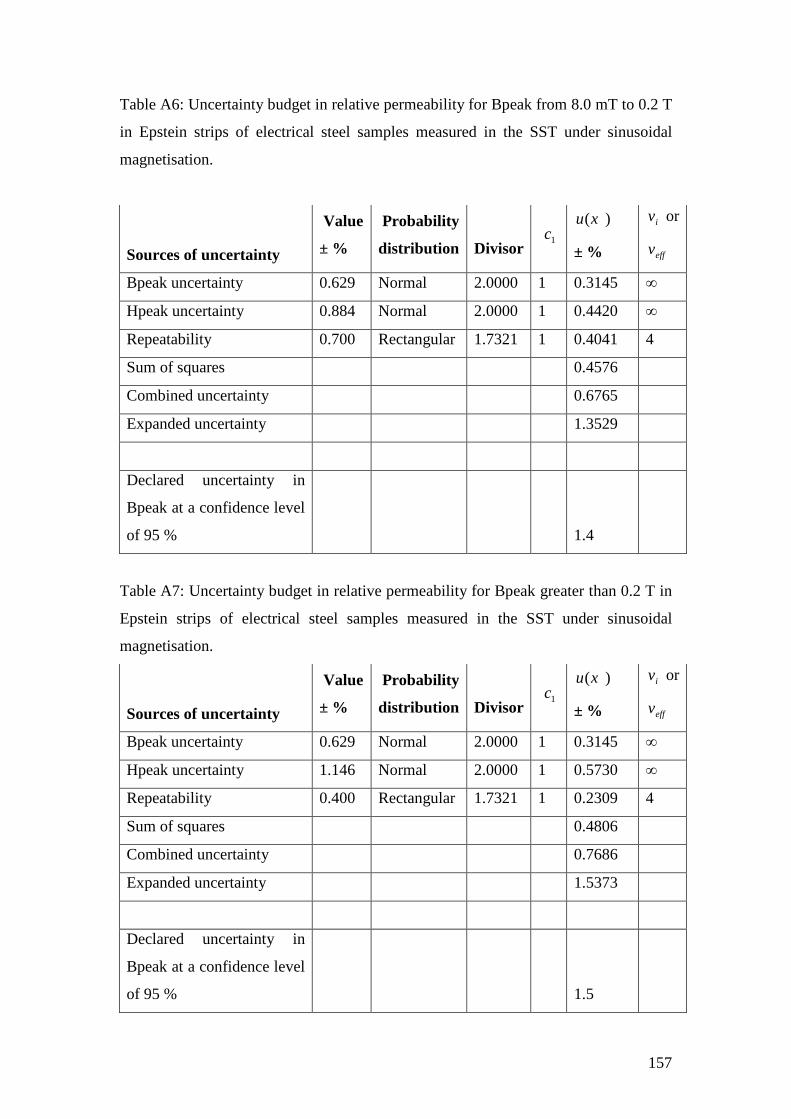
157

Table A6: Uncertainty budget in relative permeability for Bpeak from 8.0 mT to 0.2 T


magnetisation.


Value

± %

Probability

distribution

Divisor 1c

)(xu

± %

iv or

effv

Bpeak uncertainty 0.629 Normal 2.0000 1 0.3145 ∞








of 95 % 1.4

Table A7: Uncertainty budget in relative permeability for Bpeak greater than 0.2 T in


magnetisation.


Value

± %

Probability

distribution

Divisor 1c

)(xu

± %

iv or

effv









of 95 % 1.5

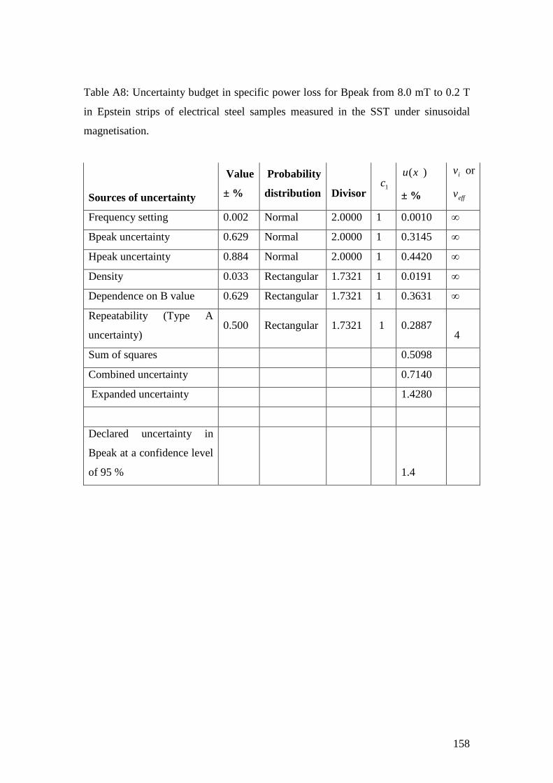
158

Table A8: Uncertainty budget in specific power loss for Bpeak from 8.0 mT to 0.2 T


magnetisation.


Value

± %

Probability

distribution

Divisor 1c

)(xu

± %

iv or

effv




Density 0.033 Rectangular 1.7321 1 0.0191 ∞




4






of 95 % 1.4

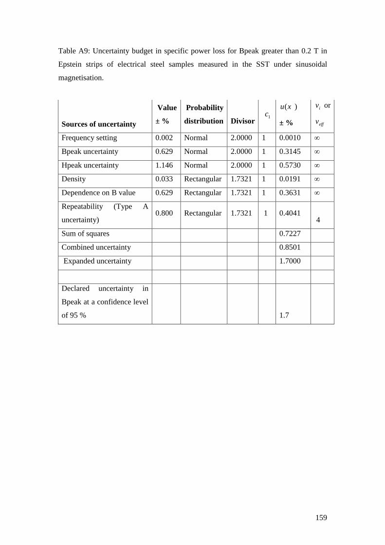
159

Table A9: Uncertainty budget in specific power loss for Bpeak greater than 0.2 T in


magnetisation.


Value

± %

Probability

distribution

Divisor 1c

)(xu

± %

iv or

effv




Density 0.033 Rectangular 1.7321 1 0.0191 ∞




4






of 95 % 1.7

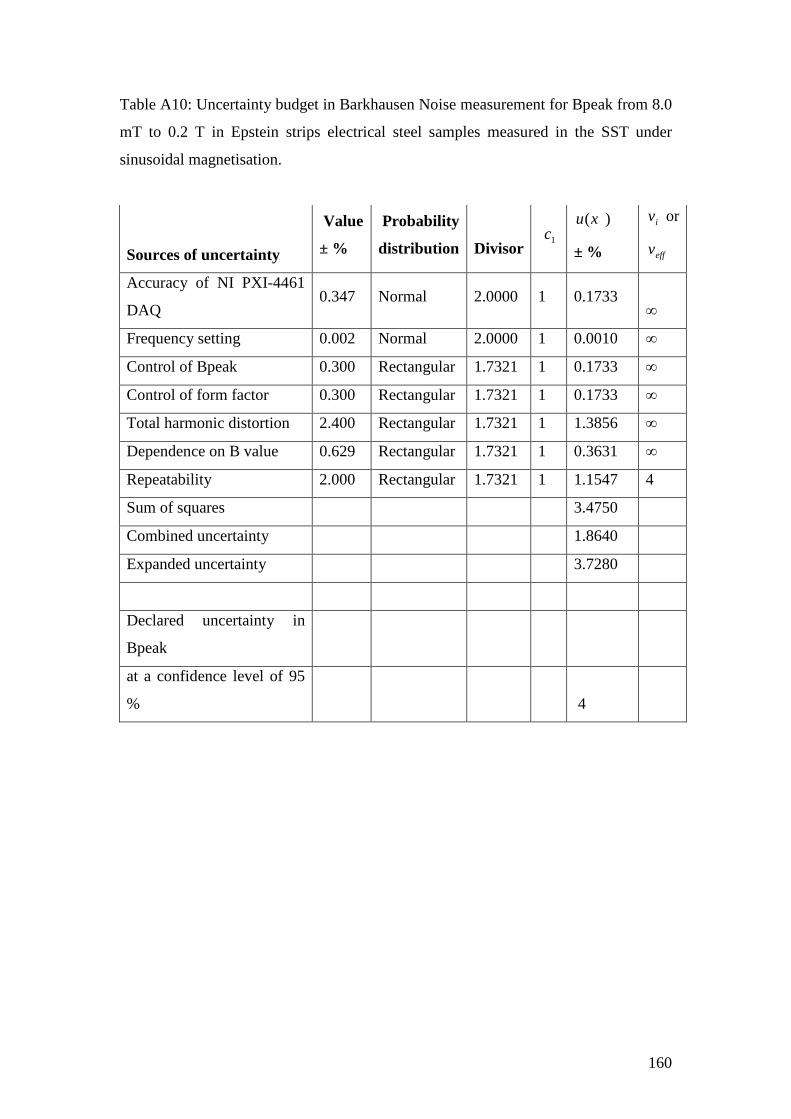
160

Table A10: Uncertainty budget in Barkhausen Noise measurement for Bpeak from 8.0

mT to 0.2 T in Epstein strips electrical steel samples measured in the SST under

sinusoidal magnetisation.


Value

± %

Probability

distribution

Divisor 1c

)(xu

± %

iv or

effv


DAQ 0.347 Normal 2.0000 1 0.1733

∞




Total harmonic distortion 2.400 Rectangular 1.7321 1 1.3856 ∞







Bpeak

at a confidence level of 95

% 4

161

Table A11: Uncertainty budget in Barkhausen Noise measurement for Bpeak greater

than 0.2 T in Epstein strips of electrical steel samples measured in the SST under

sinusoidal magnetisation.


Value

± %

Probability

distribution

Divisor 1c

)(xu

± %

iv or

effv


DAQ 0.347 Normal 2.0000 1 0.1733

∞




Total harmonic distortion 2.400 Rectangular 1.7321 1 1.3856 ∞








of 95 %

3.5

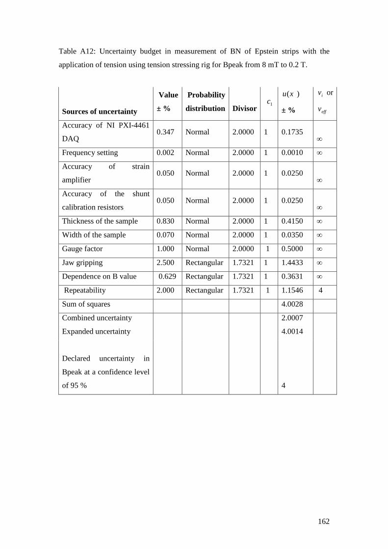
162

Table A12: Uncertainty budget in measurement of BN of Epstein strips with the

application of tension using tension stressing rig for Bpeak from 8 mT to 0.2 T.


Value

± %

Probability

distribution

Divisor 1c

)(xu

± %

iv or

effv


DAQ 0.347 Normal 2.0000 1 0.1735

∞


Accuracy of strain

amplifier 0.050 Normal 2.0000 1 0.0250

∞

Accuracy of the shunt

calibration resistors 0.050 Normal 2.0000 1 0.0250

∞

Thickness of the sample 0.830 Normal 2.0000 1 0.4150 ∞

Width of the sample 0.070 Normal 2.0000 1 0.0350 ∞

Gauge factor 1.000 Normal 2.0000 1 0.5000 ∞

Jaw gripping 2.500 Rectangular 1.7321 1 1.4433 ∞








of 95 % 4

163

Table A13: Uncertainty budget in measurement of BN of Epstein strips with the

application of tension using tension stressing rig for Bpeak above 0.2 T.


Value

± %

Probability

distribution

Divisor 1c

)(xu

± %

iv or

effv


DAQ 0.347 Normal 2.0000 1 0.1735

∞


Accuracy of strain

amplifier 0.050 Normal 2.0000 1 0.0250

∞

Accuracy of the shunt

calibration resistors 0.050 Normal 2.0000 1 0.0250

∞

Thickness of the sample 0.830 Normal 2.0000 1 0.4150 ∞

Width of the sample 0.070 Normal 2.0000 1 0.0350 ∞

Gauge factor 1.000 Normal 2.0000 1 0.5000 ∞

Jaw gripping 2.500 Rectangular 1.7321 1 1.4433 ∞








of 95 % 3.5

164

Appendix B

List of type A uncertainty of measurements

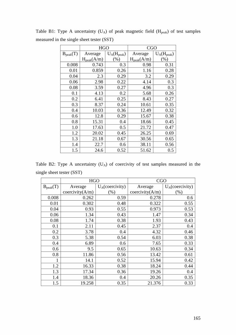
165

Table B1: Type A uncertainty (UA) of peak magnetic field (Hpeak) of test samples

measured in the single sheet tester (SST)

HGO CGO Bpeak(T) Average

Hpeak(A/m) UA(Hpeak)

(%) Average

Hpeak(A/m) UA(Hpeak)

(%) 0.008 0.743 0.3 0.98 0.31 0.01 0.859 0.26 1.16 0.28 0.04 2.3 0.29 3.2 0.29 0.06 2.98 0.22 4.14 0.3 0.08 3.59 0.27 4.96 0.3 0.1 4.13 0.2 5.68 0.26 0.2 6.41 0.25 8.43 0.27 0.3 8.37 0.24 10.61 0.35 0.4 10.03 0.36 12.49 0.32 0.6 12.8 0.29 15.67 0.38 0.8 15.31 0.4 18.66 0.45 1.0 17.63 0.5 21.72 0.47 1.2 20.02 0.45 26.25 0.69 1.3 21.18 0.67 30.56 0.65 1.4 22.7 0.6 38.11 0.56 1.5 24.6 0.52 51.62 0.5

Table B2: Type A uncertainty (UA) of coercivity of test samples measured in the

single sheet tester (SST)


coercivity(A/m) UA(coercivity)

(%) Average

coercivity(A/m) UA(coercivity)

(%) 0.008 0.262 0.59 0.278 0.6 0.01 0.302 0.48 0.322 0.55 0.04 0.93 0.55 0.973 0.53 0.06 1.34 0.43 1.47 0.34 0.08 1.74 0.38 1.93 0.43 0.1 2.11 0.45 2.37 0.4 0.2 3.78 0.4 4.32 0.46 0.3 5.38 0.54 6.03 0.38 0.4 6.89 0.6 7.65 0.33 0.6 9.5 0.65 10.63 0.34 0.8 11.86 0.56 13.42 0.61

1 14.1 0.52 15.94 0.42 1.2 16.33 0.38 18.24 0.44 1.3 17.34 0.36 19.26 0.4 1.4 18.36 0.4 20.26 0.35 1.5 19.258 0.35 21.376 0.33

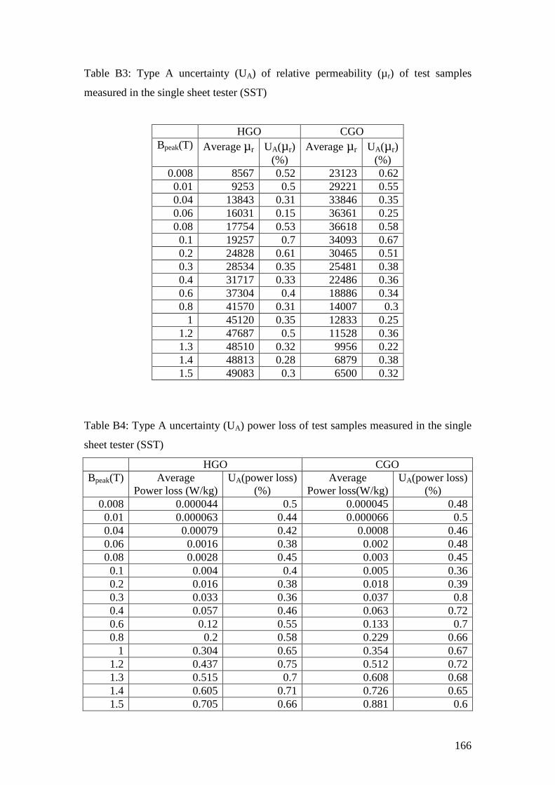
166

Table B3: Type A uncertainty (UA) of relative permeability (µr) of test samples

measured in the single sheet tester (SST)

HGO CGO Bpeak(T) Average µr UA(µr)

(%) Average µr

UA(µr)

(%) 0.008 8567 0.52 23123 0.62 0.01 9253 0.5 29221 0.55 0.04 13843 0.31 33846 0.35 0.06 16031 0.15 36361 0.25 0.08 17754 0.53 36618 0.58 0.1 19257 0.7 34093 0.67 0.2 24828 0.61 30465 0.51 0.3 28534 0.35 25481 0.38 0.4 31717 0.33 22486 0.36 0.6 37304 0.4 18886 0.34 0.8 41570 0.31 14007 0.3

1 45120 0.35 12833 0.25 1.2 47687 0.5 11528 0.36 1.3 48510 0.32 9956 0.22 1.4 48813 0.28 6879 0.38 1.5 49083 0.3 6500 0.32

Table B4: Type A uncertainty (UA) power loss of test samples measured in the single

sheet tester (SST)


Power loss (W/kg) UA(power loss)

(%) Average

Power loss(W/kg) UA(power loss)

(%) 0.008 0.000044 0.5 0.000045 0.48 0.01 0.000063 0.44 0.000066 0.5 0.04 0.00079 0.42 0.0008 0.46 0.06 0.0016 0.38 0.002 0.48 0.08 0.0028 0.45 0.003 0.45 0.1 0.004 0.4 0.005 0.36 0.2 0.016 0.38 0.018 0.39 0.3 0.033 0.36 0.037 0.8 0.4 0.057 0.46 0.063 0.72 0.6 0.12 0.55 0.133 0.7 0.8 0.2 0.58 0.229 0.66

1 0.304 0.65 0.354 0.67 1.2 0.437 0.75 0.512 0.72 1.3 0.515 0.7 0.608 0.68 1.4 0.605 0.71 0.726 0.65 1.5 0.705 0.66 0.881 0.6

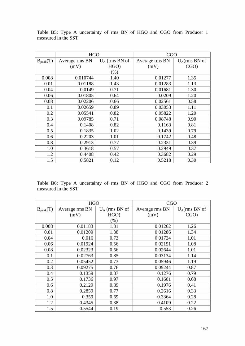
167

Table B5: Type A uncertainty of rms BN of HGO and CGO from Producer 1 measured in the SST

HGO CGO Bpeak(T) Average rms BN

(mV) UA (rms BN of

HGO) (%)

Average rms BN (mV)

UA(rms BN of CGO)

0.008 0.010744 1.40 0.01277 1.35 0.01 0.01188 1.43 0.01283 1.13 0.04 0.0149 0.71 0.01681 1.30 0.06 0.01805 0.64 0.0209 1.20 0.08 0.02206 0.66 0.02561 0.58 0.1 0.02659 0.89 0.03053 1.11 0.2 0.05541 0.82 0.05822 1.20 0.3 0.09785 0.71 0.08748 0.90 0.4 0.1408 0.82 0.1163 0.81 0.5 0.1835 1.02 0.1439 0.79 0.6 0.2203 1.01 0.1742 0.48 0.8 0.2913 0.77 0.2331 0.39 1.0 0.3618 0.57 0.2949 0.37 1.2 0.4408 0.42 0.3682 0.29 1.5 0.5821 0.12 0.5218 0.30

Table B6: Type A uncertainty of rms BN of HGO and CGO from Producer 2 measured in the SST

HGO CGO Bpeak(T) Average rms BN

(mV) UA (rms BN of

HGO) (%)

Average rms BN (mV)

UA(rms BN of CGO)

0.008 0.01183 1.31 0.01262 1.26 0.01 0.01209 1.38 0.01286 1.34 0.04 0.016 0.73 0.01724 1.01 0.06 0.01924 0.56 0.02151 1.08 0.08 0.02323 0.56 0.02644 1.01 0.1 0.02763 0.85 0.03134 1.14 0.2 0.05452 0.73 0.05946 1.19 0.3 0.09275 0.76 0.09244 0.87 0.4 0.1359 0.87 0.1276 0.79 0.5 0.1736 0.97 0.1601 0.68 0.6 0.2129 0.89 0.1976 0.41 0.8 0.2859 0.77 0.2616 0.33 1.0 0.359 0.69 0.3364 0.28 1.2 0.4345 0.38 0.4109 0.22 1.5 0.5544 0.19 0.553 0.26

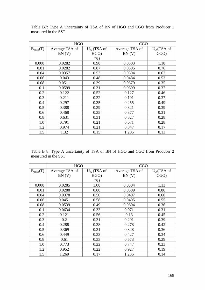
168

Table B7: Type A uncertainty of TSA of BN of HGO and CGO from Producer 1 measured in the SST

HGO CGO Bpeak(T) Average TSA of

BN (V) UA (TSA of

HGO) (%)

Average TSA of BN (V)

UA(TSA of CGO)

0.008 0.0282 0.98 0.0303 1.18 0.01 0.0282 0.87 0.0305 0.76 0.04 0.0357 0.53 0.0394 0.62 0.06 0.043 0.48 0.0484 0.53 0.08 0.0511 0.39 0.0579 0.35 0.1 0.0599 0.31 0.0699 0.37 0.2 0.122 0.52 0.127 0.46 0.3 0.211 0.32 0.191 0.37 0.4 0.297 0.35 0.255 0.49 0.5 0.388 0.29 0.321 0.39 0.6 0.468 0.35 0.377 0.31 0.8 0.631 0.31 0.527 0.28 1.0 0.791 0.21 0.671 0.28 1.2 0.974 0.21 0.847 0.17 1.5 1.32 0.15 1.205 0.13

Table B 8: Type A uncertainty of TSA of BN of HGO and CGO from Producer 2 measured in the SST

HGO CGO Bpeak(T) Average TSA of

BN (V) UA (TSA of

HGO) (%)

Average TSA of BN (V)

UA(TSA of CGO)

0.008 0.0285 1.08 0.0304 1.13 0.01 0.0288 0.88 0.0309 0.86 0.04 0.0378 0.50 0.0407 0.60 0.06 0.0451 0.58 0.0495 0.55 0.08 0.0539 0.49 0.0604 0.36 0.1 0.0634 0.33 0.071 0.31 0.2 0.121 0.56 0.13 0.45 0.3 0.2 0.31 0.201 0.39 0.4 0.288 0.38 0.278 0.42 0.5 0.369 0.31 0.348 0.36 0.6 0.449 0.33 0.427 0.34 0.8 0.61 0.33 0.573 0.29 1.0 0.773 0.22 0.747 0.23 1.2 0.952 0.22 0.927 0.19 1.5 1.269 0.17 1.235 0.14

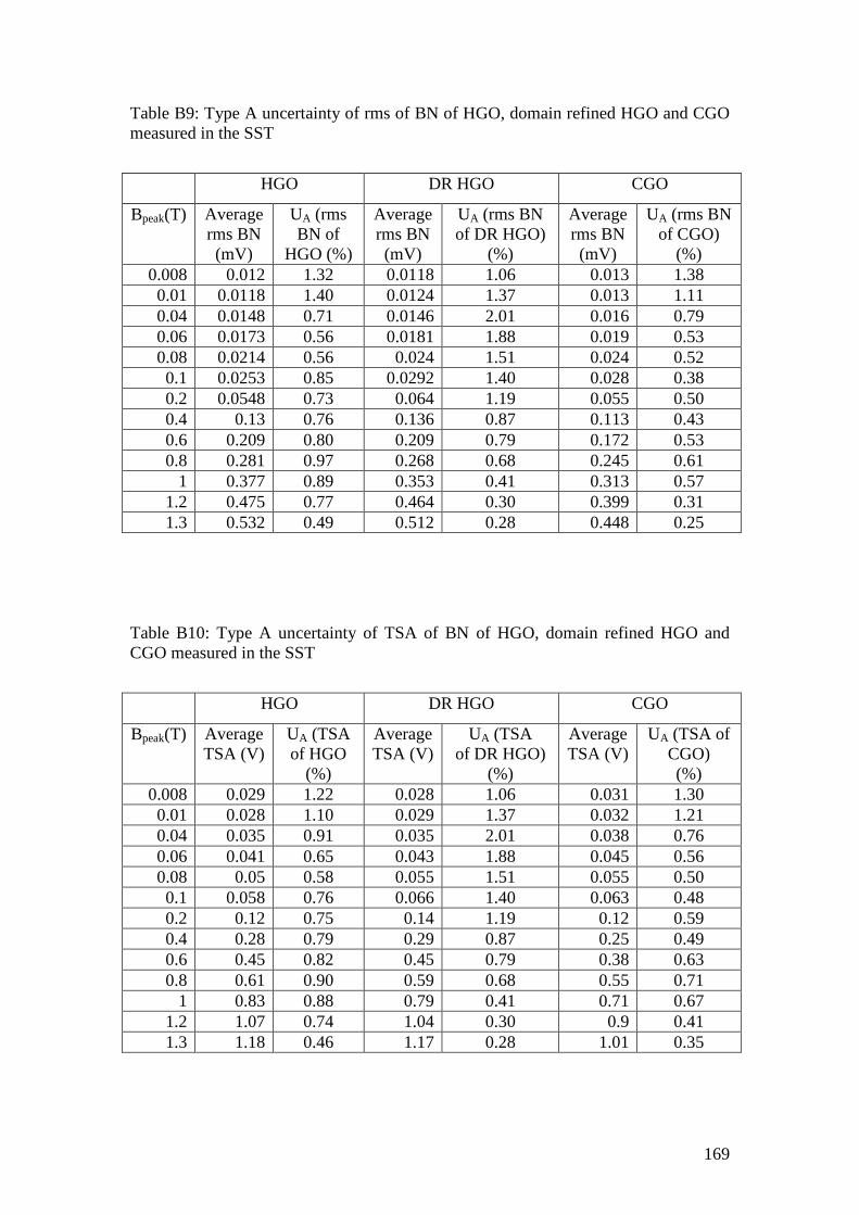
169

Table B9: Type A uncertainty of rms of BN of HGO, domain refined HGO and CGO measured in the SST

HGO DR HGO CGO

Bpeak(T) Average rms BN (mV)

UA (rms BN of

HGO (%)

Average rms BN (mV)

UA (rms BN of DR HGO)

(%)

Average rms BN (mV)

UA (rms BN of CGO)

(%) 0.008 0.012 1.32 0.0118 1.06 0.013 1.38 0.01 0.0118 1.40 0.0124 1.37 0.013 1.11 0.04 0.0148 0.71 0.0146 2.01 0.016 0.79 0.06 0.0173 0.56 0.0181 1.88 0.019 0.53 0.08 0.0214 0.56 0.024 1.51 0.024 0.52 0.1 0.0253 0.85 0.0292 1.40 0.028 0.38 0.2 0.0548 0.73 0.064 1.19 0.055 0.50 0.4 0.13 0.76 0.136 0.87 0.113 0.43 0.6 0.209 0.80 0.209 0.79 0.172 0.53 0.8 0.281 0.97 0.268 0.68 0.245 0.61

1 0.377 0.89 0.353 0.41 0.313 0.57 1.2 0.475 0.77 0.464 0.30 0.399 0.31 1.3 0.532 0.49 0.512 0.28 0.448 0.25

Table B10: Type A uncertainty of TSA of BN of HGO, domain refined HGO and CGO measured in the SST

HGO DR HGO CGO

Bpeak(T) Average TSA (V)

UA (TSA of HGO

(%)

Average TSA (V)

UA (TSA of DR HGO)

(%)

Average TSA (V)

UA (TSA of CGO) (%)

0.008 0.029 1.22 0.028 1.06 0.031 1.30 0.01 0.028 1.10 0.029 1.37 0.032 1.21 0.04 0.035 0.91 0.035 2.01 0.038 0.76 0.06 0.041 0.65 0.043 1.88 0.045 0.56 0.08 0.05 0.58 0.055 1.51 0.055 0.50 0.1 0.058 0.76 0.066 1.40 0.063 0.48 0.2 0.12 0.75 0.14 1.19 0.12 0.59 0.4 0.28 0.79 0.29 0.87 0.25 0.49 0.6 0.45 0.82 0.45 0.79 0.38 0.63 0.8 0.61 0.90 0.59 0.68 0.55 0.71

1 0.83 0.88 0.79 0.41 0.71 0.67 1.2 1.07 0.74 1.04 0.30 0.9 0.41 1.3 1.18 0.46 1.17 0.28 1.01 0.35

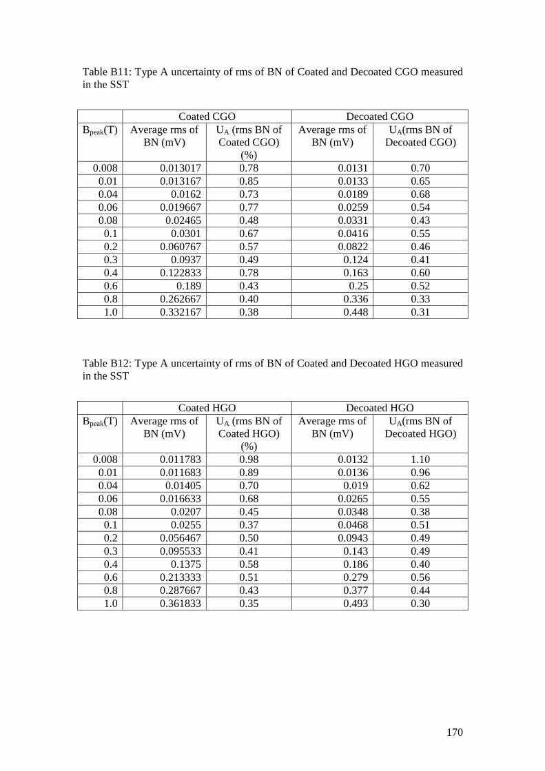
170

Table B11: Type A uncertainty of rms of BN of Coated and Decoated CGO measured in the SST

Coated CGO Decoated CGO Bpeak(T) Average rms of

BN (mV) UA (rms BN of Coated CGO)

(%)

Average rms of BN (mV)

UA(rms BN of Decoated CGO)

0.008 0.013017 0.78 0.0131 0.70 0.01 0.013167 0.85 0.0133 0.65 0.04 0.0162 0.73 0.0189 0.68 0.06 0.019667 0.77 0.0259 0.54 0.08 0.02465 0.48 0.0331 0.43 0.1 0.0301 0.67 0.0416 0.55 0.2 0.060767 0.57 0.0822 0.46 0.3 0.0937 0.49 0.124 0.41 0.4 0.122833 0.78 0.163 0.60 0.6 0.189 0.43 0.25 0.52 0.8 0.262667 0.40 0.336 0.33 1.0 0.332167 0.38 0.448 0.31

Table B12: Type A uncertainty of rms of BN of Coated and Decoated HGO measured in the SST

Coated HGO Decoated HGO Bpeak(T) Average rms of

BN (mV) UA (rms BN of Coated HGO)

(%)


UA(rms BN of Decoated HGO)

0.008 0.011783 0.98 0.0132 1.10 0.01 0.011683 0.89 0.0136 0.96 0.04 0.01405 0.70 0.019 0.62 0.06 0.016633 0.68 0.0265 0.55 0.08 0.0207 0.45 0.0348 0.38 0.1 0.0255 0.37 0.0468 0.51 0.2 0.056467 0.50 0.0943 0.49 0.3 0.095533 0.41 0.143 0.49 0.4 0.1375 0.58 0.186 0.40 0.6 0.213333 0.51 0.279 0.56 0.8 0.287667 0.43 0.377 0.44 1.0 0.361833 0.35 0.493 0.30

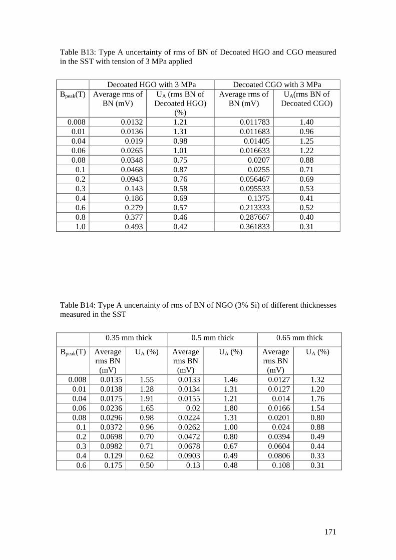
171

Table B13: Type A uncertainty of rms of BN of Decoated HGO and CGO measured in the SST with tension of 3 MPa applied

Decoated HGO with 3 MPa Decoated CGO with 3 MPa Bpeak(T) Average rms of

BN (mV) UA (rms BN of Decoated HGO)

(%)


UA(rms BN of Decoated CGO)

0.008 0.0132 1.21 0.011783 1.40 0.01 0.0136 1.31 0.011683 0.96 0.04 0.019 0.98 0.01405 1.25 0.06 0.0265 1.01 0.016633 1.22 0.08 0.0348 0.75 0.0207 0.88 0.1 0.0468 0.87 0.0255 0.71 0.2 0.0943 0.76 0.056467 0.69 0.3 0.143 0.58 0.095533 0.53 0.4 0.186 0.69 0.1375 0.41 0.6 0.279 0.57 0.213333 0.52 0.8 0.377 0.46 0.287667 0.40 1.0 0.493 0.42 0.361833 0.31

Table B14: Type A uncertainty of rms of BN of NGO (3% Si) of different thicknesses measured in the SST

0.35 mm thick 0.5 mm thick 0.65 mm thick


UA (%) Average rms BN (mV)


UA (%)

0.008 0.0135 1.55 0.0133 1.46 0.0127 1.32 0.01 0.0138 1.28 0.0134 1.31 0.0127 1.20 0.04 0.0175 1.91 0.0155 1.21 0.014 1.76 0.06 0.0236 1.65 0.02 1.80 0.0166 1.54 0.08 0.0296 0.98 0.0224 1.31 0.0201 0.80 0.1 0.0372 0.96 0.0262 1.00 0.024 0.88 0.2 0.0698 0.70 0.0472 0.80 0.0394 0.49 0.3 0.0982 0.71 0.0678 0.67 0.0604 0.44 0.4 0.129 0.62 0.0903 0.49 0.0806 0.33 0.6 0.175 0.50 0.13 0.48 0.108 0.31

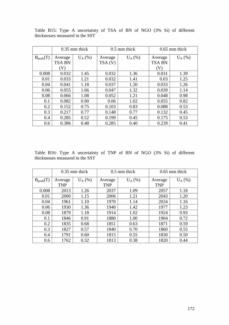
172

Table B15: Type A uncertainty of TSA of BN of NGO (3% Si) of different thicknesses measured in the SST


Bpeak(T) Average TSA BN

(V)

UA (%) Average TSA (V)

UA (%) Average TSA BN

(V)

UA (%)

0.008 0.032 1.45 0.032 1.36 0.031 1.39 0.01 0.033 1.21 0.032 1.41 0.03 1.25 0.04 0.041 1.18 0.037 1.20 0.033 1.26 0.06 0.055 1.66 0.047 1.32 0.039 1.14 0.08 0.066 1.08 0.052 1.21 0.048 0.98 0.1 0.082 0.90 0.06 1.02 0.055 0.82 0.2 0.152 0.75 0.103 0.83 0.088 0.53 0.3 0.217 0.77 0.148 0.77 0.132 0.45 0.4 0.285 0.52 0.199 0.45 0.175 0.53 0.6 0.386 0.48 0.285 0.40 0.239 0.41

Table B16: Type A uncertainty of TNP of BN of NGO (3% Si) of different thicknesses measured in the SST


Bpeak(T) Average TNP

UA (%) Average TNP

UA (%) Average TNP

UA (%)

0.008 2013 1.26 2037 1.09 2057 1.18 0.01 2000 1.15 2006 1.21 2043 1.20 0.04 1961 1.10 1970 1.14 2024 1.16 0.06 1930 1.36 1940 1.42 1977 1.23 0.08 1879 1.18 1914 1.02 1924 0.93 0.1 1846 0.91 1880 1.00 1904 0.72 0.2 1835 0.68 1851 0.63 1871 0.59 0.3 1827 0.57 1840 0.70 1860 0.55 0.4 1791 0.60 1815 0.55 1830 0.50 0.6 1762 0.32 1813 0.38 1820 0.44

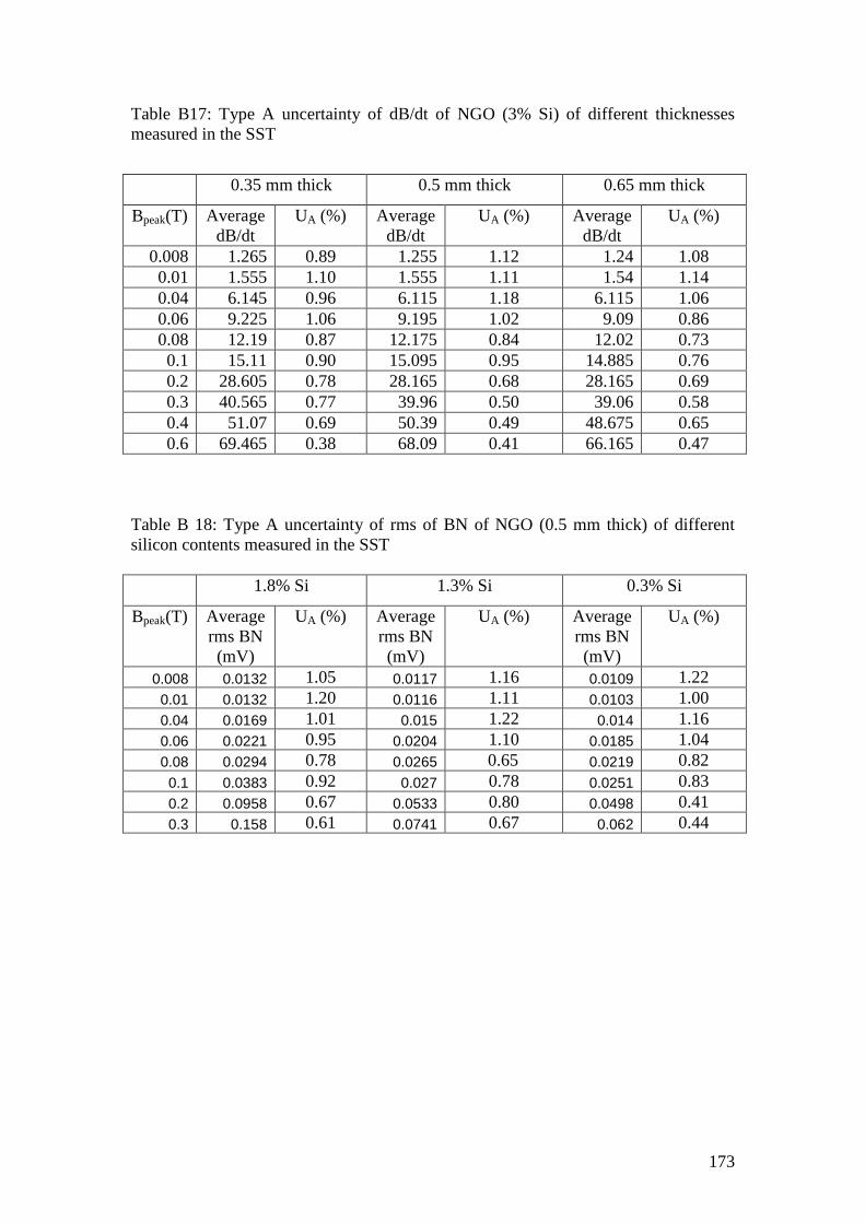
173

Table B17: Type A uncertainty of dB/dt of NGO (3% Si) of different thicknesses measured in the SST


Bpeak(T) Average dB/dt

UA (%) Average dB/dt


UA (%)

0.008 1.265 0.89 1.255 1.12 1.24 1.08 0.01 1.555 1.10 1.555 1.11 1.54 1.14 0.04 6.145 0.96 6.115 1.18 6.115 1.06 0.06 9.225 1.06 9.195 1.02 9.09 0.86 0.08 12.19 0.87 12.175 0.84 12.02 0.73 0.1 15.11 0.90 15.095 0.95 14.885 0.76 0.2 28.605 0.78 28.165 0.68 28.165 0.69 0.3 40.565 0.77 39.96 0.50 39.06 0.58 0.4 51.07 0.69 50.39 0.49 48.675 0.65 0.6 69.465 0.38 68.09 0.41 66.165 0.47

Table B 18: Type A uncertainty of rms of BN of NGO (0.5 mm thick) of different silicon contents measured in the SST 1.8% Si 1.3% Si 0.3% Si




UA (%)

0.008 0.0132 1.05 0.0117 1.16 0.0109 1.22 0.01 0.0132 1.20 0.0116 1.11 0.0103 1.00 0.04 0.0169 1.01 0.015 1.22 0.014 1.16 0.06 0.0221 0.95 0.0204 1.10 0.0185 1.04 0.08 0.0294 0.78 0.0265 0.65 0.0219 0.82 0.1 0.0383 0.92 0.027 0.78 0.0251 0.83 0.2 0.0958 0.67 0.0533 0.80 0.0498 0.41 0.3 0.158 0.61 0.0741 0.67 0.062 0.44

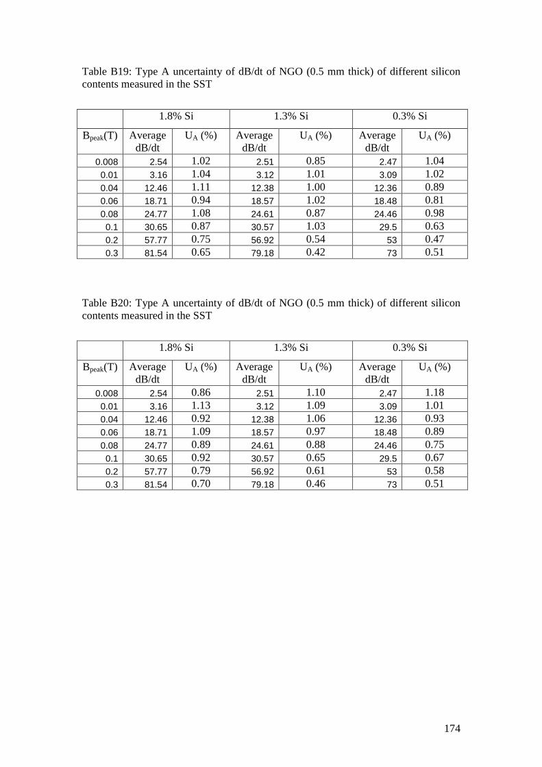
174

Table B19: Type A uncertainty of dB/dt of NGO (0.5 mm thick) of different silicon contents measured in the SST

1.8% Si 1.3% Si 0.3% Si




UA (%)

0.008 2.54 1.02 2.51 0.85 2.47 1.04 0.01 3.16 1.04 3.12 1.01 3.09 1.02 0.04 12.46 1.11 12.38 1.00 12.36 0.89 0.06 18.71 0.94 18.57 1.02 18.48 0.81 0.08 24.77 1.08 24.61 0.87 24.46 0.98 0.1 30.65 0.87 30.57 1.03 29.5 0.63 0.2 57.77 0.75 56.92 0.54 53 0.47 0.3 81.54 0.65 79.18 0.42 73 0.51

Table B20: Type A uncertainty of dB/dt of NGO (0.5 mm thick) of different silicon contents measured in the SST

1.8% Si 1.3% Si 0.3% Si




UA (%)

0.008 2.54 0.86 2.51 1.10 2.47 1.18 0.01 3.16 1.13 3.12 1.09 3.09 1.01 0.04 12.46 0.92 12.38 1.06 12.36 0.93 0.06 18.71 1.09 18.57 0.97 18.48 0.89 0.08 24.77 0.89 24.61 0.88 24.46 0.75 0.1 30.65 0.92 30.57 0.65 29.5 0.67 0.2 57.77 0.79 56.92 0.61 53 0.58 0.3 81.54 0.70 79.18 0.46 73 0.51

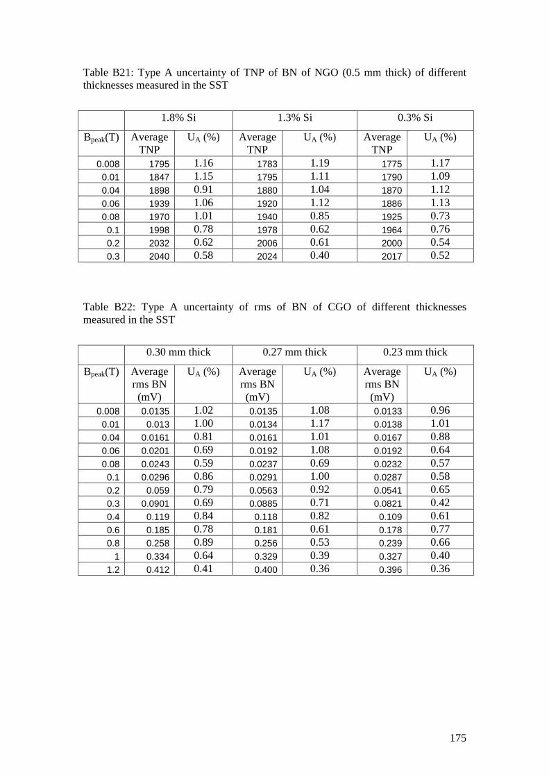
175

Table B21: Type A uncertainty of TNP of BN of NGO (0.5 mm thick) of different thicknesses measured in the SST

1.8% Si 1.3% Si 0.3% Si

Bpeak(T) Average TNP

UA (%) Average TNP

UA (%) Average TNP

UA (%)

0.008 1795 1.16 1783 1.19 1775 1.17 0.01 1847 1.15 1795 1.11 1790 1.09 0.04 1898 0.91 1880 1.04 1870 1.12 0.06 1939 1.06 1920 1.12 1886 1.13 0.08 1970 1.01 1940 0.85 1925 0.73 0.1 1998 0.78 1978 0.62 1964 0.76 0.2 2032 0.62 2006 0.61 2000 0.54 0.3 2040 0.58 2024 0.40 2017 0.52

Table B22: Type A uncertainty of rms of BN of CGO of different thicknesses measured in the SST





UA (%)

0.008 0.0135 1.02 0.0135 1.08 0.0133 0.96 0.01 0.013 1.00 0.0134 1.17 0.0138 1.01 0.04 0.0161 0.81 0.0161 1.01 0.0167 0.88 0.06 0.0201 0.69 0.0192 1.08 0.0192 0.64 0.08 0.0243 0.59 0.0237 0.69 0.0232 0.57 0.1 0.0296 0.86 0.0291 1.00 0.0287 0.58 0.2 0.059 0.79 0.0563 0.92 0.0541 0.65 0.3 0.0901 0.69 0.0885 0.71 0.0821 0.42 0.4 0.119 0.84 0.118 0.82 0.109 0.61 0.6 0.185 0.78 0.181 0.61 0.178 0.77 0.8 0.258 0.89 0.256 0.53 0.239 0.66

1 0.334 0.64 0.329 0.39 0.327 0.40 1.2 0.412 0.41 0.400 0.36 0.396 0.36

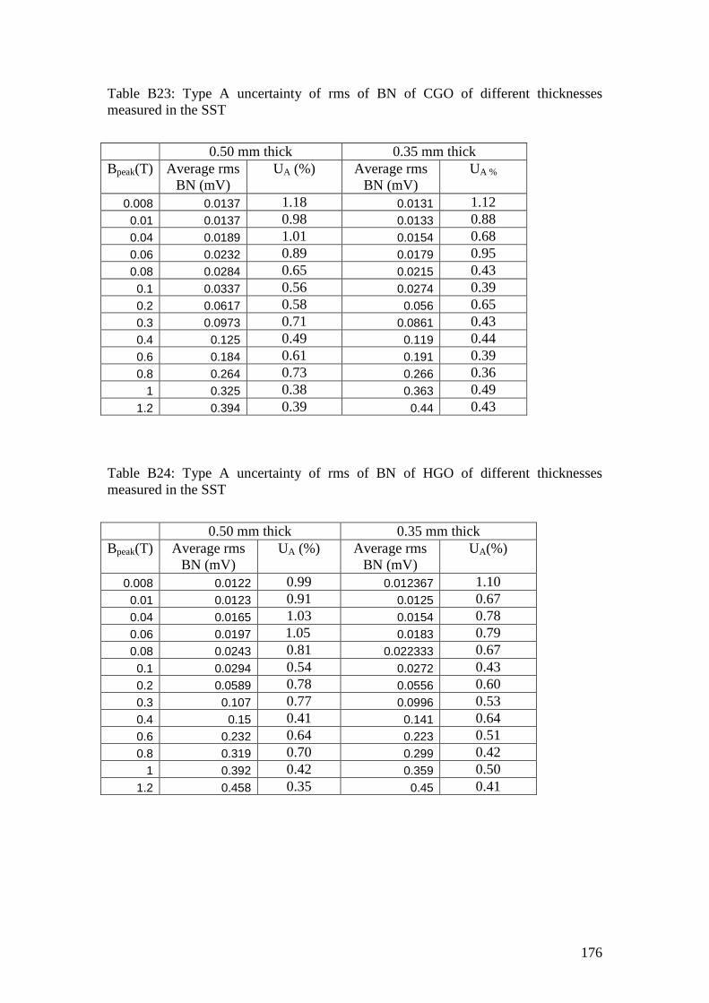
176

Table B23: Type A uncertainty of rms of BN of CGO of different thicknesses measured in the SST

0.50 mm thick 0.35 mm thick Bpeak(T) Average rms

BN (mV) UA (%) Average rms

BN (mV) UA %

0.008 0.0137 1.18 0.0131 1.12 0.01 0.0137 0.98 0.0133 0.88 0.04 0.0189 1.01 0.0154 0.68 0.06 0.0232 0.89 0.0179 0.95 0.08 0.0284 0.65 0.0215 0.43 0.1 0.0337 0.56 0.0274 0.39 0.2 0.0617 0.58 0.056 0.65 0.3 0.0973 0.71 0.0861 0.43 0.4 0.125 0.49 0.119 0.44 0.6 0.184 0.61 0.191 0.39 0.8 0.264 0.73 0.266 0.36

1 0.325 0.38 0.363 0.49 1.2 0.394 0.39 0.44 0.43

Table B24: Type A uncertainty of rms of BN of HGO of different thicknesses measured in the SST

0.50 mm thick 0.35 mm thick Bpeak(T) Average rms


BN (mV) UA(%)

0.008 0.0122 0.99 0.012367 1.10 0.01 0.0123 0.91 0.0125 0.67 0.04 0.0165 1.03 0.0154 0.78 0.06 0.0197 1.05 0.0183 0.79 0.08 0.0243 0.81 0.022333 0.67 0.1 0.0294 0.54 0.0272 0.43 0.2 0.0589 0.78 0.0556 0.60 0.3 0.107 0.77 0.0996 0.53 0.4 0.15 0.41 0.141 0.64 0.6 0.232 0.64 0.223 0.51 0.8 0.319 0.70 0.299 0.42

1 0.392 0.42 0.359 0.50 1.2 0.458 0.35 0.45 0.41

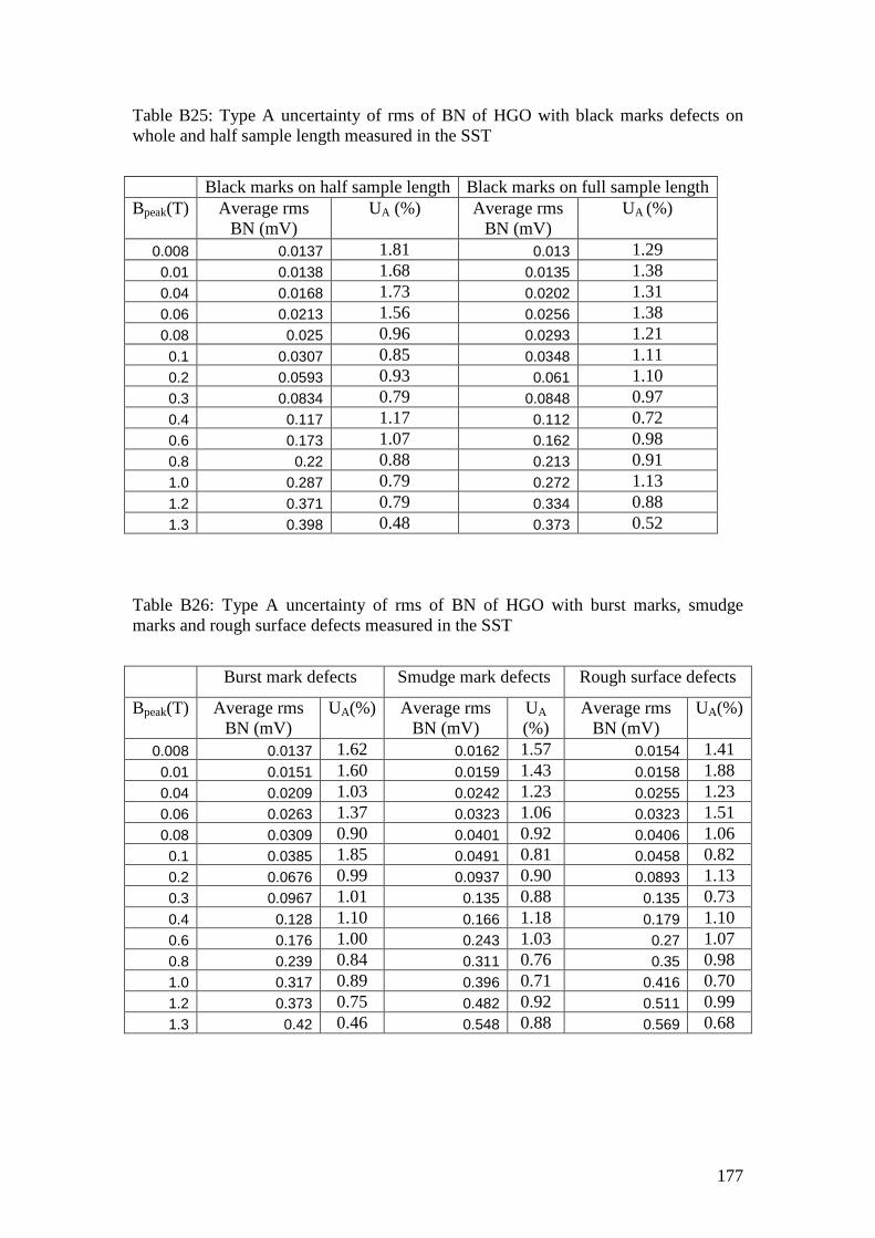
177

Table B25: Type A uncertainty of rms of BN of HGO with black marks defects on whole and half sample length measured in the SST

Black marks on half sample length Black marks on full sample length Bpeak(T) Average rms


BN (mV) UA (%)

0.008 0.0137 1.81 0.013 1.29 0.01 0.0138 1.68 0.0135 1.38 0.04 0.0168 1.73 0.0202 1.31 0.06 0.0213 1.56 0.0256 1.38 0.08 0.025 0.96 0.0293 1.21 0.1 0.0307 0.85 0.0348 1.11 0.2 0.0593 0.93 0.061 1.10 0.3 0.0834 0.79 0.0848 0.97 0.4 0.117 1.17 0.112 0.72 0.6 0.173 1.07 0.162 0.98 0.8 0.22 0.88 0.213 0.91 1.0 0.287 0.79 0.272 1.13 1.2 0.371 0.79 0.334 0.88 1.3 0.398 0.48 0.373 0.52

Table B26: Type A uncertainty of rms of BN of HGO with burst marks, smudge marks and rough surface defects measured in the SST

Burst mark defects Smudge mark defects Rough surface defects


UA(%) Average rms BN (mV)

UA (%)

Average rms BN (mV)

UA(%)

0.008 0.0137 1.62 0.0162 1.57 0.0154 1.41 0.01 0.0151 1.60 0.0159 1.43 0.0158 1.88 0.04 0.0209 1.03 0.0242 1.23 0.0255 1.23 0.06 0.0263 1.37 0.0323 1.06 0.0323 1.51 0.08 0.0309 0.90 0.0401 0.92 0.0406 1.06 0.1 0.0385 1.85 0.0491 0.81 0.0458 0.82 0.2 0.0676 0.99 0.0937 0.90 0.0893 1.13 0.3 0.0967 1.01 0.135 0.88 0.135 0.73 0.4 0.128 1.10 0.166 1.18 0.179 1.10 0.6 0.176 1.00 0.243 1.03 0.27 1.07 0.8 0.239 0.84 0.311 0.76 0.35 0.98 1.0 0.317 0.89 0.396 0.71 0.416 0.70 1.2 0.373 0.75 0.482 0.92 0.511 0.99 1.3 0.42 0.46 0.548 0.88 0.569 0.68

178

APPENDIX C Graphs of variations of percentage difference of the

measured properties at different peak flux densities

179

-15

-10

-5

0

5

10

0 0.2 0.4 0.6 0.8 1 1.2 1.4

Bpeak(T)

% D

iffer

ence

in B

Nrm

s

Fig. AC 1: Variation of percentage difference of average rms BN of HGO and domain

scribed HGO from P1 with peak flux density.

Fig. AC 2: Variation of percentage difference of average TSA of HGO and domain

scribed HGO from P1 with peak flux density.

-15

-10

-5

0

5

10

0 0.2 0.4 0.6 0.8 1 1.2 1.4

Bpeak(T)

% D

iffer

ence

in T

SA

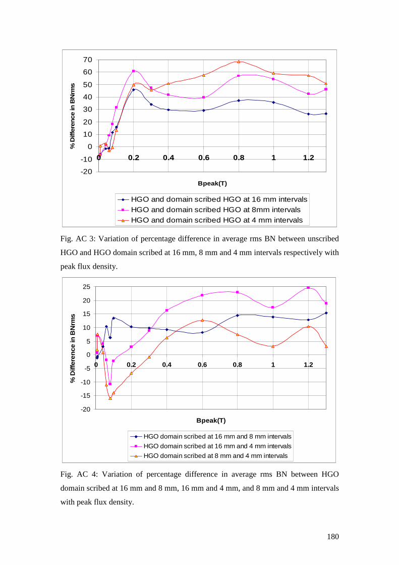
180

-20

-10

0

10

20

30

40

50

60

70

0 0.2 0.4 0.6 0.8 1 1.2

Bpeak(T)

% D

iffer

ence

in B

Nrm

s

HGO and domain scribed HGO at 16 mm intervalsHGO and domain scribed HGO at 8mm intervalsHGO and domain scribed HGO at 4 mm intervals

Fig. AC 3: Variation of percentage difference in average rms BN between unscribed


peak flux density.

-20

-15

-10

-5

0

5

10

15

20

25

0 0.2 0.4 0.6 0.8 1 1.2

Bpeak(T)

% D

iffer

ence

in B

Nrm

s

HGO domain scribed at 16 mm and 8 mm intervals



Fig. AC 4: Variation of percentage difference in average rms BN between HGO



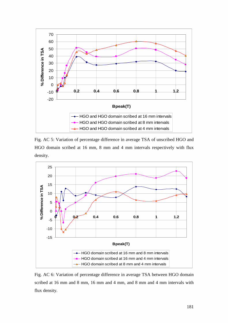
181

-20

-10

0

10

20

30

40

50

60

70

0 0.2 0.4 0.6 0.8 1 1.2

Bpeak(T)

% D

iffer

ence

in T

SA

HGO and HGO domain scribed at 16 mm intervals



Fig. AC 5: Variation of percentage difference in average TSA of unscribed HGO and

HGO domain scribed at 16 mm, 8 mm and 4 mm intervals respectively with flux

density.

-15

-10

-5

0

5

10

15

20

25

0 0.2 0.4 0.6 0.8 1 1.2

Bpeak(T)

% D

iffer

ence

in T

SA




Fig. AC 6: Variation of percentage difference in average TSA between HGO domain

scribed at 16 mm and 8 mm, 16 mm and 4 mm, and 8 mm and 4 mm intervals with

flux density.

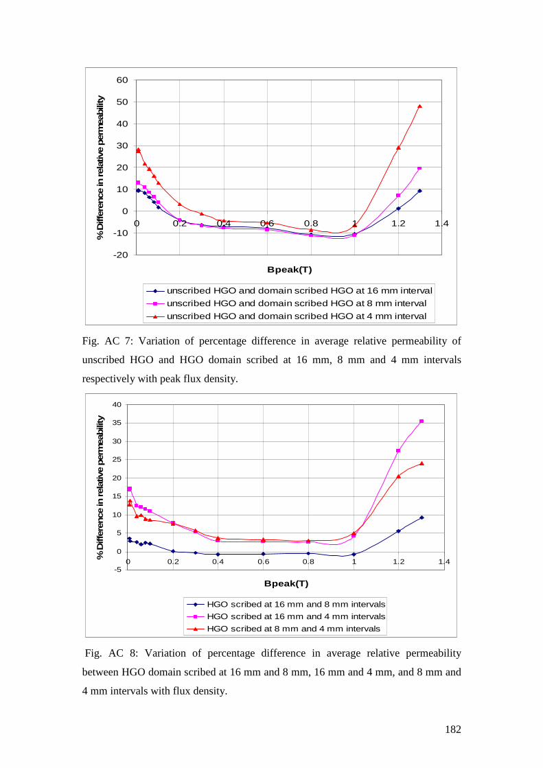
182

-20

-10

0

10

20

30

40

50

60

0 0.2 0.4 0.6 0.8 1 1.2 1.4

Bpeak(T)

% D

iffer

ence

in rel

ativ

e per

mea

bili

ty

unscribed HGO and domain scribed HGO at 16 mm interval



Fig. AC 7: Variation of percentage difference in average relative permeability of

unscribed HGO and HGO domain scribed at 16 mm, 8 mm and 4 mm intervals

respectively with peak flux density.

-5

0

5

10

15

20

25

30

35

40

0 0.2 0.4 0.6 0.8 1 1.2 1.4

Bpeak(T)

% D

iffer

ence

in rel

ativ

e per

mea

bili

ty

HGO scribed at 16 mm and 8 mm intervals



Fig. AC 8: Variation of percentage difference in average relative permeability

between HGO domain scribed at 16 mm and 8 mm, 16 mm and 4 mm, and 8 mm and

4 mm intervals with flux density.

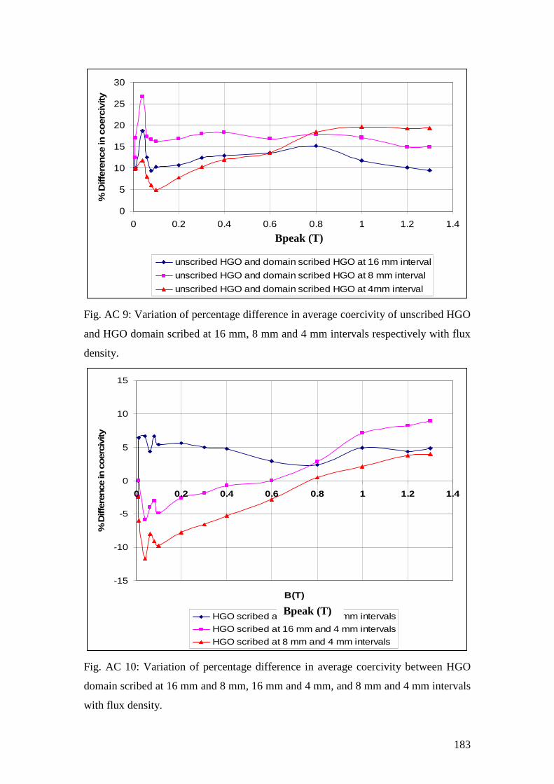
183

0

5

10

15

20

25

30

0 0.2 0.4 0.6 0.8 1 1.2 1.4

B(T)

% D

iffer

ence

in c

oer

civi

ty



unscribed HGO and domain scribed HGO at 4mm interval

Fig. AC 9: Variation of percentage difference in average coercivity of unscribed HGO

and HGO domain scribed at 16 mm, 8 mm and 4 mm intervals respectively with flux

density.

-15

-10

-5

0

5

10

15

0 0.2 0.4 0.6 0.8 1 1.2 1.4

B(T)

% D

iffer

ence

in c

oer

civi

ty




Fig. AC 10: Variation of percentage difference in average coercivity between HGO


with flux density.

Bpeak (T)

Bpeak (T)

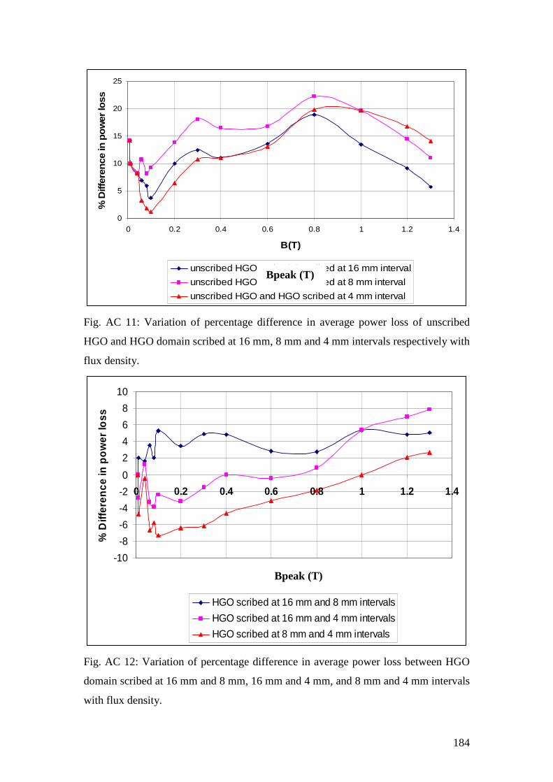
184

0

5

10

15

20

25

0 0.2 0.4 0.6 0.8 1 1.2 1.4

B(T)

% D

iffer

ence

in p

ow

er lo

ss

unscribed HGO and HGO scribed at 16 mm interval



Fig. AC 11: Variation of percentage difference in average power loss of unscribed


flux density.

-10

-8

-6

-4

-2

0

2

4

6

8

10

0 0.2 0.4 0.6 0.8 1 1.2 1.4

B(T)

% D

iffer

ence

in p

ow

er lo

ss




Fig. AC 12: Variation of percentage difference in average power loss between HGO


with flux density.

Bpeak (T)

Bpeak (T)

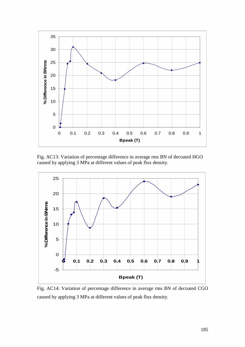
185

0

5

10

15

20

25

30

35

0 0.1 0.2 0.3 0.4 0.5 0.6 0.7 0.8 0.9 1

Bpeak (T)

% D

iffer

ence

in B

Nrm

s

Fig. AC13: Variation of percentage difference in average rms BN of decoated HGO caused by applying 3 MPa at different values of peak flux density.

-5

0

5

10

15

20

25

0 0.1 0.2 0.3 0.4 0.5 0.6 0.7 0.8 0.9 1

Bpeak (T)

% D

iffer

ence

in B

Nrm

s

Fig. AC14: Variation of percentage difference in average rms BN of decoated CGO

caused by applying 3 MPa at different values of peak flux density.

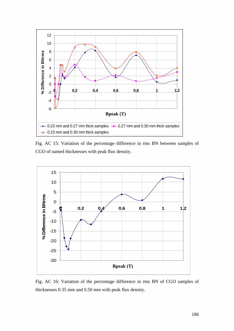
186

-6

-4

-2

0

2

4

6

8

10

12

0 0.2 0.4 0.6 0.8 1 1.2

B(T)

% D

iffer

ence

in B

Nrm

s

0.23 mm and 0.27 mm thick samples 0.27 mm and 0.30 mm thick samples

0.23 mm and 0.30 mm thick samples

Fig. AC 15: Variation of the percentage difference in rms BN between samples of

CGO of named thicknesses with peak flux density.

-30

-25

-20

-15

-10

-5

0

5

10

15

0 0.2 0.4 0.6 0.8 1 1.2

B(T)

% D

iffer

ence

in B

Nrm

s

Fig. AC 16: Variation of the percentage difference in rms BN of CGO samples of

thicknesses 0.35 mm and 0.50 mm with peak flux density.

Bpeak (T)

Bpeak (T)

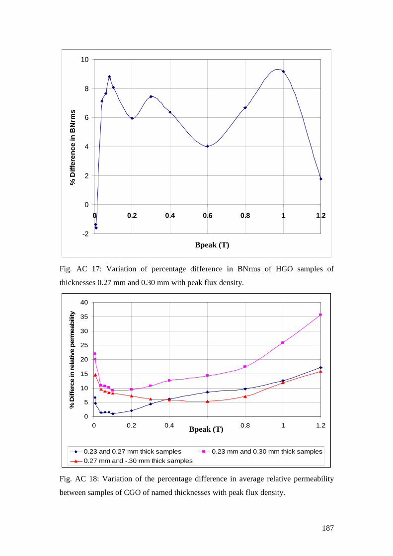
187

-2

0

2

4

6

8

10

0 0.2 0.4 0.6 0.8 1 1.2

B(T)

% D

iffer

ence

in B

Nrm

s

Fig. AC 17: Variation of percentage difference in BNrms of HGO samples of

thicknesses 0.27 mm and 0.30 mm with peak flux density.

0

5

10

15

20

25

30

35

40

0 0.2 0.4 0.6 0.8 1 1.2

B(T)

% D

iffer

ce in

rel

ativ

e p

erm

eab

ility

0.23 and 0.27 mm thick samples 0.23 mm and 0.30 mm thick samples

0.27 mm and -.30 mm thick samples

Fig. AC 18: Variation of the percentage difference in average relative permeability

between samples of CGO of named thicknesses with peak flux density.

Bpeak (T)

Bpeak (T)

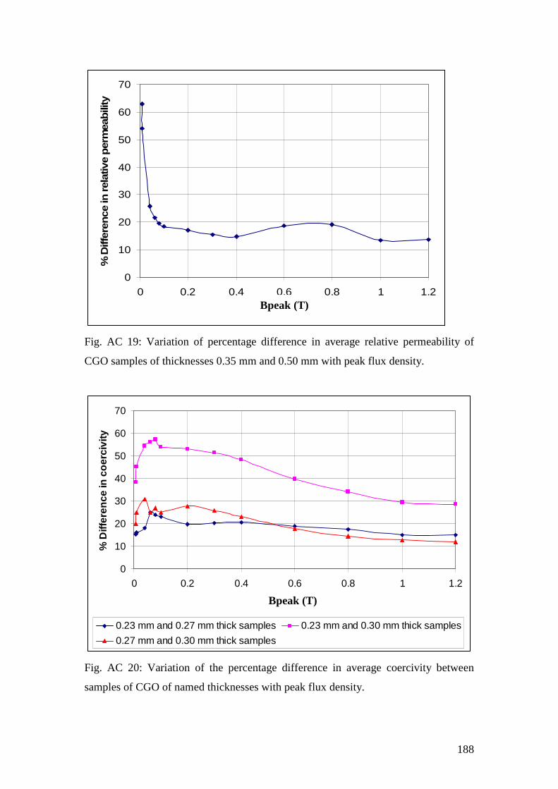
188

0

10

20

30

40

50

60

70

0 0.2 0.4 0.6 0.8 1 1.2

B(T)

% D

iffer

ence

in r

elat

ive

per

mea

bili

ty


CGO samples of thicknesses 0.35 mm and 0.50 mm with peak flux density.

0

10

20

30

40

50

60

70

0 0.2 0.4 0.6 0.8 1 1.2

B(T)

% D

iffer

ence

in c

oer

civi

ty

0.23 mm and 0.27 mm thick samples 0.23 mm and 0.30 mm thick samples


Fig. AC 20: Variation of the percentage difference in average coercivity between

samples of CGO of named thicknesses with peak flux density.

Bpeak (T)

Bpeak (T)

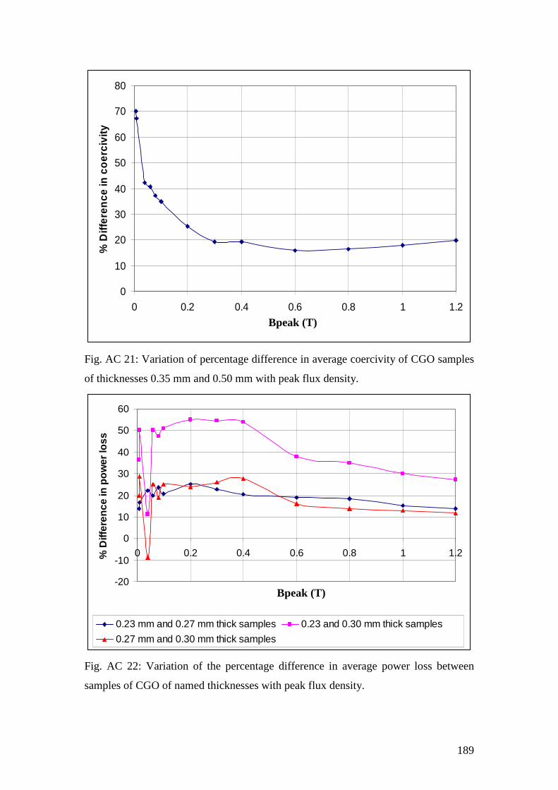
189

0

10

20

30

40

50

60

70

80

0 0.2 0.4 0.6 0.8 1 1.2

B(T)

% D

iffer

ence

in c

oer

civi

ty

Fig. AC 21: Variation of percentage difference in average coercivity of CGO samples

of thicknesses 0.35 mm and 0.50 mm with peak flux density.

-20

-10

0

10

20

30

40

50

60

0 0.2 0.4 0.6 0.8 1 1.2

B(T)

% D

iffer

ence

in p

ow

er lo

ss

0.23 mm and 0.27 mm thick samples 0.23 and 0.30 mm thick samples


Fig. AC 22: Variation of the percentage difference in average power loss between

samples of CGO of named thicknesses with peak flux density.

Bpeak (T)

Bpeak (T)

190

0

10

20

30

40

50

60

70

80

0 0.2 0.4 0.6 0.8 1 1.2

B(T)

% D

iffer

ence

in p

ow

er lo

ss

Fig. AC 23: Variation of percentage difference in average power loss of CGO samples


0

5

10

15

20

25

0 0.2 0.4 0.6 0.8 1 1.2

B(T)

% D

iffer

ence

in r

elat

ive

per

mea

bili

ty


HGO samples of thicknesses 0.27 mm and 0.30 mm with peak flux density.

Bpeak (T)

Bpeak (T)

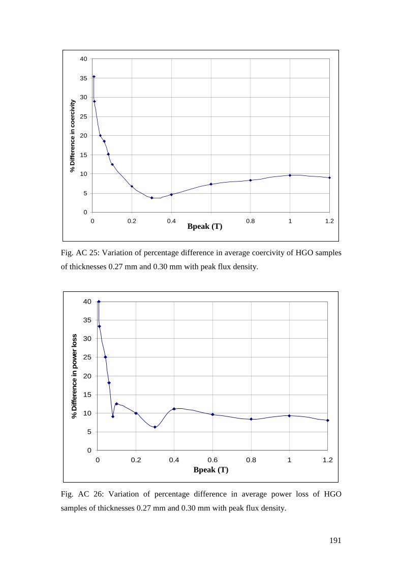
191

0

5

10

15

20

25

30

35

40

0 0.2 0.4 0.6 0.8 1 1.2

B(T)

% D

iffer

ence

in c

oer

civi

ty

Fig. AC 25: Variation of percentage difference in average coercivity of HGO samples


0

5

10

15

20

25

30

35

40

0 0.2 0.4 0.6 0.8 1 1.2

B(T)

% D

iffer

ence

in p

ow

er lo

ss

Fig. AC 26: Variation of percentage difference in average power loss of HGO

samples of thicknesses 0.27 mm and 0.30 mm with peak flux density.

Bpeak (T)

Bpeak (T)

192

APPENDIX D LIST OF PUBLICATIONS

193

Publications

1. Nkwachukwu Chukwuchekwa, Anthony Moses and Phil Anderson, Barkhausen

noise in 3% Si-Fe at 50 Hz, Journal of Electrical Engineering, Vol 61. No 7/s, 69-72,

2010, ISBN/ISSN: 1335-3632.

2. Moses A. J., Anderson P. I., Chukwuchekwa N., Hall J P, Williams P I, Xu X T,

Analysis of magnetic fields on the surface of grain oriented electrical steel,

Measurements 2011, Proceedings of the 8th International Conference, pp. 106-110

Smolenice, Slovakia,

3. Nkwachukwu Chukwuchekwa, Anthony J. Moses and Phil Anderson, Study of

the effects of surface coating on magnetic Barkhausen noise in grain-oriented

electrical steel, IEEE Transactions on Magnetics, Vol. 48, No. 4, April 2012.

4. Nkwachukwu Chukwuchekwa, Anthony J. Moses and Phil Anderson,

Investigation of the effects of strips thickness and grain size on AC magnetic

Barkhausen noise of grain-oriented electrical steel, Przeglad Elektrotechniczny

(Electrical Review). ACCEPTED FOR PUBLICATION .

5. Nkwachukwu Chukwuchekwa, Anthony J. Moses and Phil Anderson, Effects of

Strip Thickness and Silicon Content on Magnetic Barkhausen Noise of Non-oriented

Electrical Steel at 50 Hz, International Journal of Applied Electromagnetics and

Mechanics, ACCEPTED FOR PUBLICATION .

194

Conference Presentations

1. Nkwachukwu Chukwuchekwa, Anthony Moses and Phil Anderson, Barkhausen

noise in grain-oriented 3% Si-Fe at 50 Hz, Magnetic Measurement Conference, 12-15

September, 2010, Prague, Czech Republic ORAL PRESENTATION.

2. Moses A J, Anderson P I, Chukwuchekwa N, Hall J P, Williams P I, Xu X T,

Analysis of magnetic fields on the surface of grain oriented electrical steel,

Measurement 2011 Conference. 27-30 April, 2011, Smolenice Castle, Slovakia.

ORAL PRESENTATION .

3. Nkwachukwu Chukwuchekwa, Anthony J. Moses and Phil Anderson, Effects of

sample thickness and silicon content on Barkhausen noise of Non-oriented electrical

steel at 50 Hz, 15th International Symposium on Applied Electromagnetics and

Mechanics, 7-9 September 2011,Napoli, Italy. ORAL PRESENTATION .

4. Nkwachukwu Chukwuchekwa, Anthony Moses, Phil Anderson and Yevgen

Melikhov, Barkhausen noise technique for non destructive evaluation of grain and

non grain oriented electrical steels, Universal Network of Magnetic Non Destructive

Evaluation (UNMNDE), 24 September 2011, Kos Island, Greece. ORAL

PRESENTATION.

5. Nkwachukwu Chukwuchekwa, Anthony J. Moses and Phil Anderson, Study of

the effects of surface coating on magnetic Barkhausen noise in grain-oriented

electrical steel , 20th Soft Magnetic Materials(SMM) Conference, 18-22 September

2011, Kos Island, Greece. POSTER PRESENTATION.

6. Nkwachukwu Chukwuchekwa, Anthony J. Moses and Phil Anderson,

Investigation of the effects of strips thickness and grain size on AC magnetic

Barkhausen noise of grain-oriented electrical steel, X Symposium on Magnetic

Measurements, 17-19 October 2011, Warsaw, Poland. ORAL PRESENTATION .

Documents

Investigation of Magnetic Properties and Barkhausen … · 2.12 Classical eddy current loss 18 2.13 Anomalous loss 19 ... 5.5.2 The Kerr magneto-optic technique 63 5.6 Uncertainty