Investigation of electronic and magnetic structure of ... › bitstream › urn:nbn:de:gb… · each orientation, there exists an overall magnetic moment. There are also enforced

Investigation of electronic and magnetic structure of advanced magnetic materials

A thesis presented to

Fachbereich Physik Faculty of Physics Universität Osnabrück Babes-Bolyai University

by

Vasile REDNIC

Scientific supervisors: Prof. Dr. Manfred NEUMANN Prof. Dr. Marin COLDEA

Osnabrück January 2010

i

Contents

Introduction .......................................................................................................................................1

1. Theoretical Considerations ....................................................................................................................... 3

1.1 General issues of magnetism ............................................................................................................... 3 1.1.1 The origin of atomic moments ........................................................................................................... 3 1.1.2 Classes of magnetic materials ............................................................................................................ 6

1.2 Magnetic properties of metallic systems ............................................................................................ 9 1.2.1 Localized moments in solids .............................................................................................................. 9 1.2.2 Itinerant-electron magnetism ........................................................................................................... 12 1.2.3 Local moments in metals ................................................................................................................. 16 1.2.4 Self-Consistent Renormalization (SCR) Theory of spin fluctuations of ferromagnetic metals………………………………………………………………………………………….25

1.3 Photoelectron Spectroscopy .............................................................................................................. 26 1.3.1. Physical principles of the technique ................................................................................................ 27 1.3.2 Theory of photoelectron spectroscopy ............................................................................................. 29 1.3.3 Photoelectron spectroscopy models ................................................................................................. 31 1.3.4 Spectral Characteristics .................................................................................................................... 32

2. Preparation and Characterization techniques ...................................................................................... 40

2.1 Sample preparation ........................................................................................................................... 40

2.2 Structure analysis ............................................................................................................................... 40

2.3 Magnetic measurements .................................................................................................................... 42 2.3.1 Vibrating sample magnetometer ...................................................................................................... 42 2.3.2 SQUID magnetometer .................................................................................................................. 44 2.3.3 Weiss balance ................................................................................................................................... 45

2.4 X- ray photoelectron spectroscopy ................................................................................................... 47

2.5 Electronic structure calculations ...................................................................................................... 50

3. Electronic structure and magnetic properties of Mn1-xAlxNi3 alloys ................................................... 52

3.1 Structural characterization ............................................................................................................... 53

3.2 XPS spectra ......................................................................................................................................... 54

3.3 Magnetic measurements .................................................................................................................... 58

3.4 Electronic structure calculations ...................................................................................................... 63

3.5 Conclusions ......................................................................................................................................... 68

4. Electronic structure and magnetic properties of Mn1-xAlxNi alloys .................................................... 70

ii


4.2 XPS spectra ......................................................................................................................................... 72


4.4 Conclusions ......................................................................................................................................... 86

5. Electronic structure and magnetic properties of Ni1-xMnxAl alloys .................................................... 87


5.2 XPS spectra ......................................................................................................................................... 89


5.4 Conclusions ........................................................................................................................................ .96

6. Crystallographic and electronic structure of Ni0.7-xAlxMn0.3 alloys ................................................. …98


6.2 XPS spectra ....................................................................................................................................... 100

6.3 Magnetic measurements .................................................................................................................. 104

6.4 Conclusions ....................................................................................................................................... 107

Summary ........................................................................................................................................109

References ............................................................................................................................................... 111 List of Figures ......................................................................................................................................... 116 List of Tables .......................................................................................................................................... 118

List of Publications .................................................................................................................................... 119

List of Conference Contributions ............................................................................................................. 120

Acknowledgements .................................................................................................................................... 122

1

Introduction

The problem of local moments confined to the transition metals (T) sites, i.e., localized

behaviour in some aspects of itinerant electrons, is one of the most important issues in the

physics of the magnetic alloys and intermetallic compounds. It was found experimentally that

under certain conditions the magnetic moment of a transition metal remains localized when

solute in another transition metal. The condition for the existence of the local moment at the T

site is πΔ / U < 1, where Δ is the width of the d states (corresponds to the virtual bound states in

the Friedel’s model) and U is the Coulomb correlation energy between d electrons.

The 3d band width Δ = Z1/2Jh depends on the number of near-neighbours Z with d orbitals

and the hopping integral John, which is very sensitive to the distance between the atoms. On the

other hand, the strength and the sign of the interaction between the neighbouring local moments

are determined by the occupation fraction of d-orbitals and the orientation of these orbitals in the

lattice. By alloying with other elements, the vicinity of the transition metal atom is changing.

This leads to structural modifications with remarkable variations in the electronic structure and

magnetic properties of the parent compound.

The understanding and prediction of the properties of mater at atomic level represents

one of the great achievements of the last years in science. In this content, the advantage of

photoelectron spectroscopy, in the study of electronic structure and properties of matter is due to

progress in both, experimental and in relevant theory. Photoemission techniques have been

developed sufficiently to become a major tool for the experimental studies of solids. These

techniques are also attractive for the study of changes in, or destruction of, crystalline order.

The fine details of the relationship between the electronic structure and the magnetic

properties of matter represent a state of the art challenge in the solid state physics. The link is

evident even from a didactic approach: electrons are the ’carriers’ of spin magnetic moments and

their movement around nucleus gives rise to orbital momentum i.e. orbital contribution to the

magnetic moments. From a more sophisticated point of view, the information on the electronic

structure turns up to be essential for the understanding of magnetic behavior.

The XPS spectra give information on the electrons binding energies, the valence band

and the density of states at the Fermi level, the hybridization between orbitals, the ions valence

states and the charge transfer between the elements. The energy position and the width of the

valence band, the comparison between the valence band and the calculated band structure, the

2

splitting of the 3s core level, the presence of the satellite structures to the valence band and 2p

core levels give information on the localization degree of the 3d electrons, the occupation of the

3d band, the spin and valence fluctuations effects, which are the basic elements in explaining the

magnetic properties of metallic systems based on 3d elements.

In the present study the ternary system Al-Mn-Ni was chosen because the following reasons:

• Manganese is particularly interesting because according to Hund’s rule the magnetic

moment of the free atom can have the maximum value of 5 μB. The antiferromagnetic

alloys formed by Mn with nickel, palladium, and platinum have high Néel temperatures,

which makes them very promising materials for practical applications, such as pinning

layers of GMR and TMR devices.

• Nickel metal is a ferromagnet having a magnetic moment of 0.6 μB/Ni. By alloying with

Al, the Ni 3d-Al 3sp hybridization leads to a partial (AlNi3) or complete (AlNi) filling of

Ni 3d band depending on Al concentration and distances between Al and Ni atoms.

• By varying the concentration of the elements the first vicinity of transition metal atoms

and the distance between them is different, which leads to important changes in the

crystallographic and electronic structure with remarkable effects on the magnetic

properties of Mn-Ni-Al alloys and compounds.

The aim of this thesis is to study the changes in the crystallographic, electronic and

magnetic structure of the Al-Mn-Ni ternary metallic system by modifying the concentration of

the constituent elements.

The thesis is organized in 6 Chapters, followed by the summary. Chapter 1 contains a

brief theoretical introduction into the magnetism of metallic systems, as well the principles of X-

ray photoelectron spectroscopy, which is the main technique used to investigate the electronic

structure of the intermetallic alloys and compounds. The sample preparation details and all the

experimental techniques employed in the characterization of the systems are described in

Chapter 2. The next 4 Chapters contain the experimental results for Mn1-xAlxNi3, Mn1-xAlxNi,

Ni1-xMnxAl, and Ni0.7-xAlxMn0.3 systems. The structural, electronic and magnetic properties of

the alloys and compounds are investigated by X-ray diffraction, X-ray photoelectron

spectroscopy, band structure calculations, magnetization and magnetic susceptibility

measurements.

3

Chapter 1 Theoretical considerations

1.1 General issues of magnetism

All materials have an inherent magnetic character arising from the movements of their

electrons. Since dynamic electric fields induce a magnetic field, the orbit of electrons, which

creates atomic current loops, results in magnetic fields. An external magnetic field will cause

these atomic magnetic fields to align so that they oppose the external field. This is the only

magnetic effect that arises from electron pairs. If a material exhibits only this effect in an applied

field it is known as a diamagnetic material.

Magnetic properties other than diamagnetism, which is present in all substances, arise

from the interactions of unpaired electrons. These properties are traditionally found in transition

metals, lanthanides, and their compounds due to the unpaired d and f electrons on the metal.

There are three general types of magnetic behaviors: paramagnetism, in which the unpaired

electrons are randomly arranged, ferromagnetism, in which the unpaired electrons are all aligned,

and antiferromagnetism, in which the unpaired electrons line up opposite of one another.

Ferromagnetic materials have an overall magnetic moment, whereas antiferromagnetic materials

have a magnetic moment of zero. A compound is defined as being ferrimagnetic if the electron

spins are orientated antiparrallel to one another but, due to an inequality in the number of spins in

each orientation, there exists an overall magnetic moment. There are also enforced ferromagnetic

substances (called spin-glass-like) in which antiferromagnetic materials have pockets of aligned

spins.

1.1.1 The origin of atomic moments

At the atomic scale, magnetism comes from the orbital and spin electronic motions. The

nucleus can also carry a small magnetic moment, but it is insignificantly small compared to that

of electrons, and it does not affect the gross magnetic properties.

Quantum mechanics gives a fixed energy level to each electron which can be defined by

a unique set of quantum numbers:

1. The total or principal quantum number n with integral values 1, 2, 3,… determines the size of

the orbit and defines its energy. Electrons in orbits with n=1, 2, 3,… are referred to as

occupying K, L, M,… shells, respectively.

4

2. The orbital angular momentum quantum number l describes the angular momentum of the

orbital motion. For a given value of l, the angular momentum of an electron due to its orbital

motion equals )1( +llh . The number l can take one of the integral values 0, 1, 2,…, n-1. The

electrons with l = 0, 1, 2, 3,… are referred to as s, p, d, f, … electrons, respectively.

3. The magnetic momentum quantum number ml describes the component of the orbital angular

momentum l along a particular direction. For a given l: ml= l, l-1,…, 0,…,-l+1,-l

4. The spin quantum number ms describe the component of the electron spin along a particular

direction, usually the direction of the applied field. The electron spin s is the intrinsic angular

momentum corresponding with the rotation (or spinning) of each electron about an internal

axis. The allowed values of ms are ±1/2.

According to the Pauli Exclusion Principle, each electron occupies a different energy

level (or quantum state), thus the states of two electrons are characterized by different sets of

quantum numbers n, l, ml, and ms.

The motion of the electron around the nucleus may be considered as a current flowing in

a wire having no resistance, which coincides with the electron orbit. The corresponding magnetic

effects can be than derived by considering the equivalent magnetic shell. An electron with an

orbital angular momentum ħl has an associated magnetic moment:

llme

Bl

rrh

r μμ −=−=2

(1.1)

where μB is the Bohr magneton: m

eB 2

h=μ (1.2)

The absolute value of the magnetic moment is given by:

)1( += llBl μμr (1.3)

The situation is different for the spin angular momentum. In this case, the associated magnetic

moment is:

sgsme

g Beesrr

hr μμ −=−=

2 (1.4)

where ge (=2.002290716) is the spectroscopic splitting factor.

The magnetic moment of a free atom (or ion) is the sum of the moments of all electrons.

When describing the atomic origin of magnetism, one has to consider the orbital and spin

motions of all electrons as well as the interactions between them. The maximum number of

electrons occupying a given shell is:

5

∑−

=

=+1

0

22)12(2n

lnl (1.5)

The total orbital angular momentum and total spin angular momentum of a given atom are

defined as:

∑=i

ilLrr

(1.6)

and respectively: ∑=i

isS rr (1.7)

where the summation extends over all electrons. The summation over a complete shell is zero, so

only the incomplete shells contribute effectively to the total angular momentum. The resulted Sr

and Lr

are coupled through the spin-orbit interaction to form the resultant total angular

momentum Jr

:

SLJrrr

+= (1.8)

For all but the heaviest atoms the ground state of a free atom with an unfilled shell is determined

by three empirical rules known as Hund’s rules:

1. The ground state will have the largest spin S that is consistent with the Pauli Exclusion

Principle.

2. The ground state will have the largest total orbital angular momentum L that is consistent

with both the first rule and the exclusion principle.

3. This rule determines the value of the overall total angular momentum number J, which

can lie between SL − and SL + . The ( ) ( )1212 +×+ SL possible states have different

energies that are determined by interactions of the form SLrr

⋅λ which is known as Russel-

Saunders coupling. The factor λ is positive for shells that are less than half filled, and

negative for shells that are more than half filled. Thus J is given by the number N of

electrons:

SLJ −= for N ≤ 2l+1 and SLJ += for N ≥ 2l+1

When J has a non-zero value, the atom or ion has a magnetic moment:

Jg B

rr μμ −= (1.9)

with the absolute value:

)1( += JJg Bμμ (1.10)

where g is the Landé spectroscopic factor and is approximately:

6

)1(2)1()1()1(1

++−+++

+≈JJ

LLSSJJg (1.11)

In most cases, the energy separation between the ground-state level and the other levels

are large compared to kT. For describing the magnetic properties of the ions at 0K, it is therefore

sufficient to consider only the ground state characterized by the angular momentum quantum

number J.

Two series of elements play a fundamental role in magnetism: the 3d transition elements

and the 4f rare earths. These two series are important because the unfilled shells are not the outer

shells and in solids the 3d (respectively 4f) shell can remain unfilled, leading to magnetism. In

the case of the 4d and 5d series of elements, the magnetism is generally very weak. This is

because the 4d and 5d shells are rather delocalized, allowing the participation of these electrons

to the conduction band.

1.1.2 Classes of magnetic materials

Diamagnetism

Diamagnetism is a fundamental property of all matter, although it is usually very weak. It

can be regarded as originating from the shielding currents induced by an applied field in the

filled electron shells of ions. These currents are equivalent to an induced moment present on each

of the atoms. The diamagnetism is a consequence of Lenz’s law stating that if the magnetic flux

enclosed by a current loop is changed by the application of a magnetic field, a current is induced

in such a direction that the corresponding magnetic field opposes the applied field. The magnetic

susceptibility of diamagnetic materials is negative and has no temperature dependence.

Paramagnetism

In the case of paramagnetic materials, some of the atoms carry intrinsic magnetic

moments due to unpaired electrons in partially field orbitals, but the individual magnetic

moments do not interact with each another. The magnetization is zero in the absence of an

external magnetic field, like for diamagnetic materials. The presence of an external magnetic

field leads to a partial alignment of the atomic magnetic moments in the direction of the field,

resulting in a net positive magnetization and positive susceptibility. The efficiency of the field is

opposed by the thermal effects which favour disorder of magnetic moments and tend to decrease

the susceptibility. This results in a temperature dependent susceptibility, known as Curie’s law:

TC

=χ (1.12)

7

At normal temperatures and in moderate fields, the paramagnetic susceptibility is small, but

larger than the diamagnetic contribution. Curie’s law states that if the reciprocal values of the

magnetic susceptibility, measured at various temperatures, are plotted versus the corresponding

temperatures, one finds a straight line passing through the origin. The Curie constant can be

estimated from the slope of this line and hence a value for the effective moment.

Ferromagnetism

Ferromagnetic materials have a non vanishing magnetic moment, or spontaneous

magnetization, even in the absence of a magnetic field. Unlike paramagnetic materials, the

atomic moments in these materials exhibit very strong interactions. These interactions are

produced by electronic exchange forces and result in a parallel alignment of atomic moments.

The exchange force is a quantum mechanical phenomenon due to the relative orientation of the

spins of two electrons. The elements Fe, Ni, and Co and many of their alloys are typical

ferromagnetic materials. Two distinct characteristics of ferromagnetic materials are their

spontaneous magnetization and the existence of magnetic ordering temperature, called Curie

temperature. The spontaneous magnetization is the net magnetization that exists inside a

uniformly magnetized microscopic volume in the absence of a field. The magnitude of this

magnetization, at 0K, is dependent on the spin magnetic moments of electrons. The magnetic

ordering competes with thermal disorder effects and each material is characterized by a critical

temperature (Curie temperature), which is a measure of the strength of magnetic interactions and

is an intrinsic property of the material.

M

χ-1

TC θ

M~(1+αT3/2)

M~(1-T/TC)1/3

T0

M

χ-1

TC θ

M~(1+αT3/2)

M~(1-T/TC)1/3

T0

Fig. 1.1. The temperature dependence of the spontaneous magnetization M (T<TC) and

magnetic susceptibility )( CTT >χ for a ferromagnetic system

At temperatures above the Curie temperature the thermal effects dominate and the

material has a paramagnetic behaviour; below this temperature the magnetic interactions

dominate and the material is magnetically ordered. Above the Curie temperature the magnetic

susceptibility obeys the Curie-Weiss law:

8

pTCθ

χ−

= (1.13)

where θp>0 is called the asymptotic or paramagnetic Curie temperature and differs from the

Curie temperature due to the thermal fluctuations.

In addition to the Curie temperature and saturation magnetization, ferromagnets can

retain a memory of an applied field once it is removed. This behaviour is called hysteresis and a

plot of the variation of magnetization with magnetic field is called a hysteresis loop.

Antiferromagnetism

In the case of antiferromagnets, although there is no net total moment in the absence of

the field, the magnetic interactions favour an antiparallel orientation of neighbouring moments.

In a simple antiferromagnet, magnetic atoms can be divided into two sublattices with their

magnetizations equal but antiparallel. The net magnetization is then zero at any temperature.

The clue to antiferromagnetism is the behaviour of susceptibility above a critical temperature,

called the Néel temperature (TN). Above TN, the susceptibility obeys the Curie-Weiss law for

paramagnets but with a negative intercept indicating negative exchange interactions.

TN T

χ

0

χ-1

θ TN T

χ

0

χ-1

θ

Fig. 1.2. The temperature dependence of the magnetic susceptibility for an antiferromagnet

Slight deviations from ideal antiferromagnetism can exist if the anti-parallelism is not exact. If

neighbouring spins are slightly tilted (<1°) or canted, a very small net magnetization can be

produced. This is called canted antiferromagnetism and hematite is a well known example.

Canted antiferromagnets exhibit many of the typical magnetic characteristics of ferromagnets

and ferrimagnets (e.g., hysteresis, Curie temperature).

Ferrimagnetism

A ferrimagnet is an antiferromagnet in which the different sublattice magnetizations are

not equal, which results in a net magnetic moment. This requires non equivalent magnetic

sublattices and/or atoms. Ferrimagnetism is therefore similar to ferromagnetism. It exhibits all

the hallmarks of ferromagnetic behaviour spontaneous magnetization, Curie temperatures, and

9

hysteresis. However, ferromagnets and ferrimagnets have very different magnetic ordering. The

temperature dependence of the magnetization in ferrimagnetic compounds is determined by the

magnitude and sign of the coupling constants that describe the magnetic coupling between the

different sublattices and between two moments residing on the same magnetic sublattice. Above

the Curie temperature the reciprocal susceptibility is given by the Néel hyperbolic law:

θσ

χχ −−+=

TCT

0

11 (1.14)

where C is the mean value of the Curie constant and χ0, σ and θ are constants that depend on the

nature of the sublattices present in the system.

χ-1

TCθ T0

M

MA

MB

M

MA

MB

M

MA

MBT T T

χ-1

TCθ T0

χ-1

TCθ T0

M

MA

MB

M

MA

MB

M

MA

MBT T T

Fig. 1.3. The temperature dependence of the spontaneous magnetization M (T<TC)

(several cases are presented) and magnetic susceptibility χ (T>TC) for a ferrimagnetic

system consisting of two sublattices A and B

1.2 Magnetic properties of metallic systems

There are several models in magnetism, but none that fully describes the magnetic

behaviour for magnetically ordered materials. Although the molecular field theory gives an

intuitive description for the most important physic properties of ferromagnetic materials

(temperature dependence of spontaneous magnetization, specific heat and magnetic susceptibility

behaviour at high temperatures), it fails to describe the low temperatures and critical regions. At

very low temperatures the experimental results are best described by the spin waves theory.

1.2.1 Localized moments in solids

The magnetic interaction between localized moments, the magnetic coupling, determines

the behaviour of a compound when placed in a magnetic field and may favor magnetic ordering.

The magnetic coupling is usually described in terms of a model spin Hamiltonian, most often the

Heisenberg Hamiltonian:

∑−=ji

jiij SSJH,

rr (1.15)

10

where i, j can be restricted to run over all nearest neighbour or next nearest neighbour pairs of

magnetic moments on account of the fact that the magnetic interaction is weak and decreases

exponentially with distance. Positive values of the Heisenberg coupling constant J correspond to

ferromagnetic coupling, negative ones to antiferromagnetic coupling. In 3d based

materials KJij32 1010 ÷≈ . A spin operator of this form was first deduced from the Heitler-

London results by Dirac [1] and first extensively applied in the theory of magnetism by Van

Vleck [2]. The universal use of the name Heisenberg Hamiltonian acknowledges his original

discussion of the quantum mechanical concept of electron exchange and the introduction of the

term exchange integral in his theoretical work on the helium atom [3]. A conceptually similar

but not at all identical term appears in the work of Heitler and London to express the difference

in energy between the singlet and triplet states in the hydrogen molecule.

When the magnetic orbitals of two neighbouring atoms are sufficiently extended to

produce a direct overlap, there is an effective interaction between the spins of these atoms, called

direct exchange. The origin of the exchange interaction is in the different energies for the

parallel and antiparallel spin states as a result of the Pauli principle. This direct exchange, which

occurs in 3d intermetallic compounds, is the largest interatomic interaction and it is, in particular,

responsible for the high ordering temperatures found in the ferromagnets used for most

technological applications. The Slater-Néel curve illustrates the variation of this interaction as a

function of interatomic distance and magnetic shell radius.

Fig. 1.4. Slater-Néel curve (d=distance between two atoms, r=magnetic shell radius)

When magnetic orbitals of two neighbouring atoms are too localized to overlap, as in the

case for the 4f series, the exchange process can occur through conduction electrons if the system

is metallic. This leads to the RKKY indirect exchange interaction. If there are no conduction

electrons, as in ceramics where magnetic atoms are separated by non-magnetic atoms like

oxygen, the external electrons of the latter participate in covalent binding and mediate the

11

exchange interaction. This is the superexchange interaction. The term superexchange was

introduced by Kramers [4] in 1934 in an early attempt to explain the magnetic interaction in anti-

ferromagnetic ionic solids. The distance between the transition metal ions is generally far too

large for direct magnetic interactions, as occur in metals, to be of any significance. Since the

metal ions always have negative ions as nearest neighbours he proposed that these anions played

an intermediary role in the interaction mechanism. A more elaborate and successful evaluation

was carried out in 1959 by Anderson [5].

The Molecular Field Model

Pierre Weiss postulated the presence of a molecular field in his phenomenological theory

of ferromagnetism in 1907 [6], long before its quantum-mechanical origin was known. The

model proposed by Weiss is based on the powerful assumption that the fluctuations of molecular

field with time and the dependence on the instantaneous values of the magnetic moments can be

neglected. The origin of the Weiss molecular field was attributed by Heisenberg [7] to the

quantum-mechanical exchange interaction between neighbouring atoms, usually written:

∑<

−=ji

jiijexch SSJHrr

2 (1.16)

where the summation extends over all spin pairs in the crystal lattice. The exchange constant Jij

depends, amongst other things, on the distance between the two atoms i and j considered. In most

cases, it is sufficient to consider only the exchange interaction between spins on nearest-

neighbour atoms. By considering Z magnetic nearest-neighbour atoms surrounding a given

magnetic atom, the exchange Hamiltonian becomes:

SSZJH nnexch

rr⋅−= 2 (1.17)

where Sr

is the average spin of the nearest-neighbour atoms. This relation can be rewritten:

( ) JJgZJH nnexch

rr⋅−−= 212 (1.18)

The atomic moment is related to the angular momentum by (Eq. 1.9), resulting in:

( )m

B

nnexch H

ggZJ

Hrr

rr

μμμ

μμ022

212−=

⋅−−= (1.19)

where:

( )22

212

B

nnm g

gZJH

μμrr −

= (1.20)

12

can be regarded as an effective field, the so-called molecular field, produced by the average

moment μr of the Z nearest-neighbour atoms. If all the magnetic moments are identical, the

magnetization of the system can be written μrr

NM = and in consequence mHr

is proportional

to the magnetization:

MNH Wm

rr= (1.21)

The constant NW is called the molecular-field constant or the Weiss-field constant.

In the Weiss molecular filed theory the Curie temperature is given by:

B

BWC k

JJgNNT

3)1( 22

0 μμ += (1.22)

and the magnetic susceptibility above CT is given by:

)(3)1( 22

0

CB

B

TTkJJgN−+

=μμ

χ (1.23)

Heisenberg assumed that the exchange integral between neighbouring atoms is positive

and of appropriate order of magnitude. Subsequent attempts to calculate J for ferromagnetic

transition metals from realistic atomic orbitals have failed to explain the sign and magnitude

of J . In fact, the molecular field theory gives a grossly inadequate picture of the critical region,

fails to predict spin waves at low temperatures, and even at high temperatures reproduces

without error only the leading correction to Curie’s law. Nevertheless the theory has been widely

used and quoted and when confronted with a new situation (e.g., a particular complicated

arrangement of spins on a crystal structure with several types of coupling) it probably offers the

simplest rough way of sorting out the types of structures expected to arise. Also the molecular

field theory is sometimes taken as starting point for more sophisticated calculations.

The Heisenberg model is actually justified when well-defined local atomic moments

exist, like in the case of magnetic insulators and in the majority of rare-earth metals. In the

former, the mechanism of exchange interaction is the superexchange which is usually

antiferromagnetic, while in the latter indirect exchange interaction via the conduction electrons

dominates.

1.2.2 Itinerant-electron magnetism

Opposite to the localized model is the itinerant (or band) model which considers that each

magnetic carrier (electron or hole) is itinerant through the solid. In this case, the unpaired

electrons responsible for the magnetic moment are no longer localized and accommodated in

13

energy levels belonging exclusively to a given atom, but move in the potential of other electrons

and ions, and the corresponding atomic levels form energy bands. The extent of the broadening

of the energy bands depends on the interatomic separation between the atoms. The ordered

magnetic states, stabilized by electron-electron interactions, are characterized by the difference

of the number of electrons (or holes) with up and down spins. The most prominent examples of

itinerant-electron systems are metallic systems based on 3d transition elements, with the 3d

electrons responsible for the magnetic properties, where the unfilled d shell is rather extended.

The Stoner Model

The simplest model of itinerant-electron magnetism is the Stoner model [8], which has

mainly been used to account for the existence of ferromagnetism in itinerant systems. If the

relative gain in the exchange interaction (the interaction of electrons via Pauli's exclusionary

principle) is larger than the loss in kinetic energy, the spin up and spin down electron bands will

split spontaneously. In the Stoner band model, the energies of the spin up and down electron

bands are:

nn

IkEkE

nn

IkEkE

↓↓

↑↑

−=

−=

)()(

)()(

rr

rr

(1.24)

where ( )kEr

is the energy of the metal before exchange effects are included, ↑n and ↓n represent

the number of electrons with spin up and spin down, and n is the number of electrons in the

system (N=n↑+n↓). The Stoner parameter I describes the energy change due to electron spin

correlations. The relative difference between the number of electrons occupying the spin up and

spin down bands is:

nnn

R ↓↑ −= (1.25)

which is proportional to the magnetization of the system.

In consequence:

2)(~)(

2)(~)(

IRkEkE

IRkEkE

+=

−=

↓

↑

rr

rr

(1.26)

where: nnn

IkEkE2

)()(~ ↓↑ +−=rr

(1.27)

The energy separation between the two bands is independent of the wave vector of an electron.

14

We can evaluate R using the Fermi-Dirac statistics, where:

∑∑+⎟

⎟⎠

⎞⎜⎜⎝

⎛ −==

k

B

Fk

TkEkE

kfnrr

rr

1)(exp

1)( (1.28)

which gives ∑⎥⎥⎥⎥⎥

⎦

⎤

⎢⎢⎢⎢⎢

⎣

⎡

+⎟⎟⎠

⎞⎜⎜⎝

⎛ −+−

+⎟⎟⎠

⎞⎜⎜⎝

⎛ −−=

k

B

F

B

F

TkEIRkE

TkEIRkEn

Rr

rr

12/)(~exp

1

12/)(~exp

11 (1.29)

Eq. (1.29) can have real solutions, which means that the system has a magnetic moment

in the absence of an external magnetic field, and therefore is ferromagnetic. In order to find the

condition for the existence of magnetic moments in the system, the following approximation is

used:

)(2!3

2)(22

3

xfxxxfxxfxxf ′′′⎟⎠⎞

⎜⎝⎛ Δ−Δ′−=⎟

⎠⎞

⎜⎝⎛ Δ

+−⎟⎠⎞

⎜⎝⎛ Δ

− (1.30)

which leads to:

33

3

)()(~)(1

241

)(~)(1 IR

kEkf

nIR

kEkf

nR

kk∑∑

∂∂

−∂∂

−= r

r

r

r

(1.31)

If R>0 the band is exchange split, which corresponds to ferromagnetism. Therefore the condition

for the stability of a ferromagnetic state is:

∑ >∂∂

−−k kE

kfnI 0

)(~)(1 r

r

(1.32)

Considering that around 0K: )~(~ FEEEf

−=∂∂

− δ , we can write:

∑ ∫ ∫ =−=⎟⎠⎞

⎜⎝⎛∂∂

=∂∂

kFF EN

nVEEkd

nV

Efkd

nV

kEkf

n)(

21)~(1

)2(~)2()(~)(1

33 δππ

rrr

r

(1.33)

Thus a ferromagnetic state is realized for:

1)( >FEIN (1.34)

where )( FEN is the density of states at the Fermi energy per spin and volume.

The later condition is the Stoner criterion for ferromagnetism.

The conditions favouring magnetic moments in metallic systems are obviously: a large

value of the exchange energy, but also a large density of state at the Fermi level. The density of

states of the s and p electron bands is considerably smaller than that of the d band, which

15

explains why band magnetism is restricted to elements that have a partially empty d band.

However, not all of the d transition elements show band ferromagnetism, as presented in Fig. 1.5.

For instance, in the 4d metal Pd, the Stoner

criterion is not met, although it comes very close to

it. The only pure d metals that show band

ferromagnetism under normal conditions are Fe, Co

and Ni.

Two situations have to be considered in the

case of itinerant-electron magnetism:

- if both the spin up and spin down bands are not

completely filled up, the compound is a weak

ferromagnet; this is the case for Fe metal

- if the spin up band is completely full, the

compound is a strong ferromagnet; this is the case

for Ni and Co metals

These terms are only definition and they do

not do not imply that the spontaneous moments per

3d atom or the magnetic ordering temperatures are higher in the former case than in the latter.

Indeed, n Fe the magnetization is 2.4µB/Fe whereas in Co and Ni it is 1.9 and 0.6 respectively.

The magnetization of the system at T≈0K is:

BEIN

ENVnM

F

FB )(1

)(2 2

−= μ (1.35)

When IN(EF) is barely larger than 1, the Stoner criterion is fulfilled but the magnetization is

weak and we have the so-called very weak itinerant ferromagnetism.

The magnetic susceptibility is given by:

)(10

FEIN−=

χχ (1.36)

where 0χ is the Pauli susceptibility of free electrons. This is referred to as the Stoner

enhancement of the susceptibility.

This itinerant electron model is consistent with the observed magnetizations per atom of

Fe, Co, Ni, which are not integral multiples of the Bohr magneton per 3d atom. However, the

Stoner theory fails to explain the Curie-Weiss magnetic susceptibility observed in almost all

ferromagnets. Calculated Curie temperatures for 3d metals are too high in comparison to the

Fig. 1.5. a) the Stoner parameter, b) the density of states at Fermi level, c) the Stoner criterion [9]

16

observed ones and the calculated anomalous entropy around the Curie temperature is too small to

explain the observed values.

1.2.3 Local moments in metals

Both the localized model and itinerant model fail to fully describe the magnetic

behaviour of magnetic transition metals. It is very clear that d electrons should be treated as

localized electrons in magnetic insulator compounds and as correlated itinerant electrons in

transition metals. Theoretical efforts since the 1950s have been concentrated on finding a way of

reconciling the two mutually opposite pictures into a unified one, taking into account the effect

of electron-electron correlation in the itinerant electron model. There have been two main

directions in this attempt: one was to improve the Stoner theory by considering the electron-

electron correlation, and the other was to start with the study of local moments in metals.

The picture of local moments in metals resolved the controversy over the two models.

Van Vleck [10] discussed the justification of local moments, considering the importance of

electron correlation in narrow d bands. An explicit model describing the local moments in metals

was proposed by Anderson [11] on the basis of the Friedel picture of virtual bound states in

dilute magnetic alloys [12].The Anderson concept of local moments in metals has been quite

important in the development of the theory of ferromagnetic and antiferromagnetic metals. It

may be possible in some cases to regard a metallic ferromagnet as consisting of local moments

associated with the virtual bound states. Although in this case the local moment is not as well

defined as in insulator magnets, an approximate Heisenberg-type picture can be used even in

metals. The interaction between local moments in metals was studied by Alexander an Anderson

[13] and by Moriya [14] on the basis of the Anderson model. Simple rules regarding the sign of

the effective exchange coupling between neighbouring moments were obtained, which will be

discussed later on. These rules and their generalizations for a pair of different atoms were

successfully applied to explain various magnetic structures of numerous ferromagnetic and

antiferromagnetic metals, intermetallic compounds and alloy.

Virtual bound state

The picture of local moments in metals is tied up with the concept of virtual bound states

introduced by Friedel for dilute alloys [12]. Consider a transition metal impurity in a non-

magnetic metallic host. The excess nuclear charge (the charge of the interstitial impurity or the

change in charge if the impurity substitutes an atom in the matrix) displaces locally the mobile

electrons until the displaced charge screens out the new nuclear charge. As the screening should

17

be perfect within the limits of classical physics, its radius should have atomic dimensions. The

effect is a perturbing potential in addition to the periodic potential of the pure matrix at the

impurity position.

Alloys with transitional impurities often exhibit peculiar properties that are related to the

presence of d bound states or virtual bound states. In transition metals the screening occurs on

the impurity atom itself and thus two impurity atoms do not interact even when nearest

neighbours. In Fig. 1.6 is presented the case of a transition metal atom with a spherical potential

(pictured by the dashed curve) that accommodates a d bound state characterized by the quantum

number l. If the perturbing potential reduces the potential of the impurity from the value of the

dashed curve to the actual value corresponding to the continuous curve, the bound state increases

in energy and merges into the conduction band of the host. The interaction of the d electron with

the conduction electrons leads to an admixture or hybridization between the s states of the solute

and the d states of the impurity. As a result there will no longer be a localized bound d state, but

a wave packet of width w localized at the transition element position around E0, producing a

virtual bound state.

Fig.1.6. Real bound state and virtual bound state in energy versus space diagram [12]

The width w of the virtual bound level decreases for increasing l (for l=0 it is so large

that virtual s levels have no physical significance) and for a give l it is roughly proportional to

E0. The width of the virtual d states for transitional impurities in Al is around 4eV, due to the

high Fermi energy, while in Cu matrix is around 2eV, if the conductive electrons are treated as

free. The splitting within the d shell due to the exchange interactions can only occur if the energy

of splitting is larger than the width w of the states. The condition considering Hund’s rule is:

Epw Δ≤ (1.37)

where p is the number of electrons (if less than 5) or holes (otherwise) in the d shell and ΔE is

the average energy gained when two d electrons with antiparallel spins are put with their spins

18

parallel. From atomic spectra ΔE is estimated from 0.6 to 0.7 eV. As p≤5, the exchange splitting

is impossible in Al. For Cu matrix the exchange splitting occurs for p≥3, thus for impurities like

Fe, Mn or Cr, but not for Ni or Co.

The interaction with the conduction electrons can be also regarded as a scattering

problem. Consider an impurity atom embedded in an electron gas. Assuming the impurity

potential to be spherically symmetric around the origin, we have the problem of an electron

scattered by the impurity potential. We are interested in a change in the density of states induced

by the impurity atom. The transition metal atom introduces an excess charge Z, which must be

screened by the same amount of electronic charge, as required by the charge neutrality condition.

The redistribution of the conduction electrons results in a change in density of states in the

energy range ε to ε+dε.

δεεδεεη

πδε

εη

πδ

σ

σ

σ

σ )()12(1)12(1)(,,

Nd

dlk

dkd

dd

lkkNl

l

l

l Δ≡⎟⎠⎞

⎜⎝⎛+=⎟

⎠⎞

⎜⎝⎛⎟⎠⎞

⎜⎝⎛+=Δ ∑∑ (1.38)

where ηlσ is the phase shift for the lth partial wave function of a scattered electron with spin σ.

The total excess electronic charge is obtained by integrating up to the Fermi level and must be

equal to the extra charge of the impurity Z. Thus the following Friedel sum arises:

∑ +=l

Fl ElZ )()12(2 ηπ

(1.39)

where the factor 2 is due to the spin degeneracy.

When an energy level of the impurity atom is close to the energy of an incident electron,

resonance scattering takes place and the phase shift varies very rapidly with energy. For a

transition metal impurity atom the d-wave (l=2) scattering shows this character. This means that

the bound state of the impurity atom, when introduced in a metal, resolves into scattered states

within a relatively small energy range. The change in the density of states due to the d-wave

scattering from an impurity atom is given from the term with l=2 in Eq. (1.38) as:

∑=Δσ

σ

εη

πε

dd

N 22

5)( (1.40)

When this has a fairly sharp peak it is called a virtual bound state.

By taking account of the exchange interaction between d electrons in the impurity atom,

the virtual bound state can split under favourable conditions. The condition may be given by:

1)(2 >Δ FENJ (1.41)

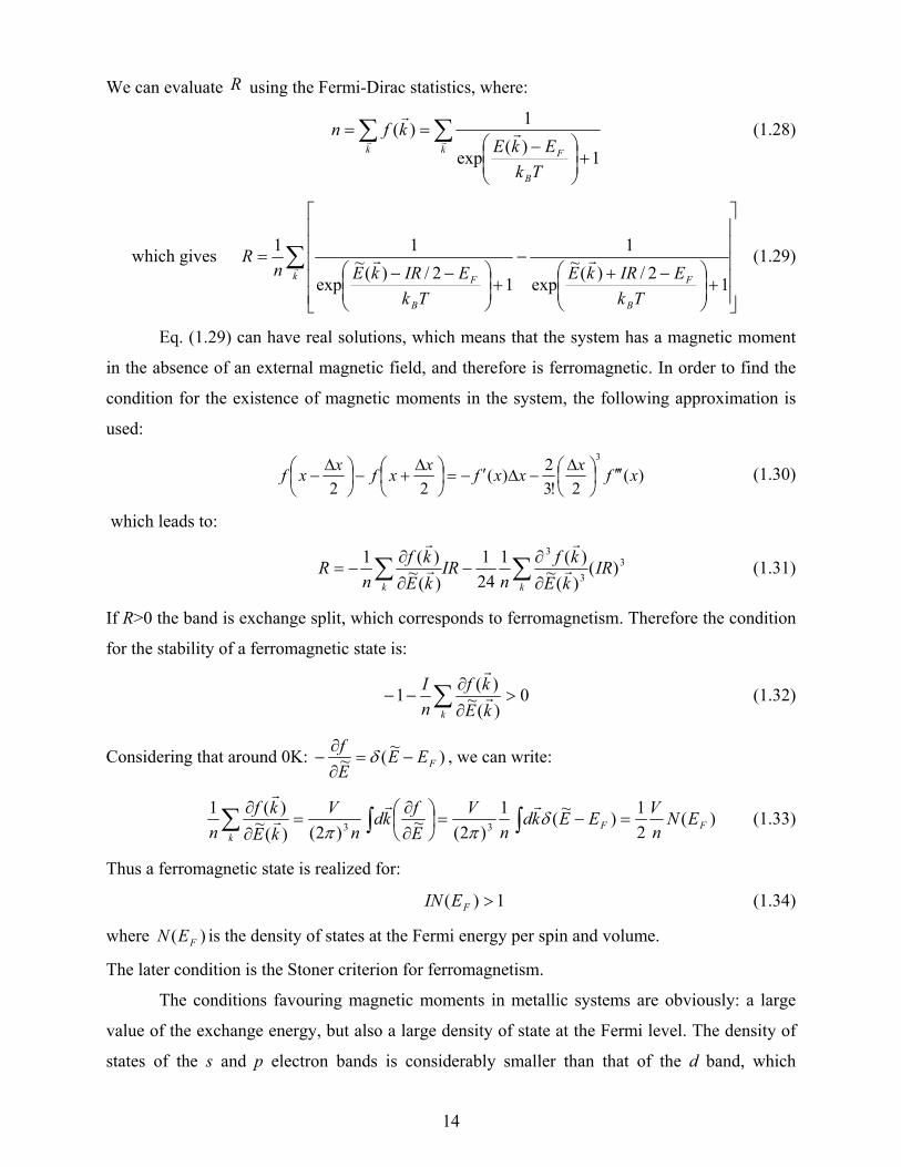
where J is the intra-atomic exchange energy. When there is a local moment of size M, the phase

shifts are derived from:

19

)(25

)(25

22

22

↓↑

↓↑

+=

−=

ηηπ

ηηπ

Z

M (1.42)

By using these relations Friedel gave a systematic explanation of the residual resistivity

due to 3d-metal impurities in Al and Cu. In the former case impurity atoms have no local

moment while in the latter some of them have local moments.

The Anderson Model

The “Anderson model” [11] is the simplest one which provides an electronic mechanism

for the existence of local moments. Assuming that the local moment exists, this means that a d-

shell state φd on the impurity atom of spin up is full and of spin down is empty. Since only a spin

down electron can be added, an electron of spin down will see the repulsion of the extra-spin

electron, while the electrons of spin-up will not. Thus if the unperturbed energy of the spin-up

state is situated at Ed below the Fermi surface, the energy of the spin-down state will be –Ed+U,

where U is the repulsive d-d interaction and must lie above the Fermi level because we assumed

that this state is empty. The effect of covalent admixture of free-electron states with the d states

is to reduce the number of electrons in the spin-up state and to increase the number of the spin-

down state, which leads to a reduction of the total moment. The changes in the number of d

electrons are such as to decrease the difference U between the spin-up and spin-down energies: -

Ed moves up to –Ed+δnU and –Ed+U moves down to –Ed+(1-δn)U. δn depends on the density

of the free ions, the strength of the electron admixture and on the energy difference between up

and down states. If, by a change of one of these parameters, is increase, the energy difference

between decreases. The situation may become completely unstable, resulting in the

disappearance of the local magnetic moment.

In order to deal with the local moment in metals more explicitly, Anderson introduced a

mathematical model, in which he inserted the vital on-site exchange term U, and characterized

the impurity atom by an additional orbital φd, with occupancy ndσ and creation operator +σkc over

and above the free electron states near the Fermi surface of the metal. The Hamiltonian is

expressed by:

sdcorrdf HHHHH +++= 00 (1.43)

H0f is the unperturbed energy of the free electron system in second-quantized notation:

20

σσσ

σσε

kkk

kkkf

ccn

nH

+=

= ∑0

(1.44)

where εk is the energy of the free electron state of momentum k.

The second term is the unperturbed energy of the d states on the impurity atom:

)(0 ↓↑ += dddd nnEH (1.45)

The third term is the repulsive energy among the d functions:

↓↑= ddcorr nUnH (1.46)

The fourth essential part of the Hamiltonian is the s-d interaction term:

∑ ++ +=σ

σσσσ,

)(k

kddkdksd ccccVH (1.47)

where Vdk is the matrix element for the covalent admixture between the impurity state and the

conduction band.

Anderson obtained by Green’s function methods the density distribution of the d state:

22)(1)(

Δ+−Δ

=σ

σ επε

ENd (1.48)

where Δ is the “width parameter” of the virtual state, defined by:

)(2 επ NVav

=Δ (1.49)

and: σσ −+= dd nUEE (1.50)

In Fig. 1.7 are shown the two virtual states in terms of their distributions Ndσ(ε) from Eq. (1.48)

centered around the self-consistent energies Eσ.

Fig.1.7. Density of state distributions in a magnetic state. The arrows indicate the spin up

and spin down. The “humps” at Ed+U<n↓> and Ed+U<n↑> are the virtual d levels of

width 2Δ, for up and down spins, respectively. [11]

21

In order to determine the number of d electrons of a given spin σ, we integrate Eq. (1.48) up to

the Fermi energy EF:

⎟⎠⎞

⎜⎝⎛

Δ−

=Δ+−

Δ= −

∞−∫ FE

dEEd

En

Fσ

σσ π

εεπ

122 cot1

)(1 (1.51)

Thus:

⎟⎟⎠

⎞⎜⎜⎝

⎛

Δ

+−=

⎟⎟⎠

⎞⎜⎜⎝

⎛

Δ

+−=

↑−↓

↓−↑

dFdd

dFdd

nUEEn

nUEEn

1

1

cot1

cot1

π

π (1.52)

To show the possibilities inherent in these equations, Anderson introduced two dimensionless

parameters:

1. Δ

=Uy (the ratio of the Coulomb integral to the width of the virtual state)

When y is large, correlation is large and there is localization in the system, while y corresponds

to the “normal” non-magnetic state.

2. U

EEx dF −=

This parameter is also useful: x=0 indicates that the empty d state is right at the Fermi level,

while x=1 puts Ed+U at the Fermi level. x=1/2, where Ed and Ed+U are symmetrically disposed

about the Fermi level, is the most favourable case for magnetism. In fact 0≤x≤1 is the only

magnetic range. Inserting these parameters in Eq. (1.52), leads to:

)]([cot

)]([cot1

1

xnyn

xnyn

dd

dd

−≅

−≅

↑−

↓

↓−

↑

π

π (1.53)

Fig. 1.8. Regions of magnetic and non-magnetic behaviour [11]

22

There are several special cases:

A. Magnetic limit: y>>1, x is not small or too near to 1

Then cot-1 is either close to 0 or to π, and ndσ is near 0 or 1. By assuming nd↑~1 and nd↓~0:

)(1

↓↑ −

−≅d

d nxyn ππ and

)(1

xnyn

dd −

≅↑

↓π

which can be approximately solved to obtain:

1)1(11

−−−≅−= ↓↑ xyx

nnm dd π (1.54)

B. Non-magnetic case: nd↑ = nd↓ = n. In this case: )(cot xnyn −=π

n not far from 1/2, so: ( )xyn −= 21cotπ

ππ

yxyn

++

≅1

2121 (1.55)

Since n tends to take on the value 1/2, the effective energy level stays near the Fermi level

y large, x near 0 (or 1): nn ππ 1cot ≅ and nxny π1)( ≅−

K++≅ − 2)( 21

xxyn (1.56)

C. The Transition Curve from magnetic to non-magnetic behaviour is characterized by nd↑ = nd↓

and:

cc ny ππ 2sin= (1.57)

These results are summarized in Fig.1.8 that shows the transition curve as a function of x and π/y.

The condition for the appearance of a local moment in the Anderson model is given by:

1/ <Δ Uπ (1.58)

In order to get a feeling for orders of magnitude, in the iron group U is expected to be

around 10eV. The density of states is fairly widely variable, from 0.1eV-1 (Cu) to twice or three

times that for d-band metals. In the case of Cu, Vav is estimated around 2-3eV, thus Δ=π<

V2>avN(ε) runs of the order 2-5eV. This shows that the transition U/Δ=y=π occurs right in the

interesting region and it is perfectly possible to have a transition from magnetic to non-magnetic

localized states due to changes in the density of states or motion of the Fermi level.

The best example of local moment systems are the Heusler alloys [15,16]. Although they

are metals, these intermetallic compounds have localized magnetic properties and are ideal

model systems for studying the effects of both atomic disorder and changes in the electron

concentration on magnetic properties. In Heusler alloys such as Pd2MnSn, Ni2MnSn, Cu2MnAl,

etc., manganese atoms are spatially separated from each other, (the distance between two Mn

23

atoms is more than 4Å) and are believed to carry well-defined local moments of around 4μB/Mn.

The local moment picture for several Heusler alloys was corroborated by neutron scattering and

static susceptibility measurements [17-20]. The magnetic properties of these compounds are

governed by an indirect exchange coupling of RKKY type, mediated by the conduction

electrons, between the Mn moments responsible for the ferromagnetic order.

Other systems close to the local moment limit are: MnPt3, MnPd3, FePd3, FePt3 [21-28].

The dominant interaction responsible for the magnetic order in these compounds is the nearest-

neighbor Mn-Mn interaction. MnPt3 and FePd3 have ferromagnetic behaviour below TC=390K

and 530K, respectively. The values for the moments at low temperature are 3.64μB/Mn and

0.26μB/Pt in MnPt3 and 2.68μB/Fe and 0.34μB/Pd in FePd3. If the near-neighbor Mn – Mn

distance is smaller than ~3Å [29], there is an overlap of the 3d orbitals and the interaction is

antiferromagnetic. MnPd3 and FePt3 are antiferromagnets with the Néel temperature of 200K and

170K, respectively. The values for the moments at low temperature are 4μB/Mn and 0.2μB/Pd in

MnPd3 and 3.3μB/Fe and 0 for Pt in FePt3. In view of the existing experimental results it is likely

that there are fairly well-defined 3d local moments (in Anderson’s sense) on Mn and Fe atoms in

these materials that couple with the itinerant 4d or 5d electrons of Pd or Pt.

Interaction between local moments in metals

When there are local moments in Anderson’s sense, ferromagnetism or

antiferromagnetism is destroyed by thermal excitations of spin rotations and there are disordered

local moments above TC. The interaction between a neighbouring pair of the same kind of atoms

was studied by Alexander and Anderson [13] using the Anderson model, by extending the

kinetic superexchange and double exchange mechanisms [5] to a pair of virtual bound states.

This theory was generalized by Moriya [14] to 5-fold degenerate local orbitals and to different

species of atoms. The exchange energy is given by:

)(2

antiferroferroex FFVE −Δ

−= (1.59)

with:

σσ

σσσ

21

21

EEnn

F

FFF

−−

Δ−=

+= ↓↑

(1.60)

where Ejσ is the Hertree-Fock energy level and njσ is the occupation number of electrons of the

atomic orbitals (virtual bound state) with spin σ and of the jth atom, Δ is the width of the virtual

bound state, and ∑′

′′=m

mmmm VVV 21122 , m and m’ specifying one of the 5 degenerate orbitals, is the

24

mean-square transfer integral per orbital and is assumed to be independent of m. For a virtual

bond state with a Lorentzian shape the number of occupied electrons njσ is given from (Ejσ-εF)/Δ

and thus Fσ is function of n1σ and n2σ only.

The gain in kinetic energy due to covalent transfer between two atoms is given by the

second order perturbation and may be evaluated by:

∑ Δ−

−=Δσ

σσ

σε12

21

2 1En

nV (1.61)

where σ12E is the average of the excitation energy.

In his systematic study Moriya points out that the sign of the interaction between the

local neighbouring local moments is primarily determined by the occupation fraction of the

localized d-orbitals:

when each atomic d-shell is nearly half-filled the coupling between the local moments is

antiferromagnetic

when the occupied or empty fraction of each atomic d-shell is small the coupling between

the local moments is ferromagnetic

The sign of the induced spin polarization of neighbouring atoms is also governed by the same

rules. To show how these rules arise, we show in Fig. 1.9 sketches of the densities of exchange-

split virtual bond states for pairs of neighbouring atoms [30].

Fig. 1.9. Mechanism for the interaction between a pair of local moments associated with virtual bound

states. The vertical direction is taken for energy and the horizontal lines represent the Fermi level. The

arrows indicate the spin up and spin down. (a,b) half-filled case. (c,d) nearly filled virtual bound states

[30] It is now clear that for nearly half-filled virtual bound states the antiparallel pair has

lower energy that the parallel pair since the former has a larger number of intermediate states as

shown by the shaded area (Fig. 1.9 a,b). On the other hand, when the virtual states are nearly

25

filled (Fig. 1.9 c,d), the difference in excitation energy is more important and the parallel pair has

lower energy.

These simple rules have been remarkably successful in qualitatively interpreting

magnetic properties of a number of magnetic metals, alloys and intermetallic compounds.

Furthermore, if the effective interatomic exchange energy is evaluated by properly estimating the

width of the virtual bound state and the transfer integral from the observed or calculated d-band

width, fairly god values are be obtained for the Curie or Néel temperatures.

1.2.4 Self-Consistent Renormalization (SCR) Theory of spin fluctuations of ferromagnetic

metals

The necessity of self-consistent renormalization is a natural consequence of logical

considerations toward a consistent theory beyond Hartree-Fock-random phase approximation

(HF-RPA). Another motivation was the observation of very good Curie-Weiss (CW)

susceptibilities in weakly ferromagnetic metals such as ZrZn2 and Sc3In [31,32], where the local

moment picture is clearly inadequate and the HF-RPA theory cannot explain the CW law

consistently.

A self-consistent treatment needs to calculate the dynamical susceptibility χ(q, ω) and the free

energy at the same time so that the static long-wavelength limit of the dynamical susceptibility

agrees with that calculated from the renormalized free energy through hMMF =∂∂ /)( ,

[ ] χ/1/)(/)( 12222 =∂∂−=∂∂−hhFMMF . Such a theory was postulated by Moriya and

Kawabata [33]. The formally exact expression for the dynamical susceptibility is considered to

be: ),(),(01

),(0

),(1

),(),(ωλωχ

ωχ

ωχ

ωχωχqqMI

qM

qIMI

qIMqIMMI+−

=−

= +

+

+

++

(1.62)

where ),( ωχ qIM+

is defined by a set of irreducible bubble diagrams each of which cannot be

separated into two pieces each with an external vertex by removing an interaction vertex.

Although calculating [ ]),(1/),(),( 0 ωλωχωχ qqq += is possible within certain approximations,

one can simplify the treatment by taking advantage of the long-wavelength approximation which

is valid in a weakly ferromagnetic case.

Under an external magnetic field h (in energy units), the following general relations hold:

0/),(2/),(/),( 0 =−∂Δ∂+−∂∂=∂∂ hMTMFIMMTMFMIMF

[ ] MhIMIM MI 2/)0,0(0/)0,0(1)0,0(/1 =−+=++

χλχ

26

These yield 1),(),(2

0)0,0( 0 −⎟⎠⎞

⎜⎝⎛

∂Δ∂

+∂

∂=

+

MTMF

MTMF

MM

MIχλ (1.63)

For long-wavelength components one can approximate )0,0(),( MIMI q λωλ ≅ . Then we need only

to solve (1.63) and ∑∑∫ ⎥⎦⎤

⎢⎣⎡ −=Δ

++

m q

I

mm iqMiqIMdITTMF0

),(0),(),( ωχωχ with (1.62)

)0,0(MIλ . For this purpose we still need more approximations in evaluating FΔ and MF ∂Δ∂ / .

Using (1.62) in ∑∑∫ ⎥⎦⎤

⎢⎣⎡ −=Δ

++

m q

I

mm iqMiqIMdITTMF0

),(0),(),( ωχωχ and neglecting

IMI ∂∂ /λ and MMI ∂∂ /λ compared with )0,0(0+

Mχ and MMI ∂∂+

/)0,0(0χ , respectively, give

( )[ ]∑∑ ++−=Δm q

MM IITTMF 001ln),( χλχ

∑∑ ⎥⎦

⎤⎢⎣

⎡+−

∂∂−−=∂Δ∂

m q M

MM

IMIII

TMTMFλχ

χλχ

0

00

1/)(

/),( (1.64)

with ),(00 miqMM ωχχ+

= , ),( miqMI ωλλ = .

This approximation should be reasonable in weakly ferromagnetic metals where the amplitude of

spin fluctuation is small, so thus 1~0MIχλ << . On the other hand, note that λ is important in

the denominator in (1.64) since )0,0(01 MIχ− is very small. A detailed analyze of SCR theory for

T> Tc and T < Tc was made by Moriya [34].

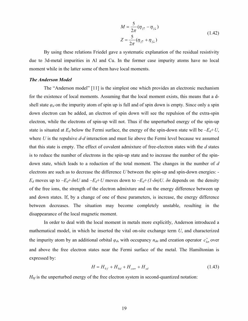
1.3 Photoelectron spectroscopy

Regarded today as a powerful surface spectroscopic technique, the photoelectron

spectroscopy (PES) strikes its roots over more than a century ago. In 1887 W. Hallwachs and H.

Hertz discovered the external photoelectric effect [35, 36] and in the following years refined

experiments by J. J. Thomson led to the discovery of the electron, thus elucidating the nature of

photo–emitted particles [37]. In 1905 A. Einstein postulated the quantum hypothesis for

electromagnetic radiation and explained the systematic involved in experimental results [38]. By

the early sixties C.N. Berglund and W. E. Spiecer extended the theoretical approach and

presented the first model of photoemission [39]. In the same period a group conducted by

K.Siegbahn in Sweden reported substantially improvements on the energy resolution and

sensitivity of so–called β–spectrometers. They used X–rays (hυ ≈ 1500 eV) and managed to

improve the determination of electron binding energies in atoms. Chemical shifts of about 1 eV

27

became detectable [40–42]. The new technique was accordingly named Electron Spectroscopy

for Chemical Analysis (ESCA). The seventies marked the full recognition of technique’s

potential as a valuable tool for the surface analysis. Accurate data on the mean free path of the

slow electrons were obtained and ultra–high vacuum (UHV) instruments became commercially

available. More on the historical development of the photoelectron spectroscopy can be found in

[43].

1.3.1. Physical principles of the technique

A PES experiment is schematically presented in Fig. 1.10. Incident photons are absorbed

in a sample and their energy may be transferred to the electrons. If the energy of photons is high

enough the sample may be excited above the ionization threshold which is accomplished by

photoemission of electrons. Their kinetic energy is measured and the initial state energy of the

electron before excitation can be traced back. Depending on the energy of incident radiation, the

experimental techniques are labeled as: Ultra–Violet Photoelectron Spectroscopy or UPS (hυ <

100 eV), Soft X–ray Photoelectron Spectroscopy or SXPS (100 eV < hυ < 1000 eV) and X–ray

Photoelectron Spectroscopy or XPS (hυ > 1000 eV).

Fig. 1.10. Schematic representation of a PES experiment

In practical XPS, the most used incident X–rays are Al Kα (1486.6 eV) and Mg Kα

(1253.6 eV). The photons have limited penetrating power in a solid on the order of 1–10

micrometers. However the escape depth of the emitted electrons is limited to some 50 ˚A. This

characteristic makes XPS to an attractive surface science tool.

For a free atom or molecule, the energy conservation before and after photoemission is

given by:

finkinin EEhE +=+ υ (1.65)

28

where inE and finE are the total initial and final energies of the atom or molecule before and after

photoemission, respectively, hυ is the photon energy and kinE is the photoelectron kinetic

energy. The binding energy ( bE ) for a given electron is defined as the energy necessary to

remove the electron to infinity with zero kinetic energy. Therefore, one can write:

bkin EEh +=υ (1.66)

In eq. (1.66) the vacuum level is considered as reference level since it corresponds to a

free atom (molecule). For the case of solids, the spectrometer and the solid are electrically

connected in order to keep the system at a common potential during photoemission. Being

connected, the Fermi levels of the spectrometer and solid become the same, as shown in Fig.

1.11 for a metal. Therefore, the kinetic energy of the photoelectron leaving the solid surface

( kinE ) will be modified by the field ( sΦ−Φ ) in such a way that in spectrometer one measures

a photoelectron kinetic energy:

)('skinkin EE Φ−Φ−= (1.67)

where Φ and sΦ [44] are the work functions of the solid and spectrometer, respectively.

Fig. 1.11. The energy levels diagram for a solid electrically connected to a spectrometer

The binding energy for the metallic solid relative to the Fermi level is then given by:

skinb EhE Φ−−= 'ν (1.68)

29

In case of semiconducting and insulating samples, the assigning of the zero binding

energy may be even more complicated and the calibration of zero binding energy is performed

with reference to some known line of an element in the sample with known valence state.

The XPS spectrum illustrates the number of electrons (recorded with the detector) versus

their kinetic energy (measured by using the electron analyzer). For practical purposes it is

generally preferred to use the binding energy as abscissa [45]. This is convenient since the

kinetic energy depends on the energy of the incident radiation and the binding energies are alone

material specific.

1.3.2 Theory of photoelectron spectroscopy

A rigorous theoretical description of the photoelectron spectroscopy implies a full

quantum–mechanical approach. In this section important aspects underlying XPS are sketched

focusing on the main approximations and models.

Let us consider a system containing N electrons which is described by the wave function

)(NinΨ and the energy )(NEin . Absorption of a photon with the energy hυ causes the

excitation into a final state described by )(NkfinΨ and )(NE k

fin [46]:

statefinalkfin

kfin

hstateinitial

inin NENNEN__

)();()();( Ψ⎯→⎯Ψ υ (1.69)

where k labels the electron orbital from which the photoelectron has been removed. The

transition probability (which dictates the photocurrent intensity) obeys the Fermi’s golden rule

[47]:

υδπ hNENENNw inkfin

kfinin −−ΨΗΨ= )()(()()(2 2

h (1.70)

where the δ function ensures the energy conservation during transition and H is the interaction

operator. The eq. (1.70) is satisfied when the perturbation H applied to the system is small. The

interaction operator can be written as:

( ) AAcm

eepAApcm

e

ee2

2

22+−+=Η ϕ (1.71)

Here e and em denote the electron charge and mass, c is the light speed, A and ϕ are the

vector potential operator and respectively the scalar potential of the exciting electromagnetic

field and p is the momentum operator of the electron. A simplified form of the interaction

Hamiltonian can be obtained by assuming that the two–phonon processes can be neglected (the

30

term AA ), that the electromagnetic field can be described in the dipole approximation and

choosing 0=ϕ [48]:

pAcm

eHe

0= (1.72)

where 0A is the constant amplitude of electromagnetic wave. The dipole approximation is valid

if the radiation wave–length is much larger than atomic distances, which is correct for the visible

and ultraviolet regions of the electromagnetic spectrum. Mathematically the vector potential

operator can be then written as )(0),( tkreAtrA ω−= . The approximation interaction

Hamiltonian for the structure of final state is more subtle [48, 49].

For high energy spectroscopy it can be assumed that the outgoing electron is emitted so

fast that it is sufficiently weak coupled to the (N − 1) electron ion left behind. This is the so–

called sudden–approximation which is actually valid in the keV region of energies. For lower

energy regions its applicability has certain restrictions [50, 51]. The final state can be split up in

two configurations: ronphotoelect

kkin

kionstatefinal

kfin

kfin

hstateinitial

inin ENENNEN );1()();1()();(___

ξυ +−Ψ⎯→⎯Ψ (1.73)

where )1(kξ is the wave function of the photoelectron.

The energy conservation during photoemission simply yields:

Φ++−=+ kkin

kfinin ENEhNE )1()( υ (1.74)

Here Φ is the work function. According to eq. (1.68) the binding energy with respect to the

Fermi level may be defined as:

)()1( NENEE inkfin

kb −−= (1.75)

Koopmans assumed that the above binding energy difference can be calculated from Hartree–

Fock wave functions for the initial as well as for the final state [52]. The binding energy is then

given by the negative one–electron energy of the orbital from which the electron has been

expelled by the photoemission process:

kkbE ε−= (1.76)

This approach assumes that the remaining orbitals are the same in the final state as they were in

the initial state (frozen–orbital approximation) and leaves out the fact that after the ejection of an

electron the orbitals will readjust to the new situation in order to minimize the total energy. This

31

is the intra–atomic relaxation. In fact the relaxation also has an extra-atomic part connected with

the charge flow from the crystal to the ion where the hole was created. Therefore the binding

energy is more accurately written as:

relaxkkbE δεε −−= (1.77)

where relaxδε is a positive relaxation correction. An even more rigorous analysis must take into

account relativistic and correlation effects which are neglected in the Hartree–Fock scheme.

Usually both increase the electron binding energy.

1.3.3 Photoelectron spectroscopy models

Three–step model

In frame of this model the complicated photoelectron processes broken up into three independent

events [39]:

(I) absorption of a photon and photo–excitation of an electron as described above;

(II) transport of the electron to the surface;

Some of the photoelectrons reach the surface of the solid after suffering scattering

processes, the dominant scattering mechanism being the electron–electron interaction. For low

energies electron–phonon interaction dominates [53]. One of the most important parameter

which describes these processes is the inelastic mean free pathλ . It is defined as the mean

distance between two successive inelastic impacts of the electron on its way through the crystal.

Assuming that the mean free path λ is isotropic, several calculations were performed and an

universal dependence curve of the mean free path was drawn [53–55]. More recent results based

on Bethe’s equation [56] came up with [57]:

)ln()( 2 EE

EEplas γβ

λ = (1.78)

where λ will be deduced in (Å), E is the electron energy given in (eV ), β and γ are

parameters. Eplas is the plasmon energy of the free electron gas in (eV) and it can be calculated

with MNE vplas /8.28 ρ where vN is the number of valence electrons per molecule, ρ is

the density and M is the molecular mass. An extended approach based on a modified Bethe

equation delivers even better results [58–63]. For practical purposes the reduced

32

formula pE∝λ , where p ranges from 0.6 to 0.8, can be used since it delivers reasonable results

of the mean free path for electron energies in 100–1000 eV range [64].

(III) escape of the electron into vacuum;

The escaping electrons are those for which the component of the kinetic energy normal to

the surface is enough to overcome the surface potential barrier. The other electrons are totally

reflected back.

One–step model

Apart from its didactic simplicity, the three–step model fails to offer a practical computational

tool for the simulation of photoelectron lines. State of the art is the employing of one–step

theoretical approaches in which the whole photoelectron process is regarded as a single one. The

first of this kind was a compact and mathematically elegant solution to the previous three-step

model [65] but was followed by fully dynamical [66] and relativistic one–step theories [48].

When specific crystal potentials are given as input data one–step models deliver theoretical

simulations of the XPS spectra [67].

1.3.4 Spectral Characteristics

The first step which is taken generally in the sample characterization is the recording of a

wide scan. This so called survey spectrum allows identifying the chemical components in the

sample and to define acquisition windows. The lines which are of interest are recorded

afterwards with a high resolution.

The XPS spectra can be divided into: primary spectrum which is given by the electrons

which leave the solid without inelastic scattering processes, and secondary spectrum arising from

photo-electrons which have already lost a percentage of their kinetic energy trough inelastic

scattering processes on their way to the surface.

1.3.4.1 Core level lines

Photoemission produces a final state that is lacking one electron with respect to the initial

state. Therefore PES (photoemission spectroscopy) always measures final-state energies which

can be related to initial-state energies only after some theoretical considerations, as it was

mentioned in the last paragraph. The XPS lines associated with the core levels may have variable

intensities and widths, which, except for the s levels, are doublets. Photoelectrons, which

originate from core-levels, give rise to the most intensive lines in the XPS spectra. The position

of the core level lines is like a fingerprint for each element and thus the chemical identification

33

of the components in the investigated specimen can be easily performed. Generally two or more

elements will be detected on the surface. The relative intensities of their lines are governed by:

occupancy of the sub–shell, stoichiometry, and atomic cross-sectionσ . The values of σ can be

derived from X-ray mass absorption coefficients or can be directly calculated [68, 69]. Since the

occupancy of the atomic sub-shells is known, XPS can be used as a non-destructive chemical

analysis tool.

Core-level lines shape and width

The width of the peak is defined as the full width at half maximum intensity (FWHM).

This is a sum of three distinct contributions [70]: the natural inherent width of the core-level nγ ,

the width of the photon source pγ and the analyzer resolution aγ . Thus the overall FWHM will

be given by:

222apn γγγγ ++= (1.79)

The first contribution is dictated via the uncertainty principle h≥ΔΔ tE by the core-hole life

timeτ .

τγ h

n = (1.80)

where h is the Plank constant. The lifetimes depend on the relaxation processes which follow

the photoemission. The narrowest core-levels have lifetimes in the range 10−14 −10−15 s whilst the

broader have lifetimes close or slightly less than 10−15s.

A range of physically possible line profiles in core-level XPS is possible, and simple

Gaussian or Lorentzian functions are very rarely adequate. In the case of metal samples it has

been shown that asymmetric profiles should be expected on theoretical grounds [71], however,

recorded spectra exhibit deviations from idealized profiles due to a range of instrumental and

physical effects:

• the response function of the electron analyzer;

• the profile of the X-ray line-shape;

• intrinsic life-time broadening of the core level hole state;

• photon broadening;

• differential surface charging of the sample.

In addition to the instrumental considerations the shape of a synthetic peak is also influenced by

the choice of background algorithm used to remove the so-called extrinsic electrons from the

34

data. The intrinsic part of the XPS peak due to the core-level life time is described by a Lorentz

function: 1

2

241)(−

⎟⎟⎠

⎞⎜⎜⎝

⎛+=

nLf

γεε (1.81)

where 0EE −=ε is the difference relative to the maximum of the curve. The overall line

shape of core lines are obtained by convoluting the above two functions in a resulting so-called

Voigt profile:

∫+∞

∞−

−=⊗= ')'()'( εεεε dfffff GLGLL (1.82)

Doniach and Sunjic [71] have shown that in metals the core level lines have a characteristic

asymmetrical shape:

( )( )

( )[ ] 21

22 2/

2arctan12

cos1),( α

γε

γεααπ

ααε −

+

⎥⎦

⎤⎢⎣

⎡⎟⎟⎠

⎞⎜⎜⎝

⎛−+

−Γ=

n

nDSf (1.83)

where Γ is the gamma function, dtetz tz −+∞

∞−

−∫=Γ 1)( , and α is an asymmetry parameter.

The values of α can range between 0.1 and about 0.25 [72]. For the case of non-conducting

samples the asymmetry factor is equal to zero and )()0,( εε LDS ff = . The asymmetry of the

intrinsic XPS lines of conducting samples can be explained by taking into account the nonzero

density of states at the Fermi level.

Spin-orbit coupling

In terms of a j − j coupling scheme between angular and spin moments in an atom, for

each orbital with nonzero angular quantum number l (l > 0), two energy levels are possible for

electrons: the first with total quantum number j = l + s and the second with j = l − s (where s is

the spin quantum number).

This spin–orbit splitting is present in XPS spectra; two peaks being observable, each for

one j value. Taking into account that for a given j value there are (2j + 1) allowed states for

electrons and that s = 1/2, the ratio of relative intensities can be easily calculated:

35

11212

1212

+=

−⎟⎠⎞

⎜⎝⎛ +

+⎟⎠⎞

⎜⎝⎛ −

=+=

−=

ll

l

l

II

slj

slj (1.84)

High–resolution core–level spectroscopy studies show small deviations from this

branching–ratio due to different cross sections for the j = l + s and j = l − s lines and photo–

diffraction effects.

Chemical shifts

In the investigation of the molecules and solids, one is not interested in the absolute binding

energy of a particular core level, but in the change in binding energy between two different

chemical forms of the same atom. This difference is the so-called chemical shift [45]. The

chemical shift between a metal and its oxide can be used to monitor the surface cleanliness.

Multiplet splitting

In any atomic system with unpaired valence electrons, the exchange interaction affects

spin-up and spin-down core electrons differently. Since exchange acts only between electrons

with the same spin [73], core electrons with spins parallel to those of the unpaired valence

electrons will experience a valence-electron exchange potential, whereas core electrons with

spins antiparallel will not. Exchange interactions within or between closed shells balance exactly,

as the numbers of electrons with same spin are equal. This interaction between core and unpaired

valence electrons is responsible for core-polarization contributions to magnetic hyperfine

structure [74]. The spectral splitting of the 3s core-level x-ray photoemission spectra (XPS) in

transition metals and their compounds originates from the exchange coupling between the 3s

hole and the 3d electrons and was experimentally observed about three decades ago [75, 76]. The

magnitude of the 3s spectral splitting according to the van Vleck theorem [77] is determined by:

( )dsGlSEex 3,3

1212 2

++

=Δ (1.85)

where S is the total spin of the ground state of the 3d electrons, l is the orbital quantum number

( l =2) and ( )dsG 3,32 is the Slater exchange integral. The intensity ratio for the two peaks is

proportional in this model to the ratio of the angular momentum multiplicity:

SS

S

S

II

S

S 1

1212

1212

2/1

2/1 +=

+⎟⎠⎞

⎜⎝⎛ −

+⎟⎠⎞

⎜⎝⎛ +

=−

+ (1.86)

36

The value of the multiplet splitting gives information about the total spin of 3d band [45]. The

multiplet splitting of 2p3/2 line was observed in compounds with strong localized moments [78].

Satellites line

In the photoemission process the photon kicks out one electron so quickly that the

remaining electrons do not have time to readjust. Thus the (N − 1) electron system is left in a

non–relaxed state finΨ . This excited state has a certain overlap with the stationary states nΨ

and according to the sudden approximation we obtain the probabilities finn ΨΨ to end up in

nΨ states [79]. This means that the XPS spectrum consists from the main line (corresponding to

the lowest excited state) and a number of extra lines (so–called satellites) representing the higher

excited states after photoemission.

In principle, there are two sources of satellites: an extrinsic part due to the extra–atomic

events and an intrinsic part due to the intra–atomic relaxations.

The reorganization of electronic structure after the creation of a core hole could also lead

to an excess of energy which is not available to the primarily excited photoelectron. Thus two–

electron processes can occur in case of conducting samples. The corresponding structures in the

spectra are denoted as shake satellites. The hole appears to increase the nuclear charge and this

perturbation is the cause of valence electrons reorganization. It may involve the excitation of one

of them to a higher energy level. If an electron is excited to a higher bounded state then the

corresponding satellite is called shake–up satellite. If the excitation occurs into free continuum

states, leaving a double ionized atom with holes both in the core level and valence shell, the

effect is denoted as a shake-off satellite from [80]). Discrete shake-off satellites are rarely

discerned in the solid [70].

1.3.4.2 Valence band

Whereas the core levels are usually reacted by well-resolved sharp XPS peaks, the

valence band spectra are characterized by a band structure (many closely spaced levels) [70].

The valence electrons involved in the delocalized or bonding orbitals have low binding energies

(< 20 eV). Because of the lower cross-sections of the valence photoelectrons as compared to the

core photoelectrons, the valence band spectra intensity will appear much lower than for the core

level spectra.

37

The valence band spectrum resembles the one–electron density of states curve, but due to

certain facts they are not identical: the spectrum represents the DOS distribution in an excited

state, several screenings of the created hole (many–body effects), emission of electrons with

different quantum numbers (i.e. different sub-shell cross–sections) or from different atomic

species (i.e. different atomic cross–sections) as well as the instrumental broadening being

responsible for further modifications.

One way to interpret the XPS VB spectra is the comparison with theoretical calculations

of the densities of states (DOS). The recorded spectra can be simulated when such calculations

are available and thus the contribution of each sub–shell can be described. Another alternative is

to employ different excitations energies. The relative intensities of the various valence electrons

peaks can drastically change when varying the energy of the used radiation because the relative

photo–ionization cross sections change versus the incident photon energy. For example, by

comparing the UPS and XPS valence band spectra of a MxO oxide, one can get information

about the partial contributions of the metal and oxygen states in the valence band. Another

modern alternative is the interpretation of XPS VB in connection with other spectroscopic

techniques like X–ray emission spectroscopy. In such joint VB studies certain features of the

spectra can be directly assigned to the elemental components.

1.3.4.3 Secondary spectra (background)

During their transport to the surface, some photoelectrons lose part of their energy through

inelastic scattering processes and end up at a lower energy in the spectrum, giving rise to a

background. For quantitative analysis of the XPS spectra, the true peaks areas and their shapes

need to be determined. Therefore, usually background corrections are applied. Shirley was the

first to deal with this problem and he proposed a practical model [81]. However its results are in

most of the cases unsatisfactory. In the Tougaard algorithms [82-85] the measured spectrum

( )Ej is considered to consist of a primary photoelectron spectrum ( )EF and background, as

given:

( ) ( ) ( ) ( )∫∞

′−+=E

EdEjEEEKEEFEj '',)(λ (1.87)

where )',( EEEK − describes the probability that an electron with the energy E losses the

energy )'( EE − during a mean free path travel. The second term in eq. (1.87) gives the

38

background correction. A universal loss function ),()( TEKEλ which should describe all pure

materials was proposed:

( ) ( ) ( )( )[ ]22

,TC

TBTEKE+

=λ (1.88)

where B and C are two constants. By comparison with experimental data, it was shown that the

background correction for pure Ag, Au and Cu can be described using the following values: B =

2866 eV2 and C = 1643 eV2. In case of alloys this universal loss function delivers a general good

fit with experiment. An accurate background can be obtained only from EELS (Electron Energy

Loss Spectroscopy) experiments. In an EELS experiment electrons with kinetic energy E0 are

sent on the sample. A certain part of them will be reflected but the rest enter the surface and

interact with the solid. Due to scattering processes the electrons lose energy LE and leave the

solid with the kinetic energy LS EEE −= 0 . The outgoing electrons are recorded energy

resolved. In other words such an experiment simulates the kinetic energy loss of the XPS

electrons [86].

1.3.4.4 Auger process

After photo–emission the core hole will be filled with an electron decaying from a higher

occupied level. This recovery of the atom from a higher energy state may be accomplished by

the photo–ejection of another electron. This two–electron process takes place on a 10−14 seconds

time scale and is known as an Auger process. Fig. 1.12 presents a schematic energy level

diagram of a solid, in which the energy is measured downwards from an assumed zero of energy

at the Fermi level.

Fig. 1.12. Schematic diagram of the process of Auger emission in a solid (after [87])

39

In this example the K level is being ionized by an incident electron, whose energy pE must be

greater than the binding energy KE of an electron in the K shell. Following creation of a hole

in the level K , the atom relaxes by filling the hole via a transition from an outer level, in this

example from the as 1L level. As a result of that transition the energy difference ( )1LK EE − can

be used by the atom in either of two ways. It can appear as a characteristic X-ray photon of that

energy or it can be given to another electron either in the same level or in a more shallow level,

whereupon the second electron is ejected. This first process is that of X-ray fluorescence, the

second that of Auger emission. Both cannot take place from the same initial core hole, so that

they complete. The Auger transition depicted in Fig.1.12, would be named in the conventionally

used jj − coupling 3,21LKL . The electrons taking part in the Auger process might also

originate in the valence band of the solid, in which case the convention writes the transitions as,

for example, VKL 3,2 if one electron comes from the valence band and, for example, KVV if

both do. The energy of the ejected Auger electron is given by: *

3,213,21 LLKLKL EEEE −−=

where iE is the binding energies of the i -th atomic energy level. *

3,2LE is starred because is the

binding energy of the 3,2L level in the presence of a hole in level 1L , and is therefore different

from 3,2LE .

40

Chapter 2 Preparation and Characterization techniques

2.1 Sample preparation

Polycrystalline samples were prepared by arc melting technique in a cold copper crucible

under an argon atmosphere. High purity starting materials (>99.99%) were weighted in exact

stoichiometric proportions and melted together. To ensure a good homogeneity of the samples,

the compounds were melted several times in the same atmosphere. This preparation method

preserves the phase from high temperatures. The weight loss of the final samples was found to be

less than 1%. The homogeneity of the samples was checked by conventional X-ray diffraction

technique. XRD measurements were performed on polished surfaces, due to the hardness of the

samples. The quality of the samples, in terms of contamination, was also investigated by

monitoring the oxygen and carbon 1s core levels by means of X-ray photoelectron spectroscopy.

2.2 Structure analysis

The crystallographic structure of all the samples was checked at room temperature using

X-ray powder diffraction data. The interaction of X-rays with crystalline sample creates

secondary diffracted beams of X-rays related to interplanar spacing in the crystalline powder

according to the Bragg’s Law:

θλ sin2dn = (2.1)

where n is an integer, λ is the wavelength of the incident X-ray beam, d is the interplanar spacing

and θ is the diffraction angle. A typical powder diffraction pattern is collected in the form of

scattered intensity as a numerical function of Bragg angle. The structure of every powder

diffraction is determined by the unit cell dimensions and the atomic structure (unit cell content

and special distribution of atoms in the unit cell) and can be thus be used to determine the

crystalline structure of the samples. The individual Bragg peaks are located on the pattern and

both their position and intensity are determined. The peak positions are used to establish the unit

cell symmetry, parameters and content, while the peak intensities are used to determine space

group symmetry and coordinates of atoms.

The structure investigation of the compounds was performed by conventional X-ray

powder diffraction with Cu Kα radiation, using a Bruker AXS D8 Advance powder

diffractometer. This instrument is based around a two circle goniometer, enclosed in a radiation

41

safety enclosure. The working principle of a Bragg-Brentano reflection goniometer is presented

in Fig. 2.1.

The X-ray source is a 2.2 kW Cu anode situated in a long fine focus ceramic X-ray tube.

The running conditions for the X-Ray tube are 40 kV and 40 mA. The sample stage is mounted

on the goniometer for precision angle measurement. The two circle goniometer has independent

stepper motors and optical encoders for the Theta and 2Theta circles with the following

specifications: maximum measurement circle diameter of 250 mm, minimum measurement circle

diameter of 100 mm, smallest angular step size of 0.0001o, maximum rotational speed of

1500o/min, angular range (Theta) from -5o to 40o, angular range (2Theta) from -10o to 60o. The

detector is a NaI dynamic scintillation detector with 2x106 s-1 maximum count rate.

Fig. 2.1. Schematic diagram of a Bragg-Brentano Diffractometer

A computer controlled absorber is mounted directly in front of the detector and is used to

attenuate the beam by about two orders of magnitude. To change the angular resolution several

slits (0.05 to 2 mm) are available to be placed in front of the detector, as are a set of Soller slits to

allow acquisition for small samples. Attenuators made of Cu and Ni are also available and can be

manually placed in the beam, by inserting them into the slit holders in front of the detector. The

detector electronics are capable of a 3x107 s-1count rate. In addition, the D8 Advance

diffractometer can be equipped with a chamber for variable temperature or low pressure

experiments. The software used enables the user to acquire and analyze data. For qualitative

analysis the Rietveld method [88] was employed.

42

2.3 Magnetic measurements

The macroscopically magnetic properties (magnetic order, transition temperatures,

magnetic moments, the contribution of each element to the total magnetization of the compound)

were investigated by static and dynamic magnetic measurements in fields up to 10 T and

temperature range of 4.2 – 1200K. A vibrating sample magnetometer (VSM) was used to

measure the field and temperature dependence of the magnetization in order to determine the

transition temperature and the value of the spontaneous magnetization at 0 K by extrapolation. A

SQUID magnetometer was used to measure the magnetic susceptibility in field cooled (FC) and

zero field cooled (ZFC). In the paramagnetic range (above the transition temperature) the

variation of the magnetic susceptibility with the temperature was obtained using a Weiss balance

and magnetic fields up to 1 T. The magnetic characterization of the investigated systems was

realized by correlating the data from both ordered and paramagnetic states, which allowed the

calculation of magnetic moments and the contribution of each element to the total magnetization

of the compound.

2.3.1 Vibrating sample magnetometer

The Vibrating Sample Magnetometer (VSM) represents by far the most commonly used

type of magnetometer. Since its invention some forty years ago, it has become the workhorse in

both laboratory and production environments for measuring the basic magnetic properties of

materials as a function of magnetic field and temperature.

The VSM, shown schematically in Fig. 2.2, employs an electromagnet which provides

the magnetizing field, a vibrator mechanism to vibrate the sample in the magnetic field, and

detection coils which generate the signal voltage due to the changing flux emanating from the

vibrating sample. The output measurement displays the magnetic moment M as a function of the

field H.

VSM operates by first placing the sample to be studied in a constant magnetic field,

which will magnetize the sample. The stronger the constant field, the larger the magnetization

will be. The sample is located at the end of a rigid holder attached to the vibration exciter and

can oscillate in the vertical direction, perpendicular to the magnetic field. The sample rod can be

rotated to achieve the desired orientation of the sample to the constant magnetic field. As the

sample is moved up and down, it produces an alternating current in the detection coils at the

same frequency as the vibration of the sample, according to Faraday's Law of Induction. The

induction current which is proportional to the magnetization of the sample is then amplified by

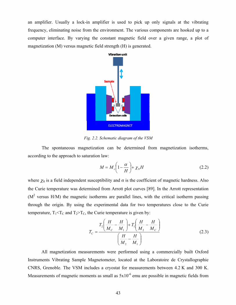
43

an amplifier. Usually a lock-in amplifier is used to pick up only signals at the vibrating

frequency, eliminating noise from the environment. The various components are hooked up to a

computer interface. By varying the constant magnetic field over a given range, a plot of

magnetization (M) versus magnetic field strength (H) is generated.

Fig. 2.2. Schematic diagram of the VSM

The spontaneous magnetization can be determined from magnetization isotherms,

according to the approach to saturation law:

HH

MM s 01 χα+⎟

⎠⎞

⎜⎝⎛ −= (2.2)

where χ0 is a field independent susceptibility and α is the coefficient of magnetic hardness. Also

the Curie temperature was determined from Arrott plot curves [89]. In the Arrott representation

(M2 versus H/M) the magnetic isotherms are parallel lines, with the critical isotherm passing

through the origin. By using the experimental data for two temperatures close to the Curie

temperature, T1<TC and T2>TC, the Curie temperature is given by:

⎟⎟⎠

⎞⎜⎜⎝

⎛−

⎟⎟⎠

⎞⎜⎜⎝

⎛−+⎟⎟

⎠

⎞⎜⎜⎝

⎛−

=

12

21

12

MH

MH

MH

MHT

MH

MHT

T CCC (2.3)

All magnetization measurements were performed using a commercially built Oxford

Instruments Vibrating Sample Magnetometer, located at the Laboratoire de Crystallographie

CNRS, Grenoble. The VSM includes a cryostat for measurements between 4.2 K and 300 K.

Measurements of magnetic moments as small as 5x10-6 emu are possible in magnetic fields from

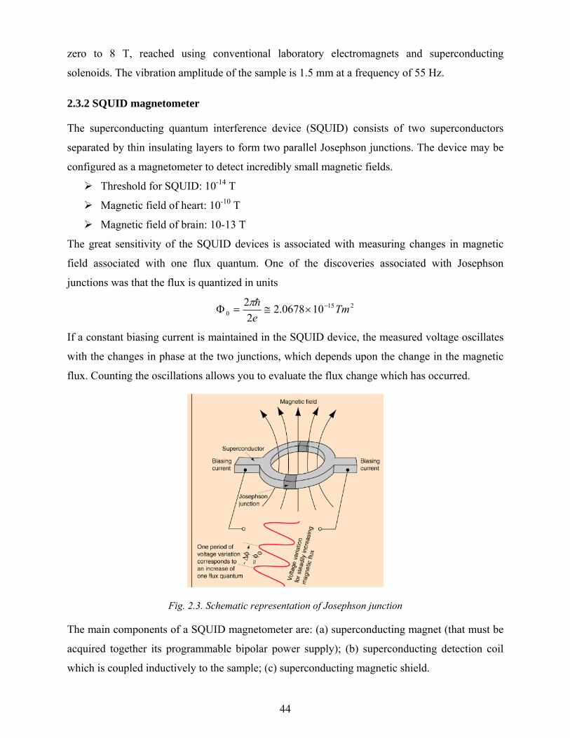
44

zero to 8 T, reached using conventional laboratory electromagnets and superconducting

solenoids. The vibration amplitude of the sample is 1.5 mm at a frequency of 55 Hz.

2.3.2 SQUID magnetometer

The superconducting quantum interference device (SQUID) consists of two superconductors

separated by thin insulating layers to form two parallel Josephson junctions. The device may be

configured as a magnetometer to detect incredibly small magnetic fields.

Threshold for SQUID: 10-14 T

Magnetic field of heart: 10-10 T

Magnetic field of brain: 10-13 T

The great sensitivity of the SQUID devices is associated with measuring changes in magnetic

field associated with one flux quantum. One of the discoveries associated with Josephson

junctions was that the flux is quantized in units

2150 100678.2

22 Tm

e−×≅=Φ

hπ

If a constant biasing current is maintained in the SQUID device, the measured voltage oscillates

with the changes in phase at the two junctions, which depends upon the change in the magnetic

flux. Counting the oscillations allows you to evaluate the flux change which has occurred.

Fig. 2.3. Schematic representation of Josephson junction

The main components of a SQUID magnetometer are: (a) superconducting magnet (that must be

acquired together its programmable bipolar power supply); (b) superconducting detection coil

which is coupled inductively to the sample; (c) superconducting magnetic shield.

45

Fig. 2.4.a) Schematic of SQUID magnetometer; b) calibrated output from SQUID electronics

A superconducting magnet is a solenoid made of superconducting wire. This solenoid must be

kept at liquid helium temperature. The uniform magnetic field is produced along the axial

cylindrical bore of the coil. To operate a superconducting magnet requires an appropriate

programmable bipolar power supply.

Superconducting detection coil is a single piece of superconducting wire configured as a second-

order gradiometer. This pick-up coil system is placed in the uniform magnetic field region of the

solenoid superconducting magnet.

Superconducting magnetic shield is used to shield the SQUID sensor from the fluctuations of the

ambient magnetic field of the place where the magnetometer is located and from the large

magnetic field produced by the superconducting magnet.

2.3.3 Weiss balance

The Weiss horizontal translation balance is a very sensitive instrument designed

especially for investigating weak magnetic substances (diamagnets, antiferromagnets, spin-

glasses) and for very small samples (about 10 mg), since it can measure magnetic susceptibilities

as small as 10-7. The detection of magnetic moments is done by measuring the force on a sample

in an inhomogeneous magnetic field generated by an electromagnet. The inhomogeneity of the

magnetic field between the poles of the electromagnet is determined by the shape of the caps.

The force on a magnetic sample in the field gradient is given by:

dxdHHmF χμ0= (2.4)

46

Electromagnet

SampleQuartz tube

Heating element

Compensation frame

Compensation coil

Mirror

Diode laser

Graded scale

Balance rod

Amortizationsystem

Electromagnet

SampleQuartz tube

Heating element

Compensation frame

Compensation coil

Mirror

Diode laser

Graded scale

Balance rod

Amortizationsystem

Fig. 2.5. Schematic diagram of a Weiss magnetic balance

As soon as the gradient dH/dx is known, it is easy to evaluate the magnetic susceptibility

χ of a sample from the observed force.

The main components of the Weiss magnetic balance located in our laboratory are

sketched in Fig. 2.5. The sample is housed in a quartz cup at the end of a horizontal quartz rod,

connected to the balance beam, and is situated inside a quartz tube which is, between the pole

caps, surrounded with a heating element in order to change the temperature. In order to guarantee

proper force detection, the sample holder has to hang free from the walls of the surrounding tube.

The balance rod is hanged in a horizontal position by two inextensible wires that allow free

movement along the horizontal x-direction. The temperature is measured with thermocouples

situated inside the quartz tube in the proximity of the sample. The current through the heating

elements is controlled by a computer, allowing the programming of measurements at a user

defined equidistant series of temperatures. The electromagnet used can generate magnetic fields

up to 1.5 T. Our pole caps are cut so that on the symmetry axis of the magnet (x-direction) the

product HdH/dx is constant over a considerable range in which the sample can move. The force

generated by this gradient field will act along the x direction, producing a deviation of the laser

beam spot on the graded scale in the optical system situated at the end of the balance rod. If the

sample is at a position where the field gradient is known, the magnetic susceptibility can be

evaluated from this deviation. A compensating coil system consisting of a rectangular frame

fixed on the balance rod and two Helmholtz concentric coils is used to determine the force

exerted on the sample. One side of the frame is situated outside the coils, while the opposite one

is located in the centre of the Helmholtz coils perpendicular to the magnetic filed. An electrical

current I applied through the frame will generate an axial compensatory force:

47

lBIF cc = (2.5)

where B is the magnetic induction of the field generated by the Helmholtz coils and l is the

length of the frame. This force is used to compensate the force given by Eq. (2.4).

dxdHHmlBIc χμ0= (2.6)

The zero deviation position is determined for zero magnetic fields (H=0, B=0) and no current

through the frame (Ic=0). All these parameters are computer controlled. Considering that the

magnetic induction B of is proportional to the current through the Helmholtz coils (B=αIH):

dxdHHmIlIIlI diaHcHc χμαα 0)( =+ (2.7)

where the second term is for the diamagnetic contribution of the balance rod. The measurement

consists in compensating the effect of the applied magnetic field H on the sample by varying the

compensatory currents in the Helmholtz coils and in the frame.

After performing a calibration by measuring the well known susceptibility of a small quantity of

nickel of purity 99.999%, the magnetic susceptibility of an unknown sample is:

mIIII

km

IIIIIIII

m diaH

diac

iHc

diaH

diac

iHc

diaH

diac

NiH

Nic

NiNi

)()()(

+=

++

= χχ (2.8)

The effective magnetic moments for ferromagnetic and antiferromagnetic materials can be

determined from the temperature dependence of the reciprocal susceptibility above the transition

temperature, where the magnetic susceptibility obeys the Curie-Weiss law. This assumption is

valid also for ferrimagnetic materials, for which the high temperature asymptote to the Néel

hyperbolic law has a Curie-Weiss behavior. The molar Curie constant C is obtained from the

slope of the temperature dependence of the reciprocal susceptibility at high temperatures, by

linear fitting, and the magnetic moment is calculated as:

Ceff 84.2≅μ (2.9)

If more than one type of atoms contributes to the magnetic susceptibility of the material, the

molar Curie constant is given by:

∑=i

iCC (2.10)

2.4 X- ray photoelectron spectroscopy

The electronic structure of the materials was investigated by means of X-ray

photoelectron spectroscopy, which was presented in the previous chapter. The XPS experiments

48

were performed using a commercially available spectrometer PHI Model 5600 Multi-Technique

System produced by the Perkin Elmer Corporation, located at the Osnabrück University. The

PHI spectrometer is built up from: a control computer, electronic control units, a ”quick-entry”

system and a main and preparation chamber. The bulk samples were crushed in situ in the

preparation chamber in high–vacuum conditions (usually around 7x10−8 torr), in order to prevent

surface contamination, and then transferred to the main chamber where the measurements were

performed. A quick–entry system is also available allowing a rapid, convenient, and direct

introduction of samples into the main chamber.

The main components of the spectrometer, which is situated in the main chamber, are

sketched in Fig. 2.6.

Fig. 2.6. Schematic diagram of the PHI 5600 spectrometer

The spectrometer is equipped with Al anode for measurements with monochromatic radiation

and a dual Al/Mg anode positioned in an angle of 54.7o to the analyzer. The characteristic energy

and half–widths for the unmonochromatized radiations are: 1486.6 eV and 0.85 eV for Al Kα

radiation and 1253.6 eV and 0.7 eV for Mg Kα radiation. The Al Kα characteristic radiation is

filtered through a monochromator consisting of an accurate quartz crystal. The Al anode-crystal-

sample angle is 23o, as resulted from the Bragg relation for the first order diffraction of Al Kα

radiation (λ = 8.34°A) and d = 4.255°A spacing of the (100) planes. The crystal–sample–

analyzer angle is fixed to 90o. The monochromator focuses the radiation to a spot of 0.9 mm on

the sample due to its toroidal shape, reduces the half-width to about 0.3 eV, eliminates the

49

satellites of characteristic Al Kα radiations and improves the signal to background ratio. All the

XPS spectra were measured using monochromatic radiation from an Al anode with 12 kV

accelerating potential and powered with 250 W. The energy of the photoemitted electrons is

filtered using an 11 inches hemispherical condenser. The photoelectrons are focused with an

electronic lens system and then enter the analyzer through an entrance slit which can be set to 4,

2, 0.5 or 0.15 mm. During all XPS measurements the ”constant analyzer transmission” (CAT)

mode was used, so that only the electrons with the energy Ep±ΔE (where Ep is the ”pass-energy”

and ΔE is the absolute energy resolution) passed through the analyzer. The relative resolution of

the analyzer is given approximately by [90]:

00

63.0Rw

EE≈

Δ (2.11)

where E0 is the kinetic energy of the entering electrons and R0 is the median radius of the

hemispherical analyzer. For a R0 = 11 inches analyzer and a w = 2 mm entrance slit, the absolute

resolution of the analyzer is about 0.45% of the pass energy, considering that in the CAT mode

E0 corresponds to the pass–energy. For the detection of the electrons a multi channel detector

with 16 channel plates is employed. The system also contains an ion gun with argon which can

be used to perform sputter-etching of the samples. The ions can be accelerated to 4.5 kV

maximal potential with a 3 μA available ion–current over a 10mm × 10mm scannable surface

and a 100 μm focus. However, the ion gun was not used for the present work, due to the fact that

even low accelerating potentials may induce drastic changes in surface geometry and/or

stoichiometry [87]. For insulating samples a low-energy electron gun can be used to compensate

the superficial local charges accumulated on the surface. The accelerating potential can be

chosen between 0 and 10 V at a maximal current of 25 μA. All components of the main chamber

ware kept under UHV during the experiments. There are two important reasons why ultra–high

vacuum (UHV) conditions are requested when performing XPS measurements. In order for the

photoelectrons to reach the analyzer without being scattered by gas molecules a basic vacuum in

the 10−5 torr range is required. However under such a pressure the surface of the sample is

quickly contaminated. In order to avoid surface contamination during the measurements, which

can take up to several hours, a base pressure of about 10−10 torr must be ensured. UHV conditions

are reached by employing a combination of appropriate turbo molecular, sputter and sublimation

vacuum pumps. During the recording of the XPS spectra presented in this work the base pressure

in the main chamber was maintained below 1×10−9 torr.

50

2.5 Electronic structure calculations Theoretical investigations of the electronic and magnetic properties of selected alloys and

compounds have been performed using the Munich SPR-KKR package version 3.6 [91]. The

electronic structure of the alloys and compounds in the ferromagnetic state were calculated self-

consistently by means of the spin polarized relativistic Korringa–Kohn–Rostocker (KKR)

method in the atomic sphere approximation (ASA) mode [92-94]. Several different properties

can be investigated by means of the SPRKKR package on the basis of the fully relativistic

electronic structure calculation, especially response functions and spectroscopic properties.

The calculation method is based on the KKR-Green’s function formalism that makes use

of multiple scattering theory. This implies that the information on the electronic structure of a

system is not expressed in terms of Bloch wave functions and eigenvalues but the corresponding

Green’s function. The method is based on the following Dirac-Hamiltonian for a spin-polarized

system:

( ) ( ) ( ) ( )rrrBrVmcci iiieffeff

rrrrrrrrhΨ=Ψ⎥⎦

⎤⎢⎣⎡ ⋅+++∇⋅ εσββα 2 (2.12)

where )(rir

Ψ are four-component wave functions with corresponding single particle energies iε ,

α and β are the standard 4x4 Dirac matrices, and the effective potential effV contains the

external contributions. The effective magnetic field is given by:

( ) ( ) [ ]( )rm

mnErBrB xc

exteff rr

rrrrr

∂∂

+=,

(2.13)

where Exc is the exchange and correlation energy which depends on the particle density n and

spin magnetization density m. Within the multiple-scattering formalism the electronic Green’s

function for an ordered system with many atom sites per unit cell is given by:

( ) ( ) ( )

( ) ( ) ( ) ( ) ( ) ( )[ ] qqnnqqqq

qqnnqq

rrErZErJrrErJErZ

ErZEErZErrG

′′Λ

×ΛΛ

×ΛΛ

Λ′Λ

×′Λ′

′′Λ′ΛΛ

∑

∑

−′Θ′+−′Θ′−

−′=′

δδ

τ

,,,,

,)(,,,,

rrrr

rrrr

(2.14)

where )(rr rr ′ is assumed to be within the unit cell )(nn ′ and atomic site )(qq ′ and )(Eqnnq ′′Λ′Λτ is

the scattering path operator with the combined index Λ=(κ,μ) standing for the spin-orbit and

magnetic quantum numbers κ and μ, respectively. The four-component wave functions qZΛ and

qJΛ are the properly normalized regular and irregular solutions to the single-site Dirac equation

for the atomic site q. The scattering path operator [95] transfers a wave with spin angular

51

character Λ’ coming in at site q’ into a wave outgoing from site q with character Λ taking into

account in a consistent way all possible multiple scattering events in a many-atom system. In the

case of ordered infinite systems, )(Eqq ′Λ′Λτ for one atom per unit cell is obtained from the

Brillouin-zone integral:

[ ] ( )[ ]qqBZ

qq RRkiEkGEtkdEBZ

′

−

Λ′Λ−

Ω

′Λ′Λ −−

Ω= ∫

rrrrexp),()(1)(

113τ (2.15)

where the single site t-matrix is fixed by the solutions to the single-site Dirac equation for site q,

)(qqR ′

r denotes the lattice vector for site q(q’) and ),( EkG

ris the relativistic k dependent structure

constant matrix.

The charge density and spin magnetization are obtained by:

∫

∫

′ℑ−=

′ℑ−=

F

F

E

z

E

ErrGdETracerm

ErrdEGTracern

),,(1)(

),,(1)(

rrr

rrr

βσπ

π (2.16)

By using an appropriate algorithm the potential functions V and B are recalculated until self-

consistency is achieved. Most electronic properties, such as the spin and orbital magnetic

moments, can be obtained from the Green’s function:

∫ ∫

∫ ∫

′ℑ−=

′ℑ−=

F

F

E

zV

Borb

E

zV

Bspin

ErrGlrddETracer

ErrGrddETracer

),,()(

),,()(

3

3

rrr

rrr

βπμ

μ

βσπμ

μ

(2.17)

One of the greatest advantages of the SPRKKR package is the calculation of component-

resolved results, which were found to be in very satisfying agreement with the experimental

results [96].

Also spectroscopic properties, such as valence-band x-ray photoemission spectra, can be

calculated by the SPRKKR programs, from the site-diagonal energy dependent scattering path

operator )(Eqq ′Λ′Λτ . The correlation of computed and measured XPS valence band spectra provides

further insight on the electronic structure of the investigated systems.

52

Chapter 3

Electronic structure and magnetic properties of Mn1-xAlxNi3 alloys [97-99]

This chapter presents the effects of substitution of Al for Mn in MnNi3, investigated by

X-ray diffraction, magnetic measurements, X-ray photoelectron spectroscopy (XPS), and band

structure calculations. Aluminum brings three electrons per atom in the conduction band, so it is

expected to observe changes in the electronic and magnetic structures. The compounds MnNi3 and AlNi3 are isostructural and crystallize in the AuCu3 structure

type. They form solid solutions in the whole range of concentrations. The ternary phase diagram

of Ni-Mn-Al alloys, at T=1273K is shown in Fig. 3.1. The back areas denote the range of solid

solubility.

Fig. 3.1. Ternary phase diagram of Ni-Mn-Al alloys at T=1273K

Earlier studies have shown that the crystallographic disorder degree of MnNi3, defined as the

ratio between the Ni sites occupied by the Mn atoms and total number of Mn atoms in the lattice,

depends on the preparation method and thermal treatment [100]. The magnetic properties of

MnNi3 are strongly influenced by the disorder degree, e.g., the Curie temperatures of ordered and

disordered MnNi3 have the values: 770 K and 132 K, respectively [101, 102] and the values of

53

the magnetizations are quite different. In the disordered MnNi3 compound, since the near-

neighbour Mn-Mn interactions are antiferromagnetic, a number of Mn magnetic moments do not

contribute to the magnetization. As the compound becomes ordered, the ferromagnetic Mn-Ni

interactions are dominant and an increase in the magnetization is observed. A fully ordered

MnNi3 compound was obtained only after a thermal treatment of 32 days in the 673 K – 828 K

temperature range [103]. The magnetic properties of AlNi3 have been of considerable interest

since the compound was reported as a Stoner-Wohlfarth weak-itinerant ferromagnet, with TC =

41.5K [104]. The magnetic properties of Mn1-xAlxNi3 alloys have been studied only for a limited

range of Al concentration, namely for x ≥ 0.7 [105, 106]. The investigated samples were

crystallographically ordered after a thermal treatment at 1323 K for 2 days [106] and at 1123 K

for 24 h [105], respectively. It was shown that Al replaces Mn in the crystallographically ordered

Mn1-xAlxNi3 alloys. There is no systematic investigation concerning the magnetic behaviour of

the MnNi3 - AlNi3 solid solution system in correlation with XPS measurements.

3.1 Structural characterization

Six samples from the Mn1-xAlxNi3 system (x=0.0, 0.2, 0.4, 0.5, 0.6, 0.7) were prepared. In

order to study the influence of Al on the crystallographic order, no thermal treatment was made

after the cooling of the samples. The XRD measurements were performed on polished surfaces,

due to the hardness of the samples. The XRD patterns are shown in Fig. 3.2 together with the

theoretical spectra of MnNi3 and AlNi3 generated using PowderCell program.

Fig. 3.2. X-ray diffraction pattern of Mn1-xAlxNi3 alloys and the theoretical spectra of MnNi3 and AlNi3

54

All the investigated alloys are single phases with the same crystallographic structure type as the

parent compound MnNi3 (Fig. 3.3a).

The lattice parameters, estimated using the PowderCell program, decreases monotonically with

Al concentration from a = 3.5854 Å for MnNi3 to a = 3.5770 Å for Mn0.3Al0.7Ni3 (Fig. 3.3b). The

lattice parameter of MnNi3 is very close to that reported in literature [107].

Fig.3.3. (a) Elementary cell of Mn1-xAlxNi3 crystallographic ordered alloys and

(b) the variation of the lattice parameter with Al content

3.2 XPS Spectra To illustrate the quality of the samples, in Fig. 3.4 is shown the survey spectrum of

Mn0.5Al0.5Ni3 alloy with the identification of core levels and Auger lines. Contamination is

almost absent.

Fig. 3.4. Survey spectra of Mn0.5Al0.5Ni3

55

XPS valence band spectra of the Mn1-xAlxNi3 alloys and pure Ni are shown in Fig. 3.5.

For Al Kα radiation, the Ni 3d cross section is about four times larger than the Mn 3d cross

section [108]. Taking also into account the ratio between the contents of Ni and Mn in the alloys,

one can say that the valence-bands of Mn1-xAlxNi3 alloys are dominated by the Ni 3d states,

which are preponderant at the Fermi level as in metallic Ni. The Mn 3d states are concentrated at

the bottom of the valence band in the region around 3 eV binding energy, as was found

experimentally and proved by band structure calculations in many alloys and intermetallic

compounds based on Mn [109-111]. The XPS valance band spectra of investigated samples

present satellite structures at about 6.5 eV, which decreases in intensity with the increase of Al

content. The valence band centroids are shifted towards higher binding energies and the density

of states (DOS) at Fermi level decreases as the Al concentration increases, suggesting a partial

filling of the Ni 3d band due to hybridization of the Al 3sp and Ni 3d states. In d-band metals

and alloys the 3d states are shifted gradually to higher binding energy with the increase in the d-

state occupancy and consequently a decrease in the density of states at the Fermi level occurs.

Fig. 3.5. XPS valence band spectra of pure metallic Ni and Mn1-xAlxNi3 alloys. The dotted

line and the bars indicate the Fermi level and the position of the valence band centroids

The Ni 2p XPS spectra of pure metallic Ni and investigated alloys are shown in Fig. 3.6.

Like in the case of pure metallic Ni, the Ni 2p3/2 core level spectra of Mn1-xAlxNi3 alloys exhibit

satellite structures at about 6.5 eV higher binding energy than the main line.

56

Fig .3.6. Ni 2p XPS spectra of Mn1-xAlxNi3 alloys and pure metallic Ni

The observation of satellites proves that the Ni 3d band is not completely filled. The relative

intensity of the satellite structure is proportional to the unoccupied Ni 3d states. In order to see

the influence of the Al concentration on the unoccupied Ni 3d states the Ni 2p spectra of Mn1-

xAlxNi3 alloys were fitted with four components corresponding to Ni 2p3/2, Ni 2p1/2 and two

satellite lines (Fig. 3.7).

Fig .3.7. Ni 2p curve fitting results of Mn0.5Al0.5Ni3 alloy

57

The satellite intensity decreases with the Al concentration. This confirms the partial filling of the

Ni 3d band due to the hybridization with the Al 3sp states.

There is an overlapping between Mn2p XPS line and Ni L2M23M45 Auger line (Fig. 3.8).

The subtraction of the Ni Auger line was made in two steps. First the survey spectrum of pure Ni

metal was normalized to 1 in order to see the relative intensity of the Ni Auger line and Ni 2p

line. Using this ratio, in the normalized survey spectrum of the investigated alloys (again the

most intense line is Ni 2p), the relative intensity of the Ni Auger line and the total measured line

(Mn 2p+Ni Auger) line was estimated. Then the high resolution lines of Ni Auger from Ni metal

and measured spectrum (Ni Auger+Mn2p) were normalized to this relative intensity. In the

second step a superposition of the Ni Auger line and measured spectrum, in the 637-634 eV

region was considered; in this region the only contribution to the measured spectrum comes from

Ni Auger line (see Fig. 3.8).

Fig .3.8 Mn 2p XPS spectra of Mn1-xAlxNi3 alloys before the subtraction of the Ni Auger Line

After the Ni Auger line subtraction and background removal, using a Shirley-type background

shape, we have also fitted the Mn 2p3/2 core-level spectra for some of the investigated alloys with

four components and a satellite line situated at binding energy around 644.5 eV. The curve

fitting results for Mn0.3Al0.7Ni3 is given in Fig. 3.9, with the mean energy separation Δex≈1.1 eV.

This is a clear evidence of the existence of local moments confined on Mn sites.

58

Fig .3.9. Mn 2p3/2 curve fitting results of Mn0.3Al0.7Ni3 alloy


The values of the spontaneous magnetization, for each temperature, were determined

from M(H) curves by extrapolation the linear dependence at H→0. The temperature dependence

of the spontaneous magnetization of Mn1-xAlxNi3 alloys is shown in Fig. 3.10.

Fig. 3.10. Temperature dependence of spontaneous magnetization of Mn1-xAlxNi3 alloys

The variations of magnetization with magnetic field (Fig. 3.11) and temperature suggest

that the investigated alloys have a ferromagnetic behaviour, below the corresponding Curie

temperatures. Nevertheless, the values of the spontaneous magnetizations show that for high Mn

concentrations appear Mn-Mn antiferromagnetic pairs which leads to smaller values of the

spontaneous magnetization per unit formula.

59

Fig. 3.11. Magnetic field dependence of magnetization at T=4K of Mn0.4Al0.6Ni3,

Mn0.6Al0.4Ni3 and Mn0.8Al0.2Ni3 alloys.

The Curie temperatures were determined from the Arrot plots (Fig.3.12) using the

relation:

12

21

12

MH

MH

MH

MHT

MH

MHT

T CCC

−

⎟⎟⎠

⎞⎜⎜⎝

⎛−+⎟⎟

⎠

⎞⎜⎜⎝

⎛−

=

Fig. 3.12. The Arrot plots representation of Mn0.8Al0.2Ni3 alloy at different temperatures.

60

Fig. 3.13 shows the temperature dependence of the reciprocal susceptibility of Mn1-

xAlxNi3 alloys in the paramagnetic state. In the high temperature range the magnetic

susceptibilities of all investigated samples obey the Curie-Weiss law, χ = C / (T-θ). The magnetic

susceptibility of ferrimagnetic materials follows a Néel-type hyperbolic law. However, the high

temperature asymptote to the hyperbola is of Curie-Weiss form.

The transition Curie temperatures, the paramagnetic Curie temperatures and magnetic moments

both in the ordered and paramagnetic state are given in Table 3.1.

Fig. 3. 13. Reciprocal susceptibility versus temperature of Mn1-xAlxNi3 alloys

Table 3.1. Curie temperatures Tc , paramagnetic Curie temperatures θ , magnetic moments in the ordered

magnetic state ( µs ) and paramagnetic state ( µeff ) of Mn1-xAlxNi3 alloys

Compound TC (K) µs

(µB/f.u.)

θ (K) µeff (µB/f.u.)

Mn0.8Al0.2Ni3 205 1.02 137 4.7

Mn0.6Al0.4Ni3 464 1.56 426 3.9

Mn0.5Al0.5Ni3 495 1.86 518 3.6

Mn0.4Al0.6Ni 407 1.6 477 2.9

Mn0.3Al0.7Ni3 335 1.42 397 2.6

In Fig. 3.14, the values of the Curie temperature TC and paramagnetic Curie temperature

θ obtained in the present work are plotted together with the values of TC from earlier magnetic

measurements, versus Al content for Mn1-xAlxNi3 alloys.

61

Fig. 3.14. Curie temperatures TC and paramagnetic Curie temperatures θ of Mn1-xAlxNi3

alloys as a function of Al content. The broken lines are guides for the eyes.

There is a good agreement between our results concerning the Curie temperatures TC for x ≥ 0.5

and those reported earlier on crystallographically ordered samples. On the other hand, the Curie

temperatures for x < 0.5 are smaller than the expected values for ordered alloys (the upper

broken line in Fig. 3.14). These results suggest an increase in the crystallographic ordering of

Mn1-xAlxNi3 alloys as the Al content increases. The monotonic decrease of TC with Al

concentration in the ordered state may be explained by the reduction of the number of

ferromagnetic Mn - Ni pairs. On the contrary, in the disordered state TC increases with Al

content due to the decrease in the number of antiferromagnetic Mn - Mn pairs. The paramagnetic

Curie temperatures θ for ordered alloys are higher than the transition Curie temperatures TC, as is

expected for a ferromagnetic material, while in the disordered state,θ < TC, characteristic for a

ferrimagnetic behaviour.

The correlation of XPS data and magnetic measurements for ordered and paramagnetic

states suggests the existence of local magnetic moments on the Mn and Ni sites in Mn1-xAlxNi3

alloys. The compound AlNi3, which is known as a spin fluctuation system, has the Ni 3d band

almost filled with a magnetic moment in the ordered state of μ=0.075 μB/Ni [34]. The Mn and Ni

magnetic moments in MnNi3 compound, both in ordered and disordered crystallographically

state, have the values of 3.2 μB and 0.3 μB, respectively [103,112]. The band structure

calculations on ferromagnetic Ni0.5Mn0.5-xAlx alloys have shown that the hybridization between

62

the Mn 3d and Al 3sp states is very low and the Mn magnetic moment is not affected by the

presence of Al atoms in the lattice [113]. One can assume that the Mn magnetic moment in Mn1-

xAlxNi3 alloys has approximately the same value of 3.2 μB as in the parent compound MnNi3.

On the other hand, the Ni magnetic moment in Ni-Al alloys decreases linearly with the Al

content in the range of solid solubility [114]. With this assumption, when the Al concentration in

Mn1-xAlxNi3 increases, the magnetic moment of Ni atom in the ordered magnetic state would

linearly decrease from 0.3 μB/Ni in MnNi3 to 0.075 μB/Ni in AlNi3. This is also confirmed by

our XPS measurements. The disorder degree D in Mn1-xAlxNi3 alloys can be calculated in this

way from the values of the magnetic moments in the ordered magnetic states μs. In the

paramagnetic state, one can estimate the effective magnetic moment of Ni atoms from the Curie

constant, Cf. u = CMn + CNi. In Table 3.2 are given the estimated values of the disorder degree and

the magnetic moments per Ni atom both in the ordered (μsNi) and paramagnetic state (μeff

Ni).

Table 3.2. Disorder degrees D (%) and magnetic moments of Ni atoms in the ordered

state (µsNi) and paramagnetic state (µeff

Ni) of Mn1-xAlxNi3 alloys

Compound Al0.2Mn0.8Ni3 Al0.4Mn0.6Ni3 Al0.5Mn0.5Ni3 Al0.6Mn0.4Ni3 Al0.7Mn0.3Ni

D (%) 45 15 10 7 0

µsNi

(µB) 0.25 0.21 0.19 0.16 0.14

µeffNi (µB ) 1.70 1.32 1.23 0.75 0.74

The inequality pc > ps between the numbers of spins per Ni atom in the paramagnetic state pc and

ordered magnetic state ps is valid for all investigated alloys and the ratio pc / ps decreases with

the Al content. We may explain the contribution of Ni atoms to the measured susceptibility in

Mn1-xAlxNi3 alloys in terms of the self-consistent renormalization theory of spin fluctuations

[34]. This theory has revealed that only a small-q part of the wave-number-dependent

susceptibility χq contributes to the temperature dependence of χ in nearly ferromagnetic metals

(exchange-enhanced Pauli paramagnets). The average amplitude of the local spin fluctuations on

Ni sites ∑>=<q

qBL TkS χ32 increases with temperature until it reaches an upper limit

determined by the charge neutrality condition. The temperature dependence of χ at low

temperatures is the result of the increase of local moments with increasing temperature. The

amplitude >< 2LS of thermally excited longitudinal spin fluctuations saturates at certain

temperature T* above which the susceptibility is governed by local moment type fluctuations

and therefore a Curie-Weiss behaviour is observed. The partial filling of the Ni 3d band with the

63

increase of Al concentration leads to a decrease of the spin fluctuations amplitude and

consequently a reduction of the ratio pc / ps is observed.

3.4 Electronic structure calculations

In the following pages are presented the Band structure calculations of Mn1-xAlxNi3

alloys (0≤x ≤ 0.8) in order to evidence the effects of the Mn substitution by Al on the local Mn

and Ni magnetic moments and to compare these values with the experimental ones. The disorder

degree influence on the magnetic moments of the Mn1-xAlxNi3 alloys is also investigated. The

XPS valence band spectra and the density of states were calculated and compared to the

experimental results.

Band structure calculations in ferromagnetic spin configuration (with all Mn and Ni

magnetic moments parallel) have been performed for Mn1-xAlxNi3 alloys in order to determine

the dependence of the magnetic moments on the disorder degree and the Al content. The

variation of Mn and Ni magnetic moments with the Al content is presented in Fig. 3.15.

The magnetic moments of Mn and Ni on their proper sites (1a and 3c, respectively) are

different affected by the Mn substitution with Al and by the disorder degree in the system,

respectively. On can observe that the calculated magnetic moments of Ni (3c) atoms decrease

when Al concentration increases, whilst the calculated magnetic moments per Mn (1a) atoms

suffer minor changes. The disorder degree has opposite influence on the magnetic moment of

Mn 1a and Ni 3c sites: the Mn1a magnetic moments decrease when the disorder degree

increases, for all Mn1-xAlxNi3 alloys, whilst the Ni 3c magnetic moments increase with the

disorder degree. The variation of the Mn 1a magnetic moments with Al content and with the

disordered degree is small (about 5% when Al content increases from x = 0 to 0.8 and ~ 8%

when D increases from 0 to 0.45, respectively). More pronounced is the effect of the Mn

substitution by Al on Ni 3c magnetic moment: the Ni 3c magnetic moment in ordered compound

decrease from 0.48 to almost zero when Al content increase to x = 0.8. The disorder increases the

Ni 3c magnetic moment, i.e. in Mn0.8Al0.2Ni3 for D = 0.45, µNi3c is about 20% larger compared

with the value of ordered alloy. We expect that the decrease of the magnetic moments of Ni 3c

with Al content is a consequence of the partial filling of the Ni 3d band due to hybridization

between Ni 3d and Al 3sp states, this effect being much less pronounced for Mn 3d bands.

64

0 0.2 0.4 0.6 0.8x (%) Al

2

2.2

2.4

2.6

2.8

3

3.2

Mn

spin

mag

neti

c m

omen

t (μ

B )

Mn 1a ordered Mn 1a 15% disorderMn 3c 15% disorderMn 1a 45% disorderMn 3c 45% disorder

0 0.2 0.4 0.6 0.8x (%) Al

0

0.2

0.4

0.6

0.8

Ni s

pin

mag

neti

c m

omen

t (μ

B )

Ni 3c orderedNi 3c 15% disorderNi 1a 15% disorderNi 1a 45% disorderNi 3c 45% disorder

Fig.3.15. Calculated magnetic spin moments of Mn and Ni atoms in Mn1-xAlxNi3 alloys, using different

disorder degrees.

Furthermore, the Mn and Ni magnetic moments on antisites (Mn 3c and Ni 1a,

respectively) are much different from the corresponding magnetic moments of Mn and Ni sitting

on their proper positions. The Mn magnetic moments are smaller when Mn atoms are on

antisites due to the decrease of Mn-Mn distance (dMn1a-Mn3c≈2.53 Å), which leads to the increase

of the delocalization degree of the Mn 3d electrons. On the other hand, the Mn 3c magnetic

65

moments increase with the Al content. The influence of the crystallographic disorder on the Mn

magnetic moment on antisite is negligible. The 3d band width Δ ≈ Z1/2Jh depends on the number

of near-neighbours Z with d orbitals and the hopping integral Jh, which is very sensitive to the

distance between the atoms. In case of Mn (3c) atoms the number of near-neighbours having d

orbital decreases when Al concentration increases. This means that the 3d band becomes

narrower, 3d electrons are more localized, and all these leads to an increase of Mn magnetic

moment.

Also, the Ni magnetic moment on antisite is much higher than the Ni sitting on the proper

site but is less influenced by the Al content. This could be assign to the fact that Ni 1a atoms do

not have Al atoms in their first vicinity. In the case of Mn0.8Al0.2Ni3 alloy, with high D values,

there is a significant influence of the disorder degree on the Ni 1a magnetic moment (Fig.3.15).

The orbital magnetic moment is not completely quenched by the crystal field, but his

contribution to the total magnetic moment is very small.

The Mn and Ni magnetic moments in the Mn1-xAlxNi3 alloys, using the disorder degree D

determined by experiment, are presented in Table 3.3.

In Fig. 3.16 are shown the calculated and experimental magnetic moments per unit cell in

Mn1-xAlxNi3 alloys.

Table 3.3. The calculated Mn and Ni magnetic moments in the Mn1-xAlxNi3 alloys using the experimental

determined disorder degrees

Mn0.8Al0.2Ni3 D=0.45

Mn0.6Al0.4Ni3 D=0.15

Mn0.5Al0.5Ni3 D=0.12

Mn0.4Al0.6Ni3 D=0.07

Mn0.3Al0.7Ni3 D=0

Mn 1a spin orbit

2.96 0.02

3.13 0.02

3.11 0.02

3.13 0.02

3.04 0.02

Ni 1a spin orbit

0.63 0.07

0.73 0.11

0.72 0.12

0.72 0.13

Al 1a spin orbit

-0.05 0

-0.05 0

-0.04 0

-0.03 0

-0.03 0

Mn 3c spin orbit

2.43 0.02

2.59 0.02

2.65 0.02

2.70 0.02

Ni 3c spin orbit

0.44 0.03

0.31 0.02

0.26 0.01

0.18 0.01

0.15 0.01

Total/f.u spin orbit

3.55 0.11

2.78 0.08

2.30 0.05

1.84 0.04

1.34 0.02

µs experimental 1.02 1.56 1.86 1.6 1.42

66

Fig.3.16. The magnetic moments per unit cell in Mn1-xAlxNi3 alloys

The calculated total magnetic moment per unit cell, using the experimental determined

disorder degrees is in reasonable agreement with the magnetic moment per unit cell determined

from magnetization measurements, only for x ≥ 0.5. The change of the disorder degree in the

theoretical calculations doesn’t improve this agreement.

The measured values of the magnetic moments per unit cell for x≤0.4 are much smaller

than those predicted by the ferromagnetic spin configuration, confirming the existence of Mn-

Mn pairs antiferromagnetically coupled. This is in good agreement with experimental results

where ferrimagnetic behaviour of the alloys in this concentration range was evidenced. In Fig.

3.16 is given also the value of the calculated magnetic moment per unit cell for x=0.2 and a

disorder degree D=0.33, considering the antiferromagnetic coupling between the Mn1a and

Mn3c atoms. Higher values of the disorder degree lead to smaller magnetic moments per unit

cell, in good agreement with our experimental findings.

The XPS valence band spectra were also calculated with the Munich SPR-KKR package

in order to allow a direct comparison of the computed and experimental XPS valence band

spectra. The calculated and experimental XPS valence band spectra of Mn1-xAlxNi3 alloys are

presented in Fig. 3.17. At Al Kα radiation, the Ni 3d cross section is about four times larger than

the Mn 3d cross section, and also the Ni atomic concentration is at least 3 times larger than Mn

concentration, i.e., the XPS valence band spectra for all Mn1-xAlxNi3 alloys and compounds is

dominated by the Ni 3d states (see Fig. 3.17). The Mn contribution to the XPS spectra has a

67

maximum at about 4 eV binding energy, which is visible in some of the spectra by a shoulder in

the total intensity. The satellite structures at about 6.5 eV are caused by the enhanced electron

correlation in the Ni 3d band, providing an evidence for the unoccupied states in the Ni 3d band.

The decrease of the Ni 2p satellite intensity with increasing the Al content confirms the partial

filling of the Ni 3d band by hybridization with the Al 3sp states. The correlation effects have not

been implemented in the theoretical framework and this feature is absent in the theoretical

spectra. The calculated XPS valence band spectra describe the main characteristics of the

experimental ones. The contribution of the Mn 3c and Ni 1a in the calculated XPS valence band

spectra for x≥0.6 is negligible because the disorder degree is very small.

-15 -10 -5 0

energy (eV)

0

0.2

0.4

0.6

0.8

1

Inte

nsit

y (a

rb. u

nits

)

totalMn 1aNi 1aAl 1aNi 3cMn 3cexp.

x=0.2

-15 -10 -5 0

energy (eV)

0

0.2

0.4

0.6

0.8

1

Inte

nsit

y (a

rb. u

nits

)

totalMn 1aAl 1aNi 1aNi 3cMn 3cexp

x=0.4

-15 -10 -5 0

energy (eV)

0

0.2

0.4

0.6

0.8

1

Inte

nsit

y (a

rb. u

nits

)

totalMn 1aNi 1aAl 1aNi 3cMn 3c

x=0.6

-15 -10 -5 0

energy (eV)

0

0.2

0.4

0.6

0.8

1

Inte

nsity

(ar

b. u

nits

)

totalMn 1aAl 1aNi 3cexp

x=0.7

Fig.3.17. Calculated (lines) and experimental (circles) XPS valence band spectra of Mn1-xAlxNi3 alloys for

x = 0.2, 0.4, 0.6 and 0.7.

68

The total DOS calculations for investigated alloys are presented in Fig. 3.18. On can see

that there are no changes on the DOS at Fermi level in the spin-up band but there is a significant

decrease of DOS in the spin-down band when Al concentration increases, suggesting a partial

filling of the Ni 3d band due to the hybridization between Ni 3d and Al 3sp states.

Fig.3.18. Total spin resolved DOS of Mn1-xAlxNi3 alloys

3.5 Conclusions

The substitution of Al for Mn in MnNi3 leads to significant changes in the

crystallographic order with remarkable effects on the magnetic properties and electronic

structure of Mn1-xAlxNi3 alloys.

The as-prepared alloys are crystallographically disordered for x ≤ 0.5, but the

crystallographic disorder degree decreases quickly for higher Al concentration.

Aluminum plays an important role in stabilizing the crystallographic ordered structure in

Mn1-xAlxNi3 alloys.

XPS spectra and magnetic measurements pointed out the existence of local magnetic

moments on Mn and Ni sites in both crystallographically ordered and disordered Mn1-

xAlxNi3 alloys.

The hybridization between the 3d Ni and 3sp Al states leads to a partial filling of the Ni

3d band, as indicated by the XPS core level and valence band spectra.

The temperature dependence of the reciprocal susceptibility of the investigated alloys

may be explained in terms of the self-consistent renormalization theory of spin

fluctuations.

69

The effective magnetic moment induced by the spin fluctuations decrease with the

gradually filling of Ni 3d band.

The Mn and Ni magnetic moments in Mn1-xAlxNi3 alloys, calculated with the spin

polarized relativistic Korringa-Kohn-Rostocker method, depend on the disorder degree.

The calculated magnetic moment of Ni (3c) atoms decreases when Al concentration

increases, whilst the magnetic moments of Mn (1a) atoms suffer minor changes,

confirming the experimental assumptions.

The magnetic moments of Mn 3c are almost independent on the disorder degree, whilst

the Ni 1a magnetic moments decrease with the disorder degree.

The lower values of the saturation magnetization determined by measurements are

associated with AF coupling of the Mn-Mn pairs.

The XPS spectra and the total DOS calculations confirmed the partial filing of the Ni 3d

band when Mn is replaced by Al.

The valence band of Mn1-xAlxNi3 alloys is dominated by the Ni 3d states and there is a

good agreement between calculated and measured XPS valence band spectra.

70

Chapter 4

Electronic structure and magnetic properties of Mn1-xAlxNi alloys [115]

MnNi has one of the highest Néel temperature (TN =1073K), a magnetic moment of 4

μB/Mn [116] and is used in the spin electronic devices as a pinning layer in the spin-valve

structures [117]. AlNi is a Pauli paramagnet with the Ni 3d band completely filled at room

temperature [118].

The magnetic properties of Mn1-xAlxNi alloys have been studied only for a limited range

of Al concentration, namely for x=0.4 [119, 120] and 0.5 [121]. For MnAlNi2≡Mn0.5Al0.5Ni

Heusler alloy was pointed out the coexistence of antiferromagnetism and ferromagnetism [121].

The Mn0.6Al0.4Ni alloy, thermal treated for three days at 1273 K, exhibits the B2-10M

martensitic transformation [120]. It was also shown that in the furnace-cooled specimen of the

Mn0.6Al0.4Ni alloy, the L21 structure appears and the B2-10M martensitic transformation is

suppressed.

Fig. 4.1. Thernary phase diagram of Ni-Mn-Al alloys at T=1273K

71

According to the phase diagram of Al-Mn-Ni alloys (Fig. 4.1) there are two different

regions of solid solubility for Mn1-xAlxNi alloys (the blue line in the phase diagram); one in the

small x region (x=0, 0.1, 0.2) and another in the high x region (x=0.5, 0.6, 0.8, 0.9, 1). The alloy

corresponding to x=0.4 is in between, fact confirmed by XRD measurements (the alloy is not

single phase).

The aim of this chapter is to extend the magnetic measurements to whole range of

concentrations and to correlate the magnetic data with XPS spectra.


Nine samples from the Mn1-xAlxNi system (x= 0, 0.1, 0.2, 0.4, 0.5, 0.6, 0.8, 0.9, 1) were

prepared. XRD measurements were performed on polished surfaces due to the hardness of the

samples. The broad character of the peaks indicates the presence of the strains in the samples.

Fig. 4.2. X-ray diffraction pattern of Mn1-xAlxNi alloys.

These measurements revealed a change in the crystallographic structure around x = 0.4 from

CuAuI to CsCl (B2) structure type. In Fig. 4.2 are shown the XRD patterns for all investigated

samples. Mn0.6Al0.4Ni appears as a mixture of these two structures. The B2 phase has the same

72

structure with the L21 phase of Heusler alloys, having the unit cell equals with the 8-th part from

the last one (see Fig. 4.3). In the B2 phase of Mn1-xAlxNi alloys, the Mn and Al atoms are

randomly arranged, thus the near-neighbor Mn-Mn distance is about 0.29 nm. In the L21

structure, where the Mn atoms are separated by Al atoms, the shortest Mn-Mn distance is 0.41

nm.

Fig.4.3. Representation of AuCu (a),ClCs (b) and Heusler (c) structure type

4.2 XPS Spectra

The samples were cleaved in situ. The surface cleanness was checked by monitoring the

O 1s and C 1s core levels in the survey spectra (Fig. 4.4). The small content of oxygen and

carbon in the samples is due to the contamination of the freshly cleaved surface.

73

Fig. 4.4 Survey spectra of Mn0.8Al0.2Ni

The Mn 3s spectra for MnNi, Mn0.9Al0.1Ni and Mn0.8Al0.2Ni are shown in Fig. 4.5. The

shoulder around 79 eV corresponds to the Ni 3p satellite situated at about 12 eV higher binding

energy from the main line [122].

Fig. 4.5. Mn 3s XPS spectra of Mn1-xAlxNi alloys

The experimental spectra were fitted with two components corresponding to Mn 3s

exchange splitting, the Ni 3p satellite and a Shirley background type. Fig. 4.6 presents the curve

fitting results of MnNi compound, after background and Ni 3p satellite subtraction. Similar

results were obtained for the other two alloys Mn0.9Al0.1Ni and Mn0.8Al0.2Ni. All spectra exhibit a

well-defined magnetic exchange splitting of about 5 eV, arising from the exchange interactions

74

between the 3s core hole and open Mn 3d shell. This splitting corresponds to a spin S≈2 and a

magnetic moment of 4µB/Mn, suggesting that Mn 3d band is not affected by the hybridization

with Al sp states. This splitting is a direct evidence for the existence of local magnetic moment

confined on Mn sites.

Fig. 4.6. Mn 3s curve fitting results of MnNi compound


In order to see the multiplet splitting of Mn 3p3/2 line the Auger line was subtracted.

Fig. 4.7. Mn 2p XPS spectra of Mn1-xAlxNi alloys and Ni Auger line

75

The subtraction of the Ni Auger line was made in two steps. First the survey spectrum of

pure Ni metal was normalized to 1 in order to see the relative intensity of the Ni Auger line and

Ni 2p line. Using this ratio, in the normalized survey spectrum of the investigated alloys (again

the most intense line is Ni 2p), the relative intensity of the Ni Auger line and the total measured

line (Mn 2p+Ni Auger) line was estimated. Then the high resolution lines of Ni Auger from Ni

metal and measured spectrum (Ni Auger+Mn2p) were normalized to this relative intensity. In the

second step a superposition of the Ni Auger line and measured spectrum, in the 637-634 eV

region was considered; in this region the only contribution to the measured spectrum comes from

Ni Auger line (see Fig. 4.7). The Mn 2p core-level spectra for MnNi, Mn0.9Al0.1Ni and

Mn0.8Al0.2Ni after the subtraction of Ni Auger line are given in Fig. 4.8. The first vicinity of Mn

atoms in the Mn1-xAlxNi alloys does not change by alloying, what explains the lack of the

chemical shift in the Mn 2p spectra.

Fig. 4.8. Mn 2p XPS spectra of Mn1-xAlxNi alloys after the subtraction of the Ni Auger Line

The observed spin orbit splitting, which can be identified in the distance between the two

centers of energy of the 2p3/2 and 2p1/2 state is Δso≈11.5 eV. Both these states are accompanied

by broad features at about 5 eV towards higher binding energies. The whole spectrum can be

explained if we assume more than one 3dn final state configuration. The ground state is mainly

the 3d6 state with a small admixture of 3d5 configuration, representing states of local moments in

the Anderson’s model. Upon creation of a 2p hole one may expect thus a well-screened state

76

2p53d6 and a poorly screened 2p53d5 final state. Focusing on the states associated with 2p3/2

ionization, there are structures between 638 and 642 eV and a broad feature at about 644.5 eV.

Similar results were reported for Mn 2p core level photoelectron spectra of Mn films deposited

on Ag (100) [123], Ni (110) [124], Cu (100) [125], Pd(100) [126] and of Mn-Pd alloys and

compounds [127]. A large magnetic moment was derived for Mn (about 4 µB) in all these

systems, similar to those found for Mn in Mn1-xAlxNi alloys. In all these cases, the 5 eV satellite

located at about 645 eV was assigned to a 2p53d5 final state configuration, whereas the main line

centered at about 639 eV was associated with a 2p53d6 final state configuration. The line shapes

of 2p core-level photoemission spectra for 3d metals are strongly influenced by the simultaneous

occurrence of spin-orbit coupling and exchange splitting between the core hole and the valence

electrons. The theoretical approach to the problem of core-level photoemission is done within a

fully relativistic generalization of the one-step model of photoemission. Ebert et al. found in the

calculated spectra a splitting of 2p3/2 and 2p1/2 states into four and respectively two sublevels

[128]. Due to the presence of the spin polarization, the 2p sublevels of 3d metals posses no

unique total angular-moment character, i.e., j is no longer a good quantum number. Because the

effect of the exchange splitting is small compared to that of spin-orbit splitting, the 2p subsheels

can still be labeled as 2p1/2 and 2p3/2. In this case, the magnetic quantum number µ is still left as a

good quantum number and the 2p sublevels are µ=-1/2, +1/2 for 2p1/2 and µ=-3/2, -1/2, +1/2,

+3/2 for 2p3/2 [129].

Fig. 4.9. Mn 2p3/2 curve fitting results of Mn0.9Al0.1Ni alloy

By using the fully relativistic photoemission calculations for Mn-based Heusler alloys,

Plogmann et al. found a splitting of the 2p3/2 states into four sublevels, with an energy separation

77

of 1.0-1.5 eV for all the alloys [130, 131]. After background removal, using a Shirley-type

background shape [132], we have also fitted the Mn 2p3/2 core-level spectra for some of the

investigated alloys with four components and a satellite line situated at binding energy around

644.5 eV. The curve fitting results for Mn0.9Al0.1Ni is given in Fig. 4.9, with the mean energy

separation Δex≈1.1 eV. This gives further evidence of the existence of local moments confined on

Mn sites.

The Ni 2p core-level spectra of Mn1-xAlxNi alloys are shown in Fig. 4.10. The Ni 2p3/2

core level spectra for x≤0.8 exhibit satellite structures situated at about 6.5 eV higher binding

energy than the main line.

Fig .4.10. Ni 2p XPS spectra of Mn1-xAlxNi alloys

The observation of satellites implies the presence of d character in the unoccupied bands.

The satellite structure intensity decreases as the Al content increases, indicating a gradual filling

of the Ni 3d band. This is due to a strong hybridization between Ni 3d and Al 3sp states.

For a better illustration of the satellite structure, in Fig. 4.11, the Ni 2p line of MnNi

compound was fitted with four components: two corresponding to the spin-orbit splitting doublet

(Ni 2p3/2 and Ni 2p1/2) and other two assign to the satellite structures.

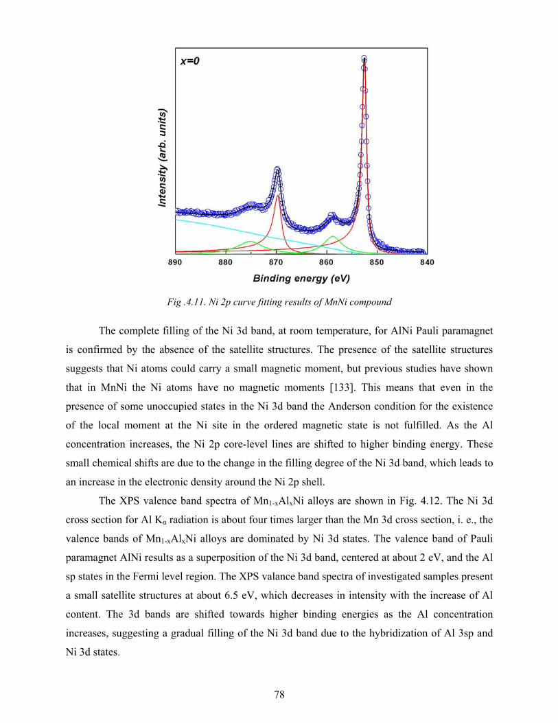
78

Fig .4.11. Ni 2p curve fitting results of MnNi compound

The complete filling of the Ni 3d band, at room temperature, for AlNi Pauli paramagnet

is confirmed by the absence of the satellite structures. The presence of the satellite structures

suggests that Ni atoms could carry a small magnetic moment, but previous studies have shown

that in MnNi the Ni atoms have no magnetic moments [133]. This means that even in the

presence of some unoccupied states in the Ni 3d band the Anderson condition for the existence

of the local moment at the Ni site in the ordered magnetic state is not fulfilled. As the Al

concentration increases, the Ni 2p core-level lines are shifted to higher binding energy. These

small chemical shifts are due to the change in the filling degree of the Ni 3d band, which leads to

an increase in the electronic density around the Ni 2p shell.

The XPS valence band spectra of Mn1-xAlxNi alloys are shown in Fig. 4.12. The Ni 3d

cross section for Al Kα radiation is about four times larger than the Mn 3d cross section, i. e., the

valence bands of Mn1-xAlxNi alloys are dominated by Ni 3d states. The valence band of Pauli

paramagnet AlNi results as a superposition of the Ni 3d band, centered at about 2 eV, and the Al

sp states in the Fermi level region. The XPS valance band spectra of investigated samples present

a small satellite structures at about 6.5 eV, which decreases in intensity with the increase of Al

content. The 3d bands are shifted towards higher binding energies as the Al concentration

increases, suggesting a gradual filling of the Ni 3d band due to the hybridization of Al 3sp and

Ni 3d states.

79

Fig .4.12. XPS valence band spectra of Mn1-xAlxNi alloys


Since the Ni atoms do not carry any magnetic moment [121, 133], the interaction Mn-Mn

is responsible for the magnetic properties of all investigated alloys.

The alloys Mn1-xAlxNi for x<0.4 are antiferromagnets with very high Néel temperatures,

namely 1073 K for MnNi [116], 1026 K for Mn0.9Al0.1Ni and 820 K for Mn0.8Al0.2Ni. For

illustration, in Fig. 4.13 is shown the temperature dependence of the measured magnetic

susceptibility for Mn0.9Al0.1Ni alloy. The distance between the nearest-neighbor Mn atoms in

these alloys, determined from XRD measurements, is about 2.64 Å. It is well known that the Mn-

Mn interaction is antiferromagnetic when the distance is smaller than 3 Å [134].

The magnetic field dependence of magnetization at different temperatures for x≥0.5

shows a small curvature (Fig. 4.14), suggesting the presence of a ferromagnetic phase L21, in

which the interaction between the Mn atoms is due to the RKKY coupling [135]. On the other

hand, the magnetization does not saturate even at B=10 T, what implies the existence in the

alloys of the antifferomagnetic B2 phase.

80

Fig.4.13. Susceptibility versus temperature of Mn0.9Al0.1Ni alloy. In the inset is shown the

thermal variation of the susceptibility for MnNi [116].

The alloys Mn1-xAlxNi for 0.4< x < 1 have complex mictomagnetic behavior, with a mixture of

antiferromagnetic and ferromagnetic interactions. The coexistence of antiferromagnetism and

ferromagnetism in Mn0.5Al0.5Ni alloy was also confirmed in the literature by the susceptibility

measurements in field cooled (FC) and zero field cooled (ZFC) [121].

81

Fig.4.14. Magnetic field dependence of magnetization, at different temperatures, of

Mn0.4Al0.6Ni, Mn0.2Al0.8Ni and Mn0.1Al0.9Ni alloys.

The hysteresis loops (see the insets) are shifted to lower negative fields, the effect being

more pronounced for x=0.6. The shift in the magnetization of a ferromagnetic component is due

to the exchange interaction between the antiferromagnet and ferromagnet at their interface. The

ferromagnetic component, which is strongly coupled with the antiferromagnetic one, has its

interfacial spins pinned. At lower Mn concentrations, i. e. x = 0.8 and x = 0.9, the amount of

antiferromagnetic component decreases (the probability to have Mn-Mn pairs becomes smaller),

what explains the almost symmetrical form of the hysteresis loop in this concentration range.

The coercive field at T = 5 K increases as Mn concentration decreases, from 0.05 T for x = 0.6 to

0.11 T for x = 0.9. The small values of the coercive field can be explained in the random

anisotropy model [136]. The increase of the coercive field as temperature decreases indicates

enhancement of the local magnetic anisotropy.

The coexistence of antiferromagnetism and ferromagnetism in Mn1-xAlxNi alloys for 0.6

≤ x < 1 is also revealed by the magnetic measurements in lower magnetic fields. In fig. 4.15 is

shown the temperature dependence of FC and ZFC susceptibilities in an applied field of 0.1T.

The distinguishing experimental feature of mictomagnetism is that the magnetization drops

abruptly at the freezing temperature Tf when the material is cooled in the absence of magnetic

field, resulting in a splitting of the FC and ZFC susceptibilities at a certain temperature. The

values of this temperature and also the freezing temperature are related to the dilution effect, like

in other mictomagnetic systems [137]. The exchange interactions of Mn-Mn type are partially

broken when Mn is substituted by Al. The increase of the ZFC susceptibility for x = 0.6 at low

temperatures was also observed for x=0.5 [121] and may be due to the conical antiferromagnetic

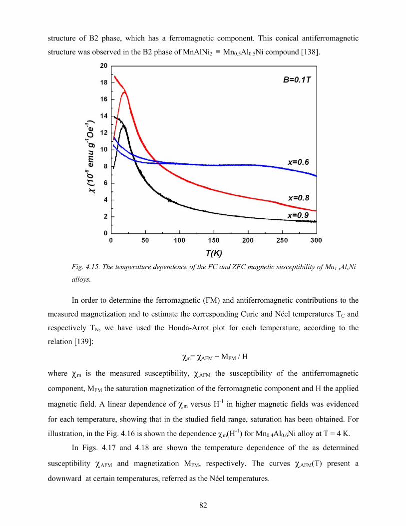
82

structure of B2 phase, which has a ferromagnetic component. This conical antiferromagnetic

structure was observed in the B2 phase of MnAlNi2 ≡ Mn0.5Al0.5Ni compound [138].

Fig. 4.15. The temperature dependence of the FC and ZFC magnetic susceptibility of Mn1-xAlxNi

alloys.

In order to determine the ferromagnetic (FM) and antiferromagnetic contributions to the

measured magnetization and to estimate the corresponding Curie and Néel temperatures TC and

respectively TN, we have used the Honda-Arrot plot for each temperature, according to the

relation [139]:

χm= χAFM + MFM / H

where χm is the measured susceptibility, χAFM the susceptibility of the antiferromagnetic

component, MFM the saturation magnetization of the ferromagnetic component and H the applied

magnetic field. A linear dependence of χm versus H-1 in higher magnetic fields was evidenced

for each temperature, showing that in the studied field range, saturation has been obtained. For

illustration, in the Fig. 4.16 is shown the dependence χm(H-1) for Mn0.4Al0.6Ni alloy at T = 4 K.

In Figs. 4.17 and 4.18 are shown the temperature dependence of the as determined

susceptibility χAFM and magnetization MFM, respectively. The curves χAFM(T) present a

downward at certain temperatures, referred as the Néel temperatures.

83

Fig. 4.16. The 1/H dependence of the χm for Mn0.4Al0.6Ni alloy at T = 4 K. In the inset is shown

the linear dependence at high magnetic fields (7-10) T

Fig. 4.17. The temperature dependence of the magnetic susceptibility χAFM of Mn1-xAlxNi

alloys. The arrows indicate the Néel temperatures.

84

Fig. 4.18. The temperature dependence of the magnetization MFM for Mn1-xAlxNi alloys.

At about the same temperatures T≈TN, the curves MFM(T) show a small anomaly in the

magnetization of the ferromagnetic component, due to the pinning effect. The Curie temperatures

TC have been determined in the molecular field approximation from the MFM2(T) dependence.

The as determined transition temperatures are given in Table 4.1.

Fig.4.19. Reciprocal susceptibility versus temperature of Mn1-xAlxNi alloys.

85

The thermal variation of the reciprocal magnetic susceptibility for the investigated alloys

in the high temperature range is shown in Fig. 4.19. The experimental data fit a Curie-Weiss law

with a small additional temperature-independent term χ0, in which the principal contribution is

brought by the Pauli susceptibility χP of the conduction electrons:

χ=C/(T-θ) + χ0

The values of the effective magnetic moments μeff and of the paramagnetic Curie

temperatures θ are given in Table 4.1. The Ni 3d band for x≥0.5 is almost filed. This assumption

is confirmed by the very small intensity of the Ni 2p and valence band satellite. The contribution

of the Ni atoms to the total effective magnetic moment is negligible, so the measured effective

magnetic moment may be attributed only to the Mn atoms. The effective magnetic moments per

Mn atom have approximately the same value, corresponding to a spin S≅2, like in the parent

compound MnNi, showing that the Mn 3d band is not affected by alloying, suggesting that the

hybridization between the Mn 3d states and the Al 3sp states is very small. The paramagnetic

Curie temperatures θ are much lower than the Curie temperatures TC. This is due to the

contribution of antiferromagnetic part in the measured magnetic susceptibility, which has a

negative θ value, and consequently an averaged paramagnetic Curie temperature is observed.

The relative proportion of the ferromagnetic and antiferromagnetic parts in the samples is also

reflected in the difference between the Curie temperatures TC and paramagnetic Curie

temperatures θ as a function of the Al content. This difference decreases with Al concentration,

confirming the decrease of the antiferromagnetic component at lower Mn concentrations.

Table. 4.1. Transition temperatures and effective magnetic moments of Mn1-xAlxNi alloys

*data taken from [121]

x TN (K) TC (K) θ (K) µeff (µB/f.u.) µeff (µB/Mn)

0.5 313* 375* 123 3.44 4.87

0.6 181 284 108 3.07 4.85

0.8 80 121 50 2.21 4.94

0.9 26 59 -3 1.55 4.90

86

4.4 Conclusions

The substitution of Al for Mn in MnNi leads to significant changes in the crystallographic

structure with remarkable effects on the magnetic properties and electronic structure of

Mn1-xAlxNi alloys.


moments on Mn sites in all Mn1-xAlxNi alloys.

The investigated alloys are antifferomagnets, but for x≥0.5 the antiferromagnetism (B2)

and ferromagnetism (L21) coexist.

The exchange interaction between the antifferomagnetic and ferromagnetic entities at

their interfaces leads to different configurational “pinning” of ferromagnetic components.

The transition temperatures decrease as Al concentration increases.

The hybridization between Ni 3d and Al 3sp states leads to a gradual filling of the Ni 3d

band.

The Mn 3d band in Mn1-xAlxNi system is not affected by alloying.

87

Chapter 5

Electronic structure and magnetic properties of Ni1-xMnxAl alloys [140-142]

In the previous two chapters it was studied the influence of the substitution of Mn by Al

in the ternary system Al-Mn-Ni, on the electronic, crystallographic and magnetic structure,

keeping the Ni atomic concentration constant. In the present chapter the Al atomic concentration

will remain the same and we will focus on the effect of the substitution of Ni by Mn.

The phase diagram (Fig. 5.1) indicates, in case of Ni1-xMnxAl system, a large region of

solid solubility, excepting for the high Mn concentrations. There are no reports about bulk AlMn

in a stable phase, but only on Al0.89Mn1.11 [143]. In the other side of the concentration range is

AlNi, a Pauli paramagnet.


Magnetic properties of the Ni1-xMnxAl alloys were reported in literature [144], but there

are no explanation regarding the relative small values of the measured magnetic moments per

atom, their variation with Ni atoms concentration and if Ni brings or not a contribution in the

measured magnetic moments.

88

The aim of this chapter is to explain the magnetic properties of the investigated alloys by

correlating the magnetic measurements, in the ordered and paramagnetic state, with XRD and

XPS results.


Seven samples from the Ni1-xMnxAl system (x=0.0, 0.2, 0.3, 0.4, 0.5, 0.6, 0.8) were


samples. The broad character of the peaks indicates the presence of the strains in the samples. X-

ray diffraction pattern of Ni1-xMnxAl alloys are shown in Fig. 5.2.

Fig. 5.2. X-ray diffraction pattern of Ni1-xMnxAl alloys.

All the investigated alloys are single phases with the same CsCl (B2) structure type (Fig. 5.3a).

The lattice parameter, estimated using the Powder Cell program, increases monotonically with

Mn concentration from a=2.875 Å for NiAl to a=2.966 Å for Ni0.2Mn0.8Al (Fig. 5.3b).

89

Fig.5.3. Elementary cell of Ni1-xMnxAl alloys (a) and the variation of the lattice

parameter with Mn content (b)

5.2 XPS Spectra The XPS valence band spectra of investigated alloys are shown in Fig. 5.4. The

maximum of the Ni 3d band is shifted to a BE of 1.8 eV comparing to the value of 0.6 eV in pure

metallic Ni [122]. The shoulder near Fermi level is due to the Al 3sp states. Another contribution

to the XPS valence band spectra of Ni1-xMnxAl alloys comes from Mn 3d states, which are

concentrated at the bottom of the VB in the 2.5-3eV BE region, as previously demonstrated by

band structure calculation and experimental measurements for many alloys and intermetallic

compounds based on Mn [109-111]. There is also an appreciable hybridization between the Mn

3d and Al 3sp states which leads, according Mn 3s XPS spectra and magnetic measurements, to a

partial filling of the Mn 3d band.

Fig .5.4. XPS valence band spectra of Ni1-xMnxAl alloys

90

The Ni 2p spectra for all investigated alloys are situated at the same BE, but are shifted to

higher BE relative to pure metallic Ni. This also confirms the partial filling of Ni 3d band. The

first vicinity of Ni atoms in the Ni1-xMnxAl alloys does not change by alloying, what explains the

lack of the chemical shift in the Ni 2p spectra.

Fig .5.5. Ni 2p XPS spectra of Ni1-xMnxAl alloys and pure metallic Ni

In Ni metal the Ni 2p satellite structure, situated at about 6.5 eV higher BE energy, is an

evidence for unoccupied 3d states. The intensity of the satellites in Ni1-xMnxAl alloys is

drastically reduced (see Fig. 5.5) confirming the partial filling of the Ni 3d band of the

investigated alloys, except for x=0 where the satellite structure disappears. This confirms the

previous magnetic measurements that have shown that NiAl is a Pauli paramagnet with Ni 3d

band completely filled, at room temperature, due to the hybridization with Al 3sp states.

The Mn 3s core level spectra show an exchange splitting around 4 eV arising from the

exchange interactions between the core hole and the open 3d shell. The exchange splitting in

MnNi is about 5.2 eV and the Mn magnetic moment is about 4 µB/Mn [116]. The exchange

splitting is proportional with the Mn local moment [122]. Fig. 5.6 presents the curve fitting

results of Mn0.8Ni0.2Al alloy, after background subtraction, and the similar spectrum of MnNi

compound.

91

Fig. 5.6. Mn 3s curve fitting results of Mn0.8Ni0.2Al alloy and MnNi compound


The values of the spontaneous magnetization, for each temperature, were determined

from M(H) curves by extrapolation the linear dependence at H→0. The temperature dependence

of the spontaneous magnetization of Ni1-xMnxAl alloys is shown in Fig. 5.7.

Fig. 5.7. Temperature dependence of spontaneous magnetization of Ni1-xMnxAl alloys

92

The values and variations of magnetization with magnetic field (Fig. 5.8) and temperature

suggest that all the investigated alloys have a ferromagnetic behavior, below the corresponding

Curie temperatures.

Fig. 5.8. Magnetic field dependence of magnetization at T=4K of Ni1-xMnxAl alloys.

The Curie temperatures TC have been determined in the molecular field approximation from the

MFM2(T) dependence (Fig. 5.9). The values are given in Table 5.1.

Fig. 5.9. MFM

2 as a function of temperature of Ni1-xMnxAl alloys

93

The thermal variation of the reciprocal magnetic susceptibility for the investigated alloys

in the high temperature range is shown in Fig. 5.10. The experimental data fit a Curie-Weiss law

with a small additional temperature-independent term χ0, in which the principal contribution is

brought by the Pauli susceptibility χP of the conduction electrons:

χ=C/(T-θ) + χ0

The values of the effective magnetic moments μeff and of the paramagnetic Curie

temperatures θ are given in Table 5.1. As one can see from Fig. 5.10, the contribution of χ0 is

more pronounced in the measured magnetic susceptibility for smaller Mn concentrations.

Fig.5.10. Reciprocal susceptibility versus temperature of Ni1-xMnxAl alloys. In the inset is given the

temperature dependence of magnetic susceptibility of NiAl [145]

The magnetic susceptibility of NiAl does not depend on temperature in the region 80-

100K and has the value: gemumeasNiAl /10265.0 6−×=χ [145]. There are three contributions to the

total measured susceptibility: diaLmeasp

measNiAl χχχχ ++= , where meas

pχ is the measured Pauli

susceptibility of conduction electrons, Lχ the Landau diamagnetism of the conduction electrons

and diaχ the diamagnetism of the atomic cores. The Pauli susceptibility in the free electrons

94

approximation is given by: 63/13/2

60 103.01086.1 −− ×=⎟⎟⎠

⎞⎜⎜⎝

⎛×= nM

p ρχ emu/g, where M is the

molecular mass, ρ the density and n the number of s, p and d valence electrons per unit

formula. The Landau diamagnetism is 60 101.031 −×−=−= pL χχ emu/g. The diamagnetic

contribution to the magnetic susceptibility is 61018.0 −×−=+= Nidia

Aldiadia χχχ emu/g [145]. The

measured Pauli susceptibility is 610545.0 −×=−−= diaLmeasNiAl

measp χχχχ emu/g. The ratio

0p

measp

χχ

δ = between the between the Pauli susceptibilities of d electrons measured and calculated

in the free electron approximation is the Stoner enhancement factor which for NiAl has the value

8.1=δ . This value shows that NiAl is exchange-enhanced Pauli paramagnet, suggesting that

also the Ni1-xMnxAl alloys could be exchange-enhanced Pauli paramagnets, which are correctly

treaded in the self-consistent renormalization (SCR) theory of spin fluctuations [34].

Table 5.1. The magnetic moments in the ordered (µ) and paramagnetic state (µeff), the Curie

(TC) and paramagnetic Curie (θ) temperatures and the lattice constants (a) of the Ni1-xMnxAl

alloys.

µ (µB/f.u.) µeff (µB/f.u.) TC (K) θ (K) a (Å) x=0 2.8752

x=0.2 0.19 1.06 367 385.7 2.8919 x=0.3 0.34 1.57 379.8 395 2.906 x=0.4 0.51 1.9 381.5 398.8 2.9155 x=0.5 0.77 2.32 385 405.5 2.927 x=0.6 1.01 2.66 401 422.7 2.9356 x=0.8 1.24 2.9 420.8 445.9 2.9664

TC and θ increase monotonically with Mn concentration in good agreement with the

theory of ferromagnetic materials, TC being proportional with the number Z of neighboring

magnetic atoms [146]. Comparing the intensity of the Ni 2p and valence band satellites in this

systems with the similar ones in the previous system Mn1-xAlxNi, one may conclude that also in

Ni1-xMnxAl alloys the Anderson condition of the existance of a local moment on Ni sites in the

ordered state is not fulfilled. So, the measured magnetic moments in the ordered state are

attributed to Mn atoms only. The values of the Mn spins SMn (see Table 5.2) were obtained from

the relation µMn =2 SMnµB. Using these values, the effective Mn magnetic moments are calculated

95

( BMnMnMneff SS μμ )1(2 += ). In the paramagnetic region we have to consider the contribution of

Ni magnetic moments, induced by temperature, to the magnetic susceptibility (the Ni 3d band is

not completely filled). In the last column the Ni contribution to the effective magnetic moment is

calculated ( 222.. NiMnuf yx μμμ += , x and y are the molar fraction of Mn and Ni, respectively). The

Ni effective magnetic moment has reasonable values for x≤0.4, comparable with the values on

Ni sites in other spin fluctuation systems [147, 148]. For x>0.4 the calculated Ni effective

magnetic moments are too large; this suggests that not all the Mn atoms moments are orientated

in the same direction and is possible to have antiferromagnetic Mn-Mn pairs. The probability of

the apparition of Mn-Mn antiferromagnetic pairs increases with Mn concentrations.

Table 5.2. The magnetic moments and spin of Mn atoms in the ordered state and the

calculated Mn and Ni effective magnetic moments of the Ni1-xMnxAl alloys.

Mnordμ SMn

Mneffμ

x=0.2 0.95 0.48 1.69 x=0.3 1.13 0.57 1.89 x=0.4 1.28 0.64 2.05 x=0.5 1.54 0.77 2.33 x=0.6 1.68 0.84 2.49 x=0.8 1.55 0.78 2.36

The strong Mn 3d - Al 3sp hybridization is due to the high number of Al atoms in the Mn

first vicinity, namely 8 Al atoms at ~2.5 Å. This explains the small values of the Mn magnetic

moments in Ni1-xMnxAl alloys comparing to MnNi. The Mn magnetic moment in the ordered

state increases with Mn concentration, except for the x=0.8 alloy. This variation can be

associated with the increase of the lattice parameter which leads to a decreasing in the Mn 3d -

Al 3sp hybridization degree. But together with the Mn concentration, increases also the

probability of the Mn-Mn antiferromagnetic pairs formation, so that a number of Mn magnetic

moments do not contribute to the magnetization. These two phenomena influence the value of

the measured magnetic moments.

It is well known that Mn-Mn interaction is antiferromagnetic when the distance is smaller

than ~2.9 Å [29], comparable with the lattice constant in Ni1-xMnxAl alloys. For larger values the

coupling is ferromagnetic. In these alloys there are two possibilities for the appearance of

antiferromagnetic Mn-Mn pairs:

96

• There are two Mn atoms in the centre of near neighbour cells and lattice parameter is

smaller than 2.9 Å (Fig. 5.11 a);

• A crystallographic disorder appears: Mn and Al atoms switch places, thus the Mn-Mn

distance became ~2.5 Å (Fig. 5.11 b). The problem of crystallographically disorder alloys

was fully discussed in chapter 3.

Fig. 5.11. Possible situations for Mn-Mn distance smaller than 2.9 Å

5.4 Conclusions

The substitution of Ni for Mn in NiAl leads to no significant changes in the

crystallographic structure, but has remarkable effects on the magnetic properties and

electronic structure of Ni1-xMnxAl alloys.

Ni1-xMnxAl alloys present a ferromagnetic behaviour below the corresponding Curie

temperatures.

The correlation between the results from ordered and paramagnetic state indicates the

presence of some antiferromagnetically Mn-Mn pairs.

97

The temperature dependence of the reciprocal susceptibility may be explained in terms of

the self-consistent renormalization theory of spin fluctuations.

Ni 3d band is partially filled due to the hybridization with Al 3sp states.

The strong hybridization between Mn 3d and Al 3sp states is responsible for the lower

values of the Mn magnetic moments.

98

Chapter 6

Electronic structure and magnetic properties of Ni0.7-xAlxMn0.3 alloys [149]

In the last three chapters it was presented the effect of the substitution of Mn by Al atoms

and Ni by Mn atoms in the electronic, crystallographic and magnetic structure, keeping the Ni

and respective Al atomic concentration constant. To have a complete picture of the Al-Mn-Ni

system in this chapter the Mn atomic concentration will remain the same and the substitution

effect of Ni by Al atoms will be studied.

The phase diagram (Fig. 6.1) indicates, in case of Ni0.7-xAlxMn0.3 alloys, two main regions

of solid solubility. There are no reports in the literature regarding the structure, magnetic and

spectroscopic properties of Ni0.7-xAlxMn0.3 system.


99


Seven samples from the Ni0.7-xAlxMn0.3 system (x=0.0, 0.1, 0.2, 0.3, 0.4, 0.5, 0.7) were


samples. X-ray diffraction pattern of Ni0.7-xAlxMn0.3 alloys are shown in Fig. 6.2. The broad

character of the peaks indicates the presence of the strains in the samples.

Fig. 6.2. X-ray diffraction pattern of Ni0.7-xAlxMn0.3 alloys

All the investigated alloys are single phases except for Al0.7Mn0.3 and Ni0.5Al0.2Mn0.3 alloys.

XRD measurements revealed a change in the crystallographic structure around x = 0.2 from

AuCu3 to CsCl (B2) structure type. Ni0.5Al0.2Mn0.3 appears as a mixture of these two structures.

The results only from the single phase alloys are presented in the following pages.

Fig.6.3.Representation of AuCu3 and ClCs structure type

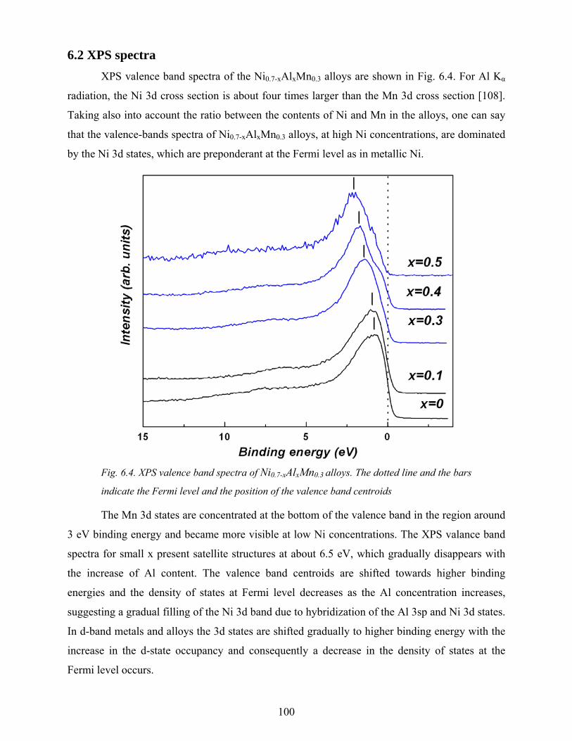
100

6.2 XPS spectra

XPS valence band spectra of the Ni0.7-xAlxMn0.3 alloys are shown in Fig. 6.4. For Al Kα

radiation, the Ni 3d cross section is about four times larger than the Mn 3d cross section [108].

Taking also into account the ratio between the contents of Ni and Mn in the alloys, one can say

that the valence-bands spectra of Ni0.7-xAlxMn0.3 alloys, at high Ni concentrations, are dominated

by the Ni 3d states, which are preponderant at the Fermi level as in metallic Ni.

Fig. 6.4. XPS valence band spectra of Ni0.7-xAlxMn0.3 alloys. The dotted line and the bars

indicate the Fermi level and the position of the valence band centroids

The Mn 3d states are concentrated at the bottom of the valence band in the region around

3 eV binding energy and became more visible at low Ni concentrations. The XPS valance band

spectra for small x present satellite structures at about 6.5 eV, which gradually disappears with

the increase of Al content. The valence band centroids are shifted towards higher binding

energies and the density of states at Fermi level decreases as the Al concentration increases,

suggesting a gradual filling of the Ni 3d band due to hybridization of the Al 3sp and Ni 3d states.

In d-band metals and alloys the 3d states are shifted gradually to higher binding energy with the

increase in the d-state occupancy and consequently a decrease in the density of states at the

Fermi level occurs.

101

The Ni 2p core-level spectra of Ni0.7-xAlxMn0.3 alloys are shown in Fig. 6.5. The Ni 2p3/2

core level spectra exhibit satellite structures at about 6.5 eV higher binding energy (Fig. 6.6).

Fig .6.5. Ni 2p XPS spectra of Ni0.7-xAlxMn0.3 alloys

As the Al concentration increases, the Ni 2p core-level lines are shifted to higher binding

energy. These small chemical shifts are due to the change in the filling degree of the Ni 3d band,

which leads to an increase in the electronic density around the Ni 2p shell.

102

Fig .6.6. Ni 2p curve fitting results of Ni0.7-xAlxMn0.3 alloys and the Al concentration

dependence of Ni 2p3/2 satellite area

The observation of satellites implies the presence of d character in the unoccupied bands.

The satellite structure intensity decreases as the Al content increases, confirming the gradual

filling of the Ni 3d band. The presence of the satellite structures suggests that Ni atoms could

carry a small magnetic moment.


The observed spin orbit splitting, which can be identified in the distance between the two centers

of energy of the 2p3/2 and 2p1/2 state is Δso≈11.5 eV.

103

Fig .6.7. Mn 2p XPS spectra of Ni0.7-xAlxMn0.3 alloys and Ni Auger line

After background removal, using a Shirley-type background shape, we have also fitted

the Mn 2p3/2 core-level spectra for some of the investigated alloys with four components and a

satellite line situated at binding energy around 644.5 eV. The curve fitting results for Ni0.7Mn0.3

alloy is given in Fig. 6.8, with the mean energy separation Δex≈1.2 eV. This gives direct evidence

of the existence of local moments confined on Mn sites.

Fig. 6.8. Mn 2p3/2 curve fitting results of Ni0.7Mn0.3 alloy

104


The temperature dependence of magnetic susceptibility of Ni0.7Mn0.3 and Ni0.4Al0.3Mn0.3

alloys is given in Fig. 6.9. The susceptibility presents a maximum, specific for antiferromagnetic

materials, which corresponds to Néel temperature. The values of the transition temperature are

TN≈150K and TN≈125K for Ni0.7Mn0.3 and Ni0.4Al0.3Mn0.3, respectively.

Fig. 6.9. The temperature dependence of magnetic susceptibility of Ni0.7Mn0.3 and Ni0.4Al0.3Mn0.3 alloys

The increase of the magnetic susceptibility at very low temperatures could be due to some

ferromagnetic impurity or a conical antiferromagnetic structure, which has a ferromagnetic

component. This feature was also observed in the Chapter 4.

The spontaneous magnetization as a function of temperature is given in Fig. 6.10 for

Ni0.6Al0.1Mn0.3 and Ni0.3Al0.4Mn0.3 alloys. The small values of spontaneous magnetization

suggest a ferrimagnetic behavior of these two alloys.

Fig. 6.10. The temperature dependence of the spontaneous magnetization of Ni0.6Al0.1Mn0.3 and

Ni0.3Al0.4Mn0.3 alloys

105

Fig. 6.11 shows the temperature dependence of the reciprocal susceptibility of

Ni0.6Al0.1Mn0.3 and Ni0.3Al0.4Mn0.3 alloys in the paramagnetic state. The reciprocal of magnetic

susceptibility follows a Néel-type hyperbolic law, specific to ferrimagnetic materials. Usually for

ferromagnetic materials, the high temperature asymptote to the hyperbola has a Curie-Weiss

form. Unfortunately, for these two alloys, because the transition temperature is very high and the

instrumentation upper limit temperature was around 900K, the asymptote to the hyperbola was

not reached.

Fig. 6.11. The temperature dependence of the reciprocal susceptibility of Ni0.6Al0.1Mn0.3 and

Ni0.3Al0.4Mn0.3 alloys

The Curie temperatures TC have been determined in the molecular field approximation from the

MFM2(T) dependence (Fig. 6.12) and have the values 780.5K and 645K for Ni0.6Al0.1Mn0.3 and

Ni0.3Al0.4Mn0.3, respectively.

106

Fig. 6.12. MFM2 as a function of temperature of Ni0.6Al0.1Mn0.3 and Ni0.3Al0.4Mn0.3 alloys

The values and the variation of the magnetic susceptibility with the temperature (Fig.

6.13a) suggest a ferromagnetic behavior of Ni0.2Al0.5Mn0.3 alloy. The ferromagnetic Curie

temperature, determined in the same way like above, has the value TC=400K. The reciprocal

susceptibility as a function of temperature for Ni0.2Al0.5Mn0.3 alloy is presented in Fig. 6.13b and

confirms the ferromagnetic behavior. The experimental data fit a Curie-Weiss law.

Fig. 6.13. The spontaneous magnetization (a), and the reciprocal magnetic susceptibility (b) as a function

of temperature of Ni0.2Al0.5Mn0.3 alloy

The magnetic behavior of Ni0.7-xAlxMn0.3 alloys is illustrated in Fig. 6.14. We have seen

in the Chapter 3 that in the ordered AuCu3 structure type, Mn and Al atoms occupy the 1a

position and Ni atoms are situated in 3c position. In this case the coupling between the Mn atoms

107

is ferromagnetic (dMn-Mn>2.9A°). In the crystallographically disordered alloys a number of Mn

atoms occupy the 3c positions and generate antiferromagnetic Mn-Mn pairs with the Mn atoms

from their firs vicinity situated in 1a or 3c positions (dMn-Mn<2.9A°). In AuCu3 structure type

25% of atoms will occupy the 1a position and 75% the 3c position. On can see that in Ni0.7Mn0.3

alloy even if the disorder degree is considered to be zero, a number of Mn atoms will be forced

to take the 3c position and to form Mn-Mn antiferromagnetic pairs. Furthermore, at this Mn

concentration the alloy is crystallographically disordered (see Chapter 3), with a disorder degree

very high. This explain the magnetic measurements results, which shown that Ni0.7Mn0.3 alloy

has antiferromagnetic behavior.

In the Chapter 3 we have also seen that Al atoms play an important role in the stability of

the crystallographically ordered structures, and the probability of the apparition of

antiferromagnetic Mn-Mn pair decrease with the increase of Al concentration. This explains why

Ni0.6Al0.1Mn0.3 alloy has a ferrimagnetic behavior.

Fig. 6.14. The magnetic behavior of Ni0.7-xAlxMn0.3 alloys

The Ni0.4Al0.3Mn0.3 alloy has the lattice parameter a≈2.90Å. At this distance the Mn-Mn

coupling is antiferromagnetic. The Ni0.3Al0.4Mn0.3 alloy has the lattice parameter a little bit larger

a≈2.914Å, but seems to be at the limit distance between the AFM and FM coupling. This could

be a reason why this alloy has ferrimagnetic behavior. The lattice parameter of the

Ni0.2Al0.5Mn0.3 alloy is larger (a≈2.94) and it has a ferromagnetic behavior. This means that at

this distance the coupling between the Mn atoms is parallel.

6.4 Conclusions

The substitution of Al for Ni leads to significant changes in the crystallographic structure

with remarkable effects on the electronic structure of Ni0.7-xAlxMn0.3 alloys.

108

XPS spectra pointed out the existence of local magnetic moments on Mn sites in Ni0.7-

xAlxMn0.3 alloys.

Ni 2p core-level spectra evidenced the existence of unoccupied 3d states, which is one of

the conditions for the apparition of local magnetic moments at Ni sites.

The hybridization between the 3d Ni and 3sp Al states leads to a partial filling of the Ni

3d band, as indicated by the XPS core level and valence band spectra.

At low Al concentrations the crystallographic structure remains the same but a change in

the magnetic structure appears once Ni atoms are substituted by Al atoms. Aluminium

plays an important role in stabilizing the crystallographic ordered structure.

In the case of Ni0.7-xAlxMn0.3 alloys, with ClCs structure type, a transition from

antiferromagnetic to ferromagnetic through an intermediate ferrimagnetic behavior was

evidenced once the Al concentration increases.

This system is a very good example of how one can change the crystallographic structure

type, the electronic structure and the magnetic interactions between the local magnetic

moments by changing the atomic concentration of the constituents.

109

Summary

The main idea of the thesis was to see how one can change the crystallographic structure

type, the electronic structure, the values of the magnetic moments and the sign of the interactions

between the local magnetic moments by changing the atomic concentration of the constituent

atoms in the ternary system Al-Mn-Ni.

The magnetic properties of the investigated alloys and compounds are strongly correlated

with their crystallographic properties and reflect the changes in the first vicinity and in the

distances between the 3d atoms. By changing the stoichiometry one can change the

crystallographic structure type (Mn1-xAlxNi and Ni0.7-xAlxMn0.3 systems), but even if the

crystallographic structure remains the same (Mn1-xAlxNi3 and Ni1-xMnxAl) the variation in the

lattice parameters leads to changes in the coupling between the magnetic moments of 3d

elements.

Some of the Al-Mn-Ni alloys are crystallographically disordered, but the crystallographic

disorder degree decreases quickly with the increase of Al concentration. Aluminum plays an

important role in stabilizing the crystallographic ordered structure in Mn1-xAlxNi3 alloys. The

same effect was observed for Ni0.7-xAlxMn0.3 in the small range of Al concentrations.


moments confined to the Mn sites for all Mn-Ni-Al alloys and compounds.

The hybridization between 3d Ni and 3sp Al states leads to a partial or complete filling of

Ni 3d band, as indicated by XPS core level and valence band spectra.

XPS and magnetic measurements evidenced that Mn 3d band in Mn1-xAlxNi3 and

Mn1-xAlxNi systems is not affected by hybridization with Al 3sp states while in Ni1-xMnxAl and

Ni0.7-xAlxMn0.3 systems Mn 3d band is strongly affected. This depends again on the interatomic

distances.

XPS spectra suggest that Ni atoms could carry small magnetic moments in almost all the

investigated alloys but, the Anderson condition for the existence of a local magnetic moment at

Ni sites, in the ordered magnetic state, is fulfilled only for Mn1-xAlxNi3 alloys. Ni atoms bring

their contribution to the effective magnetic moment in the paramagnetic state. In many cases

their contribution is small but for some of the investigated alloys temperature induced spin

fluctuations at Ni sites were evidenced.

110

Magnetic measurements revealed different types of magnetic ordering: ferromagnetic,

ferrimagnetic, antiferromagnetic and in some of the investigated alloys coexistence between

antiferromagnetism and ferromagnetism was evidenced. By changing the stoichiometry was

possible to pass from one type of magnetic ordering to another. A very good example is the

Ni0.7-xAlxMn0.3 system, where a transition from antiferromagnetism to ferromagnetism through an

intermediate ferrimagnetic phase was evidenced once the Al concentration increases.

The profound understanding of the magnetic phenomena and the correct interpretation of

the magnetic properties of the alloys and intermetallic compounds based on transition elements

can be achieved only through the correlation of obtained data from XPS, XRD and magnetic

measurements, corroborated with the band structure calculations.

111

References [1] P.O.M. Dirac, Proc. Roy. Soc. Lond. A 123 (1929) 714-733 [2] J.H. Van Vleck, in "The Theory of Electric and Magnetic Susceptibilities", Oxford University Press,

Oxford, 1932 [3] W. Heisenberg, Z. Physik 38 (1926) 411 [4] H.A. Kramers, Physica 1 (1934) 825-828 [5] P.W. Anderson, Phys. Rev. 115 (1959) 2-13; Solid State Physics 14 (1963) 99 [6] P. Weiss, J. Phys. Radium 6 (1907) 661 [7] W. Heisenberg, Z. Physik 49 (1928) 619 [8] E.C. Stoner, Proc. Roy. Soc. A 165 (1938) 372-414 [9] J. F. Janak, Phys. Rev. B 16 (1977) 255-262 [10] J.H. Van Vleck, Rev. Mod. Phys. 25 (1953) 220-227 [11] P.W. Anderson, Phys. Rev. 124 (1961) 41-53 [12] J. Friedel, Can. J. Phys. 34 (1956) 1190; Nuovo Cimento Suppl. 7 (1958) 287 [13] S. Alexander and P.W. Anderson, Phys. Rev. 133 (1964) A1594-A1603 [14] T. Moriya, Prog. Theor. Phys. 33 (1965) 157; In “Theory of Magnetism in Transition Metals”, Proc.

Int. School of Phys. Enrico Fermi, vol.37, ed. by W. Marshall, Academic, New York, 1967, p.206 [15] Y. Ishikawa, Physica B 91 (1977) 130 [16] A. Hamzic, R. Asomoza, and I.A. Campbel, J. Phys. F 11 (1981) 1441 [17] Y. Noda and Y. Ishikawa, J. Phys. Soc. Jpn. 40 (1976) 690-698 [18] K. Tajima, Y. Ishikawa, P.J. Webster, M.W. Stringfellow, O. Tochetti, and K.R.A. Ziebeck, J. Phys.

Soc. Jpn. 43 (1977) 483-489 [19] K.R.A. Ziebeck, P.J. Webster, P.J. Brown, and J.A.C. Bland, J. Magn. Magn. Mater. 24 (1981) 258-

266 [20] K.R.A. Ziebeck and P.J. Brown, J. Phys. F10 (1980) 2015-2024 [21] D.M.K. Paul and W. G. Stirling, J. Phys. F: Met. Phys. 9 (1979) 2439-2449 [22] Y. Ishikawa, J. Magn. Magn. Mater. 14 (1979) 123-132 [23] J.W. Cable, E.O. Wollan, W.C. Koehler, and H.R. Child, Phys. Rev. 128 (1962) 2118-2120 [24] E. Krén, G. Kádár, Phys. Lett., 29A (1969) 340-341 [25] A. J. Smith, W. G. Stirling and T. M. Holden, J. Phys. F 7 (1977) 2411-2420 [26] H. Yamada and M. Shimizu, J. Phys. F 7 (1977) L203-L209 [27] M. Kohgi and Y. Ishikawa, J. Phys. Soc. Jpn. 49 (1980) 985-993; J. Phys. Soc. Jpn. 49 (1980) 994-

999 [28] K. R. A. Ziebeck, P. J. Brown, J. Deportes, D. Givord, P. J. Webster, J. G. Booth, Helv. Phys. Acta

56 (1983) 117 [29] A. Kjekshus, R. Mollebud, A.F. Andresen, and W.B. Pearson, Phil. Mag. 16 (1967) 1063 [30] T. Moriya, J. Magn. Magn. Mater. 31-34 (1983) 10-19 [31] B. T. Matthiss, R. M Bozorth, Phys. Rev. 100 (1958) 604 [32] B T. Matthias, A. M. Clogston, H. J. Williams, E. Corenzwit, R. C. Sherwood: Phys. Rev.

Lett. 7 (1961) 7 [33] T. Moriya, A. Kawabata, J. Phys. Soc. Jpn. 34 (1973) 639; 35 (1973) 669 [34] T. Moriya, Spin Fluctuations in Itinerant Electron Magnetism, (Springer-Verlag, Berlin, 1985) [35] W. Hallwachs, “Über den Einfluß des Lichtes auf elektrostatisch geladene Körper,” Wiedemann’sche Annalen, vol. 33, pp. 301–312, 1888 [36] H. Hertz, “Über den Einfluß des ultravioletten Lichtes auf die elektrische Entladung,” Wiedemann’sche Annalen, vol. 31, pp. 983–1000, 1887 [37] J. J. Thomson, “Cathode Rays,” Philosophical Magazine, vol. 44, pp. 293–316, 1897 [38] A. Einstein, “Über einen die erzeugung und verwandlung des lichtes betreffenden heuristichen gesichtspunkt,” Annalen der Physik, vol. 17, pp. 132–148, 1905 [39] C. N. Berglund andW. Spiecer, “Photoemission studies of copper and silver: Theory,” Physica Review, vol. 136, pp. A1030–A1044, 1964

112

[40] K. Siegbahn, C. Nordling, A. Fahlman, R. Nordberg, K. Hamrin, J. Hedman, G. Johansson, T. Bergmark, S. E. Karlson, I. Lindgren, and B. Lindberg, ESCA–Atomic, Molecular and Solid State Structure Studied by Means of Electron Spectroscopy. Almquist and Wicksell, Uppsala, 1967 [41] K. Siegbahn, C. Nordling, G. Johansson, J. Hedman, P. F. Heden, K. Hamrin, U. Gelius, T. Bergmark, L. O. Werme, R. Manne, and Y. Baer, ESCA Applied to Free Molecules. North Holland, Amsterdam, 1969 [42] K. Siegbahn, D. Hammond, H. Fellner-Feldegg, and E. F. Barnett, “Electron spectroscopy with monochromatized X–rays,” Nature, vol. 176, pp. 245–252, 1972 [43] H. P. Bonzel and C. Client, “On the history of photoemission,” Progress in Surface Science, vol. 49, pp. 107–153, 1995 [44] G. Ertl and J. Küppers, Low Energy Electrons and Surface Chemistry. VCH, Weinheim, 1985 [45] S. Hufner, Photoelectron spectroscopy. Springer–Verlag, Berlin, 1995 [46] C. Fadley, “Basic Concepts of X-ray Photoelectron Spectrocopy,” in Electron Spectroscopy: Theory, Techniques and Applications (C. Brundle and P. Backer, eds.), vol. 2, pp. 2–156, Academic Press, London, 1978 [47] C. Cohen-Tannoudji, B. Diu, and F. Laloë, Quantenmechanik, vol. 2. Walter de Gruyter, Berlin, 1999 [48] G. Borstel, “Theoretical aspects of photoemission,” Applied Physics A, vol. 38, pp. 193–204, 1985 [49] W. Nolting, “Influence of electron correlations on auger electron – and appearance potential – spectra of solids,” Zeitschrift für Physik – Condensed Matter, vol. 80, pp. 73–86, 1990 [50] J. C. Fuggle, R. Lässer, O. Gunnarsson, and K. Schönhammer, “Plasmon Gains as a Monitor of Incomplete Relaxation, Interference Effects, and the Transition from Sudden to Adiabatic Limits in Electron Spectroscopies,” Physical Review Letters, vol. 44, pp. 1090–1093, 1980 [51] J. D. Lee, O. Gunnarsson, and L. Hedin, “Transition from the adiabatic to the sudden limit in core-level photoemission: A model study of a localized system,” Physical Review B, vol. 60, pp. 8034–8049, 1999 [52] T. Koopmans, “Über die Zuordnung von Wellenfunktionen und Eigenwerten zu den eizelnen Elektronen eines Atoms,” Physica, vol. 1, pp. 104–113, 1933 [53] R. J. Powell and W. E. Spicer, “Optical properties of NiO and CoO,” Physical Review B, vol. 2, pp. 2182–2193, 1970 [54] C. Powell, “Attenuation lenghts of low–energy electrons in solids,” Surface Science, vol. 44, pp. 29–46, 1974 [55] J. C. Shelton, “Inelastic mean free paths for electrons in bulk jellium,” Surface Science, vol. 44, pp. 305–309, 1974 [56] H. Bethe, “Zur Theorie des Durchgangs schneller Korpuskulastrahlung durch Materie,” Annalen der Physik, vol. 5, pp. 325–400, 1930 [57] S. Tanuma, C. J. Powell, and D. R. Penn, “Proposed formula for electron inelastic mean free paths based on calculations for 31 materials,” Surface Science, vol. 192, pp. L849–L857, 1987 [58] S. Tanuma, C. J. Powell, and D. R. Penn, “Calculations of inelastic mean free paths for 31 materials,” Surface and Interface Analysis, vol. 11, pp. 577–589, 1988 [59] J. C. Ashley, “Interaction of low–energy electrons with condensed matter: stopping powers and inelastic mean free paths from optical data,” Journal of Electron Spectroscopy and Related Phenomena, vol. 46, pp. 199–214, 1988 [60] S. Tanuma, C. J. Powell, and D. R. Penn, “Calculations of inelastic mean free paths: II. Data for 27 elements over 50–2000 eV range,” Surface and Interface Analysis, vol. 17, pp. 911–926, 1991 [61] S. Tanuma, C. J. Powell, and D. R. Penn, “Calculations of inelastic mean free paths: III. Data for 15 inorganic compounds over 50–2000 eV range,” Surface and Interface Analysis, vol. 17, pp. 927–939, 1991 [62] S. Tanuma, C. J. Powell, and D. R. Penn, “Calculations of electron inelastic mean free paths (IMFPs): IV. Evaluation of calculated of calculated IMFPs formula TPP–2 for electron energies between 50 and 2000 eV,” Surface and Interface Analysis, vol. 20, pp. 77–89, 1993 [63] S. Tanuma, C. J. Powell, and D. R. Penn, “Calculations of inelastic mean free paths: V. Data for 14 organic compounds over 50–2000 eV range,” Surface and Interface Analysis, vol. 21, pp. 165–176, 1993

113

[64] A. Jablonski, “Universal energy dependence of the inelastic mean free path,” Surface and Interface Analysis, vol. 20, pp. 317–321, 1993 [65] J. Pendry, “Theory of Photoemision,” Surface Science, vol. 57, pp. 679–705, 1976 [66] D. J. Spanjaard, D. W. Jepsen, and P. M. Marcus, “Effects of transmission factors and matrix elements on angular distribution of photoemission from Ag(111),” Physical Review B, vol. 15, pp. 1728–1737, 1977 [67] T. Schlathölter, Theorie der spinpolarisierten Core–Level Spektroskopie für Photo– und Auger– Elektronen. PhD thesis, Universität Osnabrück, 1999 [68] V.I. Nefedof, N.P. Sergushin, I.M. Band, and M.B. Trazhaskovskaya, Relative intensities in x-ray photoelectron spectra, Journal of Electron Spectroscopy and Related Phenomena [69] J.H. Scofield, Hartree-slater subshell photoionization cross-section at 1254 and 1487 ev. Journal of Electron Spectroscopy and Related Phenomena [70] D. Briggs and J. C. Rivière, “Spectral Interpretation,” in Practical Surface Analysis by Auger and X-ray Photoelectron spectroscopy (D. Briggs and M. P. Seah, eds.), vol. 1, pp. 87–140, John Wiley & Sons, Chichester, 1983 [71] S. Doniach and M.Sunjic, Many electron singularity in x-ray photoemission and x-ray line spectra from metals, J. Phys. C, 4C31:285, 1970 [72] M. Cardona and L. Ley, Photoemission in solids, Springer Verlag, Berlin, Heidelberg, 1978 [73] J. C. Slater, Quantum theory of atomic structure, McGraw-Hill, 2, 1960 [74] J. H. Wood and G. W. Pratt Jr., Physical Review [75] C. S. Fadley, D. A. Shirley, A. J. Freeman, P. S. Bagus, and J. V. Mallow, Multiplet splitting of core-electron binding energies in transition-metal ions, Physical Review Letters [76] C. S. Fadley and D. A. Shirley, Multiplet splitting of metal-atom electron binding energies, Physical Review A [77] van Vleck, The dirac vector model in complex spectra, Physical Review, 45:405, 1934 [78] S. Plogmann, T. Schlatholter, J. Braun, M. Neumann, Y.M. Yarmoshenko, M.V. Yablonskikh, E.I. Shreder, E. Z. Kurmaev, A. Wrona, A. Slebarski, Phys Rev. B 60, 6428, (1999) [79] L. Hedin, “Many–Body Effects,” in X-Ray Spectroscopy (L. V. Azároff, ed.), pp. 226–283, Mc Graw–Hill Book Company, New York, 1974 [80] J. M. Hollas, High resolution spectroscopy, Butterworths & Co, London, 1982 [81] D. A. Shirley, High–resolution X–ray photoemission spectrum of the valence band of gold, Physical Review B, 5:4709–4714, 1972 [82] S. Tougaard and P. Sigmund, Influence of elastic and inelastic scattering on energy spectra of electrons emitted from solids, Physical Review B, 25:4452–4466, 1982 [83] S. Tougaard and B. Jørgensen, Inelastic Background Intensities in XPS Spectra, Surface Science, 143:482–494, 1984. [84] S. Tougaard, Low Energy Inelastic Electron Scattering Properties of Noble and Transition Metals, Solid State Communications, 61:547–559, 1987 [85] S. Tougaard, Quantitative analysis of the inelastic background in surface electron spectroscopy, Surface and Interface Analysis, 11:453–472, 1988 [86] S. G. Chiuzbăian, Electronic structure and magnetism of selected materials, 2003. [87] A. F. Takács, Electronic structure studies of metal-organic and intermetallic compounds, 2005 [88] H.M. Rietveld, J.Appl. Cryst. 2 (1969) 65 [89] A. Arrott, Phys. Rev. 108 (1957) 1394 [90] J.C. Riviere, in Monographs on the Physics and Chemistry of Materials, Clarendon Press, H. Frolich, P.B. Hirsch, N.F. Mott, A.J. Heeger, and R. Brooke, editors, Oxford, 1990, pp. 53–64 [91] H. Ebert, in Electronic Structure and Physical Properties of Solids, editor: H. Dreysse, Lecture Notes in Physics, vol. 535, Springer, Berlin, 2000, pp. 191; The Munich SPRKKR package, Version 3.6, http://olymp.cup.uni-muenchen.de/ak/ebert/sprkkr [92] P. Weinberger, Electron Scattering Theory for Order and Disordered Matter, University Press, Oxford, 1990. [93] A.Gonis, Green Function for Ordered and Disordered Systems, North-Holland, Amsterdam, 1992. [94] P. Strange, Relativistic Quantum Mechanics, University Press, Cambridge, 1998.

114

[95] B. L. Gyorffy and M. J. Stott, in Band Structure Spectroscopy of Metals and Alloys, edited by D. J. Fabian and L. M. Watson, Academic Press, New York, 1973, pp. 385. [96] H. Ebert and M. Battocletti, Solid State Commun. 98 (1996) 785 [97] L. Rednic, R. Pacurariu, V. Rednic, L.G. Pascut, V. Pop, M. Neumann, M. Coldea; X-ray photoelectron spectroscopy and magnetism of AlMnNi6 and Al7Mn3Ni30, ,J. Optoelectron. Adv. Mat. 9 (2007) 568 – 571. [98] V. Rednic, L. Rednic, M. Coldea, V. Pop, M. Neumann, R. Pacurariu, A. R. Tunyagi, X-ray Photoelectron Spectroscopy and Magnetism of Mn1-XAlxNi3 Alloys, Cent. Eur. J. Phys. 6(3) (2008) 434-439. [99] V. Rednic, D. Benea, M. Coldea, V. Pop, L. Rednic and M. Neumann, KKR calculation of electronic band structure and XPS spectra of Mn1-xAlxNi3 alloys, sent for publication in J. Optoelectron. Adv. Mat. [100] M. J. Marcinkowski, R. M. Poliak, Phil. Mag., 8, 1023(1963) [101] C.G. Shul, M.K. Wilkinson, Phys. Rev. 97, 304 (1955) [102] J. S. Kouvel, C. D. Graham Jr., J. J. Becker, J. Appl. Phys., 29, 518 (1958) [103] P. J. Kaplan, R. L. Streever, Phys. Rev. B, 2, 3449(1970) [104] F. R. de Boer, C. J. Schinkel, J. Biesterbos, S. Proost, J. Appl. Phys. 40, 1049(1969) [105] Ul-Haq and J.G. Booth, J. Magn. Magn. Mat. 62, 256 (1986) [106] T. Shinohara, T. Takasugi, H. Yamauchi, T. Kamiyama, H. Yamamoto, O. Izumi, J. Magn. Magn. Mat. 53, L1 (1985) [107] W. B. Pearson, A handbook of Lattice Spacings and Structures of Metals and Alloys, (Pergamon Press, New York, 1958) [108] J. Yeh, I. Lindau, At. Data Nucl. Tables 32,1(1958) [109] Y. Kurtulus and R. Dronskowki, J. Sol. State Chem., 176, 390 (2003) [110] R. Y. Umetsu, K. Fukamichi, A. Sakuma, J. Magn. Magn. Mat. 239, 530(2002) [111] S. Plogmann, T. Schlatholter, J. Braun, M. Neumann, Yu. Yarmoshenko, M. V. Yabloskikh, E. I. Shreder, E. Z. Kurmaev, Phys. Rev. B, 60(1999) [112] J. W. Cable, E. O. Wollan, W. C. Koehler, H. R. Child, Phys. Rev. 128, 2118 (1962) [113] T. Busgen, J. Feydt, R. Hassdorf, S. Thienhaus, M. Moske, Phys. Rev. B 70, 014111(2004) [114] K. Kneller, in Ferromagnetismus, (Springer-Verlag, Berlin, 1962) 150 [115] V. Rednic, M. Coldea, S. K. Mendiratta, M. Valente, V. Pop, M. Neumann and L. Rednic, X-ray Photoelectron Spectroscopy and Magnetism of Mn1-xAlxNi Alloys, J. Mag. Mag. Mat 321 (2009) 3415–3421 [116] L. Pal et al, J. Appl. Phys. 39 (1968) 538 [117] G. Bayreuther, in Magnetische Schicht-systeme, 30. Ferienkurs des Instituts für Festkörperforschung, Julich, 1999 [118] Ch. Müller, H. Wonn, W. Blau, P. Ziesche and V. P. Krivitshii, Phys Stat Sol. B 95 (1979) 215 [119] Lluis Manosa et al, J. Appl. Phys., 93, (2003) 8498 [120] S. Morito, T. Kakeshita, K. Hirata, K. Otsuka, Acta mater. 46 (1998) 5377 [121] M. Acet, E. Duman, E. F. Wassermann, L. Manosa and A. Planes, J. Appl. Phys. 92 (2002) 3867 [122] S. Hüfner, Photoelectron Spectroscopy Principles and Applications, Springer-Verlag, Berlin (1995),

p. 89 [123] P. Schieffer, C. Krembel, M. C. Hanf, G. Gewinner, J. Electron Spectrosc. Relat. Phenom. 104

(1999) 127. [124] O. Rader, T. Mizokawa, A. Fujimori, Phys. Rev. B 64 (2001) 165414. [125] O. Rader, E. Vescovo, M. Wuttig, D. D. Sarma, S. Blugel, F. J. Himpsel, A. Kimura, K. S. An, T.

Mizokawa, A. Fujimori, C. Carbone, Europhys. Lett. 39 (1997) 429. [126] A. Sandell, A. J. Jaworowski, , J. Electron Spectrosc. Relat. Phenom. 135 (2004) 7 [127] M. Coldea, M. Neumann, S. G. Chiuzbaian, V. Pop, L. G. Pascut, O. Isnard, A. F. Takacs, R. Pacurariu, J. Alloy Comp 417 (2006) 7

115

[128] H. Ebert, J. Phys.: Cond. Matter 1 (1989) 9111 [129] H. Ebert, Phys. Rev. B 44 (1991) 4406 [130] S. Plogmann et al, Phys. Rev. B 60 (1999) 6428 [131] Yu. M. Yarmoshenko et al, Eur. Phys. J. B 2 (1998) 1 [132] D.A. Shirley, Phys. Rev B 5 (1972) 4709 [133] A. Sakuma, J. Magn. Magn. Mat. 187 (1998) 105 [134] A. Kjekshus, R. Mollebud, A. F. Andresen, and W. B. Pearson, Philos. Mag. 16 (1967) 1063 [135] K. H. J. Buschow, J. F. Fast, A. M. Van Diepen and H. W. de Wijn, Phys Stat Sol. 24 (1967) 715 [136] R. Harris, M. Plischke, M. J. Zuckermann, Phys. Rev. Lett. 31(1973) 160 [137] T. Hori, H. Shiraishi, Y. Nakagawa, J. Appl. Phys. 79 (1996) 6633 [138] K. R. A. Ziebeck, P. J. Webster, J. Phys. F: Met. Phys. 5(1975) 1756 [139] L. F. Bates, Modern Magnetism, Cambridge Univ. Press, Cambridge, 1951 [140] V. Rednic, R. Pacurariu, L. Rednic, V. Pop, M. Neumann, M. Coldea; Magnetism and X-ray Photoelectron Spectroscopy of AlNi1-xMnx Alloys; Studia Universitatis Babes Bolyai, Physica, LI, 2 (2006) 20 – 26. [141] V. Rednic, R. Pacurariu, L.G. Pascut, V. Pop, M. Neumann, and M. Coldea; X-Ray Photoelectron Spectroscopy and Magnetism of Al2MnNi and Al5Mn3Ni2 , Moldavian Journal of the Physical Sciences, vol. 6 (2007) 86-91. [142] V. Rednic, M. Coldea, O. Isnard, M. Neumann and L. Rednic, Electronic structure and magnetic properties of Ni1-xMnxAl alloys, prepared for publication in Phys. Stat. Sol. B. [143] P. B. Braun, J. A. Goedkoop, Acta Cryst. 16 (1963) 737 [144] Y. Hara, R. C. O’ Handley, N. J. Grant, J. Magn. Magn. Mater. 54-57 (1986) 1077-1078 [145] M. B. Brodsky and J. O. Brittain, J. Appl Phys, 40 (1969) 3615 [146] Ch. Kittel, Introduction to Solid State Physics, Wiley, New York (1975) [147] E. Burzo, E. Gratz and V. Pop, J. Magn. Magn. Mater., 123, (1993) 159 [148] M. Coldea, D. Andreica, M. Bitu and V. Crisan, J. Magn. Magn. Mater., 157/158 (1996) 627 [149] V. Rednic, M. Coldea, O. Isnard, M. Neumann and L. Rednic, Crystallographic and electronic structure of Ni0.7-xAlxMn0.3 alloys, accepted for publication in Studia Universitatis Babes-Bolyai, Physica

116

List of Figures Fig. 1.1. The temperature dependence of the spontaneous magnetization M (T<TC) and magnetic susceptibility

)( CTT >χ for a ferromagnetic system……………………………………………………………...……..7

Fig. 1.2. The temperature dependence of the magnetic susceptibility for an antiferromagnet………………….……..8 Fig. 1.3. The temperature dependence of the spontaneous magnetization M (T<TC) (several cases are presented) and

magnetic susceptibility χ (T>TC) for a ferrimagnetic system consisting of two sublattices A and B………………………………………………………………………………………………………………9

Fig. 1.4. Slater-Néel curve (d=distance between two atoms, r=magnetic shell radius)………………………………10 Fig. 1.5. a) the Stoner parameter b) the density of states at Fermi level c) the Stoner criterion……………………...15 Fig.1.6. Real bound state and virtual bound state in energy versus space diagram…………………………………..17 Fig.1.7. Density of state distributions in a magnetic state. The arrows indicate the spin up and spin down. The

“humps” at Ed+U<n↓> and Ed+U<n↑> are the virtual d levels of width 2Δ, for up and down spins, respectively………………………………………………………………………………………………….20

Fig. 1.8. Regions of magnetic and non-magnetic behavior…………………………………………………………..21 Fig. 1.9. Mechanism for the interaction between a pair of local moments associated with virtual bound states. The

vertical direction is taken for energy and the horizontal lines represent the Fermi level. The arrows indicate the spin up and spin down. (a,b) half-filled case. (c,d) nearly filled virtual bound states………………….24

Fig. 1.10. Schematic representation of a PES experiment……………………………………………………………27

Fig. 1.11. The energy levels diagram for a solid electrically connected to a spectrometer…………………....……..28

Fig. 1.12. Schematic diagram of the process of Auger emission in a solid………………………………….....…….38

Fig. 2.1. Schematic diagram of a Bragg-Brentano Diffractometer……………………………………………..…….41

Fig. 2.2. Schematic diagram of the VSM……………………………………………………………………………..43

Fig. 2.3. Schematic representation of Josephson junction…………………………………………………..………..44

Fig. 2.4.a) Schematic of SQUID magnetometer; b) calibrated output from SQUID electronics……………...……..45

Fig. 2.5. Schematic diagram of a Weiss magnetic balance……………………………………………………...……46

Fig. 2.6. Schematic diagram of the PHI 5600 spectrometer……………………………………………………....….48

Fig. 3.1. Ternary phase diagram of Ni-Mn-Al alloys……………………………………………………..……….....52

Fig. 3.2. X-ray diffraction pattern of Mn1-xAlxNi3 alloys and the theoretical spectra of MnNi3 and AlNi3……….....53

Fig.3.3. (a) Elementary cell of Mn1-xAlxNi3 crystallographic ordered alloys and (b) the variation of the lattice

parameter with Al content…………………………………………………………………………………..54

Fig. 3.4. Survey spectra of Mn0.5Al0.5Ni3…………………………………………………………………………......54

Fig. 3.5. XPS valence band spectra of pure metallic Ni and Mn1-xAlxNi3 alloys. The dotted line and the bars indicate

the Fermi level and the position of the valence band centroids……………………………………………..55

Fig .3.6. Ni 2p XPS spectra of Mn1-xAlxNi3 alloys and pure metallic Ni………………………………………….....56

Fig .3.7. Ni 2p curve fitting results of Mn0.5Al0.5Ni3 alloy…………………………………………………………....56

Fig .3.8 Mn 2p XPS spectra of Mn1-xAlxNi3 alloys before the subtraction of the Ni Auger Line………………........57

Fig .3.9. Mn 2p3/2 curve fitting results of Mn0.3Al0.7Ni3 alloy………………………………………………………...58

Fig. 3.10. Temperature dependence of spontaneous magnetization of Mn1-xAlxNi3 alloys………………………......58

Fig. 3.11. Magnetic field dependence of magnetization at T=4K of Mn0.4Al0.6Ni3, Mn0.6Al0.4Ni3 and Mn0.8Al0.2Ni3

alloys………………………………………………………………………………………………………...59

Fig. 3.12. The Arrot plots representation of Mn0.8Al0.2Ni3 alloy at different temperatures………………………......59

Fig. 3.13. Reciprocal susceptibility versus temperature of Mn1-xAlxNi3 alloys……………………………………....60

117

Fig. 3.14. Curie temperatures TC and paramagnetic Curie temperatures θ of Mn1-xAlxNi3 alloys as a function of Al

content. The broken lines are guides for the eyes…………………………………………………………...61

Fig.3.15. Calculated magnetic spin moments of Mn and Ni atoms in Mn1-xAlxNi3 alloys, using different disorder

degrees............................................................................................................................................................64

Fig.3.16. The magnetic moments per unit cell in Mn1-xAlxNi3 alloys..........................................................................66

Fig.3.17. Calculated (lines) and experimental (circles) XPS valence band spectra of Mn1-xAlxNi3 alloys for x = 0.2,

0.4, 0.6 and 0.7................................................................................................................................................67

Fig.3.18. Total spin resolved DOS of Mn1-xAlxNi3 alloys............................................................................................68

Fig. 4.1. Thernary phase diagram of Ni-Mn-Al alloys……………………………………………………………….70

Fig. 4.2. X-ray diffraction pattern of Mn1-xAlxNi alloys……………………………………………………………...71

Fig.4.3. Representation of AuCu (a),ClCs (b) and Heusler (c) structure type……………………………………......72

Fig. 4.4 Survey spectra of Mn0.8Al0.2Ni……………………………………………………………………………....73

Fig. 4.5. Mn 3s XPS spectra of Mn1-xAlxNi alloys…………………………………………………………………...73

Fig. 4.6. Mn 3s curve fitting results of MnNi compound………………………………………………………….....74

Fig. 4.7. Mn 2p XPS spectra of Mn1-xAlxNi alloys and Ni Auger line……………………………………………….74

Fig. 4.8. Mn 2p XPS spectra of Mn1-xAlxNi alloys after the subtraction of the Ni Auger Line………………….......75

Fig. 4.9. Mn 2p3/2 curve fitting results of Mn0.9Al0.1Ni alloy………………………………………………………....76

Fig .4.10. Ni 2p XPS spectra of Mn1-xAlxNi alloys………………………………………………………………......77

Fig .4.11. Ni 2p curve fitting results of MnNi compound…………………………………………………………....78

Fig .4.12. XPS valence band spectra of Mn1-xAlxNi alloys……………………………………………………….......78

Fig.4.13. Susceptibility versus temperature of Mn0.9Al0.1Ni alloy. In the inset is shown the thermal variation of the

susceptibility for MnNi………………………………………………………………………………….......80

Fig.4.14. Magnetic field dependence of magnetization, at different temperatures, of Mn0.4Al0.6Ni, Mn0.2Al0.8Ni and

Mn0.1Al0.9Ni alloys…………………………………………………………………………………………..81

Fig. 4.15. The temperature dependence of the FC and ZFC magnetic susceptibility of Mn1-xAlxNi alloys…….........82

Fig. 4.16. The 1/H dependence of the χm for Mn0.4Al0.6Ni alloy at T = 4 K. In the inset is shown the linear

dependence at high magnetic fields (7-10) T ……………………………………………………………....83

Fig. 4.17. The temperature dependence of the magnetic susceptibility χAFM of Mn1-xAlxNi alloys. The arrows

indicate the Néel temperatures……………………………………………………………………………....83

Fig. 4.18. The temperature dependence of the magnetization MFM for Mn1-xAlxNi alloys……………………….......84

Fig.4.19. Reciprocal susceptibility versus temperature of Mn1-xAlxNi alloys……………………………………......84

Fig. 5.1. Thernary phase diagram of Ni-Mn-Al alloys…………………………………………………………….....87

Fig. 5.2. X-ray diffraction pattern of Ni1-xMnxAl alloys………………………………………………………….......88

Fig.5.3. Elementary cell of Ni1-xMnxAl alloys (a) and the variation of the lattice parameter with Mn content (b)…..89

Fig .5.4. XPS valence band spectra of Ni1-xMnxAl alloys………………………………………………………….....89

Fig .5.5. Ni 2p XPS spectra of Ni1-xMnxAl alloys and pure metallic Ni……………………………………………...90

Fig. 5.6. Mn 3s curve fitting results of Mn0.8Ni0.2Al alloy and MnNi compound……………………………….....…91

Fig. 5.7. Temperature dependence of spontaneous magnetization of Ni1-xMnxAl alloys……………………….........91

Fig. 5.8. Magnetic field dependence of magnetization at T=4K of Ni1-xMnxAl alloys……………………………....92

Fig. 5.9. MFM2 as a function of temperature of Ni1-xMnxAl alloys………………………………………………........92

118

Fig.5.10. Reciprocal susceptibility versus temperature of Ni1-xMnxAl alloys……………………………………......93

Fig. 5.11. Possible situations for Mn-Mn distance smaller than 2.9 Å………………………………………….........96

Fig. 6.1. Thernary phase diagram of Ni-Mn-Al alloys…………………………………………………………..…...98

Fig. 6.2. X-ray diffraction pattern of Ni0.7-xAlxMn0.3 alloys……………………………………………………......…99

Fig. 6.3.Representation of AuCu3 and ClCs structure type………………………………………………………...…99

Fig. 6.4. XPS valence band spectra of Ni0.7-xAlxMn0.3 alloys. The dotted line and the bars indicate the Fermi level

and the position of the valence band centroids………………………………………………………….…100

Fig .6.5. Ni 2p XPS spectra of Ni0.7-xAlxMn0.3 alloys……………………………………………………………......101

Fig .6.6. Ni 2p curve fitting results of Ni0.7-xAlxMn0.3 alloys and the Al concentration dependence of Ni 2p3/2 satellite

area…………………………………………………………………………………………………………102

Fig .6.7. Mn 2p XPS spectra of Ni0.7-xAlxMn0.3 alloys and Ni Auger line………………………………………......103

Fig. 6.8. Mn 2p3/2 curve fitting results of Ni0.7Mn0.3 alloy…………………………………………………………..103

Fig. 6.9. The temperature dependence of magnetic susceptibility of Ni0.7Mn0.3 and Ni0.4Al0.3Mn0.3 alloys………...104

Fig. 6.10. The temperature dependence of the spontaneous magnetization of Ni0.6Al0.1Mn0.3 and Ni0.3Al0.4Mn0.3

alloys……………………………………………………………………………………………………….104

Fig. 6.11. The temperature dependence of the reciprocal susceptibility of Ni0.6Al0.1Mn0.3 and Ni0.3Al0.4Mn0.3

alloys……………………………………………………………………………………………………….105

Fig. 6.12. MFM2 as a function of temperature of Ni0.6Al0.1Mn0.3 and Ni0.3Al0.4Mn0.3 alloys…………………………106

Fig. 6.13. The spontaneous magnetization (a), and the reciprocal magnetic susceptibility (b) as a function of

temperature of Ni0.2Al0.5Mn0.3 alloy………………………………………………………………………..106

Fig. 6.14. The magnetic behavior of Ni0.7-xAlxMn0.3 alloys…………………………………………………………107

List of Tables Table 3.1. Curie temperatures Tc , paramagnetic Curie temperatures θ , magnetic moments in the ordered magnetic

state ( µs ) and paramagnetic state ( µeff ) of Mn1-xAlxNi3 alloys………………...……………...……....60

Table 3.2. Disorder degrees D (%) and magnetic moments of Ni atoms in the ordered (µsNi) and disordered (µeff

Ni)

magnetic state of Mn1-xAlxNi3 alloys…………………………………………………………………….62

Table 3.3. The calculated Mn and Ni magnetic moments in the Mn1-xAlxNi3 alloys using the experimental

determined disorder degrees.......................................................................................................................65

Table 4.1. Transition temperatures and effective magnetic moments of Mn1-xAlxNi alloys…………......…….……85

Table 5.1. The magnetic moments in the ordered (µ) and paramagnetic state (µeff), the Curie (TC) and paramagnetic

Curie (θ) temperatures and the lattice constants (a) of the Ni1-xMnxAl alloys…………………......…..…94

Table 5.2. The calculated and measured Mn magnetic moments and the estimated ratio of Mn spins up and spins

down in the ordered state of the Ni1-xMnxAl alloys…………………………………………………..…..95

119

List of publications 1. V. Rednic, R. Pacurariu, L. Rednic, V. Pop, M. Neumann, M. Coldea; Magnetism and X-ray Photoelectron Spectroscopy of AlNi1-xMnx Alloys; Studia Universitatis Babes Bolyai, Physica, LI, 2 (2006) 20 – 26. 2. L. Rednic, R. Pacurariu, V. Rednic, L.G. Pascut, V. Pop, M. Neumann, M. Coldea; X-ray photoelectron spectroscopy and magnetism of AlMnNi6 and Al7Mn3Ni30, ,J. Optoelectron. Adv. Mat. 9 (2007) 568 – 571. 3. N. Aldea, P. Marginean, V. Rednic, S. Pintea, B. Barz, A. Gluhoi, B.E. Nieuwenhuys, Xie Yaning, F. Aldea, M. Neumann; Crystalline and Electronic Structure of Gold Nanoclusters determined by EXAFS, XRD and XPS Methods, J. Optoelectron. Adv. Mat. 9(5) (2007) 1555. 4. V. Rednic, R. Pacurariu, L.G. Pascut, V. Pop, M. Neumann, and M. Coldea; X-Ray Photoelectron Spectroscopy and Magnetism of Al2MnNi and Al5Mn3Ni2 , Moldavian Journal of the Physical Sciences, vol. 6 (2007) 86-91. 5. M. Coldea, R. Pacurariu, M. Neumann, L. G. Pascut, V. Rednic, Spectroscopic studies on powdered CeNi5 oxidized in air, AIP Conference Proceedings 899 (2007) 636. 6. E.Burzo, N.Bucur, P.Vlaic and V.Rednic, Magnetic properties and electronic structures of R-Ni-B compounds where R is a heavy rare earth, J. Phys.: Condens. Matter 20 ( 2008) 7 7. V. Rednic, L. Rednic, M. Coldea, V. Pop, M. Neumann, R. Pacurariu, A. R. Tunyagi, X-ray Photoelectron Spectroscopy and Magnetism of Mn1-XAlxNi3 Alloys, Cent. Eur. J. Phys. 6(3) (2008) 434-439 8. L. Rednic, M. Coldea, V. Rednic, M. Neumann, D. Benea, X-ray Photoelectron Spectroscopy of MnSb1-xBix (x=0, 0.2, 0.5), Studia Universitatis Babes-Bolyai, Physica, LIII, 2, (2008) 65 – 72 9. V Rednic, M. Coldea, V. Pop, M. Neumann, L. Rednic and A.R. Tunyagi, X-ray Photoelectron spectroscopy and magnetism of Mn1-xAlxNi alloys, Proceedings of Joint International Conference Materials for Electrical Engineering (2008) 128-131. 10. S. Pintea, P. Marginean, Stefan Gergely, V. Rednic, N. Aldea, “Supported nickel catalysts investigated by temperature programmed reduction method”, Studia Universitatis Babes-Bolyai, Physica, L III, 2, (2008) 89-95. 11. R. Pacurariu, V. Rednic, M. Coldea, D. Benea, V. Pop, O. Isnard, and M. Neumann; Effects of substitution of Ni by Sb in MnNi; Phys. stat. sol. (b), 246 (2009) 50-55 12. S. Pintea, V. Rednic, P. Marginean, N. Aldea, X. Yaning, H. Tiandou, Z. Wu and M. Neumann, Crystalline and electronic structure of Ni nanoclusters supported on Al2O3 and Cr2O3 investigated by XRD, XAS and XPS methods, Superlattices and Microstructures, 46 (2009) 130-136 13. N. Aldea, V. Rednic, S. Pintea, P. Marginean, B. Barz, M. Neuman, A. Gluhoi, B. E. Nieuwenhuys, X. Yaning and F. Matei, Local, global and electronic structure of supported gold nanoclusters determined by EXAFS, XRD and XPS methods, Superlattices and Microstructures, 46 (2009) 141-148 14. V. Rednic, M. Coldea, S. K. Mendiratta, M. Valente, V. Pop, M. Neumann and L. Rednic, X-ray Photoelectron Spectroscopy and Magnetism of Mn1-xAlxNi Alloys, J. Mag. Mag. Mat 321 (2009) 3415–3421 15. L. Rednic, I. Deac, E. Dorolti, M. Coldea, V.Pop, V. Rednic and M. Neumann, Magnetic Cluster Developement in In1-xMnxSb alloys, accepted for publication in Cent. Eur. J. Phys 16. N. Aldea, S. Pintea, V. Rednic, F. Matei, H. Tiandou and X. Yaning, Local structure information by EXAFS analysis using two algorithms for Fourier transform calculation, Journal of Physics: Conf Series, 182 (2009) 012056 17. V. Rednic, M. Coldea, L. Rednic, L. G. Pascut, N. Aldea, S. Pintea and M. Neumann, X-ray photoelectron spectroscopy and magnetism of AlDyNi, AlDyNi4 and AlDy3Ni8 compounds, Journal of Physics: Conf Series, 182 (2009) 012077 18. S. Pintea, V. Rednic, M. Petru, X. Yaning and N. Aldea, Temperature influence on the global and local structure of the chromia supported nickel catalysts, Journal of Physics: Conf Series, 182 (2009) 012052

120

19. V. Rednic, D. Benea, M. Coldea, V. Pop, L. Rednic and M. Neumann, KKR calculation of electronic band structure and XPS spectra of Mn1-xAlxNi3 alloys, sent for publication in J. Optoelectron. Adv. Mat. 20. V. Rednic, M. Coldea, O. Isnard, M. Neumann and L. Rednic, Electronic structure and magnetic properties of Ni1-xMnxAl alloys, prepared for publication in Phys. Stat. Sol. B. 21. V. Rednic, M. Coldea, O. Isnard, M. Neumann and L. Rednic, Crystallographic and electronic structure of Ni0.7-xAlxMn0.3 alloys, accepted for publication in Studia Universitatis Babes-Bolyai, Physica

List of conference contributions 1. M. Coldea, R. Pacurariu, M. Neumann, L. G. Pascut, V. Rednic, Spectroscopic Studies on Powdered CeNi5 oxidized in air, 6th International Conference of the Balkan Physical Union, August 22-26, 2006, Istanbul, Turkey.

2. V. Rednic, R. Pacurariu, L.G. Pascut, V. Pop, M. Neumann, M. Coldea, X-Ray Photoelectron Spectroscopy and Magnetism of Al2MnNi and Al5Mn3Ni2, 3rd International Conference on Materials Science and Condensed Matter Physics, Octombrie 3-6, 2006, Chisinau, Rep. Moldova.

3. L. Rednic, R. Pacurariu,V. Rednic, L.G. Pascut, V. Pop, M. Neumann, M. Coldea, X-Ray Photoelectron Spectroscopy and Magnetism of AlMnNi6 andAl7Mn3Ni30, Advanced Spectroscopies on Biomedical and Nanostructured Systems, Septembrie 3-6, 2006, Cluj-Napoca, Romania.

4. N. Aldea, B. Barz, P. Marginean, V. Rednic, S. Pintea, A. Gluhoi , B. E. Nieuwenhuys, Xie Yaning, F. Aldea, Crystalline and electronic structure of gold nanoclusters determined by EXAFS, XRD and XPS methods, 12th International Conference Romphyschem, 6-8th of September 2006, Bucharest, Romania.

5. V. Rednic, L. Rednic, R. Pacurariu, M. Coldea, M. Neumann, and M. Rakers, X-Ray Photoelectron Spectroscopy and Magnetic Susceptibility of Mn1-xAlxNi3 Alloys, New research trends in material science - ARM-5, 2007, Sibiu, Romania.

6. S. Simon, H.Ylanen, S. Areva, H. Laaksonen, M.Vasilescu, V. Rednic, M. Neumann, Studii MAS-NMR ŞI XPS Asupra unor Microsfere Silicatice cu Holmiu, Simpozionul national de biomateriale, 2007, Cluj-Napoca, Romania.

7. L. Rednic, I. Deac, E. Dorolti, M. Coldea, V.Pop, V. Rednic and M. Neumann Magnetic Cluster Development in In1-xMnxSb Alloys, International Conference on Superconductivity and Magnetism ICSM 2008, 25-29 August 2008, Side, Turkey

8. V. Rednic, M. Coldea, V. Pop, M. Neumann, L. Rednic, A. R. Tunyagi, X-ray photoelectron spectroscopy and magnetism of Mn1-xAlxNi alloys, Materials for Electrical Engineering, 16-18 June 2008, Bucuresti, Romania

9. V. Rednic, M. Coldea, V. Pop, M. Neumann, L. Rednic, A. R. Tunyagi, Effect of substitution of Mn by Al in MnNi on the crystallographic structure and magnetic properties, International Conference on Superconductivity and Magnetism ICSM 2008, 25-29 August 2008, Side, Turkey

10. V. Rednic, M. Coldea, M. Neumann, L. Rednic, L. G. Pascut, X-ray photoelectron spectroscopy and magnetism of AlDyNi, AlDyNi4 and AlDy3Ni8 compounds,Advanced Spectroscopies on Biomedical and Nanostructured Systems NANOSPEC 3, 7-10 September 2008, Cluj-Napoca, Romania

11. V. Rednic, L. Rednic, M. Coldea, V. Pop, M. Neumann, R. Pacurariu, A. R. Tunyagi, Effects of substitution of Mn by Al in MnNi3 on the crystallographic order and magnetic properties, International conference on Aluminum Alloys, 22-26 September 2008, Aachen, Germany

12. L. Rednic, I. Deac, E. Dorolti, M. Coldea, V.Pop, V. Rednic and M. Neumann, X-ray photoelectron spectroscopy and magnetism of In1-xMnxSb Alloys, Advanced Spectroscopies on Biomedical and Nanostructured Systems NANOSPEC 3, 7-10 September 2008, Cluj-Napoca, Romania

13. S. Pintea, V. Rednic, P. Marginean, N. Aldea, Xie Y., Hu Tiandou, Zhonghua Wu, M. Neuman, Crystalline and electronic structure of Ni nanoclusters supported on Al2O3 and Cr2O3 investigated by XRD, XAS and XPS methods, Second International Conference on Nanostructures SElf-Assembly, 2008, Rome, Italy

14. N. Aldea, V. Rednic, S. Pintea, P. Marginean, B. Barz, M. Neuman, A. Gluhoi, B. E.

121

Nieuwenhuys, Xie Y., F. Matei, Local, global and electronic structure of supported gold nanoclusters determined by EXAFS, XRD and XPS methods, Second International Conference on Nanostructures SElf-Assembly, 2008, Rome, Italy

15. N. Aldea, V. Rednic, S. Pintea, P. Marginean, B. Barz, M. Neumann, A. Gluhoi, B. E. Nieuwenhuys, Xie Y., F. Matei, Characterization of the supported gold nanoclusters by EXAFS, XRD and XPS methods, Romphyschem-13, 2008, Bucharest, Romania

16. S.Pintea, N.Aldea, P.Marginean, I.Bratu, V.Rednic, M.Neuman, Xie Yaning, Structural and electronic characterization of the supported Ni/Cr2O3 and Ni/Al2O3 catalysts. Active metal-support interaction, Romphyschem-13, 2008, Bucharest, Romania

17. N. Aldea, S. Pintea, V. Rednic, F. Matei, A new analysis of EXAFS spectra for close-shell systems, Advanced Spectroscopies on Biomedical and Nanostructured Systems, 7-10th of Sept. 2008, Cluj-Napoca, Romania.

18. N. Aldea, S. Pintea, V. Rednic, P. Marginean, R. Turcu, S. Gergely, M. Neumann, Y. Xie and F. Matei, Local, Global and Electronic Structure of Nanostructured Systems, The 14th Conference on “Progress in Cryogenics and Isotopes Separation”, 29-31st of October 2008, Calimanesti - Caciulata, Valcea, Romania.

19. S. Pintea, P. Marginean, S. Gergely, V. Rednic, N. Aldea, TPR Study of Supported Ni Catalysts with Application in Environmental Protection, Ecology and Isotopic Exchange Reactions, The 6th "PIM" Conference on "Isotopic Processes", 20-24th of September 2008, Cluj-Napoca, Romania.

20. N. Aldea, S. Pintea, V. Rednic, S. Gergely, F. Matei, Software dedicated to Fourier analysis of the X-ray line profiles (in Romanian), Bucharest International Technical Fair, 7-11 October 2008, Bucharest, Romania.

21. V Rednic, O. Isnard, M. Coldea, M. Neumann and L. Rednic X-ray photoelectron spectroscopy and magnetism of Ni1-xMnxAl alloys, E-MRS Spring Meeting, 8-12 June 2009, Strasbourg, France.

22. S. Pintea, V. Rednic, P. Marginean, N. Aldea, D. Macovei, F. Matei, XAS, XRD and XPS studies on nanostructured supported Co catalysts, E-MRS Spring Meeting, 8-12 June 2009, Strasbourg, France.

23. N. Aldea, S. Pintea, V. Rednic, F. Matei, X. Yaning Comparative study of EXAFS spectra for close-shell systems, International Conference on Amorphous and Nanostructured Chalcogenides, 29 June-7 July 2009, Constanta, Romania.

24. N. Aldea, S. Pintea, V. Rednic and F. Matei, New trends in X-ray line profiles analysis using various mathematical distributions. A comparative study, Workshop on Trends in nanoscience: theory, experiment, technology, 23-30 August 2009, Sibiu, Romania.

25. S. Pintea, V. Rednic, P. Mărginean and N. Aldea, Changes induced by the heat treatment in the global and local structure of the Ni/Al2O3 and Ni/Cr2O3 catalysts, Workshop on Trends in nanoscience: theory, experiment, technology, 23-30 August 2009, Sibiu, Romania.

122

Acknowledgements First I would like to thank to Prof. Dr. Marin Coldea. My special thanks

goes to him because of the great support which he provided in order to complete

my PhD. studies; his help in the interpretation of the experimental results, his

insights and discussions have been invaluable.

I am grateful to Prof. Dr. Manfred Neumann for giving me the opportunity

to study at the University of Osnabrück and for his constant support during my

stage. I also would like to thank to all AG Neumann group for the kind hospitality.

I am deeply indebted to Prof. Dr. Viorel Pop for the consistent collaboration

and discussions in the field of magnetism. I also have to thank him for some

magnetic measurements performed at the Laboratoire de Crystallographie CNRS,

Grenoble.

I am grateful to my colleague and wife, Lidia, who was beside me in all,

encouraging and supporting me. I would like to thanks to Dr. Roxana Pacurariu for

all constructive discussions during the PhD stage.

I would like to thank Dr. Diana Benea for performing the band structure

calculations.

Documents

Investigation of electronic and magnetic structure of ... › bitstream › urn:nbn:de:gb… · each orientation, there exists an overall magnetic moment. There are also enforced