Investigation of Discharge Behaviour From a Sharp-Edged

Western University Western University

Scholarship@Western Scholarship@Western

Electronic Thesis and Dissertation Repository

8-27-2013 12:00 AM

Investigation of Discharge Behaviour From a Sharp-Edged Circular Investigation of Discharge Behaviour From a Sharp-Edged Circular

Orifice in Both Weir and Orifice Flow Regimes Using an Unsteady Orifice in Both Weir and Orifice Flow Regimes Using an Unsteady

Experimental Procedure Experimental Procedure

Phil R. Spencer The University of Western Ontario

Supervisor

Raouf E. Baddour

The University of Western Ontario

Graduate Program in Civil and Environmental Engineering

A thesis submitted in partial fulfillment of the requirements for the degree in Master of

Engineering Science

© Phil R. Spencer 2013

Follow this and additional works at: https://ir.lib.uwo.ca/etd

Part of the Hydraulic Engineering Commons

Recommended Citation Recommended Citation Spencer, Phil R., "Investigation of Discharge Behaviour From a Sharp-Edged Circular Orifice in Both Weir and Orifice Flow Regimes Using an Unsteady Experimental Procedure" (2013). Electronic Thesis and Dissertation Repository. 1565. https://ir.lib.uwo.ca/etd/1565

This Dissertation/Thesis is brought to you for free and open access by Scholarship@Western. It has been accepted for inclusion in Electronic Thesis and Dissertation Repository by an authorized administrator of Scholarship@Western. For more information, please contact [email protected].

https://ir.lib.uwo.ca/

https://ir.lib.uwo.ca/etd

https://ir.lib.uwo.ca/etd?utm_source=ir.lib.uwo.ca%2Fetd%2F1565&utm_medium=PDF&utm_campaign=PDFCoverPages

http://network.bepress.com/hgg/discipline/1087?utm_source=ir.lib.uwo.ca%2Fetd%2F1565&utm_medium=PDF&utm_campaign=PDFCoverPages

https://ir.lib.uwo.ca/etd/1565?utm_source=ir.lib.uwo.ca%2Fetd%2F1565&utm_medium=PDF&utm_campaign=PDFCoverPages

mailto:[email protected]

INVESTIGATION OF DISCHARGE BEHAVIOUR FROM A SHARP-EDGED CIRCULAR ORIFICE IN BOTH WEIR AND ORIFICE FLOW REGIMES USING AN UNSTEADY

EXPERIMENTAL PROCEDURE

(Monograph)

by

Phil Spencer

Graduate Program in Civil and Environmental Engineering

A thesis submitted in partial fulfillment of the requirements for the degree of

Master of Engineering Science

The School of Graduate and Postdoctoral Studies Western University

London, Ontario, Canada

© Phil Spencer 2013

WESTERN UNIVERSITY School of Graduate and Postdoctoral Studies

ii

Abstract

An unsteady experimental study was completed with the intention of identifying a transition

region between partially full weir flow and fully developed orifice flow for a circular sharp-

edged orifice. Three orifices of different diameter were tested. The head-discharge

relationships were obtained by pressure recordings and directly compared by using

dimensional analysis. The presence of true weir and orifice flow behaviour was evaluated by

an original technique where the head exponent in the head-discharge relationship is

considered. The study found that true orifice behaviour was achieved in the experiments.

Correspondingly, based on the head exponent, no evidence was obtained to support the

existence of a different flow behaviour within the transition. Nevertheless, the experimental

data have indicated that corrections are required to be applied to the discharge coefficient in

the transition domain. A set of steady state experiments verified the unsteady data results in

the orifice flow regime. Discharge coefficients were calculated and predicted by a fitted

equation for a circular sharp-edged orifice across the entire range of head. Comparisons to

the commonly used orifice equation validate its use for design.

Keywords

Unsteady orifice flow, unsteady weir flow, hydraulic head exponent, discharge coefficient,

orifice equation, theoretical circular weir flow, theoretical circular orifice flow

Acknowledgments

I would like to give my sincere thanks to my supervisor Dr. Raouf E. Baddour for his support

and guidance throughout the procurement of this research. Without his knowledge and

expertise this study would not have been possible.

Table of Contents

Abstract ............................................................................................................................... ii

Acknowledgments .............................................................................................................. iii

Table of Contents ............................................................................................................... iv

List of Tables ..................................................................................................................... vi

List of Figures ................................................................................................................... vii

List of Symbols .................................................................................................................. ix

List of Appendices .............................................................................................................. x

Chapter 1 ............................................................................................................................. 1

1 Introduction .................................................................................................................... 1

Chapter 2 ............................................................................................................................. 5

2 Literature Review ........................................................................................................... 5

2.1 Circular Sharp-Edged Orifice ................................................................................. 5

2.1.1 Head-Discharge Relationship ..................................................................... 7

2.1.2 Effective Discharge Coefficient ................................................................ 11

2.2 Circular Sharp-Crested Weir ................................................................................. 13

2.2.1 Theoretical Head-Discharge Relationship ................................................ 14

2.2.2 Discharge Coefficient ............................................................................... 16

2.2.3 Simplified Head-Discharge Equation ....................................................... 17

2.3 Unsteady Orifice Flow .......................................................................................... 18

Chapter 3 ........................................................................................................................... 20

3 Average Head Approximation for Circular Orifice ..................................................... 20

Chapter 4 ........................................................................................................................... 23

4 Experimental Setup and Methodology ......................................................................... 23

4.1 Physical Apparatus ................................................................................................ 23

4.1.1 Tank with Pressure Transmitter (Non-Steady State Experiments) ........... 23

4.1.2 Hydraulic Container (Steady State Experiments) ..................................... 25

4.2 Experimental Procedure ........................................................................................ 27

4.2.1 Non-Steady State Experiments ................................................................. 27

4.2.2 Steady State Experiments ......................................................................... 28

4.3 Analytical Procedure ............................................................................................. 28

4.3.1 Non-Steady State ...................................................................................... 28

4.4 Error Analysis ....................................................................................................... 31

Chapter 5 ........................................................................................................................... 33

5 Analysis and Discussion .............................................................................................. 33

5.1 Steady vs. Non-Steady State Results .................................................................... 40

5.2 Analysis of Exponent ............................................................................................ 42

5.3 Discharge Coefficient ........................................................................................... 45

Chapter 6 ........................................................................................................................... 49

6 Conclusions and Recommendations ............................................................................ 49

6.1 Use of Standard Orifice Equation in Design ......................................................... 51

6.2 Recommendations for Further Research ............................................................... 52

7 References .................................................................................................................... 53

Appendices ........................................................................................................................ 55

Curriculum Vitae .............................................................................................................. 62

List of Tables

Table A-1: Circular weir discharge coefficients for various head levels, after Bos (1989) ... 55

Table C-1: Calibration data for 3cm diameter orifice experiments ........................................ 58

Table C-2: Calibration data for 4.5cm diameter orifice experiments ..................................... 59

Table C-3: Calibration data for 6cm diameter orifice experiments ........................................ 59

Table D-1: Head measurements and discharge results for steady state experiments.............. 60

Table E-1: RMS of error associated with various data subset sizes ....................................... 61

List of Figures

Figure 1-1: Plan and profile of example wet pond system (Stormwater Management Fact

Sheet: Stormwater Wetland n.d.) .............................................................................................. 2

Figure 2-1: Profile of Sharp-Edged Orifice .............................................................................. 6

Figure 2-2: Profile of Sharp Edge, after Bos (1989) ................................................................. 7

Figure 2-3: Cross-Section of Circular Orifice........................................................................... 9

Figure 2-4: Profile of sharp-crested weir ................................................................................ 13

Figure 2-5: Circular Weir Cross-Section Schematic............................................................... 15

Figure 3-1: Comparison of theoretical orifice flow with average head approximation .......... 21

Figure 3-2: Error associated with using the average head approximation for orifice flow .... 22

Figure 4-1: Schematic and Photograph of Non-Steady State Experiment Apparatus ............ 24

Figure 4-2: Schematic and Photograph of Steady-State Apparatus ........................................ 26

Figure 4-3: Raw voltage data from 4.5cm diameter orifice experiment ................................. 29

Figure 4-4: Calculation of dh/dt for single data point at t=20.8 seconds ................................ 30

Figure 5-1: Discharge data for 5 trials of 3cm diameter orifice.............................................. 34

Figure 5-2: Discharge data for 5 trials of 4.5cm diameter orifice........................................... 34

Figure 5-3: Discharge data for 5 trials of 6cm diameter orifice.............................................. 35

Figure 5-4: Head-discharge relation for all orifices after LOESS smoothing technique ........ 36

Figure 5-5: Normalized head-discharge relation for all orifices ............................................. 38

Figure 5-6: Normalized head-discharge relation for all orifices below H*=5 ........................ 38

Figure 5-7: Final Normalized Head vs. Discharge ................................................................. 39

Figure 5-8: Comparison of steady and unsteady experimental flow results ........................... 41

Figure 5-9: Enlargement of weir-orifice transition in Fig. 5-8 ............................................... 41

Figure 5-10: Logarithmic head-discharge relationship in experimental orifice flow regime

(H*>1) ..................................................................................................................................... 43

Figure 5-11: Comparison of theoretical and experimental head exponent for orifice discharge

(H*>1) ..................................................................................................................................... 44

Figure 5-12: Comparison of theoretical and experimental head exponent for weir discharge

(H*<1) ..................................................................................................................................... 45

Figure 5-13: Comparison of weir discharge coefficient with results from other studies ........ 46

Figure 5-14: Effective discharge coefficient for orifice flow ................................................. 47

Figure C-1: Sample plotted calibration data for 3cm diameter orifice experiments ............... 58

List of Symbols

𝐻 Total upstream hydraulic head acting above orifice/weir invert

ℎ1 Water level above weir/orifice invert

𝐻𝑎𝑣𝑔 Hydraulic head level acting above orifice center

𝐻∗ Normalized head level above weir/orifice invert

𝑉1 Velocity upstream of orifice/weir

𝑉2 Velocity of freely discharging orifice flow

𝑄𝑡 Theoretical discharge through weir/orifice

𝑄𝑎 Actual flow through weir/orifice

𝑄∗ Normalized flow through weir/orifice

𝐴0 Cross-sectional area of orifice

𝐴 Cross-sectional area of hydraulic tank

𝐶𝑒 Effective discharge coefficient

𝐶𝐷 Discharge coefficient

𝐶𝑐 Contraction coefficient

𝐶𝑣 Velocity coefficient

𝐷 Circular orifice/weir diameter

𝑟 Circular orifice/weir radius

𝐵 Approach channel width

𝑃 Distance from channel bottom to orifice invert

𝐿 Streamwise length of weir/orifice edge

List of Appendices

Appendix A: Circular Weir Discharge Coefficients by Bos (1989) ....................................... 55

Appendix B: Dimensional Analysis of Weir/Orifice Flow ..................................................... 56

Appendix C: Non-Steady Experimental Calibration Data ...................................................... 58

Appendix D: Steady State Experimental Measurements ........................................................ 60

Appendix E: LOESS Technique Details ................................................................................. 61

1

Chapter 1

1 Introduction

A popular topic of interest in the recent literature is the control of stormwater runoff.

There are two specific reasons for this devotion of attention. The first is the continual

increase of urban development across all nations in the world. With urban development

comes an increase in the impervious area within a given watershed, and thus an increase

in the runoff is also observed. Increased volume of runoff can have negative effects on

rivers and stream morphology due to erosion, and increases risks to life and property due

to flooding (Ontario Ministry of Environment 2003). An increase in imperviousness

results in not only an increase in runoff but also in the sediments and pollution contained

within the runoff. This is because water easily picks up any sediment and pollution on

pavement or concrete surfaces in urban areas.

It is thus very important to control both the quality and quantity of stormwater runoff

resulting from urban areas as accurately as possible. This is typically achieved with the

implementation of stormwater detention basins or ponds. These ponds allow large

volumes of water to be stored and released slowly at an acceptable rate after a certain

amount of settling has occurred. The settling is controlled by the residence time of the

water in the pond, and the discharge rate is controlled by the outlet structure. Commonly

used outlet structures include culverts, orifices and weirs (Tullis, Olsen and Garadner

2008). An example of a wet pond system utilizing a riser pipe is shown in Fig. 1-1.

The second reason for increased attention in the control of stormwater runoff is the

predicted effects of climate change. Although there is still high uncertainty associated

with the current modeling and project tools, it is believed that climate change will result

in an increase in the severe weather patterns in the southwestern Ontario region (Toronto

and Region Conservation Authority 2009). This will effectively result in an increase in

the flows corresponding to a similar return period in the future and thus stormwater ponds

will become under designed. In order to handle the increased flows expected in the future

2

effectively, stormwater ponds will need to increase their volume of storage. In most cases

this is not possible due to spatial constrictions. In this case attention is drawn to the outlet

structure where ongoing research is being conducted to optimize the head-discharge

relationship and minimize the required volume of stormwater detention ponds (Tullis,

Olsen and Garadner 2008) (Baddour 2008).

Figure 1-1: Plan and profile of example wet pond system (Stormwater Management Fact Sheet:

Stormwater Wetland n.d.)

3

With such emphasis being put on the outlet structures of detention ponds to precisely

control the outflow it is crucial to have a well-established, accurate head-discharge

relationship for that outlet structure. A quite commonly used outlet device is the circular

sharp-edged orifice, whether being used standalone or in a flat plate containing multiple

orifices. The equation describing the head-discharge relationship for a circular sharp-

edged orifice is well-established and commonly used throughout textbooks and design

guidelines.

Some doubt exists as to the performance of the orifice equation under circumstances of

low hydraulic head, which is a very common occurrence within detention ponds due to

their frequent shallow depths. As will be discussed further in Chapter 2, there is a

frequently observed increase in the discharge coefficient at low head in the available

literature. This increase is not considered by textbooks and design guidelines which

suggest a constant discharge coefficient to be applied across all head levels. The standard

orifice equation also includes an approximation which only considers the average

hydraulic head acting across the entire orifice. The effects of these two phenomenon are

largely unknown and not quantified in the available literature.

Another disconcerting effect that is suggested by Bos (1989) is the formation of air-

entraining vortices at low heads for orifice flow. The combination of all these effects at

low head led to the formation of a theory that there may be a point below which true

orifice flow does not occur. This hypothetical region, which we shall call the transition

region, would extend from some level of head in the orifice flow regime to some point

within the weir flow regime. This is significant since circular orifices in stormwater

detention ponds are frequently flowing under low head or unsubmerged acting as a

circular weir. The primary purpose of this study is to determine the extents of and predict

the discharge within this transition flow region.

The presence of true orifice and weir flow will be assessed by the power to which the

hydraulic head is raised in the head-discharge relationship. The flow behaviour for weirs

and orifices of different shapes is characterized by this exponent, which has not been

4

quantified for a circular weir or orifice due to its difficult geometry. A solution to the

theoretical flow for circular weirs/orifices is easily attainable with programs that can

execute a simple numerical integration. The exponent can be readily derived from the

slope of a logarithmic plot of the head-discharge relationship as will be discussed in

Section 5.2. Once the limits of the transition region are established, the discharge within

this region will be predicted by evaluating the discharge coefficient.

Chapter 2 of this study provides a review of the available literature on orifice and weir

flow and previous studies on such structures using unsteady experimental techniques.

Chapter 3 includes an evaluation of the error caused by the average head approximation

in the standard orifice equation. Chapter 4 reviews the experimental apparatus and

methodology used to collect and analyze the data. Chapter 5 presents the finalized results

and includes discussions on the existing trends in the data. Chapter 6 draws appropriate

conclusions about the observed orifice and weir flow behaviour and provides

recommendations for future research attempts on the topic.

5

Chapter 2

2 Literature Review

Previous research attempts have not addressed the possible existence of a transition

regime between weir and orifice flow for a circular sharp-edged orifice in a vertical plate.

There is also no known study in the literature which analyzes the head-discharge relation

on logarithmic scale to classify the flow behaviour based on the head exponent.

In order to identify a transitional flow regime, it is required to first review the known

solutions for the head-discharge relationship for both circular sharp-edged orifices and

sharp-crested weirs. The following sections will first describe the requirements for

classification as circular sharp-edged orifice and sharp-crested weir and then summarize

research on their head-discharge equations and discharge coefficients. A brief discussion

will conclude on previous unsteady orifice discharge experiments.

2.1 Circular Sharp-Edged Orifice

A circular sharp-edged orifice is a hydraulic flow-device used to measure and control the

outflow from channels, reservoirs and tanks. A schematic showing the profile of sharp-

edged orifice flow is presented in Fig. 2-1. As the upstream flow approaches the orifice

the velocity will increase and it will contract from all angles towards the orifice. Due to

this contraction the streamlines will also have a perpendicular velocity directed towards

the center of the orifice causing the emerging jet to contract. This results in a jet that is

smaller in diameter than the orifice through which it passed. The contraction continues to

a maximum point known as the vena contracta. This is the point at which the flow is

typically calculated since it can be assumed that all streamlines are horizontal at this

point.

6

Figure 2-1: Profile of Sharp-Edged Orifice

Specific requirements that must be met for classification of structure as a circular sharp-

edged orifice are discussed by Bos (1989). Bounding sides and bottom of the approach

channel need to be significantly remote from the edges of the orifice to prevent the

interference with the contraction of the jet. For circular orifices this distance should be at

least equal to the radius of the orifice. To ensure accurate measurement of discharge the

upstream face of the orifice plate must be smooth and perpendicular to the sides and

bottom of the approach channel. Increasing roughness on the upstream face will reduce

the vertical velocity along the plate and result in a reduced contraction (Bos 1989).

Also, to be classified as sharp-edged the thickness of the orifice edge should be equal to

or less than 2mm. If the orifice plate thickness L is larger than 2mm it must be beveled at

an angle greater than 45° from the horizontal. A schematic of this requirement for the

edge profile is shown in Fig. 2-2 as presented by Bos (1989). This requirement also

applies for sharp-crested weirs and ensures a non-adherence to the edge and proper

development of the jet.

7

Figure 2-2: Profile of Sharp Edge, after Bos (1989)

Furthermore, for true orifice flow to occur the free surface should be significantly above

the top of the orifice since at low flow vortices may form causing air entrainment. This is

one of the effects that may cause a change to the theoretical orifice discharge at low head

values. The development of the theoretical head-discharge relationship for a circular

sharp-edged orifice will be discussed in the next section.

2.1.1 Head-Discharge Relationship

The discharge through an orifice can be derived from Bernoulli’s relationship for

conservation of energy. If we consider the energy balance at the reference point at the

center of the orifice in Fig. 2-1 and ignoring losses, the Bernoulli relationship is

ℎ1 +𝑉1

2

2𝑔=

𝑉22

2𝑔 [2-1]

If the upstream velocity is negligible (𝑉1 = 0 and ℎ1 = 𝐻) we can rearrange Eq. [2-1] to

obtain a relationship describing flow from an orifice that was first developed by

Evangelista Torricelli in 1643, known now as the Torricelli Theorem (Bos 1989).

Torricelli discovered experimentally that a fluid exiting a reservoir through a small

orifice will attain a velocity (𝑉2) equal to that of a particle falling from the height (𝐻) of

fluid surface of that reservoir. Put mathematically, the Torricelli theorem states

8

𝑉2 = √2𝑔𝐻 [2-2]

From this relationship the theoretical discharge from orifices may be readily determined

by integrating the velocity over the cross-sectional area of flow for different orifice

shapes. The theoretical discharge includes the following assumptions that are accounted

for by applying coefficients accounting for various effects and assumptions, including:

Exit losses through the orifice

Negligible upstream velocity head (𝑉1

2

2𝑔)

Flow non-uniformity (velocity profiles)

These effects and others, still to be mentioned, will be accounted for in the effective

discharge coefficient. The effective discharge coefficient is applied to the theoretical

discharge to achieve the actual discharge as follows

𝑄𝑎 = 𝐶𝑒𝑄𝑡 [2-3]

where 𝑄𝑎 is the actual discharge, 𝐶𝑒 is the effective discharge coefficient and 𝑄𝑡 is the

theoretical discharge. To derive 𝑄𝑡 for a circular sharp-edged orifice we must consider a

circular cross-section shown in Fig. 2-3. By applying Eq. [2-2] to an element of the

orifice we obtain a relationship for the discharge through that element

𝑑𝑄 = 𝑏(𝑚) ∗ √2𝑔(𝐻 − 𝑚) ∗ 𝑑𝑚 [2-4]

where b is the width of the element and can be calculated by

𝑏(𝑚) = 2 ∗ √𝑟2 − 𝑥2 [2-5]

Since 𝑥 = |𝑟 − 𝑚| we can rewrite Eqs. [2-5] and [2-4] as

𝑏(𝑚) = 2 ∗ √2𝑚𝑟 − 𝑚2 [2-6]

𝑑𝑄 = 2√2𝑔(2𝑚𝑟 − 𝑚2)(𝐻 − 𝑚) ∗ 𝑑𝑚 [2-7]

9

Figure 2-3: Cross-Section of Circular Orifice

Integrating across the entire orifice we obtain a relationship for the total discharge

𝑄𝑡 = 2√2𝑔 ∫ √(2𝑚𝑟 − 𝑚2)(𝐻 − 𝑚)𝑑𝑚𝐷

0 [2-8]

The solution to Eq. [2-8] is very complex and not used in practice for circular orifices.

The preferred method is to consider the average head (𝐻 measured to the center of the

orifice as shown in Fig. 2-1) acting on the orifice as a whole to eliminate the need for

integration across the circular cross-section. The theoretical discharge with average head

acting across the entire orifice is

𝑄𝑡 = 𝐴0√2𝑔𝐻 [2-9]

10

where 𝐴0 is the area of the orifice and 𝐻 is the head level measured from the center of the

orifice. This average head assumption will only be accurate at high head. At low head

where there is a significant difference between the head acting on the top and bottom of

the orifice, a disagreement is expected with the solution to Eq. [2-8]. Chapter 3 includes a

numerical solution to Eq. [2-8] and a comparison with Eq. [2-9]. A correction factor is

also obtained in Chapter 3 that can be easily applied to resolve the difference occurring at

low heads.

To obtain the actual discharge through a circular sharp-edged orifice we can sub Eq. [2-9]

into Eq. [2-3] to achieve Eq. [2-10] which is commonly known as the orifice equation.

𝑄𝑎 = 𝐶𝑒𝐴0√2𝑔𝐻 [2-10]

The effective discharge coefficient 𝐶𝑒 is the product of 3 coefficients accounting for

different losses and assumptions. The energy losses across the orifice are taken into

account by the velocity coefficient 𝐶𝑉. The fact that the area of flow at the vena contracta

is smaller than the area of the orifice due to the contracting jet is taken into account by

the contraction coefficient 𝐶𝑐. Finally, effects of flow non-uniformity and neglecting

upstream velocity head are combined in the discharge coefficient 𝐶𝐷. The effective

discharge coefficient is then

𝐶𝑒 = 𝐶𝐷𝐶𝑉𝐶𝑐 [2-11]

The losses due to flow passing through the orifice are usually small, resulting in a

commonly used 𝐶𝑉 = 0.98 in the majority of textbooks (Lienhard V and Lienhard (IV)

1984). However the value of 𝐶𝑉 has been seen to range from 0.951-0.993 for orifices of

0.02-0.06m diameter under 0-30m of head, decreasing slightly at lower head (Smith and

Walker 1923). Thus 𝐶𝑉 is usually close to unity and does not lead to a large deviation

from theoretical flow. The effects of flow non-uniformity are also very small under most

circumstances (as long as the flow is turbulent), and the upstream velocity is generally

negligible if the approach channel is constructed properly.

11

Conversely, the contraction coefficient is significantly less than unity due to the

substantial contraction of the jet exiting the orifice. The theoretical contraction coefficient

can be calculated based on potential flow theory under the assumption of inviscid and

irrotational flow as follows (Smith and Walker 1923)

𝐶𝑐 =𝜋

𝜋+2= 0.611 [2-12]

This solution agrees well with the experimental data except at high Reynolds number

where lower contraction coefficients are observed (Grose 1985). This value is expected to

increase at low head due to lower velocities resulting in a reduced contraction. Presently,

there are no methods in the literature to predict the theoretical change of 𝐶𝑐 at low head.

However, methods have been presented to determine the contraction coefficient of orifice

meters in pipes where the upstream pressure is constant across the orifice. Such studies

have been performed by Grose (1985) and Benedict (1970).

A method developed by Grose (1985) uses circular and elliptical imaginary potential

surfaces of constant pressure upstream of the orifice. This ‘surface’ bounds a control

volume across the orifice and equations for conservation of mass and momentum can

then be utilized to determine 𝐶𝑐. This method applied to an orifice discharging freely

under gravity could provide an estimation of how the contraction coefficient would

change under low head. However it would require that the shape of the potential surface

change as a function of head. It would also become quite strenuous due to a complex

pressure and velocity profile acting across the control volume. The recent literature has

focused more intently on predicting the effective discharge coefficient based on orifice

and channel parameters rather than examining each component of 𝐶𝑒 individually.

2.1.2 Effective Discharge Coefficient

The focus of current research has been on predicting the effective discharge coefficient

(henceforth used interchangably with discharge coefficient) combining all coefficients in

an experimental and empirical manner. The common accepted practice by hydraulics

textbooks is to use a single constant discharge coefficient of 𝐶𝑒=0.60. This technique is

12

also suggested in the urban drainage design manual provided by the Federal Highwal

Administration in the United States (Ayres Associates Inc 2009). The local design

guidelines provided by the Ministry of Environment use a single constant value fo 0.63

(Ontario Ministry of Environment 2003). A range of 𝐶𝑒 from 0.60-0.64 is suggested by

Bos (1989) depending on the orifice diameter. Many other studies have focused on the

effects of viscosity, plate roughness and edge rounding on the discharge coefficient. Very

few studies have focused on the change of discharge coefficient under low-head

conditions.

The effect on the ratio of orifice diameter to riser diameter 𝐷 𝑑⁄ on the discharge

coefficient for circular orifices in riser pipes was investigated by Prohaska II (2008). The

increase in 𝐷 𝑑⁄ was seen to lead to a decrease of the discharge coefficient. This was

likely due to the increased contraction angle associated with a higher 𝐷 𝑑⁄ ratio. The

effect of the upstream head above the orifice was also reported. The discharge coefficient

increased at low head under all the investigated circumstances, attributed to the increased

contraction coefficient at low flow (Prohaska II 2008). A power function was fitted to the

data to predict 𝐶𝑒 as a function of 𝐷 𝑑⁄ and 𝐻 𝐷⁄ for discharge through orifices in a riser

pipe.

It has been reported for quite some time that higher discharge coefficients are evident

under low-head conditions (Smith and Walker 1923). Despite this knowledge there has

been a lack of effort to accurately quantify these effects for use in design applications. No

known study has provided a finite relationship between the discharge coefficient and

head level for a circular sharp-edged orifice in a flat plate. As previously mentioned this

is important for certain applications such as stormwater detention facilities where an

orifice is discharging under low-head conditions fairly often.

13

2.2 Circular Sharp-Crested Weir

A circular sharp-crested weir is a hydraulic device used to measure and control discharge

in channels, reservoirs or tanks. It is also indirectly used in situations where sharp-edged

orifices are unsubmerged and thus behave as a weir. As the flow passes over the weir it

separates due to the sharp crest and forms a nappe. A circular weir has certain advantages

that it shares with the circular orifice due to its geometry: the crested can be beveled with

extreme precision in a lathe, leveling of the weir crest is not required and the zero-flow

point is easy to determine (Stevens 1957).

An overview of the requirements for classification of a sharp-crested weir is provided by

Bos (1989). A schematic showing the profile of a sharp-crested weir is shown in Fig. 2-4.

To guarantee accurate discharge the upstream face of the weir must be smooth and

perpendicular to the sides and bottom of the approach channel. For classification as

sharp-crested the head acting on the weir should be at least 15 times the thickness of the

weir in the direction of flow (ℎ1 𝐿⁄ > 15). This ensures that the length of the weir in the

direction of flow does not influence the head-discharge relationship (Bos 1989). The edge

profile should also comply with the same criteria mentioned for a sharp-edged orifice

shown in Fig. 2-2.

Figure 2-4: Profile of sharp-crested weir

14

Another consideration for flow over a sharp-crested weir is the presence of an air pocket

beneath the nappe on the downstream side of the weir. Due to continuous removal of air

from this pocket by the flow passing over the weir, it is common for pressure to be

reduced in this area. This can cause both an increase in the curvature of the flow, and

vibration of the flow if the air supply to the pocket is irregular. Both of these effects will

affect the discharge and should be abated by supplying air to the air pocket beneath the

nappe or ensuring that the tailwater is at least 0.05m below the crest of the weir (Bos

1989).

2.2.1 Theoretical Head-Discharge Relationship

This section will include a description of the development of the theoretical head-

discharge relationship for circular sharp-crested weirs. A schematic of a cross-section of a

circular weir is provided in Fig. 2-5 below. In order to calculate the discharge it is

assumed that a sharp-crested weir behaves as an orifice with a free surface since there is

no evident location of critical flow over a sharp-crested weir. In calculating the discharge

the following typical assumptions are made:

Upstream velocity head is negligible (ℎ1 = 𝐻)

The drawdown is negligible, therefore the height of water over the crest is H

Streamlines are horizontal when passing over the weir crest

These effects will all be accounted for in the effective discharge coefficient that is applied

to the theoretical discharge in a manner similar to Eq. [2-3] for circular orifice. Since we

are considering orifice behaviour we can use Eq. [2-2] to represent the velocity of flow

over a sharp-crested weir. Thus the same method of integration can be followed as was

done for circular orifices in Eq.’s [2-4] to [2-7]. Integrating across the entire range of

head acting on the weir the discharge can be presented as

𝑄𝑡 = 2√2𝑔 ∫ √(2𝑚𝑟 − 𝑚2)(𝐻 − 𝑚)ℎ

0𝑑𝑚 [2-13]

15

Figure 2-5: Circular Weir Cross-Section Schematic

Notice that the only difference between Eq. [2-13] and [2-8] for theoretical orifice flow is

the limits of integration. Solving Eq. [2-13] is quite complex and does not lead to a

simple function between upstream head and discharge.The functional relationship

between head and discharge was obtained by Stevens (1957) who determined the

theoretical solution to Eq. [2-13] using complete elliptic integrals of the first and second

kind. The solution as presented by Stevens (1957) is

𝑄𝑡 =4

15√2𝑔𝐷

52⁄ [2(1 − 𝑘2 + 𝑘4)𝐸 − (2 − 𝑘2)(1 − 𝑘2)𝐾] [2-14]

where 𝑘 = 𝐻 𝐷⁄ , and K and E are the complete elliptic integrals of the first and second

kind respectively. These integrals are expressed as follows

𝐾(𝑘) = ∫𝑑φ

√1−𝑘2 sin φ

𝜋2⁄

0= ∫

𝑑𝑥

√(1−𝑥)2(1−𝑘2𝑥2)

1

0 [2-15]

16

𝐸(𝑘) = ∫ √1 − 𝑘2 sin2 φ𝜋

2⁄

0𝑑φ = ∫

√1−𝑘2𝑥2

√1−𝑥2𝑑𝑥

1

0 [2-16]

where k is the elliptic modulus, φ is the amplitude, and 𝑥 = sin(φ). Numerical solutions

to Eqs. [2-15] and [2-16] are readily available, and thus Eq. [2-14] can successfully

provide a tabular theoretical relation between the head and discharge of a circular sharp-

crested weir. This theoretical solution is also presented by Bos (1989) in a tabular form,

and was reportedly obtained first by Staus and Von Sanden in 1926 (Bos 1989).

2.2.2 Discharge Coefficient

The discharge coefficient is utilized to account for the aforementioned assumptions in

determining the theoretical discharge. Due to the complex nature of the flow, there is no

theoretical development of the discharge coefficient, and all methods of predicting it are

experimental in nature. Extensive experimental efforts have been made to accurately

predict the discharge coefficient for circular sharp-crested weirs. Numerous experimental

studies were summarized in Stevens (1957) who comprehensively analyzed all available

experimental data (not including data available in Europe) on the flow through circular

weirs. Despite evidence of a non-linear trend in the data, it was indiscernable for the

presented data and he calculated a single average discharge coefficient of 0.59 for the

entire head range (Stevens 1957).

Discharge coefficients for various weir diameters were experimentally derived by Staus

(1931) who first recognized that the discharge coefficient is in fact a function of the

filling ratio (𝐻 𝐷⁄ ). Average values of discharge coefficients resulting from these

experiments are summarized and reported in (Bos 1989) and are provided in Appedix A.

More recently a study by Balachandar et al. (1991) presented an accurate relationship

between the discharge coefficient and the filling ratio while considering effects of H/P

and D/B. Experiments were carried out for multiple weir diameters with various D/B

ratios and were also compared to data presented by Stevens (1957). The equation

presented is

17

𝐶𝑒 = 0.517 + 0.066 (𝐻

𝐷) − 0.105 (

𝐻

𝐷)

2

+ 0.123 (𝐻

𝐷)

3

[2-17]

Equation [2-17] is stated to be valid over the range 0 < 𝐻 𝐷⁄ < 1, 0 < 𝐻 𝑃⁄ < 1 and 0 <

𝐻 𝐵⁄ < 0.5 and predicts discharge within a maximum error of 4% for the experimental

data used for calibration (Balachandar, Sorbo and Ramamurthy 1991).

Another study presented by Vatankhah (2010) also determined a relationship between the

discharge coefficient and filling ratio by applying a curve fitting method to data obtained

by Greve (1932). The relationship was presented as follows and was stated to be valid

over a range of 0.1 < 𝐻𝐷⁄ < 1 where 94% of the data used has error less than 2.5%

𝐶𝑒 =0.728+0.240𝜂

1+0.668√𝜂 [2-18]

where 𝜂 = 𝐻𝐷⁄ . The data presented in Appendix A and Eqs. [2-17] and [2-18] will be

used to compare to experiment discharge data obtained in the present study.

2.2.3 Simplified Head-Discharge Equation

Due to the fact that the solution to Eq. [2-14] is in tabular form, it is not ideal for practical

purposes. Recent efforts have been made to determine a simple and accurate equation for

the discharge from a circular sharp crested weir. The simplest equation is of the same

form except an equation was developed by Vatankhah (2010) using a curve fitting

method to express the function containing elliptic integrals. The solution for the

theoretical discharge was presented as follows

𝑄𝑡 = 2√2𝑔(𝜂)1

2⁄ 𝐻3

2⁄ 𝐷 F(𝜂) [2-19]

F(𝜂) = 0.1963(√1 − 0.2200𝜂 + √1 − 0.7730𝜂) [2-20]

where 𝜂 = 𝐻𝐷⁄ . Equation [2-19] is very accurate with a maximum error of 0.08% when

compared to the numerical solution (Vatankhah 2010).

18

Another method was employed by Ghobadian and Meratifashi (2012) using the

assumption of critical flow existing over the weir crest to determine the theoretical head-

discharge relation. The head and discharge equations at the critical flow condition for a

circle channel as presented by Ghobadian and Meratifashi (2012) are

𝐻 =𝐷

2(1 −

cos 𝜃𝑐

2) +

𝐷

16(

𝜃𝑐−sin 𝜃𝑐

sin𝜃𝑐 2⁄) [2-21a]

𝑄 = {𝑔[

𝐷2

8(𝜃𝑐−sin 𝜃𝑐)]

3

𝐷 sin𝜃𝑐 2⁄}

12⁄

[2-21b]

where 𝜃𝑐 is the central angle of the channel. Numerous experiments were also conducted

as part of the study at various values of weir diameter D and crest to channel bottom

distance P. A discharge coefficient was provided by Ghobadian and Meratifashi (2012) to

correct Eq. [2-21] based on 𝐻 𝑃⁄ for the conducted experiments

𝐶 = cos [𝐻

𝑃+6.46289

(𝐻

𝑃)

3−1

] + tan−1 [−2.293426

𝐻

𝑃

+ 3𝐻

𝑃] [2-22]

This is a different approach since it does not consider the filling ratio 𝐻 𝐷⁄ as could be

considered generally accepted practice.

2.3 Unsteady Orifice Flow

In almost all of the above-mentioned studies, experiments were carried out in a steady-

state manner such that the upstream head remained constant. The effect of a falling head

on the discharge for both the circular orifice and weir remains largely unstudied and

unknown. It is hypothesized that there may be a slight increase in the discharge

coefficient due to upstream velocity head resulting from the falling water surface. This

effect would likely be reduced for a vertical tank of smaller orifice to tank diameter ratio.

19

The study performed by Prohaska II (2008) on discharge of orifices in a riser pipe was

done in an unsteady manner using a pressure transmitter to measure the water level with

time. Another experimental investigation was conducted by Aoki et al. (2002) on the

unsteady flow patterns seen in the flow through a rectangular bottom orifice.

Unfortunately, no comparisons were made in these studies between the obtained data and

any steady-state data for similar conditions.

The present study includes unsteady discharge experiments such that the upstream head is

falling and is not constant. The non-steady experiments will be directly compared to

steady-state experiments over the range of 𝐻 𝐷⁄ investigated. This will allow for the

effect of unsteadiness to be quantified if present in the results.

20

Chapter 3

3 Average Head Approximation for Circular Orifice

A mentioned in section 2.1.1, the head represented in Eq. [2-9] is the average head acting

over the entire orifice. This assumption becomes less accurate at lower head where the

difference in pressure acting on the bottom and top of the orifice becomes significant. In

this section, Eq. [2-8] will be solved numerically and compared to Eq. [2-9] under various

conditions of head and diameter to determine the significance of any inaccuracy resulting

from the average head approximation. Recall Eq. [2-8] and [2-9] below.

𝑄𝑡 = 2√2𝑔 ∫ √(2𝑚𝑟 − 𝑚2)(𝐻 − 𝑚)𝑑𝑚𝐷

0 [2-8]

𝑄𝑡 = 𝐴0√2𝑔𝐻𝑎𝑣𝑔 [2-9]

To provide a direct comparison of the flow resulting from each equation for any orifice

size the non-dimensionalised head-discharge relation is compared. The non-

dimensionalized discharge and head will be referred to as 𝑄∗ and 𝐻∗ respectively

𝑄∗ =𝑄

𝑔0.5𝐷2.5 [3-1]

𝐻∗ =𝐻

𝐷 [3-2]

where H is the head measured from the orifice invert. See Appendix B for the

development of these equations. Equation [2-8] was solved numerically in MATLAB and

plotted against the flow resulting from Eq. [2-9] in Fig. 3-1. It can be seen that the

discrepancy between these two solutions becomes larger at lower head values. This result

shows that the average head approximation results in an over-approximation of discharge

when compared to the theoretical flow. The difference between the two methods is

calculated and the error caused by using an average head approximation is presented in

Fig. 3-2.

21

H*

1.0 1.5 2.0 2.5 3.0 3.5 4.0

Q*

0.15

0.20

0.25

0.30

0.35

0.40

0.45

0.50

Eq. [2-8]

Eq. [2-9]

Figure 3-1: Comparison of theoretical orifice flow with average head approximation

Since the error caused by the approximation is simply a function of 𝐻∗ a factor 𝛽 can be

easily developed to correct for the difference. Regression analysis was completed on the

error caused by the average head approximation. A shifted power non-linear regression

type provides the best fit with a maximum of only 1% error. The resulting correction

factor and new theoretical flow equation are

𝛽 = 1 − 0.006 (𝐻

𝐷− 0.654)

−1.772

[3-3]

𝑄𝑡 = 𝐴0√2𝑔𝐻 ∗ 𝛽 [3-4]

22

H*

1 2 3 4 5

Per

cent

Err

or

(%)

0

1

2

3

4

Figure 3-2: Error associated with using the average head approximation for orifice flow

Equation [3-3] successfully corrects for the average head approximation with a maximum

error of 0.035% when compared with the solution to Eq. [2-8]. This solution provides an

accurate method of estimating the theoretical orifice discharge without the need for

lengthy integration or numerical solutions. It also allows for continuation of use of the

standard orifice equation but with a simple correction factor to be applied.

23

Chapter 4

4 Experimental Setup and Methodology

The purpose of the experiments conducted was to evaluate the accuracy of the circular

orifice and weir equations under a range of upstream head conditions. The head was

required to range between that of an unsubmerged weir to fully developed orifice flow. A

procedure was developed to determine the head-discharge relationship by utilizing a

vertical tank with flow exiting through various sized circular orifice plates. This was

designed to be a non-steady state experiment whereby a filled tank is allowed to drain

naturally while the water level and discharge are measured. A pressure transmitter was

procured for the task of measuring the dynamic water level in the tank. The discharge

could be obtained from the relationship between the water level and time. In order to

verify these methods, a separate set of steady-state experiments were also conducted in a

large hydraulic container. Orifice plates were installed in the container and tested under

constant flow rates, to compare with the head-discharge data obtained via the non-steady

state experiments. Both experiments were conducted in the hydraulics laboratory of

Western University.

4.1 Physical Apparatus

4.1.1 Tank with Pressure Transmitter (Non-Steady State Experiments)

The non-steady state experiments were conducted in a 1.5m x 30cm x 30cm vertical tank

with a large opening in the side near the bottom. A schematic and a photograph of this

apparatus are displayed in Fig 4-1. Three 2mm thick aluminum orifice plates were

constructed with diameters of 3cm, 4.5cm and 6cm. The plates fit flush with the inside of

the tank. To ensure that the plates would function as sharp-edged orifices, they were

constructed with a smooth 1mm thick edge followed by a 45 degree bevel to conform to

criteria specified in Fig. 2-2. In order to satisfy the required ℎ1 𝐿⁄ > 15 for sharp-crested

weir flow a minimum head of 1.5cm is required for all orifices. The distance to the sides

and bottom of the tank was sufficiently large to prevent interference to the jet contraction.

24

This distance was at least twice the diameter of the orifice for all orifice sizes. The tank

was also tall enough to provide a meter of water above the orifice, providing a sufficient

maximum head to diameter ratio for the purpose of these experiments.

Figure 4-1: Schematic and Photograph of Non-Steady State Experiment Apparatus

25

An AMETEK Model 831 electronic pressure transmitter was obtained for the purpose of

measuring the water level in the tank throughout the experiments. The pressure

transmitter was calibrated to a measurement range of 0-6psi gauge pressure to optimize

the accuracy of the device at the low pressures being measured. It was installed near the

bottom of the tank opposite the orifice plate, below the elevation of the orifice invert. A

simple 10V power supply powered the device. For all orifice sizes the data recording was

taken at a frequency of 25Hz, corresponding to a reading taken every 0.04 seconds. The

reported response time of the pressure transmitter is a couple of milliseconds as defined

by the manufacturer AMETEK. Thus 25Hz is an effective sampling rate that should be

significantly lower than the response time of the unit to minimize noise. The pressure

transmitter was connected to an Omega OMB-DAQ-56 Personal Data Acquisition

system, which read the voltage output from the transmitter. The data was then sent to a

computer where it was recorded.

A flexible pipe was attached to a nearby water tap and used to fill the tank. Gradations

were marked on the tank above the orifice invert to allow for visual measurement of the

water level for calibration purposes. A flat steel plate with a rubber covering was installed

inside of the tank to act as a seal on the orifice while being filled for each subsequent test.

The door mechanism was connected to a wire rope which passed through a pulley

installed on the ceiling. This setup allowed for the door to be pulled free and removed

from the tank with haste such that the test could continue without further disturbance.

4.1.2 Hydraulic Container (Steady State Experiments)

The steady-state experiments were conducted in a large 0.57m by 0.88m hydraulic

container. A photograph and schematic of the setup are shown in Fig. 4-2. A hole was cut

out from one side of the container to allow an orifice plate to be attached. The orifice

plate containing the 4.5cm diameter orifice was mounted and tested to verify the data

retrieved from the non-steady state experiments. It was installed with a distance of 0.17m

to the bottom and significantly large distance to the sides to prevent interference to the jet

26

contraction. The validation was primarily intended for the data at lower head values due

to a limitation in the attainable discharge from the available taps.

Figure 4-2: Schematic and Photograph of Steady-State Apparatus

A flexible pipe attached to a water tap pumping system kept water in a continuous flow

cycle through the apparatus. A handmade diffuser was attached to the end of the inflow

pipe and placed in rock fill to reduce inflow velocity. Wire mesh was installed to

27

eliminate turbulence in the flow in the approach channel. Gradations were marked on the

side of the flume to visually measure the water level above the orifice during each trial.

The flow rate was measured by simple volume over time calculations using a large

cylindrical bucket to take volumetric measurements over a specified duration.

4.2 Experimental Procedure

4.2.1 Non-Steady State Experiments

The procedure for the non-steady state experiments was devised to accurately determine

the head-discharge relationship of multiple orifices. Five trials were carried out for each

orifice plate of different diameter. Due to the slight static variability in the pressure

transmitter signals, it was required to calibrate the voltage-head relationship prior to each

test. The steps that were taken for each experiment are as follows:

1. The door mechanism was securely fit into place and the flexible pipe was

inserted into the vertical tank from the top and began to fill while the

computer displayed voltage readings.

2. The inflow of water was stopped periodically at various water levels to

measure the water height (via gradations on tank) and voltage (displayed

on computer). These readings were recorded and used to develop a

calibration equation for each test.

3. At 1m head the inflow was stopped and the flexible pipe removed from the

tank. The Personal DaqView program began recording voltage

measurements.

4. The door mechanism was pulled free from the orifice and removed from

the tank, allowing water to flow freely out the orifice.

28

5. Recordings were taken until the water had fallen to low levels in the weir

range and discharge became negligible. The program created a data file

containing the voltage readings from the experiment.

Initial disturbances were caused at the beginning of each test due to removal of the door

mechanism and the resulting pressure wave. After the initial disturbance the water surface

stayed calm for the remainder of the test.

4.2.2 Steady State Experiments

The procedure for the steady state experiments was relatively straightforward. Twelve

different head levels were tested ranging from the weir flow regime to the orifice regime.

Once the flow rate was adjusted for each test, several minutes were allowed for

development of the steady-state condition. Five volumetric measurements were taken for

a specified time interval ranging from 15-60 seconds for each head level. The upstream

water level was measured by gradations marked on the side. Flow rates were calculated at

the end of each experiment by simple volume over time arithmetic.

4.3 Analytical Procedure

4.3.1 Non-Steady State

Many steps were taken as part of the analysis of the core data that was obtained from

experiments. The data files that were created from the Personal DaqView contained only

the voltage readings that were taken by the pressure transmitter throughout the test. These

readings, the voltage-head calibration equation and knowledge of the frequency at which

readings were taken provided enough information to determine the head-discharge

relationship for each orifice.

Prior to the conversion and analysis of the raw voltage data, the data was truncated due to

the initial disturbances caused by removal of the gate. A sample of raw test data is plotted

and shown in Fig. 4-3. The disturbances to the voltage readings can be seen near the

beginning of the test and are quite significant. Thus, the raw data was truncated and test

29

data was considered to start at a head of 80cm above the orifice invert (well into the

smooth part of the curve in Fig. 4-3).

Elapsed Time (s)

0 10 20 30 40 50 60

Pre

ssur

e T

rans

mitt

er R

eadin

g (V

)

1.0

1.2

1.4

1.6

1.8

2.0

2.2

Figure 4-3: Raw voltage data from 4.5cm diameter orifice experiment

The first step was to convert the voltage readings to water level, which was done with the

calibration equation. Since the pressure transmitter has a linear relationship between

measured pressure and voltage output, the water level was expected to be a linear

function of the measured voltage. This was shown by the fact that the calibration curves

were in fact all linear. A sample calibration curve plot and all of the calibration data is

provided in Appendix C. The variability in readings between subsequent tests was due to

the inherent inaccuracy of the pressure transducer. This error and others resulting from

the apparatus and methods used are discussed in the error analysis (Section 4.4) at the end

of this chapter.

Once the data was converted to water level, the discharge could be found by Eq. [4-1].

The volume V can be calculated by the product of the constant cross-sectional area of the

30

tank and the change in water level in the tank over a specified period of time t (given by

the inverse of the frequency).

𝑄 =𝑉

𝑡=

𝐴∗𝑑ℎ1

𝑓⁄=

𝐴∗𝑑ℎ

𝑑𝑡 [4-1]

However, the signals given by the pressure transmitter was slightly noisy at a small scale.

The differential in head over one period would rarely be an accurate indicator of the

average fall in head. Thus a moving average technique was utilized to calculate the slope

𝑑ℎ/𝑑𝑡 for a series of points surrounding the point of interest by a linear fit. An example

of this method is shown in Fig. 4-5 for a single data point in the 4.5cm diameter orifice

experiment displayed in Fig. 4-3. Due to the increase in flow, fewer points were used as

the size of orifice was increased. This yielded the 2.4, 1.6, and 0.8 second average slope

for the 3cm, 4.5cm and 6cm diameter orifices respectively. Once 𝑑ℎ/𝑑𝑡 was obtained,

Eq. [4-1] was used to determine the discharge and the head-discharge relationship was

then plotted for each trial for analysis.

Elapsed Time (s)

20.0 20.2 20.4 20.6 20.8 21.0 21.2 21.4 21.6

Hea

d A

bo

ve I

nver

t (c

m)

41

42

43

44

45

46

47

48

Experimental Data

Linear Fit (dh/dt)

Figure 4-4: Calculation of dh/dt for single data point at t=20.8 seconds

31

4.4 Error Analysis

As part of any experiment, there are possible inaccuracies present. A few errors were

encountered as part of the experimental and analytical methodology. These errors were

quantitatively assessed and combined to determine the maximum amount of error. All

errors encountered in the non-steady experimental procedure were random by nature:

Electronic pressure transmitter reported accuracy of +/- 0.3% of the operating

range (6 psig), corresponding to 1.3cm of water head. This error includes the

effects of linearity, hysteresis and repeatability. Thus 0.3% is a drastic

overestimation since the pressure transmitter was calibrated prior to each test. The

largest difference in readings between subsequent tests was 0.003V,

corresponding to roughly 3mm.

Initial disturbance to the flow caused by opening and removal of the door

mechanism from the apparatus. This phenomenon is unquantifiable, but expected

to be minimal once the flow settles for the remainder of the experiment.

Visual measurement of the water level when calibrating the voltage-head curve,

estimated to be +/- 1mm.

Inaccuracy of signal measurement by the data acquisition system of 0.01% of

reading plus 0.002% of range (5V). This corresponds to +/- 0.31mm water head

for the largest voltage readings taken.

Errors associated with the analytical procedure such as combining the data of

difference orifice diameters by using LOESS smoothing which is discussed in

Chapter 5.

The sum of these random errors is equivalent to +/- 4.3mm of head, which is relatively

large. However this represents the maximum error possible. The random errors are

32

expected to be a bit larger than this though due to the effects of the initial pressure

disturbance.

The steady-state experiments conducted in the hydraulic container contain the same error

from visual measurement of the water level. There was also the presence of small errors

associated with the timing of the volumetric measurements done for each trial. This was

estimated to be +/- 0.2 seconds corresponding to a maximum of 1.5% error in the

discharge measurement. These errors will be discussed further in Chapter 5.

33

Chapter 5

5 Analysis and Discussion

In this chapter the method of analysis following the calculation of the head-discharge data

and a discussion of the findings will be presented. The analytical procedure utilized to

obtain the head-discharge data for the non-steady state experiments was discussed in

Section 4.3. This included all steps followed to obtain the discharge at various head levels

using the voltage data obtained from pressure transducer readings. Figures 5-1 to 5-3

exhibit the head-discharge data points resulting from all five trials for each orifice plate

of different diameter. From these figures we can see the high level of agreement between

subsequent trials. The maximum deviation in discharge data between subsequent trials for

the 3cm diameter orifice is 1-3% in the orifice regime, and increases to as high as 10-30%

in the weir flow regime. Similar results are seen in the data for the 4.5cm diameter orifice

with deviations of 1-3% at moderate head values and up to 18% at low head. For the 6cm

diameter orifice differences of up to 20% were observed at low head with the similar 1-

3% error seen at higher head levels. There was also the presence of a few outliers at

higher head which can be seen in Fig. 5-3. This is believed to be due to the initial

pressure disturbance caused by the door mechanism which were larger in magnitude for

the largest orifice.

The errors observed between subsequent trials generally follow what was expected from

the random error discussed in Section 4.4. A random error of a few millimeters is fairly

small in magnitude when considering a moderate head level. However as the head

approaches zero and the low levels in the weir regime this random error becomes quite

significant and leads to a large discrepancy between subsequent trials. For this reason it is

expected that flow in the weir regime possesses large enough inaccuracies to affect the

validity of the results.

34

Head Above Invert (cm)

0 20 40 60 80

Dis

char

ge (

m3/s

)

0.0000

0.0004

0.0008

0.0012

0.0016

Figure 5-1: Discharge data for 5 trials of 3cm diameter orifice


0 20 40 60 80

Dis

char

ge (

m3/s

)

0.000

0.001

0.002

0.003

0.004

Figure 5-2: Discharge data for 5 trials of 4.5cm diameter orifice

35


0 20 40 60 80

Dis

char

ge (

m3/s

)

0.000

0.001

0.002

0.003

0.004

0.005

0.006

0.007

Figure 5-3: Discharge data for 5 trials of 6cm diameter orifice

In the interest of obtaining a single head-discharge relation for each orifice diameter a

LOESS (local regression) smoothing technique was used to combine the data from all

trials for each diameter. This technique uses a least squares regression for small subsets

of data in order to predict the local values. For this study the data from all 5 trials was

combined and every fifth data point was considered. A 2nd order polynomial was fit to a

subset of data points surrounding each point being considered. The discharge

corresponding to the head level of the point being considered was taken as the value on

the polynomial curve. Thus a singular head-discharge relation was achieved for each

orifice diameter as shown in Fig. 5-4. Further detail on the LOESS smoothing technique

is discussed in Appendix E.

The root mean square (RMS) of the error compared to the averaged values was

determined for each of the three the data sets following the LOESS technique. The RMS

of the deviations were calculated as 6.94*10-6, 9.41*10-6 and 6.59*10-5 m3/s for the 3cm,

4.5cm and 6cm diameter orifice respectively. These values are included in Fig. 5-4 as

36

error bars. It is evident from the error bars that there is very little deviation between

subsequent trials for both the 3cm and 4.5cm diameter orifices.


0 20 40 60 80

Dis

char

ge (

m3/s

)

0.000

0.001

0.002

0.003

0.004

0.005

0.006

0.007

6cm Orifice

4.5cm Orifice

3cm Orifice

Figure 5-4: Head-discharge relation for all orifices after LOESS smoothing technique

As mentioned in Chapter 3 the head-discharge relationship can be non-dimensionalized in

order to compare the flow between various orifice diameters. Recall Eq.’s [3-1] and [3-2]

as the dimensionless discharge and head respectively

𝑄∗ =𝑄

𝑔0.5𝐷2.5 [3-1]

𝐻∗ =𝐻

𝐷 [3-2]

The dimensionless head-discharge relation was calculated for all orifice diameters and is

presented in Fig. 5-5. The high level of agreement between results from different orifices

is evident. The difference between the normalized results is as little as 1-2% above H*=2,

increasing to a maximum of 25% in the weir regime at H*=0.5. However, these

37

differences are not random in nature. The discharge curve of the 6cm diameter orifice is

lower than that of the other orifices over the entire range of head. This phenomenon is

exemplified further in Fig 5-6. An explanation for this could be present in the effect of

the ratio of orifice to riser diameter D/d as discussed in Section 2.1.2.

The study by Prohaska II (2008) identified a consistent decrease in the discharge

coefficient with an increase in the D/d ratio. Even though this was partly due to the

curvature of the orifice in a riser pipe, a parallel can be drawn to this study. Also note

during a non-steady state experiment the water surface is falling faster as the size of the

orifice is increased. Hence, the increase to a 6cm diameter orifice may have been enough

to cause a significant momentum in the vertical flow downward through the tank. The

vertical flow through the tank would lead to an increased contraction of the jet emanating

from the orifice. An increased contraction of the jet causes a reduced cross-sectional area

of flow at the vena contracta. This leads to a smaller contraction coefficient and thus

reduced discharge. Due to the observed difference and lack of full understanding, further

analysis was conducted exclusively on the results from the 3cm and 4.5cm diameter

orifices.

LOESS smoothing was utilized again to combine the dimensionless head-discharge data

resulting from these two orifices into a single result for the non-steady experiments. The

RMS of the error between the mean dimensionless discharge and the independent results

from the 3cm and 4.5cm orifice was calculated to be 0.0035. This value is extraordinarily

small and shows a very strong agreement between the results from these two orifices of

different diameter. The results and conclusions will be drawn from this finalized

dimensionless head vs. discharge relationship shown in Fig. 5-7.

38

Normalized Head H*

0 5 10 15 20 25

Norm

aliz

ed D

isch

arge

Q*

0.0

0.5

1.0

1.5

2.0

2.5

3.0

3.5

3cm Orifice

4.5 cm Orifice

6cm Orifice

Figure 5-5: Normalized head-discharge relation for all orifices

Normalized Head H*

0 1 2 3 4 5

Norm

aliz

ed D

isch

arge

Q*

0.0

0.2

0.4

0.6

0.8

1.0

1.2

1.4

1.6

3cm Orifice

4.5 cm Orifice

6cm Orifice

Figure 5-6: Normalized head-discharge relation for all orifices below H*=5

39

Normalized Head H*

0 5 10 15 20 25

Norm

aliz

ed D

isch

arge

Q*

0.0

0.5

1.0

1.5

2.0

2.5

3.0

3.5

Figure 5-7: Final Normalized Head vs. Discharge

40

5.1 Steady vs. Non-Steady State Results

As part of this study, steady-state experiments were carried out in order to verify the non-

steady results. As mentioned in Chapter 4, the steady state head-discharge was calculated

as a simple volumetric measurement over specified time periods. The measurements

taken are provided in Appendix D. The steady-state experiments were conducted

exclusively on the 4.5cm diameter orifice. In order to compare these results with those of

the unsteady experiments the head and discharge were similarly normalized. The results

are plotted in Fig. 5-8 along with the numerical solution for weir and orifice flow. The

numerical head-discharge relationship was obtained by the numerical integration method

discussed in Chapter 3. The numerical solution is the theoretical flow through the orifice

and thus the factor relating this solution with the experimental results will be the effective

discharge coefficient.

The results of the steady and unsteady flow compare well with differences of only 0.1-

8%. There is no evident patterns in the error within the orifice flow regime and the

magnitude of the error is very small (<3%). The only non-random pattern that is evident

from the error between the two methods is the slight apparent over-prediction of the flow

at low heads in the weir regime (H*<1). Whether this difference is caused by the

unsteadiness of the flow or by the inherent larger errors at very low head in the unsteady

experimental procedure is somewhat unknown. However, there is an interesting

phenomenon that occurs at the transition between weir and orifice flow that is much

clearer in an enlargement of the region in Fig. 5-8. In the numerical data there is a marked

decrease in the slope behaviour exactly at H*=1. Comparatively, the unsteady data does

not exhibit this change in behaviour until somewhere between 0.8 ≤ 𝐻∗ ≤ 0.9. This

suggests that the flow device is still behaving as an orifice at the top of the weir flow

regime primarily due to the unsteadiness. This hypothesis is supported by the fact that the

steady state results are lower in this area. If the slope in the unsteady experimental data

were to change at H*=1 and shadow the numerical solution, the results would agree much

better with the steady state experimental data.

41

Normalized Head H*

1 10

No

rmal

ized

Dis

char

ge Q

*

0.1

1

10

Non-Steady State

Numerical

Steady State

Figure 5-8: Comparison of steady and unsteady experimental flow results

Normalized Head H*

1

No

rmal

ized

Dis

char

ge Q

*

0.1

1

Non-Steady State

Numerical

Steady State

Figure 5-9: Enlargement of weir-orifice transition in Fig. 5-8

42

5.2 Analysis of Exponent

The major benefit that is achieved by conducting an unsteady experiment is the vast

amounts of data that can be easily collected. Thousands of data points can be achieved

from only a few experiments such that a continuous head-discharge relation can be

constructed from the data as has been done above. This provides a specific advantage

over steady-state results because the presence of true orifice and weir flow can be

detected by analyzing the exponent on the head in the flow equation. If we take the

logarithm of both sides of the simplified orifice equation as done in Eq. [5-1], we can see

that this becomes a linear equation of the form 𝑦 = 𝑚𝑥 + 𝑏. The slope is then expected to

be the exponent which the head is raised to in the original orifice discharge equation.

𝑄 = 𝐶𝑒𝐴0√2𝑔𝐻 [5-1a]

𝑙𝑜𝑔𝑄 = log(𝐶𝑒𝐴0√2𝑔) + 0.5𝑙𝑜𝑔𝐻 [5-1b]

Thus if we were to plot the logarithm of the head-discharge relation, the discharge

coefficient becomes irrelevant and the exponent can be observed independently by the

slope of the curve. This method applies to the dimensionless head-discharge relationship

as well utilizing Eq. [B-7] developed in Appendix B as follows

𝑄

𝐷2.5𝑔0.5=

𝜋𝐶𝑒√2

4(

𝐻

𝐷)

0.5

[5-2a]

𝑙𝑜𝑔𝑄

𝐷2.5𝑔0.5= log (

𝜋𝐶𝑒√2

4) + 0.5𝑙𝑜𝑔 (

𝐻

𝐷) [5-2b]

This method of examining the exponent allows a direct comparison to be made between

the experimental results and theoretical flow without considering the effective discharge

coefficient. If we consider a plot of the logarithmic head-discharge relation for the orifice

flow as shown in Fig. 5-10 it is obvious that the exponent is not constant. A linear curve

was fit to the portion of the data at higher head exhibiting linear behaviour. The slope of

this line was determined to be 0.51 which is very close to the expected value of 0.5.

43

However, the linear fit is seen to deviate significantly from the experimental data at low

head values. This shows once again that the commonly used orifice equation does not

fully exemplify true orifice flow at lower head values. Thus the theoretical exponent for

the orifice and weir flow were calculated from the numerical solutions to the head-

discharge flow equations.

Log (H*)

0.0 0.2 0.4 0.6 0.8 1.0 1.2 1.4

Log

(Q*)

-0.4

-0.2

0.0

0.2

0.4

0.6

Normalized Logged Data

Linear Fit

Figure 5-10: Logarithmic head-discharge relationship in experimental orifice flow regime (H*>1)

In order to calculate the exponent from the experimental and numerical results the slope

of the data curves must be determined. This was done by again utilizing a local regression

technique where a 2nd order polynomial was fit to subsets of data surrounding the point of

interest. The slope was then taken as the derivative of the fitted curve at that point. A

comparison of the resulting theoretical and experimental exponents are shown in Fig.’s 5-

11 and 5-12 for the orifice and weir flow regimes respectively.

44

It is evident from the comparison of theoretical and experimental exponents in the orifice

flow regime that true orifice flow is quite closely followed in the unsteady experiments.

This infers that unsteady flow does in fact behave as true orifice flow when ignoring the

effects captured in the discharge coefficient. Since true orifice flow is so closely followed

there is a definitive lack of evidence to support any theory of a transition region

extending into the orifice flow regime when considering a descending unsteady flow.

However if the water level were to be ascending there is a possibility that weir behaviour

could extend into the orifice flow regime.

Normalized Head (H*)

0 5 10 15 20 25

Exp

one

nt

0.6

0.8

1.0

1.2

Numerical

Experimental

H*=1

Figure 5-11: Comparison of theoretical and experimental head exponent for orifice discharge (H*>1)

45


0.5 0.6 0.7 0.8 0.9 1.0

Exp

one

nt

1.1

1.2

1.3

1.4

1.5

1.6

1.7

1.8

1.9

Experimental

Numerical

Figure 5-12: Comparison of theoretical and experimental head exponent for weir discharge (H*<1)

Based on the results in Fig. 5-12 the same conclusions cannot be made about the results

in the weir flow regime. The experimental exponent in the weir flow regime does not

mimic the theoretical exponent and thus true weir flow has not been achieved. As

suggested in Section 5.1, it is likely that orifice behaviour has extended a small distance

into the weir flow regime. This can be seen in Fig. 5-12 by an under predicted exponent

in the upper weir range which coincides with the theoretical value slightly above H*=0.8.

However the two solutions do not continue to agree as the head decreases which makes

interpretation difficult. The inherent limitations of the apparatus leading to larger errors at

the low head values in the weir regime is the likely cause of this discrepancy. The present

study was unable to accurately predict the discharge in the weir regime.

5.3 Discharge Coefficient

As mentioned in Section 5.1, the factor relating the theoretical flow solution to the

experimental results in Fig. 5-8 is the effective discharge coefficient. This coefficient

takes into account all of the assumptions and effects ignored in the development of the

46

theoretical orifice discharge. The effective discharge coefficient was calculated for both

the weir and orifice flow regimes as the ratio between experimental to theoretical flows.

The effective discharge coefficient in the weir regime was calculated and plotted in Fig.

5-13 against the results from other studies mentioned in Section 2.2.2.

It is apparent from the discharge coefficient results that the validity of the data in the weir

flow regime is questionable. Although the results from previous studies do not conform

to a definitive relationship between the head and discharge coefficient, the results of the

unsteady experiments are not close to the vicinity of previously accepted approximations.

However it can be seen that the results of the steady state experiments are much closer to

the results from previous experiments in the upper weir range. The leading hypothesis

follows what has been mentioned previously, proposing that orifice flow extended into

the weir flow regime for the unsteady data. The level of intimate accuracy required for

predictions in this range of head was not attained in this study. Suggestions are made for

progress in this area of research in Chapter 6.


0.5 0.6 0.7 0.8 0.9 1.0

Dis

char

ge C

oef

ficie

nt

0.50

0.52

0.54

0.56

0.58

0.60

0.62

0.64

0.66

Unsteady Data

Balachandar et al. (1991)

Vatankhah (2010)

Bos (1989)

Steady State Data

Figure 5-13: Comparison of weir discharge coefficient with results from other studies

47


0 5 10 15 20 25

Dis

char

ge C

oef

ficie

nt

0.59

0.60

0.61

0.62

0.63

0.64

Experimental Data

Data Fit

Figure 5-14: Effective discharge coefficient for orifice flow

The effective discharge coefficient in the orifice flow regime is presented in Fig. 5-14. As

expected, there is an increase in the discharge coefficient as the head level decreases. The

cause of the increase can be attributed to a decrease in the contraction at lower head. As

the approach velocities decrease at lower head, there will be less of a jet contraction and

correspondingly a higher contraction coefficient. There is currently no theoretical

prediction for this phenomenon in the available literature as mentioned in Section 2.1.1.

This change in behaviour begins in the region 5 ≤ 𝐻∗ ≤ 10. Anything below H*=5 can

be considered to be low head orifice flow with a substantial change in behaviour when

compared to high head orifice flow.

A simple curve-fitting method was applied to the discharge coefficient data in the orifice

flow regime to predict the discharge coefficient as a function of the normalized head. A

close fit is provided by the Root function as follows

𝐶𝑒 = 0.597(1.0614)𝐷

𝐻 [5-3]

48

Equation [5-3] is plotted in Fig. 5-14 alongside the experimental data, and has a

maximum error of 0.7% when compared with the experimental data. This provides a very

simple and usable prediction of the discharge coefficient for fully contracted circular

sharp-edged orifices. The nature of this data fit is very appropriate since the discharge

coefficient becomes essentially constant at higher head levels. The shape of the curve is

characterized by a factor raised to the power of the inverse of the normalized head. The

maximum predicted increase in discharge coefficient is 5% at very low head in the orifice

flow regime.

This discharge coefficient relates the theoretical flow to the actual flow, thus if Eq. [5-3]

is to be used in the standard orifice equation the factor β must be applied as well (see

Chapter 3). Thus the increase in flow at low head levels when compared to the standard

orifice equation will be less than the 5% predicted by Eq. [5-3] alone. Including the factor

β and using Eq. [5-3] to calculate the effective discharge coefficient, the maximum error

in the discharge prediction by the standard orifice equation with a singular discharge

coefficient of 0.6 is only 3%. This error is extraordinarily low because the effect of the

increasing discharge coefficient and the average head approximation work to balance

each other out to a certain degree. The implications of this are discussed in Chapter 6.

49

Chapter 6

6 Conclusions and Recommendations

A study was completed to investigate the discharge through a circular sharp-edged orifice

in the region between partially full weir flow and orifice flow. The intention of the study

was to identify a transition region which exhibits neither true orifice nor weir flow

behaviour. This investigation was unique since an unsteady experimental technique was

utilized to determine the head-discharge relation. The unsteady technique utilized a

falling head process where water in a tank was allowed to drain freely from an orifice

whilst the dynamic hydraulic head was recorded by a pressure transducer. Three orifices

of 3cm, 4.5cm and 6cm diameter were tested for which the head-discharge relationships

were directly compared by using dimensional analysis. A separate set of steady state

experiments were conducted on the 4.5cm diameter orifice plate in order to verify the

unsteady data that was obtained.

The normalization of the data resulted in a very close comparison of the normalized head-

discharge results from the 3cm and 4.5cm diameter orifices, with less than 3% error over

the entire range of head. However, the results of the dimensionless flow identified a

slightly lower normalized discharge in the largest of the three orifices. The reasoning for

this decrease was postulated to be a result of more pronounced unsteady flow behaviour

causing an increased contraction of the jet. The results for the 6cm diameter orifice were

not considered as part of the study due to this discrepancy.

The full range dimensionless head-discharge relation for the unsteady experiments was

constructed exclusively from the 3cm and 4.5cm diameter orifices. The unsteady

experiment results were compared to the steady state experimental results. Very minor

errors of less than 3% were observed between the two methods in the orifice flow regime.

However in the weir flow regime there was a consistent over-prediction of discharge in

the case of unsteady flow of up to 8%. The unsteadiness may have resulted in orifice

behaviour extending down into the upper portion of the weir flow regime. However this

50

could be a result of the increased magnitude of error in the experimental procedure at low

head.

The presence of true orifice and weir flow behaviour was determined by analyzing the

fundamental relationship between the normalized head and discharge. The power to

which the hydraulic head is raised in the discharge equation was evaluated for the circular

weir and orifice as a function of the normalized head. The study found that the discharge

behaviour in the orifice flow regime closely resembled that of a true orifice. This result

shows that there is a definitive lack of evidence to support theories of existence of

transitional flow behaviour in the orifice regime under falling head. Unfortunately, the

results from the weir regime were not so conclusive. The discharge behaviour in the weir

flow regime could not be linked to true weir flow. Thus no conclusions could be made

regarding any point of deviation from true weir flow.

The discharge coefficient across the entire range of head was also examined as part of the

study. When compared to the results published by Bos (1989), Balachandar et al. (1991)

and Vatankhah (2010) the discharge coefficient for the unsteady experimental flow in the

weir regime was high. This result is in agreement with the comparison of steady and

unsteady experimental flow, suggesting that unsteadiness is the probable culprit for the

increased discharge. However, there are no visible effects of unsteadiness in the data

within the orifice flow regime.

The experimentally derived discharge coefficient in the orifice flow regime was unable to

be compared to other studies due to the lack of 𝐶𝑒 prediction at low head in the available

literature. All the discharge coefficient values attained fell within acceptable levels, and a

clear increase in the 𝐶𝑒 value was observed at low head. This was expected as the reduced

velocity at low head provide a reduced contraction of the jet, resulting in an increase of

the contraction coefficient and consequently the discharge. A point segregating low and

high head orifice flow is proposed to exist in the range 5 ≤ 𝐻∗ ≤ 10. A regression-based

curve fitting technique was implemented and used to predict the discharge coefficient as a

function of the normalized head. This fit predicts the discharge coefficient for sharp-

51

edged circular orifices with significantly remote channel sides and bottom to prevent

interference with the jet contraction.

6.1 Use of Standard Orifice Equation in Design

The standard orifice equation (Eq. [2-10]) used in textbooks and design manuals includes

the approximation of average head acting across the entire orifice. This is because the

theoretical solution of discharge through a circular orifice requires difficult integration

and can only provide a tabular solution of the head-discharge relationship. As part of this

study a short analysis was completed to evaluate the difference between the theoretical

orifice flow and the flow resulting from the standard orifice equation. It was found that

the standard orifice equation slightly over-predicts the discharge at low head and that the

discrepancy between the two methods is a function of the normalized head. A curve

fitting method was employed to model this increase. A simple factor was presented to be

applied to the standard orifice equation in order to obtain theoretical orifice flow.

The common practice used in textbooks and most design manuals is to consider a

constant discharge coefficient of 0.60. This method results in an under-prediction of the

discharge at low head due to the increase in 𝐶𝑒. When considering both the effect of using

an average head approximation and a constant 𝐶𝑒 of 0.6, the resulting error when

compared to the experimental results obtained in this study is quite low. Maximum errors

of only 3% are observed since the over and under-prediction of flow associated with the

two approximation techniques at low head work against each other. Although it is not

based upon solid theory, the standard orifice equation is considered acceptable to be used

at low head based on the results of this study. However if the highest level of accuracy is

desired, the methods presented in this study to predict the discharge coefficient and

account for the average head approximation should be utilized.

Limitations of the present study should be noted however, when considering upscale and

use of results for designing outlets in storm water detention facilities. Other effects not

investigated here may play a large role in the discharge from these outlets. These effects

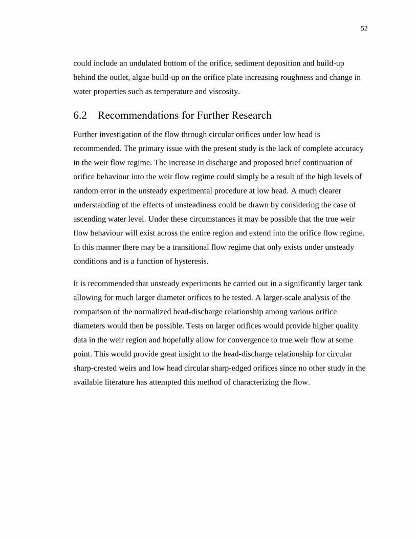
52

could include an undulated bottom of the orifice, sediment deposition and build-up

behind the outlet, algae build-up on the orifice plate increasing roughness and change in

water properties such as temperature and viscosity.

6.2 Recommendations for Further Research

Further investigation of the flow through circular orifices under low head is

recommended. The primary issue with the present study is the lack of complete accuracy

in the weir flow regime. The increase in discharge and proposed brief continuation of

orifice behaviour into the weir flow regime could simply be a result of the high levels of

random error in the unsteady experimental procedure at low head. A much clearer

understanding of the effects of unsteadiness could be drawn by considering the case of

ascending water level. Under these circumstances it may be possible that the true weir

flow behaviour will exist across the entire region and extend into the orifice flow regime.

In this manner there may be a transitional flow regime that only exists under unsteady

conditions and is a function of hysteresis.

It is recommended that unsteady experiments be carried out in a significantly larger tank

allowing for much larger diameter orifices to be tested. A larger-scale analysis of the

comparison of the normalized head-discharge relationship among various orifice

diameters would then be possible. Tests on larger orifices would provide higher quality

data in the weir region and hopefully allow for convergence to true weir flow at some

point. This would provide great insight to the head-discharge relationship for circular

sharp-crested weirs and low head circular sharp-edged orifices since no other study in the

available literature has attempted this method of characterizing the flow.

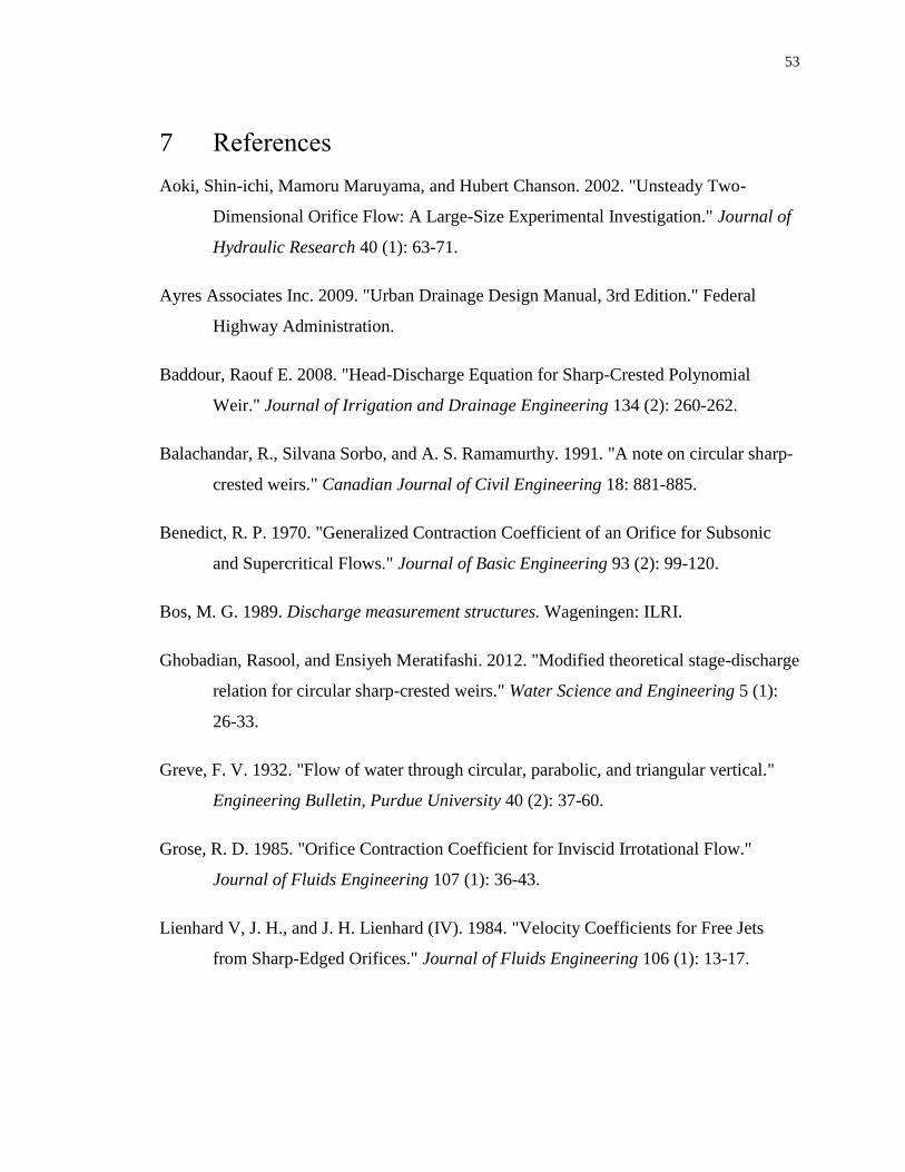
53

7 References

Aoki, Shin-ichi, Mamoru Maruyama, and Hubert Chanson. 2002. "Unsteady Two-

Dimensional Orifice Flow: A Large-Size Experimental Investigation." Journal of

Hydraulic Research 40 (1): 63-71.

Ayres Associates Inc. 2009. "Urban Drainage Design Manual, 3rd Edition." Federal

Highway Administration.

Baddour, Raouf E. 2008. "Head-Discharge Equation for Sharp-Crested Polynomial

Weir." Journal of Irrigation and Drainage Engineering 134 (2): 260-262.

Balachandar, R., Silvana Sorbo, and A. S. Ramamurthy. 1991. "A note on circular sharp-

crested weirs." Canadian Journal of Civil Engineering 18: 881-885.

Benedict, R. P. 1970. "Generalized Contraction Coefficient of an Orifice for Subsonic

and Supercritical Flows." Journal of Basic Engineering 93 (2): 99-120.

Bos, M. G. 1989. Discharge measurement structures. Wageningen: ILRI.

Ghobadian, Rasool, and Ensiyeh Meratifashi. 2012. "Modified theoretical stage-discharge

relation for circular sharp-crested weirs." Water Science and Engineering 5 (1):

26-33.

Greve, F. V. 1932. "Flow of water through circular, parabolic, and triangular vertical."

Engineering Bulletin, Purdue University 40 (2): 37-60.

Grose, R. D. 1985. "Orifice Contraction Coefficient for Inviscid Irrotational Flow."

Journal of Fluids Engineering 107 (1): 36-43.

Lienhard V, J. H., and J. H. Lienhard (IV). 1984. "Velocity Coefficients for Free Jets

from Sharp-Edged Orifices." Journal of Fluids Engineering 106 (1): 13-17.

54

Ontario Ministry of Environment. 2003. "Stormwater Management Planning and Design

Manual."

Prohaska II, Paul David. 2008. "Investigation of the Discharge Coefficient for Circular

Orifices in Riser Pipes." Master's Thesis.

Smith, D., and W. J. Walker. 1923. "Orifice Flow." Proceedings of the Institution of

Mechanical Engineers. 23-26.

Staus, A. 1931. "Der beiwert kreisrunder uberfalle." Wasserkraft und Wasserwirtschaft

25 (11): 122-123.

Stevens, J. C. 1957. "Flow through Circular Weirs." Journal of the Hydraulics Division

83 (6).

n.d. Stormwater Management Fact Sheet: Stormwater Wetland. Accessed Aug 29, 2013.

http://www.stormwatercenter.net/.

Toronto and Region Conservation Authority. 2009. "Preparing for the Impacts of Climate

Change on Stormwater and Floodplain Management: A Review of Adaptation

Plans and Practices."

Tullis, B. P., E. C. Olsen, and K. Garadner. 2008. "Reducing Detention Volumes with

Improved Outlet Structure." Journal of Irrigation and Drainage Engineering 134

(6): 824-830.

Vatankhah, Ali R. 2010. "Flow measurement using circular sharp-crested weirs." Flow

Measurement and Instrumentation 21: 118-122.

55

Appendices

Appendix A: Circular Weir Discharge Coefficients by Bos (1989)

Table A-1: Circular weir discharge coefficients for various head levels, after Bos (1989)

𝑯 𝑫⁄ 𝑪𝒆 𝑯 𝑫⁄ 𝑪𝒆

0 - 0.55 0.593

0.05 0.75 0.60 0.594

0.1 0.65 0.65 0.595

0.15 0.623 0.70 0.596

0.2 0.610 0.75 0.597

0.25 0.604 0.80 0.599

0.3 0.600 0.85 0.600

0.35 0.597 0.90 0.602

0.40 0.595 0.95 0.604

0.45 0.594 1.0 0.606

0.50 0.593

56

Appendix B: Dimensional Analysis of Weir/Orifice Flow

The first step in any dimensional analysis is to select the independent variables. The

discharge through a circular orifice or weir is a function of the orifice diameter D and the

upstream head H, driven by the effects of gravity g as follows

𝑄 = 𝑓(𝐻, 𝐷, 𝑔) [B-1]

The density and viscosity would also be relevant parameters but no such viscous or

compressibility effects are considered as part of this study. Since there are only two

dimensions present (length and time) there will only be one (𝑁 = 𝑛 − 𝑚 = 3 − 2 = 1) PI

group

Π𝑄 = 𝑓(Π1) [B-2]

By inspection the first PI group will be

Π1 =𝐻

𝐷 [B-3]

The discharge PI group will be

Π𝑄 =𝑄

𝐷2.5𝑔0.5 [B-4]

Note that the upstream head H could be used interchangeably with the diameter in Eq.

[B-4]. Subbing these results back into Eq. [B-2] yields

𝑄

𝐷2.5𝑔0.5 = 𝑓 (𝐻

𝐷) [B-5]

This relationship is readily developed from the standard orifice equation in the following

steps starting with Eq. [2-10]

𝑄𝑎 = 𝐶𝑒𝐴0√2𝑔𝐻 [2-10]

57

Considering the cross-sectional area for a circular orifice and rearranging

𝑄𝑎

𝐷2√𝑔= 𝜋𝐶𝑒√2𝐻 [B-6]

If we then divide both sides of the equation by √𝐷 we obtain

𝑄𝑎

𝐷2.5√𝑔= 𝜋√2𝐶𝑒√

𝐻

𝐷 [B-7]

Equation [B-7] is equivalent to Eq. [2-10] in all respects, and can be effectively used to

compare the flow between orifices of different diameter. For circular weir flow and

theoretical orifice flow the function applied to the normalized head will be different. The

power which is applied to the normalized head will not be a constant value as it is with

the standard orifice equation. This is discussed further in Section 5.2 where the

theoretical and experimental powers are compared to establish the presence of true orifice

and weir flow.

58

Appendix C: Non-Steady Experimental Calibration Data

Table C-1: Calibration data for 3cm diameter orifice experiments

Voltage Readings (V)

Test # 1 2 3 4 5

Head(cm)

0 1.112 1.11 1.11 1.11 1.111

18.8

33.8

48.8

58.8 1.671 1.669 1.669 1.67 1.671

68.8 1.765 1.764

78.8 1.86 1.858 1.859 1.859 1.86

88.8 1.954 1.953

98.8 2.048 2.047 2.047 2.048 2.049

Head (cm)

0 20 40 60 80 100 120

Vo

ltag

e (

V)

1.0

1.2

1.4

1.6

1.8

2.0

2.2

1

2

3

4

5

Figure C-1: Sample plotted calibration data for 3cm diameter orifice experiments

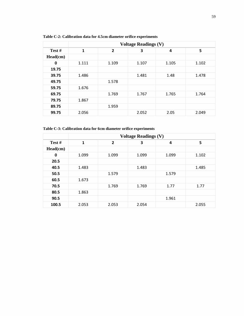
59

Table C-2: Calibration data for 4.5cm diameter orifice experiments


Test # 1 2 3 4 5

Head(cm)

0 1.111 1.109 1.107 1.105 1.102

19.75

39.75 1.486 1.481 1.48 1.478

49.75 1.578

59.75 1.676

69.75 1.769 1.767 1.765 1.764

79.75 1.867

89.75 1.959

99.75 2.056 2.052 2.05 2.049

Table C-3: Calibration data for 6cm diameter orifice experiments


Test # 1 2 3 4 5

Head(cm)

0 1.099 1.099 1.099 1.099 1.102

20.5

40.5 1.483 1.483 1.485

50.5 1.579 1.579

60.5 1.673

70.5 1.769 1.769 1.77 1.77

80.5 1.863

90.5 1.961

100.5 2.053 2.053 2.054 2.055

60

Appendix D: Steady-State Experimental Measurements

Table D-1: Head measurements and discharge results for steady state experiments

Head above

invert(cm)

Calculated Discharge

(m3/s)

Head above

invert(cm)

Calculated Discharge

(m3/s)

2.9 0.000325 9.2 0.00115

2.9 0.000326 9.2 0.001152

2.9 0.000324 9.2 0.001152

3.6 0.000439 9.2 0.001147

3.6 0.00044 10.6 0.001264

3.6 0.000434 10.6 0.001268

3.6 0.000434 10.6 0.00126

3.6 0.00044 10.6 0.001264

4.05 0.000542 13.5 0.001459

4.05 0.000543 13.5 0.001477

4.05 0.000543 13.5 0.001468

4.05 0.000547 13.5 0.001459

4.5 0.000614 13.5 0.001446

4.5 0.000609 16.3 0.001633

4.5 0.000618 16.3 0.001624

4.5 0.000609 16.3 0.001636

4.2 0.00057 16.3 0.001609

4.2 0.000559 16.3 0.001609

4.2 0.000568 19.8 0.001853

4.2 0.000559 19.8 0.001841

4.9 0.000706 19.8 0.001822

4.9 0.00071 19.8 0.001847

4.9 0.000707 19.8 0.001847

4.9 0.000704 24.3 0.002068

4.9 0.000704 24.3 0.002062

5.75 0.000798 24.3 0.002037

5.75 0.000795 24.3 0.002074

5.75 0.000798 24.3 0.002074

5.75 0.000793

7.7 0.001015

7.7 0.001015

7.7 0.001012

7.7 0.001012

61

Appendix E: LOESS Smoothing Technique Details

As discussed in Chapter 5 LOESS smoothing technique was used to combine the data

from all trials for each diameter. It was also used to combine the normalized results of the

3cm and 4.5cm diameter orifices. This technique uses a least squares regression for small

subsets of data in order to predict the local values. A 2nd order polynomial was fit to a

subset of data points surrounding each point being considered. The size of the subset of

data was determined in such a manner as to minimize the standard deviation of the error.

If either too small or too large a number of data points are included in each subset it will

cause increased error, if a 2nd order polynomial fit is maintained. For an example a

summary of the values calculated for the 4.5cm diameter orifice is shown in Table E-1.

The total number of data points in the 4.5cm orifice data set from all 5 trials is 4348.

There is quite obviously a large range of acceptable number of points to include, this

would not always be the case with data that is more irregular with higher error.

Table E-1: RMS of error associated with various data subset sizes

No. of Points Included RMS error

6 3.76*10-6

10 1.11*10-5

50 1.06*10-5

100 9.50*10-6

200 9.41*10-6

400 9.99*10-6

800 1.08*10-6

1500 1.69*10-5

62

Curriculum Vitae

Name: Phil Spencer

Post-secondary Western University

Education and London, Ontario, Canada

Degrees: 2007-2011 B.E.Sc.

Western University

London, Ontario, Canada

2011-Present M.E.Sc.

Honours and QEII Graduate Scholarship in Science & Technology, 2012

Awards: Stantec Consulting Ltd. Civil Engineering Achievement Award, 2010 Vander Laan Undergraduate Scholarship in Engineering, 2009

Lloyd W. Bracewell-Bracewell Engineering Inc. Award, 2009

Related Work Teaching Assistant

Experience Western University

2011-2013

NSERC Undergraduate Student Research Award

Western University

2009

Documents

Investigation of Discharge Behaviour From a Sharp-Edged