A thesis submitted to the

University of Colorado in partial fulfillment

of the requirement for the degree of

Master of Science

Department of Civil, Architectural, and Environmental Engineering

1999

Investigation and Quantification of Boundary Reaction Effect on Solute Transport in a

Circular Pipe Reactor - Application to Laminar and Turbulent Flows

by

STEVEN T. SETZER

B.S., Clarkson University, 1997

This thesis entitled:

Investigation and Quantification of Boundary Reaction Effect on

Solute Transport in a Circular Pipe Reactor - Application to Laminar and

Turbulent Flows

written by Steven T. Setzer

has been approved for the Department of Civil and Environmental

Engineering

Chair of Committee

Committee Member

Date

The final copy of this thesis has been examined by the

signators, and we find that both the content and the form

meet acceptable presentation standards of scholarly work in

the above mentioned discipline.

Setzer, Steven (M.S., Civil Engineering)

Investigation and Quantification of Boundary Reaction Effect on Solute Transport in a

Circular Pipe Reactor - Application to Laminar and Turbulent Flows

Thesis directed by Professor Harihar Rajaram

iii

This thesis examines the effects of a boundary reaction on the effective one-

dimensional transport parameters for a biofilm coated pipe reactor. Both laminar and

turbulent flow conditions are explored. A particle tracking model is used to compute

the effective transport parameters and is verified with analytical results for the laminar

flow case.

After a sufficient development time elapses, the influence of the initial solute

distribution becomes insignificant and the effective decay rate, velocity, and dispersion

coefficients become constants. The laminar flow model shows that a reactive boundary

with first order reaction kinetics leads to first order kinetics in the average, cross-sec-

tional bulk flow concentration. The presence of a reactive boundary causes an increase

in the effective velocity of the solute plume and a decrease in the effective longitudinal

dispersion. It is shown that for laminar flow, the Reynolds number has no impact on

the effective transport parameters. Previous studies that have inferred a correlation

between the effective decay rate and Reynolds number in the laminar flow regime, are

apparently based on the “pre-asymptotic” decay constant and therefore reflect the

effects of entrance gradient development.

A turbulent flow model with no boundary reaction was developed, incorporat-

ing accurate representations of the velocity profile and turbulent diffusivity in the wall

region. The results of this model are compared to Taylor’s classical result of Kau* (K =

10.1 = constant) for the effective longitudinal dispersion coefficient. The model shows

that Taylor’s result does not apply over a wide range of Reynolds numbers and that the

coefficient K in fact varies with Reynolds number. The addition of a boundary reaction

to the turbulent flow model shows that Reynolds number does have an impact on the

effective transport parameters under turbulent conditions. This results from changes in

the laminar sublayer thickness.

Setzer, Steven (M.S., Civil Engineering)

Investigation and Quantification of Boundary Reaction Effect on Solute Trans-

port in a Circular Pipe Reactor - Application to Laminar and Turbulent Flows

Thesis directed by Professor Harihar Rajaram

iv

Acknowledgments

First I’d like to thank Dr. Hari Rajaram for his guidance, advice, and time dur-

ing this research. I truly appreciate the time he took out of his insanely busy schedule

to direct me. I couldn’t have had a better advisor.

Thanks to everyone at CADSWES who gave me their support and had to deal

with all my CPU poaching. Special thanks to Andrew Gilmore, Janet “Frame Queen”

Yowell (who probably deserves some sort of shrine for all the help she gave me), and

Edie Zagona for giving me the time to get this done.

No thanks to all my friends for providing endless distractions and being

directly responsible for the length of time it took to get this done. But on the other

hand, thanks for helping me stay semi-sane during the rough parts.

Finally, thanks to my parents for everything they’ve done for me basically

since birth.

Contents

Introduction . . . . . . . . . . . . . . . . . . . . . . . . . . . . . . . . . . . . . . . . . . . . . . . . . . . . . . . 1

1 Background and Thesis Objectives . . . . . . . . . . . . . . . . . . . . . . . . . . . . . . . . . . . . . 7

Background . . . . . . . . . . . . . . . . . . . . . . . . . . . . . . . . . . . . . . . . . . . . . . . . . . . . . . 7

Mass Balance Equations . . . . . . . . . . . . . . . . . . . . . . . . . . . . . . . . . . . . . . . . 7

Shear Flow Dispersion. . . . . . . . . . . . . . . . . . . . . . . . . . . . . . . . . . . . . . . . . . 8

Taylor Dispersion in Laminar Flow. . . . . . . . . . . . . . . . . . . . . . . . . . . . . . . 10

Taylor Dispersion in Turbulent Flow . . . . . . . . . . . . . . . . . . . . . . . . . . . . . 11

Properties of the Concentration Distribution . . . . . . . . . . . . . . . . . . . . . . . . 14

Effects of a Boundary Reaction . . . . . . . . . . . . . . . . . . . . . . . . . . . . . . . . . . 17

Summary of Previous Work on Two-Region Systems with a Boundary Reaction . . . . . . . . . . . . . . . . . . . . . . . . . . . . . . . . . . . . . . . . . . . . . . . 20

Experiments by Horn and Hempel. . . . . . . . . . . . . . . . . . . . . . . . . . . . . . . . 20

Modeling Oxygen Consumption by Biofilms in Open Channel Flow . . . . 24

Method of Moments Analysis of Transport with Boundary Reactions . . . . 25

Limitations of Previous Work . . . . . . . . . . . . . . . . . . . . . . . . . . . . . . . . . . . 26

Thesis Objectives . . . . . . . . . . . . . . . . . . . . . . . . . . . . . . . . . . . . . . . . . . . . . . . . 26

Analytical Expressions for One-Dimensional Effective Parameters . . . . . . 27

Development of Particle Tracking Model . . . . . . . . . . . . . . . . . . . . . . . . . . 27

Analysis of Biofilm Characteristics and Diffusive Transport Parameters . . . . . . . . . . . . . . . . . . . . . . . . . . . . . . . . . . . . . . . . . . . . . . . . . . 28

2 Development of Particle Tracking Models. . . . . . . . . . . . . . . . . . . . . . . . . . . . . . . 29

General Particle Tracking Theory: Random Walk Method . . . . . . . . . . . . . . . . 29

Laminar Flow Models . . . . . . . . . . . . . . . . . . . . . . . . . . . . . . . . . . . . . . . . . . . . . 31

Transport Within the Bulk Flow . . . . . . . . . . . . . . . . . . . . . . . . . . . . . . . . . 31

Transport and Decay Within the Biofilm. . . . . . . . . . . . . . . . . . . . . . . . . . . 33

Bulk Flow - Biofilm Interface Condition. . . . . . . . . . . . . . . . . . . . . . . . . . . 35

Timestep Restrictions. . . . . . . . . . . . . . . . . . . . . . . . . . . . . . . . . . . . . . . . . . 37

Turbulent Flow Models. . . . . . . . . . . . . . . . . . . . . . . . . . . . . . . . . . . . . . . . . . . . 39

v

Mass Transport in the Vicinity of the Pipe Wall . . . . . . . . . . . . . . . . . . . . . 39

Mass Transport in the Turbulent Core . . . . . . . . . . . . . . . . . . . . . . . . . . . . . 42

Velocity and Diffusivity Profiles . . . . . . . . . . . . . . . . . . . . . . . . . . . . . . . . . 43

Bulk Flow Transport Step Equations. . . . . . . . . . . . . . . . . . . . . . . . . . . . . . 46

Timestep Restrictions. . . . . . . . . . . . . . . . . . . . . . . . . . . . . . . . . . . . . . . . . . 47

System Characterization . . . . . . . . . . . . . . . . . . . . . . . . . . . . . . . . . . . . . . . . . . . 48

3 Analytical Solution to Transport in Laminar and Turbulent Flow. . . . . . . . . . . . . 50

Laminar Flow Solutions . . . . . . . . . . . . . . . . . . . . . . . . . . . . . . . . . . . . . . . . . . . 50

Solution for the Effective Decay Constant . . . . . . . . . . . . . . . . . . . . . . . . . 51

Solution for Effective Velocity . . . . . . . . . . . . . . . . . . . . . . . . . . . . . . . . . . 55

Solution for the Effective Dispersion Coefficient . . . . . . . . . . . . . . . . . . . . 56

Turbulent Flow Solution . . . . . . . . . . . . . . . . . . . . . . . . . . . . . . . . . . . . . . . . . . . 57

4 Particle Tracking Results and Verification. . . . . . . . . . . . . . . . . . . . . . . . . . . . . . . 59

Laminar Flow Results . . . . . . . . . . . . . . . . . . . . . . . . . . . . . . . . . . . . . . . . . . . . . 60

Numerical Issues . . . . . . . . . . . . . . . . . . . . . . . . . . . . . . . . . . . . . . . . . . . . . 64

Dependence of Transport Parameters on Reynolds Number. . . . . . . . . . . . 68

Sensitivity to Porosity and Dbio/D . . . . . . . . . . . . . . . . . . . . . . . . . . . . . . . 69

Diffusion Limited Versus Rate Limited Systems . . . . . . . . . . . . . . . . . . . . 73

Effects of Diffusion Limitation . . . . . . . . . . . . . . . . . . . . . . . . . . . . . . . . . . 75

Turbulent Flow Results for a Smooth Pipe . . . . . . . . . . . . . . . . . . . . . . . . . . . . . 78

Turbulent Transport With No Boundary Reaction . . . . . . . . . . . . . . . . . . . 78

Turbulent Transport with a Reactive Biofilm . . . . . . . . . . . . . . . . . . . . . . . 80

Reynolds Number Dependence . . . . . . . . . . . . . . . . . . . . . . . . . . . . . . . . . . 82

Sensitivity to Damkohler Number . . . . . . . . . . . . . . . . . . . . . . . . . . . . . . . . 85

5 Conclusion . . . . . . . . . . . . . . . . . . . . . . . . . . . . . . . . . . . . . . . . . . . . . . . . . . . . . . . 88

References. . . . . . . . . . . . . . . . . . . . . . . . . . . . . . . . . . . . . . . . . . . . . . . . . . . . . . . . . . 91

vi

vii

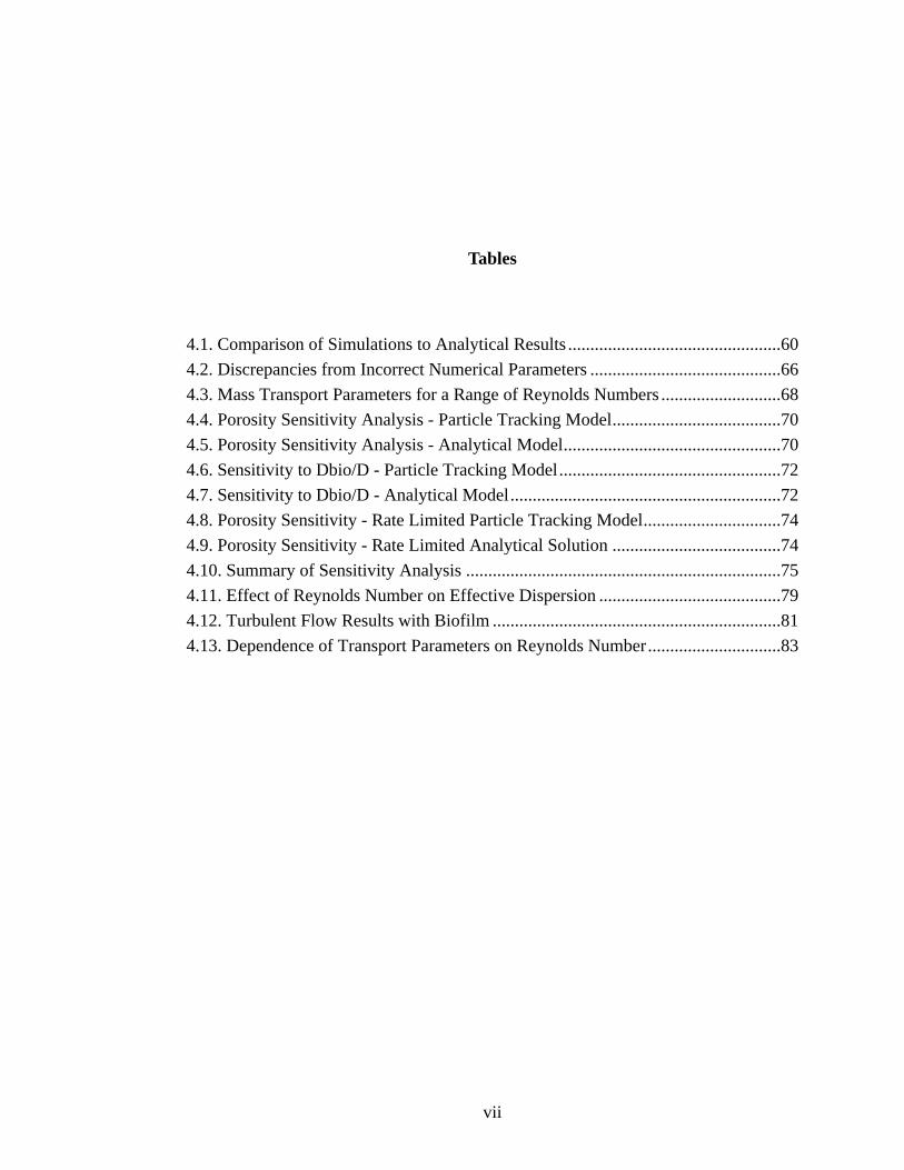
Tables

4.1. Comparison of Simulations to Analytical Results ................................................60

4.2. Discrepancies from Incorrect Numerical Parameters ...........................................66

4.3. Mass Transport Parameters for a Range of Reynolds Numbers ...........................68

4.4. Porosity Sensitivity Analysis - Particle Tracking Model......................................70

4.5. Porosity Sensitivity Analysis - Analytical Model.................................................70

4.6. Sensitivity to Dbio/D - Particle Tracking Model..................................................72

4.7. Sensitivity to Dbio/D - Analytical Model.............................................................72

4.8. Porosity Sensitivity - Rate Limited Particle Tracking Model...............................74

4.9. Porosity Sensitivity - Rate Limited Analytical Solution ......................................74

4.10. Summary of Sensitivity Analysis .......................................................................75

4.11. Effect of Reynolds Number on Effective Dispersion .........................................79

4.12. Turbulent Flow Results with Biofilm .................................................................81

4.13. Dependence of Transport Parameters on Reynolds Number..............................83

viii

Figures

1.1. Radial Control Volume...........................................................................................8

1.2. Horn and Hempel Results .....................................................................................22

1.3. Entrance Length Region .......................................................................................23

2.1. Dimensionless Velocity Distribution (Wall to Pipe Axis)....................................44

2.2. Dimensionless Velocity Distribution (Wall Region - Turbulent Core) ................44

2.3. Diffusivity/Viscosity Distribution (Wall to Pipe Axis) ........................................45

2.4. Eddy Diffusivity in Wall Region ..........................................................................45

2.5. Diffusivity/Viscosity Distribution (Wall Region - Turbulent Core).....................46

4.1. Zeroth Moment Curve...........................................................................................62

4.2. First Moment Curve..............................................................................................63

4.3. Second Moment Curve .........................................................................................64

4.4. Zeroth Moment - Too Few Particles.....................................................................65

4.5. Second Moment - Too Few Particles....................................................................65

4.6. Zeroth Moment - Large Dt....................................................................................67

4.7. Second Moment - Large Dt...................................................................................68

4.8. Effective Decay vs. Da .........................................................................................76

4.9. Effective Velocity vs. Da......................................................................................77

4.10. Effective Dispersion vs. Da ................................................................................78

4.11. Effect of Reynolds Number on Effective Decay ................................................84

4.12. Effect of Reynolds Number on Effective Dispersion .........................................84

4.13. Effective Decay vs. Damkohler Number ............................................................85

4.14. Effective Dispersion vs. Damkohler Number.....................................................87

Introduction

Solute transport and reactions are becoming increasingly important topics in

the field of Water Resources and Environmental Engineering. In recent years, more

emphasis is being placed on water quality than water quantity. In both surface water

and groundwater, it is essential to understand the fate and transport of contaminants in

natural waters in order to effectively manage water quality. Contaminant transport is a

influenced by hydrodynamics as well as the chemistry and biology of the aquatic sys-

tem. This research will focus on describing the hydrodynamics of transport in the pres-

ence of a biological reaction.

Transport within a moving fluid is a result of two processes: advection and dif-

fusion. Advection is solute transport that results from the mean motion of a fluid while

diffusion is transport that results from the random motion of the solute molecules.

Using a control volume and balancing mass, a partial differential equation can be

derived to describe solute transport in a three dimensional system. This equation is the

widely known advection-diffusion equation. A reaction term can be added to accom-

modate a chemical or biological reaction.

The advection-diffusion equation can be modified to describe mass transport in

almost any physical system. However for the large-scale, multi-dimensional systems

usually studied in engineering applications, the solution of this equation can become

very complicated or even impossible. Simplifying assumptions are invariably required

to reduce the complexity of the solution. One approach is to reduce the dimensionality

of the equations and describe the system in terms of “effective” parameters. The effec-

tive parameters serve to capture the effects of multiple dimensions so a system can be

described in a single dimension. The goal of this thesis is to quantify the effective

transport parameters for a circular pipe, with and without a reactive biofilm, under

laminar and turbulent flow conditions.

The three dimensional advection-diffusion equation for concentration in a cir-

cular pipe with a boundary reaction can be reduced to one dimension (along the axis of

the pipe) in terms of the cross-sectional concentration. The solution of this equation

involves an effective decay constant, an effective velocity, and an effective dispersion

coefficient (termed the effective transport parameters). When describing the system in

multiple dimensions, the decay constant used in the advection-diffusion equation

would be the decay constant in the reactive biofilm. Solute would decay according to

this decay constant only when it is located in the biofilm region of the pipe. However,

the effective decay rate used to describe the system with one dimension, represents the

overall reduction of the cross sectional average concentration due to the presence of a

boundary reaction. It is thus likely to be much smaller than the decay rate within the

biofilm, and should also reflect the influence of diffusive exchange between the bulk

flow and biofilm. The effective velocity represents the longitudinal (axial) velocity of

the center of mass of the solute plume and the effective dispersion coefficient repre-

sents the spread of the solute plume in the longitudinal direction.

Horn and Hempel (1995) attempted to quantify the effective decay coefficient

for a short tube reactor under laminar flow conditions. The study used a numerical

model, calibrated with experimental data, to quantify the effects of a reactive biofilm

on bulk flow mass transfer. The goal of the study was to modify an existing mass trans-

fer equation, for a pipe with no biofilm, to include the effects of a boundary reaction.

2

While the mass transfer coefficient empirically developed by Horn and Hempel

matched their experimental data quite well, it appears that their interpretation of the

mechanisms controlling mass transfer and reaction is incorrect. In particular, they pro-

pose a Reynolds number dependence of the effective decay rate, even though all their

experiments were carried out in the laminar flow regime. We believe that the empirical

relationships developed by Horn and Hempel are reactor-specific, in other words, they

can only model the mass transfer coefficient for their reactor and are not generalizable

to all coated biofilm pipe reactors. Due to the short length of their pipe reactor, it

appears that their results reflect the influence of laminar flow that is not yet fully devel-

oped (for the higher flow rate cases) and “pre-asymptotic transport”, wherein the diffu-

sive interactions between the pipe and biofilm have not reached an equilibrium

condition. Cox (1997) showed that under these conditions, representation of one-

dimensional transport in terms of an effective decay constant or mass transfer coeffi-

cient is not valid. In fact, for fully developed laminar flow, after diffusive equilibrium

between the biofilm and bulk flow is achieved, Cox (1997) showed that the effective

decay constant is independent of Reynolds number.

Cox (1997) used a method of moments approach to analytically solve the one-

dimensional advection-diffusion equation for a circular pipe with a reactive boundary

under laminar flow conditions. This resulted in analytical expressions for the effective

decay, effective velocity, and effective dispersion coefficient. The results were verified

with a finite difference numerical solution of the multi-dimensional advection-diffu-

sion equation. The analytical expressions were successful in demonstrating the effects

of a reactive biofilm on the effective transport coefficients. However the models were

limited to laminar flow conditions and were subject to inaccuracies under certain con-

ditions. Also, the numerical model was subject to considerable numerical dispersion.

The research performed in this thesis aims to reproduce Cox’s results with a more

accurate and flexible modeling approach and to extend these models to include turbu-

3

lent flow conditions.

A particle tracking model was constructed to simulate mass transport in a cir-

cular pipe. The theory behind particle tracking models involves statistics and the ran-

dom walk method of modeling. Basically the model uses a large number of particles

which move independently of one another. Each particle is subject to random motion

but is restricted so that the average motion of all the particles meets certain statistical

requirements. The idea is that each particle represents a solute molecule that moves

about due to Brownian motion. Depending on the location of the particle in the sys-

tem, it may also be subject to advection due to a velocity field or large scale random

motion caused by turbulence. The velocity field, degree of random particle motion,

and statistical nature of the model can be adjusted to accommodate various physical

systems.

Since particle tracking models are based on statistics and do not involve a solu-

tion to the advection-diffusion equation, they can be used to describe highly complex

physical systems that could not be modelled otherwise. The application of particle

tracking models to the field of groundwater hydrology is highly relevant. They are cur-

rently used to describe contaminant transport in porous media and fractured flow sys-

tems. However, the particle tracking model developed in this research is designed to

specifically describe solute transport in a circular pipe. The laminar flow results

obtained from the particle tracking model coincide with Cox’s research and give valu-

able insight to the relationship between biofilm characteristics and the effective trans-

port parameters. The zeroth, first and second mass moments of the solute plume are

used to determine the transport parameters. In general, as the reactive properties of the

biofilm increase, the effective decay rate increases and the effective dispersion

decreases.

There are two important aspects to the development of the turbulent flow

model. The first deals with the velocity and diffusivity profiles used in the model. (In

4

turbulent flow radial transport occurs as a result of turbulent eddies as opposed to

molecular diffusion. The term used to describe this form of radial transport is the eddy

diffusivity and it varies with the radial location in the pipe.) A pipe experiencing turbu-

lent flow conditions is comprised of two distinct regions of flow; the turbulent core and

the laminar boundary layer. The turbulent core makes up the majority of the pipe cross

section and is characterized by large rotational eddies and high flow velocities. The

laminar boundary layer exists very close to the pipe wall. In this region the turbulent

eddies dissipate and viscous forces tend to dominate the flow field much like laminar

flow. The velocity and diffusivity profiles in the turbulent core are well defined and

have been confirmed by experimentation; however in the wall region this is not the

case. There have been several attempts to develop velocity and diffusivity profiles for

the laminar sublayer that are continuous with the respective profiles in the turbulent

core. While there is some debate about the exact nature of the wall region, one of the

more well known studies was used to develop the velocity and diffusivity profiles in

this research.

While there has been considerable research in describing the wall region of a

pipe in turbulent flow, no attempt has been made at describing the nature of transport

in the entire system since Taylor’s classical work (Taylor, 1954). Taylor attempted to

quantify the effective dispersion coefficient in a circular pipe under turbulent flow con-

ditions. At that time, the universal velocity profile for the turbulent core had not been

developed and no extensive research had been performed on the velocity and diffusiv-

ity in the wall region. For the turbulent core, a velocity profile which was very near to

the universal profile was used. A linear velocity profile was used in the wall region.

Given these profiles, Taylor showed that the effective dispersion coefficient can be

expressed as 10.1au* where a is the pipe radius and u* is the shear velocity. The mod-

els developed in this research using the more recent expressions for velocity in the

wall region show that the effective dispersion coefficient varies with Reynolds number

5

and hence the “constant” 10.1 is not really constant. This is an important discovery

since Taylor’s result has been accepted since 1954 and additional research on the topic

has not been performed since then.

The second aspect of the turbulent flow models involves the addition of a reac-

tive biofilm. There is no documentation of any research attempting to describe this

system. The model results show that a reactive biofilm has similar effects on the effec-

tive transport coefficients in a turbulent system as that in a laminar flow system. One

important difference, however, is that in laminar flow the effective decay constant does

not vary with Reynolds number while in turbulent flow it does.

In summary, the particle tracking models developed in this research success-

fully quantify the effective transport parameters for a circular pipe with a boundary

reaction for both laminar and turbulent flow. The laminar flow models produce results

that match with Cox’s analytical and numerical results. The non-reactive turbulent

flow models show that for the more recent velocity profiles in the turbulent core and

the wall region, the effective dispersion coefficient varies with Reynolds number and is

therefore inconsistent with Taylor’s result. This calls for additional physical experi-

mentation of dispersion in turbulent pipe flow for a wide range of Reynolds numbers.

6

Chapter 1

Background and Thesis Objectives

1.1 Background

Mass Balance Equations

Transport within a moving fluid essentially takes place as a result of two mech-

anisms; advection and diffusion. Advection is defined as the transport of solute due to

the mean motion of the fluid. Diffusion, on the other hand, is transport due to the ran-

dom motion (brownian motion) of solute molecules. Using a control volume approach

and performing a mass balance, the following equation can be derived to describe the

advection-diffusion system:

Eq. 1.1

where x is the longitudinal direction, y and z are perpendicular to the longitudinal

direction, t is time, u(y,z) is the velocity in the x direction as a function of y and z, n is

the porosity of the medium, and Dx, Dy, and Dz are the diffusion coefficients in the

respective directions. Equation 1.1 is commonly referred to as the “advection-diffusion

equation.”

Due to radial symmetry, flow within a circular pipe can be described with only

two space variables using a radial coordinate system. In radial coordinates, Equation

nC∂t∂

------- nu y z,( ) C∂x∂

-------x∂

∂ nDxC∂x∂

-------

y∂∂ nDy

C∂y∂

-------

z∂∂ nDz

C∂z∂

------- –––+ 0=

1.1 reduces to:

Eq. 1.2

where r is the radial position. Figure 1.1 illustrates the control volume for the radial

coordinate system.

Figure 1.1: Radial Control Volume

Equation 1.2 can be solved analytically or numerically to determine the con-

centration as a function of time, the radial position, and longitudinal position. This

solution is not easily obtained and is sometimes unnecessary. A more useful approach

would be to develop an equivalent one-dimensional “effective transport” equation.

Shear Flow Dispersion

Shear flows involve velocity distributions perpendicular to the flow direction.

Often, these velocity distributions do not change along the flow direction. An example

of such flow is laminar flow in a straight, closed conduit with a constant cross section.

Common to all shear flows is that solute spreading in the direction of flow is domi-

nated by the velocity profile in the cross section (Fischer, 1979). For example, if a par-

nC∂t∂

------- nu r( ) C∂x∂

------- 1r---

r∂∂ nrDr

C∂r∂

-------

x∂∂ nDx

C∂x∂

------- ––+ 0=

8

ticle was located near the wall of a pipe and another was located in the center of the

pipe, their rate of spreading (with respect to each other) due to velocity differences

would greatly exceed that of molecular diffusion. However, given enough time, a sol-

ute particle’s random motion, due to molecular diffusion, will cause it to sample the

entire velocity profile. Therefore, eventually, the time-averaged velocity of any particle

will equal the cross sectionally averaged velocity in the pipe (Taylor, 1953). However,

the rate of separation of particles will still be much greater than if all particles were

travelling at the same advective velocity. This enhanced spreading due to the interac-

tion between the velocity profile and transverse diffusion is commonly referred to as

dispersion.

Taylor (1953) showed that an effective longitudinal dispersion coefficient can

be used to represent the dispersive effects of both transverse diffusion and the variation

of the velocity profile. This assumption has been shown to be valid only after a “devel-

opment length” or “development time”, whereby the effective longitudinal coefficient

has reached an asymptotic value (Taylor, 1953). Using this assumption, and averaging

the concentration and velocity of the entire cross section, a one dimensional, effective

advection-dispersion equation can be derived:

Eq. 1.3

where C is the cross-section average concentration, u is the average velocity, and D* is

the effective longitudinal dispersion coefficient.

While Equation 1.3 is useful for describing the effective one-dimensional

parameters of a system, it is not always applicable. Initially, the distribution of solute

has a major impact on local concentrations and dispersion. Advective dispersion and

molecular diffusion have yet to reach a balance so an effective dispersion coefficient

cannot be used. In order to model this process, it is necessary to use Equation 1.2.

t∂∂ C u

x∂∂ C D

*

x2

2

∂∂ C–+ 0=

9

After a long enough development time however, each solute particle has sam-

pled the entire velocity field several times and the initial distribution of solute ceases to

have an impact on dispersion. The velocity of each solute particle is independent of its

initial velocity. Advective and diffusive transport have reach an equilibrium and the

effective dispersion coefficient has reached an asymptotic value. Also, the solute con-

centration is uniformly distributed across any given cross section. At this point, a

pseudo-steady state condition has been established in a coordinate system moving at u

and Equation 1.3 can be used to model the process.

Taylor Dispersion in Laminar Flow

At low Reynolds numbers, when viscous forces dominate inertial forces, flow

is laminar. The velocity at any given radial location is constant and the instantaneous

velocity profile is smooth because there are no temporal velocity fluctuations due to

turbulence. Therefore, lateral transport of solute occurs by molecular diffusion only.

As the solute moves through various velocity streamlines, it is transported in the longi-

tudinal direction by advection. Since, at any given time, solute exists throughout the

velocity field, solute separation will occur due to velocity differences (as discussed

above). Molecular diffusion also occurs in the longitudinal direction; however, it is

almost negligible when compared to solute separation and transport by advection. In a

circular pipe, the velocity profile for laminar flow can be described by the familiar par-

abolic profile:

Eq. 1.4

where u(r) is the velocity at radial position, r, umax is the maximum velocity (at the

center of the pipe), and a is the radius of the pipe. If Equation 1.4 is integrated over the

radius of the pipe and divided by the cross sectional area of the pipe, the mean velocity

u r( ) umax 1 r2

a2

-----–

⋅=

10

is calculate as one half of the centerline velocity. Taylor (1953) derived an analytical

expression for the asymptotic value of the effective longitudinal dispersion coefficient

in laminar flow:

Eq. 1.5

or

Eq. 1.6

where D* is the effective longitudinal dispersion coefficient and u is the average cross

sectional velocity. The previous two equations have been verified through laboratory

experimentation and will be used to confirm the models developed in this thesis.

Taylor Dispersion in Turbulent Flow

In turbulent flow, inertial forces dominate viscous forces. The instantaneous

velocity profile is not a smooth curve and the velocity at a given radial position fluctu-

ates with time. Statistical analysis can be used to determined a time-averaged velocity

profile. This is the mean value of the velocity over a time scale which is much greater

than the time scale of the individual fluctuations. In the equations and discussion that

follow, the velocities referred to are always the time-averaged velocities.

Extensive experimentation has shown that the turbulent velocity profile is loga-

rithmic in the radial direction except near the walls of the pipe. A velocity profile that

matches the experimental results can be derive using the Prandlt mixing length theory

(Wilkes, 1999). Assume now that the variable y is the distance from the pipe wall (y =

a - r). Prandlt’s hypothesis assumes that there is a direct proportionality between the

mixing length, l, and the distance from the wall, y. Also assume a constant shear stress,

D* a

2umax

2

192D-----------------=

D* a

2u

2

48D-----------=

11

, which is equal to its value, , at the wall. This is true only for a small interval near

the pipe wall.

Eq. 1.7

Eq. 1.8

where k is a constant. In actuality, Equation 1.7 and Equation 1.8 are overestimates for

both l and . However, both overestimates tend to cancel each other out and give an

excellent result for the turbulent velocity profile (Wilkes, 1999). Mixing length theory

gives the following relationship:

Eq. 1.9

where u is the time-averaged velocity as a function of y. du/dy is recognized as positive

since the time-averaged velocity increases as the distance from the wall increases.

Using Equation 1.7 and Equation 1.8, Equation 1.9 can be rewritten as:

Eq. 1.10

Equation 1.10 integrates to:

Eq. 1.11

where c is a constant of integration.

Equation 1.11 is used to develop what is known as the universal velocity profile

for turbulent flow in a smooth pipe. It is first useful to define some non-dimensional

τ τw

l ky=

τ τ w=

τ

τ ρ l2 ud

yd------

2=

τw ρk2

y2 ud

yd------

2=

u1k---

τw

ρ----- yln c+=

12

parameters. The term is commonly known as the friction velocity or shear

velocity, u*. Using this definition, a dimensionless variables for y and u can be defined

as:

Eq. 1.12

Eq. 1.13

where υ is the kinematic viscosity. Equation 1.11 can now be rewritten as:

Eq. 1.14

where A is the constant of integration and B is 1/k. Experimentation has shown the

constants to be 5.5 and 2.5, respectively. The final form of the universal velocity pro-

file is shown below:

Eq. 1.15

The universal velocity profile matches experimental results in the turbulent core, how-

ever, it does not hold in the wall region because it gives an ever-increasing negative

velocity and an ever-increasing velocity gradient as y approaches zero. The no-slip

condition for fluids in as pipe requires that velocity is zero when y is zero. There is

more than one way to describe the velocity variations in the wall region. This will be

discussed further during the development of the models used to describe this system.

In turbulent flow in a pipe, relatively large rotational eddies are formed in the

region of high shear near the wall which degenerate into progressively smaller eddies,

dissipating energy into heat by the action of viscosity (Wilkes, 1999). The motion of

τw ρ⁄

y+ yu*

υ--------=

u+ u

u*-----=

u+

A B y+ln+=

u+ 5.5 2.5 y

+ln+=

13

these eddies is responsible for the transfer of solute in the radial direction. The coeffi-

cient of lateral transport must therefore include the effects of eddy diffusivity as well

molecular diffusion in order to accurately describe lateral transport. This coefficient,

termed the eddy molecular diffusivity, simply replaces the molecular diffusion coeffi-

cient in the equations used to describe dispersion in laminar flow. Using Reynold’s

analogy, which assumes that the mixing coefficients for momentum and mass are the

same, the eddy molecular diffusivity can be expressed as:

Eq. 1.16

where m is the rate of radial transfer of matter of concentration C.

The extension of the laminar flow analysis to turbulent flow involves using the

universal velocity profile (instead of the laminar flow profile) and the eddy molecular

diffusivity (instead of the molecular diffusion coefficient). The conclusions reached

about the use of the one dimensional advection-dispersion equation (described previ-

ously) remain unchanged (Fischer, 1979). The only significant difference is that the

eddy molecular diffusivity varies as a function radial position. Therefore, Taylor was

able to derive an expression for the asymptotic value of the effective longitudinal dis-

persion coefficient in turbulent flow:

Eq. 1.17

Properties of the Concentration Distribution

In 1956, Aris developed an alternative method for characterizing effective

transport parameters (Aris, 1956). Commonly referred to as the method of moments,

Aris used various moments of the concentration distribution to determine properties of

the advection-dispersion system. The pth concentration moment is defined by the fol-

ε mC∂ r∂⁄

----------------– τ

ρ u∂r∂

-------------- υ–

τw r a⁄( )

ρ u∂r∂

-------------------------– υ–=–= =

D* 10.1au*=

14

lowing equation:

Eq. 1.18

where x is the longitudinal position and C(x,r,t) is the concentration with respect to

longitudinal position, radial position and time.

Equation 1.18 is used to compute the concentration moment at a given radial

position, r. This is not very useful for determining overall effective parameters. The

concentration moment must be integrated over the entire cross section to include all

radial positions. Equation 1.18 then becomes:

Eq. 1.19

where Mp is the cross sectional average of Cp as a function of time, and a is the radius

of the pipe. It is apparent that the zeroth moment, M0(t), represents the total mass in

the system at any time t:

Eq. 1.20

Therefore, the one dimensional effective decay coefficient, k*, can be expressed as:

Eq. 1.21

This comes from the definition of first order kinetics: . For non-reac-

tive transport as described by Equation 1.1 and Equation 1.2, k* = 0 and M0 is a con-

stant equal to the initial mass introduced to the system.

The first moment, M1, is defined as:

C p xpC x r t, ,( ) xd

-∞

+∞

∫=

M p t( ) 2πr xpC x r t, ,( ) x rdd

-∞

+∞

∫0

a

∫=

M 0 t( ) 2πr C x r t, ,( ) x rdd

-∞

+∞

∫0

a

∫=

k* M 0d td⁄

M 0-------------------=

Md td⁄ k*M 0=

15

Eq. 1.22

The first moment represents a weighted summation of longitudinal positions over the

entire system volume. If this weighted sum is divided by the entire mass in the system,

the result is a weighted average of longitudinal positions. This is equivalent to the cen-

ter of mass in the system, defined as:

Eq. 1.23

where X(t) is the mass centroid as a function of time. The change in centroid position

with respect to time represents the effective velocity of the center of mass of the solute

plume:

Eq. 1.24

In a pipe with no reaction, Ueff is equal to the mean velocity of the fluid.

The second moment of mass is defined as:

Eq. 1.25

It can be shown that the longitudinal variance of the solute plume is expressed as:

Eq. 1.26

The rate of change of the variance represents the rate of change of the solute spread in

the longitudinal direction. This has been shown to be proportional to the effective one

dimensional dispersion coefficient (Fischer, 1979).

M 1 t( ) 2πr xC x r t, ,( ) x rdd

-∞

+∞

∫0

a

∫=

X t( )M 1

M 0--------=

U eff

M 1 M 0⁄( )d

td---------------------------- Xd

td-------= =

M 2 t( ) 2πr x2C x r t, ,( ) x rdd

-∞

+∞

∫0

a

∫=

σ2 M 2

M 0-------- X

2t( )–=

16

Eq. 1.27

In general, a non-reactive solute plume will have a gaussian distribution once

the initial development time has elapsed. If a coordinate system that moves with the

mean velocity of the flow is adopted, the mean of the solute distribution is zero and the

variance is: . However, as discussed in the following section, this is not

necessarily the case if a boundary reaction exists.

Effects of a Boundary Reaction

In context of biological treatment of wastewater, biofilm reactors with simpli-

fied geometries have been studied. The objective of these studies are to quantify effec-

tive reaction rates and other effective transport parameters. Among the systems

studied, are biofilm coated pipe reactors (Horn and Hempel, 1995) and (Cox, 1997).

Dissolved oxygen and substrates that are biodegradable can be consumed within the

biofilm. This can be modeled by including a reaction term in the two dimensional

equation (Equation 1.2) that is active only for the boundary region.

Eq. 1.28

where i = 1 refers to the bulk flow and i = 2 refers to the biofilm region. In the bulk

flow region, the reaction term, rxn, is equal to zero ant the porosity is one. Two bound-

ary conditions are used to define the system at the bulk flow - biofilm interface: equal

concentration at the interface

Eq. 1.29

and equal flux at the interface

σ2d

td--------- 2D

*=

σ2 2D*t=

nCi∂t∂

-------- nu r( )Ci∂x∂

-------- 1r---

r∂∂ nDri

Ci∂r∂

--------

x∂∂ nDxi

Ci∂x∂

-------- rxn+––+ 0 i, 1 2,= =

C1 C2 at r, interface= =

17

Eq. 1.30

The reaction term, rxn, may be zero order, first order, or non-linear. In this the-

sis, non-linear reactions are not considered. A zero order reaction term has the form

+nk, where n is the porosity and k is the decay constant. A reaction of this type occurs

at a constant rate regardless of the concentration. A first order reaction is represented

by the term +nkC2 where C2 is the solute concentration in the biofilm. This takes the

form of an exponential decay of solute in the reactive region.

In a laminar flow system, transport of solute to the reactive boundary takes

place by diffusion only. Therefore, transport into the biofilm is governed by the molec-

ular diffusion coefficient and the concentration gradient that exists across the biofilm-

bulk flow interface (according to Fick’s Law) (Cox, 1997). Once the solute reaches the

boundary and enters the biofilm, it then decays according to the appropriate reaction

type. Diffusive transport may take place within the biofilm allowing the solute to re-

enter the bulk flow. Advection of solute usually does not occur within the biofilm coat-

ing on the pipe walls and will not be considered in this thesis.

In a turbulent flow system, there are two regions involved with transport in the

radial or transverse directions. Boundary layer theory dictates that a laminar sublayer

exists very close to the pipe wall where viscous forces dominate inertial forces. Turbu-

lent eddies do not exist in the laminar sublayer so diffusion to the biofilm region is

Fickian in nature and therefore controlled by the molecular diffusion coefficient and

the concentration gradient across the sublayer. In the turbulent core, radial transport is

dominated by the turbulent eddies. The eddy diffusivity control transport to the lami-

nar sublayer.

In order to incorporate a reactive biofilm boundary in the one-dimensional

transport equation, an effective decay term can be added.

Dr1

C1∂r∂

--------- nDr2

C2∂r∂

--------- at r = interface,=

18

Eq. 1.31

where Ueff is the effective velocity, D* is the effective dispersion coefficient, and k* is

the effective decay coefficient. The decay term represents the decay of the cross sec-

tional average concentration. The effective decay rate will be smaller than the decay

rate in the biofilm because decay is confined only to the boundary region. The effective

decay term will reflect the balance that is achieved between the diffusive transport

from the bulk flow into the active boundary regions and the concentration decay within

these regions (Cox, 1997). Initially, diffusive processes will dominate as the solute is

transported to the boundary region. However, once the initial boundary gradients have

been established and the conditions for one-dimensional representation have been

achieved, a constant term can be used in the mass balance for the bulk flow. Cox, in

1997, showed that for laminar flow the effective decay term can be limited by either

diffusion or kinetics, depending upon the magnitude of the decay coefficient in the

biofilm in comparison to the molecular diffusion coefficient. In this thesis, the investi-

gation into the nature of the effective decay term will be continued for laminar flow

systems and extended to turbulent flow.

The one dimensional effective velocity, Ueff, and dispersion, D*, coefficients

will be affected by the existence of a boundary reaction. The effective velocity of the

centroid of the solute plume may or may not travel at the mean speed of flow. Also, the

concentration distribution may not be a normal, symmetrical Gaussian curve. The dis-

tribution will still be Gaussian in nature, however, there may be a degree of skewness

and the variance will be different from that of a solute plume with no boundary reac-

tion. The existence of a reactive boundary will cause the cross sectional concentration

distribution to be non-uniform. More solute will exist in the center of the pipe because

solute near the pipe wall is subject to decay. This will cause the effective velocity of

the solute plume to increase because more mass exists in regions of higher velocity.

t∂∂ C U eff x∂

∂ C D*

x2

2

∂∂ C k

*C+–+ 0=

19

For the same reason, the effective dispersion coefficient will decrease because less sol-

ute will exist in the regions of highest shear (near the wall). In other words, more sol-

ute will exist in the center of the pipe where the velocity variations are less severe.

Therefore, there will be decreased longitudinal separation among the solute particles.

When using the one-dimensional transport equation with a boundary reaction these

parameters need to be adjusted accordingly. Methods of characterizing the effective

one-dimensional parameters will be discussed later in this thesis.

1.2 Summary of Previous Work on Two-Region Systems with a Boundary Reac-tion

Following is a summary of the previous work involving the characterization of

bulk flow - biofilm systems. Also, included is some work dealing with open channel

flow with a reactive bed. The problem of describing mass transport in a system with a

reactive boundary has not been extensively studied in the field of water resources engi-

neering. Most of the background theory is taken from mass transport studies in the

field of chemical engineering or analogous theories in heat transport. Therefore, a well

established background to this research does not exist. The following studies are dis-

cussed to provide a frame of reference and to demonstrate how similar research prob-

lems have been approached in the past.

Experiments by Horn and Hempel

Horn and Hempel (1995) performed a series of experiments aimed at evaluat-

ing the mass transfer coefficients at a bulk flow - biofilm interface. This was done by

modifying an existing expression for radial mass transfer in a circular pipe with no

biofilm to reflect the effects of a biofilm coating. A numerical model was used to cal-

culate concentration profiles and was calibrated by adjusting the mass transfer coeffi-

cient to match the measured profiles. In this way, mass transfer coefficients were

estimated for various flow rates within the laminar flow regime.

20

The Sherwood number, Sh, is a dimensionless number used to describe mass

transfer for laminar flow in tube reactors without biofilms:

Eq. 1.32

where Re is the Reynold’s number, Sc is the Schmidt number (momentum transfer /

mass transfer), d is the tube diameter, and L is the tube length. The length of the tube

reactor used in the experiments and in the models was constant at 163 cm. The diame-

ter of the tube was 1.6 cm and the biofilm thickness was 0.035 cm on average. The

numerical model used to estimate mass transfer was based on the following equation:

Eq. 1.33

where CB and CF are the concentrations in the bulk flow and at the biofilm surface,

respectively, and β is the mass transfer coefficient. Mass transfer coefficients were esti-

mated for various flow rates within a range of Reynold’s numbers from 532 - 1894.

The numerical/experimental mass transfer coefficients were about one order of magni-

tude less than those given by Equation 1.32. It was surmised by Horn and Hempel that

this discrepancy was due to the fact that Equation 1.32 did not account for a boundary

reaction and the boundary layer close to the wall. Therefore it was modified in the fol-

lowing manner to better fit the experimental data:

Eq. 1.34

Figure 1.2 shows the experimental results in relation to Equation 1.32 and Equation

1.34.

Sh 2Re1 2⁄

Sc1 2⁄

d L⁄( )1 2⁄=

DC∂r∂

------- β CB CF–( )=

Sh 2Re1 2⁄

Sc1 2⁄

d L⁄( )1 2⁄ 1 0.0021Re+( )=

21

Figure 1.2: Horn and Hempel Results

In Figure 1.2, “equation 1” represents Equation 1.32 and “equation 4” repre-

sents Equation 1.34. It is obvious that Equation 1.34 fits the data much better that

Equation 1.32. However, it also obvious that the mass transfer coefficient varies with

Reynold’s number. According to the theory of Taylor dispersion in laminar flow (dis-

cussed previously), the effective mass transfer coefficient does not depend on Re.

(Incidentally, in turbulent flow, the effective one-dimensional mass transfer coefficient

is dependent on Reynold’s number. As Reynold’s number increases turbulence

increases and the thickness of the laminar sublayer decreases, thereby increasing mass

transfer to the biofilm region. This is discussed in greater detail in later chapters.) The

tube reactor used in the Horn and Hempel experiments was relatively short (163 cm).

At the lowest Reynold’s number used in the experiments (534), the travel time in the

pipe would be about 50 seconds. According to the theory of shear flow dispersion, an

initial development time is required before the effective mass transfer coefficient

reaches a constant, asymptotic value. The following equation can be used for estimat-

ing the initial development length for laminar flow (Cox, 1997):

22

Eq. 1.35

where L is the development length, Re is the Reynold’s number, and Sc is the Schmidt

number. For a Reynold’s number of 534, this results in a development length of 20000

cm and a development time of about 6000 s. Therefore, the development time is never

reached in the Horn and Hempel experiments. The mass transfer coefficient has not

reached an asymptotic value and the assumption of a constant value for the mass trans-

fer coefficient is not valid. Horn and Hempel’s interpretation of their data using a mass

transfer coefficient dependent on Reynolds number is therefore inappropriate. They

are actually fitting the pre-asymptotic behavior of the effective reaction rate using a

Reynolds number dependence.

In addition to the initial development time required to achieve effective one-

dimensional transport, an entrance development length is required before fully laminar

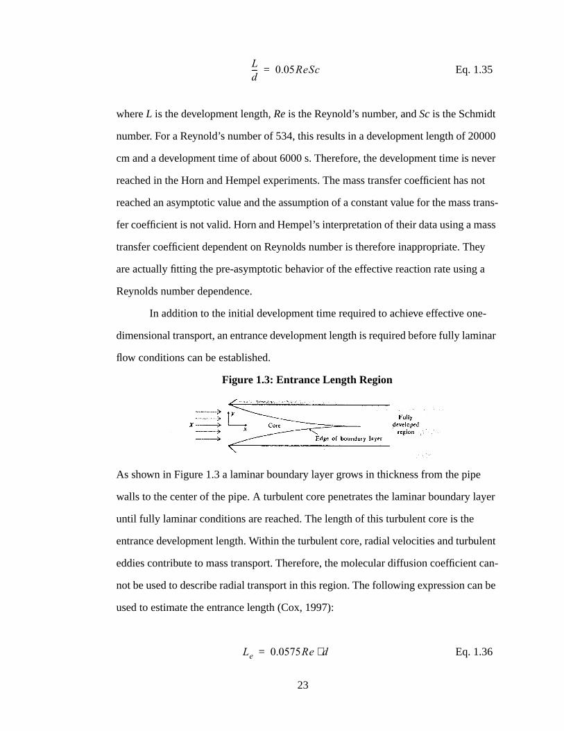
flow conditions can be established.

Figure 1.3: Entrance Length Region

As shown in Figure 1.3 a laminar boundary layer grows in thickness from the pipe

walls to the center of the pipe. A turbulent core penetrates the laminar boundary layer

until fully laminar conditions are reached. The length of this turbulent core is the

entrance development length. Within the turbulent core, radial velocities and turbulent

eddies contribute to mass transport. Therefore, the molecular diffusion coefficient can-

not be used to describe radial transport in this region. The following expression can be

used to estimate the entrance length (Cox, 1997):

Eq. 1.36

Ld--- 0.05ReSc=

Le 0.0575Re d⋅=

23

For the range of Reynold’s numbers used in the Horn and Hempel experiment,

entrance lengths vary from 50 - 100 cm. Therefore, for higher Reynold’s numbers,

fully laminar conditions are not even established within the tube reactor.

It is obvious that the assumption of a constant mass transport coefficient in the

Horn and Hempel tube reactor is invalid. Effective one-dimensional conditions are

never established and in some cases fully laminar conditions are not even established.

Therefore, it is assumed that the mass transfer coefficients calculated by Equation 1.32

and Equation 1.34 represent average transfer coefficients for the length of the reactor.

The values of the coefficients would be dependent upon both the degree of penetration

of the turbulent core and the travel time through the pipe. Thus a direct relationship

between the Reynold’s number and average transfer coefficient would exist. It is

assumed that Equation 1.32 and Equation 1.34 were developed for short tube reactors

with laminar flow, where the reactor lengths are of the same scale as the entrance

lengths. Therefore, their findings are applicable on a reactor specific basis only.

Modeling Oxygen Consumption by Biofilms in Open Channel Flow

In 1994, S. Li and G.H. Chen developed a mathematical model to predict the

removal of dissolved organic substances and the consumption of dissolved oxygen by

attached, benthic biofilms in an open channel flow (Li and Chen, 1994). The conven-

tional Streeter-Phelps equation was combined with the biofilm equations resulting in a

system of equations that could be solved numerically.

The model assumed that transfer of matter occurred from a bulk flow region,

through a diffusion layer (laminar sublayer), and into the biofilm where reaction took

place. Two dimensional mass balance equations were coupled for each of the regions

and included the effects of molecular diffusion through the diffusion layer, mean

velocity in the bulk flow, reaeration in the bulk flow, and Dual Monod reaction kinetics

in the biofilm. The resulting non-linear system was solved by a trial and error approach

24

to a finite difference numerical model.

The results of the model show that the effects of a biofilm have a significant

influence on organic removal and oxygen consumption. The traditional Streeter-Phelps

equation is based on the removal rates of the suspended biomass which are usually

determined from BOD bottle tests. However the modified Streeter-Phelps model

shows that the removal rates caused by the biofilm are greater than those resulting

from suspended biomass. Some studies have shown that streambed biomass accounts

for 90% of the oxygen consumption (Li and Chen, 1994). Li and Chen also studied the

effects of bulk flow velocity on the diffusive layer thickness and benthic uptake. In

general an increase in velocity leads to a decrease in thickness of the diffusive layer.

As diffusive layer thickness decreases, benthic uptake becomes less diffusion limited

so uptake should increase. However, as the bulk flow velocity increases, contact time

with the biofilm decreases and so uptake should decrease. The overall result of the

experiments suggests that contact time is more significant than the diffusive layer

thickness. Another finding made by Li and Chen is that uptake increases as biofilm

thickness increases up to a certain point. Beyond a certain thickness, diffusion limita-

tions dominate and the uptake reaches a constant value. Both the net effects of bulk

flow velocity and biofilm thickness will be explored in this thesis.

Method of Moments Analysis of Transport with Boundary Reactions

Tim Cox (1997) quantified the effects of boundary reactions on bulk flow sol-

ute transport parameters in a biofilm-coated pipe under laminar flow conditions. The

emphasis of the research was to use both numerical and analytical approaches to estab-

lish relationships between effective bulk flow transport parameters and biofilm proper-

ties. Also explored was the time scale associated with the development region of

transport.

Using Aris’ method of moments approach, analytical expressions were devel-

25

oped for the effective one dimensional decay coefficient, the effective velocity, and the

effective dispersion coefficient. These expression will be described in detail in a later

chapter and will be used to verify models developed in this research. The numerical

models were based on a finite-difference approach for solving the advection-disper-

sion equation. These results were used to verify the analytical results. The numerical

model was very successful in verifying the analytical expressions for effective decay

and effective velocity. However there was some discrepancy in the effective dispersion

coefficients. It is believed that this is a result of numerical dispersion commonly

encountered in finite-difference models.

Limitations of Previous Work

Of the previous work just described, only Tim Cox attempted to quantify the

effects of a boundary reaction on the bulk flow transport parameters. However, his

work was limited to laminar flow conditions. Also, the numerical model used in his

research had inaccuracies due to numerical dispersion.

As discussed previously, Horn and Hempel’s experiments were unable to

describe the asymptotic, effective transport parameters. Their work was limited to a

tube reactor that was not long enough to establish conditions that could be described

with one dimensional parameters. Their findings seem to be applicable on a reactor

specific basis only. While Li and Chen were successful in describing a two-region sys-

tem with boundary reactions. Their work was applied to open channel flow and there-

fore, is not directly related to the research in this thesis.

1.3 Thesis Objectives

The background material just described will be used as a basis to characterize

the one-dimensional transport parameters for a laminar and turbulent flow system.

This will first be done for a circular pipe with no biofilm to reproduce the results dis-

cussed previously. Tim Cox, in 1997, extended this theory to a circular pipe with a

26

reactive biofilm under laminar flow conditions. A particle tracking model will be used

to reproduce his results and then extend the analysis further to describe a turbulent

flow system with a reactive biofilm. In this way the problem of numerical dispersion,

as seen in Tim Cox’s work, will be avoided.

The main objective of this work is to show the relationship between various

biofilm characteristics and the effective bulk flow and transport parameters in laminar

and turbulent pipe flow. A particle tracking model is used to simulate 3-dimensional

transport and calculate the resulting effective parameters. These are verified with ana-

lytical results. The particle tracking model is also used to characterize the transport

system in the development stages, before the effective parameters reach an asymptotic

value. The following specific tasks are undertaken to accomplish the stated objectives.

Analytical Expressions for One-Dimensional Effective Parameters

Aris’ method of moments procedure will be applied to a circular pipe with a

reactive biofilm. Only a first order reaction rate will be considered in the derivation of

the analytical expressions. Analytical expressions will be developed for the effective

one-dimensional decay rate, velocity, and dispersion coefficient. These will be used to

verify the particle tracking results and provide insight into the development time of the

system.

Development of Particle Tracking Model

A particle tracking model will be used to simulate 3-dimensional transport in a

circular pipe. Models will be constructed for both laminar and turbulent flow condi-

tions with and without a reactive biofilm. The method of moments will be used to

determine the effective one-dimensional transport parameters. For the case of no

boundary reaction, the model results will be compared to the expressions developed by

Taylor for the effective dispersion coefficient. For the case of a boundary reaction in

laminar flow, the model results will be compared to the analytical expressions derived

27

for a first order boundary reaction. The development of the turbulent flow model will

involve research into the nature of mass transport in the laminar sublayer of the flow

field. Using a velocity profile developed by Wasan and Wilke (1963) and the universal

velocity profile for the turbulent core, the nature of the effective dispersion coefficient

is examined (without the effects of a biofilm) and compared to Taylor’s result of

10.1au*. Finally, the model will be used to characterize the effective transport parame-

ters for a turbulent flow system with a boundary reaction. No previous work was found

on this topic so the model results cannot be verified with accepted results.

Analysis of Biofilm Characteristics and Diffusive Transport Parameters

The models discussed previously will be used to analyze the relationships

between various biofilm characteristics and the effective transport parameters. Specifi-

cally the relationship between diffusion and reaction kinetics. A diffusion limited sys-

tem is one in which the overall effective reaction term is dictated by the rate of

transport into the biofilm. A non-diffusion or reaction rate limited system is one in

which the effective reaction term is governed by the rate of decay within the biofilm.

The nature of the effective transport parameters for both diffusion and reaction limited

systems will be investigated. Also of interest is the nature of solute transport before the

initial development time has elapsed. The effect of biofilm and pipe flow characteris-

tics on the development time and the transport parameters at pre-development times

will be investigated.

28

Chapter 2

Development of Particle Tracking Models

2.1 General Particle Tracking Theory: Random Walk Method

The particle tracking models used in this research are based on the Random

Walk method of diffusion modeling. This is a statistical approach to describing the

transport of solute at a molecular level. Molecular diffusion in a stagnant fluid is a con-

stant process of random movements and collisions of particles. The extent of motion

and collision is dependent on the nature of the fluid and the particles and can be char-

acterized by the molecular diffusion coefficient. The Random Walk method aims to

describe the random motion of single molecules and, through generalization, allows

for the characterization of a large number of molecules in a system.

Suppose the motion of a single particle consists of random steps in one dimen-

sion to the left or right. The probability of the particle moving to the left is equal to

probability of it moving to the right. In a given time interval, ∆t, the particle may move

a distance of ∆x. On average, the motion of the particle will be such that it stumbles

about the vicinity of the origin. However, after a given period of time, the particle will

have moved sometimes to the left and sometimes right. The Central Limit Theorem

shows that after m number of timesteps, the probability of the particle being located

between m∆x and (m+1)∆x approaches the normal distribution with a mean of zero

and a variance (Fischer, 1979). Therefore, it can be shown mathe-σ2t ∆x( )2 ∆⁄ t=

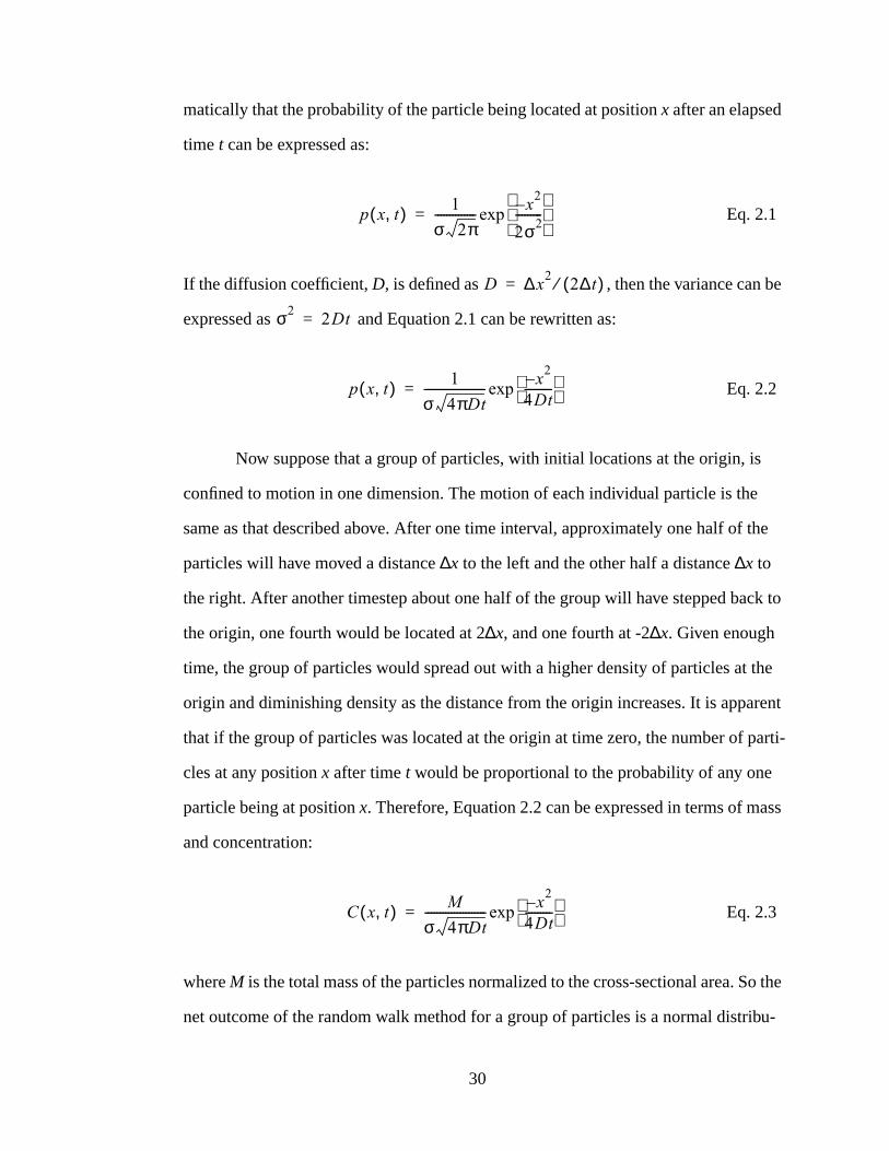
matically that the probability of the particle being located at position x after an elapsed

time t can be expressed as:

Eq. 2.1

If the diffusion coefficient, D, is defined as , then the variance can be

expressed as and Equation 2.1 can be rewritten as:

Eq. 2.2

Now suppose that a group of particles, with initial locations at the origin, is

confined to motion in one dimension. The motion of each individual particle is the

same as that described above. After one time interval, approximately one half of the

particles will have moved a distance ∆x to the left and the other half a distance ∆x to

the right. After another timestep about one half of the group will have stepped back to

the origin, one fourth would be located at 2∆x, and one fourth at -2∆x. Given enough

time, the group of particles would spread out with a higher density of particles at the

origin and diminishing density as the distance from the origin increases. It is apparent

that if the group of particles was located at the origin at time zero, the number of parti-

cles at any position x after time t would be proportional to the probability of any one

particle being at position x. Therefore, Equation 2.2 can be expressed in terms of mass

and concentration:

Eq. 2.3

where M is the total mass of the particles normalized to the cross-sectional area. So the

net outcome of the random walk method for a group of particles is a normal distribu-

p x t,( ) 1

σ 2π-------------- x

2–

2σ2---------

exp=

D ∆x2 2∆t( )⁄=

σ2 2Dt=

p x t,( ) 1

σ 4πDt--------------------- x

2–4Dt---------

exp=

C x t,( ) M

σ 4πDt--------------------- x

2–4Dt---------

exp=

30

tion of particles with a mean of zero and a standard deviation of . It is important

to note that the spreading of particles amounts to a net motion of particles from a

higher concentration to a lower concentration. Furthermore, Equation 2.3 is the same

result as that obtained by the solution of the one-dimensional diffusion equation.

2.2 Laminar Flow Models

The laminar flow models were constructed by extending the random walk

method described previously to three dimensions, and then adding advection and a

boundary reaction. Typically a two-dimensional, radial coordinate system is used to

describe a circular pipe. This is possible due to the symmetry of the pipe’s cross-sec-

tion and it usually results in simpler transport equations. However, the theory behind

the random walk method is more readily applied to a three-dimensional cartesian coor-

dinate system than a radial coordinate system. While this leads to more complicated

geometry, the complications involved with diffusion in the radial direction using the

random walk approach are avoided.

Transport Within the Bulk Flow

Transport within the bulk flow is a result of two processes; advection and diffu-

sion. Because the flow regime is laminar, transport in the lateral (cross-sectional)

directions occurs as a result of molecular diffusion only. The reason being that, in lam-

inar flow, streamlines are smooth and continuous. There are no turbulent eddies that

may contribute to transport in any way. Advection is only in the longitudinal direction,

therefore the only way a particle may move laterally is through molecular diffusion.

Transport in the longitudinal (along the length of the pipe) direction occurs by both

advection and diffusion. Incidentally, molecular diffusion in the longitudinal direction

is practically negligible in comparison to advection. The following equation is used to

describe the velocity profile for laminar flow conditions in a circular pipe:

2Dt

31

Eq. 2.4

where uc is the centerline (maximum) velocity of the pipe, a is the pipe radius and r is

the radial location of the particle.

The run time of the model is broken up into a number of timesteps of length ∆t.

For each timestep, every particle is subject to random motion in each of the three

dimensions according to the random walk theory. This random motion simulates trans-

port due to molecular diffusion. At every timestep, and for every particle, a random

number is generated for each of the three dimensions. In theory, the random numbers

would have a standard normal distribution (mean of zero and standard deviation of

one). Since the particle distribution was shown to have a mean of zero and a standard

deviation of according to Equation 2.3, each random number is multiplied by

the quantity , where D is the molecular diffusion coefficient.

Most random number generators produce uniform random numbers between -1

and 1. Therefore, an extra routine is required to convert them to standard normal vari-

ables. During an average simulation, the number of random numbers required is on the

order of 1010. The time spent converting each number to a standard normal variable is

therefore quite considerable. The Central Limit Theorem, however, shows that if

enough uniform random numbers are generated they will assume a normal distribu-

tion. The random number would then only have to be converted so that the standard

deviation is one. This is achieved by multiplying each random number by , a fairly

non-time consuming procedure. The end result, according to the Central Limit Theo-

rem, is: if a large number of uniform random variables between and are gen-

erated, they will assume a normal distribution with a mean of zero and a standard

deviation of one. Each random variable would then have to be multiplied by

so that transport occurs in accordance with the random walk theory.

As mentioned previously, advection occurs only in the longitudinal direction.

u r( ) uc ucra---

2–=

2Dt

2D∆t

3

3– 3

2D∆t

32

The radial position of each particle at the beginning of the timestep is used to calculate

the respective velocity according to Equation 2.4. The longitudinal location of the par-

ticle at the end of the timestep would be its beginning of timestep location, plus the

product of the velocity and ∆t, plus or minus any random motion due to diffusion

(which would most likely be negligible). In summary, transport in the bulk flow can be

expressed by the following set of equations:

Eq. 2.5

Eq. 2.6

Eq. 2.7

where y and z are the lateral directions, x is the longitudinal direction, and ξ1, ξ2, and

ξ3, are uniform random numbers between and . This set of equations is

applied to each particle in the bulk flow at every timestep. If a particle encounters the

pipe wall, it is reflected so that the angle of incidence equals the angle of reflection.

The distance the particle travels from the reflection point is the same distance that it

would have travelled beyond the pipe wall had it not been reflected.

Transport and Decay Within the Biofilm

Transport within the biofilm occurs by the process of molecular diffusion only.

The models used in this research assume that there is no advection within the pore

space of the biofilm. The application of the random walk method to transport within

the biofilm is the same for that for the bulk flow. The only difference is that the bulk

flow molecular diffusion coefficient, D, is different than the biofilm molecular diffu-

sion coefficient Db. The relationship between D and Db is not exactly understood and

y t ∆t+( ) y t( ) ξ1 2D∆t⋅+=

z t ∆t+( ) z t( ) ξ2 2D∆t⋅+=

x t ∆t+( ) x t( ) u r t,( ) ∆t⋅ ξ3 2D∆t⋅+ +=

3– 3

33

has been the subject of considerable research in the past. Zhang and Bishop in 1994

performed an intensive study that showed the relationships between the ratio Db/D,

biofilm porosity and tortuosity. Porosity is defined as the ratio of the pore volume to

the total biofilm volume and tortuosity is defined as the ratio of the effective (actual)

pore/capillary length to the biofilm thickness. The results of the study show that a gen-

eral definition for the biofilm diffusion coefficient, Db, is:

Eq. 2.8

where n is the porosity and τ is the tortuosity. The following equations describe trans-

port within the biofilm region:

Eq. 2.9

Eq. 2.10

Eq. 2.11

This set of equations is applied to each particle in the biofilm at every timestep.

In order to simulate the effects of a boundary reaction, any particle located

within the biofilm loses mass by either a first order or zero order reaction. The mass of

each particle decays according to the following equation for a zero order reaction:

Eq. 2.12

where k0 is the zero order reaction rate and ∆tbio is the length of time the particle is in

the biofilm. The particle may remain in the biofilm for the entire timestep, may leave

Dbn

τ2-----D=

y t ∆t+( ) y t( ) ξ1 2Db∆t⋅+=

z t ∆t+( ) z t( ) ξ2 2Db∆t⋅+=

x t ∆t+( ) x t( ) ξ3 2Db∆t⋅+=

Mass t ∆t+( ) Mass t( ) k0∆tbio–=

34

the biofilm at some time during the timestep, or may enter the biofilm at some point

during the timestep. If the reaction is first order, the following backward difference

equation is used to compute the decay of each particle in the biofilm (because the

timestep length is so short a linear approach to a non linear equation is acceptable):

Eq. 2.13

where k1 is the first order decay constant (a positive decay constant represents a

decay).

Bulk Flow - Biofilm Interface Condition

At any point within a given timestep, a particle may come in contact with the

bulk flow - biofilm interface. When this occurs, it has to be decided whether the parti-

cle will enter the biofilm or reflect off it and remain in the bulk flow. At the interface

there is no advection because the velocity of a fluid at a solid boundary must be zero

(in compliance with the no-slip condition). Therefore, molecular diffusion is the only

factor controlling the motion of the particle at the boundary. Since the molecular diffu-

sion coefficient is usually different for the two regions, the probability of the particle

diffusing to one side of the interface will be different than the probability of diffusion

to the other side. A probability rule was developed to make this determination.

Suppose a slug of tracer is injected at the boundary between two regions with

different molecular diffusion coefficients. After a given amount of time, the concentra-

tion profile will approach a distribution that is skewed to the side with the greater dif-

fusion coefficient. The percentage of the total mass residing in one of the two regions

represents the probability of any particular particle diffusing to that region. In other

words, if an equal percentage of mass is located in the two regions after a given

amount of time, then a particle located at the interface has the same probability of dif-

Mass t ∆t+( ) Mass t( ) k1Mass t( )∆tbio–=

35

fusing to one side of the interface as the other side. If 75% of the mass is located to the

left of the interface, then a particle located at the interface has a 75% chance of diffus-

ing to left and a 25% chance of diffusion to the right. This probability must be

expressed in terms of the biofilm and bulk flow characteristics if it is to be used for

modeling purposed. This is accomplished through the solution of the diffusion equa-

tion in an infinite 2-region medium with the interface at x=0. Since the timestep used

in the particle tacking model is very small, the new position of a particle originating at

the interface will be close to the interface itself. The influence of other boundaries is

not felt during a small timestep. Thus, it is reasonable to develop a probability rule for

determining the particle position assuming an infinite medium on either side of the

interface.

The one-dimensional diffusion equation for a two region system with the inter-

face at the origin (x = 0) is written as:

Eq. 2.14

The two boundary conditions for this set of equations are: equal concentrations at the

interface and equal flux at the interface. If region 1 is the bulk flow and region 2 is the

biofilm, then n is equal to 1.0 when x > 0 and D1 and D2 can be referred to as D and

Db, respectively. Solving Equation 2.14 using the new notation for the percent mass in

the bulk flow, results in the following expression for p (the probability that a particle

located at the bulk flow - biofilm interface will diffuse into the bulk):

Eq. 2.15

where n is the porosity of the biofilm. For use in the model, p must be rescaled so that

a probability of zero is represented by -1 and a probability of one is represented by 1

C∂t∂

------- nD1x

2

2

∂∂ C

Region 1 - x > 0,=

C∂t∂

------- nD2x

2

2

∂∂ C

Region 2 - x < 0,=

p 1

1 n Db D⁄+--------------------------------=

36

because the random number generator generates random numbers with a uniform dis-

tribution between -1 and 1. The rescaled probability will be denoted, pn.

During a model simulation, if a particle reaches the interface (whether coming

from the biofilm or the bulk flow), a random number between -1 and 1 is generated. If

the random number is greater than pn, the particle will diffuse into the biofilm. If the

random number is less than pn, the particle will diffuse into the bulk flow. Therefore, if

the probability of a particle diffusing to the bulk flow is 1.0, then no particle will enter

the biofilm because a random number greater than 1.0 will never be generated. If the

probability of a particle diffusing to the bulk flow is 0.5 (represented as 0.0 when

rescaled to pn), then the particle has an equal chance of entering the biofilm as the bulk

flow (because half the time the random number will be greater than 0.0 and half the

time less than 0.0). As shown in Equation 2.15, the probability rule is a function of

porosity and the ratio D/Db. To give an example of the effects of porosity on the parti-

cle behavior at the interface, assume that the biofilm porosity is zero. If this is the case,

a particle should never enter the biofilm because there is no available pore space in

which to go. Equation 2.15 computes a probability of 1, so the particle will never enter

the biofilm. Now assume that the porosity of the biofilm is 1 (this is the same porosity

as the bulk flow) and the diffusion coefficients for both regions are equal (D/Db =1).

We would expect that a particle located at the interface would diffuse to either region

with equal probability because the characteristics of both regions are the same. For this

case the probability, p, is 0.5 (rescaled to pn = 0.0), so the particle will behave as

expected. This probability rule ensures that particles will behave accordingly at the

interface.

Timestep Restrictions

The random walk method of particle tracking is only accurate when certain

restrictions are placed on the timestep (∆t) and the size of the typical displacement by

37

diffusion (∆x) during ∆t. Both ∆t and ∆x must be several orders of magnitude smaller

than the total time and space scale of the simulation. The time and space intervals must

also be much smaller than those of any physical phenomenon occurring within the sys-

tem. For example, the time and space intervals would have to be much smaller than

those of any turbulent eddies that may exist in the system in order to fully capture their

effects on transport.

Since, the distance travelled by any particle in a given timestep is directly

related to the timestep length, it is only necessary to restrict the timestep length used in

simulation. As stated above, the time interval, ∆t, must be much smaller than the

observation time and must be small enough so that the diffusion step is much smaller

than observation space. Therefore, the timestep should be limited so that the largest

diffusion step (space interval) is smaller than 1% of the pipe radius. The largest possi-

ble diffusion step is where is the largest random number generated.

This restriction takes the following form:

Eq. 2.16

Also, a particle should not be able to diffuse through the entire depth of the biofilm in

any timestep. To be conservative, this restriction limits the space interval to half the

biofilm thickness and takes the following form:

Eq. 2.17

where bt is the biofilm thickness. Finally, the timestep must be much smaller than the

timescale associated with decay in the biofilm. Therefore ∆t << 1/k1 where k1 is the

first order decay constant.

3 2D∆t 3

∆t0.01a( )2

6D---------------------<

∆t0.5bt( )2

6Db-------------------<

38

2.3 Turbulent Flow Models

The extension of the random walk method to turbulent flow in a pipe is slightly

more complicated. Transport and reaction within the biofilm remains the same and the

interface condition still holds true, but some changes are required in the description of

the bulk flow mass transport. Since rotational eddies exist in a turbulent flow field,

transport in the lateral directions is no longer only a result of molecular diffusion. A

cross-sectional mixing coefficient, termed the eddy diffusivity, has to be developed to

replace the diffusion coefficient in the transport equations. Unlike the diffusion coeffi-

cient, the eddy diffusivity is a function of the particle’s radial location. Also, a differ-

ent velocity profile will have to be developed that applies to turbulent flow within a

circular pipe. The universal velocity profile, otherwise known as the logarithmic veloc-

ity profile (discussed in Chapter 1), accurately describes the velocity field in the turbu-

lent core. Finally, boundary layer theory and experimentation show that a laminar

sublayer exists between the pipe wall and the turbulent core. In the laminar subregion,

which is usually extremely thin, transport occurs as a result of molecular diffusion.

Therefore, the diffusivity will have to be adjusted for this region. Furthermore, a dif-

ferent velocity profile is required for the laminar sublayer. A description of the back-

ground theory to turbulent flow as it applies to Taylor dispersion can be found in

Chapter 1.

Mass Transport in the Vicinity of the Pipe Wall

Typically when describing fully turbulent flow within a pipe, the flow regime is

divided into three distinct zones; the laminar sublayer, a buffer zone, and the turbulent

core. In the turbulent core, which encompasses the vast majority of the flow regime,

inertial forces dominate and viscous forces can be neglected. This is the standard defi-

nition of turbulent flow. As discussed previously, laminar boundary layer theory dic-

tates that near a solid boundary the viscous forces must become significant at least

39

within some small region near the boundary. In turbulent flow, the region where vis-

cous forces cannot be neglected consists of both the laminar sublayer and the buffer

zone. In the laminar sublayer, viscous forces dominate and inertial forces can be

neglected. In the buffer zone, both viscous and inertial forces must be retained. The

logarithmic law can be used to specify the velocity profile in each of the zones thus

resulting in a continuous velocity profile across the pipe cross section.

While the analysis just described is useful for determining turbulent flow

velocities, it is not valid for describing turbulent transport in the vicinity of the pipe

wall. The concept of three different fluid layers leads to an unrealistic discontinuity in

the eddy diffusivity function. While the three separate functions to describe the veloci-

ties in each layer are continuous, their first derivatives, which are used to calculate the

eddy diffusivity, are not continuous. Furthermore, the Reynold’s analogy, which is

used to derive expressions for the eddy diffusivity, breaks down near the wall. The

Reynold’s analogy for turbulent flow assumes that transport of mass is equal to trans-

port of momentum. This relationship is expressed by the Schmidt number, defined as

follows for the laminar region:

Eq. 2.18

where D is the molecular diffusion coefficient and υ is the kinematic viscosity. For the

Reynold’s analogy to be valid, the Schmidt number has to equal one, which obviously

would not be the case in the laminar sublayer. Therefore, in order to effectively

describe mass transfer near the pipe wall, the Reynold’s analogy must be abandoned

near the wall region (it still is valid in the turbulent core) and expressions for the veloc-

ity and eddy diffusivity that are continuous with the turbulent core must be developed.

In 1963, Wasan, Tien, and Wilke pointed out that most of the proposed eddy

viscosity distributions do not satisfy the theoretical criterion which stated that the tur-

Sc momentum transportmass transport

-------------------------------------------------- υD----= =

40

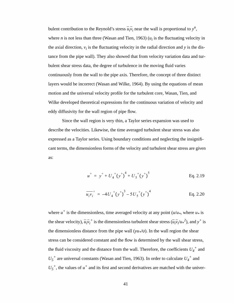
bulent contribution to the Reynold’s stress uivi near the wall is proportional to yn,

where n is not less than three (Wasan and Tien, 1963) (ui is the fluctuating velocity in

the axial direction, vi is the fluctuating velocity in the radial direction and y is the dis-

tance from the pipe wall). They also showed that from velocity variation data and tur-

bulent shear stress data, the degree of turbulence in the moving fluid varies

continuously from the wall to the pipe axis. Therefore, the concept of three distinct

layers would be incorrect (Wasan and Wilke, 1964). By using the equations of mean

motion and the universal velocity profile for the turbulent core, Wasan, Tien, and

Wilke developed theoretical expressions for the continuous variation of velocity and

eddy diffusivity for the wall region of pipe flow.

Since the wall region is very thin, a Taylor series expansion was used to

describe the velocities. Likewise, the time averaged turbulent shear stress was also

expressed as a Taylor series. Using boundary conditions and neglecting the insignifi-

cant terms, the dimensionless forms of the velocity and turbulent shear stress are given

as:

Eq. 2.19

Eq. 2.20

where u+ is the dimensionless, time averaged velocity at any point (u/u*, where u* is

the shear velocity), uivi+ is the dimensionless turbulent shear stress (uivi/u*

2), and y+ is

the dimensionless distance from the pipe wall (yu*/υ). In the wall region the shear

stress can be considered constant and the flow is determined by the wall shear stress,

the fluid viscosity and the distance from the wall. Therefore, the coefficients U4+ and

U5+ are universal constants (Wasan and Tien, 1963). In order to calculate U4

+ and

U5+, the values of u+ and its first and second derivatives are matched with the univer-

u+

y+

U 4+

y+( )

4U 5

+y

+( )5

+ +=

uivi+

4U 4+

y+( )

35U 5

+y

+( )4

––=

41

sal velocity profile in the turbulent core. This results in a smooth transition at y+ equal

to 19.7138. Using the calculated values for the coefficients, Equation 2.19 can be

rewritten to describe the velocity distribution for y+ < 19.7138:

Eq. 2.21

Likewise, Equation 2.20 can be rewritten to describe the time averaged turbulent shear

stress for y+ < 19.7138:

Eq. 2.22

Using Equation 2.21 and Equation 2.22, the following expression for the ratio of eddy

diffusivity (or eddy viscosity) to kinematic viscosity is given as:

Eq. 2.23

Equation 2.23 gives the distribution of the eddy diffusivity for the wall region (y+ <

19.7138). It results in a smooth transition to the eddy diffusivity in the turbulent core.

Expressions for the velocity and eddy diffusivity in the turbulent core are developed in

the following section.

Mass Transport in the Turbulent Core

As discussed previously, the universal velocity profile accurately describes the

velocity in the turbulent core. From Equation 1.15, the velocity is expressed as:

Eq. 2.24

u+

y+ 1.09833 10 4–

y+( )

4⋅– 3.30083 10 6–

y+( )⋅

5+=

uivi+

4.39332 10 4–y

+( )3

16.5041 10 6–y

+( )4

⋅–⋅=

ευ---

uivi+

u+

d y+

d⁄--------------------- 4.39332 10 4–

y+( )

316.5041 10 6–

y+( )

4⋅–⋅

1 4.39332 10 4–y

+( )3

16.5041 10 6–y

+( )4

⋅+⋅–----------------------------------------------------------------------------------------------------------------= =

u+ 5.5 2.5 y

+ln+=

42

From the Reynold’s analogy, the eddy diffusivity in the turbulent core is defined as

(from Equation 1.16):

Eq. 2.25

where ε is the eddy diffusivity, m is the rate of radial transfer of matter of concentra-

tion C, τ is the shear stress, τw is the wall shear stress, r is the radial coordinate, a is the

pipe radius, and ρ is the fluid density.

To be consistent with Equation 2.24 and the expressions for velocity and diffu-

sivity in the wall region, the diffusivity in the turbulent core should be expressed in

terms of y+. Using Equation 2.24, Equation 2.25 and the following definitions:

and , the ratio of eddy diffusivity to kinematic viscos-

ity can be expressed as:

Eq. 2.26

Equation 2.26 gives the eddy diffusivity distribution from y+ > 19.7138 to the center of

the pipe.

Velocity and Diffusivity Profiles

Figure 2.1 shows the velocity distribution from the wall to the pipe axis using

Equation 2.21 and Equation 2.24.

ε mC∂ r∂⁄

----------------– τ

ρ u∂r∂

-------------- υ–

τw r a⁄( )

ρ u∂r∂

-------------------------– υ–=–= =

τw u*2ρ= y

+a r–( )u* υ⁄=

ευ--- 0.4 y

+ 1 y+υ

au*---------–

1–=

43

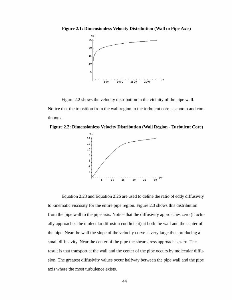
Figure 2.1: Dimensionless Velocity Distribution (Wall to Pipe Axis)

Figure 2.2 shows the velocity distribution in the vicinity of the pipe wall.

Notice that the transition from the wall region to the turbulent core is smooth and con-

tinuous.

Figure 2.2: Dimensionless Velocity Distribution (Wall Region - Turbulent Core)

Equation 2.23 and Equation 2.26 are used to define the ratio of eddy diffusivity

to kinematic viscosity for the entire pipe region. Figure 2.3 shows this distribution

from the pipe wall to the pipe axis. Notice that the diffusivity approaches zero (it actu-

ally approaches the molecular diffusion coefficient) at both the wall and the center of

the pipe. Near the wall the slope of the velocity curve is very large thus producing a

small diffusivity. Near the center of the pipe the shear stress approaches zero. The

result is that transport at the wall and the center of the pipe occurs by molecular diffu-

sion. The greatest diffusivity values occur halfway between the pipe wall and the pipe

axis where the most turbulence exists.

44

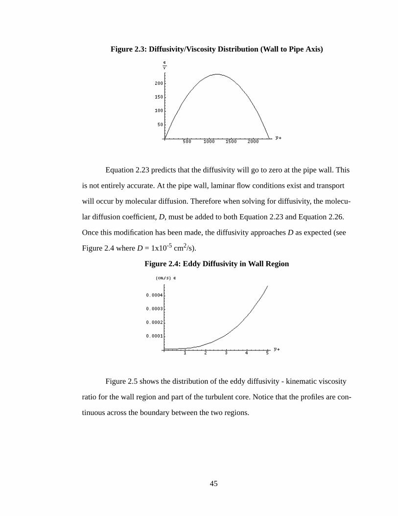
Figure 2.3: Diffusivity/Viscosity Distribution (Wall to Pipe Axis)

Equation 2.23 predicts that the diffusivity will go to zero at the pipe wall. This

is not entirely accurate. At the pipe wall, laminar flow conditions exist and transport

will occur by molecular diffusion. Therefore when solving for diffusivity, the molecu-

lar diffusion coefficient, D, must be added to both Equation 2.23 and Equation 2.26.

Once this modification has been made, the diffusivity approaches D as expected (see

Figure 2.4 where D = 1x10-5 cm2/s).

Figure 2.4: Eddy Diffusivity in Wall Region

Figure 2.5 shows the distribution of the eddy diffusivity - kinematic viscosity

ratio for the wall region and part of the turbulent core. Notice that the profiles are con-

tinuous across the boundary between the two regions.

45

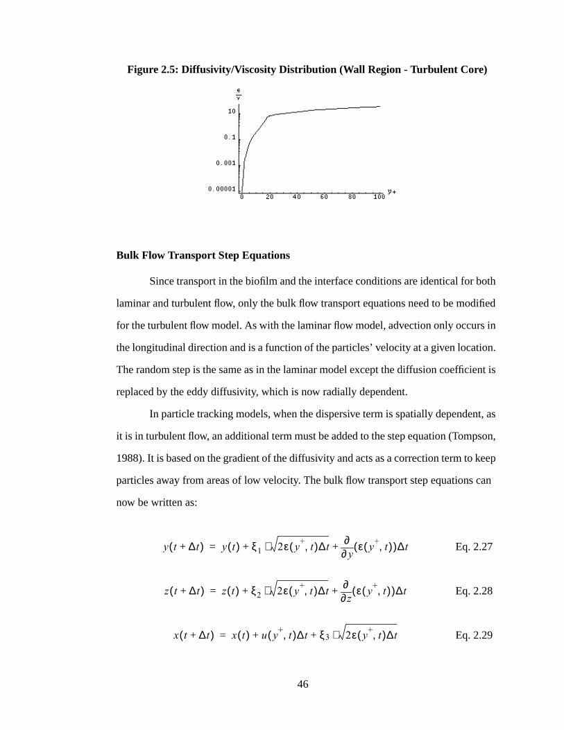
Figure 2.5: Diffusivity/Viscosity Distribution (Wall Region - Turbulent Core)

Bulk Flow Transport Step Equations

Since transport in the biofilm and the interface conditions are identical for both

laminar and turbulent flow, only the bulk flow transport equations need to be modified

for the turbulent flow model. As with the laminar flow model, advection only occurs in

the longitudinal direction and is a function of the particles’ velocity at a given location.

The random step is the same as in the laminar model except the diffusion coefficient is

replaced by the eddy diffusivity, which is now radially dependent.

In particle tracking models, when the dispersive term is spatially dependent, as

it is in turbulent flow, an additional term must be added to the step equation (Tompson,

1988). It is based on the gradient of the diffusivity and acts as a correction term to keep

particles away from areas of low velocity. The bulk flow transport step equations can

now be written as:

Eq. 2.27

Eq. 2.28

Eq. 2.29

y t ∆t+( ) y t( ) ξ1 2ε y+

t,( )∆ty∂

∂ ε y+

t,( )( )∆t+⋅+=

z t ∆t+( ) z t( ) ξ2 2ε y+

t,( )∆tz∂

∂ ε y+

t,( )( )∆t+⋅+=

x t ∆t+( ) x t( ) u y+

t,( )∆t ξ+ 3 2ε y+

t,( )∆t⋅+=

46

For the step term in the axial direction, the value for the lateral diffusivity is used. It is

assumed that the lateral diffusivity is equal to the longitudinal diffusivity. Also, the dif-

fusivity gradient correction term is not necessary in the axial direction.

Timestep Restrictions

For turbulent flow, the time-space restrictions are similar to those of the lami-

nar flow model. However, since turbulent flow contains eddies, and transport in the lat-

eral direction is a result of these eddies and internal turbulence, the timestep much be

much smaller than for laminar flow in order to capture this physical phenomenon.

As in laminar flow, the timestep must be much smaller that 1/k1 in order to rep-

resent exponential decay with a linear approximation. Also, a particle should not be

able to travel across the entire biofilm in a single timestep. Therefore, to be conserva-

tive:

Eq. 2.30

Finally, a particle should not be able to travel laterally more than a distance of 1% of

the radius in a single timestep. Lateral transport is a result of the eddy diffusivity and

the diffusivity gradient correction term. Therefore, ∆t must be chosen such that

Eq. 2.31

where is the maximum value of the random term, εmax is the maximum possible

value for the eddy diffusivity and is the maximum possible value for the

diffusivity gradient correction term. The timestep dictated by Equation 2.31 is almost

invariably the controlling factor in choosing the proper timestep length. Since the wall

region of the flow field is very thin, it is important that the timestep is small enough to

∆t0.5bt( )2

6Db-------------------<

0.01a 3 2εmax∆tε∂y∂

------

max∆t+>

3

ε∂ y∂⁄( )max

47

capture the detail of the velocity and diffusivity profiles in this region. However, the

dispersion coefficient in the wall region is very small (approaches the molecular diffu-

sion coefficient) so the timestep specified by Equation 2.31 is more than adequate to

ensure proper behavior in the wall region.

2.4 System Characterization

Various physical parameters are required to describe both the bulk flow and the

biofilm regions. The main parameters required to describe the bulk flow are the radius

of the pipe, the Reynold’s number, the molecular diffusion coefficient and the velocity

profile. The velocity profiles are dependant upon whether the flow is laminar or turbu-

lent and are described in detail previously. The radius of the pipe is basically chosen as

a matter of convenience depending upon a particular simulation. For the laminar flow

simulations, the pipe radius was chosen to be 0.8 cm unless otherwise specified. This

is the same value used for Tim Cox’s research and in the Horn and Hempel experi-

ments. The range of molecular diffusion coefficients given in literature is 10-4 to 10-6

cm/s (Chapra, 1997). Unless otherwise stated, the molecular diffusion coefficient was

chosen to be the average value of 10-5 cm/s. The Reynold’s number was varied over

several orders of magnitude for different simulations to show the dependence (or lack

thereof) of the transport parameters on Reynold’s number.

The physical parameters required to describe the biofilm coating are its thick-

ness, porosity, diffusion coefficient, and decay constant. Values given in literature for

typical biofilm thicknesses are in the range of 0.004 - 0.05 cm (Cox, 1997). For most

of the simulations, a biofilm thickness of 0.035 cm is used. This is the value used in the

Horn and Hempel experiments as well as Tim Cox’s research. However, a sensitivity

analysis is performed to show the effects of biofilm thickness on the bulk transport

parameters. Biofilm porosities are given in the range of 0.58 - 0.93 with an average of

0.7 - 0.75 (Zhang and Bishop 1, 1994). Unless otherwise stated, a porosity of 0.73 is

used in the simulations. Molecular diffusion in biofilms is usually described with a

48

ratio of the biofilm diffusion to bulk flow diffusion. This ratio is shown to be depen-

dant upon the biofilm porosity and tortuosity (Zhang and Bishop 2, 1994). Considering

the range of values given for porosity and tortuosity in biofilms, Equation 2.8 can be

used to calculate the possible values for the ratio of biofilm diffusion to bulk flow dif-

fusion. The calculated range is 0.36-0.81 with an average of 0.55-0.6. In the simula-

tions, the biofilm diffusion coefficient is chosen to be 60% of the bulk flow diffusion.

A sensitivity analysis is performed to show the model sensitivity to both porosity and

biofilm diffusion.

The rate constants used to describe the reactions occurring in the biofilm are

dependent upon both the makeup of the biofilm and the reactive constituent. Since

there is no particular type of solute or biofilm being studied in this research, there is no

specific range of values for the decay constant. In general, first order rate constants are

on the order of -1.0/s (Cox, 1997). The value used in simulation varies and will be

specified with the simulation results.

49

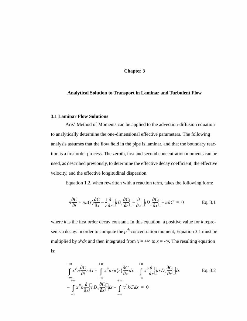
Chapter 3

Analytical Solution to Transport in Laminar and Turbulent Flow

3.1 Laminar Flow Solutions

Aris’ Method of Moments can be applied to the advection-diffusion equation

to analytically determine the one-dimensional effective parameters. The following

analysis assumes that the flow field in the pipe is laminar, and that the boundary reac-

tion is a first order process. The zeroth, first and second concentration moments can be

used, as described previously, to determine the effective decay coefficient, the effective

velocity, and the effective longitudinal dispersion.

Equation 1.2, when rewritten with a reaction term, takes the following form:

Eq. 3.1

where k is the first order decay constant. In this equation, a positive value for k repre-

sents a decay. In order to compute the pth concentration moment, Equation 3.1 must be

multiplied by xpdx and then integrated from x = +∞ to x = -∞. The resulting equation

is:

Eq. 3.2

nC∂t∂

------- nu r( ) C∂x∂

------- 1r---

r∂∂ nDr

C∂r∂

-------

x∂∂ nDx

C∂x∂

------- nkC–––+ 0=

xpn

C∂t∂

-------r xd

∞–

+∞

∫ xpnru r( ) C∂

x∂------- xd

∞–

+∞

∫ xp

r∂∂ nrDr

C∂r∂

------- xd

∞–

+∞

∫

xpn

x∂∂ rDx

C∂x∂

------- xd

+∞

∫ xpkC xd

+∞

∫––

–+

0=

∞– ∞–

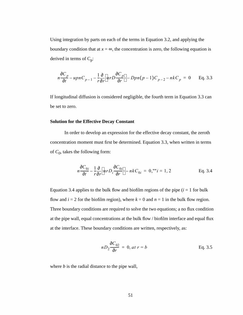
Using integration by parts on each of the terms in Equation 3.2, and applying the

boundary condition that at x = ∞, the concentration is zero, the following equation is

derived in terms of Cp:

Eq. 3.3

If longitudinal diffusion is considered negligible, the fourth term in Equation 3.3 can

be set to zero.

Solution for the Effective Decay Constant

In order to develop an expression for the effective decay constant, the zeroth

concentration moment must first be determined. Equation 3.3, when written in terms

of C0, takes the following form:

Eq. 3.4

Equation 3.4 applies to the bulk flow and biofilm regions of the pipe (i = 1 for bulk

flow and i = 2 for the biofilm region), where k = 0 and n = 1 in the bulk flow region.

Three boundary conditions are required to solve the two equations; a no flux condition

at the pipe wall, equal concentrations at the bulk flow / biofilm interface and equal flux

at the interface. These boundary conditions are written, respectively, as:

Eq. 3.5

where b is the radial distance to the pipe wall,

nC p∂t∂

---------- upnC p 1––1r---

r∂∂ nrD

C p∂r∂

---------- – Dpn p 1–( )C p 2–– nkC p– 0=

nC0i∂

t∂----------- 1

r---

r∂∂ nrDi

C0i∂r∂

----------- nkC0i–– 0 ""i 1 2,=,=

nD2

C02∂r∂

----------- 0 at r = b,=

51

Eq. 3.6

where a is the distance to the bulk flow / biofilm interface, and

Eq. 3.7

Using the discontinuous weighing function theory from boundary value problems in

heat conduction (which is analogous to mass transport in a fluid) the solution to Equa-

tion 3.4 can be written:

Eq. 3.8

where n is the eigenvalue index, Xin(r) are the radial eigenfunctions, Γin(t) describes

the temporal behavior associated with the nth eigenvalue, and An is a constant coeffi-

cient (Cox, 1997). Combining Equation 3.8 and Equation 3.4, the following expres-

sions are obtained:

Eq. 3.9

Eq. 3.10

where λin is the nth eigenvalue for either region 1 (bulk flow) or region 2 (biofilm). The

eigenvalues for the two regions are related as follows:

Eq. 3.11

C01 C02 at r = a,=

D1

C01∂r∂

-----------– nD2

C02∂r∂

----------- at r = a,–=

C0i r t,( ) An X in r( )Γ in t( ) i⇒n 1=

∞

∑ 1 2,= =

Γ1n t( ) λ1n2

t( )exp=

Γ2n t( ) λ2n2

k–( )t( )exp=

X 1n r( ) J 0 β1nr( )=

X 2n r( ) C2nI 0 β2nr( ) B2nK0 β2nr( )+=

λ1n2 λ2n

2k–=

52

where λ1n2 must be less than zero and therefore λ2n

2 must be less than k. In Equation

3.10, J0 is the zero order Bessel Function of the first and second kind and I0 and K0 are

the zero order, Modified Bessel Functions of the first and second kind, respectively.

β1n and β2n, used for simplicity, are defined as:

Eq. 3.12

C2n and B2n are constants that can be solved for by using the boundary conditions

defined by Equation 3.5 and Equation 3.6. The resulting expressions are given below

and can be solved simultaneously through substitution:

Eq. 3.13

Eq. 3.14

where I1 and K1 are first order Modified Bessel Functions of the first and second kind,

respectively.

The eigenvalues for the system can be determined by applying the equal flux

boundary condition, defined by Equation 3.7, to the expressions for C01 and C02

(Equation 3.4). The resulting transcendental equation is written as:

Eq. 3.15

where β1n and β2n are related by Equation 3.11. The roots of the transcendental equa-

tion are the eigenvalues for the system.

The remaining unknown coefficient from Equation 3.8, An, is solved for using

the Orthogonal-Expansion Technique from heat transport. The reader is referred to

β1n λ1n2

– D1⁄=

β2n λ2n2

D2⁄=

C2n

B2nK1 β2nb( )I 1 β2nb( )

---------------------------------=

B2n

J 0 β1na( ) C2nI 0 β2na( )–

K0 β2na( )------------------------------------------------------------=

D1β1nJ 1 β1na( ) n2D2β2n C2nI 1 β2na( ) B2nK1 β2na( )–( )–=

53

Cox, 1997 for the details of this solution, which will not be discussed here. The solu-

tion for An is of the following form:

Eq. 3.16

where f1 and f2 are the initial conditions for C0 for the bulk flow and the biofilm region,

respectively.

The above expressions can be used to reach a solution for C0. A computer code

is used to determine the eigenvalues that solve the equations. Since C0 gives the con-

centration moment at a single position r, it must be integrated over the pipe cross sec-

tion to determine the mass moment, M0:

Eq. 3.17

Then using Equation 1.21 the following expression can be derived for the

effective one-dimensional decay constant:

Eq. 3.18

After a large enough development time, the effective decay coefficient reaches an

asymptotic value. When this occurs, it can be seen that k* converges on λ12 where λ1 is

the region 1 eigenvalue closest to 0.0.

An

f 1J 0 β1nr( )r rd

0

a

∫ n2 f 2 C2nI 0 β2nr( ) B2nK0 β2nr( )+( )r rd

a

b

∫+

J 02 β1nr( )2

r rd

0

a

∫ n2 C2nI 0 β2nr( ) B2nK0 β2nr( )+( )2r rd

a

b

∫+

-------------------------------------------------------------------------------------------------------------------------------------------------=

M 0 2πAn λ1n2( ) a

β1n--------J 1 β1na( )⋅exp

n 1=

∞

∑=

k*

t( )dM 0 dt⁄

M 0--------------------

2πAn λ1n2( ) a

β1n--------J 1 β1na( )λ1n

2⋅expn 1=

∞

∑

2πAn λ1n2( ) a

β1n--------J 1 β1na( )⋅exp

n 1=

∞

∑--------------------------------------------------------------------------------------------= =

54

Solution for Effective Velocity

To solve for the first moment of concentration, Equation 3.3 takes the form:

Eq. 3.19

The same boundary conditions apply as described by Equation 3.5, Equation 3.6, and

Equation 3.7. The solution, again from heat conduction theory, is written as:

Eq. 3.20

Because the same boundary conditions exist for this problem, the spatial solu-

tion is the same as that derived for C0. Plus, the application of the boundary condition

described by Equation 3.7 (equal flux at the interface between regions), assures that

the eigenvalues will be the same (Cox, 1997). Therefore, the spatial solution is written

as:

Eq. 3.21

where λ1 is the eigenvalue closest to 0.0.

The temporal solution to the problem is written as:

Eq. 3.22

where L is expressed as:

nC1i∂

t∂----------- unC0i–

1r---

r∂∂ nrDi

C1i∂r∂

----------- nkC1i–– 0 i⇒ 1 2,= =

C1i r t,( ) X in r( )Γ in t( ) i⇒n 1=

∞

∑ 1 2,= =

X 1 r( ) J 0

λ12

–

D1---------r

=

Γ1 t( ) λ12t( )Ltexp=

55

Eq. 3.23

Integrating the equation for C1 over the cross sectional area of the pipe, the fol-

lowing expression is obtained for the first moment of mass:

Eq. 3.24

From Equation 1.23 and Equation 3.17 the position of the centroid is:

Eq. 3.25

and applying Equation 1.24, the effective velocity is:

Eq. 3.26

Solution for the Effective Dispersion Coefficient

Equation 3.3, when used to solve for the second concentration moment, can be

written as:

Eq. 3.27

To develop expressions for the effective dispersion coefficient is it necessary to use the

full expressions for C0, C1 and C2. Applying integral transforms to these equations

results in a system of analytical expressions that can be used to determine D*. The

L

An u1 r( )J 02 β1r( )r rd

0

a

∫

J 02 β1r( )r rd

0

a

∫---------------------------------------------------=

M 1 2π λ12t( )Lt

aβ1-----J 1 β1a( )

exp=

X LtAn------=

U effXdtd

------- LAn------= =

nC2i∂

t∂----------- 2unC1i–

1r---

r∂∂

nrDi

C2i∂r∂

----------- – 2DinC0i– nkC2i– 0=

56

eigenvalues are the same as those used in the C0 solution.

3.2 Turbulent Flow Solution

A set of analytical solutions for the effective, one-dimensional transport

parameters in a turbulent flow setting with a boundary reaction is too complicated to

derive. Therefore, the turbulent flow model with the reactive biofilm cannot be verified

analytically. However, an analytical expression can be developed for the effective dis-

persion coefficient in turbulent flow when there is no biofilm. Hence, the particle

tracking model will be verified for the non-reactive case only. The extension to include

a boundary reaction will be presumed to be correct.

The following solution for the effective dispersion coefficient was developed

by Taylor in 1954 and was summarized by Fischer in 1979. A solvable form of the

advection-dispersion equation for turbulent flow, when written with a coordinate sys-

tem whose origin moves at the mean flow velocity, is given below (Fischer, 1979):

Eq. 3.28

where C is the cross-sectionally averaged concentration, C’ is the deviation from the

mean concentration (C - C), u’ is the deviation from the mean velocity (u - u), ξ = x -

ut (where x is the longitudinal direction), and ε is the eddy diffusivity as a function of

radial position. Solving Equation 3.28 for C’ results in the following expression:

Eq. 3.29

The rate of mass transport in the streamwise direction, relative to the moving

coordinate system, is expressed as:

Eq. 3.30

u'C∂ξ∂

------- 1r---

r∂∂

rε C'∂r∂

--------( )=

C'C∂x∂

------- 1rε----- u'r rd

0

r

∫

rd

0

r

∫ C' 0( )+=

M u'C'2πr rd

a

∫=

570

Combining Equation 3.29 and Equation 3.30 results in the following:

Eq. 3.31

the term because . The mass transport rate can also be

defined in terms of a bulk mass transport coefficient, which would be analogous to the

effective dispersion coefficient, by the following equation:

Eq. 3.32

Combining Equation 3.31 and Equation 3.32 and solving for D* gives the following

expression for the effective dispersion coefficient:

Eq. 3.33

Using the velocity and diffusivity profiles described in Section 2.3, and solving

Equation 3.33 through numerical integration, gives results that vary with the Reynolds

number, D* = f(Re)au*. Taylor’s 1954 analysis results in a value of 10.1au* for the

effective dispersion coefficient. This discrepancy is a result of the velocity profiles

used in the analysis. Taylor used a velocity profile that did not vary with Reynolds

number. Furthermore, the fact that the thickness of the laminar sublayer (wall region)

varies with Reynolds number was not accounted for. The velocity profile used in Equa-

tion 3.33 is the widely accepted, universal velocity profile which depends on the Rey-

nolds number. Also, the description of the wall region includes variations in thickness

dependent on the Reynolds number. Therefore, it is expected that Taylor’s result for

the effective dispersion coefficient is inconsistent with the solution to Equation 3.33.

M 2π C∂x∂

------- u'r1rε----- u'r rd rd rd

0

r

∫0

r

∫0

a

∫=

u'rC' 0( ) rd0

a

∫ 0= u'r rd0

a

∫ 0=

M πa2D

* C∂x∂

-------–=

D* 2

a2

-----–= u'r1rε----- u'r rd rd rd

0

r

∫0

r

∫0

a

∫

58

Chapter 4

Particle Tracking Results and Verification

For all particle tracking simulations the zeroth, first, and second mass moments

are calculated. These are used to compute the asymptotic values for the effective

decay, effective velocity, and the effective dispersion coefficients. Three plots are gen-

erated to determine the coefficients. The first is a plot of the zeroth moment versus

simulation time. In other words, it shows the total mass of the system as a function of

time. Since this is a first order decay process, an exponential curve can be fit to the

data to determine the rate constant. The first order rate constant is the bulk flow decay

coefficient.

The second plot shows the center of mass of the system as a function of time.

The center of mass is computed as the first moment of mass divided by the second

moment of mass. Once the pseudo steady state conditions have been established (the

initial development time has elapsed) the center of mass moves at a constant rate. This

is shown as a linear relationship between centroid position and time. The slope of this

line is the effective velocity.

The third plot shows the variance of the particle distribution as a function of

time. The variance is computed as:

Eq. 4.1 σ2 M 2

M 0-------- X

2t( )–=

After the initial development period, the variance changes at a constant rate. Once

again this is shown by a straight line on the graph. The slope of this line is equal to

twice the effective dispersion coefficient (see Equation 1.27).

4.1 Laminar Flow Results

Three simulations were run to give examples of the spatial moment curves and

to verify the particle tracking model with analytical results. Simulation 1 used the

average values for the biofilm parameters, a first order decay constant of -1.0, a molec-

ular diffusion coefficient of 1.0x10-5 cm2/s, and a mean bulk flow velocity of 6.44 cm/

s. Simulation 2 used all the same parameters, except a molecular diffusion coefficient

of 5.0x10-5 cm2/s. A simulation was also run with no decay occurring in the biofilm

(all other parameters are the same as simulations 1). Table 4.1 gives a summary of the

simulation results and the corresponding analytical solutions.

The particle tracking results match closely with the analytical solutions. While

there are some slight discrepancies, these simulations along with several others (some

if which are discussed later) suggest that the particle tracking model accurately

describes mass transport in a laminar flow field. There are several reasons why dis-

crepancies may occur. Since the effective transport coefficients are determined by

regression analyses of the moment curves, their values are subject to the degree of “fit”

of the regression curves. The regression analysis must be performed on the portion of

the moment curve that lies after the initial development period. If some of this region

Table 4.1: Comparison of Simulations to Analytical Results

Sim 1 Analytical 1 Sim 2 Analytical 2 No Decay

Keff (1/s) -9.79 x 10-5 -9.75 x 10-5 -4.85 x 10-4 -4.80 x 10-4 0.0

Ueff (cm/s) 9.93 10.03 9.82 9.90 6.10

Deff (cm2/s) 12533 12987 2802 2680 59519

60

is included in the regression analysis, the accuracy of the result may suffer, albeit very

slightly. Basically, the results of the regression analysis depend on the care taken by

the person performing them. An increase in the number of particles and a smaller

timestep would also lead to more accurate results. However, an effort was made to

used as few particles as possible and the largest timestep possible (that will still give

accurate results) in order to cut down on simulation run time. Finally, it is entirely pos-

sible that the analytical solutions are not exact. Due to the complex nature of the solu-

tion, which involves iteration, numerical solutions to find roots of equations, and the

summation of results from a theoretically infinite number of eigenvalues, the analytical

results themselves are only approximations.

For the same system as simulation 1 with no biofilm the effective decay coeffi-

cient is zero, the effective velocity is the mean flow velocity (6.44 cm/s), and the effec-

tive diffusion coefficient is 50565 cm2/s (from Equation 1.6). A reactive biofilm results

in a non-uniform concentration distribution across the pipe cross section because parti-

cles near the biofilm are subject to decay. Because this is also the region of lowest

velocity, the center of mass will travel faster than the mean velocity. Likewise the par-

ticles are subject to less separation because most of the mass exists in areas of lower

shear. As expected, Table 4.1 shows that the presence of a reactive biofilm causes the

effective velocity to increase and the effective dispersion coefficient to decrease. It is

interesting to note that the simulation with no decay results in a lower effective veloc-

ity than the mean flow and a higher effective dispersion than a pipe with no biofilm.

This is because particles may enter the biofilm without losing any mass. In the biofilm

the velocity is zero, so particles may lag behind the particles in the bulk flow. This

leads to a decreased effective velocity and an increase in particle separation.

It is important to notice that the effective decay coefficient is several orders of

magnitude smaller than the biofilm decay coefficient. Since the effective decay repre-

sents an overall decay of the mass in the bulk flow, it is expected to be much smaller

61

than the regional decay rate at the boundary.

The following figures are the spatial, mass moments resulting from simulations

1 and 2. The values reported in Table 4.1 are determined by a regression analysis of

these graphs. Figure 4.1 shows the change in mass as a function of time (M = mass and

Mt = total mass at the beginning of the simulation) for the two simulations. The effec-

tive decay coefficient is determined by fitting and exponential curve to the portion of

the curve that resides after the initial development time. The portion of the curve that

resides previous to the development time is not a first order function and therefore an

exponential curve could not be fit to it.

Figure 4.1: Zeroth Moment Curve

Figure 4.2 and Figure 4.3 can be used to investigate the development times for

the respective systems. The development region is a little more obvious in Figure 4.3

than Figure 4.2. It represented by the curved region of the graph before it develops into

a straight line. The development time for simulation 1 is approximately 5000 seconds.

It is difficult to determine the development time for simulation 2 but it is probably

about 1000 seconds. Because the molecular diffusion coefficient is greater for simula-

tion 2, mixing in the radial direction occurs faster. The initial distribution of particles

0.0 5000.0 10000.0 15000.0

Time (s)

0.0

0.2

0.4

0.6

0.8

1.0

M/M

t

Simulation 1 (D = 1e-5 cm2/s)Simulation 2 (D = 5e-5 cm2/s)

62

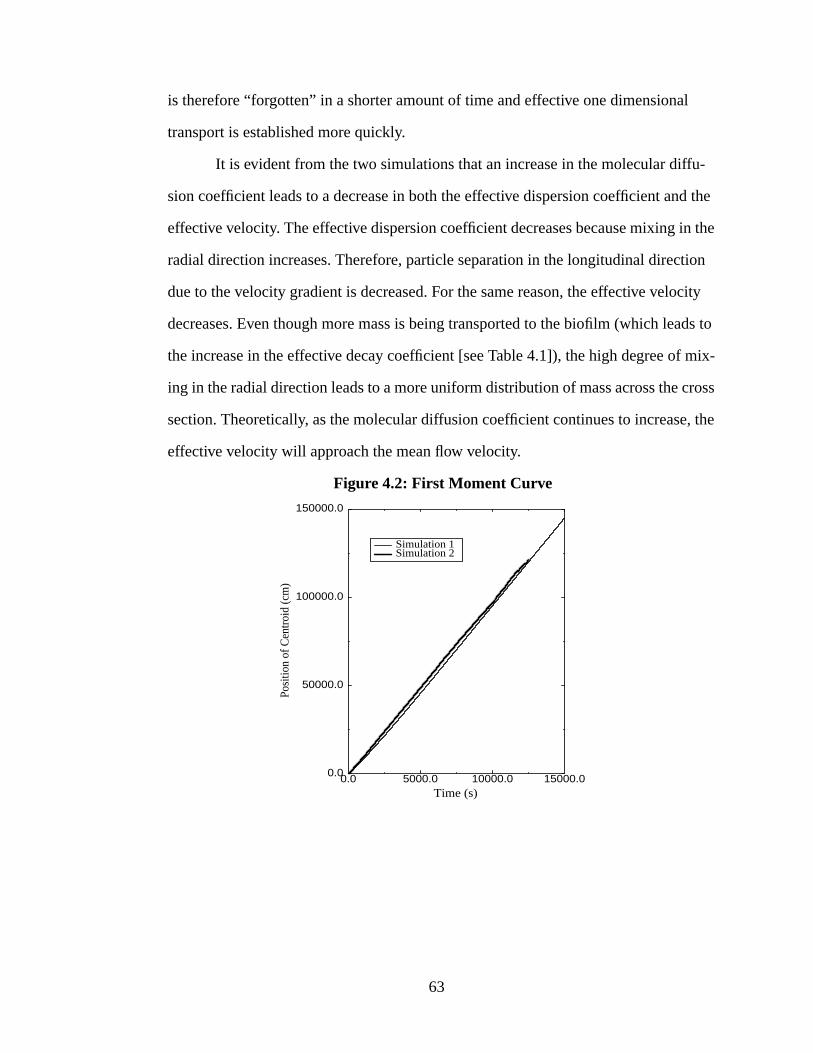
is therefore “forgotten” in a shorter amount of time and effective one dimensional

transport is established more quickly.

It is evident from the two simulations that an increase in the molecular diffu-

sion coefficient leads to a decrease in both the effective dispersion coefficient and the

effective velocity. The effective dispersion coefficient decreases because mixing in the

radial direction increases. Therefore, particle separation in the longitudinal direction

due to the velocity gradient is decreased. For the same reason, the effective velocity

decreases. Even though more mass is being transported to the biofilm (which leads to

the increase in the effective decay coefficient [see Table 4.1]), the high degree of mix-

ing in the radial direction leads to a more uniform distribution of mass across the cross

section. Theoretically, as the molecular diffusion coefficient continues to increase, the

effective velocity will approach the mean flow velocity.

Figure 4.2: First Moment Curve

0.0 5000.0 10000.0 15000.0Time (s)

0.0

50000.0

100000.0

150000.0

Posi

tion

of C

entr

oid

(cm

)

Simulation 1Simulation 2

63

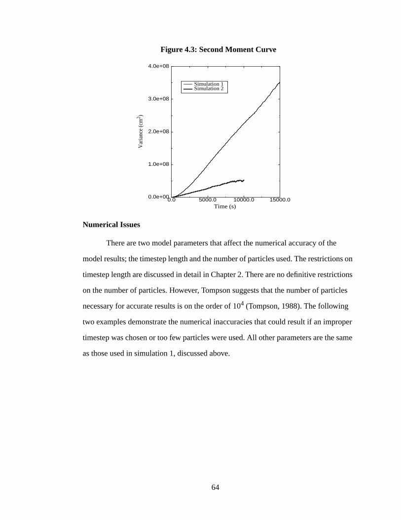
Figure 4.3: Second Moment Curve

Numerical Issues

There are two model parameters that affect the numerical accuracy of the

model results; the timestep length and the number of particles used. The restrictions on

timestep length are discussed in detail in Chapter 2. There are no definitive restrictions

on the number of particles. However, Tompson suggests that the number of particles

necessary for accurate results is on the order of 104 (Tompson, 1988). The following

two examples demonstrate the numerical inaccuracies that could result if an improper

timestep was chosen or too few particles were used. All other parameters are the same

as those used in simulation 1, discussed above.

0.0 5000.0 10000.0 15000.0Time (s)

0.0e+00

1.0e+08

2.0e+08

3.0e+08

4.0e+08

Var

ianc

e (c

m2 )

Simulation 1Simulation 2

64

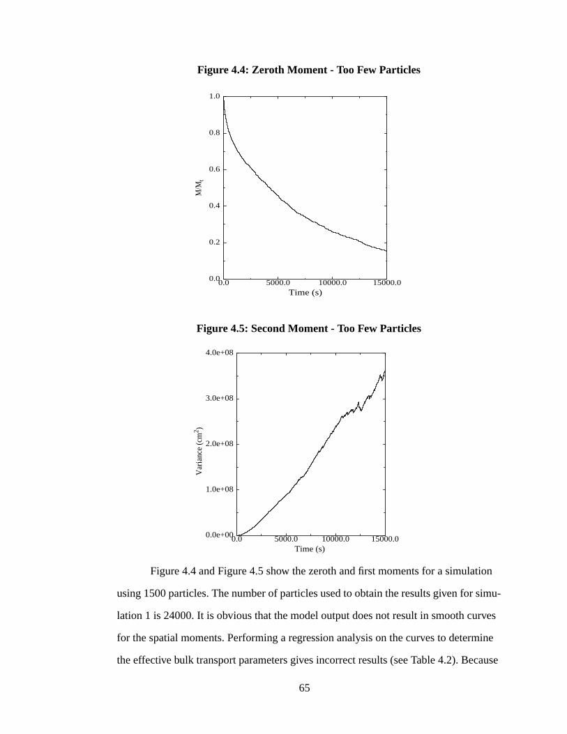
Figure 4.4: Zeroth Moment - Too Few Particles

Figure 4.5: Second Moment - Too Few Particles

Figure 4.4 and Figure 4.5 show the zeroth and first moments for a simulation

using 1500 particles. The number of particles used to obtain the results given for simu-

lation 1 is 24000. It is obvious that the model output does not result in smooth curves

for the spatial moments. Performing a regression analysis on the curves to determine

the effective bulk transport parameters gives incorrect results (see Table 4.2). Because

0.0 5000.0 10000.0 15000.0Time (s)

0.0

0.2

0.4

0.6

0.8

1.0

M/M

t

0.0 5000.0 10000.0 15000.0Time (s)

0.0e+00

1.0e+08

2.0e+08

3.0e+08

4.0e+08

Var

ianc

e (c

m2 )

65

the particles are behaving properly (i.e. a proper timestep was used), the discrepancy

between the model results and the correct results (those of simulation 1) is not consid-

erable. There are simply not enough particles for the mean motion to represent reality.

This explains why the spatial moments do not result in smooth curves. It would be

obvious to the model user that the results are not correct.

The simulation used to produce Figure 4.6 and Figure 4.7 used a timestep

length of 10 seconds when the appropriate timestep length (that used for simulation 1)

is approximately 0.1 seconds (as dictated by the time-space restrictions discussed in

Section 2.2). Unlike the results produced by a model with too few particles, a model

using an incorrect timestep will result in smooth curves for the spatial moments. As

long as there are a sufficient number of particles to get consistent and smooth average

particle transport, the moment curves will also be smooth. The behavior of the individ-

ual particle however, will be inconsistent with reality. For example, a particle could

move from the center of the pipe to the pipe wall in a single diffusion step. Therefore,

even though the spatial moment curves may look correct, a regression analysis of these

curves would give highly inaccurate values for the effective bulk transport coefficients.

The results in Table 4.2 show that this is indeed the case. A model user would have no

way of knowing that the results are inaccurate unless they were compared with an ana-

lytical model. Therefore, it is imperative that the timestep restrictions discussed in

Table 4.2: Discrepancies from IncorrectNumerical Parameters

Keff(x 10-5/s)

Veff(cm/s)

Deff(cm2/s)

Simulation 1 -9.79 9.80 12533

Too Few Particles -10.7 9.86 13197

Too Large ∆t -9.07 9.59 15831

66

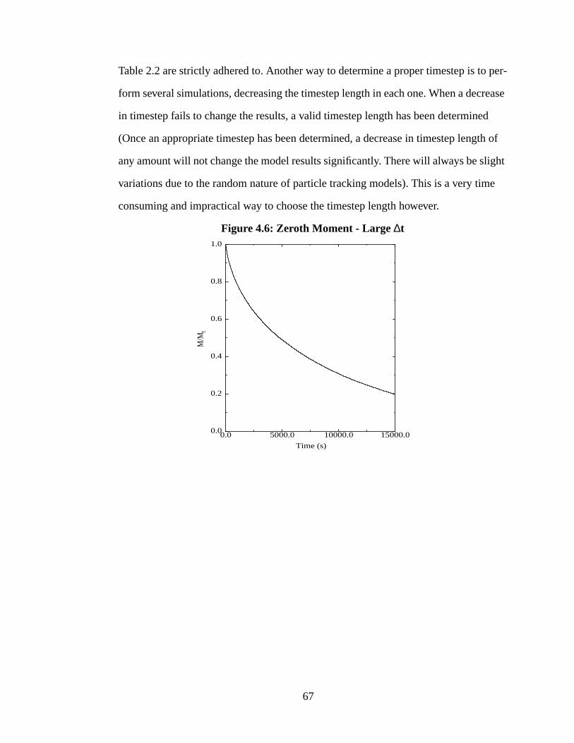
Table 2.2 are strictly adhered to. Another way to determine a proper timestep is to per-

form several simulations, decreasing the timestep length in each one. When a decrease

in timestep fails to change the results, a valid timestep length has been determined

(Once an appropriate timestep has been determined, a decrease in timestep length of

any amount will not change the model results significantly. There will always be slight

variations due to the random nature of particle tracking models). This is a very time

consuming and impractical way to choose the timestep length however.

Figure 4.6: Zeroth Moment - Large ∆t

0.0 5000.0 10000.0 15000.0

Time (s)

0.0

0.2

0.4

0.6

0.8

1.0

M/M

t

67

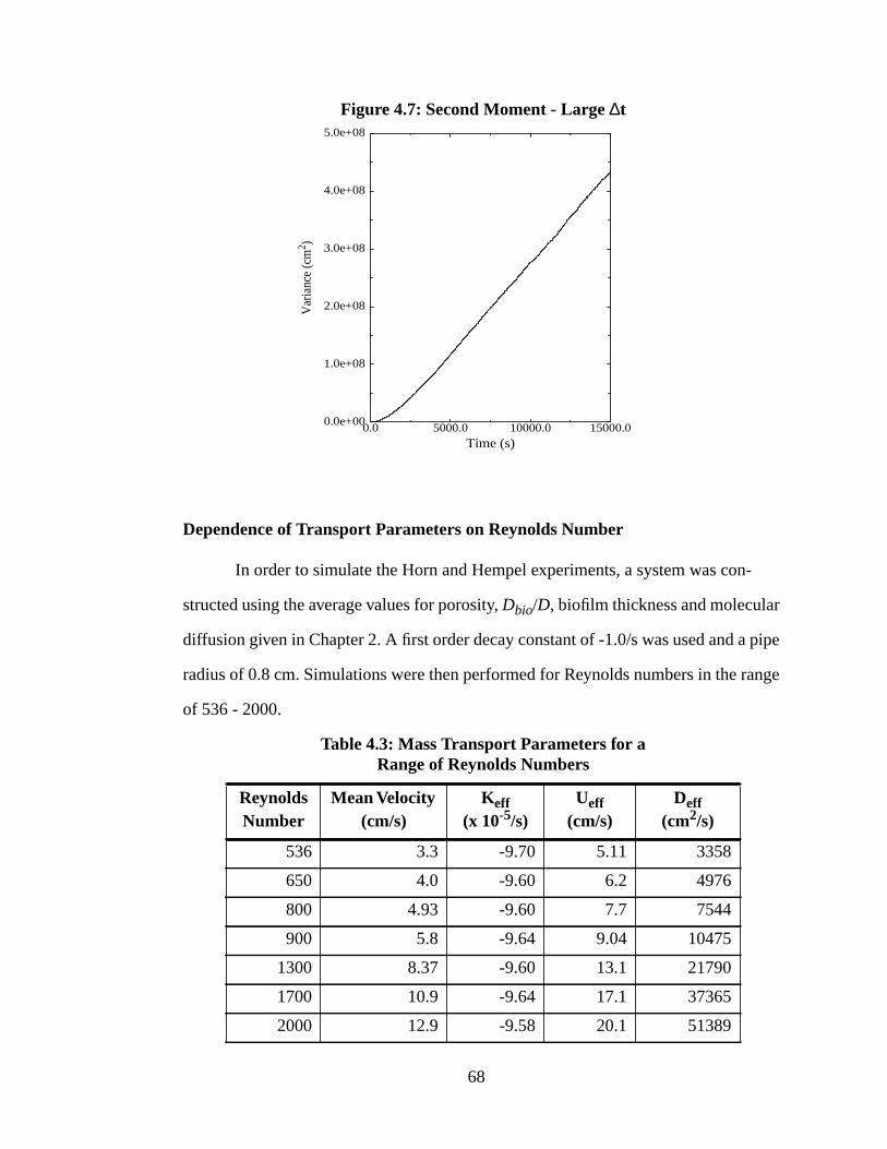
Figure 4.7: Second Moment - Large ∆t

Dependence of Transport Parameters on Reynolds Number

In order to simulate the Horn and Hempel experiments, a system was con-

structed using the average values for porosity, Dbio/D, biofilm thickness and molecular

diffusion given in Chapter 2. A first order decay constant of -1.0/s was used and a pipe

radius of 0.8 cm. Simulations were then performed for Reynolds numbers in the range

of 536 - 2000.

Table 4.3: Mass Transport Parameters for aRange of Reynolds Numbers

Reynolds Number

Mean Velocity (cm/s)

Keff(x 10-5/s)

Ueff(cm/s)

Deff(cm2/s)

536 3.3 -9.70 5.11 3358

650 4.0 -9.60 6.2 4976

800 4.93 -9.60 7.7 7544

900 5.8 -9.64 9.04 10475

1300 8.37 -9.60 13.1 21790

1700 10.9 -9.64 17.1 37365

2000 12.9 -9.58 20.1 51389

0.0 5000.0 10000.0 15000.0Time (s)

0.0e+00

1.0e+08

2.0e+08

3.0e+08

4.0e+08

5.0e+08

Var

ianc

e (c

m2 )

68

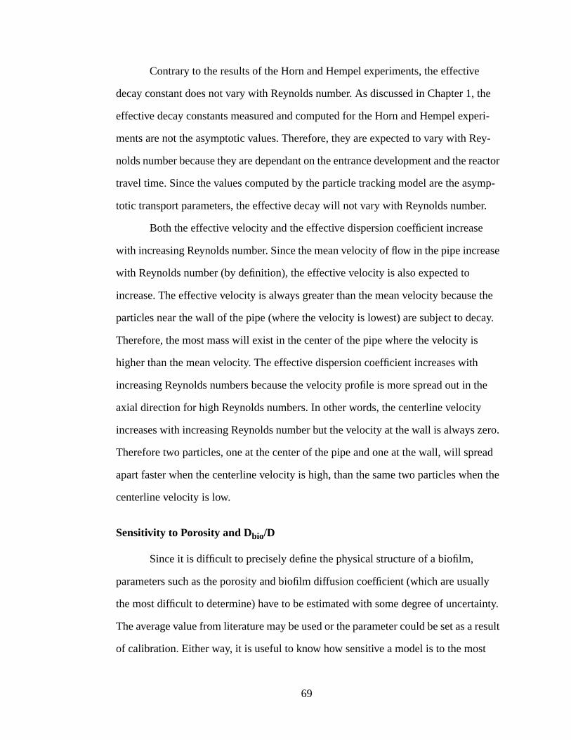
Contrary to the results of the Horn and Hempel experiments, the effective

decay constant does not vary with Reynolds number. As discussed in Chapter 1, the

effective decay constants measured and computed for the Horn and Hempel experi-

ments are not the asymptotic values. Therefore, they are expected to vary with Rey-

nolds number because they are dependant on the entrance development and the reactor

travel time. Since the values computed by the particle tracking model are the asymp-

totic transport parameters, the effective decay will not vary with Reynolds number.

Both the effective velocity and the effective dispersion coefficient increase

with increasing Reynolds number. Since the mean velocity of flow in the pipe increase

with Reynolds number (by definition), the effective velocity is also expected to

increase. The effective velocity is always greater than the mean velocity because the

particles near the wall of the pipe (where the velocity is lowest) are subject to decay.

Therefore, the most mass will exist in the center of the pipe where the velocity is

higher than the mean velocity. The effective dispersion coefficient increases with

increasing Reynolds numbers because the velocity profile is more spread out in the

axial direction for high Reynolds numbers. In other words, the centerline velocity

increases with increasing Reynolds number but the velocity at the wall is always zero.

Therefore two particles, one at the center of the pipe and one at the wall, will spread

apart faster when the centerline velocity is high, than the same two particles when the

centerline velocity is low.

Sensitivity to Porosity and Dbio/D

Since it is difficult to precisely define the physical structure of a biofilm,

parameters such as the porosity and biofilm diffusion coefficient (which are usually

the most difficult to determine) have to be estimated with some degree of uncertainty.

The average value from literature may be used or the parameter could be set as a result

of calibration. Either way, it is useful to know how sensitive a model is to the most

69

uncertain parameters. If it turns out that a model is very sensitive to these parameters,

then there would be justification in performing various experiments to measure them

in a more accurate manner. However, if it turns out that the model is not really affected

by these parameters, then it is probably safe to use an average value. Table 4.4 and

Table 4.5 show the sensitivity of the bulk transport parameters to porosity. All other

parameters are held constant at the average value discussed at the end of Chapter 2.

The radius of the pipe is 0.8 cm, the Reynolds number is 1000 and the first order decay

constant in the biofilm is -1.0.

Table 4.4 and Table 4.5 show that porosity does not have a significant impact

Table 4.4: Porosity Sensitivity Analysis - Particle Tracking Model

PorosityKeff

(x 10-5/s)Ueff

(cm/s)Deff

(cm2/s)

.4 -9.42 9.92 14220

.5 -9.85 9.92 13800

.65 -9.65 9.97 13300

.8 -9.77 10.05 12584

.95 -9.67 9.96 13115

1.0 -9.56 10.05 12307

Table 4.5: Porosity Sensitivity Analysis - Analytical Model

PorosityKeff

(x 10-5/s)Ueff

(cm/s)Deff

(cm2/s)

.4 -9.62 9.99 13042

.5 -9.67 10.01 12593

.65 -9.72 10.02 13106

.8 -9.75 10.03 12850

.95 -9.77 10.04 12677

1.0 -9.78 10.04 12656

70

on the bulk transport parameters. A change in porosity of ±43% (from the mean)

results in the following percent changes in the bulk transport parameters: ±0.8% in Keff

for the analytical model, ±2.2% in Keff for the particle tracking model, ±0.25% in Ueff

for the analytical model, ±0.65% change in Ueff for the particle tracking model, ±1.5%

in Deff for the analytical model, and ±7.5% in Deff for the particle tracking model.

While the bulk flow transport parameters appear to be relatively insensitive to

changes in porosity, there are some noticeable trends. An increase in porosity results in

an increase in Keff and Ueff, but a decrease in Deff. At higher porosities, particles are

able to enter the biofilm more readily. This is also reflected in the probability rule

expressed by Equation 2.15, and is consistent with the behavior expected due to

increased porosity of the biofilm. If more particles are allowed to enter the biofilm, the

effective decay coefficient would naturally increase. This results in less solute mass

near the biofilm (where the velocity is lowest and the shear is the greatest). Therefore,

the effective velocity increases and the effective dispersion decreases.

It is important to note that the particle tracking model is not accurate enough to

correctly predict the sensitivity to porosity. While it is still evident that the system is

relatively insensitive to changes in porosity, the trends shown in the analytical results

are not as obvious in the particle tracking results. In fact one could say that the particle

tracking model is unable to accurately portray these trends. The reason for this inaccu-

racy is the random nature of the model. Even with the same input parameters, the par-

ticle tracking model could return slightly different results (each simulation different

random numbers are generated). In this case, the differences caused by the random

nature of the model overshadow the differences caused by porosity variations. This

problem would be resolved by increasing the number of particles used in the simula-

tion.

Table 4.6 and Table 4.7 show the sensitivity of the bulk transport parameters to

the ratio of the biofilm diffusion coefficient to bulk flow diffusion coefficient (Dbio/D).

71

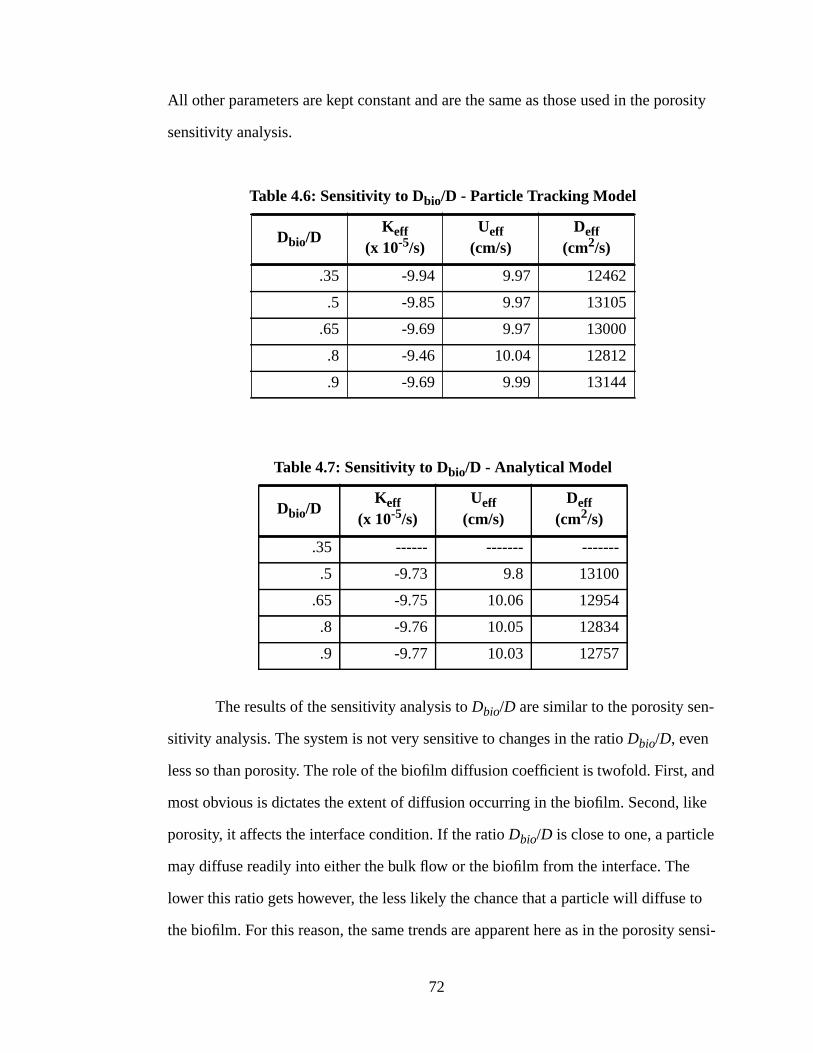
All other parameters are kept constant and are the same as those used in the porosity

sensitivity analysis.

The results of the sensitivity analysis to Dbio/D are similar to the porosity sen-

sitivity analysis. The system is not very sensitive to changes in the ratio Dbio/D, even

less so than porosity. The role of the biofilm diffusion coefficient is twofold. First, and

most obvious is dictates the extent of diffusion occurring in the biofilm. Second, like

porosity, it affects the interface condition. If the ratio Dbio/D is close to one, a particle

may diffuse readily into either the bulk flow or the biofilm from the interface. The

lower this ratio gets however, the less likely the chance that a particle will diffuse to

the biofilm. For this reason, the same trends are apparent here as in the porosity sensi-

Table 4.6: Sensitivity to Dbio/D - Particle Tracking Model

Dbio/DKeff

(x 10-5/s)Ueff

(cm/s)Deff

(cm2/s)

.35 -9.94 9.97 12462

.5 -9.85 9.97 13105

.65 -9.69 9.97 13000

.8 -9.46 10.04 12812

.9 -9.69 9.99 13144

Table 4.7: Sensitivity to Dbio/D - Analytical Model

Dbio/DKeff

(x 10-5/s)Ueff

(cm/s)Deff

(cm2/s)

.35 ------ ------- -------

.5 -9.73 9.8 13100

.65 -9.75 10.06 12954

.8 -9.76 10.05 12834

.9 -9.77 10.03 12757

72

tivity analysis. Once again, the particle tracking model is not sensitive enough to dis-

play these trends.

An important point to consider in this analysis is that the sensitivity results

apply to the specified system only. If the set of system parameters were to change, the

sensitivity analysis would also likely change. For example, the system just described is

mostly diffusion limited. This means that the bulk flow transport parameters are

largely affected by the rate at which solute can reach the biofilm. If the sensitivity anal-

ysis was performed on a rate limited system (the bulk flow transport parameters are

largely affected by the reaction rate in the biofilm), the results would show a greater

sensitivity to both porosity and Dbio/D. Likewise, a system with a thicker biofilm

would probably show greater sensitivity to Dbio/D than a system with a thin biofilm.

This hypothesis will be tested further in the next section.

Diffusion Limited Versus Rate Limited Systems

A diffusion limited system is one in which the ratio of the biofilm decay rate to

diffusive flux is high. In other words, the effective decay is governed by how fast mass

can be transported from the bulk flow into the biofilm where it would decay almost

instantly. When a system is limited by diffusion, an increase in the biofilm decay rate

does not have a significant effect on the bulk transport parameters. Conversely, in a

rate limited system, depleted mass is quickly replenished by diffusion from the bulk

flow. The ratio of the biofilm decay rate to diffusive flux is low. Therefore the bulk

flow effective decay is dictated by the decay rate in the biofilm.

It is believed that the system used to perform the previous sensitivity analysis

on porosity (shown in Table 4.4 and Table 4.5) was limited by diffusion. For compari-

son, the same analysis was performed for a rate limited system. The results are shown

in Table 4.8 and Table 4.9.

73

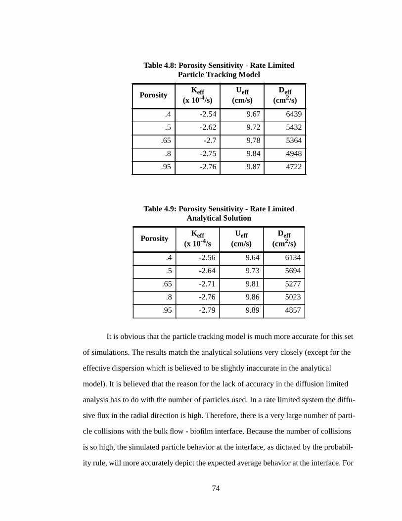
It is obvious that the particle tracking model is much more accurate for this set

of simulations. The results match the analytical solutions very closely (except for the

effective dispersion which is believed to be slightly inaccurate in the analytical

model). It is believed that the reason for the lack of accuracy in the diffusion limited

analysis has to do with the number of particles used. In a rate limited system the diffu-

sive flux in the radial direction is high. Therefore, there is a very large number of parti-

cle collisions with the bulk flow - biofilm interface. Because the number of collisions

is so high, the simulated particle behavior at the interface, as dictated by the probabil-

ity rule, will more accurately depict the expected average behavior at the interface. For

Table 4.8: Porosity Sensitivity - Rate LimitedParticle Tracking Model

PorosityKeff

(x 10-4/s)Ueff

(cm/s)Deff

(cm2/s)

.4 -2.54 9.67 6439

.5 -2.62 9.72 5432

.65 -2.7 9.78 5364

.8 -2.75 9.84 4948

.95 -2.76 9.87 4722

Table 4.9: Porosity Sensitivity - Rate LimitedAnalytical Solution

PorosityKeff

(x 10-4/sUeff

(cm/s)Deff

(cm2/s)

.4 -2.56 9.64 6134

.5 -2.64 9.73 5694

.65 -2.71 9.81 5277

.8 -2.76 9.86 5023

.95 -2.79 9.89 4857

74

the diffusion limited system, the same number of particles was used in the simulation,

however, there were far fewer collisions with the interface. Therefore, there were not

enough collisions to result in the proper average behavior.

It is also apparent that the rate limited system is more sensitive to porosity.

Table 4.10 gives a summary of the sensitivity analyses for the two systems.

As expected, the model is more sensitive to porosity for a rate limited system

than a diffusion limited system. As previously discussed, for a diffusion limited sys-

tem the effective bulk flow parameters are largely dictated by the diffusive flux to the

biofilm. Therefore, it is expected that the system will not be very sensitive to biofilm

parameters. However, in a rate limited system, there is always ample mass at the bio-

film interface. What happens to that mass is largely a result of the biofilm parameters.

Hence, the system is more sensitive to changes in porosity.

Effects of Diffusion Limitation

The Damkohler number is a dimensionless number defined as ka2/D. It is used

in the following figures to show the relationships between the effective transport

parameters and the ratio of decay to diffusion. Figure 4.8 shows the relationship

between K*/Kmax and the Damkohler number for different values of a/b. Kmax repre-

sents the overall decay in the absence of diffusion limitations. It is calculated as the

cross sectionally averaged decay rate (biofilm decay rate multiplied by the ratio of bio-

film cross sectional area to total cross sectional area).

Table 4.10: Summary of Sensitivity Analysis

Change in Porosity

Change in Keff

Change in Ueff

Change in Deff

Diffusion Limited ±40.7% ±0.82% ±0.25% ±1.5%

Rate Limited ±40.7% ±4.2% ±1.0% ±15.4

75

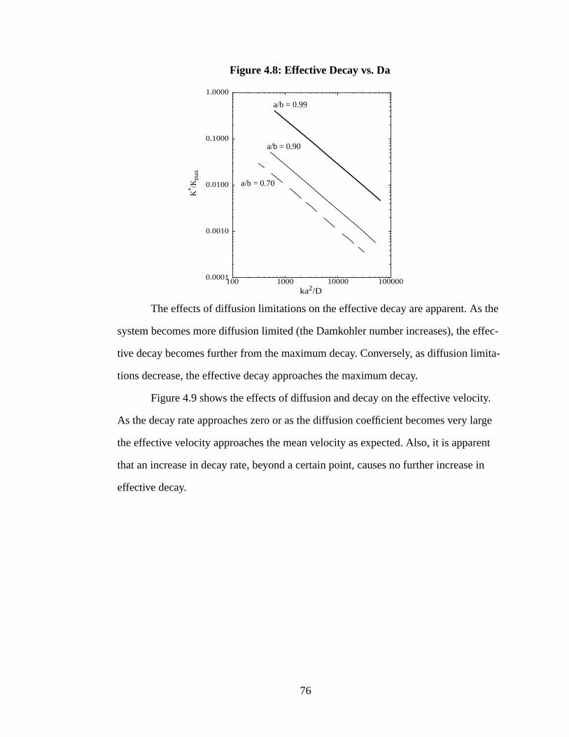
Figure 4.8: Effective Decay vs. Da

The effects of diffusion limitations on the effective decay are apparent. As the

system becomes more diffusion limited (the Damkohler number increases), the effec-

tive decay becomes further from the maximum decay. Conversely, as diffusion limita-

tions decrease, the effective decay approaches the maximum decay.

Figure 4.9 shows the effects of diffusion and decay on the effective velocity.

As the decay rate approaches zero or as the diffusion coefficient becomes very large

the effective velocity approaches the mean velocity as expected. Also, it is apparent

that an increase in decay rate, beyond a certain point, causes no further increase in

effective decay.

100 1000 10000 100000ka2/D

0.0001

0.0010

0.0100

0.1000

1.0000

K* /K

max

a/b = 0.99

a/b = 0.90

a/b = 0.70

76

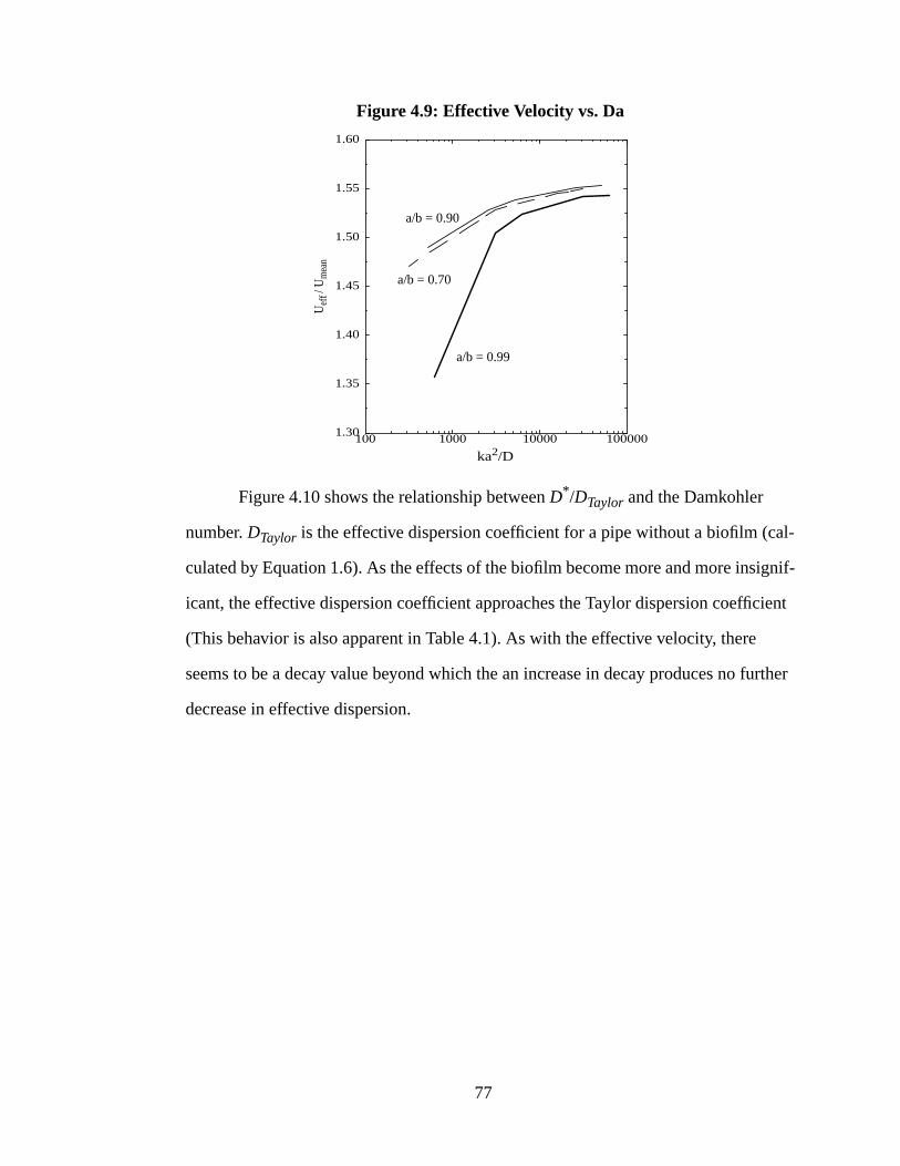
Figure 4.9: Effective Velocity vs. Da

Figure 4.10 shows the relationship between D*/DTaylor and the Damkohler

number. DTaylor is the effective dispersion coefficient for a pipe without a biofilm (cal-

culated by Equation 1.6). As the effects of the biofilm become more and more insignif-

icant, the effective dispersion coefficient approaches the Taylor dispersion coefficient

(This behavior is also apparent in Table 4.1). As with the effective velocity, there

seems to be a decay value beyond which the an increase in decay produces no further

decrease in effective dispersion.

100 1000 10000 100000

ka2/D

1.30

1.35

1.40

1.45

1.50

1.55

1.60

Uef

f / U

mea

n

a/b = 0.99

a/b = 0.70

a/b = 0.90

77

Figure 4.10: Effective Dispersion vs. Da

4.2 Turbulent Flow Results for a Smooth Pipe

The turbulent flow models generate the same output as the laminar flow mod-

els. Zeroth, first, and second mass moment curves are used to determine the effective

transport parameters through regression analysis. Since there is considerable interest

in turbulent pipe flow systems with no reactive biofilm, simulations were performed to

characterize transport in turbulent flow with and without a boundary reaction.

Turbulent Transport With No Boundary Reaction

A set of simulations were used to compare the particle tracking results with

Taylor’s 1954 turbulent flow results. The analytical solution, discussed in Chapter 3, is

used to verify the particle tracking model. The following simulations, shown in

Table 4.11, were performed with a pipe radius of 4.0 cm and a molecular diffusion

coefficient of 1.0x10-5 cm2/s. The Reynolds number was varied to show its effect on

the effective longitudinal dispersion coefficient.

100 1000 10000 100000

ka2/D

0.1

1.0

D* /

DTa

ylor

a/b = 0.99

a/b = 0.90

a/b = 0.70

78

The effect of Reynolds number on the asymptotic longitudinal dispersion coef-

ficient is apparent. At lower Reynolds numbers, the laminar sublayer is considerably

thicker. Therefore, more solute mass can become trapped in the sublayer and separated

from the mass in the turbulent core. As the Reynolds number increases, however, the

laminar sublayer becomes extremely thin and is unable to hold a considerable amount

of mass. Therefore the laminar sublayer, and changes in the Reynolds number itself,

will have very little impact on the effective dispersion coefficient at high Reynolds

numbers.

It is obvious that Taylor’s result, D* = 10.1au*, does not apply for the velocity

and diffusivity distributions used in this research. The velocity profile, and hence the

diffusivity profile, used by Taylor does not vary with Reynolds number. Therefore, his

analysis results in a constant, 10.1, multiplied by au*. The velocity profile used in the

particle tracking and analytical models does vary with Reynolds number, hence the

discrepancy with Taylor’s result is expected. In the field of Civil Engineering, no stud-

ies have been performed to verify Taylor’s result (since Taylor’s experimentation in

1954). However, there has been considerable research attempting to develop expres-

sions for velocity and diffusivity in the wall region. The velocity and diffusivity pro-

files used in this research (Wasan and Wilke, 1964), are accepted as a more accurate

description of transport in the wall region than Taylor’s. It is then reasonable to assume

Table 4.11: Effect of Reynolds Number on Effective Dispersion

Reynolds NumberEffective Dispersion(Particle Tracking)

Effective Dispersion(Analytical Solution)

10000 29.3au* 29.3au*

50000 8.1au* 8.0au*

100000 6.5au* 6.1au*

500000 5.7au* 5.3au*

1000000 5.3au* 5.1au*

79

that the results given by the particle tracking model provide a better representation of

dispersion in turbulent pipe flow than Taylor’s result. However, experimental results

are required to confirm this hypothesis.

Taylor’s experimental results vary from 10.6au* to 12.8au*. These experiments

were run for Reynolds numbers near 20000 without much variation. The particle

tracking model gives a value of approximately 14au* for a Reynolds number of 20000.

The model results therefore seem to overprotect the dispersion seen in Taylor’s experi-

ments. It is possible that the velocity profile used in Taylor’s analysis was developed

from the profile seen in the experiments. This would explain the close correlation

between the theory and experimentation. Since the Reynolds number was not varied

greatly, the relationship between Reynolds number and effective dispersion went

unnoticed. However, before any final conclusions can be reached on this issue, addi-

tional physical experimentation should be performed for a wide range of Reynolds

numbers.

Turbulent Transport with a Reactive Biofilm

Once the turbulent flow model was verified analytically for the non-reactive

case, it was extended to include a boundary reaction. No analytical solutions are avail-

able for this system so there is currently no way to verify these results. Physical exper-

imentation is necessary in order to ensure that the model is working properly.

Four simulations were run to show the effects of a reactive biofilm and to com-

pare the results to a similar system with no biofilm and a system with a non-reactive

biofilm. The simulations were run with at a Reynolds number of 100,000, a pipe radius

b of 5.0 cm, a biofilm thickness of 0.3 cm (a = 4.7), a first order decay constant of -

15.0 s-1, porosity of 0.73, and D/Db of 0.6. This results in a mean flow velocity of

104.3 cm/s and a shear velocity of 4.94 cm/s. The required timestep for this system is

0.0001 seconds and 50,000 particles were used in the simulation. The total observation

80

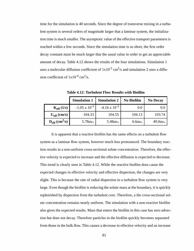
time for the simulation is 40 seconds. Since the degree of transverse mixing in a turbu-

lent system is several orders of magnitude larger that a laminar system, the initializa-

tion time is much smaller. The asymptotic value of the effective transport parameters is

reached within a few seconds. Since the simulation time is so short, the first order

decay constant must be much larger that the usual value in order to get an appreciable

amount of decay. Table 4.12 shows the results of the four simulations. Simulation 1

uses a molecular diffusion coefficient of 1x10-5 cm2/s and simulation 2 uses a diffu-

sion coefficient of 1x10-4 cm2/s.

It is apparent that a reactive biofilm has the same effects on a turbulent flow

system as a laminar flow system, however much less pronounced. The boundary reac-

tion results in a non-uniform cross-sectional solute concentration. Therefore, the effec-

tive velocity is expected to increase and the effective diffusion is expected to decrease.

This trend is clearly seen in Table 4.12. While the reactive biofilm does cause the

expected changes in effective velocity and effective dispersion, the changes are very

slight. This is because the rate of radial dispersion in a turbulent flow system is very

large. Even though the biofilm is reducing the solute mass at the boundary, it is quickly

replenished by dispersion from the turbulent core. Therefore, a the cross-sectional sol-

ute concentration remains nearly uniform. The simulation with a non-reactive biofilm

also gives the expected results. Mass that enters the biofilm in this case has zero advec-

tion but does not decay. Therefore particles in the biofilm quickly becomes separated

from those in the bulk flow. This causes a decrease in effective velocity and an increase

Table 4.12: Turbulent Flow Results with Biofilm

Simulation 1 Simulation 2 No Biofilm No Decay

Keff (1/s) -1.05 x 10-3 -4.16 x 10-3 0.0 0.0

Ueff (cm/s) 104.33 104.55 104.13 103.74

Deff (cm2/s) 5.78au* 5.48au* 6.6au* 49.0au*

81

in effective dispersion.

The differences between Simulation 1 and Simulation 2 are due to the differ-

ence in the molecular diffusion coefficient. A change in molecular diffusion of one

order of magnitude only produces slight changes in the effective transport parameters.

It is then obvious that the role of the molecular diffusion coefficient in a turbulent flow

system is much different from its role in a laminar flow system. In a laminar flow field,

transport in the radial direction occurs as a result of molecular diffusion only. How-

ever, in a turbulent system, radial transport is governed by the turbulent eddies existing

within the flow field. Recall from Chapter 2 that the radial dispersion is a function of

the slope of the velocity profile, which is several orders of magnitude larger than the

molecular diffusion coefficient. Only in the laminar sublayer, very close to the biofilm,

does the molecular diffusion coefficient have an impact. Even so, the effects of molec-

ular diffusion are obvious. The laminar sublayer controls the transport of solute into

the biofilm. As the molecular diffusion increases, more solute will enter the biofilm.

Therefore, the effective decay rate should increase. As decay increases the amount of

mass located in the region of lowest velocity and highest shear (near the boundary)

decreases. This causes an increase in the effective velocity and a decrease in effective

dispersion. These trends are clearly seen in Table 4.12.

Reynolds Number Dependence

Table 4.13 shows the effects of Reynolds number on the effective transport

parameters. The apparent trends are the result of changes in the laminar sublayer thick-

ness. As the Reynolds number increases the laminar sublayer thickness decreases.

Therefore, the rate of diffusion into the biofilm increases. This results in an increase in

the effective decay coefficient. As the laminar sublayer thickness decreases, radial

transport in the wall region of the pipe increases. Therefore, a more uniform concen-

tration distribution is maintained throughout the pipe cross section and the effective

82

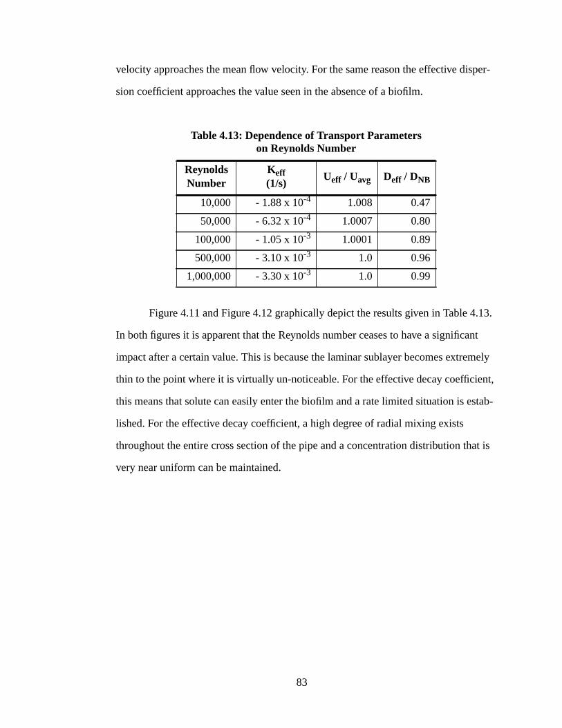
velocity approaches the mean flow velocity. For the same reason the effective disper-

sion coefficient approaches the value seen in the absence of a biofilm.

Figure 4.11 and Figure 4.12 graphically depict the results given in Table 4.13.

In both figures it is apparent that the Reynolds number ceases to have a significant

impact after a certain value. This is because the laminar sublayer becomes extremely

thin to the point where it is virtually un-noticeable. For the effective decay coefficient,

this means that solute can easily enter the biofilm and a rate limited situation is estab-

lished. For the effective decay coefficient, a high degree of radial mixing exists

throughout the entire cross section of the pipe and a concentration distribution that is

very near uniform can be maintained.

Table 4.13: Dependence of Transport Parameterson Reynolds Number

Reynolds Number

Keff(1/s)

Ueff / Uavg Deff / DNB

10,000 - 1.88 x 10-4 1.008 0.47

50,000 - 6.32 x 10-4 1.0007 0.80

100,000 - 1.05 x 10-3 1.0001 0.89

500,000 - 3.10 x 10-3 1.0 0.96

1,000,000 - 3.30 x 10-3 1.0 0.99

83

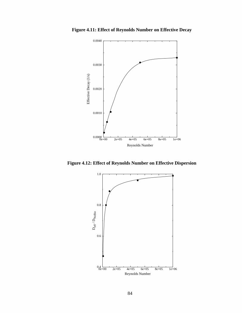
Figure 4.11: Effect of Reynolds Number on Effective Decay

Figure 4.12: Effect of Reynolds Number on Effective Dispersion

0e+00 2e+05 4e+05 6e+05 8e+05 1e+06

Reynolds Number

0.0000

0.0010

0.0020

0.0030

0.0040

Eff

ectiv

e D

ecay

(1/

s)

0e+00 2e+05 4e+05 6e+05 8e+05 1e+06

Reynolds Number

0.4

0.6

0.8

1.0

Def

f / D

NoB

io

84

Sensitivity to Damkohler Number

As with the laminar flow model, the effects of diffusion limitations on the tur-

bulent flow effective parameters are examined through the dimensionless Damkohler

number. For turbulent flow, the Damkohler number is computed as ka2/D where D is

the average value of the radial dispersion coefficient.

Figure 4.13 shows the relationship between the Damkohler number and effec-

tive decay for two ratios a/b and for two different Reynolds numbers. At low

Damkohler numbers the system is rate limited and the effective decay approaches the

maximum decay seen in the absence of diffusion limitations. At high Damkohler num-

bers the system is more diffusion limited and the effective decay is much smaller than

the maximum decay. These results are almost identical to those seen in the laminar

flow case (Figure 4.8).

Figure 4.13: Effective Decay vs. Damkohler Number

The influence of the Damkohler number on effective velocity is not shown

because the variations in effective velocity are too small to display in a graphically

1 10 100 1000

ka2/D

0.0001

0.0010

0.0100

0.1000

1.0000

Kef

f / K

max

a/b = 0.99

a/b = 0.90

- - - Re = 100,000

Re = 50,000

85

meaningful way. In turbulent flow, the effective velocity is always very close to the

mean flow velocity (differences on the order of 10-2 - 10-3).

Figure 4.14 shows the relationship between the Damkohler number and the

effective dispersion coefficient. The figure shows the results for two different Reynolds

numbers for an a/b ratio of 0.9. Only one a/b ratio is displayed because the results for

different ratios are almost identical. The general trend shown in the figure is similar to

that seen in the laminar flow case (Figure 4.10). In a rate limited scenario (low

Damkohler number), the concentration distribution is nearly uniform, so the effective

dispersion approaches and actually exceeds the dispersion value for the no biofilm

case. The reason that the effective dispersion value exceeds DNoBio is due to a storage

effect in the biofilm. At low Damkohler numbers, mass is entering the biofilm but it is

not decaying very fast. Therefore, mass is stored in the biofilm and is quickly sepa-

rated from mass in the bulk flow. In a diffusion limited scenario, less mass exists near

the pipe wall where the shear is greatest. Therefore, there is less longitudinal separa-

tion of particles and the effective dispersion coefficient decreases from the dispersion

seen in the absence of a biofilm.

86

Figure 4.14: Effective Dispersion vs. Damkohler Number

1 10 100 1000

ka2/D

0.80

1.00

1.20

1.40

1.60

Def

f / D

NoB

io

- - - Re = 100,000

Re = 50,000

87

Chapter 5

Conclusion

A particle tracking model was used to quantify the effective transport parame-

ters in a circular pipe with a reactive biofilm. First order kinetics were used to model

decay in the biofilm region. Solute transport under laminar flow conditions was exam-

ined and verified with the analytical solutions developed by Cox (1997). A turbulent

flow model was used to examine solute transport with and without the effects of a

reactive biofilm. For the case of turbulent flow without a biofilm, the effective disper-

sion coefficient was compared with Taylor’s result of 10.1au*. Using more recently

accepted velocity profiles in the turbulent core and the wall region, it becomes appar-

ent that Taylor’s result is not valid for a range of Reynolds numbers.

Under laminar flow conditions, the model results provide considerable insight

into the relationship between biofilm characteristics and the effective bulk flow param-

eters. It is shown that a reactive biofilm results in a non-uniform distribution of solute

across the pipe cross section. Since less solute mass exists near the pipe wall, the effec-

tive velocity is greater than the mean velocity and the effective dispersion is less than

the dispersion in a pipe with no biofilm. A sensitivity analysis to porosity and D/Db

shows that the model is not very sensitive to changes in these two parameters. How-

ever, the sensitivity is greater in rate limited systems than in diffusion limited systems.

In general, as the reactive potential in the biofilm increase, whether through an

increased decay rate, increased porosity, or biofilm thickness, the effective decay and

velocity tend to increase and the effective dispersion tends to decrease.

For comparison with the Horn and Hempel experiments, simulations were per-

formed for a wide range of Reynolds numbers. Contrary to the Horn and Hempel

results, the effective decay coefficient does not depend on the Reynolds number. It is

apparent that the Horn and Hempel experiments are observing pre-development effec-

tive decay coefficients. Therefore, their expression for the mass transfer coefficient

does not represent the asymptotic effective decay rate that may be used in an effective

one-dimensional advection-diffusion reaction equation.

The development of the turbulent flow models required research into the nature

of the velocity profile and eddy diffusivity in the wall region of the pipe. The well-

known universal velocity profile was used in the turbulent core. In the laminar sub-

layer, expressions developed by Wasan, Wilke, and Tien (1963) were used to describe

the velocity and eddy diffusivity. Using these profiles, a particle tracking model was

constructed to determine the effective dispersion coefficient for a pipe with no biofilm.

The results were verified by an analytical solution based on Taylor’s analysis and were

compared to his expression of 10.1au* for the effective dispersion coefficient. Since

the velocity profiles used in the particle tracking model varied with Reynolds number,

the resulting effective dispersion coefficient should also with Reynolds number. This

relationship was clearly seen in the model results and the “constant” 10.1 was actually

much higher for low Reynolds number and was lower for high Reynolds numbers.

Taylor’s analysis, however, was based on a velocity profile which did not change with

Reynolds number. Hence, his analysis was unable to capture the effects of changes in

the laminar sublayer thickness at different Reynolds numbers. Since the physical

experiments used to verify Taylor’s analysis did not include a wide range of Reynolds

numbers, this behavior went unnoticed. It is probable that the velocity profile used in

Taylor’s result was developed from velocity data seen in the pipe experiments (or from

89

an experiment performed at similar Reynolds numbers). Therefore, this topic should

be re-examined with additional physical experimentation for a wide range of Reynolds

numbers.

Simulations were also performed to analyze the influence of a reactive biofilm

on the effective transport parameters in a turbulent flow field. Since no previous

research has been done in this area, and no analytical solutions to this problem exist,

the particle tracking results could not be verified. Similar trends between the biofilm

parameters and the bulk transport parameters were seen in the turbulent flow model

and the laminar flow model. The presence of a reactive biofilm results in a non-uni-

form, cross sectional concentration distribution. Therefore, the effective velocity

increases from the mean velocity and the effective dispersion decreases from the dis-

persion in a pipe with no biofilm. The variations in the effective parameters, however,

are much less pronounced in the turbulent flow model than in the laminar flow model.

Since there is considerable lateral mixing due to turbulent eddies, a cross sectional

concentration distribution that is very near uniform is always maintained. Therefore,

the biofilm only affects a very small region of flow near the pipe wall (namely the lam-

inar sublayer). As the Reynolds number increases, the thickness of this region

decreases and the effects of the biofilm become less significant. For this reason, and

unlike the laminar flow system, the effective decay rate in a turbulent flow system var-

ies with Reynolds number.

90

References

(Aris, 1956)Aris, R. 1956. On the Dispersion of a Solute in a Fluid Flowing

Through a Tube. Proc. R. Soc. London Ser. A 235.

(Chapra, 1997)Chapra, Steven C. 1997. Surface Water-Quality Modeling. The

McGraw-Hill Companies Inc., United States of America.

(Cox, 1997)Cox, T.J. 1997. Investigation and Quantification of Boundary Reaction

Effect on Solute Transport Parameterization. University of Colorado at Boul-der. Boulder, Colorado.

(Fischer, 1979)Fischer, H.B., et.al. 1979. Mixing in Inland and Coastal Waters. Aca-

demic Press Inc., Boston, MA.

(Horn and Hempel, 1995)Horn, H., Hempel, D.C. 1995. Mass Transfer Coefficients for an

Autotrophic and a heterotrophic Biofilm System. Water Science Technology. Vol. 32. No. 8. pp 199-204.

(Li and Chen, 1994)Li, S., Chen, G.H. 1994. Modeling the Organic Removal and Oxygen

Consumption by Biofilms in an Open-Channel Flow. Water Science Technol-ogy. Vol. 30. No. 2. pp 53-61.

(Taylor, 1953)Taylor, G.I. 1953. Dispersion of Soluable Matter in Solvent Flowing

Slowly Through a Tube. Proc. R. Soc. London Ser. A 219.

(Taylor, 1954)Taylor, G.I. 1954. The Dispersion of Matter in Turbulent Flow Through

a Pipe. Proc. R. Soc. London Ser. A 223.

(Tompson, 1988)Tompson, Andrew, et.al. 1988. Numerical Simulation of Solute Trans-

port in Randomly Heterogeneous Porous Media: Motivation, Model Develp-ment, and Application. Department of Civil Engineering. Massachusetts Institute of Technology. Cambridge, Massachusetts.

(Wasan and Tien, 1963)Wasan, D.T., Tien, C.L., and Wilke, C.R. 1963. Theoretical Correlation

of Velocity and Eddy Viscosity for Flow Close to a Pipe Wall. A.I.Ch.E. Jour-nal.

(Wasan and Wilke, 1964)Wasan, D.T. and Wilke, C.R. 1964. Turbulent Exchange of Momentum,

Mass, and Heat Between Fluid Streams and Pipe Wall. Int. J. Heat Mass Trans-fer, Vol. 7, pp. 87-94.

(Wilkes, 1999)Wilkes, J.O. 1999. Fluid Mechanics for Chemical Engineers. Prentice-

Hall, Inc., Upper Saddle River, New Jersey.

(Zhang and Bishop 1, 1994)Zhang, Tian C., and Bishop, Paul L. 1994. Density, Porosity, and Pore

Structure of Biofilms. Water Research. Vol. 28. No. 11. pp 2267-2278.

(Zhang and Bishop 2, 1994)Zhang, Tian C., and Bishop, Paul L. 1994. Evaluation of Tortuosity

Factors and Effective Diffusivities in Biofilms. Water Research. Vol. 28. No. 11. pp 2279-2287.

92