NASA/CR–2011-216413

Investigating the Nature of and Methods for Managing Metroplex OperationsStephen Atkins, Brian Capozzi, and Jim HinkeyMosaic ATM, Inc.Leesburg, Virginia

Husni IdrisEngility CorporationBillerica, Massachusetts

Kent KaiserMosaic ATM, Inc.Leesburg, Virginia

June 2011

https://ntrs.nasa.gov/search.jsp?R=20110023767 2018-06-16T12:30:05+00:00Z

Since its founding, NASA has been dedicated to the advancement of aeronautics and space science. The NASA Scientific and Technical Information (STI) Program Office plays a key part in helping NASA maintain this important role.

The NASA STI Program Office is operated by Langley Research Center, the Lead Center for NASA’s scientific and technical information. The NASA STI Program Office provides access to the NASA STI Database, the largest collection of aeronautical and space science STI in the world. The Program Office is also NASA’s institutional mechanism for disseminating the results of its research and development activities. These results are published by NASA in the NASA STI Report Series, which includes the following report types:

• TECHNICAL PUBLICATION. Reports of completed research or a major significant phase of research that present the results of NASA programs and include extensive data or theoreti‑cal analysis. Includes compilations of significant scientific and technical data and information deemed to be of continuing reference value. NASA’s counterpart of peer‑reviewed formal professional papers but has less stringent limita‑tions on manuscript length and extent of graphic presentations.

• TECHNICAL MEMORANDUM. Scientific and technical findings that are preliminary or of specialized interest, e.g., quick release reports, working papers, and bibliographies that contain minimal annotation. Does not contain extensive analysis.

• CONTRACTOR REPORT. Scientific and techni‑cal findings by NASA‑sponsored contractors and grantees.

The NASA STI Program Office . . . in Profile

• CONFERENCE PUBLICATION. Collected papers from scientific and technical confer‑ences, symposia, seminars, or other meetings sponsored or cosponsored by NASA.

• SPECIAL PUBLICATION. Scientific, technical, or historical information from NASA programs, projects, and missions, often concerned with subjects having substantial public interest.

• TECHNICAL TRANSLATION. English‑ language translations of foreign scientific and technical material pertinent to NASA’s mission.

Specialized services that complement the STI Program Office’s diverse offerings include creating custom thesauri, building customized databases, organizing and publishing research results . . . even providing videos.

For more information about the NASA STI Program Office, see the following:

• Access the NASA STI Program Home Page at http://www.sti.nasa.gov

• E‑mail your question via the Internet to help@sti.nasa.gov

• Fax your question to the NASA Access Help Desk at (301) 621‑0134

• Telephone the NASA Access Help Desk at (301) 621‑0390

• Write to: NASA Access Help Desk NASA Center for AeroSpace Information 7115 Standard Drive Hanover, MD 21076‑1320

NASA/CR–2011-216413

Investigating the Nature of and Methods for Managing Metroplex OperationsStephen Atkins, Brian Capozzi, and Jim HinkeyMosaic ATM, Inc.Leesburg, Virginia

Husni IdrisEngility CorporationBillerica, Massachusetts

Kent KaiserMosaic ATM, Inc.Leesburg, Virginia

June 2011

National Aeronautics andSpace Administration

Ames Research CenterMoffett Field, California 94035‑1000

Available from:

NASA Center for AeroSpace Information National Technical Information Service7115 Standard Drive 5285 Port Royal RoadHanover, MD 21076‑1320 Springfield, VA 22161(301) 621‑0390 (703) 487‑4650

iii

TABLE OF CONTENTS

LIST OF FIGURES ...................................................................................................................... vii

LIST OF TABLES ......................................................................................................................... xi

ACRONYMS ............................................................................................................................... xiii

1 INTRODUCTION .....................................................................................................................1 1.1 Motivation and Objectives ................................................................................................1 1.2 Scope and Report Organization ........................................................................................1 1.3 Publications .......................................................................................................................2

2 METROPLEX OBSERVATIONS ............................................................................................3 2.1 Literature Survey ..............................................................................................................3 2.2 Site Visits ..........................................................................................................................3 2.3 San Francisco Bay Area Metroplex ..................................................................................4 2.4 Generalized Metroplex Observations ...............................................................................4 2.5 Generalized Metroplex Management Approaches ............................................................7

3 METROPLEX DEFINITION ....................................................................................................9

3.1 Qualitative Metroplex Definition ......................................................................................9 3.2 Types of Quantitative Definitions ...................................................................................10

4 METROPLEX MODELING ...................................................................................................11

4.1 Modeling Current Metroplex Costs ................................................................................11 4.2 Part-Metroplex Models ...................................................................................................12 4.3 Metroplex Simulation Environment ...............................................................................14 4.4 TRAC ..............................................................................................................................16

5 METROPLEX TRAFFIC MANAGEMENT DECOMPOSITION .........................................17

5.1 Space of NextGen Approaches .......................................................................................17 5.2 Spatial and Temporal Metroplex Management Concepts. ..............................................18 5.3 Problem Decomposition..................................................................................................20

6 METROPLEX PLANNER INTRODUCTION .......................................................................22 7 FORMULATION AS A MIXED-INTEGER LINEAR PROGRAM .....................................25

7.1 Preliminaries and Notation .............................................................................................25 7.2 Decision Variables ..........................................................................................................28 7.3 Notions of Time ..............................................................................................................28 7.4 Objective Function ..........................................................................................................29 7.5 Constraints ......................................................................................................................29 7.6 Transformation to Linear Form ......................................................................................32 7.7 Heuristics to Reduce Computation Time ........................................................................36

iv

TABLE OF CONTENTS (cont.)

8 MODELING CONSTRAINT PARAMETERS ......................................................................38 8.1 Computing Earliest Time at Initial Scheduling Point .....................................................39 8.2 Estimating Fast and Slow Transit Times between Schedule Points ...............................40 8.3 Establishing Required Separation between Flights at Schedule Points ..........................46

9 DYNAMIC PLANNING APPLICATIONS ...........................................................................49

9.1 Architecture .....................................................................................................................49 9.2 Interfaces between Simulation and Planner ....................................................................50 9.3 Overview of Processing Flow .........................................................................................52 9.4 Control of Time...............................................................................................................53 9.5 Plan Stability: Freeze Horizons ......................................................................................55 9.6 Simple Dynamic Planning Examples..............................................................................56

10 SUMMARY AND LESSONS LEARNED .............................................................................63

10.1 Summary of Accomplishments .......................................................................................63 10.2 Lessons Learned and Next Steps ....................................................................................64

11 NUMERICAL RESULTS .......................................................................................................65

11.1 Analysis of Scalability ....................................................................................................65 11.2 Comparison against Greedy FCFS Planner ....................................................................75

12 DYNAMIC PLANNING DEPLOYMENT .............................................................................82

12.1 System Requirements and Configuration .......................................................................82 12.2 Application Configuration ..............................................................................................82 12.3 Running the Dynamic Planning Application ..................................................................86 12.4 Dynamic Planning Verification ......................................................................................87

13 ORGANIZING METROPLEX TRAFFIC BASED ON SPEED SEGREGATION AND

TRAJECTORY FLEXIBILITY ...............................................................................................93 13.1 Introduction .....................................................................................................................93 13.2 Metroplex Inefficiencies and Proposed Solutions ..........................................................94 13.3 Analysis Approach and Design .......................................................................................96 13.4 Simulation Results and Observations .............................................................................99 13.5 Conclusions ...................................................................................................................107

14 AIRCRAFT MODELS ..........................................................................................................107

14.1 Aircraft Dynamics Model .............................................................................................108 14.2 Guidance Model ............................................................................................................113 14.3 A More Suitable Approach to Modeling .....................................................................119

v

TABLE OF CONTENTS (cont.)

15 CONCLUSIONS....................................................................................................................123 15.1 Summary .......................................................................................................................123 15.2 Future Work ..................................................................................................................124

16 REFERENCES ......................................................................................................................125

vi

vii

LIST OF FIGURES

Figure 1. Airports and runway orientation for San Francisco Bay Area metroplex airports. .......5

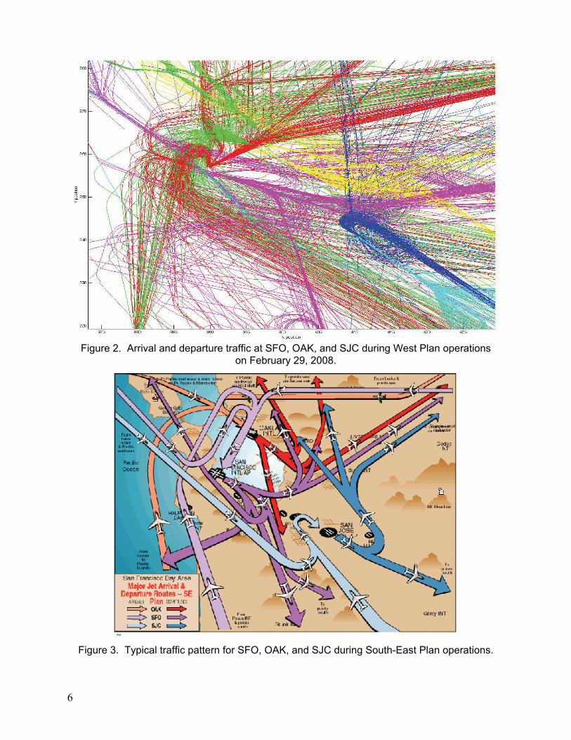
Figure 2. Arrival and departure traffic at SFO, OAK, and SJC during West Plan operations on February 29, 2008. ....................................................................................................6

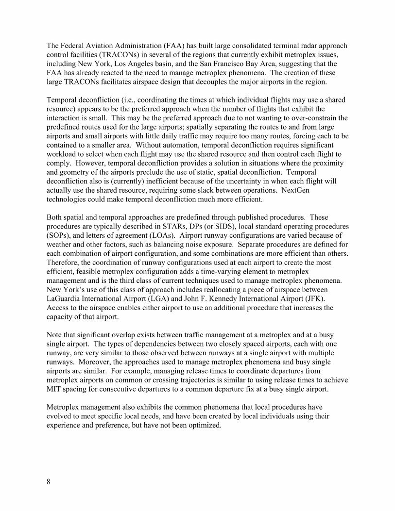
Figure 3. Typical traffic pattern for SFO, OAK, and SJC during South-East Plan operations. ....6

Figure 4. Overview diagram of MATLAB model. .....................................................................13

Figure 5. Example results from a two-airport case with uncertain flight time and control applied both at the runways and in the air. ..................................................................13

Figure 6. Potential conflicts by pairs of flows and horizontal and vertical thresholds. ..............14

Figure 7. Notional diagram of the metroplex simulation environment. ......................................15

Figure 8. Example of actual trajectories displayed and “backbone” routes defined using TRAC. ..........................................................................................................................16

Figure 9. SFO and OAK West Plan arrival and departure routes defined using TRAC. ............17

Figure 10. Spatial versus temporal approaches. ............................................................................20

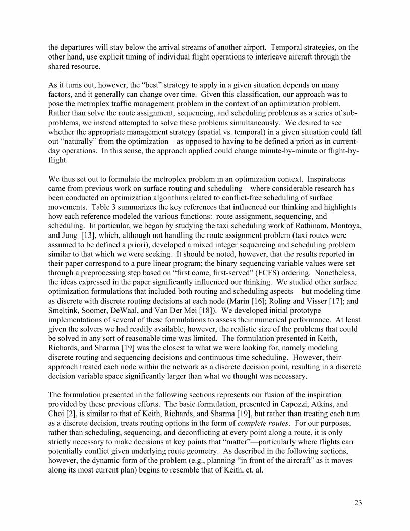
Figure 11. Notional metroplex boundary showing flights in various states. .................................26

Figure 12. Notional routing structure connecting metroplex entry and exit points. .....................26

Figure 13. Effective routing structure changes include only options in front of aircraft, and enforce constraints only at potentially shared points (shown in red). ...................28

Figure 14. Graphical depiction of earliest initial scheduling constraint and transit variations. ....30

Figure 15. Routes used for highlighting the effect of no-pass constraints. ...................................36

Figure 16. Variable substitutions to be made for all pairs of flights that can be routed on R1 or R2. ......................................................................................................................37

Figure 17. Variable substitutions to be made for each pair of flights routed on R1. ....................37

Figure 18. Strategies for changing speed to attain target airspeeds above or below the current airspeed. ...........................................................................................................40

Figure 19. Notional path control options for adjusting transit time between SP1 and SP2. .........41

Figure 20. Representative speed profile specification along a route. ............................................42

Figure 21. Relationship between different time concepts for a flight. ..........................................47

Figure 22. Overlap in distribution of crossing times for two flights. ...........................................47

Figure 23. Option 1 – Delay trailing flight such that ETAs satisfy minimum separation. ...........47

Figure 24. Buffering applied to nominal separation to account for “late” leader and “early” follower. .......................................................................................................................48

Figure 25. High-level architecture of dynamic planning simulation environment. ......................49

Figure 26. Simple uncertainty model provided by default implementation. ................................52

Figure 27. Key timing relationships used in dynamic planning simulation framework. ..............54

Figure 28. Abstract depiction of freeze horizon—selective data from previous plan is frozen and used as constraints in developing the current plan. ....................................55

viii

LIST OF FIGURES (CONT.)

Figure 29. Examples of application of freeze horizon at different points. ...................................56 Figure 30. Simple arrival scenario. ...............................................................................................57 Figure 31. Representative time-of-arrival graphic at the fix E1. ..................................................58 Figure 32. Relative position of arrival flights just before FA1 crosses the arrival fix E1. ...........59 Figure 33. Variation in actual speed of aircraft within simulation over time. ..............................59 Figure 34. Time-of-arrival plot for FD1 and FD2 approach fix N1. ............................................62 Figure 35. Actual speeds of flight FD2 within the simulation as it moves along its route. ..........62 Figure 36. Summary of key optimization-based planner development milestones. .....................64 Figure 37. Route structure for single-route case. ..........................................................................66 Figure 38. Variation in simplex solver time as a function of the number of flights in the

demand set for the single-route problem consisting of three schedule points. ............67 Figure 39. Effect of no-pass constraint and FCFS heuristic on number of binary variables

needed to model a problem with N flights. ..................................................................67 Figure 40. Log(10) plot of variation in solver time as function of the number of flights in

the demand set. .............................................................................................................68 Figure 41. Route structure for two-independent-routes case. .......................................................69 Figure 42. Variation of solution time with demand size for two-independent-routes case. ..........70 Figure 43. Effect of various heuristics in reducing the number of binary variables. ....................70 Figure 44. Variation of solver time with number of flights—presented on log(10) scale. ...........71 Figure 45. Route structure for two-merging-routes case. ..............................................................71 Figure 46. Variation in solver time with number of flights in demand set for two-merging-

routes example. ............................................................................................................72 Figure 47. Zooming in on variation of solver time with size of demand set for two merging

routes. ..........................................................................................................................72 Figure 48. Effect of various heuristics on number of binary variables for two merging routes. ..73 Figure 49. Variation in log(10) (solver time) with size of demand set for two merging routes

under different solver heuristic configurations. ...........................................................73 Figure 50. Comparison of greedy FCFS (blue circles) and MILP solution (red asterisks) for

alternating types. ..........................................................................................................76 Figure 51. Distribution of delay comparison for alternative types example problem. ..................77 Figure 52. Route structure used for shared-departure-fix example scenario. ................................78

Figure 53. Variation in STA at the fix for both greedy FCFS (in blue) and MILP (in red) planners. Flights over fixes E1 and E2 are represented by circles and asterisks, respectively. .................................................................................................................79

Figure 54. Resource timing view comparing STA and fix selection made by greedy FCFS and MILP planners for shared-departure-fix case. ......................................................80

Figure 55. Resourcing timing plot for shared-departure-fix equidistant-from-runways case. ......80

ix

LIST OF FIGURES (CONT.)

Figure 56. Resourcing timing plot comparison for the shared-departure-fix case by the greedy FCFS and MILP planners when their objective functions are matched. .........81

Figure 57. Depiction of flight FA1 approaching runway SFO28R and flight FD1 approaching schedule point DP1. ................................................................................90

Figure 58. Comparison of various times of arrival. ......................................................................91 Figure 59. Close-up comparison figure of times of arrival for flights FA1 and FA2. ..................91 Figure 60. Example of metroplex interdependency. .....................................................................95 Figure 61. Segregation by speed instead of by destination airport. ..............................................96 Figure 62. Using blocked polygons to establish a trombone pattern. ...........................................98 Figure 63. Two single-airport scenario cases. ..............................................................................99 Figure 64. Throughput analysis in single-airport scenario. ........................................................101 Figure 65. Trajectory flexibility analysis in single-airport scenario. ..........................................102 Figure 66. Two two-airport scenario cases. ................................................................................103 Figure 67. Throughput analysis in two-airport scenario. ............................................................104 Figure 68. Trajectory flexibility analysis in two-airport scenario. .............................................106 Figure 69. Simulink representation of rudimentary autopilot for point mass model

of GA aircraft. ............................................................................................................112 Figure 70. Diagram for guidance-law development. ..................................................................113 Figure 71. Integrated guidance with the autopilot and aircraft. ..................................................114 Figure 72. Desired altitude as a function of the x- and y-position of the vehicle. ......................115 Figure 73. Distance metric used in calculation of time of arrival. ..............................................116 Figure 74. Simple example where a desired final velocity can be reached at a specified

RTA, given the application of a single constant deceleration. ..................................117 Figure 75. Example trajectory ground track. ..............................................................................118 Figure 76. Example trajectory descent profile. ...........................................................................118 Figure 77. Additional state histories from the guidance and control simulation example. ........119

Figure 78. Free-body diagram of aircraft in equilibrium. ...........................................................120 Figure 79. Analytical results can be calculated on a discrete per-segment basis. ......................121

x

xi

LIST OF TABLES

Table 1. Modeled SFO-OAK Silent/Quiet Delays .....................................................................12 Table 2. Space of NextGen Metroplex Management Approaches .............................................18 Table 3. Summary of Key References That Shaped the MILP Formulation Developed in

This Research ...............................................................................................................24 Table 4. Variation in Transit Time between Points A and B Achievable via Different

Speed Strategies ...........................................................................................................44 Table 5. Summary of Route Geometry, Speed Profile, and Transit-Time Bounds for

Simple Departure Scenario ..........................................................................................60 Table 6. Evolution of STAs across Planning Cycles for FD2 at Various Points Along

Its Route .......................................................................................................................61 Table 7. Comparison of Solvers for Single-Route Example—Variation with Number

of Flights ......................................................................................................................69 Table 8. Effect of Adding Initial Time Penalty on Solution Time and Solution Obtained

for Single-Route Case ..................................................................................................74 Table 9. Effect of Adding Penalty on Time at Initial Scheduling Point on Solution Time

for Two Independent Routes ........................................................................................74 Table 10. Effect of Penalty on Time at Initial Scheduling Point on Solution Time for the

Two-Merging-Routes Case ..........................................................................................75 Table 11. Constraints Considered by the Planner ........................................................................83

xii

xiii

ACRONYMS

A90 Boston Consolidated TRACON, Boston, Massachusetts

AOA angle of attack

AR aspect ratio

ARTCC Air Route Traffic Control Centers

ASP Airspace Systems Program

ATA actual time of arrival

ATC air traffic control

BADA base of aircraft data

CDA Continuous Descent Approaches

D10 Dallas-Fort Worth TRACON

DAL Dallas Love Field, Dallas, Texas

DFW Dallas-Fort Worth International, Dallas-Fort Worth, Texas

DP departure route (also known as standard instrument departure, or SID)

e efficiency factor

EDCT expected departure clearance time

ETA estimated time of arrival

EWR Newark Liberty International Airport, Newark, New Jersey

FAA Federal Aviation Administration

FCFS first-come, first-served

HAF Half Moon Bay Airport, Half Moon Bay, California

HWD Hayward Executive Airport, Hayward, California

IFR instrument flight rules

ILS instrument landing system

JFK John F. Kennedy International Airport, New York, New York

JPDO Joint Planning and Development Office

LAX Los Angeles International Airport, Los Angeles, California

LGA LaGuardia International Airport, New York, New York

LOA letter of agreement

LOS line of site

LVK Livermore Airport, Livermore, California

MILP mixed-integer linear program

xiv

ACRONYMS (CONT.)

MIT miles in trail

MSL mean sea level

N90 New York TRACON, New York, New York

NAS National Airspace System

NASA National Aeronautics and Space Administration

NCT Northern California TRACON

NextGen Next-Generation Air Transportation System (also NGATS)

nmi nautical mile

NRA NASA research announcement

NUQ Moffett Federal Airfield, Moffett Field, California

OAK Metropolitan Oakland International Airport, Oakland, California

PAO Palo Alto Airport, Palo Alto, California

RHV Reid-Hillview Airport of Santa Clara County, San Jose, California

RT required time

RTA required time of arrival

SCT Southern California TRACON

SDO super-density operations

SESO Safe and Efficient Surface Operations

SFO San Francisco International Airport, San Francisco, California

SJC Norman Y. Mineta San Jose International Airport, San Jose, California

SORM (NASA) System-Oriented Runway Management (effort)

SQL San Carlos Airport, San Carlos, California

STA scheduled time of arrival

STAR standard instrument arrival route

SOP standard operating procedure

TEB Teterboro Airport, Teterboro, New Jersey

TFM traffic-flow management

TIM NASA Airspace Systems Program Technical Interchange Meeting

TMA Traffic Management Advisor

TMI Traffic Management Initiative

xv

ACRONYMS (CONT.)

TOA specified time of arrival

TRAC TCSim Route Analyzer/Constructor

TRACON terminal radar approach control facility

TSFC thrust-specific fuel consumption

VFR visual flight rules

XML Extensible Markup Language

ZBW Boston ARTCC, Boston, Massachusetts

ZFW Fort Worth ARTCC, Fort Worth, Texas

ZNY New York TRACON, New York, New York

ZOA Oakland ARTCC, Oakland, California

xvi

1

INVESTIGATING THE NATURE OF AND METHODS FOR MANAGING METROPLEX OPERATIONS

Stephen Atkins,1 Brian Capozzi,1 Jim Hinkey,1 Hunsi Idris,2 and Kent Kaiser1

Ames Research Center

1 INTRODUCTION

1.1 Motivation and Objectives

A combination of traffic-demand growth, Next-Generation Air Transportation System (NextGen) technologies and operational concepts, and increased utilization of regional airports is expected to increase the occurrence and severity of coupling between operations at proximate airports. These metroplex phenomena constrain the efficiency and/or capacity of airport operations and, in NextGen, have the potential to reduce safety and prevent environmental benefits. Without understanding the nature of metroplexes and developing solutions that provide efficient coordination of operations between closely spaced airports, the use of NextGen technologies and distribution of demand to regional airports may provide little increase in the overall metroplex capacity. However, the characteristics and control of metroplex operations have not received significant study. This project advanced the state of knowledge about metroplexes by completing three objectives:

• We developed a foundational understanding of the nature of metroplexes.

• We provided a framework for discussing metroplexes.

• We suggested and studied an approach for optimally managing metroplexes that is consistent with other NextGen concepts.

1.2 Scope and Report Organization

The goal of this report is to summarize all of the project work, including new work accomplished since the last project report in May 2009. Following this introduction section, the report is organized into the following sections:

1 Engility Corporation, 300 Concord Road, Suite 400, Billerica, Massachusetts, 01821

2 Mosaic ATM Inc., 801 Sycolin Road, Leesburg, Virginia, 20175

2

Sections 6 –0 Describes recent research related to the Metroplex Planner, mostly not presented in prior reports

Sections 0–5 Briefly summarizes earlier project work that has been presented in detail in prior reports

Sections 6 –0 Describes recent research related to the Metroplex Planner, mostly not presented in prior reports

Section 0 Describes research on segregation of metroplex flows by aircraft speed rather than airport, research that was not included in prior reports

Section 14 Presents valuable information—describes the aircraft model—developed within the project

Section 0 Summarizes the project conclusions and suggests important future work

1.3 Publications

The project produced numerous publications [1–4], as well as many planned publications based on work conducted during the project:

• Brian Capozzi, Stephen Atkins, and Jim Hinkey: Comparison of MILP vs. greedy FCFS scheduler performance on a select set of metroplex interactions. ATIO, 2010: This paper explores the conditions under which the “optimal” solution provides significant benefits relative to a greedy search algorithm and the computational performance of different linearization techniques.

• Brian Capozzi, Stephen Atkins, and Jim Hinkey: Hybrid Genetic Algorithm/Mixed Integer Linear Program Planner. AIAA Modeling and Simulation Conference, 2010: This paper describes a hybrid architecture combining a genetic algorithm that stochastically searches over the binary variable space with a pure linear programming kernel. By exercising ] this planner on a set of representative problems, we compare computational time and objective function values obtained against those obtained with the full mixed integer linear program (MILP) planner and a greedy first-come, first-served (FCFS) baseline.

• Husni Idris: Improving Metroplex Operations Efficiency Using Speed Segregation and Trajectory Flexibility. ICAS (presentation only), 2010.

• Seongim Choi and Brian Capozzi: Application of a mixed integer linear program planner to understand scheduling requirements associated with different super-density operations (SDO) route topologies. Unknown conference, 2010. This paper discusses different route topologies under different uncertainty models to try to abstract out the “optimal” schedule behavior to set requirements for future SDO scheduling algorithms. Using the Los Angeles International Airport, Los Angeles, California (LAX) as the focus area, the paper contrasts 1-, 2-, and N-point schedulers.

3

2 METROPLEX OBSERVATIONS

2.1 Literature Survey To provide a foundation for conducting original, foundational research, the project started with a significant literature review activity that produced a report summarizing the survived documents [5]. Overall, metroplex issues and traffic management have not received significant study. The Federal Aviation Administration (FAA) has produced numerous traffic forecasts that predict growth in the number of metropolitan regions with multiple busy airports. The use of regional airports, including the impact of very light jets and affordable general aviation avionics, is a significant uncertainty in the metroplex forecasts. At the time of the report, air taxi, fractional ownership, very light jets, and general aviation growth were important topics. Economic and other changes have since made these topics less critical to metroplex research. Literature on metroplex definitions, which is limited, and emergence of regional airports were reviewed. Literature on airspace redesign, such as the FAA’s New York Airspace Redesign Project, departure management from airports that share departure routes/fixes, and managing arrival/departure trade-offs was reviewed for applicability to metroplexes. Additional topics included metroplex simulation capabilities, Next-Generation Air Transportation System (NextGen) operational changes, and the impact of precision trajectories.

2.2 Site Visits To ensure research was relevant to the real-world metroplex issues, the project team visited a significant number of air-traffic-control (ATC) facilities in four different potential metroplexes to collect current operational information about metroplex phenomena and current management techniques: San Francisco, California, Bay Area SFO – San Francisco International Airport, San Francisco, California OAK – Metropolitan Oakland InternationalAirport, Oakland, California SJC – Norman Y. Mineta San Jose International Airport, San Jose, California HWD – Hayward Executive Airport, Hayward, California RHV – Reid-Hillview Airport of Santa Clara County, San Jose, California ZOA – Oakland ARTCC, Oakland, California NCT – Northern California TRACON, Boston ZBW – Boston ARTCC, Boston, Massachusetts A90 – Boston Consolidated TRACON, Boston, Massachusetts New York N90 – New York TRACON, New York, New York ZNY – New York ARTCC, New York, New York JFK – John F. Kennedy International Airport, New York, New York LGA – LaGuardia International Airport, New York, New York

4

Dallas-Fort Worth ZFW – Fort Worth ARTCC, Fort Worth, Texas D10 – Dallas-Fort Worth TRACON DFW – Dallas-Ft. Worth International Airport, Dallas-Fort Worth, Texas DAL – Dallas Love Field, Dallas, Texas The information obtained during these site visits was documented in a contract report [6] and site visit notes. Notes from all of our site visits were delivered to the National Aeronautics and Space Administration (NASA) informally (i.e., not as an official contract deliverable). Moreover, the information gathered was used to formulate our generalization of metroplex phenomena and management approaches.

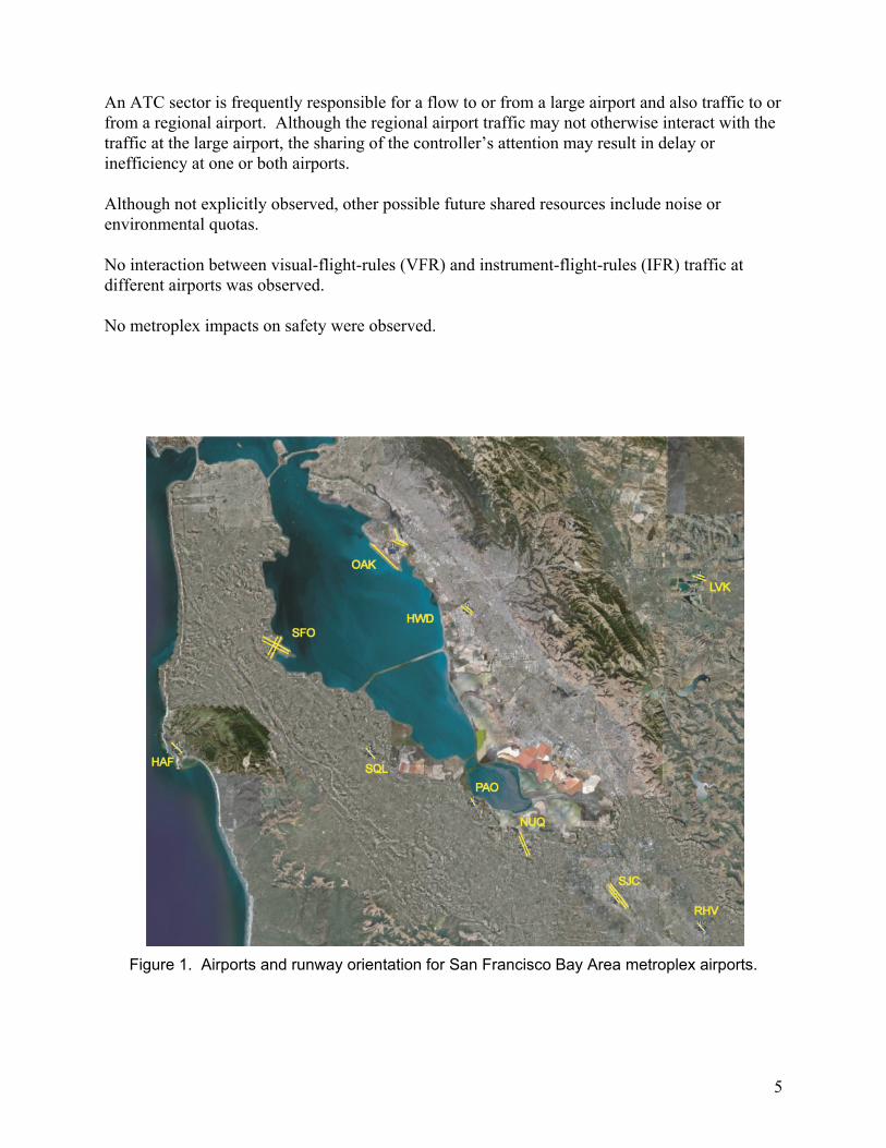
2.3 San Francisco Bay Area Metroplex The project focused on the San Francisco Bay Area metroplex (Figure 1), which contains three large airports—San Francisco International Airport (SFO), Oakland International Airport (OAK), and San Jose International Airport (SJC); four regional airports—Hayward (HWD), San Carlos (SQL), Palo Alto Airport (PAO), Reid-Hillview Airport (RHV); and Moffett Federal Airfield, Moffett Field, California (NUQ). Half Moon Bay Airport (HAF) and Livermore Airport (LVK) do not appear to significantly interact with the other airports, possibly because they are separated from the other airports by terrain (hills). SFO and OAK are separated by 10 miles, while SJC is 30 miles to the south. A conference paper [1] and a NASA Airspace Systems Program Technical Interchange Meeting (TIM) presentation [7] contain considerable detail about the phenomena observed at this metroplex. Figure 2 shows radar track data of arrival and departure flows for the three largest of these airports during a single day, while Figure 3 shows a typical pattern during South-East Plan operations.

2.4 Generalized Metroplex Observations All of the metroplex phenomena observed to date result from a limited resource being shared by operations at different airports. Sharing of several types of resources was observed. Specific points in the local airspace, such as arrival fixes and departure fixes, may be shared. Downstream resources may be shared, resulting in departure operations being subject to combined Traffic Management Initiatives (TMIs) such as miles in trail (MIT). Specific local trajectories may be shared, such as standard terminal arrival routes (STARs) or departure procedures (DPs, also known as SIDs). Airspace where trajectories to or from different airports cross, or would cross if not procedurally separated (e.g., using altitude restrictions), may be shared.

5

An ATC sector is frequently responsible for a flow to or from a large airport and also traffic to or from a regional airport. Although the regional airport traffic may not otherwise interact with the traffic at the large airport, the sharing of the controller’s attention may result in delay or inefficiency at one or both airports. Although not explicitly observed, other possible future shared resources include noise or environmental quotas. No interaction between visual-flight-rules (VFR) and instrument-flight-rules (IFR) traffic at different airports was observed. No metroplex impacts on safety were observed.

Figure 1. Airports and runway orientation for San Francisco Bay Area metroplex airports.

6

Figure 2. Arrival and departure traffic at SFO, OAK, and SJC during West Plan operations

on February 29, 2008.

Figure 3. Typical traffic pattern for SFO, OAK, and SJC during South-East Plan operations.

7

Metroplex phenomena are site-specific and detailed. Since the phenomena depend on the airport configurations and procedures in use—and there are a large number of combinations of these configurations and procedures—there are many metroplex configurations, each with distinct phenomena. Several properties were observed to contribute to the presence of metroplex phenomena:

• The geometry of the airports—the distance between airports and relative runway orientation—can affect metroplex phenomena.

• Terrain and noise restrictions contribute to the presence of metroplex phenomena by reducing the available airspace near the airports.

• Wind direction and speed (and also noise considerations) can affect the runway configurations in use at each airport.

• Visibility (i.e., whether or not visual approaches are allowed) determines procedures in use at each airport. Visibility also affects the volume of IFR traffic. For example, HWD, OAK, and SJC serve numerous flights that typically operate VFR but, when the weather necessitates, operate IFR.

• Time of day can affect the procedures in use, for example if noise restrictions are different between day and night.

• Limited procedures, such as overnight when more strict noise restrictions are in effect, result in metroplex phenomena that do not occur when other procedures are available.

2.5 Generalized Metroplex Management Approaches Metroplex phenomena are visible in current operations, but they result in only small delays (except possibly at New York); in many cases, however, the trajectories are less efficient. Current methods for managing metroplex phenomena can be organized into approaches that 1) spatially decouple the airports, 2) temporally coordinate the use of shared resources, or 3) modify the airspace to minimize the metroplex phenomena. Spatial decoupling uses predefined, conflict-free routes. Because of the limited horizontal extent of the metroplex area, minimum and maximum altitudes are required to allow flows to cross without flight-by-flight coordination. Based on observations to date, spatial separation is the preferred approach to manage interactions where the number of flights that exhibit the interaction is large (i.e., between large airports). This approach makes intuitive sense because spatial decoupling minimizes controller workload. The primary airport generally is given routes that exhibit minimal impact due to the presence of the other airports. Routes to and from the other large airports are then designed around, over, and under the routes of the primary airport, producing decoupled traffic but less-efficient trajectories.

8

The Federal Aviation Administration (FAA) has built large consolidated terminal radar approach control facilities (TRACONs) in several of the regions that currently exhibit metroplex issues, including New York, Los Angeles basin, and the San Francisco Bay Area, suggesting that the FAA has already reacted to the need to manage metroplex phenomena. The creation of these large TRACONs facilitates airspace design that decouples the major airports in the region. Temporal deconfliction (i.e., coordinating the times at which individual flights may use a shared resource) appears to be the preferred approach when the number of flights that exhibit the interaction is small. This may be the preferred approach due to not wanting to over-constrain the predefined routes used for the large airports; spatially separating the routes to and from large airports and small airports with little daily traffic may require too many routes, forcing each to be contained to a smaller area. Without automation, temporal deconfliction requires significant workload to select when each flight may use the shared resource and then control each flight to comply. However, temporal deconfliction provides a solution in situations where the proximity and geometry of the airports preclude the use of static, spatial deconfliction. Temporal deconfliction also is (currently) inefficient because of the uncertainty in when each flight will actually use the shared resource, requiring some slack between operations. NextGen technologies could make temporal deconfliction much more efficient. Both spatial and temporal approaches are predefined through published procedures. These procedures are typically described in STARs, DPs (or SIDS), local standard operating procedures (SOPs), and letters of agreement (LOAs). Airport runway configurations are varied because of weather and other factors, such as balancing noise exposure. Separate procedures are defined for each combination of airport configuration, and some combinations are more efficient than others. Therefore, the coordination of runway configurations used at each airport to create the most efficient, feasible metroplex configuration adds a time-varying element to metroplex management and is the third class of current techniques used to manage metroplex phenomena. New York’s use of this class of approach includes reallocating a piece of airspace between LaGuardia International Airport (LGA) and John F. Kennedy International Airport (JFK). Access to the airspace enables either airport to use an additional procedure that increases the capacity of that airport. Note that significant overlap exists between traffic management at a metroplex and at a busy single airport. The types of dependencies between two closely spaced airports, each with one runway, are very similar to those observed between runways at a single airport with multiple runways. Moreover, the approaches used to manage metroplex phenomena and busy single airports are similar. For example, managing release times to coordinate departures from metroplex airports on common or crossing trajectories is similar to using release times to achieve MIT spacing for consecutive departures to a common departure fix at a busy single airport. Metroplex management also exhibits the common phenomena that local procedures have evolved to meet specific local needs, and have been created by local individuals using their experience and preference, but have not been optimized.

9

In summary, spatial deconfliction decouples airports, results in little or no capacity loss due to the metroplex phenomena, requires some less-efficient trajectories, and gives preference to the larger airports. Temporal coordination is currently inefficient because the point at which aircraft are controlled is often separate from the shared resource, and uncertainties (both in compliance with the controlled time and between the control point and the shared resource) require significant safety buffers. Temporal coordination permits efficient trajectories but creates a direct capacity trade-off between airports, as well as higher controller workload currently. Dynamic airspace and temporal coordination are currently underutilized. Dynamic airspace has the potential to match resource allocation to demand, where the demand characteristics vary in time.

3 METROPLEX DEFINITION

The Joint Planning and Development Office (JPDO) Concept of Operations for the Next-Generation Air Transportation System (NGATS) [8] has defined a metroplex as “a group of two or more adjacent airports whose arrival and departure operations are highly interdependent”. Although easy to understand, this definition does little to describe metroplex characteristics or suggest methods for managing a metroplex. Precisely drawing a line around a metroplex is not likely to be a tremendously useful way to define the metroplex. For example, operations at one airport within the physical boundary of a metroplex might be decoupled, for some reason, from operations at the other airports. Two metroplexes might overlap, sharing some airports but not others. A good definition must address the need to which it is applied. In this project, the definition should help guide further research and coordination with other NGATS research. Consequently, we focused on definitions that captured the type and extent of the interdependencies rather than the metroplex geometry. A metroplex definition should provide a common foundation for discussing metroplexes. Furthermore, the definition should be useful to locate, quantify, and compare metroplexes by measuring their type and magnitude. Lastly, the definition should provide insight into methods for managing metroplex traffic.

3.1 Qualitative Metroplex Definition To facilitate modeling the effect of metroplexes in Next-Generation Air Transportation System (NextGen) and studying concepts for managing metroplex phenomena, a metroplex definition was sought that captures the type, magnitude, and impact of interdependencies rather than a geographic boundary. A qualitative metroplex definition was offered first [9]. A metroplex is a set of airports that exhibit metroplex phenomena. Metroplex phenomena, we defined, as interdependencies between operations at two or more closely spaced airports that cause a reduction in capacity, efficiency, or safety (or an increase in environmental impact) at one or more of the airports, relative to what the operations at those airports would be if each airport were the only airport. The interdependencies are considered to be fundamental to the

10

metroplex; they result from the geometry, aircraft separation standards, aircraft performance characteristics, and the aircraft types that use the airports. The types of impacts that result from metroplex interdependencies depend on the coordination used to manage the interdependencies. For example, spatial deconfliction may result in no capacity trade-off between the airports but less-efficient trajectories for one or both airports, while temporal deconfliction may result in optimal trajectories for each airport but a capacity trade-off between the airports. Fundamentally, metroplex management includes an element of balancing competing objectives—efficiency and capacity. The magnitude of the impacts further depends on the amount of traffic, and requires a baseline to measure, chosen to be a hypothetical situation in which the other nearby airports do not exist. Therefore, a set of airports may have the potential to be a metroplex because of interdependencies but may not exhibit metroplex phenomena because either traffic volume is too low or coordination methods in use mitigate the impact of the interdependencies. Note that temporal deconfliction would produce no delays when there is insufficient traffic at both airports, while spatial deconfliction may still result in measurable increase in distance flown. Some metroplex impacts are difficult to measure in current operations because of the management approaches already being applied. For example, measuring the impact of metroplex phenomena that are managed through procedures that spatially decouple operations to and from different airports is challenging since the baseline—what the trajectories would be in the absence of other airports—requires judgment. Other factors, such as terrain and noise restrictions, can also influence trajectories close to the airport.

3.2 Types of Quantitative Definitions Our original goal was to introduce a unified metroplex definition as well as a set of dimensions along which metroplexes may be measured. However, as we studied a variety of methods for measuring metroplex phenomena, we demonstrated that different analytic definitions are useful for describing different aspects of metroplex phenomena, but no one definition provides a complete picture. We classified definitions into three types [10]—observation-based or “black box,” model-based or microscopic, and simulation-based. Observation-based definitions treat the metroplex as a black box. These definitions attempt to quantify metroplex characteristics from the relationship between observable input and output data. Therefore, these definitions attempt to avoid the need for detailed knowledge of local procedures. As a result, this approach can readily be applied to a large number of potential metroplexes. However, separating metroplex interactions from other effects such as noise restrictions can be infeasible without applying local knowledge. This type of definition may be applied to real-world data or simulation outputs. However, the baseline against which to measure the impact of the metroplex phenomena is not well defined, often requiring comparisons against other airports rather than on an absolute basis. In fact, the metroplex phenomena and result of current management approaches are combined in the result. Lastly, this type of definition does not directly support identifying viable metroplex management approaches.

11

We studied a variety of observation-based metrics [10] such as excess distance flown and several airspace complexity metrics. Husni Idris studied the New York metroplex using a queuing model that is an example of observation-based metrics [3], [4], and [11]. Model-based (or microscopic) definitions require detailed knowledge of local procedures, making them harder to apply to future environments. However, definitions in this class excel at visualizing metroplex phenomena and identifying effective traffic management approaches. Our approach to this type of definition was to extend the classic arrival-departure capacity curve by adding additional constraints (in various dimensions) to model the metroplex phenomena, such as shared use of a departure fix or piece of airspace [9]. The approach, like many of the potential definitions, was useful for some reasons but awkward for describing some impacts of interdependencies such as less-efficient trajectories or capturing restrictions on timing of events, which can result in delays without affecting capacity. Simulation-based definitions are ideal for comparing alternative management concepts and studying future environments or traffic levels. We employed a simulation-based definition throughout our study of metroplex management concepts.

4 METROPLEX MODELING

Metroplex modeling activities during the project may be grouped into three areas: assessing the current cost of metroplex phenomena, developing part-metroplex models of specific types of metroplex phenomena, and developing a simulation environment for studying metroplex management concepts.

4.1 Modeling Current Metroplex Costs The purpose of modeling current metroplex operations was to better understand the existing magnitude of the lost capacity or inefficiencies due to metroplex phenomena. We focused on two interactions in the San Francisco Bay Area: coordination of San Francisco (SFO) and Oakland (OAK) departures during quiet and silent operations and Hayward (HWD) instrument-flight-rules (IFR) departures blocking Oakland (OAK) arrivals. Using actual traffic data from a single day in West Plan (runway use plan), we modeled the operations independently for each airport and compared those results to a model of both airports operating with the metroplex interaction. Table 1 shows the results for the SFO-OAK interaction. Overnight, to reduce the residential noise impact, both SFO and OAK departures stay over the center of the bay, requiring departures from the two airports to be merged into a common stream immediately upon takeoff. SFO and OAK share the capacity of this one stream, and departures must be coordinated in time to enable the merge.

12

TABLE 1. MODELED SFO-OAK SILENT/QUIET DELAYS

SFO OAK Total

Departures (number of flights) 83 42 125

Without metroplex dependency (min:sec delay)

2:35 0:23 2:58

With metroplex dependency (min:sec delay)

19:58 15:54 35:52

Similarly, the metroplex interaction added approximately 2 minutes of delay per HWD departure, and 19 HWD departures caused 93 minutes of arrival delay at OAK. Additional information about our modeling of current metroplex operations appears in reference [12].

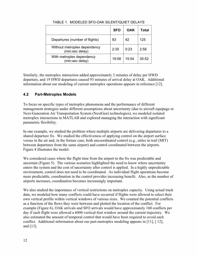
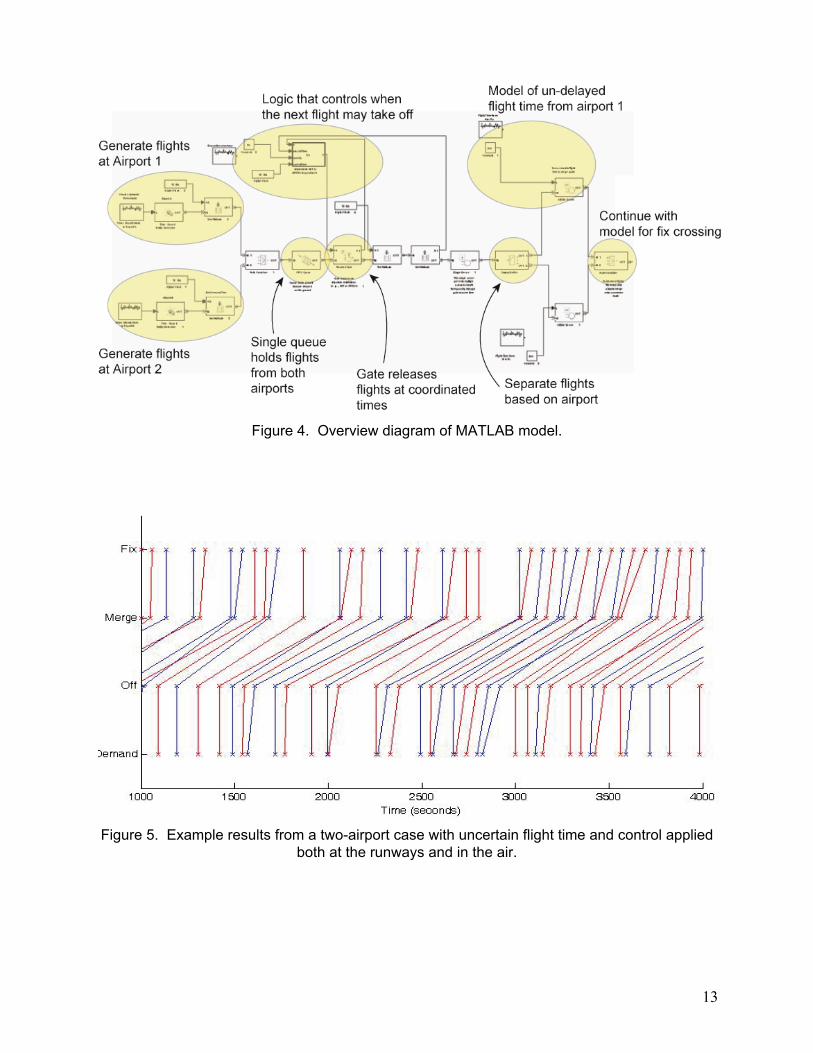
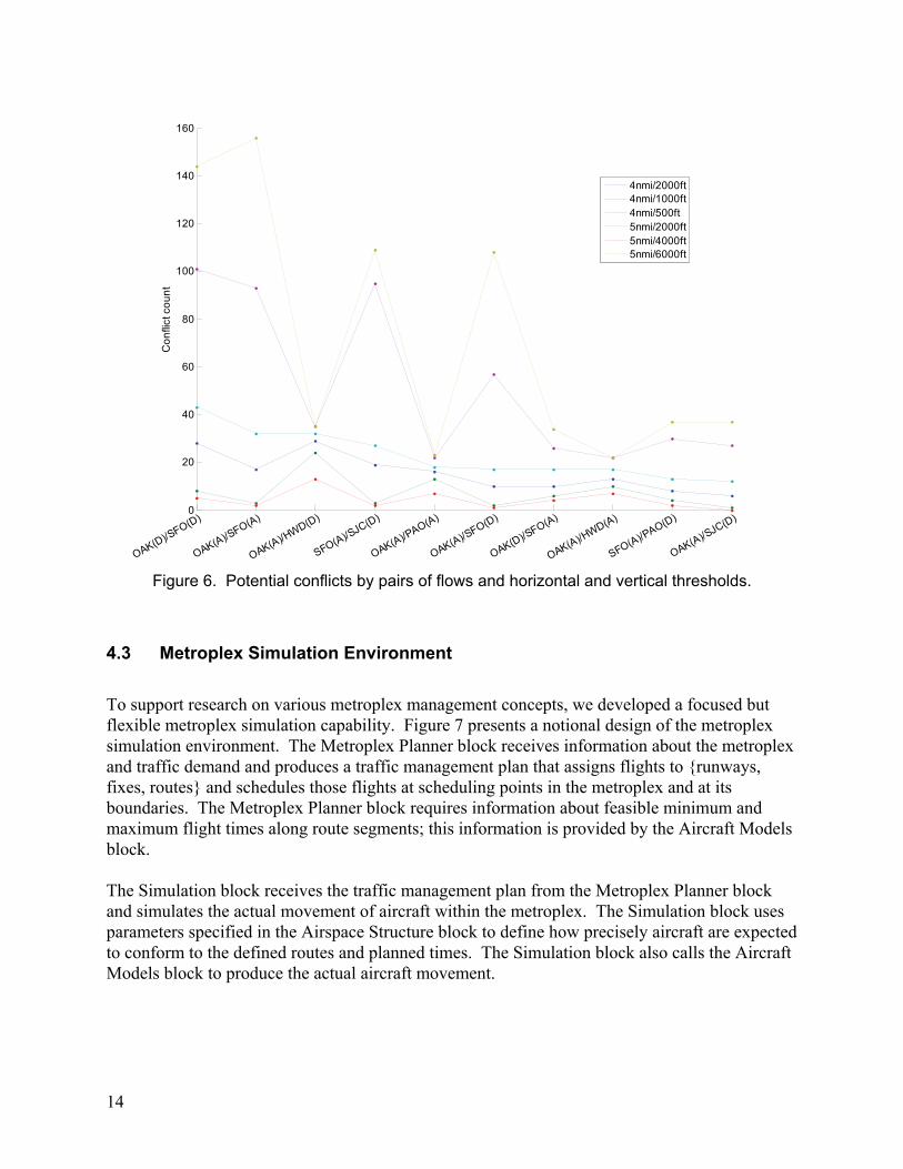
4.2 Part-Metroplex Models To focus on specific types of metroplex phenomena and the performance of different management strategies under different assumptions about uncertainty (due to aircraft equipage or Next-Generation Air Transportation System (NextGen) technologies), we modeled isolated metroplex interactions in MATLAB and explored managing the interaction with significant parametric flexibility. In one example, we studied the problem where multiple airports are delivering departures to a shared departure fix. We studied the effectiveness of applying control on the airport surface versus in the air and, in the former case, both uncoordinated control (e.g., miles in trail (MIT) between departures from the same airport) and control coordinated between the airports. Figure 4 illustrates the model. We considered cases where the flight time from the airport to the fix was predictable and uncertain (Figure 5). The various scenarios highlighted the need to know where uncertainty enters the system and the cost of uncertainty after control is applied. In a highly unpredictable environment, control does not need to be coordinated. As individual flight operations become more predictable, coordination in the control provides increasing benefit. Also, as the number of airports increases, coordination becomes increasingly important. We also studied the importance of vertical restrictions on metroplex capacity. Using actual track data, we modeled how many conflicts could have occurred if flights were allowed to select their own vertical profile within vertical windows of various sizes. We counted the potential conflicts as a function of the flows they were between and plotted the location of the conflict. For example (Figure 6), OAK arrivals and SFO arrivals would have approximately 160 conflicts per day if each flight were allowed a 6000-vertical-foot window around the current trajectory. We also estimated the amount of temporal control that would have been required to avoid each conflict. Additional information about our part-metroplex modeling appears in [11], [ 12], and [13].

13

Figure 4. Overview diagram of MATLAB model.

Figure 5. Example results from a two-airport case with uncertain flight time and control applied both at the runways and in the air.

14

Figure 6. Potential conflicts by pairs of flows and horizontal and vertical thresholds.

4.3 Metroplex Simulation Environment

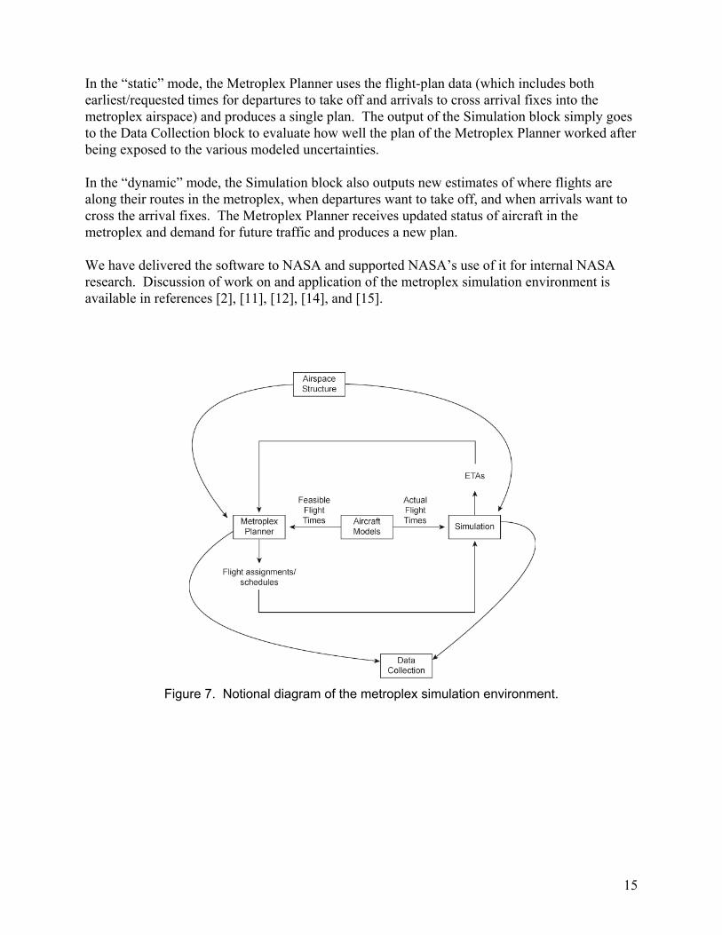
To support research on various metroplex management concepts, we developed a focused but flexible metroplex simulation capability. Figure 7 presents a notional design of the metroplex simulation environment. The Metroplex Planner block receives information about the metroplex and traffic demand and produces a traffic management plan that assigns flights to {runways, fixes, routes} and schedules those flights at scheduling points in the metroplex and at its boundaries. The Metroplex Planner block requires information about feasible minimum and maximum flight times along route segments; this information is provided by the Aircraft Models block. The Simulation block receives the traffic management plan from the Metroplex Planner block and simulates the actual movement of aircraft within the metroplex. The Simulation block uses parameters specified in the Airspace Structure block to define how precisely aircraft are expected to conform to the defined routes and planned times. The Simulation block also calls the Aircraft Models block to produce the actual aircraft movement.

0

20

40

60

80

100

120

140

160

Co

nfli

ct c

ou

nt

OAK(D)/SFO(D)

OAK(A)/SFO(A)

OAK(A)/HWD(D)

SFO(A)/SJC(D)

OAK(A)/PAO(A)

OAK(A)/SFO(D)

OAK(D)/SFO(A)

OAK(A)/HWD(A)

SFO(A)/PAO(D)

OAK(A)/SJC(D)

4nmi/2000ft4nmi/1000ft4nmi/500ft5nmi/2000ft5nmi/4000ft5nmi/6000ft

15

In the “static” mode, the Metroplex Planner uses the flight-plan data (which includes both earliest/requested times for departures to take off and arrivals to cross arrival fixes into the metroplex airspace) and produces a single plan. The output of the Simulation block simply goes to the Data Collection block to evaluate how well the plan of the Metroplex Planner worked after being exposed to the various modeled uncertainties. In the “dynamic” mode, the Simulation block also outputs new estimates of where flights are along their routes in the metroplex, when departures want to take off, and when arrivals want to cross the arrival fixes. The Metroplex Planner receives updated status of aircraft in the metroplex and demand for future traffic and produces a new plan. We have delivered the software to NASA and supported NASA’s use of it for internal NASA research. Discussion of work on and application of the metroplex simulation environment is available in references [2], [11], [12], [14], and [15].

Figure 7. Notional diagram of the metroplex simulation environment.

16

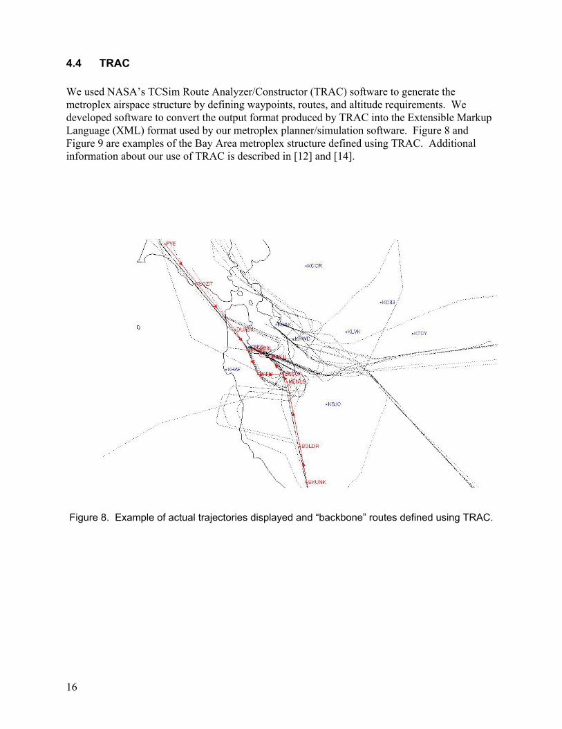
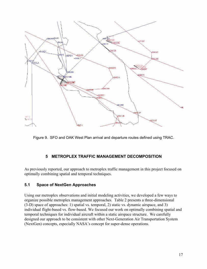
4.4 TRAC We used NASA’s TCSim Route Analyzer/Constructor (TRAC) software to generate the metroplex airspace structure by defining waypoints, routes, and altitude requirements. We developed software to convert the output format produced by TRAC into the Extensible Markup Language (XML) format used by our metroplex planner/simulation software. Figure 8 and Figure 9 are examples of the Bay Area metroplex structure defined using TRAC. Additional information about our use of TRAC is described in [12] and [14].

Figure 8. Example of actual trajectories displayed and “backbone” routes defined using TRAC.

17

Figure 9. SFO and OAK West Plan arrival and departure routes defined using TRAC.

5 METROPLEX TRAFFIC MANAGEMENT DECOMPOSITION

As previously reported, our approach to metroplex traffic management in this project focused on optimally combining spatial and temporal techniques.

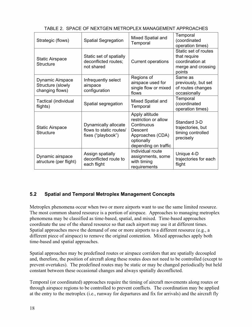
5.1 Space of NextGen Approaches Using our metroplex observations and initial modeling activities, we developed a few ways to organize possible metroplex management approaches. Table 2 presents a three-dimensional (3-D) space of approaches: 1) spatial vs. temporal, 2) static vs. dynamic airspace, and 3) individual flight-based vs. flow-based. We focused our work on optimally combining spatial and temporal techniques for individual aircraft within a static airspace structure. We carefully designed our approach to be consistent with other Next-Generation Air Transportation System (NextGen) concepts, especially NASA’s concept for super-dense operations.

18

TABLE 2. SPACE OF NEXTGEN METROPLEX MANAGEMENT APPROACHES

Strategic (flows) Spatial Segregation Mixed Spatial and Temporal

Temporal (coordinated operation times)

Static Airspace Structure

Static set of spatially deconflicted routes; not shared

Current operations

Static set of routes that require coordination at merge and crossing points

Dynamic Airspace Structure (slowly changing flows)

Infrequently select airspace configuration

Regions of airspace used for single flow or mixed flows

Same as previously, but set of routes changes occasionally

Tactical (individual flights)

Spatial segregation Mixed Spatial and Temporal

Temporal (coordinated operation times)

Static Airspace Structure

Dynamically allocate flows to static routes/ fixes (“playbook”)

Apply altitude restriction or allow Continuous Descent Approaches (CDA) optionally depending on traffic

Standard 3-D trajectories, but timing controlled precisely

Dynamic airspace atructure (per flight)

Assign spatially deconflicted route to each flight

Individual route assignments, some with timing requirements

Unique 4-D trajectories for each flight

5.2 Spatial and Temporal Metroplex Management Concepts Metroplex phenomena occur when two or more airports want to use the same limited resource. The most common shared resource is a portion of airspace. Approaches to managing metroplex phenomena may be classified as time-based, spatial, and mixed. Time-based approaches coordinate the use of the shared resource so that each airport may use it at different times. Spatial approaches move the demand of one or more airports to a different resource (e.g., a different piece of airspace) to remove the original contention. Mixed approaches apply both time-based and spatial approaches. Spatial approaches may be predefined routes or airspace corridors that are spatially decoupled and, therefore, the position of aircraft along these routes does not need to be controlled (except to prevent overtakes). The predefined routes may be static or may be changed periodically but held constant between these occasional changes and always spatially deconflicted. Temporal (or coordinated) approaches require the timing of aircraft movements along routes or through airspace regions to be controlled to prevent conflicts. The coordination may be applied at the entry to the metroplex (i.e., runway for departures and fix for arrivals) and the aircraft fly

19

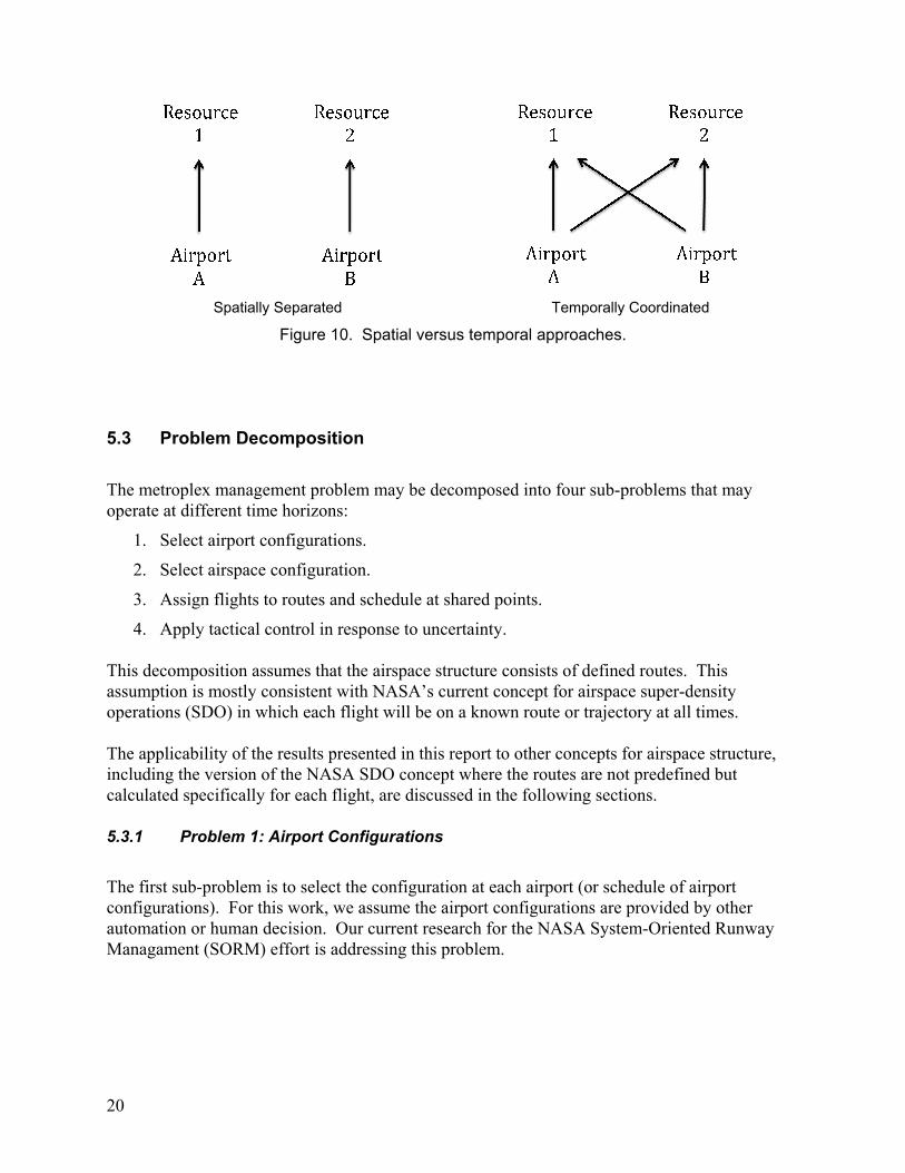
open-loop through the metroplex, or applied at various points or continuously through the metroplex airspace. Four-dimensional trajectories—defining unique trajectories for each flight that are decoupled where a piece of airspace may be used by different airports at different times—is an approach that combines spatial and time-based approaches. Examples of other shared resources are controller attention and environmental quotas. Temporal approaches applied to contention for these resources similarly deconflict the use of the resource in time. Spatial approaches involve modifying the demand to use a different resource; this approach may not be available without changing the resources, such as what controllers work what airspace. In this report, we primarily consider contention for airspace resources between metroplex airports. There is a trade-off between capacity and efficiency. The San Jose (SJC) loop departure procedures are a good example. The SJC departures and San Francisco (SFO) arrivals could be coordinated in time to avoid the need for the longer path length flown by the SJC departures. However, during periods of simultaneous demand, some flights would be delayed by this coordination, reducing the total number of operations in the metroplex during those periods of time. Historically, maximizing capacity has been the principal objective in air traffic management research. Recently, fuel-efficiency considerations have moved to the forefront as traffic has decreased, fuel costs have increased, and environmental considerations have become more important. We can expect over the lifetime of any metroplex management concept that the relative importance of different objectives will vary. In fact, the blending of objectives may vary as a function of time of day in some situations. Therefore, we strive to propose approaches that are flexible to relatively weighting different objectives. The optimal trade-off between spatial and temporal approaches to managing metroplex operations depends on the technologies available for time-based coordination. Historically, spatial approaches have been applied when possible to decouple operations at metroplex airports. Spatial approaches have been more efficient than temporal approaches because a lack of good coordination automation has made temporal coordination require higher workload, and large uncertainty requires large safety buffers between consecutive operations. However, one result of dedicating different corridors of airspace to each airport is that each airport has fewer departure corridors. As a result, additional spacing is often required between consecutive departures from the airport, since diverging headings are not available. Moreover, during periods of high demand at one airport but low demand at other metroplex airports, the static airspace structure does not allow the busy airport to take advantage of underutilized airspace allocated to the other airports. Figure 10 illustrates the difference between static allocation of spatially separated routes and shared routes on which operations must be coordinated in time, using an example in which there are two airports and two resources (e.g., routes or departure fixes). In a NextGen environment, precise temporal coordination and precise compliance with planned resource usage times could allow temporal coordination to be much more efficient than in current operations and provide more different departure corridors to each airport. An interim approach may be to dynamically reallocate resources to each airport, where at any point in time the allocations are spatially decoupled.

20

Spatially Separated Temporally Coordinated

Figure 10. Spatial versus temporal approaches.

5.3 Problem Decomposition

The metroplex management problem may be decomposed into four sub-problems that may operate at different time horizons:

1. Select airport configurations.

2. Select airspace configuration.

3. Assign flights to routes and schedule at shared points.

4. Apply tactical control in response to uncertainty. This decomposition assumes that the airspace structure consists of defined routes. This assumption is mostly consistent with NASA’s current concept for airspace super-density operations (SDO) in which each flight will be on a known route or trajectory at all times. The applicability of the results presented in this report to other concepts for airspace structure, including the version of the NASA SDO concept where the routes are not predefined but calculated specifically for each flight, are discussed in the following sections. 5.3.1 Problem 1: Airport Configurations

The first sub-problem is to select the configuration at each airport (or schedule of airport configurations). For this work, we assume the airport configurations are provided by other automation or human decision. Our current research for the NASA System-Oriented Runway Managament (SORM) effort is addressing this problem.

21

5.3.2 Problem 2: Airspace Configuration

For the given set of airport configurations (or schedule of configurations), we must create the route structure. If a unique 4-D trajectory will be defined for each flight, this step may still define some airspace allocation, such as what fixes are being used or what regions of airspace will be used for only specific traffic flows. If a playbook of predefined sets of routes is used, then this step selects the set of routes (or schedule of sets). The simplest case is that a single “play” exists for each set of airport configurations. Between these extremes, routes are defined (as opposed to unique 4-D trajectories) but are not predefined; a set of routes is defined to be optimal for current conditions. This option likely does not offer significant advantage over the “playbook” approach. 5.3.3 Problem 3: Flight Planning

If the airspace configuration uses defined, known routes, then the metroplex flight planning problem, which was the focus of our work, is to assign each flight to a route through the metroplex (which may include assigning the transition fix and runway) and scheduling the flight at certain points along that route to avoid conflicts at intersections (which include runways and transition fixes). Vertical restrictions could be applied as an additional dimension of control or could be applied by predefining multiple routes with different vertical constraints (e.g., a route with vertical flexibility and a separate route with vertical restrictions to spatially eliminate crossing points). If the airspace configuration concept defines only regions of airspace available for each flow and allows flight-unique trajectories, then the flight planning problem takes a different form, which we did not study in this project. 5.3.4 Problem 4: Tactical Corrections

Once the aircraft is flying along the route, airborne control may be required to react to compliance errors or other uncertainties. One modeling option is to set the uncertainties (e.g., compliance with a route and error in the predicted speed) to equal values that represent the motion of the aircraft after airborne control is applied. Another research option is to study the prior steps in an environment where airborne control is not available. 5.3.5 Relevance to Research

This decomposition of the metroplex management problem, we believe, handles most concepts for airspace structure within which the metroplex management problem must operate. The concept in which each flight receives unique 4-D trajectories is distinct. Such a concept requires a slightly different decomposition—effectively dividing the airspace configuration problem (problem 2 described previously) into two parts. The first part defines the regions of airspace available for the 4-D trajectories. The remainder of the airspace configuration problem—defining the “routes”—is combined with the flight planning problem (problem 3 described

22

previously) since defining the “routes” and assigning flights to routes (and scheduling them along the routes) are actually the same problem when each flight is assigned a unique trajectory. Problems 1 and 2 could likely be combined. However, problem 1, the airport configuration selection, is the focus of other work and is not studied here, motivating the separation. Problem 2 was studied briefly by solving problem 3 for different airspace structures and comparing, rather than building an optimization algorithm to solve problem 2 in a real-time automation system. The latter is proposed for future work. Problem 4, which is not unique to metroplexes, could be studied by considering whether or not speed control is sufficient to maintain separation at intersection points, given an assumption about aircraft equipage/technology and the resulting compliance errors and prediction uncertainty. Problem 3 was our focus. We developed a “static” metroplex planner that produces a set of assignments and scheduled times on a single set of input data. We further applied this static planner within a dynamic planner—one that uses time windows and freeze horizons to incrementally advance the solved time window while using new information about flights further away in time. That work is described at the beginning of this report as well as in references [2], [11], [12], [14], and [15].

6 METROPLEX PLANNER INTRODUCTION

This section describes the evolution of our thinking and approach to solving the problem of managing metroplex operations. Atkins [1] summarized numerous metroplex phenomena, particularly in the San Francisco Bay Area, illustrating the current use of both spatial deconfliction (i.e., use alternate routes or resources) and temporal coordination (i.e., interleave utilization of shared resources) to manage different metroplex interactions. Enabling Nest-Generation Air Transportation System (NextGen) technologies will allow more dynamic selection of a spatial or temporal solution to a metroplex interaction, either on a flight-by-flight basis or for flows during a period of time. Our goal, therefore, became to develop an algorithm to optimally choose between spatial and temporal approaches to manage metroplex interactions. The point of departure for this research was the realization that a predominant factor contributing to metroplex operations is the need for sharing of critical resources across multiple airports within the metroplex—whether those resources be airspace, information, or controller attention. If we consider existing techniques that have been put in place to manage metroplex interactions at various locales throughout the National Airspace System (NAS), we can broadly place these approaches into two major categories: spatial strategies and temporal strategies. Spatial strategies handle potential conflicts by defining completely separate physical “corridors” for aircraft to travel within, where the corridors themselves have been procedurally deconflicted. An example is the use of altitude restrictions on departures climbing out of a given airport such that

23

the departures will stay below the arrival streams of another airport. Temporal strategies, on the other hand, use explicit timing of individual flight operations to interleave aircraft through the shared resource. As it turns out, however, the “best” strategy to apply in a given situation depends on many factors, and it generally can change over time. Given this classification, our approach was to pose the metroplex traffic management problem in the context of an optimization problem. Rather than solve the route assignment, sequencing, and scheduling problems as a series of sub-problems, we instead attempted to solve these problems simultaneously. We desired to see whether the appropriate management strategy (spatial vs. temporal) in a given situation could fall out “naturally” from the optimization—as opposed to having to be defined a priori as in current-day operations. In this sense, the approach applied could change minute-by-minute or flight-by-flight. We thus set out to formulate the metroplex problem in an optimization context. Inspirations came from previous work on surface routing and scheduling—where considerable research has been conducted on optimization algorithms related to conflict-free scheduling of surface movements. Table 3 summarizes the key references that influenced our thinking and highlights how each reference modeled the various functions: route assignment, sequencing, and scheduling. In particular, we began by studying the taxi scheduling work of Rathinam, Montoya, and Jung [13], which, although not handling the route assignment problem (taxi routes were assumed to be defined a priori), developed a mixed integer sequencing and scheduling problem similar to that which we were seeking. It should be noted, however, that the results reported in their paper correspond to a pure linear program; the binary sequencing variable values were set through a preprocessing step based on “first come, first-served” (FCFS) ordering. Nonetheless, the ideas expressed in the paper significantly influenced our thinking. We studied other surface optimization formulations that included both routing and scheduling aspects—but modeling time as discrete with discrete routing decisions at each node (Marin [16]; Roling and Visser [17]; and Smeltink, Soomer, DeWaal, and Van Der Mei [18]). We developed initial prototype implementations of several of these formulations to assess their numerical performance. At least given the solvers we had readily available, however, the realistic size of the problems that could be solved in any sort of reasonable time was limited. The formulation presented in Keith, Richards, and Sharma [19] was the closest to what we were looking for, namely modeling discrete routing and sequencing decisions and continuous time scheduling. However, their approach treated each node within the network as a discrete decision point, resulting in a discrete decision variable space significantly larger than what we thought was necessary. The formulation presented in the following sections represents our fusion of the inspiration provided by these previous efforts. The basic formulation, presented in Capozzi, Atkins, and Choi [2], is similar to that of Keith, Richards, and Sharma [19], but rather than treating each turn as a discrete decision, treats routing options in the form of complete routes. For our purposes, rather than scheduling, sequencing, and deconflicting at every point along a route, it is only strictly necessary to make decisions at key points that “matter”—particularly where flights can potentially conflict given underlying route geometry. As described in the following sections, however, the dynamic form of the problem (e.g., planning “in front of the aircraft” as it moves along its most current plan) begins to resemble that of Keith, et. al.

24

In the dynamic planning application, we solve a sequence of deterministic problems. Each problem comprises a “demand snapshot”, a “route network”, and a function that maps route options onto each flight in the demand set. The general concept is to over-specify the route option set to include options representative of both spatial and temporal strategies. In this fashion, the metroplex management strategy to use can naturally fall out of the optimization process. As stated previously, our objective in this facet of the research conducted under this NASA research announcement (NRA) effort was to develop an approach to simultaneously and optimally solve the route assignment, sequencing, and scheduling problems in the context of metroplex operations. From an algorithm perspective, this work extends NASA’s prior scheduling-only work to include route assignment and could be applied to ongoing Safe and Efficient Surface Operations (SESO) research. This problem is a challenging one—primarily because of the dimensionality of the underlying discrete state space. However, it should be noted that it was not our intention to leverage expensive, state-of-the-art solvers and to be content in solving the problem at all, regardless of how long it took. Rather, we focused on the development of an optimization-based formulation that could be solved with open-source solvers in the context of a real-time automation system—practical optimization.

TABLE 3. SUMMARY OF KEY REFERENCES THAT SHAPED THE MILP FORMULATION DEVELOPED IN THIS RESEARCH

Reference Routing Sequencing Scheduling

Smeltink et al., 2005 N/A Binary Continuous

Rathinam et al., 2008 N/A Binary3 Continuous

Roling and Visser, 2008 Discrete at each node Binary Discrete

Marin, 2006 Discrete at each node Binary Discrete

Keith et al., 2008 Discrete at each node Binary Continuous

Capozzi et al., 2009 Discrete at route level Binary Continuous

3Although the formulation described in this paper included binary sequencing variables, the results presented were

obtained by first setting the values of the binary variables based on first-come, first-served (FCFS) scheduling. The remaining problem was a pure linear program with only continuous variables remaining.

25

7 FORMULATION AS A MIXED INTEGER LINEAR PROGRAM

This section describes the approach taken to achieve the capability of simultaneously and optimally solving the route assignment, sequencing, and scheduling problem—namely, casting the problem in the form of a mixed integer linear program (MILP). This choice was a natural one given the discrete nature of the routing and sequencing decisions and the continuous nature of the scheduling aspects of the problem. This section describes the MILP “kernel” that is used to solve a given deterministic problem instance within the overall dynamic planning framework.

7.1 Preliminaries and Notation The geographical scope of the problem to be solved is taken to be the combined terminal maneuvering area for the set of airports included in a given metroplex. From a modeling perspective, we define a point at a virtual metroplex “center” and draw an arc at a distance of approximately 200 nautical miles (nmi) from this center point. This arc defines the boundary at which arriving flights are assumed to “enter” the metroplex and the point at which departures are assumed to “exit” the metroplex. The demand set to be modeled includes arrivals and departures into and/or out of any or all of the metroplex airports (see Figure 11), in one of various operational “phases”:

• Arrival flights outside the metering fixes, en route to one of the metroplex airports

• Arrival flights inside the metering fixes, en route to one of the metroplex airports

• Departing flights waiting to push from the gate

• Departing flights taxiing to the runways

• Airborne departures en route, exiting the metroplex The following assumptions are utilized in establishing a given problem instance:

• The set of flights to be scheduled is . An individual flight is denoted by .

• We assume the existence of a globally defined set of complete routes, . Each route uniquely connects a metroplex “entry” point to a metroplex “exit” point.

• Each flight can be feasibly assigned to one or more routes, . We assume the existence of some function that prunes the set of available routes and identifies and populates the subset of route options to be considered for each flight in the demand set.

• Each route contains an ordered set of scheduling points, .

• The initial scheduling point on any given route is denoted by .

• The The final scheduling point4 on any given route is denoted by .

4 In the limit where a “route” consists of only a single scheduling point, we use the “initial” point notation, , to

denote this point. Thus, no “final” point is defined in such cases.

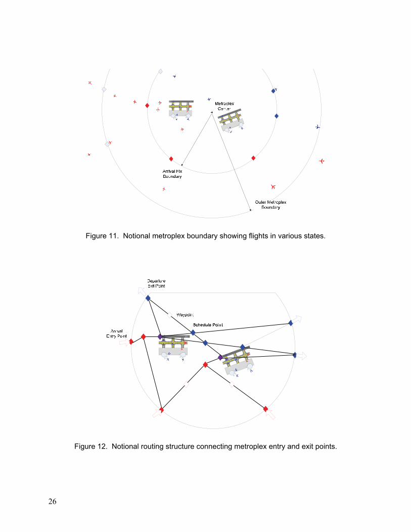
26

Figure 11. Notional metroplex boundary showing flights in various states.

Figure 12. Notional routing structure connecting metroplex entry and exit points.

27

Note that no a priori assumptions are made regarding the routing structure that is defined for a given planning cycle; the route structure is a function solely of the airspace design concept being evaluated. As such, the routing structure may include only a single route from a given arrival fix to a particular arrival runway (thus implicitly defining the airspace and runway configurations). Or, at the other extreme, there may be a route from every arrival fix to every runway in both directions—thus allowing the runway usage to be determined as part of the overall optimization process. Figure 12 shows an example routing structure and highlights several aspects of the associated data, including several “entry” and “exit” points. Note that a formal distinction is made between schedule points—where separation is actively controlled—and waypoints, at which separation is not controlled. The specification of which points in the routing structure “matter” and should be defined as schedule points is left to the user. Similarly, the formulation makes no assumptions regarding the definition of feasible route options for each flight. Rather, the user is provided the flexibility to define the mapping function of choice. Typical mapping functions that might be considered include the following (generally ordered from more to less restrictive):

• Assign a single-route option a priori to each flight, eliminating the route assignment sub-problem and leaving only sequencing and scheduling as free variables.

• Include routes that connect from a given “fix” to a given “runway”. Such a mapping implicitly defines the runway usage/configuration.

• Include routes that connect from a given “fix” to all usable runways at a given “airport”, allowing investigation of the value of relaxing the notion of runway configuration to allow flights to be routed to any usable runway.

• Include routes that connect from a given “entry direction” (e.g., the northeast) to a given airport runway. Such a mapping could be used to explore the value of sharing multiple airspace fixes across several metroplex airports.

• Include routes that connect from a given “entry direction” (e.g., the northeast) to all usable runways at a given airport. Such a mapping could be used to explore the value of sharing multiple airspace fixes across several metroplex airports.

• Include routes that connect from a given “entry direction” to all runways at all airports. Such a mapping could be used to explore the value of distributing traffic across multiple metroplex airports within a geographic region.

As should be clear from these examples, almost any mapping function could be implemented. It should also be noted that the effective routing structure—particularly in the dynamic planning context—changes as flights move through the metroplex (see Figure 13) to include only those portions of route options “in front” of each aircraft.

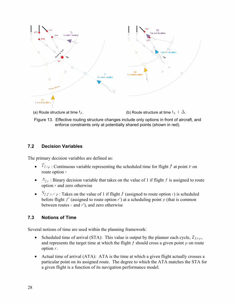
28

(a) Route structure at time . (b) Route structure at time .

Figure 13. Effective routing structure changes include only options in front of aircraft, and enforce constraints only at potentially shared points (shown in red).

7.2 Decision Variables The primary decision variables are defined as:

• : Continuous variable representing the scheduled time for flight at point on route option

• : Binary decision variable that takes on the value of 1 if flight is assigned to route option and zero otherwise

• : Takes on the value of 1 if flight (assigned to route option ) is scheduled before flight (assigned to route option ) at a scheduling point (that is common between routes and ), and zero otherwise

7.3 Notions of Time Several notions of time are used within the planning framework:

• Scheduled time of arrival (STA): This value is output by the planner each cycle, , and represents the target time at which the flight should cross a given point on route option .

• Actual time of arrival (ATA): ATA is the time at which a given flight actually crosses a particular point on its assigned route. The degree to which the ATA matches the STA for a given flight is a function of its navigation performance model.

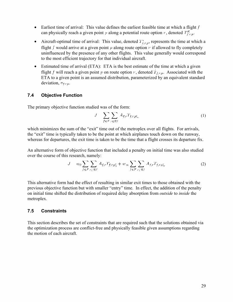
29

• Earliest time of arrival: This value defines the earliest feasible time at which a flight can physically reach a given point along a potential route option , denoted .

• Aircraft-optimal time of arrival: This value, denoted , represents the time at which a flight would arrive at a given point along route option if allowed to fly completely uninfluenced by the presence of any other flights. This value generally would correspond to the most efficient trajectory for that individual aircraft.

• Estimated time of arrival (ETA): ETA is the best estimate of the time at which a given flight will reach a given point on route option , denoted . Associated with the ETA to a given point is an assumed distribution, parameterized by an equivalent standard deviation, .

7.4 Objective Function The primary objective function studied was of the form:

(1)

which minimizes the sum of the “exit” time out of the metroplex over all flights. For arrivals, the “exit” time is typically taken to be the point at which airplanes touch down on the runway, whereas for departures, the exit time is taken to be the time that a flight crosses its departure fix. An alternative form of objective function that included a penalty on initial time was also studied over the course of this research, namely:

(2)

This alternative form had the effect of resulting in similar exit times to those obtained with the previous objective function but with smaller “entry” time. In effect, the addition of the penalty on initial time shifted the distribution of required delay absorption from outside to inside the metroplex.

7.5 Constraints This section describes the set of constraints that are required such that the solutions obtained via the optimization process are conflict-free and physically feasible given assumptions regarding the motion of each aircraft.

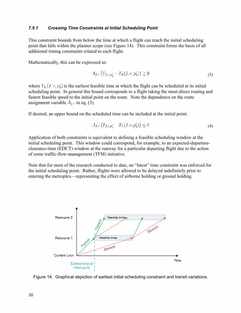
30

7.5.1 Crossing Time Constraints at Initial Scheduling Point

This constraint bounds from below the time at which a flight can reach the initial scheduling point that falls within the planner scope (see Figure 14). This constraint forms the basis of all additional timing constraints related to each flight. Mathematically, this can be expressed as:

(3)

where is the earliest feasible time at which the flight can be scheduled at its initial scheduling point. In general this bound corresponds to a flight taking the most-direct routing and fastest feasible speed to the initial point on the route. Note the dependence on the route assignment variable in eq. (3). If desired, an upper bound on the scheduled time can be included at the initial point:

(4)

Application of both constraints is equivalent to defining a feasible scheduling window at the initial scheduling point. This window could correspond, for example, to an expected-departure-clearance-time (EDCT) window at the runway for a particular departing flight due to the action of some traffic-flow-management (TFM) initiative. Note that for most of the research conducted to date, no “latest” time constraint was enforced for the initial scheduling point. Rather, flights were allowed to be delayed indefinitely prior to entering the metroplex—representing the effect of airborne holding or ground holding.

Figure 14. Graphical depiction of earliest initial scheduling constraint and transit variations.

31

7.5.2 Crossing Time Constraints at Final Scheduling Point

The formulation includes the ability to bound from above and below the time at which a flight must reach its final scheduling point within the planner scope, namely:

(5)

(6)

Such a constraint can be used to model a particular runway window for an arrival flight or, alternatively, a fix crossing time window for a departing flight. 7.5.3 Transit Time Constraints between Successive Scheduling Points

In order for the schedule obtained to be consistent with physical limitations of aircraft performance and air traffic operating procedures, constraints are introduced to bound from above and below the time for the aircraft to transition between two successive scheduling points on each of its potential route options:

(7)

(8)

7.5.4 Ordering Constraint at Potentially Shared Scheduling Points

For each pair of flights that can be assigned to routes that have at least one common point, the order at which the flights are to visit each of these shared points must be uniquely defined. Expressed in words: If:

• Flight is assigned to route : and

• Flight is assigned to route : , Then: for each scheduling point that is shared by routes and , either flight must be scheduled ahead of flight or vice versa, and can be expressed mathematically via the constraint:

(9)

Thus, the binary sequence indicator variables have only nonzero values when both of the corresponding pairs of route assignment variables are nonzero.

32

7.5.5 Separation Constraint at Potentially Shared Scheduling Points

Successive crossings of a given point by any pair of flights must often satisfy some separation constraint, which is often a function of some characteristic of each aircraft pair. Runway separation requirements due to wake vortex are an example of such a constraint. Expressed in words, this constraint is equivalent to the following set of conditions: If:

• Flight is assigned to route : and

• Flight is assigned to route : and

• Flight is sequenced ahead of at scheduling point , which is shared by routes and ,

Then: the scheduled crossing time of at point must be at least the minimum required separation seconds later than that of flight . Mathematically, this condition can be expressed by the constraint equation:

(10)

where one such inequality must be written for each potential ordering, for each pair of flights, at each potentially shared point.

7.6 Transformation to Linear Form Because of the dependence on route assignment, the objective function and the constraints defined in the previous sections involve a product of logical (binary) variables and/or a product of logical and continuous variables. In order to leverage open-source, self-contained mixed-integer-linear-program (MILP) solvers, it is necessary to transform the nonlinear constraints developed in the previous section into a set of equivalent linear constraints. 7.6.1 Product of Logical Variables

Each occurrence of a product of logical variables of the form can be replaced through the introduction of an auxiliary binary variable (Bemporad and Morari [20]):

(11)

Then, we append a set of auxiliary constraints:

(12)

33

7.6.2 Product of Logical and Continuous Variables

We can replace the occurrence of a product of logical and continuous variables of the form appearing in a constraint equation by replacing it with the auxiliary continuous variable (Bemporad and Morari [20]):

(13)

And appending the set of additional auxiliary constraints:

(14)

7.6.3 Summary of Linearized Mixed Integer Optimization Problem

Applying the linearization technique described previously results in the following MILP:

Objective: (15)

Initial condition: (16)

Minimum Transit: (17)

Maximum Transit: (18)

Ordering: (19)

Separation: (20)

Where the following variable substitutions have been made:

34

7.6.4 Alternate Linearized Form

It is possible to construct linear constraints using an alternative approach that reduces the number of binary variables required.

Objective Function

If we define a set of additional constraint equations:

(21)

where is a large positive constant value, then if is zero (e.g., flight is not assigned to route option ), then the scheduled time at all points on that route option will be forced to be zero, allowing us to rewrite the original nonlinear objective function expressed by eq. (1) in the linearized form:

(22)

Initial Scheduling Time Constraint

Consider the initial scheduling constraint given by eq. (3) and repeated here for convenience:

Effectively, this constraint expresses the statement: “If flight is assigned to route option , then the scheduled time at the first point on that route can be no earlier than .” An equivalent way to express this mathematically is:

(23)

If the value of is zero, the constraint is trivially satisfied given a sufficiently large positive constant, . Unlike the linearization technique given by eq. (13), the approach to linearization used in eq. (23) does not require the introduction of additional auxiliary constraint equations.

Transit Time Constraints

The transit-time constraints, repeated here:

can similarly be linearized through the introduction of a large positive constant:

(24)

(25)

35

Sequencing Constraint

The sequencing constraint at each potentially shared point (refer to eq. ... (9)) can equivalently be expressed via the pair of linear constraint equations:

(26)

(27)

Note the effect of the term scaling the difference in scheduled time. Consider the case where flight is assigned to route and flight is assigned to route , respectively. If the quantity in parenthesis is some positive value (thus implying that flight is scheduled before flight at shared point ), then eqs. (26) and (27) reduce to:

Since is a binary variable, then the only value that satisfies both constraints is unity.

Separation Constraint at Potentially Shared Nodes

The nonlinear separation constraint expressed in eq. (10) can alternatively be written as:

(28)

(29)

This pair of equations can be interpreted as follows: Consider first the case: .

Then, if is sequenced ahead of (e.g., ), the following must hold:

while eq. (29) is trivially satisfied. However, what if is sequenced ahead of ? In this case, eq. (28) is trivially satisfied and eq. (29) must hold:

If either or is zero, then both eqs. (28) and (29) are trivially satisfied as long as is larger than the separation value.

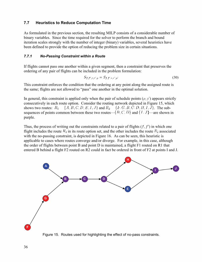
36

7.7 Heuristics to Reduce Computation Time As formulated in the previous section, the resulting MILP consists of a considerable number of binary variables. Since the time required for the solver to perform the branch and bound iteration scales strongly with the number of integer (binary) variables, several heuristics have been defined to provide the option of reducing the problem size in certain situations. 7.7.1 No-Passing Constraint within a Route

If flights cannot pass one another within a given segment, then a constraint that preserves the ordering of any pair of flights can be included in the problem formulation:

(30)

This constraint enforces the condition that the ordering at any point along the assigned route is the same; flights are not allowed to “pass” one another in the optimal solution. In general, this constraint is applied only when the pair of schedule points ( ) appears strictly consecutively in each route option. Consider the routing network depicted in Figure 15, which shows two routes: and . The sub-sequences of points common between these two routes— and —are shown in purple. Thus, the process of writing out the constraints related to a pair of flights ( ) in which one flight includes the route in its route option set, and the other includes the route associated with the no-passing constraint, is depicted in Figure 16. As can be seen, this heuristic is applicable to cases where routes converge and/or diverge. For example, in this case, although the order of flights between point B and point D is maintained, a flight F1 routed on R1 that entered B behind a flight F2 routed on R2 could in fact be ordered in front of F2 at points I and J.

Figure 15. Routes used for highlighting the effect of no-pass constraints.

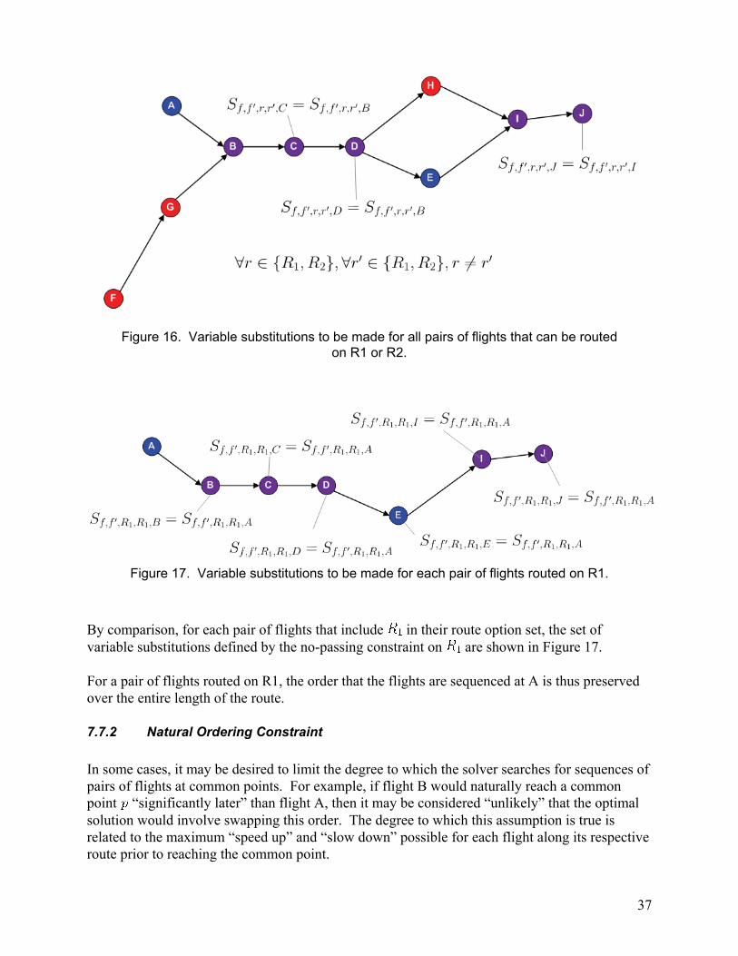
37

Figure 16. Variable substitutions to be made for all pairs of flights that can be routed on R1 or R2.

Figure 17. Variable substitutions to be made for each pair of flights routed on R1.

By comparison, for each pair of flights that include in their route option set, the set of variable substitutions defined by the no-passing constraint on are shown in Figure 17. For a pair of flights routed on R1, the order that the flights are sequenced at A is thus preserved over the entire length of the route. 7.7.2 Natural Ordering Constraint

In some cases, it may be desired to limit the degree to which the solver searches for sequences of pairs of flights at common points. For example, if flight B would naturally reach a common point “significantly later” than flight A, then it may be considered “unlikely” that the optimal solution would involve swapping this order. The degree to which this assumption is true is related to the maximum “speed up” and “slow down” possible for each flight along its respective route prior to reaching the common point.

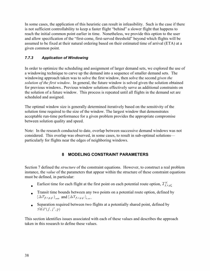
38

In some cases, the application of this heuristic can result in infeasibility. Such is the case if there is not sufficient controllability to keep a faster flight “behind” a slower flight that happens to reach the initial common point earlier in time. Nonetheless, we provide this option to the user and allow specification of the “first-come, first-served threshold” beyond which flights will be assumed to be fixed at their natural ordering based on their estimated time of arrival (ETA) at a given common point. 7.7.3 Application of Windowing

In order to optimize the scheduling and assignment of larger demand sets, we explored the use of a windowing technique to carve up the demand into a sequence of smaller demand sets. The windowing approach taken was to solve the first window, then solve the second given the solution of the first window. In general, the future window is solved given the solution obtained for previous windows.. Previous window solutions effectively serve as additional constraints on the solution of a future window. This process is repeated until all flights in the demand set are scheduled and assigned. The optimal window size is generally determined iteratively based on the sensitivity of the solution time required to the size of the window. The largest window that demonstrates acceptable run-time performance for a given problem provides the appropriate compromise between solution quality and speed. Note: In the research conducted to date, overlap between successive demand windows was not considered. This overlap was observed, in some cases, to result in sub-optimal solutions—particularly for flights near the edges of neighboring windows.

8 MODELING CONSTRAINT PARAMETERS

Section 7 defined the structure of the constraint equations. However, to construct a real problem instance, the value of the parameters that appear within the structure of these constraint equations must be defined, in particular:

• Earliest time for each flight at the first point on each potential route option,

• Transit time bounds between any two points on a potential route option, defined by and

• Separation required between two flights at a potentially shared point, defined by

This section identifies issues associated with each of these values and describes the approach taken in this research to define these values.

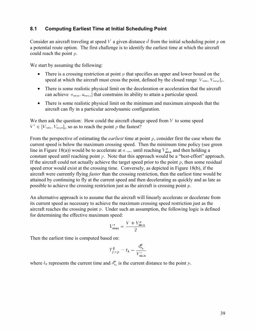
39

8.1 Computing Earliest Time at Initial Scheduling Point Consider an aircraft traveling at speed a given distance from the initial scheduling point on a potential route option. The first challenge is to identify the earliest time at which the aircraft could reach the point . We start by assuming the following:

• There is a crossing restriction at point that specifies an upper and lower bound on the speed at which the aircraft must cross the point, defined by the closed range .

• There is some realistic physical limit on the deceleration or acceleration that the aircraft can achieve that constrains its ability to attain a particular speed.

• There is some realistic physical limit on the minimum and maximum airspeeds that the aircraft can fly in a particular aerodynamic configuration.

We then ask the question: How could the aircraft change speed from to some speed

so as to reach the point the fastest? From the perspective of estimating the earliest time at point , consider first the case where the current speed is below the maximum crossing speed. Then the minimum time policy (see green line in Figure 18(a)) would be to accelerate at until reaching and then holding a constant speed until reaching point . Note that this approach would be a “best-effort” approach. If the aircraft could not actually achieve the target speed prior to the point , then some residual speed error would exist at the crossing time. Conversely, as depicted in Figure 18(b), if the aircraft were currently flying faster than the crossing restriction, then the earliest time would be attained by continuing to fly at the current speed and then decelerating as quickly and as late as possible to achieve the crossing restriction just as the aircraft is crossing point . An alternative approach is to assume that the aircraft will linearly accelerate or decelerate from its current speed as necessary to achieve the maximum crossing speed restriction just as the aircraft reaches the crossing point . Under such an assumption, the following logic is defined for determining the effective maximum speed:

Then the earliest time is computed based on:

where represents the current time and is the current distance to the point .

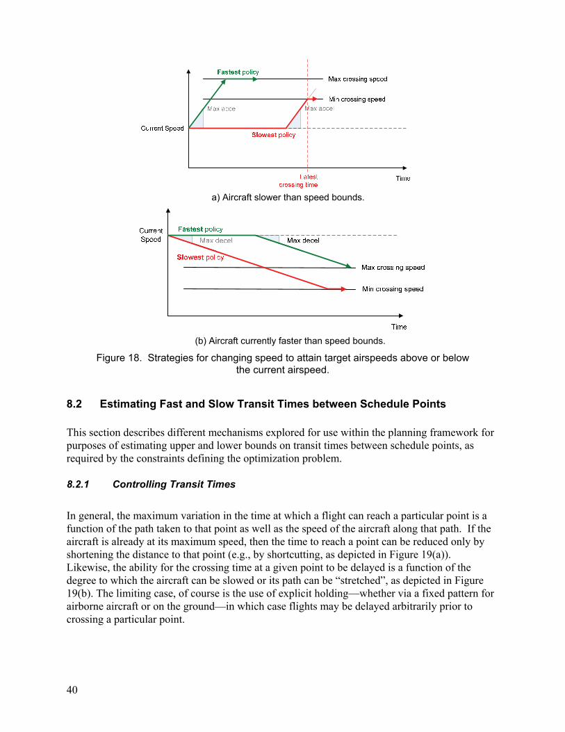
40

a) Aircraft slower than speed bounds.

(b) Aircraft currently faster than speed bounds.

Figure 18. Strategies for changing speed to attain target airspeeds above or below the current airspeed.

8.2 Estimating Fast and Slow Transit Times between Schedule Points This section describes different mechanisms explored for use within the planning framework for purposes of estimating upper and lower bounds on transit times between schedule points, as required by the constraints defining the optimization problem. 8.2.1 Controlling Transit Times

In general, the maximum variation in the time at which a flight can reach a particular point is a function of the path taken to that point as well as the speed of the aircraft along that path. If the aircraft is already at its maximum speed, then the time to reach a point can be reduced only by shortening the distance to that point (e.g., by shortcutting, as depicted in Figure 19(a)). Likewise, the ability for the crossing time at a given point to be delayed is a function of the degree to which the aircraft can be slowed or its path can be “stretched”, as depicted in Figure 19(b). The limiting case, of course is the use of explicit holding—whether via a fixed pattern for airborne aircraft or on the ground—in which case flights may be delayed arbitrarily prior to crossing a particular point.

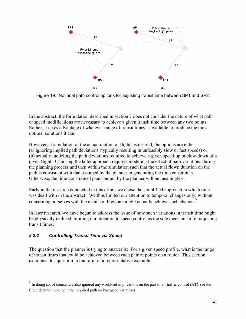
41

Figure 19. Notional path control options for adjusting transit time between SP1 and SP2.

In the abstract, the formulation described in section 7 does not consider the nature of what path or speed modifications are necessary to achieve a given transit time between any two points. Rather, it takes advantage of whatever range of transit times is available to produce the most optimal solutions it can. However, if simulation of the actual motion of flights is desired, the options are either (a) ignoring implied path deviations (typically resulting in unfeasibly slow or fast speeds) or (b) actually modeling the path deviations required to achieve a given speed-up or slow-down of a given flight. Choosing the latter approach requires modeling the effect of path variations during the planning process and then within the simulation such that the actual flown duration on the path is consistent with that assumed by the planner in generating the time constraints. Otherwise, the time-constrained plans output by the planner will be meaningless. Early in the research conducted in this effort, we chose the simplified approach in which time was dealt with in the abstract. We thus limited our attention to temporal changes only, without concerning ourselves with the details of how one might actually achieve such changes

5.

In later research, we have begun to address the issue of how such variations in transit time might be physically realized, limiting our attention to speed control as the sole mechanism for adjusting transit times. 8.2.2 Controlling Transit Time via Speed

The question that the planner is trying to answer is: For a given speed profile, what is the range of transit times that could be achieved between each pair of points on a route? This section examines this question in the form of a representative example.

5 In doing so, of course, we also ignored any workload implications on the part of air traffic control (ATC) or the

flight deck to implement the required path and/or speed variations.

42

Consider a route consisting of three schedule points (A,B,C) as depicted in Figure 20. At each point, we assume the specification of a speed crossing restriction, expressed as a fastest and slowest speed at which aircraft can cross the point. In current operations, these speed restrictions might model the action of controllers to manage speeds within the terminal area. It is further assumed that these speed restrictions are “within” the physical speed limitations of aircraft maneuvering along a given route—and thus can feasibly be obtained by the aircraft. Given this route and assumed speed profile, the objective in this section is then to explore the range of upper and lower bounds on transit time achievable between successive schedule points. Mathematically, if we assume a constant acceleration (which may be zero), then the transit time between any two points is defined by the ratio of the distance between the points and the average speed:

(31)

The first question to answer is the nature of the aircraft speed along a given segment. Should it be modeled as a constant speed or involve some acceleration or deceleration?

0 5 10 15 20 25 30 35 40120

140

160

180

200

220

240

260

Distance to touchdown [nmi]

Spe

ed [

knot

s]

Figure 20. Representative speed profile specification along a route.

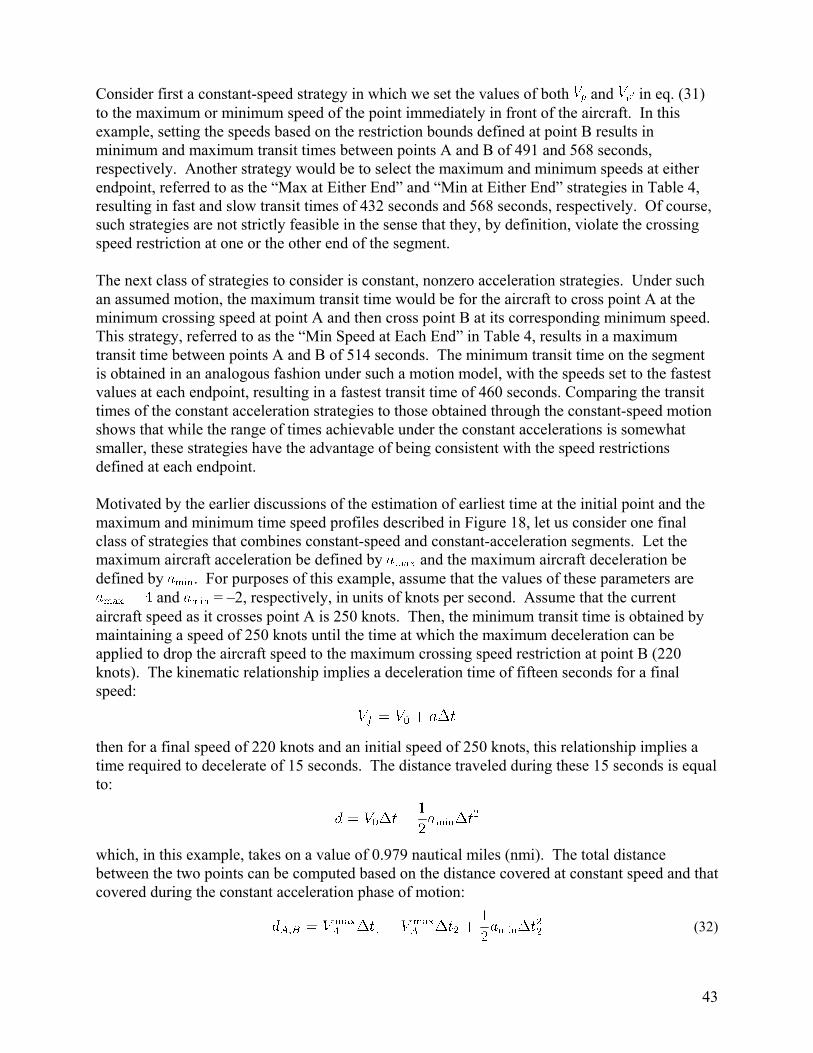
43

Consider first a constant-speed strategy in which we set the values of both and in eq. (31) to the maximum or minimum speed of the point immediately in front of the aircraft. In this example, setting the speeds based on the restriction bounds defined at point B results in minimum and maximum transit times between points A and B of 491 and 568 seconds, respectively. Another strategy would be to select the maximum and minimum speeds at either endpoint, referred to as the “Max at Either End” and “Min at Either End” strategies in Table 4, resulting in fast and slow transit times of 432 seconds and 568 seconds, respectively. Of course, such strategies are not strictly feasible in the sense that they, by definition, violate the crossing speed restriction at one or the other end of the segment. The next class of strategies to consider is constant, nonzero acceleration strategies. Under such an assumed motion, the maximum transit time would be for the aircraft to cross point A at the minimum crossing speed at point A and then cross point B at its corresponding minimum speed. This strategy, referred to as the “Min Speed at Each End” in Table 4, results in a maximum transit time between points A and B of 514 seconds. The minimum transit time on the segment is obtained in an analogous fashion under such a motion model, with the speeds set to the fastest values at each endpoint, resulting in a fastest transit time of 460 seconds. Comparing the transit times of the constant acceleration strategies to those obtained through the constant-speed motion shows that while the range of times achievable under the constant accelerations is somewhat smaller, these strategies have the advantage of being consistent with the speed restrictions defined at each endpoint. Motivated by the earlier discussions of the estimation of earliest time at the initial point and the maximum and minimum time speed profiles described in Figure 18, let us consider one final class of strategies that combines constant-speed and constant-acceleration segments. Let the maximum aircraft acceleration be defined by and the maximum aircraft deceleration be defined by . For purposes of this example, assume that the values of these parameters are

and = –2, respectively, in units of knots per second. Assume that the current aircraft speed as it crosses point A is 250 knots. Then, the minimum transit time is obtained by maintaining a speed of 250 knots until the time at which the maximum deceleration can be applied to drop the aircraft speed to the maximum crossing speed restriction at point B (220 knots). The kinematic relationship implies a deceleration time of fifteen seconds for a final speed:

then for a final speed of 220 knots and an initial speed of 250 knots, this relationship implies a time required to decelerate of 15 seconds. The distance traveled during these 15 seconds is equal to:

which, in this example, takes on a value of 0.979 nautical miles (nmi). The total distance between the two points can be computed based on the distance covered at constant speed and that covered during the constant acceleration phase of motion:

(32)

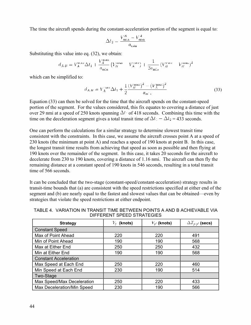
44

The time the aircraft spends during the constant-acceleration portion of the segment is equal to:

Substituting this value into eq. (32), we obtain:

which can be simplified to:

(33)

Equation (33) can then be solved for the time that the aircraft spends on the constant-speed portion of the segment. For the values considered, this fix equates to covering a distance of just over 29 nmi at a speed of 250 knots spanning of 418 seconds. Combining this time with the time on the deceleration segment gives a total transit time of = 433 seconds. One can perform the calculations for a similar strategy to determine slowest transit time consistent with the constraints. In this case, we assume the aircraft crosses point A at a speed of 230 knots (the minimum at point A) and reaches a speed of 190 knots at point B. In this case, the longest transit time results from achieving that speed as soon as possible and then flying at 190 knots over the remainder of the segment. In this case, it takes 20 seconds for the aircraft to decelerate from 230 to 190 knots, covering a distance of 1.16 nmi. The aircraft can then fly the remaining distance at a constant speed of 190 knots in 546 seconds, resulting in a total transit time of 566 seconds. It can be concluded that the two-stage (constant-speed/constant-acceleration) strategy results in transit-time bounds that (a) are consistent with the speed restrictions specified at either end of the segment and (b) are nearly equal to the fastest and slowest values that can be obtained—even by strategies that violate the speed restrictions at either endpoint.

TABLE 4. VARIATION IN TRANSIT TIME BETWEEN POINTS A AND B ACHIEVABLE VIA DIFFERENT SPEED STRATEGIES

Strategy (knots) (knots) (secs)

Constant Speed Max of Point Ahead 220 220 491 Min of Point Ahead 190 190 568 Max at Either End 250 250 432 Min at Either End 190 190 568 Constant Acceleration Max Speed at Each End 250 220 460 Min Speed at Each End 230 190 514 Two-Stage Max Speed/Max Deceleration 250 220 433 Max Deceleration/Min Speed 230 190 566

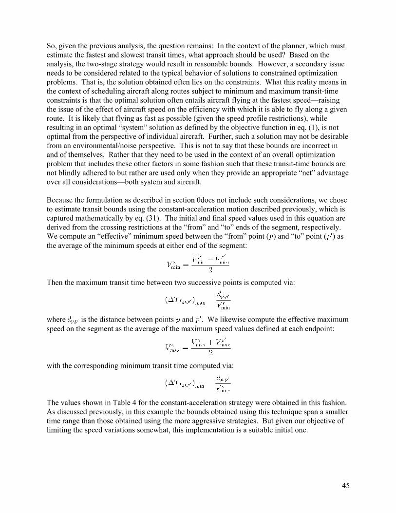
45

So, given the previous analysis, the question remains: In the context of the planner, which must estimate the fastest and slowest transit times, what approach should be used? Based on the analysis, the two-stage strategy would result in reasonable bounds. However, a secondary issue needs to be considered related to the typical behavior of solutions to constrained optimization problems. That is, the solution obtained often lies on the constraints. What this reality means in the context of scheduling aircraft along routes subject to minimum and maximum transit-time constraints is that the optimal solution often entails aircraft flying at the fastest speed—raising the issue of the effect of aircraft speed on the efficiency with which it is able to fly along a given route. It is likely that flying as fast as possible (given the speed profile restrictions), while resulting in an optimal “system” solution as defined by the objective function in eq. (1), is not optimal from the perspective of individual aircraft. Further, such a solution may not be desirable from an environmental/noise perspective. This is not to say that these bounds are incorrect in and of themselves. Rather that they need to be used in the context of an overall optimization problem that includes these other factors in some fashion such that these transit-time bounds are not blindly adhered to but rather are used only when they provide an appropriate “net” advantage over all considerations—both system and aircraft. Because the formulation as described in section 0does not include such considerations, we chose to estimate transit bounds using the constant-acceleration motion described previously, which is captured mathematically by eq. (31). The initial and final speed values used in this equation are derived from the crossing restrictions at the “from” and “to” ends of the segment, respectively. We compute an “effective” minimum speed between the “from” point ( ) and “to” point ( ) as the average of the minimum speeds at either end of the segment:

Then the maximum transit time between two successive points is computed via:

where is the distance between points and . We likewise compute the effective maximum speed on the segment as the average of the maximum speed values defined at each endpoint:

with the corresponding minimum transit time computed via:

The values shown in Table 4 for the constant-acceleration strategy were obtained in this fashion. As discussed previously, in this example the bounds obtained using this technique span a smaller time range than those obtained using the more aggressive strategies. But given our objective of limiting the speed variations somewhat, this implementation is a suitable initial one.

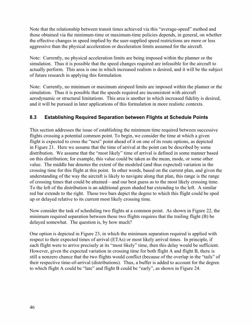
46

Note that the relationship between transit times achieved via this “average-speed” method and those obtained via the minimum-time or maximum-time policies depends, in general, on whether the effective changes in speed implied by the user-supplied speed restrictions are more or less aggressive than the physical acceleration or deceleration limits assumed for the aircraft. Note: Currently, no physical acceleration limits are being imposed within the planner or the simulation. Thus it is possible that the speed changes required are infeasible for the aircraft to actually perform. This area is one in which increased realism is desired, and it will be the subject of future research in applying this formulation. Note: Currently, no minimum or maximum airspeed limits are imposed within the planner or the simulation. Thus it is possible that the speeds required are inconsistent with aircraft aerodynamic or structural limitations. This area is another in which increased fidelity is desired, and it will be pursued in later applications of this formulation in more realistic contexts.

8.3 Establishing Required Separation between Flights at Schedule Points This section addresses the issue of establishing the minimum time required between successive flights crossing a potential common point. To begin, we consider the time at which a given flight is expected to cross the “next” point ahead of it on one of its route options, as depicted in Figure 21. Here we assume that the time of arrival at the point can be described by some distribution. We assume that the “most likely” time of arrival is defined in some manner based on this distribution; for example, this value could be taken as the mean, mode, or some other value. The middle bar denotes the extent of the modeled (and thus expected) variation in the crossing time for this flight at this point. In other words, based on the current plan, and given the understanding of the way the aircraft is likely to navigate along that plan, this range is the range of crossing times that could be attained—and our best guess as to the most likely crossing time. To the left of the distribution is an additional green shaded bar extending to the left. A similar red bar extends to the right. These two bars depict the degree to which this flight could be sped up or delayed relative to its current most likely crossing time. Now consider the task of scheduling two flights at a common point. As shown in Figure 22, the minimum required separation between these two flights requires that the trailing flight (B) be delayed somewhat. The question is, by how much? One option is depicted in Figure 23, in which the minimum separation required is applied with respect to their expected times of arrival (ETAs) or most likely arrival times. In principle, if each flight were to arrive precisely at its “most likely” time, then this delay would be sufficient. However, given the expected variation in crossing time for both flight A and flight B, there is still a nonzero chance that the two flights would conflict (because of the overlap in the “tails” of their respective time-of-arrival (distributions). Thus, a buffer is added to account for the degree to which flight A could be “late” and flight B could be “early”, as shown in Figure 24.

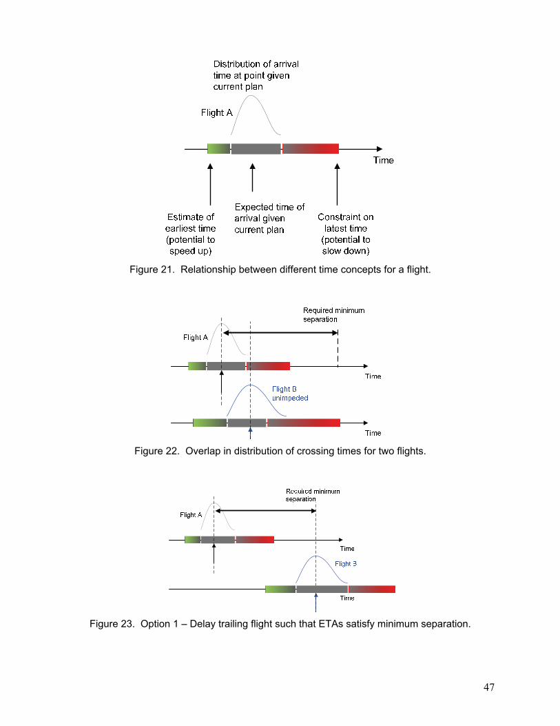
47

Figure 21. Relationship between different time concepts for a flight.

Figure 22. Overlap in distribution of crossing times for two flights.

Figure 23. Option 1 – Delay trailing flight such that ETAs satisfy minimum separation.

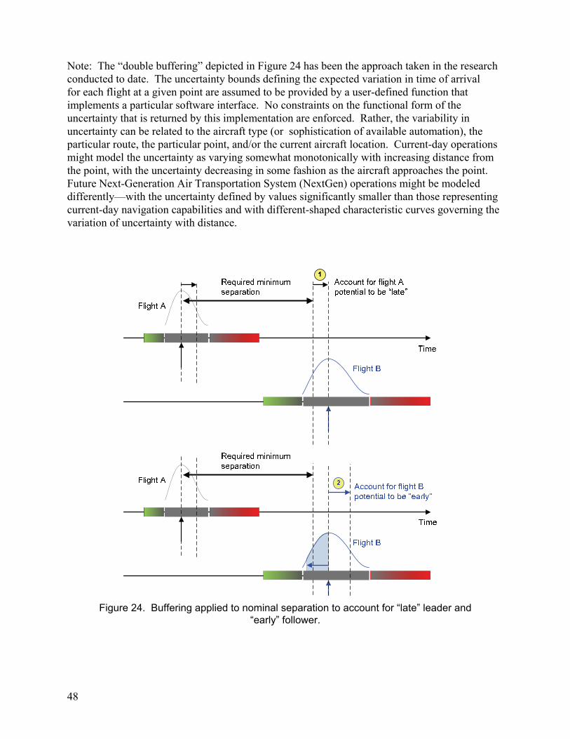
48

Note: The “double buffering” depicted in Figure 24 has been the approach taken in the research conducted to date. The uncertainty bounds defining the expected variation in time of arrival for each flight at a given point are assumed to be provided by a user-defined function that implements a particular software interface. No constraints on the functional form of the uncertainty that is returned by this implementation are enforced. Rather, the variability in uncertainty can be related to the aircraft type (or sophistication of available automation), the particular route, the particular point, and/or the current aircraft location. Current-day operations might model the uncertainty as varying somewhat monotonically with increasing distance from the point, with the uncertainty decreasing in some fashion as the aircraft approaches the point. Future Next-Generation Air Transportation System (NextGen) operations might be modeled differently—with the uncertainty defined by values significantly smaller than those representing current-day navigation capabilities and with different-shaped characteristic curves governing the variation of uncertainty with distance.

Figure 24. Buffering applied to nominal separation to account for “late” leader and “early” follower.

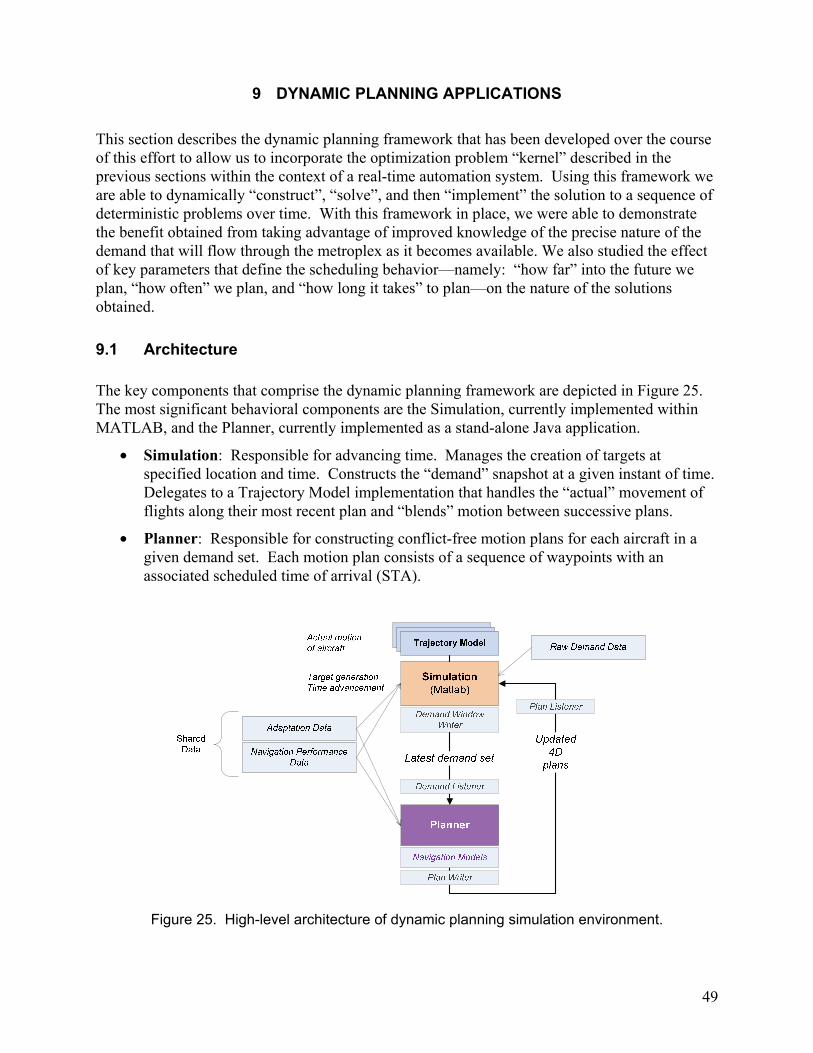
49

9 DYNAMIC PLANNING APPLICATIONS

This section describes the dynamic planning framework that has been developed over the course of this effort to allow us to incorporate the optimization problem “kernel” described in the previous sections within the context of a real-time automation system. Using this framework we are able to dynamically “construct”, “solve”, and then “implement” the solution to a sequence of deterministic problems over time. With this framework in place, we were able to demonstrate the benefit obtained from taking advantage of improved knowledge of the precise nature of the demand that will flow through the metroplex as it becomes available. We also studied the effect of key parameters that define the scheduling behavior—namely: “how far” into the future we plan, “how often” we plan, and “how long it takes” to plan—on the nature of the solutions obtained.

9.1 Architecture The key components that comprise the dynamic planning framework are depicted in Figure 25. The most significant behavioral components are the Simulation, currently implemented within MATLAB, and the Planner, currently implemented as a stand-alone Java application.

• Simulation: Responsible for advancing time. Manages the creation of targets at specified location and time. Constructs the “demand” snapshot at a given instant of time. Delegates to a Trajectory Model implementation that handles the “actual” movement of flights along their most recent plan and “blends” motion between successive plans.

• Planner: Responsible for constructing conflict-free motion plans for each aircraft in a given demand set. Each motion plan consists of a sequence of waypoints with an associated scheduled time of arrival (STA).

Figure 25. High-level architecture of dynamic planning simulation environment.

50

The interprocess communication used to synchronize these two processes is the local file system. The Planner application includes a “Demand Listener”, which listens for updates to a specific file (LatestDemandSet.xml). Upon detecting an update, this listener sends an event to the Planner triggering a planning cycle. The Simulation includes an analogous “Plan Listener” that detects when plans are available to be “implemented” within the simulation. 9.1.1 Greedy First-Come, First-Served Planner

As an alternative to the mixed-integer-linear-program (MILP) planner—both to provide an analytical reference and to demonstrate the plug-and-play dynamic planning framework developed under this effort—we have implemented a “greedy” first-come, first-served (FCFS) planner. The greedy FCFS planner sorts the flights within a given demand set in the order of their earliest time at their initial scheduling point. It then processes each flight in turn, searching over all route options to find the route at which the flight can be scheduled that minimizes its scheduled time at its final scheduling point. As such, the objective function used within the greedy FCFS planner is analogous to the “final time” objective defined for the MILP planner. As the greedy FCFS planner attempts to schedule a given flight on a potential resource, it accounts for the resource usage associated with any previously scheduled flights on that resource, complying with the separation requirement. It should be noted that the greedy FCFS planner utilizes the same uncertainty model with respect to time-of-arrival behavior. Thus, the interflight spacing defined within the greedy FCFS planner is consistent with that applied by the MILP planner for the same pair of flights. The greedy FCFS planner also leverages the same “earliest” and “latest” time calculations such that transit times are consistent with the MILP planner. As such, plans generated by the greedy FCFS planner can be directly compared with those output by the MILP planner for a given demand set.

9.2 Interfaces between Simulation and Planner The inputs required by the Planner to construct a plan are: (a) the demand set, (b) the set of routes defined for the planning cycle with associated speed profiles, (c) the set of schedule points defined for the planning cycle with associated separation rules, and (d) the expected variation in time-of-arrival behavior. 9.2.1 Demand-Set Description

Each demand set, which is tagged with the simulation time at which the “snapshot” was taken, consists of the following information for each flight:

• Unique flight identifier

• Current position (expressed as nautical miles east and north of metroplex “center”)

• Current altitude (feet mean sea level (MSL))

• Current ground course (degrees relative to true north)

• Current ground speed (knots)

• Origin airport

51

• Destination airport

• Type (used for mapping to separation rules and time-of-arrival behavior)

• Category (arrival or departure)

• Cardinal direction from which the aircraft is approaching the metroplex (e.g., E, NE, S)

• Earliest gate departure pushback time (secs) 9.2.2 Route Description

The routing network that exists at the start of each planning cycle must define:

• The set of airports within the metroplex

• The set of runways available at each airport

• The set of fixes

• Any waypoints, not including runway endpoints or fixes

• The set of routes, each of which must include a fix and runway 9.2.3 Scheduling-Point Description

The input data for the planner must also include a specification of the points at which separation rules are to be enforced by the schedule. Each scheduling point includes:

• The name of the point, which must be the name of a fix, runway, or waypoint defined as part of the route description

• The minimum required separation at that point, specified as a number of seconds by which the “trailer” must follow the “leader” at that point

• Optionally, defining of aircraft type-specific rules that provide a separation that is a function of the “leader” and “trailer” type (see section 0)

9.2.4 Expected Time-of-Arrival Behavior

As described in section 0, time-of-arrival behavior is parameterized in the form of a standard deviation about the nominal time of an aircraft. This value is obtained by calling out on a well-defined software interface to a user-specified implementation. The current default implementation provides an uncertainty value (which is assumed to represent the 1- of the underlying distribution) that increases with increasing distance from the point, as depicted in Figure 26. This model outputs an uncertainty value that decreases linearly to zero as the distance to the point goes to zero. The uncertainty value maxes out at a value of 300 seconds for aircraft more than 100 nmi from a given point. It should be noted that this model is not intended to be realistic—rather it is solely a starting point for analysis. By implementing the required software interface, users can provide an uncertainty model that is best suited for a given scenario.

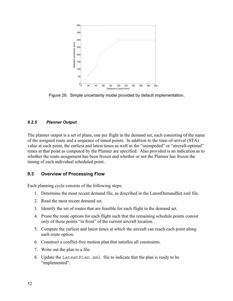
52

Figure 26. Simple uncertainty model provided by default implementation.

9.2.5 Planner Output

The planner output is a set of plans, one per flight in the demand set, each consisting of the name of the assigned route and a sequence of timed points. In addition to the time-of-arrival (STA) value at each point, the earliest and latest times as well as the “unimpeded” or “aircraft-optimal” times at that point as computed by the Planner are specified. Also provided is an indication as to whether the route assignment has been frozen and whether or not the Planner has frozen the timing of each individual scheduled point.

9.3 Overview of Processing Flow Each planning cycle consists of the following steps:

1. Determine the most recent demand file, as described in the LatestDemandSet.xml file.

2. Read the most recent demand set.

3. Identify the set of routes that are feasible for each flight in the demand set.

4. Prune the route options for each flight such that the remaining schedule points consist only of those points “in front” of the current aircraft location.

5. Compute the earliest and latest times at which the aircraft can reach each point along each route option.

6. Construct a conflict-free motion plan that satisfies all constraints.

7. Write out the plan to a file.

8. Update the LatestPlan.xml file to indicate that the plan is ready to be “implemented”.

0 20 40 60 80 100 120 140 160 180 2000

50

100

150

200

250

300

350

400

Distance to point [nmi]

Mod

eled

unc

erta

inty

[se

c]

53

The Simulation, which is itself blocked while the Planner is computing a given plan, incorporates a PlanListener that then detects the update of the LatestPlan.xml file. In response, the Simulation then reads in the updated plan and distributes the individual time-based routes to each aircraft modeled within the simulation. The Trajectory Model for each aircraft, upon receipt of a new route, prunes the route to keep only those points that are physically and temporally “in front of” the aircraft at the time the plan is received. The Trajectory Model then performs a calculation to update its target speed to comply with the STA at the point immediately in front of it. Specifically it computes the distance between the current location of the aircraft and its next schedule point, , as well as the time available to reach that point:

(34)

Within the Trajectory Model, a low-pass filter with a 10-second time constant is utilized to generate the actual aircraft speed in tracking to the commanded speed. Currently, no “error” is introduced within the “actual” trajectory model—other than the time response implied by the low-pass filter. Rather, each aircraft generally crosses each schedule point at the most recent STA defined at that point. This modeling was done so that we could separately study the effect of demand uncertainty from execution uncertainty.

9.4 Control of Time The interaction between the Simulation and Planner occurs in a lock-step fashion, with the Simulation responsible for advancing time forward. Controlling time in this manner allows us to model and study the effect of different computational times without actually having to achieve that computation time. At a high level, the flow of execution is described by the following sequence:

1. Simulation advances time to the start of the next planning cycle (Plan ). Trajectory Model moves aircraft according to Plan .

2. Simulation advances time to the point at which Plan is available for implementation, modeled via the parameter PlanComputationSecs, allowing us to study the effect of different computational times required to solve a given problem instance.

3. Simulation constructs the demand set based on the current location of all aircraft, and including flights that will be active between the current time and PlanHorizonSecs into the future. Simulation writes out the demand set and updates the content of the LatestDemandSet.xml file to identify the file containing the data.

4. Simulation blocks [[blocks what? flights?]], awaiting for event indicating that Plan is ready for implementation.

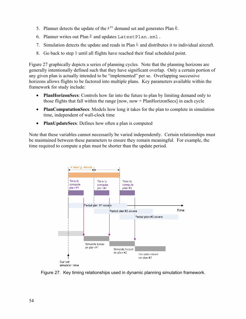
54

5. Planner detects the update of the demand set and generates Plan .

6. Planner writes out Plan and updates LatestPlan.xml.

7. Simulation detects the update and reads in Plan and distributes it to individual aircraft.

8. Go back to step 1 until all flights have reached their final scheduled point. Figure 27 graphically depicts a series of planning cycles. Note that the planning horizons are generally intentionally defined such that they have significant overlap. Only a certain portion of any given plan is actually intended to be “implemented” per se. Overlapping successive horizons allows flights to be factored into multiple plans. Key parameters available within the framework for study include:

• PlanHorizonSecs: Controls how far into the future to plan by limiting demand only to those flights that fall within the range [now, now + PlanHorizonSecs] in each cycle

• PlanComputationSecs: Models how long it takes for the plan to complete in simulation time, independent of wall-clock time

• PlanUpdateSecs: Defines how often a plan is computed Note that these variables cannot necessarily be varied independently. Certain relationships must be maintained between these parameters to ensure they remain meaningful. For example, the time required to compute a plan must be shorter than the update period.

Figure 27. Key timing relationships used in dynamic planning simulation framework.

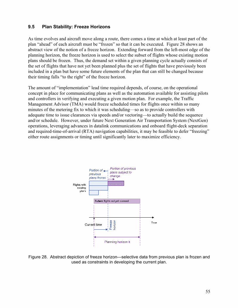
55

9.5 Plan Stability: Freeze Horizons As time evolves and aircraft move along a route, there comes a time at which at least part of the plan “ahead” of each aircraft must be “frozen” so that it can be executed. Figure 28 shows an abstract view of the notion of a freeze horizon. Extending forward from the left-most edge of the planning horizon, the freeze horizon is used to select the subset of flights whose existing motion plans should be frozen. Thus, the demand set within a given planning cycle actually consists of the set of flights that have not yet been planned plus the set of flights that have previously been included in a plan but have some future elements of the plan that can still be changed because their timing falls “to the right” of the freeze horizon. The amount of “implementation” lead time required depends, of course, on the operational concept in place for communicating plans as well as the automation available for assisting pilots and controllers in verifying and executing a given motion plan. For example, the Traffic Management Advisor (TMA) would freeze scheduled times for flights once within so many minutes of the metering fix to which it was scheduling—so as to provide controllers with adequate time to issue clearances via speeds and/or vectoring—to actually build the sequence and/or schedule. However, under future Next Generation Air Transportation System (NextGen) operations, leveraging advances in datalink communications and onboard flight-deck separation and required-time-of-arrival (RTA) navigation capabilities, it may be feasible to defer “freezing” either route assignments or timing until significantly later to maximize efficiency.

Figure 28. Abstract depiction of freeze horizon—selective data from previous plan is frozen and used as constraints in developing the current plan.

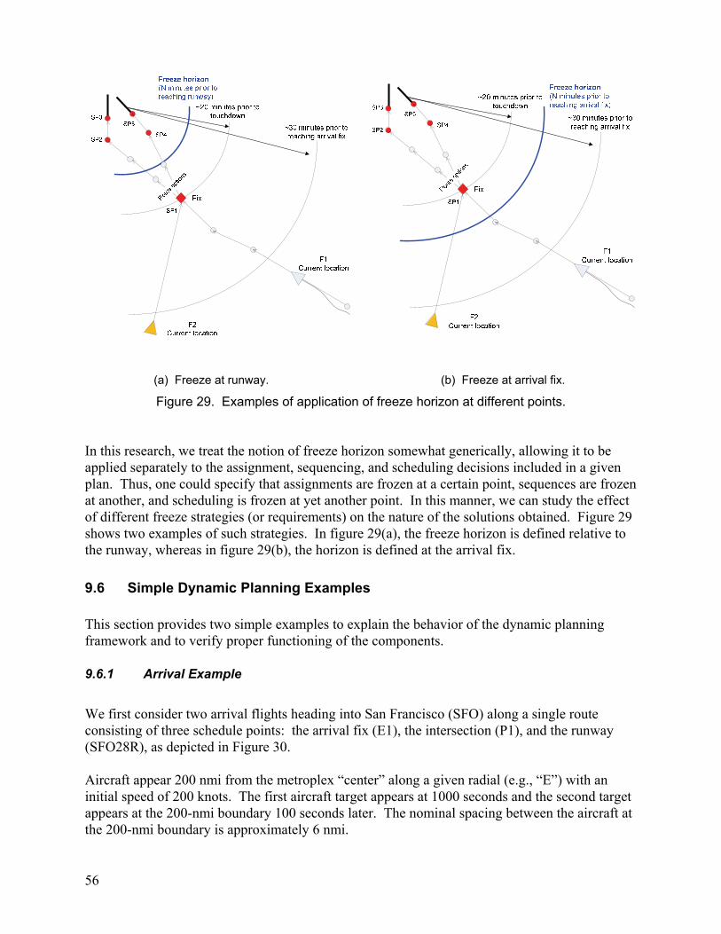
56

(a) Freeze at runway. (b) Freeze at arrival fix.

Figure 29. Examples of application of freeze horizon at different points. In this research, we treat the notion of freeze horizon somewhat generically, allowing it to be applied separately to the assignment, sequencing, and scheduling decisions included in a given plan. Thus, one could specify that assignments are frozen at a certain point, sequences are frozen at another, and scheduling is frozen at yet another point. In this manner, we can study the effect of different freeze strategies (or requirements) on the nature of the solutions obtained. Figure 29 shows two examples of such strategies. In figure 29(a), the freeze horizon is defined relative to the runway, whereas in figure 29(b), the horizon is defined at the arrival fix.

9.6 Simple Dynamic Planning Examples This section provides two simple examples to explain the behavior of the dynamic planning framework and to verify proper functioning of the components. 9.6.1 Arrival Example

We first consider two arrival flights heading into San Francisco (SFO) along a single route consisting of three schedule points: the arrival fix (E1), the intersection (P1), and the runway (SFO28R), as depicted in Figure 30. Aircraft appear 200 nmi from the metroplex “center” along a given radial (e.g., “E”) with an initial speed of 200 knots. The first aircraft target appears at 1000 seconds and the second target appears at the 200-nmi boundary 100 seconds later. The nominal spacing between the aircraft at the 200-nmi boundary is approximately 6 nmi.

57

Figure 30. Simple arrival scenario.

The minimum required separation at the points along the route is defined to be 60 seconds at the runway (SFO28R) and 90 seconds at the intersection P1 and fix E1. The model governing the time-of-arrival uncertainty is that depicted in Figure 26. Running the framework on this example results in the “time-of-arrival” graphic depicted in Figure 31 at the arrival fix E1. In this graphic simulation time is plotted on the x-axis while various values of the crossing time at the point E1 are plotted on the y-axis. Notionally, this plot allows one to analyze the evolution in various aspects of the crossing time for each flight in time as influenced by the periodic plan updates. For each flight four “lines” are included:

• The red lines (with diamonds) depict the latest crossing time for each flight as computed at the beginning of each planning cycle.

• The green lines (with asterisks) depict the earliest crossing time for each flight as computed at the beginning of each planning cycle.

• The blue line (with circles) depicts the scheduled crossing time for each flight as computed by the Planner and output at the end of each planning cycle.

• The black dashed lines depict the actual crossing time for each flight as generated by the Trajectory Model within the Simulation.

Several observations regarding this graphic can be made. First, notice that the sequence of STA values for the “leader” flight, FA1, ride along the earliest feasible time line at each planning cycle. Second, notice that the “follower” STA values lie above the “latest time” line for FA2, a consequence of the fact that the “latest time” computation accounts only for delays related to speed control.

-100 -50 0 50 100 150 200

-100

-80

-60

-40

-20

0

20

40

60

80

100

P1 E1 FA1

Current time secs: 1300

FA2

Distance east of center [nmi]

Dis

tanc

e no

rth

of c

ente

r [n

mi

SFO28R

Speed restrictions at E1

[250,270]

@P1: [200,220]

@SFO28R:

[120,120]

58

1000 1500 2000 2500 3000 3500

3000

3200

3400

3600

3800

4000

4200

FA1 STA

FA1 ATA

Arrivals approaching E1

Time into simulation [sec]

Cro

ssin

g tim

e at

poi

nt [

sec]

FA2 STA

FA2 ATA

Figure 31. Representative time-of-arrival graphic at the fix E1.

As described in section 0, in this case no upper bound was placed on the scheduled time at the initial schedule point (E1). Thus, some other form of control—through path stretching or holding—would be necessary to absorb the delay implied by Figure 31. A third observation can be made regarding the vertical distance between the STA lines for FA1 and FA2. At the end of the first planning cycle, when both aircraft are on the order of 200 nmi away from point E1, the separation enforced by the plan is approximately 700 seconds. Recall that the minimum required separation is 90 seconds. The excess padding is a result of the modeled uncertainty, which, based on Figure 26, is on the order of 300 seconds per flight. However, as the flights progress toward the arrival fix, note how the distance between the STA lines gets smaller, reaching a minimum value of 500 seconds as flight FA1 crosses point E1. Note that by the start of the planning cycle at 3100 seconds, flight FA2 is flying along the fastest speed bound. At this point, as depicted in Figure 32, the flight FA2 is ~40 nmi from E1. As such, the required separation between the flights is 90 seconds plus that due to uncertainty, which is on the order of 100 seconds. Thus, only approximately 200 seconds is strictly required. However, since by this point FA2 is flying almost as fast as it can on this segment (as limited by the crossing speed restrictions at point E1), it is unable to make up any further distance prior to reaching E1. Figure 33 shows the variation of the actual speed as determined by the Trajectory Model for each aircraft during this simulation. Here the convergence of the leader FA1 to its fastest speed is apparent as it approaches E1. By comparison, the speed of the trailer FA2 is held low early on to satisfy the separation requirements dominated by the arrival time uncertainty at E1. Then, as the aircraft approach E1, we see the speed of FA2 begin to increase until reaching its maximum speed—at which point it runs out of time to “close the gap” created in the initial planning cycles. Note that the speed at which the aircraft cross E1 is within the speed restriction range—with FA1 at the fast boundary and FA2 at the slow edge of the range. However, note that both aircraft assume a speed of 235 knots after crossing E1—a speed that is outside of the restriction range

59

defined at P1 [200,220]. This situation corresponds to each flight riding along the minimum transit-time boundary between E1 and P1, which, as described in section 0, is computed by taking the average of the maximum speeds at either end of the segment ( ,

).

Figure 32. Relative position of arrival flights just before FA1 crosses the arrival fix E1.

Figure 33. Variation in actual speed of aircraft within simulation over time.

500 1000 1500 2000 2500 3000 3500 4000 4500140

160

180

200

220

240

260

280

Time [sec]

Spe

ed [

knot

s]

F1

F2

0 10 20 30 40 50 60 70 80 90

-30

-20

-10

0

10

20

30

40

SJC30LEOR

DP1

P1

N1

E1P1SFO28R FA1

Current time secs: 3100

FA2

FA1 crosses E1

FA1 crosses P1

Speed restrictions at E1 [250,270]

Speed restrictions at P1 [160,200]

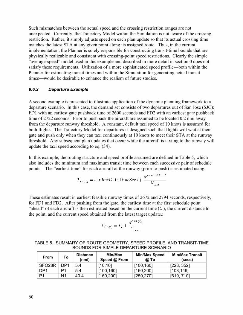
60

Such mismatches between the actual speed and the crossing restriction ranges are not unexpected. Currently, the Trajectory Model within the Simulation is not aware of the crossing restriction. Rather, it simply adjusts speed on each plan update so that its actual crossing time matches the latest STA at any given point along its assigned route. Thus, in the current implementation, the Planner is solely responsible for constructing transit-time bounds that are physically realizable and consistent with crossing-point speed restrictions. Clearly the simple “average-speed” model used in this example and described in more detail in section 0 does not satisfy these requirements. Utilization of a more sophisticated speed profile—both within the Planner for estimating transit times and within the Simulation for generating actual transit times—would be desirable to enhance the realism of future studies. 9.6.2 Departure Example

A second example is presented to illustrate application of the dynamic planning framework to a departure scenario. In this case, the demand set consists of two departures out of San Jose (SJC): FD1 with an earliest gate pushback time of 2600 seconds and FD2 with an earliest gate pushback time of 2722 seconds. Prior to pushback the aircraft are assumed to be located 0.2 nmi away from the departure runway threshold. A constant, default taxi speed of 10 knots is assumed for both flights. The Trajectory Model for departures is designed such that flights will wait at their gate and push only when they can taxi continuously at 10 knots to meet their STA at the runway threshold. Any subsequent plan updates that occur while the aircraft is taxiing to the runway will update the taxi speed according to eq. (34). In this example, the routing structure and speed profile assumed are defined in Table 5, which also includes the minimum and maximum transit time between each successive pair of schedule points. The “earliest time” for each aircraft at the runway (prior to push) is estimated using:

These estimates result in earliest feasible runway times of 2672 and 2794 seconds, respectively, for FD1 and FD2. After pushing from the gate, the earliest time at the first schedule point “ahead” of each aircraft is then estimated based on the current time ( ), the current distance to the point, and the current speed obtained from the latest target update.:

TABLE 5. SUMMARY OF ROUTE GEOMETRY, SPEED PROFILE, AND TRANSIT-TIME

BOUNDS FOR SIMPLE DEPARTURE SCENARIO

From To Distance

(nmi) Min/Max

Speed @ From Min/Max Speed

@ To Min/Max Transit

(secs)

SFO28R DP1 5.4 [10,10] [100,160] [228, 352] DP1 P1 5.4 [100,160] [160,200] [108,149] P1 N1 40.4 [160,200] [250,270] [619, 710]

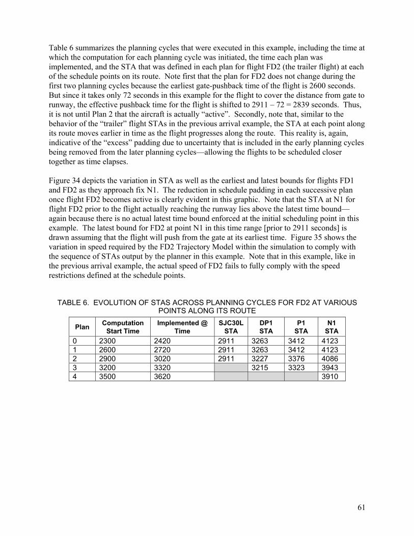
61

Table 6 summarizes the planning cycles that were executed in this example, including the time at which the computation for each planning cycle was initiated, the time each plan was implemented, and the STA that was defined in each plan for flight FD2 (the trailer flight) at each of the schedule points on its route. Note first that the plan for FD2 does not change during the first two planning cycles because the earliest gate-pushback time of the flight is 2600 seconds. But since it takes only 72 seconds in this example for the flight to cover the distance from gate to runway, the effective pushback time for the flight is shifted to 2911 – 72 = 2839 seconds. Thus, it is not until Plan 2 that the aircraft is actually “active”. Secondly, note that, similar to the behavior of the “trailer” flight STAs in the previous arrival example, the STA at each point along its route moves earlier in time as the flight progresses along the route. This reality is, again, indicative of the “excess” padding due to uncertainty that is included in the early planning cycles being removed from the later planning cycles—allowing the flights to be scheduled closer together as time elapses. Figure 34 depicts the variation in STA as well as the earliest and latest bounds for flights FD1 and FD2 as they approach fix N1. The reduction in schedule padding in each successive plan once flight FD2 becomes active is clearly evident in this graphic. Note that the STA at N1 for flight FD2 prior to the flight actually reaching the runway lies above the latest time bound—again because there is no actual latest time bound enforced at the initial scheduling point in this example. The latest bound for FD2 at point N1 in this time range [prior to 2911 seconds] is drawn assuming that the flight will push from the gate at its earliest time. Figure 35 shows the variation in speed required by the FD2 Trajectory Model within the simulation to comply with the sequence of STAs output by the planner in this example. Note that in this example, like in the previous arrival example, the actual speed of FD2 fails to fully comply with the speed restrictions defined at the schedule points.

TABLE 6. EVOLUTION OF STAS ACROSS PLANNING CYCLES FOR FD2 AT VARIOUS POINTS ALONG ITS ROUTE

Plan Computation

Start Time Implemented @

Time SJC30L

STA DP1 STA

P1 STA

N1 STA

0 2300 2420 2911 3263 3412 4123 1 2600 2720 2911 3263 3412 4123 2 2900 3020 2911 3227 3376 4086 3 3200 3320 3215 3323 3943 4 3500 3620 3910

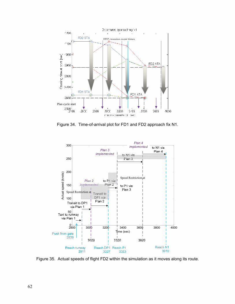
62

Figure 34. Time-of-arrival plot for FD1 and FD2 approach fix N1.

2800 3000 3200 3400 3600 3800 40000

50

100

150

200

250

300

Time (sec)

Act

ual s

peed

(kn

ots)

Figure 35. Actual speeds of flight FD2 within the simulation as it moves along its route.

FD2 crossing event times

Plan cycle start

Speed Restriction at

Speed Restriction at

63

10 SUMMARY AND LESSONS LEARNED

This chapter summarizes what we have achieved over the course of this project and the ways in which we are positioned for future work as a result.

10.1 Summary of Accomplishments Through the research conducted under this effort, we have established the feasibility of applying an optimization-based approach to the management of metroplex traffic within a real-time framework. Specifically, we have succeeded in:

• Extending previous mixed-integer-linear-program (MILP) formulations applied to network structures to allow for continuous scheduling combined with discrete route assignment and sequencing

• Developing and demonstrating a framework for dynamic planning

• Identifying and understanding issues associated with trajectory prediction and uncertainty

• Applying the MILP formulation—in both static and dynamic contexts—to metroplex interactions, demonstrating the ability for the management strategy to naturally fall out of the optimization process

• Supporting NASA Airspace Super Density Operations (SDO) researchers by providing a capability to analyze route topologies and scheduling strategies—specifically providing sequencing and route assignment search degrees of freedom (DOF) not available in their previously existing toolset

• Developing an alternate greedy first-come, first-served (FCFS) planner as a basis of comparison for evaluating the benefits of additional sequencing and route assignment options as well as proving the plug-and-play architecture that was implemented as part of this effort

• Adapting the basic MILP formulation for performance, including definition of heuristics to reduce or eliminate binary variables in some cases and utilization of alternate linearization techniques to reduce the number of auxiliary variables and constraints required to model a problem instance

Figure 36 shows a timeline view of key milestones related to the development of an optimization-based planner for metroplex operations under this NASA research announcement (NRA) effort.

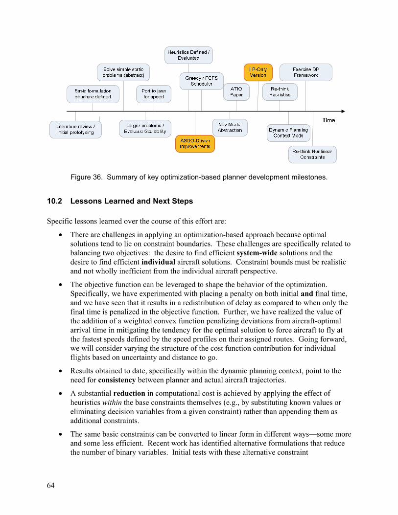
64

Figure 36. Summary of key optimization-based planner development milestones.

10.2 Lessons Learned and Next Steps Specific lessons learned over the course of this effort are:

• There are challenges in applying an optimization-based approach because optimal solutions tend to lie on constraint boundaries. These challenges are specifically related to balancing two objectives: the desire to find efficient system-wide solutions and the desire to find efficient individual aircraft solutions. Constraint bounds must be realistic and not wholly inefficient from the individual aircraft perspective.

• The objective function can be leveraged to shape the behavior of the optimization. Specifically, we have experimented with placing a penalty on both initial and final time, and we have seen that it results in a redistribution of delay as compared to when only the final time is penalized in the objective function. Further, we have realized the value of the addition of a weighted convex function penalizing deviations from aircraft-optimal arrival time in mitigating the tendency for the optimal solution to force aircraft to fly at the fastest speeds defined by the speed profiles on their assigned routes. Going forward, we will consider varying the structure of the cost function contribution for individual flights based on uncertainty and distance to go.

• Results obtained to date, specifically within the dynamic planning context, point to the need for consistency between planner and actual aircraft trajectories.

• A substantial reduction in computational cost is achieved by applying the effect of heuristics within the base constraints themselves (e.g., by substituting known values or eliminating decision variables from a given constraint) rather than appending them as additional constraints.

• The same basic constraints can be converted to linear form in different ways—some more and some less efficient. Recent work has identified alternative formulations that reduce the number of binary variables. Initial tests with these alternative constraint

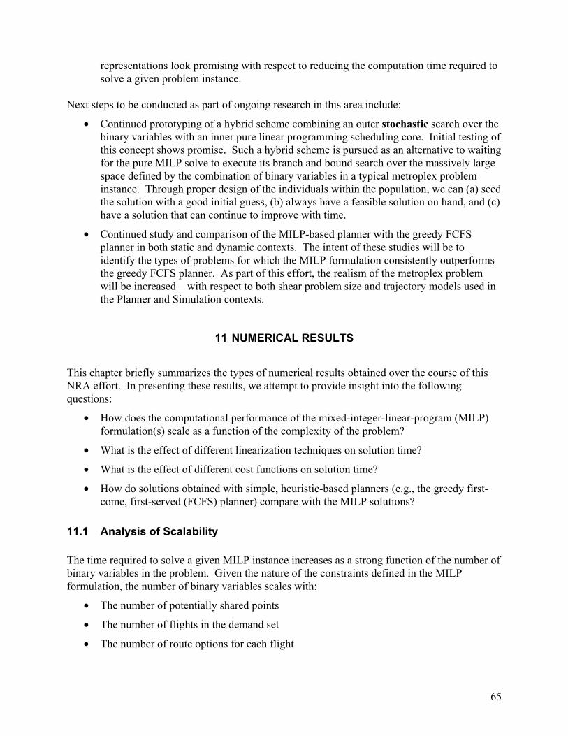
65

representations look promising with respect to reducing the computation time required to solve a given problem instance.

Next steps to be conducted as part of ongoing research in this area include:

• Continued prototyping of a hybrid scheme combining an outer stochastic search over the binary variables with an inner pure linear programming scheduling core. Initial testing of this concept shows promise. Such a hybrid scheme is pursued as an alternative to waiting for the pure MILP solve to execute its branch and bound search over the massively large space defined by the combination of binary variables in a typical metroplex problem instance. Through proper design of the individuals within the population, we can (a) seed the solution with a good initial guess, (b) always have a feasible solution on hand, and (c) have a solution that can continue to improve with time.

• Continued study and comparison of the MILP-based planner with the greedy FCFS planner in both static and dynamic contexts. The intent of these studies will be to identify the types of problems for which the MILP formulation consistently outperforms the greedy FCFS planner. As part of this effort, the realism of the metroplex problem will be increased—with respect to both shear problem size and trajectory models used in the Planner and Simulation contexts.

11 NUMERICAL RESULTS

This chapter briefly summarizes the types of numerical results obtained over the course of this NRA effort. In presenting these results, we attempt to provide insight into the following questions:

• How does the computational performance of the mixed-integer-linear-program (MILP) formulation(s) scale as a function of the complexity of the problem?

• What is the effect of different linearization techniques on solution time?

• What is the effect of different cost functions on solution time?

• How do solutions obtained with simple, heuristic-based planners (e.g., the greedy first-come, first-served (FCFS) planner) compare with the MILP solutions?

11.1 Analysis of Scalability The time required to solve a given MILP instance increases as a strong function of the number of binary variables in the problem. Given the nature of the constraints defined in the MILP formulation, the number of binary variables scales with:

• The number of potentially shared points

• The number of flights in the demand set

• The number of route options for each flight

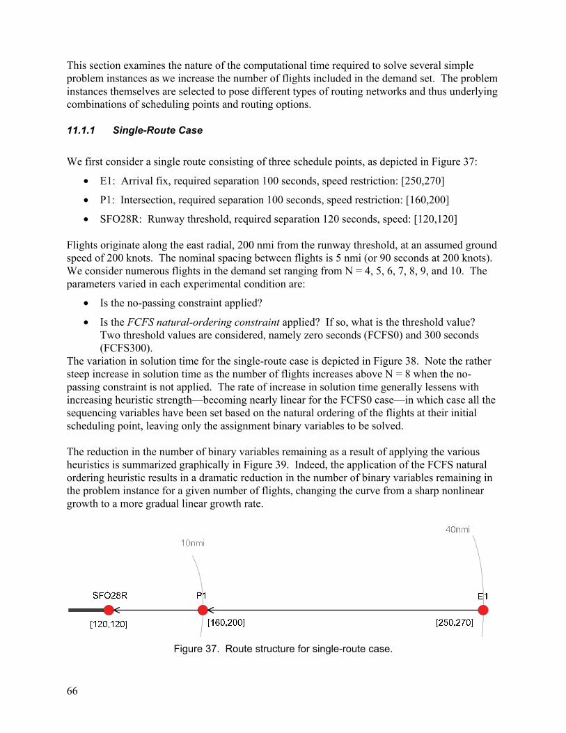
66

This section examines the nature of the computational time required to solve several simple problem instances as we increase the number of flights included in the demand set. The problem instances themselves are selected to pose different types of routing networks and thus underlying combinations of scheduling points and routing options. 11.1.1 Single-Route Case

We first consider a single route consisting of three schedule points, as depicted in Figure 37:

• E1: Arrival fix, required separation 100 seconds, speed restriction: [250,270]

• P1: Intersection, required separation 100 seconds, speed restriction: [160,200]

• SFO28R: Runway threshold, required separation 120 seconds, speed: [120,120] Flights originate along the east radial, 200 nmi from the runway threshold, at an assumed ground speed of 200 knots. The nominal spacing between flights is 5 nmi (or 90 seconds at 200 knots). We consider numerous flights in the demand set ranging from N = 4, 5, 6, 7, 8, 9, and 10. The parameters varied in each experimental condition are:

• Is the no-passing constraint applied?

• Is the FCFS natural-ordering constraint applied? If so, what is the threshold value? Two threshold values are considered, namely zero seconds (FCFS0) and 300 seconds (FCFS300).

The variation in solution time for the single-route case is depicted in Figure 38. Note the rather steep increase in solution time as the number of flights increases above N = 8 when the no-passing constraint is not applied. The rate of increase in solution time generally lessens with increasing heuristic strength—becoming nearly linear for the FCFS0 case—in which case all the sequencing variables have been set based on the natural ordering of the flights at their initial scheduling point, leaving only the assignment binary variables to be solved. The reduction in the number of binary variables remaining as a result of applying the various heuristics is summarized graphically in Figure 39. Indeed, the application of the FCFS natural ordering heuristic results in a dramatic reduction in the number of binary variables remaining in the problem instance for a given number of flights, changing the curve from a sharp nonlinear growth to a more gradual linear growth rate.

Figure 37. Route structure for single-route case.

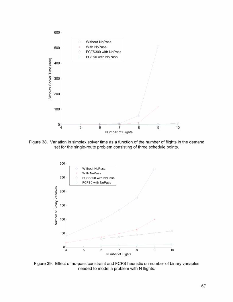
67

Figure 38. Variation in simplex solver time as a function of the number of flights in the demand set for the single-route problem consisting of three schedule points.

Figure 39. Effect of no-pass constraint and FCFS heuristic on number of binary variables needed to model a problem with N flights.

4 5 6 7 8 9 100

100

200

300

400

500

600

Number of Flights

Sim

plex

Sol

ver

Tim

e (s

ec)

Without NoPass

With NoPassFCFS300 with NoPass

FCFS0 with NoPass

4 5 6 7 8 9 100

50

100

150

200

250

300

Number of Flights

Num

ber

of B

inar

y V

aria

bles

Without NoPass

With NoPass

FCFS300 with NoPass

FCFS0 with NoPass

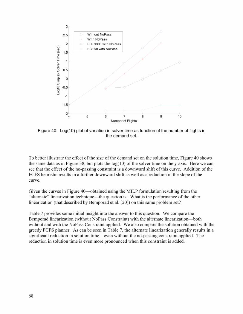
68

Figure 40. Log(10) plot of variation in solver time as function of the number of flights in the demand set.

To better illustrate the effect of the size of the demand set on the solution time, Figure 40 shows the same data as in Figure 38, but plots the log(10) of the solver time on the y-axis. Here we can see that the effect of the no-passing constraint is a downward shift of this curve. Addition of the FCFS heuristic results in a further downward shift as well as a reduction in the slope of the curve. Given the curves in Figure 40—obtained using the MILP formulation resulting from the “alternate” linearization technique—the question is: What is the performance of the other linearization (that described by Bemporad et al. [20]) on this same problem set? Table 7 provides some initial insight into the answer to this question. We compare the Bemporad linearization (without NoPass Constraint) with the alternate linearization—both without and with the NoPass Constraint applied. We also compare the solution obtained with the greedy FCFS planner. As can be seen in Table 7, the alternate linearization generally results in a significant reduction in solution time—even without the no-passing constraint applied. The reduction in solution time is even more pronounced when this constraint is added.

4 5 6 7 8 9 10-2

-1.5

-1

-0.5

0

0.5

1

1.5

2

2.5

3

Number of Flights

Log1

0 S

impl

ex S

olve

r T

ime

(sec

)

Without NoPass

With NoPass

FCFS300 with NoPass

FCFS0 with NoPass

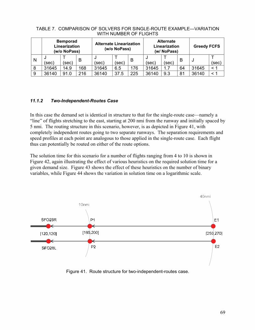
69

TABLE 7. COMPARISON OF SOLVERS FOR SINGLE-ROUTE EXAMPLE—VARIATION WITH NUMBER OF FLIGHTS

Bemporad

Linearization (w/o NoPass)

Alternate Linearization (w/o NoPass)

Alternate Linearization (w/ NoPass)

Greedy FCFS

N J (sec)

T (sec)

B J (sec)

T (sec)

B J (sec)

T (sec)

B J T (sec)

8 31645 14.9 168 31645 6.5 176 31645 1.7 64 31645 < 1 9 36140 91.0 216 36140 37.5 225 36140 9.3 81 36140 < 1

11.1.2 Two-Independent-Routes Case

In this case the demand set is identical in structure to that for the single-route case—namely a “line” of flights stretching to the east, starting at 200 nmi from the runway and initially spaced by 5 nmi. The routing structure in this scenario, however, is as depicted in Figure 41, with completely independent routes going to two separate runways. The separation requirements and speed profiles at each point are analogous to those applied in the single-route case. Each flight thus can potentially be routed on either of the route options. The solution time for this scenario for a number of flights ranging from 4 to 10 is shown in Figure 42, again illustrating the effect of various heuristics on the required solution time for a given demand size. Figure 43 shows the effect of these heuristics on the number of binary variables, while Figure 44 shows the variation in solution time on a logarithmic scale.

Figure 41. Route structure for two-independent-routes case.

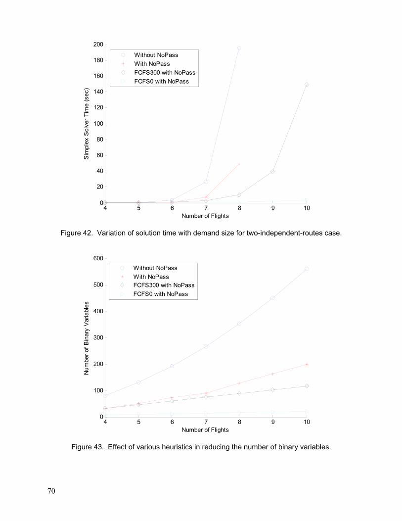
70

Figure 42. Variation of solution time with demand size for two-independent-routes case.

Figure 43. Effect of various heuristics in reducing the number of binary variables.

4 5 6 7 8 9 100

20

40

60

80

100

120

140

160

180

200

Number of Flights

Sim

plex

Sol

ver

Tim

e (s

ec)

Without NoPass

With NoPass

FCFS300 with NoPass

FCFS0 with NoPass

4 5 6 7 8 9 100

100

200

300

400

500

600

Number of Flights

Num

ber

of B

inar

y V

aria

bles

Without NoPass

With NoPassFCFS300 with NoPass

FCFS0 with NoPass

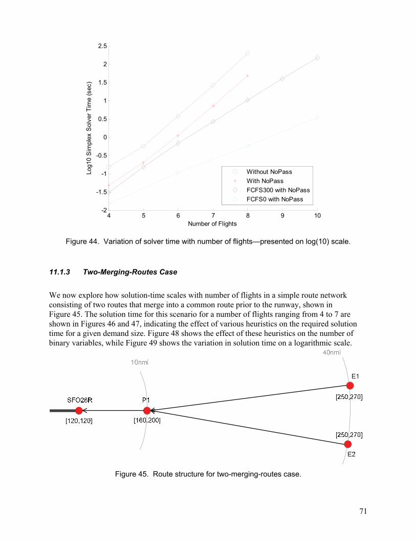
71

Figure 44. Variation of solver time with number of flights—presented on log(10) scale.

11.1.3 Two-Merging-Routes Case

We now explore how solution-time scales with number of flights in a simple route network consisting of two routes that merge into a common route prior to the runway, shown in Figure 45. The solution time for this scenario for a number of flights ranging from 4 to 7 are shown in Figures 46 and 47, indicating the effect of various heuristics on the required solution time for a given demand size. Figure 48 shows the effect of these heuristics on the number of binary variables, while Figure 49 shows the variation in solution time on a logarithmic scale.

Figure 45. Route structure for two-merging-routes case.

4 5 6 7 8 9 10-2

-1.5

-1

-0.5

0

0.5

1

1.5

2

2.5

Number of Flights

Log1

0 S

impl

ex S

olve

r T

ime

(sec

)

Without NoPass

With NoPass

FCFS300 with NoPass

FCFS0 with NoPass

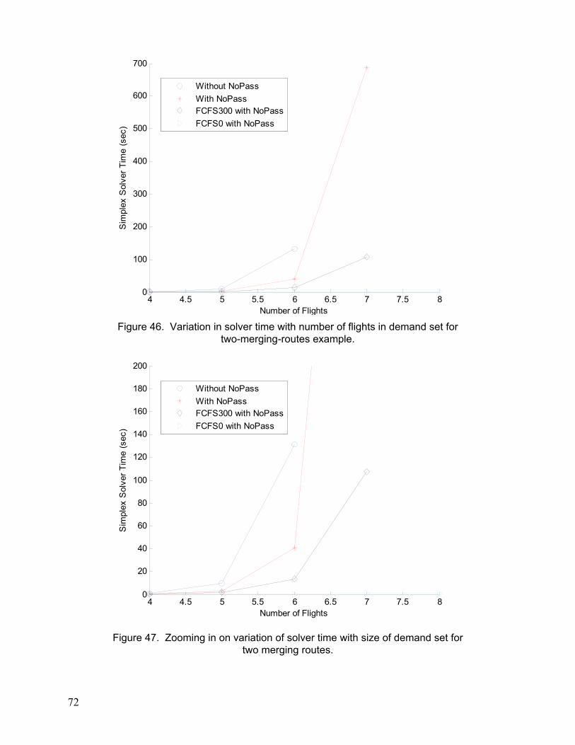
72

Figure 46. Variation in solver time with number of flights in demand set for two-merging-routes example.

Figure 47. Zooming in on variation of solver time with size of demand set for two merging routes.

4 4.5 5 5.5 6 6.5 7 7.5 80

100

200

300

400

500

600

700

Number of Flights

Sim

plex

Sol

ver

Tim

e (s

ec)

Without NoPass

With NoPassFCFS300 with NoPass

FCFS0 with NoPass

4 4.5 5 5.5 6 6.5 7 7.5 80

20

40

60

80

100

120

140

160

180

200

Number of Flights

Sim

plex

Sol

ver

Tim

e (s

ec)

Without NoPass

With NoPassFCFS300 with NoPass

FCFS0 with NoPass

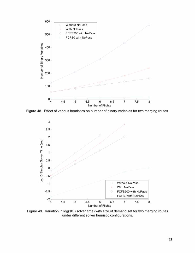
73

Figure 48. Effect of various heuristics on number of binary variables for two merging routes.

Figure 49. Variation in log(10) (solver time) with size of demand set for two merging routes under different solver heuristic configurations.

4 4.5 5 5.5 6 6.5 7 7.5 80

100

200

300

400

500

600

Number of Flights

Num

ber

of B

inar

y V

aria

bles

Without NoPass

With NoPassFCFS300 with NoPass

FCFS0 with NoPass

4 4.5 5 5.5 6 6.5 7 7.5 8-2

-1.5

-1

-0.5

0

0.5

1

1.5

2

2.5

3

Number of Flights

Log1

0 S

impl

ex S

olve

r T

ime

(sec

)

Without NoPass

With NoPass

FCFS300 with NoPass

FCFS0 with NoPass

74

11.1.4 Effect of Penalty on Initial Time

We also briefly explored the effect of adding a penalty on initial time to the objective function. It results in an objective function of the form:

Single-Route Case

For the single-route case, Table8 illustrates the impact of adding the cost component related to the time at the initial scheduling point. Note that the objective function value—as defined as the sum of only the times at the final scheduling point—remains unchanged using either cost function. However, there is an impact on the solution time required; the time required to obtain the solution was reduced by approximately 40% for the N = 10 flight case. In addition, although the total delay is the same for both cost functions, the distribution of delay in the two cases is different. For the case where the time at the initial scheduling point is included in the cost function, the delay tends to be incurred within the route (e.g., via speed reduction), whereas with the original cost function the delay is incurred prior to the initial scheduling point.

Two-Independent-Routes Case

A similar trend to that observed previously in the single-route case is observed in Table 9 for the two-independent-routes case. However, the impact of adding the penalty on time at the initial scheduling point is not quite as dramatic in this scenario, but still reduces the solution time required by approximately 30% for the N = 9 flights case.

TABLE 8. EFFECT OF ADDING INITIAL TIME PENALTY ON SOLUTION TIME AND

SOLUTION OBTAINED FOR SINGLE-ROUTE CASE

Final Time Penalty Initial and Final Time Penalty

Num Flights

Soln Time (sec)

(sec)

Total Delay (sec)

Soln Time (sec) (sec)

Total Delay (sec)

8 1.7 31645 1215 1.0 31645 1215 9 9.344 36140 1562 5.75 36140 1562 10 58.875 40756 1953 35.875 40756 1953

TABLE 9. EFFECT OF ADDING PENALTY ON TIME AT INITIAL SCHEDULING POINT ON SOLUTION TIME FOR TWO INDEPENDENT ROUTES

Final Time Penalty Initial and Final Time Penalty

Num Flights

Soln Time (sec)

(sec)

Total Delay (sec)

Soln Time (sec) (sec)

Total Delay (sec)

6 0.422 22962 0 0.375 22962 0 7 1.765 27047 0 1.453 27047 0 8 8.157 31225 0 6.125 31225 0 9 37.563 35463 0 25.984 35463 0

75

TABLE 10. EFFECT OF PENALTY ON TIME AT INITIAL SCHEDULING POINT ON SOLUTION TIME FOR THE TWO-MERGING-ROUTES CASE

Final Time Penalty Initial and Final Time Penalty

Num Flights

Soln Time (sec)

(sec)

Total Delay (sec)

Soln Time (sec) (sec)

Total Delay (sec)

5 1.109 19514 439 0.765 19514 439 6 11.625 23777 659 8.016 23777 659 7 106.9 28160 922 75.0 28160 922

Two-Merging-Routes Case

As a final example, we compare the solution times required for the two-merging-routes case when a penalty on time at the initial point is added to the cost function. As summarized in Table 10, again the effect of adding this penalty is to reduce the solution time (by ~30% for the N = 7 case) with an identical solution from the perspective of “final time” and total delay.

11.2 Comparison against Greedy FCFS Planner This section compares the computational time required to solve a given problem instance with the MILP planner (alternate linearization) with that required by the greedy FCFS planner. We also compare the nature of the solutions obtained in terms of the equivalent objective function value obtained, and the nature of the delays found in the solution. The time required for the greedy FCFS planner to solve problems involving hundreds of flights is inconsequential—on the order of less than 1 second of CPU time. Thus, from a pure speed- of-performance perspective, the greedy FCFS planner significantly outperforms the MILP implementation using lpsolve. So the question really becomes: Under what conditions does the MILP solution provide a “better” answer? And what is “better”? It should be noted that the greedy FCFS planner objective function implemented in the initial set of comparisons presented in this section is to select the minimum delay route. This planner is slightly different from the MILP planner, which tries to minimize the total exit time out of the metroplex over all flights in the demand set. 11.2.1 Single-Route Case with Alternating Aircraft Types

We first investigate a case in which the MILP planner should outperform the greedy FCFS planner from a runway-throughput perspective. We consider a set of eight departures from a single airport on a single runway. All aircraft originate at same location (200,0). Four of the aircraft are “heavies” and four of the aircraft are “smalls”. The earliest gate-pushback time for this set of flights is defined such that their natural FCFS ordering at the runway is H, S, H, S, H, S, H, S. The separation matrix used at the runway in this scenario requires 180 seconds for an “S” following an “H” and 90 seconds otherwise. In other words, the natural ordering corresponds to an inefficient use of the runway as the required gaps are larger than if the flights were grouped according to size. Uncertainty in arrival time is assumed to be zero at all points (no buffering).

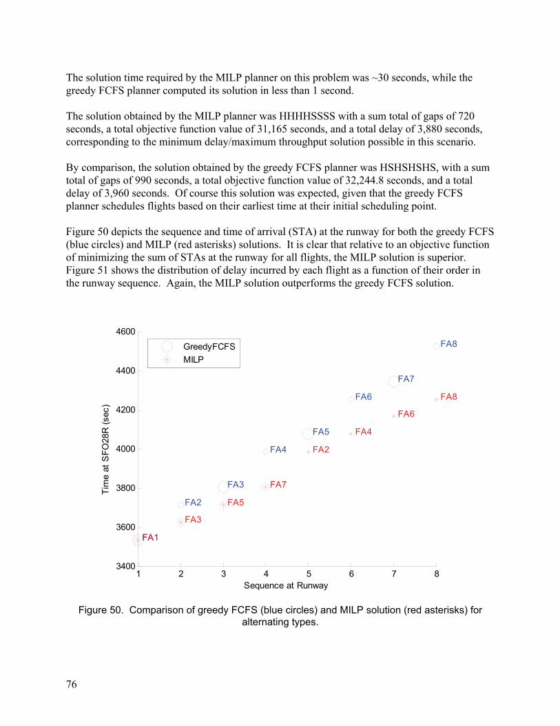
76

The solution time required by the MILP planner on this problem was ~30 seconds, while the greedy FCFS planner computed its solution in less than 1 second. The solution obtained by the MILP planner was HHHHSSSS with a sum total of gaps of 720 seconds, a total objective function value of 31,165 seconds, and a total delay of 3,880 seconds, corresponding to the minimum delay/maximum throughput solution possible in this scenario. By comparison, the solution obtained by the greedy FCFS planner was HSHSHSHS, with a sum total of gaps of 990 seconds, a total objective function value of 32,244.8 seconds, and a total delay of 3,960 seconds. Of course this solution was expected, given that the greedy FCFS planner schedules flights based on their earliest time at their initial scheduling point. Figure 50 depicts the sequence and time of arrival (STA) at the runway for both the greedy FCFS (blue circles) and MILP (red asterisks) solutions. It is clear that relative to an objective function of minimizing the sum of STAs at the runway for all flights, the MILP solution is superior. Figure 51 shows the distribution of delay incurred by each flight as a function of their order in the runway sequence. Again, the MILP solution outperforms the greedy FCFS solution.

Figure 50. Comparison of greedy FCFS (blue circles) and MILP solution (red asterisks) for alternating types.

1 2 3 4 5 6 7 83400

3600

3800

4000

4200

4400

4600

FA1FA1

Sequence at Runway

Tim

e at

SF

O28

R (

sec)

FA2

FA3

FA3

FA5

FA4

FA7

FA5

FA2

FA6

FA4

FA7

FA6

FA8

FA8

GreedyFCFS

MILP

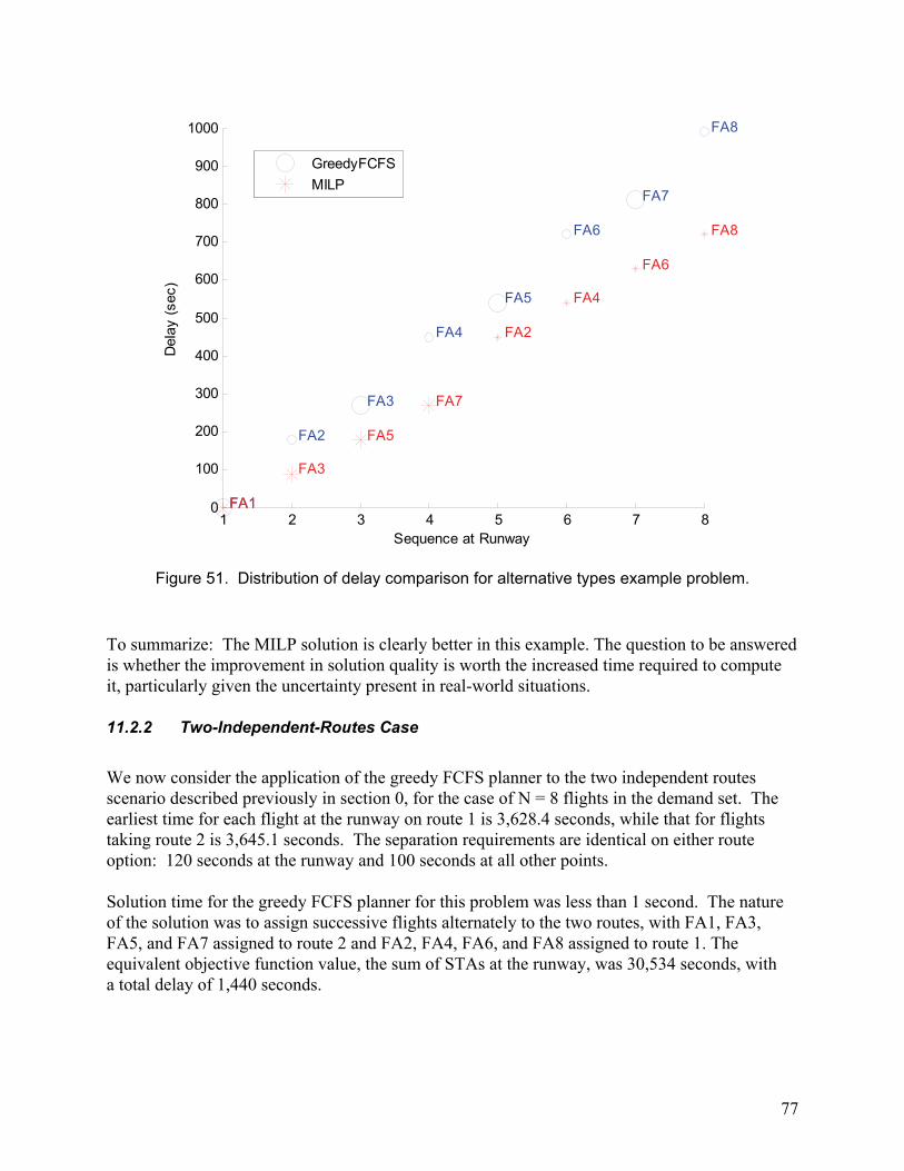
77

Figure 51. Distribution of delay comparison for alternative types example problem.

To summarize: The MILP solution is clearly better in this example. The question to be answered is whether the improvement in solution quality is worth the increased time required to compute it, particularly given the uncertainty present in real-world situations. 11.2.2 Two-Independent-Routes Case

We now consider the application of the greedy FCFS planner to the two independent routes scenario described previously in section 0, for the case of N = 8 flights in the demand set. The earliest time for each flight at the runway on route 1 is 3,628.4 seconds, while that for flights taking route 2 is 3,645.1 seconds. The separation requirements are identical on either route option: 120 seconds at the runway and 100 seconds at all other points. Solution time for the greedy FCFS planner for this problem was less than 1 second. The nature of the solution was to assign successive flights alternately to the two routes, with FA1, FA3, FA5, and FA7 assigned to route 2 and FA2, FA4, FA6, and FA8 assigned to route 1. The equivalent objective function value, the sum of STAs at the runway, was 30,534 seconds, with a total delay of 1,440 seconds.

1 2 3 4 5 6 7 80

100

200

300

400

500

600

700

800

900

1000

FA1FA1

Sequence at Runway

Del

ay (

sec)

FA2

FA3

FA3

FA5

FA4

FA7

FA5

FA2

FA6

FA4

FA7

FA6

FA8

FA8

GreedyFCFS

MILP

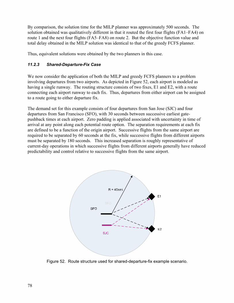
78

By comparison, the solution time for the MILP planner was approximately 500 seconds. The solution obtained was qualitatively different in that it routed the first four flights (FA1–FA4) on route 1 and the next four flights (FA5–FA8) on route 2. But the objective function value and total delay obtained in the MILP solution was identical to that of the greedy FCFS planner. Thus, equivalent solutions were obtained by the two planners in this case. 11.2.3 Shared-Departure-Fix Case

We now consider the application of both the MILP and greedy FCFS planners to a problem involving departures from two airports. As depicted in Figure 52, each airport is modeled as having a single runway. The routing structure consists of two fixes, E1 and E2, with a route connecting each airport runway to each fix. Thus, departures from either airport can be assigned to a route going to either departure fix. The demand set for this example consists of four departures from San Jose (SJC) and four departures from San Francisco (SFO), with 30 seconds between successive earliest gate-pushback times at each airport. Zero padding is applied associated with uncertainty in time of arrival at any point along each potential route option. The separation requirements at each fix are defined to be a function of the origin airport. Successive flights from the same airport are required to be separated by 60 seconds at the fix, while successive flights from different airports must be separated by 180 seconds. This increased separation is roughly representative of current-day operations in which successive flights from different airports generally have reduced predictability and control relative to successive flights from the same airport.

Figure 52. Route structure used for shared-departure-fix example scenario.

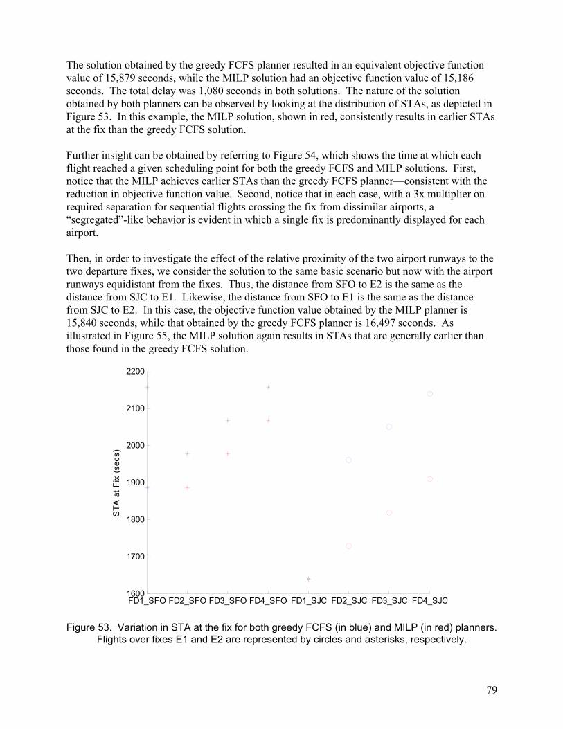
79

The solution obtained by the greedy FCFS planner resulted in an equivalent objective function value of 15,879 seconds, while the MILP solution had an objective function value of 15,186 seconds. The total delay was 1,080 seconds in both solutions. The nature of the solution obtained by both planners can be observed by looking at the distribution of STAs, as depicted in Figure 53. In this example, the MILP solution, shown in red, consistently results in earlier STAs at the fix than the greedy FCFS solution. Further insight can be obtained by referring to Figure 54, which shows the time at which each flight reached a given scheduling point for both the greedy FCFS and MILP solutions. First, notice that the MILP achieves earlier STAs than the greedy FCFS planner—consistent with the reduction in objective function value. Second, notice that in each case, with a 3x multiplier on required separation for sequential flights crossing the fix from dissimilar airports, a “segregated”-like behavior is evident in which a single fix is predominantly displayed for each airport. Then, in order to investigate the effect of the relative proximity of the two airport runways to the two departure fixes, we consider the solution to the same basic scenario but now with the airport runways equidistant from the fixes. Thus, the distance from SFO to E2 is the same as the distance from SJC to E1. Likewise, the distance from SFO to E1 is the same as the distance from SJC to E2. In this case, the objective function value obtained by the MILP planner is 15,840 seconds, while that obtained by the greedy FCFS planner is 16,497 seconds. As illustrated in Figure 55, the MILP solution again results in STAs that are generally earlier than those found in the greedy FCFS solution.

Figure 53. Variation in STA at the fix for both greedy FCFS (in blue) and MILP (in red) planners. Flights over fixes E1 and E2 are represented by circles and asterisks, respectively.

FD1_SFO FD2_SFO FD3_SFO FD4_SFO FD1_SJC FD2_SJC FD3_SJC FD4_SJC1600

1700

1800

1900

2000

2100

2200

ST

A a

t F

ix (

secs

)

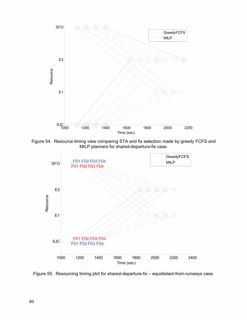
80

Figure 54. Resource timing view comparing STA and fix selection made by greedy FCFS and MILP planners for shared-departure-fix case.

Figure 55. Resourcing timing plot for shared-departure-fix – equidistant-from-runways case.

1000 1200 1400 1600 1800 2000 2200SJC

E1

E2

SFO

Time (sec)

Res

ourc

e

GreedyFCFS

MILP

1000 1200 1400 1600 1800 2000 2200 2400

SJC

E1

E2

SFO

Time (sec)

Res

ourc

e

FD1 FD2 FD3 FD4

FD1 FD2 FD3 FD4

FD1 FD2 FD3 FD4

FD1 FD2 FD3 FD4

GreedyFCFS

MILP

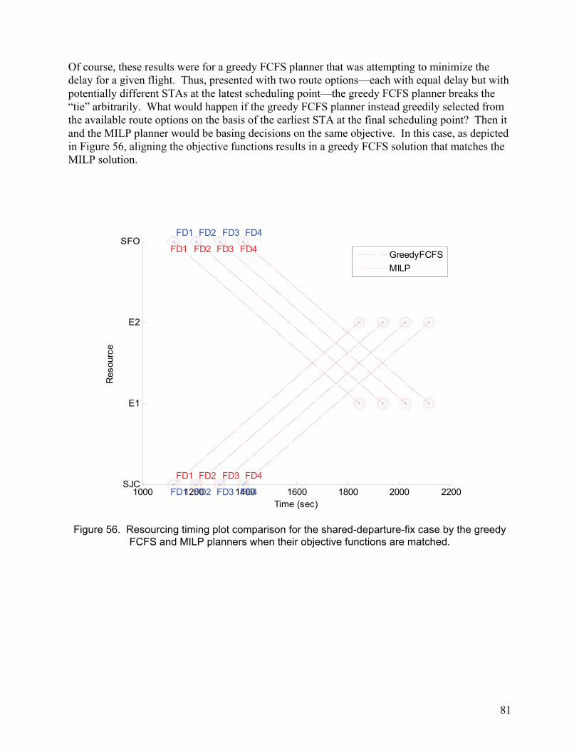
81

Of course, these results were for a greedy FCFS planner that was attempting to minimize the delay for a given flight. Thus, presented with two route options—each with equal delay but with potentially different STAs at the latest scheduling point—the greedy FCFS planner breaks the “tie” arbitrarily. What would happen if the greedy FCFS planner instead greedily selected from the available route options on the basis of the earliest STA at the final scheduling point? Then it and the MILP planner would be basing decisions on the same objective. In this case, as depicted in Figure 56, aligning the objective functions results in a greedy FCFS solution that matches the MILP solution.

Figure 56. Resourcing timing plot comparison for the shared-departure-fix case by the greedy FCFS and MILP planners when their objective functions are matched.

1000 1200 1400 1600 1800 2000 2200SJC

E1

E2

SFO

Time (sec)

Res

ourc

e

FD1 FD2 FD3 FD4

FD1 FD2 FD3 FD4

FD1 FD2 FD3 FD4

FD1 FD2 FD3 FD4

GreedyFCFS

MILP

82

12 DYNAMIC PLANNING DEPLOYMENT

This section presents information on running the dynamic metroplex planning software.

12.1 System Requirements and Configuration

• Java Runtime Environment: Install either Java Runtime Environment (JRE) version 6.0 or higher. Be sure that JRE bin directory is in the system path.

• MATLAB: Version 7.9.0 was used in testing of this software.

• LPSolve : This linear programming library is required to run the suggested planner implementation (i.e., the Mixed Planner). Library files applicable to the operating system must be placed in the metroplex root directory (e.g., C:/metroplex/).

o On UNIX or Linux: Copy the .a and .so library files appropriate to the bit type of the operating system to the metroplex directory (see sub-bullet).

32-bit original library files: Copy liblpsolve55.32bit.a, liblpsolve55.32bit.so, and liblpsolve55j.32bit.so to liblpsolve55.a, liblpsolve55.so, and liblpsolve55j.so appropriately.

64-bit original library files: Copy liblpsolve55.32bit.a, liblpsolve55.32bit.so, and liblpsolve55j.32bit.so to liblpsolve55.a, liblpsolve55.so, and liblpsolve55j.so appropriately.

o On Windows: Copy appropriate operating system bit type .dll files to lpsolve55.dll and lpsolve55j.dll in the metroplex directory.

12.2 Application Configuration Configuration options are available to the dynamic planning application via an application context file (see <metroplex>/config/app/dynPlanAppContext.xml). The application context consists of various application components that are specified as Java beans using Extensible Markup Language (XML). These planning application components are described in this section. 12.2.1 Planning Controller

The planning controller references and controls access to all of the components within the application context. 12.2.2 Plan Constraint Manager

The plan constraint manager holds various constraints to be considered by the Planner. Table 11 describes the constraints.

83

TABLE 11. CONSTRAINTS CONSIDERED BY THE PLANNER

Constraint Property Name Description Values

useEarliestTimeFcfs Use the earliest physically feasible time of the flights (regardless of their position) to determine first-come, first-served (FCFS) ordering. Set property minThresholdSecondsFcfs to desired threshold value. Note: Only one use*Fcfs property may be set to true for a given planning session.

true | false

userFirstCommonPointFcfs Use the unimpeded times at the first common point shared by flights as the basis for FCFS ordering. Set property minThresholdSecondsFcfs to desired threshold value. Note: Only one use*Fcfs property may be set to true for a given planning session.

true | false

useLastCommonPointFcfs Use the unimpeded times at the last common point shared by flights as the basis for FCFS ordering. Set property minThresholdSecondsFcfs to desired threshold value. Note: Only one use*Fcfs property may be set to true for a given planning session.

true | false

minThresholdSecondsFcfs In order for flights to be considered for FCFS ordering, the difference between their times being compared must be greater than this threshold. For example, if useFirstCommonPointFcfs is true, the difference between the unimpeded times at the first common point for two flights must be greater than the minThreasholdSecondsFcfs value.

[0, 1, 2, … n]

doWindowing Break down demand into a sequential set of smaller demand "windows". Set property windowSeconds for the time size of each “window”.

true | false

windowSeconds Size of each time “window” in seconds. Property doWindowing must be true for this to be applicable.

[0, 1, 2, … n]

timeoutSeconds Time at which the lpsolver will terminate and provide its current solution. If set to zero, no timeout will be applied.

[0, 1, 2, … n]

earliestTimeDeviationWeight Penalty for deviating the schedule of a flight from its aircraft optimal schedule.

Double precision integer

useFCFSBailIfSwap If a swap in the natural order of flights being compared occurs, do not apply FCFS constraint on that flight pair.

true | false

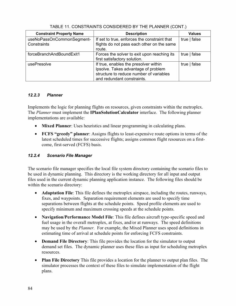
84

TABLE 11. CONSTRAINTS CONSIDERED BY THE PLANNER (CONT.)

Constraint Property Name Description Values

useNoPassOnCommonSegment-Constraints

If set to true, enforces the constraint that flights do not pass each other on the same route.

true | false

forceBranchAndBoundExit1 Forces the solver to exit upon reaching its first satisfactory solution.

true | false

usePresolve If true, enables the presolver within lpsolve. Takes advantage of problem structure to reduce number of variables and redundant constraints.

true | false

12.2.3 Planner

Implements the logic for planning flights on resources, given constraints within the metroplex. The Planner must implement the IPlanSolutionCalculator interface. The following planner implementations are available:

• Mixed Planner: Uses heuristics and linear programming in calculating plans.

• FCFS “greedy” planner: Assigns flights to least-expensive route options in terms of the latest scheduled times for successive flights; assigns common flight resources on a first-come, first-served (FCFS) basis.

12.2.4 Scenario File Manager

The scenario file manager specifies the local file system directory containing the scenario files to be used in dynamic planning. This directory is the working directory for all input and output files used in the current dynamic planning application instance. The following files should be within the scenario directory:

• Adaptation File: This file defines the metroplex airspace, including the routes, runways, fixes, and waypoints. Separation requirement elements are used to specify time separations between flights at the schedule points. Speed profile elements are used to specify minimum and maximum crossing speeds at the schedule points.

• Navigation/Performance Model File: This file defines aircraft type-specific speed and fuel usage in the overall metroplex, at fixes, and/or at runways. The speed definitions may be used by the Planner. For example, the Mixed Planner uses speed definitions in estimating time of arrival at schedule points for enforcing FCFS constraints.

• Demand File Directory: This file provides the location for the simulator to output demand set files. The dynamic planner uses these files as input for scheduling metroplex resources.

• Plan File Directory This file provides a location for the planner to output plan files. The simulator processes the context of these files to simulate implementation of the flight plans.

85

12.2.5 Dynamic Plan Manager

The Dynamic Plan Manager manages parameters specific to dynamic planning. The parameters include the following:

• Solution coverage seconds: Time horizon covered by a plan.

• Plan computation time seconds: Time estimated for the planner to compute a plan on a demand set.

• Iteration interval seconds: Frequency at which the planner is to be invoked.

• Raw demand file: The “target report” input to the simulator; it specifies the time at which each “target” appears, trajectory information, and basic flight plans.

• Latest demand set reference file: Holds reference to the latest demand set.

• Latest plan reference file: Holds reference to the latest plan.

• Freeze strategy: Refers to the application context freeze strategy.

• Apply freeze horizon: Specifies whether to apply the freeze strategy in planning.

• Freeze horizon: Specifies the freeze horizon to be used by the freeze strategy. 12.2.6 Demand Manager

Loads the demand sets from the specified data source. Currently the demand manager implementation loads the demand sets from a file. Note: Future demand managers may load demand sets programmatically. 12.2.7 Navigation Performance Manager

The navigation performance manager loads the navigation/performance model file to instantiate navigation/performance models. 12.2.8 Uncertainty Calculator

The uncertainty calculator computes expected uncertainty of the time of arrival of the flights at schedule points along prospective routes. Uncertainty calculators must implement the IUncertaintyCalculator interface. Uncertainty calculator implementations available are the following:

• UncertaintyCalculator: Applies scaled uncertainty buffer times to flights based on their distance to respective scheduled points.

• UncertaintyCalculatorUnScaled: Applies rigid unscaled uncertainty buffer times to flights based on their distance to respective scheduled points

86

12.2.9 Freeze Strategy

The freeze strategy implements the way in which metroplex resources are to be locked onto flights. All freeze strategies must implement the IFreezeStrategy interface. The freeze strategy currently available follows:

• FreezeAllAtFirstPointStrategy: Freezes the currently scheduled times at all schedule points for the assigned route upon the flight coming within the freeze horizon time of the first schedule point on the currently assigned route of the flight.

12.3 Running the Dynamic Planning Application The dynamic planning application requires startup of the dynamic planning and simulation components. As depicted in the section “Dynamic Planning Applications”, theplanner and simulator have “listeners” for the latest demand set and plan files, respectively. This section describes the steps required to run the dynamic planning application and verify results. 12.3.1 Planner Startup

The dynamic planner requires that a process be started that “listens” for changes to the latest demand set reference file (i.e., <scenario directory>/ LatestDemandSet.xml). Execute the following within a command prompt window:

• cd bin

• dynPlanner.bat or dynPlanner.sh The command window standard output should show something to the effect that the planner is waiting for changes to the latest demand set file, such as:

• Waiting for new demand set changes in <scenario directory>/LatestDemandSet.xml When the planner receives demand sets from the simulator, it in turn produces plans and writes them out to <scenario directory>/LatestPlan.xml. The planner shuts down upon producing the number of plans equal to the maxPlans property value as specified in the application context bean element DynamicPlanManager. Otherwise the user should kill the process (e.g., Ctrl-C).

87

12.3.2 Simulator Startup

The simulator requires “target report” information. A raw demand file (as specified in the application context file) is used to provide this information as input to the simulator. The simulator must be launched from MATLAB. The following steps describe how to launch the simulator:

1. Start MATLAB.

2. Set the MATLAB Current Folder to metroplex root directory.

3. Show the Current Folder panel on the MATLAB Desktop by selecting Desktop – Current Folder.

4. Within the Current Folder panel, navigate to <metroplex>/Optimization/Simulation/ MatLab/.

5. Select file DynamicPlanningSimMain.m, right mouse click it, and select Run File. The simulator reads in the raw demand set file, produces a demand set file to <scenario directory>/DemandFiles/, and updates the latest demand set reference file. Then a message stating that the simulator is waiting while the plan iteration completes should show to the MATLAB command window: Waiting for plan for iteration 0 to complete The simulator shuts down if an update to the latest plan reference file is not detected within the default timeout time of 120 seconds.

12.4 Dynamic Planning Verification When the simulator completes implementation of a plan, it produces a demand set file and writes it to <scenario directory>/DemandFiles/. Likewise, the planner produces plans and writes them to <scenario directory>/PlanFiles/. Until either the simulator or planner is shut down, demand set files and plan files are written to the appropriate sub-directories under the scenario directory. In addition, the simulated flight information is available in MATLAB workspace objects for verification. This section describes how to verify dynamic planning via these outputs. 12.4.1 Demand Set File Verification

When the time stamp of a flight “target” (as found in the scenario raw demand file) is found within the planning horizon, an entry for that flight is written to the demand set file produced by the simulator. The X/Y coordinates of a flight previously “scheduled” by the planner should approach the next schedule point of the route currently assigned to the flight. The speed of a flight should ideally fall within the maximum and minimum required speeds of the next schedule point and previous schedule point (if any).

88

Demand Set File Contents

Demand set files produced by the simulator contain the following data:

• Elapsed seconds: The time that has elapsed since the start of the startup of dynamic planning. This parameter may commonly be referred to as the “plan time”.

• Flights: Data for each flight.

o ID: Flight ID.

o Type: Aircraft type corresponding to the “type” attributes of the elements specified in the Navigation/Performance scenario file.

o Category: “A” for arrival to a metroplex airport or “D” for departure from a metroplex airport.

o Origin airport: Origin airport code (significant for metroplex departures).

o Destination airport: Destination airport code (significant for metroplex arrivals).

o Direction: Directions are with respect to the “center” of the metroplex. (Important: For a flight to be scheduled on a metroplex route, the direction value must correspond with the direction attribute value for one or more fixes as defined in the scenario adaptation XML file).

For arrival flight: Direction from which a flight is entering the metroplex at its arrival fix.

For departure flight: Direction to where a flight is exiting the metroplex at its departure fix.

o Current X nmi: X coordinate in nautical miles with respect to the “center” of the metroplex.

o Current Y nmi: Y coordinate in nautical miles with respect to the “center” of the metroplex.

o Current altitude feet: Altitude in feet.

o Current heading degrees: Heading in degrees with respect to the “center” of the metroplex.

o Current speed knots: Ground speed in knots.

o Route (optional): Assigned route for the flight.

o Fix (optional): Assigned fix for a flight. 12.4.2 Plan File Verification

As a demand set is processed by the planner, each flight is assigned a route. For each schedule point ahead of the flight along the route, crossing times are estimated based on resource constraints and aircraft performance limitations. If a freeze strategy is configured for the dynamic planning session, a flight found within the freeze horizon of an applicable schedule point will have its route assignment frozen and possibly its scheduled times of arrival (STAs) on one or more schedule points remaining along the assigned route.

89

Plan File Contents

Plan files produced by the planner consist of the following data:

• Elapsed seconds: The time that has elapsed since the start of the startup of dynamic planning. This may commonly be referred to as the “plan time”.

• Flights: Data for each flight.

o ID: Flight ID.

o Route: Currently assigned route.

o Route assignment frozen: Boolean flag indicating whether the route assignment is “frozen”.

o Schedule points: Fix, waypoint(s), and runway found ahead of the flight on the currently assigned route.

Reference ID: Schedule point identifier corresponding to the ID used for the schedule point in the scenario adaptation file.

Scheduled crossing time seconds (STA): Crossing time as scheduled by the planner.

Schedule cross time frozen: Boolean indicator as to whether the scheduled crossing time is frozen.

Earliest time seconds: Earliest time physically feasible for the flight to cross the scheduled point.

Latest time seconds: Latest time for the flight to physically cross the scheduled point.

Unimpeded crossing time seconds: The aircraft-optimal time at which the flight would cross the schedule point if allowed to fly completely uninfluenced by the presence of any other flights.

12.4.3 Verification in MATLAB

The simulator in MATLAB provides a means for animating the implementation of the flights based on their schedules. Plots may be generated based on MATLAB data objects resulting from the dynamic planning simulation.

Simulation Animation

Upon simulator startup, a MATLAB figure window displays the metroplex adaptation and the active flight “targets”. As the simulator detects and implements newly received plans, the flights advance to their next schedule points to meet the currently scheduled STAs. Flights should advance along their assigned or frozen routes. Flights should maintain required separation at schedule points both in cases of leader/follower instances along the same route and in cases where assigned routes intersect.

90

Figure 57 shows an animation of arrival flight FA1 approaching runway SFO28R and departure flight FD1 approaching schedule point DP1 after departing from runway SJC30L. The adaptation demonstrates the use of routes intersecting at a common schedule point P1.

Plot Verification

Upon completion of a dynamic planning and simulation session, plots may be generated on the resulting MATLAB data objects. Plots such as the ones in Figure 58 may be used to compare various times of arrival. These plots were generated using script <metroplex>/Optimization/ Simulation/MatLab/createTimeOfArrivalGraphic.m. For the purposes of showing more clearly the various times of arrival, Figure 59 is a close-up figure focusing only on arrival flights FA1 and FA2.

Figure 57. Depiction of flight FA1 approaching runway SFO28R and flight FD1 approaching schedule point DP1.

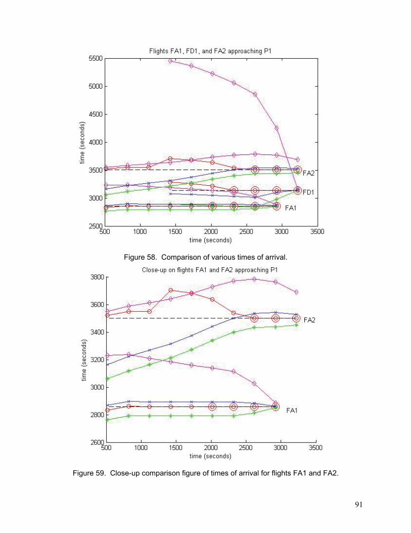
91

Figure 58. Comparison of various times of arrival.

Figure 59. Close-up comparison figure of times of arrival for flights FA1 and FA2.

92

The lines are explained as follows:

• Dashed line: Actual time of arrival (ATA) at schedule point.

• Red circles (small) and red lines: Scheduled time of arrival (STA) at schedule point.

• Red circles (large): Frozen STAs on schedule point.

• Blue X symbols and lines: Aircraft-optimal time of arrival at schedule point.

• Green asterisk symbols and lines: Earliest physically feasible time of arrival at schedule point.

• Magenta diamonds and lines: Latest physically feasible time of arrival at schedule point.

A few things worth noting regarding these two plots follow:

• As the flights approach the schedule point, their STAs converge on the ATAs.

• STAs do not change once frozen for a flight on the schedule point. (See the large red circles in the figures.)

• STAs may be found outside of the estimated earliest or latest times of arrival if the aircraft is still “outside” of the metroplex. For example, at 1300 seconds the STA for FA2 exceeds the estimated latest time of arrival. This “spike” in the STA for FA2 is due to the planner scheduling departure flight FD1 ahead of FA2 at common schedule point P1. This STA value is reasonable since FA2 is over 180 nmi from the radial boundary of metroplex.

• Earliest and latest times of arrival typically approach but often do not intersect with the ATA.

• The time gap between the earliest and latest times of arrival for a flight will decrease as the flight approaches its ATA.

To produce the time-of-arrival plot, execute the script in the following manner:

• createTimeOfArrivalGraphic(2,flights, 'P1') Parameter description:

• 2: Arbitrary number for the MATLAB figure.

• flights: Data collection of flight objects that hold the time-of-arrival data.

• ‘P1’: Name of the schedule point of interest.

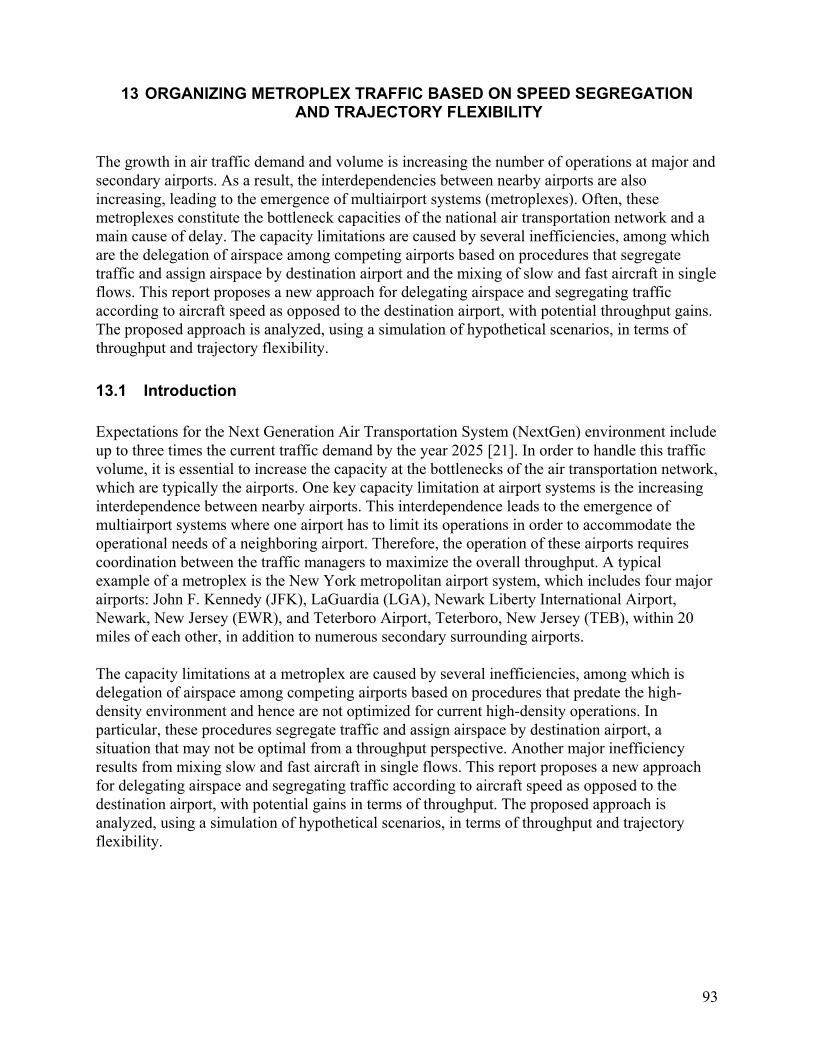
93

13 ORGANIZING METROPLEX TRAFFIC BASED ON SPEED SEGREGATION AND TRAJECTORY FLEXIBILITY

The growth in air traffic demand and volume is increasing the number of operations at major and secondary airports. As a result, the interdependencies between nearby airports are also increasing, leading to the emergence of multiairport systems (metroplexes). Often, these metroplexes constitute the bottleneck capacities of the national air transportation network and a main cause of delay. The capacity limitations are caused by several inefficiencies, among which are the delegation of airspace among competing airports based on procedures that segregate traffic and assign airspace by destination airport and the mixing of slow and fast aircraft in single flows. This report proposes a new approach for delegating airspace and segregating traffic according to aircraft speed as opposed to the destination airport, with potential throughput gains. The proposed approach is analyzed, using a simulation of hypothetical scenarios, in terms of throughput and trajectory flexibility.

13.1 Introduction Expectations for the Next Generation Air Transportation System (NextGen) environment include up to three times the current traffic demand by the year 2025 [21]. In order to handle this traffic volume, it is essential to increase the capacity at the bottlenecks of the air transportation network, which are typically the airports. One key capacity limitation at airport systems is the increasing interdependence between nearby airports. This interdependence leads to the emergence of multiairport systems where one airport has to limit its operations in order to accommodate the operational needs of a neighboring airport. Therefore, the operation of these airports requires coordination between the traffic managers to maximize the overall throughput. A typical example of a metroplex is the New York metropolitan airport system, which includes four major airports: John F. Kennedy (JFK), LaGuardia (LGA), Newark Liberty International Airport, Newark, New Jersey (EWR), and Teterboro Airport, Teterboro, New Jersey (TEB), within 20 miles of each other, in addition to numerous secondary surrounding airports. The capacity limitations at a metroplex are caused by several inefficiencies, among which is delegation of airspace among competing airports based on procedures that predate the high-density environment and hence are not optimized for current high-density operations. In particular, these procedures segregate traffic and assign airspace by destination airport, a situation that may not be optimal from a throughput perspective. Another major inefficiency results from mixing slow and fast aircraft in single flows. This report proposes a new approach for delegating airspace and segregating traffic according to aircraft speed as opposed to the destination airport, with potential gains in terms of throughput. The proposed approach is analyzed, using a simulation of hypothetical scenarios, in terms of throughput and trajectory flexibility.

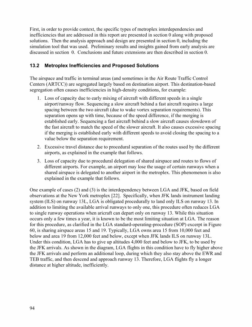
94

First, in order to provide context, the specific types of metroplex interdependencies and inefficiencies that are addressed in this report are presented in section 0 along with proposed solutions. Then the analysis approach and design are presented in section 0, including the simulation tool that was used. Preliminary results and insights gained from early analysis are discussed in section 0. Conclusions and future extensions are then described in section 0.

13.2 Metroplex Inefficiencies and Proposed Solutions The airspace and traffic in terminal areas (and sometimes in the Air Route Traffic Control Centers (ARTCC)) are segregated largely based on destination airport. This destination-based segregation often causes inefficiencies in high-density conditions, for example:

1. Loss of capacity due to early mixing of aircraft with different speeds in a single airport/runway flow. Sequencing a slow aircraft behind a fast aircraft requires a large spacing between the two aircraft (due to wake vortex separation requirements). This separation opens up with time, because of the speed difference, if the merging is established early. Sequencing a fast aircraft behind a slow aircraft causes slowdown of the fast aircraft to match the speed of the slower aircraft. It also causes excessive spacing if the merging is established early with different speeds to avoid closing the spacing to a value below the separation requirement.

2. Excessive travel distance due to procedural separation of the routes used by the different airports, as explained in the example that follows.

3. Loss of capacity due to procedural delegation of shared airspace and routes to flows of different airports. For example, an airport may lose the usage of certain runways when a shared airspace is delegated to another airport in the metroplex. This phenomenon is also explained in the example that follows.

One example of cases (2) and (3) is the interdependency between LGA and JFK, based on field observations at the New York metroplex [22]. Specifically, when JFK lands instrument landing system (ILS) on runway 13L, LGA is obligated procedurally to land only ILS on runway 13. In addition to limiting the available arrival runways to only one, this procedure often reduces LGA to single runway operations when aricraft can depart only on runway 13. While this situation occurs only a few times a year, it is known to be the most limiting situation at LGA. The reason for this procedure, as clarified in the LGA standard-operating-procedure (SOP) excerpt in Figure 60, is sharing airspace areas 15 and 19. Typically, LGA owns area 15 from 10,000 feet and below and area 19 from 12,000 feet and below, except when JFK lands ILS on runway 13L. Under this condition, LGA has to give up altitudes 4,000 feet and below to JFK, to be used by the JFK arrivals. As shown in the diagram, LGA flights in this condition have to fly higher above the JFK arrivals and perform an additional loop, during which they also stay above the EWR and TEB traffic, and then descend and approach runway 13. Therefore, LGA flights fly a longer distance at higher altitude, inefficiently.

95

Figure 60. Example of metroplex interdependency.

Two potential methods to help mitigate these types of inefficiencies are: Reducing the effect of speed mixing by segregating the traffic by speed where possible. Initial ideas of segregation by speed for a single airport were published in reference [23] Generalizing this approach to a metroplex environment, traffic may be segregated by speed as opposed to, or in addition to, by the destination airport. This setup is shown in Figure 61 notionally. For example, by using multiple parallel downwind and base leg segments, the fast aircraft (larger triangles) are assigned on outer downwind/base legs relative to the slower aircraft (smaller triangles), which are assigned on inner downwind/base legs. Airports are shown as crosses in the figure. Allowing sharing of approach segments (such as downwind and base legs) by arrivals to neighboring airports. This method can be combined with speed segregation where, for example, aircraft of the same speed category but heading to different airports are assigned on the same approach segments. An example is shown in Figure 61, where the fast aircraft heading to two different airports (blue and red large triangles) share a downwind leg.

96

Figure 61. Segregation by speed instead of by destination airport.

The hypothesized benefits of this approach include:

1. Increasing throughput by delaying the merging between slow and fast aircraft.

2. Increasing throughput by enabling the use of runways otherwise unused because of interdependencies. For example, LGA could use runways other than 13 (such as runway 4) when JFK is landing ILS on runway 13L, by sharing airspace areas 15 and 19 below 4000 feet with JFK. Flights for LGA and JFK would share approach segments in areas 15 and 19 and perform an exit to the respective airport/runway.

3. Increasing throughput and reducing travel distance by sharing of airspace and routes currently delegated procedurally to different airports. In the example, LGA flights landing on runway 13 could share airspace areas 19 and 15 below 4000 feet with the JFK arrivals to runway 13L. Then each could perform a late exit to the respective airport. If prioritization is needed, this sharing can be allowed for some of the LGA flights only when there is a lull in the JFK flow to runway 13L, thus reducing the longer and higher travel for at least some of the LGA flights.

It must be noted that such sharing methods require new controller procedures and possibly automation support. These requirements are not addressed in this report, which focuses mainly on making the benefit case.

13.3 Analysis Approach and Design This report presents preliminary experiments for proof of concept of the traffic organization approach described in the previous section. 13.3.1 Analysis Plan

The analysis compares the following scenarios:

97

Single airport

One approach path with mixed aircraft speeds (baseline)

Multiple approach paths with different speed category per path

Two airports One approach path for each airport with mixed aircraft speeds (baseline)

Sharing speed-based approach segments among the airports

The analysis compares the scenarios given in terms of the following metrics:

1. Throughput

2. Trajectory flexibility (explained in section 13.3.2) 13.3.2 Simulation Tool

The tool used for the analysis is a MATLAB simulation environment that was developed for trajectory flexibility planning in the presence of controlled arrival time and hazard/traffic avoidance constraints [24]. Trajectory flexibility is defined as the ability of a trajectory to accommodate disturbances while meeting constraints such as controlled time-of-arrival constraints and traffic-/hazard-avoidance constraints. Disturbances are events that pose risk of constraint violation, such as the uncertainty in the traffic/hazard dynamics. Relevant trajectory characteristics to measuring flexibility were identified; they included robustness and adaptability. Robustness is defined as the ability of a trajectory to remain feasible given disturbances, while adaptability is defined as the ability to regain feasibility if feasibility is lost because of disturbances. Details of formal mathematical definitions of these metrics and estimation techniques are given in reference [24]. The tool implements a dynamic programming approach to estimate the trajectory flexibility metrics and to use them (along with other objectives) for trajectory planning. These methods are described in reference [24]. Briefly, the method is based on discretizing space (currently only two dimensions) into square cells and time into steps. Then a solution space of all trajectories is built as a reachability tree connecting the resulting discrete nodes (each node represents a location as the center of a cell and time). The tree is based on reachability given discrete degrees of freedom (DOF), namely allowable speed and heading changes with discrete increments and within given ranges. At each node of the tree, adaptability is measured by the number of feasible trajectories that reach from that node to the destination (defined as a location with a time-of-arrival constraint). To estimate this number of feasible trajectories, a convolution process is used that starts at the destination and proceeds backwards, adding up feasible trajectories within the reachability bounds from each node. The convolution process is preceded at each time step by a filtering process that zeros out the number of trajectories at nodes that violate any constraints. The constraints include violation of separation from hazards and from other traffic or violation of time-of-arrival constraints at a node. After building the solution space tree with the metrics at each node, a trajectory is computed using a dynamic program that optimizes an objective function. For more details, see reference [24]. The objective function used in this preliminary analysis maximized adaptability at each node along the trajectory.

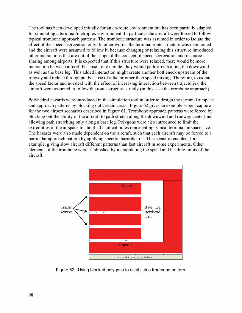
98

The tool has been developed initially for an en-route environment but has been partially adapted for simulating a terminal/metroplex environment. In particular the aircraft were forced to follow typical trombone approach patterns. The trombone structure was assumed in order to isolate the effect of the speed segregation only. In other words, the terminal route structure was maintained and the aircraft were assumed to follow it, because changing or relaxing this structure introduced other interactions that are out of the scope of the concept of speed segregation and resource sharing among airports. It is expected that if this structure were relaxed, there would be more interaction between aircraft because, for example, they would path stretch along the downwind as well as the base leg. This added interaction might create another bottleneck upstream of the runway and reduce throughput because of a factor other than speed mixing. Therefore, to isolate the speed factor and not deal with the effect of increasing interaction between trajectories, the aircraft were assumed to follow the route structure strictly (in this case the trombone approach). Polyhedral hazards were introduced in the simulation tool in order to design the terminal airspace and approach patterns by blocking out certain areas. Figure 62 gives an example screen capture for the two airport scenarios described in Figure 61. Trombone approach patterns were forced by blocking out the ability of the aircraft to path stretch along the downwind and runway centerline, allowing path stretching only along a base leg. Polygons were also introduced to limit the extremities of the airspace to about 50 nautical miles representing typical terminal airspace size. The hazards were also made dependent on the aircraft, such that each aircraft may be forced to a particular approach pattern by applying specific hazards to it. This scenario enabled, for example, giving slow aircraft different patterns than fast aircraft in some experiments. Other elements of the trombone were established by manipulating the speed and heading limits of the aircraft.

Figure 62. Using blocked polygons to establish a trombone pattern.

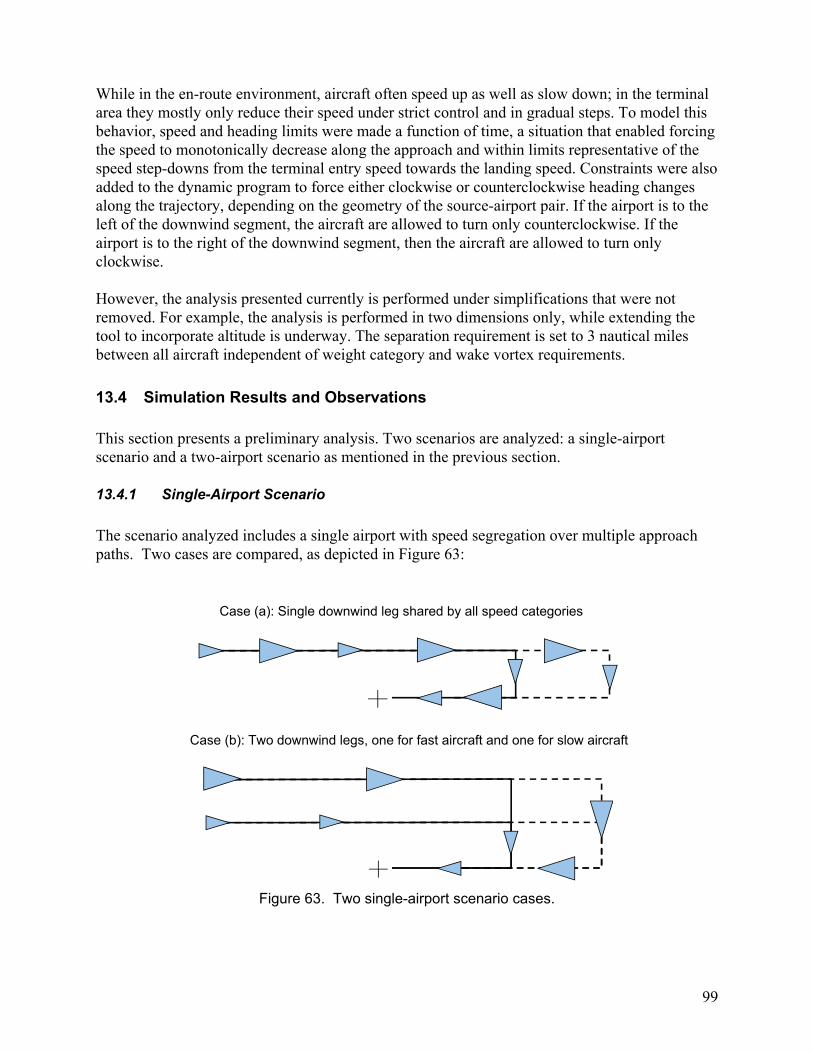
99

While in the en-route environment, aircraft often speed up as well as slow down; in the terminal area they mostly only reduce their speed under strict control and in gradual steps. To model this behavior, speed and heading limits were made a function of time, a situation that enabled forcing the speed to monotonically decrease along the approach and within limits representative of the speed step-downs from the terminal entry speed towards the landing speed. Constraints were also added to the dynamic program to force either clockwise or counterclockwise heading changes along the trajectory, depending on the geometry of the source-airport pair. If the airport is to the left of the downwind segment, the aircraft are allowed to turn only counterclockwise. If the airport is to the right of the downwind segment, then the aircraft are allowed to turn only clockwise. However, the analysis presented currently is performed under simplifications that were not removed. For example, the analysis is performed in two dimensions only, while extending the tool to incorporate altitude is underway. The separation requirement is set to 3 nautical miles between all aircraft independent of weight category and wake vortex requirements.

13.4 Simulation Results and Observations This section presents a preliminary analysis. Two scenarios are analyzed: a single-airport scenario and a two-airport scenario as mentioned in the previous section. 13.4.1 Single-Airport Scenario

The scenario analyzed includes a single airport with speed segregation over multiple approach paths. Two cases are compared, as depicted in Figure 63: Case (a): Single downwind leg shared by all speed categories

Case (b): Two downwind legs, one for fast aircraft and one for slow aircraft

Figure 63. Two single-airport scenario cases.

100

The scenario includes the following parameters:

• Two landing-speed categories are used: Fast with 120 knots and slow with 80 knots.

• Landing speed is met with 30-knot tolerance.

• Maximum demand is assumed available at all time (to determine maximum throughput).

• Aircraft speed categories are alternated in the demand stream to maximize the speed mix effect.

• To maximize throughput, the time of arrival (STA) is minimized for each aircraft using the following algorithm:

o For each aircraft i

Assign STA(i) = STA(i-1) + 1 minute

Increment entry time of aircraft i until STA(i) is met; if not met before entry time is larger than STA(i), then

Increment STA(i) by 1 minute and go to previous step.

To model speed step-down, the speed limits are set to [max min] = [210 170] until STA/2, then to [max min] = [170 landing-speed] until landing.

Separation requirement is set to 3 nautical miles, independent of the aircraft type.

Path stretching is allowed only using trombone of the base leg.

Time is discretized using 2-minute time increments, and space is discretized using 1 x 1 nautical mile square cells.

The spatial span of the scenario is 50 nautical miles. Throughput and trajectory flexibility (adaptability) were compared between cases (a) and (b). As shown in Figure 64, throughput was higher in case (b), segregating speed categories onto two trombones, than in case (a), which combined the two speed categories in one trombone. In this example the throughput was higher by about 20%. The 10 aircraft in the scenario landed in 1020 seconds in case (b) compared to 1320 in case (a). However, it should be noted that this analysis is a theoretical simulation that is not validated against current operations. Therefore, the increase in throughput should not be interpreted as a potential increase if such a procedure is adopted relative to current operations, since the baseline may be different and may include some degree of segregation by speed and delay of merging, to the extent practiced by controllers.

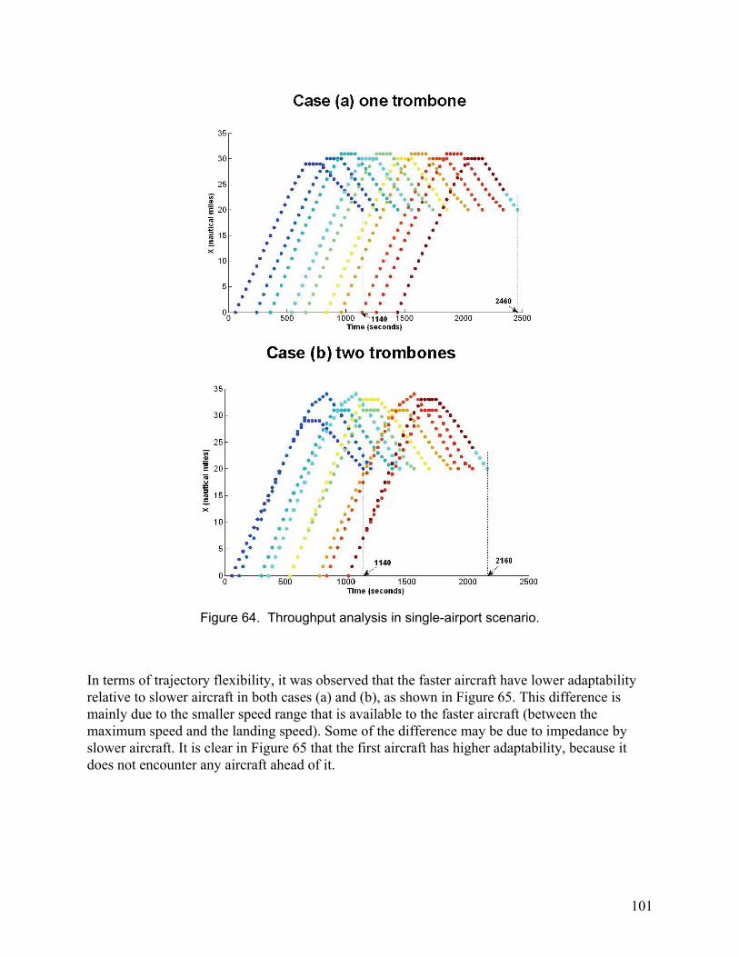
101

Figure 64. Throughput analysis in single-airport scenario.

In terms of trajectory flexibility, it was observed that the faster aircraft have lower adaptability relative to slower aircraft in both cases (a) and (b), as shown in Figure 65. This difference is mainly due to the smaller speed range that is available to the faster aircraft (between the maximum speed and the landing speed). Some of the difference may be due to impedance by slower aircraft. It is clear in Figure 65 that the first aircraft has higher adaptability, because it does not encounter any aircraft ahead of it.

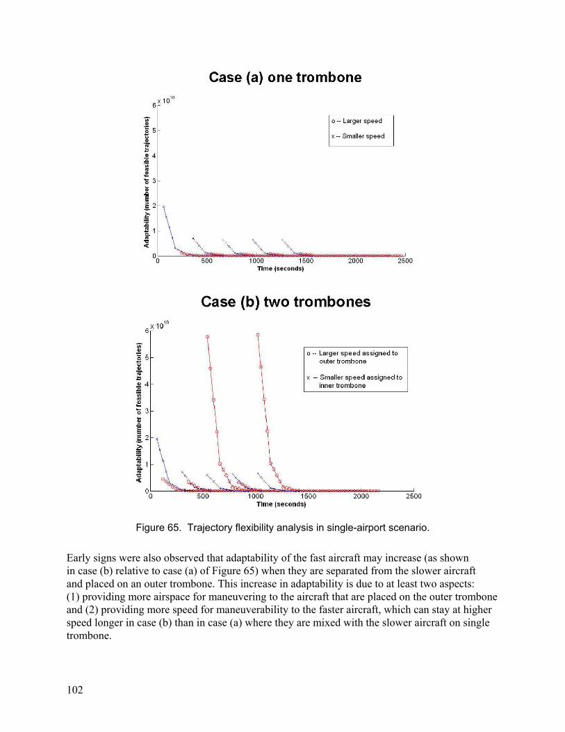
102

Figure 65. Trajectory flexibility analysis in single-airport scenario.

Early signs were also observed that adaptability of the fast aircraft may increase (as shown in case (b) relative to case (a) of Figure 65) when they are separated from the slower aircraft and placed on an outer trombone. This increase in adaptability is due to at least two aspects: (1) providing more airspace for maneuvering to the aircraft that are placed on the outer trombone and (2) providing more speed for maneuverability to the faster aircraft, which can stay at higher speed longer in case (b) than in case (a) where they are mixed with the slower aircraft on single trombone.

103

13.4.2 Two-Airport Scenario The scenario analyzed in this section includes two airports with speed segregation over multiple approach paths. Two cases are compared in Figure 66: Case (a): Each airport has a single downwind leg, shared by all speed categories heading to the airport. In this case the two airports operate independently with separate approach paths.

Case (b): The two airports use three downwind legs, two of which are dedicated to the

slow traffic of each of the airports, with each airport using the leg closer to it. The third central downwind leg is shared by the fast traffic heading to either airport.

Figure 66. Two two-airport scenario cases. The scenario includes the same parameters as in the single-airport scenario, where the aircraft speed categories are alternated in the demand stream for each airport to maximize the speed mix effect. They are also alternated between airports to maintain equal loads on the two airports. The STA is minimized for each aircraft (to maximize throughput) using the same algorithm. Time is discretized using 1-minute time increments and space is discretized using 1 x 1 nautical mile cells. Throughput and trajectory flexibility (adaptability) were compared between cases (a) and (b) in Figure 67 and Figure 68, respectively.

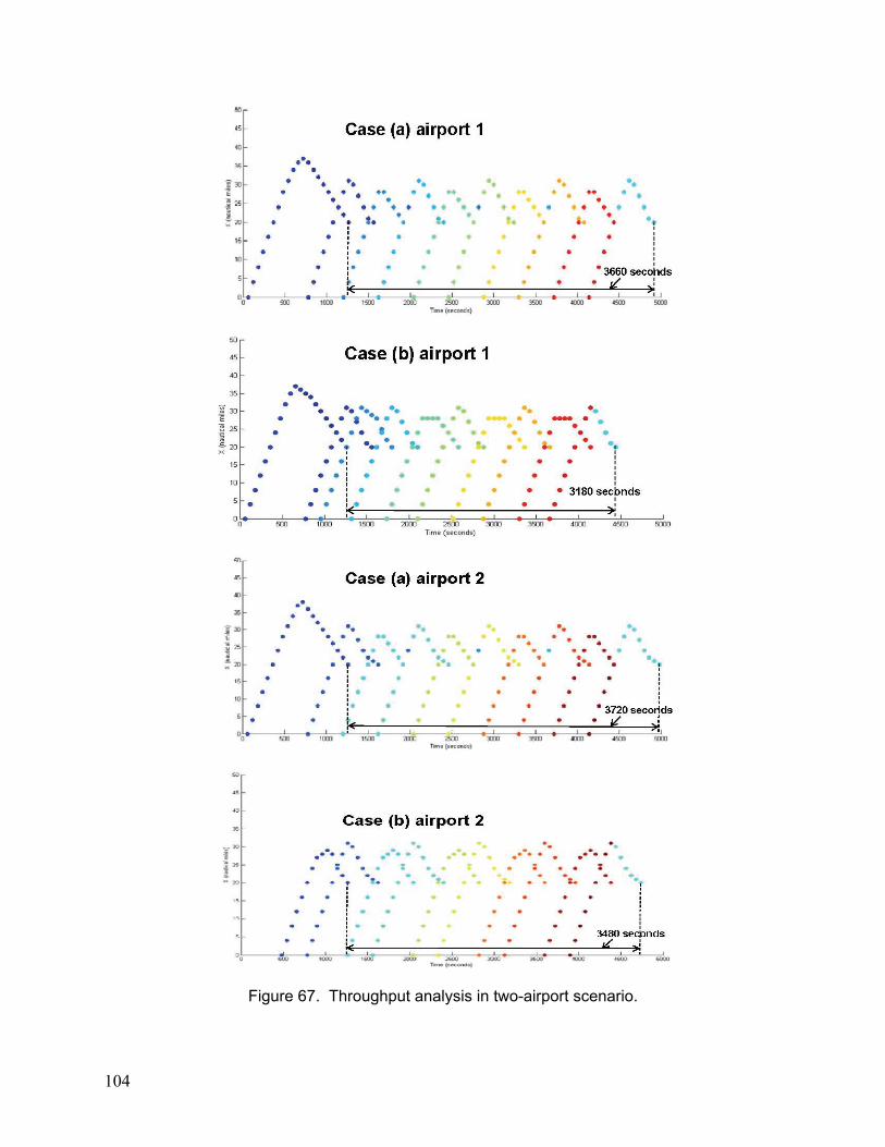
104

Figure 67. Throughput analysis in two-airport scenario.

105

As shown in Figure 67, throughput was higher in case (b), segregating speed categories onto two trombones with a shared central downwind for the fast aircraft, than in case (a), which combined the two speed categories in one trombone for each airport. In this example the throughput was higher by about 13% for the first airport and by about 6% for the second airport. The 10 aircraft landed in 480 seconds less for airport 1 and in 240 seconds less for airport 2, in case (b) compared to case (a). The difference between two airports is attributed mainly to the order in which the aircraft were introduced, which caused the second airport to lose some benefits because its first fast aircraft has to platoon behind the first fast aircraft heading to the first airport along the shared centerline. The gain is not as high as 20 percent, which was the gain of both airports if each had two independent trombones for its slow and fast aircraft without sharing resources with the other airport. The reduction in the gain is because while speed segregation increases throughput, the central downwind leg is shared between the two airports. Despite sharing, the speed segregation resulted in a throughput benefit in the range between 6 and 13%. Again, it should be noted that this analysis is a theoretical simulation that is not validated against current operations. Therefore, the increase in throughput should not be interpreted as a potential increase if such a procedure is adopted relative to current operations, since the baseline may be different and may include some degree of segregation by speed and delay of merging, to the extent practiced by controllers. It should also be noted that sharing the downwind segment enables other benefits that are not measured in this analysis—for example, enabling the airports to use additional runways or travel less distance, as described in section 11. In terms of trajectory flexibility, signs were also observed that adaptability of the fast aircraft may increase (as shown in Figure 68 in case (b) relative to case (a) for airport 1) when they are separated from the slower aircraft and placed on a separate downwind leg. The logarithm of adaptability (log of the number of feasible trajectories at each point) is plotted because adaptability grows exponentially with negative time. This increase in adaptability is due to at least two aspects: (1) providing more airspace for maneuvering to the aircraft that are placed on the outer trombone for each airport and (2) providing more speed for maneuverability to the faster aircraft, which can stay at higher speed longer in case (b) than in case (a) when they are mixed with the slower aircraft on single trombone. The gain in adaptability for the second airport is not as noticeable as for the first airport. One reason may be because of the order in which the aircraft are introduced. The fast aircraft of the second airport are introduced behind those of airport 1 on the shared downwind leg. This situation may have impeded the aircraft of airport 2 and resulted in less adaptability in addition to less throughput for airport 2. However, more analysis is needed to investigate the difference.

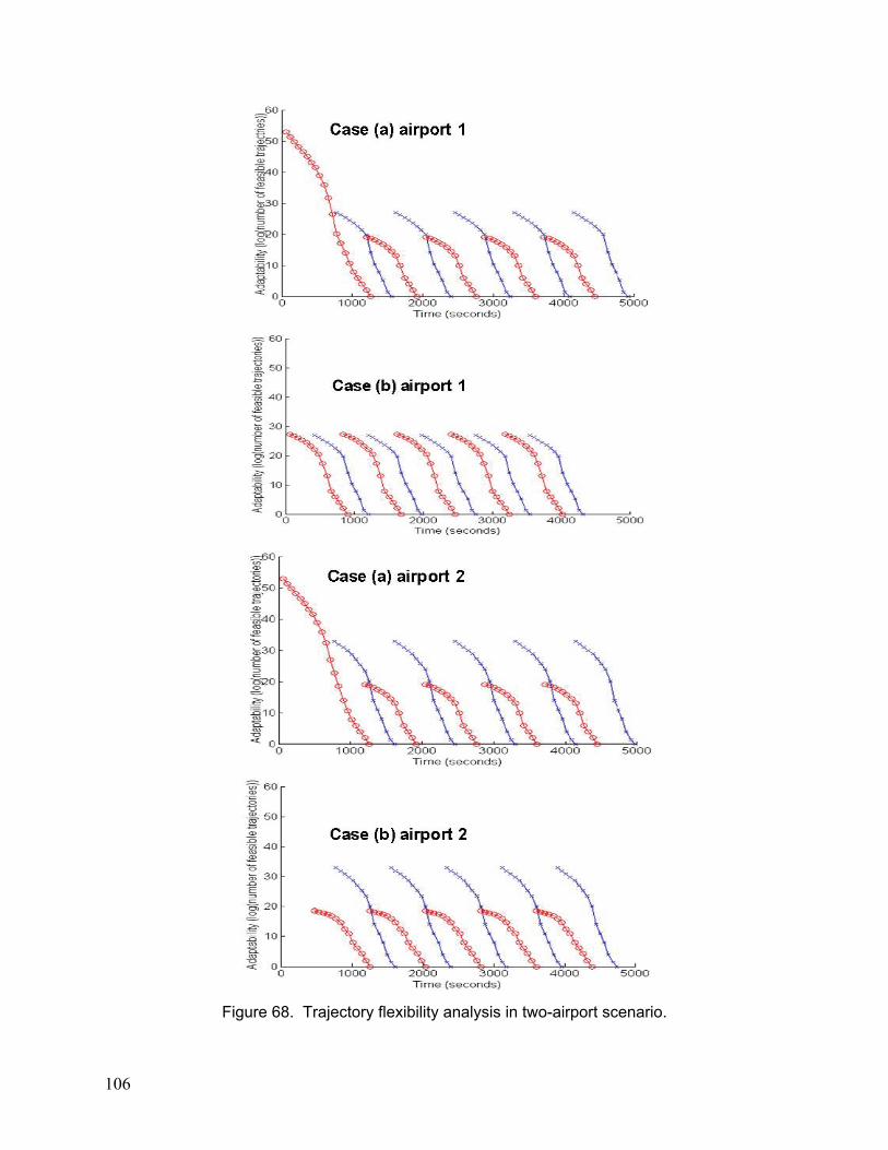
106

Figure 68. Trajectory flexibility analysis in two-airport scenario.

107

13.5 Conclusions

A preliminary analysis was described in this report as a proof of concept for organizing traffic in a metroplex based on speed segregation as opposed to (or in addition to) destination airport. This organization involved two techniques: (1) Sharing airspace and route resources among airports, thus opening up runway capacity and shortening travel distance and (2) segregating aircraft by speed, thus reducing the mixing between fast and slow aircraft in the same flow. This preliminary analysis demonstrated encouraging signs of benefiting from the solutions proposed. The benefits were demonstrated in terms of increasing throughput and trajectory flexibility, which allows better mitigation of the risk of constraint violation. For a single-airport scenario the theoretical increase in throughput was up to 20% because of speed segregation. For a two-airport scenario the increase in throughput was less, ranging between 6 and 13%, because of sharing resources between the two airports in addition to the speed segregation. The analysis presented in this report is preliminary, and further analysis of additional scenarios is needed. Future extensions of this research include validating the benefits by analyzing historic data and using a baseline that represents current operations in terms of the level of speed segregation that is practiced. Future research may also investigate the added benefits of increasing runway capacity and reducing travel distance because of sharing resources among airports more effectively than in current procedures.

14 AIRCRAFT MODELS

This section describes the aircraft models required as a part of the metroplex management solution approach. The aircraft models will be used in two ways. In the planning phase, the models will be used to provide feasible ranges of flight time along route segments and the associated cost function contributions. In the simulation phase, the models will introduce some error and possibly be given additional constraints along a route, such as required times at intersection points, and will be used to provide the actual aircraft motion. The predefined routes should be realistic. Therefore, we need the ability to define detailed routes between runways and fixes that aircraft are capable of following. We may use the aircraft models in advance to demonstrate that the routes are feasible. Note that the “aircraft models” from our perspective include not only the vehicle dynamics but also the vehicle control and guidance to follow defined routes. To support the planner, we need an aircraft model for an aircraft following a route where the route does not specify “longitudinal” motion (i.e., speed along the route). The aircraft model must include a model for the speed along the route. The aircraft model should represent aircraft turns as well as the vertical profile climbing and descending of the aircraft. When the route does not include vertical restrictions, or when it includes very loose restrictions, the aircraft model

108

should represent an efficient/optimal climb/descent profile. The output of the model will be information such as the fastest the aircraft can traverse the route (and the associated cost) and the slowest the aircraft can traverse the route (and the associated cost), so that the planner may plan separation at intersection points. In addition to a route, the planner may assign the aircraft required times (RTs), which may be a point in time at which the aircraft should cross the specified position or a time window during which the aircraft should cross the specified position at various points along the route, including the runway, fix, and points where routes intersect. The aircraft model should be able to comply with these RTs or provide an error if an RT is not achievable. Eventually, the aircraft model should have different models/parameters to represent different aircraft types. In this project, we used a single aircraft model. To support modeling what “actually” happens when aircraft try to follow the plan produced by the metroplex planner, the aircraft model should be able to vary the aircraft performance in complying with the route (in both lateral and vertical dimensions) and RTs. This capability will also be used to study the impact of aircraft navigation performance on metroplex management efficiency and airspace structure design. Simulating the “actual” result of the planner output also allows us to study a dynamic situation where the planner is confronted with the actual results of the prior plan and must produce a revised plan.

14.1 Aircraft Dynamics Model The three-dimensional point-mass equations of motion for an aircraft are considered adequate for route feasibility in terms of maintaining realistic aircraft physics, as well as providing state information for optimization purposes. The point mass equations of motion predominantly given in aircraft performance texts do not include wind effects, and also usually consider the thrust to be aligned with the velocity vector. While these assumptions are valid for preliminary analysis, as fuel-burn modeling accuracy becomes more crucial, the effects of winds and thrust direction with respect to the velocity vector also become more critical. With that said, the equations of motion and fuel burn, as given in reference [25], are slightly more detailed than typically found in undergraduate-level texts and are expressed as:

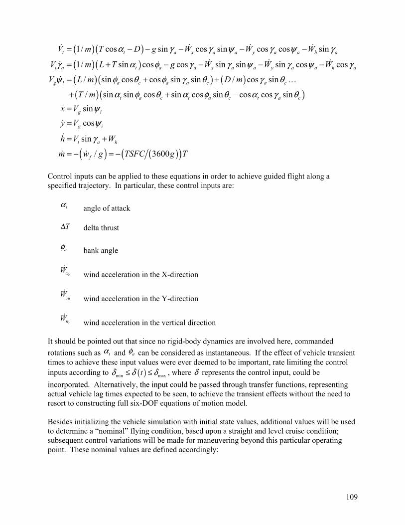
109

( )( )( )( )( )( ) ( )( )

1/ cos sin cos sin cos cos sin

1/ sin cos cos sin sin sin cos cos

/ sin cos cos sin sin / cos sin

/ sin sin cos sin

t t a x a a y a a h a

t a t a a x a a y a a h a

g i a c a a c a c

t a c t

V m T D g W W W

V m L T g W W W

V L m D m

T m

α γ γ ψ γ ψ γ

γ α φ γ γ ψ γ ψ γ

ψ φ θ φ γ θ γ θ

α φ θ α

= − − − − −

= + − − − −

= + +

+ +

( )

( ) ( )( )

cos sin cos cos sin

sin

cos

sin

/ 3600

a c t a c

g i

g i

t a h

f

x V

y V

h V W

m w g TSFC g T

φ θ α γ θψψ

γ

−=

=

= +

= − = −

Control inputs can be applied to these equations in order to achieve guided flight along a specified trajectory. In particular, these control inputs are:

tα angle of attack TΔ delta thrust

aφ bank angle

0xW wind acceleration in the X-direction

0yW wind acceleration in the Y-direction

0hW wind acceleration in the vertical direction

It should be pointed out that since no rigid-body dynamics are involved here, commanded

rotations such as tα and aφ can be considered as instantaneous. If the effect of vehicle transient times to achieve these input values were ever deemed to be important, rate limiting the control inputs according to ( )min maxtδ δ δ≤ ≤ , where δ represents the control input, could be

incorporated. Alternatively, the input could be passed through transfer functions, representing actual vehicle lag times expected to be seen, to achieve the transient effects without the need to resort to constructing full six-DOF equations of motion model. Besides initializing the vehicle simulation with initial state values, additional values will be used to determine a “nominal” flying condition, based upon a straight and level cruise condition; subsequent control variations will be made for maneuvering beyond this particular operating point. These nominal values are defined accordingly:

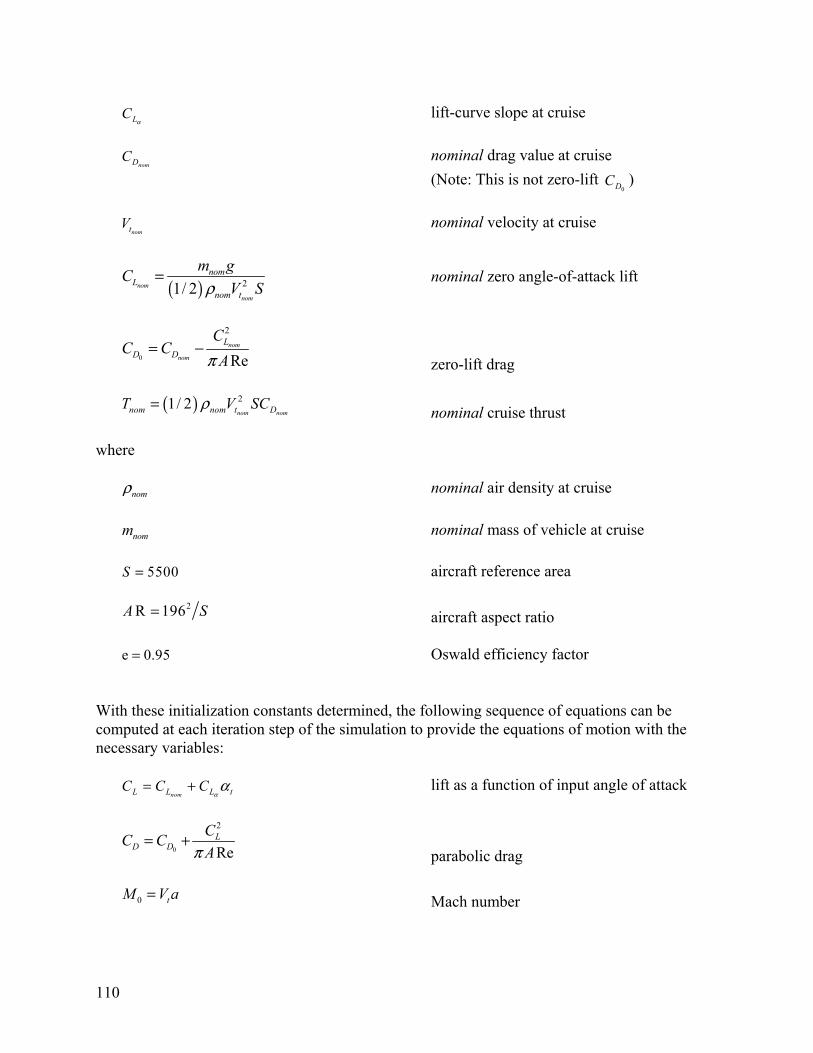
110

LC

α lift-curve slope at cruise

nomDC nominal drag value at cruise

(Note: This is not zero-lift 0DC )

nomtV nominal velocity at cruise

( ) 21/ 2nom

nom

nomL

nom t

m gC

V Sρ= nominal zero angle-of-attack lift

0

2

Renom

nom

LD D

CC C

Aπ= −

zero-lift drag

( ) 21/ 2nom nomnom nom t DT V SCρ=

nominal cruise thrust where nomρ nominal air density at cruise

nomm nominal mass of vehicle at cruise

5500S = aircraft reference area

2R 196A S= aircraft aspect ratio

e 0.95= Oswald efficiency factor With these initialization constants determined, the following sequence of equations can be computed at each iteration step of the simulation to provide the equations of motion with the necessary variables:

nomL L L tC C Cαα= +

lift as a function of input angle of attack

0

2

ReL

D D

CC C

Aπ= +

parabolic drag

0 tM V a= Mach number

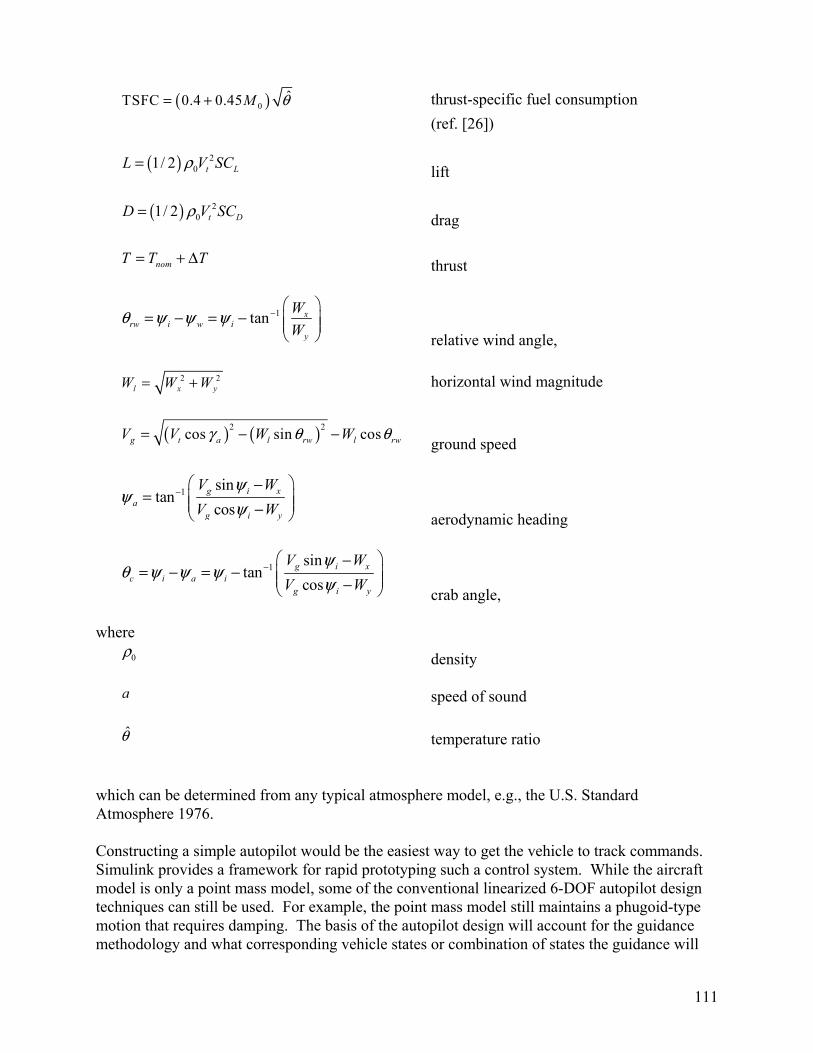
111

( )0ˆTSFC 0.4 0.45M θ= +

thrust-specific fuel consumption

(ref. [26])

( ) 201/ 2 t LL V SCρ=

lift

( ) 201/ 2 t DD V SCρ=

drag

nomT T T= + Δ thrust

1tan xrw i w i

y

W

Wθ ψ ψ ψ −

= − = − relative wind angle,

2 2

l x yW W W= +

horizontal wind magnitude

( ) ( )2 2

cos sin cosg t a l rw l rwV V W Wγ θ θ= − − ground speed

1 sintan

cosg i x

ag i y

V W

V W

ψψ

ψ− −

= − aerodynamic heading

1 sintan

cosg i x

c i a ig i y

V W

V W

ψθ ψ ψ ψ

ψ− −

= − = − − crab angle, where

0ρ density a speed of sound

θ̂ temperature ratio which can be determined from any typical atmosphere model, e.g., the U.S. Standard Atmosphere 1976. Constructing a simple autopilot would be the easiest way to get the vehicle to track commands. Simulink provides a framework for rapid prototyping such a control system. While the aircraft model is only a point mass model, some of the conventional linearized 6-DOF autopilot design techniques can still be used. For example, the point mass model still maintains a phugoid-type motion that requires damping. The basis of the autopilot design will account for the guidance methodology and what corresponding vehicle states or combination of states the guidance will

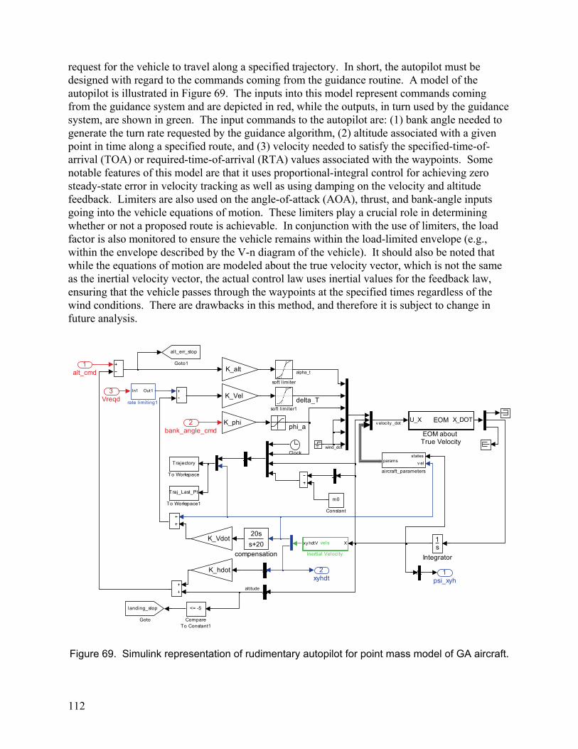
112

request for the vehicle to travel along a specified trajectory. In short, the autopilot must be designed with regard to the commands coming from the guidance routine. A model of the autopilot is illustrated in Figure 69. The inputs into this model represent commands coming from the guidance system and are depicted in red, while the outputs, in turn used by the guidance system, are shown in green. The input commands to the autopilot are: (1) bank angle needed to generate the turn rate requested by the guidance algorithm, (2) altitude associated with a given point in time along a specified route, and (3) velocity needed to satisfy the specified-time-of-arrival (TOA) or required-time-of-arrival (RTA) values associated with the waypoints. Some notable features of this model are that it uses proportional-integral control for achieving zero steady-state error in velocity tracking as well as using damping on the velocity and altitude feedback. Limiters are also used on the angle-of-attack (AOA), thrust, and bank-angle inputs going into the vehicle equations of motion. These limiters play a crucial role in determining whether or not a proposed route is achievable. In conjunction with the use of limiters, the load factor is also monitored to ensure the vehicle remains within the load-limited envelope (e.g., within the envelope described by the V-n diagram of the vehicle). It should also be noted that while the equations of motion are modeled about the true velocity vector, which is not the same as the inertial velocity vector, the actual control law uses inertial values for the feedback law, ensuring that the vehicle passes through the waypoints at the specified times regardless of the wind conditions. There are drawbacks in this method, and therefore it is subject to change in future analysis.

Figure 69. Simulink representation of rudimentary autopilot for point mass model of GA aircraft.

2xyhdt

1psi_xyh

soft limiter1

soft l imiter

In1 Out1

rate limiting1

20s

s+20

compensation

states

v elparams

aircraft_parameters

Traj_Last_Pt

To Workspace1

Trajectory

To Workspace

UY

UY

UY

UY

UY

1s

Integrator

Xxy hdtV vels

Inertial Velocity

alt_err_stop

Goto1

landing_stop

Goto

K_phi

K_Vdot

K_hdot

K_alt

K_Vel

U_X X_DOTEOM

EOM about True Velocity

m0

Constant

<= -5

CompareTo Constant1

Clock

3Vreqd

2bank_angle_cmd

1alt_cmd

v elocity _dotphi_a

delta_T

altitude

wind_dot

alpha_t

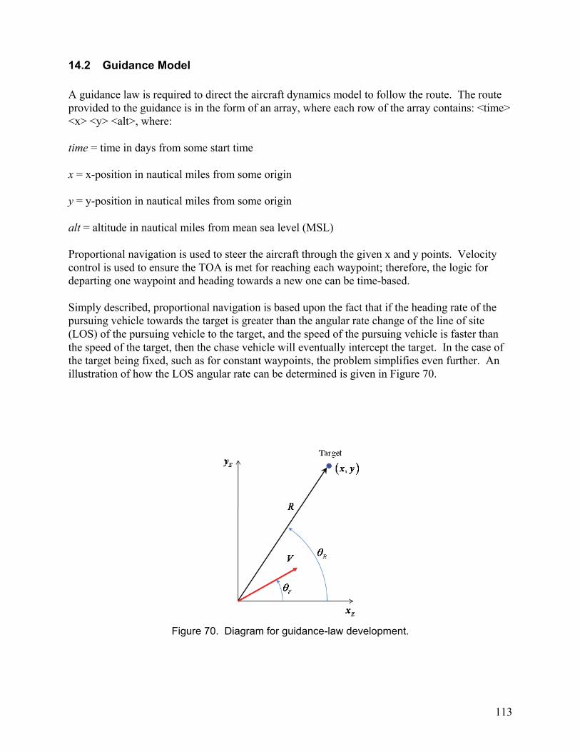
113

14.2 Guidance Model A guidance law is required to direct the aircraft dynamics model to follow the route. The route provided to the guidance is in the form of an array, where each row of the array contains: <time> <x> <y> <alt>, where: time = time in days from some start time x = x-position in nautical miles from some origin y = y-position in nautical miles from some origin alt = altitude in nautical miles from mean sea level (MSL) Proportional navigation is used to steer the aircraft through the given x and y points. Velocity control is used to ensure the TOA is met for reaching each waypoint; therefore, the logic for departing one waypoint and heading towards a new one can be time-based. Simply described, proportional navigation is based upon the fact that if the heading rate of the pursuing vehicle towards the target is greater than the angular rate change of the line of site (LOS) of the pursuing vehicle to the target, and the speed of the pursuing vehicle is faster than the speed of the target, then the chase vehicle will eventually intercept the target. In the case of the target being fixed, such as for constant waypoints, the problem simplifies even further. An illustration of how the LOS angular rate can be determined is given in Figure 70.

Figure 70. Diagram for guidance-law development.

114

By examining Figure 70, it should be clear that ( )VRV θθ −sin would represent the velocity that

is normal to the LOS vector, which is also equivalent to RRθ− , and therefore we can write the equation for the angular rate of the LOS vector as:

( )sin R VR

V

R

θ θθ

−= −

As stated, as long as the heading rate, Vθ , is greater than the angular rate of the LOS vector, Rθ ,

then the pursuing vehicle will be on a collision course with the target. Because heading rate, Vθ ,

is a function of velocity, V, and bank angle, aφ , then a required bank angle command, cmdφ , can

be determined based upon a desired vehicle heading, desV _θ , according to:

_1tan V descmd

V

g

θφ −

=

The bank angle command is one of the three inputs into the autopilot. The other two are the velocity command, which is generated based upon the current range to the target along with the time left to reach the target, and the altitude command, which comes straight from the route input array defined earlier. An example of the guidance law integrated with the autopilot and aircraft is given in Figure 71.

Figure 71. Integrated guidance with the autopilot and aircraft.

max(route_time)

2-D T[k]

Waypointsprevious

2-D T[k]

Waypointscurrent

1-D T[k]

Vel_cmd

1-D T[k]

TOASim Stopper

last_wp_stop

Goto1

PN_in PN_outPro_Nav_Plus

GUIDANCE LAW

1

[route_vel(length(route_vel)), size( route_pos,2)]

1

Clock

alt_cmd

bank_angle_cmd

Vreqd

psi_xyh

xyhdt

AUTOPILOT/AIRCRAFT

TGO

way points

old way points

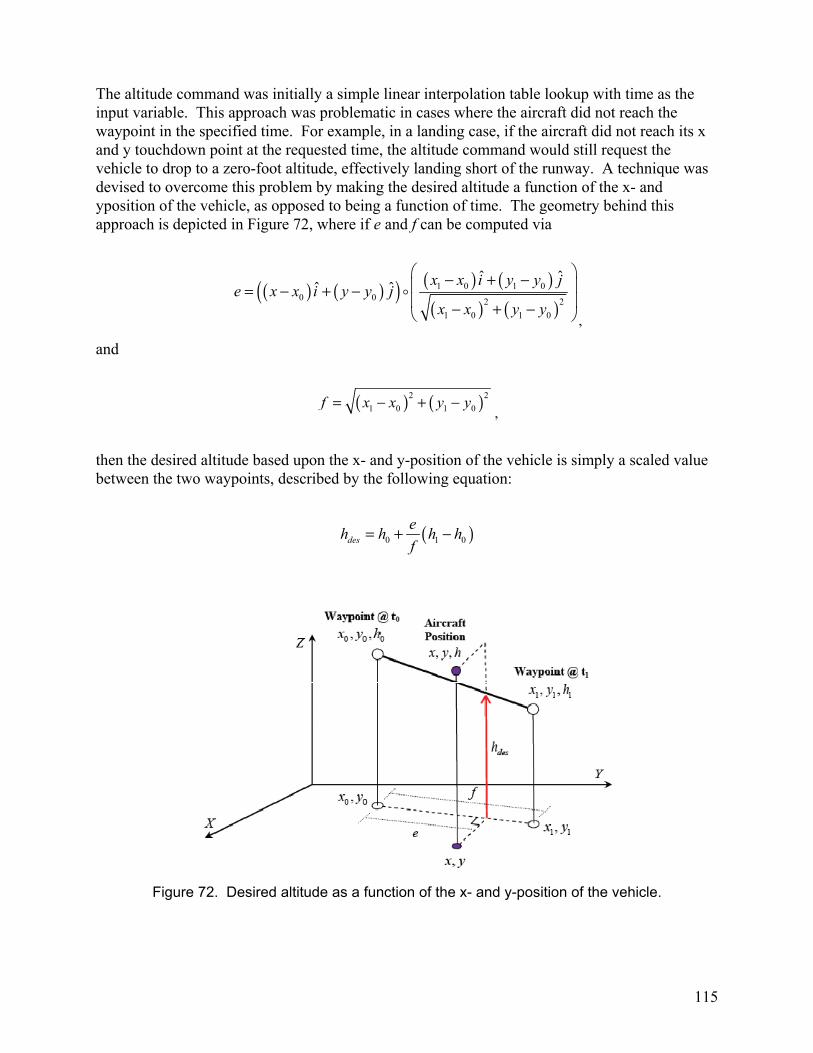
115

The altitude command was initially a simple linear interpolation table lookup with time as the input variable. This approach was problematic in cases where the aircraft did not reach the waypoint in the specified time. For example, in a landing case, if the aircraft did not reach its x and y touchdown point at the requested time, the altitude command would still request the vehicle to drop to a zero-foot altitude, effectively landing short of the runway. A technique was devised to overcome this problem by making the desired altitude a function of the x- and yposition of the vehicle, as opposed to being a function of time. The geometry behind this approach is depicted in Figure 72, where if e and f can be computed via

( ) ( )( ) ( ) ( )( ) ( )

1 0 1 00 0 2 2

1 0 1 0

ˆ ˆˆ ˆ x x i y y j

e x x i y y jx x y y

− + − = − + − − + −

,

and

( ) ( )2 2

1 0 1 0f x x y y= − + −,

then the desired altitude based upon the x- and y-position of the vehicle is simply a scaled value between the two waypoints, described by the following equation:

( )0 1 0des

eh h h h

f= + −

Figure 72. Desired altitude as a function of the x- and y-position of the vehicle.

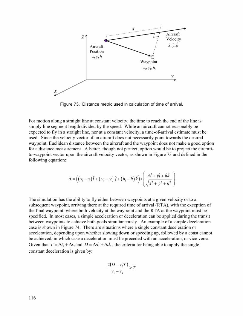
116

Figure 73. Distance metric used in calculation of time of arrival. For motion along a straight line at constant velocity, the time to reach the end of the line is simply line segment length divided by the speed. While an aircraft cannot reasonably be expected to fly in a straight line, nor at a constant velocity, a time-of-arrival estimate must be used. Since the velocity vector of an aircraft does not necessarily point towards the desired waypoint, Euclidean distance between the aircraft and the waypoint does not make a good option for a distance measurement. A better, though not perfect, option would be to project the aircraft-to-waypoint vector upon the aircraft velocity vector, as shown in Figure 73 and defined in the following equation:

( ) ( ) ( )( )1 1 1 2 2 2

ˆˆ ˆˆˆ ˆ xi yj hk

d x x i y y j h h kx y h

+ + = − + − + − + +

The simulation has the ability to fly either between waypoints at a given velocity or to a subsequent waypoint, arriving there at the required time of arrival (RTA), with the exception of the final waypoint, where both velocity at the waypoint and the RTA at the waypoint must be specified. In most cases, a simple acceleration or deceleration can be applied during the transit between waypoints to achieve both goals simultaneously. An example of a simple deceleration case is shown in Figure 74. There are situations where a single constant deceleration or acceleration, depending upon whether slowing down or speeding up, followed by a coast cannot be achieved, in which case a deceleration must be preceded with an acceleration, or vice versa. Given that 21 ttT Δ+Δ= and 21 ddD Δ+Δ= , the criteria for being able to apply the single constant deceleration is given by:

( )T

vv

TvD >−−

21

22

1 1 1, ,x y h

, ,x y h

X

Y

Z

Waypoint

Aircraft Position

Aircraft Velocity

d

, ,x y h

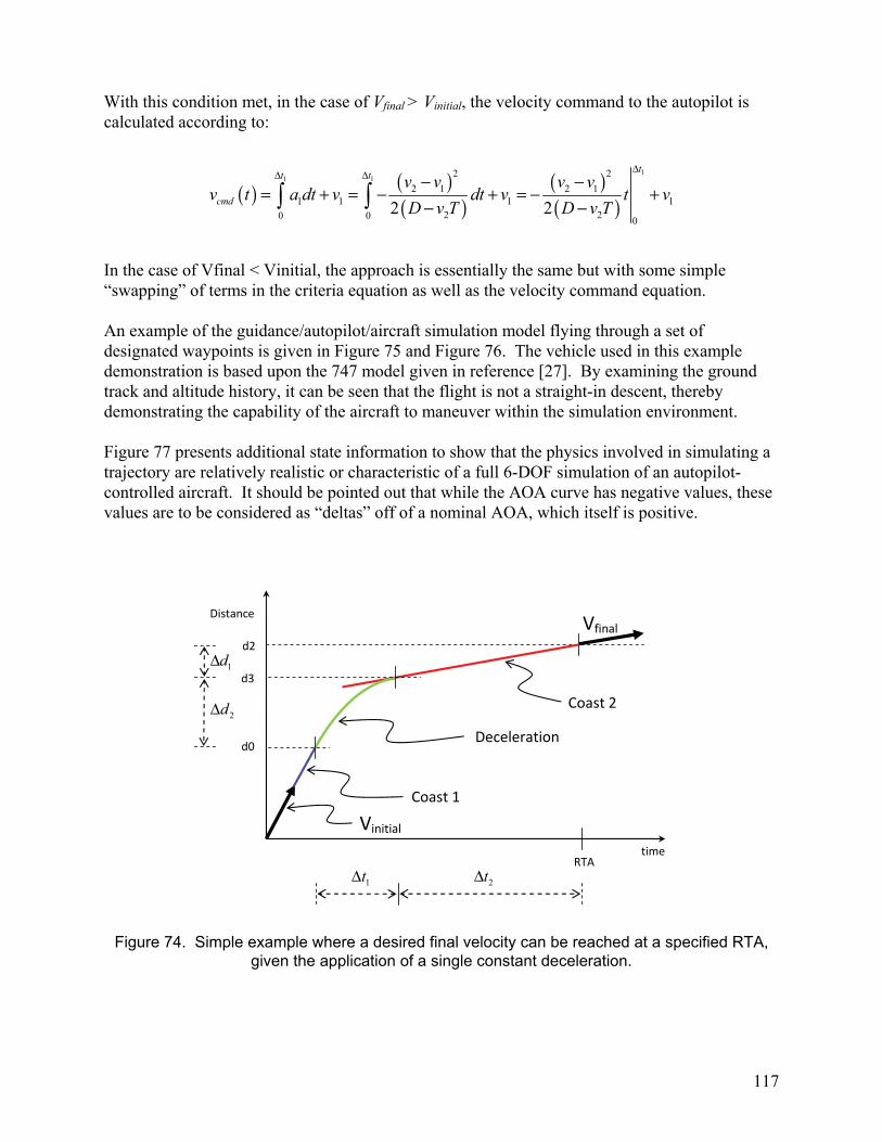
117

With this condition met, in the case of Vfinal > Vinitial, the velocity command to the autopilot is calculated according to:

( ) ( )( )

( )( )

11 1

2 2

2 1 2 11 1 1 1

2 20 0 02 2

tt t

cmd

v v v vv t a dt v dt v t v

D v T D v T

ΔΔ Δ − −

= + = − + = − +− −

In the case of Vfinal < Vinitial, the approach is essentially the same but with some simple “swapping” of terms in the criteria equation as well as the velocity command equation. An example of the guidance/autopilot/aircraft simulation model flying through a set of designated waypoints is given in Figure 75 and Figure 76. The vehicle used in this example demonstration is based upon the 747 model given in reference [27]. By examining the ground track and altitude history, it can be seen that the flight is not a straight-in descent, thereby demonstrating the capability of the aircraft to maneuver within the simulation environment. Figure 77 presents additional state information to show that the physics involved in simulating a trajectory are relatively realistic or characteristic of a full 6-DOF simulation of an autopilot-controlled aircraft. It should be pointed out that while the AOA curve has negative values, these values are to be considered as “deltas” off of a nominal AOA, which itself is positive.

Figure 74. Simple example where a desired final velocity can be reached at a specified RTA, given the application of a single constant deceleration.

RTA time

Distance

d2

d0

Vinitial

Vfinal

d3 1dΔ

2dΔ

1tΔ 2tΔ

Deceleration

Coast 1

Coast 2

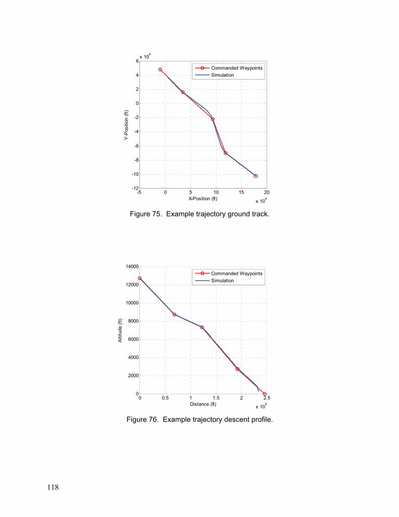
118

Figure 75. Example trajectory ground track.

Figure 76. Example trajectory descent profile.

-5 0 5 10 15 20

x 104

-12

-10

-8

-6

-4

-2

0

2

4

6x 10

4

X-Position (ft)

Y-P

ositi

on (

ft)

Commanded Waypoints

Simulation

0 0.5 1 1.5 2 2.5

x 105

0

2000

4000

6000

8000

10000

12000

14000

Distance (ft)

Alti

tude

(ft

)

Commanded Waypoints

Simulation

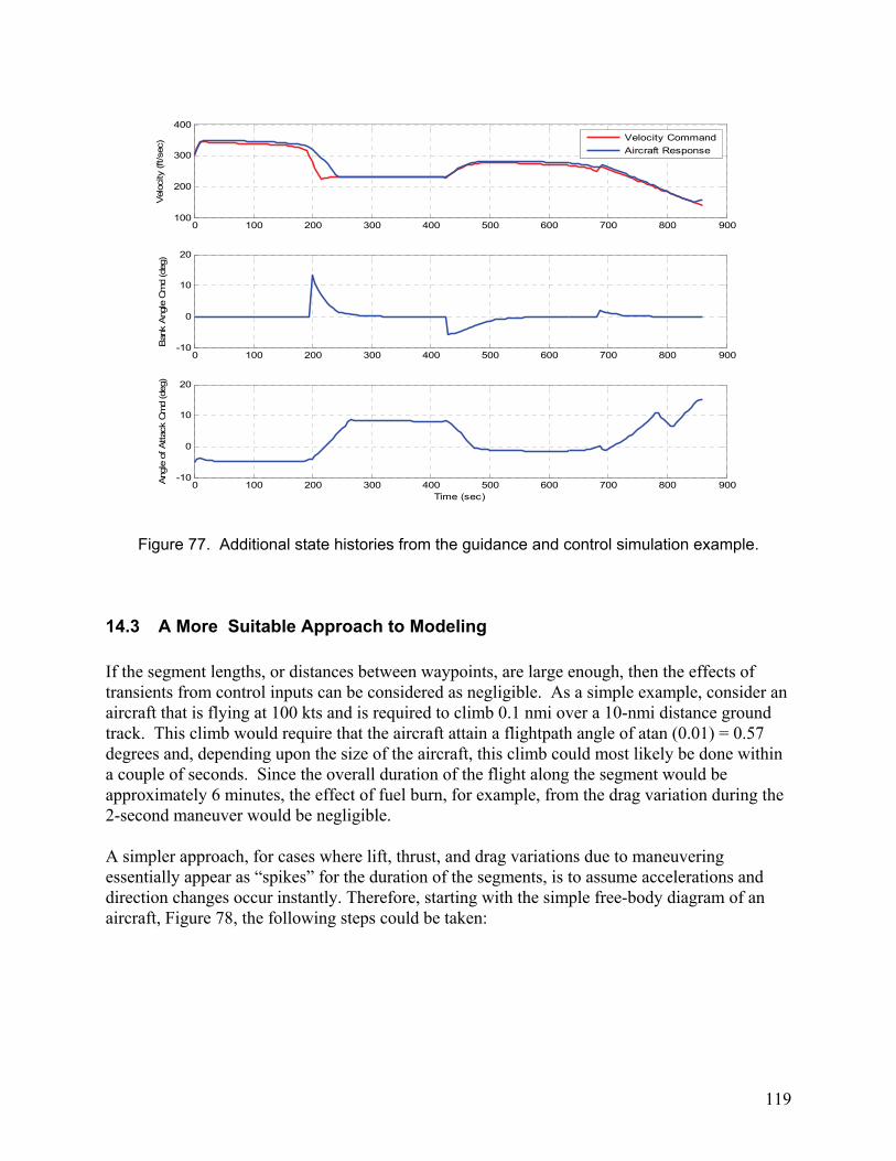
119

Figure 77. Additional state histories from the guidance and control simulation example.

14.3 A More Suitable Approach to Modeling If the segment lengths, or distances between waypoints, are large enough, then the effects of transients from control inputs can be considered as negligible. As a simple example, consider an aircraft that is flying at 100 kts and is required to climb 0.1 nmi over a 10-nmi distance ground track. This climb would require that the aircraft attain a flightpath angle of atan (0.01) = 0.57 degrees and, depending upon the size of the aircraft, this climb could most likely be done within a couple of seconds. Since the overall duration of the flight along the segment would be approximately 6 minutes, the effect of fuel burn, for example, from the drag variation during the 2-second maneuver would be negligible. A simpler approach, for cases where lift, thrust, and drag variations due to maneuvering essentially appear as “spikes” for the duration of the segments, is to assume accelerations and direction changes occur instantly. Therefore, starting with the simple free-body diagram of an aircraft, Figure 78, the following steps could be taken:

0 100 200 300 400 500 600 700 800 900100

200

300

400

Vel

ocity

(ft/s

ec)

Velocity Command

Aircraft Response

0 100 200 300 400 500 600 700 800 900-10

0

10

20

Ban

k A

ngle

Cm

d (d

eg)

0 100 200 300 400 500 600 700 800 900-10

0

10

20

Time (sec)

Ang

le o

f A

ttac

k C

md

(deg

)

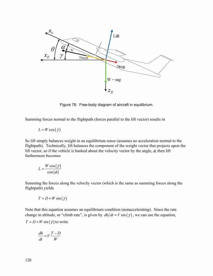
120

Figure 78. Free-body diagram of aircraft in equilibrium. Summing forces normal to the flightpath (forces parallel to the lift vector) results in

( )cosL W γ=

So lift simply balances weight in an equilibrium sense (assumes no acceleration normal to the flightpath). Technically, lift balances the component of the weight vector that projects upon the lift vector, so if the vehicle is banked about the velocity vector by the angle, φ, then lift furthermore becomes

( )( )

cos

cos

WL

γφ

=

Summing the forces along the velocity vector (which is the same as summing forces along the flightpath) yields

( )sinT D W γ= +

Note that this equation assumes an equilibrium condition (nonaccelerating). Since the rate change in altitude, or “climb rate”, is given by ( )sindh dt V γ= , we can use the equation,

( )sinT D W γ= + to write

dh T D

Vdt W

−=

121

But, recall that drag, D, varies parabolically with lift, L; hence, if lift is known, along with the aerodynamic parameters such as the wing aspect ratio, AR, and efficiency factor, e, then drag can be estimated. So, aircraft climb rate along a section between waypoints is primarily controlled by varying velocity, V, and thrust, T. Turn rate would be controlled by φ, but if instant acceleration is assumed to occur at the waypoints, then bank angles would not be necessary. As an example, from the estimation of thrust, as well as velocity along a segment, the fuel burn could be determined analytically, via the thrust-specific fuel consumption (TSFC). More specifically, it could be calculated almost instantly for a given segment without the need to resort to modeling and numerically solving the vehicle equations of motion. As an example, consider the following points in three-dimensional (3-D) space shown in Figure 79. For the case where acceleration along a segment is not permissible, the user can either select velocities, Vs along the segments, or specify times of arrival for the waypoints. Recall that a specified time of arrival (TOA) can be considered as synonymous with required time of arrival (RTA). If specified TOAs are preferred, then the velocity for each leg is simply the distance of the segment divided by the difference in the TOAs for the two waypoints that define the segment,

( ) ( ) ( )

01

201

201

201

RTARTA

zzyyxxV

−−+−+−

=

Figure 79. Analytical results can be calculated on a discrete per-segment basis.

122

Furthermore, the rate of climb can also be determined from Figure 79 and

( )( ) ( ) ( )2

012

012

01

01

zzyyxx

zzV

dt

dt

−+−+−

−=

Finally, the equation for drag is expressed as

( )2

22

21 1

Re

20 VSA

WVSCD D

+=

ρπρ

where

factor efficiency wing

ratioaspect wing

weight vehicle

area surface wing

densityair

drag profile 0

==

===

=

e

AR

W

S

CD

ρ

With these latter parameters all known for a given aircraft, e.g., from base of aircraft data (BADA) we have everything that we need to calculate the required thrust, T, along a segment, in turn providing us with a means to check if the vehicle is capable of achieving the desired velocity and thrust, hence allowing the path planning to determine whether or not selected paths are feasible. Additionally, the fuel burn along a segment can be estimated according to the TSFC, allowing optimal fuel-burn paths to be determined:

Tg

TSFCm

3600−=

123

15 CONCLUSIONS

15.1 Summary Being a metroplex is not binary—all regions will exhibit some metroplex phenomena since there are always at least a few small airports near a large airport. Therefore, traffic management solutions will not be either “metroplex” or “not metroplex.” Metroplex research needs to influence and be absorbed into system solutions so that metroplex solutions are not distinct approaches but additional elements to other Next-Generation Air Transportation System (NextGen) solutions. Similar to designing to handle bad weather or off-nominal situations, metroplex phenomena should be considered from the beginning, not after a single-airport solution has been finished. Metroplexes are unique. Metroplex phenomena will increase if instrument-flight-rules (IFR) traffic increases at regional airports or if NextGen changes operations at closely spaced large airports to increase operational flexibility and efficiency. For example, CDA approaches to Oakland (OAK) will require increased coordination with San Francisco (SFO) arrivals. This two-year project accomplished each of the original goals:

• Developed a solid understanding of the nature of metroplexes

• Examined a variety of frameworks for discussing and measuring metroplexes

• Decomposed the metroplex management problem into sub-problems consistent with other NextGen concepts

• Formulated and solved a generic optimal route selection/scheduling problem

o Studied a range of problem formulations to understand advantages and disadvantages

o Introduced and studied a variety of heuristics and methods for enabling faster solutions while retaining practical optimality

Developed an understanding of the relationship between metroplex characteristics and solution methods

Showed compatibility between our metroplex management solution and the single-airport super-dense operations problem

Developed a metroplex modeling capability that NASA has reused to support other research efforts

Published or otherwise disseminated all of our research findings Most significant, beyond our fundamental understanding of metroplex phenomena was our development of an optimization-based metroplex planning algorithm. This algorithm plans both route/resource assignments and scheduling at conflict points (i.e., shared resources). As such, this algorithm is a powerful tool for studying many traffic management problems. We are already reusing the basic algorithm to facilitate research in the System Oriented Runway Management (SORM) project, and NASA is using the algorithm and metroplex modeling environment to support super-density operations (SDO) research.

124

15.2 Future Work Study Application to Large-Scale Problems and Diverse Metroplex Environments The current project focused on developing a basic and thorough understanding of metroplex issues by studying small problems in detail. One future goal is to study full-sized problems across a wide variety of metroplex environments to ensure solution approaches scale (i.e., remain feasible to apply) and are sufficiently flexible to handle a broad set of metroplex phenomena and diverse combinations of simultaneous phenomena. We repeatedly considered each of these issues as we employed sample problems. However, demonstrating applicability to large, diverse problems is still required as proof. Develop Dynamic, Automatic Metroplex Airspace Design The current project assumed known airspace designs. By studying alternative designs, we provided important insight into how airspace design affects the metroplex problem and nature of the solution. This initial work suggested that metroplex airspace design is an important element of metroplex management. Moreover, dynamically adjusting the airspace structure in response to characteristics of the traffic demand and, of course, weather, may provide additional benefit. Furthermore, manually designing metroplex airspace structures proved time-consuming and difficult to do well. This reality, therefore, presents a challenge to applying our algorithms to many full-scale problems. Consequently, two future objectives are to 1) develop an automatic capability to calculate efficient metroplex airspace structures and 2) study dynamic metroplex airspace structure as a traffic management approach that takes advantage of more flexible (and performance-based) Next-Generation Air Transportation System (NextGen) airspace. Integrate with Other NextGen Concepts In designing our metroplex management approach, we considered NASA’s existing concept for operations within NextGen terminal airspace to ensure our concept would be compatible. A final future goal is to more explicitly study the integration of metroplex management techniques within other research areas, such as super-dense operations, airport surface traffic management, and traffic flow management optimization.

125

16 REFERENCES

1. Stephen Atkins, Stephen: Observation and Measurement of Metroplex Phenomena. IEEE Digital Avionics Systems Conference, St. Paul, Minn., 2008.

2. Capozzi, B.J.; Atkins, S.C.; and Choi, S.: Towards Optimal Routing and Scheduling of Metroplex Operations. 9th AIAA Aviation Technology, Integration, and Operations Conference, Hilton Head, S.C., 2009.

3. Idris, Husni: Queuing Analysis of Interdependencies between Multiple-Airport System Operations. AIAA ATIO Conference, 2009.

4. Idris, Husni: Queuing Analysis of Interdependencies in Airport Surface and Metroplex Operations. ICNS (presentation only), 2009.

5. Atkins, Stephen; and Idris, Husni: Literature Survey Report, Investigating the Nature of and Methods for Managing Metroplex Operations, NASA Contract NNA07BC56C, November 19, 2007.

6. Atkins, Stephen: Initial Site Survey Report, Investigating the Nature of and Methods for Managing Metroplex Operations. NASA Contract NNA07BC56C, December 14, 2007.

7. Atkins, Stephen: Observations of Metroplex Phenomena. Presentation at NASA Airspace Systems Program Technical Interchange Meeting, Austin, Tex., March 19, 2008.

8. Joint Planning and Development Office: Concept of Operations for the Next Generation Air Transportation System. v2.0, June 13, 2007.

9. Atkins, Stephen: Metroplex Definition Report, Investigating the Nature of and Methods for Managing Metroplex Operations. NASA Contract NNA07BC56C, April 30, 2008.

10. Atkins, Stephen: Metroplex Definition and Modeling. Presentation at NASA Airspace Systems Program Metroplex Workshop. Atlanta, Ga., September 10, 2008.

11. Atkins, Stephen; et al.: Metroplex Modeling Report, Investigating the Nature of and Methods for Managing Metroplex Operations. NASA Contract NNA07BC56C, March 10, 2009.

12. Atkins, Stephen; and Brian Capozzi: Metroplex Modeling and Traffic Management. Presentation at NASA Airspace Systems Program Metroplex Workshop, Atlanta, Ga., February 26, 2009.

13. Rathinam, S.; Montoya, J.; and Jung, Y.: An Optimization Model for Reducing Aircraft Taxi Times at the Dallas Fort Worth International Airport. 26th International Congress of the Aeronautical Sciences, 2008.

14. Atkins, Stephen; et al.: Initial Report on Metroplex Management Concepts, Investigating the Nature of and Methods for Managing Metroplex Operations. NASA Contract NNA07BC56C, May 29, 2009.

15. Atkins; Stephen; Capozzi, Brian; and Seongim Choi: Towards Optimal Route Assignment and Scheduling of Metroplex Traffic. Presentation at NASA Airspace Systems Program Technical Interchange Meeting, San Antonio, Tex., October 13, 2009.

126

16. Marin, A.: Airport Management: Taxi Planning. Annals of Operations Research, vol. 143, 2006, pp. 191–202.

17. Roling, P.; and Visser, H.: Optimal Airport Surface Traffic Planning Using Mixed-Integer Linear Programming. Intl. J. Aerospace Engineering, 2008.

18. Smeltink, J.; Soomer, M.; DeWaal, P.; and Van Der Mei, R.: An Optimisation Model for Airport Taxi Scheduling. Thirtieth Conference on the Mathematics of Operations Research. Lunteren, The Netherlands, 2005.

19. Keith, G.; Richards, A.; and Sharma, S.: Optimization of Taxiway Routing and Runway Scheduling. AIAA Guidance, Navigation and Control Conference and Exhibit. Honolulu, Hawaii, 2008.

20. Bemporad, A.; and Morari, A.: Control of Systems Integrating Logic, Dynamics, and Constraints. 2008.

21. Joint Planning and Development Office: Next Generation Air Transportation System Integrated Plan. URL: http://www.jpdo.gov/library/NGATS_v1_1204r.pdf

22. Atkins, S.: New York Metroplex Site Visit Report. NASA Report submitted by Mosaic ATM inc., 2008.

23. Idris, H.R.; and Simpson R.W.: New Approach to the Planning and Control of Air Traffic in the Terminal Area. Presented at the AIAA Guidance, Navigation and Control Conference, Boston, Mass., August 10–12, 1998.

24. Idris, H.; Delahaye, D.; and Wing, D.: Distributed Trajectory Flexibility Preservation for Traffic Complexity Mitigation, Proceedings of 8th USA/Europe Air Traffic Management R&D Seminar, Napa Valley, Calif., 2009.

25. Slattery, Rhonda; and Zhao, Yiyuan: Trajectory Synthesis for Air Traffic Automation. J. Guidance, Control, And Dynamics, vol. 20, no. 2, March–April 1997.

26. Mattingly, Jack D.: Elements of Gas Turbine Propulsion. McGraw-Hill Inc., 1996.

27. Roskam, Jan: Airplane Flight Dynamics and Automatic Flight Controls. Roskam Aviation and Engineering Corp., Lawrence, Kansas, 1979.