Investigating the Effect of String Length on Pendulum Period

Chunyang Ding

IB Candidate Number: 000844-132

Mr. O’Byrne

IB Physics SL Period 3

Ding 2

I will be investigating the effect of the length of a pendulum’s string on the time for the

period of that pendulum. Given my previous knowledge, I know that a pendulum behaves in an

oscillating manner, meaning that the acceleration is always proportional to the negative distance.

However, I also know through kinematics that the time to travel a certain distance is proportional

to the acceleration, velocity, and distance of travel. Through manipulating the length of the string,

I believe that I can manipulate both the distance it travels, as the arc length would be greater, as

well as the velocity of an object. The reason I state the second one is because when the string

length is greater, the object would have a lowest point that is lower than previous examples, and

thus mean a higher kinetic energy. This typically translates to a higher velocity at that instance.

Although there seems to be two competing factors here, I would predict that the increased

distance would prove to be stronger than the increased velocity, because I know from experience

that big time keeping pendulums in churches or grandfather clocks have really long strings and

really slow movement. Therefore, I believe that as the string length increases, the time for the

period of the object would increase directly proportionally.

My independent variable would be the length of the string, as that would be the

foundation of this lab. The dependent variable would be the period time. However, I am a little

shaky on this assumption because, from experience, I have seen pendulums gradually decrease in

amplitude/movement, and am not sure how that would affect the time keeping. Therefore, to

mitigate any potential influences, I would time the first 3 oscillations and find the average time

for that period, and then time the second 3 oscillations and the third 3 oscillations in the same

manner. This way, I would be able to have a more accurate time measurement. As I will be using

the same rope for each trial, I should not have any issues with that length changing. The time of

the period will be measured by the time it takes for the bob to travel three full periods, and then

Ding 3

divided by three. In order to get an accurate length measurement, I will measure the length after

the string is tied onto the ring stand.

Other things I would be keeping constant would be the mass of the object on the rope and

the height of the initial drop. The reason I am keeping these constant is because I know that the

object has some amount of potential energy when it is initially dropped, and that potential energy

is dependent on both height of object as well as mass of object. Although I do not know the

specifics, I would hypothesize that changing either one of these factors would result in differing

values for the period of oscillation. Perhaps those variables would be suited for another

experiment.

Materials:

Ring stand

Circular holder

Ruler

Yardstick

Ring stand

Stopwatch

200 g mass (bob)

Ding 4

Procedure:

1) Obtain a ring stand, a 200 g weight, a circular holder and a roll of string.

2) Measure out a length of 140 cm from the ground, and mark it there on the ring stand.

Attach the circular holder at the top of the ring stand, which should be about 170 cm from

the ground.

3) Measure out a length of about 25 cm for the string, accounting for the knots tied by the

mass and the ring stand. Tie one end to the bob and one end to the center of the ring stand.

Make sure that the final recorded length accounts for the knot and any other lost string

length.

4) Release the object from the premeasured height, lining up the end of the string with the

approximate line of height, trying to allow the object to go as close to perpendicular to

the ring stand as possible.

5) After the object returns to the starting position three times, take a “lap” on the stopwatch.

6) Repeat step 5 two more times for the second 3 oscillations and the third 3 oscillations

7) Record all data into data table.

8) Repeat steps 4-7 four more times.

9) Repeat steps 3-8 four more times with differing lengths of string.

Note: After finishing the experiment, it was found that the raw data for the second and third

oscillations actually had approximately the same average oscillation times, with a variance of

about 0.02 seconds for each condition. Therefore, I concluded that the number of oscillations had

very little effect on the period per oscillation, and did not use the second or third data sets, in part

to conserve paper on the lab and also because I believe that further investigation would have

distracted from the purpose of this lab.

Ding 5

Illustration:

One person should hold the bob and ensure that it is returned to the same place each time, while

the other person should be in charge of timing.

Ding 6

Data Collection:

Length of String (cm, cm)

Time for first 3 oscillations (s s)

Trial 1 Trial 2 Trial 3 Trial 4 Trial 5

26.4 3.27 3.38 3.23 3.18 3.28

35.4 3.98 3.81 3.96 3.76 3.66

38.7 3.99 4.07 4.23 3.98 3.76

46.6 4.38 4.21 4.02 4.35 3.88

52.2 4.91 4.72 4.69 4.66 4.79

57.3 4.65 4.51 5.03 4.66 4.74

63.2 4.91 4.93 5.10 5.46 5.23

72.4 5.55 5.34 5.45 5.41 5.47

86.5 5.76 5.76 5.82 5.85 5.85

Mass: 202.1 g 0.5 g

Height: 140 cm 5cm

From this primitive data, I first converted the time for three oscillations to become the time for one oscillation, which is easily

done by dividing the raw data by three.

The reason I did this was to gain a better average for the time of one oscillation, as the experimenters were not confident in

their ability to judge the period of one oscillation. After the new data was found, we determined the average of all of this data,

through the equation

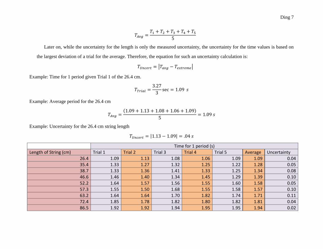
Ding 7

Later on, while the uncertainty for the length is only the measured uncertainty, the uncertainty for the time values is based on

the largest deviation of a trial for the average. Therefore, the equation for such an uncertainty calculation is:

| |

Example: Time for 1 period given Trial 1 of the 26.4 cm.

Example: Average period for the 26.4 cm

( )

Example: Uncertainty for the 26.4 cm string length

| |

Time for 1 period (s)

Length of String (cm) Trial 1 Trial 2 Trial 3 Trial 4 Trial 5 Average Uncertainty

26.4 1.09 1.13 1.08 1.06 1.09 1.09 0.04

35.4 1.33 1.27 1.32 1.25 1.22 1.28 0.05

38.7 1.33 1.36 1.41 1.33 1.25 1.34 0.08

46.6 1.46 1.40 1.34 1.45 1.29 1.39 0.10

52.2 1.64 1.57 1.56 1.55 1.60 1.58 0.05

57.3 1.55 1.50 1.68 1.55 1.58 1.57 0.10

63.2 1.64 1.64 1.70 1.82 1.74 1.71 0.11

72.4 1.85 1.78 1.82 1.80 1.82 1.81 0.04

86.5 1.92 1.92 1.94 1.95 1.95 1.94 0.02

Ding 8

Best Fit Line y = 0.2202x0.4903

R² = 0.9852

0.00

0.50

1.00

1.50

2.00

2.50

0.0 10.0 20.0 30.0 40.0 50.0 60.0 70.0 80.0 90.0 100.0

Tim

e f

or

1 P

eri

od

(s)

Length of String (cm ± 0.1 cm)

Effect of String Length on Period Time

Ding 9

Data Processing:

Before more information could be determined from the graph, we first need to linearize our

graph. After looking at the various regressions for the original data, it seemed clear that a power

fit, as , would be the best fit, meaning that

√

Therefore, to linearize the graph, we must take the square root of the length and plot that against

the time value, for a Time v √ graph. In order to do this, we simply calculated the square

root of each length, and proceeded to use that value as the new x value, as shown

through √ . Using the 26.4 cm as an example, the new x value would be √ , or

5.14. The new uncertainty rested on percent uncertainties, as well as special rules to follow when

linearizing items in this manner. Therefore, it is calculated by:

An example with 26.4 cm would be

A new data table is generated is following:

Ding 10

Linearized Data (cm^0.5) 1 Period (s)

Square Root Length Uncertainty Average Uncertainty 5.14 0.04 1.09 0.04

5.95 0.03 1.28 0.05 6.22 0.03 1.34 0.08

6.83 0.03 1.39 0.10

7.22 0.03 1.58 0.05 7.57 0.03 1.57 0.10

7.95 0.03 1.71 0.11 8.51 0.02 1.81 0.04

9.30 0.02 1.94 0.02

This generates the final graph, but we would also like to have maximum and minimum

slopes on it, so we shall calculate those points first, and then plot them.

The maximum slope is determined from the maximum uncertainty values of the highest

and lowest points, so that the two points responsible for this calculation would be: (

) and ( ). Using our data, these two

points would be (5.14 + 0.04, 1.09 -0.04) and (9.30 -0.02, 1.94 + 0.02), giving us the points

( ) ( )

The maximum slope is similarly calculated, but with all of the signs switched, giving the

points ( ) and ( ), or (5.14 - 0.04,

1.09 + 0.04) and (9.30 + 0.02, 1.94 - 0.02), and thus ( ) and ( ).

Ding 11

Note: Error bars in the x direction are on the graph, but the fact that they are extremely small, they do not show up well on the graph.

Best Fit Line y = 0.2069x + 0.0358

R² = 0.9844

Max Slope y = 0.2194x - 0.0839

Min Slope y = 0.1879x + 0.1687

0.00

0.50

1.00

1.50

2.00

2.50

0.00 2.00 4.00 6.00 8.00 10.00 12.00

Tim

e f

or

1 P

eri

od

(s)

Square Root of Length of String (cm^0.5)

Lineraized Effect of String Length on Period Time

Ding 12

Looking at our best fit line, several issues come up, some valuable while others are likely

to be mistakes. First, it is rather clear that there is a square root correlation between the length of

the string with the period of time, given factors such as the high correlation value, the best fit line

fitting cleanly between the max and min slope lines, and how the best fit line passes through

every region of uncertainty. However, other factors, such as the x and y intercepts, are likely due

to errors in the experiment. If we analyze the x-intercept, we would find that when the string is 0

cm long, the period would still be 0.0358 seconds. As this is a rather nonsensical answer, and

cannot be explained by simple air friction, it is likely that it is due to some other kind of error. In

addition, the y-intercept has a similar issue, as it implies that the only time when the period

would be 0 is when you have a negative string length.

Overall, our graph is sound in the way that it depicts the data, showing the relationship

varying with a very clear constant value.

Conclusion:

After the lab was finished, there was an effort to find reasoning in physics for the reason for the

square root correlation. In particular, I looked at various Simple Harmonic Motion calculations,

as well as the geometry of the pendulum, to determine some kind of coordinating equation.

To begin with, I recalled a basic equation that works with all oscillating objects: the equations

that deal with ω. Specifically, the equations

√

From this, the following is derived:

Ding 13

√

√

Using powers, we can simplify this to a better form:

( )

(

)

√

This seems somewhat close to our equation, as it does have a square root in it. What could we do

to eliminate the mass, as well as the k? For this, we turn to our force equations regarding SHM.

( )

( )

( )

After this, we must turn to a little bit of geometry.

As you can tell by the following diagram, it is possible to calculate the mathematical relationship

between the two.

From geometry, we know the following:

Ding 14

Substituting this into our previous equation for x, we get

( )

Due to our knowledge about calculus and the fact that the angle theta is relatively small, we can

evaluate that

( )

By the squeeze theorem, so that

Substituting this into our T equation, we get

√

√

And with a few more slight manipulations, we get

√ √

Ding 15

The physics explanation for this implies that changing the length of the string is inversely

correlated with changing the oscillation constant defined as . This reduces the angular

frequency, resulting in a larger period time.

One way to test how valid our data was is by comparing the derived equation with our

experimental equation. From our experiment, if we attribute the value to error, we have an

equation of √ . From our derived equation, we know that the constant should

equate to

√ . If we evaluate that, allowing g to be in

, we find that the constant should be

0.200606. This difference represents an error of only 2.90%, which means that this experiment

matches with the derived physics. In other words, this experiment can be slightly modified to

measure the gravitation constant at the location of the experiment. We can manipulate the

equation so that (

)

, so that when we plug in k, we can find the gravitational constant.

This method reveals that g would be 922

, which would be a percent error of 6.01%.

Some of the errors that may have resulted in such error include

variables such as an inaccurate measurement of drop height, but

primarily spin and pitch of the bob. Although it was not well explored, it

is possible that the variation in heights caused to some extent the error.

More likely, a clear problem was in how the pendulum swung. As it

moved through the air, I noticed how it often rotated along the axis perpendicular to the bob,

which may have resulted in the action robbing the object of some of its momentum, and thus

some of its energy. This would have caused the bob to have a slower stopping time than what

would have been expected.

Ding 16

Another one of the errors that I encountered is slightly harder to

image/draw, but is easily explainable. In our ideal pendulum, we would

have expected it to only move in one field of motion, such as in a two-

dimensional plane. However, in my experiment, the pendulum bob

moved in an ellipse pattern through 3-dimensional space. This may have

again resulted in complicated patterns attributed towards the three-

dimensional motion of an oscillating motion, while also removing from the actual nature of the

oscillations. For example, this motion viewed in two dimensions may appear to spend more time

around the edges/vertices than in the center, resulting in skewed data.

A random error was the way that the bob was timed. I attempted to time it as it

approached its maximum height, or the very slowest it would be. However, human eyes are not

particularly strong, and it is often quite difficult to judge the exact moment when the bob was at

its maximum. This is reflected through the uncertainty of the time data, which although is still

rather minimal, does reflect slight changes.

There are actually two simple methods that would fix quite a bit with this lab. The easiest

way would be to change the time at which I stopped the timer. Instead of timing the very top of

the curve, I should have instead timed it from the center of its swing. Both methods would have

resulted with the same data, but it would have been better and more accurate to measure the time

at a clearly defined point. Another, slightly more complex, method to fix this would be to limit

the pendulum to two dimensions of movement, through setting up barriers to prevent the bob

from swinging out too much. Although the restrictions themselves are prone to causing errors if

the bob bumps into them, the increased accuracy of path may result in a better experiment.

Finally, an even better measurement of the time would be to place a photo gate across the low

Ding 17

point of the pendulum, right in the center. Then, the photo gate would record each time the

pendulum passes through that point, giving a very accurate period. This would have been very

difficult to implement by itself, as you would have the issue of the bob accidentally hitting the

photo gate and knocking it off somehow, but if implemented together with the restricting to one

plane idea, it is likely that this would have greatly improved accuracy in our experiment.