Embed Size (px)
Citation preview

Master of Science Thesis
KTH School of Industrial Engineering and Management
Energy Technology EGI-2011-2012
Division of Innovative Sustainable Energy Engineering
SE-100 44 STOCKHOLM
Investigating CVT as a Transmission
System Option for Wind Turbines
Deniz Alkan

-2-
Master of Science Thesis EGI 2011:2012
Investigating CVT as a Transmission System
Option for Wind Turbines
Deniz Alkan
Approved
Examiner
Björn E. Palm
Supervisor
Nabil Kassem, Sad Jarall
Commissioner
Contact person
Abstract
In this study, an innovative solution is examined for transmission problems and frequency control for
wind Turbines. Power electronics and the gear boxes are the parts which are responsible of a significant
amount of failures and they are increasing the operation and maintenance cost of wind turbines.
Continuously transmission (CVT) systems are investigated as an alternative for conventional gear box
technologies for wind turbines in terms of frequency control and power production efficiency. Even
though, it has being used in the car industry and is proven to be efficient, there are very limited amount of
studies on the CVT implementation on wind turbines. Therefore, this study has also an assertion on being
a useful mechanical analyse on that topic. After observing several different types of possibly suitable CVT
systems for wind turbines; a blade element momentum code is written in order to calculate the torque,
rotational speed and power production values of a wind turbine by using aerodynamic blade properties.
Following to this, a dynamic model is created by using the values founded by the help of the blade
element momentum theory code, for the wind turbine drive train both including and excluding the CVT
system. Comparison of these two dynamic models is done, and possible advantages and disadvantages of
using CVT systems for wind turbines are highlighted. The wind speed values, which are simulated
according to measured wind speed data, are used in order to create the dynamic models, and Matlab is
chosen as the software environment for modelling and calculation processes. Promising results are taken
out of the simulations for both in terms of energy efficiency and frequency control. The wind turbine
model, which is using the CVT system, is observed to have slightly higher energy production and more
importantly, no need for power electronics for frequency control. As an outcome of this study, it is
possible to say that the CVT system is a candidate of being a research topic for future developments of
the wind turbine technology.
Key Words: Continuously variable transmission (CVT), wind turbine drive train, blade element
momentum (BEM), frequency control of wind turbines, power electronics.
-3-
Table of Contents
Abstract ........................................................................................................................................................................... 2
1 Introduction .......................................................................................................................................................... 6
1.1 Problem Definition ..................................................................................................................................... 7
2 State of Art ............................................................................................................................................................ 8
2.1 Variable Speed Theory ............................................................................................................................... 8
2.2 Power Electronics ....................................................................................................................................... 9
2.3 Wind Turbine Drive Trains .....................................................................................................................10
2.3.1 Direct Drive ......................................................................................................................................10
2.3.2 Geared Drive ....................................................................................................................................10
2.4 Continuously Variable Transmission .....................................................................................................11
2.4.1 CVT Types ........................................................................................................................................12
3 System Modelling ...............................................................................................................................................16
3.1 Torque Calculation ...................................................................................................................................17
3.2 Processing the Wind Speed Data ...........................................................................................................25
3.3 Dynamic Model of Wind Turbine Drive Train ....................................................................................29
3.4 Modelling the Drive train with CVT ......................................................................................................32
4 Results and Discussion ......................................................................................................................................34
4.1 Efficiency ....................................................................................................................................................40
4.2 CVT Dimensions ......................................................................................................................................42
5 Conclusion ...........................................................................................................................................................43
Bibliography .................................................................................................................................................................44
Appendix .......................................................................................................................................................................45

-4-
List of Figures
Figure 1 Power production of Variable Speed vs Fixed speed Wind Turbines .................................................. 8
Figure 2 Wind Turbine Power Electronics for Variable Speed Operation .......................................................... 9
Figure 3 Variable Diameter Pulley CVT system .....................................................................................................11
Figure 4 Automatically Regulated CVT ...................................................................................................................12
Figure 5 Basic Design Principle of HCVT .............................................................................................................13
Figure 6 Exploded view of CVT variator with core components .......................................................................14
Figure 7 Chain CVT ....................................................................................................................................................15
Figure 8 General view of the modelling processes flowchart ..............................................................................16
Figure 9 Critical Angles and Forces on Cross-section of a Blade .......................................................................18
Figure 10 Rotational Speed of the Rotor vs. Wind Speed ....................................................................................21
Figure 11 Aerodynamic Power vs. Wind Speed .....................................................................................................22
Figure 12 Power Coefficient vs. Wind Speed ........................................................................................................22
Figure 13 Varying Pitch Angles vs. Wind Speed ....................................................................................................23
Figure 14 Torque vs. Wind Speed ...........................................................................................................................24
Figure 15 Daily average wind speed for the best month ......................................................................................25
Figure 16 Daily average wind speed for the worst month ...................................................................................25
Figure 17 Hourly average wind speed for the best month ...................................................................................26
Figure 18 Hourly average wind speed for the worst month .................................................................................26
Figure 19 Simulated Wind Speed Data for the Worst Month Case ....................................................................27
Figure 20 Weibull distributions of measured and simulated data for worst month case .................................28
Figure 21 Weibull distributions of measured and simulated data for best month case ...................................28
Figure22 Layout of the wind turbine drive train ...................................................................................................29
Figure 23 The flowchart of the calculation .............................................................................................................31
Figure 24 Layout of the wind turbine drive train with CVT ................................................................................32
Figure 25 Power Production of the Turbine for the Worst Month Case ..........................................................34
Figure 26 Difference of Power Production of the Turbine with and without CVT ........................................35
Figure 27 Difference of Rotational Speed of the Turbine Rotor with and without CVT ...............................35
Figure 28 Rotational Speed of the Turbine Rotor for the Worst Month Case .................................................36
Figure 29 Variation of the CVT Ratio for the Worst Month Case .....................................................................37
Figure 30 Rotational Speed of the Generator input shaft for the Worst Month Case without CVT ............38
Figure 31 Rotational Speed of the Generator input shaft for the Worst Month Case with CVT..................38
Figure 32 Measured mechanical efficiency data of 30 mm GCI chain CVT .....................................................40
List of Tables
Table 1 Some of the CVT geared Passenger Vehicles...........................................................................................11
Table 2 Geometrical Properties of the Blades in Sections ...................................................................................17
Table 3 Varying torque values due to the varying wind speed values .................................................................29
Table 4 Mass moment of inertia values for turbine rotor and generator ...........................................................30
Table 5 Varying Turbine Parameters due to the Wind Speed with and without CVT ....................................33
Table 6 Energy Productions during Best and Worst Months with and without CVT ....................................34
Table 8 Efficiency values for different types of power converters .....................................................................41
Table 7 Typical Dimensions for Chain CVT System ............................................................................................42

-5-
Nomenclature
= Swept area of the blades
= Axial induction
= Tangential induction factor
= Critical axial induction factor
= Number of blades
= Drag coefficient
= Lift coefficient
= Normal force coefficient
= Power Coefficient
= Tangential force coefficient
= Drag Force
= Energy
= Prandtl’s Tip Loss Factor
= Gear ratio
= Total gear ratio with CVT
= Generator inertia
= Rotor inertia
= Lift force
= Power
= Normal component of force acting on blade
= Tangential component of force acting on
blade
= Rotor radius
= Local radius
= Torque
= Torque transmitted to CVT system
= Friction torque
= Generator torque
= Maximum rotor torque
= Rotor torque
= Time
= Wind speed
= Relative wind speed
= Rotational speed of the rotor
= Rotational speed of generator input shaft
= Rotational speed of wind turbine rotor
= Attack angle
= Twist angle
= Local pitch angle
= Pitch angle
= Inflow angle
= Density of air
= Tip speed ratio

-6-
1 Introduction
Energy is one of the essential needs of today’s society yet the energy production is a weighty problem.
Conventional energy production methods such as fossil fuel combustion are proven to be unsustainable
and environmentally unfriendly. Therefore, renewable energy sources are being used increasingly by the
time. Today, the wind energy technology is the fastest growing renewable energy technology, and it is a
common point of interest for the entire world.
In the year 2009, 273153 GWh of energy was produced by using wind power and this amount is
increasing every year while the wind energy production is becoming cheaper and more reliable (IEA,
2009). Many different designs and sizes of wind turbines are established already and new ones are being
established every other day, and they are proven to be useful. On the other hand, constructing and
designing them more cost competitive, more reliable and simpler are still issues. There are several serious
problems regarding wind turbines and frequency control is one of them. This study is written to
investigate an innovative transmission system option for wind turbines, which is called continuously
variable transmission (CVT), and has a potential to be a solution for this problem while increasing the
energy production rate of the turbine.
CVT technology is lately becoming a topic of interest among the wind energy researchers and wind
turbine produces, after it has been proven to be avail for the automotive industry in the past several
decades. It is a highlighted solution for the frequency control problem of wind turbines because of its
capacity of increasing the energy production efficiency, besides solving the problem in focus.
This study contains a detailed mechanical analyse of the effect of drive train systems on the energy
production of wind turbines. Instead of using the torque and rotational speed of the rotor values directly
taken from an existing wind turbine, these values are calculated by using BEM theory in order to keep
study open for further improvements due to the fact that the CVT system has a potential to increase wind
capture range of the turbine, which may need some additional developments on aerodynamic blade
properties; yet this improvements are remained as future work in order not to lose the focus of the study
and keep it in the area of drive train dynamics but not the aeroelastic or aerodynamic blade design.
Economical analyses and detailed strength calculations are not included to the frame of the study as well,
which are mainly depended on future improvements of CVT technology.
The comparison of two dynamic models is the methodology of this study, which of one includes the CVT
system besides the conventional gear box. The discussion of mechanical and electrical efficiency
differences and the effects of employing a CVT system in order to regulate the frequency, on rotational
speed and power production of the turbine can be found in this study. Besides, in order to do these
analyses, a rough investigation on today’s CVT technology and the possibility of future developments are
going to be observed and discussed.
-7-
1.1 Problem Definition
A wind turbine is a device, which transforms the kinetic energy of the wind into mechanical energy. Then,
this mechanical energy is converted into electrical energy in the generator. One of the main problems of
this conversion is the variable character of the wind speed. The generators have some constant range of
rotational speed, which is a fact that brings some limitations to the rotational speed of the wind turbine
rotor due to the stationary relationship between the speed of the wind turbine rotor and the generator
input shaft, which is caused by using constant gear ratios.
As a result of this constant gear ratio, the changes in the rotational speed of the wind turbine rotor results
with changes in the rotational speed of the generator input shaft which cause fluctuations at the frequency
of the generated electricity by the wind turbine, and this is a fact that decreases the electricity quality. In
order to increase the electricity quality and keep the frequency of electricity, which is sent to the grid,
constant, expensive power electronics are used in variable speed wind turbines, and this is another fact
which decreases the reliability and increases the cost of the wind energy.
Although the lifetime of a wind turbine is averagely estimated as 20 years, the lifetime of the gearbox is
generally much lower, estimated around 5 years (Ragheb & Ragheb, 2010). After this period, the gearbox
must be replaced, which is a fact that increases the operation and maintenance cost of wind turbines.
Changing the gearbox of a wind turbine can be as expensive as 10% of the construction cost of it (Ragheb
& Ragheb, 2010). This extra cost surely is decreasing the competition strength of wind turbines with other
power production methods. Therefore, the new trend for wind turbines is using direct drive and not to
use a gearbox, especially for the ones located in areas which are difficult to maintain such as offshore wind
turbines. On the other hand, direct drive systems are generally more expensive due to the necessity of the
high number of poles in the generator because of the low rotational speed in the generator input shaft.
Moreover, the weight and radius of the generators are increasing as well as their cost, while the number of
poles is increasing.
CVT technology is outstanding because of being a simple mechanical solution to en electrical problem.
Furthermore, possibility of increasing the energy production efficiency by using CVT technology is
making it worth to investigate. Even though, there is no wind turbine on use with CVT, there are some
promising researches shows the advantages of CVT implementation for wind turbines, and in the light of
these researches, it would not be unexpected to see wind turbines with CVT in a near future. In this
aspect, this study claims to be a contribution to the development of wind turbine technology.
.

-8-
2 State of Art
2.1 Variable Speed Theory
Wind energy is the term which is used for describing the kinetic energy of the wind flow. This kinetic
energy can be transformed into electrical energy by the help of wind turbines. Although the power density
of the wind is only related with the wind speed and the density of the air, the energy amount extracted
from the wind is also related with the wind turbine design. Power Coefficient (Cp) of a wind turbine is a
notation for the possible energy capture ratio from the wind flow through the blades. The theoretical Cp
of a wind turbine can be maximum 0.593, and this fact is known as Beltz’ law.
The maximum Cp values are reached while the wind turbine is operating at the optimum tip speed ratio
( ) so that the wind speed interval where the tip speed ratio is optimal is an important parameter in the
matter of the wind turbine efficiency. Constant rotational speed turbines can only achieve for a small
wind speed interval, and they are most efficient for these wind speeds. For variable speed wind turbines, w
is not constant; therefore the variable speed that wind turbines can operate in or close values of to
for a wider wind speed range. Hence, the aerodynamic efficiency of variable speed wind turbines is
higher. Especially for high wind speeds, the efficiency drop is not as dramatic as the constant variable
speed turbines for the variable speed ones, and they can produce the rated power for high wind speeds as
well, while the constant speed wind turbines can only produce the rated power for some certain wind
speed interval. One of the main aims of this study is to investigate the effects of the drive train on tip
speed ratio and the chance of further improvements.
Figure 1 Power production of Variable Speed vs. Fixed speed Wind Turbines (Santoso & Le, 2007)

-9-
2.2 Power Electronics
Because of the fact that variable gear sets are not employed in the wind turbines, the changes in the
rotational speed of the rotor, directly affect the rotational speed of the generator input shaft during
variable speed operation. This situation gives rise to the variable frequency problem. The frequency of the
grid is stable with a close range of variation at 50 Hz (60 Hz in USA), and when the frequency of the
generator varies more than some certain limit; circuit breakers cut the grid connection of the generator in
order to protect the grid. (Verdonschot, 2009)
The frequency of a generator is determined by the number of poles of the generator and the rotational
speed of the generator input shaft. The variable frequency problem can be solved by employing power
electronics between the generator and the grid. These power electronics are simply a rectifier that converts
the alternative current (AC), which has unstable frequency, to direct current (DC) and an inverter, which
converts DC to AC with stable frequency (see figure 1).
Figure 2 Wind Turbine Power Electronics for Variable Speed Operation (Verdonschot, 2009)
Even though, the power electronics technology is a relatively new technology, it is developing rapidly.
They are becoming widely available in the market, and the prices are decreasing. On the other hand, it is
possible to say that employing power electronics in the wind turbines is still expensive and decreases the
competition strength of wind power with conventional power generation techniques.
One other important disadvantage of power electronics is reliability. Power electronics are responsible of
25% of the total failures of wind turbines. Contrary to mechanical systems, failures are not predictable for
power electronics, which is a fact that increases the operation and maintenance cost of wind turbines.
Moreover, power electronics often fail due to the voltage spikes, and the cost of reparation is generally
relatively high. (Verdonschot, 2009)

-10-
2.3 Wind Turbine Drive Trains
Wind turbine drive trains consist of several components, which work together in a harmony. Roughly, a
drive train can be described as components of the wind turbine which carries the energy of the wind to
the generator in the form of torque and rotational speed. Several design alternatives of drive trains are
available in the wind turbine market nowadays, and newer drive train solutions are under investigation.
Although it is possible to classify drive trains in many ways, the classification chosen for this study is
according to their gear ratios and can be examined under the two titles below.
2.3.1 Direct Drive
In Direct drive systems, the gear ratio is equal to one, which means the rotor of the wind turbine is
directly coupled with the generator. The main advantage of these systems is that they eliminate the need of
a gearbox, and consequently decrease the operation and maintenance cost. Moreover, these systems are
more reliable and operate for a relatively longer time with fewer problems due to the reduced complexity.
On the other hand, because of the absence of the gearbox, the rotational speed of the generator input
shaft is equal to the rotor speed. In order to produce electricity at the desired frequency in low rotational
speeds; the pole number of the generators in direct drive systems is high. Hence, the generators used in
these systems are bigger, heavier and more expensive.
2.3.2 Geared Drive
The wind turbines, which use gear ratios bigger than 1, can be categorized under this title. A gearbox,
located between the rotor shaft and the generator shaft, is used for increasing the rotational speed of the
generator input shaft while decreasing the torque. By the help of the increased rotational speed of the
generator input shaft, the small number of poles is enough to obtain the desired frequency as the
generator output. Smaller and cheaper generators can be used in these systems. On the other hand,
because of the gearbox, the complexity of the system is higher than direct drive systems and these systems
are less reliable. Besides, due to the failure in the gearboxes, the operation and maintenance cost of these
systems are higher. The problems of these systems are forcing the producers to find alternative solutions.
Hybrid systems, which are a middle route between geared and direct drive systems, are one of the
solutions. The aim of hybrid systems is to decrease the complexity of the gearboxes and increase the
reliability without increasing the generator cost dramatically.
Moreover, producers are working on alternative gearbox and transmission system designs for wind
turbines, which can increase reliability and/or efficiency. The CVT system is one of these alternative
solutions. It is believed that CVT can improve efficiency of the wind turbines by increasing the wind
speed interval where the tip speed ratio is at its optimum value. Furthermore, it is believed that CVT use
can decrease the negative effects of fluctuations in the wind speed. CVT can keep rotational speed of
generator input shaft almost constant which would increase the electricity quality. (Cotrell, 2005)
Because of the possible advantages mentioned above, this study will investigate the CVT option as an
alternative transmission system solution for wind turbines.

-11-
2.4 Continuously Variable Transmission
CVT is simply a transmission system which allows the steeples gear ratio change between low and high
gear ratios (see figure 2). This property of the system provides an infinite number of speed and torque
ratios which makes the system attractive.
Figure 3 Variable Diameter Pulley CVT system (Motoress, 2011)
Although CVT is not a new technology, it became popular recently, especially for the automotive industry
(see Table 1). CVT provides improved fuel economy since with CVT system; it is possible to run the
vehicle at desired fuel consumption region independent from the velocity of it (Ryu & Kim, 2006).
Table 1 Some of the CVT geared Passenger Vehicles (Ragheb & Ragheb, 2010)
Producer Model Year
Honda Civic, High Torque 1995
Audi A4, A6 2000
Nissan Murano 2003
Ford Five Hundred, Freestyle 2005
Dodge Caliber 2007
Mitsubishi Lancer 2008
Nissan Maxima 2008
Honda Insight Hybrid 2010
With the increasing interest of the automotive industry on CVT systems, manufacturers started to develop
new types with the same principle. As a result of this, several different CVT types are available in the
market nowadays.

-12-
2.4.1 CVT Types
Although many types of CVT systems are available, only some of them might be suitable for wind turbine
applications. Torque capacity, reliability and scalability are some important factors to be considered to
decide which type of CVT system is the most suitable for wind turbines. This study has no intention of
making detailed analysis on every other CVT system, but it is a must to investigate some the most
approval ones.
2.4.1.1 Automatically Regulated CVT
Commonly, the variable diameter pulley CVT systems contain a spring acts on the driven pulley and
hydraulic or pneumatic system act on the driver pulley. Thus, the system can run at a given rotational
velocity independent from the torque transmitted. Automatically regulated CVT system is a variable
diameter pulley CVT system where both driven and driver pulleys are loaded with springs (see figure 3).
(Mangialardi & Mantriota, 1993)
Figure 4 Automatically Regulated CVT (Mangialard
& Mantriota, 1995)
Automatically regulated CVT is a highlighted
solution since it is an easy, cheap and reliable
system. In this system, the velocity ratios changes
due to the torque transmitted to the CVT from
the driver shaft. In the final analyse, it is possible
to say that, the torque and speed ratios between
driven and driver pulleys are depended variables
of the wind speed and these ratios are
continuously and automatically changing due to
changes in the wind speed. By using automatically
regulated CVT system, there is no need of control
equipment and hydraulic or pneumatic systems,
hence the CVT system is more reliable and more
cost efficient. (Mangialardi & Mantriota, 1993)
On the other hand, some problems such as
scalability and low torque capacity are still
standing. In order to decrease the amount of the
torque delivered to the system, an over gear is
necessary to be placed between wind turbine
rotor shaft and the driver shaft of the CVT
system. This over gear is not only increasing the
construction cost but also increasing the
operation and maintenance cost of the system.

-13-
2.4.1.2 Hoogenberg CVT (HCVT)
HCVT is a relatively new CVT technology which is developed for getting high efficiency at high torques. The working principle of HCVT is the ability of carrying over the torque and rotational speed from an infinitely long belt to a circular body while the belt is enclosed in it. For this system, the circular body is referred as carrier and the belt is referred as push belt (see Figure 4). In order to obtain the necessary friction force between the push belt and discs, a hydraulic clamping force is applied in this system. The transmission ratio, i, is changing according to changes in the positions of the push belt and the carrier with respected to the discs. In order to change the position of the carrier a swing arm is used in the system, which is a component of an electromechanical system. (Schouten, Filart, & Kouwenberg, 2006)
Figure 5 Basic Design Principle of HCVT (Schouten, Filart, & Kouwenberg, 2006)
Besides high torque capacity and high efficiency, scalability is another important advantage of the HCVT
system. While the diameter of the push belt is increasing, the torque capacity of the system is increasing
too. Moreover, it is possible to design the system for a sufficiently big interval of the coverage ratio.
(Schouten, Filart, & Kouwenberg, 2006)
On the other hand, the complexity of the system, the need of energy and a control system to keep it
running seems to be the disadvantages of the system. Additionally, there is no model available about wind
turbine applications of HCVT system yet, and this fact brings some reliability issues on the table.

-14-
2.4.1.3 Nu Vinci CVT
This system is a rolling traction transmission CVT system that uses the balls in order to vary the rotational
speed (see Figure 5). In this system power is transferred from the input disk to the put disk trough the
balls by using hydrodynamic lubrication. By changing the position of the idler on the longitudinal axis, it is
possible to change the rotational axis of the balls, which changes the transmission ratio (Cortell, 2004)
Figure 6 Exploded view of CVT variator with core components (Cortell, 2004)
One of the main advantages of the system is the ease of scalability. By increasing the number of the balls,
it is possible to increase the torque capacity of the system without any significant change in the efficiency
(Cortell, 2004). Moreover, this system is currently on use at the market for several industries although
there is no wind turbine that uses this system. Hence it is also possible to declare the system has a high
reliability.
One important drawback of this system is the need of energy and a control system to keep it running.
This is a fact that increases the complexity and the cost of the system, although the energy consumption is
not high and there is no need for a dramatically expensive control system.
-15-
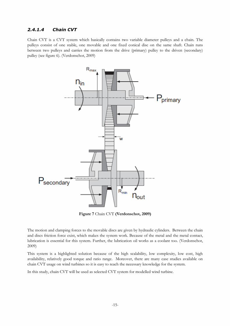
2.4.1.4 Chain CVT
Chain CVT is a CVT system which basically contains two variable diameter pulleys and a chain. The
pulleys consist of one stable, one movable and one fixed conical disc on the same shaft. Chain runs
between two pulleys and carries the motion from the drive (primary) pulley to the driven (secondary)
pulley (see figure 6). (Verdonschot, 2009)
Figure 7 Chain CVT (Verdonschot, 2009)
The motion and clamping forces to the movable discs are given by hydraulic cylinders. Between the chain
and discs friction force exist, which makes the system work. Because of the metal and the metal contact,
lubrication is essential for this system. Further, the lubrication oil works as a coolant too. (Verdonschot,
2009)
This system is a highlighted solution because of the high scalability, low complexity, low cost, high
availability, relatively good torque and ratio range. Moreover, there are many case studies available on
chain CVT usage on wind turbines so it is easy to reach the necessary knowledge for the system.
In this study, chain CVT will be used as selected CVT system for modelled wind turbine.

-16-
3 System Modelling
In order to model a wind turbine with the CVT system, first; an existing wind turbine is chosen and then
in order to calculate a realistic power production of this wind turbine; measured wind speeds are used in
this study. NTK 1500 is chosen as wind turbine, and the aerodynamic properties of the blades of this
turbine are used for calculations. Sprogø Island is chosen as location for wind speed data and the wind
speed data of this location is processed for calculations.
Figure 8 General view of the modelling processes flowchart
-17-
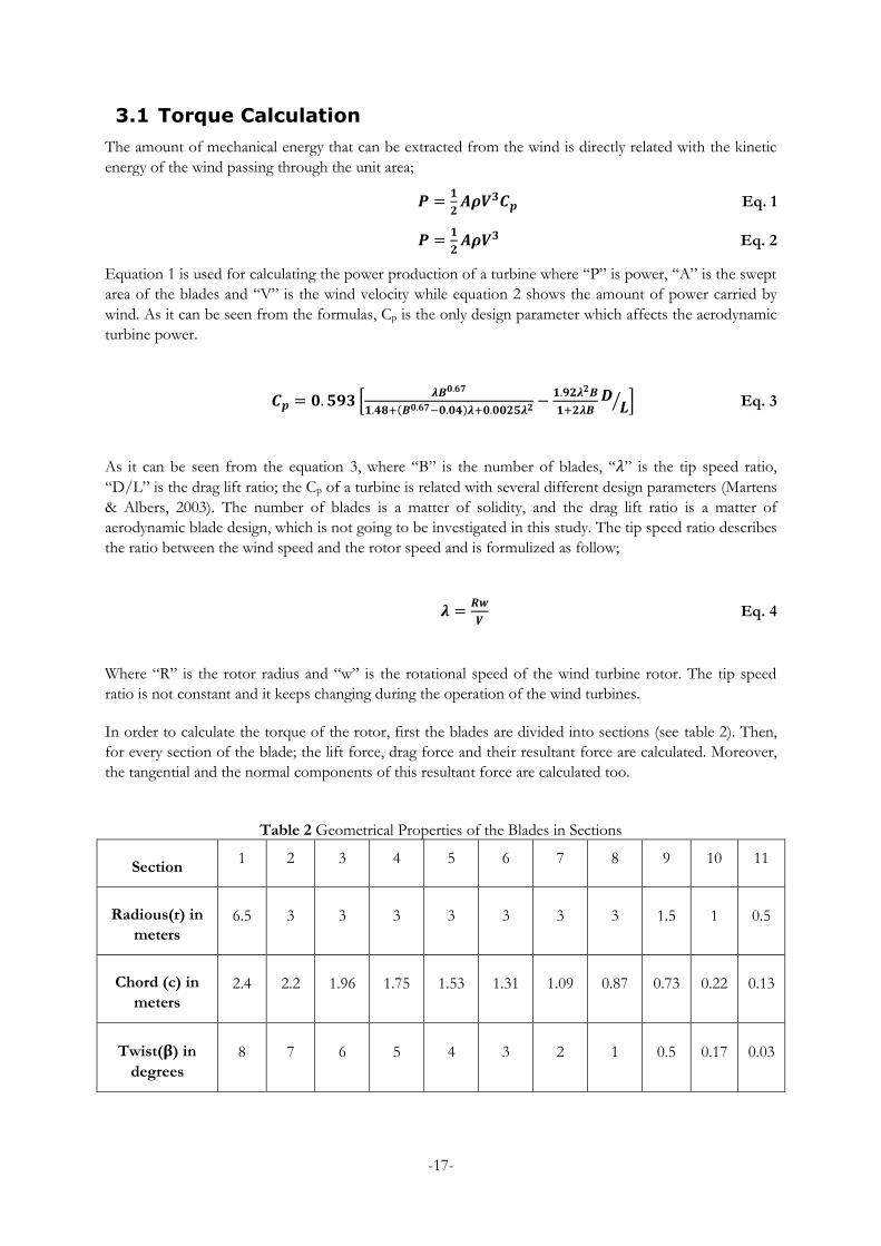
3.1 Torque Calculation
The amount of mechanical energy that can be extracted from the wind is directly related with the kinetic
energy of the wind passing through the unit area;
Eq. 1
Eq. 2
Equation 1 is used for calculating the power production of a turbine where “P” is power, “A” is the swept
area of the blades and “V” is the wind velocity while equation 2 shows the amount of power carried by
wind. As it can be seen from the formulas, Cp is the only design parameter which affects the aerodynamic
turbine power.
Eq. 3
As it can be seen from the equation 3, where “B” is the number of blades, “ ” is the tip speed ratio, “D/L” is the drag lift ratio; the Cp of a turbine is related with several different design parameters (Martens
& Albers, 2003). The number of blades is a matter of solidity, and the drag lift ratio is a matter of
aerodynamic blade design, which is not going to be investigated in this study. The tip speed ratio describes
the ratio between the wind speed and the rotor speed and is formulized as follow;
Eq. 4
Where “R” is the rotor radius and “w” is the rotational speed of the wind turbine rotor. The tip speed
ratio is not constant and it keeps changing during the operation of the wind turbines.
In order to calculate the torque of the rotor, first the blades are divided into sections (see table 2). Then,
for every section of the blade; the lift force, drag force and their resultant force are calculated. Moreover,
the tangential and the normal components of this resultant force are calculated too.
Table 2 Geometrical Properties of the Blades in Sections
Section 1 2 3 4 5 6 7 8 9 10 11
Radious(r) in
meters
6.5 3 3 3 3 3 3 3 1.5 1 0.5
Chord (c) in
meters
2.4 2.2 1.96 1.75 1.53 1.31 1.09 0.87 0.73 0.22 0.13
Twist( ) in
degrees
8 7 6 5 4 3 2 1 0.5 0.17 0.03

-18-
Figure 9 Critical Angles and Forces on Cross-section of a Blade (O.L.Hansen, 2008)
In order to do this, first, the axial and tangential induction factors are guessed as zero and an iteration
loop is written in Matlab to find their real values; for every section of the blade, for every other value of
wind speed and pitch angle. Moreover, in order to calculate these values, first the rotational speed of the
turbine ( ) is kept constant at the highest allowable value (due to the noise restrictions) of 2.35 rad/sec
and the radius of the turbine ( ) is accepted as 31 meters. After the initial guess of the axial and tangential
induction factors, the flow angle is calculated;
Eq. 5
Where; is the inflow angle, is the axial induction factor, is the tangential induction factor, is the
wind speed, which is varying between 5m/s to 25m/s, is the rotational speed and is rotor diameter
(O.L.Hansen, 2008). In order to find the lift and drag coefficients for the varying wind speeds and varying
pitch angles between -5 degrees to 30 degrees; the attack angle is calculated. For every other pitch angle
and wind speed, attack angles are found by using eq.2.2 and 2.3. By this procedure, a two dimensional
matrix the size of 21x35 is created with a different value of attack angle for every other wind speed and
pitch angle.
Eq. 6
Where; is the attack angle and is the local pitch angle which is a summation of the local twist of the
section and the pitch angle of the blade (O.L.Hansen, 2008). It can be calculated as follow;
Eq. 7
Where; is the pitch angle of the blade and is local twist angle of the blade (O.L.Hansen, 2008). By
using the turbine data sheet, the drag and lift coefficients, corresponding to the attack angle values are
found and interpolated, where it is necessary. After finding the drag and lift coefficients for the varying
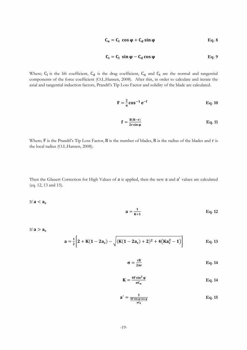
parameters, the coefficients of forces acting on the blades are calculated as follow;
-19-
Eq. 8
Eq. 9
Where; is the lift coefficient, is the drag coefficient, and are the normal and tangential
components of the force coefficient (O.L.Hansen, 2008). After this, in order to calculate and iterate the
axial and tangential induction factors, Prandtl’s Tip Loss Factor and solidity of the blade are calculated.
Eq. 10
Eq. 11
Where; is the Prandtl’s Tip Loss Factor, is the number of blades, is the radius of the blades and is
the local radius (O.L.Hansen, 2008).
Then the Glauert Correction for High Values of is applied, then the new and values are calculated
(eq. 12, 13 and 15).
If
Eq. 12
If
Eq. 13
Eq. 14
Eq. 14
Eq. 15
-20-
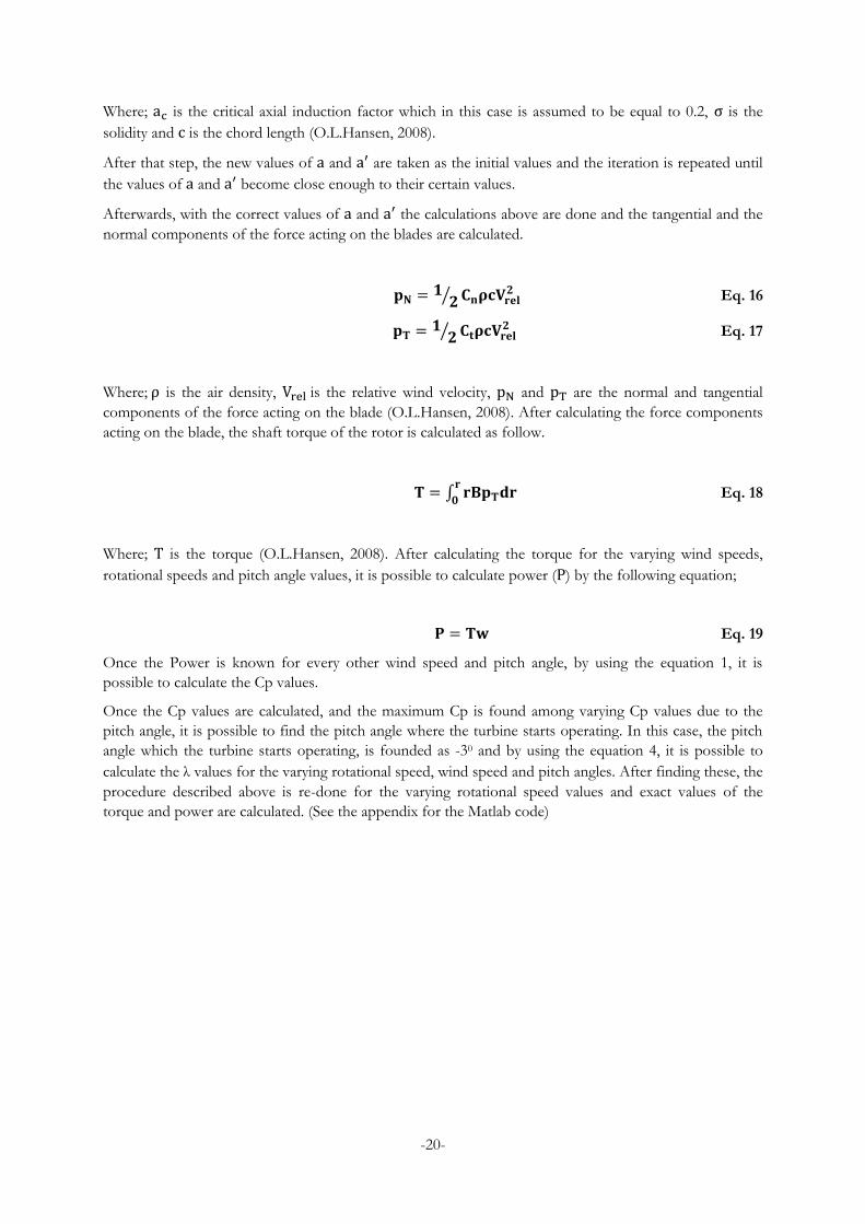
Where; is the critical axial induction factor which in this case is assumed to be equal to 0.2, is the
solidity and is the chord length (O.L.Hansen, 2008).
After that step, the new values of and are taken as the initial values and the iteration is repeated until
the values of and become close enough to their certain values.
Afterwards, with the correct values of and the calculations above are done and the tangential and the
normal components of the force acting on the blades are calculated.
Eq. 16
Eq. 17
Where; is the air density, is the relative wind velocity, and are the normal and tangential
components of the force acting on the blade (O.L.Hansen, 2008). After calculating the force components
acting on the blade, the shaft torque of the rotor is calculated as follow.
Eq. 18
Where; is the torque (O.L.Hansen, 2008). After calculating the torque for the varying wind speeds,
rotational speeds and pitch angle values, it is possible to calculate power ( ) by the following equation;
Eq. 19
Once the Power is known for every other wind speed and pitch angle, by using the equation 1, it is
possible to calculate the Cp values.
Once the Cp values are calculated, and the maximum Cp is found among varying Cp values due to the
pitch angle, it is possible to find the pitch angle where the turbine starts operating. In this case, the pitch
angle which the turbine starts operating, is founded as -30 and by using the equation 4, it is possible to
calculate the values for the varying rotational speed, wind speed and pitch angles. After finding these, the
procedure described above is re-done for the varying rotational speed values and exact values of the
torque and power are calculated. (See the appendix for the Matlab code)
-21-
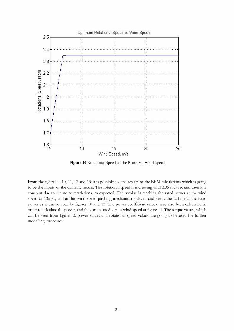
Figure 10 Rotational Speed of the Rotor vs. Wind Speed
From the figures 9, 10, 11, 12 and 13; it is possible see the results of the BEM calculations which is going
to be the inputs of the dynamic model. The rotational speed is increasing until 2.35 rad/sec and then it is
constant due to the noise restrictions, as expected. The turbine is reaching the rated power at the wind
speed of 13m/s, and at this wind speed pitching mechanism kicks in and keeps the turbine at the rated
power as it can be seen by figures 10 and 12. The power coefficient values have also been calculated in
order to calculate the power, and they are plotted versus wind speed at figure 11. The torque values, which
can be seen from figure 13, power values and rotational speed values, are going to be used for further
modelling_processes.

-22-
Figure 11 Aerodynamic Power vs. Wind Speed
Figure 12 Power Coefficient vs. Wind Speed

-23-
As mentioned before, the outcomes of this calculation are the torque, power and variable speed values of
the wind turbine which are changing due to the wind speed values between 5 to 25. 5 m/s is accepted as
the kick in wind speed for the wind turbine, and below this value the turbine is not working. Also as a
result of these calculations, it is possible to see how the power production of the wind turbine is changing
due to the rotational speed values. The important values of torque, rotational speed and power are the
ones for the wind speed interval from 5 to 7 m/s because of the fact that the rotational speed of turbine is
varying for this wind speed interval, and CVT mechanism has a difference from conventional gear box
systems while the rotor speed is not constant. These values can be found in table 3.
Table 3 Results of BEM code
Wind speed (m/s) Rotor Torque(kNm) Rotational Speed (rpm) Power (kW)
5 74.34 15.72 122.38
6 107.04 18.86 211.41
7 145.70 22.00 335.67
Figure 13 Varying Pitch Angles vs. Wind Speed

-24-
Figure 14 Torque vs. Wind Speed
The torque values, which can be seen at figure 13, have vital importance for further calculations also as
inputs of the dynamic models. The amount of the torque acting on the blades is increasing until the wind
speed reaches the value of 13 m/s and after this value; turbine reaches its rated power and the pitch
mechanism kicks in. Therefore, the torque value stays constant after this speed. Between the wind speeds
7 to 13, even thought the rotational speed of wind turbine is constant, the power value is increasing and
because of the fact that the torque acting on blades is increasing as it can be seen by the figures above.

-25-
3.2 Processing the Wind Speed Data
The wind speed data is the measured data from a 70 m mast at the island of Sprogø in the Great Belt
separating Fyn and Zealand. The measurements have been done for more than 20 years and the data are
10 minutes averages. Although the data is very detailed, it contains some noise. First, the noise is cleaned
by the help of a Matlab code. The second problem was the huge number of data points and in order to
have a more clear idea, the worst month and the best month in terms of wind speed is chosen as the
reference data among all these data. The daily and hourly wind speed characteristics of the worst and the
best months are plotted on graphs.
Figure 15 Daily average wind speed for the best month
Figure 16 Daily average wind speed for the worst month
-26-
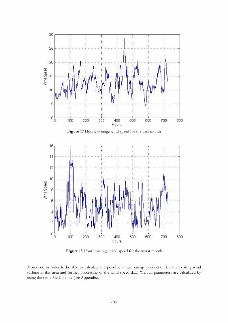
Figure 17 Hourly average wind speed for the best month
Figure 18 Hourly average wind speed for the worst month
Moreover, in order to be able to calculate the possible annual energy production by any existing wind
turbine in this area and further processing of the wind speed data, Weibull parameters are calculated by
using the same Matlab code (see Appendix).

-27-
The scale parameter is calculated as 9.2770 while the shape parameter is calculated as 2.2092. After
calculating these parameters, Weibull distribution and probability density function based on measured
wind data are found.
Once the Weibull distribution and the probability density function of the wind speed are found for the
measured data, a new set of data is created. The measured data was ten minutes averages, and for a
dynamic simulation, a wind speed datum is needed for every one second. Therefore, the new set of data is
created for every one second, by using the same standard deviation with the measured one. Moreover, the
ten minutes averages of the new set of data are equal to the measured data. In order to do this, rand
function of Matlab, which generates random numbers, is used with some restrictions (see Appendix for
the Matlab code).
Figure 19 Simulated Wind Speed Data for the Worst Month Case
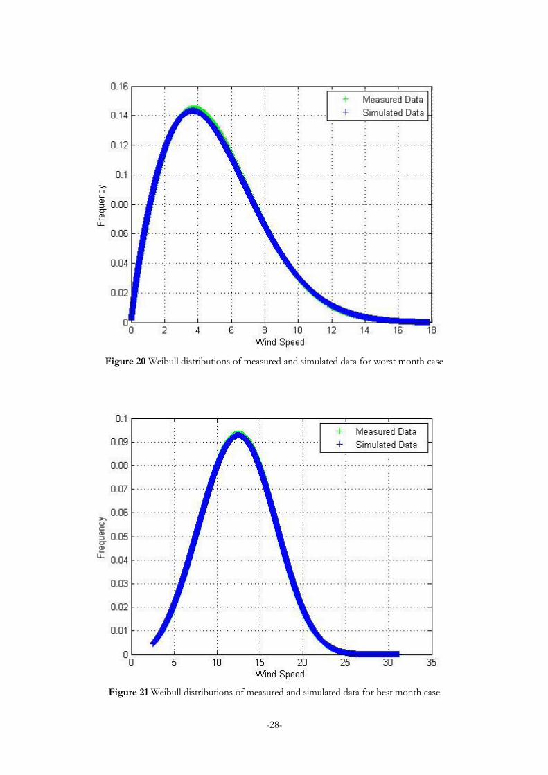
From figures 19 and 20 it is possible to see the Weibull distributions of the measured and simulated wind
speeds for both the worst and best month cases. From these figures, it can be seen that the simulated data
is close enough to the measured data to run the simulations on, even though they are not exactly the same
due to the factor of creating the simulated data randomly. The mean wind speed for simulated data for the
worst month case is 5.0427 m/s while the mean wind speed is 5.0354 m/s for the measured one. These
values are 12.4773 and 12.4771 m/s for the best month case, for simulated and measured data. For a
process which does not need very high precocity, these values can also be accepted as fairly close.
By considering that all, it is fair to state that the created data is realistic and suitable enough with the
measured one to be used as wind speed data, for further calculations and modelling.
-28-
Figure 20 Weibull distributions of measured and simulated data for worst month case
Figure 21 Weibull distributions of measured and simulated data for best month case
-29-
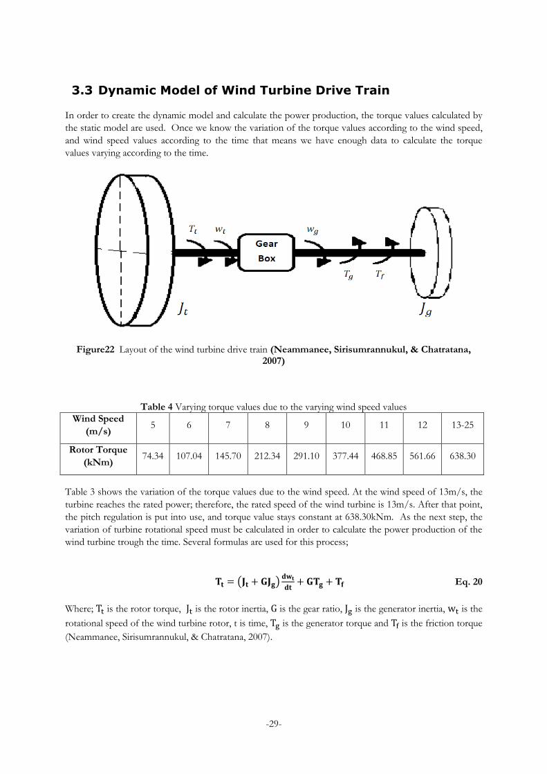
3.3 Dynamic Model of Wind Turbine Drive Train
In order to create the dynamic model and calculate the power production, the torque values calculated by
the static model are used. Once we know the variation of the torque values according to the wind speed,
and wind speed values according to the time that means we have enough data to calculate the torque
values varying according to the time.
Figure22 Layout of the wind turbine drive train (Neammanee, Sirisumrannukul, & Chatratana, 2007)
Table 4 Varying torque values due to the varying wind speed values
Wind Speed
(m/s) 5 6 7 8 9 10 11 12 13-25
Rotor Torque
(kNm) 74.34 107.04 145.70 212.34 291.10 377.44 468.85 561.66 638.30
Table 3 shows the variation of the torque values due to the wind speed. At the wind speed of 13m/s, the
turbine reaches the rated power; therefore, the rated speed of the wind turbine is 13m/s. After that point,
the pitch regulation is put into use, and torque value stays constant at 638.30kNm. As the next step, the
variation of turbine rotational speed must be calculated in order to calculate the power production of the
wind turbine trough the time. Several formulas are used for this process;
Eq. 20
Where; is the rotor torque, is the rotor inertia, is the gear ratio, is the generator inertia, is the
rotational speed of the wind turbine rotor, t is time, is the generator torque and is the friction torque
(Neammanee, Sirisumrannukul, & Chatratana, 2007).

-30-
As mentioned before, NTK 1500 is chosen for the rotor properties.
Table 5 Mass moment of inertia values for turbine rotor and generator (Wakileh, 2003)
Rotor (Jt) Generator(Jg)
Moment of Inertia (kgm2) 4.2x10⁶ 960
There is a direct relation existing between and the rotational speed of the generator input shaft ( ),
while the values of and are determining the power production. ;
Eq. 21
Eq. 22
For generator, a 1500 MW 6 poles VEM generator data are used. In order to keep the frequency of the
wind turbine at 50 Hz, a fix gear ratio of 1:45 is used for this 6 poles generator and that would result with
1010 rpm of the generator input shaft speed. The reason why the mechanical rotational speed of the
generator input shaft is chosen as 1010 rpm while the synchronous speed of the generator is 1000 rpm is;
while the speed of the generator input shaft is lower than the synchronous speed of the generator, the
generator works as a motor and takes energy from the grid instead of giving. (Verdonschot, 2009)
The difference between the mechanical rotational speed and the angular speed of the magnetic stator field
is known as “slip”. The slip percentage for the megawatt scale wind turbines is commonly around %1
(Hau, 2005). Therefore, a rotational speed of 1010 rpm is chosen in order to keep the slip percentage at
%1.
By using these three equations above (equation 20, 21 and 22), it is possible to create a dynamic
mathematical model of the wind turbine drive train (see appendix for Matlab code and flowcharts). Once
the variation of rotational speed and torque are calculated due to the time, it is possible to calculate the
amount of energy production.
Eq. 23
The friction losses, the gearbox and generator efficiencies are ignored during the calculation process
described above.
Also in order to solve the equation 20, the first value of mush be calculated. The generator and the
rotor are accepted as stationary for time (t) =0. While the generator is in the stationary position, the
generator torque ( ) is equal to zero since there is no power production. So the equation 20 can be
rewritten as;
Eq. 24
By accepting =0, it is possible to find the value of the as all the other values are known. Therefore
the flowchart of the calculation process which can be found in figure 22 is modified for the calculation of
initial value of by skipping the calculating the generator torque and using equation 24 instead of
equation 20 for the calculation of the rotor speed. At general flowchart (see figure 7), this step is marked
as 3.

-31-
Figure 23 The flowchart of the calculation
-32-
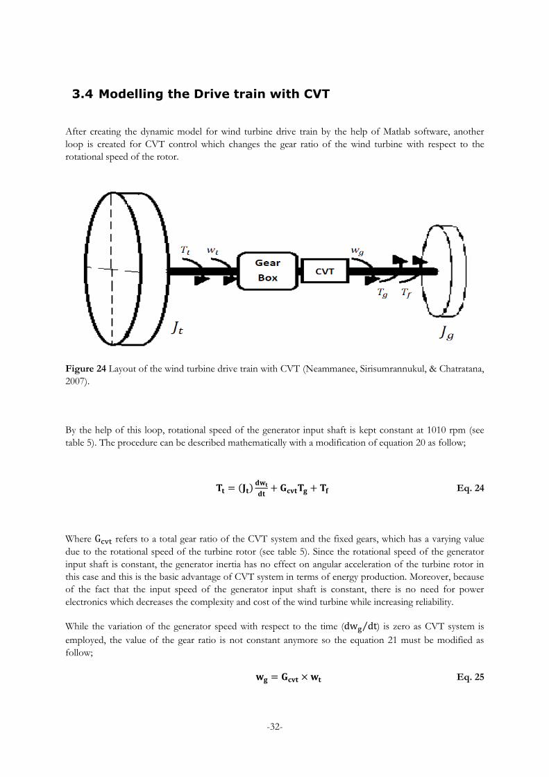
3.4 Modelling the Drive train with CVT
After creating the dynamic model for wind turbine drive train by the help of Matlab software, another
loop is created for CVT control which changes the gear ratio of the wind turbine with respect to the
rotational speed of the rotor.
Figure 24 Layout of the wind turbine drive train with CVT (Neammanee, Sirisumrannukul, & Chatratana,
2007).
By the help of this loop, rotational speed of the generator input shaft is kept constant at 1010 rpm (see
table 5). The procedure can be described mathematically with a modification of equation 20 as follow;
Eq. 24
Where refers to a total gear ratio of the CVT system and the fixed gears, which has a varying value
due to the rotational speed of the turbine rotor (see table 5). Since the rotational speed of the generator
input shaft is constant, the generator inertia has no effect on angular acceleration of the turbine rotor in
this case and this is the basic advantage of CVT system in terms of energy production. Moreover, because
of the fact that the input speed of the generator input shaft is constant, there is no need for power
electronics which decreases the complexity and cost of the wind turbine while increasing reliability.
While the variation of the generator speed with respect to the time ( ) is zero as CVT system is
employed, the value of the gear ratio is not constant anymore so the equation 21 must be modified as
follow;
Eq. 25

-33-
can mathematically be described as the multiplication of the fix gear ratio by the CVT ratio (see table
5). After that step by employing equations 22 and 23 again, it is possible to calculate the power and energy
production of the CVT implemented system.
Table 6 Varying Turbine Parameters due to the Wind Speed with and without CVT
Wind
Speed
(m/s)
Pitch Angle
(degrees)
Rotor
Speed
(rpm)
Fixed
Gear
Ratio
Generator
Speed
without CTV
(rpm)
CVT
Ratio
Generator
Speed with
CVT (rpm)
5 -3.00 15.72 1:45 707 1:1.43 1010
6 -3.00 18.86 1:45 848 1:1.19 1010
7 -3.00 22.00 1:45 990 1:1.02 1010
8 -3.00 22.44 1:45 1010 1:1 1010
9 -3.00 22.44 1:45 1010 1:1 1010
10 -3.00 22.44 1:45 1010 1:1 1010
11 -3.00 22.44 1:45 1010 1:1 1010
12 -3.00 22.44 1:45 1010 1:1 1010
13 -1.81 22.44 1:45 1010 1:1 1010
14 4.00 22.44 1:45 1010 1:1 1010
15 7.00 22.44 1:45 1010 1:1 1010
16 9.43 22.44 1:45 1010 1:1 1010
17 11.49 22.44 1:45 1010 1:1 1010
18 13.54 22.44 1:45 1010 1:1 1010
19 15.42 22.44 1:45 1010 1:1 1010
20 17.43 22.44 1:45 1010 1:1 1010
21 19.31 22.44 1:45 1010 1:1 1010
22 20.98 22.44 1:45 1010 1:1 1010
23 22.22 22.44 1:45 1010 1:1 1010
24 23.27 22.44 1:45 1010 1:1 1010
25 24.14 22.44 1:45 1010 1:1 1010

-34-
4 Results and Discussion
Because of the increased efficiency with CVT, the energy production performance of the turbine is
increasing. However; since the generator inertia is much smaller than the turbine inertia, this incensement
does not cause a significant change in the power production.
Table 7 Energy Productions during Best and Worst Months with and without CVT
Energy Production Without CVT
(MWh) With CVT
(MWh) Difference
(kWh)
Worst Month 153.9388 154.0257 86.8697
Best Month 809.7174 809.7317 14.3184
Figure 25 Power Production of the Turbine for the Worst Month Case
As it can be seen in table 6, the difference in the energy production is becoming much smaller for the
months which the wind speed is higher. The reason of this situation is; for the wind speeds higher than 7
m/s, the CVT system has no effect (see table 5) and in these months, the wind speed is hardly decreasing
below 7 m/s. For the months, which the wind speed is not that high, the CVT system causes a bit more
significant improvement on the performance of the wind turbine, on the other hand, these values are
calculated without considering the mechanical efficiency of the CVT system. When the mechanical
efficiency of CVT is taken into consideration, it is hard to say that. The CVT system is increasing the
energy production performance of the wind turbines with small generator inertia. While the inertia of the
generator is increasing relative to turbine rotor inertia, difference in the energy production is increasing
too. Moreover, the frequency control with the CVT system stands as a strong alternative to power
electronics, which is another important outcome of this study.

-35-
Figure 26 Difference of Power Production of the Turbine with and without CVT
Figure 27 Difference of Rotational Speed of the Turbine Rotor with and without CVT

-36-
In figure 25, it is possible to see the power production difference between two models. With the CVT
system, the turbine rotor has a higher value of acceleration due to the fact that the generator inertia is not
a parameter which increases the total inertia and decreases the angular acceleration. Therefore the turbine
rotor is reaching the optimum rotational speed, faster than the system, which does not contain CVT.
From figure 26, the difference can be seen between angular velocity variations during time between two
models. As expected, the turbine is accelerating faster when the CVT system is employed. Moreover the
difference between power productions, which is seen in figure 25, is smaller than the rotational speed
differences. This was another expected outcome due to the fact that the power production is not only
dependent on the rotational speed, but it is also dependent on the torque and the CVT system has no
effect on rotor torque, which is the main source of power. The CVT system is increasing the rotational
speed of the generator input shaft while it is decreasing the input torque; on the other hand, the
mechanical power transmitted is not changing, by neglecting the mechanical efficiencies. As a result of this
the only difference between the two systems in terms of power production is caused by the difference
between the angular acceleration, but still the effect of generator inertia is relatively small on angular
acceleration, which is the reason why the difference of the power production between the two systems are
not significant. On the other hand, for the wind turbines with higher generator inertias these differences in
both power production and rotational speed would be more significant.
Figure 28 Rotational Speed of the Turbine Rotor for the Worst Month Case

-37-
Figure 29 Variation of the CVT Ratio for the Worst Month Case
While it is possible to see variations of the CVT ratio during the worst month, it is possible to see the
effect of the CVT system on the rotational speed of the generator input shaft by comparing figures 29 and
30. As expected, with the help of the CVT system, the speed of the generator input shaft is remaining
constant. This situation gives rise to a 0.056% of energy production efficiency increase for the worst
month case, which is described and showed above (see table 6). As mentioned before, this efficiency
increase is caused by the total inertia drop due to the fact that the generator inertia is not decreasing the
angular acceleration of the generator input shaft; hence the generator speed is constant. The efficiency
would incense higher for the turbines which are using generators with higher inertia. As an example, when
the simulations run by multiplying the generator inertia by 10, the efficiency difference between the two
systems becomes 0.32% instead of 0.056%. On the other hand, turbines with higher generator inertia are
using direct drive option and there is no CVT system available on the market which can handle high
torque loads of direct drive wind turbines, currently.
Moreover, as it can be seen in figure 30, the CVT system is providing a constant generator speed, which
eliminates the need for power electronics as expected as well, while the rotational speed of the generator
input shaft is varying for the system which does not use the CVT, as it can be seen from figure 29. The
frequency of the electricity produced is constant when the CVT is implemented, and this outcome is the
main difference between the two systems, hence the energy production performance is not significantly
higher with CVT.
-38-
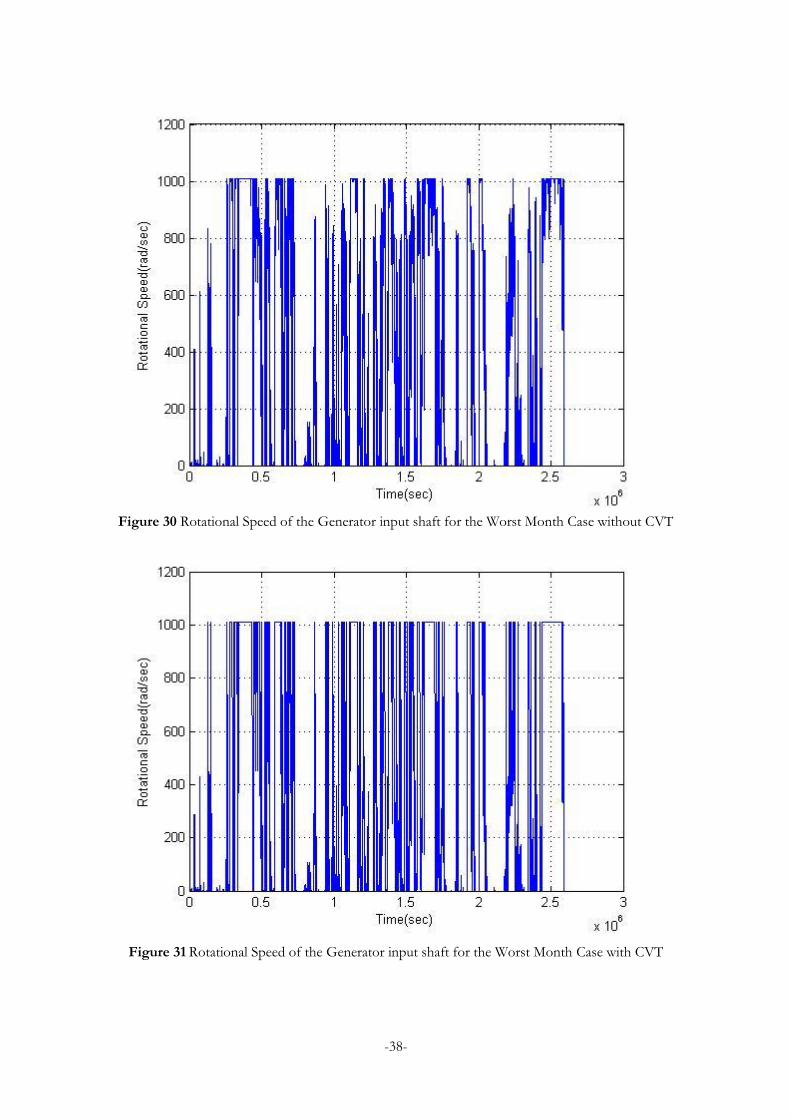
Figure 30 Rotational Speed of the Generator input shaft for the Worst Month Case without CVT
Figure 31 Rotational Speed of the Generator input shaft for the Worst Month Case with CVT

-39-
Furthermore by comparing the figures 29 and 30 in terms of difference between the rotational input shafts
speeds of the generator further commends can be done. While the system which uses CVT is achieving
the rated speed for a wider wind speed range, naturally for a wider time interval, the system which does
not use CVT is failing to do the same. This is the main difference between two systems, which gives rise
to some possible future improvements. By employing CVT systems, it is possible to produce energy while
the wind speed is lower, which means CVT system can decrease the kick in wind speed of wind turbines.
Therefore, one other important fact that increases energy performance of CVT implemented systems is
the wider operation range. CVT system can let a wind turbine start operating in lower wind speeds and by
doing this the energy production during the time, especially for the terms which the wind speed is not
high, would increase for the wind turbine. On the other hand, in order to make a fair comparison between
CVT including and excluding systems, the operation range of both models are taken same. Therefore it is
possible to say, CVT system would lead more energy production incensement than it has been calculated
in this study even though the value of produced energy would not be significantly higher than this because
of the fact that the wind energy is proportional with the third power of wind speed, which means the
amount of energy produced in low wind speeds a relatively small amount.
Moreover, in terms of frequency control CVT seems to be a very promising, mechanical alternative to
power electronics. As it can be seen by figure 30 and mentioned before, the generator input shaft speed is
almost constant for the system which uses CVT; therefore there is no need for power electronics to
control the frequency of produced electricity.
-40-
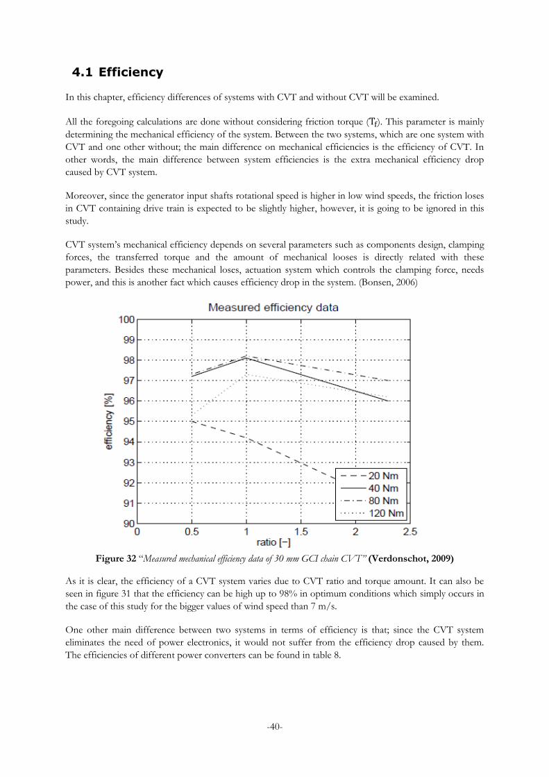
4.1 Efficiency
In this chapter, efficiency differences of systems with CVT and without CVT will be examined.
All the foregoing calculations are done without considering friction torque ( ). This parameter is mainly
determining the mechanical efficiency of the system. Between the two systems, which are one system with
CVT and one other without; the main difference on mechanical efficiencies is the efficiency of CVT. In
other words, the main difference between system efficiencies is the extra mechanical efficiency drop
caused by CVT system.
Moreover, since the generator input shafts rotational speed is higher in low wind speeds, the friction loses
in CVT containing drive train is expected to be slightly higher, however, it is going to be ignored in this
study.
CVT system’s mechanical efficiency depends on several parameters such as components design, clamping
forces, the transferred torque and the amount of mechanical looses is directly related with these
parameters. Besides these mechanical loses, actuation system which controls the clamping force, needs
power, and this is another fact which causes efficiency drop in the system. (Bonsen, 2006)
Figure 32 “Measured mechanical efficiency data of 30 mm GCI chain CVT” (Verdonschot, 2009)
As it is clear, the efficiency of a CVT system varies due to CVT ratio and torque amount. It can also be
seen in figure 31 that the efficiency can be high up to 98% in optimum conditions which simply occurs in
the case of this study for the bigger values of wind speed than 7 m/s.
One other main difference between two systems in terms of efficiency is that; since the CVT system
eliminates the need of power electronics, it would not suffer from the efficiency drop caused by them.
The efficiencies of different power converters can be found in table 8.

-41-
Table 8 Electrical efficiency values for different types of power converters (Marckx, 2006)
Wind Speed (m/s) SiC MOSFETs/SiC
Schottkys, 3 kHz
SiC MOSFETs/SiC
Schottkys, 9kHz
SiC MOSFETs/SiC
Schottkys, 50 kHz
5 94.3% 93.8% 90.7%
5.5 95.5% 95.1% 92.2%
6 96.3% 95.9% 93.2%
6.5 96.9% 96.5% 93.9%
7 97.3% 97.2% 94.4%
7.5 97.5% 97.3% 94.8%
8 97.7% 97.4% 95.0%
8.5 97.8% 97.4% 95.2%
9 97.8% 97.4% 95.3%
9.5 97.7% 97.4% 95.3%
10 97.7% 97.3% 95.3%
10.5 97.6% 97.1% 95.3%
11 97.4% 97.0% 95.1%
11.5 97.3% 97.0% 95.0%
12 97.3% 97.0% 95.0%
12.5 97.3% 97.0% 95.0%
13 97.3% 97.0% 95.0%
13.5 97.3% 97.0% 95.0%
14 97.3% 97.0% 95.0%
14.5 97.3% 97.0% 95.0%
25 97.3% 97.0% 95.0%
All in all, while CVT system causes mechanical efficiency drop and consumes power, it prevents electrical
efficiency drop caused by power electronics. Since there are no detailed efficiency data available for a CVT
system which is suitable for wind turbine in the case of this study, it is not possible to make a detailed
analysis of overall efficiency difference between integrating and not integrating the CVT system for this
case. On the other hand, by observing the data available, it can be said that the total efficiency drop caused
by employing a CVT mechanism in wind turbine would not cause a significantly lower efficiency than
employing power electronics.
-42-
4.2 CVT Dimensions
One other important discussion point about CVT systems is the possibility and feasibility of producing
CVT systems for high torque applications such as wind turbines. It is clear that producing drive train parts
for wind turbines, which are subjected to high and varying torques for years of operation, is a relatively
though area (Fairley, 2009). Therefore, it is necessary to make detailed fatigue and strength analyses,
besides scaling investigations for large scaled CVT systems for wind turbines, which is not done in this
study.
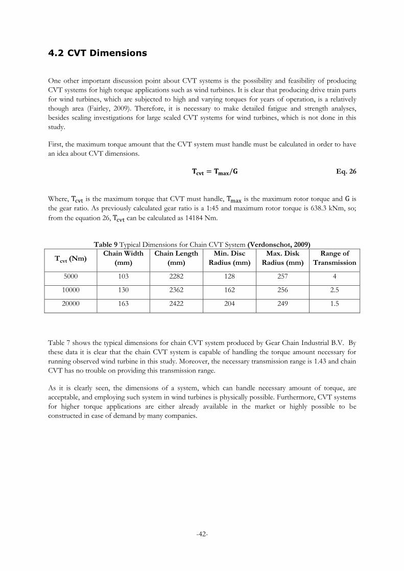
First, the maximum torque amount that the CVT system must handle must be calculated in order to have
an idea about CVT dimensions.
Eq. 26
Where, is the maximum torque that CVT must handle, is the maximum rotor torque and is
the gear ratio. As previously calculated gear ratio is a 1:45 and maximum rotor torque is 638.3 kNm, so;
from the equation 26, can be calculated as 14184 Nm.
Table 9 Typical Dimensions for Chain CVT System (Verdonschot, 2009)
Tcvt (Nm) Chain Width
(mm)
Chain Length
(mm)
Min. Disc
Radius (mm)
Max. Disk
Radius (mm)
Range of
Transmission
5000 103 2282 128 257 4
10000 130 2362 162 256 2.5
20000 163 2422 204 249 1.5
Table 7 shows the typical dimensions for chain CVT system produced by Gear Chain Industrial B.V. By
these data it is clear that the chain CVT system is capable of handling the torque amount necessary for
running observed wind turbine in this study. Moreover, the necessary transmission range is 1.43 and chain
CVT has no trouble on providing this transmission range.
As it is clearly seen, the dimensions of a system, which can handle necessary amount of torque, are
acceptable, and employing such system in wind turbines is physically possible. Furthermore, CVT systems
for higher torque applications are either already available in the market or highly possible to be
constructed in case of demand by many companies.

-43-
5 Conclusion
First of all, it is possible to increase power production performance of wind turbines by employing CVT
mechanism as it can be seen trough this study, even though it is an insignificant difference. The generator
inertia is the key factor which determines the incensement of performance, in other words, while the
generator inertias is getting bigger, the difference between CVT integrated system and the commercial
system is increasing in terms of power production performance. Therefore, CVT system integration can
be also examined for direct drive systems which have much bigger generators and direct proportionally to
this, much bigger generator inertias. One other discussion is naturally reliability in this case. The aim of
using the direct drive technology for wind turbines is decreasing the operation and maintenance cost, also
by eliminating the risk of gearbox failures, increasing the reliability. Considering this fact, the CVT system
may not seem like the first choice, on the other hand, by using CVT system it is possible not to use power
electronics, which decreases the risk of failure. In this manner, before suggesting a solution, more
researches must be done related the reliability of CVT system on wind turbines but with primary analyses
it can be claimed that CVT system is a promising as an alternative frequency control solution. Also,
eliminating the usage of power electronics can provide some cost reduction depend on CVT cost.
Some problems that can be formed by CVT integration such as lubrication and overheating have not been
mentioned and observed during this study but they clearly need to be discussed.
One other possible advantage of CVT can be the operation range of wind turbine. By employing CVT
system it is possible to control the speed of generator input shaft which means the wind turbines with
CVT can have smaller kick in wind speeds and rotor speeds. The generator’s working speed interval
would not be a troubling detail, which limits the operation range of wind turbine, by the help of variable
speed ratios provided by CVT.
Furthermore, CVT system can also change the generator trends of wind turbines since it is much less
problematic to use a synchronous generator when a CVT system is mechanically controlling the input
speed. This fact can decrease the complexity of synchronous generator use, by eliminating the need of
complex control systems, which is the main reason that the induction generators are more often used in
wind turbine applications. Even though this is another noteworthy discussion topic, this study has not
observed generator types and selection.
The aim of this study was examining CVT system as a transmission system solution by creating a
mechanical model of drive train with CVT and observing the power production performance
improvements and it is fulfilled. CVT system seems to be a good and promising method to increase the
energy efficiency of wind turbines on study.
As future work, various tasks can be accomplished. A complete strength calculation is necessary to figure
out the reliability of CVT systems. Further, the possible incensement in power production due to the
widened operation wind speed interval is another topic to observe in order to understand the pros and
cons of CVT implementation in wind turbines. The torque calculation for this study is done by using
BEM code, so that; it is possible to do these observations by small changes in the code for every other
wind turbine which has known aerodynamic properties. Finally, the economical assessment and life time
analyses are also crucial to be done before having a final judgment about CVT as a transmission system
option for wind turbines.
-44-
Bibliography
Bonsen, B. (2006). Efficiency optimization of the pushbelt CVT by variator slip control. Eindhoven:
Eindhoven University of Technology.
Cortell, J. (2004). Motion Technologies CRADA CRD-03-130: Assessing the Potential of a Mechanical Continuously
Variable Transmission. Golden: National Renewable Energy Laboratory.
Cotrell, J. (2005). Assessing the Potential of a Mechanical Continuously Variable Transmission for Wind
Turbines. Windpower 2005. Denver: National Renewable Energy Laboratory.
Fairley, P. (2009, October 29). Testing Cheap Wind Power. Technology Review .
Hau, E. (2005). Wind Turbines: Fundamentals, Technologies, Application, Economics. Springer.
IEA. (2009). Renewables and Waste in World in 2009. http://www.iea.org: International Energy Agency.
Mangialard, L., & Mantriota, G. (1995). Dynamic Behaviour of Wind Power Systems Equipped with
Automatically Regulated Continuously Variable Transmission. Renewable Energy , 185-203.
Mangialardi, L., & Mantriota, G. (1993). Automatically Regulated C.V.T. in Wind Power Systems.
Renewable Energy , 299-310.
Marckx, D. (2006). Breakthrough in Power Electronics from SiC. Wilsonville: National Renewable Energy
Laboratory.
Martens, A., & Albers, P. (2003). Investigation into CVT application in Wind Turbines. Eindhoven.
Motoress. (2011). Scooter's Stepless Acceleration Secret is in the CVT. http://www.motoress.com.
Neammanee, B., Sirisumrannukul, S., & Chatratana, S. (2007). Development of a Wind Turbine Simulator.
International Energy Journal , 21-28.
O.L.Hansen, M. (2008). Aerodynamics of Wind Turbines. Copenhagen.
Ragheb, A., & Ragheb, M. (2010). Wind Turbine Gearbox Technologies. 1st International Nuclear and
Renewable Energy Conferance. Amman.
Ryu, W., & Kim, H. (2006). Belt-pulley mechanical loss for a metal belt continuously variable
transmission. Journal of Automative Engineering , 57-65.
Santoso, S., & Le, H. T. (2007). Fundamental time–domain windturbine models for windpower studies.
Renewable Energy , 2436–2452.
Schouten, M., Filart, B., & Kouwenberg, J. (2006). HCVT - A new high torque CVT system integrating.
Eindhoven.
Verdonschot, M. (2009). Modeling and Control of wind turbines using a Continuously Variable Transmission.
Eindhoven: Eindhoven University of Technology.
Wakileh, G. J. (2003). GE 1.5 MW, 60 Hz Wind Turbine General Data. Tehachapi: GE Wind Energy.

-45-
Appendix
Matlab Codes
1. BEM Code
1.1 Main Code
close all clear all clc
%%Inputs and Preparation of Arrays and Matrices%%
w=22.44*pi/30;%rotational speed in radian per seconds (assumed value) ro=1.225;%density of air in kilogram per cubic meters R=62/2;%radius in meters load airfoil.dat ;%loading the airfoil data (Cl and Cd values for
corresponding angle of attack) B=input('number of blades: '); %command window input for number of blades rad=[6.5;9.5;12.5;15.5;18.5;21.5;24.5;27.5;29;30;30.4]; %strips in meters b=[8;7;6;5;4;3;2;1;0.5;0.17;0.03]; % twist in degrees c=[2.4;2.2;1.96;1.75;1.53;1.31;1.09;0.87;0.73;0.22;0.13]; %chord length in
meters V=5:25;%wind speed in meters per second ptc=-6:3:30;%pitch angles in degrees Size=size(ptc);%finding numbers of pitch angles S=Size(1,2); %finding numbers of pitch angles L=zeros(S,3);% creating L martix P=zeros(21,1);%creating P(power) array Cp=zeros(21,1);% creating Power coefficient(Cp) array lambda=zeros(21,1);%creating lambda(tip speed ratio) array Table_Thrust=zeros(21,S);%creating Table_Thrust(Thrust Force) matric Table_CT=zeros(21,S);%creating Table_CT(Thrust Coefficiant) matric Table_P=zeros(21,S);%creating Table_P(Power) matrix Table_Cp=zeros(21,S);%creating Table_P(Power) matrix Table_lambda=zeros(21,S);%creating Table_lambda(tip speed ratio) matrix data=zeros(11,7);%creating data matrix %% %%Calculations for Constant Rotational Speed%%
for m=1:S % m is the caunter for picth angels pitch=ptc(1,m); for k=1:21 %k is the caunter for wind speeds Vo=V(1,k); for i=1:11% i is the caunter for strips,chord length and twist r=rad(i,1); chord=c(i,1); beta=b(i,1);
[a,a1,Vrel,Pt,Pn,CT,T]=function1(beta,chord,r,B,airfoil,Vo,pitch,w);%sendin
g inputs and geting outputs from function data(i,1)=r; %filling the function outputs to data matrix data(i,2)=a; data(i,3)=a1; data(i,4)=Pt; data(i,5)=Pn; data(i,6)=CT;

-46-
data(i,7)=T; end%end of i loop sum=0;%creating sum intager for i=1:10% i is the caunter for integration int=0.5*(data(i+1,1)*data(i+1,4)+data(i,1)*data(i,4))*(data(i+1,1)-
data(i,1)); sum=sum+int;%sum is the result of integration end%end of i loop P(k,1)=B*w*sum;%calculating power values for varying wind speeds Cp(k,1)=P(k,1)/(0.5*ro*(Vo^3)*pi*R^2);%calculating Cp values for varying
wind speeds lambda(k,1)=w*R/Vo;%calculating tip speed ratio values for varying wind
speed end%end of k loop L(m,1)=pitch;%first column of L matrix is pitch angles L(m,2)=max(Cp);%second column of L matrix is maximum Cp values for varying
pitch angles X=Cp(:,1)==max(Cp);%X is an array to chose maximum Cp values L(m,3)=lambda(X,1);%third column of L matrix is tip speed ratios
corresponding maximum Cp values end%end of m loop Cp_max=max(L(:,2));%Cp_max is the maximum Cp value disp(Cp_max)%maximum Cp output x=L(:,2)==max(L(:,2));%x is an array to chose values corresponding to
Cp_max pitch_opt=L(x,1);%pitch_opt is optimum pitch angle disp(pitch_opt)%optimum pitch angle output lambda_opt=L(x,3);%lambd_opt is optimum tip speed ratio disp(lambda_opt)%optimum tip speed ratio output
%%
%%Calculations for Rotational Speed%%
W=zeros(21,S);%creating W matrix for m=1:S%m is the caunter acording to varying pitch angles for i=1:21%i is the caunter acording to varying wind speeds W(i,m)=(L(m,3)*V(1,i))/R;%calculating rotational speeds if W(i,m)<=2.35%conditionally chosing rotational speed values W(i,m)=W(i,m);%numbers smaller than 2.35 are not changing else W(i,m)=2.35;%numbers bigger than 2.35 are becoming 2.35 end%end of if condition end%end of i loop end%end of m loop figure; plot(V,W(:,x))%ploting the wind speed versus rotational speed
corresponding to the lamda_opt title('Optimum Rotational Speed vs Wind Speed') xlabel('Wind Speed') ylabel('Rotational Speed') grid on %%
%%Calculations for Varying Rotational Speed%%
for m=1:S%m is the caunter for picth angels pitch=ptc(1,m); for k=1:21%k is the caunter for wind speeds and rotational speeds Vo=V(1,k);

-47-
w=W(k,m); for i=1:11% i is the caunter for strips,chord length and twist r=rad(i,1); chord=c(i,1); beta=b(i,1);
[a,a1,Vrel,Pt,Pn,CT,T]=function1(beta,chord,r,B,airfoil,Vo,pitch,w);%sendin
g inputs and geting outputs from function data(i,1)=r;%filling the function outputs to data matrix data(i,2)=a; data(i,3)=a1; data(i,4)=Pt; data(i,5)=Pn; data(i,6)=CT; data(i,7)=T; end%end of i loop T_r=0;%creating T_r intager sum=0;%creating sum intager for i=1:10% i is the caunter for integration int=0.5*(data(i+1,1)*data(i+1,4)+data(i,1)*data(i,4))*(data(i+1,1)-
data(i,1)); sum=sum+int;%integration for power Thr=((data(i,7)+data(i+1,7))*0.5)*(data(i+1,1)-data(i,1)); T_r=T_r+Thr;%integration for thrust end%end of i loop Table_P(k,m)=B*W(k,m)*sum;%Table_P matrix is filled with power values
varying due to pitch, rotational speed and wind speed Table_Cp(k,m)=Table_P(k,m)/(0.5*ro*(Vo^3)*pi*R^2);%Table_Cp matrix is
filled with Cp values Table_lambda(k,m)=W(k,m)*R/Vo;%Table_lambda matrix is filled with tip speed
ratio values Table_Thrust(k,m)=T_r;%Table_Thrust matrix is filled with thrust values
varying due to pitch, rotational speed and wind speed Table_CT(k,m)=Table_Thrust(k,m)/(0.5*ro*Vo^2*pi*R^2); end%end of k loop end%end of m loop %% %%Calculations for Cp Values Due to the Varying Wind Speeds%%
P_regul=1500000;%rated power value in watts Cp_T=zeros(21,1);%creating Cp_T array Cp_N=zeros(21,1);%creating Cp_N array for i=1:21%i is the counter for Cp values Cp_T(i,1)=2*P_regul/((V(1,i)^3)*ro*pi*R^2);%Cp_T array is the Cp values
necesarry for rated power if max(Table_P(i,:))<=P_regul%if the available power smaller than the rated
power for a spesific wind speed Cp_N(i,1)=Table_Cp(i,x);%then Cp_N array is filled by Cp values for
optimum pitch angle elseif max(Table_P(i,:))>P_regul%if the available power bigger than the
rated power for a spesific wind speed Cp_N(i,1)=Cp_T(i,1);%then Cp_N array is filled by Cp values necesarry
to limit the power at rated power end%end of if condition end%end of i loop j=1;%creating j integer(to use as a caunter) Vc=5;%creating Vc integer(to use as critical wind speed) while Cp_N(j,1)==Table_Cp(j,x)%condition is Cp values in Cp_N must be equal
to Cp values at optimum pitch angle Vc=Vc+1;%if the condition is obtained, Vc value will increase by one j=j+1;%if the condition is obtained, j value will increase by one

-48-
end%end of condition disp(Vc)%critical Wind Speed output %% %%Calculations for Power, Thrust and Pitching%%
Pitching=zeros(21,1);%creating Pitching array Pitching(:,1)=pitch_opt;%Pitching array is filled by optimum pitch angle
value CT_N=zeros(21,1);%creating CT_N array CT_N(:,1)=Table_CT(:,x);% T_Force array is filled by Trust values for
optimum pitch angle for j=j:21%j is the caunter and the first value of j is due to critical
Wind Speed(see between 147-152) for k=2:S%k is the caunter and the last value of k is due to number of
pitch angles if Table_Cp(j,k)>Cp_N(j,1)&&Table_Cp(j,k-1)<=Cp_N(j,1) %in this condition loop, first the intervals of pith angles, necesarry for
Cp values are found Pitching(j,1)=ptc(1,k)-((Table_Cp(j,k)-Cp_N(j,1))*(ptc(1,k)-ptc(1,k-
1)))/(Table_Cp(j,k)-Table_Cp(j,k-1)); CT_N(j,1)=Table_CT(j,k)-((Table_Cp(j,k)-Cp_N(j,1))*(Table_CT(j,k)-
Table_CT(j,k-1)))/(Table_Cp(j,k)-Table_Cp(j,k-1)); %then the pitch angels and Thrust Coefficiant values are interpolated due
to Cp values. elseif Table_Cp(j,k-1)>Cp_N(j,1)&&Table_Cp(j,k)<=Cp_N(j,1) Pitching(j,1)=ptc(1,k-1)-((Table_Cp(j,k-1)-Cp_N(j,1))*(ptc(1,k-1)-
ptc(1,k)))/(Table_Cp(j,k-1)-Table_Cp(j,k)); CT_N(j,1)=Table_CT(j,k-1)-((Table_Cp(j,k-1)-Cp_N(j,1))*(Table_CT(j,k-1)-
Table_CT(j,k)))/(Table_Cp(j,k-1)-Table_Cp(j,k)); end%end of condition end%end of k loop end%end of j loop P_N=zeros(21,1);%creating P_N array T_Force=zeros(21,1);%creating T_Force array for i=1:21%i is counter for power and thrust coefficiant P_N(i,1)=0.5*Cp_N(i,1)*(V(1,i))^3*ro*pi*R^2/1000;%calculating the power due
to the wind speed in kilowatts T_Force(i,1)=(0.5*CT_N(i,1)*ro*V(1,i)^2*pi*R^2);%calculating the thrust
coefficiant due to the wind speed end%end of i loop figure; plot(V,Pitching)%plotting pitch angels versus wind speed title('Pitch Angle vs Wind Speed') xlabel('Wind Speed') ylabel('Pitch Angle') grid on figure; plot(V,P_N)%plotting power versus wind speed title('Power vs Wind Speed') xlabel('Wind Speed') ylabel('Power') grid on figure; plot(V,Cp_N)%ploting power coefficiant versus wind speed title('Cp vs Wind Speed') xlabel('Wind Speed') ylabel('Cp') grid on figure; plot(V,T_Force)%plotting thrust versus wind speed title('Thrust vs Wind Speed')
-49-
xlabel('Wind Speed') ylabel('Thrust') grid on figure; plot(V,CT_N)%plotting thrust coefficiant versus wind speed title('Thrust Coefficiant vs Wind Speed') xlabel('Wind Speed') ylabel('Thrust Coefficiant') grid on %%
%%Calculations for Annual Energy Production%%
WB=wblpdf(V,9.277,2.209);%weibull function of wind speed AEO=0;%creating AEO intager for i=1:20%i is the counter for integration int=(0.5*(P_N(i,1)+P_N(i+1,1)))*WB(1,i); AEO=AEO+int; end%end of i loop AEP=AEO*365*24;%result of integration times hours in a year disp(AEP)%Annual energy production output
1.2 Function
function
[a,a1,Vrel,Pt,Pn,CT,T]=function1(beta,chord,r,B,airfoil,Vo,pitch,w)
ro=1.225;%density of air in kilogram per cubic meters a=0;%axial induction factor a1=0;%tangential induction factor R=62/2;%radius in meters ac=0.2;%critical axial induction factor for j=1:20%j is the counter for iteration fi=atand((1-a)/((1+a1)*(r*w/Vo)));%calculating flow angle in degrees teta=beta+pitch;%calculating the local pitch angle in degrees alfa=fi-teta;%calculating the angle of attack in degrees for i=1:32%i is the counter for drag and lift coefficients
interpolation if alfa>airfoil(i,1) && alfa<airfoil(i+1,1)%interpolation due to
condition Cl=airfoil(i,2)-((airfoil(i,2)-airfoil(i+1,2))*(alfa-
airfoil(i,1)))/(airfoil(i+1,1)-airfoil(i,1)); Cd=airfoil(i,3)-((airfoil(i,3)-airfoil(i+1,3))*(alfa-
airfoil(i,1)))/(airfoil(i+1,1)-airfoil(i,1)); elseif alfa<airfoil(i,1) && alfa>airfoil(i+1,1) Cl=airfoil(i,2)-((airfoil(i,2)-airfoil(i+1,2))*(alfa-
airfoil(i,1)))/(airfoil(i+1,1)-airfoil(i,1)); Cd=airfoil(i,3)-((airfoil(i,3)-airfoil(i+1,3))*(alfa-
airfoil(i,1)))/(airfoil(i+1,1)-airfoil(i,1)); elseif alfa==airfoil(i,1) Cl=airfoil(i,2); Cd=airfoil(i,3); end%end of condition end%end of i loop Cn=Cl*cosd(fi)+Cd*sind(fi);%calculating Cn Ct=Cl*sind(fi)-Cd*cosd(fi);%calculating Ct

-50-
F=(2/pi)*acos((exp(-B/2*(R-r)/(r*sind(fi)))));%calculating Prandtl's
tip loss factor sigma=chord*B/(2*pi*r);%calculating solidity K=(4*F*sind(fi)*sind(fi))/(sigma*Cn);%calculating K if a<=ac%condition for Glauert correlation a=1/(((4*F*sind(fi)*sind(fi))/(sigma*Cn))+1);%recalculating a for a<0.2 CT=4*a*(1-a)*F;%calculating thrust coefficient for a<0.2 elseif a>ac a=0.5*(2+K*(1-2*ac)-sqrt((K*(1-2*ac)+2)^2+4*(K*ac*ac-1))); %recalculating a for a>0.2 CT=4*(ac*ac+(1-2*ac)*a)*F;%calculating thrust coefficient for a>0.2 end%and of condition a1=1/(((4*F*sind(fi)*cosd(fi))/(sigma*Ct))-1);%recalculating a' Vrel=(1-a)*Vo/sind(fi);%calculating relative wind speed Pt=0.5*ro*Vrel^2*chord*Ct;%calculating tangential component of p Pn=0.5*ro*Vrel^2*chord*Cn;%calculating normal component of p T=CT*0.5*ro*Vo*2*pi*R;%calculating the thrust end%end of j loop

-51-
2. Dynamic modelling and wind speed processing
clear all close all clc load sprog.tsv; ratio=1/45; T=[74.3352;107.0427;145.6970;212.3358;291.0965;377.4432;468.8507;561.6586;6
38.2979;638.2979;638.2979;638.2979;638.2979;638.2979;638.2979;638.2979;638.
2979;638.2979;638.2979;638.2979;638.2979]*1000; w=[1.6456;1.9747;2.3038;2.3500;2.3500;2.3500;2.3500;2.3500;2.3500;2.3500;2.
3500;2.3500;2.3500;2.3500;2.3500;2.3500;2.3500;2.3500;2.3500;2.3500;2.3500]
; CVT_ratio=105.75./w; Pow=zeros(10,3); Pow(2:10,1)=T(1:9).*w(1:9); Pow(2:10,2)=T(1:9); Pow(2:5,3)=w(1:4); Pow(6:10,3)=[2.36;2.37;2.38;2.39;2.4]; I_r=4.2*10^6; I_g=960; I=I_r+I_g/ratio; I_cvt=I_r+I_g*31.5; %%cleaning the noise from data x=sprog(:,2)>=90; sprog(x,:)=[]; sprog; y=sprog(:,3)>360 & sprog(:,4)>360; sprog(y,:)=[]; sprog; dist=sprog(:,3); A=size(dist); a=A(1,1);
ha=zeros(183517,1); k=1; da=zeros(7646,1); ma=zeros(254,1); for i=1:6:183517*6 ha(k,1)=mean(sprog(i:i+6,2));%mean hourly wind speed data k=k+1; end k=1; for i=1:24:7646*24 da(k,1)=mean(ha(i:i+24,1));%mean daily wind speed data k=k+1; end k=1; for i=1:30:254*30 ma(k,1)=mean(da(i:i+30,1));%mean monthly wind speed data k=k+1; end [r]=find(ma(:,1)==max(ma)); [s]=find(ma(:,1)==min(ma)); plot(da((r-1)*30+1:r*30+1)) xlabel('Days') ylabel('Wind Speed') grid on figure; plot(da((s-1)*30+1:s*30+1)) xlabel('Days')

-52-
ylabel('Wind Speed') grid on figure; plot(ha((r-1)*720+1:r*720+1)) xlabel('Hours') ylabel('Wind Speed') grid on figure; plot(ha((s-1)*720+1:s*720+1)) xlabel('Hours') ylabel('Wind Speed') grid on figure; Vmax=(sprog((r-1)*720*6+1:r*720*6+1,2)); Vmin=(sprog((s-1)*720*6+1:s*720*6+1,2)); for i=1:length(Vmax) if Vmin(i,1)<1 Vsmin((i-1)*600+1:i*600,1)=Vmin(i,1)+Vmin(i,1).*rand(600,1); else Vsmin((i-1)*600+1:i*600,1)=Vmin(i,1)-1+2.*rand(600,1); end Vsmax((i-1)*600+1:i*600,1)=Vmax(i,1)-1+2.*rand(600,1); end plot(Vsmin) xlabel('Seconds') ylabel('Wind Speed') grid on B=zeros(a,1); for i=1:a if sprog(i,3)>360 B(i,1)=sprog(i,4); elseif sprog(i,4)>360 B(i,1)=sprog(i,3); else B(i,1)=(sprog(i,3)+sprog(i,4))/2; end end
%% creating the new matrix with one direction data
F=zeros(a,3); F(:,1)=sprog(:,1); F(:,2)=sprog(:,2); F(:,3)=B(:,1); W=F(:,2); Mean=mean(W); Std=std(W); Y=normpdf(W,Mean,Std); plot(W,Y,'r+') xlabel('Wind Speed') ylabel('Frequency') hold on
%%creating the figure %%Creation of the histogramme
[H,x]=hist(F(:,2),33); H=H/a; %%create the figure bar(x,H) %%put the next graph on the same figure

-53-
%deleting the zero wind speed values from the array for weibull dist.% z=F(:,2)==0; F(z,:)=[];
%%Weibull A and K and Plot Wd=wblfit(F(:,2)); A=Wd(1); k=Wd(2); %%calculate the weitbull fonction with the A and K Weibull(:,1)=wblpdf(F(:,2),A,k); %%plot on the same figure the weilbull function plot(F(:,2),Weibull(:,1),'g+'); hold off xlabel('Wind Speed') ylabel('Frequency') %% M=zeros(40,3); M(:,1)=0:39; M(6:26,2)=T; M(6:26,3)=w; T_r=zeros(length(Vsmin),1); W=zeros(length(Vsmin),1); tor=zeros(length(Vsmin),2); w_r=zeros(length(Vsmin),1); for s=1:length(Vsmin) T_r(s,1)=interp1(M(:,1),M(:,2),Vsmin(s,1)); w_r(s,1)=interp1(M(:,1),M(:,3),Vsmin(s,1)); if W(s,1)<2.35 tor(s,1)=interp1(Pow(:,3),Pow(:,2),W(s,1)); else pow=T_r(s,1)*W(s,1);%%% tor(s,1)=interp1(Pow(:,1),Pow(:,2),pow);%% end a=(T_r(s,1)-tor(s,1))/I;% if W(s,1)+a<w_r(s,1) W(s+1,1)=W(s,1)+a; else W(s+1,1)=w_r(s,1); end % if W(s,1)<=w_r(s,1) % if a+W(s,1)<w_r(s,1) % W(s+1,1)=W(s,1)+a; % else % W(s+1,1)=w_r(s,1); % end % else % if Vsmin(s,1)>25 % W(s+1,1)=0; % else % W(s+1,1)=W(s,1)-(tor(s,1)/I); % if W(s+1,1)<0 % W(s+1,1)=0; % end % end % end end W_cvt=zeros(length(Vsmin),1); for s=1:length(Vsmin) % x=round(Vsmin(s,1))==M(:,1);
-54-
% T_r(s,1)=M(x,2);
if W_cvt(s,1)<w(1,1) tor(s,2)=interp1(Pow(:,3),Pow(:,2),W_cvt(s,1)); a=(T_r(s,1)-tor(s,1))/I_cvt;% elseif W_cvt(s,1)>w(1,1) && W_cvt(s,1)<2.35 tor(s,2)=interp1(Pow(:,3),Pow(:,2),W_cvt(s,1)); a=(T_r(s,1)-tor(s,1))/I_r; else pow=T_r(s,1)*W_cvt(s,1);%%% tor(s,2)=interp1(Pow(:,1),Pow(:,2),pow);%% a=(T_r(s,1)-tor(s,1))/I_r; end
if W_cvt(s,1)+a<w_r(s,1) W_cvt(s+1,1)=W_cvt(s,1)+a; else W_cvt(s+1,1)=w_r(s,1); end
% w_r=M(x,3); % if W_cvt(s,1)<w(1,1) % a=(T_r(s,1)-tor(s,2))/I_cvt;% % else % a=(T_r(s,1)-tor(s,2))/I_r;% % end % if W_cvt(s,1)<=w_r(s,1) % if a+W_cvt(s,1)<w_r(s,1) % W_cvt(s+1,1)=W_cvt(s,1)+a; % else % W_cvt(s+1,1)=w_r(s,1); % end % else % if Vsmin(s,1)>25 % W_cvt(s+1,1)=0; % else % W_cvt(s+1,1)=W_cvt(s,1)-(tor(s,2)/I); % if W_cvt(s+1,1)<0 % W_cvt(s+1,1)=0; % end % end % end end E=0; E_cvt=0; for s=1:size(T_r)-1 s1=(W(s)*tor(s,1)+W(s+1)*tor(s+1,1))/2/3600000;%kWh s2=(W_cvt(s)*tor(s,2)+W_cvt(s+1)*tor(s+1,2))/2/3600000;%kWh E=E+s1; E_cvt=E_cvt+s2; end figure; plot(W(1:2592600).*tor(:,1)/1000) xlabel('Time(sec)') ylabel('Power(kW)') grid on hold on plot(W_cvt(1:2592600).*tor(:,2)/1000,'r') E_dif=E_cvt-E%kWh x=(W_cvt*CVT_ratio(1,1)*60/2/pi)<1000; Wg_cvt=ones(length(Vsmin),1)*45*w(12,1)*60/pi/2;

-55-
Wg_cvt(x,1)=W_cvt(x,1)*31.5*60/2/pi; Wg(:,1)=W(:,1)*45*60/2/pi; figure; plot(Wg) xlabel('Time(sec)') ylabel('Rotational Speed(rad/sec)') grid on figure; plot(Wg_cvt) xlabel('Time(sec)') ylabel('Rotational Speed(rad/sec)') grid on figure; CVT=Wg_cvt(:,1)*(2*pi/60)/45./W_cvt(:,1); plot(CVT) xlabel('Time(sec)') ylabel('CVT Ratio') grid on