Inversion of Z-Axis Tipper Electromagnetic (Z-TEM) Data

The UBCThe UBCGeophysical Inversion FacilityGeophysical Inversion Facility

Elliot Holtham and Douglas Oldenburg

Outline

Introduction

Transfer functions and Z-TEM data

Conducting block example

Synthetic inversion

Field data inversion

Conclusions

Questions / Discussion

Z-TEM Technique

Z-TEM technique uses natural source fields similar to the magnetotelluric (MT) technique

Vertical magnetic fields due to natural sources are recorded over the survey area

Z-TEM Technique

Data relates the vertical magnetic field to the horizontal field at some fixed grounded reference station

Reference station compensates for unknown source field amplitude

Large areas can be surveyed quickly and economically

Promising technique to find large scale structures at depth

Transfer Functions

Transfer functions relate the vertical magnetic field measured above the earth to the horizontal magnetic field at some fixed reference station

Two unknowns and only one equation

Source polarization is assumed to be random

Use measurements from independent source polarizations

Computation of Transfer Functions for a Conducting Block

Source electric field into the page

Resulting charge buildup leads to a secondary current

Conducting block

Transfer Function Computation for Synthetic Example

Secondary electric fieldResulting transfer functions

Inversion of Z-TEM Data

Inversion algorithm has been implemented

2)( re fm mmW

)(][,)][(2

Q umdmW d fFF o b sd where

: Regularization parameterQ: Projection matrix u: Fields : Observed data : Model and Reference model

o b sd

re fmm ,

Wd, W : Data error, model weighting

Minimize = d + m

Inversion of Z-TEM Data

Minimize = d + m

)()( mgmWWJJ δTT Gauss-Newton method

)(]][[)( re fTo b sT

dT F mmWWdmWJmg

m

Synthetic Inversion Example

•Data computed at 1, 3.2, 5.6, 10, 18, 32 Hz

•Reference Station: (-3000, -3000, 0)m

•Data collected at a constant height of 100m

•Data collected over an area of 2500 x 2500m

•10m data spacing and 50m line spacing

Synthetic Inversion1 Hz

Observed data

Predicted data

Misfits

Synthetic Inversion3.2 Hz

Misfits

Observed data

Predicted data

Synthetic Inversion5.6 Hz

Misfits

Observed data

Predicted data

Synthetic Inversion10 Hz

Misfits

Observed data

Predicted data

Synthetic Inversion18 Hz

Misfits

Observed data

Predicted data

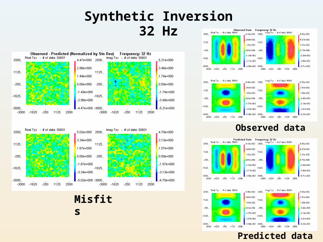
Synthetic Inversion32 Hz

Misfits

Observed data

Predicted data

Misfit

Target misfit: 1.2E+06Final misfit: 1.39E+06

Misfit

Synthetic Inversion ModelDepth 0 m

True Model Inverted Model

Synthetic Inversion ModelDepth -500 m

True Model Inverted Model

Synthetic Inversion ModelDepth -1000 m

True Model Inverted Model

Synthetic Inversion ModelDepth -1500 m

True Model Inverted Model

Synthetic Inversion ModelDepth -3000 m

True Model Inverted Model

Synthetic Inversion ModelNorthing -1500 m

True Model Inverted Model

Synthetic Inversion ModelNorthing -500 m

True Model Inverted Model

Synthetic Inversion ModelNorthing 0 m

True Model Inverted Model

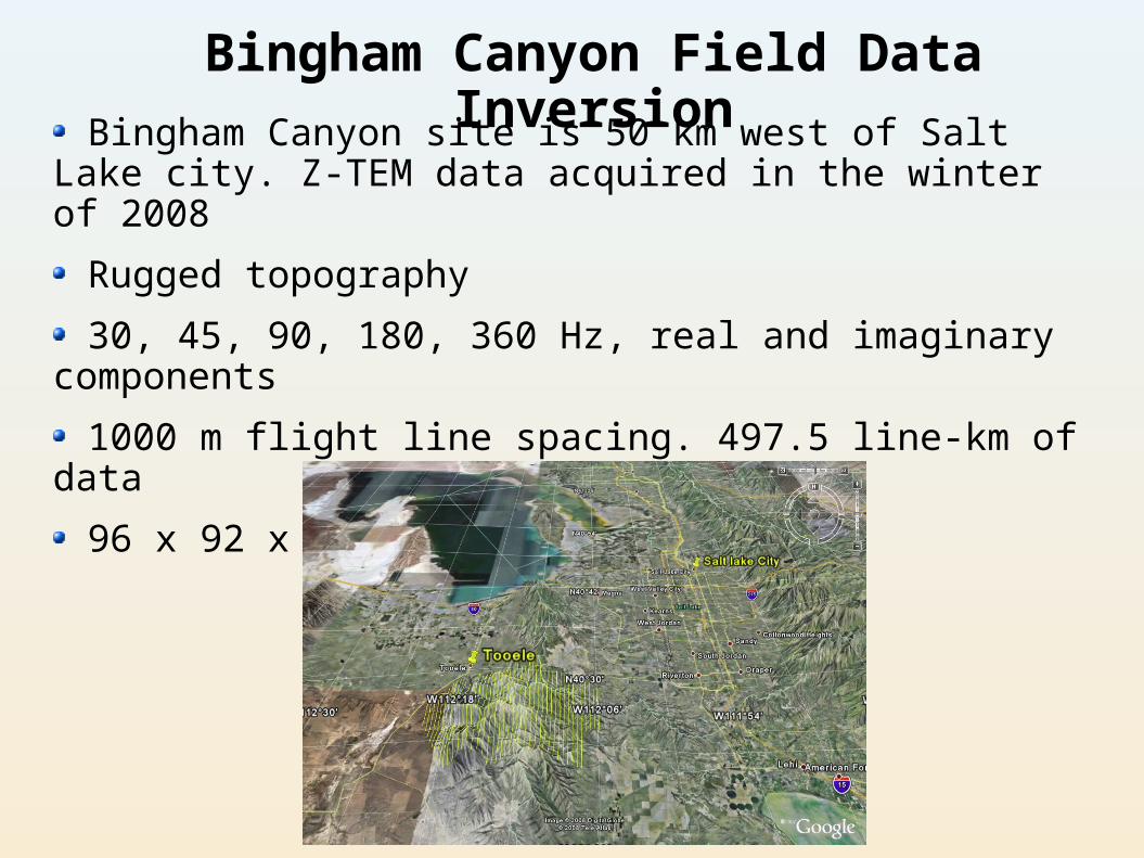
Bingham Canyon Field Data Inversion

Bingham Canyon site is 50 km west of Salt Lake city. Z-TEM data acquired in the winter of 2008

Rugged topography

30, 45, 90, 180, 360 Hz, real and imaginary components

1000 m flight line spacing. 497.5 line-km of data

96 x 92 x 95 cell mesh

Field Inversion Work flow

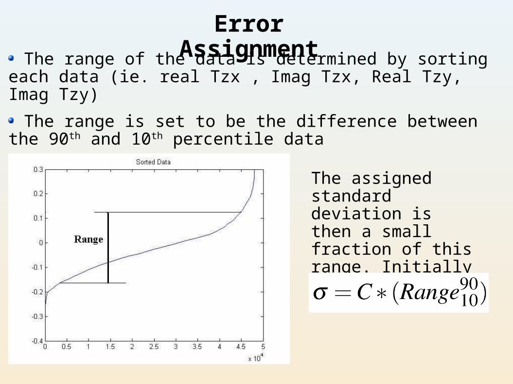
Error Assignment

The range of the data is determined by sorting each data (ie. real Tzx , Imag Tzx, Real Tzy, Imag Tzy)

The range is set to be the difference between the 90th and 10th percentile data

The assigned standard deviation is then a small fraction of this range. Initially C=0.125 for all frequencies.

Error Assignment

Invert each frequency of the data with the assigned standard deviations.

Adjust the constant C, until the final misfit achieves the target misfit

Misfit

Error Assignment

Inverting and adjusting the errors on each frequency separately gives the correct weighting of each frequency

Ensures that no frequency dominates inversion

45 Hz misfit – scale factor 1.50 180 Hz misfit – scale factor 1.90

Final Misfit Curve

Target Misfit: 1.52 E+06Final Misfit: 1.58 E+06

Misfit

30 Hz

Misfits

Observed data

Predicted data

45 Hz

Misfits

Observed data

Predicted data

90 Hz

Misfits

Observed data

Predicted data

180 Hz

Misfits

Observed data

Predicted data

360 Hz

Misfits

Observed data

Predicted data

Cut-offs (Below 1600m)Conductors > 0. 1 S/mResistors < 0.0001 S/m

Comparison of Inverted Model with Geology(Surface resistors and conductors)

Inverted Model Geologic Model

Comparison of Inverted Model with Geology(Surface resistors and conductors)

Inverted Model Geologic Model

Comparison of Inverted Model with Geology(Surface resistors and conductors)

Inverted Model Geologic Model

Comparison of Inverted Model with Geology(resistors and conductors below 1600m)

Inverted Model Geologic Model

Conclusions

Z-TEM data can be forward modeled

Inversion algorithm exists for inverting Z-TEM data

Inversion yields encouraging results on a synthetic model

Z-TEM technique has been applied to a field dataset and yields good results

Shows promise to find large scale structures at depth

Acknowledgements

Michael Zang and Exploration Syndicate, Inc.

Thank You