Inversion for rheological parameters from post-seismic surface

Geophys. J. Int. (2006) 164, 75–87 doi: 10.1111/j.1365-246X.2005.02803.x

GJI

Sei

smol

ogy

Inversion for rheological parameters from post-seismic surfacedeformation associated with the 1960 Valdivia earthquake, Chile

Francisco Lorenzo-Martın,1 Frank Roth2 and Rongjiang Wang2

1Institute of Geology, Mineralogy and Geophysics, Ruhr University Bochum, D-44780 Bochum, Germany. E-mail: [email protected] Potsdam (GFZ), Telegrafenberg, D-14467 Potsdam, Germany

Accepted 2005 September 12. Received 2005 August 10; in original form 2005 April 5

S U M M A R YData collected during two Global Positioning System campaigns in 1994 and 1996 across Chileand western Argentina (22 stations), in the area where the M w = 9.5 1960 May 22 Valdiviaearthquake took place, shows ground motion velocities that cannot be fully explained by theelastic strain accumulation during the interseismic phase of an earthquake deformation cycle.We use dislocation models to reproduce the observed velocities, with a 3-D source in a mediumwith one elastic layer overlying a Maxwell viscoelastic half-space, and a planar rupture surfacewith uniform coseismic slip. The reason for avoiding a more detailed and elaborated modelis that knowledge about the Valdivia earthquake source parameters and the area where theevent took place is poorly constrained. We focus, therefore, on examining the first-order post-seismic deformation, and ignore finer details about the heterogeneity of the Earth. By meansof a grid search inversion over more than a million different models, we derived the most likelyvalues for some of the medium and source parameters involved in the deformation process,namely viscosity (η), thickness of the elastic layer (D), average slip on the rupture surface(U 0) and the seismic coupling coefficient (χ). According to our study, the optimum values are:η = 1020 Pa · s, D = 46 km, U 0 = 15 m and χ = 96. A clear difference is seen between thesurface deformation caused by silent-slip on the rupture surface and the one caused by post-seismic relaxation processes, two possibilities proposed to explain the anomalous velocities.We find that the deformation associated with the 1960 Valdivia event can still be observed afterseveral decades and it is the most likely explanation for the velocity component that cannotbe explained by plate convergence. Our model also predicts that this deformation will stillbe measurable for several more decades. Our model reproduces the first-order pattern of themeasured GPS velocities, showing good agreement with recent finite-element studies, withthe advantage of simplicity and short computation time, allowing the extensive search for thebest-fitting model.

Key words: crustal deformation, dislocation, rheology, subduction, Valdivia, viscosity.

1 I N T RO D U C T I O N

With the establishment of the Global Positioning System (GPS),the accuracy of observations of time-dependent deformation of theEarth’s surface has significantly improved and continues to do so.Also, with an increasing number of sites providing continuous mea-surements and with more numerous Interferograms of SyntheticAperture Radar (InSAR), both the sampling rate and areal coveragein monitoring recent crustal movements have drastically increased.The data obtained can be used to extract more details about thespace–time development of tectonic processes, such as earthquake-related crustal deformations, and their basic rheological parameters,in a way that was not possible in the recent past. Post-seismic re-laxation, plate convergence or silent earthquakes, for example, can

now be studied with a high accuracy, despite the intrinsically lowmagnitude of the deformation involved.

Thanks to this recently acquired data accuracy, an interestingfeature can be observed around the area where the great 1960 Val-divia earthquake took place. GPS velocities for sites at latitudesfurther north have a direction parallel to the convergence betweenthe Nazca and South American plates, but observations from siteslocated close to the area of the earthquake are not coherent withdeformation caused by plate motion, but show anomalous seawardvelocities (Klotz et al. 2001; Khazaradze & Klotz 2003). The de-formation further north can be fully explained by the elastic strainaccumulation during the interseismic phase of an earthquake defor-mation cycle. These velocities agree with a full rate of convergence,in other words, a 100 per cent locking of the Andean Subduction

C© 2005 RAS 75

Dow

nloaded from https://academ

ic.oup.com/gji/article/164/1/75/632743 by guest on 08 January 2022

76 F. Lorenzo-Martın, F. Roth and R. Wang

Zone is needed to explain them. On the contrary, other processesmust be involved to produce the deformation observed in the areaof the Valdivia earthquake.

An explanation for this incoherence could be that the Valdiviaearthquake may still have an influence on the crustal motion in thisarea. Very large earthquakes, such as subduction events of Mw > 9,may induce large stresses in the mantle over a very broad region, andthe relaxation process may cause prolonged crustal deformation faraway from the coseismic rupture zone for several decades after theevent (Nur & Mavko 1974; Thatcher & Rundle 1984). Other possibleexplanations could be aseismic slip on the coseismic rupture surface(Nason & Weertman 1973), deep slip on its downdip prolongation oreven a combination of the three processes. Freymueller et al. (2000)and Zweck et al. (2002) interpreted the interseismic crustal motionobserved on the western Kenai Peninsula as resulting from a delayedor continuing post-seismic transient response of the 1964 Mw = 9.2Alaska earthquake. Savage & Plafker (1991) and Brown et al. (1977)attributed the immediate post-seismic relaxation after this event topost-seismic slip on the plate interface directly downdip from thecoseismic rupture. Kasahara (1975) suggested delayed strain releaseby aseismic faulting following the 1973 Nemuro-Oki earthquake,Japan. Fitch & Scholz (1971) explained post-seismic movementsafter the 1946 Nankaido earthquake, Japan, with a combination ofreversed slip on the coseismic rupture surface and delayed forwardslip on the deeper parts of the fault.

Deep slip was also suggested for the 1960 Valdivia earthquake(Linde & Silver 1989; Barrientos et al. 1992). However, these andother early works (Plafker & Savage 1970; Plafker 1972; Barri-entos & Ward 1990) tried to explain the observed deformationaround the area of the event using elastic models and, in most cases,including both co- and post-seismic deformation with the obser-vations. This approach cannot properly consider effects from vis-coelastic relaxation, which might not be negligible. Piersanti (1999)modelled uplift and uplift rates by means of a layered sphericalearth model with Maxwell rheology, but this work was based ondata from only two stations. Khazaradze et al. (2002) modelledGPS velocities as a combination of plate motion and continuouspost-seismic crustal deformation using a 3-D viscoelastic finite-element model. However, the geometry of the subduction zone inthis area is not well constrained by data, and the sensitivity of theresults to the model parameters remains unclear. Their work wascontinued by Hu et al. (2004), including a separate analysis ofdeformation due to the earthquake alone and deformation due tofault locking. Choosing two to three values for their model pa-rameters, they did a simplified check for the sensitivity of theirresults.

In this study we used data from 22 GPS stations across Chile andwestern Argentina (Fig. 1), collected during two GPS campaignsin 1994 and 1996 (Klotz et al. 2001; Khazaradze & Klotz 2003).We modelled the measured deformation by means of software byWang et al. (Wang 1999; Wang et al. 2003, 2005). This method andits implementation have several advantages, such as speed and highprecision. Also, the effect of gravity was included in a consistentway, with an improved algorithm that corrects a mistake in formerworks by other authors (Fernandez & Rundle 2004; Wang 2005;Wang et al. 2005). This software also allows us to consider co-and post-seismic deformation processes in an adequate manner. Itsspeed also allows us to carry out a systematic global search for anoptimum model with a fairly broad parameter space. These facilitiesare used to search for an explanation for the anomalous velocitiesaround the earthquake’s location. We also carried out an inversionfor rheological and structural parameters in this area using the GPS

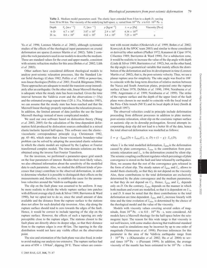
Figure 1. Map of the study area. The triangles show the 22 GPS sites usedfor this work. Thin arrows and error ellipses show the measured annual ve-locities (Klotz et al. 2001; Khazaradze & Klotz 2003). Numerical values forthese velocities are shown in Table 1. The thick arrows display the annualvelocities obtained by means of the best-fitting model. The dashed-line rect-angle shows the projection of the rupture surface used for calculations. Thethick black line shows the position of the Chile trench. Squares display themost important cities. White dots display the seismicity (events with mag-nitude at least 5) between 1961 and 1981 from the South American SISRACatalog (Askew & Algermissen 1985). Stars show the location of the epi-centre of the 1960 Valdivia earthquake after Talley and Cloud (number 1,Talley & Cloud 1962), Cifuentes (number 2, two subevents, Cifuentes 1989)and Krawczyk & the SPOC team (number 3, Krawczyk & the SPOC team,2003). Areas delimited by dashed lines (A, B and C) display latitude intervalsfor the panels shown in Fig. 5.

data, and found the most likely values for these parameters and theirreliability. We also estimate the time for which deformation due tothe earthquake will still be measurable.

2 T H E 1 9 6 0 VA L D I V I A E A RT H Q UA K E

The Valdivia earthquake of 1960 May 22 is until now the largestevent ever recorded by a seismic network. The main shock consistedof two subevents adding up to a moment magnitude of 9.5 (Kanamori1977). The destruction area extended for more than 800 km in a N–S direction. Surface deformation related to the earthquake, includ-ing both uplift and subsidence relative to sea level, was observedover an even larger area of southern Chile (Talley & Cloud 1962,pp. 57–58; Alvarez 1963; Plafker & Savage 1970).

Despite the intensive scientific and engineering studies madeshortly after the disaster, surprisingly little has been published

C© 2005 RAS, GJI, 164, 75–87

Dow



Rheological parameters from post-seismic deformation 77

concerning the generative mechanism of this event. Nor is muchinformation about the area of occurrence of the event. Most studiesrelated to the South American Subduction Zone have been carriedfor latitudes further north (Jordan et al. 1982; Cahill & Isacks 1992;Araujo & Suarez 1994) or, in the best of the cases, only over thenorthernmost part of the Valdivia rupture area (Tichelaar & Ruff1991; Bohm et al. 2002; Krawczyk & the SPOC team 2003; Luthet al. 2003). In the following sections, we briefly present backgroundinformation relevant to our work, that is, the subduction zone andthe source mechanism of the event and its geometry.

2.1 Tectonic setting and seismicity

The 1960 Valdivia earthquake sequence ruptured about 1000 km ofthe southernmost section of the South American Subduction Zone.In this region, the Nazca Plate is being subducted beneath SouthAmerica along the Peru–Chile trench at a rate of 78 mm a−1, ac-cording to the analysis of seafloor palaeomagnetic data (DeMetset al. 1994; Somoza 1998). Space-geodetic estimates provide avalue considerably lower for the convergence velocity (66 mm a−1

(Angermann et al. 1999); 69 mm a−1 (Norabuena et al. 1998, 1999).These results are based on observations over a relatively short timespan, and may therefore be affected by short-term deformation pro-cesses, while palaeomagnetic studies provide only a long-term av-erage velocity that may not be representative of the current conver-gence rate. We favoured for this reason the use of the results fromthe recent geodetic studies.

2.2 Mechanism and location

There were no fault displacements at the surface to provide directgeological evidence as to the orientation and sense of slip on thecausative fault or faults (Alvarez 1963). Similarly, the seismologicaldata was generally inadequate to permit either reliable focal mech-anism solutions or precise delineation of the focal region (Plafker& Savage 1970). No fault-plane solution is available for the mainshock of the 1960 sequence because the first arrivals were maskedon most seismograms by the large foreshock that immediately pre-ceded it (Cifuentes 1989).

Precise location of the epicentre of the main shock was not possi-ble for the same reason. The U.S. Coast and Geodetic Survey locatedthe epicentre on the continental shelf, approximately 80 km offshorefrom the coastline and 60 km west of Isla Mocha (38.30◦S, 74.30◦W,(Talley & Cloud 1962); see Fig. 1 for these geographical locations).Cifuentes (1989) relocated the sequence of the earthquake using themaster-event technique. According to her work, the two subeventsof the main shock were relocated to 38.05◦N, 72.34◦W and 38.16◦N,72.20◦W. Recently, Krawczyk & the SPOC team (2003) presentedfor the first time the slab geometry of this area, based on a near-vertical seismic reflection experiment, and proposed a new locationat 73.08◦W. This recent work gives an idea of how many aspects ofthis earthquake are still not well known.

2.3 Coseismic slip on the rupture surface

Plafker & Savage (1970) and Plafker (1972), by means of the dis-location analysis of vertical surface deformation several years afterthe earthquake, found that the most plausible model for the Valdiviaearthquake would be a fault with an average slip of about 20 m.Strain modelling suggested, however, that the slip required to sat-isfy the surface displacement may be as large as 40 m. Kanamori& Cipar (1974) estimated an average dislocation of 24 m from theanalysis of a long-period strain seismogram. Barrientos & Ward

(1990) employed surface deformation data from more than 300 datapoints to investigate the slip distribution on the rupture surface. Sev-eral slip peaks appeared on this surface, in some cases exceeding40 m. However, the average repeat time has been estimated to be128 ± 31a (Nishenko 1985) and, by the present convergence rate ofthe Nazca and South America plates, much less slip would accumu-late during such a period.

2.4 Rupture surface geometry

The Wadati-Benioff zone is delineated well enough to infer the dipof the subducting Nazca Plate only in the Arauco Peninsula region,the northern section of the rupture area of the Valdivia earthquake.There, the Wadati-Benioff zone does not extend deeper that 160 km.The Nazca Plate in the Arauco Peninsula region dips at a shallowangle of about 15◦ to a depth of 40 km, where it steepens to amoderate dip of about 30◦ to reach a depth of about 125 km beneaththe volcanoes (Bohm et al. 2002; Krawczyk & the SPOC team 2003;Luth et al. 2003). The average dip might be larger than for the AraucoPeninsula region, as the dip in the region north of the 1960 rupturearea (Jordan et al. 1982; Cahill & Isacks 1992). It might also be less,because of the increase in buoyancy due to the southward decreasein the age of the oceanic lithosphere being subducted. Plafker &Savage (1970) estimated the dip angle to be of the order of 35◦.Plafker changed this value to 20◦ in a later work (Plafker 1972).

The width of the rupture surface of the Valdivia earthquake ispoorly constrained. An approximate measure is obtained from thedip of the Nazca Plate in the Arauco Peninsula region and the proba-ble depth range of faulting. The width of the aftershock distribution,excluding the events close to the trench axis as they are not on themain thrust zone, yields an approximate width for the rupture areaof 140 km (Cifuentes 1989). However, the depth of aftershocks arepoorly determined, and thus the depth range is not well constrained.

The rupture length of the main shock is also not well known.In contrast to the northern endpoint, the southern endpoint is notclearly determined, due to the lack of information south of 45◦S. Inany case, the sites we used for our analysis are located around itsnorthern half (Fig. 1). Thus, the exact southern end of the rupture isnot critical for our study. Benioff et al. (1961) made the first deter-mination of fault length from instrumental data, suggesting a valueof 960–1200 km. The distribution of aftershocks during the firstmonth leads to a value of 930 km (Cifuentes 1989). An estimate ofrupture length can also be obtained from the extent of crustal defor-mation. The southernmost point of vertical displacement measuredby Plafker & Savage (1970) is at 45.21◦S, but the extent of verticaldisplacement could reach as far south as the Taitao Peninsula, wherea few centimetres of uplift were reported after the earthquake. Therupture length can be estimated as the distance between the initia-tion of the earthquake and the southern limit of crustal deformation.This length is 800 km to the southernmost measured point, and 920km to the Taito Peninsula. According to this, Cifuentes (1989) pro-posed a value of 920 ± 100 km for the rupture length, within therange of values previously presented (Benioff et al. 1961; Press et al.1961).

3 T H E M O D E L L I N G

For our study of the post-seismic deformation associated with the1960 Valdivia earthquake, we use observations from 22 sites fromthe SAGA (South American Geodynamic Activities) GPS network(Klotz et al. 2001; Khazaradze & Klotz 2003). The stations cover thenorthernmost part of the rupture area of the 1960 event (Fig. 1). Thevalues used are listed in Table 1. The collected data was processed

C© 2005 RAS, GJI, 164, 75–87

Dow




Table 1. GPS site velocities from the SAGA network used in the modelling (Klotz et al. 2001; Khazaradze & Klotz 2003).

Station ID Longitude [◦] Latitude [◦] W–E vel. [mm a−1] 1σ error [mm a−1] S–N vel. [mm a−1] 1σ error [mm a−1] correl. coeff.

ANTU 288.3745 −37.3358 16.4 2.1 1.3 2.0 0.05AUMA 291.4048 −37.6065 −1.9 1.9 −4.0 2.0 0.01BARI 288.5865 −41.1321 −11.7 2.0 −3.2 2.2 0.09CALF 286.6116 −39.7539 16.3 2.0 7.4 2.1 0.12CEPI 289.3679 −40.2494 −6.7 2.0 −1.2 2.1 0.07

CHOL 287.5584 −42.0279 −5.8 2.0 0.6 2.2 0.12CHOS 289.6855 −37.3608 5.9 1.9 −6.7 2.0 0.04COMA 289.7824 −41.0363 −9.5 2.0 1.0 2.2 0.06ELCH 291.1123 −39.2906 −3.4 1.9 2.5 2.1 0.02EPUY 288.5956 −42.1405 −7.6 2.0 0.5 2.2 0.10FTRN 287.6233 −40.1304 −0.3 2.0 8.6 2.1 0.10GUAB 285.9728 −41.8063 16.2 2.0 9.2 2.2 0.15LAAM 289.9449 −38.8360 −1.1 1.9 −6.0 2.1 0.04LINC 287.5962 −40.6233 −8.2 2.2 −2.2 2.2 0.08PAST 288.5272 −39.5835 −3.4 2.0 −0.4 2.1 0.08PEHO 288.9261 −38.5967 −3.0 1.9 −5.0 2.1 0.06PPUY 288.0646 −40.7007 0.3 2.0 2.2 2.2 0.10PSAA 286.5942 −38.7788 19.5 2.0 8.1 2.1 0.10PTMT 287.0523 −41.4628 −0.6 1.9 4.8 2.2 0.14PUAW 287.6075 −38.3383 2.9 2.1 2.3 2.1 0.05PUCA 286.2800 −40.5468 27.6 2.0 8.5 2.2 0.13RALU 287.6879 −41.3785 0.6 2.0 3.3 2.2 0.12

and transformed to a fixed South America reference frame (Klotzet al. 2001).

The mean value of position residuals for these stations, reflectingthe achieved regional network precision, is of the order of 2 mmand 5–7 mm for horizontal and vertical displacement, respectively.Since the expected surface uplift in the Andean Subduction Zonedoes not exceed 2 mm a−1, two observations separated by 2 years arenot sufficient to resolve the possible vertical motions with adequateconfidence. For this reason we only considered the two horizontalcomponents of the deformation in our work.

As already mentioned, different approaches have been used byother authors to model the subduction zone where the Valdivia earth-quake took place. The most important conclusions from their analyseare:

(1) The predicted deformation is notably sensitive to the distribu-tion of slip on the rupture surface (Linde & Silver 1989; Barrientos& Ward 1990). However, external constraints are needed to realis-tically resolve this parameter.

(2) Effects due to post-seismic relaxation are not negligible.When considered, models with viscosity in the range of 1019

(Khazaradze et al. 2002; Hu et al. 2004) to a few times 1020 Pa · s(Piersanti 1999) provide good results for this area.

(3) The geometry of the rupture surface is an important parameter(Klotz et al. 2001; Khazaradze et al. 2002; Khazaradze & Klotz2003; Hu et al. 2004). However, external information is required todescribe it. Unfortunately, such information is scarce or not availablein detail for the Valdivia area.

(4) The structure of the medium layering has also a significant ef-fect on the modelled data (Piersanti 1999). Lateral inhomogeneitiesalso have a significant effect on the deformation field (Khazaradzeet al. 2002; Hu et al. 2004). However, the model details might notbe resolved by the available data.

(5) Sensitivity studies for the parameters involved in the mod-elling have been seldom conducted.

(6) Trade-off between different parameters has been discussedbriefly in earlier works (Hu et al. 2004), but no further testing hasbeen carried out so far.

With this factors in mind, we performed an inversion on foursource and medium parameters for the Valdivia earthquake and thearea where it took place: the average coseismic slip on the rupturesurface U 0, the viscosity of the underlying viscoelastic half-spaceη, the thickness of the overlying elastic layer D and the seismiccoupling coefficient χ (Scholz & Campos 1995). Fig. 2 shows aschematic representation of the fault geometry and the medium usedin the modelling. We model the deformations using an elastic layerover a viscoelastic half-space with linear Maxwell rheology. Thisrheological model is a reasonable simplification that neverthelessrepresents the properties of the crust and upper mantle appropri-ately. Such a medium has been widely used in earlier publications(Cohen 1980a,b; Rundle 1982; Cohen 1994; Fernandez et al. 1996;

Figure 2. Schematic representation of the fault geometry and medium usedin the modelling. On the vertical section, the points on the rupture surfacerepresent the point sources into which the extended surface is discretized.(Wang et al. 2003, 2005).

C© 2005 RAS, GJI, 164, 75–87

Dow




Table 2. Medium model parameters used. The elastic layer extended from 0 km to a depth D, varyingfrom 30 to 98 km. The viscosity of the underlying half-space, η, varied from 1018 Pa · s to 8.0 · 1022 Pa · s.

Depth Vp [m s −1] Vs [m s −1] ρ [kg m−3] λ = µ [Pa] Viscosity [Pa·s]

0–D 6.7 × 103 3.87 × 103 2.9 × 103 4.34 × 1010 –D–∞ 8.0 × 103 4.62 × 103 3.4 × 103 7.25 × 1010 η

Yu et al. 1996; Lorenzo Martın et al. 2002), although systematicstudies of the effects of the rheological input parameters on crustaldeformation are sparse (Lorenzo Martın et al. 2002). Table 2 com-piles the rock parameters used in our models to describe the medium.These are standard values for the crust and upper mantle, consistentwith seismic refraction studies for this area (Bohm et al. 2002; Luthet al. 2003).

Other authors have considered different rheological models toanalyse post-seismic relaxation processes, like the Standard Lin-ear Solid rheology (Cohen 1982; Pollitz et al. 1998) or power-law,non-linear rheologies (Pollitz et al. 2001; Freed & Burgmann 2004).These approaches are adequate to model the transient creep immedi-ately after an earthquake. On the other side, linear Maxwell rheologyis adequate when the steady state has been reached. Given the timeinterval between the Valdivia event and the observations (∼35a)and the estimated average repeat time (128 ± 31a, Nishenko 1985),we can assume that the steady state has been reached and that theMaxwell linear rheology properly reproduces the relaxation process.In addition, the limited amount of data justifies the use the linearMaxwell rheology instead of more complicated models.

We used our own software based on dislocation theory (Wanget al. 2003, 2005) for the calculation of the time-dependent defor-mation field produced by dislocation sources embedded in a mixedelastic/inelastic layered half-space. This software uses the elastic–viscoelastic correspondence principle (e.g. Christensen 1982,pp. 45–46), which states that a linear viscoelastic boundary-valueproblem can be solved by adopting the associated elastic solutionsin which the elastic moduli are replaced by the Laplace or Fouriertransformed complex moduli. The time-domain solutions are thenobtained using the inverse Fast Fourier Transform.

For the inversion, we performed a parameter-space grid searchon the four parameters of interest. Besides their most likely values,we also obtained information about the sensitivity of the modelleddata to each parameter. Also, we studied the different kinds of pro-cesses that (may) contribute to the observed deformation, in orderto determine whether it is possible to distinguish their effects on themeasurements and, therefore, to establish the cause for the anoma-lous velocities around the Valdivia earthquake area.

The slip on the fault plane was assumed to be uniform. It maybe more realistic to divide the whole rupture surface into patcheswith different average slip (Linde & Silver 1989; Barrientos & Ward1990), but we opted not to do so, since the small amount of dataavailable and the distance from the rupture surface to the stationsdoes not allow for such detailed slip inversion. Also, slip along therupture surface should tend to zero towards the edges of the fault.Hence, it would be correct to include tapering of the slip on therupture surface. However, the effects of such a tapering are onlyperceptible close to the rupture edges. The stations closest to thefault plane are directly above its deeper edge, so that their distancefrom to the rupture edges is over 40 km. The tapering in the slipdistribution would not have any visible effect on the observationpoint.

The size and orientation of the fault plane was also fixed, in orderto avoid making our analysis too extensive. The rupture surface hadan area of 850 × 130 km2, dipping 20◦E. These values are consis-

tent with recent studies (Oleskevich et al. 1999; Bohm et al. 2002;Krawczyk & the SPOC team 2003) and similar to those consideredor derived by other authors (Plafker 1972; Kanamori & Cipar 1974;Cifuentes 1989; Barrientos & Ward 1990). For a subduction zone,it would be realistic to increase the value of the dip angle with depth(Linde & Silver 1989; Barrientos et al. 1992), but, on the other hand,the dip angle is a geometrical variable that mainly affects the distri-bution of the deformation and less its development in time (LorenzoMartın et al. 2002), that is, the post-seismic velocity. Thus, we use aplanar rupture area for simplicity. The rake angle was fixed to 108◦

to coincide with the long-term direction of relative motion betweenthe Nazca and South American plates, projected onto the rupturesurface (Chase 1978; DeMets et al. 1990, 1994; Norabuena et al.1998; Angermann et al. 1999; Norabuena et al. 1999). The strikeof the rupture surface and the depth of the upper limit of the faultplane were chosen in our model to coincide with the local trend ofthe Peru–Chile trench (N8◦E) and its local depth (4 km) (Smith &Sandwell 1997).

The observed velocities could in principle include deformationproceeding from different processes in addition to plate motion:post-seismic relaxation, silent slip on the coseismic rupture surfaceor aseismic slip on its downdip prolongation. Several attempts in-corporating deep slip did not lead to a better fit of the data, hencethe total observed deformation was modelled as follows:

�x = χ · �xplate(D) + �xrelax(U0, η, D) + (1 − χ ) · �xss(D), (1)

where �x is the total modelled deformation, �xplateis the deformationcaused by plate convergence, �xrelax is the contribution from post-seismic relaxation and �xss is the deformation created by silent slip.The seismic coupling coefficient regulates which percentage of plateconvergence is stored on the fault and later released by earthquakes.Here, we assume that the rest of the convergence gets released inthe form of silent slip. The steady nature of �xplate and �xss allows tomodel them elastically, so that they do not depend on the viscosity.Also, these contributions to the total deformation are exclusivelydetermined by the plate convergence and the medium parameters,so that they do not depend on U 0. Hence, �xplate and �xss dependsonly on D. On the contrary, �xrelax depends on the manner in whichboth medium and event are modelled, so that it is dependent on U 0,η and D. It must be noted that the three contributions to the totaldeformation are time dependent. �xplate and �xss increase linearly withtime and the time evolution of �xrelax is determined by the choice ofthe rheological model and the value of the viscosity.

Models with viscosity values covering several orders of mag-nitude, from 1018 Pa · s to 8.0 · 1022 Pa · s, were considered. Allmodels have a Maxwell rheology for the half-space below the seis-mogenic layer. The reason for this wide range is that viscosity isnot well known, with some studies showing that traditional standardvalues used in simulations may be incorrect by up to one order ofmagnitude (Vermeersen et al. 1998). Previous inferences for thisparameter in the area of the Valdivia earthquake range from3 · 1019 Pa · s (Khazaradze et al. 2002; Hu et al. 2004) to sev-eral times 1020 Pa · s (Piersanti 1999). In addition, the averageviscosity of the mantle has been estimated to be 1021 Pa · s from

C© 2005 RAS, GJI, 164, 75–87

Dow




post-glacial rebound (James et al. 2000) and rotational dynamicstudies (Lambeck 1980).

For each viscosity value, the thickness of the elastic layer wasvaried between 30 and 98 km. Tichelaar & Ruff (1991) estimated thedepth of seismic coupling in Chile to be 48–53 km, while Oleskevichet al. (1999) proposed 40–50 km. Recent seismic refraction studiespropose a crustal thickness of at least 35 km at ∼38.15◦S (Bohmet al. 2002; Krawczyk & the SPOC team 2003). However, somemodelling approaches by other authors considered a much thickerelastic layer (Piersanti 1999).

It must be noted at this point that we are limited to modellinghomogeneous horizontal layers. Hence, the thickness of the elasticlayer may not be directly interpreted as the thickness of the crustin the area where the earthquake occurred. The latter shows stronglateral variations, especially in the trench-perpendicular direction.Rather, our elastic layer thickness reflects the depth range where bothoceanic and continental plates are coupled and where the materialbehaves elastic/brittle, so that seismicity can occur.

We considered a range of different values for the average slip onthe rupture surface, between 10 and 45 m. Different authors considerdifferent values for this parameter, ranging from 17 m (Barrientos& Ward 1990) to 40 m (Plafker & Savage 1970). With the rupturesurface and medium rock parameters of our model, a coseismicaverage slip of at least 40 m is required to fit the moment magnitude,hence the high upper limit for the values that we regard as possible.

No specific study has been done for the state of coupling of theChilean Subduction Zone at the latitudes in this work. It is clear thatthis subduction zone, with young lithosphere subducting rapidly,must be strongly coupled and has a highly compressive strain regime(Uyeda 1982; Scholz & Campos 1995; Klotz et al. 2001; Conradet al. 2004). Therefore, the seismic coupling coefficient (reflectingthe degree of mechanical coupling at the plate interface) for thissubduction zone must be close to 1. We consider a number of dif-ferent values for the seismic coupling coefficient, ranging from 1,meaning totally locked (Klotz et al. 2001), down to 0.65. Lowervalues are not reasonable.

Altogether, a total number of 1 224 720 different models wereconsidered.

To evaluate the fit between the models and the data, we calculatedthe deviation as follows:

� =22∑

i=1

[(xi − xGPS

i

σxi

)2

+(

yi − yGPSi

σyi

)2], (2)

where (xGPSi , yGPS

i ) are the measured displacement at the ith stationin the S–N and W–E direction, respectively, (σxi , σyi ) are the corre-sponding error estimations and (xi, yi) are the respective modelleddisplacement values.

4 R E S U LT S A N D D I S C U S S I O N

4.1 Parameter inversion

From the grid search we found that the best-fitting model has anelastic layer D = 46 km overlying a viscoelastic half-space with aviscosity of η = 1020 Pa · s, an average slip of U 0 = 15 m and aseismic coupling coefficient of χ = 0.96. This set of parameters isrepresented by small white circles in Figs 3 and 4.

The soundness of these inversion results was tested by means of aMonte Carlo error propagation analysis. This is a statistically robustapproach to evaluate the stability of the parameters’ estimation byreiterating the inversion for sets of potential deformation rates at the

GPS sites, taking into account the uncertainties in the velocity val-ues. We considered two times 550 random sets of velocities fallinginto the 1σ and 2σ GPS error ellipses. They led to the values respec-tively shown by crosses and dots in Figs 3 and 4. The results must notbe mistaken with the analysis of the deviation curves. The latter onlyprovides a qualitative estimation of the dependence of the deviationon the considered parameter and cannot be used to extract a confi-dence interval. The Monte Carlo method offers alternative possiblebest-fitting models when inaccuracies in the data are considered.It propagates the confidence ellipses in the GPS measurements tothe determination of the minimum deviation and, therefore, to theestimation of the most likely value for the parameters.

The displacements calculated by means of the best-fitting modelare shown in Fig. 1 by thick-line vectors. The average differencebetween model velocities and GPS observations is 6 mm a−1, com-parable to the 3σ errors of the GPS velocities. If we only considerthe stations south of latitude 38◦S, the differences are reduced to4 mm a−1, the same value obtained by Hu et al. by means of theirfinite-element modelling (Hu et al. 2004).

Fig. 3 shows the dependence of the deviation between observa-tions and predictions on the variation of each parameter. The upperpanel shows the effect of the elastic layer thickness. For low valuesin this variable, a moderate variation leads to sharp and strong vari-ations in the deviation. The origin of this is the discretization of theextended source into a finite number of point sources. (Wang et al.2003, 2005). The change in the depth for the elastic to viscoelasticboundary implies a change in the medium properties for a numberof point sources (see Fig. 2), hence the deviation changes abruptlyrather than continuously. The depths of the deepest point sourcesare shown as vertical dashed lines to illustrate this problem. The ob-tained result of D ≤ 46–48 km may be interpreted as the thicknessof the continental crust under the GPS sites, consistent with valuederived from seismic refraction data (Bohm et al. 2002; Krawczyk& the SPOC team 2003). This result is also consistent with the depthof coupling between the Nazca and the South American plates, asinferred from the distribution of interplate seismicity (Tichelaar &Ruff 1991).

The value of η = 1020 Pa · s for the viscosity led to the best fitof the data (second panel, Fig. 3). This result agrees with previousworks for this region (Piersanti 1999) and also with other studiesdealing with the viscosity of the upper mantle (Vermeersen et al.1998). Our result is very well constrained according to the MonteCarlo analysis. The local minimum for η = 3 · 1018 Pa · s correspondsto a viscosity, which is usually considered too low.

A best estimate of the coseismic slip U 0 = 14–16 m (thirdpanel, Fig. 3) is similar to the one deduced by Barrientos & Ward(Barrientos & Ward 1990) for their uniform slip planar model, butmuch smaller than the patches of high displacement of their variableslip model. Other works consider or derive comparable values forthis parameter (Khazaradze et al. 2002), although some authors sug-gest the possibility of a much larger average slip (Plafker & Savage1970). We discuss this possibility in Section 4.2.

The best-fitting model had a seismic coupling coefficient ofχ = 0.94–0.98 (fourth panel, Fig. 3), meaning that the Chileansubduction zone is 94–98 per cent locked. This is a reasonable re-sult, being that the Chilean subduction zone is an area with a highlycompressive strain regime (Scholz & Campos 1995; Klotz et al.2001; Conrad et al. 2004).

According to the error propagation analysis, these parameter es-timates are stable and reliable when considered independently. Es-pecially, the value for the viscosity in this area remains unchangedfor sets of GPS velocities randomly distributed inside their 2σ error

C© 2005 RAS, GJI, 164, 75–87

Dow




Figure 3. Dependence of the deviation (�, eq. 2) against each parameter. From top to bottom: elastic layer thickness (D), viscosity (η), coseismic average slipon the rupture surface (U 0) and seismic coupling coefficient (χ ). For each panel, the three variables that are not considered were fixed to the values that led tothe best-fitting model (see Table 3). Vertical dashed lines on the upper panel display the depth of the deepest point sources into which the rupture surface wasdiscretized. The white circle in each panel shows the position of the minimum, crosses and dots, respectively, display values for models resulting from the 1σ

and 2σ error propagation analysis.

ellipses. The seismic coupling coefficient, on the other hand, is lesswell resolved. Given the uncertainty in the determination of thisparameter, we can only conclude that the data is consistent with ahighly locked fault.

We performed two inversions from models under two specialrestrictions: first, the subduction zone was set to be fully locked

(χ = 1), such that viscoelastic relaxation and interseismic elas-tic strain were the only processes causing deformation. Second,models with no post-seismic relaxation processes were considered.The results from these inversions are summarized in Table 3, to-gether with the results when all deformation types were present.The results show that including post-seismic relaxation improves

C© 2005 RAS, GJI, 164, 75–87

Dow




Figure 4. The trade-off between pairs of the studied parameters. For each panel, the two variables that are not considered were fixed to the values that ledto the best-fitting model (see Fig. 3 and Table 3). The field displayed is �′ = 30 · ln(�/�min), where � is the deviation between the modelled and observedvelocities. The white circles show the position of the minimum, crosses and dots, respectively, display parameter values for models resulting from the 1σ and2σ error propagation analysis. Isolines display contours for �′ equal to 1, 3, 10 and 30.

the fit to the observed GPS data. If we assume that post-seismic re-laxation is not taking place, or that its influence cannot be observedon the measured deformation, the deviation between modelled andobserved data is 87 per cent larger. On the other hand, excludingsilent slip also leads to a good fit between modelled and observeddata. This is an anticipated result, since the inversion for the generalcase already suggested that the subduction zone is almost completelylocked.

Finally, we also carried out an inversion using the convergencerate of 78 mm a−1 provided by palaeomagnetic studies instead of the66 mm a−1 from geodetic studies. The results from the inversion donot change, with the exception of the value for the seismic coupling

coefficient (see Table 3). Increasing the convergence rate impliesthat the interseismic deformation caused by plate convergence islarger. As a consequence, in order to maintain the goodness of thefit, the contribution of plate motion to the total deformation mustbe reduced, hence the seismic coupling coefficient must be smaller(see eq. 1).

4.2 Trade-off

Fig. 4 shows the trade-off between pairs of studied parameters. Foreach panel, the two variables that are not considered were fixed tothe value that led to the best-fitting model (see Fig. 3 and Table 3). To

C© 2005 RAS, GJI, 164, 75–87

Dow




Table 3. Parameter values corresponding to the best-fitting models for four different assumptions about the origin of the deformation. First(x plate, x relax, xss), the observed velocities is fitted by deformation from plate motion, post-seismic viscoelastic relaxation and silent slip on therupture surface. Second (x plate, x relax), the seismic coupling coefficient is fixed to χ = 1, meaning that no silent slip takes place. Third, weassume that no relaxation process exists (x plate, xss), or that its effect cannot be observed on the measured velocities. Finally, we consider theNazca–South America convergence rate from palaeomagnetic studies (DeMets et al. 1994).

Contributions to deformation x plate, x relax, xss x plate, x relax x plate, xss x plate, x relax, xss (NUVEL-1A)

Elastic layer thickness (D) [km] 46 82 46 46Half-space viscosity (η) [Pa · s] 1.0 · 1020 9.0 · 1018 – 1.0 · 1020

Average slip (U 0) [m] 15 13 – 15Seismic coupling coefficient (χ ) 0.96 (1.0) 0.72 0.89

Deviation from the observed GPS data (�) 255.0109 278.3046 476.5012 255.0987

facilitate the analysis, the field displayed is �′ = 30 · ln (�/�min).Also, the results from the 1σ and 2σ error propagation analysis areshown.

No clear trade-off between pairs of variables is observed, withthe exception of viscosity and coseismic average slip. In this case,models with η = 2 · 1020 Pa · s and U 0 = 26–31 m, as well as modelswith η = 3 · 1020 Pa · s and U 0 = 41–45 m also provide a good fitto the GPS data. A linear regression of the viscosity on the average

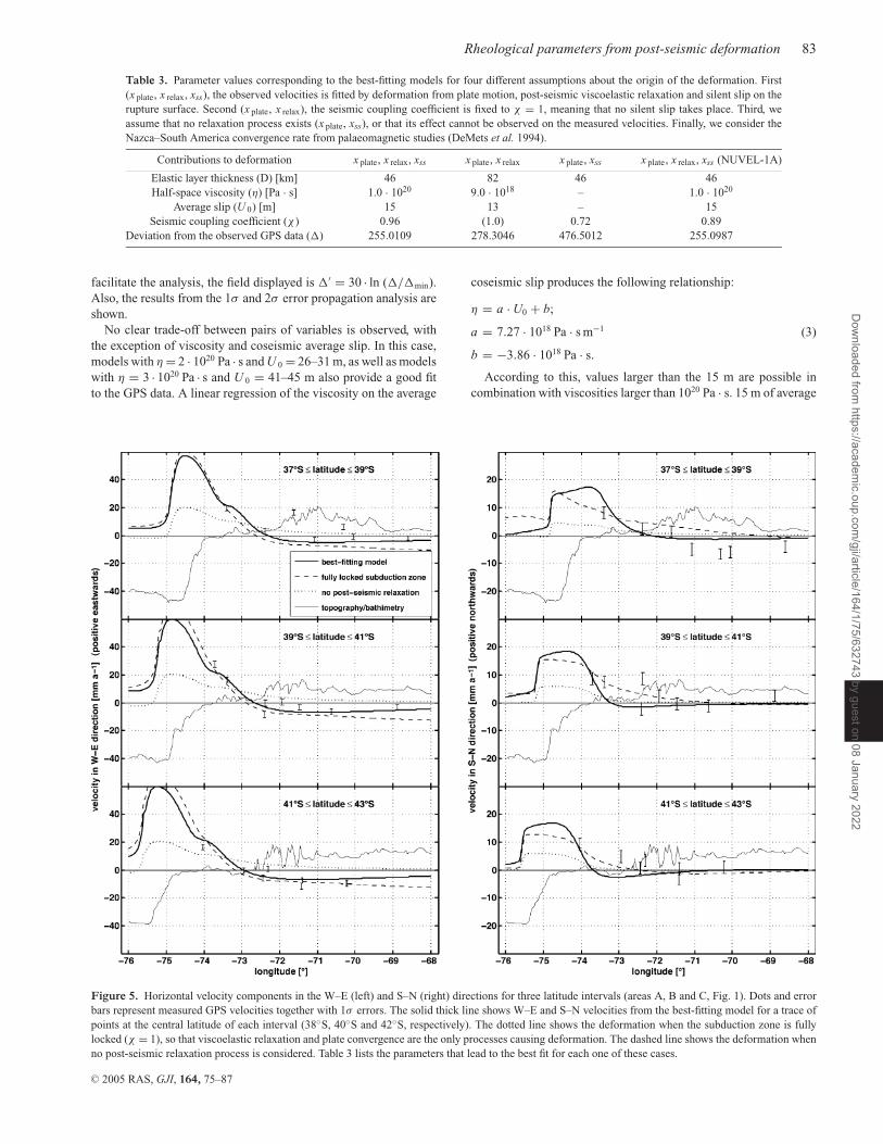
Figure 5. Horizontal velocity components in the W–E (left) and S–N (right) directions for three latitude intervals (areas A, B and C, Fig. 1). Dots and errorbars represent measured GPS velocities together with 1σ errors. The solid thick line shows W–E and S–N velocities from the best-fitting model for a trace ofpoints at the central latitude of each interval (38◦S, 40◦S and 42◦S, respectively). The dotted line shows the deformation when the subduction zone is fullylocked (χ = 1), so that viscoelastic relaxation and plate convergence are the only processes causing deformation. The dashed line shows the deformation whenno post-seismic relaxation process is considered. Table 3 lists the parameters that lead to the best fit for each one of these cases.

coseismic slip produces the following relationship:

η = a · U0 + b;

a = 7.27 · 1018 Pa · s m−1

b = −3.86 · 1018 Pa · s.

(3)

According to this, values larger than the 15 m are possible incombination with viscosities larger than 1020 Pa · s. 15 m of average

C© 2005 RAS, GJI, 164, 75–87

Dow




rupture slip corresponds to a moment M 0 = 7.2 · 1022 N·m and,therefore, a magnitude Mw = 9.2 using the Kanamori relationship,much lower than the actual Mw = 9.5. Consistency with the lattervalue would imply a seismic moment of M 0 = 2.24 · 1023 N·m, and,therefore, an average coseismic slip of U 0 = 40 m, which conflictswith recurrence time and convergence rate data (Nishenko 1985;DeMets et al. 1994; Somoza 1998). There are two possible expla-nations for this problem. First, this may be an indication that thedistribution of slip on the rupture surface should be modelled non-uniformly. To check this, a better areal coverage could be very usefulwhen inverting for the distribution of slip. The second possibility isthat the average slip on the rupture surface is larger than the 15 mobtained in this study, implying a larger viscosity. Data from a latercampaign will be useful in gaining a better insight into the time de-velopment of the relaxation process, so that higher viscosity valuescould be confirmed or ruled out.

4.3 Horizontal velocity components

Fig. 5 shows the horizontal velocities along the W–E (left panels) andS–N (right panels) directions for three latitude intervals. The dotsare the observed deformation data for the stations correspondingto each interval, together with 1-σ error bars. The solid thick lineshows the W–E and S–N velocities for the best-fitting model for atrace of points at the central latitude of each interval (38◦S, 40◦S and42◦S, respectively, see also Fig. 1). For the W–E velocities, the fit isin general good, with our best-fitting model reproducing the trendshown by the GPS velocities. In the case of the S–N velocities, thebest fit occurs at the two southernmost profiles, although it must benoted that the magnitude of the displacement in the S–N directionis much smaller than the one in the perpendicular direction. Thisvariation of the fit with latitude may also be a suggestion that uniformcoseismic slip on the rupture surface is not adequate to describe theValdivia event.

The dotted lines in Fig. 5 show the best-fitting model withoutthe contribution from relaxation (plate convergence and silent sliponly). This model creates a too-smooth deformation field and fails tofit most of the observed data, especially in the area close to the rup-ture surface. In addition, the anomalous seaward velocities are notreproduced when excluding relaxation. Hence, even though somesilent slip seems to be taking place in this area, this process alonecannot explain the observed seaward velocities. Including viscoelas-tic post-seismic relaxation processes, on the other hand, improvessignificantly the fit of the data, while the anomalous velocities arewell reproduced. This can only be understood as evidence for therelaxation process of the Valdivia earthquake continuing.

When we regard viscoelastic relaxation processes as source forthe deformation, but exclude silent slip (dashed lines on Fig. 5),the fit between modelled and observed data is also good (see alsoTable 3), and the results are very similar to the ones obtained inthe general case, with no systematic variation in the fit to the singlestations.

4.4 Measurability and time dependencyof the deformation rates

The viscosity of η = 1020 Pa · s obtained for the best-fitting modeland the used shear modulus of µ = 7.25 · 1010 Pa for the half-space imply a Maxwell relaxation time of τ α = η/µ ≈ 44 a for theviscoelastic mantle. This value represents the time required for the

Figure 6. Isochrones for the measurability of the deformation caused bypost-seismic relaxation. The label for the contours display the number ofyears after the event during which the post-seismic relaxation produce ve-locities of at least 4 mm a−1. The deformation was calculated by means ofour best-fitting model.

stress to relax by a factor of 1/e in a homogeneous linear Maxwellbody subjected to a constant strain. Because of the layering of themodel and the spatial transfer of stresses, the Maxwell relaxationtime does not necessarily represent the actual characteristic decaytime of the post-seismic crustal motion. As a consequence, the latteris in general dependent on the observable and on the observationlocation.

As it can be important for future GPS campaigns to know for howlong will the deformation associated with the Valdivia earthquakestill be measurable and where are the locations of strongest timedependence, we did the following analysis: assuming 4 mm a−1 asa reasonable measurability threshold, the contour lines on Fig. 6display the number of years after the event for which the horizontalvelocities from post-seismic relaxation will still be identifiable, thatis, for which the velocities will be above the threshold value of4 mm a−1. According to our results, the ongoing deformation fromthe relaxation process of the Valdivia earthquake will be measurablefor several centuries at most of the sites employed in this study. Thecoastal stations will be the first ones to display no effect from therelaxation process.

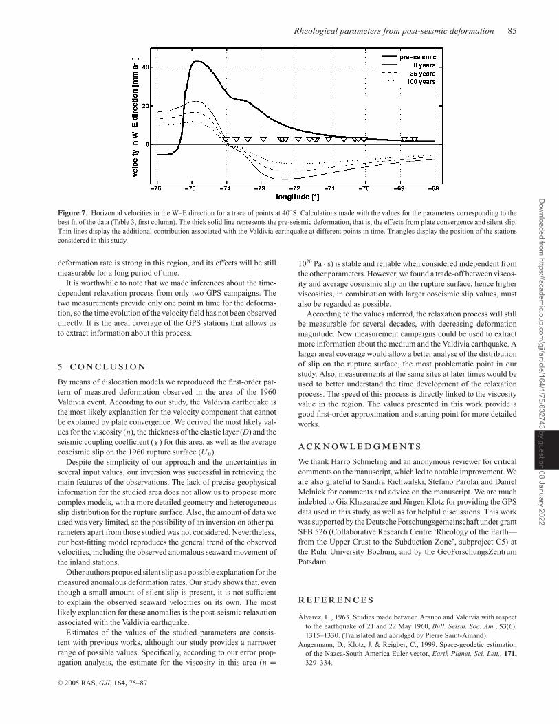
Fig. 7 shows the W–E deformation rate for a trace of points at40◦S for the best-fitting model, both before the earthquake and theadditional contribution of the event at different moments after theValdivia earthquake. From Figs 6 and 7 it follows that stations inthe range between 70 to 73◦W will be the most adequate to furtheranalyse the relaxation process, since the time dependence of the

C© 2005 RAS, GJI, 164, 75–87

Dow




Figure 7. Horizontal velocities in the W–E direction for a trace of points at 40◦S. Calculations made with the values for the parameters corresponding to thebest fit of the data (Table 3, first column). The thick solid line represents the pre-seismic deformation, that is, the effects from plate convergence and silent slip.Thin lines display the additional contribution associated with the Valdivia earthquake at different points in time. Triangles display the position of the stationsconsidered in this study.

deformation rate is strong in this region, and its effects will be stillmeasurable for a long period of time.

It is worthwhile to note that we made inferences about the time-dependent relaxation process from only two GPS campaigns. Thetwo measurements provide only one point in time for the deforma-tion, so the time evolution of the velocity field has not been observeddirectly. It is the areal coverage of the GPS stations that allows usto extract information about this process.

5 C O N C L U S I O N

By means of dislocation models we reproduced the first-order pat-tern of measured deformation observed in the area of the 1960Valdivia event. According to our study, the Valdivia earthquake isthe most likely explanation for the velocity component that cannotbe explained by plate convergence. We derived the most likely val-ues for the viscosity (η), the thickness of the elastic layer (D) and theseismic coupling coefficient (χ ) for this area, as well as the averagecoseismic slip on the 1960 rupture surface (U 0).

Despite the simplicity of our approach and the uncertainties inseveral input values, our inversion was successful in retrieving themain features of the observations. The lack of precise geophysicalinformation for the studied area does not allow us to propose morecomplex models, with a more detailed geometry and heterogeneousslip distribution for the rupture surface. Also, the amount of data weused was very limited, so the possibility of an inversion on other pa-rameters apart from those studied was not considered. Nevertheless,our best-fitting model reproduces the general trend of the observedvelocities, including the observed anomalous seaward movement ofthe inland stations.

Other authors proposed silent slip as a possible explanation for themeasured anomalous deformation rates. Our study shows that, eventhough a small amount of silent slip is present, it is not sufficientto explain the observed seaward velocities on its own. The mostlikely explanation for these anomalies is the post-seismic relaxationassociated with the Valdivia earthquake.

Estimates of the values of the studied parameters are consis-tent with previous works, although our study provides a narrowerrange of possible values. Specifically, according to our error prop-agation analysis, the estimate for the viscosity in this area (η =

1020 Pa · s) is stable and reliable when considered independent fromthe other parameters. However, we found a trade-off between viscos-ity and average coseismic slip on the rupture surface, hence higherviscosities, in combination with larger coseismic slip values, mustalso be regarded as possible.

According to the values inferred, the relaxation process will stillbe measurable for several decades, with decreasing deformationmagnitude. New measurement campaigns could be used to extractmore information about the medium and the Valdivia earthquake. Alarger areal coverage would allow a better analyse of the distributionof slip on the rupture surface, the most problematic point in ourstudy. Also, measurements at the same sites at later times would beused to better understand the time development of the relaxationprocess. The speed of this process is directly linked to the viscosityvalue in the region. The values presented in this work provide agood first-order approximation and starting point for more detailedworks.

A C K N O W L E D G M E N T S

We thank Harro Schmeling and an anonymous reviewer for criticalcomments on the manuscript, which led to notable improvement. Weare also grateful to Sandra Richwalski, Stefano Parolai and DanielMelnick for comments and advice on the manuscript. We are muchindebted to Gia Khazaradze and Jurgen Klotz for providing the GPSdata used in this study, as well as for helpful discussions. This workwas supported by the Deutsche Forschungsgemeinschaft under grantSFB 526 (Collaborative Research Centre ‘Rheology of the Earth—from the Upper Crust to the Subduction Zone’, subproject C5) atthe Ruhr University Bochum, and by the GeoForschungsZentrumPotsdam.

R E F E R E N C E S

Alvarez, L., 1963. Studies made between Arauco and Valdivia with respectto the earthquake of 21 and 22 May 1960, Bull. Seism. Soc. Am., 53(6),1315–1330. (Translated and abridged by Pierre Saint-Amand).

Angermann, D., Klotz, J. & Reigber, C., 1999. Space-geodetic estimationof the Nazca-South America Euler vector, Earth Planet. Sci. Lett., 171,329–334.

C© 2005 RAS, GJI, 164, 75–87

Dow




Araujo, M. & Suarez, G., 1994. Geometry and state of stress of the sub-ducted Nazca plate beneath central Chile and Argentina: evidence fromteleseismic data, Geophys. J. Int., 116, 283–303.

Askew, B.L. & Algermissen, S.T., 1985. Catalog of earthquakes for SouthAmerica: hypocenter and intensity data, Vol. 4, 6 and 7a, b and c. OnlineData Set available from USGS National Earthquake Information Center:http://wwwneic.cr.usgs.gov/neis/epic/epic.html.

Barrientos, S.E. & Ward, S.N., 1990. The 1960 Chile earthquake: inversionfor slip distribution from surface deformation, Geophys. J. Int., 103, 589–598.

Barrientos, S.E., Plafker, G. & Lorca, E., 1992. Postseismic coastal uplift inSouthern Chile, Geophys. Res. Lett., 19, 701–704.

Benioff, H., Press, F. & Smith, S., 1961. Excitation of the free oscillationsof the Earth by earthquakes, J. geophys. Res., 66, 605–619.

Bohm, M., Luth, S., Echtler, H., Asch, G., Bataille, K., Bruhn, C., Rietbrock,A. & Wigger, P., 2002. The Southern Andes between 36◦ and 40◦S latitude:seismicity and average seismic velocities, Tectonophysics, 356, 275–289.

Brown, L., Reilinger, R., Holdhal, S.R. & Balazs, E.I., 1977. Postseismiccrustal uplift near Anchorage, Alaska, J. geophys. Res., 82, 3369–3378.

Cahill, T. & Isacks, B.L., 1992. Seismicity and shape of the subducted Nazcaplate, J. geophys. Res., 97(B12), 17 503–17 529.

Chase, C.G., 1978. Plate kinematics: the Americas, East Africa, and the restof the world, Earth planet. Sci. Lett., 37, 355–368.

Christensen, R.M., 1982. Theory of Viscoelasticity. An introduction, 2nd edn,Academic Press, New York.

Cifuentes, I.L., 1989. The 1960 Chilean Earthquakes, J. geophys. Res., 94,665–680.

Cohen, S.C., 1980a. Postseismic viscoelastic surface deformation and stress- 1. Theoretical considerations, displacement and strain calculations,J. geophys. Res., 85, 3131–3150.

Cohen, S.C., 1980b. Postseismic viscoelastic deformation and stress—2.Stress theory and computation; dependence of displacement, strain, andstress on fault parameters, J. geophys. Res., 85, 3151–3158.

Cohen, S.C., 1982. A multilayer model of time-dependent deformation fol-lowing an earthquake on a strike-slip fault, J. geophys. Res., 87(B7), 5409–5421.

Cohen, S.C., 1994. Evaluation of the importance of model features forcyclic deformation due to dip-slip faulting, Geophys. J. Int., 119, 831–841.

Conrad, C.P., Bilek, S. & Lithgow-Bertelloni, C., 2004. Great earthquakesand slab pull: interaction between seismic coupling and plate-slab cou-pling, Earth Planet. Sci. Lett., 218, 109–122.

DeMets, C., Gordon, R.G., Argus, D.F. & Stein, S., 1990. Current platemotions, Geophys. J. Int., 101, 425–478.

DeMets, C., Gorden, R.G., Argus, D.F. & Stein, S., 1994. Effect of recentrevisions to the geomagnetic reversal timescale on estimates of currentplate motion, Geophys. Res. Lett., 21, 2191–2194.

Fernandez, J., Yu, T.-T. & Rundle, J.B., 1996. Horizontal viscoelastic-gravitational displacement due to a rectangular dipping thrust fault in alayered earth model, J. geophys. Res., 101, 13 581–513 594. (Correction:JGR: 103, B12, 30, 283–286, 1998).

Fernandez, J. & Rundle, J.B., 2004. Postseismic viscoelastic-gravitationalhalf space computations: problems and solutions, Geophys. Res. Lett., 31,L07608, doi:10.1029/2004GL019654.

Fitch, T.J. & Scholz, C.H., 1971. Mechanism of underthrusting in southwestJapan: a model of convergent plate interaction, J. geophys. Res., 76, 7260–7292.

Freed, A.M. & Burgmann, R., 2004. Evidence of power-law flow in theMojave desert mantle, Nature, 430(6999), 548–551.

Freymueller, J.T., Cohen, S.C. & Fletcher, H.J., 2000. Spatial variations inpresent-day deformation, Kenai Peninsula, Alaska, and their implications,J. geophys. Res., 105, 8079–8101.

Hu, Y., Wang, K., He, J., Klotz, J. & Khazaradze, G., 2004. 3-D viscoelasticfinite element model for postseismic deformation of the great 1960 Chileearthquake, J. geophys. Res., 109, B12403, doi:10.1029/2004JB003163.

James, T.S., Clague, J.J., Wang, K. & Hutchinson, I., 2000. Postglacial re-bound at the northern Cascadia subduction zone, Quaternary ScienceReviews, 19, 1527–1541.

Jordan, T.E., Isacks, B.L., Allmendiger, R.W., Brewer, J.A., Ramos, V.A.& Ando, C.J., 1982. Andean tectonics related to geometry of subductedNazca plate, Geol. Study of Am. Bull., 94, 341–361.

Kanamori, H., 1977. The energy release in great earthquakes, J. geophys.Res., 82(20), 2981–2987.

Kanamori, H. & Cipar, J.J., 1974. Focal process of the great Chilean earth-quake May 22, 1960, Phys. Earth Planet. Int., 9, 128–136.

Kasahara, K., 1975. Aseismic faulting following the 1973 Nemuro-Okiearthquake, Hokkaido, Japan (a possibility), Pure Appl. Geophys., 113,127–139.

Khazaradze, G. & Klotz, J., 2003. Short- and long-term effects of GPS mea-sured crustal deformation rates along the south central Andes, J. geophys.Res., 108(B6), ETG 5-1 to ETG 5-15, 2289, doi:10.1029/2002JB001879.

Khazaradze, G., Wang, K., Klotz, J., Hu, Y. & He, J., 2002. Prolongedpost-seismic deformation of the 1960 great Chile earthquake and im-plications for mantle rheology, Geophys. Res. Lett., 29(22), 7–1 to 7–4,doi:10.1029/2002GL015986.

Klotz, J., Khazaradze, G., Angermann, D., Reigber, C., Perdomo, R. &Cifuentes, O., 2001. Earthquake cycle dominates contemporary crustaldeformation in Central and Southern Andes, Earth Planet. Sci. Lett.,193(3–4), 437–446.

Krawczyk, C. & the SPOC team, 2003. Amphibious seismic survey imagesplate interface at 1960 Chile earthquake, EOS, Trans., 84(32), 301–312.

Lambeck, K., 1980. The Earth’s variable rotation: geophysical causes andconsequences, Cambridge University Press, London.

Linde, A.T. & Silver, P.G., 1989. Elevation changes and the great 1960earthquake: support for aseismic slip, Geophys. Res. Lett., 16, 1305–1308.

Lorenzo Martın, F., Wang, R. & Roth, F., 2002. The effect of input parameterson visco-elastic models of crustal deformation, Fısica de la Tierra, 14,33–54.

Luth, S., Wigger, P. & the ISSA Research Group, 2003. A crustal model along39◦S from a seismic refraction profile- ISSA 2000, Rev. geol. Chile, 30(1),83–101.

Nason, R. & Weertman, J., 1973. A dislocation theory analysis of fault creepevents, J. geophys. Res., 78, 7745–7751.

Nishenko, S.P., 1985. Seismic potential for large and great earthquakes alongthe Chilean and southern Peruvian margins of South America: a quanti-tative reappraisal, J. geophys. Res., 90(B5), 3589–3615.

Norabuena, E., Leffler-Griffin, L., Mao, A., Dixon, T., Stein, S., Sacks, I.S.,Ocola, L. & Ellis, M., 1998. Space geodetic observations of Nazca-SouthAmerica convergence across the central Andes, Science, 279(22), 358–362.

Norabuena, E., Dixon, T.H., Stein, S. & Harrison, C.G.A., 1999. Deceler-ating Nazca-South America and Nazca-Pacific plate motions, Geophys.Res. Lett., 26(22), 3405–3408.

Nur, A. & Mavko, G., 1974. Postseismic viscoelastic rebound, Science, 181,204–206.

Oleskevich, D.A., Hyndman, R.D. & Wang, K., 1999. The updip and downdiplimits to great subduction earthquakes: thermal and structural modelsof Cascadia, south Alaska, SW Japan, and Chile, J. geophys. Res., B7,14 965–14 991.

Piersanti, A., 1999. Postseismic deformation in Chile: constraints on theasthenospheric viscosity, Geophys. Res. Lett., 26(20), 3157–3160.

Plafker, G., 1972. Alaskan earthquake of 1964 and Chilean earthquake of1960: implications for arc tectonics, J. geophys. Res., 77, 901–925.

Plafker, G. & Savage, J.C., 1970. Mechanism of the Chilean earthquakes ofMay 21 and 22, 1960, Geol. Soc. Am. Bull., 81, 1001–1030.

Pollitz, F.F., Burgmann, R. & Segall, P., 1998. Joint estimation of afterslip rateand postseismic relaxation following the 1989 Loma Prieta earthquake, J.geophys. Res. B: Solid Earth, 103(B11), 26 975–26 992.

Pollitz, F.F., Wicks, C. & Thatcher, W., 2001. Mantle flow beneath a con-tinental strike-slip fault: postseismic deformation after the 1999 HectorMine earthquake, Science, 293(5536), 1814–1818.

Press, F., Ben-Menahem, A. & Toksoz, M.N., 1961. Experimental determi-nation of earthquake fault length and rupture velocity, J. geophys. Res.,66, 3471–3485.

Rundle, J.B., 1982. Viscoelastic-gravitational deformation by a rectangularthrust fault in a layered Earth, J. geophys. Res., 87, 7787–7796.

C© 2005 RAS, GJI, 164, 75–87

Dow




Savage, J.C. & Plafker, G., 1991. Tide gage measurements of uplift alongthe south coast of Alaska, J. geophys. Res., 96, 4325–4335.

Scholz, C.H. & Campos, J., 1995. On the mechanism of seismic decouplingand back arc spreading at subduction zones, J. geophys. Res., 100, 22 103–22 115.

Smith, W.H.F. & Sandwell, D.T., 1997. Global seafloor topography fromsatellite altimetry and ship depth soundings, Science, 277, 1957–1962.

Somoza, R., 1998. Updated Nazca (Farallon)-South America relative mo-tions during the last 40 My: implications for mountain building in thecentral Andean region, Journal of South American Earth Sciences, 11(3),211–215.

Talley, H.C. & Cloud, W.K., 1962. United States Earthquakes 1960, U.S.Department of Commerce, Coast and Geodetic Survey—Washington,Washington, D.C.

Thatcher, W. & Rundle, J.B., 1984. A viscoelastic coupling model for thecyclic deformation due to periodical repeated earthquakes at subductionzones, J. geophys. Res., 89, 7631–7640.

Tichelaar, B.W. & Ruff, L.J., 1991. Seismic coupling along the Chileansubduction zone, J. geophys. Res., 96(B7), 11 997–12 022.

Uyeda, S., 1982. Subduction zones, an introduction to comparative subduc-tology, Tectonophysics, 81, 133–159.

Vermeersen, L.L. A., Sabadini, R., Devoti, R., Luceri, V., Rutigliano, P. &Sciarretta, C., 1998. Mantle viscosity inferences from joint inversion of

pleistocene deglaciation-induced changes in geopotential with a new SLRanalysis and polar wander, Geophys. Res. Lett., 25(23), 4261–4264.

Wang, R., 1999. A simple orthonormalization method for the stable andefficient computation of Green’s functions, Bull. Seism. Soc. Am., 89,733–741.

Wang, R., 2005. On the singularity problem of the elastic-gravitational dis-location theory applied to plane-earth models, Geophys. Res. Lett., 32,L06307, doi:10.1029/2003GL019358.

Wang, R., Lorenzo Martın, F. & Roth, F., 2003. Computation of deforma-tion induced by earthquakes in a multi-layered elastic crust - FORTRANprograms EDGRN/EDCMP, Computers and Geosciences, 29(2), 195–207.

Wang, R., Lorenzo-Martın, F. & Roth, F., 2005. A semi-analytical soft-ware PSGRN/PSCMP for calculating co- and post-seismic deformationon a layered viscoelastic-gravitational half-space, Computers and Geo-sciences, in press.

Yu, T.-T., Rundle, J.B. & Fernandez, J., 1996. Surface deformation due toa strike-slip fault in an elastic gravitational layer overlying a viscoelasticgravitational half-space, J. geophys. Res., 101, 3199–3214. (Correction:JGR, 104, B7, 15,313–5, 1999).

Zweck, C., Freymueller, J.T. & Cohen, S.C., 2002. 3-D elastic dislocationmodeling of the postseismic response to the 1964 Alaska earthquake,J. geophys. Res., 107(B4), doi:10.1029/2001JB000409.

C© 2005 RAS, GJI, 164, 75–87

Dow



Documents

Inversion for rheological parameters from post-seismic surface