INVERSE TIME-HARMONIC ELECTROMAGNETIC SCATTERING …

INVERSE TIME-HARMONIC ELECTROMAGNETIC SCATTERING FROMCOATED POLYHEDRAL SCATTERERS WITH A SINGLE FAR-FIELD

PATTERN

GUANG-HUI HU†, MANMOHAN VASHISTH‡ AND JIAQING YANG∗

Abstract. It is proved that a convex polyhedral scatterer of impedance type can be uniquelydetermined by the electric far-field pattern of a non-vanishing incident field. The incoming wave isallowed to be an electromagnetic plane wave, a vector Herglotz wave function or a point source waveincited by some magnetic dipole. Our proof relies on the reflection principle for Maxwell’s equationswith the impedance (or Leontovich) boundary condition enforcing on a hyper-plane. We prove thatit is impossible to analytically extend the total field across any vertex of the scatterer. This leadsto a data-driven inversion scheme for imaging an arbitrary convex polyhedron.

Keywords: Uniqueness, inverse electromagnetic scattering, polyhedral scatterer, reflection prin-ciple, impedance boundary condition, single incident wave, data-driven scheme.

Mathematics subject classification 2010: 35R30,78A46, 35J15.

1. Introduction and Main Result

The propagation of time-harmonic electromagnetic waves in a homogeneous isotropic medium inR3 is modelled by the Maxwell’s equations

∇× E(x)− ikH(x) = 0, ∇×H(x) + ikE(x) = 0 for x ∈ R3,(1.1)

where E and H represent the electric and magnetic fields respectively and k > 0 is known asthe wave number. Let Ein and H in satisfying Equation (1.1) denote the incident electric andmagnetic fields respectively. Consider the scattering of given incoming waves Ein and H in from aconvex polyhedral scatterer D ⊂ R3 coated by a thin dielectric layer, which can be modelled bythe impedance (or Leontovich) boundary value problem of the Maxwell’s equations (1.1) in R3\D.Then the total fields E = Ein+Esc, H = H in+Hsc, where Esc and Hsc denote the scattered fields,are governed by the following set of Equations (1.2)-(1.5):

∇× E − ikH = 0, ∇×H + ikE = 0 in R3\D,(1.2)

E = Ein + Esc, H = H in +Hsc in R3\D,(1.3)

lim|x|→∞

(Hsc × x− |x|Esc) = 0,(1.4)

ν × (∇× E) + iλν × (ν × E) = 0 on ∂D,(1.5)

where ν denotes the outward unit normal to ∂D and the impedance coefficient λ > 0 is supposedto be a constant. Equation (1.4) is known as the Silver-Muller radiation condition and is uniformin all directions x := x/|x|. For the existence and uniqueness of the solution (E,H) to the forwardsystem (1.2)-(1.5), we refer to [10] when ∂D is C2-smooth and to [4, 6] when ∂D is Lipschitz withconnected exterior. Moreover, the Silver-Muller radiation condition (1.4) ensures that scattered

1

2 HU, VASHISTH AND YANG

fields Esc and Hsc satisfy the following asymptotic behaviour (see [10])

Esc(x) =eik|x|

|x|

(E∞ (x) +O

(1

|x|

)), as |x| → ∞,(1.6)

Hsc(x) =eik|x|

|x|

(H∞ (x) +O

(1

|x|

)), as |x| → ∞(1.7)

where the vector fields E∞ and H∞ defined on the unit sphere S2, are called the electric andmagnetic far-field patterns of the scattered waves Esc and Hsc, respectively. It is well known thatE∞ and H∞ are analytic functions with respect to the observation direction x ∈ S2 and satisfy thefollowing relations

H∞ = ν × E∞, ν · E∞ = ν ·H∞ = 0,(1.8)

where ν denotes the unit normal vector to the unit sphere S2.Given the incoming wave (Ein, H in) and the scatterer D ⊂ R3, the direct problem arising from

electromagnetic scattering is to find the scattered fields (Esc, Hsc) and their far-field patterns. Theinverse problem to be considered in this paper consists of determining the location and shape of Dfrom knowledge of the far-field patterns (E∞, H∞). We assume that the incident fields Ein and H in

are non-vanishing vector fields which are solutions to the Maxwell’s equations (1.1) in a neighboringarea of the obstacle D. For instance one can take the incident fields Ein and H in to be one amongthe following:

(1) Plane waves:

Ein(x, d, p) = peikx·d, H in(x, d, p) = (d× p)eikx·d(1.9)

where d ∈ S2 is known as the incident direction and p ∈ S2 with p ⊥ d is known as thepolarization direction.

(2) Point source waves:

Ein = ∇× (Φ(x, y)~a) , H in(x) =1

ik∇× Ein(x), x 6= y,(1.10)

where ~a is a constant vector and Φ(x, y) := 14π

eik|x−y|

|x−y| , x 6= y is the fundamental solution to

∆ + k2 in R3. (Ein, H in) given by (1.10) represent the electromagnetic field generated by amagnetic dipole located at y and they solve the Maxwell’s equations (1.1) for x 6= y.

(3) Electromagnetic Herglotz pairs:

Ein(x) =

∫S2

eikx·da(d)ds(d), H in(x) =1

ik∇× Ein(x), x ∈ R3,(1.11)

where the square integrable tangential field a ∈ L2t (S2)3 is known as the Herglotz kernel of

Ein and H in.

The present article is concerned with a uniqueness result of determining the convex polyhedralscatterer D appearing in the system of Equations (1.2)-(1.5) from the knowledge of a single electricfar-field pattern E∞(x) measured over all observation directions x ∈ S2. We mention that in caseof plane wave incidence, the incident direction d ∈ S2, the polarization direction p ∈ S2 and thewave number k > 0 are all fixed.

We state our main result as follows:

INVERSE ELECTROMAGNETIC SCATTERING 3

Theorem 1.1. Let D1 and D2 be two convex polyhedral scatterers of impedance type. Given anincident field (Ein, H in) as mentioned above, we denote by E∞j (j = 1, 2) the electric far-fieldpatterns of the scattering problem (1.2)-(1.5) when D = Dj. Then the relation

E∞1 (x) = E∞2 (x) for all x ∈ S2(1.12)

implies that D1 = D2.

It is widely open how to uniquely determine the shape of a general impenetrable/penetrablescatterer using a single far-field pattern. As in the acoustic case [1,2,7,27], quite limited progress hasalso been made in inverse time-harmonic electromagnetic scattering. To the best of our knowledge,global uniqueness with a single measurement data is proved only for perfectly conducting obstacleswith restrictive geometric shapes such like balls [26] and convex polyhedrons [10, Chapter 7.1].Without the convexity condition, it was shown in [29] that a general perfect polyhedral conductor(the closure of which may contain screens) can be uniquely determined by the far-field pattern forplane wave incidence with one direction and two polarizations. We shall prove Theorem 1.1 by usingthe reflection principle for Maxwell’s equations with the impedance boundary condition enforcing ona hyper-plane. It seems that such a reflection principle has not been studied in prior works, althoughthe corresponding principle under the perfectly conducting boundary condition is well known inoptics (see e.g. [29]). Theorem 1.1 carries over to perfectly conducting polyhedrons with a singlefar-field pattern (see Corollary 4.5), and thus improves the acoustic uniqueness result for impedancescatterers [8] where two incident directions were used. It is also worth mentioning other works in theliterature related to reflection principles for the Helmholtz and Navier equations together with theirapplications to uniqueness in inverse acoustic and elastic scattering [1, 7, 9, 13–15, 28]. We believethat the reflection principle, as a special case of unique continuation, provides a powerful tool forgaining new insights into inverse scattering problems. More remarks concerning our uniquenessproof will be concluded in Section 4.2.

In the second part of this paper, we shall propose a novel non-iterative scheme for imaging anarbitrary convex-polyhedron from a single electric far-field pattern. The Linear Sampling Methodin inverse electromagnetic scattering [3–6] was earlier studied with infinite number of plane waves ata fixed energy. We are mostly motivated by the uniqueness proof of Theorem 1.1 (see also Corollary4.4) and the one-wave factorization method in inverse elastic and acoustic scattering [15, 18]. Theproposed scheme is essentially a domain-defined sampling approach, requiring no forward solvers.Promising features of our imaging scheme are summarised as follows.

(i) It requires lower computational cost and only a single measurement data. The proposeddomain-defined indicator function involves only inner product calculations. Since the number ofsampling variables is comparable with the original Linear Sampling Method and FactorizationMethod ( [3, 10, 22]), the computational cost is not heavier than the aforementioned pointwise-defined sampling methods. (ii) It can be interpreted as a data-driven approach, because it relies onmeasurement data corresponding to a priori given scatterers (which are also called test domains inthe literature or samples in the terminology of learning theory and data science). There is a varietyof choices on the shape and physical properties of these samples, giving arise to quite “rich”a priorisample data in addition to the measurement data of the unknown target. In this paper, we chooseperfectly conducting balls (or impedance balls) as test domains, because the spectra of the resultingfar-field operator admit explicit representations. However, these test domains can also be chosenas any other convex penetrable and impenetrable scatterers, provided the classical factorizationscheme for imaging this test domain can be verified using all incident and polarization directions.We refer to [23] for the Factorization Method applied to inverse electromagnetic medium scattering


problems. (iii) It provides a necessary and sufficient criterion for imaging convex polyhedrons (seeTheorem 5.2) with a single incoming wave. We prove that the wave fields cannot be analytic aroundany vertex of D (see Corollary 4.4), excluding the possibility of analytical extension across a vertex.Some other domain-defined sampling approaches such as the range test approach [24,25] and the one-wave no-response test [31, 32] usually pre-assume such extensions, leading to a sufficient conditionfor imaging general targets. Our approach is closest to the No Response Test for reconstructingperfectly conducting polyhedral scatterers with a few incident plane waves [33] and is comparablewith the one-wave enclosure method by Ikehata [20,21] for capturing singular points of ∂D. Detaileddiscussions on the issue of analytic continuation tests can be found in the monograph [36, Chapter 15](see also [17]). If ∂D contains no singular points, only partial information of D can be numericallyrecovered; see [30] where the linear sampling method with a single far-field pattern was tested.

We organize the article as follows. In §2 we prove Theorem 1.1 when the incident fields aregiven by (1.9). In §3 we state and prove the reflection principle for Maxwell’s equations with theimpedance boundary condition on a hyper-plane in R3 (see Theorem 3.1). Using this reflectionprinciple we prove in §4.1 the main uniqueness results for electromagnetic Herglotz waves and pointsource waves. The data-driven reconstruction scheme will be described in §5.

2. Uniqueness with a Single Plane Wave

In this section, we prove Theorem 1.1, when the incident fields (Ein, H in) are given by

Ein(x, d, p) = peikx·d, H in(x, d, p) = (d× p)eikx·d

where d, p ∈ S2 satisfying p ⊥ d and k > 0 are all fixed. Now recall from Equation (1.12) thatE∞1 (x) = E∞2 (x) for all x ∈ S2. Using the Rellich’s lemma (see [10]) we get

E1 = E2 and H1 = H2 in R3 \(D1 ∪D2

).

Assuming thatD1 6= D2, we shall prove the uniqueness by deriving a contradiction. By the convexityof D1 and D2, we may assume that there exists a vertex O of ∂D1 and a neighborhood VO of O suchthat VO ∩ D2 = ∅. Next using the impedance boundary condition of E1 on ∂D1 and E1 = E2 inR3 \

(D1 ∪D2

), we have that ν× (∇× E2) + iλν× (ν × E2) = 0 on VO ∩∂D1. Since D1 is a convex

polyhedron, there exists m (m ≥ 3) convex polygonal faces Λj (j = 1, 2 · · ·m) of ∂D1 whose closuremeet at O and which can be analytically extended to infinity in R3\D2; for example, see Figure

1 on page 12, where m = 4 (left) and m = 3 (right). Denote by Π ⊇ Λj the maximum extensionof Λj in R3\D2. Using the real-analyticity of E2 in R3\D2 together with the fact that λ > 0 is a

constant, we conclude that E2 satisfies the impedance boundary condition on Πj. Recalling (1.4)and (1.6), we have lim

|x|→∞|∇ × Esc

2 | = 0, lim|x|→∞

|Esc2 | = 0. Hence,

ν ×(∇× Ein

)+ iλν ×

(ν × Ein

)= 0 on Πj, j = 1, 2, · · ·m.(2.1)

By Equation (1.9), it then follows that

ikν × (d× p) + iλν × (ν × p) = 0,(2.2)

holds for any outward unit normal ν to Πj. Without loss of generality, we suppose that p = e1,d × p = e2, ν = c1e1 + c2e2 + c3e3 with c2

1 + c22 + c2

3 = 1, where ej ∈ S2 (j = 1, 2, 3) denotes theCartesian coordinates in R3. By (2.2), simple calculations show that

−(kc3 + λ(c2

2 + c23))e1 + λc1c2e2 + (kc1 + λc1c3) e3 = 0.


This gives us the equations of cj,

kc3 = −λ(c2

2 + c23

), λc1c2 = 0, kc1 = −λc1c3,

which have the following solutions for ν = (c1, c2, c3) ∈ S2:

ν = (0, 0,−1), if k = λ;

ν =(±√

1− (k/λ)2, 0,−k/λ), if k < λ;

ν =(

0,±√

1− (λ/k)2,−λ/k), if k > λ.

Hence, the relation (2.2) cannot hold for three linearly independent unit normal vectors ν. Thiscontradiction implies that D1 = D2.

Remark 2.1. The above uniqueness proof with a single plane wave cannot be applied to the Helmholtzequation in two dimensions under the impedance boundary condition ∂νu+ iλu = 0. In 2D case, wededuce a corresponding relation kν · d + λ = 0, which holds for only two linearly independent unitnormal vectors if D1 6= D2. However, this cannot lead to a contradiction when k > λ. It was provedin [8] that the far-field patterns of two incident directions uniquely determine a convex polygonalobstacle of impedance type.

Since the above proof relies on the form of electromagnetic plane waves therefore it is not appli-cable to the incident fields given by electromagnetic point source waves and vector Herglotz wavefunctions. For these kind of incident fields, we shall apply the reflection principle for Maxwell’sequations to prove Theorem 1.1; see Sections 3 and subsection 4.1 below.

3. Reflection Principle for Maxwell’s Equations

Let Ω ⊆ R3 be an open connected set which is symmetric with respect to a plane Π in R3 and wedefine by γ := Ω∩Π. Denote by Ω+ and Ω− the two symmetric parts of Ω which are divided by Π andby RΠ the reflection operator about Π, that is, if x ∈ Ω± then RΠx ∈ Ω∓ for x = (x1, x2, x3) ∈ Ω.Throughout this article, Ω will be assumed in such a way that any line segment with end points inΩ and intersected with Π by the angle π/2 lies completely in Ω. In other words, the projection ofany line segment in Ω onto the hyperplane Π is a subset of γ. This geometrical condition was alsoused in [12] where the reflection principle for the Helmholtz equation with the impedance boundarycondition was verified in Rn (n ≥ 2). Now consider the time-harmonic Maxwell’s equations withthe impedance boundary condition by

∇× E − ikH = 0, ∇×H + ikE = 0, in Ω+,(3.1)

ν × (∇× E) + iλν × (ν × E) = 0, on γ ⊂ Π.(3.2)

It is well known from (Theorem 6.4 in [10]) that a solution (E,H) of Equation (3.1) satisfies thevectorial Helmholtz equations with the divergence-free condition:

∆E + k2E = 0, ∆H + k2H = 0, ∇ · E = ∇ ·H = 0.(3.3)

Since Equations (3.3) and (3.1) are rotational invariant, without loss of generality we can assumethat the plane Π mentioned above coincides with the ox1x2-plane, i.e., Π = (x1, x2, x3) ∈ R3 :x3 = 0. Consequently, we have ν = e3 := (0, 0, 1)T and RΠx = (x1, x2,−x3). In this section,we study the reflection principle for solutions to the Maxwell’s equation satisfying the impedanceboundary condition on γ. Our aim is to extend the solution (E,H) of Equation (3.1) from Ω+ toΩ− by an analytical formula. The reflection principle is stated as follows.


Theorem 3.1. Let Π := (x′, x3) ∈ R3 : x3 = 0 with x′ := (x1, x2), γ ⊂ Ω ∩ Π and Ω± :=(x1, x2, x3) ∈ Ω : ±x3 > 0. Assume that (E,H) satisfies Equation (3.1) with the boundarycondition (3.2). Then (E,H) can be analytically extended to Ω− as a solution to (3.1). Moreover,

the extended electric field E :=(E1, E2, E3

)Tis given explicitly by

E(x′, x3) =

E(x), if x ∈ Ω+ ∪ γDE(x′,−x3), if x ∈ Ω−

(3.4)

where the operator DE := ((DE)1, (DE)2, (DE)3)T is defined by

(DE)3(x) := E3(x′, x3)− 2k2

iλ

x3∫0

ek2

iλ(s−x3)E3(x′, s)ds for x ∈ Ω+,(3.5)

(DE)j(x′, x3) := Ej(x

′, x3) + 2iλ

x3∫0

e−iλ(s−x3)Ej(x′, s)ds(3.6)

+2λ2

k2 − λ2

x3∫0

e−iλ(s−x3)∂jE3(x′, s)ds− 2k2

k2 − λ2

x3∫0

ek2

iλ(s−x3)∂jE3(x′, s)ds

for j = 1, 2 and x ∈ Ω+.

Obviously, the extension operator (DE)3 only relies on E3 in Ω+, whereas (DE)j (j = 1, 2)depends on both Ej and E3. The formula given by (3.4) is a ‘non-point-to-point’ reflection formulawhich is in contrast with the ‘point-to-point’ reflection formula for the Maxwell’s equations withthe Dirichlet boundary condition (see [29]). As λ→∞, the impedance boundary condition will bereduced to the Dirichlet boundary condition ν×E = 0 on Π. It is easy to observe that (DE)3 → E3

and by applying integration by part that (DE)j → −Ej for j = 1, 2 as λ tends to infinity. Hence, the

reflection formula (3.4) becomes E(x) = −RΠE(RΠx) for x ∈ Ω, which is valid for any symmetricdomain with respect to Π = x : x3 = 0. Before going to the proof of Theorem 3.1, we first statethe reflection principle for the Helmholtz equation with an impedance boundary condition. Theresult in the following Lemma 3.2 has already been proved in [12].

Lemma 3.2. [12] Let Ω,Π,γ and Ω± be defined as in Theorem 3.1. If u is a solution to theboundary value problem of the Helmholtz equation

(3.7) ∆u+ k2u = 0 in Ω+, ∂νu+ iλu = 0 on γ,

then u can be extended from Ω+ to Ω as a solution to the Helmholtz equation, with the extendedsolution u given by the formula u := u in Ω+ ∪ γ and

(3.8) u(x) := u(x1, x2,−x3) + 2iλe−iλx3−x3∫0

e−iλsu(x1, x2, s)ds in Ω−.

Our proof of Theorem 3.1 is essentially motivated by the proof of Lemma 3.2.

3.1. Proof of Theorem 3.1. From Equation (3.1), we deduce that E is a solution to

∇× (∇× E)− k2E = 0 in Ω+, e3 × (∇× E) + iλe3 × (e3 × E) = 0 on γ.(3.9)


Define the vector function F and the scalar function V by

F := e3 × (∇× E) + iλe3 × (e3 × E) =: (F1, F2, 0)T in Ω+,

F1 = ∂1E3 − ∂3E1 − iλE1, F2 = ∂2E3 − ∂3E2 − iλE2,(3.10)

V :=∂1F1 + ∂2F2

iλ=∂2

1E3 − ∂231E1 − iλ∂1E1 + ∂2

2E3 − ∂232E2 − iλ∂2E2

iλ.

Now using ∆E + k2E = 0 and ∇ · E = 0 in Ω+, we have

V =−∂2

3E3 − k2E3 − ∂3 (∂1E1 + ∂2E2)− iλ (∂1E1 + ∂2E2)

iλ= ∂3E3 −

k2

iλE3.

Since F1 = F2 = 0 on γ ⊆ x ∈ R3 : x3 = 0, we get ∂1F1 = ∂2F2 = 0 on γ and thus

∆E3 + k2E3 = 0 in Ω+, ∂3E3 − k2/(iλ) E3 = 0 on γ.(3.11)

Applying Lemma 3.2, we can extend E3 from Ω+ to Ω by E3 := E3 in Ω+ ∪ γ and

E3(x) := E3(x′,−x3)− 2k2

iλek2

iλx3

−x3∫0

ek2

iλsE3(x′, s)ds in Ω−,

which gives the extension formula for E3. To find the extension formula for Ej (j = 1, 2), we observethat Fj (j = 1, 2) given by (3.10) satisfy the Helmholtz equation with the Dirichlet boundarycondition,

∆Fj + k2Fj = 0 in Ω+, Fj = 0 on γ.

Applying the reflection principle with the Dirichlet boundary condition (see [12]), we can extend Fjthrough Fj := Fj in Ω+ ∪ γ and Fj(x) := −Fj(x′,−x3) in Ω−. As done for the Helmholtz equation,we will derive the extension formula for Ej for j = 1, 2 by considering the boundary value problemof the ordinary differential equation (cf. (3.10))

∂3Ej + iλEj − ∂jE3 = −Fj in Ω, Ej = Ej on γ,

where Ej (j = 1, 2) denote the extended functions. Multiplying the above equation by eiλx3 andintegrating between 0 to x3, we have

x3∫0

eiλs(∂sEj(x

′, s) + iλEj(x′, s))

ds−x3∫

0

eiλs∂jE3(x′, s)ds = −x3∫

0

eiλsFj(x′, s)ds,

which gives us

Ej(x) = e−iλx3Ej(x′, 0) +

x3∫0

eiλ(s−x3)∂jE3(x′, s)ds−x3∫

0

eiλ(s−x3)Fj(x′, s)ds.


Since Fj = Fj and E3 = E3 in ∈ Ω+, the above equation can be rewritten as

Ej(x) = e−iλx3Ej(x′, 0) + e−iλx3

x3∫0

eiλs∂jE3(x′, s)ds

− e−iλx3x3∫

0

eiλs (∂jE3(x′, s)− ∂sEj(x′, s)− iλEj(x′, s)) ds

which can be proved to be identical with Ej in Ω+ by applying the integration by parts. Next, we

want to simplify the expression of Ej(x) in Ω−. Using the expression for Fj and E3 (see (3.5)), weobtain

Ej(x) = e−iλx3Ej(x′, 0) +

x3∫0

eiλ(s−x3) (∂jE3(x′,−s) + ∂sEj(x′,−s)− iλEj(x′,−s)) ds

+

x3∫0

eiλ(s−x3)∂jE3(x′,−s)ds− 2k2

iλ

x3∫0

eiλ(s−x3)

−s∫0

ek2

iλ(t+s)∂jE3(x′, t)dt

ds.

This gives

Ej(x) = Ej(x′,−x3) + 2iλ

−x3∫0

e−iλ(s+x3)Ej(x′, s)ds− 2

−x3∫0

e−iλ(s+x3)∂jE3(x′, s)ds

+2k2

iλ

x3∫0

eiλ(s−x3)

s∫0

e−k2

iλ(t−s)∂jE3(x′,−t)dtds.

Changing the order of integration in the last term of the previous equation, we obtain

Ej(x) = Ej(x′,−x3) + 2iλ

−x3∫0


−x3∫0


+2k2

iλe−iλx3

t=x3∫t=0

e−k2

iλt∂jE3(x′,−t)

s=x3∫s=t

ek2−λ2iλ

sdsdt,

= Ej(x′,−x3) + 2iλ

−x3∫0


−x3∫0


+2k2

k2 − λ2

x3∫0

e−k2

iλ(s−x3)∂jE3(x′,−s)ds− 2k2

k2 − λ2

x3∫0

eiλ(s−x3)∂jE3(x′,−s)ds.


After combining similar terms, we get

Ej(x) = Ej(x′,−x3) + 2iλ

−x3∫0

e−iλ(s+x3)Ej(x′, s)ds

+2λ2

k2 − λ2

−x3∫0

e−iλ(s+x3)∂jE3(x′, s)ds− 2k2

k2 − λ2

−x3∫0

ek2

iλ(s+x3)∂jE3(x′, s)ds.

This proves Equation (3.6).

Remark that the right hand side of Ej (j = 1, 2) depends on both Ej and E3 in Ω+. In order to

show that Ej given by (3.6) and (3.5) are indeed the required extension formula for Ej, we need

to verify that ∆Ej + k2Ej = 0 and ∇ · E = 0 in Ω. For this purpose, we shall proceed with thefollowing three steps.

Step 1. Prove that the Cauchy data of Ej taking from Ω± are identical on γ. By Lemma 3.2,

this is true for the third component E3. On the other hand, it is clear from Equation (3.6) that Ej(j = 1, 2) are continuous functions in Ω. Therefore, we only need to show that ∂+

3 Ej = ∂−3 Ej on γ,j = 1, 2. Simple calculations show that

∂3Ej(x) =

∂3Ej(x′, x3) in Ω+,

−∂3Ej(x′,−x3) + 2λ2e−iλx3

−x3∫0

e−iλsEj(x′, s)ds− 2iλEj(x

′,−x3)

− 2iλ3

k2−λ2 e−iλx3

−x3∫0

e−iλs∂jE3(x′, s)ds− 2λ2

k2−λ2∂jE3(x′,−x3)

− 2k4

iλ(k2−λ2)ek2

iλx3−x3∫0

ek2

iλs∂jE3(x′, s)ds+ 2k2

k2−λ2∂jE3(x′,−x3) in Ω−,

from which it follows that

∂−3 Ej(x′, 0) = −∂+

3 Ej(x′, 0)− 2iλEj(x

′, 0) +2(k2 − λ2)

k2 − λ2∂jE3(x′, 0).

Recalling the relation ∂jE3(x′, 0) − ∂+3 Ej(x

′, 0) − iλEj(x′, 0) = 0 for j = 1, 2, we get from the

previous equation that ∂+3 Ej = ∂−3 Ej on γ.

Step 2. Prove that ∆Ej + k2Ej = 0 in Ω for j = 1, 2, 3. In view of Step 1, it suffices to verify

that ∆Ej + k2Ej = 0 in Ω− for j = 1, 2. From Equation (3.6), we have

∆Ej(x) = ∆Ej(x′,−x3) + I1 + I2 + I3, x ∈ Ω−,(3.12)


where, for some fixed j = 1 or j = 2,

I1 := 2iλ∆

e−iλx3 −x3∫0

e−iλsEj(x′, s)ds

I2 :=

2λ2

k2 − λ2∆

e−iλx3 −x3∫0

e−iλs∂jE3(x′, s)ds

,

I3 := − 2k2

k2 − λ2∆

e k2iλ x3 −x3∫0

ek2

iλs∂jE3(x′, s)ds

.

Using ∆Ej + k2Ej = 0 for j = 1, 2, 3 in Ω+ and applying integration by parts, the three terms Ij(j = 1, 2, 3) can be calculated as follows:

I1 = −2iλ∂3Ej(x′,−x3) + 2iλe−iλx3∂3Ej(x

′, 0) + 2λ2Ej(x′,−x3)− 2λ2e−iλx3Ej(x

′, 0)

+2iλ3e−iλx3−x3∫0

e−iλsEj(x′, s)ds− 2iλk2e−iλx3

−x3∫0

e−iλsEj(x′, s)ds

−2iλ3e−iλx3−x3∫0

e−iλsEj(x′, s)ds− 2λ2Ej(x

′,−x3) + 2iλ∂3Ej(x′,−x3),

I2 = − 2λ2

k2−λ2∂3∂jE3(x′,−x3) + 2λ2

k2−λ2 e−iλx3∂3∂jE3(x′, 0)− 2iλ3

k2−λ2∂jE3(x′,−x3)

+ 2iλ3

k2−λ2 e−iλx3∂jE3(x′, 0) + 2λ4

k2−λ2 e−iλx3

−x3∫0


− 2λ2k2

k2−λ2 e−iλx3

−x3∫0

e−iλs∂jE3(x′, s)ds− 2λ4

k2−λ2 e−iλx3

−x3∫0


+ 2iλ3

k2−λ2∂jE3(x′,−x3) + 2λ2

k2−λ2∂3∂jE3(x′,−x3),

I3 = 2k2

k2−λ2∂3∂jE3(x′,−x3)− 2k2

k2−λ2 ek2

iλx3∂3∂jE3(x′, 0) + 2ik4

λ(k2−λ2)∂jE3(x′,−x3)

− 2ik4

λ(k2−λ2)ek2

iλx3∂jE3(x′, 0)− 2k6

λ2(k2−λ2)ek2

iλx3−x3∫0

ek2


+ 2k4

k2−λ2 ek2

iλx3−x3∫0

ek2

iλs∂jE3(x′, s)ds+ 2k6

λ2(k2−λ2)ek2

iλx3−x3∫0

ek2


− 2ik4

λ(k2−λ2)∂jE3(x′,−x3)− 2k2

k2−λ2∂3∂jE3(x′,−x3).


Using again the Helmholtz equation ∆Ej + k2Ej = 0 in Ω+ and inserting expressions of I1, I2 andI3 into Equation (3.12), we get

∆Ej(x) = −k2

(Ej(x

′,−x3) + 2iλ

−x3∫0

e−iλ(s+x3)Ej(x′, s)ds

+2λ2

k2 − λ2

−x3∫0

e−iλ(s+x3)∂jE3(x′, s)ds− 2k2

k2 − λ2ek2

iλx3

−x3∫0

ek2


)

+2iλe−iλx3(∂3Ej(x

′, 0) + iλEj(x′, 0))

+2λ2

k2 − λ2e−iλx3∂j

(∂3E3(x′, 0) + iλ∂jEj(x

′, 0))

− 2k2

k2 − λ2ek2

iλx3∂j

(∂3E3(x′, 0)− k2

iλE3(x′, 0)

).

This together with Equation (3.6) and the following boundary conditions

∂3E3(x′, 0)− k2

iλE3(x′, 0) = 0, ∂jE3(x′, 0)− ∂3Ej(x

′, 0)− iλEj(x′, 0) = 0

leads to the relation ∆Ej + k2Ej = 0 in Ω−.

Step 3. Prove that ∇ · E = 0 in Ω. It follows from Step 1 that E ∈ C1(Ω). Hence, we only needto show the divergence-free condition in Ω−. For x ∈ Ω−, we see

∇ · E(x) = ∂1E1(x′,−x3) + ∂2E2(x′,−x3)− ∂3E3(x′,−x3)

+2iλ

−x3∫0

e−iλ(s+x3) (∂1E1 + ∂2E2) (x′, s)ds

+2λ2

k2 − λ2

−x3∫0

e−iλ(s+x3)(∂2

1E3 + ∂22E3

)(x′, s)ds

− 2k2

k2 − λ2

−x3∫0

ek2

iλ(s+x3)

(∂2

1E3 + ∂22E3

)(x′, s)ds

+2k4

λ2

−x3∫0

ek2

iλ(s+x3)E3(x′, s)ds+

2k2

iλE3(x′,−x3).


Now using ∇ · E = 0 and ∆Ej + k2Ej = 0 for 1 ≤ j ≤ 3 in Ω+, we have

∇ · E(x) = −2∂3E3(x′,−x3)− 2iλ

−x3∫0

e−iλ(s+x3)∂sE3(x′, s)ds

︸︷︷︸J1

− 2λ2

k2 − λ2

−x3∫0

e−iλ(s+x3)∂2sE3(x′, s)ds

︸︷︷︸J2

− 2λ2k2

k2 − λ2

−x3∫0

e−iλ(s+x3)E3(x′, s)ds

+2k2

k2 − λ2

−x3∫0

ek2

iλ(s+x3)∂2

sE3(x′, s)ds

︸︷︷︸J3

+2k4

k2 − λ2

−x3∫0

ek2

iλ(s+x3)E3(x′, s)ds

+2k4

λ2

−x3∫0

ek2

iλ(s+x3)E3(x′, s)ds+

2k2

iλE3(x′,−x3).

(3.13)

Using integration by parts, we can rewrite J1, J2 and J3 as

J2 =2λ2

k2 − λ2∂3E3(x′,−x3)− 2λ2

k2 − λ2e−iλx3∂3E3(x′, 0) +

2iλ3

k2 − λ2E3(x′,−x3)

− 2iλ3

k2 − λ2e−iλx3E3(x′, 0)− 2λ4

k2 − λ2e−iλx3

−x3∫0

e−iλsE3(x′, s)ds

+2λ2k2

k2 − λ2e−iλx3

−x3∫0

e−iλsE3(x′, s)ds,

J1 = 2iλE3(x′,−x3)− 2iλe−iλx3E3(x′, 0)− 2λ2e−iλx3−x3∫0

e−iλsE3(x′, s)ds,

J3 =2k2

k2 − λ2∂3E3(x′,−x3)− 2k2

k2 − λ2ek2

iλx3∂3E3(x′, 0) +

2ik4

λ (k2 − λ2)E3(x′,−x3)

− 2ik4

λ (k2 − λ2)ek2

iλx3E3(x′, 0)− 2k6

λ2 (k2 − λ2)ek2

iλx3

−x3∫0

ek2

iλsE3(x′, s)ds.

Inserting them into Equation (3.13), applying the integration by parts and rearranging terms, weget

∇ · E(x) = 2e−iλx3

[(iλ+

iλ3

k2 − λ2

)E3(x′, 0) +

λ2

k2 − λ2∂3E3(x′, 0)

]

+2k2

k2 − λ2ek2

iλx3

(−∂3E3(x′, 0) +

k2

iλE3(x′, 0)

).


Recalling ∂3E3(x′, 0)− k2

iλE3(x′, 0) = 0, we finally get ∇ · E = 0 in Ω−.

By far we have proved that the function E with components given by Equations (3.4), (3.5) and(3.6) is the extension of the solution E of the Maxwell’s equations. .

4. Applications of the Reflection Principle

The main purpose of this section is to prove the uniqueness result for recovering convex polyhedralscatterers of impedance type, which was stated in Theorem 1.1 when the incident fields are givenby either (1.10) or (1.11). This part also gives a new proof for electromagnetic plane waves.

Assuming two of such different scatterers generate identical far-field patterns, we shall prove viareflection principle that the scattered electric field could be analytically extended into the wholespace, which is impossible. Similar ideas were employed in [15, 16, 20] for proving uniqueness ininverse conductivity and elastic scattering problems. Later we shall remark why our approach cannotbe applied to non-convex polyhedral scatterers and compare our arguments with the uniquenessproof of [8] in the Helmholtz case. The Corollaries below follow straightforwardly from Theorem3.1.

Corollary 4.1. Let (E,H) be a solution to the Maxwell’s equations (3.1) in x3 > 0 fulfilling theimpedance boundary condition (3.2) on Π = x ∈ R3 : x3 = 0. Then (E,H) can be extended from

the upper half-space x3 ≥ 0 to the whole space. Moreover, the extended electric field E is given by

E(x) =

E(x), if x3 ≥ 0DE(x′,−x3), if x3 < 0,

where D is the operator defined in Theorem 3.1.

Corollary 4.2. Let Ω = Ω+ ∪ γ ∪ Ω− be the domain defined in Theorem 3.1. Given a subsetD ⊂ Ω−, suppose that (E,H) is a solution to the Maxwell’s equations (3.1) in Ω\D fulfilling theimpedance boundary condition (3.2) on γ. Then (E,H) can be analytically extended onto D.

The above results will be used in the proof of Theorem 1.1 to be carried out below.

4.1. Proof of Theorem 1.1 for electromagnetic Herglotz waves and point source waves.First, we proceed with the same arguments for electromagnetic plane waves. Assume that thereare two different convex polyhedrons D1 and D2 which generate the same electric far-field pattern.We assume without loss of generality that there exists a vertex O of ∂D1 and a neighborhood VOof O such that VO ∩ D2 = ∅; see Figure 1. Denote by Λj ⊂ ∂D1 (j = 1, 2 · · ·m) the m ≥ 3

convex polygonal faces of ∂D1 whose closure meet at O and by Πj ⊇ Λj their maximum analyticalextension in R3\D2. Then we get

ν × (∇× E2) + iλν × (ν × E2) = 0 on Πj, j = 1, 2, · · · ,m

due to the analyticity of E2 in the exterior of D2.Proof of Theorem 1.1 for electromagnetic Herglotz waves. In this case, E2 satisfies the

Maxwell’s equations in R3\D2. We consider two cases.

Case (i): One of Πj coincides with some hyper-plane Π in R3\D2 (see Figure 1,right). Since D2

is convex, it must lie completely on one side of the plane Π. By Corollary 4.1, the electric field E2

can be analytically extended to R3 as a solution to the Maxwell’s equations. This implies that Esc2

is an entire radiating solution to the Maxwell’s equations. Consequently, we get Esc2 ≡ 0 and thus

the total field E2 = Ein satisfies the impedance boundary condition on ∂D2.


G

O

O1

D2

D1

O

Figure 1. Illustration of two different convex polyhedral scatterers. Left: D2 is acube and D1 is the interior of D2 ∪G, where G denotes the gap domain between D1

and D2. There are four faces of D1 around the vertex O, none of them extends to anentire plane in R3\D2. Right: D1 and D2 are both cubes. There are three faces ofD1 around the vertex O, only one of them can be extended to an entire plane inR3\D2.

Case (ii): None of Πj coincides with an entire hyper-plane in R3\D2 (see Figure 1, left). Denote

by Πj ⊃ Πj the hyper-plane in R3 containing Λj. We shall prove via reflection principle that E2

satisfies the impedance boundary condition on each Πj, which again leads to the relation E2 = Ein

by repeating the same arguments in case (i). Without loss of generality we take j = 1 and consider

the plane Π1 ⊃ Π1 ⊃ Λ1. Recall that Λ1 ⊂ ∂D1 is a convex polygonal face and that the totalfield E2 is analytic near the corner O of ∂Λ1. It suffices to prove that E2 is analytic on ∂Λ1. LetO1 ∈ ∂Λ1 be a neighboring corner of O, which is also a vertex of D2. By the convexity of D2, thereexists at least one face Λj′ with j′ 6= 1 such that the finite line segment OO1 lies completely on oneside of the hyper-plane Πj′ and the projection of OO1 onto Πj′ , which we denote by L, is a subset

of Πj′(⊂ Πj′). We refer to Figure 2 for an illustration of the proof in two dimensions. Since D2

does not intersect with Πj′ , one can always find a symmetric domain Ω ⊂ R3\D2 with respect to Πj

such that OO1 ⊂ Ω and L ⊂ (Ω ∩ Πj′). Recall that E2 fulfills the impedance boundary condition

on Πj′ . Now applying Corollary 4.2 with D = OO1 to E2, we find that E2 must be analytic onOO1, and in particular, E2 is analytic near O1. Here we have used the fact that the reflection ofOO1 with respect to Πj′ lies completely in R3\D2 and E2 is real-analytic in R3\D2. Analogously,one can prove the analyticity of E2 at another neighboring corner point O2 to O ∈ ∂Λ1 and also theanalyticity on the line segment OO2 ⊂ ∂Λ1. Applying the same arguments to O1 and O2 in placeof O, we can conclude that E2 is analytic on the closure of Λ1. This implies that E2 satisfies the

impedance boundary condition on the entire plane Π1 ⊃ Π1 and thus E2 = Ein in R3. To continuethe proof, we recall from cases (i) and (ii) that Esc ≡ 0 and the incident field Ein satisfies thefollowing boundary value problem in D2

∇× (∇× Ein)− k2Ein = 0, in D2,

ν × (∇× Ein) + iλν × (ν × Ein) = 0, on ∂D2.

Taking the inner product with Ein, integrating over D2 and using the integration by parts, weobtain ∫

D2

|∇ × Ein|2 − k2|Ein|2 dx+ iλ

∫∂D2

|ν × Ein|2ds = 0.


D2

O

O1

G

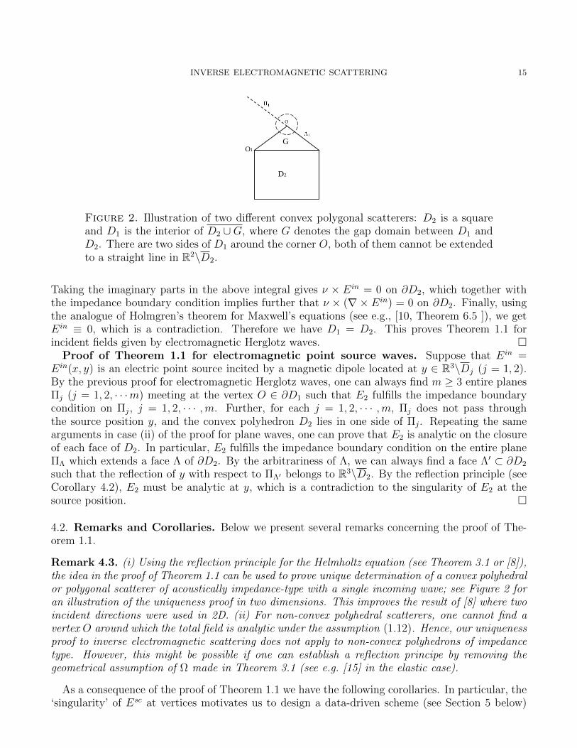
Figure 2. Illustration of two different convex polygonal scatterers: D2 is a squareand D1 is the interior of D2 ∪G, where G denotes the gap domain between D1 andD2. There are two sides of D1 around the corner O, both of them cannot be extendedto a straight line in R2\D2.

Taking the imaginary parts in the above integral gives ν × Ein = 0 on ∂D2, which together withthe impedance boundary condition implies further that ν × (∇× Ein) = 0 on ∂D2. Finally, usingthe analogue of Holmgren’s theorem for Maxwell’s equations (see e.g., [10, Theorem 6.5 ]), we getEin ≡ 0, which is a contradiction. Therefore we have D1 = D2. This proves Theorem 1.1 forincident fields given by electromagnetic Herglotz waves.

Proof of Theorem 1.1 for electromagnetic point source waves. Suppose that Ein =Ein(x, y) is an electric point source incited by a magnetic dipole located at y ∈ R3\Dj (j = 1, 2).By the previous proof for electromagnetic Herglotz waves, one can always find m ≥ 3 entire planesΠj (j = 1, 2, · · ·m) meeting at the vertex O ∈ ∂D1 such that E2 fulfills the impedance boundarycondition on Πj, j = 1, 2, · · · ,m. Further, for each j = 1, 2, · · · ,m, Πj does not pass throughthe source position y, and the convex polyhedron D2 lies in one side of Πj. Repeating the samearguments in case (ii) of the proof for plane waves, one can prove that E2 is analytic on the closureof each face of D2. In particular, E2 fulfills the impedance boundary condition on the entire planeΠΛ which extends a face Λ of ∂D2. By the arbitrariness of Λ, we can always find a face Λ′ ⊂ ∂D2

such that the reflection of y with respect to ΠΛ′ belongs to R3\D2. By the reflection principle (seeCorollary 4.2), E2 must be analytic at y, which is a contradiction to the singularity of E2 at thesource position.

4.2. Remarks and Corollaries. Below we present several remarks concerning the proof of The-orem 1.1.

Remark 4.3. (i) Using the reflection principle for the Helmholtz equation (see Theorem 3.1 or [8]),the idea in the proof of Theorem 1.1 can be used to prove unique determination of a convex polyhedralor polygonal scatterer of acoustically impedance-type with a single incoming wave; see Figure 2 foran illustration of the uniqueness proof in two dimensions. This improves the result of [8] where twoincident directions were used in 2D. (ii) For non-convex polyhedral scatterers, one cannot find avertex O around which the total field is analytic under the assumption (1.12). Hence, our uniquenessproof to inverse electromagnetic scattering does not apply to non-convex polyhedrons of impedancetype. However, this might be possible if one can establish a reflection principe by removing thegeometrical assumption of Ω made in Theorem 3.1 (see e.g. [15] in the elastic case).

As a consequence of the proof of Theorem 1.1 we have the following corollaries. In particular, the‘singularity’ of Esc at vertices motivates us to design a data-driven scheme (see Section 5 below)


to locate all vertices of D so that the position and shape of D can be recovered from a singlemeasurement data.

Corollary 4.4. Let D ⊂ R3 be a convex polyhedron and let E = Ein + Esc be the solution toEquations (1.2)-(1.5). Then E cannot be analytically extended from R3\D to the interior of Dacross a vertex of ∂D, or equivalently, E cannot be analytic on the vertices of D.

Corollary 4.5. Let D be a perfectly conduction polyhedron such that R3\D is connected. Supposethat E = Ein +Esc is a solution to Equations (1.2)-(1.4) with the boundary condition ν×E = 0 on∂D. If Ein is an incident Herglotz wave, we suppose additionally that k2 is not the eigenvalue of theoperator ∇×∇× over D with the boundary condition of vanishing tangential components on ∂D.Then ∂D can be uniquely determined by a single electric far-field pattern E∞ over all observationdirections. Moreover, E cannot be analytically extended from R3\D to the interior of D across avertex of ∂D.

Proof. Let Ein be an incident plane wave with the incident direction d ∈ S2 and polarizationdirection p ∈ S2. Suppose that two perfect polyhedral conductors D1 and D2 generate identicalelectric far-field patterns but D1 6= D2. Combining the path arguments of [29] and the uniquenessproof in Theorem 1.1 for incoming waves given by electromagnetic Herglotz waves, one can alwaysfind a perfectly conducting hyperplane Π ⊂ R3 such that Dj (j = 1 or j = 2) lies completely on oneside of Π. In fact, such a plane Π can be found by applying the ’point-to-point’ reflection principlewith the perfectly conducting boundary condition. This implies that the total electric field E canbe analytically extended into the whole space, leading to Esc ≡ 0 in R3 and thus ν × Ein = 0 on∂Dj. Hence, we get ν × p = 0 for any normal direction on ∂D, which is impossible.

If Ein is an electric Herglotz function, by the assumption of k2 one can also get the vanishingof Ein. In the case that Ein = Ein(x, y) is an electric point source wave emitting from the sourceposition y ∈ R3\Dj, one can prove that E2 satisfies the Dirichlet boundary condition on the entireplane which extends a face of D2; see the previous section in the impedance case. Using the “point-to-point” reflection principle together with the path argument, this could lead to the analyticity ofE2 at x = y, which is a contradiction to the singularity of E2 at the source position; see [19] in theacoustic case.

The impossibility of analytical extension across a vertex can by proved analogously.

Note that the perfectly conducting polyhedron in Corollary 4.5 is allowed to be non-convex, butcannot contain two-dimensional screens on its closure. The incident wave appearing in Corollaries4.4 and 4.5 can be a plane wave, Herglotz wave function or a point source wave.

4.3. Green’s tensor to the Maxwell’s equations in a half space with the impedanceboundary condition. As another application of the reflection principle, we derive the Green’stensor GI(x, y) ∈ C3×3 for the Maxwell’s equations in the half space R3

+ := x : x3 > 0 with theimpedance boundary condition enforcing on Π := x : x3 = 0, that is, for any constant vector~a ∈ R3,

∇× (∇×GI(x, y)~a)− k2GI(x, y)~a = δ(x− y)~a, in x3 > 0,

ν × (∇×GI(x, y)~a) + iλν × (ν ×GI(x, y)~a) = 0, on x3 = 0.(4.1)

For this purpose, we need the free-space Green’s tensor given by

G(x, y) := Φ(x, y)I +1

k2∇y∇yΦ(x, y), x 6= y,


where I is the 3× 3 identity matrix and ∇y∇yΦ(x, y) is the Hessian matrix for Φ defined by

(∇y∇yΦ(x, y))l,m =∂2Φ(x, y)

∂yl∂ym, 1 ≤ l,m ≤ 3, y = (y1, y2, y3) ∈ R3.

Note that here Φ(x, y) := 14π

eik|x−y|

|x−y| is the fundamental solution to Helmholtz equation in three

dimension.Following the arguments from [15, Corollary 2.2]), we can prove

Lemma 4.6. Denote by RΠ the reflection with respect to the plane Π and by Dx the action withrespect to x, of the operator D := (D1,D2,D3) defined in (3.5) and (3.6). Then the impedanceGreen’s tensor GI(x, y) can be represented as

GI(x, y) = G(x, y) +DxG(RΠx, y), x 6= y, x, y ∈ R3+.

Here the action of Dx on the tensor G is understood column-wisely.

5. A data-driven imaging scheme

The aim of this section is to establish a data-driven inversion scheme for imaging arbitrarilyconvex-polyhedral scatterers. Motivated by the one-wave factorization method in inverse elasticscattering [15], we shall propose a domain-defined indicator functional to characterize an inclusionrelationship between a test domain and our target; see also [18] in the acoustic case. Being differentfrom other domain-defined sampling approaches ( [24, 25, 31–33]) arising from inverse scattering,our scheme will be interpreted as a data-driven method, because it relies on measurement datacorresponding to a priori given test domains. In this paper, we shall take for simplicity perfectlyconducting balls with different centers and radii as test domains. Similar techniques were used inthe Extended Linear Sampling Method [30] for extracting information of a sound-soft obstacle froma single far-field pattern.

Consider the scattering of an incident plane wave Ein = ik (d× p) × deikx·d by a ball Bh(z) :=x ∈ R3 : |x − z| < h with h > 0, z ∈ R3, where d ∈ S2 is the incident direction and p ∈ R3 is apolarization vector. Then the total field E = Ein + Esc satisfies

∇× (∇× E)− k2E = 0 in |x− z| > h,

(ν × E)× ν = 0 on |x− z| = h,

lim|x|→∞(Esc × x+ 1

ik∇× Esc

)|x| = 0, x = x

r.

(5.1)

It is well known that (5.1) has a series solution E(x; d, p, h, z) for a given Ein(x; d, p) ( [35]). Fornotational convenience we will omit the dependance of solutions on d, p and k (all of them arefixed in our arguments) and only indicate the dependance on the center z ∈ R3 and radius h > 0of the ball Bh(z). Denote by E∞(x;h, z) the electric far-field pattern of the scattered electric fieldEsc. We expand E∞(x;h, z) into a series by using vector spherical harmonics. For any orthonormalsystem Y m

n , m = −n, . . . , n of spherical harmonics of order n > 0, the tangential fields defined onthe unit sphere

Umn (x) :=

1√n (n+ 1)

GradY mn (x); V m

n (x) := x× Umn (x)


are called vector spherical harmonics of order n. By coordinate translation, it is easy to check thatE∞ can be expanded into the convergent series ( [11,35])

E∞(x;h, z)eikz·x = 4π∞∑n=1

n∑m=−n

(u(h)n [Um

n (x) · p]Umn + v(h)

n [V mn · p]V m

n

)(5.2)

where

u(h)n :=

ψ′n(kh)

(ζ(1)n )′(kh)

∈ C, v(h)n := − ψ(kh)

ζ(1)n (kh)

∈ C,

with ψn(t) := tjn(t) and ζ(1)n (t) := th

(1)n (t). Here jn is the spherical Bessel function of order n

and h(1)n is the spherical Hankel function of first kind of order n. Denote the far-field operator

F (z,h) : T (S2) 7→ T (S2) by (F (z,h)g

)(x) :=

∫S2

E∞(x, d, g(d), h, z)ds(d)(5.3)

where T (S2) := g ∈ L2(S2)3 : g(x) · x = 0 for all x ∈ S2 denotes the tangential space defined onS2. The expression (5.2) shows that F (z,h) is diagonal in the basis

U (z)m,n(x) := e−ikz·xUm

n (x), V (z)m,n(x) := e−ikz·xV m

n (x).

It can be verified that(

4πu(h)n , 4πv

(h)n

)and

(U

(z)m,n, V

(z)m,n

)are eigenvalues and the associated eigen-

vectors of F (z,h). Note that the eigenvalues depend on the radius h only and the eigenfunctionsdepend on the location z only. We refer to [11] for detailed analysis when the ball is located at theorigin. The general case can be easily justified via coordinate translation.

To proceed, we suppose that w∞ ∈ T (S2) is the electric field pattern of some radiating electricfield wsc in |x| > b for some b > 0 sufficiently large. Introduce the function

Iw∞(z, h) :=1

4π

∞∑n=0

n∑m=−n

(|〈w∞, U (z)

m,n〉|2

|u(h)n |

+|〈w∞, V (z)

m,n〉|2

|v(h)n |

),(5.4)

where z ∈ R3 and h > 0 will be referred to as sampling variables in this paper. Equation (5.4) canbe regarded as a functional defined on the test domain Bh(z). If the above series is convergent, weshall prove below that the radiated electric field wsc can be analytically extended at least to theexterior of the test domain Bh(z). For simplicity we still denote by wsc the extended solution.

Lemma 5.1. Suppose that k2 is not the Dirichlet eigenvalue (that is, the tangential component ofthe electric field vanishes) of the operator curlcurl over the ball Bh(z). We have Iw∞(z, h) < ∞ ifand only if w∞ is the far-field pattern of the radiating field wsc which satisfies

(5.5) ∇× (∇× wsc)− k2wsc = 0 in |x− z| > h, ν × wsc × ν ∈ H−1/2curl (∂Bh(z)).

Here H−1/2curl (∂D) denotes the trace space of

H (curl,D) = φ ∈ (L2(D))3 : ∇× φ ∈ (L2(D))3of a bounded Lipschitz domain D ⊂ R3, given by

H−1/2curl (∂D) :=

u ∈

(H−1/2(∂D)

)3: ν · u = 0,∇× u ∈

(H−1/2(∂D)

)3on ∂D

.


Proof. Without loss of generality we may assume that Bh(z) is located at the origin, so that U(z)m,n =

Umn and V

(z)m,n = V m

n . Since the assumption on the wavenumber k ensures that (see [37, Chapter 5]for related discussions)

jn(t) 6= 0 and jn(t) + tj′n(t) 6= 0 for t = kh, n = 1, 2 · · · ,

we have |u(h)n | 6= 0 and |v(h)

n | 6= 0 for all n. By [10, Equation 6.73]) it follows that wsc can beexpressed as

wsc(x) =∞∑n=1

1

n(n+ 1)

n∑m=−n

[amn q

mn (x) + bmn∇× qmn (x)

]in |x| > b,

with the coefficients amn , bmn ∈ C and qmn (x) := ∇ × xh(1)

n (k|x|)Y mn (x). Correspondingly, the

far-field pattern w∞ is given by (see Equation (6.74) on page 219 in [10]):

w∞(x) =i

k

∞∑n=1

1

in+1

n∑m=−n

(ikbmn Umn (x)− amn V m

n (x)) .

Inserting the above expression into (5.4), we get

Iw∞(o, h) =1

4π

∞∑n=1

n∑m=−n

(|bmn |2

|u(h)n |

+|amn |2

|v(h)n |

), o = (0, 0, 0).(5.6)

To analyze the convergence of the above series, we need the asymptotic behavior of u(h)n and v

(h)n as

n→ +∞. Using the asymptotics of special functions for large orders, it is easy to observe that

1

|u(h)n |

=

∣∣∣∣∣∣∣(ζ

(1)n

)′ψ′n

∣∣∣∣∣∣∣ =

∣∣∣∣∣∣∣(th

(1)n (t)

)′(tjn(t))′

∣∣∣∣∣t=kh

∣∣∣∣∣∣∣ ∼∣∣∣∣∣∣∣(h

(1)n

)′(kh)

j′n(kh)

∣∣∣∣∣∣∣ ∼C1

|n|

∣∣∣(h(1)n

)′(kh)

∣∣∣2 ,1

|v(h)n |

=

∣∣∣∣∣ζ(1)n (kh)

ψn(kh)

∣∣∣∣∣ =

∣∣∣∣∣h(1)n (kh)

jn(kh)

∣∣∣∣∣ ∼ C2 |n| |h(1)n (kh)|2,

as n→∞, where C1, C2 ∈ C are fixed constants. Thus it follows from (5.6) that

Iw∞(o, h) ∼∞∑n=1

n∑m=−n

(C1|bmn |2|h

(1)n′(kh)|2

|n|+ C2|amn |2|n||h(1)

n (kh)|2)

(5.7)

On the other hand, it is seen from the expression of wsc that on |x| = h,

(x× wsc × x) =∞∑n=1

n∑m=−n

bmnh

(th(1)n (t)

)′ ∣∣∣t=kh

Umn (x)− amn h(1)

n (kh)V mn (x)

.


By definition of the H−1/2curl (∂Bh(z)) norm (see e.g. [37, Chapter 5] and [35, Chapter 9.3.3]) we obtain

‖x× wsc × x‖H−1/2curl (∂Bh(z))

=∞∑n=1

n∑m=−n

(1√

n (n+ 1)

|bmn |2

|h|2[(th(1)n (t)

)′ ∣∣∣t=kh

]2

+√n (n+ 1)|amn |2|h(1)

n (kh)|2)

∼∞∑n=1

n∑m=−n

(1

n|bmn |2|h(1)

n′(kh)|2 + n|amn |2|h(1)

n (kh)|2).(5.8)

Obviously, (5.7) and (5.8) have the same convergence. In the same manner, one can prove that(5.7) has the same convergence with ||ν × wsc||

H−1/2div (∂Bh(z))

where

H−1/2div (∂D) := u ∈

(H−1/2(∂D)

)3: ν · u = 0 on ∂D and (Div u) ∈ H−1/2(∂D).

Using the relation

||ν × wsc||L2(∂Bh(z)) + ||ν × wsc × ν||L2(∂Bh(z))

≤ C(||ν × wsc||

H−1/2div (∂Bh(z))

+ ||ν × wsc × ν||H−1/2curl (∂Bh(z))

),

we conclude that the tangential components of wsc on ∂Bh(z) are convergent in the L2-sense, ifIw∞(o, h) <∞. This together with [10, Theorem 6.27] implies that wsc is a solution to the Maxwell’sequations in |x| > h. The proof of Lemma 5.1 is thus complete.

Combining Lemma 5.1 and Corollary 4.4, we may characterize an inclusion relation between Dand Bh(z) through the measurement data E∞ of our target and the spectra of the far-field operatorF (z,h) corresponding to the test ball.

Theorem 5.2. Let E∞ be the electric far-field pattern of a convex-polyhedral scatterer D witha constant impedance coefficient. Suppose that k2 is not the Dirichlet eigenvalue of the operatorcurlcurl over the ball Bh(z). It holds that

IE∞(z, h) <∞ if and only if D ⊂ Bz(h).

Hence we have

D =

(z,h)⋂IE∞ (z,h)<∞

Bh(z).

Proof. If D ⊂ Bz(h), the scattered electric field Esc is well defined in x : |x − z| > h which liesin the exterior of D. Hence, Esc satisfies (5.5) and by Lemma 5.1 it holds that IE∞(z, h) <∞. On

the other hand, suppose that IE∞(z, h) <∞ but the relation D ⊂ Bz(h) does not hold. Since D isa convex polyhedron, there must exist at least one vertex O of ∂D such that |O − z| > h. Againusing Lemma 5.1, we conclude that Esc can be extended from R3\D to the exterior of Bh(z). Thisimplies that Esc is analytic at O, which contradicts Corollary 4.4.

By Theorem 5.2, the function h→ IE∞(z, h) for fixed |z| = R will blow up when h ≥ maxy∈∂D |y−z|, indicating a rough location of D with respect to z ∈ R3. In Table 5 we describe an inversionprocedure for imaging an arbitrary convex-polyhedron D by taking both z ∈ ∂BR and h as samplingvariables. The mesh for discretizing h ∈ (0, 2R) should be finer than the mesh for z ∈ ∂BR. Toavoid the assumption that k2 is not a Dirichlet eigenvalue of curl curl over Bh(z), one may use coatedballs by a thin dielectric layer (which can be modeled by the impedance boundary condition) as


Table 1. Data-driven scheme for imaging convex polyhedral scatterers

Step 1 Collect the measurement data E∞(x) for all x ∈ S2 and suppose that D ⊂ BR := x :|x| < R for some large R > 0.

Step 2 Choose sampling variables zj ∈ x : |x| = R and hi ∈ (0, 2R) to get the spectra of thefar-field operator F (z,h) corresponding to testing balls Bhj(zj) ⊂ BR.

Step 3 Calculate the domain-defined indicator function IE∞(zj, hi) by (5.4) with w∞ = E∞. Inparticular, it follows from Theorem 5.2 that

hi < maxy∈∂D

|zj − y| −→ IE∞(zj, hi) =∞,

hi ≥ maxy∈∂D

|zj − y| −→ IE∞(zj, hi) <∞.

Step 4 Image D as the intersection of all test balls Bhi(zj) such that IE∞(zj, hi) <∞.

test domains in place of our choice of perfectly conducting balls. We refer to [11, Section 3.1] fora description of the spectra of the far-field operator corresponding to such coated balls centeredat the origin. If the impedance coefficient is a positive constant, one can prove that k2 cannot bean impedance eigenvalue of curl curl over any boundary Lipschitz domain. It should be remarkedthat the test domains can also be taken as penetrable balls under the assumption that k2 is not aninterior transmission eigenvalue. Both Theorem 5.2 and Lemma 5.1 can be carried over to thesetest domains. Finally, it is worth mentioning that a regularization scheme should be employed to

truncate the series (5.6), because the eigenvalues u(h)n and v

(h)n decay very fast and the calculation

of the inner product between E∞ and the eigenfunctions(U

(z)n,m, V

(z)n,m

)is usually polluted by data

noise and numerical errors. We refer to [34] for numerical examples in inverse acoustic scattering.Numerical tests for Maxwell’s equations will be reported in our forthcoming publications.

Remark 5.3. In [33], the No Response Test was discussed for reconstructing convex perfectly con-ducting polyhedrons with two or a few incident electromagnetic plane waves. In comparison with [33],our inversion scheme uses only a single incoming wave within a more general class of plane waves,Herglotz wave functions and point source waves. Although both of them belong to the class of domain-defined sampling methods, the computational criterion explored here (see (5.4) and Theorem 5.2)involves simple inner product calculations and new sampling schemes due to the special choice oftesting balls.

Acknowledgments

The authors would like to thank the three anonymous referees for their comments and suggestionswhich help improve the original manuscript.

References

[1] G. Alessandrini and L. Rondi, Determining a sound-soft polyhedral scatterer by a single far-field measurement,Proc. Amer. Math. Soc., 6 (2005) 1685-91 (Corrigendum: http://arxiv.org/abs/math.AP/0601406).

[2] E. Blasten, L. Paivarinta and S. Sadique, Unique determination of the shape of a scattering screen from a passivemeasurement, Mathematics, 8 (2020): 1156.

[3] F. Cakoni and D. Colton, A Qualitative Approach to Inverse Scattering Theory, Springer, Newyork, 2014.


[4] F. Cakoni, D. Colton and P. Monk, The electromagnetic inverse scattering problem for partially coated Lip-schitz domains, Proceedings of the Royal Society of Edinburgh: Section A Mathematics 134 (2004): 661-682,doi:10.1017/S0308210500003413.

[5] D. Colton, H. Haddar and P. Monk, The linear sampling method for solving the electromagnetic inverse scatteringproblem, SIAM J. Sci. Comput. 24 (2002): 719-731.

[6] D. Colton, H. Haddar and M. Piana, The linear sampling method in inverse electromagnetic scattering theory,Inverse Problems 19 (2003): S105-S137.

[7] J. Cheng and M. Yamamoto, Uniqueness in an inverse scattering problem within non-trapping polygonal obsta-cles with at most two incoming waves, Inverse Problems, 19 (2003) 1361-84. (Corrigendum: Inverse Problems21 (2005): 1193)

[8] J. Cheng and M. Yamamoto, Global uniqueness in the inverse acoustic scattering problem within polygonalobstacles, Chinese Ann. Math. Ser. B 25 (2004), 1-6.

[9] D. Colton, A reflection principle for solutions to the Helmholtz equation and an application to the inversescattering problem Glasgow Math. J. 18 (1977): 125-130 .

[10] D. Colton and R. Kress, Inverse Acoustic and Electromagnetic Scattering Theory, 3nd edn, Berlin, Springer,2013.

[11] F. Collino, M. Fares and H. Haddar, Numerical and analytical studies of the linear sampling method in electro-magnetic inverse scattering problems, Inverse Problems, 19 (2003): 1279-1298.

[12] J. B. Diaz and G. S. Ludford, Reflection principles for linear elliptic second order partial differential equationswith constant coefficients, Ann. Mat. Pura Appl., 39 (1955): 87-95.

[13] J. Elschner and M. Yamamoto, Uniqueness in determining polygonal sound-hard obstacles with a single incomingwave, Inverse Problems, 22 (2006): 355-64.

[14] J. Elschner and M. Yamamoto, Uniqueness in inverse elastic scattering with finitely many incident waves, InverseProblems, 26 (2010): 045005.

[15] J. Elschner and G. Hu, Uniqueness and factorization method for inverse elastic scattering with a single incomingwave, Inverse Problems, 35 (2019): 094002.

[16] A. Friedman and V. Isakov, On the uniqueness in the inverse conductivity problem with one measurement,Indiana Univ. Math. J. 38 (1989): 563-579.

[17] N. Honda, G. Nakamura and M. Sini, Analytic extension and reconstruction of obstacles from few measurementsfor elliptic second order operators, Math. Ann., 355 (2013): 401-427.

[18] G. Hu and J. Li, Inverse source problems in an inhomogeneous medium with a single far-field pattern, to appearin: SIAM J. Math. Anal., 2020.

[19] G. Hu and X. Liu, Unique determination of balls and polyhedral scatterers with a single point source wave,Inverse Problems, 30 (2014): 065010.

[20] M. Ikehata, On reconstruction in the inverse conductivity problem with one measurement, Inverse Problems, 16(2000): 785–793.

[21] M. Ikehata, Reconstruction of a source domain from the Cauchy data, Inverse Problems, 15 (1999): 637–645.[22] A. Kirsch and N. Grinberg, The Factorization Method for Inverse Problems, Oxford Univ. Press, 2008.[23] A. Kirsch, The factorization method for Maxwell’s equations, Inverse Problems, 20 (2004): S117.[24] S. Kusiak, R. Potthast and J. Sylvester, A ‘range test’ for determining scatterers with unknown physical prop-

erties, Inverse Problems, 19 (2003): 533–547.[25] S. Kusiak and J. Sylvester, The scattering support, Communications on Pure and Applied Mathematics, 56

(2003): 1525–1548.[26] R. Kress, Uniqueness in inverse obstacle scattering for electromagnetic waves, Proceed-

ings of the URSI General Assembly 2002, Maastricht. Full proceedings available on CD viahttp://emctrans.virtualave.net/ursi/publications.htm

[27] C. Liu, An inverse obstacle problem: a uniqueness theorem for balls, In: Chavent G., Sacks P., PapanicolaouG., Symes W.W. (eds) Inverse Problems in Wave Propagation, The IMA Volumes in Mathematics and itsApplications, vol 90. Springer, New York, NY, 1997.

[28] H.Y. Liu and J. Zou, Uniqueness in an inverse acoustic obstacle scattering problem for both sound-hard andsound-soft polyhedral scatterers, Inverse Problems, 22 (2006): 515-524.

[29] H.Y. Liu, M. Yamamoto and J. Zou, Reflection principle for the Maxwell equations and its application to inverseelectromagnetic scattering, Inverse Problems, 23 (2007): 2357-2366.

[30] J. Liu and J. Sun, Extended sampling method in inverse scattering, Inverse Problems, 34 (2018): 085007.


[31] D. R. Luke and R. Potthast, The no response test –a sampling method for inverse scattering problems, SIAMJ. Appl. Math. 63 (2003): 1292-1312.

[32] R. Potthast, On the convergence of the no response test SIAM J. Math. Anal., 38 (2007): 1808-1824.[33] R. Potthast and M. Sini. The No-response Test for the reconstruction of polyhedral objects in electromagnetics,

J. Comp. Appl. Math, 234 (2010): 1739-1746.[34] G. Ma and G. Hu, A data-driven approach to inverse time-harmonic acoustic scattering, in preparation.[35] P. Monk, Finite Element Method for Maxwell’s Equations, Oxford University Press, Oxford, 2003.[36] G. Nakamura and R. Potthast, Inverse Modeling - an introduction to the theory and methods of inverse problems

and data assimilation, IOP Ebook Series, 2015.[37] J. C. Nedelec, Acoustic and Electromagnetic Equation. Integral Representation for Harmonic Problems, New

York, Spring, 2001.

†School of Mathematical Sciences and LPMC, Nankai University, Tianjin 300071, ChinaE-mail: [email protected]

‡Department of Mathematics, Indian Institute of Technology, Jammu 181221, IndiaE-mail: [email protected]

∗School of Mathematics and Statistics, Xi’an Jiaotong University, Xi’an 710049, P. R. China.E-mail: [email protected]

Documents

INVERSE TIME-HARMONIC ELECTROMAGNETIC SCATTERING …