Inverse Problems and Regularization – An Introduction

Inverse Problems and Regularization –An Introduction

Stefan KindermannIndustrial Mathematics Institute

University of Linz, Austria

Introduction to Regularization

What are Inverse Problems ?

One possible definition [Engl, Hanke, Neubauer ’96]:Inverse problems are concerned with determining causes for adesired or an observed effect.

Cause(Parameter, Unknown,

Solution of Inv. Prob, . . .)

Direct Problem=⇒

Inverse Problem⇐=

Effect(Data, Observation, . . .)


Direct and Inverse Problems

The classification as direct or inverse is in the most cases based onthe well/ill-posedness of the associated problems:

Cause

Stable=⇒

Unstable⇐=

Effect

Inverse Problems ∼ Ill-posed/(Ill-conditioned) Problems


What are Inverse Problems?

A central feature of inverse problems is their ill-posedness

Well-Posedness in the sense of Hadamard [Hadamard ’23]

Existence of a solution (for all admissible data)

Uniqueness of a solution

Continuous dependence of solution on the data

Well-Posedness in the sense of Nashed [Nashed, ’87]

A problem is well posed if the set of Data/Observations is a closedset. (The range of the forward operator is closed).


Abstract Inverse Problem

Abstract inverse problem:Solve equation for x ∈ X (Banach/Hilbert- ... space), given datay ∈ Y (Banach/Hilbert- ... space)

F (x) = y ,

where F−1 does not exist or is not continuous.

F . . . forward operator

We want′′x† = F−1(y)′′

x†.. (generalized) solution



• If the forward operator is linear ⇒ linear inverse problem.• A linear inverse problem is well-posed in the sense of Nashed ifthe range of F is closed.

Theorem: An linear operator with finite dimensional range isalways well-posed (in Nashed’s sense).

“Ill-posedness lives in infinite dimensional spaces”



“Ill-posedness lives in infinite dimensional spaces”Problems with a few number of parameters usually do not needregularization.Discretization acts as Regularization/Stabilization

Ill-posedness in finite dimensional space ∼ Ill-conditioning

Measure of ill-posedness: decay of singular values of forwardoperator


Methodologies in studying Inverse Problems

Deterministic Inverse Problems(Regularization, worst case convergence, infinite di-

mensional, no assumptions on noise)

Statistics(Estimators, average case analysis, often finite di-

mensional, noise is random variable, specific struc-

ture )

Bayesian Inverse Problems(Posteriori distribution, finite dimensional, analysis

of post. dist. by estimators, specific assumptions

on noise and prior)

Control Theory(x= control, F (x)= state, convergence of state not

control, infinite dimensional, no assumptions)


Deterministic Inverse Problems and Regularization

Try to solveF (x) = y ,

when′′x† = F−1(y)′′

does not exist.

Notation: x† the “true” (unknown) solution (minimal normsolution)

Even if F−1(y) exists, it might not be computable [Pour-El, Richards ’88]



Data noise: Usually we do not have the exact data

y = F (x†)

but only noisy data

yδ = F (x†) + noise

Amount of noise: noiselevel

δ = ‖F (x†)− yδ‖



Method to solve Ill-posed problems:Regularization: Approximate the inverse F−1 by a family ofstable operators Rα

F (x) = y

“x† = F−1(y)“ ⇒ xα = Rα(y)

Rα ∼ F−1

Rα Regularization operators

α Regularization parameter


Regularization

α small ⇒ Rα good approximation for F−1, but unstable

α large ⇒ Rα stable but bad approximation for F−1,

α ... controls Trade-off between approximation and stability.Total error = approximation error + propagated data error

Approximation Error →

Propagated← Data Error

Total Error↓

α

||xα−

x||

How to select α: Parameter choice rulesIntroduction to Regularization

Example: Tikhonov Regularization

Tikhonov Regularization: [Phillips ’62; Tikhonov ’63]

Let F : X → Y be linear between Hilbertspaces:A least squares solution to F (x) = y is given by the normalequations

F ∗Fx = F ∗y

Tikhonov regularization: Solve regularized problem

F ∗Fx + αx = F ∗y

xα = (F ∗F + αI )−1F ∗y


Example: Tikhonov Regularization

Error estimates (under some conditions)

‖xα − x†‖2 ≤ δ2

α+ Cαν

total Error (Stability) Approx.

Theory of linear and nonlinear problems in Hilbert spaces:[Tikhonov, Arsensin ’77; Groetsch ’84; Hofmann ’86; Baumeister ’87, Louis ’89;

Kunisch, Engl, Neubauer ’89; Bakushinskii, Goncharskii ’95; Engl, Hanke, Neubauer

’96; Tikhonov, Leonov, Yagola ’98; . . . ]


Example: Landweber iteration

Landweber iteration [Landweber ’51]

Solve normal equation by Richardson iterationLandweber iteration

xk+1 = xk − F ∗(F (xk)− y) k = 0, . . .

Iteration index is the regularization parameter α = 1k


Example: Landweber iteration

Error estimates (under some conditions)

‖xk − x†‖2 ≤ kδ +C

kν

total Error (Stability) Approx.

Semiconvergence

Iterative Regularization Methods:Parameter choice = choice of stopping index k

Theory: [Landweber ’51; Fridman ’56; Bialy ’59; Strand ’74; Vasilev ’83; Groetsch

’85; Natterer ’86; Hanke, Neubauer, Scherzer ’95; Bakushinskii, Goncharskii ’95;

Engl, Hanke, Neubauer ’96;. . . ]


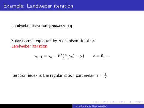
Notion of Convergence

Does the regularized solution converges to the true solution as thenoise level tends to 0

limδ→0

xα → x†

(Worst case) convergence

limδ→0

sup‖xα − x†‖ | ∀yδ : ‖yδ − F (x†)‖ ≤ δ = 0

(for a given parameter choice rule)

Convergence in expectation

E‖xα − x†‖2 → 0 as E‖yδ − F (x†)‖2 → 0


Theory of Regularization of Inverse Problems

Convergence depends on x†

Question of speed: convergence rates

‖xα − x†‖ ≤ f (α) or ‖xα − x†‖ ≤ f (δ)


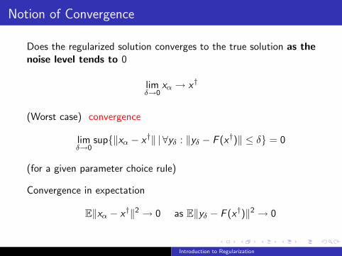
Theoretical Results

[Schock ’85]: Convergence can be arbitrarily slow !

Theorem: For ill-posed problems in the sense of Nashed, therecannot be a function f with limδ→ f (δ) = 0 such that for all x†

‖xα − x†‖ ≤ f (δ)

Uniform bounds on the convergence rates are impossible

Convergence rates are possible if x† in some smoothness class


Theoretical Results

Convergence rates: requires a source condition

x† ∈M

Convergence rates ∼ modulus of continuity of the inverse

Ω(δ,M) = sup‖x†1−x†2‖ | ‖F (x†1)−F (x†2)‖ ≤ δ, x†1, x†2 ∈M

Theorem[Tikhonov, Arsenin ’77, Morozov ’92, Traub, Wozniakowski ’80]

For an arbitrary regularization map, arbitrary parameter choice rule(with Rα(0) = 0)

‖xα − x†‖ ≥ Ω(δ,M)


Theoretical Results

Standard smoothness classes:For linear ill-posed problems in Hilbert spaces we can form

M = Xµ = x† = (F ∗F )νω |ω ∈ X

(Holder) source condition (=abstract smoothness condition)

Ω(δ,Xµ) = Cδ2µ

2µ+1

Best convergence rate for Holder source conditions

A regularization operator and a parameter choice rule such that

‖xα − x†‖ = Cδ2µ

2µ+1

is called order optimal.


Theoretical Results

Special casex† = F ∗ω

Such source conditions can be generalized to nonlinear problemse.g.

x† = F ′(x†)∗ω

x† = (F ′(x†)∗F (x†))νω


Theoretical Results

Many regularization method have shown to be order optimal.A significant amount of theoretical results in regularization theorydeals with this issue:

Convergence of method and parameter choice rule

Optimal order convergence under source condition.

Knowledge of the source condition does not have to be known.


Parameter Choice Rules

How to choose the regularization parameter:Classification

a-priori α = α(δ)

a-posteriori α = α(δ, y)

heuristic α = α(y)


Bakushinskii veto

Bakushinskii veto: [Bakushinskii ’84] A parameter choice withoutknowledge of δ cannot yield a convergent regularization in theworst case (for ill-posed problems).

Knowledge of δ is needed !

⇒ heuristic parameter choice rules are nonconvergent in the worstcase


a-priori-rules

Example of a-priori rule:

If x† ∈ Xµ, then

α = δ1

2µ+1

yields optimal order for Tikhonov regularization

+ Easy to implement

− Needs information on source condition


a-posteriori rules

Example a-posteriori rules:Morozov’s Discrepancy principle: [Morozov ’66]

Fix τ > 1,DP: Choose the largest α such that the residual is of the order ofthe noise level

‖F (xα)− y‖ ≤ τδYields in many situations a optimal order method

+ Easy to implement

+ No information on source conditions

− In some cases not optimal order

Other a-posteriori choice rules:

Gferer-Raus-Rule (improved discrepancy principle) [Raus ’85;

Gferer ’87]

Balancing principle [Lepski ’90; Mathe, Pereverzev ’03]

. . .


Heuristic Parameter Choice rules

Example heuristic rules:

Quasi-optimality Rule [Tikhonov, Glasko ’64]

Choose a sequence of geometrically decaying regularizationparameter

αn = Cqn q < 1

For each α compute xαn

Choose α = αn∗ where n∗ is the minimizer of

‖xαn+1 − xαn‖


Heuristic Parameter Choice rules

Example heuristic rules:

Hanke-Raus Rule [Hanke, Raus ’96]

Choose α as minimizer of

1√α‖F (xα)− y‖


Heuristic Parameter Choice rules: Theory

Heuristic Rules cannot converge in the worst case:

Convergence in the restricted noise case [K., Neubauer ’08, K. ’11]

limδ→0‖xα − x†‖ → 0 if yδ = F (x) + noise, noise ∈ N

The conditionnoise ∈ N

is an abstract noise condition.


Heuristic Parameter Choice rules: Theory

In the linear case reasonable noise conditions can be stated andconvergence and convergence rates can be shown:

Noise condition: ”Data noise has to be sufficiently irregular”


Nonlinear Case :Tikhonov Regularization

F (x) = y

with F nonlinear

Tikhonov Regularization for Nonlinear Problems[Tikhonov, Arsenin ’77; Engl, Kunisch Neubauer, ’89; Neubauer ’89, . . . ]

xα is a (global) minimizer of the Tikhonov functional

J(x) = ‖F (x)− y‖2 + αR(x)

R(x) is a regularization functional



Convergence (Rates) Theory:

Hilbert spaces [Engl, Kunisch Neubauer ’89; Neubauer ’89]

Banach spaces [Kaltenbacher, Hofmann, Poschl, Scherzer ’08]

Parameter Choice rules:a-priori: α = δξ

a-posteriori: Discrepancy principle



Examples: Sobolev norm

R(x) = ‖x‖2Hs

Total Variation

R(x) =

∫|∇x |

L1-norm

R(x) =

∫|x |

Maximum Entropy

R(x) =

∫|x | log(x)



Choice of the Regularization functional:Deterministic Theory: User can choose:

Should stabilize problem

Convergence theory should apply

R(x) should reflect what we expect from solution

Bayesian viewpoint: Regularization functional ∼ prior



Computational issue:

The regularized solution is a global minimum of a optimizationproblemxα is a (global) minimizer

J(x) = ‖F (x)− y‖2 + αR(x)


Iterative Methods

Example:Nonlinear Landweber iteration [Hanke, Neubauer, Scherzer ’95]

xk+1 = xk − F ′(xk)∗(F (xk)− y)

Parameter choice by choosing the stopping index.Convergence rates theory needs a nonlinearity condition

‖F (x)− F (x†)− F ′(x†)(x − x†)‖ ≤ C‖F (x)− F (x†)‖

Restricts the nonlinearity of the problemVariants of a nonlinearity condition

Range-invariance [Blaschke/Kaltenbacher ’96]

Curvature condition [Chavent, Kunisch ’98]

Variational inequalities [Kaltenbacher, Hofmann, Poschl, Scherzer ’08]

Faster alternative: Gauss-Newton type iterations [Bakushinskii ’92,

Blaschke, Neubauer, Scherzer ’97]


Summary

Theoretical issues:For a given inverse problem

Understand ill-posedness (Uniqueness/Stability)

Are data rich enough to characterize solution uniquely

How unstable is the inverse problem (degree of ill-posedness)

Method of Regularization + Parameter Choice

Design efficient regularization method for class of problem

Convergence, Convergence rates (optimal order),

Interplay: Regularization, Discretization

Practical issues:

How to compute global optimum in TR (efficiently)

Improving iterative methods (Newton-type, preconditioning)

What Regularization term to choose


Dynamic Inverse Problems

Forward operator/Solution x(t) depend on time

F (x(t ′ ≤ t), t) = y(t)


Dynamic Inverse Problems

Examples:Volterra integral equation of the first kind∫ t

0k(t, s)x(s)ds = y(t)

Parameter identification in ODEs

y ′(t) = f (t, y(t), x(t))

Control theory

z(t)′ = Az(t) + Bx(t)

y(t)′ = Cz(t) + Dx(t)


Methods

Example: Tikhonov Regularization∫ T

0‖F (t, x(., t))− y(t)‖2dt + αR(x(t)

+ Convergence

− Not causal/sequential: Computation of x(t) requires alldata (past/future)


Methods

Alternative:Dynamic Programing [K.,Leitao ’06]

x ′(t) = G (x(t),V (t))

+ Convergence

− Only for linear problems

− Partially causal/sequential: Computation of V (t) requiresall data (past/future)


Methods

Control Theoretic Methods:Feedback control

x(t) = Ky(t)

(x(t), x ′(t)) = Ky(t)

−Convergence in x (Asymptotic convergence)?

− Fully causal/sequential: Computation of x(t) requires onlydata (at t)

+ Nonlinear


Methods

Control Theoretic Methods:Kalman filter

− Restrictive Assumptions on noise

+ Fully causal/sequential


Methods

Local Regularization [Lamm, Scofield ’01; Lamm ’03]

xα(t) is given by an ODE related to Volterra equation


+ Convergence theory

+ Nonlinear

− Quite specific method for Volterra equations


Methods

Kugler’ online parameter identification [Kugler ’08]

x ′(t) = G (x(t))∗(F (x(t))− y(t))


+ Asymptotic convergence theory (also for nonlinear case)

− Assumptions realistic ?

− Assumes x does not depend on time


The wanted method

fully causal/sequential method

convergence theory in the illposed and nonlinear case

no/weak assumptions on operator

no/weak assumptions on solution

no assumption on noise

efficient to compute


Documents

Inverse Problems and Regularization – An Introduction